
Numerical Methods in Science and Engineering
Thomas R. Bewley
UC San Diego
i

ii

Contents
Preface
vii
1 A short review of linear algebra
1
1.1 Notation . . . . . . . . . . . . . . . . . . . . . . . . . . . . . . . . . . . . . . . . . . .
1
1.1.1 Vectors . . . . . . . . . . . . . . . . . . . . . . . . . . . . . . . . . . . . . . .
1
1.1.2 Vector addition . . . . . . . . . . . . . . . . . . . . . . . . . . . . . . . . . . .
1
1.1.3 Vector multiplication . . . . . . . . . . . . . . . . . . . . . . . . . . . . . . . .
2
1.1.4 Matrices . . . . . . . . . . . . . . . . . . . . . . . . . . . . . . . . . . . . . . .
2
1.1.5 Matrix addition . . . . . . . . . . . . . . . . . . . . . . . . . . . . . . . . . . .
2
1.1.6 Matrix/vector multiplication . . . . . . . . . . . . . . . . . . . . . . . . . . .
3
1.1.7 Matrix multiplication . . . . . . . . . . . . . . . . . . . . . . . . . . . . . . .
3
1.1.8 Identity matrix . . . . . . . . . . . . . . . . . . . . . . . . . . . . . . . . . . .
4
1.1.9 Inverse of a square matrix . . . . . . . . . . . . . . . . . . . . . . . . . . . . .
4
1.1.10 Other denitions . . . . . . . . . . . . . . . . . . . . . . . . . . . . . . . . . .
4
1.2 Determinants . . . . . . . . . . . . . . . . . . . . . . . . . . . . . . . . . . . . . . . .
6
1.2.1 Denition of the determinant . . . . . . . . . . . . . . . . . . . . . . . . . . .
6
1.2.2 Properties of the determinant . . . . . . . . . . . . . . . . . . . . . . . . . . .
6
1.2.3 Computing the determinant . . . . . . . . . . . . . . . . . . . . . . . . . . . .
6
1.3 Eigenvalues and Eigenvectors . . . . . . . . . . . . . . . . . . . . . . . . . . . . . . .
7
1.3.1 Physical motivation for eigenvalues and eigenvectors . . . . . . . . . . . . . .
7
1.3.2 Eigenvector decomposition . . . . . . . . . . . . . . . . . . . . . . . . . . . .
9
1.4 Matrix norms . . . . . . . . . . . . . . . . . . . . . . . . . . . . . . . . . . . . . . . . 10
1.5 Condition number . . . . . . . . . . . . . . . . . . . . . . . . . . . . . . . . . . . . . 10
2 Solving linear equations
11
2.1 Introduction to the solution of
A
x
=
b
. . . . . . . . . . . . . . . . . . . . . . . . . . 11
2.1.1 Example of solution approach . . . . . . . . . . . . . . . . . . . . . . . . . . . 12
2.2 Gaussian elimination algorithm . . . . . . . . . . . . . . . . . . . . . . . . . . . . . . 14
2.2.1 Forward sweep . . . . . . . . . . . . . . . . . . . . . . . . . . . . . . . . . . . 14
2.2.2 Back substitution . . . . . . . . . . . . . . . . . . . . . . . . . . . . . . . . . . 14
2.2.3 Operation count . . . . . . . . . . . . . . . . . . . . . . . . . . . . . . . . . . 15
2.2.4 Matlab implementation . . . . . . . . . . . . . . . . . . . . . . . . . . . . . . 16
2.2.5
LU
decomposition . . . . . . . . . . . . . . . . . . . . . . . . . . . . . . . . . 17
2.2.6 Testing the Gaussian elimination code . . . . . . . . . . . . . . . . . . . . . . 19
2.2.7 Pivoting . . . . . . . . . . . . . . . . . . . . . . . . . . . . . . . . . . . . . . . 19
2.3 Thomas algorithm . . . . . . . . . . . . . . . . . . . . . . . . . . . . . . . . . . . . . 20
2.3.1 Forward sweep . . . . . . . . . . . . . . . . . . . . . . . . . . . . . . . . . . . 20
iii

2.3.2 Back substitution . . . . . . . . . . . . . . . . . . . . . . . . . . . . . . . . . . 21
2.3.3 Operation count . . . . . . . . . . . . . . . . . . . . . . . . . . . . . . . . . . 21
2.3.4 Matlab implementation . . . . . . . . . . . . . . . . . . . . . . . . . . . . . . 22
2.3.5
LU
decomposition . . . . . . . . . . . . . . . . . . . . . . . . . . . . . . . . . 22
2.3.6 Testing the Thomas code . . . . . . . . . . . . . . . . . . . . . . . . . . . . . 23
2.3.7 Parallelization . . . . . . . . . . . . . . . . . . . . . . . . . . . . . . . . . . . 24
2.4 Review . . . . . . . . . . . . . . . . . . . . . . . . . . . . . . . . . . . . . . . . . . . . 24
3 Solving nonlinear equations
25
3.1 The Newton-Raphson method for nonlinear root nding . . . . . . . . . . . . . . . . 25
3.1.1 Scalar case . . . . . . . . . . . . . . . . . . . . . . . . . . . . . . . . . . . . . 25
3.1.2 Quadratic convergence . . . . . . . . . . . . . . . . . . . . . . . . . . . . . . . 26
3.1.3 Multivariable case|systems of nonlinear equations . . . . . . . . . . . . . . . 27
3.1.4 Matlab implementation . . . . . . . . . . . . . . . . . . . . . . . . . . . . . . 28
3.1.5 Dependence of Newton-Raphson on a good initial guess . . . . . . . . . . . . 29
3.2 Bracketing approaches for scalar root nding . . . . . . . . . . . . . . . . . . . . . . 30
3.2.1 Bracketing a root . . . . . . . . . . . . . . . . . . . . . . . . . . . . . . . . . . 30
3.2.2 Rening the bracket - bisection . . . . . . . . . . . . . . . . . . . . . . . . . . 31
3.2.3 Rening the bracket - false position . . . . . . . . . . . . . . . . . . . . . . . 32
3.2.4 Testing the bracketing algorithms . . . . . . . . . . . . . . . . . . . . . . . . . 33
4 Interpolation
35
4.1 Lagrange interpolation . . . . . . . . . . . . . . . . . . . . . . . . . . . . . . . . . . . 35
4.1.1 Solving
n
+ 1 equations for the
n
+ 1 coecients . . . . . . . . . . . . . . . . 35
4.1.2 Constructing the polynomial directly . . . . . . . . . . . . . . . . . . . . . . . 36
4.1.3 Matlab implementation . . . . . . . . . . . . . . . . . . . . . . . . . . . . . . 37
4.2 Cubic spline interpolation . . . . . . . . . . . . . . . . . . . . . . . . . . . . . . . . . 37
4.2.1 Constructing the cubic spline interpolant . . . . . . . . . . . . . . . . . . . . 38
4.2.2 Matlab implementation . . . . . . . . . . . . . . . . . . . . . . . . . . . . . . 41
4.2.3 Tension splines . . . . . . . . . . . . . . . . . . . . . . . . . . . . . . . . . . . 43
4.2.4 B-splines . . . . . . . . . . . . . . . . . . . . . . . . . . . . . . . . . . . . . . 43
5 Minimization
45
5.0 Motivation . . . . . . . . . . . . . . . . . . . . . . . . . . . . . . . . . . . . . . . . . 45
5.0.1 Solution of large linear systems of equations . . . . . . . . . . . . . . . . . . . 45
5.0.2 Solution of nonlinear systems of equations . . . . . . . . . . . . . . . . . . . . 45
5.0.3 Optimization and control of dynamic systems . . . . . . . . . . . . . . . . . . 46
5.1 The Newton-Raphson method for nonquadratic minimization . . . . . . . . . . . . . 46
5.2 Bracketing approaches for minimization of scalar functions . . . . . . . . . . . . . . . 47
5.2.1 Bracketing a minimum . . . . . . . . . . . . . . . . . . . . . . . . . . . . . . . 47
5.2.2 Rening the bracket - the golden section search . . . . . . . . . . . . . . . . . 48
5.2.3 Rening the bracket - inverse parabolic interpolation . . . . . . . . . . . . . . 50
5.2.4 Rening the bracket - Brent's method . . . . . . . . . . . . . . . . . . . . . . 52
5.3 Gradient-based approaches for minimization of multivariable functions . . . . . . . . 52
5.3.1 Steepest descent for quadratic functions . . . . . . . . . . . . . . . . . . . . . 54
5.3.2 Conjugate gradient for quadratic functions . . . . . . . . . . . . . . . . . . . 55
5.3.3 Preconditioned conjugate gradient . . . . . . . . . . . . . . . . . . . . . . . . 59
5.3.4 Extension non-quadratic functions . . . . . . . . . . . . . . . . . . . . . . . . 61
iv

6 Dierentiation
63
6.1 Derivation of nite dierence formulae . . . . . . . . . . . . . . . . . . . . . . . . . . 63
6.2 Taylor Tables . . . . . . . . . . . . . . . . . . . . . . . . . . . . . . . . . . . . . . . . 64
6.3 Pade Approximations . . . . . . . . . . . . . . . . . . . . . . . . . . . . . . . . . . . 65
6.4 Modied wavenumber analysis . . . . . . . . . . . . . . . . . . . . . . . . . . . . . . 67
6.5 Alternative derivation of dierentiation formulae . . . . . . . . . . . . . . . . . . . . 68
7 Integration
69
7.1 Basic quadrature formulae . . . . . . . . . . . . . . . . . . . . . . . . . . . . . . . . . 69
7.1.1 Techniques based on Lagrange interpolation . . . . . . . . . . . . . . . . . . . 69
7.1.2 Extension to several gridpoints . . . . . . . . . . . . . . . . . . . . . . . . . . 70
7.2 Error Analysis of Integration Rules . . . . . . . . . . . . . . . . . . . . . . . . . . . . 70
7.3 Romberg integration . . . . . . . . . . . . . . . . . . . . . . . . . . . . . . . . . . . . 71
7.4 Adaptive Quadrature . . . . . . . . . . . . . . . . . . . . . . . . . . . . . . . . . . . . 74
8 Ordinary dierential equations
77
8.1 Taylor-series methods . . . . . . . . . . . . . . . . . . . . . . . . . . . . . . . . . . . 77
8.2 The trapezoidal method . . . . . . . . . . . . . . . . . . . . . . . . . . . . . . . . . . 78
8.3 A model problem . . . . . . . . . . . . . . . . . . . . . . . . . . . . . . . . . . . . . . 79
8.3.1 Simulation of an exponentially-decaying system . . . . . . . . . . . . . . . . . 79
8.3.2 Simulation of an undamped oscillating system . . . . . . . . . . . . . . . . . . 79
8.4 Stability . . . . . . . . . . . . . . . . . . . . . . . . . . . . . . . . . . . . . . . . . . . 82
8.4.1 Stability of the explicit Euler method . . . . . . . . . . . . . . . . . . . . . . 82
8.4.2 Stability of the implicit Euler method . . . . . . . . . . . . . . . . . . . . . . 83
8.4.3 Stability of the trapezoidal method . . . . . . . . . . . . . . . . . . . . . . . . 83
8.5 Accuracy . . . . . . . . . . . . . . . . . . . . . . . . . . . . . . . . . . . . . . . . . . 84
8.6 Runge-Kutta methods . . . . . . . . . . . . . . . . . . . . . . . . . . . . . . . . . . . 85
8.6.1 The class of second-order Runge-Kutta methods (RK2) . . . . . . . . . . . . 85
8.6.2 A popular fourth-order Runge-Kutta method (RK4) . . . . . . . . . . . . . . 87
8.6.3 An adaptive Runge-Kutta method (RKM4) . . . . . . . . . . . . . . . . . . . 88
8.6.4 A low-storage Runge-Kutta method (RKW3) . . . . . . . . . . . . . . . . . . 89
A Getting started with Matlab
1
A.1 What is Matlab? . . . . . . . . . . . . . . . . . . . . . . . . . . . . . . . . . . . . . .
1
A.2 Where to nd Matlab . . . . . . . . . . . . . . . . . . . . . . . . . . . . . . . . . . .
1
A.3 How to start Matlab . . . . . . . . . . . . . . . . . . . . . . . . . . . . . . . . . . . .
2
A.4 How to run Matlab|the basics . . . . . . . . . . . . . . . . . . . . . . . . . . . . . .
2
A.5 Commands for matrix factoring and decomposition . . . . . . . . . . . . . . . . . . .
6
A.6 Commands used in plotting . . . . . . . . . . . . . . . . . . . . . . . . . . . . . . . .
7
A.7 Other Matlab commands . . . . . . . . . . . . . . . . . . . . . . . . . . . . . . . . .
8
A.8 Hardcopies . . . . . . . . . . . . . . . . . . . . . . . . . . . . . . . . . . . . . . . . .
8
A.9 Matlab programming procedures: m-les . . . . . . . . . . . . . . . . . . . . . . . . .
8
A.10 Sample m-le . . . . . . . . . . . . . . . . . . . . . . . . . . . . . . . . . . . . . . . .
9
v

vi

Preface
The present text provides a brief (one quarter) introduction to ecient and eective numerical
methods for solving typical problems in scientic and engineering applications. It is intended to
provide a succinct and modern guide for a senior or rst-quarter masters level course on this subject,
assuming only a prior exposure to linear algebra, a knowledge of complex variables, and rudimentary
skills in computer programming.
I am indebted to several sources for the material compiled in this text, which draws from class
notes from ME200 by Prof. Parviz Moin at Stanford University, class notes from ME214 by Prof.
Harv Lomax at Stanford University, and material presented in Numerical Recipes by Press et al.
(1988-1992) and Matrix Computations by Golub & van Loan (1989). The latter two textbooks are
highly recommended as supplemental texts to the present notes. We do not attempt to duplicate
these excellent texts, but rather attempt to build up to and introduce the subjects discussed at
greater lengths in these more exhaustive texts at a metered pace.
The present text was prepared as supplemental material for MAE107 and MAE290a at UC San
Diego.
vii

viii

Chapter
1
A short review of linear algebra
Linear algebra forms the foundation upon which ecient numerical methods may be built to solve
both linear and nonlinear systems of equations. Consequently, it is useful to review briey some
relevant concepts from linear algebra.
1.1 Notation
Over the years, a fairly standard notation has evolved for problems in linear algebra. For clarity,
this notation is now reviewed.
1.1.1 Vectors
A vector is dened as an ordered collection of numbers or algebraic variables:
c
=
0
B
B
B
@
c
1
c
2
...
c
n
1
C
C
C
A
:
All vectors in the present notes will be assumed to be arranged in a column unless indicated otherwise.
Vectors are represented with lower-case letters and denoted in writing (i.e., on the blackboard) with
an arrow above the letter (
~c
) and in print (as in these notes) with boldface (
c
). The vector
c
shown
above is
n
-dimensional, and its
i
'th element is referred to as
c
i
. For simplicity, the elements of all
vectors and matrices in these notes will be assumed to be real unless indicated otherwise. However,
all of the numerical tools we will develop extend to complex systems in a straightforward manner.
1.1.2 Vector addition
Two vectors of the same size are added by adding their individual elements:
c
+
d
=
0
B
B
B
@
c
1
+
d
1
c
2
+
d
2
...
c
n
+
d
n
1
C
C
C
A
:
1

2
CHAPTER
1.
A
SHOR
T
REVIEW
OF
LINEAR
ALGEBRA
1.1.3 Vector multiplication
In order to multiply a vector with a scalar, operations are performed on each element:
c
=
0
B
B
B
@
c
1
c
2
...
c
n
1
C
C
C
A
:
The
inner product
of two real vectors of the same size, also known as
dot product
, is dened
as the sum of the products of the corresponding elements:
(
u
v
) =
u
v
=
n
X
i
=1
u
i
v
i
=
u
1
v
1
+
u
2
v
2
+
:::
+
u
n
v
n
:
The
2-norm of a vector
, also known as the
Euclidean norm
or the
vector length
, is dened
by the square root of the inner product of the vector with itself:
k
u
k
=
p
(
u
u
) =
q
u
21
+
u
22
+
:::
+
u
2
n
:
The
angle between two vectors
may be dened using the inner product such that
cos
]
(
u
v
) = (
u
v
)
k
u
k
k
v
k
:
In
summation notation
, any term in an equation with lower-case English letter indices repeated
twice implies summation over all values of that index. Using this notation, the inner product is
written simply as
u
i
v
i
. To avoid implying summation notation, Greek indices are usually used.
Thus,
u
v
does not imply summation over
.
1.1.4 Matrices
A matrix is dened as a two-dimensional ordered array of numbers or algebraic variables:
A
=
0
B
B
B
@
a
11
a
12
::: a
1
n
a
21
a
22
::: a
2
n
... ... ... ...
a
m
1
a
m
2
::: a
mn
1
C
C
C
A
:
The matrix above has
m
rows and
n
columns, and is referred to as an
m
n
matrix. Matrices
are represented with uppercase letters, with their elements represented with lowercase letters. The
element of the matrix
A
in the
i
'th row and the
j
'th column is referred to as
a
ij
.
1.1.5 Matrix addition
Two matrices of the same size are added by adding their individual elements. Thus, if
C
=
A
+
B
,
then
c
ij
=
a
ij
+
b
ij
.

1.1.
NOT
A
TION
3
1.1.6 Matrix/vector multiplication
The product of a matrix
A
with a vector
x
, which results in another vector
b
, is denoted
A
x
=
b
.
It may be dened in index notation as:
b
i
=
n
X
j
=1
a
ij
x
j
:
In summation notation, it is written:
b
i
=
a
ij
x
j
:
Recall that, as the
j
index is repeated in the above expression, summation over all values of
j
is
implied without being explicitly stated. The rst few elements of the vector
b
are given by:
b
1
=
a
11
x
1
+
a
12
x
2
+
:::
+
a
1
n
x
n
b
2
=
a
21
x
1
+
a
22
x
2
+
:::
+
a
2
n
x
n
etc. The vector
b
may be written:
b
=
x
1
0
B
B
B
@
a
11
a
21
...
a
m
1
1
C
C
C
A
+
x
2
0
B
B
B
@
a
12
a
22
...
a
m
2
1
C
C
C
A
+
:::
+
x
n
0
B
B
B
@
a
1
n
a
2
n
...
a
mn
1
C
C
C
A
:
Thus,
b
is simply a linear combination of the columns of
A
with the elements of
x
as weights.
1.1.7 Matrix multiplication
Given two matrices
A
and
B
, where the number of columns of
A
is the same as the number of rows
of
B
, the product
C
=
AB
is dened in summation notation, for the (
ij
)'th element of the matrix
C
, as
c
ij
=
a
ik
b
kj
:
Again, as the index
k
is repeated in this expression, summation is implied over the index
k
. In other
words,
c
ij
is just the inner product of row
i
of
A
with column
j
of
B
. For example, if we write:
0
B
B
B
@
c
11
c
12
::: c
1
n
c
21
c
22
::: c
2
n
... ... ... ...
c
m
1
c
m
2
::: c
mn
1
C
C
C
A
|
{z
}
C
=
0
B
B
B
@
a
11
a
12
::: a
1
l
a
21
a
22
::: a
2
l
... ... ... ...
a
m
1
a
m
2
::: a
ml
1
C
C
C
A
|
{z
}
A
0
B
B
B
@
b
11
b
12
::: b
1
n
b
21
b
22
::: b
2
n
... ... ... ...
b
l
1
b
l
2
::: b
ln
1
C
C
C
A
|
{z
}
B
then we can see that
c
12
is the inner product of row 1 of
A
with column 2 of
B
. Note that usually
AB
6
=
BA
matrix multiplication usually does not commute.

4
CHAPTER
1.
A
SHOR
T
REVIEW
OF
LINEAR
ALGEBRA
1.1.8 Identity matrix
The identity matrix is a square matrix with ones on the diagonal and zeros o the diagonal.
I
=
0
B
B
B
@
1
0
1
...
0
1
1
C
C
C
A
)
I
x
=
x
IA
=
AI
=
A
In the notation for
I
used at left, in which there are several blank spots in the matrix, the zeros
are assumed to act like \paint" and ll up all unmarked entries. Note that a matrix or a vector is
not changed when multiplied by
I
. The elements of the identity matrix are equal to the Kronecker
delta:
ij
=
(
1
i
=
j
0 otherwise.
1.1.9 Inverse of a square matrix
If
BA
=
I
, we may refer to
B
as
A
;
1
. (Note, however, that for a given square matrix
A
, it is not
always possible to compute its inverse when such a computation is possible, we refer to the matrix
A
as being \nonsingular" or \invertible".) If we take
A
x
=
b
, we may multiply this equation from
the left by
A
;
1
, which results in
A
;
1
h
A
x
=
b
i
)
x
=
A
;
1
b
:
Computation of the inverse of a matrix thus leads to one method for determining
x
given
A
and
b
unfortunately, this method is extremely inecient. Note that, since matrix multiplication does not
commute, one always has to be careful when multiplying an equation by a matrix to multiply out
all terms consistently (either from the left, as illustrated above, or from the right).
If we take
AB
=
I
and
CA
=
I
, then we may premultiply the former equation by
C
, leading to
C
h
AB
=
I
i
)
CA
|{z}
I
B
=
C
)
B
=
C:
Thus,
the left and right inverses are identical
.
If we take
AX
=
I
and
AY
=
I
(noting by the above argument that
Y A
=
I
), it follows that
Y
h
AX
=
I
i
)
Y A
|{z}
I
X
=
Y
)
X
=
Y:
Thus,
the inverse is unique
.
1.1.10 Other denitions
The
transpose of a matrix
A
, denoted
A
T
, is found by swapping the rows and the columns:
A
=
0
@
1 2
3 4
5 6
1
A
)
A
T
=
1 3 5
2 4 6
:
In index notation, we say that
b
ij
=
a
ji
, where
B
=
A
T
.

1.1.
NOT
A
TION
5
The
adjoint of a matrix
A
, denoted
A
, is found by taking the conjugate transpose of
A
:
A
=
1
2
i
1 + 3
i
0
)
A
=
1 1
;
3
i
;
2
i
0
:
The
main diagonal
of a matrix
A
is the collection of elements along the line from
a
11
to
a
nn
.
The
rst subdiagonal
is immediately below the main diagonal (from
a
21
to
a
nn
;
1
), the
second
subdiagonal
is immediately below the rst subdiagonal, etc. the
rst superdiagonal
is imme-
diately above the main diagonal (from
a
12
to
a
n
;
1
n
), the
second superdiagonal
is immediately
above the rst superdiagonal, etc.
A
banded matrix
has nonzero elements only near the main diagonal. Such matrices arise in
discretization of dierential equations. As we will show, the narrower the width of the band of
nonzero elements, the easier it is to solve the problem
A
x
=
b
with an ecient numerical algorithm.
A
diagonal matrix
is one in which only the main diagonal of the matrix is nonzero, a
tridiagonal
matrix
is one in which only the main diagonal and the rst subdiagonal and superdiagonal are
nonzero, etc. An
upper triangular matrix
is one for which all subdiagonals are zero, and a
lower
triangular matrix
is one for which all superdiagonals are zero. Generically, such matrices look
like:
A
=
0
B
B
B
B
@
0
0
1
C
C
C
C
A
U
=
0
B
B
B
B
@
0
1
C
C
C
C
A
L
=
0
B
B
B
B
@
0
1
C
C
C
C
A
:
nonze
ro el
emen
ts
nonzer
o
elem
ents
nonzero
elemen
ts
Banded matrix
Upper triangular matrix
Lower triangular matrix
A
block banded matrix
is a banded matrix in which the nonzero elements themselves are
naturally grouped into smaller submatrices. Such matrices arise when discretizing systems of partial
dierential equations in more than one direction. For example, as shown in class, the following is
the block tridiagonal matrix that arises when discretizing the Laplacian operator in two dimensions
on a uniform grid:
M
=
0
B
B
B
B
B
@
B C
0
A B C
... ... ...
A B C
0
A B
1
C
C
C
C
C
A
with
B
=
0
B
B
B
B
B
@
;
4 1
0
1
;
4 1
... ... ...
1
;
4 1
0
1
;
4
1
C
C
C
C
C
A
A
=
C
=
I:
We have, so far, reviewed some of the notation of linear algebra that will be essential in the
development of numerical methods. In
x
2, we will discuss various methods of solution of nonsingular
square systems of the form
A
x
=
b
for the unknown vector
x
. We will need to solve systems of
this type repeatedly in the numerical algorithms we will develop, so we will devote a lot of attention
to this problem. With this machinery, and a bit of analysis, we will see in the rst homework that
we are already able to analyze important systems of engineering interest with a reasonable degree
of accuracy. In homework #1, we analyze of the static forces in a truss subject to some signicant
simplifying assumptions.
In order to further our understanding of the statics and dynamics of phenomena important
in physical systems, we need to review a few more elements from linear algebra: determinants,
eigenvalues, matrix norms, and the condition number.

6
CHAPTER
1.
A
SHOR
T
REVIEW
OF
LINEAR
ALGEBRA
1.2 Determinants
1.2.1 Denition of the determinant
An extremely useful method to characterize a square matrix is by making use of a scalar quantity
called the
determinant
, denoted
j
A
j
. The determinant may be dened by induction as follows:
1) The determinant of a 1
1 matrix
A
= !
a
11
] is just
j
A
j
=
a
11
.
2) The determinant of a 2
2 matrix
A
=
a
11
a
12
a
21
a
22
is
j
A
j
=
a
11
a
22
;
a
12
a
21
.
n
) The determinant of an
n
n
matrix is dened as a function of the determinant of several
(
n
;
1)
(
n
;
1) matrices as follows: the determinant of
A
is a linear combination of the elements
of row
(for any
such that 1
n
) and their corresponding cofactors:
j
A
j
=
a
1
A
1
+
a
2
A
2
+
a
n
A
n
where the cofactor
A
is dened as the determinant of
M
with the correct sign:
A
= (
;
1)
+
j
M
j
where the minor
M
is the matrix formed by deleting row
and column
of the matrix
A
.
1.2.2 Properties of the determinant
When dened in this manner, the determinant has several important properties:
1. Adding a multiple of one row of the matrix to another row leaves the determinant unchanged:
a b
c d
=
a
b
0
d
;
ca
b
2. Exchanging two rows of the matrix ips the sign of the determinant:
a b
c d
=
;
c d
a b
3. If
A
is triangular (or diagonal), then
j
A
j
is the product
a
11
a
22
a
nn
of the elements on the main
diagonal. In particular, the determinant of the identity matrix is
j
I
j
= 1.
4. If
A
is nonsingular (i.e., if
A
x
=
b
has a unique solution), then
j
A
j
6
= 0.
If
A
is singular (i.e., if
A
x
=
b
does not have a unique solution), then
j
A
j
= 0.
1.2.3 Computing the determinant
For a large matrix
A
, the determinant is most easily computed by performing the row operations
mentioned in properties #1 and 2 discussed in the previous section to reduce
A
to an upper triangular
matrix
U
. (In fact, this is the heart of Gaussian elimination procedure, which will be described in
detail
x
2.) Taking properties #1, 2, and 3 together, if follows that
j
A
j
= (
;
1)
r
j
U
j
= (
;
1)
r
u
11
u
22
u
nn
where
r
is the number of row exchanges performed, and the
u
are the elements of
U
which are on
the main diagonal. By property # 4, we see that whether or not the determinant of a matrix is zero
is the litmus test for whether or not that matrix is singular.
The command
det(A)
is used to compute the determinant in Matlab.

1.3.
EIGENV
ALUES
AND
EIGENVECTORS
7
1.3 Eigenvalues and Eigenvectors
Consider the equation
A
=
:
We want to solve for both a scalar
and some corresponding vector
(other than the trivial solution
=
0
) such that, when
is multiplied from the left by
A
, it is equivalent to simply scaling
by the
factor
. Such a situation has the important physical interpretation as a natural mode of a system
when
A
represents the \system matrix" for a given dynamical system, as will be illustrated in
x
1.3.1.
The easiest way to determine for which
it is possible to solve the equation
A
=
for
6
=
0
is to rewrite this equation as
(
A
;
I
)
=
0
:
If (
A
;
I
) is a nonsingular matrix, then this equation has a unique solution, and since the right-
hand side is zero, that solution must be
=
0
. However, for those values of
for which (
A
;
I
)
is singular, this equation admits other solutions with
6
=
0
. The values of
for which (
A
;
I
) is
singular are called the
eigenvalues
of the matrix
A
, and the corresponding vectors
are called the
eigenvectors
.
Making use of property # 4 of the determinant, we see that the eigenvalues must therefore be
exactly those values of
for which
j
A
;
I
j
= 0
:
This expression, when multiplied out, turns out to be a polynomial in
of degree
n
for an
n
n
matrix
A
this is referred to as the
characteristic polynomial
of
A
. By the fundamental theorem
of algebra, there are exactly
n
roots to this equation, though these roots need not be distinct.
Once the eigenvalues
are found by nding the roots of the characteristic polynomial of
A
, the
eigenvectors
may be found by solving the equation (
A
;
I
)
=
0
. Note that the
in this equation
may be determined only up to an arbitrary constant, which can not be determined because (
A
;
I
)
is singular. In other words, if
is an eigenvector corresponding to a particular eigenvalue
, then
c
is also an eigenvector for any scalar
c
. Note also that, if all of the eigenvalues of
A
are distinct
(dierent), all of the eigenvectors of
A
are linearly independent (i.e.,
]
(
i
j
)
6
= 0 for
i
6
=
j
).
The command
V,D] = eig(A)
is used to compute eigenvalues and eigenvectors in Matlab.
1.3.1 Physical motivation for eigenvalues and eigenvectors
In order to realize the signicance of eigenvalues and eigenvectors for characterizing physical systems,
and to foreshadow some of the developments in later chapters, it is enlightening at this point to
diverge for a bit and discuss the time evolution of a taught wire which has just been struck (as with
a piano wire) or plucked (as with the wire of a guitar or a harp). Neglecting damping, the deection
of the wire,
f
(
xt
), obeys the linear partial dierential equation (PDE)
@
2
f
@t
2
=
2
@
2
f
@x
2
(1.1)
subject to
boundary conditions:
(
f
= 0 at
x
= 0
f
= 0 at
x
=
L
and initial conditions:
(
f
=
c
(
x
) at
t
= 0
@f
@t
=
d
(
x
) at
t
= 0
:

8
CHAPTER
1.
A
SHOR
T
REVIEW
OF
LINEAR
ALGEBRA
We will solve this system using the separation of variables (SOV) approach. With this approach,
we seek \modes" of the solution,
f
, which satisfy the boundary conditions on
f
and which decouple
into the form
f
=
X
(
x
)
T
(
t
)
:
(1.2)
(No summation is implied over the Greek index
, pronounced \iota".) If we can nd enough
nontrivial (nonzero) solutions of (1.1) which t this form, we will be able to reconstruct a solution
of (1.1) which also satises the initial conditions as a superposition of these modes. Inserting (1.2)
into (1.1), we nd that
X
T
0
0
=
2
X
0
0
T
)
T
0
0
T
=
2
X
00
X
,
;
!
2
)
X
00
=
;
!
2
2
X
T
0
0
=
;
!
2
T
where the constant
!
must be independent of both
x
and
t
due to the center equation combined
with the facts that
X
=
X
(
x
) and
T
=
T
(
t
). The two systems at right are solved with:
X
=
A
cos
!
x
+
B
sin
!
x
T
=
C
cos(
!
t
) +
D
sin(
!
t
)
Due to the boundary condition at
x
= 0, it must follow that
A
= 0. Due to the boundary
condition at
x
=
L
, it follows for most
!
that
B
= 0 as well, and thus
f
(
xt
) = 0
8
xt
. However,
for certain specic values of
!
(specically, for
!
L=
=
for integer values of
),
X
satises the
homogeneous boundary condition at
x
=
L
even for nonzero values of
B
.
We now attempt to form a superposition of the nontrivial
f
that solves the initial conditions
given for
f
. Dening ^
c
=
B
C
and ^
d
=
B
D
, we take
f
=
1
X
=1
f
=
1
X
=1
h
^
c
sin
!
x
cos(
!
t
) + ^
d
sin
!
x
sin(
!
t
)
i
where
!
,
=L
. The coecients ^
c
and ^
d
may be determined by enforcing the initial conditions:
f
(
xt
= 0) =
c
(
x
) =
1
X
i
=1
^
c
sin
!
x
@f
@t
(
xt
= 0) =
d
(
x
) =
1
X
i
=1
^
d
!
sin
!
x
:
Noting the orthogonality of the sine functions
1
, we multiply both of the above equations by sin(
!
x=
)
and integrate over the domain
x
2
!0
L
], which results in:
Z
L
0
c
(
x
)sin
!
x
dx
= ^
c
L
2
)
^
c
= 2
L
Z
L
0
c
(
x
)sin
!
x
dx
Z
L
0
d
(
x
)sin
!
x
dx
= ^
d
!
L
2
)
^
d
= 2
Z
L
0
d
(
x
)sin
!
x
dx
9
>
>
>
=
>
>
>
for
= 1
2
3
:::
The ^
c
and ^
d
are referred to as the discrete sine transforms of
c
(
x
) and
d
(
x
) on the interval
x
2
!0
L
].
1
This orthogonality principle states that, for
,
integers:
Z
L
0
sin
x
L
sin
x
L
dx
=
(
L=
2
=
0
otherwise
:

1.3.
EIGENV
ALUES
AND
EIGENVECTORS
9
Thus, the solutions of (1.1) which satises the boundary conditions and initial conditions may
be found as a linear combination of modes of the simple decoupled form given in (1.2), which may
be determined analytically. But what if, for example,
is a function of
x
? Then we can no longer
represent the mode shapes analytically with sines and cosines. In such cases, we can still seek
decoupled modes of the form
f
=
X
(
x
)
T
(
t
), but we now must determine the
X
(
x
) numerically.
Consider again the equation of the form:
X
0
0
=
;
!
2
2
X
with
X
= 0 at
x
= 0 and
x
=
L:
Consider now the values of
X
only at
N
+ 1 discrete locations (\grid points") located at
x
=
j
$
x
for
j
= 0
:::N
, where $
x
=
L=N
. Note that, at these grid points, the second derivative may be
approximated by:
@
2
X
@x
2
x
j
X
j
+1
;
X
j
$
x
;
X
j
;
X
j
;
1
$
x
=
$
x
=
X
j
+1
;
2
X
j
+
X
j
;
1
($
x
)
2
where, for clarity, we have switched to the notation that
X
j
,
X
(
x
j
). By the boundary conditions,
X
0
=
X
N
= 0. The dierential equation at each of the
N
;
1 grid points on the interior may be
approximated by the relation
2
j
X
j
+1
;
2
X
j
+
X
j
;
1
($
x
)
2
=
;
!
2
X
j
which may be written in the matrix form:
1
($
x
)
2
0
B
B
B
B
B
B
B
@
;
2
21
21
0
22
;
2
22
22
23
;
2
23
23
... ...
...
2
N
;
2
;
2
2
N
;
2
2
N
;
2
0
2
N
;
1
;
2
2
N
;
1
1
C
C
C
C
C
C
C
A
0
B
B
B
B
B
B
B
@
X
1
X
2
X
3
...
X
N
;
2
X
N
;
1
1
C
C
C
C
C
C
C
A
=
h
;
!
2
i
0
B
B
B
B
B
B
B
@
X
1
X
2
X
3
...
X
N
;
2
X
N
;
1
1
C
C
C
C
C
C
C
A
or, more simply, as
A
=
where
,
;
!
2
. This is exactly the matrix eigenvalue problem discussed at the beginning of this
section, and can be solved in Matlab for the eigenvalues
i
and the corresponding mode shapes
i
using the
eig
command, as illustrated in the code
wire.m
provided at the class web site. Note that,
for constant
and a suciently large number of gridpoints, the rst several eigenvalues returned by
wire.m
closely match the analytic solution
!
=
=L
, and the rst several eigenvectors
are of
the same shape as the analytic mode shapes sin(
!
x=
).
1.3.2 Eigenvector decomposition
If all of the eigenvectors
i
of a given matrix
A
are linearly independent, then any vector
x
may be
uniquely decomposed in terms of contributions parallel to each eigenvector such that
x
=
S
where
S
=
0
@
j
j
j
1
2
3
:::
j
j
j
1
A
:

10
CHAPTER
1.
A
SHOR
T
REVIEW
OF
LINEAR
ALGEBRA
Such change of variables often simplies a dynamical equation signicantly. For example, if a given
dynamical system may be written in the form _
x
=
A
x
where the eigenvalues of
A
are distinct, then
(by substitution of
x
=
S
and multiplication from the left by
S
;
1
) we may write:
_
= &
where
& =
S
;
1
AS
=
0
B
B
B
@
1
0
2
...
0
n
1
C
C
C
A
:
In this representation, as & is diagonal, the dynamical evolution of each mode of the system is
completely decoupled (i.e., _
1
=
1
1
, _
2
=
2
2
, etc.).
1.4 Matrix norms
The norm of
A
, denoted
k
A
k
, is dened by
k
A
k
= max
x6
=
0
k
A
x
k
k
x
k
where
k
x
k
is the Euclidean norm of the vector
x
. In other words,
k
A
k
is an upper bound on the
amount the matrix
A
can \amplify" the vector
x
:
k
A
x
k
k
A
k
k
x
k
8
x
:
In order to compute the norm of
A
, we square both sides of the expression for
k
A
k
, which results in
k
A
k
2
= max
x6
=
0
k
A
x
k
2
k
x
k
2
= max
x6
=
0
x
T
(
A
T
A
)
x
x
T
x
:
The peak value of the expression on the right is attained when (
A
T
A
)
x
=
max
x
. In other words,
the matrix norm may be computed by taking the maximum eigenvalue of the matrix (
A
T
A
). In
order to compute a matrix norm in Matlab, one may type in
sqrt(max(eig(A' * A)))
, or, more
simply, just call the command
norm(A)
.
1.5 Condition number
Let
A
x
=
b
and consider a small perturbation to the right-hand side. The perturbed system is
written
A
(
x
+
x
) = (
b
+
b
)
)
A
x
=
b
:
We are interested in bounding the change
x
in the solution
x
resulting from the change
b
to the
right-hand side
b
. Note by the denition of the matrix norm that
k
x
k
k
b
k
=
k
A
k
and
k
x
k
k
A
;
1
k
k
b
k
:
Dividing the equation on the right by the equation on the left, we see that the relative change in
x
is bounded by the relative change in
b
according to the following:
k
x
k
k
x
k
c
k
b
k
k
b
k

11
where
c
=
k
A
k
k
A
;
1
k
is known as the condition number of the matrix
A
. If the condition number
is small (say,
O
(10
3
)), the the matrix is referred to as well conditioned, meaning that small errors
in the values of
b
on the right-hand side will result in \small" errors in the computed values of
x
.
However, if the condition number is large (say,
> O
(10
3
)), then the matrix is poorly conditioned,
and the solution
x
computed for the problem
A
x
=
b
is often unreliable.
In order to compute the condition number of a matrix in Matlab, one may type in
norm(A) *
norm(inv(A))
or, more simply, just call the command
cond(A)
.

12

Chapter
2
Solving linear equations
Systems of linear algebraic equations may be represented eciently in the form
A
x
=
b
. For
example:
2
u
+ 3
v
;
4
w
= 0
u
;
2
w
= 7
u
+
v
+
w
= 12
)
0
@
2 3
;
4
1 0
;
2
1 1 1
1
A
|
{z
}
A
0
@
u
v
w
1
A
|
{z
}
x
=
0
@
0
7
12
1
A
|
{z
}
b
:
Given an
A
and
b
, one often needs to solve such a system for
x
. Systems of this form need to be
solved frequently, so these notes will devote substantial attention to numerical methods which solve
this type of problem eciently.
2.1 Introduction to the solution of
A
x
=
b
If
A
is diagonal, the solution may be found by inspection:
0
@
2 0 0
0 3 0
0 0 4
1
A
0
@
x
1
x
2
x
3
1
A
=
0
@
5
6
7
1
A
)
x
1
= 5
=
2
x
2
= 2
x
3
= 7
=
4
If
A
is upper triangular, the problem is almost as easy. Consider the following:
0
@
3 4 5
0 6 7
0 0 8
1
A
0
@
x
1
x
2
x
3
1
A
=
0
@
1
19
8
1
A
The solution for
x
3
may be found by by inspection:
x
3
= 8
=
8 = 1.
Substituting this result into the equation implied by the second row, the solution for
x
2
may then
be found:
6
x
2
+ 7
x
3
|{z}
1
= 19
)
x
2
= 12
=
6 = 2
:
Finally, substituting the resulting values for
x
2
and
x
3
into the equation implied by the rst row,
the solution for
x
1
may then be found:
3
x
1
+ 4
x
2
|{z}
2
+5
x
3
|{z}
1
= 1
)
x
1
=
;
12
=
3 =
;
4
:
11

12
CHAPTER
2.
SOL
VING
LINEAR
EQUA
TIONS
Thus, upper triangular matrices naturally lend themselves to solution via a march up from the
bottom row. Similarly, lower triangular matrices naturally lend themselves to solution via a march
down from the top row.
Note that if there is a zero in the
i
'th element on the main diagonal when attempting to solve a
triangular system, we are in trouble. There are either:
zero solutions
(if, when solving the
i
'th equation, one reaches an equation like 1 = 0, which
cannot be made true for any value of
x
i
), or there are
innitely many solutions
(if, when solving the
i
'th equation, one reaches the truism 0 = 0, in
which case the corresponding element
x
i
can take any value).
The matrix
A
is called
singular
in such cases. When studying science and engineering problems
on a computer, generally one should rst identify nonsingular problems before attempting to solve
them numerically.
To solve a general nonsingular matrix problem
A
x
=
b
, we would like to reduce the problem
to a triangular form, from which the solution may be found by the marching procedure illustrated
above. Such a reduction to triangular form is called Gaussian elimination. We rst illustrate the
Gaussian elimination procedure by example, then present the general algorithm.
2.1.1 Example of solution approach
Consider the problem
0
@
0 4
;
1
1 1 1
2
;
2 1
1
A
0
@
x
1
x
2
x
3
1
A
=
0
@
5
6
1
1
A
Considering this matrix equation as a collection of rows, each representing a separate equation, we
can perform simple linear combinations of the rows and still have the same system. For example,
we can perform the following manipulations:
1. Interchange the rst two rows:
0
@
1 1 1
0 4
;
1
2
;
2 1
1
A
0
@
x
1
x
2
x
3
1
A
=
0
@
6
5
1
1
A
2. Multiply the rst row by 2 and subtract from the last row:
0
@
1 1 1
0 4
;
1
0
;
4
;
1
1
A
0
@
x
1
x
2
x
3
1
A
=
0
@
6
5
;
11
1
A
3. Add second row to third:
0
@
1 1 1
0 4
;
1
0 0
;
2
1
A
0
@
x
1
x
2
x
3
1
A
=
0
@
6
5
;
6
1
A
This is an upper triangular matrix, so we can solve this by inspection (as discussed earlier). Alter-
natively (and equivalently), we continue to combine rows until the matrix becomes the identity this
is referred to as the Gauss-Jordan process:

2.1.
INTR
ODUCTION
TO
THE
SOLUTION
OF
A
x
=
b
13
4. Divide the last row by -2, then add the result to the second row:
0
@
1 1 1
0 4 0
0 0 1
1
A
0
@
x
1
x
2
x
3
1
A
=
0
@
6
8
3
1
A
5. Divide the second row by 4:
0
@
1 1 1
0 1 0
0 0 1
1
A
0
@
x
1
x
2
x
3
1
A
=
0
@
6
2
3
1
A
6. Subtract second and third rows from the rst:
0
@
1 0 0
0 1 0
0 0 1
1
A
0
@
x
1
x
2
x
3
1
A
=
0
@
1
2
3
1
A
)
x
=
0
@
1
2
3
1
A
The letters
x
1
,
x
2
, and
x
3
clutter this process, so we may devise a shorthand
augmented matrix
in which we can conduct the same series of operations without the extraneous symbols:
0
@
0 4
;
1
1 1
1
2
;
2 1
5
6
1
1
A
)
0
@
1 1
1
0 4
;
1
2
;
2 1
6
5
1
1
A
)
:::
)
0
@
1 0 0
0 1 0
0 0 1
1
2
3
1
A
|
{z
}
A
|{z}
b
|{z}
x
An advantage of this notation is that we can solve it simultaneously for several right hand sides
b
i
comprising a right-hand-side matrix
B
. A particular case of interest is the several columns that
make up the identity matrix. Example: construct three vectors
x
1
,
x
2
, and
x
3
such that
A
x
1
=
0
@
1
0
0
1
A
A
x
2
=
0
@
0
1
0
1
A
A
x
3
=
0
@
0
0
1
1
A
:
This problem is solved as follows:
0
@
1 0 2
1 1 1
0 1 1
1 0 0
0 1 0
0 0 1
1
A
)
0
@
1 0 2
0 1
;
1
0 1 1
1 0 0
;
1 1 0
0 0 1
1
A
)
0
@
1 0 2
0 1
;
1
0 0 2
1
0 0
;
1 1 0
1
;
1 1
1
A
)
|
{z
}
A
|
{z
}
B
0
@
1 0 2
0 1
;
1
0 0 1
1
0 0
;
1 1 0
1
2
;
1
2
1
2
1
A
)
0
@
1 0 0
0 1 0
0 0 1
0
1
;
1
;
1
2
1
2
1
2
1
2
;
1
2
1
2
1
A
|
{z
}
X
Dening
X
=
0
@
j
j
j
x
1
x
2
x
3
j
j
j
1
A
, we have
AX
=
I
by construction, and thus
X
=
A
;
1
.
The above procedure is time consuming, but is just a sequence of mechanical steps. In the
following section, the procedure is generalized so that we can teach the computer to do the work for
us.

14
CHAPTER
2.
SOL
VING
LINEAR
EQUA
TIONS
2.2 Gaussian elimination algorithm
This section discusses the Gaussian elimination algorithm to nd the solution
x
of the system
A
x
=
b
, where
A
and
b
are given. The following notation is used for the augmented matrix:
(
A
j
b
) =
0
B
B
B
@
a
11
a
12
::: a
1
n
a
21
a
22
a
2
n
... ... ... ...
a
n
1
a
n
2
a
nn
b
1
b
2
...
b
n
1
C
C
C
A
:
2.2.1 Forward sweep
1. Eliminate everything below
a
11
(the rst \pivot") in the rst column:
Let
m
21
=
;
a
21
=a
11
. Multiply the rst row by
m
21
and add to the second row.
Let
m
31
=
;
a
31
=a
11
. Multiply the rst row by
m
31
and add to the third row.
... etc. The modied augmented matrix soon has the form
0
B
B
B
@
a
11
a
12
a
1
n
0
a
22
a
2
n
... ... ... ...
0
a
n
2
a
nn
b
1
b
2
...
b
n
1
C
C
C
A
where all elements except those in the rst row have been changed.
2. Repeat step 1 for the new (smaller) augmented matrix (highlighted by the dashed box in the last
equation). The pivot for the second column is
a
22
.
... etc. The modied augmented matrix eventually takes the form
0
B
B
B
@
a
11
a
12
a
1
n
0
a
22
a
2
n
... ... ... ...
0
0
a
nn
b
1
b
2
...
b
n
1
C
C
C
A
Note that at each stage we need to divide by the \pivot", so it is pivotal that the pivot is nonzero.
If it is not, exchange the row with the zero pivot with one of the lower rows that has a nonzero
element in the pivot column. Such a procedure is referred to as \partial pivoting". We can always
complete the Gaussian elimination procedure with partial pivoting if the matrix we are solving is
nonsingular, i.e., if the problem we are solving has a unique solution.
2.2.2 Back substitution
The process of back substitution is straightforward. Initiate with:
b
n
b
n
=a
nn
:
Starting from
i
=
n
;
1 and working back to
i
= 1, update the other
b
i
as follows:
b
i
b
i
;
n
X
k
=
i
+1
a
ik
b
k
=a
ii
where summation notation is not implied. Once nished, the vector
b
contains the solution
x
of the
original system
A
x
=
b
.

2.2.
GA
USSIAN
ELIMINA
TION
ALGORITHM
15
2.2.3 Operation count
Let's now determine how expensive the Gaussian elimination algorithm is.
Operation count for the forward sweep:
+
To eliminate
a
21
:
1
n
n
To eliminate entire rst column:
(
n
;
1)
n
(
n
;
1)
n
(
n
;
1)
To eliminate
a
32
:
1
(
n
;
1)
(
n
;
1)
To eliminate entire second column:
(
n
;
2)
(
n
;
1)(
n
;
2)
(
n
;
1)(
n
;
2)
...etc.
The total number of divisions is thus:
n
;
1
X
k
=1
(
n
;
k
)
The total number of multiplications is:
n
;
1
X
k
=1
(
n
;
k
+ 1)(
n
;
k
)
The total number of additions is:
n
;
1
X
k
=1
(
n
;
k
+ 1)(
n
;
k
)
Two useful identities here are
n
X
k
=1
k
=
n
(
n
+ 1)
2
and
n
X
k
=1
k
2
=
n
(
n
+ 1)(2
n
+ 1)
6
both of which may be veried by induction. Applying these identities, we see that:
The total number of divisions is:
n
(
n
;
1)
=
2
The total number of multiplications is: (
n
3
;
n
)
=
3
The total number of additions is:
(
n
3
;
n
)
=
3
)
For large
n
, the total number of ops for the forward sweep is thus
O
(2
n
3
=
3).
Operation count for the back substitution:
The total number of divisions is:
n
The total number of multiplications is:
n
;
1
X
k
=1
(
n
;
k
) =
n
(
n
;
1)
=
2
The total number of additions is:
n
;
1
X
k
=1
(
n
;
k
) =
n
(
n
;
1)
=
2
)
For large
n
, the total number of ops for the back substitution is thus
O
(
n
2
).
Thus, we see that the forward sweep is much more expensive than the back substitution for large
n
.

16
CHAPTER
2.
SOL
VING
LINEAR
EQUA
TIONS
2.2.4 Matlab implementation
The following code is an ecient Matlab implementation of Gaussian elimination. The \partial
pivoting" checks necessary to insure success of the approach have been omitted for simplicity, and
are left as an exercise for the motivated reader. Thus, the following algorithm may fail even on
nonsingular problems if pivoting is required. Note that, unfortunately, Matlab refers to the elements
of
A
as
A(i,j)
, though the accepted convention is to use lowercase letters for the elements of matrices.
% gauss.m
% Solves the system Ax=b for x using Gaussian elimination without
% pivoting. The matrix A is replaced by the m_ij and U on exit, and
% the vector b is replaced by the solution x of the original system.
% -------------- FORWARD SWEEP --------------
for j = 1:n-1,
% For each column j<n,
for i=j+1:n, % loop through the elements a_ij below the pivot a_jj.
% Compute m_ij. Note that we can store m_ij in the location
% (below the diagonal!) that a_ij used to sit without disrupting
% the rest of the algorithm, as a_ij is set to zero by construction
% during this iteration.
A(i,j)
= - A(i,j) / A(j,j)
% Add m_ij times the upper triangular part of the j'th row of
% the augmented matrix to the i'th row of the augmented matrix.
A(i,j+1:n) = A(i,j+1:n) + A(i,j) * A(j,j+1:n)
b(i)
= b(i)
+ A(i,j) * b(j)
end
end
% ------------ BACK SUBSTITUTION ------------
b(n) = b(n) / A(n,n)
% Initialize the backwards march
for i = n-1:-1:1,
% Note that an inner product is performed at the multiplication
% sign here, accounting for all values of x already determined:
b(i) = ( b(i) - A(i,i+1:n) * b(i+1:n) ) / A(i,i)
end
% end gauss.m

2.2.
GA
USSIAN
ELIMINA
TION
ALGORITHM
17
2.2.5
LU
decomposition
We now show that the forward sweep of the Gaussian elimination algorithm inherently constructs
an
LU
decomposition of
A
. Through several row operations, the matrix
A
is transformed by the
Gaussian elimination procedure into an upper triangular form, which we will call
U
. Furthermore,
each row operation (which is simply the multiplication of one row by a number and adding the
result to another row) may also be denoted by the premultiplication of
A
by a simple transformation
matrix
E
ij
. It turns out that the transformation matrix which does the trick at each step is simply
an identity matrix with the (
ij
)'th component replaced by
m
ij
. For example, if we dene
E
21
=
0
B
B
B
@
1
0
m
21
1
...
0
1
1
C
C
C
A
then
E
21
A
means simply to multiply the rst row of
A
by
m
21
and add it to the second row, which is
exactly the rst step of the Gaussian elimination process. To \undo" the multiplication of a matrix
by
E
21
, we simply multiply the rst row of the resulting matrix by
;
m
21
and add it to the second
row, so that
E
;
1
21
=
0
B
B
B
@
1
0
;
m
21
1
...
0
1
1
C
C
C
A
:
The forward sweep of Gaussian elimination (without pivoting) involves simply the premultiplication
of
A
by several such matrices:
(
E
nn
;
1
)(
E
nn
;
2
E
n
;
1
n
;
2
)
(
E
n
2
E
42
E
32
)(
E
n
1
E
31
E
21
)
|
{z
}
E
A
=
U:
To \undo" the eect of this whole string of multiplications, we may simply multiply by the inverse
of
E
, which, it is easily veried, is given by
E
;
1
=
0
B
B
B
B
B
@
1
0
;
m
21
1
;
m
31
;
m
32
1
...
... ... ...
;
m
n
1
;
m
n
2
;
m
nn
;
1
1
1
C
C
C
C
C
A
:
Dening
L
=
E
;
1
and noting that
EA
=
U
, it follows at once that
A
=
LU
.

18
CHAPTER
2.
SOL
VING
LINEAR
EQUA
TIONS
We thus see that both
L
and
U
may be extracted from the matrix that has replaced
A
after the
forward sweep of the Gaussian elimination procedure. The following Matlab code constructs these
two matrices from the value of
A
returned by
gauss.m
:
% extract_LU.m
% Extract the LU decomposition of A from the modified version of A
% returned by gauss.m. Note that this routine does not make efficient
% use of memory. It is for demonstration purposes only.
% First, construct L with 1's on the diagonal and the negative of the
% factors m_ij used during the Gaussian elimination below the diagonal.
L=eye(n)
for j=1:n-1,
for i=j+1:n,
L(i,j)=-A(i,j)
end
end
% U is simply the upper-triangular part of the modified A.
U=zeros(n)
for i=1:n,
for j=i:n,
U(i,j)=A(i,j)
end
end
% end extract_LU.m
As opposed to the careful implementation of the Gaussian elimination procedure in
gauss.m
, in
which the entire operation is done \in place" in memory, the code
extract LU.m
is not ecient with
memory. It takes the information stored in the array
A
and spreads it out over two arrays
L
and
U
,
constructing the
LU
decomposition of
A
. In codes for which memory storage is a limiting factor,
this is probably not a good idea. Leaving the nontrivial components of
L
and
U
in a single array
A
,
though it makes the code a bit dicult to interpret, is an eective method of saving memory space.
Once we have the
LU
decomposition of
A
(e.g., once we run the full Gaussian elimination
procedure once), we can solve a system with a new right hand side
A
x
=
b
0
with a very inexpensive
algorithm. We note that we may rst solve an intermediate problem
L
y
=
b
0
for the vector
y
. As
L
is (lower) triangular, this system can be solved inexpensively (
O
(
n
2
) ops).
Once
y
is found, we may then solve the system
U
x
=
y
for the vector
x
. As
U
is (upper) triangular, this system can also be solved inexpensively (
O
(
n
2
)
ops). Substituting the second equation into the rst, and noting that
A
=
LU
, we see that what
we have solved by this two-step process is equivalent to solving the desired problem
A
x
=
b
0
, but at
a signicantly lower cost (
O
(2
n
2
) ops instead of
O
(2
n
3
=
3) ops) because we were able to leverage
the
LU
decomposition of the matrix
A
. Thus, if you are going to get several right-hand-side vectors
b
0
with
A
remaining xed, it is a very good idea to reuse the
LU
decomposition of
A
rather than
repeatedly running the Gaussian elimination routine from scratch.

2.2.
GA
USSIAN
ELIMINA
TION
ALGORITHM
19
2.2.6 Testing the Gaussian elimination code
The following code tests
gauss.m
and
extract LU.m
with random
A
and
b
.
% test_gauss.m
echo on
% This code tests the Gaussian elimination and LU decomposition
% routines. First, create a random A and b.
clear, n=4 A=rand(n), b=rand(n,1), pause
% Recall that A and b are destroyed in gauss.m.
% Let's hang on to them here.
Asave=A bsave=b
% Run the Gaussian elimination code to find the solution x of
% Ax=b, and extract the LU decomposition of A.
echo off, gauss, extract_LU, echo on, pause
% Now let's see how good x is. If we did well, the value of A*x
% should be about the same as the value of b.
% Recall that the solution x is returned in b by gauss.m.
x=b, Ax = Asave*x, b=bsave, pause
% Now let's see how good L and U are. If we did well, L should be
% lower triangular with 1's on the diagonal, U should be upper
% triangular, and the value of L*U should be about the same as
% the value of A.
% Note that the product L*U is not done efficiently below, as both
% L and U have structure which is not being leveraged.
L, U, LU=L*U, A=Asave
% end test_gauss.m
2.2.7 Pivoting
As you run the code
test gauss.m
on several random matrices
A
, you may be lulled into a false sense
of security that pivoting isn't all that important. I will shatter this dream for you with homework
#1. Just because a routine works well on several random matrices does not mean it will work well
in general!
As mentioned earlier, any nonsingular system may be solved by the Gaussian elimination proce-
dure if partial pivoting is implemented. Recall that partial pivoting involves simply swapping rows
whenever a zero pivot is encountered. This can sometimes lead to numerical inaccuracies, as small
(but nonzero) pivots may be encountered by this algorithm. This can lead to subsequent row com-
binations which involve the dierence of two large numbers which are almost equal. On a computer,
in which all numbers are represented with only nite precision, taking the dierence of two numbers

20
CHAPTER
2.
SOL
VING
LINEAR
EQUA
TIONS
which are almost equal can lead to signicant magnication of round-o error. To alleviate this
situation, we can develop a procedure which swaps columns, in addition to swapping the rows, to
maximize the size of the pivot at each step. One has to bookkeep carefully when swapping columns
because the elements of the solution vector are also swapped.
2.3 Thomas algorithm
This section discusses the Thomas algorithm that nds the solution
x
of the system
A
x
=
g
, where
A
and
g
are given with
A
assumed to be tridiagonal and diagonally dominant
1
. The algorithm is
based on the Gaussian elimination algorithm of the previous section but capitalizes on the structure
of
A
. The following notation is used for the augmented matrix:
(
A
j
g
) =
0
B
B
B
B
B
B
B
@
b
1
c
1
0
a
2
b
2
c
2
a
3
b
3
c
3
... ... ...
a
n
;
1
b
n
;
1
c
n
;
1
0
a
n
b
n
g
1
g
2
g
3
...
g
n
;
1
g
n
1
C
C
C
C
C
C
C
A
:
2.3.1 Forward sweep
1. Eliminate everything below
b
1
(the rst pivot) in the rst column:
Let
m
2
=
;
a
2
=b
1
. Multiply the rst row by
m
2
and add to the second row.
2. Repeat step 1 for the new (smaller) augmented matrix, as in the Gaussian elimination procedure.
The pivot for the second column is
b
2
.
:::
Continue iterating to eliminate the
a
i
until the modied augmented matrix takes the form
0
B
B
B
B
B
B
B
@
b
1
c
1
0
0
b
2
c
2
0
b
3
c
3
... ... ...
0
b
n
;
1
c
n
;
1
0
0
b
n
g
1
g
2
g
3
...
g
n
;
1
g
n
1
C
C
C
C
C
C
C
A
Again, at each stage it is pivotal that the pivot is nonzero. A good numerical discretization of
a dierential equation will result in matrices
A
which are diagonally dominant, in which case the
pivots are always nonzero and we may proceed without worrying about the tedious (and numerically
expensive) chore of pivoting.
1
Diagonal dominance means that the magnitude of the element on the main diagonal in each row is larger than
the sum of the magnitudes of the other elements in that row.

2.3.
THOMAS
ALGORITHM
21
2.3.2 Back substitution
As before, initiate the back substitution with:
g
n
g
n
=b
n
:
Starting from
i
=
n
;
1 and working back to
i
= 1, update the other
g
i
as follows:
g
i
g
i
;
c
i
g
i
+1
=b
i
where summation notation is not implied. Once nished, the vector
g
contains the solution
x
of the
original system
A
x
=
g
.
2.3.3 Operation count
Let's now determine how expensive the Thomas algorithm is.
Operation count for the forward sweep:
+
To eliminate
a
2
:
1
2
2
To eliminate entire subdiagonal:
(
n
;
1)
2(
n
;
1)
2(
n
;
1)
)
For large
n
, the total number of ops for the forward sweep is thus
O
(5
n
).
Operation count for the back substitution:
The total number of divisions is:
n
The total number of multiplications is: (
n
;
1)
The total number of additions is:
(
n
;
1)
)
For large
n
, the total number of ops for the back substitution is thus
O
(3
n
).
This is a lot cheaper than Gaussian elimination!

22
CHAPTER
2.
SOL
VING
LINEAR
EQUA
TIONS
2.3.4 Matlab implementation
The following code is an ecient Matlab implementation of the Thomas algorithm. The matrix
A
is assumed to be diagonally dominant so that the need for pivoting is obviated.
% thomas.m
% Solves the system Ax=g for x using the Thomas algorithm,
% assuming A is tridiagonal and diagonally dominant. It is
% assumed that (a,b,c,g) are previously-defined vectors of
% length n, where a is the subdiagonal, b is the main diagonal,
% and c is the superdiagonal of the matrix A. The vectors
% (a,b,c) are replaced by the m_i and U on exit, and the vector
% g is replaced by the solution x of the original system.
% -------------- FORWARD SWEEP --------------
for j = 1:n-1,
% For each column j<n,
% Compute m_(j+1). Note that we can put m_(j+1) in the location
% (below the diagonal!) that a_(j+1) used to sit without disrupting
% the rest of the algorithm, as a_(j+1) is set to zero by construction
% during this iteration.
a(j+1)
= - a(j+1) / b(j)
% Add m_(j+1) times the upper triangular part of the j'th row of
% the augmented matrix to the (j+1)'th row of the augmented
% matrix.
b(j+1) = b(j+1) + a(j+1) * c(j)
g(j+1) = g(j+1) + a(j+1) * g(j)
end
% ------------ BACK SUBSTITUTION ------------
g(n) = g(n) / b(n)
for i = n-1:-1:1,
g(i) = ( g(i) - c(i) * g(i+1) ) / b(i)
end
% end thomas.m
2.3.5
LU
decomposition
The forward sweep of the Thomas algorithm again inherently constructs an
LU
decomposition of
A
. This decomposition may (ineciently) be constructed with the code
extract LU.m
used for the
Gaussian elimination procedure. Note that most of the elements of both
L
and
U
are zero.
Once we have the
LU
decomposition of
A
, we can solve a system with a new right hand side
A
x
=
g
0
with a two-step procedure as before. The cost of eciently solving
L
y
=
g
0

2.3.
THOMAS
ALGORITHM
23
for the vector
y
is
O
(2
n
) ops (similar to the cost of the back substitution in the Thomas algorithm,
but noting that the divisions are not required because the diagonal elements are unity), and the cost
of eciently solving
U
x
=
y
for the vector
x
is
O
(3
n
) ops (the same as the cost of back substitution in the Thomas algorithm).
Thus, solving
A
x
=
g
0
by reusing the
LU
decomposition of
A
costs
O
(5
n
) ops, whereas solving
it by the Thomas algorithm costs
O
(8
n
) ops. This is a measurable savings which should not be
discounted.
2.3.6 Testing the Thomas code
The following code tests
thomas.m
with
extract LU.m
for random
A
and
g
.
% test_thomas.m
echo on
% This code tests the implementation of the Thomas algorithm.
% First, create a random a, b, c, and g.
clear, n=4 a=rand(n,1) b=rand(n,1) c=rand(n,1) g=rand(n,1)
% Construct A. Note that this is an insanely inefficient way of
% storing the nonzero elements of A, and is done for demonstration
% purposes only.
A = diag(a(2:n),-1) + diag(b,0) + diag(c(1:n-1),1)
% Hang on to A and g for later use.
Asave=A gsave=g
% Run the Thomas algorithm to find the solution x of Ax=g,
% put the diagonals back into matrix form, and extract L and U.
echo off, thomas
A = diag(a(2:n),-1) + diag(b,0) + diag(c(1:n-1),1)
extract_LU, echo on, pause
% Now let's see how good x is. If we did well, the value of A*x
% should be about the same as the value of g.
% Recall that the solution x is returned in g by thomas.m.
x=g, Ax = Asave*x, g=gsave, pause
% Now let's see how good L and U are. If we did well, L should be
% lower triangular with 1's on the diagonal, U should be upper
% triangular, and the value of L*U should be about the same as
% the value of A. Note the structure of L and U.
L, U, LU=L*U, A=Asave
% end test_thomas.m

24
2.3.7 Parallelization
The Thomas algorithm, which is
O
(8
n
), is very ecient and, thus, widely used.
Many modern computers achieve their speed by nding many things to do at the same time. This
is referred to as parallelization of an algorithm. However, each step of the Thomas algorithm depends
upon the previous step. For example, iteration
j=7
of the forward sweep must be complete before
iteration
j=8
can begin. Thus, the Thomas algorithm does not parallelize, which is unfortunate. In
many problems, however, one can nd several dierent systems of the form
A
x
=
g
and work on
them all simultaneously to achieve the proper \load balancing" of a well-parallelized code. One must
always use great caution when parallelizing a code to not accidentally reference a variable before it
is actually calculated.
2.4 Review
We have seen that Gaussian elimination is a general tool that may be used whenever
A
is nonsingular
(regardless of the structure of
A
), and that partial pivoting (exchanging rows) is sometimes required
to make it work. Gaussian elimination is also a means of obtaining an
LU
decomposition of
A
, with
which more ecient solution algorithms may be developed if several systems of the form
A
x
=
b
must be solved where
A
is xed and several values of
b
will be encountered.
Most of the systems we will encounter in our numerical algorithms, however, will not be full.
When the equations and unknowns of the system are enumerated in such a manner that the nonzero
elements lie only near the main diagonal, resulting in what we call a banded matrix, more ecient
solution techniques are available. A particular example of interest is tridiagonal systems, which are
amenable to very ecient solution via the Thomas algorithm.

Chapter
3
Solving nonlinear equations
Many problems in engineering require solution of nonlinear algebraic equations. In what follows, we
will show that the most popular numerical methods for solving such equations involve linearization,
which leads to repeatedly solving linear systems of the form
A
x
=
b
. Solution of nonlinear equations
always requires iterations. That is, unlike linear systems where, if solutions exist, they can be
obtained exactly with Gaussian elimination, with nonlinear equations, only approximate solutions
are obtained. However, in principle, the approximations can be improved by increasing the number
of iterations.
A single nonlinear equation may be written in the form
f
(
x
) = 0. The objective is to nd the
value(s) of
x
for which
f
is zero. In terms of a geometrical interpretation, we want to nd the
crossing point(s),
x
=
x
opt
, where
f
(
x
) crosses the
x
-axis in a plot of
f
vs.
x
. Unfortunately, there
are no systematic methods to determine when a nonlinear equation
f
(
x
) = 0 will have zero, one, or
several values of
x
which satisfy
f
(
x
) = 0.
3.1 The Newton-Raphson method for nonlinear root nding
3.1.1 Scalar case
Iterative techniques start from an initial \guess" for the solution and seek successive improvements
to this guess. Suppose the initial guess is
x
=
x
(0)
. Linearize
f
(
x
) about
x
(0)
using the Taylor series
expansion
f
(
x
) =
f
(
x
(0)
) + (
x
;
x
(0)
)
f
0
(
x
(0)
) +
:::
(3.1)
Instead of nding the roots of the resulting polynomial of degree
1
, we settle for the root of the
approximate polynomial consisting of the rst two terms on the right-hand side of (3.1). Let
x
(1)
be this root, which can be easily obtained (when
f
0
(
x
(0)
)
6
= 0) by taking
f
(
x
) = 0 and solving (3.1)
for
x
, which results in
x
(1)
=
x
(0)
;
f
(
x
(0)
)
f
0
(
x
(0)
)
:
Thus, starting with
x
(0)
, the next approximation is
x
(1)
. In general, successive approximations are
obtained from
x
(
j
+1)
=
x
(
j
)
;
f
(
x
(
j
)
)
f
0
(
x
(
j
)
)
for
j
= 0
1
2
:::
(3.2)
25
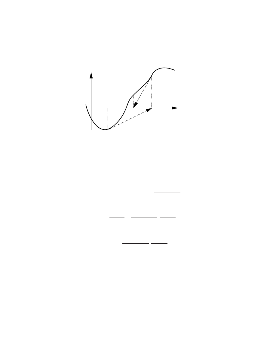
26
CHAPTER
3.
SOL
VING
NONLINEAR
EQUA
TIONS
until (hopefully) we obtain a solution that is suciently accurate. The geometrical interpretation
of the method is shown below.
f
(
x)
x
x
( 2 )
x
( 1 )
x
( 0 )
The function
f
at point
x
(0)
is approximated by a straight line which is tangent to
f
with slope
f
0
(
x
(0)
). The intersection of this line with the
x
-axis gives
x
(1)
, the function at
x
(1)
is approximated
by a tangent straight line which intersects the
x
-axis at
x
(2)
, etc.
3.1.2 Quadratic convergence
We now show that, once the solution is near the exact value
x
=
x
opt
, the Newton-Raphson method
converges quadratically. Let
x
(
j
)
indicate the solution at the
j
th
iteration. Consider the Taylor
series expansion
f
(
x
opt
) = 0
f
(
x
(
j
)
) + (
x
opt
;
x
(
j
)
)
f
0
(
x
(
j
)
) + (
x
opt
;
x
(
j
)
)
2
2
f
00
(
x
(
j
)
)
:
If
f
0
(
x
(
j
)
)
6
= 0, divide by
f
0
(
x
(
j
)
),
x
(
j
)
;
x
opt
f
(
x
(
j
)
)
f
0
(
x
(
j
)
) +
(
x
opt
;
x
(
j
)
)
2
2
f
0
0
(
x
(
j
)
)
f
0
(
x
(
j
)
)
:
Combining this with the Newton-Raphson formula (3.2) leads to
x
(
j
+1)
;
x
opt
(
x
(
j
)
;
x
opt
)
2
2
f
00
(
x
(
j
)
)
f
0
(
x
(
j
)
)
:
(3.3)
Dening the error at iteration
j
as
(
j
)
=
x
(
j
)
;
x
opt
, the error at the iteration
j
+ 1 is related to
the error at the iteration
j
by
(
j
+1)
1
2
f
00
(
x
(
j
)
)
f
0
(
x
(
j
)
)
(
j
)
2
:
That is, convergence is quadratic.
Note that convergence is guaranteed only if the initial guess is fairly close to the exact root
otherwise, the neglected higher-order terms dominate the above expression and we may encouter
divergence. If
f
0
is near zero at the root, we will also have problems.

3.1.
THE
NEWTON-RAPHSON
METHOD
F
OR
NONLINEAR
R
OOT
FINDING
27
3.1.3 Multivariable case|systems of nonlinear equations
A system of
n
nonlinear equations in
n
unknowns can be written in the general form:
f
i
(
x
1
x
2
:::x
n
) = 0
for
i
= 1
2
:::n
or, more compactly, as
f
(
x
) =
0
. As usual, subscripts denote vector components and boldface
denotes whole vectors. Generalization of the Newton-Raphson method to such systems is achieved
by using the multi-dimensional Taylor series expansion:
f
i
(
x
1
x
2
:::x
n
) =
f
i
(
x
(0)
1
x
(0)
2
:::x
(0)
n
) + (
x
1
;
x
(0)
1
)
@f
i
@x
1
x
=
x
(0)
+(
x
2
;
x
(0)
2
)
@f
i
@x
2
x
=
x
(0)
+
:::
=
f
i
(
x
(0)
1
x
(0)
2
:::x
(0)
n
) +
n
X
j
=1
(
x
j
;
x
(0)
j
)
@f
i
@x
j
x
=
x
(0)
+
:::
where, as in the previous section, superscripts denote iteration number. Thus, for example, the
components of the initial guess vector
x
(0)
are
x
(0)
i
for
i
= 1
2
:::n
. Let
x
(1)
be the solution of the
above equation with only the linear terms retained and with
f
i
(
x
1
x
2
:::x
n
) set to zero as desired.
Then
n
X
j
=1
@f
i
@x
j
x
=
x
(0)
|
{z
}
a
(0)
ij
(
x
(1)
j
;
x
(0)
j
)
|
{z
}
h
(1)
j
=
;
f
i
(
x
(0)
)
for
i
= 1
2
:::n:
(3.4)
Equation (3.4) constitutes
n
linear equations for the
n
components of
h
(1)
=
x
(1)
;
x
(0)
, which may
be considered as the desired update to
x
(0)
. In matrix notation, we have
A
(0)
h
(1)
=
;
f
(
x
(0)
)
where
a
(0)
ij
=
@f
i
@x
j
x
=
x
(0)
:
Note that the elemenets of the Jacobian matrix
A
(0)
are evaluated at
x
=
x
(0)
. The solution at the
rst iteration,
x
(1)
, is obtained from
x
(1)
=
x
(0)
+
h
(1)
:
Successive approximations are obtained from
A
(
k
)
h
(
k
+1)
=
;
f
(
x
(
k
)
)
x
(
k
+1)
=
x
(
k
)
+
h
(
k
+1)
where
a
(
k
)
ij
=
@f
i
@x
j
x
=
x
(k )
:
Note that the elements of the Jacobian matrix
A
(
k
)
are evaluated at
x
=
x
(
k
)
.
As an example, consider the nonlinear system of equations
f
(
x
) =
x
21
+ 3 cos
x
2
;
1
x
2
+ 2 sin
x
1
;
2
= 0
:
The Jacobian matrix is given by
A
(
k
)
=
0
B
@
@f
1
@x
1
@f
1
@x
2
@f
2
@x
1
@f
2
@x
2
1
C
A
x
=
x
(k )
=
2
x
(
k
)
1
;
3 sin
x
(
k
)
2
2 cos
x
(
k
)
1
1
!
:

28
CHAPTER
3.
SOL
VING
NONLINEAR
EQUA
TIONS
Let the initial guess be:
x
(0)
=
0
@
x
(0)
1
x
(0)
2
1
A
:
The function
f
and Jacobian
A
are rst evaluated at
x
=
x
(0)
. Next, the following system of
equations is solved for
h
(1)
A
(0)
h
(1)
=
;
f
(
x
(0)
)
:
We then update
x
according to
x
(1)
=
x
(0)
+
h
(1)
:
The function
f
and Jacobian
A
are then evaluated at
x
=
x
(1)
, and we solve
A
(1)
h
(2)
=
;
f
(
x
(1)
)
x
(2)
=
x
(1)
+
h
(2)
:
The process continues in an iterative fashion until convergence. A numerical solution to this example
nonlinear system is found in the following sections.
3.1.4 Matlab implementation
The following code is a modular Matlab implementation of the Newton-Raphson method. By using
modular programming style, we are most easily able to adapt segments of code written here for later
use on dierent nonlinear systems.
% newt.m
% Given an initial guess for the solution x and the auxiliary functions
% compute_f.m and compute_A.m to compute a function and the corresponding
% Jacobian, solve a nonlinear system using Newton-Raphson. Note that f may
% be a scalar function or a system of nonlinear functions of any dimension.
res=1 i=1
while (res>1e-10)
f=compute_f(x) A=compute_A(x)
% Compute function and Jacobian
res=norm(f)
% Compute residual
x_save(i,:)=x'
% Save x, f, and the residual
f_save(i,:)=f' res_save(i,1)=res
x=x-(A\f)
% Solve system for next x
i=i+1
% Increment index
end
evals=i-1
% end newt.m
The auxiliary functions (listed below) are written as functions rather than as simple Matlab scripts,
and all variables are passed in as arguments and pass back out via the function calls. Such hand-
shaking between subprograms eases debugging considerably when your programs become large.

3.1.
THE
NEWTON-RAPHSON
METHOD
F
OR
NONLINEAR
R
OOT
FINDING
29
function f] = compute_f(x)
f=x(1)*x(1)+3*cos(x(2))-1
% Evaluate the function f(x).
x(2)+2*sin(x(1))-2
]
% end function compute_f.m
function A] = compute_A(x)
A= 2*x(1)
-3*sin(x(2))
% Evaluate the Jacobian A
2*cos(x(1))
1
]
% of the function in compute_f
% end function compute_A.m
To prevent confusion with other cases presented in these notes, these case-specic functions are
stored at the class web site as
compute f.m.0
and
compute A.m.0
, and must be saved as
compute f.m
and
compute A.m
before the test code in the following section will run.
3.1.5 Dependence of Newton-Raphson on a good initial guess
The following code tests our implementation of the Newton-Raphson algorithm.
% test_newt.m
% Tests Newton's algorithm for nonlinear root finding.
% First, provide a sufficiently accurate initial guess for the root
clear format long x=init_x
% Find the root with Newton-Raphson and print the convergence
newt, x_save, res_save
% end test_newt.m
function x] = init_x
x=0 1]
% Initial guess for x
% end function init_x.m
As before, the case-specic function to compute the initial guess is stored at the class web site as
init x.m.0
, and must be saved as
init x.m
before the test code will run.
Typical results when applying the Newton-Raphson approach to solve a nonlinear system of
equations are shown below. It is seen that a \good" (lucky?) choice of initial conditions will converge
very rapidly to the solution with this scheme. A poor choice will not converge smoothly, and may not
converge at all|this is a major drawback to the Newton-Raphson approach. As nonlinear systems
do not necessarily have unique solutions, the nal root to which the system converges is dependent
on the choice of initial conditions. It is apparent in the results shown that, in this example, the
solution is not unique.

30
CHAPTER
3.
SOL
VING
NONLINEAR
EQUA
TIONS
A good initial guess
iteration
x
1
x
2
residual
1
0.0000
1.0000
1.17708342963828
2
0.3770
1.2460
0.10116915143065
3
0.3689
1.2788
0.00043489424427
4
0.3690
1.2787
0.00000000250477
5
0.3690
1.2787
0.00000000000000
A poor initial guess
iteration
x
1
x
2
1
0.00
-1.00
2
1.62
-1.25
3
-0.11
-0.18
4
2.42
-2.82
5
1.57
-0.60
6
-0.01
0.00
7
553.55
-1105.01
8
279.87
443.99
9
143.16
-261.08
10
72.58
34.77
11
36.75
-65.29
...
...
...
23
-1.82
4.39
24
-1.79
3.96
25
-1.74
3.97
26
-1.74
3.97
3.2 Bracketing approaches for scalar root nding
It was shown in the previous section that the Newton-Raphson technique is very ecient for nding
the solution of both scalar nonlinear equations of the form
f
(
x
) = 0 and multivariable nonlinear
systems of equations of the form
f
(
x
) =
0
when good initial guesses are available. Unfortunately,
good initial guesses are not always readily available. When they are not, it is desirable to seek
the roots of such equations by more pedestrian means which guarantee success. The techniques we
will present in this section, though they can not achieve quadratic convergence, are guaranteed to
converge to a solution of a scalar nonlinear equation so long as:
a) the function is continuous, and
b) an initial bracketing pair may be found.
They also have the added benet that they are based on function evaluations alone (i.e., you don't
need to write
compute A.m
), which makes them simple to implement. Unfortunately, these tech-
niques are based on a bracketing principle that does not extend readily to multi-dimensional func-
tions.
3.2.1 Bracketing a root
The class of scalar nonlinear functions we will consider are continuous. Our rst task is to nd a
pair of values for
x
which bracket the minimum, i.e., we want to nd an
x
(lower)
and an
x
(upper)
such that
f
(
x
(lower)
) and
f
(
x
(upper)
) have opposite signs. This may often be done by hand with a
minor amount of trial and error. At times, however, it is convenient to have an automatic procedure
to nd such a bracketing pair. For example, for functions which have opposite sign for suciently
large and small arguments, a simple approach is to start with an initial guess for the bracket and
then geometrically increase the distance between these points until a bracketing pair is found. This
may be implemented with the following codes (or variants thereof):

3.2.
BRA
CKETING
APPR
O
A
CHES
F
OR
SCALAR
R
OOT
FINDING
31
function x_lower,x_upper] = find_brack
x_lower,x_upper] = init_brack
while compute_f(x_lower) * compute_f(x_upper) > 0
interval=x_upper-x_lower
x_upper =x_upper+0.5*interval x_lower =x_lower-0.5*interval
end
% end function find_brack.m
The auxiliary functions used by this code may be written as
function x_lower,x_upper] = init_brack
x_lower=-1
x_upper=1
% Initialize a guess for the bracket.
% end function init_brack.m
function f] = compute_f(x)
f=x^3 + x^2 - 20*x + 50
% Evaluate the function f(x).
% end function compute_f.m
To prevent confusion with other cases presented in these notes, these case-specic functions are
stored at the class web site as
init brack.m.1
and
compute f.m.1
.
3.2.2 Rening the bracket - bisection
Once a bracketing pair is found, the task that remains is simply to rene this bracket until a desired
degree of precision is obtained. The most straightforward approach is to repeatedly chop the interval
in half, keeping those two values of
x
that bracket the root. The convergence of such an algorithm
is linear at each iteration, the bounds on the solution are reduced by exactly a factor of 2.
The bisection algorithm may be implemented with the following code:
% bisection.m
f_lower=compute_f(x_lower) f_upper=compute_f(x_upper)
evals=2
interval=x_upper-x_lower
i=1
while interval > x_tol
x = (x_upper + x_lower)/2
f = compute_f(x)
evals=evals+1
res_save(i,1)=norm(f)
plot(x,f,'ko')
if f_lower*f < 0
x_upper = x
f_upper = f
else
x_lower = x
f_lower = f
end
interval=interval/2
i=i+1 pause
end
x = (x_upper + x_lower)/2
% end bisection.m

32
CHAPTER
3.
SOL
VING
NONLINEAR
EQUA
TIONS
3.2.3 Rening the bracket - false position
A technique that is usually slightly faster than the bisection technique, but that retains the safety
of maintaining and rening a bracketing pair, is to compute each new point by a numerical approx-
imation to the Newton-Raphson formula (3.2) such that
x
(new)
=
x
(lower)
;
f
(
x
(lower)
)
f=x
(3.5)
where the quantity
f=x
is a simple dierence approximation to the slope of the function
f
f
x
=
f
(
x
(upper)
)
;
f
(
x
(lower)
)
x
(upper)
;
x
(lower)
:
As shown in class, this approach sometimes stalls, so it is useful to put in an ad hoc check to keep
the progress moving.
% false_pos.m
f_lower=compute_f(x_lower) f_upper=compute_f(x_upper)
evals=2
interval=x_upper-x_lower
i=1
while interval > x_tol
fprime = (f_upper-f_lower)/interval
x = x_lower - f_lower / fprime
% Ad hoc check: stick with bisection technique if updates
% provided by false position technique are too small.
tol1 = interval/10
if ((x-x_lower) < tol1 | (x_upper-x) < tol1)
x = (x_lower+x_upper)/2
end
f = compute_f(x) evals = evals+1
res_save(i,1)=norm(f)
plot(x_lower x_upper],f_lower f_upper],'k--',x,f,'ko')
if f_lower*f < 0
x_upper = x
f_upper = f
else
x_lower = x
f_lower = f
end
interval=x_upper-x_lower
i=i+1
pause
end
x = (x_upper + x_lower)/2
% end false_pos.m

3.2.
BRA
CKETING
APPR
O
A
CHES
F
OR
SCALAR
R
OOT
FINDING
33
3.2.4 Testing the bracketing algorithms
The following code tests the bracketing algorithms for scalar nonlinear rootnding and compares
with the Newton-Raphson algorithm. Convergence of the false position algorithm is usually found
to be faster than bisection, and both are safer (and slower) than Newton-Raphson. Don't forget
to update
init x.m
and
compute A.m
appropriately (i.e., with
init x.m.1
and
compute A.m.1
) in
order to get Newton-Raphson to work. You might have to ddle with
init x.m
in order to obtain
convergence of the Newton-Raphson algorithm.
% test_brack.m
% Tests the bisection, false position, and Newton routines for
% finding the root of a scalar nonlinear function.
% First, compute a bracket of the root.
clear x_lower,x_upper] = find_brack
% Prepare to make some plots of the function on this interval
xx=x_lower : (x_upper-x_lower)/100 : x_upper]
for i=1:101, yy(i)=compute_f(xx(i)) end
x1=x_lower x_upper] y1=0 0]
x_tol = 0.0001
% Set tolerance desired for x.
x_lower_save=x_lower x_upper_save=x_upper
fprintf('\n Now testing the bisection algorithm.\n')
figure(1) clf plot(xx,yy,'k-',x1,y1,'b-') hold on grid
title('Convergence of the bisection routine')
bisection
evals, hold off
fprintf(' Now testing the false position algorithm.\n')
figure(2) clf plot(xx,yy,'k-',x1,y1,'b-') hold on grid
title('Convergence of false position routine')
x_lower=x_lower_save
x_upper=x_upper_save
false_pos
evals, hold off
fprintf(' Now testing the Newton-Raphson algorithm.\n')
figure(3) clf plot(xx,yy,'k-') hold on grid
title('Convergence of the Newton-Raphson routine')
x=init_x
newt
% Finally, an extra bit of plotting stuff to show what happens:
x_lower_t=min(x_save) x_upper_t=max(x_save)
xx=x_lower_t : (x_upper_t-x_lower_t)/100 : x_upper_t]
for i=1:101, yy(i)=compute_f(xx(i)) end
plot(xx,yy,'k-',x_save(1),f_save(1),'ko') pause
for i=1:size(x_save)-1

34
plot(x_save(i) x_save(i+1)],f_save(i) 0],'k--', ...
x_save(i+1),f_save(i+1),'ko')
pause
end
evals, hold off
% end test_brack.m

Chapter
4
Interpolation
One often encounters the problem of constructing a smooth curve which passes through discrete data
points. This situation arises when developing dierentiation and integration strategies, as we will
discuss in the following chapters, as well as when simply estimating the value of a function between
known values. In this handout, we will present two techniques for this procedure: polynomial
(Lagrange) interpolation and cubic spline interpolation.
Note that the process of interpolation passes a curve exactly through each data point. This
is sometimes exactly what is desired. However, if the data is from an experiment and has any
appreciable amount of uncertainty, it is best to use a least-squares technique to t a low-order curve
in the general vicinity of several data points. This technique minimizes a weighted sum of the
square distance from each data points to this curve without forcing the curve to pass through each
data point individually. Such an approach generally produces a much smoother curve (and a more
physically-meaningful result) when the measured data is noisy.
4.1 Lagrange interpolation
Suppose we have a set of
n
+ 1 data points
f
x
i
y
i
g
. The process of Lagrange interpolation involves
simply tting an
n
'th degree polynomial (i.e., a polynomial with
n
+ 1 degrees of freedom) exactly
through this data. There are two ways of accomplishing this: solving a system of
n
+1 simultaneous
equations for the
n
+ 1 coecients of this polynomial, and constructing the polynomial directly in
factored form. We will present both of these techniques.
4.1.1 Solving
n
+
1
equations for the
n
+
1
coecients
Consider the polynomial
P
(
x
) =
a
o
+
a
1
x
+
a
2
x
2
+
:::
+
a
n
x
n
:
At each point
x
i
, this polynomial must take the value
y
i
, i.e.,
y
i
=
P
(
x
i
) =
a
o
+
a
1
x
i
+
a
2
x
2
i
+
:::
+
a
n
x
ni
for
i
= 0
1
2
::: n:
35

36
CHAPTER
4.
INTERPOLA
TION
In matrix form, we may write this system as
0
B
B
B
@
1
x
0
x
20
x
n
0
1
x
1
x
21
x
n
1
... ... ... ... ...
1
x
n
x
2
n
x
nn
1
C
C
C
A
|
{z
}
V
0
B
B
B
@
a
0
a
1
...
a
n
1
C
C
C
A
|
{z
}
a
=
0
B
B
B
@
y
0
y
1
...
y
n
1
C
C
C
A
|
{z
}
y
:
This system is of the form
V
a
=
y
, where
V
is commonly referred to as Vandermonde's matrix, and
may be solved for the vector
a
containing the coecients
a
i
of the desired polynomial. Unfortunately,
Vandermonde's matrix is usually quite poorly conditioned, and thus this technique of nding an
interpolating polynomial is unreliable at best.
4.1.2 Constructing the polynomial directly
Consider the
n
'th degree polynomial given by the factored expression
L
(
x
) =
(
x
;
x
0
)(
x
;
x
1
)
(
x
;
x
;
1
)(
x
;
x
+1
)
(
x
;
x
n
) =
n
Y
i=0
i6=
(
x
;
x
i
)
where
is a constant yet to be determined. This expression (by construction) is equal to zero if
x
is equal to any of the data points except
x
. In other words,
L
(
x
i
) = 0 for
i
6
=
. Choosing
to
normalize this polynomial at
x
=
x
, we dene
=
2
6
4
n
Y
i=0
i6=
(
x
;
x
i
)
3
7
5
;
1
which results in the very useful relationship
L
(
x
i
) =
i
=
(
1
i
=
0
i
6
=
:
Scaling this result, the polynomial
y
L
(
x
) (no summation implied) passes through zero at every
data point
x
=
x
i
except at
x
=
x
, where it has the value
y
. Finally, a linear combination of
n
+1
of these polynomials
P
(
x
) =
n
X
k
=0
y
k
L
k
(
x
)
provides an
n
'th degree polynomial which exactly passes through all of the data points, by construc-
tion.
A code which implements this constructive technique to determine the interpolating polynomial
is given in the following subsection.
Unfortunately, high-order polynomials tend to wander wildly between the data points even if
the data appears to be fairly regular, as shown in Figure 4.1. Thus, Lagrange interpolation should
be thought of as dangerous for anything more than a few data points and avoided in favor of other
techniques, such as spline interpolation.
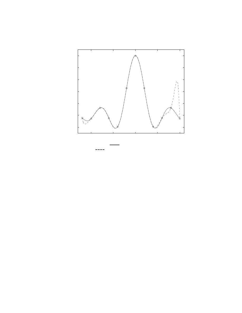
4.2.
CUBIC
SPLINE
INTERPOLA
TION
37
−10
−5
0
5
10
−0.2
0
0.2
0.4
0.6
0.8
1
Figure 4.1: The interpolation problem:
a continuous curve representing the function of interest
several points on this curve
the Lagrange interpolation of these points.
4.1.3 Matlab implementation
function p] = lagrange(x,x_data,y_data)
% Computes the Lagrange polynomial p(x) that passes through the given
% data {x_data,y_data}.
n=size(x_data,1)
p=0
for k=1:n
% For each data point {x_data(k),y_data(k)}
L=1
for i=1:k-1
L=L*(x-x_data(i))/(x_data(k)-x_data(i))
% Compute L_k
end
for i=k+1:n
L=L*(x-x_data(i))/(x_data(k)-x_data(i))
end
p = p + y_data(k) * L
% Add L_k's contribution to p(x)
end
% end lagrange.m
4.2 Cubic spline interpolation
Instead of forcing a high-order polynomial through the entire dataset (which often has the spurious
eect shown in Figure 4.1), we may instead construct a continuous, smooth, piecewise cubic function

38
CHAPTER
4.
INTERPOLA
TION
through the data. We will construct this function to be smooth in the sense of having continuous
rst and second derivatives at each data point. These conditions, together with the appropriate
conditions at each end, uniquely determine a piecewise cubic function through the data which is
usually reasonably smooth we will call this function the cubic spline interpolant.
Dening the interpolant in this manner is akin to deforming a thin piece of wood or metal to
pass over all of the data points plotted on a large block of wood and marked with thin nails. In
fact, the rst denition of the word \spline" in Webster's dictionary is \a thin wood or metal strip
used in building construction"|this is where the method takes its name. The elasticity equation
governing the deformation
f
of the spline is
f
0000
=
G
(4.1)
where
G
is a force localized near each nail (i.e., with a delta function) which is sucient to pass
the spline through the data. As
G
is nonzero only in the immediate vicinity of each nail, such a
spline takes an approximately piecewise cubic shape between the data points. Thus, between the
data points
, we have:
f
0000
= 0
f
000
=
C
1
f
0
0
=
C
1
x
+
C
2
f
0
=
C
1
2
x
2
+
C
2
x
+
C
3
and
f
=
C
1
6
x
3
+
C
2
2
x
2
+
C
3
x
+
C
4
:
4.2.1 Constructing the cubic spline interpolant
Let
f
i
(
x
) denote the cubic in the interval
x
i
x
x
i
+1
and let
f
(
x
) denote the collection of all the
cubics for the entire range
x
0
x
x
n
. As noted above,
f
00
i
varies linearly with
x
between each
data point. At each data point, by (4.1) with
G
being a linear combination of delta functions, we
have:
(a) continuity of the function
f
, i.e.,
f
i
;
1
(
x
i
) =
f
i
(
x
i
) =
f
(
x
i
) =
y
i
(b) continuity of the rst derivative
f
0
, i.e.,
f
0
i
;
1
(
x
i
) =
f
0
i
(
x
i
) =
f
0
(
x
i
)
and
(c) continuity of the second derivative
f
00
, i.e.,
f
00
i
;
1
(
x
i
) =
f
0
0
i
(
x
i
) =
f
00
(
x
i
)
:
We now describe a procedure to determine an
f
which satises conditions (a) and (c) by construction,
in a manner analogous to the construction of the Lagrange interpolant in
x
4.1.2, and which satises
condition (b) by setting up and solving the appropriate system of equations for the value of
f
00
at
each data point
x
i
.
To begin the constructive procedure for determining
f
, note that on each interval
x
i
x
x
i
+1
for
i
= 0
1
::: n
;
1, we may write a linear equation for
f
00
i
(
x
) as a function of its value at the
endpoints,
f
00
(
x
i
) and
f
00
(
x
i
+1
), which are (as yet) undetermined. The following form (which is
linear in
x
) ts the bill by construction:
f
00
i
(
x
) =
f
0
0
(
x
i
)
x
;
x
i
+1
x
i
;
x
i
+1
+
f
0
0
(
x
i
+1
)
x
;
x
i
x
i
+1
;
x
i
:
Note that this rst degree polynomial is in fact just a Lagrange interpolation of the two data
points
f
x
i
f
0
0
(
x
i
)
g
and
f
x
i
+1
f
00
(
x
i
+1
)
g
. By construction, condition (c) is satised. Integrating this
equation twice and dening $
i
=
x
i
+1
;
x
i
, it follows that
f
0
i
(
x
) =
;
f
00
(
x
i
)
2
(
x
i
+1
;
x
)
2
$
i
+
f
0
0
(
x
i
+1
)
2
(
x
;
x
i
)
2
$
i
+
C
1
:
f
i
(
x
) =
f
00
(
x
i
)
6
(
x
i
+1
;
x
)
3
$
i
+
f
00
(
x
i
+1
)
6
(
x
;
x
i
)
3
$
i
+
C
1
x
+
C
2
:

4.2.
CUBIC
SPLINE
INTERPOLA
TION
39
The undetermined constants of integration are obtained by matching the end conditions
f
i
(
x
i
) =
y
i
and
f
i
(
x
i
+1
) =
y
i
+1
:
A convenient way of constructing the linear and constant terms in the expression for
f
i
(
x
) in such
a way that the desired end conditions are met is by writing
f
i
(
x
) in the form
f
i
(
x
) =
f
00
(
x
i
)
6
(
x
i
+1
;
x
)
3
$
i
;
$
i
(
x
i
+1
;
x
)
+
f
00
(
x
i
+1
)
6
(
x
;
x
i
)
3
$
i
;
$
i
(
x
;
x
i
)
+
y
i
(
x
i
+1
;
x
)
$
i
+
y
i
+1
(
x
;
x
i
)
$
i
where
x
i
x
x
i
+1
:
(4.2)
By construction, condition (a) is satised. Finally, an expression for
f
0
i
(
x
) may now be found by
dierentiating this expression for
f
i
(
x
), which gives
f
0
i
(
x
) =
f
00
(
x
i
)
6
;
3(
x
i
+1
;
x
)
2
$
i
+ $
i
+
f
00
(
x
i
+1
)
6
3(
x
;
x
i
)
2
$
i
;
$
i
+
y
i
+1
$
i
;
y
i
$
i
:
The second derivative of
f
at each node,
f
00
(
x
i
), is still undetermined. A system of equations from
which the
f
00
(
x
i
) may be found is obtained by imposing condition (b), which is achieved by setting
f
0
i
(
x
i
) =
f
0
i
;
1
(
x
i
)
for
i
= 1
2
::: n
;
1
:
Substituting appropriately from the above expression for
f
0
i
(
x
), noting that $
i
=
x
i
+1
;
x
i
, leads to
$
i
;
1
6
f
00
(
x
i
;
1
) + $
i
;
1
+ $
i
3
f
00
(
x
i
) + $
i
6
f
00
(
x
i
+1
) =
y
i
+1
;
y
i
$
i
;
y
i
;
y
i
;
1
$
i
;
1
(4.3)
for
i
= 1
2
::: n
;
1. This is a diagonally-dominant tridiagonal system of
n
;
1 equations for the
n
+ 1 unknowns
f
00
(
x
0
),
f
00
(
x
1
),
:::
,
f
00
(
x
n
). We nd the two remaining equations by prescribing
conditions on the interpolating function at each end. We will consider three types of end conditions:
Parabolic run-out:
f
00
(
x
0
) =
f
0
0
(
x
1
)
f
00
(
x
n
) =
f
0
0
(
x
n
;
1
)
(4.4)
Free run-out (also known as natural splines):
f
00
(
x
0
) = 0
f
00
(
x
n
) = 0
(4.5)
Periodic end-conditions:
f
00
(
x
0
) =
f
00
(
x
n
;
1
)
f
00
(
x
1
) =
f
00
(
x
n
)
(4.6)
Equation (4.3) may be taken together with equation (4.4), (4.5), or (4.6) (making the appropriate
choice for the end conditions depending upon the problem at hand) to give us
n
+1 equations for the
n
+ 1 unknowns
f
00
(
x
i
). This set of equations is then solved for the
f
00
(
x
i
), which thereby ensures
that condition (b) is satised. Once this system is solved for the
f
0
0
(
x
i
), the cubic spline interpolant
follows immediately from equation (4.2).
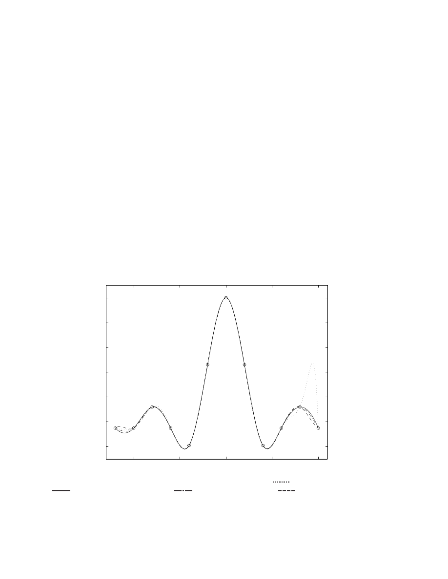
40
CHAPTER
4.
INTERPOLA
TION
x
i
;
12
;
10
;
8
;
6
;
4
;
2 0
2
4
6
8
10
y
i
;
0
:
05
;
0
:
05 0
:
12
;
0
:
05
;
0
:
19 0
:
46 1 0
:
46
;
0
:
19
;
0
:
05 0
:
12
;
0
:
05
Table 4.1: Data points from which we want to reproduce (via interpolation) a continuous function.
These data points all lie near the familiar curve generated by the function sin(
x
)
=x
.
Note that, when equation (4.3) is taken together with parabolic or free run-out at the ends,
a tridiagonal system results which can be solved eciently with the Thomas algorithm. When
equation (4.3) is taken together periodic end conditions, a tridiagonal circulant system (which is
not diagonally dominant) results. A code which solves these systems to determine the cubic spline
interpolation with any of the above three end-conditions is given in the following subsection.
The results of applying the cubic spline interpolation formula to the set of data given in Table
4.1 is shown in Figure 4.2. All three end conditions on the cubic spline do reasonably well, but the
Lagrange interpolation is again spurious. Note that applying periodic end conditions on the spline
in this case (which is not periodic) leads to a non-physical \wiggle" in the interpolated curve near
the left end in general, the periodic end conditions should be reserved for those cases for which
the function being interpolated is indeed periodic. The parabolic run-out simply places a parabola
between
x
0
and
x
1
, whereas the free run-out tapers the curvature down to zero near
x
0
. Both end
conditions provide reasonably smooth interpolations.
−10
−5
0
5
10
−0.2
0
0.2
0.4
0.6
0.8
1
Figure 4.2: Various interpolations of the data of Table 1:
data
Lagrange interpolation
cubic spline (parabolic run-out)
cubic spline (free run-out)
cubic spline (periodic).

4.2.
CUBIC
SPLINE
INTERPOLA
TION
41
4.2.2 Matlab implementation
% spline_setup.m
% Determines the quantity g=f'' for constructing a cubic spline
% interpolation of a function. Note that this algorithm calls
% thomas.m, which was developed earlier in the course, and assumes
% the x_data is already sorted in ascending order.
% Compute the size of the problem.
n=size(x_data,1)
% Set up the delta_i = x_(i+1)-x_i for i=1:n-1.
delta(1:n-1)=x_data(2:n)-x_data(1:n-1)
% Set up and solve a tridiagonal system for the g at each data point.
for i=2:n-1
a(i)=delta(i-1)/6
b(i)=(delta(i-1)+delta(i))/3
c(i)=delta(i)/6
g(i)=(y_data(i+1)-y_data(i))/delta(i) -...
(y_data(i)-y_data(i-1))/delta(i-1)
end
if end_conditions==1
% Parabolic run-out
b(1)=1 c(1)=-1 g(1)=0
b(n)=1 a(n)=-1 g(n)=0
thomas
% <--- solve system
elseif end_conditions==2
% Free run-out ("natural" spline)
b(1)=1 c(1)=0
g(1)=0
b(n)=1 a(n)=0
g(n)=0
thomas
% <--- solve system
elseif end_conditions==3
% Periodic end conditions
a(1)=-1 b(1)=0 c(1)=1
g(1)=0
a(n)=-1 b(n)=0 c(n)=1
g(n)=0
% Note: the following is an inefficient way to solve this circulant
% (but NOT diagonally dominant!) system via full-blown Gaussian
% elimination.
A = diag(a(2:n),-1) + diag(b,0) + diag(c(1:n-1),1)
A(1,n)=a(1) A(n,1)=c(1)
g=A\g' % <--- solve system
end
% end spline_setup.m
-----------------------------------------------------------------

42
CHAPTER
4.
INTERPOLA
TION
function f] = spline_interp(x,x_data,y_data,g,delta)
n=size(x_data,1)
% Find that value of i such that x_data(i) <= x <= x_data(i+1)
for i=1:n-1
if x_data(i+1) > x, break, end
end
% compute the cubic spline approximation of the function.
f=g(i) /6 *((x_data(i+1)-x)^3/delta(i)-delta(i)*(x_data(i+1)-x))+...
g(i+1)/6 *((x - x_data(i))^3/delta(i)-delta(i)*(x - x_data(i)))+...
(y_data(i)*(x_data(i+1)-x) + y_data(i+1)*(x-x_data(i))) / delta(i)
% end spline_interp.m
-----------------------------------------------------------------
% test_interp.m
clear clf
x_data, y_data]=input_data
plot(x_data,y_data,'ko') axis(-13 11 -0.3 1.1])
hold on pause
x_lower=min(x_data) x_upper=max(x_data)
xx=x_lower : (x_upper-x_lower)/200 : x_upper]
for i=1:201
ylagrange(i)=lagrange(xx(i),x_data,y_data)
end
plot(xx,ylagrange,'b:') pause
for end_conditions=1:3
% Set the end conditions you want to try here.
spline_setup
for i=1:201
y_spline(i)=spline_interp(xx(i),x_data,y_data,g,delta)
end
plot(xx,y_spline) pause
end
% end test_interp.m
-----------------------------------------------------------------
function x_data,y_data] = input_data
x_data=-12:2:10]'
y_data=sin(x_data+eps)./(x_data+eps)
% end input_data.m

4.2.
CUBIC
SPLINE
INTERPOLA
TION
43
4.2.3 Tension splines
For some special cases, cubic splines aren't even smooth enough. In such cases, it is helpful to put
\tension" on the spline to straighten out the curvature between the \nails" (datapoints). In the
limit of large tension, the interpolant becomes almost piecewise linear.
Tensioned splines obey the dierential equation:
f
0000
;
2
f
0
0
=
G
where
is the tension of the spline. This leads to the following relationships between the data
points:
!
f
00
;
2
f
]
0
0
= 0
!
f
00
;
2
f
]
0
=
C
1
!
f
00
;
2
f
] =
C
1
x
+
C
2
:
Solving the ODE on the right leads to an equation of the form
f
=
;
;
2
(
C
1
x
+
C
2
) +
C
3
e
;
x
+
C
4
e
x
:
Proceeding with a constructive process to satisfy condition (a) as discussed in
x
4.2.1, we assemble
the linear and constant terms of
f
00
;
2
f
such that
f
0
0
i
(
x
)
;
2
f
i
(
x
)
=
f
00
i
(
x
i
)
;
2
y
i
x
;
x
i
+1
x
i
;
x
i
+1
+
f
00
i
(
x
i
+1
)
;
2
y
i
+1
x
;
x
i
x
i
+1
;
x
i
:
Similarly, we assemble the exponential terms in the solution of this ODE for
f
in a constructive
manner such that condition (c) is satised. Rewriting the exponentials as sinh functions, the desired
solution may be written
f
i
(
x
) =
;
;
2
n
f
0
0
(
x
i
)
;
2
y
i
x
i
+1
;
x
$
i
+
f
00
(
x
i
+1
)
;
2
y
i
+1
x
;
x
i
$
i
;
f
00
(
x
i
)sinh
(
x
i
+1
;
x
)
sinh
$
i
;
f
0
0
(
x
i
+1
)sinh
(
x
;
x
i
)
sinh
$
i
o
where
x
i
x
x
i
+1
:
(4.7)
Dierentiating once and appling condition (b) leads to the tridiagonal system:
1
$
i
;
1
;
sinh
$
i
;
1
f
00
(
x
i
;
1
)
2
;
1
$
i
;
1
;
cosh
$
i
;
1
sinh
$
i
;
1
+ 1$
i
;
cosh
$
i
sinh
$
i
f
00
(
x
i
)
2
+
1
$
i
;
sinh
$
i
f
0
0
(
x
i
+1
)
2
=
y
i
+1
;
y
i
$
i
;
y
i
;
y
i
;
1
$
i
;
1
:
(4.8)
The tridiagonal system (4.8) can be set up and solved exactly as was done with (4.3), even though
the coecients have a slightly more complicated form. The tensioned-spline interpolant is then given
by (4.7).
4.2.4 B-splines
It is interesting to note that we may write the cubic spline interpolant in a similar form to how we
constructed the Lagrange interpolant, that is,
f
(
x
) =
n
X
=0
y
b
(
x
)

44
where the
b
(
x
) correspond to the various cubic spline interpolations of the Kronecker deltas such
that
b
(
x
i
) =
i
, as discussed in
x
4.1.2 for the functions
L
(
x
). The
b
(
x
) in this representation
are referred to as the basis functions, and are found to have
localized support
(in other words,
b
(
x
)
!
0 for large
j
x
;
x
j
).
By relaxing some of the continuity constraints, we may conne each of the basis functions to
have
compact support
(in other words, we can set
b
(
x
) = 0 exactly for
j
x
;
x
j
> R
for some
R
). With such functions, it is easier both to compute the interpolations themselves and to project
the interpolated function onto a dierent mesh of gridpoints. The industry of computer animation
makes heavy use of ecient algorithms for this type of interpolation extended to three-dimensional
problems.

Chapter
5
Minimization
5.0 Motivation
It is often the case that one needs to minimize a scalar function of one or several variables. Three
cases of particular interest which motivate the present chapter are described here.
5.0.1 Solution of large linear systems of equations
Consider the
n
n
problem
A
x
=
b
, where
n
is so large that an
O
(
n
3
) algorithm such as
Gaussian elimination is out of the question, and the problem can not be put into such a form that
A
has a banded structure. In such cases, it is sometimes useful to construct a function
J
(
x
) such
that, once (approximately) minimized via an iterative technique, the desired condition
A
x
=
b
is
(approximately) satised. If
A
is symmetric positive denite (i.e., if
a
kj
=
a
jk
and all eigenvalues
of
A
are positive) then we can accomplish this by dening
J
(
x
) = 12
x
T
A
x
;
b
T
x
= 12
x
i
a
ij
x
j
;
b
i
x
i
:
Requiring that
A
be symmetric positive denite insures that
J
!
1
for
j
x
j
!
1
in all directions
and thus that a minimum point indeed exists. (We will extend this approach to more general
problems at the end of this chapter.) Dierentiating
J
with respect to an arbitrary component of
x
, we nd that
@
J
@x
k
= 12 (
ik
a
ij
x
j
+
x
i
a
ij
jk
)
;
b
i
ik
=
a
kj
x
j
;
b
k
:
The unique minimum of
J
(
x
) is characterized by
@
J
@x
k
=
a
kj
x
j
;
b
k
= 0
or
r
J
=
A
x
;
b
=
0
:
Thus, solution of large linear systems of the form
A
x
=
b
(where
A
is symmetric positive denite)
may be found by minimization of
J
(
x
).
5.0.2 Solution of nonlinear systems of equations
Recall from
x
3.1 that the Newton-Raphson method was an eective technique to nd the root (when
one exists) of a nonlinear system of equations
f
(
x
) =
0
when a suciently-accurate initial guess is
45

46
CHAPTER
5.
MINIMIZA
TION
available. When such a guess is not available, an alternative technique is to examine the square of
the norm of the vector
f
:
J
(
x
) = !
f
(
x
)]
T
f
(
x
)
Note that this quantity is never negative, so any point
x
for which
f
(
x
) =
0
minimizes
J
(
x
). Thus,
seeking a minimum of this
J
(
x
) with respect to
x
might result in an
x
such that
f
(
x
) =
0
. However,
there are quite likely many minimum points of
J
(
x
) (at which
r
J
=
0
), only some of which (if any!)
will correspond to
f
(
x
) =
0
. Root nding in systems of nonlinear equations is very dicult|though
this method has signicant drawbacks, variants of this method are really about the best one can do
when one doesn't have a good initial guess for the solution.
5.0.3 Optimization and control of dynamic systems
In control and optimization problems, one can often represent the desired objective mathematically
as a \cost function" to be minimized. When the cost function is formulated properly, its minimization
with respect to the control parameters results in an eectively-controlled dynamic system. Such cost
functions may often be put in the form
J
(
u
) =
x
T
Q
x
+
u
T
R
u
where
x
=
x
(
u
) is the state of the system and
u
is the control. The second term in the above
expression measures the amount of control used and the rst term is an observation of the property
of interest of the dynamic system which, in turn, is a function of the applied control. When the
control is both ecient (small in magnitude) and has the desired eect on the dynamic system, both
of these terms are small. Thus, minimization of this cost function with respect to
u
results in the
determination of an eective set of control parameters.
5.1 The Newton-Raphson method for nonquadratic mini-
mization
If a good initial guess is available (near the desired minimum point), minimization of
J
(
x
) can be
accomplished simply by applying the Newton-Raphson method developed previously to the gradient
of
J
(
x
), given by function
f
(
x
) =
r
J
, in order to nd the solution to the equation
f
(
x
) =
0
. This
works just as well for scalar or vector
x
, and converges quite rapidly. Recall from equation (3.4)
that the Newton-Raphson method requires both evaluation of the function
f
(
x
), in this case taken
to be the gradient of
J
(
x
), and the Jacobian of
f
(
x
), given in this case by
a
(
k
)
ij
=
@f
i
@x
j
x
=
x
(k )
=
@
2
J
@x
i
@x
j
x
=
x
(k )
:
This matrix of second derivatives is referred to as the Hessian of the function
J
. Unfortunately,
for very large
N
, computation and storage of the Hessian matrix, which has
N
2
elements, can be
prohibitively expensive.

5.2.
BRA
CKETING
APPR
O
A
CHES
F
OR
MINIMIZA
TION
OF
SCALAR
FUNCTIONS
47
5.2 Bracketing approaches for minimization of scalar func-
tions
5.2.1 Bracketing a minimum
We now seek a reliable but pedestrian approach to a minimize scalar function
J
(
x
) when a good
initial guess for the minimum is not available. To do this, we begin with a \bracketing" approach
analogous to that which we used for nding the root of a nonlinear scalar equation. Recall from
x
3.2
that bracketing a root means nding a pair
f
x
(lower)
x
(upper)
g
for which
f
(
x
(lower)
) and
f
(
x
(upper)
)
have opposite signs (so a root must exist between
x
(lower)
and
x
(upper)
if the function is continuous
and bounded).
Analogously, bracketing a minimum means nding a triplet
f
x
1
x
2
x
3
g
with
x
2
between
x
1
and
x
3
and for which
J
(
x
2
)
<
J
(
x
1
) and
J
(
x
2
)
<
J
(
x
3
) (so a minimum must exist between
x
1
and
x
3
if the function is continuous and bounded). Such an initial bracketing triplet may often be found
by a minor amount of trial and error. At times, however, it is convenient to have an automatic
procedure to nd such a bracketing triplet. For example, for functions which are large and positive
for suciently large
j
x
j
, a simple approach is to start with an initial guess for the bracket and then
geometrically scale out each end until a bracketing triplet is found.
Matlab implementation
% find_triplet.m
% Initialize and expand a triplet until the minimum is bracketed.
% Should work if J -> inf as |x| -> inf.
x1,x2,x3] = init_triplet
J1=compute_J(x1) J2=compute_J(x2) J3=compute_J(x3)
while (J2>J1)
% Compute a new point x4 to the left of the triplet
x4=x1-2.0*(x2-x1) J4=compute_J(x4)
% Center new triplet on x1
x3=x2
J3=J2
x2=x1
J2=J1
x1=x4
J1=J4
end
while (J2>J3)
% Compute new point x4 to the right of the triplet
x4=x3+2.0*(x3-x2)
J4=compute_J(x4)
% Center new triplet on x3
x1=x2
J1=J2
x2=x3
J2=J3
x3=x4
J3=J4
end
% end find_triplet.m
Case-specic auxiliary functions are given below.
function J] = compute_J(x)
J=3*cos(x)-sin(2*x) + 0.1*x.^2 % compute function you are trying to minimize.
plot(x,J,'ko')
% plot a circle at the data point.
% end compute_J.m
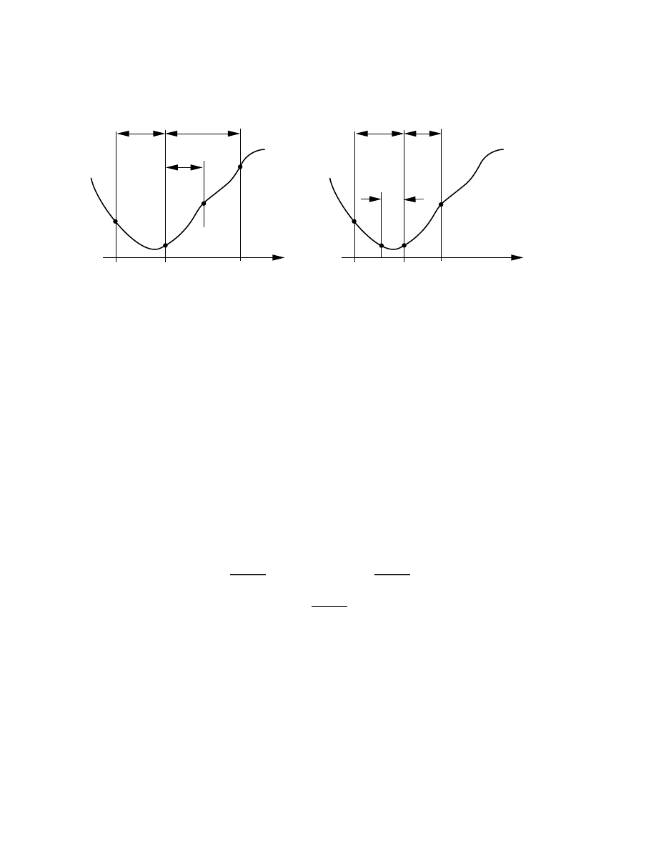
48
CHAPTER
5.
MINIMIZA
TION
J(x)
x
1
(k)
W
(k)
1
−W
(k)
Z
(k)
x
2
(k)
x
3
(k)
x
4
(k)
)
J(x)
x
3
(k+1)
W
(k+1)
1
−W
(k+1)
Z
(k+1)
x
2
(k+1)
x
1
(k+1)
x
4
(k+1)
k
'th iteration
(
k
+ 1)'th iteration
Figure 5.1: Naming of points used in golden section search procedure:
f
x
(
k
)
1
x
(
k
)
2
x
(
k
)
3
g
is referred
to as the bracketing triplet at iteration
k
, where
x
(
k
)
2
is between
x
(
k
)
1
and
x
(
k
)
3
and
x
(
k
)
2
is assumed
to be closer to
x
(
k
)
1
than it is to
x
(
k
)
3
. A new guess is made at point
x
(
k
)
4
and the bracket is rened
by retaining those three of the four points which maintain the tightest bracket. The reduction of
the interval continues at the following iterations in a self-similar fashion.
function x1,x2,x3] = init_triplet
x1=-5 x2=0 x3=5
% Initialize guess for the bracketing triplet
% end init_triplet.m
5.2.2 Rening the bracket - the golden section search
Once the minimum of the non-quadratic function is bracketed, all that remains to be done is to
rene these brackets. A simple algorithm to accomplish this, analogous to the bisection technique
developed for scalar root nding, is called the golden section search. As illustrated in Figure 5.1, let
W
be dened as the ratio of the smaller interval to the width of the bracketing triplet
f
x
1
x
2
x
3
g
such that
W
=
x
2
;
x
1
x
3
;
x
1
)
1
;
W
=
x
3
;
x
2
x
3
;
x
1
:
We now pick a new trial point
x
4
and dene
Z
=
x
4
;
x
2
x
3
;
x
1
)
x
4
=
x
2
+
Z
(
x
3
;
x
1
)
:
There are two possibilities:
if
J
(
x
4
)
>
J
(
x
2
), then
f
x
4
x
2
x
1
g
is a new bracketing triplet (as in Figure 5.1), and
if
J
(
x
4
)
<
J
(
x
2
), then
f
x
2
x
4
x
3
g
is a new bracketing triplet.
Minimizing the width of this new (rened) bracketing triplet in the worst case, we should take the
width of both of these triplets as identical, so that
W
+
Z
= 1
;
W
)
Z
= 1
;
2
W
(5.1)
If the same algorithm is used for the renement at each iteration
k
, then a self-similar situation
develops in which the ratio
W
is constant from one iteration to the next, i.e.,
W
(
k
)
=
W
(
k
+1)
. Note
that, in terms of the quantities at iteration
k
, we have either

5.2.
BRA
CKETING
APPR
O
A
CHES
F
OR
MINIMIZA
TION
OF
SCALAR
FUNCTIONS
49
W
k
+1
=
Z
(
k
)
=
(
W
(
k
)
+
Z
(
k
)
) if
f
x
(
k
)
4
x
(
k
)
2
x
(
k
)
1
g
is the new bracketing triplet, or
W
k
+1
=
Z
(
k
)
=
(1
;
W
(
k
)
) if
f
x
(
k
)
2
x
(
k
)
4
x
(
k
)
3
g
is the new bracketing triplet.
Dropping the superscripts on
W
and
Z
, which we assume to be independent of
k
, and inserting
(5.1), both of these conditions reduce to the relation
W
2
;
3
W
+ 1 = 0
which (because 0
< W <
1) implies that
W
= 3
;
p
5
2
0
:
381966
)
1
;
W
=
p
5
;
1
2
0
:
618034 and
Z
=
p
5
;
2
0
:
236068
:
These proportions are referred to as the golden section.
To summarize, the golden section algorithm takes an initial bracketing triplet
f
x
(0)
1
x
(0)
2
x
(0)
3
g
,
computes a new data point at
x
(0)
4
=
x
(0)
2
+
Z
(
x
(0)
3
;
x
(0)
1
) where
Z
= 0
:
236068, and then:
if
J
(
x
(0)
4
)
>
J
(
x
(0)
2
), the new triplet is
f
x
(1)
1
x
(1)
2
x
(1)
3
g
=
f
x
(0)
4
x
(0)
2
x
(0)
1
g
, or
if
J
(
x
(0)
4
)
<
J
(
x
(0)
2
), the new triplet is
f
x
(1)
1
x
(1)
2
x
(1)
3
g
=
f
x
(0)
2
x
(0)
4
x
(0)
3
g
.
The process continues on the new (rened) bracketing triplet in an iterative fashion until the desired
tolerance is reached such that
j
x
3
;
x
1
j
<
. Even if the initial bracketing triplet is not in the ratio
of the golden section, repeated application of this algorithm quickly brings the triplet into this ratio
as it is rened. Note that convergence is attained linearly: each bound on the minimum is 0.618034
times the previous bound. This is slightly slower than the convergence of the bisection algorithm
for nonlinear root-nding.
Matlab implementation
% golden.m
% Input assumes {x1,x2,x3} are a bracketing triple with function
% values {J1,J2,J3}. On output, x2 is the best guess of the minimum.
Z=sqrt(5)-2
% initialize the golden section ratio
if (abs(x2-x1) > abs(x2-x3))
% insure proper ordering
swap=x1 x1=x3 x3=swap
swap=J1 J1=J3 J3=swap
end
pause
while (abs(x3-x1) > x_tol)
x4 = x2 + Z*(x3-x1)
% compute and plot new point
J4 = compute_J(x4)
evals = evals+1
% Note that a couple of lines are commented out below because some
% of the data is already in the right place!
if (J4>J2)
x3=x1
J3=J1
% Center new triplet on x2
% x2=x2
J2=J2
x1=x4
J1=J4
else

50
CHAPTER
5.
MINIMIZA
TION
x1=x2
J1=J2
% Center new triplet on x4
x2=x4
J2=J4
% x3=x3
J3=J3
end
pause
end
% end golden.m
The implementation of the golden section search algorithm may be tested as follows:
% test_golden.m
% Tests the golden search routine
clear find_triplet
% Initialize a bracket of the minimum.
% Prepare to make some plots of the function over the width of the triplet
xx=x1 : (x3-x1)/100 : x3]
for i=1:101, yy(i)=compute_J(xx(i)) end
figure(1) clf plot(xx,yy,'k-') hold on grid
title('Convergence of the golden section search')
plot(x1,J1,'ko') plot(x2,J2,'ko') plot(x3,J3,'ko')
x_tol = 0.0001 % Set desired tolerance for x.
evals=0
% Reset a counter for tracking function evaluations.
golden hold off
x2, J2, evals
% end test_golden.m
5.2.3 Rening the bracket - inverse parabolic interpolation
Recall from
x
3.2.3 that, when a function
f
(
x
) is \locally linear" (meaning that its shape is well-
approximated by a linear function), the false position method is an ecient technique to nd the
root of the function based on function evaluations alone. The false position method is based on
the construction of successive linear interpolations of recent function evaluations, taking each new
estimate of the root of
f
(
x
) as that value of
x
for which the value of the linear interpolant is zero.
Analogously, when a function
J
(
x
) is \locally quadratic" (meaning that its shape is well-
approximated by a quadratic function), the minimum point of the function may be found via an
ecient technique based on function evaluations alone. At the heart of this technique is the con-
struction of successive quadratic interpolations based on recent function evaluations, taking each
new estimate of the minimum of
J
(
x
) as that value of
x
for which the value of the quadratic inter-
polant is minimum. For example, given data points
f
x
0
y
0
g
,
f
x
1
y
1
g
, and
f
x
2
y
2
g
, the quadratic
interpolant is given by the Lagrange interpolation formula
P
(
x
) =
y
0
(
x
;
x
1
)(
x
;
x
2
)
(
x
0
;
x
1
)(
x
0
;
x
2
) +
y
1
(
x
;
x
0
)(
x
;
x
2
)
(
x
1
;
x
0
)(
x
1
;
x
2
) +
y
2
(
x
;
x
0
)(
x
;
x
1
)
(
x
2
;
x
0
)(
x
2
;
x
1
)
as described in
x
4.1. Setting
dP
(
x
)
=dx
= 0 to nd the critical point of this quadratic yields
0 =
y
0
2
x
;
x
1
;
x
2
(
x
0
;
x
1
)(
x
0
;
x
2
) +
y
1
2
x
;
x
0
;
x
2
(
x
1
;
x
0
)(
x
1
;
x
2
) +
y
2
2
x
;
x
0
;
x
1
(
x
2
;
x
0
)(
x
2
;
x
1
)
:

5.2.
BRA
CKETING
APPR
O
A
CHES
F
OR
MINIMIZA
TION
OF
SCALAR
FUNCTIONS
51
Multiplying by (
x
0
;
x
1
)(
x
1
;
x
2
)(
x
2
;
x
0
) and then solving for
x
gives the desired value of
x
which
is a critical point of the interpolating quadratic:
x
= 12
y
0
(
x
1
+
x
2
)(
x
1
;
x
2
) +
y
1
(
x
0
+
x
2
)(
x
2
;
x
0
) +
y
2
(
x
0
+
x
1
)(
x
0
;
x
1
)
y
0
(
x
1
;
x
2
) +
y
1
(
x
2
;
x
0
) +
y
2
(
x
0
;
x
1
)
:
Note that the critical point found may either be a minimum point or a maximum point depending
on the relative orientation of the data, but will always maintain the bracketing triplet.
Matlab implementation
% inv_quad.m
% Finds the minimum or maximum of a function by repeatedly moving to the
% critical point of a quadratic interpolant of three recently-computed data points
% in an attempt to home in on the critical point of a nonquadratic function.
res=1 i=1
J1=compute_J(x1) J2=compute_J(x2) J3=compute_J(x3)
while (abs(x3-x1) > x_tol)
x4 = 0.5*(J1*(x2+x3)*(x2-x3)+ J2*(x3+x1)*(x3-x1)+ J3*(x1+x2)*(x1-x2))/...
(J1*(x2-x3)+ J2*(x3-x1)+ J3*(x1-x2))
% compute the critical point
% The following plotting stuff is done for demonstration purposes only.
x_lower=min(x1 x2 x3]) x_upper=max(x1 x2 x3])
xx=x_lower : (x_upper-x_lower)/200 : x_upper]
for i=1:201
J_lagrange(i)=lagrange(xx(i),x1 x2 x3],J1 J2 J3])
end
plot(xx,J_lagrange,'b-')
% plot a curve through the data
Jinterp=lagrange(x4,x1 x2 x3],J1 J2 J3]) % plot a * at the critical point
plot(x4,Jinterp,'r*')
% of the Lagrange interpolant.
pause
J4 = compute_J(x4)
% Compute function J at new point and the proceed as with
evals = evals+1
% the golden section search.
% Note that a couple of lines are commented out below because some
% of the data is already in the right place!
if (J4>J2)
x3=x1
J3=J1
% Center new triplet on x2
% x2=x2
J2=J2
x1=x4
J1=J4
else
x1=x2
J1=J2
% Center new triplet on x4
x2=x4
J2=J4
% x3=x3
J3=J3
end
end
% end inv_quad.m
The
test golden.m
code is easily modied (by replacing the call to
golden.m
with a call to
inv quad.m
) to test the eciency of the inverse parabolic algorithm.

52
CHAPTER
5.
MINIMIZA
TION
5.2.4 Rening the bracket - Brent's method
As with the false position technique for accelerated bracket renement for the problem of scalar
root nding, the inverse parabolic technique can also stall for a variety of scalar functions
J
(
x
) one
might attempt to minimize.
A hybrid technique, referred to as Brent's method, combines the reliable convergence benets of
the golden section search with the ability of the inverse parabolic interpolation technique to \home
in" quickly on the solution when the minimum point is approached. Switching in a reliable fashion
from one technique to the other without the possibility for stalling requires a certain degree of
heuristics and results in a rather long code which is not very elegant looking. Don't let this dissuade
you, however, the algorithm (when called correctly) is reliable, fast, and requires a minimum number
of function evaluations. The algorithm was developed by Brent in 1973 and implemented in Fortran
and C by the authors of Numerical Recipes (1998), where it is discussed in further detail. (A
Matlab implementation of the algorithm is included at the class web site, with the name
brent.m
.
It is functionally equivalent to
golden.m
and
inv quad.m
, discussed above, and can be called in the
same manner.) Of the methods discussed in these notes, Brent's method is the best \all purpose"
scalar minimimization tool for a wide variety of applications.
5.3 Gradient-based approaches for minimization of multi-
variable functions
We now seek a reliable technique to minimize a multivariable function
J
(
x
) which a) does not
require a good initial guess, b) is ecient for high-dimensional systems, and c) does not require
computation and storage of the Hessian matrix. As opposed to the problem of root nding in the
multivariable case, some very good techniques are available to solve this problem.
A straightforward approach to minimizing a scalar function
J
of an
n
-dimensional vector
x
is to
update the vector
x
iteratively, proceeding at each step in a downhill direction
p
a distance which
minimizes
J
(
x
) in this direction. In the simplest such algorithm (referred to as the steepest descent
or simple gradient algorithm), the direction
p
is taken to be the direction
r
of maximum decrease
of the function
J
(
x
), i.e., the direction opposite to the gradient vector
r
J
(
x
). As the iteration
k
!
1
, this approach should converge to one of the minima of
J
(
x
) (if such a minimum exists).
Note that, if
J
(
x
) has multiple minima, this technique will only nd one of the minimum points,
and the one it nds (a \local" minimum) might not necessarily be the one with the smallest value
of
J
(
x
) (the \global" minimum).
Though the above approach is simple, it is often quite slow. As we will show, it is not always the
best idea to proceed in the direction of steepest descent of the cost function. A descent direction
p
(
k
)
chosen to be a linear combination of the direction of steepest descent
r
(
k
)
and the step taken
at the previous iteration
p
(
k
;
1)
is often much more eective. The \momentum" carried by such an
approach allows the iteration to turn more directly down narrow valleys without oscillating between
one descent direction and another, a phenomenon often encountered when momentum is lacking. A
particular choice of the momentum term results in a remarkable orthogonality property amongst the
set of various descent directions (namely,
p
(
k
)
T
A
p
(
j
)
= 0 for
j
6
=
k
) and the set of descent directions
are referred to as a conjugate set. Searching in a series of mutually conjugate directions leads to
exact
convergence of the iterative algorithm in
n
iterations, assuming a quadratic cost function and
no numerical round-o errors
1
.
1
Note that, for large
n
, the accumulating round-o error due to the nite-precision arithmetic of the calculations
is signicant, so exact convergence in
n
iterations usually can not be obtained.

5.3.
GRADIENT-BASED
APPR
O
A
CHES
F
OR
MINIMIZA
TION
OF
MUL
TIV
ARIABLE
FUNCTIONS
53
In the following, we will develop the steepest descent (
x
5.4.1) and conjugate gradient (
x
5.4.2) ap-
proaches for quadratic functions rst, then discuss their extension to nonquadratic functions (
x
5.4.3).
Though the quadratic and nonquadratic cases are handled essentially identically in most regards,
the line minimizations required by the algorithms may be done directly for quadratic functions,
but should be accomplished by a more reliable bracketing procedure (e.g., Brent's method) for non-
quadratic functions. Exact convergence in
n
iterations (again, neglecting numerical round-o errors)
is possible only in the quadratic case, though nonquadratic functions may also be minimized quite
eectively with the conjugate gradient algorithm when the appropriate modications are made.
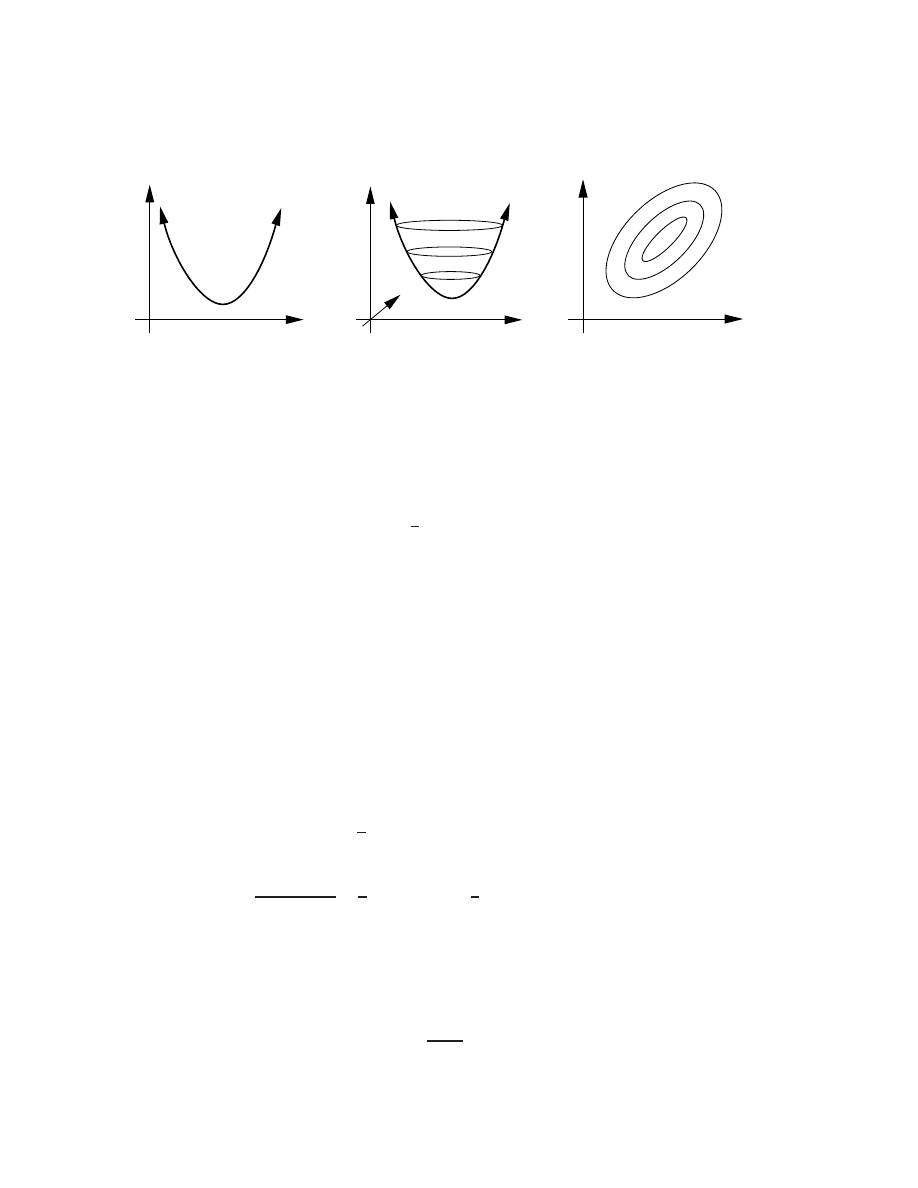
54
CHAPTER
5.
MINIMIZA
TION
J(x)
x
J(x)
x
1
x
2
x
1
x
2
One variable
Two variables (oblique view)
Two variables (top view)
Figure 5.2: Geometry of the minimization problem for quadratic functions. The ellipses in the two
gures on the right indicate isosurfaces of constant
J
.
5.3.1 Steepest descent for quadratic functions
Consider a quadratic function
J
(
x
) of the form
J
(
x
) = 12
x
T
A
x
;
b
T
x
where
A
is positive denite. The geometry of this problem is illustrated in Figure 5.2.
We will begin at some initial guess
x
(0)
and move at each step of the iteration
k
in a direction
downhill
r
(
k
)
such that
x
(
k
+1)
=
x
(
k
)
+
(
k
)
r
(
k
)
where
(
k
)
is a parameter for the descent which will be determined. In this manner, we proceed
iteratively towards the minimum of
J
(
x
). Noting the derivation of
rJ
in
x
5.1.1, dene
r
(
k
)
as the
direction of steepest descent such that
r
(
k
)
=
;r
J
(
x
(
k
)
) =
;
(
A
x
(
k
)
;
b
)
:
Now that we have gured out what direction we will update
x
(
k
)
, we need to gure out the parameter
of descent
(
k
)
, which governs the distance we will update
x
(
k
)
in this direction. This may be found
by minimizing
J
(
x
(
k
)
+
(
k
)
r
(
k
)
) with respect to
(
k
)
. Dropping the superscript ()
(
k
)
for the time
being for notational clarity, note rst that
J
(
x
+
r
) = 12(
x
+
r
)
T
A
(
x
+
r
)
;
b
T
(
x
+
r
)
and thus
@
J
(
x
+
r
)
@
= 12
r
T
A
(
x
+
r
) + 12(
x
+
r
)
T
A
r
;
b
T
r
=
r
T
A
r
+
r
T
A
x
;
r
T
b
=
r
T
A
r
+
r
T
(
A
x
;
b
)
=
r
T
A
r
;
r
T
r
:
Setting
@
J
(
x
+
r
)
=@
= 0 yields
=
r
T
r
r
T
A
r
:

5.3.
GRADIENT-BASED
APPR
O
A
CHES
F
OR
MINIMIZA
TION
OF
MUL
TIV
ARIABLE
FUNCTIONS
55
Thus, from the value of
x
(
k
)
at each iteration, we can determine explicitly both the direction of
descent
r
(
k
)
and the parameter
(
k
)
which minimizes
J
.
Matlab implementation
% sd_quad.m
% Minimize a quadratic function J(x) = (1/2) x^T A x - b^T x
% using the steepest descent method
clear res_save x_save epsilon=1e-6 x=zeros(size(b))
for iter=1:itmax
r=b-A*x
% determine gradient
res=r'*r
% compute residual
res_save(iter)=res x_save(:,iter)=x
% save some stuff
if (res<epsilon | iter==itmax), break end
% exit yet?
alpha=res/(r'*A*r)
% compute alpha
x=x+alpha*r
% update x
end
% end sd_quad.m
Operation count
The operation count for each iteration of the steepest descent algorithm may be determined by
inspection of the above code, and is calculated in the following table.
Operation
ops
To compute
A
x
;
b
:
O
(2
n
2
)
To compute
r
T
r
:
O
(2
n
)
To compute
r
T
A
r
:
O
(2
n
2
)
To compute
x
+
r
:
O
(2
n
)
TOTAL:
O
(4
n
2
)
A cheaper technique for computing such an algorithm is discussed at the end of the next section.
5.3.2 Conjugate gradient for quadratic functions
As discussed earlier, and shown in Figure 5.3, proceeding in the direction of steepest descent at each
iteration is not necessarily the most ecient strategy. By so doing, the path of the algorithm can be
very jagged. Due to the successive line minimizations and the lack of momentum from one iteration
to the next, the steepest descent algorithm must tack back and forth 90
at each turn. We now
show that, by slight modication of the steepest descent algorithm, we arrive at the vastly improved
conjugate gradient algorithm. This improved algorithm retains the correct amount of momentum
from one iteration to the next to successfully negotiate functions
J
(
x
) with narrow valleys.
Note that in \easy" cases for which the condition number is approximately unity, the level
surfaces of
J
are approximately circular, and convergence with either the steepest descent or the
conjugate gradient algorithm will be quite rapid. In poorly conditioned problems, the level surfaces
become highly elongated ellipses, and the zig-zag behavior is amplied.
Instead of minimizing in a single search direction at each iteration, as we did for the method of
steepest descent, now consider searching simultaneously in
m
directions, which we will denote
p
(0)
,
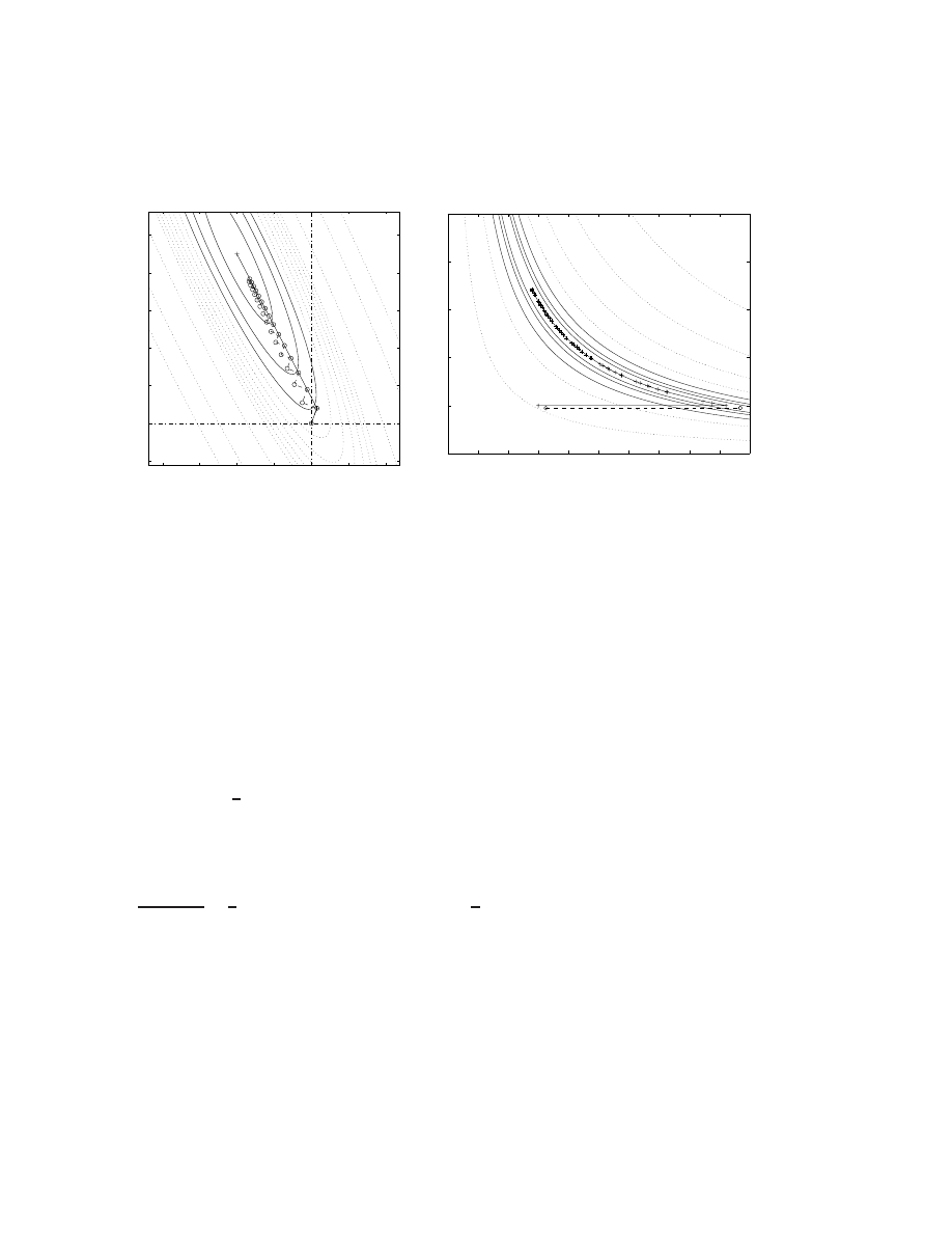
56
CHAPTER
5.
MINIMIZA
TION
−8
−6
−4
−2
0
2
4
−2
0
2
4
6
8
10
0
0.2
0.4
0.6
0.8
1
1.2
1.4
1.6
1.8
2
x 10
−8
0
1
2
3
4
5
x 10
−5
a) Quadratic
J
3
(
1
2
).
b) Non-quadratic
J
4
(
1
2
).
Minimum point
Minimum point
Starting
point
Starting
point
Figure 5.3: Convergence of: (
) simple gradient, and (
+
) the conjugate gradient algorithms when
applied to nd minima of two test functions of two scalar control variables
x
1
and
x
2
(horizontal and
vertical axes). Contours illustrate the level surfaces of the test functions contours corresponding to
the smallest isovalues are solid, those corresponding to higher isovalues are dotted.
p
(1)
,
:::
p
(
m
;
1)
. Take
x
(
m
)
=
x
(0)
+
m
;
1
X
j
=0
(
j
)
p
(
j
)
and note that
J
(
x
(
m
)
) = 12
x
(0)
+
m
;
1
X
j
=0
(
j
)
p
(
j
)
T
A
x
(0)
+
m
;
1
X
j
=0
(
j
)
p
(
j
)
;
b
T
x
(0)
+
m
;
1
X
j
=0
(
j
)
p
(
j
)
:
Taking the derivative of this expression with respect to
(
k
)
,
@
J
(
x
(
m
)
)
@
(
k
)
= 12
p
(
k
)
T
A
x
(0)
+
m
;
1
X
j
=0
(
j
)
p
(
j
)
+ 12
x
(0)
+
m
;
1
X
j
=0
(
j
)
p
(
j
)
T
A
p
(
k
)
;
b
T
p
(
k
)
=
(
k
)
p
(
k
)
T
A
p
(
k
)
+
p
(
k
)
T
A
x
(0)
;
p
(
k
)
T
b
+
m
;
1
X
j
=0
j
6=k
(
j
)
p
(
k
)
T
A
p
(
j
)
:
We seek a technique to select all the
p
(
j
)
in such a way that they are orthogonal through
A
, or
conjugate, such that
p
(
k
)
T
A
p
(
j
)
= 0 for
j
6
=
k:

5.3.
GRADIENT-BASED
APPR
O
A
CHES
F
OR
MINIMIZA
TION
OF
MUL
TIV
ARIABLE
FUNCTIONS
57
IF
we can nd such a sequence of
p
(
j
)
, then we obtain
@
J
(
x
m
)
@
(
k
)
=
(
k
)
p
(
k
)
T
A
p
(
k
)
+
p
(
k
)
T
A
x
(0)
;
b
=
(
k
)
p
(
k
)
T
A
p
(
k
)
;
p
(
k
)
T
r
(0)
and thus setting
@
J
=@
(
k
)
= 0 results in
(
k
)
=
p
(
k
)
T
r
(0)
p
(
k
)
T
A
p
(
k
)
:
The remarkable thing about this result is that it is independent of
p
(
j
)
for
j
6
=
k
! Thus, so long
as we can nd a way to construct a sequence of
p
(
k
)
which are all conjugate, then each of these
minimizations may be done separately.
The conjugate gradient technique is simply an ecient technique to construct a sequence of
p
(
k
)
which are conjugate. It entails just redening the descent direction
p
(
k
)
at each iteration after the
rst to be a linear combination of the direction of steepest descent,
r
(
k
)
, and the descent direction
at the previous iteration,
p
(
k
;
1)
, such that
p
(
k
)
=
r
(
k
)
+
p
(
k
;
1)
and
x
(
k
+1)
=
x
(
k
)
+
p
(
k
)
where
and
are given by
=
r
(
k
)
T
r
(
k
)
r
(
k
;
1)
T
r
(
k
;
1)
=
r
(
k
)
T
r
(
k
)
p
(
k
)
T
A
p
(
k
)
:
Verication that this choice of
results in conjugate directions and that this choice of
is equivalent
to the one mentioned previously (minimizing
J
in the direction
p
(
k
)
from the point
x
(
k
)
) involves
a straightforward (but lengthy) proof by induction. The interested reader may nd this proof in
Golub and van Loan (1989).
Matlab implementation
% cg_quad.m
% Minimize a quadratic function J=(1/2) x^T A x - b^T x
% using the conjugate gradient method
clear res_save x_save epsilon=1e-6 x=zeros(size(b))
for iter=1:itmax
r=b-A*x
% determine gradient
res=r'*r
% compute residual
res_save(iter)=res x_save(:,iter)=x
% save some stuff
if (res<epsilon | iter==itmax), break end
% exit yet?
if (iter==1)
% compute update direction
p = r
% set up a S.D. step
else
beta = res / res_save(iter-1)
% compute momentum term
p = r + beta * p
% set up a C.G. step
end

58
CHAPTER
5.
MINIMIZA
TION
alpha=res/(p'*A*p)
% compute alpha
x=x+alpha*p
% update x
end
% end cg_quad.m
As seen by comparison of the
cg quad.m
to
sd quad.m
, implementation of the conjugate gradient
algorithm involves only a slight modication of the steepest descent algorithm. The operation count
is virtually the same (
cg quad.m
requires 2
n
more ops per iteration), and the storage requirements
are slightly increased (
cg quad.m
denes an extra
n
-dimensional vector
p
).
Matlab implementation - cheaper version
A cheaper version of
cg quad
may be written by leveraging the fact that an iterative procedure may
developed for the computation of
r
by combining the following two equations:
x
(
k
)
=
x
(
k
;
1)
+
(
k
;
1)
p
(
k
;
1)
r
(
k
)
=
b
;
A
x
(
k
)
:
Putting these two equations together leads to an update equation for
r
at each iteration:
r
(
k
)
=
b
;
A
(
x
(
k
;
1)
+
(
k
;
1)
p
(
k
;
1)
) =
r
(
k
;
1)
;
(
k
;
1)
A
p
(
k
;
1)
:
The nice thing about this update equation for
r
, versus the direct calculation of
r
, is that this update
equation depends on the matrix/vector product
A
p
(
k
;
1)
, which needs to be computed anyway during
the computation of
. Thus, for quadratic functions, an implementation which costs only
O
(2
n
2
)
per iteration is possible, as given by the following code:
% cg_cheap_quad.m
% Minimize a quadratic function J=(1/2) x^T A x - b^T x
% using the conjugate gradient method
clear res_save x_save epsilon=1e-6 x=zeros(size(b))
for iter=1:itmax
if (iter==1)
r=b-A*x
% determine r directly
else
r=r-alpha*d
% determine r by the iterative formula.
end
res=r'*r
% compute residual
res_save(iter)=res x_save(:,iter)=x
% save some stuff
if (res<epsilon | iter==itmax), break end
% exit yet?
if (iter==1)
% compute update direction
p = r
% set up a S.D. step
else
beta = res / res_save(iter-1)
% compute momentum term
p = r + beta * p
% set up a C.G. step
end
d=A*p
% perform the (expensive) matrix/vector product
alpha=res/(p'*d)
% compute alpha
x=x+alpha*p
% update x

5.3.
GRADIENT-BASED
APPR
O
A
CHES
F
OR
MINIMIZA
TION
OF
MUL
TIV
ARIABLE
FUNCTIONS
59
end
% end cg_cheap_quad.m
A test code named
test sd cg.m
, which is available at the class web site, may be used to check to
make sure these steepest descent and conjugate gradient algorithms work as advertized. These codes
also produce some nice plots to get a graphical interpretation of the operation of the algorithms.
5.3.3 Preconditioned conjugate gradient
Assuming exact arithmetic, the conjugate gradient algorithm converges in exactly
N
iterations for
an
N
-dimensional quadratic minimization problem. For large
N
, however, we often can not aord
to perform
N
iterations. We often seek to perform approximate minimization of an
N
-diminsional
problem with a total number of iterations
m
N
. Unfortunately, convergence of the conjugate
gradient algorithm to the minimum of
J
, though monotonic, is often highly nonuniform, so large
reductions in
J
might not occur until iterations well after the iteration
m
at which we would like
to truncate the iteration sequence.
The uniformity of the convergence is governed by the condition number
c
of the matrix
A
,
which (for symmetric positive-denite
A
) is just equal to the ratio of its maximum and minimum
eigenvalues,
max
=
min
. For small
c
, convergence of the conjugate gradient algorithm is quite rapid
even for high-dimensional problems with
N
1.
We therefore seek to solve a better conditioned but equivalent problem ~
A
~
x
= ~
b
which, once
solved, will allow us to easily extract the solution of the original problem
A
x
=
b
for a poorly-
conditioned symmetric positive denite
A
. To accomplish this, premultiply
A
x
=
b
by
P
;
1
for
some symmetric preconditioning matrix
P
:
P
;
1
A
x
=
P
;
1
b
)
(
P
;
1
AP
;
1
)
|
{z
}
~
A
P
x
|{z}
~
x
=
P
;
1
b
|
{z
}
~
b
Note that the matrix
P
;
1
AP
;
1
is symmetric positive denite. We will defer discussion of the
construction of an appropriate
P
to the end of the section suce it to say for the moment that,
if
P
2
is somehow \close" to
A
, then the problem ~
A
~
x
= ~
b
is a well conditioned problem (because
~
A
=
P
;
1
AP
;
1
I
) and can be solved rapidly (with a small number of iterations) using the
conjugate gradient approach.
The computation of ~
A
might be prohibitively expensive and destroy any sparsity structure of
A
.
We now show that it is not actually necessary to compute ~
A
and ~
b
in order to solve the original
problem
A
x
=
b
in a well conditioned manner. To begin, we write the conjugate gradient algorithm
for the well conditioned problem ~
A
~
x
= ~
b
. For simplicity, we use a short-hand (\pseudo-code")
notation:

60
CHAPTER
5.
MINIMIZA
TION
for
i
= 1 :
m
~
r
(
~
b
;
~
A
~
x
i
= 1
~
r
;
~
d
i >
1
res
old
=
res
res
= ~
r
T
~
r
~
p
(
~
r
i
= 1
~
r
+
~
p
where
=
res=res
old
i >
1
=
res=
(~
p
T
~
d
) where ~
d
= ~
A
~
p
~
x
~
x
+
~
p
end
For clarity of notation, we have introduced a tilde over each vector involed in this optimization.
Note that, in converting the poorly-conditioned problem
A
x
=
b
to the well-conditioned problem
~
A
~
x
= ~
b
, we made the following denitions: ~
A
=
P
;
1
AP
;
1
, ~
x
=
P
x
, and ~
b
=
P
;
1
b
. Dene now
some new intermediate variables
r
=
P
~
r
,
p
=
P
;
1
~
p
, and
d
=
P
~
d
. With these denitions, we now
rewrite exactly the above algorithm for solving the well-conditioned problem ~
A
~
x
= ~
b
, but substitute
in the non-tilde variables:
for
i
= 1 :
m
P
;
1
r
(
P
;
1
b
;
(
P
;
1
AP
;
1
)
P
x
i
= 1
P
;
1
r
;
P
;
1
d
i >
1
res
old
=
res
res
= (
P
;
1
r
)
T
(
P
;
1
r
)
P
p
(
P
;
1
r
i
= 1
P
;
1
r
+
P
p
where
=
res=res
old
i >
1
=
res=
!(
P
p
)
T
(
P
;
1
d
)] where
P
;
1
d
= (
P
;
1
AP
;
1
)
P
p
P
x
P
x
+
P
p
end
Now dene
M
=
P
2
and simplify:
for
i
= 1 :
m
r
(
b
;
A
x
i
= 1
r
;
d
i >
1
res
old
=
res
res
=
r
T
s
where
s
=
M
;
1
r
p
(
s
i
= 1
s
+
p
where
=
res=res
old
i >
1
=
res=
!
p
T
d
] where
d
=
A
p
x
x
+
p
end
This is practically identical to the original conjugate gradient algorithm for solving the problem
A
x
=
b
. The new variable
s
=
M
;
1
r
may be found by solution of the system
M
s
=
r
. Thus,

5.3.
GRADIENT-BASED
APPR
O
A
CHES
F
OR
MINIMIZA
TION
OF
MUL
TIV
ARIABLE
FUNCTIONS
61
when implementing this method, we seek an
M
for which we can solve this system quickly (e.g., an
M
which is the product of sparse triangular matrices). Recall that if
M
=
P
2
is somehow \close"
to
A
, the problem here (which is actually the solution of ~
A
~
x
= ~
b
via standard conjugate gradient)
is well conditioned and converges in a small number of iterations. There are a variety of heuristic
techniques to construct an appropriate
M
. One of the most popular is
incomplete Cholesky
factorization
, which constructs a triangular
H
with
HH
T
=
M
A
with the following strategy:
H
=
A
for
k
= 1 :
n
H
(
kk
) =
p
H
(
kk
)
for
i
=
k
+ 1 :
n
if
H
(
ik
)
6
= 0 then
H
(
ik
) =
H
(
ik
)
=H
(
kk
)
end
for
j
=
k
+ 1 :
n
for
i
=
j
:
n
if
H
(
ij
)
6
= 0 then
H
(
ij
) =
H
(
ij
)
;
H
(
ik
)
H
(
jk
)
end
end
end
Once
H
is obtained with this appraoch such that
HH
T
=
M
, solving the system
M
s
=
r
for
s
is similar to solving Gaussian elimination by leveraging an LU decomposition: one rst solves the
triangular system
H
f
=
r
for the intermediate variable
f
, then solves the triangular system
H
T
s
=
f
for the desired quantity
s
.
Note that the triangular factors
H
and
H
T
are zero everywhere
A
is zero. Thus, if
A
is sparse,
the above algorithm can be rewritten in a manner that leverages the sparsity structure of
H
(akin
to the backsubstitution in the Thomas algorithm). Though it is sometimes takes a bit of eort to
write an algorithm that eciently leverages such sparsity structure, as it usually must be done on
a case-by-case basis, the benets of preconditioning are often quite signicant and well worth the
coding eort which it necessitates.
Motivation and further discussion of incomplete Cholesky factorization, as well as other precon-
ditioning techniques, is deferred to Golub and van Loan (1989).
5.3.4 Extension non-quadratic functions
At each iteration of the conjugate gradient method, there are ve things to be done:
1. Determine the (negative of) the gradient direction,
r
=
;r
J
,
2. compute the residual
r
T
r
,
3. determine the necessary momentum
and the corresponding update direction
p
r
+
p
,
4. determine the (scalar) parameter of descent
which minimizes
J
(
x
+
p
), and
5. update
x
x
+
p
.

62
In the homework, you will extend the codes developed here for quadratic problems to nonquadratic
problems, creating two new routines
sd nq.m
and
cg nq.m
. Essentially, the algorithm is the same,
but
J
(
x
) now lacks the special quadratic structure we assumed in the previous sections. Generalizing
the results of the previous sections to nonquadratic problems entails only a few modications:
1'. Replace the line which determines the gradient direction with a call to a function, which we
will call
compute grad.m
, which calculates the gradient
r
J
of the nonquadratic function
J
.
3'. As the function is not quadratic, but the momentum term in the conjugate gradient algorithm
is computed using a local quadratic approximation of
J
, the momentum sometimes builds up
in the wrong direction. Thus, the momentum should be reset to zero (i.e., take
= 0) every
R
iterations in
cg nq.m
(
R
= 20 is often a good choice).
4'. Replace the direct computation of
with a call to an (appropriately modied) version of
Brent's method to determine
based on a series of function evaluations.
Finally, when working with nonquadratic functions, it is often adventageous to compute the
momentum term
according to the formula
= (
r
(
k
)
;
r
(
k
;
1)
)
T
r
(
k
)
(
r
(
k
;
1)
)
T
r
(
k
;
1)
The \correction" term (
r
(
k
;
1)
)
T
r
(
k
)
is zero using the conjugate gradient approach when the function
J
is quadratic. When the function
J
is not quadratic, this additional term often serves to nudge
the descent direction towards that of a steepest descent step in regions of the function which are
highly nonquadratic. This approach is referred to as the
Polak-Ribiere
variant of the conjugate
gradient method for nonquadratic functions.

Chapter
6
Dierentiation
6.1 Derivation of nite dierence formulae
In the simulation of physical systems, one often needs to compute the derivative of a function
f
(
x
)
which is known only at a discrete set of grid points
x
0
x
1
::: x
N
. Eective formulae for computing
such approximations, known as nite dierence formulae, may be derived by combination of one or
more Taylor series expansions. For example, dening
f
j
=
f
(
x
j
), the Taylor series expansion for
f
at point
x
j
+1
in terms of
f
and its derivatives at the point
x
j
is given by
f
j
+1
=
f
j
+ (
x
j
+1
;
x
j
)
f
0
j
+ (
x
j
+1
;
x
j
)
2
2!
f
00
j
+ (
x
j
+1
;
x
j
)
3
3!
f
000
j
+
:::
Dening
h
j
=
x
j
+1
;
x
j
, rearrangement of the above equation leads to
f
0
j
=
f
j
+1
;
f
j
h
j
;
h
j
2
f
00
j
+
:::
In these notes, we will indicate a uniform mesh by denoting its (constant) grid spacing as
h
(without
a subscript), and we will denote a nonuniform (\stretched") mesh by denoting the grid spacing as
h
j
(with a subscript). We will assume the mesh is uniform unless indicated otherwise. For a uniform
mesh, we may write the above equation as
f
0
j
=
f
j
+1
;
f
j
h
+
O
(
h
)
where
O
(
h
) denotes the contribution from all terms which have a power of
h
which is greater then
or equal to one. Neglecting these \higher-order terms" for suciently small
h
, we can approximate
the derivative as
f
x
j
=
f
j
+1
;
f
j
h
which is referred to as the rst-order forward dierence formula for the rst derivative. The neglected
term with the highest power of
h
(in this case,
;
hf
0
0
j
=
2) is referred to as the leading-order error. The
exponent of
h
in the leading-order error is the order of accuracy of the method. For a suciently
ne initial grid, if we rene the grid spacing further by a factor of two, the truncation error of this
method is also reduced by approximately a factor of 2, indicating a \rst-order" behavior.
63

64
CHAPTER
6.
DIFFERENTIA
TION
Similarly, by expanding
f
j
;
1
about the point
x
j
and rearranging, we obtain
f
x
j
=
f
j
;
f
j
;
1
h
which is referred to as the rst-order backward dierence formula for the rst derivative. Higher-
order (more accurate) schemes can be derived by combining Taylor series of the function
f
at various
points near the point
x
j
. For example, the widely used second-order central dierence formula for
the rst derivative can be obtained by subtraction of the two Taylor series expansions
f
j
+1
=
f
j
+
hf
0
j
+
h
2
2
f
0
0
j
+
h
3
6
f
000
j
+
:::
f
j
;
1
=
f
j
;
hf
0
j
+
h
2
2
f
0
0
j
;
h
3
6
f
000
j
+
:::
leading to
f
j
+1
;
f
j
;
1
= 2
hf
0
j
+
h
3
3
f
000
j
+
:::
and thus
f
0
j
=
f
j
+1
;
f
j
;
1
2
h
;
h
2
6
f
000
j
+
:::
)
f
x
j
=
f
j
+1
;
f
j
;
1
2
h
:
Similar formulae can be derived for second-order derivatives (and higher). For example, by adding
the above Taylor series expansions instead of subtracting them, we obtain the second-order central
dierence formula for second derivative given by
f
0
0
j
=
f
j
+1
;
2
f
j
+
f
j
;
1
h
2
;
h
2
24
f
IV
j
+
:::
)
2
f
x
2
j
=
f
j
+1
;
2
f
j
+
f
j
;
1
h
2
:
In general, we can obtain higher accuracy if we include more points. By approximate linear com-
bination of four dierent Taylor Series expansions, a fourth-order central dierence formula for the
rst derivative may be found, which takes the form
f
x
j
=
f
j
;
2
;
8
f
j
;
1
+ 8
f
j
+1
;
f
j
+2
12
h
:
The main diculty with higher order formulae occurs near boundaries of the domain. They require
the functional values at points outside the domain which are not available. Near boundaries one
usually resorts to lower order formulae.
6.2 Taylor Tables
There is a general technique for constructing nite dierence formulae using a tool known as a
Taylor Table. This technique is best illustrated by example. Suppose we want to construct the most
accurate nite dierence scheme for the rst derivative that involves the function values
f
j
,
f
j
+1
,
and
f
j
+2
. Given this restriction on the information used, we seek the highest order of accuracy that
can be achieved. That is, if we take
f
0
j
;
2
X
=0
a
f
j
+
=
(6.1)

6.3.
P
AD
E
APPR
O
XIMA
TIONS
65
where the
a
are the coecients of the nite dierence formula sought, then we desire to select
the
a
such that the error
is as large a power of
h
as possible (and thus will vanish rapidly upon
renement of the grid). It is convenient to organize the Taylor series of the terms in the above
formula using a \Taylor Table" of the form
f
j
f
0
j
f
0
0
j
f
0
0 0
j
f
0
j
;
a
0
f
j
;
a
1
f
j
+1
;
a
2
f
j
+2
0
1
0
0
;
a
0
0
0
0
;
a
1
;
a
1
h
;
a
1
h
2
2
;
a
1
h
3
6
;
a
2
;
a
2
(2
h
)
;
a
2 (2
h
)
2
2
;
a
2 (2
h
)
3
6
The leftmost column of this table contains all of the terms on the left-hand side of (6.1). The
elements to the right, when multiplied by the corresponding terms at the top of each column and
summed, yield the Taylor series expansion of each of the terms to the left. Summing up all of these
terms, we get the error
expanded in terms of powers of the grid spacing
h
. By proper choice of
the available degrees of freedom
f
a
0
a
1
a
2
g
, we can set several of the coecients of this polynomial
equal to zero, thereby making
as high a power of
h
as possible. For small
h
, this is a good way
of making this error small. In the present case, we have three free coecients, and can set the
coecients of the rst three terms to zero:
;
a
0
;
a
1
;
a
2
= 0
1
;
a
1
h
;
a
2
(2
h
) = 0
;
a
1
h
2
2
;
a
2
(2
h
)
2
2 = 0
9
>
>
=
>
>
)
0
@
;
1
;
1
;
1
0
;
1
;
2
0
;
1
=
2
;
2
1
A
0
@
a
0
h
a
1
h
a
2
h
1
A
=
0
@
0
;
1
0
1
A
)
0
@
a
0
a
1
a
2
1
A
=
0
@
;
3
=
(2
h
)
2
=h
;
1
=
(2
h
)
1
A
This simple linear system may be solved either by hand or with Matlab. The resulting second-order
forward dierence formula for the rst derivative is
f
x
j
=
;
3
f
j
+ 4
f
j
+1
;
f
j
+2
2
h
and the leading-order error, which can be determined by multiplying the rst non-zero column sum
by the term at the top of the corresponding column, is
;
a
1
h
3
6
;
a
2
(2
h
)
3
6
f
0
0 0
j
=
h
2
3
f
0
00
j
revealing that this scheme is second-order accurate.
6.3 Pade Approximations
By including both nearby function evaluations and nearby gradient approximations on the left hand
side of an expression like (6.1), we can derive a banded system of equations which can easily be
solved to determine a numerical approximation of the
f
0
j
. This approach is referred to as
Pade
approximation
. Again illustrating by example, consider the equation
b
;
1
f
0
j
;
1
+
f
0
j
+
b
1
f
0
j
+1
;
1
X
k
=
;
1
a
f
j
+
=
:
(6.2)
66
CHAPTER
6.
DIFFERENTIA
TION
Leveraging the Taylor series expansions
f
j
+1
=
f
j
+
hf
0
j
+
h
2
2
f
00
j
+
h
3
6
f
000
j
+
h
4
24
f
(
iv
)
j
+
h
5
120
f
(
v
)
j
+
:::
f
0
j
+1
=
f
0
j
+
hf
00
j
+
h
2
2
f
000
j
+
h
3
6
f
(
iv
)
j
+
h
4
24
f
(
v
)
j
+
:::
the corresponding Taylor table is
f
j
f
0
j
f
00
j
f
000
j
f
(
iv
)
j
f
(
v
)
j
b
;
1
f
0
j
;
1
f
0
j
b
1
f
0
j
+1
;
a
;
1
f
j
;
1
;
a
0
f
j
;
a
1
f
j
+1
0
b
;
1
b
;
1
(
;
h
)
b
;
1 (
;
h
)
2
2
b
;
1 (
;
h
)
3
6
b
;
1 (
;
h
)
4
24
0
1
0
0
0
0
0
b
1
b
1
h
b
1
h
2
2
b
1
h
3
6
b
1
h
4
24
;
a
;
1
;
a
;
1
(
;
h
)
;
a
;
1 (
;
h
)
2
2
;
a
;
1 (
;
h
)
3
6
;
a
;
1 (
;
h
)
4
24
;
a
;
1 (
;
h
)
5
120
;
a
0
0
0
0
0
0
;
a
1
;
a
1
h
;
a
1
h
2
2
;
a
1
h
3
6
;
a
1
h
4
24
;
a
1
h
5
120
We again use the available degrees of freedom
f
b
;
1
b
1
a
;
1
a
0
a
1
g
to obtain the highest possible
accuracy in (6.2). Setting the sums of the rst ve columns equal to zero leads to the linear system
0
B
B
B
B
@
0
0
;
1
;
1
;
1
1
1
h
0
;
h
;
h
h
;
h
2
=
2 0
;
h
2
=
2
h
2
=
2
h
2
=
2
h
3
=
6
0
;
h
3
=
6
;
h
3
=
6
h
3
=
6
;
h
4
=
24 0
;
h
4
=
24
1
C
C
C
C
A
0
B
B
B
B
@
b
;
1
b
1
a
;
1
a
0
a
1
1
C
C
C
C
A
=
0
B
B
B
B
@
0
;
1
0
0
0
1
C
C
C
C
A
which is equivalent to
0
B
B
B
B
@
0
0
;
1
;
1
;
1
1
1
1
0
;
1
;
1
1
;
1
=
2 0
;
1
=
2
1
=
2 1
=
2 1
=
6
0
;
1
=
6
;
1
=
6 1
=
6
;
1
=
24 0
;
1
=
24
1
C
C
C
C
A
0
B
B
B
B
@
b
;
1
b
1
a
;
1
h
a
0
h
a
1
h
1
C
C
C
C
A
=
0
B
B
B
B
@
0
;
1
0
0
0
1
C
C
C
C
A
)
0
B
B
B
B
@
b
;
1
b
1
a
;
1
a
0
a
1
1
C
C
C
C
A
=
0
B
B
B
B
@
1
=
4
1
=
4
3
=
(4
h
)
0
;
3
=
(4
h
)
1
C
C
C
C
A
Thus, the system to be solved to determine the numerical approximation of the derivatives at each
grid point has a typical row given by
1
4
f
x
j
+1
+
f
x
j
+ 14
f
x
j
;
1
= 34
h
f
j
+1
;
f
j
;
1
and has a leading-order error of
h
4
f
(
v
)
j
=
30, and thus is fourth-order accurate. Writing out this
equation for all values of
j
on the interior leads to the tridiagonal, diagonally-dominant system
0
B
B
B
B
B
B
@
... ... ...
1
4
1
1
4
... ... ...
1
C
C
C
C
C
C
A
0
B
B
B
B
B
B
B
B
B
B
@
...
f
x
j
;
1
f
x
j
f
x
j
+1
...
1
C
C
C
C
C
C
C
C
C
C
A
=
0
B
B
B
B
B
B
B
B
B
@
...
...
3
4
h
f
j
+1
;
f
j
;
1
...
...
1
C
C
C
C
C
C
C
C
C
A
:

6.4.
MODIFIED
W
A
VENUMBER
ANAL
YSIS
67
At the endpoints, a dierent treatment is needed a central expression (Pade or otherwise) cannot
be used at
x
0
because
x
;
1
is outside of our available grid of data. One commonly settles on a
lower-order forward (backward) expression at the left (right) boundary in order to close this set of
equations in a nonsingular manner. This system can then be solved eciently for the numerical
approximation of the derivative at all of the gridpoints using the Thomas algorithm.
6.4 Modied wavenumber analysis
The order of accuracy is usually the primary indicator of the accuracy of nite-dierence formulae
it tells us how mesh renement improves the accuracy. For example, for a suciently ne grid, mesh
renement by a factor of two improves the accuracy of a second-order nite-dierence scheme by a
factor of four, and improves the accuracy of a fourth-order scheme by a factor of sixteen. Another
method for quantifying the accuracy of a nite dierence formula that yields further information is
called the
modied wavenumber
approach. To illustrate this approach, consider the harmonic
function given by
f
(
x
) =
e
ik x
(6.3)
(Alternatively, we can also do this derivation with sines and cosines, but complex exponentials tend
to make the algebra easier.) The exact derivative of this function is
f
0
=
ik e
ik x
=
ik f
(6.4)
We now ask how accurately the second order central nite-dierence scheme, for example, computes
the derivative of
f
. Let us discretize the
x
axis with a uniform mesh,
x
j
=
h
j
where
j
= 0
1
2
::: N
and
h
=
L
N :
The nite-dierence approximation for the derivative which we consider here is
f
x
j
=
f
j
+1
;
f
j
;
1
2
h
Substituting for
f
j
=
e
ik x
j
, noting that
x
j
+1
=
x
j
+
h
and
x
j
;
1
=
x
j
;
h
, we obtain
f
x
j
=
e
ik
(
x
j
+
h
)
;
e
ik
(
x
j
;
h
)
2
h
=
e
ik h
;
e
;
ik h
2
h
f
j
=
i
sin(
hk
)
h f
j
,
ik
0
f
j
(6.5)
where
k
0
,
sin
hk
h
)
hk
0
= sin(
hk
)
By analogy with (6.4),
k
0
is called the modied wave number for this second-order nite dierence
scheme. In an analogous manner, one can derive modied wave numbers for any nite dierence
formula. A measure of accuracy of the nite-dierence scheme is provided by comparing the modied
wavenumber
k
0
, which appears in the numerical approximation of the derivative (6.5), with the
actual wavenumber
k
, which appears in the exact expression for the derivative (6.4). For small
wavenumbers, the numerical approximation of the derivative on our discrete grid is usually pretty
good (
k
0
k
), but for large wavenumbers, the numerical approximation is degraded. As
k
!
=h
,
the numerical approximation of the derivative is completely o.

68
As another example, consider the modied wavenumber for the fourth-order expression of rst
derivative given by
f
x
j
=
f
j
;
2
;
8
f
j
;
1
+ 8
f
j
+1
;
f
j
+2
12
h
= 23
h
(
f
j
+1
;
f
j
;
1
)
;
1
12
h
(
f
j
+2
;
f
j
;
2
)
:
Inserting (6.3) and manipulating as before, we obtain:
f
x
j
= 23
h
(
e
ik h
;
e
;
ik h
)
f
j
;
1
12(
e
ik
2
h
;
e
;
ik
2
h
)
f
j
=
i
h
4
3
h
sin(
hk
)
;
1
6
h
sin(2
hk
)
i
f
j
,
ik
0
f
j
)
hk
0
= 43 sin(
hk
)
;
1
6 sin(2
hk
)
Consider now our fourth-order Pade approximation:
1
4
f
x
j
+1
+
f
x
j
+ 14
f
x
j
;
1
= 34
h
f
j
+1
;
f
j
;
1
Approximating the modied wavenumber at points
x
j
+1
and
x
j
;
1
with their corresponding numerical
approximations
f
x
j
+1
=
ik
0
e
ik x
j
+1
=
ik
0
e
ik h
f
j
and
f
x
j
;
1
=
ik
0
e
ik x
j
;1
=
ik
0
e
;
ik h
f
j
and inserting (6.3) and manipulating as before, we obtain:
ik
0
1
4
e
ik h
+ 1 + 14
e
;
ik h
f
j
= 34
h
(
e
ik h
;
e
;
ik h
)
f
j
ik
0
1 + 12 cos(
hk
)
f
j
=
i
3
2
h
sin(
hk
)
f
j
)
hk
0
=
3
2
sin(
hk
)
1 +
1
2
cos(
hk
)
6.5 Alternative derivation of dierentiation formulae
Consider now the Lagrange interpolation of the three points
f
x
i
;
1
f
i
;
1
g
,
f
x
i
f
i
g
, and
f
x
i
+1
f
i
+1
g
,
given by:
f
(
x
) = (
x
;
x
i
)(
x
;
x
i
+1
)
(
x
i
;
1
;
x
i
)(
x
i
;
1
;
x
i
+1
)
f
i
;
1
+ (
x
;
x
i
;
1
)(
x
;
x
i
+1
)
(
x
i
;
x
i
;
1
)(
x
i
;
x
i
+1
)
f
i
+ (
x
;
x
i
;
1
)(
x
;
x
i
)
(
x
i
+1
;
x
i
;
1
)(
x
i
+1
;
x
i
)
f
i
+1
Dierentiate this expression with respect to
x
and then evaluating at
x
=
x
i
gives
f
0
(
x
i
) = (
;
h
)
(
;
h
)(
;
2
h
)
f
i
;
1
+ 0 + (
h
)
(2
h
)(
h
)
f
i
+1
=
f
i
+1
;
f
i
;
1
2
h
which is the same as what we get with Taylor Table.

Chapter
7
Integration
Dierentiation and integration are two essential tools of calculus which we need to solve engineering
problems. The previous chapter discussed methods to approximate derivatives numerically we now
turn to the problem of numerical integration. In the setting we discuss in the present chapter, in
which we approximate the integral of a given function over a specied domain, this procedure is
usually referred to as
numerical quadrature
.
7.1 Basic quadrature formulae
7.1.1 Techniques based on Lagrange interpolation
Consider the problem of integrating a function
f
on the interval !
ac
] when the function is evaluated
only at a limited number of discrete gridpoints. One approach to approximating the integral of
f
is to integrate the lowest-order polynomial that passes through a specied number of function
evaluations using the formulae of Lagrange interpolation.
For example, if the function is evaluated at the midpoint
b
= (
a
+
c
)
=
2, then (dening
h
=
c
;
a
)
we can integrate a constant approximation of the function over the interval !
ac
], leading to the
midpoint rule
:
Z
c
a
f
(
x
)
dx
Z
c
a
h
f
(
b
)
i
dx
=
hf
(
b
)
,
M
(
f
)
:
(7.1)
If the function is evaluated at the two endpoints
a
and
c
, we can integrate a linear approximation
of the function over the interval !
ac
], leading to the
trapezoidal rule
:
Z
c
a
f
(
x
)
dx
Z
c
a
h
(
x
;
c
)
(
a
;
c
)
f
(
a
) + (
x
;
a
)
(
c
;
a
)
f
(
c
)
i
dx
=
h f
(
a
) +
f
(
c
)
2
,
T
(
f
)
:
(7.2)
If the function is known at all three points
a
,
b
, and
c
, we can integrate a quadratic approximation
of the function over the interval !
ac
], leading to
Simpson's rule
:
Z
c
a
f
(
x
)
dx
Z
c
a
h
(
x
;
b
)(
x
;
c
)
(
a
;
b
)(
a
;
c
)
f
(
a
) + (
x
;
a
)(
x
;
c
)
(
b
;
a
)(
b
;
c
)
f
(
b
) + (
x
;
a
)(
x
;
b
)
(
c
;
a
)(
c
;
b
)
f
(
c
)
i
dx
=
:::
=
h f
(
a
) + 4
f
(
b
) +
f
(
c
)
6
,
S
(
f
)
:
(7.3)
69

70
CHAPTER
7.
INTEGRA
TION
Don't forget that symbolic manipulation packages like Maple (which is included with Matlab) and
Mathematica are well suited for this sort of algebraic manipulation.
7.1.2 Extension to several gridpoints
Recall that Lagrange interpolations are ill-behaved near the endpoints when the number of gridpoints
is large. Thus, it is generally ill-advised to continue the approach of the previous section to function
approximations which are higher order than quadratic. Instead, better results are usually obtained by
applying the formulae of
x
7.1.1 repeatedly over several smaller subintervals. Dening a numerical grid
of points
f
x
0
x
1
::: x
n
g
distributed over the interval !
LR
], the intermediate gridpoints
x
i
;
1
=
2
=
(
x
i
;
1
+
x
i
)
=
2, the grid spacing
h
i
= (
x
i
;
x
i
;
1
), and the function evaluations
f
i
=
f
(
x
i
), the
numerical approximation of the integral of
f
(
x
) over the interval !
LR
] via the midpoint rule takes
the form
Z
R
L
f
(
x
)
dx
n
X
i
=1
h
i
f
i
;
1
=
2
(7.4)
numerical approximation of the integral via the trapezoidal rule takes the form
Z
R
L
f
(
x
)
dx
n
X
i
=1
h
i
f
i
;
1
+
f
i
2
=
h
2
h
f
0
+
f
n
+ 2
n
;
1
X
i
=1
f
i
i
(7.5)
and numerical approximation of the integral via Simpson's rule takes the form
Z
R
L
f
(
x
)
dx
n
X
i
=1
h
i
f
i
;
1
+ 4
f
i
;
1
2
+
f
i
6
=
h
6
h
f
0
+
f
n
+ 4
n
X
i
=1
f
i
;
1
2
+ 2
n
;
1
X
i
=1
f
i
i
(7.6)
where the rightmost expressions assume a uniform grid in which the grid spacing
h
is constant.
7.2 Error Analysis of Integration Rules
In order to quantify the accuracy of the integration rules we have proposed so far, we may again turn
to Taylor series analysis. For example, replacing
f
(
x
) with its Taylor series approximation about
b
and integrating, we obtain
Z
c
a
f
(
x
)
dx
=
Z
c
a
h
f
(
b
) + (
x
;
b
)
f
0
(
b
) + 12 (
x
;
b
)
2
f
0
0
(
b
) + 13 (
x
;
b
)
3
f
0
0 0
(
b
) +
:::
i
dx
=
hf
(
b
) + 12 (
x
;
b
)
2
c
a
f
0
(
b
) + 16 (
x
;
b
)
3
c
a
f
0
0
(
b
) +
:::
=
hf
(
b
) +
h
3
24
f
00
(
b
) +
h
5
1920
f
(
iv
)
(
b
) +
:::
(7.7)
Thus, if the integral is approximated by the midpoint rule (7.1), the leading-order error is propor-
tional to
h
3
, and the approximation of the integral over this single interval is third-order accurate.
Note also that if all even derivatives of
f
happen to be zero (for example, if
f
(
x
) is linear in
x
), the
midpoint rule integrates the function exactly.
The question of the accuracy of a particular integration rule over a single interval is often not
of much interest, however. A more relevant measure is the rate of convergence of the integration

7.3.
R
OMBER
G
INTEGRA
TION
71
rule when applied over several gridpoints on a given interval !
LR
] as the numerical grid is rened.
For example, consider the formula (7.4) on
n
subintervals (
n
+ 1 gridpoints). As
h
/
1
=n
(the
width of each subinterval is inversely proportional to the number of subintervals), the error over
the entire interval !
LR
] of the numerical integration will be proportional to
nh
3
=
h
2
. Thus, for
approximations of the integral on a given interval !
LR
] as the computational grid is rened, the
midpoint rule is second-order accurate
.
Consider now the Taylor series approximations of
f
(
a
) and
f
(
c
) about
b
:
f
(
a
) =
f
(
b
) +
;
h
2
f
0
(
b
) + 12
;
h
2
2
f
00
(
b
) + 16
;
h
2
3
f
000
(
b
) +
:::
f
(
c
) =
f
(
b
) +
h
2
f
0
(
b
) + 12
h
2
2
f
0
0
(
b
) + 16
h
2
3
f
000
(
b
) +
:::
Combining these expressions gives
f
(
a
) +
f
(
c
)
2
=
f
(
b
) + 18
h
2
f
0
0
(
b
) + 1
384
f
(
iv
)
(
b
) +
:::
Solve for
f
(
b
) and substituting into (7.7) yields
Z
c
a
f
(
x
)
dx
=
h f
(
a
) +
f
(
c
)
2
;
h
3
12
f
00
(
b
)
;
h
5
480
f
(
iv
)
(
b
) +
:::
(7.8)
As with the midpoint rule, the leading-order error of the trapezoidal rule (7.2) is proportional to
h
3
,
and thus the trapezoidal approximation of the integral over this single interval is third-order accurate.
Again, the most relevant measure is the rate of convergence of the integration rule (7.5) when applied
over several gridpoints on a given interval !
LR
] as the number of gridpoints is increased in such a
setting, as with the midpoint rule, the
trapezoidal rule is second-order accurate
.
Note from (7.1)-(7.3) that
S
(
f
) =
2
3
M
(
f
) +
1
3
T
(
f
). Adding 2
=
3 times equation (7.7) plus 1
=
3
times equation (7.8) gives
Z
c
a
f
(
x
)
dx
=
h f
(
a
) + 4
f
(
b
) +
f
(
c
)
6
;
h
5
2880
f
(
iv
)
(
b
) +
:::
The leading-order error of Simpson's rule (7.3) is therefore proportional to
h
5
, and thus the approx-
imation of the integral over this single interval using this rule is fth-order accurate. Note that if all
even derivatives of
f
higher than three happen to be zero (e.g., if
f
(
x
) is cubic in
x
), then Simpson's
rule integrates the function exactly. Again, the most relevant measure is the rate of convergence of
the integration rule (7.6) when applied over several gridpoints on the given interval !
LR
] as the
number of gridpoints is increased in such a setting,
Simpson's rule is fourth-order accurate
.
7.3 Romberg integration
In the previous derivation, it became evident that keeping track of the leading-order error of a
particular numerical formula can be a useful thing to do. In fact, Simpson's rule can be constructed
simply by determining the specic linear combination of the midpoint rule and the trapezoidal
rule for which the leading-order error term vanishes. We now pursue further such a constructive
procedure, with a technique known as Richardson extrapolation, in order to determine even higher-
order approximations of the integral on the interval !
LR
] using linear combinations of several

72
CHAPTER
7.
INTEGRA
TION
trapezoidal approximations of the integral on a series of successively ner grids. The approach we
will present is commonly referred to as Romberg integration.
Recall rst that the error of the trapezoidal approximation of the integral (7.5) on the given
interval !
LR
] may be written
I
,
Z
R
L
f
(
x
)
dx
=
h
2
h
f
0
+
f
n
+ 2
n
;
1
X
i
=1
f
i
i
+
c
1
h
2
+
c
2
h
4
+
c
3
h
4
+
c
3
h
6
+
:::
Let us start with
n
1
= 2 and
h
1
= (
R
;
L
)
=n
1
and iteratively rene the grid. Dene the trapezoidal
approximation of the integral on a numerical grid with
n
=
n
l
= 2
l
(e.g.,
h
=
h
l
= (
R
;
L
)
=n
l
) as:
I
l
1
=
h
l
2
h
f
0
+
f
n
l
+ 2
n
l
;
1
X
i
=1
f
i
i
We now examine the truncation error (in terms of
h
1
) as the grid is rened. Note that at the rst
level we have
I
1
1
=
I
;
c
1
h
21
;
c
2
h
41
;
c
3
h
61
:::
whereas at the second level we have
I
2
1
=
I
;
c
1
h
22
;
c
2
h
42
;
c
3
h
62
;
:::
=
I
;
c
1
h
21
4
;
c
2
h
41
16
;
c
3
h
61
64
;
:::
Assuming the coecients
c
i
(which are proportional to the various derivatives of
f
) vary only slowly
in space, we can eliminate the error proportional to
h
21
by taking a linear combination of
I
1
1
and
I
2
1
to obtain:
I
2
2
= 4
I
2
1
;
I
1
1
3
=
I
+ 14
c
2
h
41
+ 516
c
3
h
61
+
:::
(This results in Simpson's rule, if you do all of the appropriate substitutions.) Continuing to the
third level of grid renement, the trapezoidal approximation of the integral satises
I
3
1
=
I
;
c
1
h
23
;
c
2
h
43
;
c
3
h
63
;
:::
=
I
;
c
1
h
21
16
;
c
2
h
41
256
;
c
3
h
61
4096
;
:::
First, eliminate terms proportional to
h
21
by linear combination with
I
2
1
:
I
3
2
= 4
I
3
1
;
I
2
1
3
=
I
+ 164
c
2
h
41
+ 5
1024
c
3
h
61
+
:::
Then, eliminate terms proportional to
h
41
by linear combination with
I
2
2
:
I
3
3
= 16
I
3
2
;
I
2
2
15
=
I
;
1
64
c
3
h
61
;
:::

7.3.
R
OMBER
G
INTEGRA
TION
73
This process may be repeated to provide increasingly higher-order approximations to the integral
I
.
The structure of the renements is:
Gridpoints
2
nd
-Order
4
th
-Order
6
th
-Order
8
th
-Order
Approximation
Correction
Correction
Correction
n
1
= 2
1
= 2
I
1
1
&
n
2
= 2
2
= 4
I
2
1
!
I
2
2
&
&
n
3
= 2
3
= 8
I
3
1
!
I
3
2
!
I
3
3
&
&
&
n
4
= 2
4
= 16
I
4
1
!
I
4
2
!
I
4
3
!
I
4
4
The general form for the correction term (for
k
2) is:
I
lk
= 4
(
k
;
1)
I
l
(
k
;
1)
;
I
(
l
;
1)
(
k
;
1)
4
(
k
;
1)
;
1
Matlab implementation
A matlab implementation of Romberg integration is given below. A straightforward test code is
provided at the class web site.
function int,evals] = int_romb(L,R,refinements)
% Integrate the function defined in compute_f.m from x=L to x=R using
% Romberg integration to provide the maximal order of accuracy with a
% given number of grid refinements.
evals=0 toplevel=refinements+1
for level=1:toplevel
% Approximate the integral with the trapezoidal rule on 2^level subintervals
n=2^level
I(level,1),evals_temp]= int_trap(L,R,n)
evals=evals+evals_temp
% Perform several corrections based on I at the previous level.
for k=2:level
I(level,k) = (4^(k-1)*I(level,k-1) - I(level-1,k-1))/(4^(k-1) -1)
end
end
int=I(toplevel,toplevel)
% end int_romb.m
A simple function to perform the trapezoidal integrations is given by:
function int,evals] = int_trap(L,R,n)
% Integrate the function defined in compute_f.m from x=L to x=R on
% n equal subintervals using the trapezoidal rule.
h=(R-L)/n

74
CHAPTER
7.
INTEGRA
TION
int=0.5*(compute_f(L) + compute_f(R))
for i=1:n-1
x=L+h*i
int=int+compute_f(x)
end
int=h*int evals=2+(n-1)
% end int_trap
7.4 Adaptive Quadrature
Often, it is wasteful to use the same grid spacing
h
everywhere in the interval of integration !
LR
].
Ideally, one would like to use a ne grid in the regions where the integrand varies quickly and a
coarse grid where the integrand varies slowly. As we now show, adaptive quadrature techniques
automatically adjust the grid spacing in just such a manner.
Suppose we seek a numerical approximation ~
I
of the integral
I
such that
j
~
I
;
I
j
where
is the error tolerance provided by the user. The idea of adaptive quadrature is to spread
out this error in our approximation of the integral proportionally across the subintervals spanning
!
LR
]. To demonstrate this technique, we will use Simpson's rule as the base method. First, divide
the interval !
LR
] into several subintervals with the numerical grid
f
x
0
x
1
::: x
n
g
. Evaluating the
integral on a particular subinterval !
x
i
;
1
x
i
] with Simpson's rule yields
S
i
=
h
i
6 !
f
(
x
i
;
h
i
) + 4
f
(
x
i
;
h
i
2 ) +
f
(
x
i
)]
:
Dividing this particular subinterval in half and summing Simpson's approximations of the integral
on each of these smaller subintervals yields
S
(2)
i
=
h
i
12 !
f
(
x
i
;
h
i
) + 4
f
(
x
i
;
3
h
i
4 ) + 2
f
(
x
i
;
h
i
2 ) + 4
f
(
x
i
;
h
i
4 ) +
f
(
x
i
)]
:
The essential idea is to compare the two approximations
S
i
and
S
(2)
i
to obtain an estimate for the
accuracy of
S
(2)
i
. If the accuracy is acceptable, we will use
S
(2)
i
for the approximation of the integral
on this interval otherwise, the adaptive procedure further subdivides the interval and the process
is repeated. Let
I
i
denote the exact integral on !
x
i
;
1
x
i
]. From our error analysis, we know that
I
i
;
S
i
=
ch
5
i
f
(
iv
)
(
x
i
;
h
i
2 ) +
:::
(7.9)
and
I
i
;
S
(2)
i
=
c
h
i
2
5
h
f
(
iv
)
x
i
;
3
h
i
4
+
f
(
iv
)
x
i
;
h
i
4
i
+
:::
Each of the terms in the bracket in the last expression can be expanded in a Taylor series about the
point
x
i
;
h
i
2
:
f
(
iv
)
x
i
;
3
h
i
4
=
f
(
iv
)
x
i
;
h
i
2
;
h
i
4
f
(
v
)
x
i
;
h
i
2
+
:::
f
(
iv
)
x
i
;
h
i
4
=
f
(
iv
)
x
i
;
h
i
2
+
h
i
4
f
(
v
)
x
i
;
h
i
2
+
:::

75
Thus,
I
i
;
S
(2)
i
= 2
c
h
i
2
5
h
f
(
iv
)
x
i
;
h
i
2
i
+
:::
(7.10)
Subtracting (7.10) from (7.9), we obtain
S
(2)
i
;
S
i
= 15
16
ch
5
i
f
(
iv
)
x
i
;
h
i
2
+
:::
and substituting into the RHS of (7.10) reveals that
I
;
S
(2)
i
1
15 (
S
(2)
i
;
S
i
)
:
Thus, the error in
S
(2)
i
is, to leading order, about
1
15
of the dierence between
S
i
and
S
(2)
i
. The
good news is that this dierence can easily be computed. If
1
15
j
S
(2)
i
;
S
i
j
h
i
R
;
L
then
S
(2)
i
is suciently accurate for the subinterval !
x
i
;
1
x
i
], and we move on to the next subinterval.
If this condition is not satised, the subinterval !
x
i
;
1
x
i
] will be subdivided further. The essential
idea of adaptive quadrature is thus to spread evenly the error of the numerical approximation of
the integral (or, at least, an approximation of this error) over the entire interval !
LR
] by selective
renements of the numerical grid. Similar schemes may also be pursued for the other base integration
schemes such as the trapezoidal rule. As with Richardson extrapolation, knowledge of the truncation
error can be leveraged to estimate the accuracy of the numerical solution without knowing the exact
solution.

76

Chapter
8
Ordinary dierential equations
Consider rst a scalar, rst-order ordinary dierential equation (ODE) of the form
dy
dt
=
f
(
yt
) with
y
(
t
0
) =
y
0
:
(8.1)
The problem we address now is the advancement of such a system in time by integration of this
dierential equation. As the quantity being integrated,
f
, is itself a function of the result of the
integration,
y
, the problem of integration of an ODE is fundamentally dierent than the problem of
numerical quadrature discussed in
x
7, in which the function being integrated was given. Note that
ODEs with higher-order derivatives and systems of ODEs present a straightforward generalization
of the present discussion, as will be shown in due course. Note also that we refer to the independent
variable in this chapter as time,
t
, but this is done without loss of generality and other interpretations
of the independent variable are also possible.
The ODE given above may be \solved" numerically by marching it forward in time, step by step.
In other words, we seek to approximate the solution
y
to (8.1) at timestep
t
n
+1
=
t
n
+
h
n
given
the solution at the initial time
t
0
and the solution at the previously-computed timesteps
t
1
to
t
n
.
For simplicity of notation, we will focus our discussion initially on the case with constant stepsize
h
generalization to the case with nonconstant
h
n
is straightforward.
8.1 Taylor-series methods
One of the simplest approaches to march the ODE (8.1) forward in time is to appeal to a Taylor
series expansion in time, such as
y
(
t
n
+1
) =
y
(
t
n
) +
hy
0
(
t
n
) +
h
2
2
y
00
(
t
n
) +
h
3
6
y
000
(
t
n
) +
::: :
(8.2)
From our ODE, we have:
y
0
=
dy
dt
=
f
y
00
=
dy
0
dt
=
df
dt
=
@f
@t
+
@f
@y
dy
dt
=
f
t
+
ff
y
y
000
=
dy
00
dt
=
d
dt
(
f
t
+
ff
y
) =
@
@t
(
f
t
+
ff
y
) +
@
@y
(
f
t
+
ff
y
)
dy
dt
=
f
tt
+
f
t
f
y
+ 2
ff
yt
+
f
2
y
f
+
f
2
f
yy
77

78
CHAPTER
8.
ORDINAR
Y
DIFFERENTIAL
EQUA
TIONS
etc. Denoting the numerical approximation of
y
(
t
n
) as
y
n
, the time integration method based on
the rst two terms of (8.2) is given by
y
n
+1
=
y
n
+
hf
(
y
n
t
n
)
:
(8.3)
This is referred to as the
explicit Euler
method, and is the simplest of all time integration schemes.
Note that this method neglects terms which are proportional to
h
2
, and thus is \second-order"
accurate over a single time step. As with the problem of numerical quadrature, however, a more
relevant measure is the accuracy achieved when marching the ODE over a given time interval (
t
0
t
0
+
T
) as the timesteps
h
are made smaller. In such a setting, we lose one in the order of accuracy (as in
the quadrature problem discussed in
x
7) and thus, over a specied time interval (
t
0
t
0
+
T
),
explicit
Euler is rst-order accurate
.
We can also base a time integration scheme on the rst three terms of (8.2):
y
n
+1
=
y
n
+
hf
(
y
n
t
n
) +
h
2
2 !
f
t
(
y
n
t
n
) +
f
(
y
n
t
n
)
f
y
(
y
n
t
n
)]
:
Even higher-order Taylor series methods are also possible. We do not pursue such high-order Taylor
series approaches in the present text, however, as their computational expense is relatively high (due
to all of the cross derivatives required) and their stability and accuracy is not as good as some of
the other methods which we will develop.
Note that a Taylor series expansion in time may also be written around
t
n
+1
:
y
(
t
n
) =
y
(
t
n
+1
)
;
hy
0
(
t
n
+1
) +
h
2
2
y
00
(
t
n
+1
)
;
h
3
6
y
0
0 0
(
t
n
+1
) +
:::
The time integration method based on the rst two terms of this Taylor series is given by
y
n
+1
=
y
n
+
hf
(
y
n
+1
t
n
+1
)
:
(8.4)
This is referred to as the
implicit Euler
method. It also neglects terms which are proportional
to
h
2
, and thus is \second-order" accurate over a single time step. As with explicit Euler, over a
specied time interval (
t
0
t
0
+
T
),
implicit Euler is rst-order accurate
.
If
f
is nonlinear in
y
, implicit methods such as the implicit Euler method given above are
dicult to use, because knowledge of
y
n
+1
is needed (before it is computed!) to compute
f
in order
to advance from
y
n
to
y
n
+1
. Typically, such problems are approximated by some type of linearization
or iteration, as will be discussed further in class. On the other hand, if
f
is linear in
y
, implicit
strategies such as (8.4) are easily solved for
y
n
+1
.
8.2 The trapezoidal method
The formal solution of the ODE (8.1) over the interval !
t
n
t
n
+1
] is given by
y
n
+1
=
y
n
+
Z
t
n+1
t
n
f
(
yt
)
dt:
Approximating this integral with the trapezoidal rule from
x
7.1.1 gives
y
n
+1
=
y
n
+
h
2!
f
(
y
n
t
n
) +
f
(
y
n
+1
t
n
+1
)]
:
(8.5)
This is referred to as the
trapezoidal
or
Crank-Nicholson
method. We defer discussion of the
accuracy of this method to
x
8.4, after we discuss rst an illustrative model problem.

8.3.
A
MODEL
PR
OBLEM
79
8.3 A model problem
A scalar model problem which is very useful for characterizing various time integration strategies is
y
0
=
y
with
y
(
t
0
) =
y
0
(8.6)
where
is, in general, allowed to be complex. The exact solution of this problem is
y
=
y
0
e
(
t
;
t
0
)
.
The utility of this model problem is that the exact solution is available, so we can compare the
numerical approximation using a particular numerical method to the exact solution in order to
quantify the pros and cons of the numerical method. The insight we gain by studying the application
of the numerical method we choose to this simple model problem allows us to predict how this method
will work on more dicult problems for which the exact solution is not available.
Note that, for
<
(
)
>
0, the magnitude of the exact solution grows without bound. We thus
refer to the exact solution as being
unstable
if
<
(
)
>
0 and
stable
if
<
(
)
0. Graphically,
we denote the region of stability of the exact solution in the complex plane
by the shaded region
shown in Figure 8.1.
−4
−3
−2
−1
0
1
2
−3
−2
−1
0
1
2
3
Figure 8.1: Stability of the exact solution to the model problem
y
0
=
y
in the complex plane
.
8.3.1 Simulation of an exponentially-decaying system
Consider now the model problem (8.6) with
=
;
1. The exact solution of this system is simply
a decaying exponential. In Figure 8.2, we show the application of the explicit Euler method, the
implicit Euler method, and the trapezoidal method to this problem. Note that the explicit Euler
method appear to be unstable for the large values of
h
. Note also that all three methods are more
accurate as
h
is rened, with the trapezoidal method appearing to be the most accurate.
8.3.2 Simulation of an undamped oscillating system
Consider now the second-order ODE for a simple mass/spring system given by
y
00
=
;
!
2
y
with
y
(
t
0
) =
y
0
y
0
(
t
0
) = 0
(8.7)
where
!
= 1. The exact solution is
y
=
y
0
cos!
!
(
t
;
t
0
)] = (
y
0
=
2)!
e
i!
(
t
;
t
0
)
+
e
;
i!
(
t
;
t
0
)
].
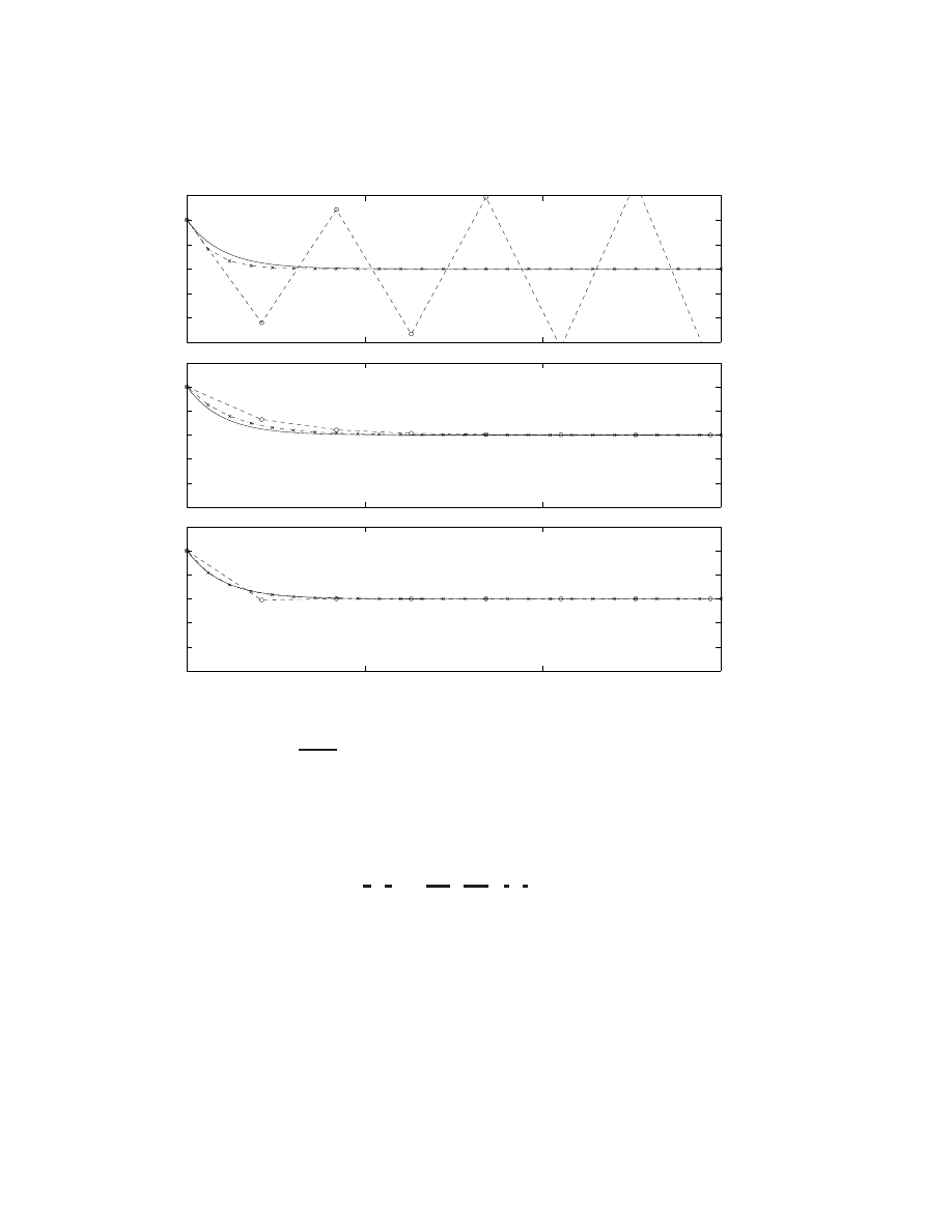
80
CHAPTER
8.
ORDINAR
Y
DIFFERENTIAL
EQUA
TIONS
0
5
10
15
−1.5
−1
−0.5
0
0.5
1
1.5
0
5
10
15
−1.5
−1
−0.5
0
0.5
1
1.5
0
5
10
15
−1.5
−1
−0.5
0
0.5
1
1.5
Figure 8.2: Simulation of the model problem
y
0
=
y
with
=
;
1 using the explicit Euler method
(top), the implicit Euler method (middle), and the trapezoidal method (bottom). Symbols denote:
,
h
= 2
:
1
,
h
= 0
:
6
, exact solution.
We may easily write this second-order ODE as a rst-order system of ODEs by dening
y
1
=
y
and
y
2
=
y
0
and writing:
y
1
y
2
0
|
{z
}
y
0
=
0 1
;
!
2
0
|
{z
}
A
y
1
y
2
|
{z
}
y
:
(8.8)
The eigenvalues of
A
are
i!
. Note that the eigenvalues are imaginary if we has started with the
equation for a damped oscillator, the eigenvalues would have a negative real part as well. Note also
that
A
may be diagonalized by its matrix of eigenvectors:
A
=
S
&
S
;
1
where & =
i!
0
0
;
i!
:
Thus, we have
y
0
=
S
&
S
;
1
y
)
S
;
1
y
0
= &
S
;
1
y
)
z
0
= &
z
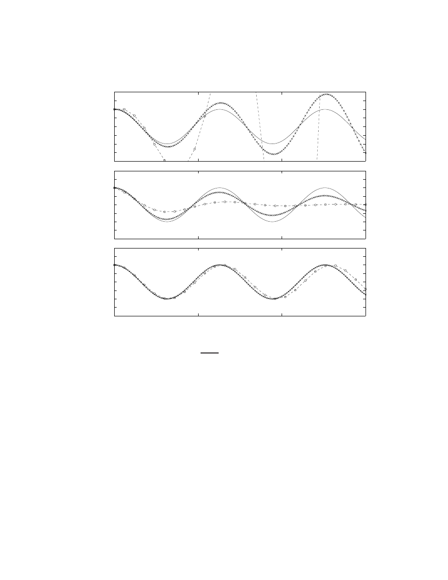
8.3.
A
MODEL
PR
OBLEM
81
0
5
10
15
−2
−1.5
−1
−0.5
0
0.5
1
1.5
2
0
5
10
15
−2
−1.5
−1
−0.5
0
0.5
1
1.5
2
0
5
10
15
−2
−1.5
−1
−0.5
0
0.5
1
1.5
2
Figure 8.3: Simulation of the oscillatory system
y
00
=
;
!
2
y
with
!
= 1 using the explicit Euler
method (top), the implicit Euler method (middle), and the trapezoidal method (bottom). Symbols
denote:
,
h
= 0
:
6
,
h
= 0
:
1
, exact solution.
where we have dened
z
=
S
;
1
y
. In terms of the components of
z
, we have decoupled the dynamics
of the system:
z
0
1
=
i!z
1
z
0
2
=
;
i!z
2
:
Each of these systems is exactly the same form as our scalar model problem (8.6) with complex (in
this case, pure imaginary) values for
. Thus, eigenmode decompositions of physical systems (like
mass/spring systems) motivate us to look at the scalar model problem (8.6) over the complex plane
. In fact, our original second-order system (8.7), as re-expressed in (8.8), will be stable i there are
no eigenvalues of
A
with
<
(
)
>
0.
In Figure 8.3, we show the application of the explicit Euler method, the implicit Euler method,
and the trapezoidal method to the rst-order system of equations (8.8). Note that the explicit Euler
method appears to be unstable for both large and small values of
h
. Note also that all three methods
are more accurate as
h
is rened, with the trapezoidal method appearing to be the most accurate.
We see that some numerical methods for time integration of ODEs are more accurate than others,
and some numerical techniques are sometimes unstable, even for ODEs with stable exact solutions.
82
CHAPTER
8.
ORDINAR
Y
DIFFERENTIAL
EQUA
TIONS
In the next two sections, we develop techniques to quantify both the stability and the accuracy of
numerical methods for time integration of ODEs by application of these numerical methods to the
model problem (8.6).
8.4 Stability
For stability of a numerical method for time integration of an ODE, we want to insure that, if the
exact solution is bounded, the numerical solution is also bounded. We often need to restrict the
timestep
h
in order to insure this. To make this discussion concrete, consider a system whose exact
solution is bounded and dene:
1) a stable numerical scheme: one which does not blow up for any
h
,
2) an unstable numerical scheme: one which blows up for any
h
, and
3) a conditionally stable numerical scheme: one which blows up for some
h
.
8.4.1 Stability of the explicit Euler method
Applying the explicit Euler method (8.3) to the model problem (8.6), we see that
y
n
+1
=
y
n
+
hy
n
= (1 +
h
)
y
n
:
Thus, assuming constant
h
, the solution at time step
n
is:
y
n
= (1 +
h
)
n
y
0
,
n
y
0
)
= 1 +
h:
For large
n
, the numerical solution remains stable i
j
j
1
)
(1 +
R
h
)
2
+ (
I
h
)
2
1
:
The region of the complex plane which satises this stability constraint is shown in Figure 8.4. Note
that this region of stability in the complex plane
h
is consistent with the numerical simulations
shown in Figure 8.2a and 8.3a: for real, negative
, this numerical method is conditionally stable
(i.e., it is stable for suciently small
h
), whereas for pure imaginary
, this numerical method is
unstable for any
h
, though the instability is mild for small
h
.
−4
−3
−2
−1
0
1
2
−3
−2
−1
0
1
2
3
Figure 8.4: Stability of the numerical solution to
y
0
=
y
in the complex plane
h
using the explict
Euler method.
8.4.
ST
ABILITY
83
8.4.2 Stability of the implicit Euler method
Applying the implicit Euler method (8.4) to the model problem (8.6), we see that
y
n
+1
=
y
n
+
hy
n
+1
)
y
n
+1
= (1
;
h
)
;
1
y
n
:
Thus, assuming constant
h
, the solution at time step
n
is:
y
n
=
1
1
;
h
n
y
0
,
n
y
0
)
= 1
1
;
h:
For large
n
, the numerical solution remains stable i
j
j
1
)
(1
;
R
h
)
2
+ (
I
h
)
2
1
:
The region of the complex plane which satises this stability constraint is shown in Figure 8.5. Note
that this region of stability in the complex plane
h
is consistent with the numerical simulations
shown in Figure 8.2b and 8.3b: this method is stable for any stable ODE for any
h
, and is even
stable for some cases in which the ODE itself is unstable.
−4
−3
−2
−1
0
1
2
−3
−2
−1
0
1
2
3
Figure 8.5: Stability of the numerical solution to
y
0
=
y
in the complex plane
h
using the implicit
Euler method.
8.4.3 Stability of the trapezoidal method
Applying the trapezoidal method (8.5) to the model problem (8.6), we see that
y
n
+1
=
y
n
+
h
2 (
y
n
+
y
n
+1
)
)
y
n
+1
=
1 +
h
2
1
;
h
2
!
y
n
:
Thus, assuming constant
h
, the solution at time step
n
is:
y
n
=
1 +
h
2
1
;
h
2
!
n
y
0
,
n
y
0
)
= 1 +
h
2
1
;
h
2
:
For large
n
, the numerical solution remains stable i
j
j
1
)
:::
)
<
(
h
)
0
:
84
CHAPTER
8.
ORDINAR
Y
DIFFERENTIAL
EQUA
TIONS
The region of the complex plane which satises this stability constraint coincides exactly with the
region of stability of the exact solution, as shown in Figure 8.6. Note that this region of stability in
the complex plane
h
is consistent with the numerical simulations shown in Figure 8.2c and 8.3c,
which are stable for systems with
<
(
)
<
0 and marginally stable for systems with
<
(
) = 0.
−4
−3
−2
−1
0
1
2
−3
−2
−1
0
1
2
3
Figure 8.6: Stability of the numerical solution to
y
0
=
y
in the complex plane
h
using the
trapezoidal method.
8.5 Accuracy
Revisiting the model problem
y
0
=
y
, the exact solution (assuming
t
0
= 0 and
h
= constant) is
y
(
t
n
) =
e
t
n
y
0
= (
e
h
)
n
y
0
=
1 +
h
+
2
h
2
2 +
3
h
3
6 +
:::
n
y
0
:
On the other hand, solving the model problem with explicit Euler led to
y
n
= (1 +
h
)
n
y
0
,
n
y
0
solving the model problem with implicit Euler led to
y
n
=
1
1
;
h
n
y
0
=
;
1 +
h
+
2
h
2
+
3
h
3
+
:::
n
y
0
,
n
y
0
and solving the model problem with trapezoidal led to
y
n
=
1 +
h
2
1
;
h
2
!
n
y
0
=
1 +
h
+
2
h
2
2 +
3
h
3
4 +
:::
n
y
0
,
n
y
0
:
To quantify the accuracy of these three methods, we can compare the amplication factor
in each
of the numerical approximations to the exact value
e
h
. The leading order error of the explicit Euler
and implicit Euler methods are seen to be proportional to
h
2
, as noted in
x
8.1, and the leading
order error of the trapezoidal method is proportional to
h
3
. Thus, over a specied time interval
(
t
0
t
0
+
T
),
explicit Euler and implicit Euler are rst-order accurate
and
trapezoidal
is second-order accurate
. The higher order of accuracy of the trapezoidal method implies an
improved rate of convergence of this scheme to the exact solution as the timestep
h
is rened, as
observed in Figures 8.2 and 8.3.

8.6.
R
UNGE-KUTT
A
METHODS
85
8.6 Runge-Kutta methods
An important class of explicit methods, called Runge-Kutta methods, is given by the general form:
k
1
=
f
y
n
t
n
k
2
=
f
y
n
+
1
hk
1
t
n
+
1
h
k
3
=
f
y
n
+
2
hk
1
+
3
hk
2
t
n
+
2
h
...
y
n
+1
=
y
n
+
1
hk
1
+
2
hk
2
+
3
hk
3
+
:::
(8.9)
where the constants
i
,
i
, and
i
are selected to match as many terms as possible of the exact
solution:
y
(
t
n
+1
) =
y
(
t
n
) +
hy
0
(
t
n
) +
h
2
2
y
00
(
t
n
) +
h
3
6
y
0
0 0
(
t
n
) +
:::
where
y
0
=
f
y
00
=
f
t
+
ff
y
y
000
=
f
tt
+
f
t
f
y
+ 2
ff
yt
+
f
2
y
f
+
f
2
f
yy
etc. Runge-Kutta methods are explicit and \self starting", as they don't require any information
about the numerical approximation of the solution before time
t
n
this typically makes them quite
easy to use. As the number of intermediate steps
k
i
in the Runge-Kutta method is increased, the
order of accuracy of the method can also be increased. The stability properties of higher-order
Runge-Kutta methods are also generally quite favorable, as will be shown.
8.6.1 The class of second-order Runge-Kutta methods (RK2)
Consider rst the family of two-step schemes of the form (8.9):
k
1
=
f
(
y
n
t
n
)
k
2
=
f
(
y
n
+
1
hk
1
t
n
+
1
h
)
f
(
y
n
t
n
) +
f
y
(
y
n
t
n
)
1
hf
(
y
n
t
n
)
+
f
t
(
y
n
t
n
)
1
h
y
n
+1
=
y
n
+
1
hk
1
+
2
hk
2
y
n
+
1
hf
(
y
n
t
n
) +
2
h
f
(
y
n
t
n
) +
1
hf
y
(
y
n
t
n
)
f
(
y
n
t
n
) +
1
hf
t
(
y
n
t
n
)
y
n
+ (
1
+
2
)
hf
(
y
n
t
n
) +
2
h
2
1
f
y
(
y
n
t
n
)
f
(
y
n
t
n
) +
2
h
2
1
f
t
(
y
n
t
n
)
:
Note that the approximations given above are exact if
f
is linear in
y
and
t
, as it is in our model
problem. The exact solution we seek to match with this scheme is given by
y
(
t
n
+1
) =
y
(
t
n
) +
hf
(
y
n
t
n
) +
h
2
2
f
t
(
y
n
t
n
) +
f
(
y
n
t
n
)
f
y
(
y
n
t
n
)
+
:::

86
CHAPTER
8.
ORDINAR
Y
DIFFERENTIAL
EQUA
TIONS
Matching coecients to as high an order as possible, we require that
1
+
2
= 1
2
h
2
1
=
h
2
2
2
h
2
1
=
h
2
2
9
>
>
>
>
=
>
>
>
>
)
1
=
1
2
= 1
2
1
1
= 1
;
1
2
1
:
Thus, the general form of the two-step second-order Runge-Kutta method (RK2) is
k
1
=
f
y
n
t
n
k
2
=
f
y
n
+
hk
1
t
n
+
h
y
n
+1
=
y
n
+
1
;
1
2
hk
1
+
1
2
hk
2
(8.10)
where
is a free parameter. A popular choice is
= 1
=
2, which is known as the midpoint method and
has a clear geometric interpretation of approximating a central dierence formula in the integration
of the ODE from
t
n
to
t
n
+1
. Another popular choice is
= 1, which is equivalent to perhaps the
most common so-called \predictor-corrector" scheme, and may be computed in the following order:
predictor :
y
n
+1
=
y
n
+
hf
(
y
n
t
n
)
corrector :
y
n
+1
=
y
n
+
h
2
h
f
(
y
n
t
n
) +
f
(
y
n
+1
t
n
+1
)
i
:
The \predictor" (which is simply an explicit Euler estimate of
y
n
+1
) is only \stepwise 2nd-order
accurate". However, as we shown below, calculation of the \corrector" (which looks roughly like a
recalculation of
y
n
+1
with a trapezoidal rule) results in a value for
y
n
+1
which is \stepwise 3rd-order
accurate" (and thus the scheme is globally 2nd-order accurate).
Applying an RK2 method (for some value of the free parameter
) to the model problem
y
0
=
y
yields
y
n
+1
=
y
n
+
1
;
1
2
hy
n
+
1
2
h
(1 +
h
)
y
n
=
1 +
h
+
2
h
2
2
y
n
,
y
n
)
= 1 +
h
+
2
h
2
2
:
The amplication factor
is seen to be a truncation of the Taylor series of the exact value
e
h
=
1 +
h
+
2
h
2
2
+
3
h
3
6
+
:::
We thus see that the leading order error of this method (for any value
of
) is proportional to
h
3
and, over a specied time interval (
t
0
t
0
+
T
),
an RK2 method is
second-order accurate
. Over a large number of timesteps, the method is stable i
j
j
1 the
domain of stability of this method is illustrated in Figure 8.7.
8.6.
R
UNGE-KUTT
A
METHODS
87
−4
−3
−2
−1
0
1
2
−3
−2
−1
0
1
2
3
Figure 8.7: Stability of the numerical solution to
y
0
=
y
in the complex plane
h
using RK2.
8.6.2 A popular fourth-order Runge-Kutta method (RK4)
The most popular fourth-order Runge-Kutta method is
k
1
=
f
y
n
t
n
k
2
=
f
y
n
+
h
2
k
1
t
n
+1
=
2
k
3
=
f
y
n
+
h
2
k
2
t
n
+1
=
2
k
4
=
f
y
n
+
hk
3
t
n
+1
y
n
+1
=
y
n
+
h
6
k
1
+
h
3
k
2
+
k
3
+
h
6
k
4
(8.11)
This scheme usually performs very well, and is the workhorse of many ODE solvers. This particular
RK4 scheme also has a reasonably-clear geometric interpretation, as discussed further in class.
A derivation similar to that in the previous section conrms that the constants chosen in (8.11)
indeed provide fourth-order accuracy, with the
;
relationship again given by a truncated Taylor
series of the exact value:
= 1 +
h
+
2
h
2
2 +
3
h
3
6 +
4
h
4
24
:
Over a large number of timesteps, the method is stable i
j
j
1 the domain of stability of this
method is illustrated in Figure 8.8.
88
CHAPTER
8.
ORDINAR
Y
DIFFERENTIAL
EQUA
TIONS
−4
−3
−2
−1
0
1
2
−3
−2
−1
0
1
2
3
Figure 8.8: Stability of the numerical solution to
y
0
=
y
in the complex plane
h
using RK4.
8.6.3 An adaptive Runge-Kutta method (RKM4)
Another popular fourth-order scheme, known as the Runge-Kutta-Merson method, is
k
1
=
f
y
n
t
n
k
2
=
f
y
n
+
h
3
k
1
t
n
+1
=
3
k
3
=
f
y
n
+
h
6(
k
1
+
k
2
)
t
n
+1
=
3
k
4
=
f
y
n
+
h
8(
k
1
+ 3
k
3
)
t
n
+1
=
2
y
n
+1
=
y
n
+
h
2
k
1
;
3
h
2
k
3
+ 2
hk
4
k
5
=
f
y
n
+1
t
n
+1
y
n
+1
=
y
n
+
h
6
k
1
+ 2
h
3
k
3
+
h
6
k
5
:
(8.12)
Note that one extra computation of
f
is required in this method as compared with the method given
in (8.11). With the same sort of analysis as we did for RK2, it may be shown that both
y
n
+1
and
y
n
+1
are \stepwise 5th-order accurate", meaning that using either to advance in time over a given
interval gives global 4th-order accuracy. In fact, if ~
y
(
t
) is the exact solution to an ODE and
y
n
takes
this exact value of ~
y
(
t
n
) at
t
=
t
n
, then it follows after a bit of analysis that the errors in
y
n
+1
and
y
n
+1
are
y
n
+1
;
~
y
(
t
n
+1
) =
;
h
5
120 ~
y
(
v
)
+
O
(
h
6
)
(8.13)
y
n
+1
;
~
y
(
t
n
+1
) =
;
h
5
720 ~
y
(
v
)
+
O
(
h
6
)
:
(8.14)
Subtracting (8.13) from (8.14) gives
y
n
+1
;
y
n
+1
=
h
5
144 ~
y
(
v
)
+
O
(
h
6
)
8.6.
R
UNGE-KUTT
A
METHODS
89
which may be substituted on the RHS of (8.14) to give
y
n
+1
;
~
y
(
t
n
+1
) =
;
1
5(
y
n
+1
;
y
n
+1
) +
O
(
h
6
)
:
(8.15)
The quantity on the LHS of (8.15) is the error of our current \best guess" for
y
n
+1
. The rst term
on the RHS is something we can compute, even if we don't know the exact solution ~
y
(
t
). Thus, even
if the exact solution ~
y
(
t
) is unknown, we can still estimate the error of our best guess of
y
n
+1
with
quantities which we have computed. We may use this estimate to decide whether or not to rene
or coarsen the stepsize
h
to attain a desired degree of accuracy on the entire interval. As with the
procedure of adaptive quadrature, it is straightforward to determine whether or not the error on
any particular step is small enough such that, when the entire (global) error is added up, it will be
within a predened acceptable level of tolerance.
8.6.4 A low-storage Runge-Kutta method (RKW3)
Amongst people doing very large simulations with specialized solvers, a third-order scheme which is
rapidly gaining popularity, known as the Runge-Kutta-Wray method, is
k
1
=
f
y
n
t
n
k
2
=
f
y
n
+
1
hk
1
t
n
+
1
h
k
3
=
f
y
n
+
2
hk
1
+
3
hk
2
t
n
+
2
h
y
n
+1
=
y
n
+
1
hk
1
+
2
hk
2
+
3
hk
3
(8.16)
where
1
= 8
=
15
2
= 1
=
4
3
= 5
=
12
1
= 8
=
15
2
= 2
=
3
1
= 1
=
4
2
= 0
3
= 3
=
4
:
−4
−3
−2
−1
0
1
2
−3
−2
−1
0
1
2
3
Figure 8.9: Stability of the numerical solution to
y
0
=
y
in the complex plane
h
using third-order
Runge-Kutta.

90
A derivation similar to that in
x
8.6.1 conrms that the constants chosen in (8.16) indeed provide
third-order accuracy, with the
;
relationship again given by a truncated Taylor series of the
exact value:
= 1 +
h
+
2
h
2
2 +
3
h
3
6
:
Over a large number of timesteps, the method is stable i
j
j
1 the domain of stability of this
method is illustrated in Figure 8.9.
This scheme is particularly useful because it may be computed in the following order
k
1
=
f
y
n
t
n
y
=
y
n
+
1
hk
1
(overwrite
y
n
)
y
=
y
+
1
hk
1
(overwrite
k
1
)
k
2
=
f
y
t
n
+
1
h
(overwrite
y
)
y
=
y
+
3
hk
2
(update
y
)
y
n
+1
=
y
+
2
hk
2
(overwrite
k
2
)
k
3
=
f
y
t
n
+
2
h
(overwrite
y
)
y
n
+1
=
y
n
+1
+
3
hk
3
(update
y
n
+1
)
with
1
=
;
17
=
60 and
2
=
;
5
=
12. Verication that these two forms of the RKW3 scheme are
identical is easily obtained by substitution. The above ordering of the RKW3 scheme is useful when
the dimension
N
of the vector
y
is huge. In the above scheme, we rst compute the vector
k
1
(also of
dimension
N
) as we do, for example, for explicit Euler. However, every operation that follows either
updates an existing vector or may overwrite the memory of an existing vector! (Pointers are very
useful to set up multiple variables at the same memory location.) Thus, we only need enough room
in the computer for two vectors of length
N
, not the four that one might expect are needed upon
examination of (8.16). Amazingly, though this scheme is third-order accurate, it requires no more
memory than explicit Euler. Note that one has to be very careful when computing an operation
like
f
(
y
) in place (i.e., in a manner which immediately overwrites
y
) when the function
f
is a
complicated nonlinear function.
Low-storage schemes such as this are essential in both computational mechanics (e.g., the nite
element modeling of the stresses and temperatures of an engine block) and computational uid
dynamics (e.g., the nite-dierence simulation of the turbulent ow in a jet engine). In these
and many other problems of engineering interest, accurate discretization of the governing PDE
necessitates big state vectors and ecient numerical methods. It is my hope that, in the past
10 weeks, you have begun to get a avor for how such numerical techniques can be derived and
implemented.

App
endix
A
Getting started with Matlab
A.1 What is Matlab?
Matlab, short for Matrix Laboratory, is a high-level language excellent for, among many other things,
linear algebra, data analysis, two and three dimensional graphics, and numerical computation of
small-scale systems. In addition, extensive \toolboxes" are available which contain useful routines
for a wide variety of disciplines, including control design, system identication, optimization, signal
processing, and adaptive lters.
In short, Matlab is a very rapid way to solve problems which don't require intensive compu-
tations or to create plots of functions or data sets. Because a lot of problems encountered in the
engineering world are fairly small, Matlab is an important tool for the engineer to have in his or her
arsenal. Matlab is also useful as a simple programming language in which one can experiment (on
small problems) with ecient numerical algorithms (designed for big problems) in a user-friendly
environment. Problems which do require intensive computations, such as those often encountered
in industry, are more eciently solved in other languages, such as Fortran 90.
A.2 Where to nd Matlab
For those who own a personal computer, the \student edition" of Matlab is available at the bookstore
for just over what it costs to obtain the manual, which is included with the program itself. This is
a bargain price (less than $100) for excellent software, and it is highly recommended that you get
your own (legal) copy of it to take with you when you leave UCSD.
1
For those who don't own a personal computer, or if you choose not to make this investment, you
will nd that Matlab is available on a wide variety of platforms around campus. The most stable
versions are on various Unix machines around campus, including the ACS Unix boxes in the student
labs (accessible by undergrads) and most of the Unix machines in the research groups of the MAE
department. Unix machines running Matlab can be remotely accessed with any computer running
X-windows on campus. There are also several Macs and PCs in the department (including those
run by ACS) with Matlab already loaded.
1
The student edition is actually an almost full-edged version of the latest release of the professional version of
Matlab, limited only in its printing capabilities and the maximum matrix size allowed. Note that the use of m-les
(described at the end of this chapter) allows you to rerun nished Matlab codes at high resolution on the larger Unix
machines to get report-quality printouts, if so desired, after debugging your code on your PC.
1

2
APPENDIX
A.
GETTING
ST
AR
TED
WITH
MA
TLAB
A.3 How to start Matlab
Running Matlab is the same as running any software on the respective platform. For example, on a
Mac or PC, just nd the Matlab icon and double click on it.
Instructions on how to open an account on one of the ACS Unix machines will be discussed in
class. To run Matlab once logged in to one of these machines, just type
matlab
. The PATH variable
should be set correctly so it will start on the rst try|if it doesn't, that machine probably doesn't
have Matlab. If running Matlab remotely, the DISPLAY variable must be set to the local computer
before starting Matlab for the subsequent plots to appear on your screen. For example, if you are
sitting at a machine named turbulence, you need to:
A) log in to turbulence,
B) open a window and telnet to an ACS machine on which you have an account
telnet iacs5
C) once logged in, set the DISPLAY environmental variable, with
setenv DISPLAY turbulence:0.0
D) run Matlab, with
matlab
If you purchase the student edition, of course, full instructions on how to install the program
will be included in the manual.
A.4 How to run Matlab|the basics
Now that you found Matlab and got it running, you are probably on a roll and will stop reading the
manual and this handout (you are, after all, an engineer!) The following section is designed to give
you just enough knowledge of the language to be dangerous. From there, you can:
A) read the manual, available with the student edition or on its own at the bookstore, or
B) use the online help, by typing
help <
command name
>
, for a fairly thorough description of
how any particular command works. Don't be timid to use this approach, as the online help
in Matlab is very extensive.
To begin with, Matlab can function as an ordinary (but expensive!) calculator. At the
>>
prompt,
try typing
>> 1+1
Matlab will reassure you that the universe is still in good order
ans =
2
To enter a matrix, type
>> A = 1 2 3 4 5 6 7 8 0]

A.4.
HO
W
TO
R
UN
MA
TLAB|THE
BASICS
3
Matlab responds with
A =
1
2
3
4
5
6
7
8
0
By default, Matlab operates in an echo mode that is, the elements of a matrix or vector will be
printed out as it is created. This may become tedious for large operations|to suppress it, type a
semicolon after entering commands, such as:
>> A = 1 2 3 4 5 6 7 8 0]
Matrix elements are separated by spaces or commas, and a semicolon indicates the end of a row.
Three periods in a row means that the present command is continued on the following line, as in:
>> A = 1 2 3
...
4 5 6
...
7 8 0]
When typing in a long expression, this can greatly improve the legibility of what you just typed.
Elements of a matrix can also be arithmetic expressions, such as
3*pi
,
5*sqrt(3)
, etc. A column
vector may be constructed with
>> y = 7 8 9]'
resulting in
y =
7
8
9
To automatically build a row vector, a statement such as
>> z = 0:2:10]
results in
z =
0
2
4
6
8
10
Vector
y
can be premultiplied by matrix
A
and the result stored in vector
z
with
>> z = A*y
Multiplication of a vector by a scalar may be accomplished with
>> z = 3.0*y
Matrix A may be transposed as
>> C = A'
The inverse of a matrix is obtained by typing
>> D = inv(A)
A 5
5 identity matrix may be constructed with
>> E = eye(5)
Tridiagonal matrices may be constructed by the following command and variations thereof:
>> 1*diag(ones(m-1,1),-1) - 4*diag(ones(m,1),0) + 1*diag(ones(m-1,1),1)

4
APPENDIX
A.
GETTING
ST
AR
TED
WITH
MA
TLAB
There are two \matrix division" symbols in Matlab,
\
and
/
| if
A
is a nonsingular square
matrix, then
A\B
and
B/A
correspond formally to left and right multiplication of
B
(which must be of
the appropriate size) by the inverse of
A
, that is
inv(A)*B
and
B*inv(A)
, but the result is obtained
directly (via Gaussian elimination with full pivoting) without the computation of the inverse (which
is a very expensive computation). Thus, to solve a system
A*x=b
for the unknown vector
x
, type
>> A=1 2 3 4 5 6 7 8 0]
>> b=5 8 -7]'
>> x=A\b
which results in
x =
-1
0
2
To check this result, just type
>> A*x
which veries that
ans =
5
8
-7
Starting with the innermost group of operations nested in parentheses and working outward, the
usual precedence rules are observed by Matlab. First, all the exponentials are calculated. Then,
all the multiplications and divisions are calculated. Finally, all the additions and subtractions are
calculated. In each of these three catagories, the calculation proceeds from left to right through the
expression. Thus
>> 5/5*3
ans =
3
and
>> 5/(5*3)
ans = 0.3333
It is best to make frequent use of parentheses to insure the order of operations is as you intend.
Note that the matrix sizes must be correct for the requested operations to be dened or an error
will result.
Suppose we have two vectors
x
and
y
and we wish to perform the componentwise operations:
z
=
x
y
for
= 1
n
The Matlab command to execute this is
>> x = 1:5]'
>> y = 6:10]'
>> z = x.*y

A.4.
HO
W
TO
R
UN
MA
TLAB|THE
BASICS
5
Note that
z = x*y
will result in an error, since this implies matrix multiplication and is undened
in this case. (A row vector times a column vector, however, is a well dened operation, so
z = x'*y
is successful. Try it!) The period distinguishes matrix operations (
* ^
and
/
) from component-wise
operations (
.* .^
and
./
). One of the most common bugs when starting out with Matlab is dening
and using row vectors where column vectors are in fact needed.
Matlab also has control ow statements, similar to many programming languages:
>> for i = 1:6, x(i) = i end, x
creates,
x =
1
2
3
4
5
6
Each
for
must be matched by an
end
. Note in this example that commas are used to include several
commands on a single line, and the trailing
x
is used to write the nal value of
x
to the screen. Note
also that this
for
loop builds a row vector, not a column vector. An
if
statement may be used as
follows:
>> n = 7
>> if n > 0, j = 1, elseif n < 0, j = -1, else j = 0, end
The format of a
while
statement is similar to that of the
for
, but exits at the control of a logical
condition:
>> m = 0
>> while m < 7, m = m+2 end, m
Matlab has several advanced matrix functions which will become useful to you as your knowledge
of linear algebra grows. These are summarized in the following section|don't be concerned if most
of these functions are unfamiliar to you now. One command which we will encounter early in the
quarter is LU decomposition:
>> A=1 2 3 4 5 6 7 8 0]
>> L,U,P]=lu(A)
This results in a lower triangular matrix
L
, an upper triangular matrix
U
, and a permutation matrix
P
such that
P*X = L*U
L =
1.0000
0
0
0.1429
1.0000
0
0.5714
0.5000
1.0000
U =
7.0000
8.0000
0
0
0.8571
3.0000
0
0
4.5000
P =
0
0
1
1
0
0
0
1
0

6
APPENDIX
A.
GETTING
ST
AR
TED
WITH
MA
TLAB
Checking this with
>> P\L*U
conrms that the original matrix
A
is recovered.
A.5 Commands for matrix factoring and decomposition
The following commands are but a small subset of what Matlab has to oer:
>> R = chol(X)
produces an upper triangular
R
so that
R'*R = X
. If
X
is not positive denite, an error message is
printed.
>> V,D] = eig(X)
produces a diagonal matrix
D
of eigenvalues and a full matrix
V
whose columns are the corresponding
eigenvectors so that
X*V = V*D
.
>> p = poly(A)
If
A
is an N by N matrix,
poly(A)
is a row vector with N+1 elements which are the coecients of
the characteristic polynomial,
det(lambda*eye(A) - A)
.
If
A
is a vector,
poly(A)
is a vector whose elements are the coecients of the polynomial whose
roots are the elements of
A
.
>> P,H] = hess(A)
produces a unitary matrix
P
and a Hessenberg matrix
H
so that
A = P*H*P'
and
P'*P = eye(size(P))
.
>> L,U,P] = lu(X)
produces a lower triangular matrix
L
, an upper triangular matrix
U
, and a permutation matrix
P
so
that
P*X = L*U
.
>> Q = orth(A)
produces an orthonormal basis for the range of
A
. Note that
Q'*Q = I
, the columns of
Q
span the
same space as the columns of
A
and the number of columns of
Q
is the rank of
A
.
>> Q,R] = qr(X)
produces an upper triangular matrix
R
of the same dimension as
X
and a unitary matrix
Q
so that
X = Q*R
.
>> U,S,V] = svd(X)
produces a diagonal matrix S, of the same dimension as
X
, with nonnegative diagonal elements in
decreasing order, and unitary matrices
U
and
V
so that
X = U*S*V'
.
A.6.
COMMANDS
USED
IN
PLOTTING
7
A.6 Commands used in plotting
For a two dimensional plot, try for example:
>> x=0:.1:10]
>> y1=sin(x)
>> y2=cos(x)
>> plot(x,y1,'-',x,y2,'x')
This results in the plot:
0
1
2
3
4
5
6
7
8
9
10
−1
−0.8
−0.6
−0.4
−0.2
0
0.2
0.4
0.6
0.8
1
Three dimensional plots are also possible:
>> x,y] = meshgrid(-8:.5:8,-8:.5:8)
>> R = sqrt(x.^2 + y.^2) + eps
>> Z = sin(R)./R
>> mesh(Z)
0
10
20
30
40
0
10
20
30
40
−0.4
−0.2
0
0.2
0.4
0.6
0.8
1
This results in the plot:
Axis rescaling and labelling can be controlled with
loglog
,
semilogx
,
semilogy
,
title
,
xlabel
,
and
ylabel
|see the help pages for more information.

8
APPENDIX
A.
GETTING
ST
AR
TED
WITH
MA
TLAB
A.7 Other Matlab commands
Typing
who
lists all the variables created up to that point. Typing
whos
gives detailed information
showing sizes of arrays and vectors.
In order to save the entire variable set computed in a session, type
save session
prior to
quitting. All variables will be saved in a le named session.mat. At a later time the session may be
resumed by typing
load session
. Save and load commands are menu-driven on the Mac and PC.
Some additional useful functions, which are for the most part self-explanatory (check the help
page if not), are:
abs, conj, sin, cos, tan, asin, acos, atan, sinh, cosh, tanh, exp,
log, log10, eps
.
Matlab also has many special functions built in to aid in linear problem-solving an index of
these along with their usage is in the Matlab manual. Note that many of the `built-in' functions are
just prewritten m-les stored in subdirectories, and can easily be opened and accessed by the user
for examination.
A.8 Hardcopies
Hardcopies of graphs on the Unix stations are best achieved using the
command. This creates
postscript les which may then be sent directly to a postscript printer using the local print command
(usually
lp
or
lpr
) at the Unix level. If using the
-deps
option of the
command in Matlab,
then the encapulated postscript le (e.g.,
figure1.eps
) may be included in TEX documents as done
here.
Hardcopies of graphs on a Mac may be obtained from the options available under the `File' menu.
On the student edition for the PC, the
prtscr
command may be used for a screen dump.
Text hardcopy on all platforms is best achieved by copying the text in the Matlab window and
pasting it in to the editor of your choosing and then printing from there.
A.9 Matlab programming procedures: m-les
In addition to the interactive, or \Command" mode, you can execute a series of Matlab commands
that are stored in `m-les', which have a le extension `.m'. An example m-le is shown in the
following section. When working on more complicated problems, it is a very good idea to work from
m-les so that set-up commands don't need to be retyped repeatedly.
Any text editor may be used to generate m-les. It is important to note that these should be plain
ASCI text les|type in the sequence of commands exactly as you would if running interactively.
The
%
symbol is used in these les to indicate that the rest of that line is a comment|comment all m-
les clearly, suciently, and succinctly, so that you can come back to the code later and understand
how it works. To execute the commands in an m-le called sample.m, simply type
sample
at the
Matlab
>>
prompt. Note that an m-le may call other m-les. Note that there are two types of
m-les: scripts and functions. A script is just a list of matlab commands which run just as if you
had typed them in one at a time (though it sounds pedestrian, this simple method is a useful and
straightforward mode of operation in Matlab). A function is a set of commands that is \called" (as
in a real programming language), only inheriting those variables in the argument list with which it
is called and only returning the variables specied in the function declaration. These two types of
m-les will be illustrated thoroughly by example as the course proceeds.
On Unix machines, Matlab should be started from the directory containing your m-les so that
Matlab can nd these les. On all platforms, I recommend making a new directory for each new
problem you work on, to keep things organized and to keep from overwriting previously-written

A.10.
SAMPLE
M-FILE
9
m-les. On the Mac and the PC, the search path must be updated using the
path
command after
starting Matlab so that Matlab can nd your m-les (see help page for details).
A.10 Sample m-le
% sample.m
echo on, clc
% This code uses MATLAB's eig program to find eigenvalues of
% a few random matrices which we will construct with special
% structure.
%
% press any key to begin
pause
R = rand(4)
eig(R)
% As R has random entries, it may have real or complex eigenvalues.
% press any key
pause
eig(R + R')
% Notice that R + R' is symmetric, with real eigenvalues.
% press any key
pause
eig(R - R')
% The matrix R - R' is skew-symmetric, with imaginary eigenvalues.
% press any key
pause
V,D] = eig(R'*R)
% This matrix R'*R is symmetric, with real POSITIVE eigenvalues.
% press any key
pause
V,D] = eig(R*R')
% R*R' has the same eigenvalues as R'*R. But different eigenvectors!
% press any key
pause
% You can create matrices with desired eigenvalues 1,2,3,4 from any
% invertible S times lambda times S inverse.
S = rand(4)
lambda = diag(1 2 3 4])
A = S * lambda * inv(S)
eig(A)
echo off
% end sample.m
Wyszukiwarka
Podobne podstrony:
Numerical methods in sci and eng
Numerical methods in sci and eng
Numerical Methods for Engineers and Scientists, 2nd Edition
Improvements in Fan Performance Rating Methods for Air and Sound
Little Daniel Objectivity Truth and Method in Anthropology
Improvements in Fan Performance Rating Methods for Air and Sound
PSYCHIC METHODS OF DIAGNOSIS AND TREATMENT IN ACUPUNCTURE …
Estimation of Dietary Pb and Cd Intake from Pb and Cd in blood and urine
automating with step 7 in lad and fbd simatic (1)
Key Concepts in Language and Linguistics
Guide to the properties and uses of detergents in biology and biochemistry
2008 4 JUL Emerging and Reemerging Viruses in Dogs and Cats
2002 3 MAY Lasers in Medicine and Surgery
In vivo MR spectroscopy in diagnosis and research of
conceptual storage in bilinguals and its?fects on creativi
20090602 01 ANSF, Coalition Forces further disable IED?lls in Khowst and Zabul
Methods in Enzymology 463 2009 Quantitation of Protein
więcej podobnych podstron