
Electronic Journal of Differential Equations, Monograph 05, 2004.
ISSN: 1072-6691. URL: http://ejde.math.txstate.edu or http://ejde.math.unt.edu
ftp ejde.math.txstate.edu (login: ftp)
SINGULARITIES OF TRANSITION PROCESSES IN
DYNAMICAL SYSTEMS: QUALITATIVE THEORY OF
CRITICAL DELAYS
ALEXANDER N. GORBAN
Abstract. This monograph presents a systematic analysis of the singularities
in the transition processes for dynamical systems. We study general dynamical
systems, with dependence on a parameter, and construct relaxation times that
depend on three variables: Initial conditions, parameters k of the system,
and accuracy ε of the relaxation.
We study the singularities of relaxation
times as functions of (x
0
, k) under fixed ε, and then classify the bifurcations
(explosions) of limit sets. We study the relationship between singularities of
relaxation times and bifurcations of limit sets. An analogue of the Smale order
for general dynamical systems under perturbations is constructed. It is shown
that the perturbations simplify the situation: the interrelations between the
singularities of relaxation times and other peculiarities of dynamics for general
dynamical system under small perturbations are the same as for the Morse-
Smale systems.
Contents
2
Bifurcations (Explosions) of ω-limit Sets
11
Extension of Semiflows to the Left
11
13
Convergence in the Spaces of Sets
14
16
20
20
Slow Relaxations and Bifurcations of ω-limit Sets
23
Slow Relaxations of One Semiflow
29
29
Slow Relaxations and Stability
30
Slow Relaxations in Smooth Systems
33
Slow Relaxation of Perturbed Systems
35
35
2000 Mathematics Subject Classification. 54H20, 58D30, 37B25.
Key words and phrases. Dynamical system; transition process; relaxation time; bifurcation;
limit set; Smale order.
c
2004 Texas State University - San Marcos.
Submitted May 29, 2004. Published August 7, 2004.
1
2
A. N. GORBAN
EJDE-2004/MON. 05
41
Smale Order and Smale Diagram for General Dynamical Systems
45
Slow Relaxations in One Perturbed System
49
51
52
Introduction
Are there “white spots” in topological dynamics? Undoubtedly, they exist: The
transition processes in dynamical systems are still not very well known.
As a
consequence, it is difficult to interpret the experiments that reveal singularities of
transition processes, and in particular, anomalously slow relaxation. “Anomalously
slow” means here “unexpectedly slow”; but what can one expect from a dynamical
system in a general case?
In this monograph, we study the transition processes in general dynamical sys-
tems. The approach based on the topological dynamics is quite general, but one
pays for these generality by the loss of constructivity. Nevertheless, this stage of a
general consideration is needed.
The limiting behaviour (as t → ∞) of dynamical systems have been studied
very intensively in the XX century [16, 37, 36, 68, 12, 56]. New types of limit
sets (“strange attractors”) were discovered [50, 1]. Fundamental results concerning
the structure of limit sets were obtained, such as the Kolmogorov–Arnold–Moser
theory [11, 55], the Pugh lemma [61], the qualitative [66, 47, 68] and quantitative
[38, 79, 40] Kupka–Smale theorem, etc. The theory of limit behaviour “on the
average”, the ergodic theory [45], was considerably developed. Theoretical and
applied achievements of the bifurcation theory have become obvious [3, 13, 60].
The fundamental textbook on dynamical systems [39] and the introductory review
[42] are now available.
The achievements regarding transition processes have not been so impressive,
and only relaxations in linear and linearized systems are well known. The appli-
cations of this elementary theory received the name the “relaxation spectroscopy”.
Development of this discipline with applications in chemistry and physics was dis-
tinguished by Nobel Prize (M. Eigen [24]).
A general theory of transition processes of essentially non-linear systems does not
exist. We encountered this problem while studying transition processes in catalytic
reactions. It was necessary to give an interpretation on anomalously long transition
processes observed in experiments. To this point, a discussion arose and even some
papers were published. The focus of the discussion was: do the slow relaxations
arise from slow “strange processes” (diffusion, phase transitions, and so on), or
could they have a purely kinetic (that is dynamic) nature?
Since a general theory of relaxation times and their singularities was not available
at that time, we constructed it by ourselves from the very beginning [35, 34, 32, 33,
25, 30]. In the present paper the first, topological part of this theory is presented.
It is quite elementary theory, though rather lengthy ε − δ reasonings may require
some time and effort. Some examples of slow relaxation in chemical systems, their
theoretical and numerical analysis, and also an elementary introduction into the
theory can be found in the monograph [78].

EJDE-2004/MON. 05
SINGULARITIES OF TRANSITION PROCESSES
3
Two simplest mechanisms of slow relaxations can be readily mentioned: The
delay of motion near an unstable fixed point, and the delay of motion in a domain
where a fixed point appears under a small change of parameters. Let us give some
simple examples of motion in the segment [−1, 1].
The delay near an unstable fixed point exists in the system ˙
x = x
2
− 1. There
are two fixed points x = ±1 on the segment [−1, 1], the point x = 1 is unstable and
the point x = −1 is stable. The equation is integrable explicitly:
x = [(1 + x
0
)e
−t
− (1 − x
0
)e
t
]/[(1 + x
0
)e
−t
+ (1 − x
0
)e
t
],
where x
0
= x(0) is initial condition at t = 0. If x
0
6= 1 then, after some time, the
motion will come into the ε-neighborhood of the point x = −1, for whatever ε > 0.
This process requires the time
τ (ε, x
0
) = −
1
2
ln
ε
2 − ε
−
1
2
ln
1 − x
0
1 + x
0
.
It is assumed that 1 > x
0
> ε − 1. If ε is fixed then τ tends to +∞ as x
0
→ 1
like −
1
2
ln(1 − x
0
). The motion that begins near the point x = 1 remains near this
point for a long time (∼ −
1
2
ln(1 − x
0
)), and then goes to the point x = −1. In
order to show it more clear, let us compute the time τ
0
of residing in the segment
[−1 + ε, 1 − ε] of the motion, beginning near the point x = 1, i.e. the time of its
stay outside the ε-neighborhoods of fixed points x = ±1. Assuming 1 − x
0
< ε, we
obtain
τ
0
(ε, x
0
) = τ (ε, x
0
) − τ (2 − ε, x
0
) = − ln
ε
2 − ε
.
One can see that if 1 − x
0
< ε then τ
0
(ε, x
0
) does not depend on x
0
. This is obvious:
the time τ
0
is the time of travel from point 1 − ε to point −1 + ε.
Let us consider the system ˙
x = (k + x
2
)(x
2
− 1) on [−1, 1] and try to obtain an
example of delay of motion in a domain where a fixed point appears under small
change of parameter. If k > 0, there are again only two fixed points x = ±1,
x = −1 is a stable point and x = 1 is an unstable. If k = 0 there appears the
third point x = 0. It is not stable, but “semistable” in the following sense: If the
initial position is x
0
> 0 then the motion goes from x
0
to x = 0. If x
0
< 0 then the
motion goes from x
0
to x = −1. If k < 0 then apart from x = ±1, there are two
other fixed points x = ±
p|k|. The positive point is stable, and the negative point
is unstable. Let us consider the case k > 0. The time of motion from the point x
0
to the point x
1
can be found explicitly (x
0,1
6= ±1):
t =
1
2
ln
1 − x
1
1 + x
1
−
1
2
ln
1 − x
0
1 + x
0
−
1
√
k
arctan
x
1
√
k
− arctan
x
0
√
k
.
If x
0
> 0, x
1
< 0, k > 0, k → 0, then t → ∞ like π/
√
k. These examples do not
exhaust all the possibilities; they rather illustrate two common mechanisms of slow
relaxations appearance.
Below we study parameter-dependent dynamical systems. The point of view of
topological dynamics is adopted (see [16, 37, 36, 56, 65, 80]). In the first place this
means that, as a rule, the properties associated with the smoothness, analyticity
and so on will be of no importance. The phase space X and the parameter space
K are compact metric spaces: for any points x
1
, x
2
from X (k
1
, k
2
from K) the

4
A. N. GORBAN
EJDE-2004/MON. 05
distance ρ(x
1
, x
2
) (ρ
K
(k
1
, k
2
)) is defined with the following properties:
ρ(x
1
, x
2
) = ρ(x
2
, x
1
),
ρ(x
1
, x
2
) + ρ(x
2
, x
3
) ≥ ρ(x
1
, x
3
),
ρ(x
1
, x
2
) = 0 if and only if x
1
= x
2
(similarly for ρ
K
).
The sequence x
i
converges to x
∗
(x
i
→ x
∗
) if ρ(x
i
, x
∗
) → 0. The compactness
means that from any sequence a convergent subsequence can be chosen.
The states of the system are represented by the points of the phase space X. The
reader can think of X and K as closed, bounded subsets of finite-dimensional Eu-
clidean spaces, for example polyhedrons, and ρ and ρ
K
are the standard Euclidean
distances.
Let us define the phase flow (the transformation “shift over the time t”). It
is a function f of three arguments: x ∈ X (of the initial condition), k ∈ K (the
parameter value) and t ≥ 0, with values in X: f (t, x, k) ∈ X. This function is
assumed continuous on [0, ∞) × X × K and satisfying the following conditions:
• f (0, x, k) = x (shift over zero time leaves any point in its place);
• f (t, f (t
0
, x, k), k) = f (t + t
0
, x, k) (the result of sequentially executed shifts
over t and t
0
is the shift over t + t
0
);
• if x 6= x
0
, then f (t, x, k) 6= f (t, x
0
, k) (for any t distinct initial points are
shifted in time t into distinct points for.
For a given parameter value k ∈ K and an initial state x ∈ X, the ω-limit set
ω(x, k) is the set of all limit points of f (t, x, k) as t → ∞:
y is in ω(x, k) if and only if there exists a sequence t
i
≥ 0 such that
t
i
→ ∞ and f (t
i
, x, k) → y.
Examples of ω-limit points are stationary (fixed) points, points of limit cycles and
so on.
The relaxation of a system can be understood as its motion to the ω-limit set
corresponding to given initial state and value of parameter. The relaxation time
can be defined as the time of this motion. However, there are several possibilities
to make this definition precise.
Let ε > 0. For given value of parameter k we denote by τ
1
(x, k, ε) the time
during which the system will come from the initial state x into the ε-neighbourhood
of ω(x, k) (for the first time). The (x, k)-motion can enter the ε-neighborhood of
the ω-limit set, then this motion can leave it, then reenter it, and so on it can
enter and leave the ε-neighbourhood of ω(x, k) several times. After all, the motion
will enter this neighbourhood finally, but this may take more time than the first
entry. Therefore, let us introduce for the (x, k)-motion the time of being outside
the ε-neighborhood of ω(x, k) (τ
2
) and the time of final entry into it (τ
3
). Thus, we
have a system of relaxation times that describes the relaxation of the (x, k)-motion
to its ω-limit set ω(x, k):
τ
1
(x, k, ε) = inf{t > 0 : ρ
∗
(f (t, x, k), ω(x, k)) < ε};
τ
2
(x, k, ε) = meas{t > 0 : ρ
∗
(f (t, x, k), ω(x, k)) ≥ ε};
τ
3
(x, k, ε) = inf{t > 0 : ρ
∗
(f (t
0
, x, k), ω(x, k)) < ε for t
0
> t}.
Here meas is the Lebesgue measure (on the real line it is length), ρ
∗
is the distance
from the point to the set: ρ
∗
(x, P ) = inf
y∈P
ρ(x, y).

EJDE-2004/MON. 05
SINGULARITIES OF TRANSITION PROCESSES
5
The ω-limit set depends on an initial state (even under the fixed value of k).
The limit behavior of the system can be characterized also by the total limit set
ω(k) =
[
x∈X
ω(x, k).
The set ω(k) is the union of all ω(x, k) under given k. Whatever initial state would
be, the system after some time will be in the ε-neighborhood of ω(k). The relaxation
can be also considered as a motion towards ω(k). Introduce the corresponding
system of relaxation times:
η
1
(x, k, ε) = inf{t > 0 : ρ
∗
(f (t, x, k), ω(k)) < ε};
η
2
(x, k, ε) = meas{t > 0 : ρ
∗
(f (t, x, k), ω(k)) ≥ ε};
η
3
(x, k, ε) = inf{t > 0 : ρ
∗
(f (t
0
, x, k), ω(k)) < ε for t
0
> t}.
Now we are able to define a slow transition process. There is no distinguished
scale of time, which could be compared with relaxation times. Moreover, by de-
crease of the relaxation accuracy ε the relaxation times can become of any large
amount even in the simplest situations of motion to unique stable fixed point. For
every initial state x and given k and ε all relaxation times are finite. But the set
of relaxation time values for various x and k and given ε > 0 can be unbounded.
Just in this case we speak about the slow relaxations.
Let us consider the simplest example. Let us consider the differential equation
˙
x = x
2
− 1 on the segment [−1, 1]. The point x = −1 is stable, the point x = 1
is unstable. For any fixed ε > 0, ε <
1
2
the relaxation times τ
1,2,3
, η
3
have the
singularity: τ
1,2,3
, η
3
(x, k, ε) → ∞ as x → 1, x < 1. The times η
1
, η
2
remain
bounded in this case.
Let us say that the system has τ
i
- (η
i
)-slow relaxations, if for some ε > 0 the
function τ
i
(x, k, ε) (η
i
(x, k, ε)) is unbounded from above in X × K, i.e. for any t > 0
there are such x ∈ X, k ∈ K, that τ
i
(x, k, ε) > t (η
i
(x, k, ε) > t).
One of the possible reasons of slow relaxations is a sudden jump in dependence
of the ω-limit set ω(x, k) of x, k (as well as a jump in dependence of ω(k) of k).
These “explosions” (or bifurcations) of ω-limit sets are studied in Sec. 1. In the
next Sec. 2 we give the theorems, providing necessary and sufficient conditions of
slow relaxations. Let us mention two of them.
Theorem 2.9
. A system has τ
1
-slow relaxations if and only if there is a singularity
on the dependence ω(x, k) of the following kind: There exist points x
∗
∈ X, k
∗
∈ K,
sequences x
i
→ x
∗
, k
i
→ k
∗
, and number δ > 0, such that for any i, y ∈ ω(x
∗
, k
∗
),
z ∈ ω(x
i
, k
i
) the distance satisfies ρ(y, z) > δ.
The singularity of ω(x, k) described in the statement of the theorem indicates
that the ω-limit set ω(x, k) makes a jump: the distance from any point of ω(x
i
, k
i
)
to any point of ω(x
∗
, k
∗
) is greater than δ.
By the next theorem, necessary and sufficient conditions of τ
3
-slow relaxations
are given. Since τ
3
≥ τ
1
, the conditions of τ
3
-slow relaxations are weaker than the
conditions of Theorem 2.9
, and τ
3
-slow relaxations are “more often” than τ
1
-slow
relaxation (the relations between different kinds of slow relaxations with corre-
sponding examples are given below in Subsec. 3.2). That is why the discontinuities
of ω-limit sets in the following theorem are weaker.
6
A. N. GORBAN
EJDE-2004/MON. 05
Theorem 2.20. τ
3
-slow relaxations exist if and only if at least one of the following
conditions is satisfied:
(1) There are points x
∗
∈ X, k
∗
∈ K, y
∗
∈ ω(x
∗
, k
∗
), sequences x
i
→ x
∗
,
k
i
→ k
∗
and number δ > 0 such that for any i and z ∈ ω(x
i
, k
i
) the
inequality ρ(y
∗
, z) > δ is valid (The existence of one such y is sufficient,
compare it with Theorem 2.9
).
(2) There are x ∈ X, k ∈ K such that x 6∈ ω(x, k), for any t > 0 can be found
y(t) ∈ X, for which f (t, y(t), k) = x (y(t) is a shift of x over −t), and for
some z ∈ ω(x, k) can be found such a sequence t
i
→ ∞ that y(t
i
) → z.
That is, the (x, k)-trajectory is a generalized loop: the intersection of its
ω-limit set and α-limit set (i.e., the limit set for t → −∞) is non-empty,
and x is not a limit point for the (x, k)-motion.
An example of the point satisfying the condition 2 is provided by any point lying
on the loop, that is the trajectory starting from the fixed point and returning to
the same point.
Other theorems of Sec. 2 also establish connections between slow relaxations and
peculiarities of the limit behaviour under different initial conditions and parameter
values. In general, in topological and differential dynamics the main attention is
paid to the limit behavior of dynamical systems [16, 37, 36, 68, 12, 56, 65, 80, 57,
41, 18, 39, 42]. In applications, however, it is often of importance how rapidly the
motion approaches the limit regime. In chemistry, long-time delay of reactions far
from equilibrium (induction periods) have been studied since Van’t-Hoff [73] (the
first Nobel Prize laureate in Chemistry). It is necessary to mention the classical
monograph of N.N. Semjonov [30] (also the Nobel Prize laureate in Chemistry),
where induction periods in combustion are studied. From the latest works let us
note [69]. When minimizing functions by relaxation methods, the similar delays can
cause some problems. The paper [29], for example, deals with their elimination.
In the simplest cases, the slow relaxations are bound with delays near unstable
fixed points. In the general case, there is a complicated system of interrelations
between different types of slow relaxations and other dynamical peculiarities, as
well as of different types of slow relaxations between themselves. These relations
are the subject of Sects. 2, 3. The investigation is performed generally in the way
of classic topological dynamics [16, 37, 36]. There are, however, some distinctions:
• From the very beginning not only one system is considered, but also prac-
tically more important case of parameter dependent systems;
• The motion in these systems is defined, generally speaking, only for positive
times.
The last circumstance is bound with the fact that for applications (in particular,
for chemical ones) the motion is defined only in a positively invariant set (in balance
polyhedron, for example). Some results can be accepted for the case of general
semidynamical systems [72, 14, 54, 70, 20], however, for the majority of applications,
the considered degree of generality is more than sufficient.
For a separate semiflow f (without parameter) η
1
-slow relaxations are impos-
sible, but η
2
-slow relaxations can appear in a separate system too (Example 2.4).
Theorem 3.2 gives the necessary conditions for η
2
-slow relaxations in systems with-
out parameter.

EJDE-2004/MON. 05
SINGULARITIES OF TRANSITION PROCESSES
7
Let us recall the definition of non-wandering points. A point x
∗
∈ X is the
non-wandering point for the semiflow f , if for any neighbourhood U of x
∗
and for
any T > 0 there is such t > T that f (t, U )
T U 6= ∅. Let us denote by ω
f
the
complete ω-limit set of one semiflow f (instead of ω(k)).
Theorem 3.2. Let a semiflow f possess η
2
-slow relaxations. Then there exists a
non-wandering point x
∗
∈ X which does not belong to ω
f
.
For of smooth systems it is possible to obtain results that have no analogy in
topological dynamics. Thus, it is shown in Sec. 2 that “almost always” η
2
-slow re-
laxations are absent in one separately taken C
1
-smooth dynamical system (system,
given by differential equations with C
1
-smooth right parts). Let us explain what
“almost always” means in this case. A set Q of C
1
-smooth dynamical systems with
common phase space is called nowhere-dense in C
1
-topology, if for any system from
Q an infinitesimal perturbation of right hand parts can be chosen (perturbation of
right hand parts and its first derivatives should be smaller than an arbitrary given
ε > 0) such that the perturbed system should not belong to Q and should exist
ε
1
> 0 (ε
1
< ε) such that under ε
1
-small variations of right parts (and of first
derivatives) the perturbed system could not return in Q. The union of finite num-
ber of nowhere-dense sets is also nowhere-dense. It is not the case for countable
union: for example, a point on a line forms nowhere-dense set, but the countable set
of rational numbers is dense on the real line: a rational number is on any segment.
However, both on line and in many other cases countable union of nowhere-dense
sets (the sets of first category) can be considered as very “meagre”. Its comple-
ment is so-called “residual set”. In particular, for C
1
-smooth dynamical systems
on compact phase space the union of countable number of nowhere-dense sets has
the following property: any system, belonging to this union, can be eliminated from
it by infinitesimal perturbation. The above words “almost always” meant: except
for union of countable number of nowhere-dense sets.
In two-dimensional case (two variables), “almost any” C
1
-smooth dynamical
system is rough, i.e. its phase portrait under small perturbations is only slightly
deformed, qualitatively remaining the same. For rough two-dimensional systems
ω-limit sets consist of fixed points and limit cycles, and the stability of these points
and cycles can be verified by linear approximation. The correlation of six different
kinds of slow relaxations between themselves for rough two-dimensional systems
becomes considerably more simple.
Theorem 3.12. Let M be C
∞
-smooth compact manifold, dim M = 2, F be a
structural stable smooth dynamical system over M , F |
X
be an associated with M
semiflow over connected compact positively invariant subset X ⊂ M . Then:
(1) For F |
X
the existence of τ
3
-slow relaxations is equivalent to the existence
of τ
1,2
- and η
3
-slow relaxations;
(2) F |
X
does not possess τ
3
-slow relaxations if and only if ω
F
T X consists of
one fixed point or of points of one limit cycle;
(3) η
1,2
-slow relaxations are impossible for F |
X
.
For smooth rough two-dimensional systems it is easy to estimate the measure
(area) of the region of durable delays µ
i
(t) = meas{x ∈ X : τ
i
(x, ε) > t} under
fixed sufficiently small ε and large t (the parameter k is absent because a separate
system is studied). Asymptotical behaviour of µ
i
(t) as t → ∞ does not depend on

8
A. N. GORBAN
EJDE-2004/MON. 05
i and
lim
t→∞
ln µ
i
(t)
t
= − min{κ
1
, . . . , κ
n
},
where n is a number of unstable limit motions (of fixed points and cycles) in X,
and the numbers are determined as follows. We denote by B
i
, . . . , B
n
the unstable
limit motions lying in X.
(1) Let B
i
be an unstable node or focus. Then κ
1
is the trace of matrix of
linear approximation in the point b
i
.
(2) Let b
i
be a saddle. Then κ
1
is positive eigenvalue of the matrix of linear
approximation in this point.
(3) Let b
i
be an unstable limit cycle. Then κ
i
is characteristic indicator of the
cycle (see [15, p. 111]).
Thus, the area of the region of initial conditions, which result in durable delay of
the motion, in the case of smooth rough two-dimensional systems behaves at large
delay times as exp(−κt), where t is a time of delay, κ is the smallest number of
κ
i
, . . . , κ
n
. If κ is close to zero (the system is close to bifurcation [12, 15]), then
this area decreases slowly enough at large t. One can find here analogy with linear
time of relaxation to a stable fixed point
τ
l
= −1/ max Reλ
where λ runs through all the eigenvalues of the matrix of linear approximation of
right parts in this point, max Reλ is the largest (the smallest by value) real part of
eigenvalue, τ
l
→ ∞ as Reλ → 0.
However, there are essential differences. In particular, τ
l
comprises the eigen-
values (with negative real part) of linear approximation matrix in that (stable)
point, to which the motion is going, and the asymptotical estimate µ
i
comprises
the eigenvalues (with positive real part) of the matrix in that (unstable) point or
cycle, near which the motion is retarded.
In typical situations for two-dimensional parameter depending systems the singu-
larity of τ
l
entails existence of singularities of relaxation times τ
i
(to this statement
can be given an exact meaning and it can be proved as a theorem). The inverse
is not true. As an example should be noted the delays of motions near unstable
fixed points. Besides, for systems of higher dimensions the situation becomes more
complicated, the rough systems cease to be “typical” (this was shown by S. Smale
[67], the discussion see in [12]), and the limit behaviour even of rough systems does
not come to tending of motion to fixed point or limit cycle. Therefore the area
of reasonable application the linear relaxation time τ
l
to analysis of transitional
processes becomes in this case even more restricted.
Any real system exists under the permanent perturbing influence of the external
world.
It is hardly possible to construct a model taking into account all such
perturbations. Besides that, the model describes the internal properties of the
system only approximately.
The discrepancy between the real system and the
model arising from these two circumstances is different for different models. So, for
the systems of celestial mechanics it can be done very small. Quite the contrary, for
chemical kinetics, especially for kinetics of heterogeneous catalysis, this discrepancy
can be if not too large but, however, not such small to be neglected. Strange as
it may seem, the presence of such an unpredictable divergence of the model and
reality can simplify the situation: The perturbations “conceal” some fine details of
dynamics, therefore these details become irrelevant to analysis of real systems.
EJDE-2004/MON. 05
SINGULARITIES OF TRANSITION PROCESSES
9
Sec. 4 is devoted to the problems of slow relaxations in presence of small pertur-
bations. As a model of perturbed motion here are taken ε-motions: the function of
time ϕ(t) with values in X, defined at t ≥ 0, is called ε-motion (ε > 0) under given
value of k ∈ K, if for any t ≥ 0, τ ∈ [0, T ] the inequality ρ(ϕ(t+τ ), f (τ, ϕ(t), k)) < ε
holds. In other words, if for an arbitrary point ϕ(t) one considers its motion on the
force of dynamical system, this motion will diverge ϕ(t + τ ) from no more than at
ε for τ ∈ [0, T ]. Here [0, T ] is a certain interval of time, its length T is not very
important (it is important that it is fixed), because later we shall consider the case
ε → 0.
There are two traditional approaches to the consideration of perturbed motions.
One of them is to investigate the motion in the presence of small constantly acting
perturbations [22, 51, 28, 46, 52, 71, 53], the other is the study of fluctuations
under the influence of small stochastic perturbations [59, 74, 75, 43, 44, 76]. The
stated results join the first direction, but some ideas bound with the second one are
also used. The ε-motions were studied earlier in differential dynamics, in general
in connection with the theory of Anosov about ε-trajectories and its applications
[41, 6, 77, 26, 27], see also [23].
When studying perturbed motions, we correspond to each point “a bundle” of
ε-motions, {ϕ(t)}, t ≥ 0 going out from this point (ϕ(0) = x) under given value of
parameter k. The totality of all ω-limit points of these ε-motions (of limit points
of all ϕ(t) as t → ∞) is denoted by ω
ε
(x, k). Firstly, it is necessary to notice that
ω
ε
(x, k) does not always tend to ω(x, k) as ε → 0: the set ω
0
(x, k) =
T
ε>0
ω
ε
(x, k)
may not coincide with ω(x, k). In Sec. 4 there are studied relaxation times of ε-
motions and corresponding slow relaxations. In contrast to the case of nonperturbed
motion, all natural kinds of slow relaxations are not considered because they are
too numerous (eighteen), and the principal attention is paid to two of them, which
are analyzed in more details than in Sec. 2.
The structure of limit sets of one perturbed system is studied. The analogy
of general perturbed systems and Morse-Smale systems as well as smooth rough
two-dimensional systems is revealed. Let us quote in this connection the review by
Professor A. M. Molchanov of the thesis [31] of A. N. Gorban
(1981):
After classic works of Andronov, devoted to the rough systems on
the plane, for a long time it seemed that division of plane into finite
number of cells with source and drain is an example of structure
of multidimensional systems too... The most interesting (in the
opinion of opponent) is the fourth chapter “Slow relaxations of the
perturbed systems”. Its principal result is approximately as follows.
If a complicated dynamical system is made rough (by means of ε-
motions), then some its important properties are similar to the
properties of rough systems on the plane. This is quite positive
result, showing in what sense the approach of Andronov can be
generalized for arbitrary systems.
To study limit sets of perturbed system, two relations are introduced in [30] for
general dynamical systems: the preorder % and the equivalence ∼:
• x
1
% x
2
if for any ε > 0 there is such a ε-motion ϕ(t) that ϕ(0) = x
1
and
ϕ(τ ) = x
2
for some τ > 0;
1
This paper is the first complete publication of that thesis.
10
A. N. GORBAN
EJDE-2004/MON. 05
• x
1
∼ x
2
if x
1
% x
2
and x
2
% x
1
.
For smooth dynamical systems with finite number of “basic attractors” similar
relation of equivalence had been introduced with the help of action functionals in
studies on stochastic perturbations of dynamical systems ([76] p. 222 and further).
The concepts of ε-motions and related topics can be found in [23]. For the Morse-
Smale systems this relation is the Smale order [68].
Let ω
0
=
S
x∈X
ω
0
(x) (k is omitted, because only one system is studied). Let us
identify equivalent points in ω
0
. The obtained factor-space is totally disconnected
(each point possessing a fundamental system of neighborhoods open and closed
simultaneously). Just this space ω
0
/ ∼ with the order over it can be considered as a
system of sources and drains analogous to the system of limit cycles and fixed points
of smooth rough two-dimensional dynamical system. The sets ω
0
(x) can change by
jump only on the boundaries of the region of attraction of corresponding “drains”
(Theorem 4.43). This totally disconnected factor-space ω
0
/ ∼ is the generalization
of the Smale diagrams [68] defined for the Morse-Smale systems onto the whole
class of general dynamical systems. The interrelation of six principal kinds of slow
relaxations in perturbed system is analogous to their interrelation in smooth rough
two-dimensional system described in Theorem 3.12.
Let us enumerate the most important results of the investigations being stated.
(1) It is not always necessary to search for “foreign” reasons of slow relaxations,
in the first place one should investigate if there are slow relaxations of
dynamical origin in the system.
(2) One of possible reasons of slow relaxations is the existence of bifurcations
(explosions) of ω-limit sets. Here, it is necessary to study the dependence
ω(x, k) of limit set both on parameters and initial data. It is violation of
the continuity with respect to (x, k) ∈ X × K that leads to slow relaxations.
(3) The complicated dynamics can be made “rough” by perturbations. The use-
ful model of perturbations in topological dynamics provide the ε-motions.
For ε → 0 we obtain the rough structure of sources and drains similar to the
Morse-Smale systems (with totally disconnected compact instead of finite
set of attractors).
(4) The interrelations between the singularities of relaxation times and other
peculiarities of dynamics for general dynamical system under small pertur-
bations are the same as for the Morse-Smale systems, and, in particular,
the same as for rough two-dimensional systems.
(5) There is a large quantity of different slow relaxations, unreducible to each
other, therefore for interpretation of experiment it is important to under-
stand which namely of relaxation times is large.
(6) Slow relaxations in real systems often are “bounded slow”, the relaxation
time is large (essentially greater than could be expected proceeding from
the coefficients of equations and notions about the characteristic times),
but nevertheless bounded. When studying such singularities, appears to
be useful the following method, ascending to the works of A.A. Andronov:
the considered system is included in appropriate family for which slow re-
laxations are to be studied in the sense accepted in the present work. This
study together with the mention of degree of proximity of particular sys-
tems to the initial one can give an important information.

EJDE-2004/MON. 05
SINGULARITIES OF TRANSITION PROCESSES
11
1. Bifurcations (Explosions) of ω-limit Sets
Let X be a compact metric space with the metrics ρ, and K be a compact metric
space (the space of parameters) with the metrics ρ
K
,
f : [0, ∞) × X × K → X
(1.1)
be a continuous mapping for any t ≥ 0, k ∈ K; let mapping f (t, ·, k) : X →
X be homeomorphism of X into subset of X and under every k ∈ K let these
homeomorphisms form monoparametric semigroup:
f (0, ·, k) = id, f (t, f (t
0
, x, k), k) = f (t + t
0
, x, k)
(1.2)
for any t, t
0
≥ 0, x ∈ X.
Below we call the semigroup of mappings f (t, ·, k) under fixed k a semiflow
of homeomorphisms (or, for short, semiflow), and the mapping (1.1) a family of
semiflows or simply a system (1.1). It is obvious that all results, concerning the
system (1.1), are valid also in the case when X is a phase space of dynamical system,
i.e. when every semiflow can be prolonged along t to the left onto the whole axis
(−∞, ∞) up to flow (to monoparametric group of homeomorphisms of X onto X).
1.1. Extension of Semiflows to the Left. It is clear that for fixed x and k the
mapping f (·, x, k): t → f (t, x, k) can be, generally speaking, defined also for certain
negative t, preserving semigroup property (1.2). In fact, for fixed x and k consider
the set of all non-negative t for which there is point q
i
∈ X such that f (t, q
i
, k) = x.
Let us denote the upper bound of this set by T (x, k):
T (x, k) = sup{t : ∃q
t
∈ X, f (t, q
t
, k) = x}.
(1.3)
For given t, x, k the point q
t
, if it exists, has a single value, since the mapping
f (t, ·, k) : X → X is homeomorphism. Introduce the notation f (−t, x, k) = q
t
. If
f (−t, x, k) is determined, then for any τ within 0 ≤ τ ≤ t the point f (−τ, x, k)
is determined: f (−τ, x, k) = f (t − τ, f (−t, x, k), k). Let T (x, k) < ∞,
T (x, k) >
t
n
> 0
(n = 1, 2, . . . ),
t
n
→ T . Let us choose from the sequence f (−t
n
, x, k)
a subsequence converging to some q
∗
∈ X and denote it by {q
j
}, and the corre-
sponding times denote by −t
j
(q
j
= f (−t
j
, x, k)). Owing to the continuity of f
we obtain: f (t
j
, q
j
, k) → f (T (x, k), q
∗
, k), therefore f (T (x, k), q
∗
, k) = x. Thus,
f (−T (x, k), x, k) = q
∗
.
So, for fixed x, k the mapping f was determined in interval [−T (x, k), ∞), if
T (x, k) is finite, and in (−∞, ∞) in the opposite case. Let us denote by S the set
of all triplets (t, x, k), in which f is now determined. For enlarged mapping f the
semigroup property in following form is valid:
Proposition 1.1 (Enlarged semigroup property).
(A) If (τ, x, k) and (t, f (τ, x, k), k) ∈ S, then (t + τ, x, k) ∈ S and
f (t, f (t, x, k), k) = f (t + τ, x, k) .
(1.4)
(B) Simmilarly, if (t + τ, x, k) and (τ, x, k) ∈ S, then (t, f (τ, x, k), k) ∈ S and
(1.4) holds.
Thus, if the left part of the equality (1.4) makes sense, then its right part is also
determined and the equation is valid. If there are determined both the right part
and f (τ, x, k) in the left part, then the whole left part makes sense and (1.4) hold.

12
A. N. GORBAN
EJDE-2004/MON. 05
Proof. We consider several possible cases. Since the parameter k is fixed, for short
notation, it is omitted in the formulas.
Case (1)
f (t, f (−τ, x)) = f (t − τ, x)
(t, τ > 0);
case (a) t > τ > 0.
Let the left part make sense, i.e., f (−τ, x) is determined. Then, taking into account
that t − τ > 0, we have
f (t, f (−τ, x)) = f (t − τ + τ, f (−τ, x)) = f (t − τ, f (τ, f (−τ, x))) = f (t − τ, x),
since f (τ, f (−τ, x)) = x by definition. Therefore, the equality is true (the right part
makes sense since t > τ )- the part for the case 1a is proved. Similarly, if f (−τ, x) is
determined, then the whole left part (t > 0) makes sense, and then according to the
proved the equality is true. The other cases are considered in analogous way.
Proposition 1.2. The set S is closed in (−∞, ∞) × X × K and the mapping
f : S → X is continuous.
Proof. Denote by h−T (x, k), ∞) the interval [−T (x, k), ∞), if T (x, k) is finite, and
the whole axis (−∞, ∞) in opposite case. Let t
n
→ t
∗
, x
n
→ x
∗
, k
n
→ k
∗
, and
t
n
∈ h−T (x
n
, k
n
), ∞). To prove the proposition, it should be made certain that t
∗
∈
h−T (x
∗
, k
∗
), ∞) and f (t
n
, x
n
, k
n
) → f (t
∗
, x
∗
, k
∗
). If t
∗
> 0, this follows from the
continuity of f in [0, ∞) × X × K. Let t
∗
≤ 0. Then it can be supposed that t
n
< 0.
Let us re-denote by changing the signs t
n
by −t
n
and t
∗
by −t
∗
. Let us choose from
the sequence f (−t
n
, x
n
, k
n
) using the compactness of X a subsequence converging
to some q
∗
∈ X. let us denote it by q
j
, and the sequences of corresponding t
n
, x
n
and k
n
denote by t
j
, x
j
and k
j
. The sequence f (t
j
, q
j
, k
j
) converges to f (t
∗
, q
∗
, k
∗
)
(t
j
> 0, t
∗
> 0). But f (t
j
, q
j
, k
j
) = x
j
→ x
∗
. That is why f (t
∗
, q
∗
, k
∗
) = x
∗
and f (−t
∗
, x
∗
, k
∗
) = q
∗
is determined. Since q
∗
is an arbitrary limit point of {q
n
},
and the point f (−t
∗
, x
∗
, k
∗
), if it exists, is determined by given t
∗
, x
∗
, k
∗
and has a
single value, the sequence q
n
converges to q
∗
. The proposition is proved.
Later on we shall call the mapping f (·, x, k) : h−T (x, k), ω) → X k-motion of
the point x ((k, x)-motion), the image of (k, x)-motion – k-trajectory of the point
x ((k, x)-trajectory), the image of the interval h−T (x, k), 0) a negative, and the
image of 0, ∞) a positive k-semitrajectory of the point x ((k, x)-semitrajectory). If
T (x, k) = ∞, then let us call the k-motion of the point x the whole k-motion, and
the corresponding k-trajectory the whole k-trajectory.
Let (x
n
, k
n
) → (x
∗
, k
∗
), t
n
→ t
∗
, t
n
, t
∗
> 0 and for any n the (k
n
, x
n
)-motion
be determined in the interval [−t
n
, ∞), i.e. [−t
n
, ∞) ⊂ h−T (x
n
, k
n
), ∞). Then
(k
∗
, x
∗
)-motion is determined in [−t
∗
, ∞]. In particular, if all (k
n
, x
n
)-motions are
determined in [−¯
t, ∞) (¯
t > 0), then (k
∗
, x
∗
)-motion is determined in too. If t
n
→ ∞
and (k
n
, x
n
)-motion is determined in [−t
n
, ∞), then (k
∗
, x
∗
)-motion is determined
in (−∞, ∞) and is a whole motion. In particular, if all the (k
n
, x
n
)-motions are
whole, then (k
∗
, x
∗
)-motion is whole too. All this is a direct consequence of the
closure of the set S, i.e. of the domain of definition of extended mapping f . It
should be noted that from (x
n
, k
n
) → (x
∗
, k
∗
) and [−t
∗
, ∞) ⊂ h−T (x
∗
, k
∗
), ∞)
does not follow that for any ε > 0 [−t
∗
+ ε, ∞) ⊂ h−T (x
n
, k
n
), ∞) for n large
enough.
Let us note an important property of uniform convergence in compact inter-
vals. Let (x
n
, k
n
) → (x
∗
, k
∗
) and all (k
n
, x
n
)-motions and correspondingly (k
∗
, x
∗
)-
motion be determined in compact interval [a, b]. Then (k
n
, x
n
)-motions converge

EJDE-2004/MON. 05
SINGULARITIES OF TRANSITION PROCESSES
13
uniformly in [a, b] to (k
∗
, x
∗
)-motion: f (t, x
n
, k
n
) ⇒ f (t, x
∗
, k
∗
). This is a direct
consequence of continuity of the mapping f : S → X
1.2. Limit Sets.
Definition 1.3. Point p ∈ X is called ω- (α-)-limit point of the (k, x)-motion (corre-
spondingly of the whole (k, x)-motion), if there is such sequence t
n
→ ∞ (t
n
→ −∞)
that f (t
n
, x, k) → p as n → ∞. The totality of all ω- (α-)-limit points of (k, x)-
motion is called its ω- (α-)-limit set and is denoted by ω(x, k) (α(x, k)).
Definition 1.4. A set W ⊂ X is called k-invariant set, if for any x ∈ W the
(k, x)-motion is whole and the whole (k, x)-trajectory belongs W . In similar way,
let us call a set V ⊂ X (k, +)-invariant ((k,positively)-invariant), if for any x ∈ V ,
t > 0, f (t, x, k) ∈ V .
Proposition 1.5. The sets ω(x, k) and α(x, k) are k-invariant.
Proof. Let p ∈ ω(x, k), t
n
→ ∞, x
n
= f (t
n
, x, k) → p. Note that (k, x
n
)-motion
is determined at least in [−t
n
, ∞). Therefore, as it was noted above, (k, p)-motion
is determined in (−∞, ∞), i.e. it is whole. Let us show that the whole (k, p)-
trajectory consists of ω-limit points of (k, x)-motion. Let f (¯
t, p, k) be an arbitrary
point of (k, p)-trajectory. Since t → ∞, from some nis determined a sequence
f (¯
t + t
n
, x, k)). It converges to f (¯
t, p, k), since f (¯
t + t
n
, x, k) = f (¯
t, f (t
n
, x, k), k)
(according to Proposition 1.1), f (t
n
, x, k) → p and f : S → X is continuous
(Proposition 1.2).
Now, let q ∈ α(x, k), t
n
→ −∞ and x
n
= f (t
n
, x, k) → q. Since (according
to the definition of α-limit points) (k, x)-motion is whole, then all (k, x
n
)-motions
are whole too. Therefore, as it was noted, (k, q)-motion is whole. Let us show
that every point f (¯
t, q, k) of (k, q)-trajectory is α-limit for (k, x)-motion. Since
(k, x)-motion is whole, then the semigroup property and continuity of f in S give
f (¯
t + t
n
, x, k) = f (¯
t, f (t
n
, x, k), k) → f (¯
t, q, k),
and since ¯
t + t
n
→ −∞, then f (¯
t, q, k) is α-limit point of (k, x)-motion. Proposition
1.5 is proved.
Further we need also the complete ω-limit set ω(k) : ω(k) =
S
x∈X
ω(x, k). The
set ω(k) is k-invariant, since it is the union of k-invariant sets.
Proposition 1.6. The sets ω(x, k), α(x, k) (the last in the case when (k, x)-motion
is whole) are nonempty, closed and connected.
The proof practically coincides with the proof of similar statements for usual
dynamical systems ([56, p.356-362]). The set ω(k) might not be closed.
Example 1.7 (The set ω(k) might not be closed). Let us consider the system given
by the equations ˙
x = y(x − 1), ˙
y = −x(x − 1) in the circle x
2
+ y
2
≤ 1 on the plane.
The complete ω-limit set is ω = {(1, 0)}
S{(x, y) : x
2
+ y
2
< 1}. It is unclosed.
The closure of ω coincides with the whole circle (x
2
+ y
2
≤ 1), the boundary
of ω consists of two trajectories: of the fixed point (1, 0) ∈ ω and of the loop
{(x, y) : x
2
+ y
2
= 1, x 6= 1} * ω
Proposition 1.8. The sets ∂ω(k), ∂ω(k) \ ω(k) and ∂ω(k)
T ω(k) are (k, +)-
invariant. Furthermore, if ∂ω(k) \ ω(k) 6= ∅, then ∂ω(k)
T ω(k) 6= ∅ (∂ω(k) =
ω(k) \ intω(k) is the boundary of the set ω(k)).

14
A. N. GORBAN
EJDE-2004/MON. 05
Let us note that for the propositions 1.6 and 1.8 to be true, the compactness of X
is important, because for non-compact spaces analogous propositions are incorrect,
generally speaking.
To study slow relaxations, we need also sets that consist of ω-limit sets ω(x, k)
as of elements (the sets of ω-limit sets):
Ω(x, k) = {ω(x
0
, k) : ω(x
0
, k) ⊂ ω(x, k), x
0
∈ X};
Ω(k) = {ω(x, k) : x ∈ X},
(1.5)
where Ω(x, k) is the set of all ω-limit sets, lying in ω(x, k), Ω(k) is the set of ω-limit
sets of all k-motions.
1.3. Convergence in the Spaces of Sets. Further we consider the connec-
tion between slow relaxations and violations of continuity of the dependencies
ω(x, k), ω(k), Ω(x, k), Ω(k). Let us introduce convergences in spaces of sets and in-
vestigate the mappings continuous with respect to them. One notion of continuity,
used by us, is well known (see [48, Sec. 18] and [49, Sec. 43] lower semicontinuity).
Two other ones are some more “exotic”. In order to reveal the resemblance and
distinctions between these convergences, let us consider them simultaneously (all
the statements, concerning lower semicontinuity, are variations of known ones, see
[48, 49]).
Let us denote the set of all nonempty subsets of X by B(X), and the set of all
nonempty subsets of B(X) by B(B(X)).
Let us introduce in B(X) the following proximity measures: let p, q ∈ B(X),
then
d(p, q) = sup
x∈p
inf
y∈q
ρ(x, y);
(1.6)
r(p, q) =
inf
x∈p,y∈q
ρ(x, y).
(1.7)
The “distance” d(p, q) represents “a half” of the known Hausdorff metrics ([49,
p.223]):
dist(p, q) = max{d(p, q), d(q, p)}.
(1.8)
It should be noted that, in general, d(p, q) 6= d(q, p). Let us determine in B(X)
converges using the introduced proximity measures. Let q
n
be a sequence of points
of B(X). We say that q
n
d-converges to p ∈ B(X), if d(p, q
n
) → 0. Analogously,
q
n
r-converges to p ∈ B(X), if r(p, q
n
) → 0. Let us notice that d-convergence
defines topology in B(X) with a countable base in every point and the continuity
with respect to this topology is equivalent to d-continuity (λ-topology [48, p.183]).
As a basis of neighborhoods of the point p ∈ B(X) in this topology can be taken,
for example, the family of sets {q ∈ B(X) : d(p, q) < 1/n (n = 1, 2, . . . )}. The
topology conditions can be easily verified, since the triangle inequality
d(p, s) ≤ d(p, q) + d(q, s)
(1.9)
is true (in regard to these conditions see, for example, [19, p.19-20]), r-convergence
does not determine topology in B(X).
To prove this, let us use the following
obvious property of convergence in topological spaces: if p
i
≡ p, q
i
≡ q and s
i
≡ s
are constant sequences of the points of topological space and p
i
→ q, q
i
→ s, then
p
i
→ s. This property is not valid for r-convergence. To construct an example,
it is enough to take two points x, y ∈ X (x 6= y) and to make p = {x}, q =
{x, y}, s = {y}. Then r(p, q) = r(q, s) = 0, r(p, s) = ρ(x, y) > 0. Therefore

EJDE-2004/MON. 05
SINGULARITIES OF TRANSITION PROCESSES
15
p
i
→ q, q
i
→ s, p
i
6→ s, and r-convergence does not determine topology for any
metric space X 6= {x}.
Introduce also a proximity measure in B(B(X)) (that is the set of nonempty
subsets of B(X)): let P, Q ∈ B(B(X)), then
D(P, Q) = sup
p∈P
inf
q∈Q
r(p, q).
(1.10)
Note that the formula (1.10) is similar to the formula (1.6), but in (1.10) appears
r(p, q) instead of ρ(x, y). The expression (1.10) can be somewhat simplified by
introducing the following denotations. Let Q ∈ B(B(X)). Let us define SQ =
S
q∈Q
q, SQ ∈ B(X); then
D(P, Q) = sup
p∈P
r(p, SQ).
(1.11)
Let us introduce convergence in B(B(X)) (D-convergence):
Q
n
→ P, if D(P, Q
n
) → 0.
D-convergence, as well as r-convergence, does not determine topology. This can
be illustrated in the way similar to that used for r-convergence. Let x, y ∈ X,
x 6= y, P = {{x}}, Q = {{x, y}}, R = {{y}}, P
i
= P , Q
i
= Q. Then D(Q, P ) =
D(R, Q) = 0, P
i
→ Q, Q
i
→ R, D(R, P ) = ρ(x, y) > 0, P
i
6→ R.
Later we need the following criteria of convergence of sequences in B(X) and in
B(B(X)).
Proposition 1.9 ([48]). The sequence of sets q
n
∈ B(X) d-converges to p ∈ B(X)
if and only if inf
y∈q
n
ρ(x, y) → 0 as n → ∞ for any x ∈ p.
Proposition 1.10. The sequence of sets q
n
∈ B(X) r-converges to p ∈ B(X) if
and only if there are such x
n
∈ p and y
n
∈ q
n
that ρ(x
n
, y
n
) → 0 as n → ∞.
This follows immediately from the definition of r-proximity. Before treating the
criterion of D-convergence, let us prove the following topological lemma.
Lemma 1.11. Let p
n
, q
n
(n = 1, 2, . . . ) be subsets of compact metric space X and
r(p
n
, q
n
) > ε > 0 for any n. Then there are such γ > 0 and an infinite set of
indices J that r(p
N
, q
n
) > γ for n ∈ J and for some number N .
Proof. Choose in X ε/5-network M ; let to each q ⊂ X correspond q
M
⊂ M :
q
M
=
m ∈ M
inf
x∈q
ρ(x, m) ≤ ε/5
.
(1.12)
For any two sets p, q ⊂ X r(p
M
, q
M
) +
2
5
ε ≥ r(p, q). Therefore r(p
M
n
, q
M
n
) > 3ε/5.
Since the number of different pairs p
M
, q
M
is finite (M is finite), there exists an
infinite set J of indices n, for which the pairs p
M
n
, q
M
n
coincide: p
M
n
= p
M
, q
M
n
= q
M
as n ∈ J . For any two indices n, l ∈ J r(p
M
n
, q
M
l
) = r(p
M
, q
M
) > 3ε/5, therefore
r(p
n
, q
l
) > ε/5, and this fact completes the proof of the lemma. It was proved more
important statement really: there exists such infinite set J of indices that for any
n, l ∈ J r(p
n
, q
l
) > γ (and not only for one N ).
Proposition 1.12. The sequence of sets Q
n
∈ B(B(X)) D-converges to p ∈ B(X))
if and only if inf
q∈Q
r(p, q) → 0 for any p ∈ P .

16
A. N. GORBAN
EJDE-2004/MON. 05
Proof. In one direction this is obvious: if Q
n
→ P , then according to definition
D(P, Q
n
) → 0, i.e. the upper bound by p ∈ P of the value inf
q∈Q
n
r(p, q) tends
to zero and all the more for any p ∈ P inf
q∈Q
r(p, q) → 0. Now, suppose that
for any p ∈ P inf
q∈Q
n
r(p, q) → 0. If D(P, Q
n
) 6→ 0, then one can consider that
D(P, Q
n
) > ε > 0. Therefore (because of (1.11)) there are such p
n
∈ P for which
r(p
n
, SQ
n
) > ε SQ
n
=
S
q∈Q
n
q
. Using Lemma 1.11, we conclude that for some
N r(p
N
, SQ
n
) > γ > 0, i.e. inf
q∈Q
n
r(p
N
, q) 6→ 0. The obtained contradiction
proves the second part of Proposition 1.12.
For the rest of this monograph, if not stated otherwise, the convergence in B(X)
implies d-convergence, and the convergence in B(B(X)) implies D-convergence,
and as continuous are considered the functions with respect to these convergences.
1.4. Bifurcations of ω-limit Sets.
Definition 1.13. We say that the system (1.1) possesses:
(A) ω(x, k)-bifurcations, if ω(x, k) is not continuous function in X × K;
(B) ω(k)-bifurcations, if ω(k) is not continuous function in K;
(C) Ω(x, k)-bifurcations, if Ω(x, k) is not continuous function in X × K;
(D) Ω(k)-bifurcations, if Ω(k) is not continuous function in K.
The points of X × K or K, in which the functions ω(x, k), ω(k), Ω(x, k), Ω(k)
are not d- or not D-continuous, we call the points of bifurcation. The considered
discontinuities in the dependencies ω(x, k), ω(k), Ω(x, k), Ω(k) could be also called
“explosions” of ω-limit sets (compare with the explosion of the set of non-wandering
points in differential dynamics ([57], Sec. 6.3., p.185-192, which, however, is a vio-
lation of semidiscontinuity from above).
Proposition 1.14.
(A) If the system (1.1) possesses Ω(k)-bifurcations, then it
possesses Ω(x, k)-, ω(x, k)- and ω(x, k)-bifurcations.
(B) If the system (1.1) possesses Ω(x, k)-bifurcations, then it possesses ω(x, k)-
bifurcations.
(C) If the system (1.1) possesses ω(k)-bifurcations, then it possesses ω(x, k)-
bifurcations.
It is convenient to illustrate Proposition 1.14 by the scheme (the word “bifurca-
tion” is omitted):
?
Ω(k)
?
Ω(x, k)
ω(k)
-
ω(x, k)
(1.13)
Proof. Let us begin from item C. Let the system (1.1) (family of semiflows) possess
ω(k)-bifurcations. This means that there are such k
∗
∈ K (point of bifurcation),
ε > 0, x
∗
∈ ω(k
∗
) and sequence k
n
∈ K, k
n
→ k
∗
, for which inf
y∈ω(x
0
,k
n
)
ρ(x
∗
, y) >
ε for any n (according to Proposition 1.9). The point x
∗
belongs to some ω(x
0
, k
∗
)
(x
0
∈ X). Note that ω(x
0
, k
n
) ⊂ ω(k
n
), consequently, inf
y∈ω(k
n
)
ρ(x
∗
, y) > ε,
therefore the sequence ω(x
0
, k
n
) does not converge to ω(x
0
, k
∗
): there exist ω(x, k)-
bifurcations, and the point of bifurcation is (x
0
, k
∗
).
Prove the statement in item B. Let the system (1.1) possess Ω(x, k)-bifurcations.
Then, (according to Proposition 1.12) there are such (x
∗
, k
∗
) ∈ X × K (the point
of bifurcation), ω(x
0
, k
∗
) ⊂ ω(x
∗
, k
∗
) and sequence (x
n
, k
n
) → (x
∗
, k
∗
) that
r(ω(x
0
, k
∗
), S Ω(x
n
, k
n
)) > ε > 0
for any n.

EJDE-2004/MON. 05
SINGULARITIES OF TRANSITION PROCESSES
17
But the above statement implies r(ω(s
0
, k
∗
), ω(x
n
, k
n
)) > ε > 0 and, consequently,
inf
y∈ω(x
n
,k
n
)
ρ(ξ, y) > ε
for any ξ ∈ ω(x
0
, k
∗
).
Since ξ ∈ ω(x
∗
, k
∗
), the existence of ω(x, k)-bifurcations follows and (x
∗
, k
∗
) is the
point of bifurcation.
Statement in item A. Let the system (1.1) possess Ω(k)-bifurcations. Then there
are k
∗
∈ K (the point of bifurcation), ε > 0 and sequence of points k
n
, k
n
→ k
∗
,
for which D(Ω(k
∗
), Ω(k
n
)) > ε for any n, that is for any n there is such x
n
∈ X
that r(ω(x
n
, k
∗
), ω(k
n
)) > ε (according to (1.11)). By Lemma 1.11 there are such
γ > 0 and a natural N that for infinite set J of indices r(ω(x
N
, k
∗
), ω(k
n
)) > γ for
n ∈ J . Furthermore, r(ω(x
N
, k
∗
), ω(x
N
, k
n
)) > γ (n ∈ J ), consequently, there are
Ω(x, k)-bifurcations:
(x
N
, k
n
) → (x
N
, k
∗
)
as n → ∞, n ∈ J ;
D(Ω(x
N
, k
∗
), Ω(x
N
, k
n
)) =
sup
ω(x,k
∗
)⊂Ω(x
N
,k
∗
)
r(ω(x, k
∗
), ω(x
N
, k
n
))
≥ r(ω(x
N
, k
∗
), ω(x
N
, k
n
)) > γ.
Therefore, the point of bifurcation is (x
N
, k
∗
).
We need to show only that if there are Ω(k)-bifurcations, then ω(k)-bifurcations
exist. Let us prove this. Let the system (1.1) possess Ω(k)-bifurcations. Then, as
it was shown just above, there are such k
∗
∈ K, x
∗
∈ X, γ > 0 (x
∗
= x
N
) and a
sequence of points k
n
∈ K that k
n
→ k
∗
and r(ω(x
∗
, k
∗
), ω(k
n
)) > γ. Furthermore,
for any ξ ∈ ω(x
∗
, k
∗
), inf
y∈ω(k
n
)
ρ(ξ, y) > γ; therefore d(ω(k
∗
), ω(k
n
)) > γ and
there are ω(k)-bifurcations (k
∗
is the point of bifurcation). Proposition 1.14 is
proved.
Proposition 1.15. The system (1.1) possesses Ω(x, k)-bifurcations if and only if
ω(x, k) is not r-continuous function in X × K.
Proof. Let the system (1.1) possess Ω(x, k)-bifurcations, then there are (x
∗
, k
∗
) ∈
X × K, the sequence (x
n
, k
n
) ∈ X × K, (x
n
, k
n
) → (x
∗
, k
∗
) for which for any n,
D(Ω(x
∗
, k
∗
), Ω(x
n
, k
n
)) > ε > 0.
The last means that for any n there is x
∗
n
∈ X for which ω(x
∗
n
, k
∗
) ⊂ ω(x
∗
, k
∗
),
and r(ω(x
∗
n
, k
∗
), ω(x
n
, k
n
)) > ε. ¿From Lemma 1.11 follows the existence of such
γ > 0 and natural N that for infinite set J of indices r(ω(x
∗
N
, k
∗
), ω(x
n
, k
n
)) > γ as
n ∈ J . Let x
∗
0
be an arbitrary point of ω(x
∗
N
, k
∗
). As it was noted already, (k
∗
, x
∗
0
)-
trajectory lies in ω(x
∗
N
< k
∗
) and because of the closure of the last ω(x
∗
0
, k
∗
) ⊂
ω(x
∗
N
, k
∗
). Therefore, r(ω(x
n
, k
n
)) > γ as n ∈ J . As x
∗
0
∈ ω(x
∗
, k
∗
), there is such
sequence t
i
→ ∞, t
i
> 0, that f (t
i
, x
∗
, k
∗
) → x
∗
0
as i → ∞. Using the continuity
of f , choose for every i such n(i) ∈ J that ρ(f (t
i
, x
∗
, k
∗
), f (t
i
, x
n(i)
, k
n(i)
)) < 1/i.
Denote f (t
i
, x
n(i)
, k
n(i)
) = x
0
i
, k
n(i)
= k
0
i
. Note that ω(x
0
i
, k
0
i
) = ω(x
n(i)
, k
n(i)
).
Therefore, for any i r(ω(x
∗
0
, k
∗
), ω(x
0
i
, k
0
i
)) > γ. Since (x
0
i
, k
0
i
) → (x
∗
0
, k
∗
), we con-
clude that ω(x, k) is not r-continuous function in X × K.
Let us emphasize that the point of Ω(x, k)-bifurcations can be not the point of
r-discontinuity.
Now, suppose that ω(x, k) is not r-continuous in X × K.
Then there exist
(x
∗
, k
∗
) ∈ X × K, sequence of points (x
n
, k
n
) ∈ X × K, (x
n
, k
n
) → (x
∗
, k
∗
), and
ε > 0, for which r(ω(x
∗
, k
∗
), ω(x
n
, k
n
)) > ε for any n. But, according to (1.11),
18
A. N. GORBAN
EJDE-2004/MON. 05
from this it follows that D(Ω(x
∗
, k
∗
), Ω(x
n
, k
n
)) > ε for any n. Therefore, (x
∗
, k
∗
)
is the point of Ω(x, k)-bifurcation. Proposition 1.15 is proved.
The ω(k)- and ω(x, k)-bifurcations can be called bifurcations with appearance of
new ω-limit points, and Ω(k)- and Ω(x, k)-bifurcations with appearance of ω-limit
sets. In the first case there is such sequence of points k
n
(or (x
n
, k
n
)), converging to
the point of bifurcation k
∗
(or (x
∗
, k
∗
)) that there is such point x
0
∈ ω(k
∗
) (or x
0
∈
ω(x
∗
, k
∗
)) which is removed away from all ω(k
n
)(ω(x
n
, k
n
)) other than some ε > 0.
It could be called the “new” ω-limit point. In the second case, as it was shown,
the existence of bifurcations is equivalent to existence of a sequence of the points
k
n
(or (x
n
, k
n
) ∈ X × K), converging to the point of bifurcation k
∗
(or (x
∗
, k
∗
)),
together with existence of some set ω(x
0
, k
∗
) ⊂ ω(k
∗
) (ω(x
0
, k
∗
) ⊂ ω(x
∗
, k
∗
)),
being r-removed from all ω(k
n
) (ω(x
n
, k
n
)) other than γ > 0: ρ(x, y) > γ for any
x ∈ ω(x
0
, k
∗
) and y ∈ ω(k
n
). It is natural to call the set ω(x
0
, k
∗
) the “new” ω-
limit set. A question arises: are there bifurcations with appearance of new ω-limit
points, but without appearance of new ω-limit sets? The following example gives
positive answer to this question.
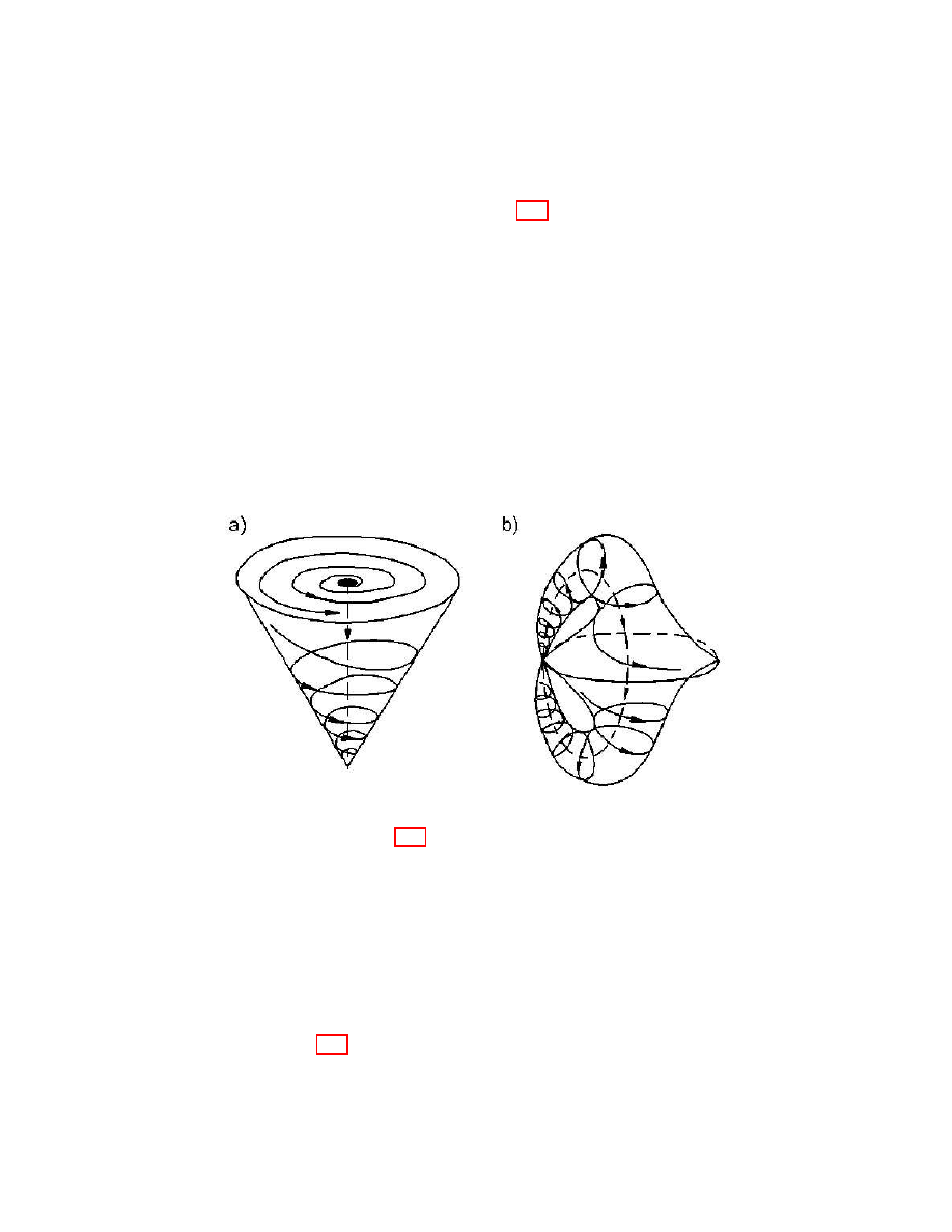
Figure 1.
ω(x, k)-, but not Ω(x, k)-bifurcations: a - phase por-
trait of the system (1.14); b - the same portrait after gluing all
fixed points.
Example 1.16. (ω(x, k)-, but not Ω(x, k)-bifurcations). Consider at first the sys-
tem, given in the cone x
2
+ y
2
≤ z
2
, 0 ≤ z ≤ 1 by differential equations (in
cylindrical coordinates)
˙r = r(2z − r − 1)
2
− 2r(1 − r)(1 − z);
˙
ϕ = r cos ϕ + 1;
˙
z = −z(1 − z)
2
.
(1.14)
The solutions of (1.14) under initial conditions 0 ≤ z(0) ≤ 1, 0 ≤ r(0) ≤ z(0) and
arbitrary ϕ tend to their unique ω-limit point as t → ∞ (this point is the equilibrium
z = r = 0). If 0 < r(0) < 1, then the solution tends to the circumference z = r = 1

EJDE-2004/MON. 05
SINGULARITIES OF TRANSITION PROCESSES
19
as t → ∞. If z(0) = 1, r(0) = 0, then the ω-limit point is unique: z = 1, r = 0. If
z(0) = r(0) = 1, then the ω-limit point is also unique: z = r = 1, ϕ = π (Fig. 1).
Thus,
ω(r
0
, ϕ
0
, z
0
) =
(z = r = 0),
if z
0
< 1;
{(r, ϕ, z) : r = z = 1},
if z
0
= 1, r
0
6= 0, 1;
(z = r = 1), ϕ = π,
if z
0
= r
0
= 1;
(r = 0, z = 1),
if z
0
= 1, r
0
= 0 .
Consider the sequence of points of the cone (r
n
, ϕ
n
, z
n
) → (r
∗
, ϕ
∗
, 1), r
∗
6= 0, 1 and
z
n
< 1 for all n. For any point of the sequence the ω-limit set includes one point, and
for (r
∗
, ϕ, 1) the set includes the circumference. If all the positions of equilibrium
were identified, then there would be ω(x, k)-, but not ω(x, k)-bifurcations.
The correctness of the identification procedure should be guaranteed. Let the
studied semiflow f have fixed points x
i
, . . . , x
n
. Define a new semiflow ˜
f as follows:
˜
X = X \ {x
i
, . . . , x
n
} ∪ {x
∗
}
is a space obtained from X when the points x
i
, . . . , x
n
are deleted and a new point
x
∗
is added. Let us give metrics over ˜
X as follows: Let x, y ∈ ˜
X, x 6= x
∗
,
˜
ρ(x, y) =
(
min{ρ(x, y), min
1≤j≤n
ρ(x, x
j
) + min
1≤j≤n
ρ(y, x
j
)},
if y 6= x
∗
;
min
1≤j≤n
ρ(x, x
j
),
if y = x
∗
.
Let ˜
f (t, x) = f (t, x) if x ∈ X
T
˜
X, ˜
f (t, x
∗
) = x
∗
.
Lemma 1.17. The mapping ˜
f determines a semiflow in ˜
X.
Proof. Injectivity and semigroup property are obvious from the corresponding prop-
erties of f . If x ∈ X
T
˜
X, t ≥ 0 then the continuity of ˜
f in the point (t, x) follows
from the fact that ˜
f coincides with f in some neighbourhood of this point. The
continuity of ˜
f in the point (t, x
∗
) follows from the continuity of f and the fact that
any sequence converging in ˜
X to x
∗
can be divided into finite number of sequences,
each of them being either (a) a sequence of points X
T
˜
X, converging to one of x
j
or (b) a constant sequence, all elements of which are x
∗
and some more, maybe, a
finite set. Mapping ˜
f is a homeomorphism, since it is continuous and injective, and
˜
X is compact.
Proposition 1.18. Let each trajectory lying in ω(k) be recurrent for any k. Then
the existence of ω(x, k)- (ω(k)-)-bifurcations is equivalent to the existence of Ω(x, k)-
(Ω(k)-)-bifurcations. More precisely:
(A) if (x
n
, k
n
) → (x
∗
, k
∗
) and ω(x
n
, k
n
) 6→ ω(x
∗
, k
∗
), then Ω(x
n
, k
n
) 6→ Ω(x
∗
, k
∗
).
(B) if k
n
→ k
∗
and ω(k
n
) 6→ ω(k
∗
), then Ω(k
n
) 6→ Ω(k
∗
).
(Let us recall that the convergence in B(X) implies d-convergence, and the conver-
gence in B(B(X)) implies D-convergence, and continuity is considered as continuity
with respect to these convergence, if there are no other mentions.)
Proof. (A) Let (x
n
, k
n
) → (x
∗
, k
∗
), ω(x
n
, k
n
) 6→ ω(x
∗
, k
∗
). Then, according to
Proposition 1.9, there exists ˜
x ∈ (x
∗
, k
∗
) such that inf
y∈ω(x
n
,k
n
)
ρ(˜
x, y) 6→ 0. There-
fore, from {(x
n
, k
n
)} we can choose a subsequence (denoted as {(x
m
, k
m
)}) for
which there exists such ε > 0 that inf
y∈ω(x
m
,k
m
)
ρ(˜
x, y) > ε for any m = 1, 2 < . . . .
Denote by L the set of all limit points of sequences of the kind {y
m
}, y
m
∈

20
A. N. GORBAN
EJDE-2004/MON. 05
ω(x
m
, k
m
). The set L is closed and k
∗
-invariant. Note that ρ
∗
(˜
x, L) ≥ ε. There-
fore, ω(˜
x, k
∗
)
T L = ∅ as ω(˜x, k
∗
) is a minimal set (Birkhoff’s theorem, see [56,
p.404]). From this follows the existence of such δ > 0 that r(ω(˜
x, k
∗
), L) > δ and
from some M r(ω(˜
x, k
∗
), (x
m
, k
m
)) > δ/2 (when m > M ). Therefore, (Proposition
1.12) Ω(x
m
, k
m
) 6→ Ω(x
∗
, k
∗
).
(B) The proof practically coincides with that for the part A (it should be substituted
ω(k) for ω(x, k)).
Corollary 1.19. For every pair (x, k) ∈ X × K let the ω-limit set be minimal:
Ω(x, k) = {ω(x, k)}. Then statements A, B of Proposition 1.18 hold.
Proof. According to one of Birkhoff’s theorems [56, p.402], each trajectory lying in
minimal set is recurrent. Therefore, Proposition 1.18 is applicable.
2. Slow Relaxations
2.1. Relaxation Times. The principal object of our consideration is the relaxation
time. The system of the relaxation times is defined in Introduction.
Proposition 2.1. For any x ∈ X, k ∈ K and ε > 0 the numbers τ
i
(x, k, ε) and
η
i
(x, k, ε) (i = 1, 2, 3) are defined, and the inequalities τ
i
≥ η
i
, τ
1
≤ τ
2
≤ τ
3
,
η
1
≤ η
2
≤ η
3
hold.
Proof. If τ
i
, η
i
are defined, then the validity of inequalities is obvious (ω(x, k) ⊂
ω(k), the time of the first entry in the ε-neighbourhood of the set of limit points is
included into the time of being outside of this neighbourhood, and the last is not
larger than the time of final entry in it). The numbers τ
i
, η
i
are definite (bounded):
there are t
n
∈ [0, ∞), t
n
→ ∞ and y ∈ ω(x, k), for which f (t
n
, x, k) → y and from
some n, ρ(f (t
n
, x, k), y) < ε; therefore ,the sets {t > 0 : ρ
∗
(f (t, x, k), ω(x, k)) < ε}
and {t > 0 : ρ
∗
(f (t, x, k), ω(k)) < ε} are nonempty. Since X is compact, there is
such t(ε) > 0 that for t > t(ε) ρ
∗
(f (t, x, k), ω(x, k)) < ε. In fact, let us suppose
the contrary: there are such t
n
> 0 that t
n
→ ∞ and ρ
∗
(f (t
n
, x, k), ω(x, k)) > ε.
Let us choose from the sequence f (t
n
, x, k) a convergent subsequence and denote
its limit x
∗
; x
∗
satisfies the definition of ω-limit point of (k, x)-motion, but it lies
outside of ω(x, k). The obtained contradiction proves the required, consequently,
τ
3
and η
3
are defined. According to the proved, the sets
{t > 0 : ρ
∗
(f (t, x, k), ω(x, k)) ≥ ε},
{t > 0 : ρ
∗
(f (t, x, k), ω(k)) ≥ ε}
are bounded. They are measurable because of the continuity with respect to t
of the functions ρ
∗
(f (t, x, k), ω(x, k)) and ρ
∗
(f (t, x, k), ω(k)). The proposition is
proved.
Note that the existence (finiteness) of τ
2,3
and η
2,3
is associated with the com-
pactness of X.
Definition 2.2. We say that the system (1.1) possesses τ
i
- (η
i
-)-slow relaxations,
if for some ε > 0 the function τ
i
(x, k, ε) (respectively η
i
(x, k, ε)) is not bounded
above in X × K.
Proposition 2.3. For any semiflow (k is fixed) the function η
1
(x, ε) is bounded in
X for every ε > 0.
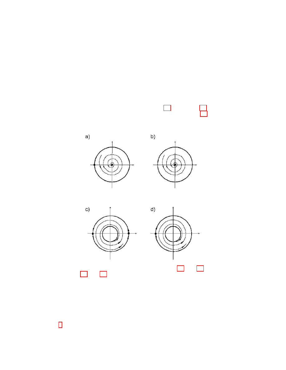
EJDE-2004/MON. 05
SINGULARITIES OF TRANSITION PROCESSES
21
Proof. Suppose the contrary.
Then there is such sequence of points x
n
∈ X
that for some ε > 0 η
1
(x
n
, ε) → ∞. Using the compactness of X and, if it is
needed, choosing a subsequence, assume that x
n
→ x
∗
. Let us show that for any
t > 0 ρ
∗
(f (t, x
∗
), ω(k)) > ε/2.
Because of the property of uniform continuity
on bounded segments there is such δ = δ(τ ) > 0 that ρ(f (t, x
∗
), f (t, x)) < ε/2
if 0 ≤ t ≤ τ and ρ(x, x
∗
) < δ. Since η
1
(x
n
, ε) → ∞ and x
n
→ x
∗
, there is
such N that ρ(x
N
, x
∗
) < δ and η
1
(x
N
, ε) > τ , i.e. ρ
∗
(f (t, x
N
), ω(k)) ≥ ε under
0 ≤ t ≤ τ . From this we obtain the required: for 0 ≤ t ≤ τ ρ
∗
(f (t, x
∗
), ω(k)) > ε/2
or ρ
∗
(f (t, x
∗
), ω(k)) > ε/2 for any t > 0, since τ was chosen arbitrarily. This con-
tradicts to the finiteness of η
1
(x
∗
, ε/2) (Proposition 2.1). Proposition 2.3 is proved.
For η
2,3
and τ
1,2,3
does not exist proposition analogous to Proposition 2.3, and slow
relaxations are possible for one semiflow too.
Figure 2.
Phase portraits of the systems: a - (2.1); b - (2.2); c
Example 2.4 (η
2
-slow relaxations for one semiflow). Consider a system on the
plane in the circle x
2
+ y
2
≤ 1 given by the equations in the polar coordinates
˙r = −r(1 − r)(r cos ϕ + 1);
˙
ϕ = r cos ϕ + 1.
(2.1)
The complete ω-limit set consists of two fixed points r = 0 and r = 1, ϕ = π (Fig.
2,a), η
2
((r, ϕ), 1/2) → ∞ as r → 1, r < 1.

22
A. N. GORBAN
EJDE-2004/MON. 05
The following series of simple examples is given to demonstrate the existence of
slow relaxations of some kinds without some other kinds.
Example 2.5 (η
3
- but not η
2
-slow relaxations). Let us modify the previous exam-
ple, substituting unstable limit cycle for the boundary loop:
˙r = −r(1 − r);
˙
ϕ = 1.
(2.2)
Now the complete ω-limit set includes the whole boundary circumference and the
point r = 0 (Fig. 2,b), the time of the system being outside of its ε-neighborhood
is bounded for any ε > 0. Nevertheless, η
3
((r, ϕ), 1/2) → ∞ as r → 1, r 6= 1
Example 2.6 (τ
1
, but not η
2,3
-slow relaxations). Let us analyze in the ring
1
2
≤
x
2
+ y
2
≤ 1 a system given by differential equations in polar coordinates
˙r = (1 − r)(r cos ϕ + 1)(1 − r cos ϕ);
˙
ϕ = (r cos ϕ + 1)(1 − r cos ϕ).
In this case the complete ω-limit set is the whole boundary circumference r = 1
(Fig. 2,c). Under r = 1, ϕ → π, ϕ > π τ
1
(r, ϕ, 1/2) → ∞ since for these points
ω(r, ϕ) = {(r = 1, ϕ = 0)}.
Example 2.7 (τ
3
, but not τ
1,2
and not η
3
-slow relaxations). Let us modify the
preceding example of the system in the ring, leaving only one equilibrium point on
the boundary circumference r = 1:
˙r = (1 − r)(r cos ϕ + 1);
˙
ϕ = r cos ϕ + 1.
(2.3)
In this case under r = 1, ϕ → π, ϕ → π τ
3
((r, ϕ), 1/2) → ∞ and τ
1,2
remain
bounded for any fixed ε > 0, because for these points ω(r, ϕ) = {(r = 1, ϕ = π)}
(Fig. 2,d). η
2,3
are bounded, since the complete ω-limit set is the circumference
r = 1.
Example 2.8 (τ
2
, but not τ
1
and not η
2
-slow relaxations). We could not find a
simple example on the plane without using Lemma 1.17. Consider at first a semiflow
in the circle x
2
+ y
2
≤ 2 given by the equations
˙r = −r(1 − r)
2
[(r cos ϕ + 1)
2
+ r
2
sin ϕ];
˙
ϕ = (r cos ϕ + 1)
2
+ r
2
sin
2
ϕ.
the ω-limit sets of this system are as follows (Fig. 3,a):
ω(r
0
, ϕ
0
) =
circumference r = 1,
if r
0
> 1;
point (r = 1, ϕ = π),
if r
0
= 1;
point (r = 0),
if r
0
< 1.
Let us identify the fixed points (r = 1, ϕ = π) and (r = 0) (Fig. 3,b). We obtain
that under r → 1, r < 1 τ
2
(r, ϕ, 1/2) → ∞, although τ
1
remains bounded as well
as η
2
. However, η
3
is unbounded.
The majority of the above examples is represented by non-rough systems, and
there are serious reasons for this non-roughness. In rough systems on a plane τ
1,2,3
-
and η
3
-slow relaxations can occur only simultaneously (see Subsection 3.3).
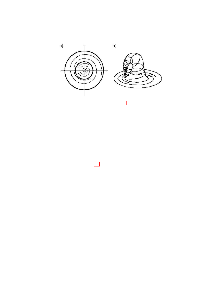
EJDE-2004/MON. 05
SINGULARITIES OF TRANSITION PROCESSES
23
Figure 3.
Phase portrait of the system (2.4):
a - without gluing the fixed points; b - after gluing.
2.2. Slow Relaxations and Bifurcations of ω-limit Sets. In the simplest sit-
uations the connection between slow relaxations and bifurcations of ω-limit sets
is obvious. We should mention the case when the motion tending to its ω-limit
set is retarded near unstable equilibrium position. In general case the situation
becomes more complicated at least because there are several relaxation times (and
consequently several corresponding kinds of slow relaxations). Except that, as it
will be shown below, bifurcations are not a single possible reason of slow relaxation
appearance. Nevertheless, for the time of the first entering (both for the proper
time τ
1
and for the non-proper one η
1
) the connection between bifurcations and
slow relaxations is manifest.
Theorem 2.9. The system (1.1) possesses τ
1
-slow relaxations if and only if it
possesses Ω(x, k)-bifurcations.
Proof. Let the system possess Ω(x, k)-bifurcations, (x
∗
, k
∗
) be the point of bifur-
cation. This means that there are such x
0
∈ X, ε > 0 and sequence of points
(x
n
, k
n
) ∈ X × K, for which ω(x
0
, k
∗
) ⊂ ω(x
∗
, k
∗
), (x
n
, k
n
) → (x
∗
, k
∗
), and
r(ω(x
0
, k
∗
), ω(x
n
, k
n
)) > ε for any n. Let x
0
∈ ω(x
0
, k
∗
). Then ω(x
0
, k
∗
) ⊂ ω(x
0
, k
∗
)
and r(ω(x
0
, k
∗
), ω(x
n
, k
n
)) > ε for any n. Since x
0
∈ ω(x
∗
, k
∗
), there is such se-
quence t
i
> 0, t → ∞, for which f (t
i
, x
∗
, k
∗
) → x
0
. As for every i f (t
i
, x
n
, k
n
) →
f (t
i
, x
∗
, k
∗
), then there is such sequence n(i) that f (t
i
, x
n(i)
, k
n(i)
) → x
0
as i →
∞. Denote k
n(i)
as k
0
i
and f (t
i
, x
n(i)
, k
n(i)
) as y
i
. It is obvious that ω(y, k
0
i
) =
ω(x
n(i)
, k
n(i)
). Therefore r(ω(x
0
, k
∗
), ω(y
i
, k
0
i
)) > ε.
Let us show that for any τ > 0 there is i such that τ
1
(y
i
, k
0
i
, ε/2) > τ . To do that,
use the uniform continuity of f on compact segments and choose δ > 0 such that
ρ(f (t, x
0
, k
∗
), f (t, y
i
, k
0
i
)) < ε/2 if 0 ≤ t ≤ τ, ρ(x
0
, y
i
) + ρ
K
(k
∗
, k
0
i
) < δ. The last
inequality is true for some i
0
(when i > i
0
), since y
i
→ x
0
and k
0
i
→ k
∗
. For any
t ∈ (−∞, ∞), f (t, x
0
, k
∗
) ∈ ω(x
0
, k
∗
), consequently, ρ
∗
(f (t, y
i
, k
0
i
), ω(y
i
, k
0
i
)) > ε/2
for i > i
0
, 0 ≤ t ≤ τ ; therefore, for these i τ
1
(y
i
, k
0
i
, ε/2) > τ . The existence of
τ
1
-slow relaxations is proved.
Now, let us suppose that there are τ
1
-slow relaxations: There can be found a
sequence (x
n
, k
n
) ∈ X × K such that for some ε > 0, τ
1
(x
n
, k
n
, ε) → ∞. Using

24
A. N. GORBAN
EJDE-2004/MON. 05
the compactness of X × K, choose from this sequence a convergent one, preserving
the denotations: (x
n
, k
n
) → (x
∗
, k
∗
). For any y ∈ ω(x
∗
, k
∗
) there is n = n(y) such
that when n > n(y) ρ
∗
(y, ω(x
n
, k
n
)) > ε/2. In deed as y ∈ ω(x
∗
, k
∗
), there is t > 0
such that ρ(f (t, x
∗
, k
∗
), y) < ε/4. Since (x
n
, k
n
) → (x
∗
, k
∗
), τ
1
(x
n
, k
n
, ε) → ∞,
there is n (we denote it by n(y)) such that for n > n(y) ρ
∗
(¯
t, x
n
, k
n
)) < ε/4,
τ
1
(x
n
, k
n
, ε) > t. Therefore, since ρ
∗
(f (¯
t, x
n
, k
n
), ω(x
n
, k
n
)) > ε, it follows that
ρ
∗
(f (¯
t, x
∗
, k
∗
), ω(x
n
, k
n
)) > 3ε/4, and, consequently, ρ
∗
(y, ω(x
n
, k
n
)) > ε/2. Let
y
i
, . . . , y
m
be ε/4-network in ω(x
∗
, k
∗
). Let N = max n(y
i
). Then for n > N and
for any i (1 ≤ i ≤ m), ρ
∗
(y
i
, ω(x
n
, k
n
)) > ε/2. Consequently, for any y ∈ ω(x
∗
, k
∗
)
for n > N ρ
∗
(y, ω(x
n
, k
n
) > ε/4, i.e. for n > N r(ω(x
∗
, k
∗
), ω(x
n
, k
n
)) > ε/4. The
existence of Ω(x, k)-bifurcations is proved (according to Proposition 1.12). Using
Theorem 2.9 and Proposition 1.15 we obtain the following theorem.
Theorem 2.9
The system (1.1) possesses τ
1
-slow relaxations if and only if ω(x, k)
is not r-continuous function in X × K.
Theorem 2.10. The system (1.1) possesses η
1
-slow relaxations if and only if it
possesses Ω(k)-bifurcations.
Proof. Let the system possess Ω(k)-bifurcations. Then (according to Proposition
1.12) there is such sequence of parameters k
n
→ k
∗
that for some ω(x
∗
, k
∗
) ∈ Ω(k
∗
)
and ε > 0 for any n r(ω(x
∗
, k
∗
), ω(k
n
)) > ε. Let x
0
∈ ω(x
∗
, k
∗
). Then for any
n and t ∈ (−∞, ∞) ρ
∗
(f (t, x
0
, k
∗
), ω(k
n
)) > ε because f (t, x
0
, k
∗
) ∈ ω(x
∗
, k
∗
).
Let us prove that η
1
(x
0
, k
n
, ε/2) → ∞ as n → ∞. To do this, use the uniform
continuity of f on compact segments and for any τ > 0 find such δ = δ(τ ) > 0 that
ρ(f (t, x
0
, k
∗
), f (t, x
0
, k
n
)) < ε/2 if 0 ≤ t ≤ τ and ρ
K
(k
∗
, k
n
) < δ. Since k
n
→ k
∗
,
there is such N = N (τ ) that for n > N ρ
K
(k
n
, k) < δ. Therefore, for n > N ,
0 ≤ t ≤ τ ρ
∗
(f (t, x
0
, k
n
), ω(k
n
)) > ε/2. The existence of η
1
-slow relaxations is
proved.
Now, suppose that there exist η
1
-slow relaxations: there are such ε > 0 and
sequence (x
n
, k
n
) ∈ X × K that η
1
(x
n
, k
n
, ε) → ∞.
Use the compactness of
X × K and turn to converging subsequence (retaining the same denotations):
(x
n
, k
n
) → (x
∗
, k
∗
). Using the way similar to the proof of Theorem 2.9, let us
show that for any y ∈ ω(x
∗
, k
∗
) there is such n = n(y) that if n > n(y), then
ρ
∗
(y, ω(k
n
)) > ε/2.
Really, there is such ˜
t > 0 that ρ(f (˜
t, x
∗
, k
∗
), y) < ε/4.
As η
1
(x
n
, k
n
, ε) → ∞ and (x
n
, k
n
) → (x
∗
, k
∗
), there is such n = n(y) that for
n > n(y) ρ(f (˜
t, x
∗
, k
∗
), f (˜
t, x
n
, k
n
)) < ε/4 and η
1
(x
n
, k
n
, ε) > ˜
t. Thereafter we
obtain
ρ
∗
(y, ω(k
n
))
≥ ρ
∗
(f (t, x
n
, k
n
), ω(k
n
)) − ρ(y, f (˜
t, x
∗
, k
∗
)) − ρ(f (˜
t, x
∗
, k
∗
), f (˜
t, x
n
, k
n
)) > ε/2.
Further the reasonings about ε/4-network of the set ω(x
∗
, k
∗
) (as in the proof of
Theorem 2.9) lead to the inequality r(ω(x
∗
, k
∗
), ω(k
n
)) > ε/4 for n large enough.
On account of Proposition 1.12 the existence of Ω(k)-bifurcations is proved, there-
fore is proved Theorem 2.10.
Theorem 2.11. If the system (1.1) possesses ω(x, k)-bifurcations then it possesses
τ
2
-slow relaxations.

EJDE-2004/MON. 05
SINGULARITIES OF TRANSITION PROCESSES
25
Proof. Let the system (1.1) possess ω(x, k)-bifurcations: there is a sequence (x
n
, k
n
) ∈
X × K and ε > 0 such that (x
n
, k
n
) → (x
∗
, k
∗
) and
ρ
∗
(x
0
, ω(x
n
, k
n
)) > ε for any n and some x
0
∈ ω(x
∗
, k
∗
).
Let t > 0. Define the following auxiliary function:
Θ(x
∗
, x
0
, t, ε) = meas{t
0
≥ 0 : t
0
≤ t, ρ(f (t
0
, x
∗
, k
∗
), x
0
) < ε/4},
(2.4)
Θ(x
∗
, x
0
, t, ε) is “the time of residence” of (k
∗
, x
∗
)-motion in ε/4-neighbourhood of
x over the time segment [0, t]. Let us prove that Θ(x
∗
, x
0
, t, ε) → ∞ as t → ∞. We
need the following corollary of continuity of f and compactness of X
Lemma 2.12. Let x
0
∈ X, k ∈ K, δ > ε > 0. Then there is such t
0
> 0 that for
any x ∈ X the inequalities ρ(x, x
0
) < ε and 0 ≤ t
0
< t
0
lead to ρ(x
0
, f (t
0
, x, k)) < δ.
Proof. Let us suppose the contrary: there are such sequences x
n
and t
n
that
ρ(x
0
, x
n
) < ε, t
0
n
→ 0, and ρ(x
0
, f (t
0
n
, x
n
, k)) ≥ δ. Due to the compactness of
X one can choose from the sequence x
n
a convergent one.
Let it converge to
¯
x. The function ρ(x
0
, f (t, x, k)) is continuous. Therefore, ρ(x
0
, f (t
0
n
, x
n
, k)) →
ρ(x
0
, f (0, x, k)) = ρ(x
0
, ¯
x). Since ρ(x
0
, x
n
) < ε, then ρ(x
0
, ¯
x) ≤ ε. This contradicts
to the initial supposition (ρ(x
0
, f (t
0
n
, x
n
, k)) ≥ δ ≥ ε).
Let us return to the proof of Theorem 2.11. Since x
0
∈ ω(x
∗
, k
∗
), then there
is such monotonic sequence t
j
→ ∞ that for any j ρ(f (t
j
, x
∗
, k
∗
), x
0
) < ε/8. Ac-
cording to Lemma 2.12 there is t
0
> 0 for which ρ(f (t
j
+ τ, x
∗
, k
∗
), x
0
) < ε/4 as
0 ≤ τ ≤ t
0
. Suppose (turning to subsequence, if it is necessary) that t
j+1
− t
j
> t
0
.
Θ(x
∗
, x
0
, t, ε) > jt
0
if t > t
j
+ t
0
. For any j = 1, 2, . . . there is such N (j) that
ρ(f (t, x
n
, k
n
), f (t, x
∗
, k
∗
)) < ε/4 under the conditions n > N (j), 0 ≤ t ≤ t
j
+ t
0
.
If n > N (j), then ρ(f (t, x
n
, k
n
), x
0
) < ε/2 for t
j
≤ t ≤ t
j
+ t
0
(i ≤ j). Conse-
quently, τ
2
(x
n
, k
n
, ε/2) > jt
0
if n > N (j). The existence of τ
2
slow relaxations is
proved.
Theorem 2.13. If the system (1.1) possesses ω(k)-bifurcations, then it possesses
η
2
-slow relaxations too.
Proof. Let the system (1.1) possess ω(k)-bifurcations: there are such sequence k
n
∈
K and such ε > 0 that k
n
> k
∗
and ρ
∗
(x
0
, ω(k
n
)) > ε for some x
0
∈ ω(k
∗
) and
any n. The point x
0
belongs to the ω-limit set of some motion: x
0
∈ ω(x
∗
, k
∗
). Let
τ > 0 and t
∗
be such that Θ(x
∗
, x
0
, t
∗
, ε) > τ (the existence of such t
∗
is shown when
proving Theorem 2.11). Due to the uniform continuity of f on compact intervals
there is such N that ρ(f (x
∗
, k
∗
), f (t, x
∗
, k
n
)) < ε/4 for 0 ≤ t ≤ t
∗
, n > N . But
from this fact it follows that η
2
(x
∗
, k
n
, ε/2) ≥ Θ(x
∗
, x
0
, t
∗
, ε) > τ (n > N ). Because
of the arbitrary choice of τ Theorem 2.13 is proved.
The two following theorems provide supplementary sufficient conditions of τ
2
-
and η
2
-slow relaxations.
Theorem 2.14. If for the system (1.1) there are such x ∈ X, k ∈ K that (k, x)-
motion is whole and α(x, k) 6⊂ ω(x, k), then the system (1.1) possesses τ
2
-slow
relaxations.
Proof. Let there be such x and k that (k, x)-motion is whole and α(x, k) 6⊂ ω(x, k).
Let us denote by x
∗
an arbitrary α-, but not ω-limit point of (k, x)-motion. Since
ω(x, k) is closed, ρ
∗
(x
∗
, ω(x, k)) > ε > 0. Define an auxiliary function
ϕ(x, x
∗
, t, ε) = meas{t
0
: −t ≤ t
0
≤ 0, ρ(f (t
0
, x, k), x
∗
) < ε/2}.
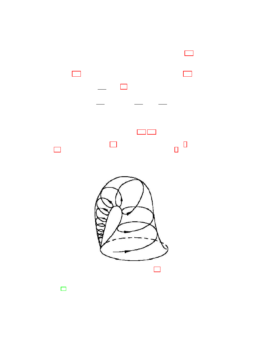
26
A. N. GORBAN
EJDE-2004/MON. 05
Let us prove that ϕ(x, x
∗
, ε) → ∞ as t → ∞. According to Lemma 2.12 there is
such t
0
> 0 that ρ(f (t, y, k), x
∗
) < ε/2 if 0 ≤ t ≤ t
0
and ρ(x
∗
, y) < ε/4. Since x
∗
is α-limit point of (k, x)-motion, there is such sequence t
j
< 0, t
j+1
− t
j
< −t
0
,
for which ρ(f (t
j
, x, k), x
∗
) < ε/4.
Therefore, by the way used in the proof of
Theorem 2.11 we obtain: ϕ(x, x
∗
, t
j
, ε) > jt
0
. This proves Theorem 2.14, because
τ
2
(f (−t, x, k), k, ε/2) ≥ ϕ(x, x
∗
, t, ε).
Theorem 2.15. If for the system (1.1) exist such x ∈ X, k ∈ K that (k, x)-motion
is whole and α(x, k) 6⊂ ω(k), then the system (1.1) possesses η
2
-slow relaxations.
Proof. Let (k, x)-motion be whole and
α(x, k) 6⊂ ω(k), x
∗
∈ α(x, k) \ ω(k), ρ
∗
(x
∗
, ω(k)) = ε > 0.
As in the proof of the previous theorem, let us define the function ϕ(x, x
∗
, t, ε).
Since ϕ(x, x
∗
, t, ε) → ∞ as t → ∞ (proved above) and η
2
(f (−t, x, k), k, ε/2) ≥
ϕ(x, x
∗
, t, ε), the theorem is proved.
Note that the conditions of the theorems 2.14, 2.15 do not imply bifurcations.
Example 2.16 (τ
2
-, η
2
-slow relaxations without bifurcations). Examine the system
given by the set of equations (2.1) in the circle x
2
+ y
2
≤ 1 (see Fig. 2,a, Example
2.4). Identify the fixed points r = 0 and r = 1, ϕ = π (Fig. 4). The complete
ω-limit set of the system obtained consists of one fixed point.
For initial data
r
0
→ 1, r
0
< 1 (ϕ
0
is arbitrary) the relaxation time η
2
(r
0
, ϕ
0
, 1/2) → ∞ (hence,
τ
2
(r
0
, ϕ
0
, 1/2) → ∞).
Figure 4.
Phase portrait of the system (2.1) after gluing the
fixed points.
Before analyzing τ
3
, η
3
-slow relaxations, let us define Poisson’s stability according
to [56], p.363: (k, x)-motion is it Poisson’s positively stable (P
+
-stable), if x ∈
ω(x, k).
Note that any P
+
-stable motion is whole.

EJDE-2004/MON. 05
SINGULARITIES OF TRANSITION PROCESSES
27
Lemma 2.17. If for the system (1.1) exist such x ∈ X, k ∈ K that (k, x)-motion
is whole but not P
+
-stable, then the system (1.1) possesses τ
3
-slow relaxations.
Proof. Let ρ
∗
(x, ω(x, k)) = ε > 0 and (k, x)-motion be whole. Then
τ
3
(f (−t, x, k), k, ε) ≥ t, since f (t, f (−t, x, k), k) = x and ρ
∗
(x, ω(f (−t, x, k), k)) = ε
(because ω(f (−t, x, k), k) = ω(x, k)). Therefore, τ
3
-slow relaxations exist.
Lemma 2.18. If for the system (1.1) exist such x ∈ X, k ∈ K that (k, x)-motion
is whole and x 6∈ ω(k), then this system possesses η
3
-slow relaxations.
Proof. Let ρ
∗
(x, ω(k)) = ε > 0 and (k, x)-motion be whole. Then
η
3
(f (−t, x, k), k, ε)) ≥ t,
since f (t, f (−t, x, k), k) = x and ρ
∗
(x, ω(k)) = ρ
∗
(x, ω(k)) = ε.
Consequently, η
3
-slow relaxations exist.
Lemma 2.19. Let for the system (1.1) be such x
0
∈ X, k ∈ K that (k
0
, x
0
)-
motion is whole. If ω(x, k) is d-continuous function in X × K (there are no ω(x, k)-
bifurcations), then:
(1) ω(x
∗
, k
0
) ⊂ ω(x
0
, k
0
) for any x
∗
∈ α(x
0
, k
0
), that is ω(α(x
0
, k
0
), k
0
) ⊂
ω(x
0
, k
0
);
(2) In particular, ω(x
0
, k
0
)
T α(x
0
, k
0
) 6= ∅.
Proof. Let x
∗
∈ α(x
0
, k
0
). Then there are such t
n
> 0 that t
n
→ ∞ and x
n
=
f (−t
n
, x
0
, k
0
) → x
∗
. Note that ω(x
n
, k
0
) = ω(x
0
, k
0
). If ω(x
∗
, k
0
) 6⊂ ω(x
0
, k
0
),
then, taking into account closure of ω(x
0
, k
0
), we obtain d(ω(x
∗
, k
0
), ω(x
0
, k
0
)) >
0. In this case x
n
→ x
∗
, but ω(x
n
, k
0
) − / → ω(x
∗
, k
0
), i.e. there is ω(x, k)-
bifurcation. But according to the assumption there are no ω(x, k)-bifurcations.
The obtained contradiction proves the first statement of the lemma. The second
statement follows from the facts that α(x
0
, k
0
) is closed, k
0
-invariant and nonempty.
Really, let x
∗
∈ α(x
0
, k
0
). Then f ((−∞, ∞), x
∗
, k
o
) ⊂ α(x
0
, k
0
) and, in particular,
ω(x
∗
, k
0
) ⊂ α(x
0
, k
0
). But it has been proved that ω(x
∗
, k
0
) ⊂ ω(x
0
, k
0
). Therefore,
ω(x
0
, k
0
)
T α(x
0
, k
0
) ⊃ ω(x
∗
, k
0
) 6= ∅.
Theorem 2.20. The system (1.1) possesses τ
3
-slow relaxations if and only if at
least one of the following conditions is satisfied:
(1) There are ω(x, k)-bifurcations;
(2) There are such x ∈ X, k ∈ K that (k, x)-motion is whole but not P
+
-stable.
Proof. If there exist ω(x, k)-bifurcations, then the existence of τ
3
-slow relaxations
follows from Theorem 2.11 and the inequality τ
2
(x, k, ε) ≤ τ
3
(x, k, ε). If the con-
dition 2 is satisfied, then the existence of τ
3
-slow relaxations follows from Lemma
2.17. To finish the proof, it must be ascertained that if the system (1.1) pos-
sesses τ
3
-slow relaxations and does not possess ω(x, k)-bifurcations, then there
exist such x ∈ X, k ∈ K that (k, x)-motion is whole and not P
+
-stable. Let
there be τ
3
-slow relaxations and ω(x, k)-bifurcations be absent. There can be cho-
sen such convergent (because of the compactness of X × K) sequence (x
n
, k
n
) →
(x
∗
, k
∗
) that τ
3
(x
n
, k
n
, ε) → ∞ for some ε > 0.
Consider the sequence y
n
=
f (τ
3
(x
n
, k
n
, ε), x
n
, k
n
). Note that ρ
∗
(y
n
, ω(x
n
, k
n
)) = ε. This follows from the def-
inition of relaxation time and continuity of the function ρ
∗
(f (t, x, k), s) of t at any
(x, k) ∈ X × K, s ⊂ X. Let us choose from the sequence y
n
a convergent one
28
A. N. GORBAN
EJDE-2004/MON. 05
(preserving the denotations y
n
, x
n
, k
n
). Let us denote its limit: y
n
→ x
0
. It is clear
that (k
∗
, x
0
)-motion is whole. This follows from the results of Subection 1.1 and
the fact that (k
n
, y
n
)-motion is defined in the time interval [−τ
3
(x
n
, k
n
, ε), ∞), and
τ
3
(x
n
, k
n
, ε) → ∞ as n → ∞. Let us prove that (k
∗
, x
0
)-motion is not P
+
-stable, i.e.
x
0
6∈ ω(x
0
, k
∗
). Suppose the contrary: x
0
∈ ω(x
0
, k
∗
). Since y
n
→ x
0
, then there is
such N that ρ(x
0
, y
n
) < ε/2 for any n ≥ N . For the same n ≥ N ρ
∗
(x
0
, ω(y
n
, k
n
)) >
ε/2, since ρ
∗
(y
n
, ω(y
n
, k
n
)) = ε.
But from this fact and from the assumption
x
0
∈ ω(x
0
, k
∗
) it follows that for n ≥ N d(ω(x
0
, k
∗
), ω(y
n
, k
n
)) > ε/2, and that
means that there are ω(x, k)-bifurcations. So far as it was supposed d-continuity
of ω(x, k), it was proved that (k
∗
, x
0
)-motion is not P
+
-stable, and this completes
the proof of the theorem.
Using Lemma 2.19, Theorem 2.20 can be formulated as follows.
Theorem 2.20
. The system (1.1) possesses τ
3
-slow relaxations if and only if at
least one of the following conditions is satisfied:
(1) There are ω(x, k)-bifurcations;
(2) There are such x ∈ X, k ∈ K that (k, x)-motion is whole but not P
+
-stable
and possesses the following property: ω(α(x, k), k) ⊂ ω(x, k).
As an example of motion satisfying the condition 2 can be considered a trajectory
going from a fixed point to the same point (for example, the loop of a separatrice),
or a homoclinical trajectory of a periodical motion.
Theorem 2.21. The system (1.1) possesses η
3
-slow relaxations if and only if at
least one of the following conditions is satisfied:
(1) There are ω(k)-bifurcations;
(2) There are such x ∈ X, k ∈ K that (k, x)-motion is whole and x 6∈ ω(k).
Proof. If there are ω(k)-bifurcations, then, according to Theorem 2.13, there are
η
2
- and all the more η
3
-slow relaxations. If the condition 2 holds, then the existence
of η
3
-slow relaxations follows from Lemma 2.18. To complete the proof, it must
be established that if the system (1.1) possesses η
3
-slow relaxations and does not
possess ω(k)-bifurcations then the condition 2 of the theorem holds: there are such
x ∈ X, k ∈ K (k, x)-motion is whole and x 6∈ ω(k). Let there be η
3
-slow relaxation
and ω(k)-bifurcations be absent. Then we can choose such convergent (because of
the compactness of X × K) sequence (x
n
, k
n
) → (x
∗
, k
∗
) that η
3
(x
n
, k
n
, ε) → ∞
for some ε > 0. Consider the sequence y
n
= f (η
3
(x
n
, k
n
, ε), x
n
, k
n
). Note that
ρ
∗
(y
n
, ω(k
n
)) = ε.
Choose from the sequence y
n
a convergent one (preserving
the denotations y
n
, x
n
, k
n
). Let us denote its limit by x
0
: y
n
→ x
0
. From the
results of Subection 1.1 and the fact that (k
n
, y
n
)-motion is defined at least on the
segment [−η
3
(x
n
, k
n
, ε), ∞) and η
3
(x
n
, k
n
, ε) → ∞ we obtain that (k
∗
, x
0
)-motion
is whole. Let us prove that x
0
6∈ ω(k). Really, y
n
→ x
0
, hence there is such N
that for any n ≥ N the inequality ρ(x
0
, y
n
) < ε/2 is true. But ρ
∗
(y
n
, ω(k
n
)) = ε,
consequently for n > N ρ
∗
(x
0
, ω(k
n
)) > ε/2. If x
0
belonged to ω(k
∗
), then for
n > N the inequality d(ω(k
∗
), ω(k)n)) > ε/2 would be true and there would exist
ω(k)-bifurcations. But according to the assumption they do not exist. Therefore is
proved that x
0
6∈ ω(k
∗
).
Formulate now some corollaries for ω(k) from the proved theorems.

EJDE-2004/MON. 05
SINGULARITIES OF TRANSITION PROCESSES
29
Corollary 2.22. Let any trajectory from ω(k) be recurrent for any k ∈ K and
there be not such (x, k) ∈ X × K that (k, x)-motion is whole, not P
+
-stable and
ω(α(x, k), k) ⊂ ω(x, k) (or weaker, ω(x, k)
T α(x, k) 6= ∅). Then the existence of
τ
3
-slow relaxations is equivalent to the existence of τ
1,2
-slow relaxations.
Obviously, this follows from Theorem 2.20 and Proposition 1.18.
Corollary 2.23. Let the set ω(x, k) be minimal (Ω(x, k) = {ω(x, k)}) for any
(x, k) ∈ X × K and there be not such (x, k) ∈ X × K that (k, x)-motion is whole,
not P
+
-stable and ω(α(x, k), k) ⊂ ω(x, k) (or weaker, α(x, k)
T ω(x, k) 6= ∅). Then
the existence of τ
3
-slow relaxations is equivalent to the existence of τ
1,2
-slow relax-
ations.
This follows from Theorem 2.20 and Corollary 1.19 of Proposition 1.18.
3. Slow Relaxations of One Semiflow
In this section we study one semiflow f . Here and further we denote by ω
f
and
Ω
f
the complete ω-limit sets of one semiflow f (instead of ω(k) and Ω(k)).
3.1. η
2
-slow Relaxations. As it was shown (Proposition 2.3), η
1
-slow relaxations
of one semiflow are impossible. Also was given an example of η
2
-slow relaxations
in one system (Example 2.4). It is be proved below that a set of smooth systems
possessing η
2
-slow relaxations on a compact variety is a set of first category in C
1
-
topology. As for general dynamical systems, for them is true the following theorem.
Let us recall the definition of non-wandering points.
Definition 3.1. A point x
∗
∈ X is the non-wandering point for the semiflow f ,
if for any neighbourhood U of x
∗
and for any T > 0 there is such t > T that
f (t, U )
T U 6= ∅.
Theorem 3.2. Let a semiflow f possess η
2
-slow relaxations. Then there exists a
non-wandering point x
∗
∈ X which does not belong to ω
f
.
Proof. Let for some ε > 0 the function η
2
(x, ε) be unbounded in X. Consider a
sequence x
n
∈ X for which η
2
(x
n
, ε) → ∞. Let V be a closed subset of the set
{x ∈ X : ρ
∗
(x, ω
f
) ≥ ε}. Define an auxiliary function: the residence time of
x-motion in the intersection of the closed δ-neighbourhood of the point y ∈ V with
V :
ψ(x, y, δ, V ) = meas{t > 0 : ρ(f (t, x), y) ≤ δ, f (t, x) ∈ V }.
(3.1)
From the inequality ψ(x, y, δ, V ) ≤ η
2
(x, ε) and the fact that finite η
2
(x, ε) exists
for each x ∈ X (see Proposition 2.1) it follows that the function ψ is defined for
any x, y, δ > 0 and V with indicated properties (V is closed, r(V, f ) ≥ ε).
Let us fix some δ > 0. Suppose that V
0
= {x ∈ X : ρ
∗
(x, ω
f
) ≥ ε}. Let ¯
U
δ
(y
j
)
be a closed sphere of radius δ centered in y
j
∈ V
0
). Consider a finite covering of
V
0
with closed spheres centered in some points from V
0
: V
0
⊂
S
k
j=1
¯
U
δ
(y
i
). The
inequality
k
X
j=1
ψ(x, y
i
, δ, V
0
) ≥ η
2
(x, ε)
(3.2)
is true (it is obvious: being in V
0
, x-motion is always in some of ¯
U
δ
(y
i
)). From (3.2)
it follows that
P
k
j=1
ψ(x, y
i
, δ, V
0
) → ∞ as n → ∞. Therefore there is j
0
(1 ≤ j
0
≤

30
A. N. GORBAN
EJDE-2004/MON. 05
k) for which there is such subsequence {x
m(i)
} ⊂ {x
n
} that ψ(x
m(i)
, y
j
0
, δ, V
0
) → ∞.
Let y
∗
0
= y
j
0
.
Note that if ρ(x, y
∗
0
) < δ then for any I > 0 there is t > T for which
f (t, ¯
U
2δ
(x))
\ ¯
U
2δ
(x) 6= ∅.
Let us denote V
1
= ¯
U
δ
(y
∗
0
)
T V
0
. Consider the finite covering of V
1
with closed
spheres of radius δ/2 centered in some points from V
1
: V
1
=
S
k
1
j=1
¯
U
δ/2
(y
1
j
); y
1
j
∈ V
1
.
The following inequality is true:
k
1
X
j=1
ψ(x, y
1
j
, δ/2, V
1
) ≥ ψ(x, y
∗
0
, δ, V
0
).
(3.3)
Therefore exists j
0
0
(1 ≥ j
0
0
≥ k
1
) for which there is such sequence {x
l(i)
} ⊂
{x
m(i)
} ⊂ {x
n
} that ψ(x
l(i)
, y
1
j
0
0
, δ/2, V
1
) → ∞ as i → ∞. We denote y
∗
1
= y
1
j
0
0
.
Note that if ρ(x, y
∗
1
) ≤ δ/2 then for any T > 0 there is such t > T that
f (t, ¯
U
δ
(x))
\ ¯
U
δ
(x) 6= ∅.
Let us denote V
2
= ¯
U
δ/2
(y
∗
1
)
T V
1
and repeat the construction, substituting δ/2 for
δ, δ/4 for δ/2, V
1,2
for V
0,1
.
Repeating this constructing, we obtain the fundamental sequence y
∗
0
, y
∗
1
, . . . .
We denote its limit x
∗
, ρ
∗
(x
∗
, ω
f
) ≥ ε because x
∗
∈ V
0
. The point x
∗
is non-
wandering: for any its neighbourhood U and for any T > 0 there is such t > T that
f (t, U )
T U 6= ∅. Theorem 3.2 is proved.
The inverse is not true in general case.
Example 3.3 (The existence of non-wandering point x
∗
6∈ ω
f
without η
2
-slow
relaxations). Consider a cylinder in R
3
: x
2
+ y
2
≤ 1, −1 ≤ z ≤ 1. Define in it
a motion by the equations ˙
x = ˙
y = 0, ˙
z = (x, y, z), where is a smooth function,
≥ 0, and it is equal to zero only at (all) points of the sets (z = −1, x ≤ 0) and
(z = 1, x ≥ 0). Since the sets are closed, such function exists (even infinitely
smooth). Identify the opposite bases of the cylinder, preliminary turning them at
angle π. In the obtained dynamical system the closures of trajectories, consisting
of more than one point, form up Zeifert foliation (Fig. 5) (see, for example, [12],
p.158).
Trajectory of the point (0, 0, 0) is a loop, tending at t → ±∞ to one point which is
the identified centers of cylinder bases. The trajectories of all other nonfixed points
are also loops, but before to close they make two turns near the trajectory (0, 0, 0)
The nearer is the initial point of motion to (0, 0, 0), the larger is the time interval
between it and the point of following entering of this motion in small neighborhood
of (0, 0, 0) (see Fig. 5).
3.2. Slow Relaxations and Stability. Let us recall the definition of Lyapunov
stability of closed invariant set given by Lyapunov (see [80], p.31-32), more general
approach is given in [7].
Definition 3.4. A closed invariant set W ⊂ X is Lyapunov stable if and only if
for any ε > 0 there is such δ = δ(ε) > 0 that if ρ
∗
(x, W ) < δ then the inequality
ρ
∗
(f (t, x), W ) < ε is true for all t ≥ 0.
The following lemma follows directly from the definition.
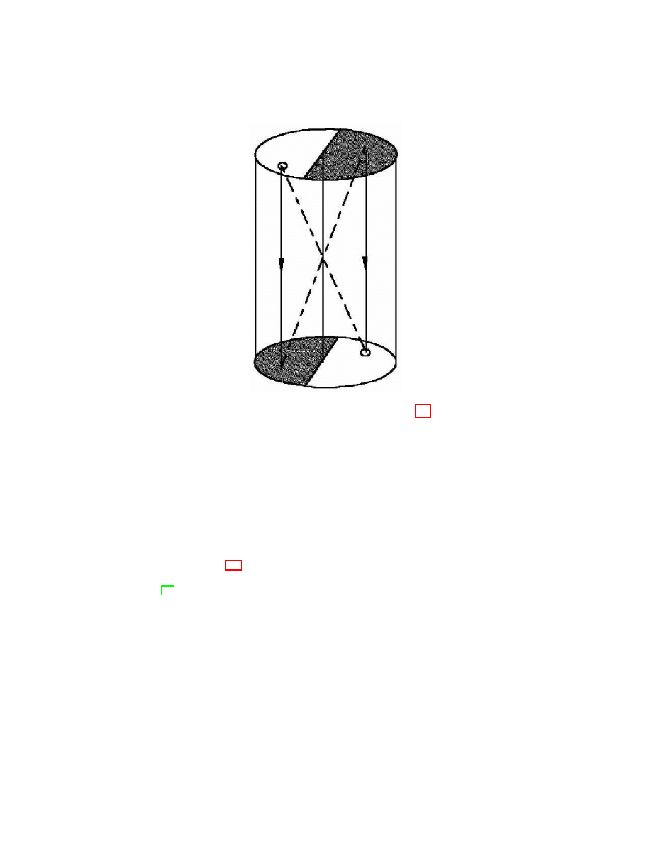
EJDE-2004/MON. 05
SINGULARITIES OF TRANSITION PROCESSES
31
Figure 5.
Phase space of the system (Example 3.3). All the
points of the axis are non-wandering; is the place of delay near
fixed points.
Lemma 3.5. A closed invariant set W is Lyapunov stable if and only if it has a
fundamental system of positively invariant closed neighborhoods: for any ε there
are such δ > 0 and closed positively invariant set V ⊂ X that
{x ∈ X : ρ
∗
(x, W ) < δ} ⊂ V ⊂ {x ∈ X : ρ
∗
(x, W ) < ε}.
(3.4)
To get the set V , one can take for example the closure of following (it is obviously
positively invariant) set: {f (t, x) : ρ
∗
(x, W ) ≤ δ = δ(ε/2), t ∈ [0, ∞)}, i.e. of the
complete image (for all t ≤ 0) of δ-neighbourhood of W , where δ(ε) is that spoken
about in Definition 3.4.
The following lemma can be deduced from the description of Lyapunov stable
sets ([80], Sec. 11, p.40-49).
Lemma 3.6. Let a closed invariant set W ⊂ X be not Lyapunov stable. Then
for any λ > 0 there is such y
0
∈ X that the y
0
-motion is whole, ρ
∗
(y
0
, W ) <
λ, d(α(y
0
), W ) < λ (i.e. the α-limit set of the y
0
-motion lies in λ-neighbourhood
of W ), and y
0
6∈ W .
Definition 3.7. An f -invariant set W ⊂ X for the semiflow f is called isolated, if
there is such λ > 0 that for any y ∈ ω
f
from the condition ρ
∗
(y, W ) < λ it follows
that y ∈ W , that is, any ω-limit point y ∈ ω
f
from the λ-neighbourhood of W
belongs to W .
Theorem 3.8. If for semiflow f there exists closed isolated and not Lyapunov
stable invariant set W ⊂ X then this semiflow possesses η
3
-slow relaxations.
32
A. N. GORBAN
EJDE-2004/MON. 05
Proof. Let W be a closed invariant isolated Lyapunov unstable set. Let λ > 0 be the
value from the definition of isolation. Then Lemma 3.6 guarantees the existence
of such y
0
∈ X that y
0
-motion is whole, ρ
∗
(y
0
, W ) < λ and y
0
6∈ W . It gives
(due to closure of W ) ρ
∗
(y
0
, W ) = d > 0. Let δ = min{d/2, (λ − d)/2}. Then δ-
neighbourhood of the point y
0
lies outside of the set W , but in its λ-neighbourhood,
and the last is free from the points of the set ω
f
\ W (isolation of W ). Thus, δ-
neighbourhood of the point y
0
is free from the points of the set ω
f
⊆ W
S(ω
f
\ W ),
consequently y
0
6∈ ω
f
. Since y
0
-motion is whole, Theorem 2.21 guarantees the
presence of η
3
-slow relaxations. Theorem 3.8 is proved.
Lemma 3.9. Let X be connected and ω
f
be disconnected, then ω
f
is not Lyapunov
stable.
Proof. Since ω
f
is disconnected, there are such nonempty closed W
1
, W
2
that
ω
f
= W
1
S W
2
and W
1
T W
2
= ∅. Since any x-trajectory is connected and ω
f
is invariant, then and W
1
and W
2
are invariant too. The sets ω(x) are connected
(see Proposition 1.6); therefore, for any x ∈ X ω(x) ⊂ W
1
or ω(x) ⊂ W
2
. Let us
prove that at least one of the sets W
i
(i = 1, 2) is not stable. Suppose the contrary:
W
1
and W
2
are stable. Define for each of them attraction domain:
At(W
i
) = {x ∈ X : ω(x) ⊂ W
i
}.
(3.5)
It is obvious that W
i
⊂ At(W
i
) owing to closure and invariance of W
i
. The sets
At(W
i
) are open due to the stability of W
i
. Really, there are non-intersecting
closed positively invariant neighborhoods V
i
of the sets W
i
, since the last do not
intersect and are closed and stable (see Lemma 3.5). Let x ∈ At(W
i
). Then there
is such t ≥ that f (t, x) ∈ int V
i
. But because of the continuity of f there is such
neighbourhood of x in X that for each its point x
0
f (t, x) ∈ int V
i
. Now positive
invariance and closure of V
i
ensure ω(x
0
) ⊂ W
i
, i.e. x
0
∈ At(W
i
). Consequently,
x lies in At(W
i
) together with its neighbourhood and the sets At(W
i
) are open
in X. Since At(W
i
)
S At(W
2
) = X, At(W
1
)
T At(W
2
) = ∅, the obtained result
contradicts to the connectivity of X. Therefore at least one of the sets W is not
Lyapunov stable. Prove that from this follows unstability of ω
f
. Note that if a
closed positively invariant set V is union of two non-intersecting closed sets, V =
V
1
S V
2
, V
1
T V
2
= ∅, then V
1
and V
2
are also positively invariant because of the
connectivity of positive semitrajectories. If ω
f
is stable, then it possess fundamental
system of closed positively invariant neighborhoods V
1
⊃ V
2
⊃ . . . V
n
⊃ . . . . Since
ω
f
= W
1
S W
2
, W
1
T W
2
= ∅ and W
i
are nonempty and closed, then from some
N V
n
= V
0
n
S V
00
n
= ∅ for n ≥ N , and the families of the sets V
0
n
⊃ V
0
n+1
⊃
. . . , V
00
n
⊃ V
00
n+1
. . . form fundamental systems of neighborhoods of W
1
and W
2
correspondingly. So long as V
0
n
, V
00
n
are closed positively invariant neighborhoods,
from this follows stability of both W
1
and W
2
, but it was already proved that it is
impossible. This contradiction shows that ω
f
is not Lyapunov stable and completes
the proof of the lemma.
Theorem 3.10. Let X be connected and ω
f
be disconnected. Then the semiflow f
possesses η
3
- and τ
1,2,3
-slow relaxations.
Proof. The first part (the existence of η
3
-slow relaxations) follows from Lemma
3.9 and Theorem 3.8 (in the last as a closed invariant set one should take ω
f
).
Let us prove the existence of τ
1
-slow relaxations. Let ω
f
be disconnected: ω
f
=
W
1
S W
2
, W
1
T W
2
= ∅, W
i
(i = 1, 2) are closed and, consequently, invariant due

EJDE-2004/MON. 05
SINGULARITIES OF TRANSITION PROCESSES
33
to the connectivity of trajectories. Consider the sets At(W
i
) (3.5). Note that at
least one of these sets At(W
i
) does not include any neighbourhood of W
i
. Really,
suppose the contrary: At(W
i
) (i = 1, 2) includes a ε-neighbourhood of W
i
. Let
x ∈ At(W
i
), τ = τ
1
(x, ε/3) be the time of the first entering of the x-motion into
ε/3-neighbourhood of the set ω(x) ⊂ W
i
. The point x possesses such neighbourhood
U ⊂ X that for any y ∈ U ρ(f (t, x), f (t, y)) < ε/3 as y ∈ U, 0 ≤ t ≤ τ . Therefore
d(f (τ, U ), W
i
) ≤ 2ε/3, U ⊂ At(W
i
). Thus, x lies in At(W
i
) together with its
neighbourhood: the sets At(W
i
) are open. This contradicts to the connectivity of
X, since X = At(W
1
)
S At(W
2
) and At(W
1
)
T At(W
2
) = ∅. To be certain, let
At(W
1
) contain none neighbourhood of W
1
. Then (owing to the compactness of X
and the closure of W
1
) there is a sequence x
i
∈ At(W
2
), x
i
→ y ∈ W
1
, ω(x
i
) ⊂
W
2
, ω(y) ⊂ W
1
. Note that r((x
i
), ω(y)) ≥ r(W
1
, W
2
) > 0, therefore there are
Ω(x)-bifurcations (y is the bifurcation point) and, consequently, (Theorem 2.9)
there are τ
1
-slow relaxations.
This yields the existence of τ
2,3
-slow relaxations
(τ
1
≤ τ
2
≤ τ
3
).
3.3. Slow Relaxations in Smooth Systems. In this subsection we consider the
application of the approach to the semiflows associated with smooth dynamical
systems developed above. Let M be a smooth (of class C
∞
) finite-dimensional
manifold, F : (−∞, ∞) × M → M be a smooth dynamical system over M , gener-
ated by vector field of class C
1
, X be a compact set positively invariant with respect
to the system F (in particular, X = M if M is compact). The restriction of F to
the set we call the semiflow over X, associated with F , and denote it by F |
X
.
We shall often use the following condition: the semiflow F |
X
has not non-
wandering points at the boundary of X (∂X); if X is positively invariant sub-
manifold of M with smooth boundary, int X 6= ∅, then this follows, for example,
from the requirement of transversality of the vector field corresponding to the sys-
tem F and the boundary of X. All the below results are valid, in particular, in the
case when X is the whole manifold M and M is compact (the boundary is empty).
Theorem 3.11. The complement of the set of smooth dynamical systems on com-
pact manifold M possessing the following attribute 1, is the set of first category (in
C
1
-topology in the space of smooth vector fields).
Attribute 1. Every semiflow F |
X
associated with a system F on any compact
positively invariant set X ⊂ M without non-wandering points on ∂X has not η
2
-
slow relaxations.
This theorem is a direct consequence of the Pugh closing lemma, the density
theorem [61, 57], and Theorem 3.2 of the present work.
Note that if X is positively invariant submanifold in M with smooth boundary,
int X 6= ∅, then by infinitesimal (in C
1
-topology) perturbation of F preserving
positive invariance of X one can obtain that semiflow over X, associated with the
perturbed system, would not have non-wandering points on ∂X. This can be easily
proved by standard in differential topology reasonings about transversality. In the
present case the transversality of vector field of “velocities” F to the boundary of
X is meant.
The structural stable systems over compact two-dimensional manifolds are stud-
ied much better than in general case [8, 58]. They possess a number of character-
istics which do not remain in higher dimensions. In particular, for them the set of
non-wandering points consists of a finite number of limit cycles and fixed points,

34
A. N. GORBAN
EJDE-2004/MON. 05
and the “loops” (trajectories whose α- and ω-limit sets intersect, but do not contain
points of the trajectory itself) are absent. Slow relaxations in these systems also
are different from the relaxations in the case of higher dimensions.
Theorem 3.12. Let M be C
∞
-smooth compact manifold, dim M = 2, F be a
structural stable smooth dynamical system over M , F |
X
be an associated with M
semiflow over connected compact positively invariant subset X ⊂ M . Then:
(1) For F |
X
the existence of τ
3
-slow relaxations is equivalent to the existence
of τ
1,2
- and η
3
-slow relaxations;
(2) F |
X
does not possess τ
3
-slow relaxations if and only if ω
F
T X consists of
one fixed point or of points of one limit cycle;
(3) η
1,2
-slow relaxations are impossible for F |
X
.
Proof. To prove the part 3, it is sufficient to refer to Theorem 3.2 and Proposition
2.3.
Let us prove the first and the second parts.
Note that ω
F |
X
= ω
F
T X.
Let ω
F
T X consist of one fixed point or of points of one limit cycle.
Then
ω(x) = X
T ω
F
for any x ∈ X. Also there are not such x ∈ X that x-motion
would be whole but not P
+
-stable and α(x)
T ω(x) 6= ∅ (owing to the structural
stability). Therefore (Theorem 2.20) τ
3
-slow relaxations are impossible. Suppose
now that ω
F
T X includes at least two limit cycles or a cycle and a fixed point or
two fixed points. Then ω
F |
X
is disconnected, and using Theorem 3.10 we obtain
that F |
X
possesses η
3
-slow relaxations. Consequently, exist τ
3
-slow relaxations.
From Corollary 2.22, i.e. the fact that every trajectory from ω
F
is a fixed point or
a limit cycle and also from the fact that rough two-dimensional systems have no
loops we conclude that τ
1
-slow relaxations do exist. Thus, if ω
F
T X is connected,
then F |
X
has not even τ
3
-slow relaxations, and if ω
F
T X is disconnected, then
there are η
3
and τ
1,2,3
-slow relaxations. Theorem 3.12 is proved.
In general case (for structural stable systems with dim M > 2) the statement 1
of Theorem 3.12 is not always true. Really, let us consider topologically transitive
U -flow F over the manifold M [5]; ω
F
= M , therefore η
3
(x, ε) = 0 for any X ∈
M, ε > 0. The set of limit cycles is dense in M . Let us choose two different
cycles P
1
and P
2
, whose stable (P
1
) and unstable (P
2
) manifolds intersect (such
cycles exist, see for example [68, 18]). For the point x of their intersection ω(x) =
P
1
, α(x) = P
2
, therefore x-motion is whole and not Poisson’s positively stable,
and (Lemma 2.17) τ
3
-slow relaxations exist. And what is more, there exist τ
1
-slow
relaxations too. These appears because the motion beginning at point near P
2
of x-trajectory delays near P
2
before to enter small neighbourhood of P
1
. It is
easy to prove the existence of Ω(x)-bifurcations too. Really, consider a sequence
t
1
→ ∞, from the corresponding sequence F (t
i
, x) choose convergent subsequence:
F (t
j
, x) → y ∈ P
2
, ω(y) = P
2
, ω(F (t
j
, x)) = P
1
, i.e. there are both τ
1
-slow
relaxations and Ω(x)-bifurcations. For A-flows a weaker version of the statement
1 of Theorem 3.12 is valid (A-flow is called a flow satisfying S.Smale A-axiom [68],
in regard to A-flows see also [18], p.106-143).
Theorem 3.13. Let F be an A-flow over compact manifold M . Then for any com-
pact connected positively invariant X ⊂ M which does not possess non-wandering
points of F |
X
on the boundary the existence of τ
3
-slow relaxations involves the
existence of τ
1,2
-slow relaxations for F |
X
.

EJDE-2004/MON. 05
SINGULARITIES OF TRANSITION PROCESSES
35
Proof. Note that ω
F |
X
= ω
f
T int X. If ω
F
T int X is disconnected, then, according
to Theorem 3.10, F |
X
possesses η
3
- and τ
1,2,3
-slow relaxations. Let ω
F
T int X be
connected. The case when it consists of one fixed point or of points of one limit
cycle is trivial: there are no any slow relaxations. Let ω
F
T int X consist of one
non-trivial (being neither point nor cycle) basic set (in regard to these basic sets
see [68, 18]): ω
F
T int X = Ω
0
. Since there are no non-wandering points over ∂X,
then every cycle which has point in X lies entirely in int X. And due to positive
invariance of X, unstable manifold of such cycle lies in X. Let P
1
be some limit
cycle from X. Its unstable manifold intersects with stable manifold of some other
cycle P
2
⊂ X [68]. This follows from the existence of hyperbolic structure on Ω
0
(see also [18], p.110). Therefore there is such x ∈ X that ω(x) = P
2
, α(x) = P
1
.
From this follows the existence of τ
1
- (and τ
2,3
-)-slow relaxations. The theorem is
proved.
Remark. We have used only very weak consequence of the hyperbolicity of the
set of non-wandering points: the existence in any non-trivial (being neither point
nor limit cycle) isolated connected invariant set of two closed trajectories, stable
manifold of one of which intersects with unstable manifold of another one. It seems
very likely that the systems for which the statement of Theorem 3.13 is true are
typical, i.e. the complement of their set in the space of flows is a set of first category
(in C
1
- topology).
4. Slow Relaxation of Perturbed Systems
4.1. Limit Sets of ε-motions. As models of perturbed motions let us take ε-
motions. These motions are mappings f
ε
: [0, ∞) → X, which during some fixed
time T depart from the real motions at most at ε.
Definition 4.1. Let x ∈ X, k ∈ K, ε > 0, T > 0. The mapping f
ε
: [0, ∞) → X
is called (k, ε, T )-motion of the point x for the system (1.1) if f
ε
(0) = x and for
any t ≥ 0, τ ∈ [0, T ]
ρ(f
ε
(t + τ ), f (τ, f
ε
(t), k)) < ε.
(4.1)
We call (k, ε, T )-motion of the point x (k, x, ε, T )-motion and use the denotation
f
ε
(t|x, k, T ).
It is obvious that if y = f
ε
(τ |x, k, T ) then the function f
∗
(t) =
f
ε
(t + τ |x, k, T ) is (k, y, ε)-motion.
The condition (4.1) is fundamental in study of motion with constantly function-
ing perturbations. Different restrictions on the value of perturbations of the right
parts of differential equations (uniform restriction, restriction at the average etc.,
see [9], p.184 and further) are used as a rule in order to obtain estimations analogous
to (4.1). On the base of these estimations the further study is performed.
Let us introduce two auxiliary functions:
ε(δ, t
0
) = sup{ρ(f (t, x, k), f (t, x
0
, k
0
)) : 0 ≤ t ≤ t
0
, ρ(x, x
0
) < δ, ρ
K
(k, k
0
) < δ};
(4.2)
δ(ε, t
0
) = sup{δ ≥ 0 : ε(δ, t
0
) ≤ ε}.
(4.3)
Due to the compactness of X and K the following statement is true.
Proposition 4.2. A) For any δ > 0 and t
0
> 0 the function ε(δ, t
0
) is defined;
ε(δ, t
0
) → 0 as δ → 0 uniformly over any compact segment t
0
∈ [t
1
, t
2
].
B) For any ε > 0 and t
0
> 0 the function δ(ε, t
0
) > 0 is defined (is finite).

36
A. N. GORBAN
EJDE-2004/MON. 05
Proof. A) Let δ > 0, t
0
> 0. Finiteness of ε(δ, t
0
) follows immediately from the
compactness of x. Let δ
i
> 0, δ
i
→ 0. Let us prove that ε(δ
i
, t
0
) → 0. Suppose
the contrary. In this case one can choose in {δ
i
} such subsequence that corre-
sponding ε(δ
i
, t
0
) are separated from zero by common constant: ε(δ
i
, t
0
) > α > 0.
Let us turn to this subsequence, preserving the same denotations. For every i
there are such t
i
, x
i
, x
0
i
, k
i
, k
0
i
that 0 ≤ t
i
≤ t
0
, ρ(x
i
, x
0
i
) < δ
i
, ρ
K
(k
i
, k
0
i
) < δ
i
and ρ(f (t
i
, x
i
, k
i
), f (t
i
, x
0
i
, k
0
i
)) > α > 0. The product [0, t
0
] × X × X × K × K is
compact. Therefore from the sequence (t
i
, x
i
, x
0
i
, k
i
, k
0
i
) one can choose a conver-
gent subsequence. Let us turn to it preserving the denotations: (t
i
, x
i
, x
0
i
, k
i
, k
0
i
) →
(˜
t, x
0
, x
0
0
, k
0
, k
0
0
). It is obvious that ρ(x
0
, x
0
0
) = ρ
K
(k
0
, k
0
0
) = ρ
K
(k
0
, k
0
0
) = 0, there-
fore x
0
= x
0
0
, k
0
= k
0
0
. Consequently, f (˜
t, x
0
, k
0
) = f (t, x
0
0
, k
0
0
). On the other hand,
ρ(f (t
i
, x
i
, k
i
), f (t
i
, x
0
i
, k
0
i
)) > α > 0, therefore ρ(f (˜
t, x
0
, k
0
), f (˜
t, x
0
0
, k
0
0
)) ≥ α > 0
and f (˜
t, x
0
, k
0
) 6= f (˜
t, x
0
0
, k
0
0
). The obtained contradiction proves that ε(δ
i
, t
0
) → 0.
The uniformity of tending to 0 follows from the fact that for any t
1
, t
2
> 0, t
1
< t
2
the inequality ε(δ, t
1
) ≤ ε(δ, t
2
) is true, ε(δ, t) is a monotone function.
The statement of the point B) follows from the point A).
The following estimations of divergence of the trajectories hold. Let f
ε
(t|x, k, T )
be (k, x, ε, T )-motion. Then
ρ(f
ε
(t|x, k, T ), f (t, x, k)) ≤ χ(ε, t, T ),
(4.4)
where χ(ε, t, T ) =
P
[t/T ]
i=0
κ
i
, κ
0
= ε, κ
i
= ε(κ
i−1
, T ) + ε.
Here and further
trivial verifications that follow directly from the triangle inequality are omitted. Let
f
ε
1
(t|x
1
, k
1
, T ), f
ε
2
(t|x
2
, k
2
, T ) be corresponding (k
1
, x
1
, ε
1
, T )- and (k
2
, x
2
, ε
2
, T )-
motions. Then
ρ(f
ε
1
(t|x
1
, k
1
, T ), f
ε
2
(t|x
2
, k
2
, T ))
≤ ε(max{ρ(x
1
, x
2
, , ρ
K
(k
1
, k
2
)}, T ) + χ(ε
1
, t, T ) + χ(ε
2
, t, T ).
(4.5)
From Proposition 4.2 it follows that χ(ε, t, T ) → 0 as ε → 0 uniformly over any
compact segment t ∈ [t
1
, t
2
].
Let T
2
> T
1
> 0, ε > 0. Then any (k, x, ε, T
2
)-motion is (k, x, ε, T
1
)-motion, and
any (k, x, ε, T
1
)-motion is (k, x, χ(ε, T
2
, T
1
), T
2
)-motion. Since we are interested in
perturbed motions behavior at ε → 0, and χ(ε, T
2
, T
1
) → 0 as ε → 0, then the
choice of T is unimportant. Therefore, let us fix some T > 0 and omit references to
it in formulas ((k, x, ε)-motion instead of (k, x, ε, T )-motion and f
ε
(t|x, k) instead
of f
ε
(t|x, k, T )).
The following propositions allows us “to glue together” ε-motions.
Proposition 4.3. Let ε
1
, ε
2
> 0, f
ε
1
(t|x, k) be ε
1
-motion, τ > 0, and
f
ε
2
(t|f
ε
1
(τ |x, k), k) be ε
2
-motion. Then the mapping
f
∗
(t) =
(
f
ε
1
(t|x, k),
if 0 ≤ t ≤ τ ;
f
ε
2
(t − τ |f
ε
1
(τ |x, k), k),
if t ≥ τ,
is (k, x, 2ε
1
+ ε
2
)-motion.
Proposition 4.4. Let δ, ε
1
, ε
2
> 0, f
ε
1
(t|x, k) be ε
1
-motion, τ > 0, f
ε
2
(t|y, k
0
) be
ε
2
-motion, ρ
K
(k, k
0
) < δ, ρ(y, f
ε
1
(τ |x, k)) < δ. Then the mapping
f
∗
(t) =
(
f
ε
1
(t|x, k),
if 0 ≤ t < τ ;
f
ε
2
(t − τ |y, k),
if t ≥ τ,

EJDE-2004/MON. 05
SINGULARITIES OF TRANSITION PROCESSES
37
is (k, x, 2ε
1
+ ε
2
+ ε(δ, T ))-motion.
Proposition 4.5. Let δ
j
, ε
j
> 0, the numbers ε
j
, δ
j
are bounded above, x
j
∈ X,
k
j
∈ K, k
∗
∈ K, τ
0
> T , j = 0, 1, 2, . . . , i = 1, 2, . . . , f
ε
j
(t|x
j
, k
j
) be the ε
j
-
motions, ρ(f
ε
j
(τ
j
|x
j
, k
j
), x
j+1
) < δ
j
, ρ
K
(k
j
, k
∗
) < δ
j
/2. Then the mapping
f
∗
(t) =
(
f
ε
0
(t|x
0
, k
0
),
if 0 ≤ t < τ
0
;
f
ε
j
t −
P
i−1
j=0
τ
j
|x
j
, k
j
,
if
P
i−1
j=0
τ
j
≤ t <
P
i
j=0
τ
j
,
is (k
∗
, x
0
, β)-motion, where
β =
sup
0≤j<∞
{ε
j+1
+ ε(ε
j
+ δ
j
+ δ
j+1
+ ε(δ
j
, T ), T )}.
The proof of the propositions 4.3-4.5 follows directly from the definitions.
Proposition 4.6. Let x
i
∈ X, k
i
∈ K, k
i
→ k
∗
, ε
i
> 0, ε
i
→ 0, f
ε
i
(t|x
i
, k
i
) be
(k
i
, x
i
, ε
i
)-motions, t
i
> 0, t
i
> t
0
, f
ε
i
(t
i
|x
i
, k
i
) → x
∗
. Then (k
∗
, x
∗
)-motion is
defined over the segment [−t
0
, ∞) and f
ε
i
(t
0
+t|x
i
, k
i
) tends to f (t, x
∗
, k
∗
) uniformly
over any compact segment from [−t
0
, ∞).
Proof. Let us choose from the sequence {x
i
} a convergent subsequence (preserving
the denotations): x
i
→ x
0
. Note that f
ε
i
(t|x
i
, k
i
) → f (t, x
0
, k
∗
) uniformly over
any compact segment t ∈ [t
1
, t
2
] ⊂ [0, ∞); this follows from the estimations (4.5)
and Proposition 4.2. Particularly, f (t
0
, x
0
, k
∗
) = x
∗
. Using the injectivity of f , we
obtain that x
0
is a unique limit point of the sequence {x
i
}, therefore f
ε
i
(t
0
+t|y
i
, k
i
)
tends to f (t, x
∗
, k
∗
) = f (t
0
+ t, x
0
, k
∗
) uniformly over any compact segment t ∈
[t
1
, t
2
] ⊂ [−t
0
, ∞).
Proposition 4.7. Let x
i
∈ X, k
i
∈ K, k
i
→ K
∗
, ε
i
> 0, f
ε
i
(t|x
i
, k
i
) be (k
i
, x
i
, ε
i
)-
motions, t
i
> 0, t
i
→ ∞, f
ε
i
(t
i
|x
i
, k
i
) → x
∗
. Then (k
∗
, x
∗
)-motion is whole and
the sequence f
ε
i
(t + t
i
|x
i
, k
i
) defined for t > t
0
for any t
0
, from some i(t
0
) (for
i ≥ i(t
0
)) tends to f (t, x
∗
, k
∗
) uniformly over any compact segment.
Proof. Let t
0
∈ (−∞, ∞). From some i
0
t
i
> −t
0
. Let us consider the sequence of
(k
i
, f
ε
i
(t
i
+t
0
|x
i
, k
i
), ε
i
)-motions: f
ε
i
(t|f
ε
i
(t
i
+t
0
|x
i
, k
i
), k
i
) := f
ε
i
(t+t
i
+t
0
|x
i
, k
i
).
Applying to the sequence the precedent proposition, we obtain the required state-
ment (due to the arbitrariness of t
0
).
Definition 4.8. Let x ∈ X, k ∈ K, ε > 0, f
ε
(t|x, k) be (k, x, ε)-motion. Let us
call y ∈ X ω-limit point of this ε-motion, if there is such a sequence t
i
→ ∞ that
f
ε
(t
i
|x, k) → y. We denote the set of all ω-limit points of f
ε
(t|x, k) by ω(f
ε
(t|x, k)),
the set of all ω-limit points of all (k, x, ε)-motions under fixed k, x, ε by ω
ε
(x, k),
and
ω
0
(x, k) :=
\
ε>0
ω
ε
(x, k).
Proposition 4.9. For any ε > 0, γ > 0, x ∈ X, k ∈ K
ω
ε
(x, k) ⊂ ω
ε+γ
(x, k).
Proof. Let y ∈ ω
ε
(x, k). For any δ > 0 there are (k, x, ε)-motion f
ε
(t|x, k) and
subsequence t
i
→ ∞, for which ρ(f
ε
(t
i
|x, k), y) < δ. Let δ =
1
2
δ(γ, T ). As (k, x, ε +
γ)-motion let us choose
f
∗
(t) =
(
f
∗
(t|x, k),
if t 6= t
i
;
y,
if t = t
i
(i = 1, 2, . . . , t
i+1
− t
i
> T ).

38
A. N. GORBAN
EJDE-2004/MON. 05
y is the ω-limit point of f
∗
(t), therefore, y ∈ ω
ε+γ
(x, k).
Proposition 4.10. For any x ∈ X, k ∈ K the set ω
0
(x, k) is closed and k-
invariant.
Proof. From Proposition 4.9 it follows
ω
0
(x, k) =
\
ε>0
ω
ε
(x, k).
(4.6)
Therefore, ω
0
(x, k) is closed. Let us prove that it is k-invariant. Let y ∈ ω
0
(x, k).
Then there are such sequences ε
j
> 0, ε
j
→ 0, t
j
i
→ ∞ as i → ∞ (j = 1, 2, . . . )
and such family of (k, x, ε
j
)-motions f
ε
j
(t|x, k) that f
ε
j
(t
j
i
|x, k) → y as i → ∞ for
any j = 1, 2, . . . . From Proposition 4.7 it follows that (k, y)-motion is whole. Let
z = f (t
0
, y, k). Let us show that z ∈ ω
0
(x, k). Let γ > 0. Construct (k, x, γ)-motion
which has z as its ω-limit point.
Let t
0
> 0. Find such δ
0
> 0, ε
0
> 0 that χ(ε
0
, t
0
+ T, T ) + ε(δ
0
, t
0
+ T ) < γ/2
(this is possible according to Proposition 4.2). Let us take ε
j
< ε
0
and choose from
the sequence t
j
i
(i = 1, 2, . . . ) such monotone subsequence t
l
(l = 1, 2, . . . ) for which
t
l+1
− t
l
> t
0
+ T and ρ(f
ε
j
(t
l
|x, k), y) < δ
0
. Let
f
∗
(t) =
(
f
ε
j
(t|x, k),
if t 6∈ [t
l
, t
l
+ t
0
] for any l = 1, 2, . . . ;
f (t − t
l
, y, k),
if t ∈ [t
l
, t
l
+ t
0
] (l = 1, 2, . . . ).
z is the ω-limit point of this (k, x, γ)-motion.
If t
0
< 0, then at first it is necessary to estimate the divergence of the trajectories
for “backward motion”. Let δ > 0. Let us denote
˜
ε(δ, t
0
, k) = sup
ρ(x, x
0
) :
inf
0≤t≤−t
0
{ρ(f (t, x, k), f (t, x
0
, k)} ≤ δ
.
(4.7)
Lemma 4.11. For any δ > 0, t
0
< 0 and k ∈ K ˜
ε(δ, t
0
, k) is defined (finite).
˜
ε(δ, t
0
, k) → 0 as δ → 0 uniformly by k ∈ K and by t
0
from any compact segment
[t
1
, t
2
] ⊂ (−∞, 0].
The proof can be easily obtained from the injectivity of f (t, ·, k) and the com-
pactness of X, K (similarly to Proposition 4.2).
Let us return to the proof of Proposition 4.10. Let t
0
< 0. Find ε
0
> 0 and
δ
0
> 0 such that ˜
ε(χ(ε
0
, T − t
0
, T ), t
0
, K) + ˜
ε(δ
0
, t
0
− T, k) < γ/2. According to
Proposition 4.2 and Lemma 4.11 this is possible. Let us take ε
j
< ε
0
and choose
from the sequence t
j
i
(i = 1, 2, . . . ) such monotone subsequence t
l
(l = 1, 2, . . . )
that t
l
> −t
0
, ρ(f
ε
i
(t
l
|x, k), y) < δ
0
and t
l+1
− t
l
> T − t
0
. Suppose
f
∗
(t) =
(
f
ε
j
(t|x, k),
if t 6∈ [t
l
+ t
0
, t
l
] for any l = 1, 2, . . . ;
f (t − t
l
, y, k),
if t ∈ [t
l
+ t
0
, t
l
] (l = 1, 2, . . . ).
where f
∗
(t) is (k, x, γ)-motion, and z is the ω-limit point of this motion.
Thus, z ∈ ω
γ
(x, k) for any γ > 0. The proposition is proved.
Proposition 4.12. Let x ∈ ω
0
(x, k). Then for any ε > 0 there exists periodical
(k, x, ε)-motion (This is a version of C
0
-closing lemma).

EJDE-2004/MON. 05
SINGULARITIES OF TRANSITION PROCESSES
39
Proof. Let x ∈ ω
0
(x, k), ε > 0, δ =
1
2
δ(
ε
2
, T ). There is (x, k, δ)-motion, and x is
its ω-limit point: x ∈ (f
δ
(t), x, k). There is such t
0
> T that ρ(f
δ
(t
0
|x, k), x) < δ.
Suppose
f
∗
(t) =
(
x,
if t = nt
0
, n = 0, 1, 2, . . . ;
f
δ
(t − nt
0
|x, k),
if nt < t < (n + 1)t
0
.
Here f
∗
(t) is a periodical (k, x, ε)-motion with the period t
0
.
Thus, if x ∈ ω
0
(x, k), then (k, x)-motion possesses the property of chain recur-
rence [23]. The inverse statement is also true: if for any ε > 0 there is a periodical
(k, x, ε)-motion, then x ∈ ω
0
(x, k) (this is obvious).
Proposition 4.13. Let x
i
∈ X, k
i
∈ K, k
i
→ k
∗
, ε
i
> 0, ε
i
→ 0, f
ε
i
(t|x
i
, k
i
)
be (k
i
, x
i
, ε
i
)-motion, y
i
∈ ω(f
ε
i
(t|x
i
, k
i
)), y
i
→ y
∗
. Then y
∗
∈ ω
0
(y, k). If in
addition x
i
→ x
∗
then y
∗
∈ ω
0
(x, k).
Proof. Let ε > 0 and δ =
1
2
δ(
ε
2
, T ). It is possible to find such i that ε
i
< δ/2,
ρ
K
(k
i
, k
∗
) < δ, and ρ(f
ε
i
(t
j
|x
i
, k
i
), y
∗
) < δ for some monotone sequence t
j
→
∞, t
j+1
− t
j
> T . Suppose
f
∗
(t) =
(
y
∗
,
if t = t
j
− t
1
(j = 1, 2, . . . );
f
ε
i
(t + t
1
|x
i
, k
i
),
otherwise,
where f
∗
(t) is (k
∗
, y
∗
, ε)-motion, y
∗
∈ ω(f
∗
). Since ε > 0 was chosen arbitrarily,
y
∗
∈ ω
0
(y
∗
, k
∗
). Suppose now that x
i
→ x
∗
and let us show that y
∗
∈ ω
0
(x
∗
, k
∗
).
Let ε > 0, δ =
1
2
δ(
ε
2
, T ). Find such i for which ε
τ
< δ/2, ρ(x
i
, x
∗
) < δ, ρ
K
(k
i
, k
∗
) <
δ and there is such monotone subsequence t
j
→ ∞ that t
1
> T , t
j+1
− t
j
> T ;
ρ(f
ε
i
(t
j
|x
i
, k
i
), y
∗
) < δ. Suppose
f
∗
(t) =
x
∗
,
if t = 0;
y
∗
,
if t = t
j
(j = 1, 2, . . . );
f
ε
i
(t|x
i
, k
i
),
otherwise,
where f
∗
(t) is (k
∗
, x
∗
, ε)-motion and y
∗
∈ ω(f
∗
). Consequently, y ∈ ω
0
(x
∗
, k
∗
).
Corollary 4.14. If x ∈ X, k ∈ K, y
∗
∈ ω
0
(x, k) then y
∗
∈ ω
0
(y
∗
, k).
Corollary 4.15. Function ω
0
(x, k) is upper semicontinuous in X × K.
Corollary 4.16. For any k ∈ K
ω
0
(k) :=
[
x∈X
ω
0
(x, k) =
[
x∈X
\
ε>0
ω
ε
(x, k) =
\
ε>0
[
x∈X
ω
ε
(x, k).
(4.8)
Proof. The inclusion
S
x∈X
T
ε>0
ω
ε
(x, k) ⊂
T
ε>0
S
x∈X
ω
ε
(x, k) is obvious.
To
prove the equality, let us take arbitrary element y of the right part of this inclusion.
For any natural n there is such x
n
∈ X that y ∈ ω
1/n
(x
n
, k). Using Proposition
4.13, we obtain y ∈ ω
0
(y, k) ⊂
S
x∈X
T
ε>0
ω
ε
(x, k), and this proves the corollary.
Corollary 4.17. For any k ∈ K the set ω
0
(k) is closed and k-invariant, and the
function ω
0
(k) is upper semicontinuous in K.
Proof. The k-invariance of ω
0
(k) follows from the k-invariance of ω
0
(x, k) for any
x ∈ X, k ∈ K (Proposition 4.10), closure and semicontinuity follow from Proposi-
tion 4.13.

40
A. N. GORBAN
EJDE-2004/MON. 05
Note that the statements analogous to the Corollaries 4.15. and 4.17 are incorrect
for the true limit sets ω(x, k) and ω(k).
Proposition 4.18. Let k ∈ K, Q ⊂ ω
0
(k) and Q be connected. Then Q ⊂ ω
0
(y, k)
for any y ∈ Q.
Proof. Let y
1
, y
2
∈ Q, ε > 0. Construct a periodical ε-motion which passes through
the points y
1
, y
2
. Suppose δ =
1
2
δ(
ε
2
, T ). With Q being connected, there is such
finite set {x
1
, . . . , x
n
} ⊂ Q that x
1
= y
1
, x
n
= y
2
and ρ(x
i
, x
i+1
) <
1
2
δ (i =
1, . . . , n − 1) and for every i = 1, . . . , n there is a periodical (k, x
i
, δ/2)-motion
f
δ/2
(t|x
i
, k) (see Proposition 4.12 and Corollary 4.14). Let us choose for every
i = 1, . . . , n such T
i
> T that f
δ/2
(T
i
|x
i
, k) = x
i
. Construct a periodical (k, y
1
, ε)-
motion passing through the points x
1
, . . . , x
n
with the period T
0
= 2
P
n
t=1
T
i
−
T
1
− T
n
: let 0 ≤ t ≤ T
0
, suppose
f
∗
(t)
=
f
δ/2
(tx
1
, k),
if 0 ≤ t < T ;
f
δ/2
t −
P
j−1
i=1
T
i
|x
i
, k
,
if
P
j−1
i=1
T
i
≤ t <
P
j
i=1
T
i
(j = 2, . . . , n);
f
δ/2
t −
P
n−1
i=1
T
i
+
P
n
i=j+1
T
i
|x
j
, k
,
if
P
n−1
i=1
T
i
+
P
n
i=j+1
T
i
≤ t <
P
n−1
i=1
T
i
+
P
n
i=j
T
i
.
If mT
0
≤ t < (m + 1)T
0
, then f
∗
(t) = f
∗
(t − mT
0
). f
∗
(t) is periodical (k, y
1
, ε)-
motion passing through y
2
. Consequently (due to the arbitrary choice of ε > 0),
y
2
∈ ω
0
(y, k) and (due to the arbitrary choice of y
2
∈ Q) Q ⊂ ω
0
(y
1
, k). The
proposition is proved.
Definition 4.19. Let us say that (1.1) possesses ω
0
(x, k)-(ω
0
(k)-)-bifurcations, if
the function ω
0
(x, k) (ω
0
(k)) is not lower semicontinuous (i.e. d-continuous) in
X × K. The point in which the lower semicontinuity gets broken is called the point
of (corresponding) bifurcation.
Proposition 4.20. If the system (1.1) possesses ω
0
-bifurcations, then it possesses
ω
0
(x, k)-bifurcations.
Proof. Assume that there exist ω
0
(k)-bifurcations. Then there are k
∗
∈ K (the
point of bifurcation), x
∗
∈ ω
0
(k
∗
), ε > 0, and sequence k
i
→ k, such that
ρ
∗
(x
∗
, ω
0
(k
i
)) > ε for any i = 1, 2, . . . .
Note that ω
0
(x
∗
, k
i
) ⊂ ω
0
(k
i
), consequently, ρ
∗
(x
∗
, ω
0
(x
∗
, k
i
)) > ε for any i.
However x
∗
∈ ω
0
(x
∗
, k
∗
) (Corollary 4.14). Therefore, d(ω
0
(x
∗
, k
∗
), ω
0
(x
∗
, k
i
)) >
ε, (x
∗
, k
∗
) is the point of ω
0
(x, k)-bifurcation.
Proposition 4.21. The sets of all points of discontinuity of the functions ω
0
(x, k)
and ω
0
(k) are subsets of first category in X × K and K correspondingly. For each
k ∈ K the set of such x ∈ X that (x, k) is the point of ω
0
(x, k)-bifurcation is
(k, +)-invariant.
Proof. The statement that the sets of points of ω
0
(x, k)- and ω
0
(k)-bifurcations
are the sets of first category follows from the upper semicontinuity of the functions
ω
0
(x, k) and ω
0
(k) and from known theorems about semicontinuous functions ([49,
p.78-81]). Let us prove (k, +)-invariance. Note that for any t > 0, ω
0
(f (t, x, k), k) =
ω
0
(x, k). If (x
i
, k
i
) → (x, k), of ω
0
(x, k)-bifurcation for any t > 0.

EJDE-2004/MON. 05
SINGULARITIES OF TRANSITION PROCESSES
41
Let (x
0
, k
0
) be the point of ω
0
(x, k)-bifurcation, Γ be a set of such γ > 0
for which there exist x
∗
∈ ω
0
(x
0
, k
0
) and such sequence (x
i
, k
i
) → (x
0
, k
0
) that
ρ
∗
(x
∗
, ω
0
(x
i
, k
i
)) ≥ γ for all i = 1, 2, . . . . Let us call the number ˜
γ = sup Γ the
value of discontinuity of ω
0
(x, k) in the point (x
0
, k
0
).
Proposition 4.22. Let γ > 0. The set of those (x, k) ∈ X × K, in which the
function ω
0
(x, k) is not continuous and the value of discontinuity ˜
γ ≥ γ, is nowhere
dense in X × K.
The proof can be easily obtained from the upper semicontinuity of the functions
ω
0
(x, k) and from known results about semicontinuous functions [49, p.78-81].
Proposition 4.23. If there is such γ > 0 that for any ε > 0 there are (x, k) ∈
X × K for which d(ω
ε
(x, k), ω
0
(x, k)) > γ then the system (1.1) possesses ω
0
(x, k)-
bifurcations with the discontinuity ˜
γ ≥ γ.
Proof. Let the statement of the proposition be true for some γ > 0. Then there are
sequences ε
i
> 0, ε
i
→ 0 and (x
i
, k
i
) ∈ X × K, for which d(ω
ε
i
(x
i
, k
i
), ω
0
(x
i
, k
i
)) >
γ. For every i = 1, 2, . . . choose such point y
i
∈ ω
ε
i
(x
i
, k
i
) that ρ
∗
(y
i
, ω
0
(x
i
, k
i
)) >
γ. Using the compactness of X and K, choose subsequence (preserving the denota-
tions) in such a way that the new subsequences y
i
and (x
i
, k
i
) would be convergent:
y
i
→ y
0
, (x
i
, k
i
) → (x
0
, k
0
). According to Proposition 4.13 y
0
∈ ω
0
(x
0
, k
0
). For
any κ > 0 ρ
∗
(y
0
, ω
0
(x
i
, k
i
)) > γ − κ from some i = i(κ). Therefore (x
0
, k
0
) is the
point of ω
0
(x, k)-bifurcation with the discontinuity ˜
γ ≥ γ.
4.2. Slow Relaxations of ε-motions. Let ε > 0, f
ε
(t|x, k) be (k, x, ε)-motion,
γ > 0. Let us define the following relaxation times:
(a) τ
ε
1
(t|x, k), γ) = inf{t ≥ 0 : ρ
∗
(f
ε
(t|x, k), ω
ε
(x, k)) < γ};
(b) τ
ε
2
(f
ε
(t|x, k), γ) = meas{t ≥ 0 : ρ
∗
(f
ε
(t|x, k), ω
ε
(x, k)) ≥ γ};
(c) τ
ε
3
(f
ε
(t|x, k), γ) = inf{t ≥ 0 : ρ
∗
(f
ε
(t
0
|x, k), ω
ε
(x, k)) < γ for t
0
> t};
(d) η
ε
1
(f
ε
(t|x, k), γ) = inf{t ≥ 0 : ρ
∗
(t|x, k), ω
ε
(k)) < γ};
(e) η
ε
2
(f
ε
(t|x, k), γ) = meas{t ≥ 0 : ρ
∗
(f
ε
(t|x, k), ω
ε
(k)) ≥ γ};
(f) η
ε
3
(f
ε
(t|x, k), = inf{t ≥ 0 : ρ
∗
(f
ε
(t
0
|x, k), ω
ε
(k)) < γ for t
0
> t}.
Here meas{·} is the external measure, ω
ε
(k) =
S
x∈X
ω
ε
(x, k).
There are another three important relaxation times. They are bound up with
the relaxation of a ε-motion to its ω-limit set. We do not consider them in this
work.
Proposition 4.24. For any x ∈ X, k ∈ K, ε > 0, γ > 0 and (k, x, ε)-motion
f
ε
(t|x, k) the relaxation times (a)-(f ) are defined (finite) and the inequalities τ
ε
1
≤
τ
ε
2
≤ τ
ε
3
, η
ε
1
≤ η
ε
2
≤ η
ε
3
, τ
ε
i
≥ η
ε
i
(i = 1, 2, 3) are valid.
Proof. The validity of the inequalities is obvious due to the corresponding inclusions
relations between the sets or their complements from the right parts of (a)–(f). For
the same reason it is sufficient to prove definiteness (finiteness) of τ
ε
3
(f
ε
(t|x, k), γ).
Suppose the contrary: the set from the right part of (c) is empty for some x ∈
X, k ∈ K, γ > 0 and (k, x, ε)-motion f
ε
(t|x, k). Then there is such sequence
t
i
→ ∞ that ρ
∗
(f
ε
(t
i
|x, k), ω
ε
(x, k)) ≥ γ. Due to the compactness of X, from the
sequence f
ε
(t
i
|x, k) can be chosen a convergent one. Denote its limit as y. Then y
satisfies the definition of ω-limit point of (k, x, ε)-motion but does not lie in ω
ε
(x, k).
The obtained contradiction proves the existence (finiteness) of τ
3
(f
ε
(t|x, k), γ).

42
A. N. GORBAN
EJDE-2004/MON. 05
In connection with the introduced relaxation times (a)-(f) it is possible to study
many different kinds of slow relaxations: infiniteness of the relaxation time for given
ε, infiniteness for any ε small enough e.c. We confine ourselves to one variant only.
The most attention will be paid to the times τ
ε
1
and τ
ε
3
.
Definition 4.25. We say that the system (1.1) possesses τ
0
i
- (η
0
i
-)-slow relax-
ations, if there are such γ > 0, sequences of numbers ε
j
> 0, ε
j
→ 0, of points
(x
j
, k
j
) ∈ X×K, and of (k
j
, x
j
, ε
j
)-motions f
ε
j
(t|x
j
, k
j
) that τ
ε
j
i
(f
ε
j
(t|x
j
, k
j
), γ) →
∞ (η
ε
j
i
(f
ε
j
(t|x
j
, k
j
), γ) → ∞) as j → ∞.
Theorem 4.26. The system (1.1) possesses τ
0
3
-slow relaxations if and only if it
possesses ω
0
(x, k)-bifurcations.
Proof. Suppose that the system (1.1) possesses τ
3
0
-slow relaxations: There are such
γ > 0, sequences of numbers ε
j
> 0, ε
j
→ 0, of points (x
j
, k
j
) ∈ X × K and of
(k
j
, x
j
, ε
j
)-motions f
ε
j
(t|x
j
, k
j
) that
τ
ε
j
3
(f
ε
j
(t|x, k), γ) → ∞
(4.9)
as j → ∞. Using the compactness of X × K, choose from the sequence (x
j
, k
j
) a
convergent one (preserving the denotations): (x
j
, k
j
) → (x
∗
, k
∗
). According to the
definition of the relaxation time τ
ε
3
there is such sequence t
j
→ ∞ that
ρ
∗
(f
ε
j
(t
j
|x
j
, k
j
), ω
ε
j
(x
j
, k
j
)) ≥ γ.
(4.10)
Choose again from (x
j
, k
j
) a sequence (preserving the denotations) in such a
manner, that the sequence y
j
= f
ε
j
(t
j
|x
j
, k
j
) would be convergent: y
j
→ y
∗
∈ X.
According to Proposition 4.7 (k
∗
, y
∗
)-motion is whole and f
ε
j
(t
j
+ t|x
j
, k
j
) →
f (t, y
∗
, k
∗
) uniformly over any compact segment t ∈ [t
1
, t
2
]. Two cases are possible:
ω
0
(y
∗
, k
∗
)
T α(y
∗
, k
∗
) 6= ∅ or ω
0
(y
∗
, k
∗
)
T α(y
∗
, k
∗
) = ∅. We shall show that in the
first case there are ω
0
(x, k)-bifurcations with the discontinuity ˜
γ ≥ γ/2 ((y
∗
, k
∗
)
is the point of bifurcation), in the second case there are ω
0
(x, k)-bifurcations too
((p, k
∗
) is the point of bifurcation, where p is any element from α(y
∗
, k
∗
)), but the
value of discontinuity can be less than γ/2. We need four lemmas.
Lemma 4.27. Let x ∈ X, k ∈ K, ε > 0, f
ε
(t|x, k) be (k, x, k)-motion, t > 0, y =
f
ε
(t|x, k). Then ω
0
(y, k) ⊂ ω
2ε+σ
(x, k) for any σ > 0.
The proof is an obvious consequence of the definitions and Proposition 4.3.
Lemma 4.28. Let x ∈ X, k ∈ K, t
0
> 0, y = f (t
0
, x, k), , δ > 0, ε =
ε(χ(δ, t
0
, T ), T ) + δ. Then ω
δ
(x, k) ⊂ ω
ε
(y, k).
Proof. Let f
δ
(t|x, k) be (k, x, δ)-motion. Then
f
∗
(t) =
(
y,
if t = 0;
f
δ
(t + t
0
|x, k),
if t > 0,
(4.11)
is (k, y, ε)-motion, ω(f
∗
) ⊂ ω
ε
(y, k), and ω(f
∗
) = ω(f
δ
(t|x, k)).
Since ε(χ(δ, t
0
, T ), T ) → 0, for δ → 0 we obtain the following result.
Corollary 4.29. Let x ∈ X, k ∈ K, t
0
> 0, y = f (t
0
, x, k). Then ω
0
(x, k) =
ω
0
(y, k).

EJDE-2004/MON. 05
SINGULARITIES OF TRANSITION PROCESSES
43
Lemma 4.30. Let (k, y)-motion be whole and ω
0
(y, k)
T α(y, k) 6= ∅. Then y ∈
ω
0
(y, k).
Proof. Let ε > 0, p ∈ ω
0
(y, k)
T α(y, k). Construct a periodical (k, y, ε)-motion.
Suppose that δ =
1
2
δ(
ε
2
, T ). There is such t
1
> T that for some (k, y, δ)-motion
f
δ
(t|y, k)ρ(f
δ
(t
1
|y, k), p) < δ. There is also such t
2
< 0 that ρ(f (t
2
, y, k), p) < δ.
Then it is possible to construct a periodical (k, y, ε)-motion, due to the arbitrariness
of ε > 0 and y ∈ ω
0
(y, k).
Lemma 4.31. Let y ∈ X, k ∈ K, (k, y)-motion be whole. Then for any p ∈ α(y, k)
ω
0
(p, k) ⊃ α(y, k).
Proof. Let p ∈ α(y, k), ε > 0. Construct a periodical (k, p, ε)-motion. Suppose that
δ =
1
2
δ(ε, T ). There are two such t
1
, t
2
< 0 that t
1
− t
2
> T and ρ(f (t
1,2
, y, k), p) <
δ. Suppose
f
∗
(t) =
(
p,
if t = 0 or t = t
1
− t
2
;
f (t + t
2
|y, k),
if 0 < t < t
1
− t
2
,
where f
∗
(t + n(t
1
− t
2
)) = f
∗
(t). Periodical (k, p, ε)-motion is constructed. Since
ε > 0 is arbitrary, p ∈ ω
0
(p, k). Using Proposition 4.18 and the connectivity of
α(y, k), we obtain the required: α(y, k) ⊂ ω
0
(p, k).
Let us return to the proof of Theorem 4.26. Note that according to Proposition
4.23 if there are not ω
0
(x, k)-bifurcations with the discontinuity ˜
γ ≥ γ/2, then from
some ε
0
> 0 (for 0 < ε ≤ ε
0
)d(ω
ε
(x, k), ω
0
(x, k)) ≤ γ/2 for any x ∈ X, k ∈ K.
Suppose that the system has τ
0
3
-slow relaxations and does not possess ω
0
(x, k)-
bifurcations with the discontinuity ˜
γ ≥ γ/2. Then from (4.10) it follows that for
0 < ε ≤ ε
0
p
∗
(f
ε
j
(t
j
|x
j
, k
j
), ω
ε
(x
j
, k
j
)) ≥ γ/2.
(4.12)
According to Lemma 4.27 ω
0
(y
j
, k
j
) ⊂ ω
3ε
j
(x
i
, k
j
). Let 0 < κ < γ/2. From
some j
0
(for j > j
0
) 3ε
j
< ε
0
and ρ(f
ε
j
(t
j
|x
j
, k
j
), y
∗
) < γ/2 − κ. For j > j
0
from
(4.12) we obtain
ρ
∗
(y
∗
, ω
0
(y
j
, k
j
)) > κ.
(4.13)
If ω
0
(y
∗
, k
∗
)
T α(y
∗
, k
∗
) 6= ∅, then from (4.13) and Lemma 4.30 follows the exis-
tence of ω
0
(x, k)-bifurcations with the discontinuity ˜
γ ≥ γ/2. The obtained con-
tradiction (if ω
0
(y
∗
, k
∗
)
T α(y
∗
, k
∗
) 6= ∅ and there are not ω
0
(x, k)-bifurcations
with the discontinuity ˜
γ ≥ γ/2, then they are) proves in this case the existence
of ω
0
(x, k)-bifurcations with the discontinuity ˜
γ ≥ γ/2. If ω
0
(y
∗
, k
∗
)
T α(y
∗
, k
∗
) =
∅, then there also exist ω
0
(x, k)-bifurcations.
Really, let p ∈ α(y
∗
, k
∗
).
Con-
sider such a sequence t
i
→ −∞ that f (t
i
, y
∗
, k
∗
) → p. According to Corollary
4.29 ω
0
(f (t
i
, y
∗
, k
∗
), k
∗
) = ω
0
(y
∗
, k
∗
), consequently, according to Lemma 4.31,
d(ω
0
(p, k
∗
), ω
0
(f (t
i
, y
∗
, k
∗
)) ≥ d(α(y
∗
, k
∗
), ω
0
(y
∗
, k
∗
)) > 0 and there are ω
0
(x, k)-
bifurcations. The theorem is proved.
Note that inverse to Theorem 4.26 is not true: for unconnected X from the ex-
istence of ω
0
(x, k)-bifurcations does not follow the existence of τ
0
3
-slow relaxations.
Example 4.32. (ω
0
(x, k)-bifurcations without τ
0
3
-slow relaxations). Let X be a
subset of plane, consisting of points with coordinates (
1
n
, 0) and vertical segment
J = {(x, y)|x = 0, y ∈ [−1, 1]}. Let us consider on X a trivial dynamical system
f (t, x) ≡ x. In this case ω
0
f
((
1
n
, 0)) =
(
1
n
, 0)
, ω
0
f
((0, y)) = J . There are ω
0
(x, k)

44
A. N. GORBAN
EJDE-2004/MON. 05
bifurcations: (
1
n
, 0) → (0, 0) as n → ∞, ω
0
f
((
1
n
, 0)) =
(
1
n
, 0)
, ω
0
f
((0, 0)) = J . But
there are not τ
3
0
-slow relaxations: τ
ε
3
(f
ε
(t|x), γ) = 0 for any (x, ε)-motion f
ε
(t|x)
and γ > 0. This is associated with the fact that for any (x, ε)-motion and arbitrary
t
0
≥ 0 the function
f
∗
(t) =
(
f
ε
(t|x),
if 0 ≤ t ≤ t
0
;
f
ε
(t
0
|x),
if t ≥ t
0
is (x, ε)-motion too, consequently, each (x, ε)-trajectory consists of the points of
ω
ε
f
(x).
For connected X the existence of ω
0
(x, k)-bifurcations is equivalent to the exis-
tence of τ
0
3
-slow relaxations.
Theorem 4.33. Let X be connected. In this case the system (1.1) possesses τ
0
3
-slow relaxations if and only if it possesses ω
0
(x, k)-bifurcations.
One part of Theorem 4.33 (only if) follows from the Theorem 4.26. Let us put
off the proof of the other part of Theorem 4.33 till Subsection 4.4, and the remained
part of the present subsection devote to the study of the set of singularities of the
relaxation time τ
2
for perturbed motions.
Theorem 4.34. Let γ > 0, ε
i
> 0, ε
i
→ 0, (x
i
, k
i
) ∈ X × K, f
ε
i
(t|x
i
, k
i
) be
(k
i
, x
i
, ε
i
)-motions, τ
ε
i
2
(f
ε
i
(t|x
i
, k
i
), γ) → ∞. Then any limit point of the sequence
{(x
i
, k
i
)} is a point of ω
0
(x, k)-bifurcation with the discontinuity ˜
γ ≥ γ.
Proof. Let (x
0
, k
0
) be limit point of the sequence {(x
i
, k
i
)}. Turning to subsequence
and preserving the denotation, let us write down (x
i
, k
i
) → (x
0
, k
0
). Let X =
S
n
j=1
V
j
be a finite open covering of X. Note that
τ
ε
i
2
(f
ε
i
(t|x
i
, k
i
)γ)
≤
n
X
j=1
meas{t ≥ 0 : f
ε
j
(t|x
i
, k
i
) ∈ V
j
, ρ
∗
(f
ε
i
(t|x
i
, k
i
), ω
ε
i
(x
i
, k
i
)) ≥ γ}.
Using this remark, consider a sequence of reducing coverings. Let us find (similarly
to the proof of Theorem 3.2) such y
0
∈ X and subsequence in {(x
i
, k
i
)} (preserving
for it the previous denotation) that for any neighbourhood V of the point y
0
meas{t ≥ 0 : f
ε
i
(t|x
i
, k
i
) ∈ V, ρ(f
ε
i
(t|x
i
, k
i
), ω
ε
i
(x
i
, k
i
)) ≥ γ} → ∞.
Let us show that y
0
∈ ω
0
(x
0
, k
0
). Let ε > 0. Construct such a (k
0
, x
0
, ε)-motion
that y
0
is its ω-limit point. Suppose δ =
1
2
δ(
ε
3
, T ). From some i
0
(for i > i
0
) the
following inequalities are true: ρ(x
i
, x
0
) < δ, ρ
K
(k
i
, k
0
) < δ, ε
i
< δ, and
meas{t ≥ 0 : ρ(f
ε
i
(t|x
i
, k
i
), y
0
) < δ, ρ
∗
(f
ε
i
(t|x
i
, k
i
), ω
ε
i
(x
i
, k
i
)) ≥ γ} > T.
On account of the last of these inequalities for every i > i
0
there are such t
1
, t
2
> 0
that t
2
− t
1
> T and ρ(f
ε
i
(t
1,2
|x
i
, k
i
), y
0
) < δ. Let i > i
0
. Suppose
f
∗
(t) =
x
0
,
if t = 0;
f
ε
i
(t|x
i
, k
i
),
if 0 < t < t
2
, t 6= t
1
;
y
0
,
if t = t
1
.
If t ≥ t
1
, then f
∗
(t + n(t
2
− t
1
)) = f
∗
(t), n = 0, 1, . . . . By virtue of the construction
f
∗
is (k
0
, x
0
, ε)-motion, y
0
∈ ω(f
∗
). Consequently (due to the arbitrary choice of
ε > 0), y
0
∈ ω
0
(x
0
, k
0
). Our choice of the point y
0
guarantees that y
0
6∈ ω
ε
i
(x
i
, k
i
)

EJDE-2004/MON. 05
SINGULARITIES OF TRANSITION PROCESSES
45
from some i.
Furthermore, for any κ > 0 exists such i = i(κ) that for i >
i(κ) ρ
∗
(y
0
, ω
ε
i
(x
i
, k
i
) > γ − κ. Consequently, (x
0
, k
0
) is the point of ω
0
(x, k)-
bifurcation with the discontinuity ˜
γ ≥ γ.
Corollary 4.35. Let γ > 0. The set of all points (x, k) ∈ X × K, for which there
are such sequences of numbers ε
i
> 0, ε → 0, of points (x
i
, k
i
) → (x, k), and of
(k
i
, x
i
, ε
i
)-motions f
ε
i
(t|x
i
, k
i
) that τ
ε
i
2
(f
ε
i
(t|x
i
, k
i
), γ) → ∞, is nowhere dense in
X × K. The union of all γ > 0 these sets (for all γ > 0) is a set of first category
in X × K.
4.3. Smale Order and Smale Diagram for General Dynamical Systems.
Everywhere in this subsection one semiflow of homeomorphisms f on X is studied.
We study here the equivalence and preorder relations generated by semiflow.
Definition 4.36. Let x
1
, x
2
∈ X. Say that points x
1
and x
2
are f -equivalent
(denotation x
1
∼ x
2
), if for any ε > 0 there are such (x
1
, ε)- and (x
2
, ε)-motions
f
ε
(t|x
1
) and f
ε
(t|x
2
) that for some t
1
, t
2
> 0
f
ε
(t
1
|x
1
) = x
2
, f
ε
(t
2
|x
2
) = x
1
.
Proposition 4.37. The relation ∼ is a closed f -invariant equivalence relation: the
set of pairs (x
1
, x
2
), for which x
1
∼ x
2
is closed in X × K; if x
1
∼ x
2
and x
1
6= x
2
,
then x
1
- and x
2
-motions are whole and for any t ∈ (−∞, ∞) f (t, x
1
) ∼ f (t, x
2
). If
x
1
6= x
2
, then x
1
∼ x
2
if and only if ω
0
f
(x
1
) = ω
0
f
(x
2
), x
1
∈ ω
0
f
(x
1
), x
2
∈ ω
0
f
(x
2
).
Compare with [76, Ch.6, Sec. 1], where analogous propositions are proved for
equivalence relation defined by action functional.
Proof. Symmetry and reflexivity of the relation ∼ are obvious. Let us prove its
transitivity. Let x
1
∼ x
2
, x
2
∼ x
3
, ε > 0. Construct ε-motions which go from x
1
to x
3
, and from x
3
to x
1
, gluing together δ-motions, going from x
1
to x
2
, from x
2
to x
3
and from x
3
to x
2
, from x
2
to x
1
. Suppose that δ = ε/4. Then, according
to Proposition 4.3, as a result of the gluing we obtain ε-motions with required
properties. Therefore x
1
∼ x
3
.
Let us consider the closure of the relation ∼. Let ε > 0, x
i
, y
i
∈ X, x
i
→
x, y
i
→ y, x
i
∼ y
i
. Suppose δ =
1
2
δ(
ε
3
, T ). There is such i that ρ(x
i
, x) < δ
and ρ(y
i
, y) < δ. Since x
i
∼ y
i
, there are binding them δ-motions f
δ
(t|y
i
) and
f
δ
(t|x
i
) : f
δ
(t
1i
|x
i
) = y
i
, f
δ
(t
2i
|y
i
) = x
i
, for which t
1i
, t
2i
> 0. Suppose that
f
∗
1
(t) =
x,
if t = 0;
y,
if t = t
1i
;
f
δ
(t|x
i
),
if t 6= 0, t
1i
,
f
∗
(t) =
y,
if t = 0;
x,
if t = t
2i
;
f
δ
(t|y
i
),
if t 6= 0, t
2i
,
here f
∗
1
and f
∗
2
are correspondingly (x, ε)- and (y, ε)-motions, f
∗
1
(t
1i
) = y, f
∗
(t
2i
) =
x. Since was chosen arbitrarily, it is proved that x ∼ y. Let x
1,2
∈ X, x
1
∼ x
2
, x
1
6=
x
2
. Show that ω
0
f
(x
1
) = ω
0
f
(x
2
) and x
1,2
∈ ω
0
f
(x
1
). Let ε > 0, y ∈ ω
0
f
(x
2
).
Prove that y ∈ ω
ε
f
(x
1
). Really, let f
ε/3
(t|x
1
) be (x
1
, ε/3)-motion, f
ε/3
(t
0
|x
1
) =

46
A. N. GORBAN
EJDE-2004/MON. 05
x
2
, f
ε/3
(t|x
2
) be (x
2
, ε/3)-motion, y ∈ ω(f
ε/3
(f
ε/3
(t|x
2
)). Suppose
f
∗
(t) =
(
f
ε/3
(t|x
1
),
if 0 ≤ t ≤ t
0
;
f
ε/3
(t
0
|x
2
),
if t > t
0
,
here f
∗
is (x
1
, ε)-motion (in accordance with Proposition 4.3), y ∈ ω(f
∗
). Con-
sequently, y ∈ ω
ε
(x
1
) and, due to arbitrary choice of ε > 0, y ∈ ω
0
(x
1
). Sim-
ilarly ω
0
(x
1
) ⊂ ω
0
(x
2
); therefore, ω
0
(x
1
) = ω
0
(x
2
). It can be shown that x
1
∈
ω
0
f
(x
1
), x
2
∈ ω
0
f
(x
2
). According to Proposition 4.10, the sets ω
0
f
(x
1,2
) are invariant
and x
1,2
-motions are whole.
Now, let us show that if x
2
∈ ω
0
f
(x
1
) and x
1
∈ ω
0
f
(x
2
) then x
1
∼ x
2
. Let
x
2
∈ ω
0
f
(x
1
), ε > 0. Construct a ε-motion going from x
1
to x
2
. Suppose that
δ = δ =
1
2
δ(
ε
2
, T ). There is such a (x
1
, δ)-motion that x
2
is its ω-limit point:
f
δ
(t
1
|x
1
) → x
2
, t
1
→ ∞. There is such t
0
> 0 that ρ(f
δ
(t
0
|x
1
), x
2
) < δ. Suppose
that
f
∗
(t) =
f
δ
(t|x
1
),
if t 6= t
0
;
x
2
,
if t = t
0
,
where f
∗
(t) is (x
1
, ε)-motion and f
∗
(t
0
) = x
2
. Similarly, if x
1
∈ ω
0
f
(x
2
), then for
any ε > 0 exists (x
2
, ε)-motion which goes from x
2
to x
1
. Thus, if x
1
6= x
2
, then
x
1
∼ x
2
if and only if x
1
∈ ω
0
(x
2
) and x
2
∈ ω
0
f
(x
1
). In this case ω
0
f
(x
1
) = ω
0
f
(x
2
).
The invariance of the relation ∼ follows now from the invariance of the sets ω
0
f
(x)
and the fact that ω
0
f
(x) = ω
0
f
(f (t, x)) if f (t, x) is defined.
The proposition is
proved.
Let us remind, that topological space is called totally disconnected if there exist
a base of topology, consisting of sets which are simultaneously open and closed.
Simple examples of such spaces are discrete space and Cantor discontinuum.
Proposition 4.38. Factor space ω
0
f
/ ∼ is compact and totally disconnected.
Proof. This proposition follows directly from Propositions 4.18, 4.37 and Corollary
4.17.
Definition 4.39 (Preorder, generated by semiflow). Let x
1
, x
2
∈ X. Let say
x
1
% x
2
if for any ε > 0 exists such a (x
1
, ε)-motion f
ε
(t|x
1
) that f
ε
(t
0
|x
1
) = x
2
for some t
0
≥ 0.
Proposition 4.40. The relation % is a closed preorder relation on X.
Proof. Transitivity of % easily follows from Proposition 4.3 about gluing of ε-
motions. The reflexivity is obvious. The closure can be proved similarly to the
proof of the closure of ∼ (Proposition 4.37, practically literal coincidence).
Proposition 4.41. Let x ∈ X. Then
ω
0
f
(x) = {y ∈ ω
0
f
: x % y}.
Proof. Let y ∈ ω
0
f
(x). Let us show that x % y. Let ε > 0. Construct a ε-motion
going from x to y. Suppose δ =
1
2
δ(
ε
3
, T ). There is such a (x, δ)-motion f
δ
(t|x)
that y is its ω-limit point: f
δ
(t
j
|x) → for some sequence t
j
→ ∞. There is such
t
0
> 0 that ρ(f
δ
(t
0
|x), y) < δ. Suppose that
f
∗
(t) =
(
f
δ
(t|x),
if t 6= t
0
;
y,
if t = t
0
,

EJDE-2004/MON. 05
SINGULARITIES OF TRANSITION PROCESSES
47
here f
∗
(t) is (x, ε)-motion and f
∗
(t
0
) = y. Consequently, x % y. Now suppose
that y ∈ ω
0
f
, x % y. Let us show that y ∈ ω
0
f
(x). Let ε > 0. Construct such a
(x, ε)-motion that y is its ω-limit point. To do this, use Proposition 4.12 and Corol-
lary 4.14 and construct a periodical (y, ε/3)-motion f
ε/3
: f
ε/3
(nt
0
|y) = y, n =
0, 1, . . . .. Glue it together with (x, ε/3)-motion going from x to y(f
ε/3
(t
1
|x) = y):
f
∗
(t) =
(
f
ε/3
(t|x),
if 0 ≤ t ≤ t
1
;
f
ε/3
(t − t
1
|y),
if t ≥ t
1
,
where f
∗
(t) is (x, ε)-motion, y ∈ ω(f
∗
), consequently (ε > 0 is arbitrary), y ∈ ω
0
f
(x).
The proposition is proved.
We say that the set Y ⊂ ω
0
f
is saturated downwards, if for any y ∈ Y ,
{x ∈ ω
0
f
|y % x} ⊂ Y.
It is obvious that every saturated downwards subset in ω
0
f
is saturated also for the
equivalence relation ∼.
Proposition 4.42. Let Y ⊂ ω
0
f
be open (in ω
0
f
) saturated downwards set. Then
the set At
0
(Y ) = {x ∈ X : ω
0
f
(x) ⊂ Y } is open in X.
Proof. Suppose the contrary. Let x ∈ At
0
(Y ), x
i
→ x and for every i = 1, 2, . . .
there is y
i
∈ ω
0
f
(x
i
) \ Y . On account of the compactness of ω
0
f
\ Y there is a
subsequence in {y
i
}, which converges to y
∗
∈ ω
0
f
\ Y . Let us turn to corresponding
subsequences in {x
i
}, {y
i
}, preserving the denotations: y
i
→ y
∗
. Let us show that
y ∈ ω
0
f
(x). Let ε > 0. Construct a ε-motion going from x to y. Suppose that
δ =
1
2
δ(
ε
3
, T ). From some i
0
ρ(x
i
, x) < δ and ρ(y
i
, y
∗
) < δ. Let i > i
0
. There is
(x
i
, δ)-motion going from x
i
to y
i
: f
δ
(t
0
|x
i
) = y
i
(according to Proposition 4.41).
Suppose that
f
∗
(t) =
f
∗
,
if t = 0;
y
∗
,
if t = t
0
;
f
δ
(t|x
i
),
if t 6= 0, t
0
,
where f
∗
is (x, )-motion going from x to y
∗
. Since ε > 0 is arbitrary, from this it
follows that x % y
∗
and, according to Proposition 4.41, y
∗
∈ ω
0
f
(x). The obtained
contradiction (y
∗
∈ ω
0
f
(x) \ Y , but ω
0
f
(x)subsetY ) proves the proposition.
Theorem 4.43. Let x ∈ X be a point of ω
0
f
(x)-bifurcation. Then there is such
open in ω
0
f
saturated downwards set W that x ∈ ∂At
0
(W ).
Proof. Let x ∈ X be a point of ω
0
f
-bifurcation: there are such sequence x
i
→ x
and such y
∗
∈ ω
0
f
(x) that ρ
∗
(y
∗
, ω
0
f
(x
i
)) > α > 0 for all i = 1, 2, . . . . Let us
consider the set ω =
S
∞
i=1
ω
0
f
(x
i
). The set ω is saturated downwards (according
to Proposition 4.41). We have to prove that it possesses open (in ω
0
f
) saturated
downwards neighbourhood which does not contain y
∗
. Beforehand let us prove the
following lemma.
Lemma 4.44. Let y
1
, y
2
∈ ω
0
f
, y
1
6∈ ω
0
f
(y
2
). Then there exists such an open
saturated downwards set Y that y
2
∈ Y , y
1
/
∈ Y , and Y ⊂ ω
ε
f
(y
2
) for some ε > 0.

48
A. N. GORBAN
EJDE-2004/MON. 05
Proof. ω
0
f
(y
2
) =
T
ε>0
ω
ε
(y
2
) (according to Proposition 4.9). There are such ε
0
>
0, τ > 0 that if 0 < ε ≤ ε
0
then ρ
∗
(y
1
, ω
ε
(y
2
)) > λ.
This follows from the
compactness of X and the so-called Shura-Bura lemma [2, p.171-172]: let a subset
V of compact space be intersection of some family of closed sets. Then for any
neighbourhood of V exists a finite collection of sets from that family, intersection
of which contains in given neighbourhood. Note now that if ρ
∗
(z, ω
0
f
(y
2
)) < δ =
1
2
δ(
ε
3
, T ) and z ∈ ω
0
f
, then z ∈ ω
ε
f
(y
2
). Really, in this case there are such p ∈
ω
0
f
(y
2
), (y
2
, δ)-motion f
δ
(t|y
2
), and monotone sequence t
i
→ ∞ that ρ(z, p) <
δ, t
j+1
− t
j
> T and ρ(f
δ
(t
i
|y
2
), p) < δ. Suppose
f
∗
(t) =
(
f
δ
(t|y
2
),
if t 6= t
j
;
z,
if t = t
j
,
here f
∗
(t) is (y
2
, ε)-motion and z ∈ ω(f
∗
) ⊂ ω
ε
(y
2
). Strengthen somewhat this
statement. Let z ∈ ω
0
f
and for some n > 0 exist such chain {z
1
, z
2
, . . . , z
n
} ∈ ω
0
f
that y
2
= z
1
, z = z
n
and for any i = 1, 2, . . . , n − 1 either z
i
% z
i+1
or ρ(z
i
, z
i+1
) <
δ =
1
2
δ(
ε
7
, T ). Then z ∈ ω
ε
(y
2
) and such a (y
2
, ε)-motion that z is its ω-limit
point is constructed as follows. If z
i
% z
i+1
, then find (z
i
, δ)-motion going from
z
i
to z
i+1
, and for every i = 1, . . . , n find a periodical (z
i
, δ)-motion. If z
1
% z
2
,
then suppose that f
∗
1
is (z
1
, δ)-motion going from z
1
to z
2
, f
∗
1
(t
1
) = z
2
; and if
ρ(z
1
, z
2
) < δ, z
1
% z
2
, then suppose that f
∗
1
is a periodical (z
2
, δ)-motion and
t
1
> 0 is such a number that t
1
> T and f
∗
1
(t
1
) = z
2
. Let f
∗
1
, . . . , f
∗
k
, t
1
, . . . , t
k
be
already determined. Determine f
∗
k+1
. Four cases are possible:
(1) f
∗
is periodical (z
i
, δ)-motion, i < n, z
i
% z
i+1
, then f
∗
k+1
is (z
i
, δ)-motion
going from z
i
to z
i+1
f
∗
k+1
(t
k+1
) = z
i+1
;
(2) f
∗
k
is periodical (z
i
, δ)-motion, i < n, ρ(z
i
, z
i+1
) < δ, then f
∗
k+1
is periodical
(z
i+1
, δ)-motion, f
∗
k+1
(t
k+1
) = z
i+1
, t
k+1
> T ;
(3) f
∗
k
is (z
i
, δ)-motion going from z
i
to z
i+1
, then f
∗
k+1
is periodical (z
i+1
, δ)-
motion, f
∗
k+1
(t
k+1
) = z
i+1
, t
k+1
> T ;
(4) f
∗
k
is periodical (z
n
, δ)-motion, then the constructing is finished.
After constructing the whole chain of δ-motions f
∗
k
and time moments t
k
, let us
denote the number of its elements by q and assume that
f
∗
(t) =
z
1
,
if t = 0;
f
∗
1
(t),
if 0 < t ≤ t
1
;
f
∗
k
t −
P
k−1
j=1
t
j
,
if
P
k−1
j=1
t
j
< t ≤
P
k
j=1
t
j
(k < q);
f
∗
q
t −
P
q−1
j=1
t
j
,
if t >
P
q−1
j=1
t
j
.
Here f
∗
(t) is (y
2
, ε)-motion, and z
n
= z is its ω-limit point. The set of those z ∈ ω
0
f
for which exist such chains z
1
, . . . , z
n
(n = 1, 2, . . . ) is an openly-closed (in ω
0
f
)
subset of ω
0
f
, saturated downwards. Supposing 0 < ε ≤ ε
0
, we obtain the needed
result. Even more strong statement was proved: Y can be chosen openly-closed (in
ω
0
f
), not only open.
Let us return to the proof of Theorem 4.43. Since ω =
S
∞
i=1
ω
0
f
(x
i
) and each
z ∈ ω
0
f
(x
i
) has an open (in ω
0
f
) saturated downwards neighbourhood W
z
which does
not contain y
∗
, then the union of these neighborhoods is an open (in ω
0
f
) saturated
downwards set which includes ω but does not contain y
∗
. Denote this set by W :
EJDE-2004/MON. 05
SINGULARITIES OF TRANSITION PROCESSES
49
W =
S
z∈ω
W
z
. Since x
i
∈ At
0
(W ), x 6∈ At
0
(W ) and x
i
→ x, then x ∈ ∂At
0
(W ).
The theorem is proved.
The following proposition will be used in Subsection 4.4 when studying slow
relaxations of one perturbed system.
Proposition 4.45. Let X be connected, ω
0
f
be disconnected. Then there is such
x ∈ X that x-motion is whole and x 6∈ ω
0
f
. There is also such partition of ω
0
f
into
openly-closed (in ω
0
f
) subsets:
ω
0
f
= W
1
∪ W
2
,
W ∩ W
2
= ∅,
α
f
(x) ⊂ W
1
but
ω
0
f
(x) ⊂ W
2
.
Proof. Repeating the proof of Lemma 3.9 (the repetition is practically literal, ω
0
f
should be substituted instead of ω
f
), we obtain that ω
0
f
is not Lyapunov stable.
Then, according to Lemma 3.6, there is such x ∈ X that x-motion is whole and
x 6∈ ω
0
f
. Note now that the set α
f
(x) lies in equivalence class by the relation ∼,
and the set ω
0
f
is saturated by the relation ∼ (Proposition 4.37, Lemma 4.31).
α
f
(x)
T ω
0
f
(x) = ∅, otherwise, according to Proposition 4.37 and Lemma 4.30,
x ∈ ω
0
f
. Since ω
0
f
/ ∼ is totally disconnected space (Proposition 4.38), there exists
partition of it into openly-closed subsets, one of which contains image of α
f
(x) and
the other contains image of ω
0
f
(x) (under natural projection ω
0
f
→ ω
0
f
/ ∼). Proto-
types of these openly-closed sets form the needed partition of ω
0
f
. The proposition
is proved.
4.4. Slow Relaxations in One Perturbed System. In this subsection, as in the
preceding one, we investigate one semiflow of homeomorphisms f over a compact
space X.
Theorem 4.46. η
0
1
- and η
0
2
-slow relaxations are impossible for one semiflow.
Proof. It is enough to show that η
0
2
-slow relaxations are impossible. Suppose the
contrary: there are such γ > 0 and such sequences of numbers ε
i
> 0 ε
i
→ 0, of
points x
i
∈ X and of (x
i
, ε
i
)-motions f
ε
i
(t|x
i
) that η
ε
i
2
(f
ε
i
(t|x
i
), γ) → ∞. Similarly
to the proofs of the theorems 4.34 and 3.2, find a subsequence in {f
ε
i
(t|x
i
)} and
such y
∗
∈ X that ρ
∗
(y
∗
, ω
0
f
) ≥ γ and, whatever be the neighbourhood V of the
point y
∗
in X, meas{t ≥ 0 : f
ε
i
(t|x
i
) ∈ V } → ∞ (i → ∞, f
ε
i
(t|x
i
) belongs to the
chosen subsequence). As in the proof of Theorem 4.34, we have y
∗
∈ ω
0
f
(y
∗
) ⊂ ω
0
f
.
But, according to the constructing, ρ
∗
(y
∗
, ω
0
f
) ≥ γ > 0. The obtained contradiction
proves the absence of η
0
2
-slow relaxations.
Theorem 4.47. Let X be connected. Then, if ω
0
f
is connected then the semiflow
f has not τ
0
1,2,3
- and η
0
3
-slow relaxations. If ω
0
f
is disconnected, then f possesses
τ
0
1,2,3
- and η
0
3
-slow relaxations.
Proof. Let X and ω
0
f
be connected. Then, according to the propositions 4.37 and
4.38, ω
0
f
(x) = ω
0
f
for any x ∈ X. Consequently, ω
0
(x)-bifurcations are absent.
Therefore (Theorem 4.26) τ
3
-slow relaxations are absent. Consequently, there are
not other τ
0
i
- and η
0
i
-slow relaxations due to the inequalities τ
ε
i
≤ τ
ε
3
and η
ε
i
≤
τ
ε
3
(i = 1, 2, 3) 1,2,3) (see Proposition 4.24).
The first part of the theorem is
proved.
Suppose now that X is connected and ω
0
f
is disconnected. Let us use Proposition
4.45. Find such x ∈ X that x-motion is whole, x 6∈ ω
0
f
, and such partition of ω
0
f
into

50
A. N. GORBAN
EJDE-2004/MON. 05
openly-closed subsets ω
0
f
= W
1
S W
2
, W
1
T W
2
= ∅ that α
f
(x) ⊂ W
1
, ω
0
f
(x) ⊂
W
2
. Suppose γ =
1
3
r(W
1
, W
2
). There is such t
0
that for t < t
0
ρ
∗
(f (t, x), W
2
) > 2γ.
Let p ∈ α
f
(x), t
j
< t
0
, t
j
→ −∞, f (t
j
, x) → p. For each j = 1, 2, . . . exists such
δ
j
> 0 that for ε < δ
j
d(ω
ε
f
(f (t
j
, x)), ω
0
f
(f (t
i
, x))) < γ (this follows from the Shura-
Bura lemma and Proposition 4.10). Since ω
0
f
(f (t
j
, x)) = ω
0
f
(x) (Corollary 4.29),
for ε < δ
j
d(ω
ε
f
(f (t
j
, x)), W
2
) < γ. Therefore ρ
∗
(f (t, x), ω
ε
f
(f (t
j
, x))) > γ if t ∈
[t
j
, t
0
], ε > δ
j
. Suppose x
i
= f (t
j
, x), ε
j
> 0, ε
j
< δ
j
, ε
j
→ 0, f
ε
j
(t|x
j
) = f (t, x
j
).
Then τ
ε
j
1
(f
ε
j
(t|x
j
), γ) ≥ t
0
− t
i
→ ∞. The existence of τ
1
- (and consequently of
τ
2,3
-)-slow relaxations is proved. To prove the existence of η
3
-slow relaxations we
need the following lemma.
Lemma 4.48. For any ε > 0 and κ > 0, ω
ε
f
⊂ ω
ε+κ
f
.
Proof. Let y ∈ ω
ε
f
: there are such sequences of points x
i
∈ X, y
i
∈ ω
ε
f
, of (x
i
, ε)-
motions f
ε
(t|x
i
), of numbers t
i
j
> 0, t
i
j
→ ∞ as j → ∞ that y
i
→ y, f
ε
(t
i
j
|x
i
) →
y
i
as j → ∞. Suppose that δ =
1
2
δ(
κ
3
, T ). There is such y
i
that ρ(y
i
, y) < δ.
For this y
i
there is such monotone sequence t
j
→ ∞ that t
j
− t
j−1
> T and
ρ(y
i
, f
ε
(t
j
|x
i
)) < δ. Suppose
f
∗
(t) =
f
ε
(t|x
i
),
if t 6= t
j
;
y,
if t = t
j
(j = 1, 2, . . . ),
where f
∗
(t) is (x
i
, κ + ε)-motion and y ∈ ω(f
∗
). Consequently, y ∈ ω
ε+κ
f
. The
lemma is proved.
Corollary 4.49. ω
0
f
=
T
ε>0
ω
ε
f
.
Let us return to the proof of Theorem 4.47 and show the existence of η
0
3
-slow
relaxations if X is connected and ω
0
f
is not. Suppose that γ =
1
5
r(W
1
, W
2
). Find
such ε
0
> 0 that for ε < ε
0
d(ω
ε
f
, ω
0
f
) > γ (it exists according to Corollary 4.49
and the Shura-Bura lemma).
There is t
1
for which d(f (t
1
, x), ω
0
f
) > 2γ.
Let
t
j
< t
1
, t
j
→ −∞, x
j
= f (x
j
, x). As (x
j
, ε)-motions let choose true motions
f (t, x
j
). Suppose that ε
j
→ 0, 0 < ε
j
< ε
0
. Then η
ε
j
(f (t, x
j
), γ) > t
1
− t
j
→ ∞
and, consequently, η
0
3
-slow relaxations exist. The theorem is proved.
In conclusion of this subsection let us give the proof of Theorem 4.33. We consider
again the family of parameter depending semiflows.
Proof of Lemma 4.49. Let X be connected and ω
0
(x, k)-bifurcations exist. Even
if for one k ∈ K ω
0
(k) is disconnected, then, according to Theorem 4.47, τ
0
3
-slow
relaxations exist. Let ω
0
(k) be connected for any k ∈ K. Then ω
0
(x, k) = ω
0
(k)
for any x ∈ X, k ∈ K. Therefore from the existence of ω
0
(x, k)-bifurcations follows
in this case the existence of ω
0
(k)-bifurcations. Thus, Theorem 4.33 follows from
the following lemma which is of interest by itself.
Lemma 4.50. If the system (1.1) possesses ω
0
(k)-bifurcations, then it possesses
τ
0
3
- and η
0
3
-slow relaxations.
Proof. Let k
∗
be a point of ω
0
(k)-bifurcation: and there are such α > 0, y
∗
∈ ω
0
(k
∗
)
that ρ
∗
(y
∗
, ω
0
(k
i
)) > α > 0 for any i = 1, 2, . . . . According to Corollary 4.49 and
the Shura-Bura lemma, for every i exists δ
i
> 0 for which ρ
∗
(y
∗
, ω
δ
i
(k
i
)) > 2α/3.
Suppose that 0 < ε
i
≤ δ
i
, ε
i
→ 0. As the ε-motions appearing in the definition of
EJDE-2004/MON. 05
SINGULARITIES OF TRANSITION PROCESSES
51
slow relaxations take the real (k
i
, y
i
)-motions, where y
i
= f (−t
i
, y
∗
, k
∗
), and t
i
are
determined as follows:
t
i
= sup{t > 0 : ρ(f (t
0
, x, k), f (t
0
x, k
0
)) < α/3}
under the conditions t
0
∈ [0, t], x ∈ X, ρ
K
(k, k
0
) < ρ
K
(k
∗
, k
i
)}.
Note that ρ
∗
(f (t
i
, y
i
, k
i
), ω
ε
i
(k
i
)) ≥ α/3, consequently, η
ε
i
3
(f (t, y
i
, k
i
), α/4) > t
i
and t
i
→ ∞ as i → ∞. The last follows from the compactness of X and K (see
the proof of Proposition 4.2). Thus, η
0
3
-slow relaxations exist and then τ
0
3
-slow
relaxations exist too. Lemma 4.50 and Theorem 4.33 are proved.
Summary
In Sections 1-4 the basic notions of the theory of transition processes and slow
relaxations are stated. Two directions of further development of the theory are
possible: introduction of new relaxation times and performing the same studies for
them or widening the circle of solved problems and supplementing the obtained
existence theorems with analytical results.
Among interesting but unsufficiently explored relaxation times let us mention
the approximation time
τ (x, k, ε) = inf{t ≥ 0 : d(ω(x, k), f ([0, t], x, k)) < ε}
and the averaging time
τ
v
(x, k, ε, ϕ) = inf
n
t ≥ 0 :
1
t
0
Z
t
0
0
ϕ(f (τ, x, k))dτ − hϕi
x,k
< ε for t
0
> t
o
,
where ε > 0, ϕ is a continuous function over the phase space X,
hϕi
x,k
= lim
t→∞
1
t
Z
t
0
ϕ(f (t, x, k))dτ
(if the limit exists).
The approximation time is the time necessary for the motion to visit the ε-
neighbourhood of each its ω-limit point. The averaging time depends on continuous
function ϕ and shows the time necessary for establishing the average value of ϕ with
accuracy ε along the trajectory.
As the most important problem of analytical research, one should consider the
problem of studying the asymptotical behaviour under T → ∞ of “domains of
delay”, that is, the sets of those pairs (x, k) (the initial condition, parameter) for
which τ
i
(x, k, ε) > T (or η
i
(x, k, ε) > T ). Such estimations for particular two-
dimensional system are given in the work [10].
“Structurally stable systems are not dense”. It would not be exaggeration to say
that the so titled work by Smale [67] opened a new era in the understanding of dy-
namics. Structurally stable (rough) systems are those whose phase portraits do not
change qualitatively under small perturbations (accurate definitions with detailed
motivation see in [12]). Smale constructed such structurally unstable system that
any other system close enough to it is also structurally unstable. This result broke
the hopes to classify if not all then “almost all” dynamical systems. Such hopes
were associated with the successes of classification of two-dimensional dynamical
systems [3, 4] among which structurally stable ones are dense.
There are quite a number of attempts to correct the catastrophic situation with
structural stability: to invent such natural notion of stability, for which almost all

52
A. N. GORBAN
EJDE-2004/MON. 05
systems would be stable. The weakened definition of structural stability is proposed
in the works [21, 62, 63]: the system is stable if almost all trajectories change little
under small perturbations. This stability is already typical, almost all systems are
stable in this sense.
The other way to get rid of the “Smale nightmare” (the existence of domains of
structurally unstable systems) is to consider the ε-motions, subsequently consider-
ing (or not) the limit ε → 0. The picture obtained (even in limit ε → 0) is more
stable than the phase portrait (the accurate formulation see above in Section 4).
It seems to be obvious that one should first study those (more rough) details of
dynamics, which do not disappear under small perturbations.
The approach based on consideration of limit sets of ε-motions, in the form
stated here was proposed in the paper [30]. It is necessary to note the conceptual
proximity of this approach to the method of quasi-averages in statistical physics
[17]. By analogy, the stated approach could be called the method of “quasi-limit”
sets.
Unfortunately, elaborated analytical or numerical methods of studying (con-
structing or, wider, localizing) limit sets of ε-motions for dynamical systems of
general type are currently absent. However, the author does not give up the hope
for the possibility of elaboration of such methods.
Is the subject of this work in the “mainstream” of Dynamics? I don’t know, but
let us imagine an experimental situation: we observe a dynamic of a system. It
might be a physical or a chemical system, or just a computational model, the precise
nature of the system is not important. How long should we monitor the system
in order to study the limit behaviour? When does the transition process turn into
the limit dynamics? This work tries to state these problems mathematically and
to answer them, at least partially.
References
[1] Afraimovich V.S., Bykov V.V., Shilnikov L.P., Rise and structure of Lorenz attractor, Dokl.
AN SSSR 234, 2 (1977), 336–339.
[2] Aleksandrov P.S., Passynkov V.A. Introduction into dimension theory. Moscow: Nauka, 1973.
574 p.
[3] Andronov A.A., Leontovich E.A., Gordon I.I., Mayer A.G. Bifurcations theory for dynamical
systems on the plane. Moscow: Nauka, 1967. 488 p.
[4] Andronov A.A., Vitt A.A., Khaikin S.E. Oscillation theory. Moscow: Nauka, 1981. 568 p.
[5] Anosov D.V., Geodesic flows on closed Riemannian manifolds of negative curvature, Proc.
V.A. Steklov Math. Inst. 90 (1967).
[6] Anosov D.V., About one class of invariant sets of smooth dynamical systems, Proceedings of
International conference on non-linear oscillation, V.2. Kiev, 1970, 39–45.
[7] Auslander J., Filter stability in dynamic systems, SIAM J. Math. Anal., 8, 3 (1977), 573–579.
[8] de Baggis G.F., Rough systems of two differential equations, Uspekhi Matematicheskikh Nauk
10, 4 (1955), 101–126.
[9] Barbashin E.A., Introduction into stability theory. Moscow, Nauka, 1967. 223 p.
[10] Bykov V.I., Gorban A.N., Pushkareva T.P., Singularities of relaxation times in oxidation
reaction of CO on Pt, Teor. i exp. khimija 18, 4 (1982), 431–439.
[11] Arnold V.I., Small denominators and stability problems in classical and celestial mechanics,
Uspekhi Matematicheskikh Nauk 18, 6 (1963), 91–192.
[12] Arnold V.I. Additional chapters of the theory of ordinary differential equations. Moscow:
Nauka, 1978. 304 p.
[13] Arnold V.I., Varchenko A.N., Gusein-Zade S.M. The singularity of differentiable mappings.
V.1, Moscow: Nauka, 1982; V.2, Moscow: Nauka, 1984.
[14] Bajaj P.N., Stability in semiflows, Math. Mod. Econom., Amsterdam e.a., 1974, 403–408.

EJDE-2004/MON. 05
SINGULARITIES OF TRANSITION PROCESSES
53
[15] Bautin N.N., Leontovich E.A. Methods and ways of qualitative exploration of dynamical
systems on the plane. Moscow: Nauka, 1976. 496 p.
[16] Birkhof J.D., Dynamical systems. Moscow– Leningrad: Gostekhizdat, 1941. 320 p.
[17] Bogolubov N.N., Selected works on statistical physics. Moscow: Moscow State University
Press, 1979, p.193–269.
[18] Bowen R., Methods of symbolical dynamics. Moscow: Mir, 1979. 245 p.
[19] Bourbaki N., General topology. General structures. Moscow: Nauka, 1968. 272 p.
[20] Das K.M., Lakshmi S.S., Negative and weak negative attractors in semidynamical systems,
Func. ekvacioj 21, 1 (1978), 53–62.
[21] Dobrynskii V.A., Sharkovskii A.N., Typicalness of dynamical systems, whose almost all tra-
jectories are stable under uniformly influencing perturbations, Dokl. AN SSSR 211, 2 (1973),
273–276.
[22] Duboshin G.N., On the problem of motion stability under uniformly influencing perturba-
tions, Proceedings P.K. Sternberg Inst. of Astronomy 14, 1 (1940), 153–164.
[23] Easton H., Chain transitivity and the domain of influence of an invariant set, Lect. Notes
Math., V.668 (1978), p.95–102.
[24] Eigen M., De Maeyer Leo., Theoretical basis of relaxation spectroscopy, In: Investigations of
rates and mechanisms of reactions. Ed by G.G.Hammes. Jon Willey & Sons, 1974.
[25] Elokhin V.I., Bykov V.I., Slinko M.G., Yablonskii G.S., Some problems of dynamics of oxi-
dation reaction of CO on Pt, Dokl. AN SSSR 238, 3 (1978), 615–618.
[26] Franke J.E., Selgrade J.F., Hyperbolicity and chain recurrence, J. Different. Equat. 26, 1
(1977), 27–36.
[27] Franke J.E., Selgrade J.F., Hyperbolicity and cycles, Trans. Amer. Math. Soc. 245 (1978),
251–262.
[28] Germaidze V.E., Krasovskii N.N., On the stability under uniformly influencing perturbations,
Prikl. matem. i mech. 21, 6 (1957), 769–775.
[29] Glazman I.M., Relaxation on the surface with saddle points, Dokl. AN SSSR 161, 4 (1965),
750–752.
[30] Gorban A.N., Slow relaxations of perturbed systems. I (general results). Krasnoyarsk:
Preprint Computing Center USSR Academy of Sciences, 1980.
[31] Gorban A.N., Slow relaxations and bifurcations of omega-limit sets of dynamical systems,
PhD Thesis in Physics & Math (Differential Equations & Math.Phys), Kuibyshev, Russia,
1980.
[32] Gorban A.N., Cheresiz V.M., Slow relaxations and bifurcations of limit sets of dynamical
systems. Krasnoyarsk: Preprint Computing Center USSR Academy of Sciences, 1980.
[33] Gorban A.N., Cheresiz V.M., Slow relaxations of dynamical systems and bifurcations of ω-
limit sets, Dokl. AN SSSR 261, 5 (1981), 1050–1054.
[34] Gorban A.N., Cheresiz V.M., Elokhin V.I., Yablonskii G.S., Slow relaxations and critical
phenomena in catalytic reactions, In: Mathematical methods in chemistry. V.2. Qualitative
methods. Moscow: ZNIITEneftehim, 1980, 53–60.
[35] Gorban A.N., Elokhin V.I., Cheresiz V.M., Yablonskii G.S., Possible kinetic reasons of slow
relaxations of catalytic reactions, In: Non-stationary processes in catalysis. Part 1. Novosi-
birsk, 1979, 83–88.
[36] Gottschalk W.H., Bibliography for topological dynamics, Wesleyan Univ., 1966, 76 p.
[37] Gottschalk W.H., Hedlund G.A., Topological dynamics, Providence, Amer. Math. Soc. Col-
loquium Publ. 36, 1 (1955), 1–51.
[38] Gromov M., Entropy, homology and semialgebraic geometry. S´
eminaire Bourbaki, Vol.
1985/86. AstSerisque 145-146, (1987), 225-240.
[39] Hasselblatt, B., Katok, A. (Eds.), Handbook of Dynamical Systems, Vol. 1A, Elsevier, 2002.
[40] Kaloshin V.Yu. Prevalence in spaces of smooth mappings and a prevalent Kupka-Smale the-
orem, Dokl. Akad. Nauk 355, 3 (1997), 306–307.
[41] Katok A.B., Local properties of hyperbolic sets. Supplement I to [57], 214–232.
[42] Katok A., Hasselblat, B. Introduction to the Modern Theory of Dynamical Systems, Ency-
clopedia of Math. and its Applications, Vol. 54, Cambridge University Press, 1995.
[43] Kifer Yu.I., Some results concerning small stochastic perturbations of dynamical systems,
Teoriya verojatnostej i ee primenenija 19, 2 (1974), 514–532.
[44] Kifer Yu.I., About small stochastic perturbations of some smooth dynamical systems, Izv.
AN SSSR. Matematika 38, 5 (1974), 1091–1115.

54
A. N. GORBAN
EJDE-2004/MON. 05
[45] Kornfeld I.P., Sinai Ya.G., Fomin S.V., Ergodic theory, Moscow: Nauka, 1980. 383 p.
[46] Krasovskii N.N., Some problems of the motion stability theory, Moscow: Fizmatgiz, 1959.
[47] Kupka I., Contribution `
a la th´
eorie des champs g´
en´
eriques. Contrib. Diff. Eqs. 2 (1963),
457–484. Ibid 3, (1964), 411–420.
[48] Kuratovskii K., Topology, V.1 Moscow: Mir, 1966. 594 p.
[49] Kuratovskii K., Topology. V.2 Moscow: Mir, 1969. 624 p.
[50] Lorenz E.N., Deterministic nonperiodic flow, J. Atmos. Sci. 20, 1 (1963), 130–141.
[51] Malkin I.G., On the stability under uniformly influencing perturbations, Prikl. matem. i
mech. 8, 3 (1944), 241–245.
[52] Malkin I.G., The motion stability theory, Moscow: Nauka, 1966, 20–21 and 301–305.
[53] Martynjuk A.A., Gutovsky R., Integral inequalities and motion stability, Kiev: Naukova
dumka, 1979, p.139–179.
[54] McCan C., Negative escape time in semidynamical systems, Func. ekvacioj 20, 1 (1977),
37–39.
[55] Moser J., Convergent series expansions for quasiperiodic motions, Math. Ann. 169 (1977),
136–176.
[56] Nemytskii V.V., Stepanov V.V., Qualitative theory of differential equations, Moscow–
Leningrad.: Gostekhizdat, 1949. 550 p.
[57] Nitetsky Z., Introduction into differential dynamics, Moscow: Mir, 1975. 305 p.
[58] Piexoto M., Structural stability on two–dimensional manifolds, Topology 1, 1 (1962), 101–120.
[59] Pontrjagin L.S., Andronov A.A., Vitt A.A., On statistical consideration of dynamical systems,
Sov. Phys. JETPh 3, 3 (1933), 165–180.
[60] Poston T., Stuart I., Catastrophe theory and its applications. Moscow: Mir, 1980.
[61] Pugh Ch., The closing lemma, Amer. J. Math. 89, 4 (1967), 956–1009.
[62] Sharkovskii A.N., Stability of trajectories and dynamical systems in whole, In: 9-th Summer
Mathematical School, Kiev: Naukova dumka, 1976, p.349–360.
[63] Sharkovskii A.N., Structural theory of differentiable dynamical systems and weakly non-
wandering points, Abh. Akad. Wiss. DDR. Abt. Math., Naturwiss., Techn.
No.4 (1977),
193–200.
[64] Semjonov N.N., Chain reactions, Leningrad: Goskhimizdat, 1934. 555 p.
[65] Sibirskii K.S., Introduction into topological dynamics, Kishinev: AS Mold. SSR Press, 1970.
144 p.
[66] Smale S., Stable manifolds for differential equations and diffeomorphisms, Ann. Sc. Norm.
Sup. Pisa 18, (1963), 97–116.
[67] Smale S., Structurally stable systems are not dense, Amer. J. Math. 88 (1966), 491–496.
[68] Smale S., Differentiable dynamical systems, Bull. AMS 73 (1967), 747–817.
[69] Spivak S.I., Shabat A.B., Shmelev A.S., On induction period of chemical reactions, In: Non-
stationary processes in catalysis. Part 1. Novosibirsk: Inst. of Catalysis, 1979, 118–121.
[70] Stepanjanz G.A., On general propositions of qualitative theory of discrete and irreversible
continuous systems, Problemy Kibernetiki 44, (1979), 5–14.
[71] Strauss A., Yorke A.J., Identifying perturbations which preserved asymptotic stability, Bull.
Amer. Math. Soc. 22, 2 (1969), 513–518.
[72] Trezepizur A., Ombach J., Limit sets on pseudo-dynamical systems, Bull. Acad. Pol. Sci.
Ser. Math. Sci., Astron. et Phys. 22, 2 (1974), 157–160.
[73] Van’t-Hoff J.H., Studies in dynamic chemistry. Leningrad.: ONTI, 1936. 178 p.
[74] Ventzel A.D., Freidlin M.I., Small stochastic perturbations of dynamical systems, Uspekhi
Matematicheskikh Nauk 25, 1 (1970), 3–55.
[75] Ventzel A.D., Freidlin M.I., Some problems concerning stability under small stochastic per-
turbations, Teoriya verojatnostej i ee primenenija 17, 2 (1972), 281–295.
[76] Ventzel A.D., Freidlin M.I., Fluctuations in dynamical systems influenced by small stochastic
perturbations, Moscow: Nauka, 1979. 424 p.
[77] Walters P., On the pseudoorbit tracing property and its relationship to stability, Lect. Notes
Math. V. 668 (1978), 231–244.
[78] Yablonskii G.S., Bykov V.I., Gorban A.N., Elokhin V.I., Kinetic models of catalytic reactions,
The series of monographs “Comprehensive Chemical Kinetics”, Vol. 32, Compton R.G. ed.,
Elsevier, Amsterdam, 1991. XIV+396 p.
[79] Yomdin Y., A quantitative version of the Kupka–Smale theorem, Ergodic Theory Dynamical
Systems 5, 3 (1985), 449-472.

EJDE-2004/MON. 05
SINGULARITIES OF TRANSITION PROCESSES
55
[80] Zubov V.I., Stability of motion. Moscow: Vysshaya shkola, 1973. 272 p.
Alexander N. Gorban
ETH-Zentrum, Department of Materials,, Institute of Polymers, Polymer Physics, Son-
neggstr. 3, CH-8092 Z¨
urich, Switzerland
Institute of Computational Modeling SB RAS,, Akademgorodok, Krasnoyarsk 660036,
Russia
E-mail address: agorban@mat.ethz.ch
Wyszukiwarka
Podobne podstrony:
Natiello M , Solari H The user#s approach to topological methods in 3 D dynamical systems (WS, 2007)
Mathematica package for anal and ctl of chaos in nonlin systems [jnl article] (1998) WW
Kwiek, Marek Social Perceptions versus Economic Returns of the Higher Education The Bologna Process
Mirlin Statistics of energy levels and eigenfunctions in disordered systems (PR326, p259, 2000)(124s
M O Donell Sources of certainity in formal systems
Initial Assessments of Safeguarding and Counterintelligence Postures for Classified National Securit
Can we accelerate the improvement of energy efficiency in aircraft systems 2010 Energy Conversion an
Review of methods for demonstrating redundancy in DP systems for the offshore industry
Advanced Mechanics in Robotic Systems (Springer 2011 Ed1)
Bankowość II, Przesłanki i proces przebudowy polskiego systemu bankowego
Cleaning In Place Systems
Algorytm Procesu Uruchomena Komputera, Systemy operacyjne
Language Processing in Discourse A Key to Felicitous Translation M Doherty (2002)
Proces Uruchamiania XP, Systemy operacyjne
Context in Dynamic Interpretation
uproszczone ogloszenie o zamowieniu objetym dynamicznym system zakupow, ZAMÓWIENIA PUBLICZNE 3
Heater and Coolers in Ventilation Systems
więcej podobnych podstron