Mathematica package for analysis and control of chaos
in nonlinear systems

Jose´ Manuel Gutie´rrez

a

!

and Andre´s Iglesias

b

!

Department of Applied Mathematics, University of Cantabria, Santander 39005, Spain

(Received 27 April 1997; accepted 27 July 1998)

In this article a symbolic Mathematica package for analysis and control of chaos in discrete and
continuous nonlinear systems is presented. We start by presenting the main properties of chaos and
describing some commands with which to obtain qualitative and quantitative measures of chaos,
such as the bifurcation diagram and the Lyapunov exponents, respectively. Then we analyze the
problem of chaos control and suppression, illustrating the different methodologies proposed in the
literature by means of two representative algorithms

~linear feedback control and suppression by

perturbing the system variables

!. A novel analytical treatment of these algorithms using the

symbolic capabilities of Mathematica is also presented. Well known one- and two-dimensional
maps

~the logistic and He´non maps! and flows ~the Duffing and Ro¨ssler systems! are used

throughout the article to illustrate the concepts and algorithms.

© 1998 American Institute of

Physics.

@S0894-1866~98!01806-9#

INTRODUCTION

In recent years, increasing research activity in the field of
nonlinear systems has shown that simple dynamical models
can produce complex, seemingly random-looking behavior,
including the appearance of deterministic chaos. One of the
main features of deterministic chaos is its sensitive depen-
dence to the initial conditions. This means that the separa-
tion between two nearby orbits of the system grows expo-
nentially in time and, therefore, a long-term prediction of
the system is possible only in probabilistic terms, although
the system dynamics is described by deterministic equa-
tions

~deterministic chaos!. The inability to predict the be-

havior of dynamical systems in the presence of chaos
makes this situation undesirable in many practical situa-
tions

~electronic circuits, chemical reactions, etc.!, where

one is more interested in obtaining regular behavior. How-
ever, the possibility of controlling chaos offers a way to
avoid this problem. As we shall see, the different control-
ling algorithms proposed in the literature take advantage of
the deterministic nature of chaotic systems that defines
some regularity in their inner structure.

In this article we introduce a Mathematica package

that includes several tools both for analyzing discrete and
continuous systems and for controlling the chaotic behavior
appearing in these systems

~this package is available

at the World Wide Web site http://ccaix3.unican.es/

;gutierjm/software.html!. First, we introduce the basic
properties of nonlinear systems using the commands of the
package that apply in this situation. For instance, these
commands allow us to obtain periodic points and their sta-
bility regions of nonlinear systems as well as some quali-
tative and quantitative measures of chaos, such as the bi-

furcation

diagram

and

the

Lyapunov

exponents,

respectively. Next, we analyze the problems of chaos con-
trol and suppression by presenting their main ideas and
illustrating the different approaches by means of two rep-
resentative algorithms: the linear-feedback-control method
and algorithm suppression by perturbing the system vari-
ables. We also present a novel analytical treatment of these
algorithms using the symbolic capabilities of Mathematica.

To illustrate the concepts and algorithms presented in

the article, we use well-known examples of discrete maps

~the logistic and He´non maps! and continuous flows ~the
Duffing oscillator and the Ro¨ssler system

!. We also give

the code of some of the commands to illustrate the pro-
gramming style and the symbolic and functional capabili-
ties of Mathematica. However, for a full understanding of
these programs some knowledge on Mathematica is re-
quired

~see Ref. 1!.

I. SYMBOLIC ANALYSIS OF NONLINEAR SYSTEMS

One of the most popular and simple examples of the non-
linear dynamical system is the logistic map, which is given
by the quadratic map x

n

11

5 f (r,x

n

)

5rx

n

(1

2x

n

), defined

on the unit interval

~0,1!, for values of the parameter r

P@0,4#, and on the interval @2~1/2!,~3/2!# for rP@22,0#.

Logistic[r

–

]

ª

Function[x, r x (1

2

x)];

This map was originally used by ecologists to model

population growth.

2

Given an initial population x

0

, the

next year’s population is given by x

1

5 f (r,x

0

), where the

parameter r is a growth rate. Repeating this iterative pro-
cess, x

2

5 f (r,x

1

), and so on, the sequence of populations

corresponding to successive years is obtained. This se-
quence is called the orbit of the point x

0

. The powerful

Mathematica functional-programming techniques help us to

a

!

E-mail: [e-mail]; http://ccaix3.unican.es/

;gutierjm

b

!

E-mail: [e-mail]; http://ccaix3.unican.es/

;iglesias

608

COMPUTERS IN PHYSICS, VOL. 12, NO. 6, NOV/DEC 1998

© 1998 AMERICAN INSTITUTE OF PHYSICS 0894-1866/98/12

~6!/608/12/$15.00

implement several algorithms for computing orbits in an
intuitive and efficient form. For example, the command

Or-

bit[map, x0, n]

uses the

NestList

functional command to

compute the n-point orbits of the map associated with the
initial condition x0. On the other hand, the command

Itera-

tiveProcess[map, x0,

$

min,max

%

]

illustrates the iterative pro-

cess (x

n

,x

n

11

)

→(x

n

11

,x

n

11

)

→(x

n

11

,x

n

12

) in the delay

reconstruction phase space (x

n

,x

n

11

).

Orbit[map

–

,x0

–

,n

–

]

ª

NestList[map, x0, n];

IterativeProcess[map

–

,x0

–

,

$

min

–

,max

–%

]

ª

Module[

$

fr,orb

%

,

orb

5

Orbit[map,x0,50];

fr

5

MapThread[Line[

$$

#1,#1

%

,

$

#1,#2

%

,

$

#2,#2

%%

]&,

$

Drop[orb,

2

1],Drop[orb,1]

%

];

Show[Plot[

$

map[x],x

%

,

$

x,min,max

%

], Graphics[

$

fr

%

]] ]

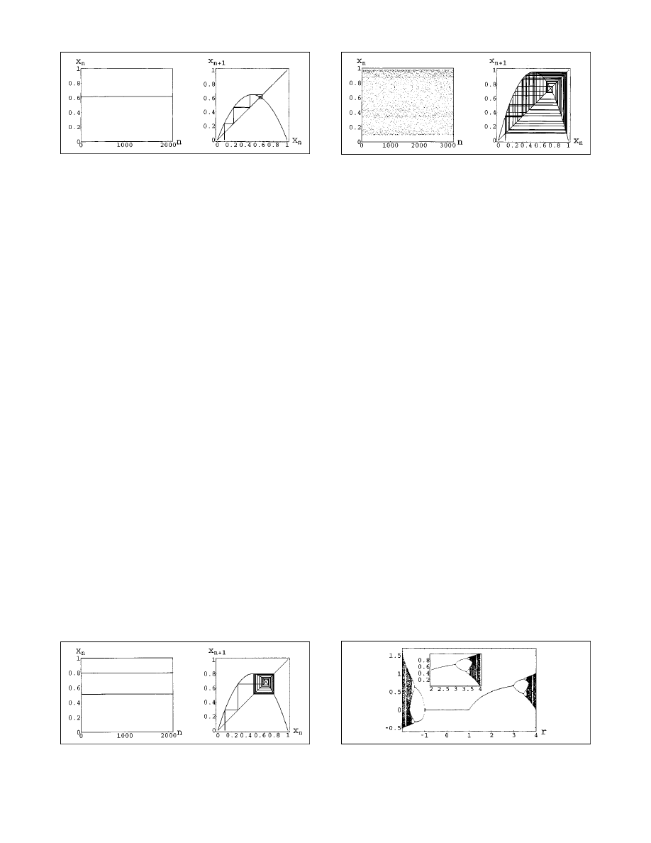
With the help of these commands we can analyze the

different system behaviors depending on the values of the
growth parameter. For certain values of this parameter, the
population settles to a fixed size over the years. This is
called a fixed point of the system

~see Fig. 1!.

Show[GraphicsArray[

$

ListPlot[Orbit[Logistic[2.6],0.1,100]],

IterativeProcess[Logistic[2.6],0.1,

$

0,1

%

]

%

]]

When the parameter value is increased, the system

jumps back and forth between two different points. This is
called a period-2 orbit

~see Fig. 2!.

Show[GraphicsArray[

$

ListPlot[Orbit[Logistic[3.2],0.1,100]],

IterativeProcess[Logistic[3.2],0.1,

$

0,1

%

]

%

]]

In addition, the system may also evolve under an in-

finite number of points in a random-looking form

~see Fig.

3

!. This behavior is known as deterministic chaos, since

seemingly stochastic

~chaotic! behavior is obtained from

the dynamics of a deterministic system.

Show[GraphicsArray[

$

ListPlot[Orbit[Logistic[3.9],0.1,100]],

IterativeProcess[Logistic[3.9],0.1,

$

0,1

%

]

%

]]

The different behaviors of the system for different val-

ues of the parameter can be qualitatively analyzed by using
a bifurcation diagram, which is created by plotting the
asymptotic orbits of the maps

~y axis! generated for differ-

ent values of the parameter

~x axis!. The command

Bifurca-

tion[map,

$

p,pi,pf,np

%

, n]

plots the bifurcation diagram of the

map consisting of n-point orbits

~after discarding an initial

transient

! for np equally spaced parameters in the region

p

5pi to p f .

Bifurcation[map

–

,

$

p

–

, pi

–

, pf

–

, np

–%

, n

–

]

ª

Module[

$

pp

%

,ListPlot[Flatten

[Table[(

$

pp,#

%

)& /@ Drop[Orbit[map /. p

→

pp][0.5,n

1

50],50],

$

pp,pi,pf,(pf

2

pi)/np

%

],1],

Axes

→

False,Frame

→

True,

PlotStyle

→$

PointSize[0.003]

%

]]

As an example, Fig. 4 shows the complete bifurcation

diagram of the logistic map, considering all the possible
values of the parameter in the range

~22,4!. Note that the

logistic map is usually defined for the parameter range

~0,4!, where the population of the system is normalized

~defined by the unit interval! and the parameter takes on
positive values. A detail of this region is shown in the inset
of Fig. 4.

Show[Graphics[

$

Rectangle[

$

0,0

%

,

$

1,1

%

,

Bifurcation[Logistic[r],

$

r,

2

2,4,250

%

,0.5,200,]],

Rectangle[

$

0.3,0.5

%

,

$

0.7,1

%

,

Bifurcation[Logistic[r],

$

r,0,4,100

%

, 0.5,200]]

%

]]

The dynamics observed in Figs. 1–3 can now be better

understood with the help of the bifurcation diagram. When
the value of the parameter r is increased from zero, the
system dynamics follow a sequence of period-1, -2, -4,...

Figure 1. Time series (left) and first return map (right) of the fixed point
logistic map with r

5

2.6 and x

0

5

0.1

Figure 2. Time series (left) and first return map (right) of the period-2
logistic map with r

5

3.2 and x

0

5

0.1

Figure 3. Time series (left) and first return map (right) of the chaotic
logistic map given by r

5

3.9 and x

0

5

0.1

Figure 4. Bifurcation diagram for the logistic map. The inset was created
by zooming into the region r

5

2 – 4.

COMPUTERS IN PHYSICS, VOL. 12, NO. 6, NOV/DEC 1998

609

orbits called period-doubling bifurcation route to chaos.
This sequence has universal properties for a large class of
maps

~for further details we refer the interested reader to

Ref. 12

!. When the parameter r is chosen beyond the criti-

cal accumulation parameter r

c

53.569..., the system be-

comes unpredictable and exhibits deterministic chaos.
Therefore, in this map deterministic chaos appears as a con-
sequence of the accumulation of an infinite number of un-
stable periodic orbits resulting of the period-doubling bifur-
cation process. This is another interesting property of chaos
known as orbit complexity

~see Ref. 4!. Orbit complexity

means that chaotic systems contain an infinite number of
unstable periodic orbits

~UPOs!, which coexist with the

strange attractor and play an important role in the system
dynamics.

5

This fact will be used later to control chaotic

behavior by stabilizing some of these unstable orbits.

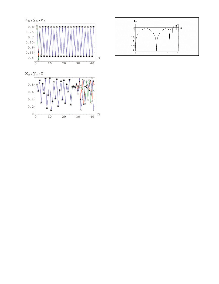
As we have already mentioned, the difference between

regular and chaotic behaviors can be established in terms of
their dependence on the initial conditions

~or perturbations

of the orbit

!. As shown in Fig. 5, periodic orbits are insen-

sitive to large perturbations of the initial conditions,
whereas chaotic orbits are very sensitive to tiny perturba-
tions.

MultipleListPlot[Orbit[Logistic[3.2],#,40]& /@

$

0.8, 0.8

1

0.02, 0.8

2

0.02

%

]

MultipleListPlot[Orbit[Logistic[3.9],#,40]& /@

$

0.8, 0.8

1

10 ˆ (

2

8), 0.8

2

10 ˆ (

2

8)

%

]

A quantitative measure of the sensitive dependence to

initial conditions is given by the Lyapunov exponents,
which measure the exponential separation of nearby orbits.
In simple terms, a positive Lyapunov exponent can be con-
sidered to be an indicator of chaos, whereas negative expo-
nents are associated with regular behavior

~periodic orbits!.

The

command

LyapunovExp[map,x0,n]

calculates

the

Lyapunov exponent of the one-dimensional

~1D! map

working with an n-point orbit starting at x0. In this case,
this exponent can be easily obtained by averaging the loga-
rithms of the map derivatives along the orbit.

3

LyapunovExp[map

–

,x0

–

,n

–

]

ª

Plus @@ (

Function[x,Evaluate[Log[Abs[D[map[x],x]]]]] /@
Drop[Orbit[map, x0, n

1

500],500])/n

As an example, Fig. 6 shows the Lyapunov spectrum

of the logistic map in the parameter range

~0,4!. If we com-

pare Fig. 6 with the bifurcation diagram shown in the inset
of Fig. 4, we can see how periodic regimes are associated
with negative Lyapunov exponents, whereas chaotic ones
have positive exponents.

Plot[Lyapunov[Logistic[r],0.5,500],

$

r,0,4

%

]

The rich structure of the bifurcation diagram and,

hence, of the system dynamics is a consequence of the
stable or unstable character of the periodic points for dif-
ferent values of the parameter. A fixed point x

f

is stable if

and only if it attracts nearby orbits, i.e.,

u@

]

x

f

~r,x!#

x

f

u

,1,

and unstable otherwise.
The command

PeriodicPoints[map, x, n]

obtains the period-

n fixed points of the map and the command

Stability[map, x,

r, fp, n]

gives the regions for the parameter r where the

period-n points f p are stable.

FixedPoints[map

–

,x

–

,n

–

]

ª

Simplify[Solve[Nest[map,x,n]

55

x,x]];

PeriodicPoints[map

–

,x

–

,n

–

]

ª

x/. Complement[FixedPoints[map,x,n],FixedPoints[map,x,
n-1]];

Stability[map

–

,x

–

,r

–

,fp

–

,n

–

]

ª

Module[

$

equ,s1,s2

%

,

equ

5

D[Nest[map,x,n],x] /. x

→

fp;

$

s1,s2

%5

Solve[equ

55

#, r]& /@

$2

1,1

%

;

If[s1!

5$%

&& s2!

5$%

, Sort /@

MapThread[List,

$

Flatten[r/. s1],Flatten[r/. s2]

%

],

$%

] ]

Figure 5. Three different orbits, x

n

, y

n

, and z

n

(in different colors),

corresponding to a periodic logistic map with initial conditions 0.8, and
0.8

6

0.02 (upper panel) and to a chaotic map with initial conditions 0.8

and 0.8

6

10

28

(lower panel).

Figure 6. Lyapunov exponent l

r

of the logistic map.

610

COMPUTERS IN PHYSICS, VOL. 12, NO. 6, NOV/DEC 1998

These commands help us to analyze the bifurcation

structure of the logistic map in an analytical form. For ex-
ample, the period-one points of the logistic map are

p1

5

PeriodicPoints[Logistic[r],x,1]

H

0,

r

21

r

J

which remain stable within the parameter regions

~21,1!

and

~1,3!, respectively, as obtained below.

Stability[Logistic[r],r,#,x,1]& /@ p1

$$$

21,1

%%

,

$$

1,3

%%%

Therefore, if

21,r,1, the fixed point (r21)/r is

unstable, whereas zero is stable. This implies that every
trajectory of the system will asymptotically fall to zero.
However, as r increases, the system presents a tangent bi-
furcation where the fixed point 0 loses its stability and the
fixed point (r

21)/r becomes stable @see interval ~1,3! in

Fig. 4

#. For larger values of the parameter, the fixed point

(r

21)/r becomes unstable and splits up into two different

period-2 points:

p2

5

PeriodicPoints[Logistic[r],x,2]

H

1

1r2

A

2322r1r

2

2r

,

1

1r1

A

2322r1r

2

2r

J

whose stability intervals are

Stability[Logistic[r],r,#,x,2]& /@ p2

$$$

21,12

A

6

%

,

$

3,1

1

A

6

%%

,

$$

21,12

A

6

%

,

$

3,1

1

A

6

%%%

In this case we have two stability regions for each of

the fixed points. Then, four period-4 points become stable,
and so on. Note that the calculation of periodic points with
larger periodicities involves polynomials of degrees larger
than five and, therefore, in general, they can only be ob-
tained numerically. In this case, the command

NFixed-

Points[map, x, n]

gives all the periodic points of the map up

to period n. For example, to illustrate the orbit complexity
phenomenon characteristic of chaotic systems, we can use
this command to obtain all the unstable periodic points up
to a given period

~e.g., n58! coexisting with the chaotic

attractor of the logistic map:

NFixedPoints[Logistic[3.9],x,8]

$

0.,0.00570386,0.00717971,0.0636502,0.0656863,0.0691803,0.0750764,

0.0917974,0.0919389,0.0974435,0.100562,0.104305,0.111837,0.114523,
0.121947,0.124823,0.132653,0.156816,0.180986,0.213536,0.237367,
0.289332,0.301209,0.358974,0.358974,0.385122,0.388375,0.413084,
0.43037,0.448718,0.465846,0.467459,0.476801,0.578097,0.619508,
0.697677,0.71665,0.74359,0.74359,0.74359,0.74359,0.75911,0.801914,
0.803777,0.827517,0.848259,0.897436,0.897436,0.9193,0.951213,0.964744

%

This phenomenon of creation and destruction of fixed

points as a transition to chaos is also present in higher-
dimensional discrete and continuous systems such as, for
example, the He´non map:

6

~x

n

11

, y

n

11

!5 f ~r,x

n

,y

n

!5~12rx

n

2

1y

n

,

1
3

x

n

!.

Henon[r

–

]

ª

Function

@

x,

$

1

2

r x

@@

1

##

ˆ 2

1

x

@@

2

##

, 1/3

x

@@

1

##

%

#

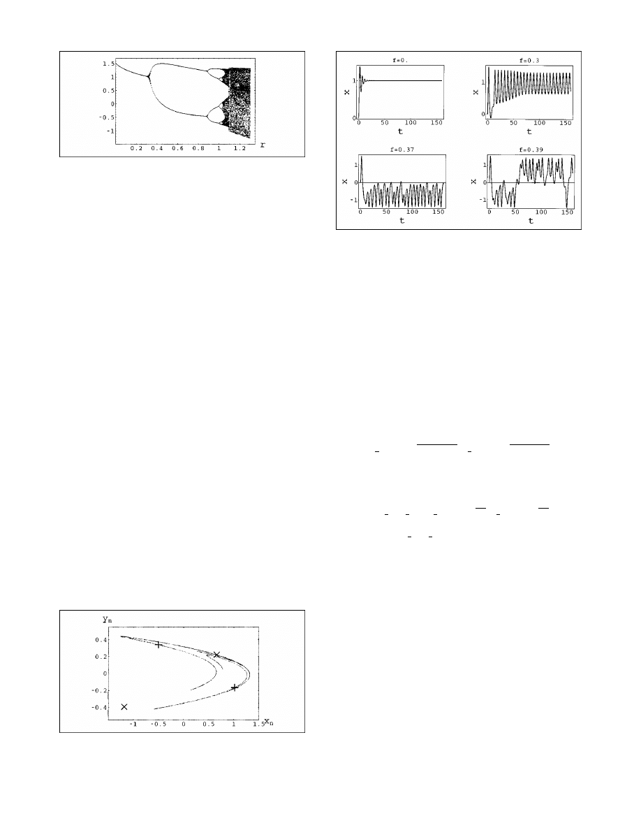
Depending on the values of the parameter r, this sys-

tem evolves among different behaviors associated with cha-
otic dynamics

~transient chaos, interior crisis, etc.!.

7

For

example, the system exhibits deterministic chaos for r
51.282. The bifurcation diagram associated with one of
the variables, say x, can be obtained as in the previous case
~see Fig. 7!:

Bifurcation[Henon[r],

$

r,0,1.3,250

%

,

$

0.5,0.5

%

,150]

In this case, we can also obtain the periodic points,

forming the period-doubling route to chaos, and study their
stability. For example, the period 1 and 2 points for the
He´non map can be obtained by

p1

5

PeriodicPoints[Henon[r],

$

x,y

%

,1]

HH

2

1

1

A

1

19r

3r

,

2

1

1

A

1

19r

9r

J

,

3

H

221

A

4

136r

6r

,

221

A

4

136r

18r

JJ

p2

5

PeriodicPoints[Henon[r],

$

x,y

%

,2]

HH

1

1

A

2319r

3r

,

2

211

A

2319r

9r

J

,

3

H

2

211

A

2319r

3r

,

1

1

A

2319r

9r

JJ

In this case, the stability of the fixed points depends on

the eigenvalues of the corresponding Jacobian matrix:

ev

5

Eigenvalues[D[Henon[r][

$

x,y

%

],#]& /@

$

x,y

%

]

$

1
6

~26rx2

A

12

136r

2

x

2

!,

1
6

~26rx1

A

12

136r

2

x

2

!

%

The next command shows that all these points are un-

stable, since they have associated a positive eigenvalue that
defines an unstable manifold. Fixed points with both posi-
tive and negative eigenvalues are called saddle nodes and
define stable and unstable manifolds. These points play a
key role in the context of chaos control.

8

COMPUTERS IN PHYSICS, VOL. 12, NO. 6, NOV/DEC 1998

611

(ev //.

$

x

→

#[[1]],r

→

1.282

%

)& /@ Union[p1,p2]

$$

20.2218,1.503

%

,

$

22.736,0.1218

%

,

$

20.1064,3.134

%

,

$

21.872,0.1781

%%

Figure 8 shows the strange attractor

~chaotic orbit! of

the He´non map for r

51.282 and (x

0

,y

0

)

5(0.5,0.5). Fig-

ure 8 also shows the periodic points obtained above.

MultipleListPlot[Orbit[Henon[1.282],

$

0.5,0.2

%

,2000],

p1/.r

→

1.282,p2/.r

→

1.282]

Deterministic chaos is also present in continuous non-

linear systems given by flows, i.e., systems of differential
equations. One of the most popular continuous nonlinear
systems is the Duffing oscillator, which includes damping
and periodic external forcing terms and is given by the
following second-order differential equation:

9

x

9

1ax

8

1x

3

2x5 f cos~

v

t

!,

or, equivalently, by the system of three first-order differen-
tial equations

H

x

8

5v

v

8

52av2x

3

1x1 f cos~z!,

z

8

5

v

,

where

v

5x

8

, z

5

v

t, a is the constant damping, and f and

v

are the strength and the frequency of the external forcing,

respectively. By fixing the values of constant damping and
external frequency, the oscillator exhibits a great variety of
behaviors as a function of the parameter f . In this example,
we take a

50.5 and

v

51.

Duffing[f

–

,w

–

]

ª$

v,

2

1/2

*

v

2

x ˆ 3

1

x

1

f

*

Cos[z], w

%

;

The fixed points of a flow can be obtained using the

command

FixedPointsFlow[flow,vars]

. In the case of the

nonlinear oscillator, in the absence of external forcing ( f
50), the system has two stable fixed points at
x

521 and x51 ~the positive one is shown in Fig. 9 la-

beled f

50!.

fp

5

FixedPointsFlow[Duffing[0,w],

$

x,v,z

%

]

$$

v

→0,x→21

%

,

$

v

→0,x→0

%

,

$

v

→0,x→1

%%

The stability of these fixed points is given by the ei-

genvalues of the corresponding Jacobian matrix:

ev

5

Eigenvalues[D[Duffing[0,w],#]& /@

$

x,v,z

%

]

$

0,

1
4

~212

A

17

248x

2

!,

1
4

~211

A

17

248x

2

!

%

The eigenvalues corresponding to each of the above

fixed points are

Re[ev /.fp]

$$

0,

2

1
4

,

2

1
4

%

,

$

0,

1
4

~212

A

17

!,

1
4

~211

A

17

!

%

,

3

$

0,

2

1
4

,

2

1
4

%

Therefore, x

521 and x51 are two stable fixed

points

~negative real parts of the eigenvalues! and x50 is

an unstable fixed point. When some forcing is applied to
the system, all the points become unstable and the system
oscillates around one of the fixed points with frequency
equal to the external frequency

v

~Fig. 9, f 50.3!. For val-

ues of the parameter f

.0.321 the system goes through a

period-doubling route to chaos. This period-doubling pro-
cess has an accumulation point at f

c

50.3586. Therefore,

larger values of the parameter lead to a chaotic system. For

f

c

, f ,0.386, the chaotic orbits of the system remain

trapped at one of the wells oscillating around a fixed point.
For example, Fig. 9 ( f

50.37) shows a chaotic orbit oscil-

lating around the unstable fixed point x

521. When in-

creasing the value of the parameter, the strange attractor
encompasses both wells

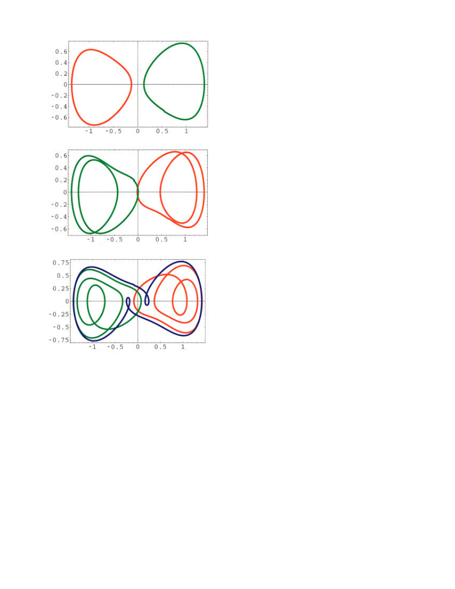
~Fig. 9, f 50.39!.

The command

OrbitFlow[flow, x, x0,

$

t0,t1,dt

%

]

imple-

ments a fourth-order Runge-Kutta method for systems of

Figure 7. Bifurcation diagram of the He´non map.

Figure 8. Chaotic attractor of the He´non map with two period-one and
two period-two points labeled as

3

and

1

, respectively.

Figure 9. Dynamics of the Duffing oscillator for different values of the
external forcing f .

612

COMPUTERS IN PHYSICS, VOL. 12, NO. 6, NOV/DEC 1998

first-order differential equations. This command is used in
the next example to calculate and plot several orbits, illus-
trating different behaviors of the Duffing oscillator.

Show[GraphicsArray[Show[

OrbitFlow[Duffing[#,1],

$

x,v,z

%

,

$

0.,1.,0.

%

,

$

0,160,0.05

%

,

Show

→

Plot]& /@

$

0.,0.3,0.37,0.39

%

] ]]

II. SELECTING UNSTABLE PERIODIC ORBITS

As we have indicated in Sec. I, the infinite number of un-
stable periodic orbits

~UPOs! embedded in the attractor

plays an important role in the behavior of chaotic systems.
However, in many practical situations one does not have
access to system equations and must deal directly with ex-
perimental data in the form of a time series.

10

Here in Sec.

II we give some commands for computing some of these
orbits from a time series of the system

~these commands

will be used later for controlling chaos

!.

A simple algorithm for obtaining a UPO searches for

closed ‘‘orbits’’ within the time series. Suppose we choose
an arbitrary point of the time series and wait until the orbit
comes back again to a small neighborhood of the selected
point

~the return neighborhood!. Then, we may conclude

that the orbit obtained shadows an unstable periodic orbit
of the system.

10

The command

UPO[timeseries,

e

, maxper]

obtains all the UPOs within the time series up to period
maxper considering

e

-radius balls as return neighborhoods.

For example, let us consider the following time series

obtained from the Duffing oscillator with f

50.39.

orb

5

Drop[#,

2

1]&/@

OrbitFlow[Duffing[0.39,1],

$

x,v,z

%

,

$

0,1,0

%

,

$

0,500,0.001

%

];

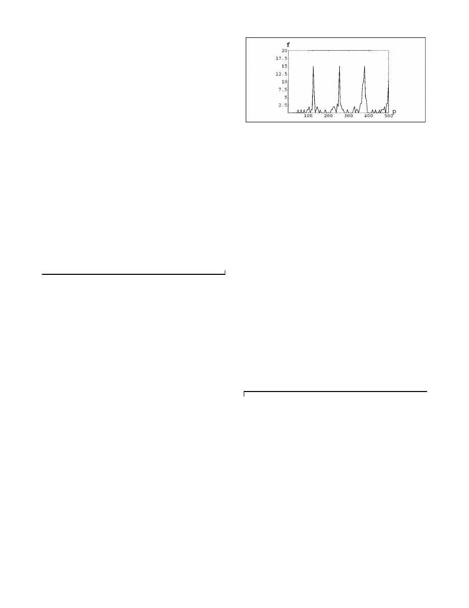
The commands

UPO, UPOFrequencies

~to obtain the

frequencies of UPOs of different periods

!, and

UPOHisto-

gram

~to obtain a histogram of the frequencies, as shown in

Fig. 10

! help us to understand the interwoven structure of

UPOs within the given series.

upos

5

UPO[orb,0.01,500];

UPOFrequencies[upos]
UPOHistogram[orb,500]

$$

50,1

%

,

$

62,1

%

,

$

78,1

%

,

$

91,1

%

,

$

100,1

%

,

$

101,1

%

,

$

105,1

%

,

$

113,1

%

,

$

119,1

%

,

$

123,1

%

,

$

124,10

%

,

$

125,4

%

,

$

126,5

%

,

$

129,1

%

,

$

139,1

%

,

$

141,1

%

,

$

145,1

%

,

$

149,1

%

,

$

158,1

%

,

$

183,1

%

,

$

213,1

%

,

$

218,1

%

,

$

221,1

%

,

$

222,1

%

,

$

228,1

%

,

$

229,1

%

,

$

235,1

%

,

$

244,1

%

,

$

245,2

%

,

$

246,1

%

,

$

248,1

%

,

$

252,2

%

,

$

253,2

%

,

$

254,4

%

,

$

255,7

%

,

$

256,1

%

,

$

259,2

%

,

$

263,1

%

,

$

264,1

%

,

$

266,1

%

,

$

275,1

%

,

$

292,1

%

,

$

323,1

%

,

$

328,1

%

,

$

329,1

%

,

$

337,1

%

,

$

344,1

%

,

$

351,1

%

,

$

359,2

%

,

$

360,1

%

,

$

361,1

%

,

$

363,1

%

,

$

364,1

%

,

$

366,1

%

,

$

367,1

%

,

$

368,1

%

,

$

369,3

%

,

$

370,3

%

,

$

371,3

%

,

$

372,4

%

,

$

374,2

%

,

$

375,1

%

,

$

376,5

%

,

$

377,5

%

,

$

379,2

%

,

$

380,3

%

,

$

382,3

%

,

$

383,1

%

,

$

385,1

%

,

$

386,1

%

,

$

387,1

%

,

$

388,1

%

,

$

390,1

%%

Finally, some of the obtained UPOs can be plotted by

using the

SelectUPO[timeseries,

$

minper,maxper

%

]

com-

mand, which selects from the time series all the unstable
orbits of periods in the range p

5minper to maxper. For

example, Fig. 11 shows several UPOs with periodicities
associated with the peaks of Fig. 10

~124, 252, 376!.

UPOPlot[orb,SelectUPO[upo,

$

#,#

%

]]& /@

$

124,252,376

%

III. CONTROLLING AND SUPPRESSING CHAOS

As we have shown in Sec. II, chaotic systems are charac-
terized by an exponential separation of nearby orbits in
time. This feature of chaos has been traditionally seen as a
troublesome property, especially in practical settings, be-
cause even the tiniest perturbation might modify the sys-
tem’s behavior in an unpredictable way and lead the system
to a catastrophic situation. Chaotic behavior is therefore
undesirable in many practical settings, and one is interested

in controlling the system to obtain regular behavior. This
can be done by taking advantage of the infinite number of
UPOs coexisting with the chaotic attractor

~orbit complex-

ity

!. The idea of controlling chaos consists of stabilizing

some of these unstable orbits, thus leading to regular and
predictable behavior.

This idea was first suggested by Ott, Grebogi and

Yorke.

8

They proposed a method

@known as the Ott–

Grebogi–Yorke

~OGY! method# to stabilize UPOs contain-

ing a saddle-node point

~an unstable fixed point with stable

and unstable manifolds

!. The algorithm waits until the sys-

tem comes into a small neighborhood of the saddle node.
Then a small perturbation is applied to some accessible
system parameter leading the orbit to the stable manifold of
the saddle point, thus stabilizing the UPO. This method was
experimentally applied in Ref. 11.

Since the above authors’ work, much attention has fo-

cused on controlling chaos and several alternative methods

Figure 10. Frequency histogram of UPO periods p obtained with the

UPO

command.

COMPUTERS IN PHYSICS, VOL. 12, NO. 6, NOV/DEC 1998

613

have been proposed for a survey on controlling chaos.

12,13

The possibility of controlling chaos is changing the poor
reputation of chaotic systems, since they can be seen as an
unlimited reservoir of different behaviors. This flexibility
may be very advantageous in many practical situations, and
thus some of the chaos-control techniques that will be men-
tioned below have been applied to mechanical systems,

11

chemical reactions,

14

electronic circuits,

15

chaotic lasers,

16

etc.

In general, these methods can be classified into two

categories: chaos-control and chaos-suppression algo-
rithms. On the one hand, chaos-control methods, such as
the OGY algorithm, have the common feature that the final
controlled state is a UPO of the original system. Examples
of

these

methods

are

the

proportional

feedback

method,

14–17

the occasional proportional feedback

~OPF!,

14

and the small time-dependent continuous perturbations.

17

On the other hand, those methods that work on an

auxiliary system leading to a controlled state that does not
really belong to the original system are referred to as chaos-
suppression algorithms. Some of them are designed to fol-
low a prescribed goal dynamics.

18–20

For instance, Hu¨bler

considers a resonant control method that modifies the origi-
nal system such that the goal dynamics become a stable
solution of the auxiliary system. Another alternative for
chaos suppression is based on the effects of stochastic and
periodic perturbations of the system.

21–24

The addition of

noise

25

or the addition of constant pulses to the system

variables

26

represents other ways to suppress chaotic be-

haviors.

With the aim of illustrating the advantages and short-

comings of both methodologies, we describe two different
algorithms: the linear feedback algorithm for controlling
chaos and a recently introduced suppression algorithm that
works by adding constant pulses to the system variables.

A. Controlling chaos: Linear-feedback methods

Feedback control has been recognized to be useful for sta-
bilizing unstable periodic orbits.

13,17

In fact, linear feedback

has been extensively used within the framework of linear
systems.

27

Now we consider the case of nonlinear chaotic

systems, namely, the logistic map and the Duffing oscilla-
tor.

Let us first consider the simple case of maps. It has

been proven

13

that a linear-feedback controller of the form

u

n

52kv

n

can control chaotic motion for some constant

feedback k and

v

n

holding,

v

n

→0 as n→`. Under certain

conditions, this linear-feedback control can lead the chaotic
system to stable motion. A usual and simple choice for

v

n

is

v

n

5x

n

2p, where p is an unstable period-one fixed point

of the system. The command

FeedbackControl[map, upo, k,

x0, a, b]

implements the above control algorithm, where

upo

is an arbitrary UPO of the system. First, a iterations of

the map are performed without applying the control method
in order to show the original dynamics. Then, the method is
switched on the next b steps.

For example, consider the unstable period-one orbit of

the logistic map for r

53.9 ~as obtained in Sec. I!.

PeriodicPoints[Logistic[3.9],x,1]

$

0.,0.74359

%

In this case, a controller of the form u

n

52kv

n

5

20.95 (x

n

20.74359) stabilizes the chaotic system to the

desired fixed point

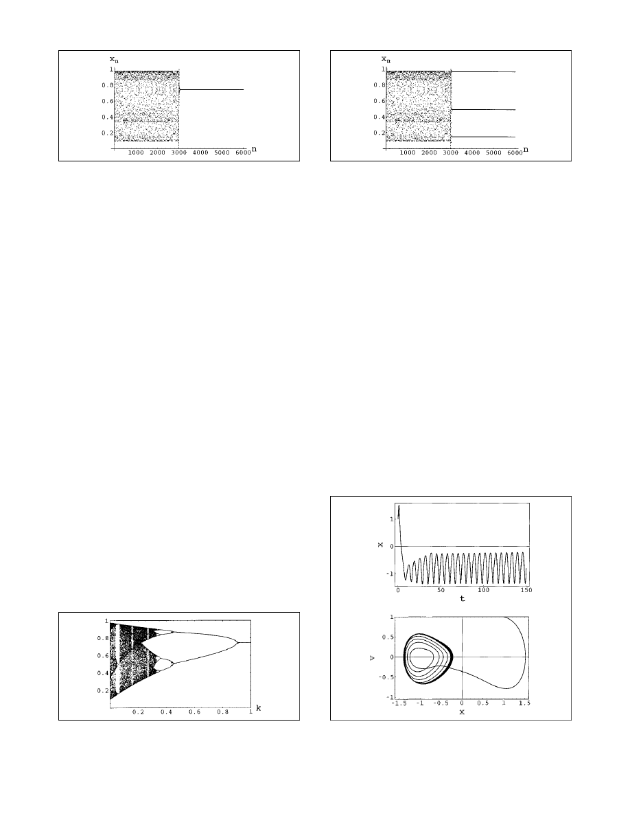
~see Fig. 12!.

upo

5$

0.74359

%

;

FeedbackControl[Logistic[3.9],upo,0.95,0.1,3000,3000]

In this case, the effect of linear-feedback control can

easily be interpreted with the help of the bifurcation dia-
gram of the controlled system as a function of the control
parameter k. Due to the universal character of the bifurca-
tion route for unimodal maps, the controlled map also ex-
hibits a bifurcation route

~shown in Fig. 13!, with the de-

sired period-one point x

50.74359 . . .

LogisticControl[k

–

]

ª

Function[x, 3.9 x (1

2

x)

1

k(x

2

0.74359)];

Bifurcation[LogisticControl[k],

$

k,0,1,250

%

,0.5,150]

This algorithm can be easily extended to deal with

UPOs with arbitrary periods. In this case, the controller

Figure 11. Period-one, -two, and -three UPOs of the Duffing oscillator.

614

COMPUTERS IN PHYSICS, VOL. 12, NO. 6, NOV/DEC 1998

takes the form

v

n

5x

n

2p

mod(n,m)

, where m is the period of

the UPO

$

p

1

, . . . , p

m

%

. For example, in the following we

stabilize a period-3 orbit of the chaotic logistic map

~Fig.

14

!.

PeriodicPoints[Logistic[3.9],x,3]

$

0.132653,0.180986,0.448718,0.578097,0.74359,

0.951213,0.964744

%

upo

5$

0.132653,0.448718,0.964744

%

;

FeedbackControl[Logistic[3.9],upo,0.021,0.1,3000,3000]

A similar idea is applied in Ref. 17 for controlling

nonlinear flows. The Pyragas delayed self-controlling feed-
back method uses a UPO of the flow to build a feedback
controller of the form x

n

5x

n

2p

mod(n,m)

, where m is the

number

of

sampled

points

contained

in

the

UPO

$

p

1

, . . . , p

m

%

. We can use here the algorithms presented in

Sec. II for obtaining UPOs. For instance, consider the cha-
otic Duffing oscillator with f

50.39 shown in Fig. 9. Sup-

pose we want to stabilize one of the period-one UPOs ob-
tained in Sec. II

~Fig. 11!. We can use the

UPO

and

UPOSelect

commands to select the desired unstable orbit,

as we did before:

orb

5

OrbitFlow[Duffing[0.39,1],

$

x,v,z

%

,

$

0,1,0

%

,

$

0,500,0.001

%

];

upos

5

UPO[orb,0.01,500];

upo1

5

First[UPOSelect[upos,

$

124,124

%

]]];

Then, the command

FeedbackFlow

applies the above

feedback-control algorithm to the chaotic Duffing oscillator
in such a way that the system is controlled to the desired
period-one motion

~Fig. 15!.

orb

5

FeedbackFlow[Duffing[0.39,1],

$

x,v,z

%

,

$

1.,1.,1.

%

,

$

0,150,0.05

%

,0.13,125,v,upo1,Show

→

TimeSeries];

ListPlot[First /@ orb]
ListPlot[Drop[#,

2

1]& /@ orb]

In light of these examples we can conclude that feed-

back methods for controlling chaos can be easily imple-
mented, can work automatically after being designed, and
can be interpreted physically. These properties make these
algorithms suitable for many practical applications.

B. Suppressing chaos: Adding pulses to the system variables

The feedback algorithms presented in Sec. III A allow us to
stabilize the chaotic behavior of nonlinear systems by using
some unstable periodic orbit embedded into the chaotic at-
tractor. Although these methods are easy to implement,
they require some knowledge about the system dynamics

~especially in the case of continuous systems!. Chaos-
suppression algorithms allow us to stabilize the system dy-
namics without being concerned with the final stabilized
state. The following example will help us to clarify the
advantages and shortcomings between these two method-
ologies.

Figure 14. Period-three controlled orbit of the logistic map.

Figure 15. Controlled period-one orbit of the chaotic Duffing oscillator
using the Pyragas method.

Figure 12. Period-one controlled orbit of the logistic map. The vertical
dashed line shows the moment at which the chaos-control algorithm starts
being applied.

Figure 13. Bifurcation diagram of the controlled logistic map as a func-
tion of the control parameter k.

COMPUTERS IN PHYSICS, VOL. 12, NO. 6, NOV/DEC 1998

615

As an example of a chaos-suppression algorithm we

consider a recently introduced method that acts on the sys-
tem variables.

7,26

This method does not require any infor-

mation about the system so it is, therefore, applicable even
in situations where there is complete lack of information.
Moreover, in many practical applications, acting on the sys-
tem variables is easier than acting on the system param-
eters. For example, in a chemical reaction it is easy to per-
form changes in the system variables

~by injecting or

removing some components

!, whereas performing changes

in the system parameters may be hard to do.

In the case of maps, the chaos-suppression algorithm

applies a pulse of strength k to the system variables every

Dn iteration steps, either in multiplicative or additive ways,
in the following form:

x

n

→x

n

~11

d

n

Dn

k

!⇔x

n

5 f~r,x

n

21

!~11

d

n

Dn

k

!,

x

n

→x

n

1

d

n

Dn

k

⇔x

n

5 f~r,x

n

21

!1

d

n

Dn

k,

where

d

n

Dn

51, if mod(n,Dn)50, and

d

n

Dn

50, otherwise.

The method can be interpreted by noting that some quantity
of x

n

is injected into or removed from the system every

Dn

iterations, depending on whether k is positive or negative.
The difference between the two alternatives lies in the way
the pulses are introduced. In the multiplicative case, the
pulse depends on the position of the system

~the value of

the variable

! in phase space. The additive method is a sim-

pler alternative that does not require any information about
the system and, hence, is easier to apply in practical situa-
tions.

Using these methods, it is possible to stabilize chaotic

systems by appropriately choosing the strength of the
pulses k and the frequency of application

Dn. The com-

mand

SuppressMap[map, k, dn, x0, a, b]

applies additive or

multiplicative pulses of strength k to the system every dn
iteration steps starting at the initial condition x0. First, a
iterations are performed without applying the method to
show the original system. Then, the method is switched on
the next b steps. For example, the first 3000 iterations in
Fig. 16 show a chaotic orbit of the logistic map. Then, the
control method is switched on and a period-1 orbit is sta-
bilized.

SuppressMap[Logistic[3.9],

2

0.4,1,0.5,3000,3000,

Method

→

Additive]

Note that this orbit is not a true period-one orbit of the

logistic map, but a periodic stable orbit of the auxiliary
system

x

n

11

53.9x

n

~12x

n

!1k.

Then, the performance of the chaos-suppression

method can be qualitatively analyzed with the bifurcation
structure of this auxiliary system as a function of the pa-
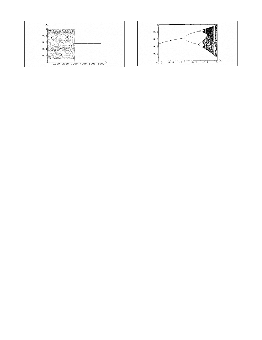
rameter k. Figure 17 shows the bifurcation diagram for the
parameter values in the range k

520.5 to 0. Note that,

when the suppression method is not acting (k

50), the

original chaotic orbit of the system is recovered.

AdditiveControl[k

–

]

ª

Function[x,Logistic[39/10][x]

1

k];

Bifurcation[AdditiveControl[k],

$

k,

2

0.5,0,250

%

,0.5,150]

We can use the commands introduced in Sec. I to

obtain the values of k that stabilize the chaotic system to a
periodic orbit. For instance, if we wish to stabilize the cha-
otic logistic map to a period-one orbit by using the
additive-suppression algorithm we can proceed as follows:

p1

5

PeriodicPoints[AdditiveControl[k],x,1]

H

1

78

~292

A

841

11560k!,

1

78

~291

A

841

11560k!

J

s1

5

Stability[AdditiveControl[k],k,#,x,1]& /@ p1

H

$%

,{{

2

841

1560

,

2

147

520

}}

J

From the above calculations we know that the per-

turbed system has two period-one fixed points. The first one
is never stable and the second one is stable when k is on the
interval

~2~841/1560!, 2~147/520!!.~20.539, 20.283!.

Thus, by choosing a value of k in this range (k

520.4), a

period-1 orbit can be controlled

~see Fig. 16!. Moreover,

we can choose among different values for the period-one
point by substituting k in p1.

The pulses can also be applied in a multiplicative way.

The above analytical study can also be performed in this
case obtaining similar results. For example, by applying
multiplicative pulses of strength k

520.042, the chaotic

logistic map can be switched to a periodic window where a
period-6 orbit is controlled

~Fig. 18!.

SuppressMap[Logistic[3.6],

2

0.042,3,0.5,3000,3000,

Method

→

Multiplicative]

Figure 16. Stabilization of a period-one orbit with the additive chaos-
suppression method.

Figure 17. Bifurcation structure of the perturbed logistic map as a func-
tion of the suppression parameter k.

616

COMPUTERS IN PHYSICS, VOL. 12, NO. 6, NOV/DEC 1998

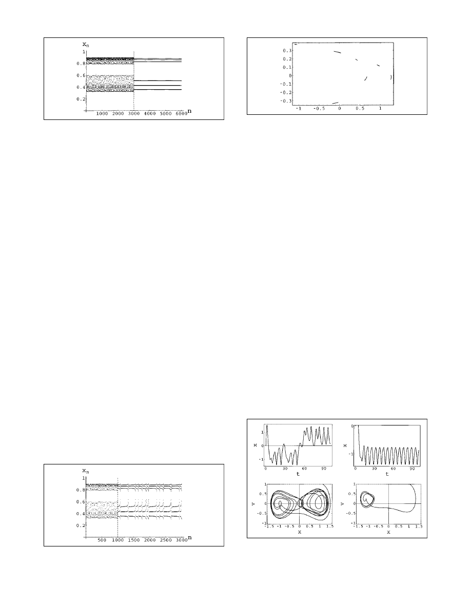
Using the above chaos-control method, we can switch

the chaotic system not only to periodic orbits but also to
any of the unstable behaviors coexisting with the chaotic
system. For example, in the logistic map the transition from
chaos to the period-3 window is done by an intermittent
regimen. This behavior can be stabilized in the chaotic sys-
tem by considering the pulses value k

520.04225, as

shown in Fig. 19.

SuppressMap[Logistic[3.6],

2

0.04225,3,0.5,1000,2000,

Method

→

Multiplicative]

Therefore, when no information about the system is

available, the chaos-control algorithm can be applied by
trying different values for the pulses. However, when the
structure of the system is known, the bifurcation structure
of the controlled system will allow us to predict which
pulse values are needed to control different periodic orbits.
This analysis can also be performed in higher-dimensional
maps.

The

same

algorithm

can

be

applied

to

two-

dimensional maps. In this case, the pulses are introduced in
the system by considering the strength vector k

5(k

1

,k

2

).

For simplicity, we consider k

1

5k

2

, although different or-

bits can be stabilized by applying different pulses to each of
the variables.

As an example of the application of the method, Fig.

20 shows the orbit that results from applying the chaos-
control method with a strength value k

520.00353 to the

He´non map. With this perturbation the system passes
through an interior crisis where the strange attractor sud-
denly shrinks and the system is described in phase space by
seven chaotic segments. In this case, chaos appears from a
crisis route to chaos.

ControlMap2D[Henon[1.282,0.3],

2

0.007,1,

$

0.5,0.5

%

,2000]

Other behaviors can be similarly controlled as, for ex-

ample, the quasiperiodicity route to chaos

~see Ref. 28 for a

more detailed explanation

!.

Introducing pulses into the system variables of con-

tinuous dynamical systems described by differential equa-
tions is not so intuitive as it is in the case of maps. Never-
theless, when using a numerical method to integrate the
differential equations, the continuous orbit of the system is
approximated by a sequence of points sampled at given
time steps. Then, we can take the integration step as an
arbitrary time scale for the perturbations. Thus, the chaos-
suppression algorithm can be described as it is in the dis-
crete case by perturbing the variables every

Dn integration

steps, in both multiplicative and additive ways.

This algorithm is implemented in the command

ControlFlow[flow, x, x0,

$

t0,t1,dt

%

, k]

, which applies pulses to

the system variables during the integration process. Our
goal here is to suppress the chaotic behavior shown in Fig.
9 ( f

50.39). For example, a period-1 orbit can be stabilized

by applying pulses of strength k

520.025 to x ~note that v

and z are auxiliary variables in this example

! every Dn

51 integration steps ~Fig. 21!.

orbs

5

SuppressFlow[Duffing[0.39,1],

$

x,v,z

%

,

$

0,1,0

%

,

$

0,100,0.1

%

,

$

#,0,0

%

,1,Show

→

TimeSeries]& /@

$

0.,

2

0.025

%

;

Show[GraphicsArray[

$

ListPlot[First /@ #]& /@ orbs,
ListPlot[Drop[#,

2

1]& /@ #]& /@ orbs

%

]]

Figure 18. Suppressing chaos with small multiplicative pulses.

Figure 19. Switching from chaos to intermittency in the logistic map.

Figure 20. Suppressing chaos in the He´non map.

Figure 21. Time series and phase-space plot of the original chaotic (left)
and the stabilized (right) orbits of the Duffing oscillator.

COMPUTERS IN PHYSICS, VOL. 12, NO. 6, NOV/DEC 1998

617

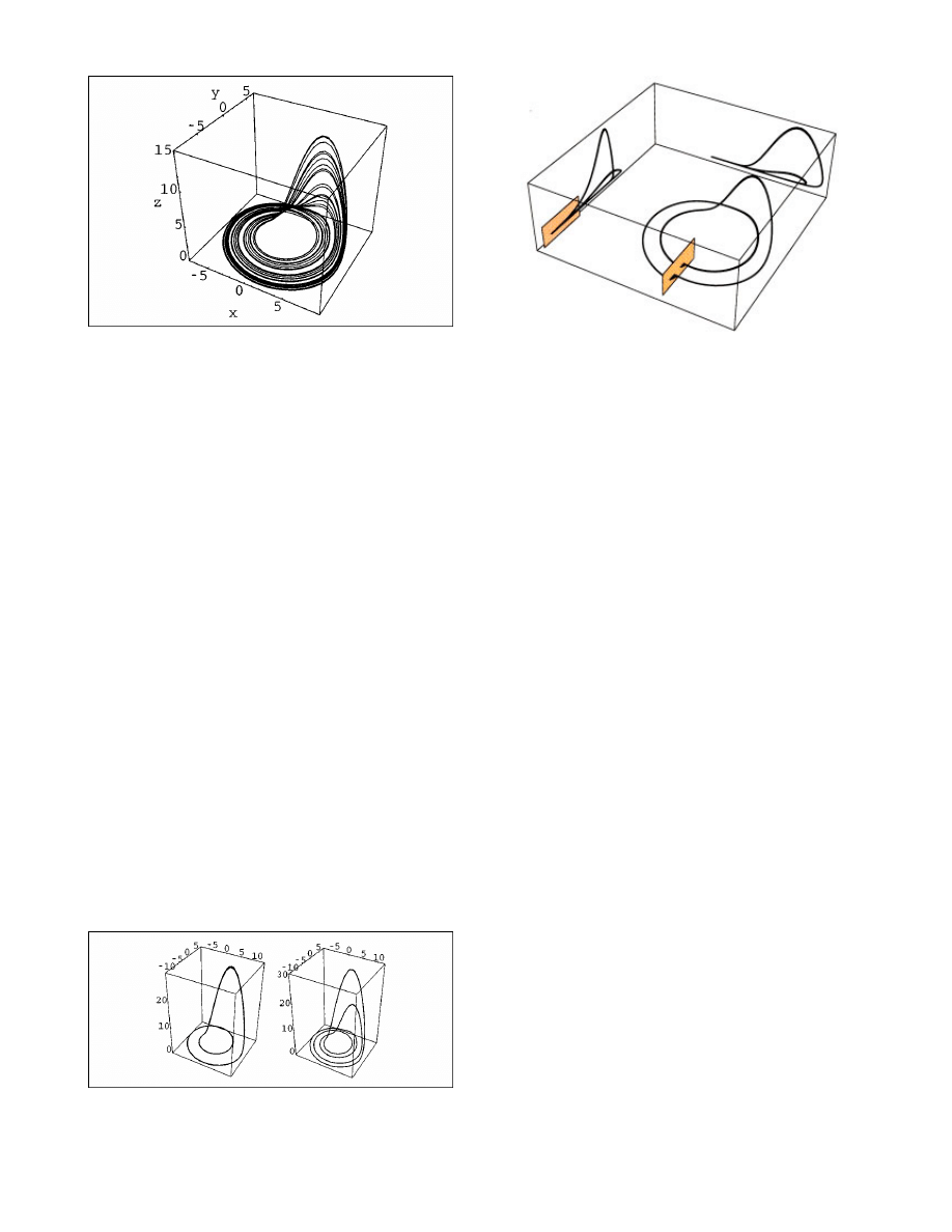
In addition to having been found in the nonlinear os-

cillators described by nonautonomous differential equa-
tions, deterministic chaos has also been found in a great
variety of three-variable autonomous continuous models in
practical applications. An example of this is the Ro¨ssler
model:

29

H

x

8

52y2z,

y

8

5x1ay,

z

8

5b1z~x2c!,

which describes a chemical process. For a

50.2, b50.2

and c

54.6, the Ro¨ssler model exhibits chaos appearing

through a period-doubling bifurcation route

~Fig. 22!.

Rossler

5$2

y

2

z, x

1

0.2

*

y, 0.2

1

z (x

2

4.6)

%

;

OrbitFlow[Rossler,

$

x,y,z

%

,

$

3,3,1

%

,

$

0,150,0.05

%

,

Show

→

Plot3D];

By applying the control method to this system, differ-

ent periodic orbits from the period-doubling route to chaos
can be stabilized. In Fig. 23, period-2 and period-4 orbits
are stabilized by using different pulse strengths:

Show[GraphicsArray

[

SuppressFlow[Rossler,

$

x,y,z

%

,

$

1.,1.,1.

%

,

$

100,150,0.05

%

,

$

#,#,#

%

,10,Show

→

Plot3D]& /@

$2

0.09,

2

0.08

%

]]

The above implementation of the chaos suppression

method for continuous systems uses an arbitrary time scale
for the perturbations. However, it would be better to apply
the pulses in a natural time scale of the system. Such a
natural scale can be given by a Poincare´ section. The per-

turbations can then be introduced in the flow each time the
system crosses the Poincare´ section. This technique is com-
mon within the framework of chaos-control methods

~for

example, it is the key concept in the OGY method

!.

8

Thus,

the continuous system can be controlled by simply control-
ling an associated Poincare´ map, that is, a discrete map.

30

For example, the flow of the Ro¨ssler system is normal to
the plane x

50. This plane can be taken as a Poincare´ sec-

tion of the system. Then, in order to introduce the control
method into a natural time scale of the system, the pulses
should be applied to variables y and z each time the system
crosses the Poincare´ section

~given by the condition x50!.

This section can be specified in Mathematica using the
Boolean condition

x0

,

0 && x1

.

0

, where x0 and x1 are the

x values of two consecutive sampled points, (x0, y 0, z0)
and (x1, y 1, z1), that result from the integration procedure.
The command

SuppressPoincare

implements this algo-

rithm. Figure 24 illustrates its application to the Ro¨ssler
model.

g

5

SuppressPoincare[Rossler,

$

x,y,z

%

,

$

1,1,1

%

,

$

100,150,0.05

%

,

$

0,

2

0.12,

2

0.12

%

,x0

,

0

&&

x1

.

0,

$

x0,y0,z0

%

,

$

x1,y1,z1

%

,

Show

→

Plot3D];

poly

5$

Thickness[0.02],Polygon[

$$

0,

2

3,

2

1

%

,

$

0,

2

3,2

%

,

$

0,

2

10,2

%

,

$

0,

2

10,

2

1

%

,

$

0,

2

3,

2

1

%%

]

%

;

Shadow[Show[

$

g,Graphics3D[poly]

%

,Shading

→

True],

ZShadow

→

False, PlotRange

→

All]

ACKNOWLEDGMENTS

The authors are very grateful to Professor P. Abbott for his
interest in their work and for suggesting that they write this
article. They thank Caja Cantabria and the University of
Cantabria for financial support of this work.

REFERENCES

1. S. Wolfram, The Mathematica 3.0 Book

~Wolfram Media/Cambridge

University Press, Cambridge, 1996

!; Mathematica: A System for Do-

ing Mathematics by Computers

~Addison–Wesley, Reading, MA,

1991

!.

Figure 22. Chaotic attractor of the Ro¨ssler system.

Figure 23. Suppressing chaos in the Ro¨ssler system with pulses of

2

0.09

and

2

0.08, respectively.

Figure 24. Suppressing chaos in the Ro¨ssler system by introducing pulses
in the Poincare´ section (indicated by the rectangle).

618

COMPUTERS IN PHYSICS, VOL. 12, NO. 6, NOV/DEC 1998

2. R. May, Nature

~London! 261, 459 ~1976!.

3. H. G. Schuster, Deterministic Chaos, 2nd ed.

~VCH, 1989!, especially

Chap. 3.

4. E. Ott and M. Spano, Phys. Today 48

~5!, 34 ~1995!.

5. C. Grebogi, E. Ott, and J. A. Yorke, Phys. Rev. A 36, 3522

~1987!.

6. M. He´non, Commun. Math. Phys. 50, 69

~1976!.

7. J. Gu¨e´mez, J. M. Gutie´rrez, A. Iglesias, and M. A. Matı´as, Phys. Lett.

A 190, 429

~1994!.

8. E. Ott, C. Grebogi, and J. A. Yorke, Phys. Rev. Lett. 64, 1196

~1990!.

9. F. C. Moon, Chaotic and Fractal Dynamics

~Wiley, New York,

1992

!.

10. D. P. Lathrop and E. J. Kostelich, Phys. Rev. A 40, 4028

~1989!.

11. W. L. Ditto, N. S. Rauseo, and M. L. Spano, Phys. Rev. Lett. 65, 3211

~1990!.

12. T. Shinbrot, C. Grebogi, E. Ott, and J. A. Yorke, Nature

~London!

363, 411

~1993!.

13. G. Cheng and X. Dong, Int. J. Bifurcation Chaos Appl. Sci. Eng. 3,

1363

~1993!.

14. V. Petrov, V. Gaspar, J. Masere, and K. Showalter, Nature

~London!

361, 240

~1993!.

15. E. R. Hunt, Phys. Rev. Lett. 67, 1953

~1991!.

16. R. Roy, T. W. Murphy, T. D. Maier, Z. Gills, and E. R. Hunt, Phys.

Rev. Lett. 68, 1259

~1992!.

17. K. Pyragas, Phys. Lett. A 170, 421

~1992!.

18. A. W. Hu¨bler, Helv. Phys. Acta 62, 343

~1989!.

19. E. A. Jackson and A. W. Hu¨bler, Physica D 44, 407

~1990!.

20. E. A. Jackson, Phys. Rev. A 44, 4839

~1991!.

21. R. Lima and M. Pettini, Phys. Rev. A 41, 726

~1990!.

22. J. Singer, Y. Z. Wang, and H. H. Bau, Phys. Rev. Lett. 66, 1123

~1991!.

23. Y. Braiman and I. Goldhirsch, Phys. Rev. Lett. 66, 2545

~1991!.

24. R. Chaco´n and J. Dı´az-Bejarano, Phys. Rev. Lett. 71, 3103

~1993!.

25. S. Rajasekar and M. Lakshmanan, Physica D 67, 282

~1993!.

26. M. A. Matı´as and J. Gu¨e´mez, Phys. Rev. Lett. 72, 1455

~1994!.

27. C. K. Chui and G. Chen, Linear Systems and Optimal Control

~Springer, New York, 1989!.

28. A. Iglesias, M. A. Matı´as, J. Gu¨e´mez, and J. M. Gutie´rrez, in Math-

ematics with Vision, edited by V. Keranen and P. Mitic

~Computa-

tional Mechanics, Southampton, 1995

!, pp. 207–214.

29. O. E. Ro¨ssler, Phys. Lett. A 57, 397

~1976!.

30. J. M. Gutie´rrez, A. Iglesias, J. Gu¨e´mez, and M. A. Matı´as, Int. J.

Bifurcation Chaos Appl. Sci. Eng. 6, 1351

~1996!.

COMPUTERS IN PHYSICS, VOL. 12, NO. 6, NOV/DEC 1998

619