Journal of Computer and System Sciences 72 (2006) 1077–1093

www.elsevier.com/locate/jcss

Inoculation strategies for victims of viruses

and the sum-of-squares partition problem

✩

James Aspnes

1

, Kevin Chang

2

, Aleksandr Yampolskiy

∗,3

Department of Computer Science, Yale University, 51 Prospect Street, New Haven, CT 06520-8285, USA

Received 31 October 2004; received in revised form 9 February 2006

Available online 17 April 2006

Abstract

We propose a simple game for modeling containment of the spread of viruses in a graph of n nodes. Each node must choose

to either install anti-virus software at some known cost C, or risk infection and a loss L if a virus that starts at a random initial
point in the graph can reach it without being stopped by some intermediate node. We prove many game theoretic properties of the
model, including an easily applied characterization of Nash equilibria, culminating in our showing that a centralized solution can
give a much better total cost than an equilibrium solution. Though it is NP-hard to compute such a social optimum, we show that
the problem can be reduced to a previously unconsidered combinatorial problem that we call the sum-of-squares partition problem.
Using a greedy algorithm based on sparse cuts, we show that this problem can be approximated to within a factor of O(log

1.5

n)

.

©

2006 Elsevier Inc. All rights reserved.

Keywords: Computer virus model; Economics of security; Security externalities; Price of anarchy; Sum-of-squares partition

1. Introduction

Consider a system in which n machines, each of which may or may not be protected against viruses, are connected

by a network in the form of a graph, and any virus that infects some machine eventually infects all of its unprotected
neighbors. If anti-virus software is available, a natural response would be to protect all the machines—but perhaps
the anti-virus software itself creates costs, both in money and time to purchase and install the software and in reduced
efficiency or usability of the protected machine. Suppose that protecting a machine by installing anti-virus software
costs the owner of the machine C, but that having the machine be infected costs L, which may or may not be greater
than C. If the virus spreads from some initial machine chosen uniformly at random, on which machines does it make
sense to install the anti-virus software?

✩

A preliminary version of this paper appeared in the proceedings of Sixteenth Annual ACM–SIAM Symposium on Discrete Algorithms, January,

2005.

*

Corresponding author.
E-mail addresses: [e-mail] (J. Aspnes), [e-mail] (K. Chang), [e-mail] (A. Yampolskiy).

1

Supported in part by NSF grants CCR-0098078, CNS-0305258, and CNS-0435201.

2

Supported by NSF grant CCR-0331548.

3

Supported by NSF grants CCR-0098078, ANI-0207399, CNS-0305258, and CNS-0435201.

0022-0000/$ – see front matter

© 2006 Elsevier Inc. All rights reserved.

doi:10.1016/j.jcss.2006.02.003

1078

J. Aspnes et al. / Journal of Computer and System Sciences 72 (2006) 1077–1093

The answer will depend on whether we adopt the perspective of the owner of a single machine or of the society as a

whole. When the anti-virus software costs more than the loss from infection, no economically rational machine owner
will install the anti-virus software, every machine will be infected, and the system will incur a social cost of Ln. But
for many graphs, selective inoculation of a few central machines can limit the spread of infection to a small subset of
the graph, greatly reducing the total cost of infection in return for a small investment in anti-virus software. We can
ask how much of an improvement a centralized solution can provide, and how easy it is to find a good centralized
solution.

After discussing some previous work on related problems (in Section 2), we give a complete characterization of

the Nash equilibria for an anti-virus software installation game in which each machine’s owner separately chooses
whether or not to install the software, without regard to the effect on other machines. (This game is defined in Sec-
tion 3.) We show (in Section 4) that finding either the most or least expensive equilibrium is NP-hard, but that some
Nash equilibrium can be computed in O(n

3

)

time and that any population of nodes will quickly converge to a Nash

equilibrium by updating their strategies locally based on the other nodes’ strategies. Unfortunately, the cost of any
such Nash equilibrium may be badly suboptimal; the price of anarchy for this game is Θ(n) in the worst case. This
shows that for many graphs and values of C and L, letting the users choose individually whether or not to inoculate
their machines will give bad results.

We then consider (in Section 5) the possibility of a centralized solution in which a dictator computes and enforces

an optimal inoculation plan. We show that essentially the same argument that shows that extreme Nash equilibria
are hard to find applies to the optimal solution as well. However, we show that the problem of finding an optimal
inoculation plan reduces to a graph partition problem in which we are asked to partition the graph by removing m
nodes; the quality of the partition is measured by the sum of the squares of the sizes of its components. We give
(in Section 6) a polynomial-time approximation algorithm that removes O(log

1.5

n)m

nodes in order to achieve a

partition with quality within O(1) of the optimum. We complement our algorithm with results on the hardness of
approximation of the sum-of-squares partition problem.

Conclusions and open problems appear in Section 7.

2. Related work

In this section, we describe three classes of work related to this paper: virus propagation models, economic models

of investment in security, and game-theoretic models of security. We then discuss some work on graph partitioning
algorithms that are related to the sum-of-squares partition problem we consider in Section 6.

2.1. Virus propagation models

Traditional epidemiological models characterize the viral infection in terms of birth rate and death rate of the

virus [1,2]. Usually, these models assume that an infected individual is equally likely to infect any other individual in
the population; in contrast, computer viruses usually spread via localized interactions. Kephart and White extended the
traditional model by transferring it onto a directed random graph [3]. Later work (e.g., [4–6]) studied virus propagation
over other kinds of graphs, including Internet-like power-law graphs [7–9]. We do not restrict the network topology in
any way and consider a general undirected graph. Our model is in some ways closer to models in percolation theory
(see [10]): an infected node infects all of its unprotected neighbors, spreading infection throughout the graph until it
is blocked by an anti-virus software.

2.2. Economic models of security

Our work is motivated in part by an observation that security technologies exhibit network externalities [11].

Specifically, the benefit obtained by using security technology (anti-virus software in our case) does not accrue only
to the user of the security technology but rather to all users of the network. Aspnes et al. [12] also consider anti-virus
immunization, and proposed studying how to encourage highly connected nodes to use anti-viral techniques.

We assume that costs of installation and infection are known. Alternatively, one could use risk analysis to estimate

the costs and benefits from installing a security technology (see, for example, [13]), or estimate values based on
empirical studies of the costs of security breaches [14,15].

J. Aspnes et al. / Journal of Computer and System Sciences 72 (2006) 1077–1093

1079

2.3. Game-theoretic models of security

Application of game theory to network security has yielded interesting results [16–18]. For example, Bell uses a

simple game to study network reliability. In the game, the router tries to find a least cost path and a network tester
tries to maximize this cost by failing links [19]. Kunreuther and Heal recently introduced the notion of interdependent
security (IDS) games, in which decisions to adopt security technology by one agent affect other agents [20]. Kearns
and Ortiz subsequently extended their paper and gave an algorithm for finding approximate Nash equilibria in this
model [21].

Our work is similar to work on IDS games in certain respects: each agent in both our game and an IDS game

makes a decision whether or not to invest money in a security technology, and this decision affects other agents. The
main differences are that we assume that installing anti-virus software protects against all bad effects of viruses, while
the IDS work concentrates on negative side-effects of security breaches even on protected parties; and we assume a
restricted network topology that contains the spread of viruses, while the IDS work assumes a complete topology.

2.4. Graph partition problems

In Section 6, we describe and provide an approximate solution for a new graph partitioning problem. Previous work

on other forms of graph partitioning includes the approximation algorithm of Leighton and Rao [22] for sparsest cut,
from which the same authors derive a pseudo-approximation algorithm for b-balanced cuts, where each side of the cut
must have size b

|V | or greater. Arora et al. [23] recently improved the approximation ratios of these results. The case

of b

= 1/2 is graph bisection, for which Feige and Krauthgamer [24] give a good approximation algorithm. Even et

al. [25] give O(log n)-ratio pseudo-approximation algorithms for several balanced partitioning problems, including
the ρ-separator problem and the k-balanced partitioning problem.

3. Our model

We represent network topology by an undirected graph G

= (V, E), where V = {0, 1, . . . , n−1} is a set of network

hosts and E

⊆ V ×V is a set of (bidirectional) communication links. Our basic model for installing anti-virus software

is a one-round game with the following features:

Players. Our game has n players corresponding to nodes of the graph. Initially, all nodes are insecure and vulnerable

to infection.

Strategies. We denote the strategy of i by a

i

. Each node i has two possible actions: do nothing and risk being infected

or inoculate itself by installing anti-virus software. Node i’s strategy a

i

is the probability that it inoculates

itself.

Nodes’ choices can be summarized in a strategy profile

a ∈ [0, 1]

n

. If a

i

is 0 or 1, we say that node i

adopts a pure strategy; otherwise, its strategy is mixed. We call nodes that install anti-virus software secure
and denote the set of such nodes by I

a

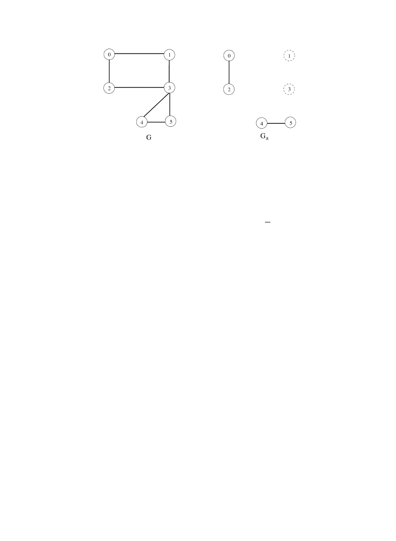
. We associate an attack graph G

a

= G − I

a

with

a. It is essentially

the network graph with secure nodes and their edges removed (see also Fig. 1). Note that both I

a

and G

a

are

random variables unless all strategies are pure.

Attack model. After the nodes made their choices, the adversary picks some node uniformly at random as a starting

point for infection. Infection then propagates through the network graph. Node i gets infected if it has no
anti-virus software installed and if any of its neighbors become infected.

Individual costs. Suppose it costs C to install anti-virus software. If a node is infected, it suffers a loss equal to L.

For simplicity, we assume that both C and L are known and are the same for all nodes; we discuss possible
consequences of removing these assumptions in Section 7.

The cost of a mixed strategy

a ∈ [0, 1]

n

to node i is

cost

i

(

a) = a

i

C

+ (1 − a

i

)L

· p

i

(

a).

Here p

i

(

a) is the probability of node i being infected given the strategy profile a, conditioned on the event

that node i does not install the anti-virus software. It is equal to the probability that some vulnerable node
reachable from i without passing through a secure node is the initial point of infection. For pure strategies,
this is just k

i

/n

, where k

i

is the size of the connected component containing i in the attack graph G

a

.

1080

J. Aspnes et al. / Journal of Computer and System Sciences 72 (2006) 1077–1093

Fig. 1. Sample graph G and its attack graph G

a

for

a = 010100.

Social cost. The total social cost of a strategy profile is the sum of the individual costs. For pure strategies, there is

a simple characterization of the total social cost in terms of the attack graph G

a

. Because each node in the

same component of G

a

has the same chance of infection, the k

i

nodes in the ith component between them

face a loss of k

i

· (Lk

i

/n)

= (L/n)k

2

i

. So the social cost is

cost(

a) =

n

−1

j

=0

cost

j

(

a) =

n

−1

j

=0

a

j

C

+ (1 − a

j

)L

· p

j

(

a) = C|I

a

| +

L

n

l

i

=1

k

2

i

,

where k

1

, k

2

, . . . , k

are the sizes of the components in G

a

.

4. Nash equilibria

We consider first the choices that the nodes will make in the absence of coordination, by examining the Nash

equilibria of the game defined in Section 3. The assumption that the nodes will reach a Nash equilibrium is a very
strong one, as it requires assuming that the nodes are aware of each other’s choices to install or not and that the nodes
can evaluate C (printed on the box for the anti-virus software) and L (which is more problematic). It also assumes
that the nodes can compute a Nash equilibrium in a reasonable amount of time, which is not always possible for some
games. However, we can show that Nash equilibria for our game are easily characterized in terms of the sizes of the
components of the attack graph (Section 4.1), and that a population will converge to some Nash equilibrium quickly
even though finding the best or worst pure equilibrium as measured by total cost is NP-hard (Section 4.2).

We can further imagine that some of the difficulties of limited information could be overcome by considering an

iterated game where nodes pay C to rent the anti-virus software in each round and update their strategies based on
observations of losses to viruses and the strategies of other nodes in previous rounds; though we do not analyze this
multi-round game formally, a simplified version is implicit in our convergence result. We also show that the hardness
of finding the worst-case equilibrium does not prevent obtaining further information about its behavior; for example,
its total cost is non-decreasing as a function of the inoculation cost C (Section 4.3).

Unfortunately, selfish behavior proves to be highly undesirable, because the cost of a Nash equilibrium solution

may be very far from the social optimum. In Section 4.4, we prove that while the price of anarchy, defined as the ratio
of total cost between the worst Nash equilibrium and the social optimum never exceeds n, this bound is tight up to
constant factors for some graphs and choices of C and L.

4.1. Characterization of mixed and pure equilibria

A useful feature of the Nash equilibrium for our game is its simple characterization: there is always a component-

size threshold t

= Cn/L such that each node will install the anti-virus software if it would otherwise end up in

a component of vulnerable nodes with expected size greater than t , and will not install the software if it would
otherwise end up in a component with expected size less than t . When the expected component size equals t , the node
is indifferent between installing and not installing and may adopt a mixed strategy. The threshold arises in a natural

J. Aspnes et al. / Journal of Computer and System Sciences 72 (2006) 1077–1093

1081

way: it is the break-even point at which the cost C of installing the software equals the expected loss L(t/n) of not
installing.

We define

a[i/x] to be the strategy vector that is identical to a, except the ith component a

i

is replaced by x. Note

that attack graph G

a[i/0]

is the attack graph in which player i never installs the anti-virus software.

Theorem 1 (Characterization of mixed equilibria). Suppose S(i) is the expected size of the insecure component that
contains node i of the attack graph G

a[i/0]

(i.e., S(i)

= np

i

(

a)).

Fix C, L. Let the threshold be t

= Cn/L. A strategy profile a is a Nash equilibrium if and only if

(a) for all i such that a

i

= 1, S(i) t;

(b) for all i such that a

i

= 0, S(i) t;

(c) for all i such that 0 < a

i

<

1, S(i)

= t.

Proof. Suppose

a is a Nash equilibrium and consider node i. The expected cost to node i is a

i

C

+ (1 − a

i

)(L/n)S(i)

.

(1) Suppose a

i

= 0. Then node i has expected cost (L/n)S(i). If (L/n)S(i) > C, then i will want find the situation

a

i

= 1 with cost C preferable. Thus, we must have S(i) CL/n = t.

(2) Suppose a

i

= 1. Then node i has expected cost C. If (L/n)S(i) < C, then i would find the situation a

i

= 0 with

expected cost (L/n)S(i) < C preferable. Thus, we must have S(i)

CL/n = t.

(3) Suppose 0 < a

i

<

1. If (L/n)S(i) > C, then i will find the situation a

i

= 1 preferable. If (L/n)S(i) < C, then i

will find the situation a

i

= 0 preferable. Thus, we must have S(i) = CL/n = t.

Thus,

a satisfies condition (a), (b), and (c) above.

Conversely, suppose

a satisfies conditions (a), (b) and (c) of the theorem. Consider node i.

(1) Suppose a

i

= 0. Then node i will have expected cost (L/n)S(i) < C, and thus will not want to switch to a

different a

i

that puts any weight on installing at cost C.

(2) Suppose a

i

= 1. Then node i will have cost C, and thus will not want to switch to a different a

i

that puts any

weight on being insecure at expected cost (L/n)S(i)

C.

(3) Suppose 0 < a

i

<

1. Then node i will have expected cost a

i

C

+ (1 − a

i

)(L/n)S(i)

= C. Switching to any other

strategy will have the same expected cost.

Thus,

a is a Nash equilibrium. 2

A special case of Theorem 1 is the following characterization for pure Nash equilibria. Because nodes in a pure

Nash equilibrium do not make randomized choices, the attack graph is not a random object, but a determined graph.
We have the same threshold conditions as before, but the removal of randomness simplifies the situation.

Corollary 2 (Characterization of pure equilibria). Fix C, L. Let the threshold be t

= Cn/L. A strategy profile a is a

pure Nash equilibrium if and only if

(a) every component in attack graph G

a

has size at most t

;

(b) inserting any secure node j

∈ I

a

and its edges into G

a

yields a component of size at least t .

For example, let C

= 0.5 and L = 1, and consider the graph in Fig. 1. The threshold for this graph is t = Cn/L = 3.

Then Corollary 2 tells us that pure strategy

a = 010100 must be a Nash equilibrium for these C and L.

4.2. Computing pure Nash equilibria

Designing algorithms for finding mixed Nash equilibria or proving hardness results for finding optimized mixed

equilibria would most likely involve estimating or otherwise manipulating the expected value of the sizes of com-
ponents in the attack graph, which is at the very least a non-trivial problem. Furthermore, in the absence of central

1082

J. Aspnes et al. / Journal of Computer and System Sciences 72 (2006) 1077–1093

control, nodes attempting to calculate their best strategy based on a mixed strategy paradigm would possibly run into
similar computational issues.

Thus, we turn our attention to the computation and hardness of pure Nash equilibria. Corollary 2 gives us a powerful

tool with which to reason about pure Nash equilibria. We now show that computing the best or worst pure Nash
equilibria is hard, but that finding some intermediate Nash equilibrium is easy. A consequence of this algorithm is
that the existence of a pure Nash equilibrium is always guaranteed. (The existence of a mixed Nash equilibrium is a
consequence of Nash’s theorem.)

Theorem 3. Both computing the pure Nash equilibrium with lowest cost and computing the pure Nash equilibrium
with highest cost are NP-hard problems.

Proof. We reduce

VERTEX COVER

to the decision problem “Does there exist a pure Nash equilibrium with cost less

than c?” and we reduce

INDEPENDENT DOMINATING SET

to “Does there exist a pure Nash equilibrium with cost

greater than c?”

Fix some graph G

= (V, E), and set C/L = 1.5/n so that t = Cn/L = 1.5, where t is the component size threshold

from Corollary 2. Then from Corollary 2, in any Nash equilibrium the components of the attack graph all have size at
most 1, and any secure node is adjacent to some insecure node (as otherwise it could uninstall its software and be in a
component of size at most 1). It follows that in a Nash equilibrium (a) every vulnerable node is either isolated or has
all neighbors secure, and (b) every secure node has an insecure neighbor.

We now argue that G has a vertex cover of size k if and only if the inoculation game on G with the above settings

of C and L has a Nash equilibrium with k or fewer secure nodes, or equivalently an equilibrium with social cost
Ck

+ (n − k)L/n or less, as each insecure node must be in a component of size 1 and contribute exactly L/n

expected cost. Given a minimal vertex cover V

⊆ V , observe that installing the software on all nodes in V

satisfies

condition (a) because V

is a vertex cover, and (b) because V

is minimal. Conversely, if V

is the set of secure nodes

in a Nash equilibrium, then V

is a vertex cover by condition (a). This concludes the proof that finding a minimum-cost

Nash equilibrium is NP-hard.

For a maximum cost equilibrium, consider the set of insecure vertices. These consist of isolated nodes (which are

already in components of size 1) and nodes that do not install the software because all their neighbors do. Given
an independent dominating set V

⊆ V , installing the software on all nodes except the nodes in V

satisfies condi-

tion (a) because V

is independent and (b) because V

is a dominating set. Conversely, the insecure nodes in any Nash

equilibrium are independent by condition (a) and dominating by condition (b). This shows that G has an independent
dominating set of size k if and only if it has a Nash equilibrium with no more than k insecure nodes, which occurs only
if it has a Nash equilibrium with at least n

−k secure nodes or, equivalently, a cost of at least C(n−k)+(L/n)(k). 2

Theorem 3 says that finding extreme pure equilibria is hard. But what if we just want to converge to some equi-

librium, but we do not care which one? Suppose we implement the process of convergence implied by the Nash
equilibrium: at each step, exactly one participant, whose current strategy is suboptimal given the others’ strategies,
switches (if there are several such participants, we break ties randomly). This is an easy process to implement be-
cause each participant can detect if its strategy is suboptimal using the t

= Cn/L component size threshold from

Corollary 2.

4

But does this process converge to a Nash equilibrium? If it does, how long does it take?

By choosing an appropriate potential function, we can show that this process does indeed converge to a Nash

equilibrium quickly:

Theorem 4. Starting from any pure strategy profile

a, if at each step some participant with a suboptimal strategy

switches its strategy, the system converges to a pure Nash equilibrium in no more than 2n steps.

4

We must assume in this implementation either that the choice to install software or not is reversible, or that each player can observe the other

players’ intended actions and respond accordingly.

J. Aspnes et al. / Journal of Computer and System Sciences 72 (2006) 1077–1093

1083

Proof. Let t

= Cn/L. For any strategy profile a, consider the set S

big

(

a) of “big” components of G

a

of size greater

than t and the set S

small

(

a) of “small” components of G

a

of size less than or equal to t . Define a potential function Φ

by

Φ(

a) =

A

∈S

big

(

a)

|A| −

A

∈S

small

(

a)

|A|.

It is easy to see that

−n Φ(a) n for any a. We will now show that each step of the process reduces Φ by at

least one. There are two main cases:

(1) Some node i switches from insecure to secure. In this case i was previously an element of a component in S

big

of size m > t . This former component becomes one or more new components with total size m

− 1; if all of the

resulting components are big, Φ is reduced by exactly one; otherwise, Φ is reduced by more than one as some
components move from the positive to the negative side of the ledger.

(2) Some node i switches from secure to insecure. In this case the resulting component containing i has m

t

elements, and it replaces one or more old components with total size m

− 1. As both the new component and the

old components are small, the net effect on Φ is to decrease it by one.

If each step reduces Φ by one, the number of steps must be less than the difference between the initial and final

value of Φ, which is at most n

− (−n) = 2n. 2

As a special case, we can start with

a = 1

n

and converge to an equilibrium from above by checking each node once.

Each such test requires computing the size of the component in the attack graph, which takes time O(

|V | + |E|) =

O(n

2

)

using depth-first search; this gives:

Corollary 5. A Nash equilibrium can be computed in time O(n

3

).

It is not hard to see that the 2n in Theorem 4 is close to the best possible bound, although a more careful analysis

might reduce it slightly. A lower bound of n steps is trivial: in a system with C < L/n and no players secure in the
initial strategy profile, it takes n steps for all players to install the anti-virus software. To get closer to 2n, consider
a line with t

=

√

n

− 1/2. Now consider an execution of the process where initially players 1 through n −

√

n

, in

increasing order, install to escape the single overlarge component; but then all players not at positions k

√

n

for some

k

uninstall; this takes 2n

− 2

√

n

steps.

We also have:

Corollary 6. A pure Nash equilibrium always exists.

4.3. Consequences of changes in the inoculation cost

Though Theorem 3 suggests that we cannot hope to characterize the worst pure Nash equilibrium exactly, we can

give a description of how it reacts to changes in the inoculation cost C.

Theorem 7. The cost of the worst pure Nash equilibrium is a non-decreasing function of C when C ranges over
[2L/n, L).

Proof. Fix some price of anti-virus software, C

2L/n so that Cn/L 2. We shall use cost(a; C) to denote the

cost of strategy profile

a when the price is C.

Suppose we increase the price from C to C

= C + ( > 0). We denote the worst-cost Nash equilibrium when

the price is C by

a and the worst-cost equilibrium when the price is C

by

b

.

If the price increment is

L/n, then the threshold (in Theorem 1) increases by at most one; that is, C

n/L

Cn/L + 1. We consider two cases.

1084

J. Aspnes et al. / Journal of Computer and System Sciences 72 (2006) 1077–1093

Case 1.

a is a Nash equilibrium for C

. This case is easy. Because

b

is a worst-cost Nash equilibrium for C

, we have:

cost(

a; C) < cost(a; C

)

cost(b; C

).

Case 2.

a is not a Nash equilibrium for C

. This can happen only if

C

n/L

= Cn/L + 1. Specifically, there must

exist a node w

∈ I

a

such that adding it into attack graph G

a

yields a component of size

Cn/L but not C

n/L

. Let

us denote the sizes of components adjacent to w in G by k

1

, . . . , k

s

.

5

We then have:

s
i

=1

k

i

= Cn/L − 1.

We define a new strategy

a

= a[w/0], which is the same as a except we no longer install anti-virus software on

node w. Moreover,

cost(

a

; C

)

− cost(a; C) =

L

n

Cn/L

2

−

C

+

L

n

s

i

=1

k

2

i

L

n

Cn/L

2

−

s

i

=1

k

i

2

− C

=

L

n

Cn/L

2

−

Cn/L − 1

2

− C.

(1)

Equation (1) is non-negative whenever

2

Cn/L − 1 Cn/L,

which always holds by assumption for all C

2L/n.

We repeat this process until there do not exist any nodes violating Nash equilibrium condition. At each step, the

cost of our new strategy does not decrease. Therefore, if at the end we get a Nash equilibrium

d

, then

cost(

a; C) cost(a; C

)

cost( d; C

)

cost(b; C

).

Because we chose C arbitrarily, our argument holds for all values of .

2

4.4. Price of anarchy

The notion of the price of anarchy was introduced by Koutsoupias and Papadimitriou in [26]. It is defined as the

worst-case ratio between the cost of a Nash equilibrium and the cost of the optimal solution, and is thus a measure of
how far away a Nash equilibrium can be from the social optimum.

6

When the network graph is G and the costs are

C

, L, we use ρ(G, C, L) to denote the price of anarchy.

We show that, in our game, the price of anarchy is quite high, Θ(n). This is a consequence of two simple lemmas.

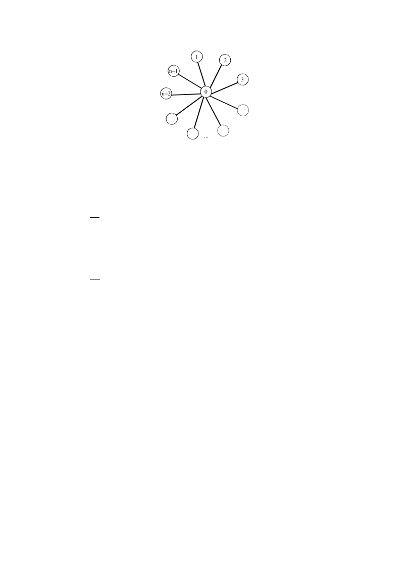
Lemma 8 (Lower bound). Let G be the star graph K

1,n

(see Fig. 2). Let the price of the anti-virus software be

C

= L(n − 1)/n. Then

ρ(G, C, L)

= n/2.

Proof. The given C and L satisfy t

= Cn/L = n − 1. From Corollary 2, it follows that installing anti-virus software

on exactly one node is a Nash equilibrium. If pure Nash strategy

a installs anti-virus software on some node that is

not the center node, the cost will be C

+ L(n − 1)

2

/n

= L(n − 1).

An optimal strategy for the star with the given C and L is

a

∗

= (1, 0, . . . , 0) (i.e., only the center node installs

anti-virus software.) Its cost is C

+ L(n − 1)/n = 2L(n − 1)/n.

The price of anarchy is therefore

L(n

− 1)

2L(n

− 1)/n

=

n

2

.

2

Lemma 9 (Upper bound). Fix any graph G and costs C, L. Then

ρ(G, C, L)

n.

5

We say that a component K

⊆ V is adjacent to node w if ∃v ∈ K s.t. (v, w) ∈ E.

6

Because our game has a random component, the cost is an expected cost.

J. Aspnes et al. / Journal of Computer and System Sciences 72 (2006) 1077–1093

1085

Fig. 2. Star graph G

= K

1,n

used in the proof of the lower bound.

Proof. Let

a

∗

denote the optimum solution.

If C > L, no node in a Nash equilibrium will install anti-virus software. Hence, there is only one Nash equilib-

rium

a = 0

n

, whose cost is Ln. If the optimum solution contains at least one secure node, then cost(

a

∗

)

C > L.

(Otherwise,

a

∗

= 0

n

and ρ(G, C, L)

= 1.) We thus have:

ρ(G, C, L)

Ln

L

= n.

If C

L, then the expected cost of the worst Nash equilibrium a is at most Cn, because the expected cost to

each node is at most C (if the expected cost to a node is greater than C, then it will want to switch to installing the
software with probability 1.) If the optimum solution contains at least one secure node, then cost(

a

∗

)

C. Otherwise,

the optimum solution contains no secure nodes and hence cost(

a

∗

)

L C,

ρ(G, C, L)

Cn

C

= n.

2

5. Optimization

Allowing users to selfishly choose whether or not to install anti-virus software may be grossly inefficient, relative

to the social optimum. An alternative approach to this problem is for a benevolent dictator to attempt to maximize
social welfare by centrally computing a solution and imposing it on all nodes.

Difficulties with this approach arise from the hardness of computing the optimum solution to the inoculation prob-

lem. In the first two sections, we give a characterization of the optimum solution and use it to show that the inoculation
problem is NP-hard.

This suggests computing an approximate solution. We can find in polynomial time a solution with approximation

ratio at most O(log

1.5

n)

; such a solution is substantially better than the Θ(n) ratio derived from the worst Nash

equilibrium.

5.1. Characterization

We have a graph-theoretic characterization of optimum strategies, similar to our characterization of Nash equilibria

in Theorem 1:

Theorem 10. Fix C, L and let t

= Cn/L. If a is an optimum strategy, then every component in attack graph G

a

has

size at most max(1, (t

+ 1)/2).

Proof. Strategy

a partitions G into disjoint components. Pick some component K ⊆ V from the attack graph, where

k

= |K| is at least two. (If we cannot find a component with at least two nodes, then all components in the attack graph

have size one, and the theorem follows.)

If we install the anti-virus software on some node of K, we may get m new components in G

a

, where 0

m

k

− 1. Let us denote the sizes of these new components by k

1

, . . . , k

m

, where

m
i

=1

k

i

= k − 1. Because a is already

1086

J. Aspnes et al. / Journal of Computer and System Sciences 72 (2006) 1077–1093

an optimal strategy, installing the anti-virus software on an extra node cannot improve the total cost. Therefore, we
have:

C

+

L

n

m

i

=1

k

2

i

Lk

2

n

⇔ k

2

−

m

i

=1

k

2

i

t.

(2)

If m

= 0, then Eq. (2) becomes:

k

√

t

(t + 1)/2.

Meanwhile, for m > 0,

k

2

−

m

i

=1

k

2

i

k

2

−

m

i

=1

k

i

2

= k

2

− (k − 1)

2

= 2k − 1.

(3)

Combining Eqs. (2) and (3), we get:

k

(t + 1)/2.

2

Unfortunately, the optimal solution is hard to compute.

Theorem 11. It is NP-hard to compute an optimal strategy.

Proof. The proof is by reduction from

VERTEX COVER

and is similar to the proof of Theorem 3.

2

5.2. Reduction to sum-of-squares partition

Because it is unlikely that we can find an optimal solution, we naturally consider approximation algorithms.
The optimization problem that defines the inoculation problem can be posed as follows: choose the set of secure

nodes I

a

that minimizes the following objective function:

C

|I

a

| +

L

n

V

∈φ(I

a

)

|V |

2

,

where φ(I

a

)

is the set of connected components created by the removal of nodes in I

a

.

For the purposes of our approximation algorithm for the inoculation problem, we assume that we can guess

m

= |I

a

|, the number of secure nodes in an optimum configuration. This assumption is without loss of generality,

because we can run our algorithm on all possible choices of m

= 1, . . . , n and take the best solution.

Thus, a solution to the inoculation problem is reduced to finding a solution to the problem of removing m nodes

from a given graph to minimize the sum of the squares of the sizes of the surviving components. We discuss this
problem in Section 6.

6. Sum-of-squares partitions

In Section 5.2, we encountered the following problem, which we now analyze in more detail.

Sum-of-squares partition problem. Given a graph G

= (V, E), remove a set F ⊆ V of at most m nodes in order to

partition the graph into disconnected components H

1

, . . . , H

l

, such that

i

|H

i

|

2

is minimized.

Although we have arrived at this combinatorial optimization problem through our study of the network security

problem, it may be of independent interest. Note that it is NP-hard by reduction from the inoculation problem. The
edge cut version of the sum-of-squares partition problem is similar, but asks for the removal of m edges, rather than
nodes, to disconnect the graph.

We call an algorithm for the sum-of-squares partition problem an (α, β)-bicriterion approximation algorithm, for

α, β

1, if it outputs a node cut consisting of at most αm nodes that partitions the graph into connected components

J. Aspnes et al. / Journal of Computer and System Sciences 72 (2006) 1077–1093

1087

{H

i

} such that

|H

i

|

2

β · OPT, where OPT is the objective function value of the optimum solution that removes

at most m nodes.

In Section 6.1, we present an algorithm for this problem and in Section 6.2 we prove complementary lower bounds.

Our main result is:

Theorem 12. There exists a polynomial time (O(log

1.5

n), O(

1))-bicriterion approximation algorithm for the sum-of-

squares partition problem.

An immediate consequence of Theorem 12 is the existence of an approximation algorithm for the inoculation

problem:

Corollary 13. If OPT

NS

is the cost of the optimum solution for the inoculation problem, there exists a polynomial-time

approximation algorithm that finds a solution with cost at most O(log

1.5

n)

· OPT

NS

.

Proof. Suppose an optimum solution contains m secure nodes, and the sizes of the insecure node components are
k

1

, . . . , k

p

, so that OPT

NS

= Cm + L/n

i

k

2

i

. Using our approximation algorithm for the sum-of-squares partition

problem, we can find a set of O(log

1.5

n)m

secure nodes such that the sum of the squares of the corresponding insecure

components is at most O(1)

i

k

2

i

. Thus, the cost of the approximate solution is:

O

log

1.5

n

· Cm + O(1) ·

L

n

i

k

2

i

O

log

1.5

n

· Cm + O

log

1.5

n

·

L

n

i

k

2

i

= O

log

1.5

n

· OPT

NS

.

2

6.1. Proof of Theorem 12

Our proof of Theorem 12 is based on the algorithm PartitionGraph given in Fig. 3. It uses known approximation

algorithms for sparse cuts, which usually solve edge cut problems. For our purposes, cuts that involve removing nodes
in order to disconnect the graph are more relevant. Fortunately, the O(

√

log n) approximation algorithm of Arora,

Rao, and Vazirani [23] for finding sparse cuts in graphs with uniform demands can be easily extended to node cuts;
there is a well-known procedure for reducing a node cut algorithm in an undirected graph to an edge cut algorithm
in a directed graph.

7

Since Agarwal et al. [27] extended the algorithm from [23] to find sparse edge cuts in directed

graphs, these results can be extended to node cuts. The following theorem is implicit in the discussion of balanced
node cuts in Leighton and Rao’s paper [22] on multicommodity flows and sparse cuts, with the approximation ratio
updated to reflect the improved algorithms:

Theorem 14. There exists an O(

√

log n)-approximation algorithm for the following problem: given graph G, find a

node cut that partitions the nodes of G into three sets: two sets defining disconnected subgraphs with node sets V

1

and V

2

, and a set of removed nodes R, such that the quantity

(

|V

1

| +

|R|

2

)(

|V

2

| +

|R|

2

)

|R|

(4)

is maximized.

We refer to the quantity in expression (4) as the sparsity of the cut. In the literature, sparsity is usually defined

as the inverse of expression (4), and finding the sparsest cut is a minimization problem. We have presented it as a
maximization problem, since this is more natural for our application.

7

The reduction is as follows: given graph G for which we want a node cut, form directed graph G

∗

with vertex set V

∗

= {v | v ∈ V }∪{v

| v ∈ V }

and edge set E

∗

= {(v, v

)

| v ∈ V } ∪ {(v

, v)

| v ∈ V } ∪ {(v

, u)

| (u, v) ∈ E} ∪ {(u

, v)

| (u, v) ∈ E}. The costs of the {(v, v

)

| v ∈ V } edges are 1,

and all other edges have cost infinity.

1088

J. Aspnes et al. / Journal of Computer and System Sciences 72 (2006) 1077–1093

Input: A graph G and an integer m > 0.
Initialize: G

1

← G. F ← ∅. ← 0.

(1) Use a sparse cut algorithm to find an approximate most cost-effective cut in each connected component of G

.

(2) Let H

1

, . . . , H

k

be the components of G

in which the sparse cut algorithm found a cut that removes at most

(

20c

√

log n)m nodes, where c is the constant from Lemma 15. If no such component exists, then halt and output

the partition of G that results from removing all nodes in set F .

(3) Otherwise, choose the component H

j

from among those considered in step (2) for which the cost-effectiveness is

highest. Let R be the cut that partitions H

j

into disconnected components V

1

and V

2

such that H

j

= V

1

∪ V

2

∪ R.

(4) Set F

← F ∪ R and let G

+1

be the residual graph induced by removing R from G

. If

|F | > (36c log

1.5

n)m

, then

halt and output the partition of G that results from removing all nodes in set F .

(5) Otherwise, set

← + 1 and repeat.

Fig. 3. Algorithm PartitionGraph.

Our algorithm for solving the sum-of-squares partition problem, PartitionGraph (see Fig. 3), achieves the ap-

proximation results claimed in Theorem 12. The general approach of the algorithm is similar to the greedy log n-
approximation algorithm for set cover. A high-level description is that we repeatedly remove the node cut that gives
us the best per-removed-node-benefit, quantified as its cost-effectiveness.

Suppose we have a connected subgraph H with k nodes. If node cut R creates connected components with node sets

V

1

and V

2

, this cut has decreased the objective function value (

size of connected component

2

) by k

2

−|V

1

|

2

−|V

2

|

2

.

We thus define the cost-effectiveness of node cut R by (k

2

− |V

1

|

2

− |V

2

|

2

)/

|R|. The cost-effectiveness of R is equal

to

k

2

− |V

1

|

2

− |V

2

|

2

|R|

=

(

|V

1

| + |V

2

| + |R|)

2

− |V

1

|

2

− |V

2

|

2

|R|

=

|R|

2

+ 2|V

1

||V

2

| + 2|R|(|V

1

| + |V

2

|)

|R|

=

2

|V

1

||V

2

|

|R|

+ |R| + 2

k

− |R|

=

2

|V

1

||V

2

|

|R|

+ 2k − |R|.

We then have the following relationship between finding sparse cuts and cost-effective cuts.

Lemma 15. Let H be a graph with k nodes. If α

∗

is the maximum cost-effectiveness of all node cuts of H , the Arora–

Rao–Vazirani sparse cut algorithm will find a cut with cost-effectiveness at least α

∗

/(c

√

log k), for some constant c.

Proof. The sparsity of a node cut that removes node set R and partitions the remaining nodes of H into connected
components with node sets V

1

and V

2

is given by:

(

|V

1

| +

|R|

2

)(

|V

2

| +

|R|

2

)

|R|

=

|V

1

||V

2

| +

|R|

2

4

+

|R|

2

(

|V

1

| + |V

2

|)

|R|

=

|V

1

||V

2

|

|R|

+

|R|

4

+

1

2

k

− |R|

=

|V

1

||V

2

|

|R|

+

k

2

−

|R|

4

.

We then have the following relations between the cost-effectiveness of a cut, α, and its sparsity, β:

β

=

|V

1

||V

2

|

|R|

+

k

2

−

|R|

4

=

α

2

−

k

2

+

|R|

4

α

4

,

and

α >

2β.

Thus, we know there exists a node cut with sparsity at least α

∗

/

4 (i.e., the cut with the highest cost-effectiveness).

The sparse cut algorithm on H will find a node cut with sparsity at least α

∗

/(c

√

log k), for some constant c. This node

cut will have cost-effectiveness at least 2α

∗

/(c

√

log k).

2

We now give some lemmas that characterize the behavior of the PartitionGraph algorithm.

Lemma 16. PartitionGraph outputs a node cut with at most O(log

1.5

n)m removed nodes.

J. Aspnes et al. / Journal of Computer and System Sciences 72 (2006) 1077–1093

1089

Proof. Since the algorithm halts as soon as we augment the set of marked nodes such that

|F | > (36c log

1.5

n)m

, we

know that at the beginning of each iteration, F contains at most (36c log

1.5

n)m

marked nodes. Since we add at most

(

20c

√

log n)m marked nodes in the final iteration, the total number of marked nodes is at most O(log

1.5

n)m

.

2

Fix an optimum solution for the sum-of-squares partition problem and let F

∗

be the optimum set of m removed

nodes. In the next few proofs, we will denote the order of graph G (i.e., the number of nodes) by

|G| = |V (G)|. We

will also denote an “intersection” of a graph G and a node set V by G

∩ V , which is the set of nodes that G and V

share.

Lemma 17. Suppose after a number of iterations, the graph G

consists of k connected components H

1

, . . . , H

k

, and

let S

=

|H

i

|

2

.

Either S

72 · OPT or there exists a component H

i

such that the Arora–Rao–Vazirani algorithm will find a node

cut in H

i

with at most (20c

√

log n)m removed nodes and cost-effectiveness at least S/(18cm

√

log n) (or possibly

both).

Proof. Assume that S > 72

· OPT. Note that the node cut defined by the set F

∗

∩ G

divides G

into a graph with

objective function value at most OPT. This node cut thus induces a cost decrease of at least S

− S/72 > S/2.

Define F

∗

i

= F

∗

∩ H

i

and m

i

= |F

∗

i

|. Also, let the subgraph induced by removing vertices in F

∗

i

∩ H

i

from H

i

be

composed of connected components H

j

i

for j

= 1, . . . , r

i

(i.e., the optimum set of marked nodes partitions H

i

into

these components). Note that

i

j

|H

j

i

|

2

OPT.

Since the total reduction in our objective function value from removing

i

F

∗

i

from G

is at least S/2 due to our

assumption that S > 2

· OPT, we have:

i

|H

i

|

2

−

j

H

j

i

2

S

2

,

(5)

because the outer summand on the left-hand side of the inequality is the amount the objective function is reduced in
each component.

Let I be the set of indices i for which (

|H

i

|

2

−

r

i

j

=1

|H

j

i

|

2

)/m

i

S/(4m) (i.e., the per-node-benefit is at least

S/(

4m)).

We have two cases. We show that the first case is consistent with the statement of the lemma, whereas the second

case is impossible.

(1) There exists an i

∈ I such that for all j = 1, . . . , r

i

,

|H

j

i

| 1/3|H

i

|. We assume that m

i

<

|H

i

|/50, because

otherwise removing all nodes in H

i

will give us a trivial node cut with cost-effectiveness at least

|H

i

|

2

/(

50m

i

) >

S/(

18cm

√

log n) for sufficiently large n. With this assumption, we know that there exists a set R

⊆ F

∗

i

that defines

a node cut of H

j

i

that creates two connected components, V

1

and V

2

, such that 1/3

|H

i

| |V

1

| and 1/3|H

i

| |V

2

|.

The cost-effectiveness of this cut will be

2

|V

1

||V

2

|

|R|

+ 2|H

i

| − |R|

2

|H

i

|

2

9m

i

2(

|H

i

|

2

−

r

i

j

=1

|H

j

i

|

2

)

9m

i

S

18m

.

Lemma 15 guarantees that the sparse cut algorithm will find a cut in H

i

with cost-effectiveness at least

S/(

18cm

√

log n). The node cut output by the algorithm cannot contain more than 20cm

√

log n nodes. Such a

node cut would have cost-effectiveness at most S/(20cm

√

log n), since any cut in G

can decrease the objective

function value by at most S, which is less than the guaranteed cost-effectiveness of S/(18cm

√

log n).

(2) For each i

∈ I , there exists a j

∗

such that

|H

j

∗

i

| > 1/3|H

i

|. Also, note that OPT >

i

∈I

|H

j

∗

i

|

2

. We prove, by

contradiction, that this case cannot occur. Thus, assume the case does occur.

Claim.

i

∈I

(

|H

i

|

2

−

j

|H

j

i

|

2

)

S/8.

1090

J. Aspnes et al. / Journal of Computer and System Sciences 72 (2006) 1077–1093

Proof. Let ¯

I

be the set of intervals such that (

|H

i

|

2

−

r

i

j

=1

|H

j

i

|

2

)/m

i

S/(4m). Recalling Eq. (5), we have

S/

2

i

∈I

|H

i

|

2

−

j

H

j

i

2

+

i

∈ ¯I

|H

i

|

2

−

j

H

j

i

2

.

Also, we have

i

∈ ¯I

|H

i

|

2

−

j

H

j

i

2

=

i

∈ ¯I

m

i

(

|H

i

|

2

−

j

|H

j

i

|

2

)

m

i

i

∈ ¯I

m

i

S

4m

S

4m

i

∈ ¯I

m

i

S

4

.

Combining these two inequalities proves the claim. We have the inequalities:

OPT >

i

∈I

H

j

∗

i

2

i

∈I

1

9

|H

i

|

2

1

9

·

S

8

,

where we used our claim for the last inequality. Thus, OPT

S/72. This is a contradiction to the assumption we made

at the first line of the proof.

2

We now present the proof of Theorem 12.

Proof. Let a

j

be the number of connected components that comprise the graph G

j

at the beginning of the j th

iteration, and let those connected components be H

j

1

, . . . , H

j

a

j

. Let S

j

=

a

j

i

=1

|H

j

i

|

2

be the value of the objective

function at the beginning of the j th iteration; thus S

0

n

2

is its initial value. Let l be the number of iterations the

algorithm needs to terminate, and S

l

+1

be the objective function’s final value.

We wish to show that after the algorithm terminates, we have reduced the objective function value to S

l

+1

=

O(

1)

· OPT. Let F be the final set of marked nodes removed from G. If the algorithm terminates at step (2) of the lth

iteration because the sparse cut algorithm only found node cuts with more than (20c

√

log n)m removed nodes, then

from Lemma 17 we know that S

l

+1

72 · OPT. Thus, we assume this does not occur. Furthermore, we assume that

S

l

+1

72 · OPT (in order to apply the “either” part of Lemma 17 to all iterations).

In order to reason about the decrease in the objective function value after each iteration, we impute to each node in

F

a per-node-decrease in the objective function value, given by the cost-effectiveness of its node cut. We then show

that the total imputed decrease will decrease the objective function by a factor of O(1)/n

2

, from which the theorem

will follow.

More formally, suppose the set of marked nodes is given by the sequence F

= {f

1

, . . . , f

k

}, where the nodes are

in the order in which they were removed from the graph: nodes removed at an earlier iteration occur earlier in the
sequence. From Lemma 16, we know that k

= |F | = Θ(log

1.5

n)m

.

Let b

j

be the iteration in which f

j

was removed. We impute to f

j

the value δ

j

= cost-effectiveness of cut removed

in iteration b

j

. From Lemma 17, we know that δ

j

S

b

j

/(

18cm

√

log n).

Set T

0

= S

0

and T

i

= T

i

−1

− δ

i

to be the value of the objective function after node f

i

’s per-node-decrease contri-

bution has been accounted for. Note T

k

= S

l

+1

.

Claim. For all i, T

i

T

i

−1

− T

i

−1

/(

18cm

√

log n).

Proof. Proving the claim reduces to proving that δ

i

= T

i

−1

− T

i

T

i

−1

/(

18cm

√

log n). Fix an i. We have two cases.

(1) b

i

= b

i

−1

(i.e., f

i

and f

i

−1

were removed in the same iteration). Then δ

i

S

b

i

/(

18cm

√

log n), but S

b

i

> T

i

,

since S

b

i

is the objective function value at the beginning of iteration b

i

, whereas T

i

is the objective function value

“during” iteration b

i

.

(2) b

i

= b

i

−1

+ 1 (i.e., f

i

was removed in the iteration after f

i

−1

was removed). Then δ

i

S

b

i

/(

18cm

√

log n)

=

T

i

/(

18cm

√

log n), since in this case T

i

is the objective function value at the start of iteration b

i

.

This proves the claim.

2

J. Aspnes et al. / Journal of Computer and System Sciences 72 (2006) 1077–1093

1091

We therefore have T

k

T

0

(

1

−1/(18cm

√

log n))

k

n

2

(

1

−1/(18cm

√

log n))

k

. Since k > 36cm log

1.5

n

, it follows

that S

l

+1

= T

k

= O(1) O(1) · OPT, concluding the proof of Theorem 12. 2

The algorithm given above can be adapted in a straightforward way to yield an algorithm for the edge cut version

of the sum-of-squares partition problem (instead of taking sparse node cuts, take sparse edge cuts), from which an
analog to Theorem 12 may be derived. The above analysis of the node cut algorithm is more complicated than the
corresponding analysis of the edge cut algorithm, since node cuts modify the node set, causing many difficulties.

6.2. Hardness of approximation

In this section, we prove that it is hard to achieve a bicriterion approximation of (α, 1), for some constant α > 1,

by reduction from vertex cover. Hastad [28] proved that it is NP-hard to approximate vertex cover to within a constant
factor of 8/7

−, for any > 0. We show that if we have a graph G with a vertex cover of size m, then a (15/14−, 1)

algorithm for the sum-of-squares partition problem can be used to find a vertex cover in G of size at most (8/7

−2)m.

Theorem 18. It is NP-hard under Cook reduction to approximate the sum-of-squares partition problem to within a
bicriterion factor (15/14

− , 1), for any > 0.

Proof. Suppose graph G

= (V, E), |V | = n, contains a vertex cover C consisting of m nodes. Removing the m

nodes of C and their incident edges will remove all edges from the graph. This will partition the graph into n

− m

disconnected components consisting of 1 node each.

If we consider C as a solution to the sum-of-squares partition problem for removing m nodes, the solution will

have an objective function value of n

− m. Thus, an (α, 1) approximation algorithm for sum-of-squares partition will

remove a set R

⊆ V of nodes, such that |R| αm, in order to achieve an objective function of at most n − m. Let

V

= V \ R be the remaining nodes, and {H

i

} be the connected components in the residual graph.

Let S be the nodes of V

that are contained in connected components of size greater than 1 in the residual graph. It

follows that R

∪ S is a vertex cover of G. We seek to bound the cardinality of R ∪ S.

We first observe that the number of nodes that are contained in connected components of size 1 is

|V

\ S| =

n

− |R| − |S|. Using the fact that if |H

i

| 2, then |H

i

|

2

2|H

i

|, we note that

n

− m

i

|H

i

|

2

i

:

|H

i

|=1

|H

i

|

2

+

i

:

|H

i

|2

|H

i

|

2

n − |R| − |S| + 2|S| n − |R| + |S|.

This implies that

|S| |R| − m αm − m, which implies that |R ∪ S| (2α − 1)m.

Thus, a (15/14

− , 1)-bicriterion approximation algorithm for sum-of-squares partition will find a vertex cover

of size (8/7

− 2)m in G. If OPT

VC

is the cardinality of the optimum vertex cover, then we can search for an

approximately minimum vertex cover by running the algorithm described above for all m

= 1, . . . , n and outputting

the best vertex cover, which will have size at most (8/7

− 2) · OPT

VC

.

2

As mentioned before, sum-of-squares partition is intimately related to the problems of sparsest cut, balanced cut,

and ρ-separator, all with uniform demands (i.e., the nodes all have weight 1). Presently, there are no known hardness
of approximation results for any of these problem; we speculate that techniques for proving hardness of approximation
for both α and β would yield hardness of approximation for some of these fundamental cut problems, which have
proved elusive thus far. We note that Chawla et al. [29] and Khot and Vishnoi [30] have proved super-constant hardness
of approximation results for stronger versions of these problems, specifically sparsest cut and balanced cut with
general demands, assuming the unique games conjecture of Khot [31] (which is a stronger assumption than P

= NP).

7. Conclusions and future research

We have described a simple economic game that represents the difficult problem of choosing on which nodes to

install anti-virus software to contain the spread of computer viruses in a network. The Nash equilibria of this game
have a simple characterization, and we can show that in the worst case, the ratio between the social cost of a Nash
equilibrium and a social optimum can be linear in the number of nodes.

1092

J. Aspnes et al. / Journal of Computer and System Sciences 72 (2006) 1077–1093

Our model makes some very strong simplifying assumptions: every infected node eventually infects all unprotected

neighbors; the costs of installing the anti-virus software and becoming infected are known and equal for all nodes; the
virus imposes no costs on protected nodes; and nodes can observe which of the other nodes intend to install the anti-
virus software and adjust their own strategies in response. None of these assumptions correspond completely to reality,
but we believe that as a first step the resulting model is a reasonable compromise between accuracy and analyzability,
and that the results obtained with the model (especially the characterization of Nash equilibria) are similar to what
one might expect with a more complex model that took into account limited information and learning by individual
nodes. The natural next step is to incorporate more details in the model and see if such changes affect the results; this
might involve both theoretical work to predict the effect of changes and experimental or observational work to study
how real-world decision-makers choose whether or not to deploy specific security mechanisms.

We have also shown how a near-optimal deployment of anti-virus software can be computed by reduction to the

sum-of-squares partition problem, a new variant of classical graph partitioning problems where the goal is to remove
m

vertices so as to minimize the sum of the squares of the sizes of surviving components. Though it is NP-hard to

solve this problem exactly, we give a polynomial-time (O(log

1.5

n), O(

1))-bicriterion approximation algorithm for

sum-of-squares partition, which yields a corresponding approximation algorithm for anti-virus software deployment.
This algorithm may be of use as a network administration tool for choosing how to deploy anti-virus software to min-
imize the combined costs of deployment and infection and as a public-health tool for designing inoculation strategies
for containing outbreaks of highly-infectious diseases when a good approximation to the interaction graph can be
computed but the initial source of contagion is unknown. Whether or not a polynomial-time algorithm with a better
approximation ratio exists remains open.

Acknowledgments

The authors thank Joan Feigenbaum, Hong Jiang, and Yang Richard Yang for many useful discussions.

References

[1] N.T. Bailey, The Mathematical Theory of Infectious Diseases and Its Applications, Hafner Press, 1975.
[2] J.C. Frauenthal, Mathematical Modeling in Epidemiology, Springer-Verlag, New York, 1980.
[3] J.O. Kephart, S.R. White, Directed-graph epidemiological models of computer viruses, in: IEEE Symposium on Security and Privacy, 1991,

pp. 343–361.

[4] J.O. Kephart, D.M. Chess, S.R. White, Computers and epidemiology, in: IEEE Spectrum, 1993, pp. 20–26.
[5] J.O. Kephart, S.R. White, Measuring and modeling computer virus prevalence, in: Proceedings of the IEEE Symposium on Security and

Privacy, 1993, p. 2.

[6] C. Wang, J.C. Knight, M.C. Elder, On computer viral infection and the effect of immunization, in: ACSAC, 2000, pp. 246–256.
[7] R. Pastor-Satorras, A. Vespignani, Epidemics and immunization scale-free networks, in: S. Bornholdt, H. Schuster (Eds.), Handbook of Graphs

and Networks: From the Genome to the Internet, Wiley–VCH, Berlin, 2002, pp. 113–132.

[8] R. Pastor-Satorras, A. Vespignani, Immunization of complex networks, Phys. Rev. Lett. 65 (2002).
[9] C. Zou, D. Towsley, W. Gong, Email virus propagation modeling and analysis, Technical Report CSE-03-04, University of Massachusetts,

Amherst, 2002.

[10] H. Kesten, Percolation Theory for Mathematicians, vol. 2, Birkhäuser, Boston, 1982.
[11] R. Anderson, Why information security is hard—an economic perspective, available at http://www.cl.cam.ac.uk/~rja14/econsec.html, 2001.
[12] J. Aspnes, J. Feigenbaum, M. Mitzenmacher, D. Parkes, Towards better definitions and measures of Internet security, in: Workshop on Large-

Scale Network Security and Deployment Obstacles, 2003.

[13] K. Hoo, How much is enough? A risk-management approach to computer security, Consortium for Research on Information Security Policy

(CRISP), Working Paper, 2000.

[14] K. Campbell, L.A. Gordon, M.P. Loeb, L. Zhou, The economic cost of publicly announced information security breaches: Empirical evidence

from the stock market, J. Comput. Secur. 11 (3) (2003) 431–448.

[15] L.A. Gordon, M.P. Loeb, The economics of information security investment, ACM Trans. Inform. System Secur. (2002) 438–457.
[16] S.N. Hamilton, W.L. Miller, A. Ott, O.S. Saydjari, The role of game theory in information warfare, in: 4th Information Survivability Workshop,

ISW-2001/2002, Vancouver, Canada, 2002.

[17] S.N. Hamilton, W.L. Miller, A. Ott, O.S. Saydjari, Challenges in applying game theory to the domain of information warfare, in: 4th Informa-

tion Survivability Workshop, ISW-2001/2002, Vancouver, Canada, 2002.

[18] P.F. Syverson, A different look at secure distributed computation, in: IEEE Computer Security Foundations Workshop, CSFW 10, IEEE

Comput. Soc. Press, 1997, pp. 109–115.

[19] M.G.H. Bell, The measurement of reliability in stochastic transport networks, in: Proceedings of 2001 Intelligent Transportation Systems,

2001, pp. 1183–1188.

J. Aspnes et al. / Journal of Computer and System Sciences 72 (2006) 1077–1093

1093

[20] H. Kunreuther, G. Heal, Interdependent security, in: Special Issue on Terrorist Risks, J. Risk Uncertainty 26 (2003) 231–249.
[21] M. Kearns, L. Ortiz, Algorithms for interdependent security games, in: S. Thrun, L. Saul, B. Schölkopf (Eds.), Advances in Neural Information

Processing Systems, vol. 16, MIT Press, Cambridge, MA, 2004.

[22] T. Leighton, S. Rao, Multicommodity max-flow min-cut theorems and their use in designing approximation algorithms, J. Assoc. Comput.

Machinery 46 (6) (1999) 787–832.

[23] S. Arora, S. Rao, U. Vazirani, Expander flows, geometric embeddings and graph partitioning, in: Proceedings of the 36th Annual ACM

Symposium on the Theory of Computing, 2004, pp. 222–231.

[24] U. Feige, R. Krauthgamer, A polylogarithmic approximation of the minimum bisection, SIAM J. Comput. 31 (2002) 1090–1118.
[25] G. Even, J. Naor, S. Rao, B. Schieber, Fast approximate graph partitioning algorithms, SIAM J. Comput. 28 (1999) 2187–2214.
[26] E. Koutsoupias, C. Papadimitriou, Worst-case equilibria, in: Proceedings of the 16th Annual Symposium on Theoretical Aspects of Computer

Science, 1999, pp. 403–413.

[27] A. Agarwal, M. Charikar, K. Makarychev, Y. Makarychev, O(

√

log n) approximation algorithms for min uncut, min 2CNF deletion, and

directed cut problems, in: Proceedings of the 37th Annual ACM Symposium on Theory of Computing, 2005, pp. 573–581.

[28] J. Hastad, Some optimal inapproximability results, in: Proceedings of the Twenty-Ninth Annual ACM Symposium on Theory of Computing,

ACM Press, New York, NY, 1997, pp. 1–10.

[29] S. Chawla, R. Krauthgamer, R. Kumar, Y. Rabani, D. Sivakumar, On the hardness of approximating multicut and sparsest-cut, in: IEEE

Conference on Computational Complexity, 2005, pp. 144–153.

[30] S. Khot, N. Vishnoi, The unique games conjecture, integrality gap for cut problems and the embeddability of negative type metrics into l

1

, in:

Proceedings of the 46th IEEE Symposium on Foundations of Computer Science, 2005, pp. 53–62.

[31] S. Khot, On the power of unique 2-prover 1-round games, in: Proceedings of the 34th Annual ACM Symposium on the Theory of Computing,

2002, pp. 767–775.