arXiv:astro-ph/0010634 v1 31 Oct 2000

talk given at the School

Understanding our Universe at the close of 20th Century

25 April 2000 - 6 May 2000

Cargese, France

Supernovae and Cosmology

Monique Signore

?

, Denis Puy

†,‡

?

Laboratoire de Radioastronomie, Observatoire de Paris (France)

†

Paul Scherrer Institut, Villigen (Switzerland)

‡

Institute of Theoretical Physik, University of Zurich (Switzerland)

Abstract

These lecture notes intend to form a short pedagogical introduction to the use of
typical type Ia-Supernovae (hereafter SNIa) as standard candles to determine the
energy density of the universe. Problems of principle for taking SNIa as cosmological
probes are pointed out, and new attempts at solving them are indicated including
the empirical width-luminosity relation (WLR) and its possible explanations.

Finally, the observations of SNIa at high redshift carried out by two major teams

are briefly reviewed and their interpretation as evidence for an accelerating universe
is also rapidly discussed

Key words: Supernovae, Observational cosmology
PACS: 97.60.Bw, 98.80.Es

1

Introduction

A supernova is a very powerful event: a star which suddenly brightens to about
10

9

-10

10

L

. There are two different types of supernovae (see Table 1): SNII

and SNIa, such as:

• SNII are core-collapse induced explosions of short-lived massive stars

(M

?

> 8 M

) which produce more O and Mg relative to F e.

• SNIa are thermonuclear explosions of accreting white-dwarfs in close bina-

ries which produce mostly F e and little O; the exact companions stars of

1

E-mail: [e-mail], [e-mail]

Elsevier Preprint

7 September 2002

white-dwarfs are generally not identified but must be relatively long-lived
stars.

There are also particular supernovae: SNIb and SNIa with most properties
of SNII except their spectra which have no H line (such as SNIa) but they
believed to be core-collapse supernovae (such as SNII).

Type

SNIa

SNII

Hydrogen

no

yes

Optical spectrum

Metal lines

P Cyg lines

deep 6180 ˚

A

Balmer series

Absolute luminosity

∼ 4×10

9

L

∼ 10

9

L

at max. light

small dispersion

large dispersion

standard candles ?

Optical light curve

homogeneous

heteregeneous

UV spectrum

very weak

strong

Radio emission

no detection

strong

slow decay

Location

all galaxies

spirals and irregulars

Stellar population

old

young

Progenitors

WD in binary systems

massive stars

For some time astronomers had focused on all types of supernovae to mea-
sure Hubble’s constant. Now, with the use of Hubble Space Telescope (HST)
observations of Cepheids in the host galaxies of these supernovae, there is a
consensus that H

o

is in the range of 60-70 km s

−1

Mpc

−1

-see Branch (1998)

for a review.
But very recently, two observational groups working independently to use
SNIa as standard candles to measure distance versus redshift presented evi-
dence that the Hubble expansion has been accelerating over time. In effect,
these two independent groups (Perlmutter et al. 1998, Schmidt et al. 1998)
had to develop not only a method of discovering SNIa at high redshift by
careful observations -with large format CCDs, large apertures- and scanning
of plates but they also had to determine if these SNIa could be used as stan-
dard candles. This recent and important progress has been possible because
an empirical relation (Phillips 1993) between the duration of the peak phase
of a SNIa’s light curve and its luminosity (broader is brighter) has been taken
into account by both teams.
This is precisely the work of these two groups that we are trying to present, in

2

an educational manner, in these lessons. In this scope, in section 2, we sum-
marize our current understanding of SNIas: their possible progenitors; some
models of their explosions; observed optical spectra of SNIas, γ-rays from
SNIas, observed optical light curves and finally the empirical width- luminos-
ity relation (WLR) which is also called the Phillips Relation. In section 3,
we give a cosmological background by recalling what is the (Ω

Λ

, Ω

M

)-plane

and the luminosity distance. In section 4, we present the observations of SNIa
at high redshift by the two major teams: the Supernovae Cosmology Project
(SCP) and the High z supernova search team (HZT). In section 5, we discuss
some aspects of their results and finally give a conclusion.

2

On type Ia supernovae

There are spectroscopic and photometric indications that SNIa result from the
thermonuclear explosions of accreting carbon/oxygen white dwarfs (hereafter
WD). However, the progenitor systems of SNIa -their nature, their evolution-
the hydrodynamical models for SNIa- the mass of the WD at ignition, the
physics of the nuclear burnings- are still uncertain.
Moreover, because they are among the brightest optical explosive events in
the universe, and because their light curves and their spectral evolution are
relatively uniform, SNIa have been tentatively used as standard candles. How-
ever variations of light curves and spectra among SNIa have recently been
extensively studied; in particular, the relation between the duration of the
peak phase of their light curves and their luminosities - broader and brighter-
Phillips (1993).
This section briefly summarizes our knowledge of these SNIa properties and
also their controversial issues. However, for more insight into the underly-
ing physics of SNIa and their progenitors, see the various excellent reviews
of Woosley-Weaver (1986), Nomoto et al. (1997), Livio (2000) and most of
the papers of the following proceedings Supernovae (Petscheck, 1990), Ther-
monuclear Supernovae (Ruiz-Lapente et al. 1997); Type Ia Supernovae and
Cosmology (Niemeyer Truran 2000), Cosmic Explosions (Holt & Zhang 2000).

2.1 On the progenitors of SNIa

There are two classes of models proposed as progenitors of SNIa:

i) The Chandrasekhar mass model in which a mass acreting C + O WD grows
in mass up to the critical mass: M

Ia

∼ 1.37 − 1.38 M

-which is near the

Chandrasekhar mass and explodes as a SNIa.
ii) The sub-Chandrasekhar mass model, in which an accreted layer of helium,

3

atop a C + O WD ignites off-center for a WD mass well below the Chan-
drasekhar mass.
The early time spectra of the majority of SNIa are in excellent agreement
with the synthetic spectra of the Chandrasekhar mass models. The spectra of
the sub-Chandrasekhar mass models are too blue to be comparable with the
observations. But let us only give some crude features about the progenitor
evolution.

2.1.1 Chandrasekhar mass models

For the evolution of accreting WD toward the Chandrasekhar mass model, two
scenarii have been proposed: a) a double degenerate (DD) scenario, i.e. the
merging of the C +O WD with a combined mass surpassing the Chandrasekhar
mass M

ch

; b) a single degenerate (SD) scenario, i.e. the accretion of hydrogen

rich matter via mass transfer from a binary companion. The issue of DD versus
SD scenario is still debated. Moreover, some theoretical modeling has indicated
that the merging of WD lead to the accretion-induced collapse rather than a
SNIa explosion.

2.1.2 Sub-Chandrasekhar mass models

In the sub-Chandrasekhar mass model for SNIa, a WD explodes as a SNIa
only when the rate of the mass accretion rate ˙

M is in a certain narrow range.

Moreover, for these models, if ˙

M > ˙

M

crit

, a critical rate, the accreted matter

extends to form a common envelope. However, this difficulty has been recently
overcome by a WD wind model. For the present binary systems which grow
the WD mass to M

Ia

there are two possible systems:

a) a mass-accreting WD and a lobe-filling main sequences star (WD+MS
system).
a) a mass-accreting WD and a lobe-filling less massive red giant star (WD+RG
system).

Let us conclude this subsection by saying that the evolution of the progenitor
is undoubtly the most uncertain part of a fully predictive model of a SNIa
explosion.

2.2 On explosion models

As already noted above, the first important question is about ignition, which
can be formulated as: when and how does the burning start ? We have also

4

seen that there are eventually two candidates:

i) the ignition of

12

C +

12

C, in the core of a WD composed of C + O, is due to

compressive heating from accretion; this is the case of Chandrasekhar models,
for which: M

W D

∼ M

ch

∼ 1.4 M

.

ii) the ignition of He in a shell around a C + O core is followed by the
explosive burning of the C + O core and the helium shell; this is the case of
sub-Chandrasekhar mass models for which 0.7 M

< M

W D

< 1.4 M

.

The second important question is once ignited, does the flame propagate su-
personically by detonation (new fuel heated by shock compression ) ? or sub-
sonically by deflagration (new fuel heated by conduction) ?.
The physics involved in these processes is very complex and relative to the
physics of thermonuclear combustion. In particular, the physics of turbulent
combustion and the possible spontaneous transition to detonation are proba-
bly the most important and least tractable effects. Multidimensional simula-
tions are presently conducted to understand these processes.
Because this work is a pedagogical introduction to the use of SNIa as cosmo-
logical probes, let us only consider Chandrasekhar mass models as standard
SNIa models: they provide a point of convergent evolution for various progen-
itor systems and therefore could offer a natural explanation of the assumed
uniformity of display. Here, we only mention two Chandrasekhar mass models
(groups of Nomoto and Woosley) that can account for the basic features of
the so-called standard SNIa, i.e. : i) an explosion energy of about 10

51

ergs;

ii) the synthesis of a large amount of

56

Ni (∼ 0.6 M

); iii) the production of

substantial amounts of intermediate-mass elements at expansion velocities of
about 10 000 km s

−1

near the maximum brightness of SNIa explosions. All

these features are very important to explain observed optical displays of SNIa:
spectra and light curves.

2.2.1 The carbon deflagration model W7

This model (Nomoto et al. 1984) has been seen for a long time as the standard
explosion model of SNIa. In this model, a subsonic deflagration wave propa-
gates at an average speed of 1/5 of the sound speed from the center to the
expanding outer layers. The explosion synthesis of ∼ 0.58 M

of

56

Ni in the

inner region is ejected with a velocity of 1-2 × 10

4

km s

−1

.

2.2.2 Delayed detonation models

Since 1984, there has been great progress in applying concepts from terrestrial
combustion physics to the SNIa problem. In particular, it has been shown that
the outcome of carbon deflagration depends critically on its flame velocity

5

which is still uncertain. If the flame velocity is much smaller than in W7, the
WD might undergo a pulsating detonation; the deflagration might also induce
a detonation, for instance model DD4 of Woosley & Weaver (1994) or model
WDD2 of Nomoto et al. (1996).
Thus the full details of the combustion are quite uncertain; in particular:
progenitor evolution, ignition densities, effective propagation, speed of the
burning front, type of the burning front (deflagration, detonation, both at
different stages and their transitions).
However, constraints on these still uncertain parameters in models such as
W7, DD4, WDD2 can be provided by comparisons of synthetical spectra and
light curves with observations, by comparisons of predictive nucleosynthesis
with solar isotopic ratio.

2.3 On the observations of SNIa

Here, we only review the observations of SNIa which are relevant for our
cosmological problem which can be formulated by the following question: Can
one consider SNIa as a well-defined class of supernovae in order to use them as
standard candles ? Therefore, we briefly present some of the observed optical
spectra and optical light curves of the so-called SNIa. Moreover, we also give
some considerations on γ-rays from SNIa.

2.3.1 On optical spectra of SNIa

Optical spectra of SNIa are generally homogeneous but one can also observe
some important variations. One recalls that SNIa have not a thick H-rich
envelope so that the elements which are synthesized during their explosions
must be observed in their spectra. Therefore, `a-priori, a comparison between
synthetic spectra and observations can be a powerful diagnostic of dynamics
and nucleosynthesis of SNIa models. Spectra have been calculated for various
models and can be used for comparisons with observations. For instance:

i) Nugent et al. (1997) present agreement between observed spectra of SN
1992A (23 days after the explosion), SN 1994A (20 days after the explosion)
and synthetic spectra of the W7 model for the same epochs after the explo-
sions.
Moreover, the various spectral features can be identified as those of F e, Ca,
S, Si, Mg and O. As already noted above, synthetic spectra for the sub-
Chandrasekhar mass models are less satisfatory.
ii) For heterogeneity Nomoto et al. (1997) present observed optical spectra
of SNIa (SN 1994D, SN 1990N) about one week before maximum brightness
which show different features from those of SN1991T observed at the same

6

epoch. Let us note also that SN1991T is a spectroscopically peculiar SNIa.

2.3.2 On γ-rays from SNIa

SNIa synthesise also radioactive nuclei such as

56

Ni,

57

Ni,

44

T i. The species

56

Ni is certainly the most abundant radioactivity produced in the explosion

of a SNIa. As we will wee below, the amount of

56

Ni (∼ 0.6 M

) is very

important for the physics of the optical light curve of the SNIa. But in fact,
one must consider the following decay chain:

56

Ni

9 days

−→

56

Co

112 days

−→

56

F e + e

+

And, for a certain time after the explosion the hard electromagnetic spectrum
is dominated by γ-rays from the decays of

56

Co. During each decay of

56

Co a

number of γ-rays lines are produced. The average energy is about 3.59 MeV
including 1.02 MeV from e

+

− e

−

annihilations. The most prominent lines are

the 847 keV line and the 1238 keV line. After

56

Co decays, other unstable

nuclei become also important both for the energy budget and for producing
observable hard emissions. One must calculate, for every SNIa model, the
γ-ray light curve, the date, the flux at the maximum of the light curve for
the 847 keV line and 1238 keV line -see for instance many γ-rays papers in
Ruiz-Lapente et al. 1997).

From the observational point of view:

• i) SN 1986G (in NGC 5128) was observed by SMM (Solar Maximum Mis-

sion). An upper limit of: F

847

≤ 2.2 × 10

−4

γ cm

−2

s

−1

was reported leading

to an upper limit of

M

56

(3σ) < 0.4

D

3 Mpc

2

M

.

Later, SN 1986 G was estimated as an under luminous SNIa (Phillips 1993).

• ii) SN1991T (in NGC 4527) was observed by CGRO (Compton Gamma Ray

Observatory) on day 66 after the explosion. A detection by the instrument
COMPTEL/CGRO of the 847 keV line has been reported with a flux of
F

847

= 5.3 ± 2.1 × 10

−5

γ cm

−2

s

−1

. During the same date, no detection,

by the instrument OSSE/CGRO, of the 847 keV line has been reported. A
3σ-upper limit F ≤ 4.5 × 10

−5

γ cm

−2

s

−1

has been given only (see the γ-ray

papers in Ruiz-Lapente et al. 1997 and references therein).
Let us also recall that SN 1991 T was quoted as a peculiar SNIa, from the
point of view of optical spectroscopy (see above 2.3.1).

• iii) An interesting test for the nature of SNIa explosion models has been

found and published just after Cargese 2000, Pinto et al. (2000) present
results of X and γ-ray transport calculations of M

ch

and sub-M

ch

explo-

7

sion models for SNIa and they have shown that X-ray and γ-ray spectral
evolution of both models are very different. In particular, they show that:
· The γ-ray light curves in sub-M

ch

models are much brighter and peak

much earlier than in M

ch

SNIa. The

56

Ni γ-ray line emission (at 847 keV)

from a bright sub-M

ch

explosion at 15 Mpc would be just at the limit for

detection by the ESA satellite INTEGRAL (International Gamma Ray
Astrophysics Laboratory) which will be launched in 2001.

· The presence of surface

56

Ni in sub-M

ch

SNIa would make them very

bright emitters of iron peak K-shell emission visible for several hundred
days after explosion. K-shell emission from a bright sub-M

ch

located near

Virgo would be just above the limit for detection by the XMM observatory.

Anyway, let us only notice that a first true detection of the 847 keV line of
a true typical SNIa by INTEGRAL may help to better understand the SNIa
models and the optical light curves of SNIa (see below 2.3.3).

2.3.3 On optical light curves of SNIa, The Phillips Relation

For a long time, the optical light curve shapes of SNIa were generally supposed
to be homogeneous i.e. all SNIa were identical explosions with identical light
curve shapes and peak luminosities (Woosley & Weaver 1986, see also our
table 1). This was also supported by observations: for instance SN 1980N and
SN 1981D in the galaxy NGC 1316 exhibited almost identical brightness and
identical shapes of their light curves. It was this uniformity in the light curves
of SNIa which had led to their primary use as standard candles in cosmology.
Then, recent work on large samples of SNIa with high quality data has fo-
cused attention on examples of differences within the SNIa class: in particular
there are observed deviations in luminosity at maximum light, in colors, in
light curve widths etc... However, despite all these differences, the discovery of
some regularities in the light curve data has also emerged, in particular, the
Phillips relation: the brightest supernovae have the broadest light curve peaks.
In particular, see the upper plot of figure 2 in section 4. In effect, Phillips (1993)
quantified the photometric differences among a set of nine well-observed SNIa
using the following parameter ∆m

15

(B) which measures the total drop, in B-

magnitudes, from maximum to t = 15 days after B maximum. This Phillips
relation is also called the width luminosity relation (WLR). Finally, it is this
emprical brightness decline relation (WLR) which allows the use of SNIa as
calibrated candles in cosmology -see section 4-
Because SNIa are certainly more complex that can be described as a single-
parameter supernova family, several groups of theorists -experts in supernovae-
have done a lot of work on SNIa in the early times and on their possible evo-
lution until now -see most of the papers written in the proceedings edited by
Niemeyer & Truran (2000) and those edited by Holt & Zhang (2000). But
let us briefly recall how we can explain the present SNIa light curves and the

8

Phillips relation or WLR. See, in particular, Woosley & Weaver (in Petscheck,
1990), Arnett (1996), Nomoto et al. (1997) and more recently Pinto & East-
man (2000a, 2000b, 2000c).
In theoretical models of light curves, the explosion energy goes into the kinetic
energy of expansion E. The light curves are also powered by the radioactive
decay chain:

56

Ni →

56

Co →

56

F e.

The theoretical peaks of the light curve is at about 15-20 days after the ex-
plosion. Their decline is essentially due to the increasing transparency of the
ejecta to γ-rays and to the decreasing input of radioactivity. The light curve
shape depends mainly on the diffusion time:

τ

D

∼

κM

v

esc

c

1

/2

where κ is the opacity, v

esc

∼ (E/M)

1

/2

. Or, in other words, the theoretical

light curve of a SNIa is essentially determined by three effects:

• i) The deposition of energy from radioactive decays.
• ii) The adiabatic conversion of internal energy to kinetic energy of expan-

sion.

• iii) The escape of internal energy as the observed light curve.

A priori. the light curve models of SNIa depends on, at least, four parameters:
1) the total mass M; 2) the explosion energy E; 3) the

56

Ni mass or M

56

; 4)

the opacity κ.
Therefore, the question can be the following one : how these four (or five)
parameters collapse to one for leading to the WLR ? Finally, one must only
mention again the work of Pinto & Eastman (2000c) which shows that:

• 1) The WLR is a consequence of the radiation transport in SNIa.
• 2) The main parameter is the mass of radioactive

56

Ni produced in the

explosion and the rate of change of γ-ray escape.

• 3) The small differences in initial conditions which might arise from evo-

lutionary effects between z ∼ 0 and z ∼ 1 are unlikely to affect the SN
cosmology results.

To conclude this section 2, one can say that although there are uncertainties
in the nature and evolution of SNIa progenitors, in the ignition time and
nature of the burning front, the empirical Phillips relation may be due to the
radiation transport in SNIa and to atomic physics and not to hydrodynamics
of the SNIa explosion (if the results of Pinto & Eastman are confirmed).
Anyway, in section 3, we will recall the cosmological background needed to
use any standard candle for studying the geometry of the Universe -and in
section 4, we will show how cosmologists use the Phillips relation to calibrate
SNIa and use them as calibrated candles.

9

3

Cosmological Background

In order to understand all the cosmological implications of observations of
SNIa at high redshift, one must recall some theoretical background.

3.1 The (Ω

m

,Ω

Λ

)-plane

The cosmological term -i.e. the famous Λ term- was introduced by Einstein
when he applied General Relativity to cosmology:

G

µν

= 8πGT

µν

+ Λg

µν

(1)

where g

µν

is the metric, G

µν

is the Einstein tensor, Λ is the cosmological

constant and T

µν

is the energy- momentum tensor such as ∇

ν

T

µν

= 0.

For a homogeneous and isotropic space-time, g

µν

is the Robertson- Walker

metric:

ds

2

= g

µν

dx

µ

dx

ν

= dt

2

− R

2

h

dr

2

1 − kr

2

+ r

2

(dθ

2

+ sin

2

θ dφ

2

i

(2)

where R(t) is the cosmic scale factor, k is the curvature constant, T

µν

has the

perfect fluid form:

T

µν

= pg

µν

+ (ρ + p)u

µ

u

ν

,

with ρ, p, u

µ

being respectively the energy density, the pressure and the 4-

velocity:

u

µ

=

dx

µ

ds

.

Therefore, the Einstein field equations (1) simplify in:

• The Friedman-Lemaitre equation for the expansion rate H, called the Hub-

ble parameter:

H

2

≡

˙

R
R

2

=

8πGρ

3

+

Λ

3

−

k

R

2

(3)

• An equation for the acceleration:

¨

R
R

= −

4πG

3

(ρ + 3p) +

Λ

3

(4)

where ˙

R = dR/dt and k is the curvature constant which equals respectively

to -1,0,+1 for a universe which is respectively open, flat and closed. Equation
(3) says us that three competing terms drive the expansion: a term of energy

10

(matter and radiation), a term of dark energy or cosmological constant, and
a term of geometry or curvature term.

Remarks: i) if one introduces the equation of state: p = ωρ, let us recall
that ω

R

= 1/3 for the radiation, ω

M

= 0 for the cold matter, ω

Λ

= −1 for

the cosmological constant. ii) Let us notice that one must, a priori, not only
consider a static, uniform vacuum density (or cosmological constant) but also
a dynamical form of evolving , inhomogeneous dark energy (or quintessence);
for this last case: −1 < ω

Q

< 0.

It is convenient to assign symbols to the various fractional constributions of
the energy density at the present epoch such as:

Ω

M

=

8πGρ

o

3H

o

, Ω

Λ

=

Λ

3H

o

and Ω

k

=

k

R

2

o

H

2

o

(5)

where the index o refers to the present epoch. Then equation (3) can be
written:

Ω

m

+ Ω

Λ

+ Ω

k

= 1

(6)

and the astronomer’s cosmological constant problem can be formulated by the
following simple observational question:
Is a non-zero Ω

Λ

required to achieve consistency in equation (6) ?

In comparison with H

o

and Ω

M

, the attempts to measure Ω

Λ

are infrequent and

modest in scope. Moreover signatures of Ω

Λ

are more subtle than signatures

of H

o

and Ω

M

, at least from an observational point of view. Anyway, studying

possible variations in equation (6) having dominant versus negligible Ω

Λ

-term

is quite challenging !
Let us consider now the expansion dynamics in non-zero cosmological constant
models. If:

a ≡

1

1 + z

=

R

R

o

(7)

is the expansion factor relative to the present epoch and if τ = H

o

t is a

dimensionless time variable (i.e. time in units of the measured Hubble time
1/H

o

), the Friedmann equation (3) can be rewritten:

da
dτ

2

= 1 + Ω

M

(

1
a

− 1) + Ω

Λ

(a

2

− 1)

(8)

Ω

M

and Ω

Λ

, here, are constant that parametrize the past (or future) evolution

in terms of quantities of the present epoch.

11

Equivalently, one can also parametrize the evolution with Ω

M

and the decel-

eration parameter q

o

:

q

o

= −

R ¨

R

˙

R

2

o

(9)

which can also be written as:

q

o

=

Ω

M

2

− Ω

Λ

.

(10)

Finally, the expansion dynamics can be given by the system:

˙a

a

2

= Ω

M

(

1
a

)

3

+ (1 − Ω

M

− Ω

Λ

)(

1
a

)

2

+ Ω

Λ

(11)

¨a
a

= Ω

Λ

−

Ω

M

2

(

1
a

)

3

(12)

For different values of (Ω

M

, Ω

Λ

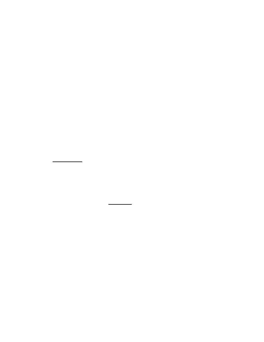
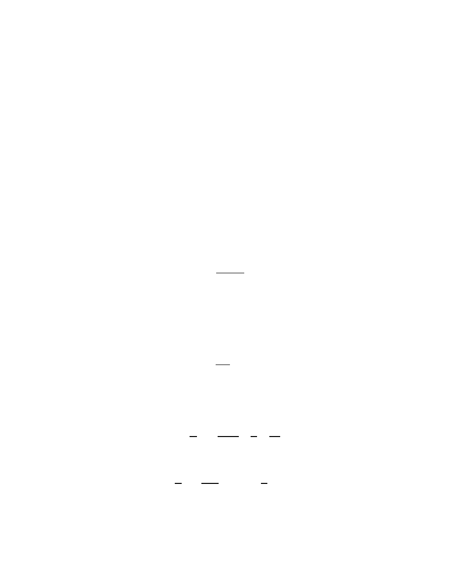
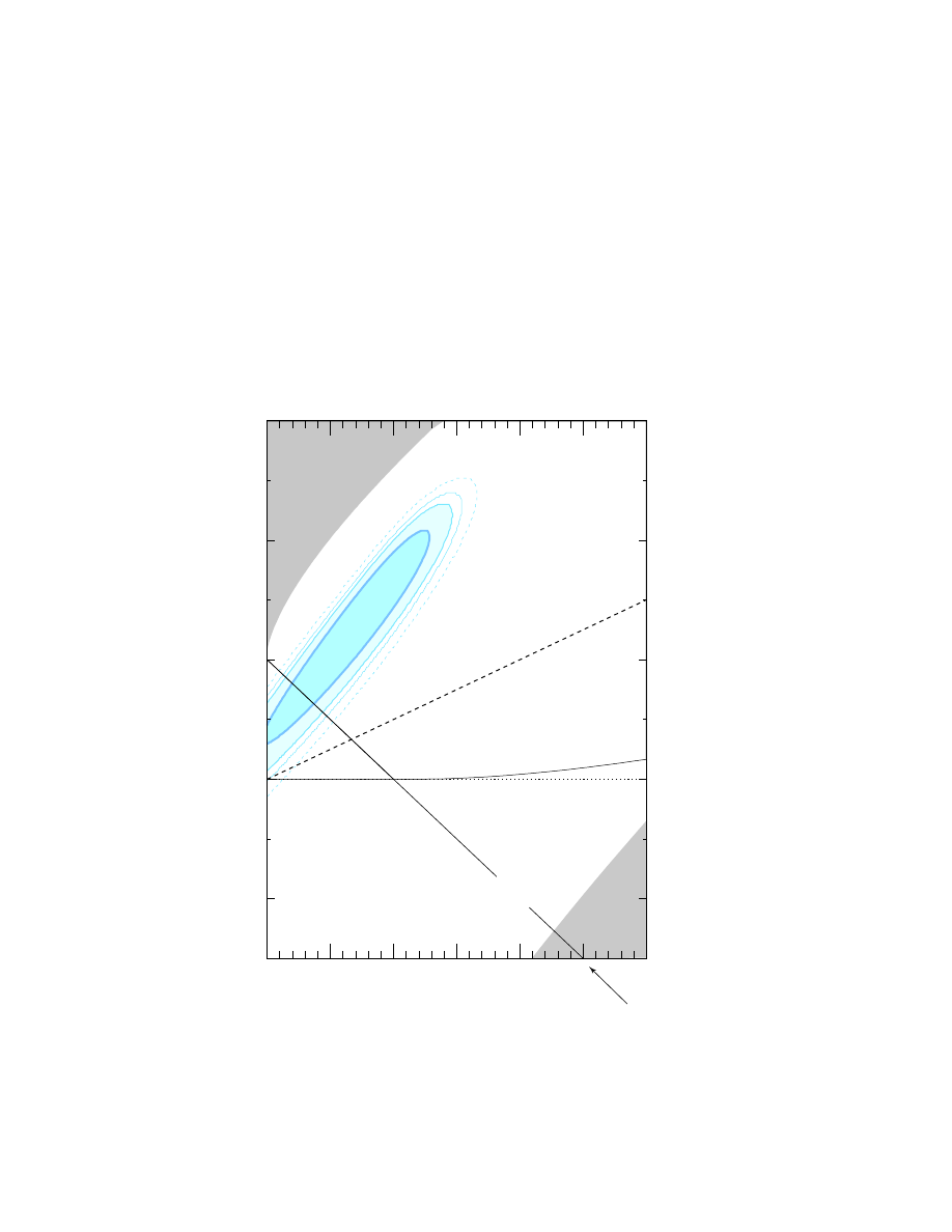
) one gets different expansion histories. Here,

we only give the figure of the (Ω

M

, Ω

Λ

)-plane which displays various possible

regimes -see figure 1 of the (Ω

M

, Ω

Λ

)-plane. Of course, the results of high z-

supernova observations will be first represented by the Hubble diagram, but
their analysis will be given in this (Ω

M

, Ω

Λ

)-plane where it can be confronted

to other major recent cosmological observational results.

Of course, the most direct and theory independent way to measure Λ would
be to actually determine the value of the scale factor a as a function of time.
But, it is very difficult ! However with sufficiently precise information about
the dependence of a distance-measure on z, one will try to disentangle the
effects of matter, cosmological constant and spatial curvature.

3.2 The luminosity distance D

L

The Hubble diagram is a graphic representation of the luminosity distance, i.e.
magnitude, of some class of objects -called standard candles- as a function of
their redshift. Before presenting and discussing the recent results concerning
type Ia-supernovae taken as standard candles, we recall some basic facts.

3.2.1 On the luminosity distance D

L

In cosmology, several different distance measurements are in use. They are
all related by simple z-factors (see for instance Weinberg 1972, Peebles 1993,

12

h
6

Closed Universe

Open Universe

accelerating universe

decelerating universe

q

o

= 0

@

@

R

Flat Universe

expands forever

recollapses

eventually

@

@

R

Λ = 0

Ω

M

Ω

Λ

No

Big Bang

1
|

2
|

0

1

|

2

|

3

0

1

|

2

|

3

-

-

-

-

-

-1

0

1

2

3

-

-

-

-

-

0

1

2

3

Fig. 1. : (Ω

M

,

Ω

Λ

)-plane.

Hoggs 1999). The one which is relevant for our study is the luminosity- dis-
tance:

D

L

=

L

4πF

1

/2

(13)

where L is the intrinsic luminosity of the source and F , the observed flux. For
Friedmann-Lemaitre models, one can show that:

D

L

(z) =

c

H

o

d

L

(z; Ω

M

; Ω

Λ

) = D

H

d

L

(14)

where D

H

≡ c/H

o

is the Hubble distance and d

L

is a known dimensionless

function of z, which depends parametrically on Ω

M

and Ω

Λ

defined by equa-

tions (5). In effect, the luminosity-distance D

L

is related to the transverse-

comoving distance D

m

through:

D

L

= (1 + z)D

m

(15)

13

with:

• D

m

= D

H

Ω

−1

/2

sinh[Ω

1

/2

k

D

c

/D

H

], if Ω

k

> 0

(16)

• D

m

= D

c

= D

H

z

Z

0

dz

0

E(z

0

)

if Ω

k

= 0

(17)

with E(z) = Ω

m

(1 + z)

3

+ Ω

k

(1 + z)

2

+ Ω

Λ

]

1

/2

• D

m

= D

H

Ω

−1

/2

sin[Ω

1

/2

k

D

c

/D

H

], if Ω

k

< 0.

(18)

Therefore, from equations (6) and (14-18) we check that, for different possible
values of Ω

k

:

D

L

= D

L

(z, Ω

M

, Ω

Λ

, H

o

) and d

L

= d

L

(z, Ω

M

, Ω

Λ

)

(19)

3.3 On the magnitude redshift relation

The apparent magnitude m of an object is related to its absolute magnitude
M through the distance modulus by:

m − M = 5log

10

D

L

Mpc

+ 25.

(20)

Therefore, from equation (14-18) and (20) we obtain a relation between the
apparent magnitude m and z with Ω

Λ

and Ω

M

as parameters:

m = 5log

10

d

L

(z, Ω

M

, Ω

Λ

) + M

(21)

Let us only note here that:

• i)M ≡ M − 5log H

o

− 25 is a non-important fit parameter.

• ii) It is the comparison of the theoretical expectation (21) with data which

can lead to constraints on the parameters Ω

M

and Ω

Λ

.

In other words and as we will see, the likelihoods for cosmological parameters
Ω

M

and Ω

Λ

will be determined by minizing the χ

2

statistic between the mea-

sured and predicted distances/magnitudes of SNIa taken as standard candles.

14

4

Observations of SNIa at high redshift

There are two major teams investigating high-z SNIa:

• i) The Supernova Cosmology Project (SCP) which is led by S. Perlmutter

(see S. Perlmutter et al. (1997, 1998, 1999 and references therein).

• ii) The High z-Supernovae Search Team (HZT) which is led by B. Schmidt

(see B. Schmidt et al. (1998 and all references therein).
Both groups have published almost identical results.

In Section (2), we briefly presented SNIa and emphasized that there are large
uncertainties in the theoretical models of these explosive events as well as on
the nature of their progenitors. We have also seen that although they can-
not be considered as perfect standard candles, convincing evidence has been
found for a correlation between light curve shape and luminosity of nearby
SNIa -brighter implies broader- which has been quantified by Phillips (1993).
In this section, we briefly present the cosmological use of SNIa at high red-
shift with: the observations, the results, a discussion of these results and their
cosmological implications.

4.1 The observations

Both groups -the SCP and the HZT- developed a strategy that garantee the
discovery of many SNIa on a certain date. Here, we briefly review the strategy
described by the SCP for its early campaigns.

4.1.1 On the strategy

Just after a new moon, they observed some 50-100 high galactic latitude fields
-each containing about 1000 high-z galaxies- in two nights, at the Cerro-Tololo
4m telescope in Chile with a Tyson and Bernstein’s wide-field-camera. They
returned three weeks later to observe the same fields. About two dozen SNIa
were discovered in the image of the ten thousands of galaxies which were still
brightening since the risetime of a SNIa is longer than 3 weeks. They observed
the supernovae with spectroscopy at maximum light at the Keck-Telescope
and with photometry during the following two months at the Cerro-Tololo
International Observatory (CITO), Isaac Newton Telescope (INT) and -for
the hightest z SNIa- with the Hubble Space Telescope (HST).

15

4.1.2 On spectra

With the Keck (10m-telescope): i) they confirmed the nature of a large num-
ber of candidate supernovae; ii) they searched for peculiarities in the spectra
that might indicate evolution of SNIa with redshift. In effect, as a supernova
brightens and fades, its spectrum changes showing on each day which ele-
ments, in the expanding atmosphere, are passing through the photosphere.
In principle, their spectra must give a constraint on high-z SNIa: they must
show all of the same features on the same day after the explosion as nearby
SNIa; or else, one has evidence that SNIa have evolved between the epoch z
and now.

4.1.3 On light curves

As already noted, in Section 2, nearby SNIa show a relationship between
their peak luminosity and the timescale of their light curve: brighter implies
broader. This correlation, often called Phillips relation or luminosity width
relation (LWR) has been refined and described through several versions of a
one-parameter brightness decline relation: i) ∆m(15) (Hamuy et al. 1996): ii)
multicolor light curve shape (MLCS) (Riess et al. 1996); iii) Stretch parameter
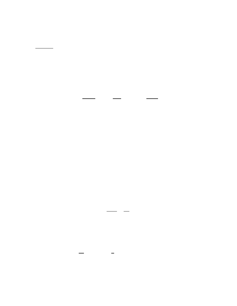
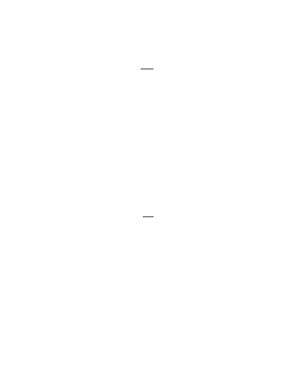
(Perlmutter et al. 1998). Moreover, there exists a simple linear relation between
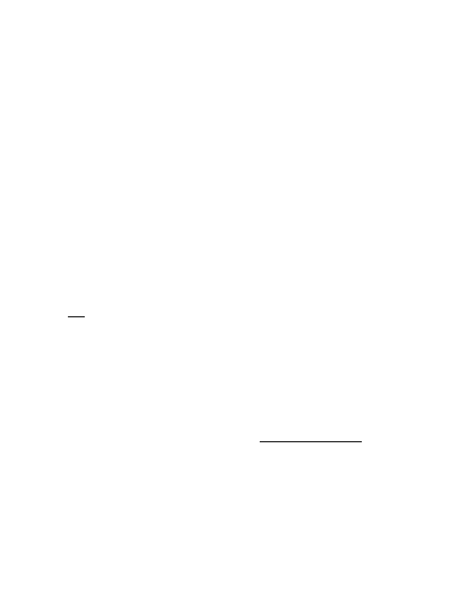
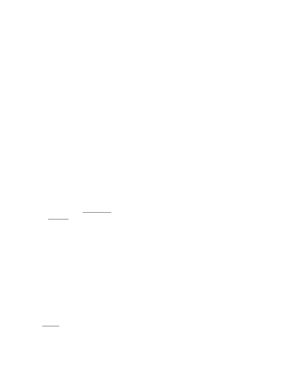
the absolute magnitude and the stretch parameter. Fig. (2) shows how the
stretch correction aligns both the light curve width and the peak magnitude
for the nearby Hamuy supernovae.

4.1.4 On the analysis

One can summarize the three-steps analysis of the 42 high-z SNIa presented
in Perlmutter et al. (1998). For each supernova:

• i) The final image of the host galaxy alone is substracted from the many

images of the given SNIa spanning its light curve.

• ii) Perlmutter et al. (1998) computed a peak-magnitude in the B-band cor-

rected for galaxy extinction and the stretch parameter that stretches the
time axis of a template SNIa (see 4.1.3) to match the observed light curve.

• iii) Then, all of the SN magnitudes -corrected for the stretch-lumisosity

relation- are plotted in the Hubble diagram as a function of their host
galaxy redshift.

16

-20

0

20

40

60

-15

-16

-17

-18

-19

-20

-20

0

20

40

60

-15

-16

-17

-18

-19

-20

B Band

as measured

light-curve timescale

“stretch-factor” corrected

days

M

B

–

5 log(

h/65)

days

M

B

–

5 log(

h/65)

Calan/Tololo SNe Ia

Kim,

et al. (1997)

Fig. 2. : The upper plot shows nearby SNIa light curves which exhibit LWR; the
lower plot shows the nearby SNIa light curves, measured in the upper plot, after
the stretch parameter correction.

4.2 The results and discussion

One must compare the redshift dependence of observed m with the theoretical
expectation given above in Section 3:

m = 5 log d

L

(z, Ω

M

, Ω

Λ

) + M

(22)

17

The effective magnitude versus redshift can be fitted to various cosmologies,
in particular:

• i) to the flat universes (Ω

M

+ Ω

Λ

= 1)

• ii) to the Λ = 0-universes.

4.2.1 On the Hubble diagram

Calan/Tololo
(Hamuy et al,
A.J. 1996)

Supernova
Cosmology
Project

effective

m

B

mag residual

standard deviation

(a)

(b)

(c)

(0.5,0.5)

(0, 0)

( 1, 0 )

(1, 0)

(1.5,–0.5)

(2, 0)

(Ω

Μ,

Ω

Λ

) =

( 0, 1 )

Flat

(0.28, 0.72)

(0.75, 0.25 )

(1, 0)

(0.5, 0.5 )

(0, 0)

(0, 1 )

(Ω

Μ ,

Ω

Λ

) =

Λ = 0

redshift

z

14

16

18

20

22

24

-1.5

-1.0

-0.5

0.0

0.5

1.0

1.5

0.0

0.2

0.4

0.6

0.8

1.0

-6

-4

-2

0

2

4

6

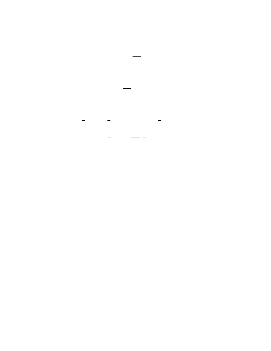
Fig. 3. : From Supernova Cosmology Project (SCP): Hubble diagram.

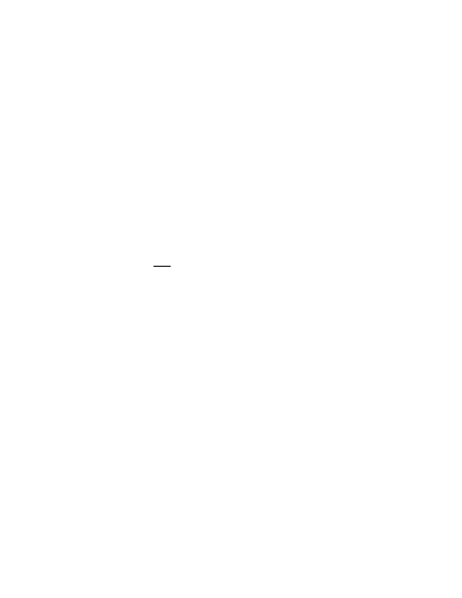
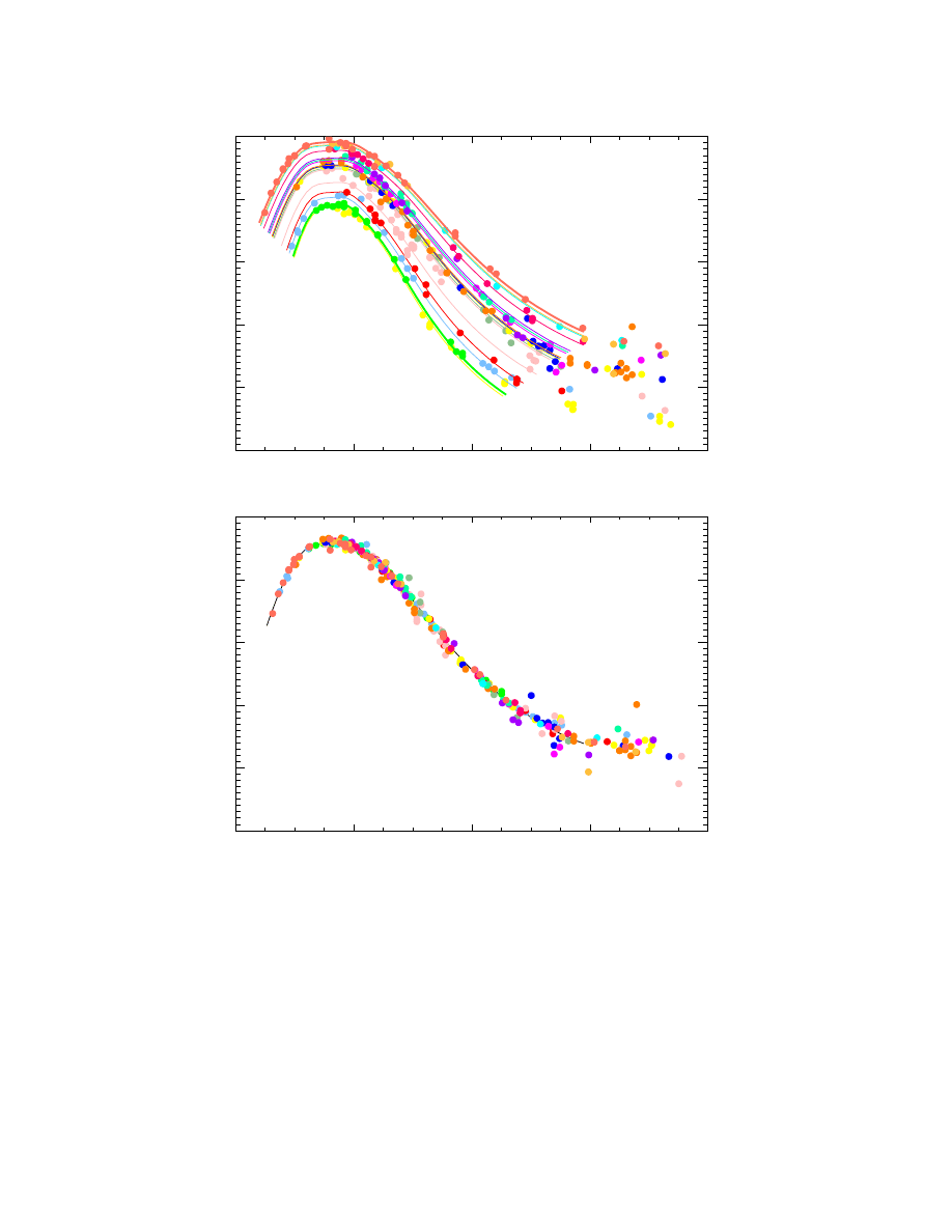
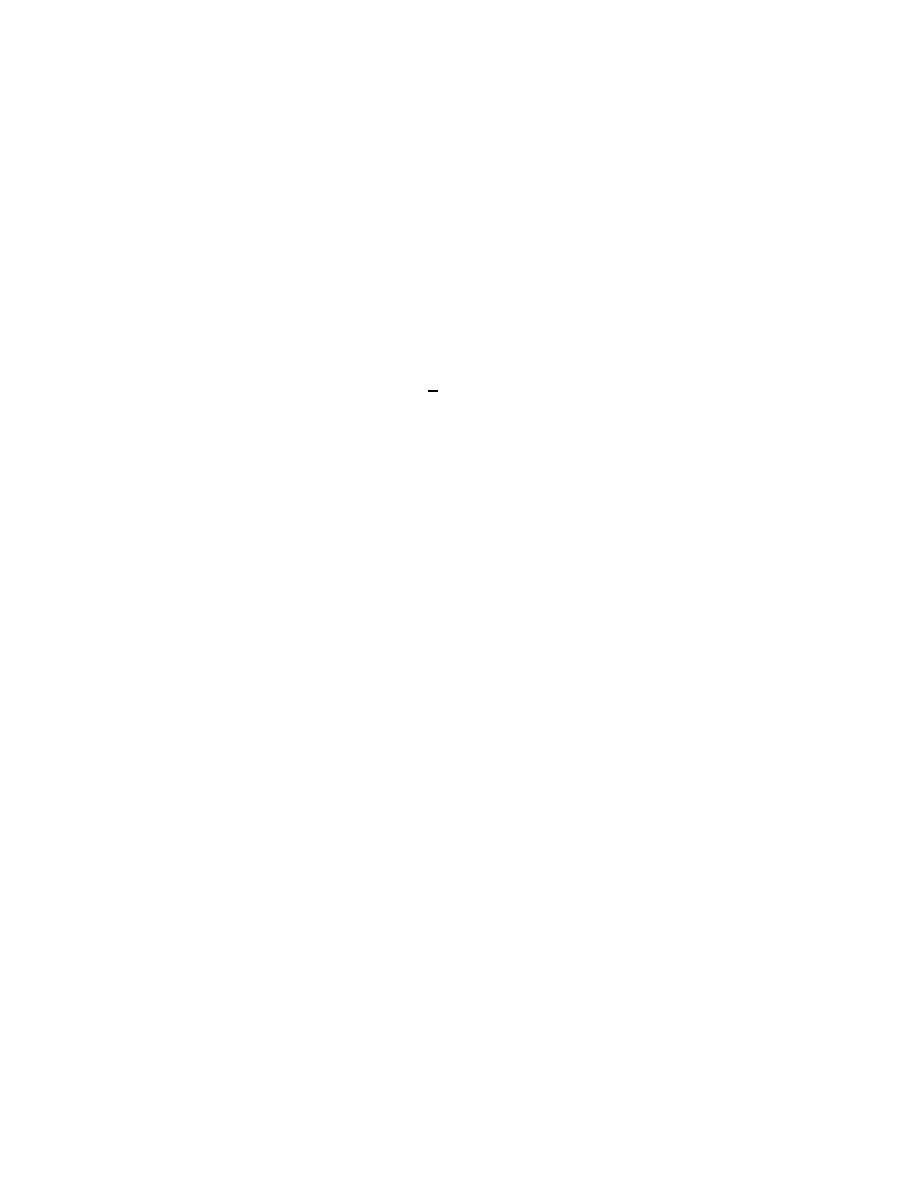
In Fig. (3), one sees the Hubble diagram for 42 high-z SNIa from the SCP and
18 SNIa from the Cal`an-Tololo Supernovae Survey -after correcting both sets
for the LWR (see 4.1.4 above)- on a linear redshift scale to display details at
high z. The solid curves are the theoretical m

ef f
B

(z) for a range of cosmological

models with Λ = 0, (Ω

M

, Ω

Λ

) = (0, 0) on top: (1,0) in middle; (2,0) on bottom.

The dashed curves are for flat cosmological models (Ω

M

+Ω

Λ

= 1): (Ω

M

, Ω

Λ

) =

18

(0, 1) on top; (0.5,0.5) in middle; (1.5,0.5) on bottom. The best fit (Perlmutter
et al. 1998) for a flat Universe (Ω

M

+ Ω

Λ

= 1): Ω

M

∼ 0.28; Ω

Λ

∼ 0.72.

The middle panel of Fig. (3) shows the magnitude residuals between data
and models from the best fit flat cosmology: (Ω

M

, Ω

Λ

) = (0.28, 0.72). The

bottom panel shows the standard deviations. Note that, in their last Hubble
diagram Kim (2000), Perlmutter (2000) extend it beyond z = 1 by estimating
the magnitude of SN1999eq (Albinoni). But, more analysis and more SNIa at
z > 1 are needed.

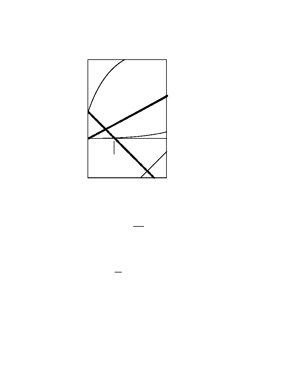
4.2.2 On the (Ω

M

, Ω

Λ

)-plane

No Big Bang

1

2

0

1

2

3

expands foreve

r

-1

0

1

2

3

2

3

closed

open

90%

68%

99%

95%

recollapses eventu

ally

flat

Supernova Cosmology Project
Perlmutter et al.

(1998)

42 Supernovae

mass density

vacuum energy density

(cosmological constant)

decelerating

accelerating

Two groups results agree:
c.f. Riess et al. (1998)

prediction of Guth's

"inflation" theory

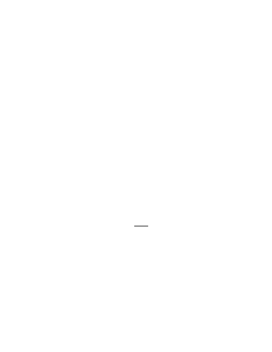
Fig. 4. : From Supernova Cosmology Project (SCP): the (Ω

M

,

Ω

Λ

)-plane.

19

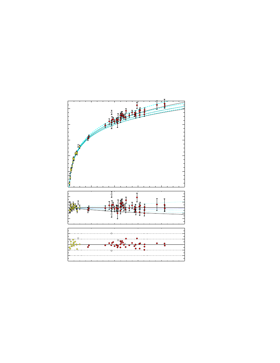
Fig. (4) shows the best fit confidence regions in the (Ω

M

, Ω

Λ

)-plane for the

preliminary analysis of the 42 SNIa fit presented in Perlmutter et al. (1998).
Note that the spatial curvature of the universe -open, flat or closed- is not
deterninative of the future of the universe’s expansion, indicated by the near-
horizontal solid line.
From these figures, one can say that the data are strongly inconsistent with
the Λ = 0, flat universe model. If the simplest inflationary theories are correct
and the universe is spatially flat, then the supernova data imply that there is
a significant positive cosmological constant.
The analysis of Perlmutter et al. (1998) suggested a universe with:

0.8Ω

M

− 0.6Ω

Λ

∼ −0.2 ± 0.1

If one assumes a flat Universe (Ω

M

+ Ω

Λ

= 1), the data imply:

Ω

f lat
M

= 0.28

+0

.09

−0

.08

(1σ

stat

)

+0

.05

−0

.04

(syst.)

More recent data of both groups (SCP and HST) and other independent like-
lihood analysis of the SNIa data provide robust constraints on Ω

M

and Ω

Λ

consistent with those derived by Perlmutter et al. (1998). For a spatially flat
universe, the supernova data require a non-zero cosmological constant at a
high degree of significance (Ω

Λ

≥ 0.5 at 95 % confidence level).

But before interpreting the results of the analysis of the SNIa data, one must
try to discuss the believability of these results.

4.3 Discussion of the results

The current SNIa data set already has statistical uncertainties that are only
a factor of two larger than the identified systematic uncertainties. Here, let
us only list the main indentified sources of systematic uncertainty and only
mention some additional sources of systematic uncertainty (from Perlmutter
2000):

• i) Identified sources of systematic error and their estimated contribution to

the uncertainty of the above measurements:
· Malmquist bias: δM ∼ 0.04
· κ-correction and cross filter calibration: δM < 0.03
· Non-SNIa contamination: δ < 0.05
· Galaxy extinction: δM < 0.04
· Gravitational lensing by clumped mass: δM < 0.06
· Extinction by extragalactic dust:δM ∼ 0.03

• ii) Additional sources of systematic uncertainties:

· Extinction by gray dust

20

· Uncorrected evolution: SNIa behaviour may depend on properties of its

progenitor star or binary-star system. The distribution of these stellar
properties may evolve in a given galaxy and over a set of galaxies.

Let us only notice that the control of statistical and systematic uncertainties
is one of the main goals of the Supernovae Acceleration Probe (SNAP), a 2-m
satellite telescope proposed by Perlmutter (2000)

2

. Such supernova searches,

extended to greater z, can make a much precise determination of the lumi-
nosity distance as a function of z, d

L

(z). Note also that a very optimistic

estimate of the limiting systematic uncertainty of one percent is expected for
such supernovae searches. For a detailed discussion of the present state of all
the systematic uncertainties we refer the reader to the paper of Riess (2000)
and references therein.
Anyway, the believability of the high-z SNIa results turn on the reliability of
SNIa as one-parameter standard candles. The one-parameter is the rate de-
cline of the light curve (the brighter implies the broader) -see subsection 2.3.3
above.
For a while, due to the lack of a good theoretical understanding of the Phillips
relation (what is the physical parameter ?), the supernova experts were not
completely convinced by the high-z SNIa observations and results. After sev-
eral meetings and a lot of theoretical papers -see, in particular, Ruiz-Lapente
et al. (1997) , Niemayer & Truran (2000), Holt & Zhang (2000), and of course
the papers of Pinto & Eastman (2000a, 2000b, 2000c) -the results of (SCP)
and (HZT) appear to supernova experts almost quite convincing... Let us
only recall the conclusion of Wheeler (summary talk of Cosmic Explosions,
December 1999: my personal answer to the question of whether the Universe
is accelerating is probably yes. My answer to the query of do we know for sure
is not yet !.

4.4 Implications of the results. The dark energy

Therefore, if one accepts the high-z SNIa results, the confidence levels in the
(Ω

M

− Ω

Λ

)-plane -which are consistent for both groups (SCP and HZT)- favor

a positive cosmological constant, an accelerating universe and strongly rule
out Ω

Λ

= 0 universes. In other words, the current results of high-z SNIa ob-

servations suggest that the expansion of the Universe is accelerating indicating
the existence of a cosmological constant or dark energy.
There are a number of reviews on the various aspects of the cosmological con-
stant. The classic discussion of the physics of the cosmological constant is by
Weinberg (1989). More recent works are discussed, for instance, by Straumann
(1999), Carroll (2000), Weinberg (2000) and references therein.

2

see http://snap.lbl.gov

21

In particular Weinberg (2000) formulates the two cosmological constant prob-
lems as:

• i) Why the vacuum energy density ρ

v

(or Ω

Λ

) is not very large ?

• ii) Why ρ

v

(or Ω

Λ

) is not only small but also -as high-z SNIa results seem

indicate- of the same order of magnitude as the present mass density of the
universe ?

The challenge for cosmology and for fundamental physics is to determine the
nature of the dark energy. One possibility is that the dark energy consists of
vacuum energy or cosmological constant. In this case -as already noted above
in the remarks of the subsection 3.1- the equation of state of the universe is

ω

Λ

≡

p
ρ

= −1.

An other possibility is quintessence a time-evolving, spatially inhomogeneous
energy component. For this case, the pressure is negative and the equation of
state is a function of z, i.e. ω

Q

(z) is such that:

−1 < ω

Q

(z) < 0.

Let us only notice here that:

• i) these models of dark energy are based on nearly-massless scalar fields

slowly rolling down a potential; most of them are called tracker models of
quintessence for which the scalar field energy density can parallel that of
matter or radiation, at least for part of its history. As Steinhardt said (in the
introductory talk of the Workshop on String Cosmology, Vancouver, August
2000): There are dumb trackers (Steinhardt et al. 1998), smart trackers
(Armandariz-Picon et al. 2000a, 2000b; Bean & Magueijo 2000).

• ii) there are other models of dark energy besides those based on nearly-

massless scalar fields; for instance, models based on networks of tangled
cosmic strings for which the equation of state is: ω

string

= −1/3 or based on

walls for which ω

wall

= −2/3 (Vilenkin 1984, Spergel & Pen 1996, Battye

et al. 1999).

Anyway, a precise measurement of ω today and its time variation could provide
important information about the dynamical properties and the nature of dark
energy. Telescopes may play a larger role than accelerators in determining
the nature of the dark energy. In this context, by observing SNIa at z about
1, SCP and HZT have found strong evidence for dark energy i.e. a smooth
energy component with negative pressure and negative equation of state. For
the future -and as already noted in the subsection 4.2.3- the spatial mission
SNAP is being planned; it is expected that about 1000-2000 SNIa at greater
z (0.1 < z < 1.7) will be detected.
SNAP has also very ambitious goals: it is expected that SNAP will test the

22

nature of the dark energy, will better determine the equation of state of the
universe and its time variation i.e. ω(z). But very recent studies (for instance
Maor et al. 2000) show that the determination of the equation of state of the
Universe by high-z SNIa searches -by using luminosity distance- are strongly
limited.

5

Conclusions

After a brief review of type Ia supernovae properties (Section 2) and of cosmo-
logical background (section 3), we presented the work done by two separate
research teams on observations of high-z SNIa (Section 4) and their interpreta-
tion (Section 5) that the expansion of the Universe is accelerating. If verified,
this will proved to be a remarkable discovery. However, many questions with-
out definitive answers remain.
What are SNIa and SNIa progenitors ?
Are they single or double degenerate stars ?
Do they fit Chandrasekhar or sub-Chandrasekhar mass models at explosion ?
Is the mass of radioactive

56

Ni produced in the explosion really the main pa-

rameter underlying the Phillips relation ?
If so, how important are SNIa evolutionary corrections ?
Can systematic errors be negligible and can they be converted into statistical
errors ?
Can a satellite, like SNAP, provide large homogeneous samples of very dis-
tant SNIa and help determine several key cosmological parameters with an
accuracy exceeding that of planned CMB observations ?

Meanwhile, cosmologists are inclined to believe the SNIa results, because of the
preexisting evidence for dark energy that led to the prediction of accelerated
expansion.

Acknowledgements
The authors gratefully acknowledge Stan Woosley for helpful suggestions. Part
of the work of D.P. has been conducted under the auspices of the Dr Tomalla
Foundation and Swiss National Science Foundation.

References

Armandariz-Picon C. et al. 2000a, astro-ph/0004134
Armandariz-Picon C. et al. 2000b, astro-ph/0006373
Arnett W.D. 1996 in Nucleosynthesis and supernovae, Cambridge Univ. Press

23

Battye R. et al. 1999, astro-ph/9908047
Bean R., Magueijo J. 2000, astro-ph/0007199
Branch D. 1999 ARAA 36, 17
Carroll S. 2000, astro-ph/0004075
Hamuy M. et al. 1996, AJ 112, 2398
Fillipenko A., Riess A. 1999, astro-ph/9905049
Fillipenko A., Riess A. 2000, astro-ph/0008057
Hoggs D. 1999, astro-ph/9905116
Holt S., Zhang W. 2000 in Cosmic Explosions, AIP in press
Kim A. et al. 1997, http://www-supernova.lbl.gov
Kim A. et al. 2000, http://snap.lbl.gov
Livio M. et al. 2000, astro-ph/0005344
Maor I. et al. 2000, astro-ph/0007297
Niemeyer J., Truran J. 2000, in Type Ia Supernovae: Theory and Cosmology
Cambridge Univ. Press
Nomoto K. et al. 1984, ApJ 286, 644
Nomoto K. et al. 1997, astro-/ph/9706007
Nugent et al. 1997 ApJ 485, 812
Peebles J. 1993 in Principles of Physical Cosmology, Princeton Univ. Press
Perlmutter S. et al 1997 ApJ 483, 565
Perlmutter S. et al. 1998 Nature 391, 51
Perlmutter S. et al. 1999 ApJ 517, 365
Perlmutter S. 2000, http://snap.lbl.gov
Petschek A. 1990 in Supernovae, Springer-Verlag
Phillips M. 1993 BAAS 182, 2907
Pinto P., Eastman 2000a ApJ 530, 744
Pinto P., Eastman 2000b ApJ 530, 756
Pinto P., Eastman 2000c, astro-ph/0006171
Pinto P. et al. 2000, astro-ph/0008330
Riess A. et al. 1996, ApJ 473, 588
Riess A. 2000, astro-ph/0005229
Ruiz-Lapente R. et al. 1997 in Thermonuclear supernovae, Kluwer eds
Schmidt B. et al. 1998 ApJ. 507, 46
SNAP (Supernova Acceleration Probe), http://snap.lbl.gov
Spergel D., Pen U. 1997 ApJ 491, L67
Steinhardt P. 1998, astro-ph/9812313
Straumann N. 1999 Eur. J. Phys. 20, 419
Vilenkin A. 1984, Phys. Rev. Lett. 53, 1016
Weinberg S. 1972 in Gravitation and Cosmology, Wiley Eds
Weinberg S. 1989, Rev. Mod. Phys. 61, 1
Weinberg S. 2000, astro-ph/0005265
Wheeler S. 1999, astro-ph/9912403
Woosley S., Weaver T. 1986 ARAA 24, 205
Woosley S., Weaver T. 1994 in Les Houches, session LIV, S. Bludman et al.
Elsevier

24