arXiv:astro-ph/0004075 v2 8 Apr 2000
The Cosmological Constant
Sean M. Carroll
Enrico Fermi Institute and Department of Physics
University of Chicago
5640 S. Ellis Ave.
Chicago, IL 60637 USA
e-mail: carroll@theory.uchicago.edu
http://pancake.uchicago.edu/˜carroll/
Abstract
This is a review of the physics and cosmology of the cosmological constant. Focusing
on recent developments, I present a pedagogical overview of cosmology in the presence
of a cosmological constant, observational constraints on its magnitude, and the physics
of a small (and potentially nonzero) vacuum energy.
Submitted to Living Reviews in Relativity, December 1999
astro-ph/00004075
EFI-2000-13
1
1
Introduction
1.1
Truth and beauty
Science is rarely tidy. We ultimately seek a unified explanatory framework characterized by
elegance and simplicity; along the way, however, our aesthetic impulses must occasionally be
sacrificed to the desire to encompass the largest possible range of phenomena (i.e., to fit the
data). It is often the case that an otherwise compelling theory, in order to be brought into
agreement with observation, requires some apparently unnatural modification. Some such
modifications may eventually be discarded as unnecessary once the phenomena are better
understood; at other times, advances in our theoretical understanding will reveal that a
certain theoretical compromise is only superficially distasteful, when in fact it arises as the
consequence of a beautiful underlying structure.
General relativity is a paradigmatic example of a scientific theory of impressive power
and simplicity. The cosmological constant, meanwhile, is a paradigmatic example of a mod-
ification, originally introduced [1] to help fit the data, which appears at least on the surface
to be superfluous and unattractive. Its original role, to allow static homogeneous solutions
to Einstein’s equations in the presence of matter, turned out to be unnecessary when the
expansion of the universe was discovered [2], and there have been a number of subsequent
episodes in which a nonzero cosmological constant was put forward as an explanation for
a set of observations and later withdrawn when the observational case evaporated. Mean-
while, particle theorists have realized that the cosmological constant can be interpreted as a
measure of the energy density of the vacuum. This energy density is the sum of a number of
apparently unrelated contributions, each of magnitude much larger than the upper limits on
the cosmological constant today; the question of why the observed vacuum energy is so small
in comparison to the scales of particle physics has become a celebrated puzzle, although it is
usually thought to be easier to imagine an unknown mechanism which would set it precisely
to zero than one which would suppress it by just the right amount to yield an observationally
accessible cosmological constant.
This checkered history has led to a certain reluctance to consider further invocations
of a nonzero cosmological constant; however, recent years have provided the best evidence
yet that this elusive quantity does play an important dynamical role in the universe. This
possibility, although still far from a certainty, makes it worthwhile to review the physics
and astrophysics of the cosmological constant (and its modern equivalent, the energy of the
vacuum).
There are a number of other reviews of various aspects of the cosmological constant;
in the present article I will outline the most relevant issues, but not try to be completely
comprehensive, focusing instead on providing a pedagogical introduction and explaining
recent advances. For astrophysical aspects, I did not try to duplicate much of the material
in Carroll, Press and Turner [3], which should be consulted for numerous useful formulae and
a discussion of several kinds of observational tests not covered here. Some earlier discussions
include [4, 5, 6], and subsequent reviews include [7, 8, 9]. The classic discussion of the physics
2
of the cosmological constant is by Weinberg [10], with more recent work discussed by [7, 8].
For introductions to cosmology, see [11, 12, 13].
1.2
Introducing the cosmological constant
Einstein’s original field equations are
R
µν
−
1
2
Rg
µν
= 8πGT
µν
.
(1)
(I use conventions in which c = 1, and will also set ¯
h = 1 in most of the formulae to follow,
but Newton’s constant will be kept explicit.) On very large scales the universe is spatially
homogeneous and isotropic to an excellent approximation, which implies that its metric takes
the Robertson-Walker form
ds
2
=
−dt
2
+ a
2
(t)R
2
0
"
dr
2
1
− kr
2
+ r
2
dΩ
2
#
,
(2)
where dΩ
2
= dθ
2
+ sin
2
θdφ
2
is the metric on a two-sphere. The curvature parameter
k takes on values +1, 0, or
−1 for positively curved, flat, and negatively curved spatial
sections, respectively. The scale factor characterizes the relative size of the spatial sections
as a function of time; we have written it in a normalized form a(t) = R(t)/R
0
, where the
subscript 0 will always refer to a quantity evaluated at the present time. The redshift z
undergone by radiation from a comoving object as it travels to us today is related to the
scale factor at which it was emitted by
a =
1
(1 + z)
.
(3)
The energy-momentum sources may be modeled as a perfect fluid, specified by an energy
density ρ and isotropic pressure p in its rest frame. The energy-momentum tensor of such a
fluid is
T
µν
= (ρ + p)U
µ
U
ν
+ pg
µν
,
(4)
where U
µ
is the fluid four-velocity. To obtain a Robertson-Walker solution to Einstein’s
equations, the rest frame of the fluid must be that of a comoving observer in the metric (2);
in that case, Einstein’s equations reduce to the two Friedmann equations
H
2
≡
˙a
a
2
=
8πG
3
ρ
−
k
a
2
R
2
0
,
(5)
where we have introduced the Hubble parameter H
≡ ˙a/a, and
¨
a
a
=
−
4πG
3
(ρ + 3p) .
(6)
3
Einstein was interested in finding static ( ˙a = 0) solutions, both due to his hope that
general relativity would embody Mach’s principle that matter determines inertia, and simply
to account for the astronomical data as they were understood at the time.
A static universe
with a positive energy density is compatible with (5) if the spatial curvature is positive
(k = +1) and the density is appropriately tuned; however, (6) implies that ¨
a will never
vanish in such a spacetime if the pressure p is also nonnegative (which is true for most
forms of matter, and certainly for ordinary sources such as stars and gas). Einstein therefore
proposed a modification of his equations, to
R
µν
−
1
2
Rg
µν
+ Λg
µν
= 8πGT
µν
,
(7)
where Λ is a new free parameter, the cosmological constant. Indeed, the left-hand side
of (7) is the most general local, coordinate-invariant, divergenceless, symmetric, two-index
tensor we can construct solely from the metric and its first and second derivatives. With
this modification, the Friedmann equations become
H
2
=
8πG
3
ρ +
Λ
3
−
k
a
2
R
2
0
.
(8)
and
¨
a
a
=
−
4πG
3
(ρ + 3p) +
Λ
3
.
(9)
These equations admit a static solution with positive spatial curvature and all the parameters
ρ, p, and Λ nonnegative. This solution is called the “Einstein static universe.”
The discovery by Hubble that the universe is expanding eliminated the empirical need
for a static world model (although the Einstein static universe continues to thrive in the
toolboxes of theorists, as a crucial step in the construction of conformal diagrams). It has
also been criticized on the grounds that any small deviation from a perfect balance between
the terms in (9) will rapidly grow into a runaway departure from the static solution.
Pandora’s box, however, is not so easily closed. The disappearance of the original mo-
tivation for introducing the cosmological constant did not change its status as a legitimate
addition to the gravitational field equations, or as a parameter to be constrained by obser-
vation. The only way to purge Λ from cosmological discourse would be to measure all of the
other terms in (8) to sufficient precision to be able to conclude that the Λ/3 term is negligibly
small in comparison, a feat which has to date been out of reach. As discussed below, there
is better reason than ever before to believe that Λ is actually nonzero, and Einstein may not
have blundered after all.
1.3
Vacuum energy
The cosmological constant Λ is a dimensionful parameter with units of (length)
−2
. From the
point of view of classical general relativity, there is no preferred choice for what the length
1
This account gives short shrift to the details of what actually happened; for historical background see
4
scale defined by Λ might be. Particle physics, however, brings a different perspective to
the question. The cosmological constant turns out to be a measure of the energy density of
the vacuum — the state of lowest energy — and although we cannot calculate the vacuum
energy with any confidence, this identification allows us to consider the scales of various
contributions to the cosmological constant [14, 15].
Consider a single scalar field φ, with potential energy V (φ). The action can be written
S =
Z
d
4
x
√
−g
1
2
g
µν
∂
µ
φ∂
ν
φ
− V (φ)
(10)
(where g is the determinant of the metric tensor g
µν
), and the corresponding energy-momentum
tensor is
T
µν
=
1
2
∂
µ
φ∂
ν
φ +
1
2
(g
ρσ
∂
ρ
φ∂
σ
φ)g
µν
− V (φ)g
µν
.
(11)
In this theory, the configuration with the lowest energy density (if it exists) will be one in
which there is no contribution from kinetic or gradient energy, implying ∂
µ
φ = 0, for which
T
µν
=
−V (φ
0
)g
µν
, where φ
0
is the value of φ which minimizes V (φ). There is no reason
in principle why V (φ
0
) should vanish. The vacuum energy-momentum tensor can thus be
written
T
vac
µν
=
−ρ
vac
g
µν
,
(12)
with ρ
vac
in this example given by V (φ
0
). (This form for the vacuum energy-momentum
tensor can also be argued for on the more general grounds that it is the only Lorentz-
invariant form for T
vac
µν
.) The vacuum can therefore be thought of as a perfect fluid as in (4),
with
p
vac
=
−ρ
vac
.
(13)
The effect of an energy-momentum tensor of the form (12) is equivalent to that of a cosmo-
logical constant, as can be seen by moving the Λg
µν
term in (7) to the right-hand side and
setting
ρ
vac
= ρ
Λ
≡
Λ
8πG
.
(14)
This equivalence is the origin of the identification of the cosmological constant with the en-
ergy of the vacuum. In what follows, I will use the terms “vacuum energy” and “cosmological
constant” essentially interchangeably.
It is not necessary to introduce scalar fields to obtain a nonzero vacuum energy. The
action for general relativity in the presence of a “bare” cosmological constant Λ
0
is
S =
1
16πG
Z
d
4
x
√
−g(R − 2Λ
0
) ,
(15)
where R is the Ricci scalar. Extremizing this action (augmented by suitable matter terms)
leads to the equations (7). Thus, the cosmological constant can be thought of as simply
a constant term in the Lagrange density of the theory. Indeed, (15) is the most general
covariant action we can construct out of the metric and its first and second derivatives, and
is therefore a natural starting point for a theory of gravity.
5
Classically, then, the effective cosmological constant is the sum of a bare term Λ
0
and
the potential energy V (φ), where the latter may change with time as the universe passes
through different phases. Quantum mechanics adds another contribution, from the zero-
point energies associated with vacuum fluctuations. Consider a simple harmonic oscillator,
i.e. a particle moving in a one-dimensional potential of the form V (x) =
1
2
ω
2
x
2
. Classically,
the “vacuum” for this system is the state in which the particle is motionless and at the
minimum of the potential (x = 0), for which the energy in this case vanishes. Quantum-
mechanically, however, the uncertainty principle forbids us from isolating the particle both
in position and momentum, and we find that the lowest energy state has an energy E
0
=
1
2
¯
hω
(where I have temporarily re-introduced explicit factors of ¯
h for clarity). Of course, in the
absence of gravity either system actually has a vacuum energy which is completely arbitrary;
we could add any constant to the potential (including, for example,
−
1
2
¯
hω) without changing
the theory. It is important, however, that the zero-point energy depends on the system, in
this case on the frequency ω.
A precisely analogous situation holds in field theory. A (free) quantum field can be
thought of as a collection of an infinite number of harmonic oscillators in momentum space.
Formally, the zero-point energy of such an infinite collection will be infinite. (See [10, 3]
for further details.) If, however, we discard the very high-momentum modes on the grounds
that we trust our theory only up to a certain ultraviolet momentum cutoff k
max
, we find that
the resulting energy density is of the form
ρ
Λ
∼ ¯hk
4
max
.
(16)
This answer could have been guessed by dimensional analysis; the numerical constants which
have been neglected will depend on the precise theory under consideration. Again, in the
absence of gravity this energy has no effect, and is traditionally discarded (by a process
known as “normal-ordering”). However, gravity does exist, and the actual value of the
vacuum energy has important consequences. (And the vacuum fluctuations themselves are
very real, as evidenced by the Casimir effect [16].)
The net cosmological constant, from this point of view, is the sum of a number of appar-
ently disparate contributions, including potential energies from scalar fields and zero-point
fluctuations of each field theory degree of freedom, as well as a bare cosmological con-
stant Λ
0
. Unlike the last of these, in the first two cases we can at least make educated
guesses at the magnitudes. In the Weinberg-Salam electroweak model, the phases of broken
and unbroken symmetry are distinguished by a potential energy difference of approximately
M
EW
∼ 200 GeV (where 1 GeV = 1.6 × 10
−3
erg); the universe is in the broken-symmetry
phase during our current low-temperature epoch, and is believed to have been in the symmet-
ric phase at sufficiently high temperatures in the early universe. The effective cosmological
constant is therefore different in the two epochs; absent some form of prearrangement, we
would naturally expect a contribution to the vacuum energy today of order
ρ
EW
Λ
∼ (200 GeV)
4
∼ 3 × 10
47
erg/cm
3
.
(17)
Similar contributions can arise even without invoking “fundamental” scalar fields. In the
strong interactions, chiral symmetry is believed to be broken by a nonzero expectation value
6
of the quark bilinear ¯
qq (which is itself a scalar, although constructed from fermions). In this
case the energy difference between the symmetric and broken phases is of order the QCD
scale M
QCD
∼ 0.3 GeV, and we would expect a corresponding contribution to the vacuum
energy of order
ρ
QCD
Λ
∼ (0.3 GeV)
4
∼ 1.6 × 10
36
erg/cm
3
.
(18)
These contributions are joined by those from any number of unknown phase transitions in
the early universe, such as a possible contribution from grand unification of order M
GUT
∼
10
16
GeV. In the case of vacuum fluctuations, we should choose our cutoff at the energy
past which we no longer trust our field theory. If we are confident that we can use ordinary
quantum field theory all the way up to the Planck scale M
Pl
= (8πG)
−1/2
∼ 10
18
GeV, we
expect a contribution of order
ρ
Pl
Λ
∼ (10
18
GeV)
4
∼ 2 × 10
110
erg/cm
3
.
(19)
Field theory may fail earlier, although quantum gravity is the only reason we have to believe
it will fail at any specific scale.
As we will discuss later, cosmological observations imply
|ρ
(obs)
Λ
| ≤ (10
−12
GeV)
4
∼ 2 × 10
−10
erg/cm
3
,
(20)
much smaller than any of the individual effects listed above. The ratio of (19) to (20) is
the origin of the famous discrepancy of 120 orders of magnitude between the theoretical and
observational values of the cosmological constant. There is no obstacle to imagining that all
of the large and apparently unrelated contributions listed add together, with different signs,
to produce a net cosmological constant consistent with the limit (20), other than the fact
that it seems ridiculous. We know of no special symmetry which could enforce a vanishing
vacuum energy while remaining consistent with the known laws of physics; this conundrum is
the “cosmological constant problem”. In section 4 we will discuss a number of issues related
to this puzzle, which at this point remains one of the most significant unsolved problems in
fundamental physics.
2
Cosmology with a cosmological constant
2.1
Cosmological parameters
From the Friedmann equation (5) (where henceforth we take the effects of a cosmological
constant into account by including the vacuum energy density ρ
Λ
into the total density ρ),
for any value of the Hubble parameter H there is a critical value of the energy density such
that the spatial geometry is flat (k = 0):
ρ
crit
≡
3H
2
8πG
.
(21)
7
It is often most convenient to measure the total energy density in terms of the critical density,
by introducing the density parameter
Ω
≡
ρ
ρ
crit
=
8πG
3H
2
ρ .
(22)
One useful feature of this parameterization is a direct connection between the value of Ω
and the spatial geometry:
k = sgn(Ω
− 1) .
(23)
[Keep in mind that some references still use “Ω” to refer strictly to the density parameter in
matter, even in the presence of a cosmological constant; with this definition (23) no longer
holds.]
In general, the energy density ρ will include contributions from various distinct compo-
nents. From the point of view of cosmology, the relevant feature of each component is how
its energy density evolves as the universe expands. Fortunately, it is often (although not
always) the case that individual components i have very simple equations of state of the
form
p
i
= w
i
ρ
i
,
(24)
with w
i
a constant. Plugging this equation of state into the energy-momentum conservation
equation
∇
µ
T
µν
= 0, we find that the energy density has a power-law dependence on the
scale factor,
ρ
i
∝ a
−n
i
,
(25)
where the exponent is related to the equation of state parameter by
n
i
= 3(1 + w
i
) .
(26)
The density parameter in each component is defined in the obvious way,
Ω
i
≡
ρ
i
ρ
crit
=
8πG
3H
2
ρ
i
,
(27)
which has the useful property that
Ω
i
Ω
j
∝ a
−(n
i
−n
j
)
.
(28)
The simplest example of a component of this form is a set of massive particles with
negligible relative velocities, known in cosmology as “dust” or simply “matter”. The energy
density of such particles is given by their number density times their rest mass; as the
universe expands, the number density is inversely proportional to the volume while the rest
masses are constant, yielding ρ
M
∝ a
−3
. For relativistic particles, known in cosmology
as “radiation” (although any relativistic species counts, not only photons or even strictly
massless particles), the energy density is the number density times the particle energy, and
the latter is proportional to a
−1
(redshifting as the universe expands); the radiation energy
8
density therefore scales as ρ
R
∝ a
−4
. Vacuum energy does not change as the universe
expands, so ρ
Λ
∝ a
0
; from (26) this implies a negative pressure, or positive tension, when
the vacuum energy is positive. Finally, for some purposes it is useful to pretend that the
−ka
−2
R
−2
0
term in (5) represents an effective “energy density in curvature”, and define
ρ
k
≡ −(3k/8πGR
2
0
)a
−2
. We can define a corresponding density parameter
Ω
k
= 1
− Ω ;
(29)
this relation is simply (5) divided by H
2
. Note that the contribution from Ω
k
is (for obvious
reasons) not included in the definition of Ω. The usefulness of Ω
k
is that it contributes to
the expansion rate analogously to the honest density parameters Ω
i
; we can write
H(a) = H
0
X
i(k)
Ω
i0
a
−n
i
1/2
,
(30)
where the notation
P
i(k)
reflects the fact that the sum includes Ω
k
in addition to the various
components of Ω =
P
i
Ω
i
. The most popular equations of state for cosmological energy
sources can thus be summarized as follows:
w
i
n
i
matter
0
3
radiation
1/3
4
“curvature”
−1/3
2
vacuum
−1
0
(31)
The ranges of values of the Ω
i
’s which are allowed in principle (as opposed to constrained
by observation) will depend on a complete theory of the matter fields, but lacking that
we may still invoke energy conditions to get a handle on what constitutes sensible values.
The most appropriate condition is the dominant energy condition (DEC), which states that
T
µν
l
µ
l
ν
≥ 0, and T
µ
ν
l
µ
is non-spacelike, for any null vector l
µ
; this implies that energy does
not flow faster than the speed of light [17]. For a perfect-fluid energy-momentum tensor of
the form (4), these two requirements imply that ρ + p
≥ 0 and |ρ| ≥ |p|, respectively. Thus,
either the density is positive and greater in magnitude than the pressure, or the density
is negative and equal in magnitude to a compensating positive pressure; in terms of the
equation-of-state parameter w, we have either positive ρ and
|w| ≤ 1 or negative ρ and
w =
−1. That is, a negative energy density is allowed only if it is in the form of vacuum
energy. (We have actually modified the conventional DEC somewhat, by using only null
vectors l
µ
rather than null or timelike vectors; the traditional condition would rule out a
negative cosmological constant, which there is no physical reason to do.)
There are good reasons to believe that the energy density in radiation today is much
less than that in matter. Photons, which are readily detectable, contribute Ω
γ
∼ 5 × 10
−5
,
mostly in the 2.73
◦
K cosmic microwave background [18, 19, 20]. If neutrinos are sufficiently
low mass as to be relativistic today, conventional scenarios predict that they contribute
9
approximately the same amount [11]. In the absence of sources which are even more exotic,
it is therefore useful to parameterize the universe today by the values of Ω
M
and Ω
Λ
, with
Ω
k
= 1
− Ω
M
− Ω
Λ
, keeping the possibility of surprises always in mind.
One way to characterize a specific Friedmann-Robertson-Walker model is by the values
of the Hubble parameter and the various energy densities ρ
i
. (Of course, reconstructing the
history of such a universe also requires an understanding of the microphysical processes which
can exchange energy between the different states.) It may be difficult, however, to directly
measure the different contributions to ρ, and it is therefore useful to consider extracting
these quantities from the behavior of the scale factor as a function of time. A traditional
measure of the evolution of the expansion rate is the deceleration parameter
q
≡ −
¨
aa
˙a
2
=
X
i
n
i
− 2
2
Ω
i
=
1
2
Ω
M
− Ω
Λ
,
(32)
where in the last line we have assumed that the universe is dominated by matter and the
cosmological constant. Under the assumption that Ω
Λ
= 0, measuring q
0
provides a direct
measurement of the current density parameter Ω
M0
; however, once Ω
Λ
is admitted as a
possibility there is no single parameter which characterizes various universes, and for most
purposes it is more convenient to simply quote experimental results directly in terms of Ω
M
and Ω
Λ
. [Even this parameterization, of course, bears a certain theoretical bias which may
not be justified; ultimately, the only unbiased method is to directly quote limits on a(t).]
Notice that positive-energy-density sources with n > 2 cause the universe to decelerate
while n < 2 leads to acceleration; the more rapidly energy density redshifts away, the greater
the tendency towards universal deceleration. An empty universe (Ω = 0, Ω
k
= 1) expands
linearly with time; sometimes called the “Milne universe”, such a spacetime is really flat
Minkowski space in an unusual time-slicing.
2.2
Model universes and their fates
In the remainder of this section we will explore the behavior of universes dominated by matter
and vacuum energy, Ω = Ω
M
+ Ω
Λ
= 1
− Ω
k
. According to (32), a positive cosmological
constant accelerates the universal expansion, while a negative cosmological constant and/or
ordinary matter tend to decelerate it. The relative contributions of these components change
with time; according to (28) we have
Ω
Λ
∝ a
2
Ω
k
∝ a
3
Ω
M
.
(33)
For Ω
Λ
< 0, the universe will always recollapse to a Big Crunch, either because there is a
sufficiently high matter density or due to the eventual domination of the negative cosmologi-
cal constant. For Ω
Λ
> 0 the universe will expand forever unless there is sufficient matter to
10
cause recollapse before Ω
Λ
becomes dynamically important. For Ω
Λ
= 0 we have the familiar
situation in which Ω
M
≤ 1 universes expand forever and Ω
M
> 1 universes recollapse; notice,
however, that in the presence of a cosmological constant there is no necessary relationship
between spatial curvature and the fate of the universe. (Furthermore, we cannot reliably
determine that the universe will expand forever by any set of measurements of Ω
Λ
and Ω
M
;
even if we seem to live in a parameter space that predicts eternal expansion, there is always
the possibility of a future phase transition which could change the equation of state of one
or more of the components.)
Given Ω
M
, the value of Ω
Λ
for which the universe will expand forever is given by
Ω
Λ
≥
0
0
≤ Ω
M
≤ 1
4Ω
M
cos
3
1
3
cos
−1
1
− Ω
M
Ω
M
+
4π
3
Ω
M
> 1 .
(34)
Conversely, if the cosmological constant is sufficiently large compared to the matter density,
the universe has always been accelerating, and rather than a Big Bang its early history
consisted of a period of gradually slowing contraction to a minimum radius before beginning
its current expansion. The criterion for there to have been no singularity in the past is
Ω
Λ
≥ 4Ω
M
coss
3
1
3
coss
−1
1
− Ω
M
Ω
M
,
(35)
where “coss” represents cosh when Ω
M
< 1/2, and cos when Ω
M
> 1/2.
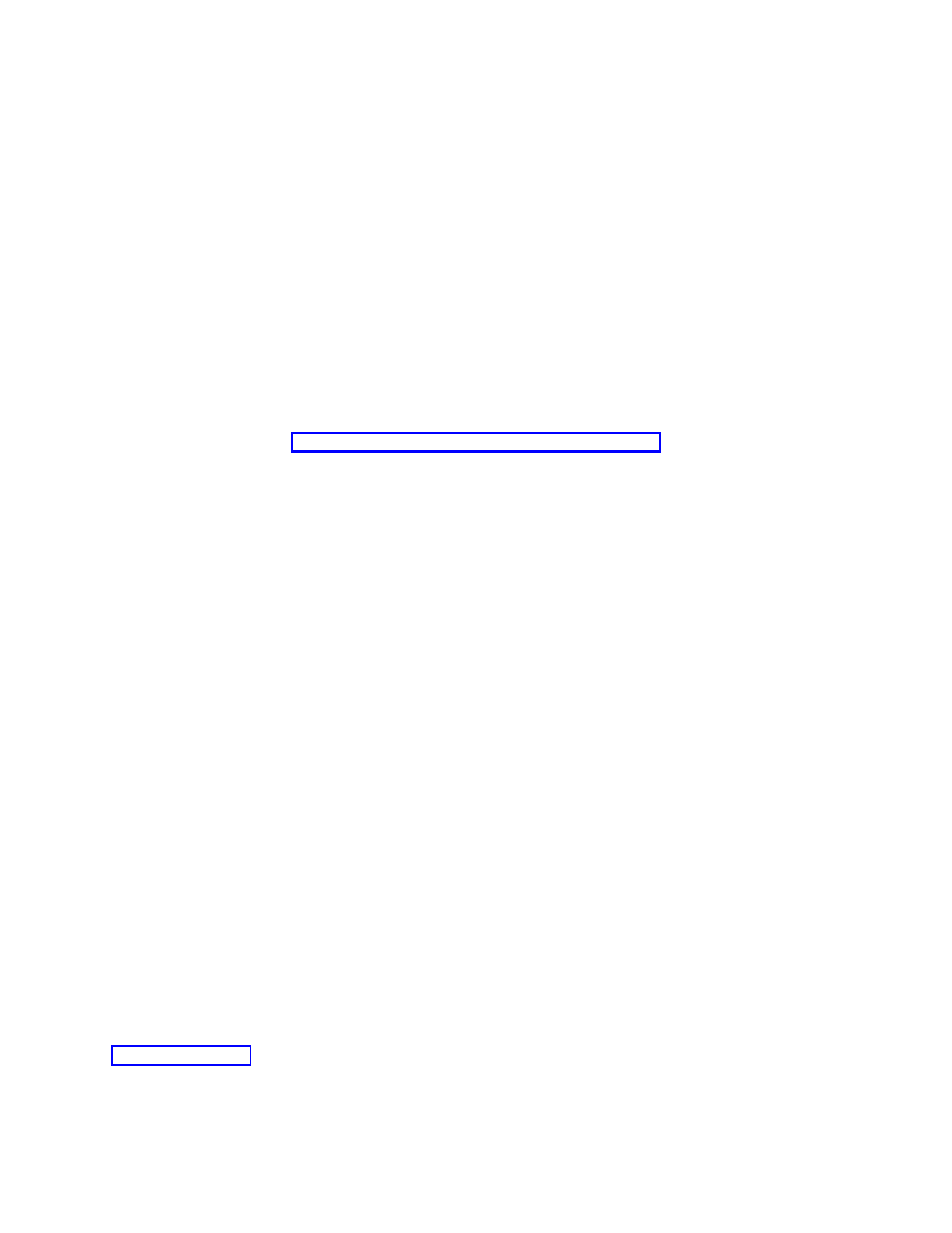
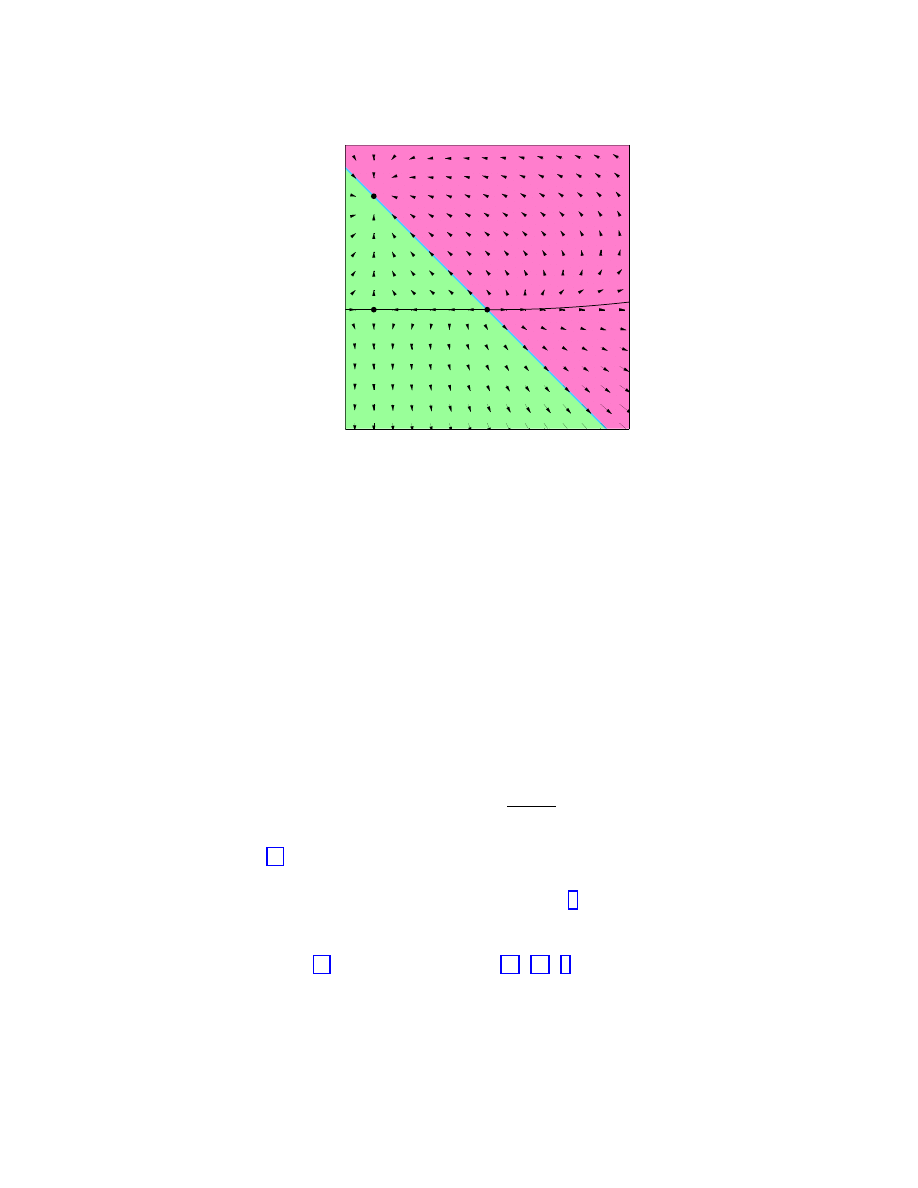
The dynamics of universes with Ω = Ω
M
+ Ω
Λ
are summarized in Figure (1), in which the
arrows indicate the evolution of these parameters in an expanding universe. (In a contracting
universe they would be reversed.) This is not a true phase-space plot, despite the superficial
similarities. One important difference is that a universe passing through one point can pass
through the same point again but moving backwards along its trajectory, by first going to
infinity and then turning around (recollapse).
Figure (1) includes three fixed points, at (Ω
M
, Ω
Λ
) equal to (0, 0), (0, 1), and (1, 0). The
attractor among these at (1, 0) is known as de Sitter space — a universe with no matter
density, dominated by a cosmological constant, and with scale factor growing exponentially
with time. The fact that this point is an attractor on the diagram is another way of under-
standing the cosmological constant problem. A universe with initial conditions located at a
generic point on the diagram will, after several expansion times, flow to de Sitter space if it
began above the recollapse line, and flow to infinity and back to recollapse if it began below
that line. Since our universe has undergone a large number of e-folds of expansion since
early times, it must have begun at a non-generic point in order not to have evolved either
to de Sitter space or to a Big Crunch. The only other two fixed points on the diagram are
the saddle point at (Ω
M
, Ω
Λ
) = (0, 0), corresponding to an empty universe, and the repulsive
fixed point at (Ω
M
, Ω
Λ
) = (1, 0), known as the Einstein-de Sitter solution. Since our uni-
verse is not empty, the favored solution from this combination of theoretical and empirical
arguments is the Einstein-de Sitter universe. The inflationary scenario [21, 22, 23] provides a
mechanism whereby the universe can be driven to the line Ω
M
+ Ω
Λ
= 1 (spatial flatness), so
11
0
0.5
1
1.5
2
Ω
M
−
1
−
0.5
0
0.5
1
Ω
Λ
Figure 1: Dynamics for Ω = Ω
M
+ Ω
Λ
. The arrows indicate the direction of evolution of the
parameters in an expanding universe.
Einstein-de Sitter is a natural expectation if we imagine that some unknown mechanism sets
Λ = 0. As discussed below, the observationally favored universe is located on this line but
away from the fixed points, near (Ω
M
, Ω
Λ
) = (0.3, 0.7). It is fair to conclude that naturalness
arguments have a somewhat spotty track record at predicting cosmological parameters.
2.3
Surveying the universe
The lookback time from the present day to an object at redshift z
∗
is given by
t
0
− t
∗
=
Z
t
0
t
∗
dt
=
Z
1
1/(1+z
∗
)
da
aH(a)
,
(36)
with H(a) given by (30). The age of the universe is obtained by taking the z
∗
→ ∞ (t
∗
→ 0)
limit. For Ω = Ω
M
= 1, this yields the familiar answer t
0
= (2/3)H
−1
0
; the age decreases as
Ω
M
is increased, and increases as Ω
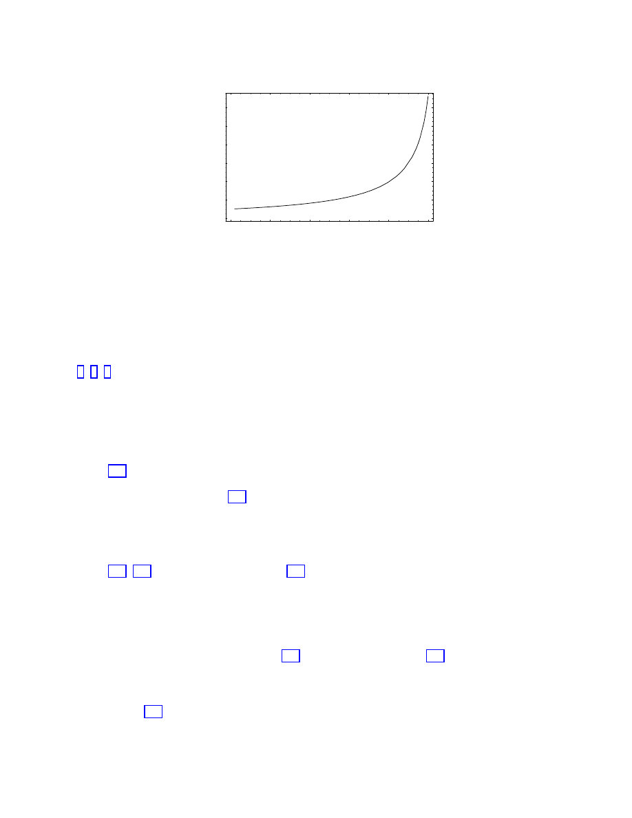
Λ
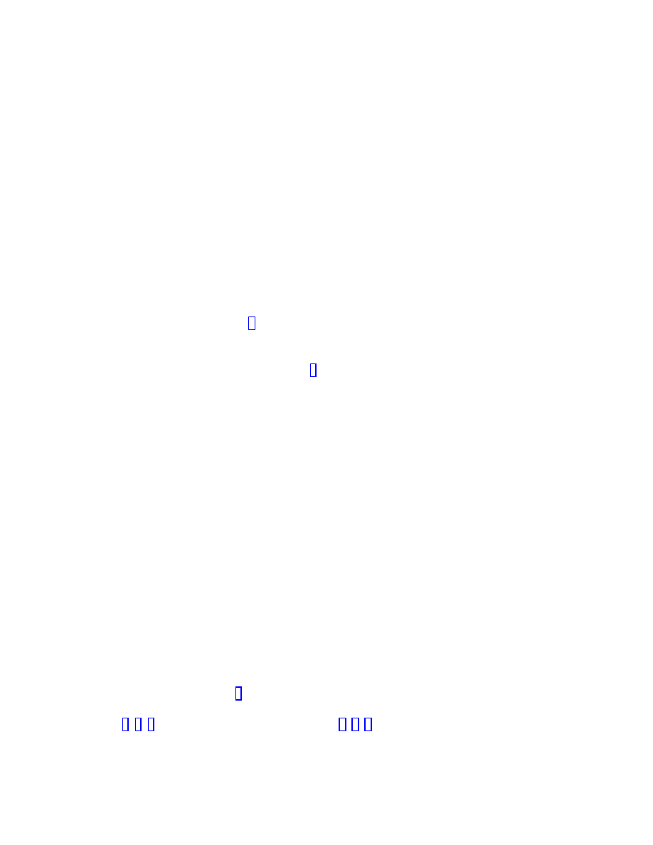
is increased. Figure (2) shows the expansion history
of the universe for different values of these parameters and H
0
fixed; it is clear how the
acceleration caused by Ω
Λ
leads to an older universe. There are analytic approximation
formulas which estimate (36) in various regimes [10, 11, 3], but generally the integral is
straightforward to perform numerically.
In a generic curved spacetime, there is no preferred notion of the distance between two
objects. Robertson-Walker spacetimes have preferred foliations, so it is possible to define
12
- 0.5
0
0.5
1
1.5
H
0
(t - t
0
)
0.25
0.5
0.75
1
1.25
1.5
1.75
2
a(t)
Figure 2: Expansion histories for different values of Ω
M
and Ω
Λ
. From top to bottom, the
curves describe (Ω
M
, Ω
Λ
) = (0.3, 0.7), (0.3, 0.0), (1.0, 0.0), and (4.0, 0.0).
sensible notions of the distance between comoving objects — those whose worldlines are
normal to the preferred slices. Placing ourselves at r = 0 in the coordinates defined by
(2), the coordinate distance r to another comoving object is independent of time. It can
be converted to a physical distance at any specified time t
∗
by multiplying by the scale
factor R
0
a(t
∗
), yielding a number which will of course change as the universe expands.
However, intervals along spacelike slices are not accessible to observation, so it is typically
more convenient to use distance measures which can be extracted from observable quantities.
These include the luminosity distance,
d
L
≡
s
L
4πF
,
(37)
where L is the intrinsic luminosity and F the measured flux; the proper-motion distance,
d
M
≡
u
˙θ
,
(38)
where u is the transverse proper velocity and ˙θ the observed angular velocity; and the
angular-diameter distance,
d
A
≡
D
θ
,
(39)
where D is the proper size of the object and θ its apparent angular size. All of these
definitions reduce to the usual notion of distance in a Euclidean space. In a Robertson-
Walker universe, the proper-motion distance turns out to equal the physical distance along
a spacelike slice at t = t
0
:
d
M
= R
0
r .
(40)
The three measures are related by
d
L
= (1 + z)d
M
= (1 + z)
2
d
A
,
(41)
13
so any one can be converted to any other for sources of known redshift.
The proper-motion distance between sources at redshift z
1
and z
2
can be computed by
using ds
2
= 0 along a light ray, where ds
2
is given by (2). We have
d
M
(z
1
, z
2
) = R
0
(r
2
− r
1
)
= R
0
sinn
"Z
t
2
t
1
dt
R
0
a(t)
#
=
1
H
0
q
|Ω
k0
|
sinn
"
H
0
q
|Ω
k0
|
Z
1/(1+z
2
)
1/(1+z
1
)
da
a
2
H(a)
#
,
(42)
where we have used (5) to solve for R
0
= 1/(H
0
q
|Ω
k0
|), H(a) is again given by (30), and
“sinn(x)” denotes sinh(x) when Ω
k0
< 0, sin(x) when Ω
k0
> 0, and x when Ω
k0
= 0. An
analytic approximation formula can be found in [24]. Note that, for large redshifts, the
dependence of the various distance measures on z is not necessarily monotonic.
The comoving volume element in a Robertson-Walker universe is given by
dV =
R
3
0
r
2
√
1
− kr
2
drdΩ ,
(43)
which can be integrated analytically to obtain the volume out to a distance d
M
:
V (d
M
) =
1
2H
3
0
Ω
k0
H
0
d
M
q
1 + H
2
0
Ω
k0
d
2
M
−
1
q
|Ω
k0
|
sinn
−1
(H
0
q
|Ω
k0
|d
M
)
,
(44)
where “sinn” is defined as below (42).
2.4
Structure formation
The introduction of a cosmological constant changes the relationship between the matter
density and expansion rate from what it would be in a matter-dominated universe, which in
turn influences the growth of large-scale structure. The effect is similar to that of a nonzero
spatial curvature, and complicated by hydrodynamic and nonlinear effects on small scales,
but is potentially detectable through sufficiently careful observations.
The analysis of the evolution of structure is greatly abetted by the fact that perturbations
start out very small (temperature anisotropies in the microwave background imply that
the density perturbations were of order 10
−5
at recombination), and linearized theory is
effective. In this regime, the fate of the fluctuations is in the hands of two competing effects:
the tendency of self-gravity to make overdense regions collapse, and the tendency of test
particles in the background expansion to move apart. Essentially, the effect of vacuum
energy is to contribute to expansion but not to the self-gravity of overdensities, thereby
acting to suppress the growth of perturbations [11, 13].
14
For sub-Hubble-radius perturbations in a cold dark matter component, a Newtonian
analysis suffices. (We may of course be interested in super-Hubble-radius modes, or the
evolution of interacting or relativistic particles, but the simple Newtonian case serves to
illustrate the relevant physical effect.) If the energy density in dynamical matter is dominated
by CDM, the linearized Newtonian evolution equation is
¨
δ
M
+ 2
˙a
a
˙δ
M
= 4πGρ
M
δ
M
.
(45)
The second term represents an effective frictional force due to the expansion of the universe,
characterized by a timescale ( ˙a/a)
−1
= H
−1
, while the right hand side is a forcing term with
characteristic timescale (4πGρ
M
)
−1/2
≈ Ω
−1/2
M
H
−1
. Thus, when Ω
M
≈ 1, these effects are
in balance and CDM perturbations gradually grow; when Ω
M
dips appreciably below unity
(as when curvature or vacuum energy begin to dominate), the friction term becomes more
important and perturbation growth effectively ends. In fact (45) can be directly solved [25]
to yield
δ
M
(a) =
5
2
H
2
0
Ω
M0
˙a
a
Z
a
0
H
−3
(a
0
) da
0
,
(46)
where H(a) is given by (30). There exist analytic approximations to this formula [3], as well
as analytic expressions for flat universes [26]. Note that this analysis is consistent only in the
linear regime; once perturbations on a given scale become of order unity, they break away
from the Hubble flow and begin to evolve as isolated systems.
3
Observational tests
It has been suspected for some time now that there are good reasons to think that a cosmology
with an appreciable cosmological constant is the best fit to what we know about the universe
[27, 28, 29, 30, 31, 32, 33, 34, 35]. However, it is only very recently that the observational
case has tightened up considerably, to the extent that, as the year 2000 dawns, more experts
than not believe that there really is a positive vacuum energy exerting a measurable effect
on the evolution of the universe. In this section I review the major approaches which have
led to this shift.
3.1
Type Ia supernovae
The most direct and theory-independent way to measure the cosmological constant would
be to actually determine the value of the scale factor as a function of time. Unfortunately,
the appearance of Ω
k
in formulae such as (42) renders this difficult. Nevertheless, with
sufficiently precise information about the dependence of a distance measure on redshift we
can disentangle the effects of spatial curvature, matter, and vacuum energy, and methods
along these lines have been popular ways to try to constrain the cosmological constant.
Astronomers measure distance in terms of the “distance modulus” m
− M, where m is
the apparent magnitude of the source and M its absolute magnitude. The distance modulus
15
is related to the luminosity distance via
m
− M = 5 log
10
[d
L
(Mpc)] + 25 .
(47)
Of course, it is easy to measure the apparent magnitude, but notoriously difficult to in-
fer the absolute magnitude of a distant object. Methods to estimate the relative absolute
luminosities of various kinds of objects (such as galaxies with certain characteristics) have
been pursued, but most have been plagued by unknown evolutionary effects or simply large
random errors [6].
Recently, significant progress has been made by using Type Ia supernovae as “standard-
izable candles”. Supernovae are rare — perhaps a few per century in a Milky-Way-sized
galaxy — but modern telescopes allow observers to probe very deeply into small regions of
the sky, covering a very large number of galaxies in a single observing run. Supernovae are
also bright, and Type Ia’s in particular all seem to be of nearly uniform intrinsic luminosity
(absolute magnitude M
∼ −19.5, typically comparable to the brightness of the entire host
galaxy in which they appear) [36]. They can therefore be detected at high redshifts (z
∼ 1),
allowing in principle a good handle on cosmological effects [37, 38].
The fact that all SNe Ia are of similar intrinsic luminosities fits well with our under-
standing of these events as explosions which occur when a white dwarf, onto which mass is
gradually accreting from a companion star, crosses the Chandrasekhar limit and explodes.
(It should be noted that our understanding of supernova explosions is in a state of develop-
ment, and theoretical models are not yet able to accurately reproduce all of the important
features of the observed events. See [39, 40, 41] for some recent work.) The Chandrasekhar
limit is a nearly-universal quantity, so it is not a surprise that the resulting explosions are of
nearly-constant luminosity. However, there is still a scatter of approximately 40% in the peak
brightness observed in nearby supernovae, which can presumably be traced to differences in
the composition of the white dwarf atmospheres. Even if we could collect enough data that
statistical errors could be reduced to a minimum, the existence of such an uncertainty would
cast doubt on any attempts to study cosmology using SNe Ia as standard candles.
Fortunately, the observed differences in peak luminosities of SNe Ia are very closely
correlated with observed differences in the shapes of their light curves: dimmer SNe decline
more rapidly after maximum brightness, while brighter SNe decline more slowly [42, 43, 44].
There is thus a one-parameter family of events, and measuring the behavior of the light curve
along with the apparent luminosity allows us to largely correct for the intrinsic differences
in brightness, reducing the scatter from 40% to less than 15% — sufficient precision to
distinguish between cosmological models. (It seems likely that the single parameter can
be traced to the amount of
56
Ni produced in the supernova explosion; more nickel implies
both a higher peak luminosity and a higher temperature and thus opacity, leading to a slower
decline. It would be an exaggeration, however, to claim that this behavior is well-understood
theoretically.)
Following pioneering work reported in [45], two independent groups have undertaken
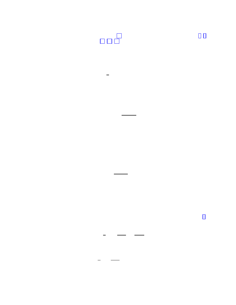
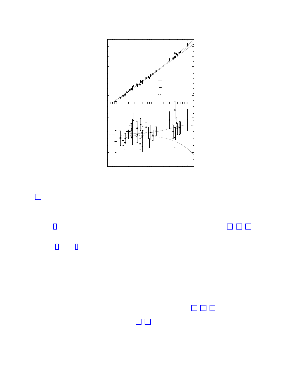
searches for distant supernovae in order to measure cosmological parameters. Figure (3)
shows the results for m
− M vs. z for the High-Z Supernova Team [46, 47, 48, 49], and
16
34
36
38
40
42
44
Ω
M
=0.24,
Ω
Λ
=0.76
Ω
M
=0.20,
Ω
Λ
=0.00
Ω
M
=1.00,
Ω
Λ
=0.00
m-M (mag)
MLCS
0.01
0.10
1.00
z
-0.5
0.0
0.5
∆
(m-M) (mag)
Figure 3: Hubble diagram (distance modulus vs. redshift) from the High-Z Supernova Team
[48]. The lines represent predictions from the cosmological models with the specified param-
eters. The lower plot indicates the difference between observed distance modulus and that
predicted in an open-universe model.
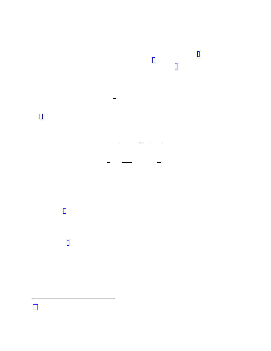
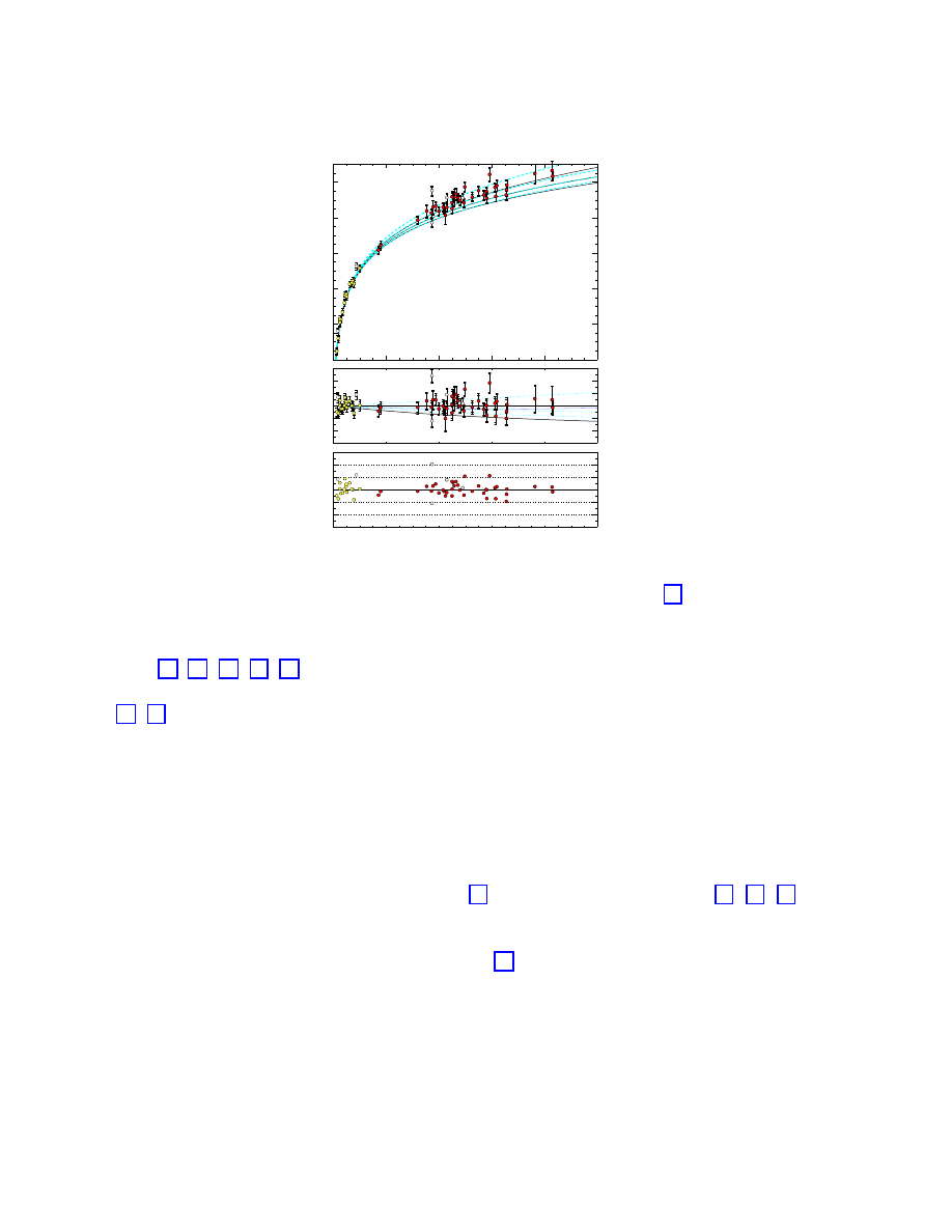
Figure (4) shows the equivalent results for the Supernova Cosmology Project [50, 51, 52].
Under the assumption that the energy density of the universe is dominated by matter and
vacuum components, these data can be converted into limits on Ω
M
and Ω
Λ
, as shown in
It is clear that the confidence intervals in the Ω
M
-Ω
Λ
plane are consistent for the two
groups, with somewhat tighter constraints obtained by the Supernova Cosmology Project,
who have more data points. The surprising result is that both teams favor a positive cos-
mological constant, and strongly rule out the traditional (Ω
M
, Ω
Λ
) = (1, 0) favorite universe.
They are even inconsistent with an open universe with zero cosmological constant, given
what we know about the matter density of the universe (see below).
Given the significance of these results, it is natural to ask what level of confidence we
should have in them. There are a number of potential sources of systematic error which
have been considered by the two teams; see the original papers [47, 48, 52] for a thorough
discussion. The two most worrisome possibilities are intrinsic differences between Type
Ia supernovae at high and low redshifts [53, 54], and possible extinction via intergalactic
17
Calan/Tololo
(Hamuy et al,
A.J. 1996)
Supernova
Cosmology
Project
effective
m
B
mag residual
standard deviation
(a)
(b)
(c)
(0.5,0.5)
(0, 0)
( 1, 0 )
(1, 0)
(1.5,–0.5)
(2, 0)
(Ω
Μ,
Ω
Λ
) =
( 0, 1 )
Flat
(0.28, 0.72)
(0.75, 0.25 )
(1, 0)
(0.5, 0.5 )
(0, 0)
(0, 1 )
(Ω
Μ ,
Ω
Λ
) =
Λ = 0
redshift
z
14
16
18
20
22
24
-1.5
-1.0
-0.5
0.0
0.5
1.0
1.5
0.0
0.2
0.4
0.6
0.8
1.0
-6
-4
-2
0
2
4
6
Figure 4: Hubble diagram from the Supernova Cosmology Project [52]. The bottom plot
shows the number of standard deviations of each point from the best-fit curve.
dust [55, 56, 57, 58, 59]. (There is also the fact that intervening weak lensing can change
the distance-magnitude relation, but this seems to be a small effect in realistic universes
[60, 61].) Both effects have been carefully considered, and are thought to be unimportant,
although a better understanding will be necessary to draw firm conclusions. Here, I will
briefly mention some of the relevant issues.
As thermonuclear explosions of white dwarfs, Type Ia supernovae can occur in a wide
variety of environments. Consequently, a simple argument against evolution is that the
high-redshift environments, while chronologically younger, should be a subset of all possible
low-redshift environments, which include regions that are “young” in terms of chemical and
stellar evolution. Nevertheless, even a small amount of evolution could ruin our ability to
reliably constrain cosmological parameters [53]. In their original papers [47, 48, 52], the
supernova teams found impressive consistency in the spectral and photometric properties of
Type Ia supernovae over a variety of redshifts and environments (e.g., in elliptical vs. spiral
galaxies). More recently, however, Riess et al. [54] have presented tentative evidence for a
systematic difference in the properties of high- and low-redshift supernovae, claiming that
the risetimes (from initial explosion to maximum brightness) were higher in the high-redshift
events. Apart from the issue of whether the existing data support this finding, it is not
immediately clear whether such a difference is relevant to the distance determinations: first,
because the risetime is not used in determining the absolute luminosity at peak brightness,
18
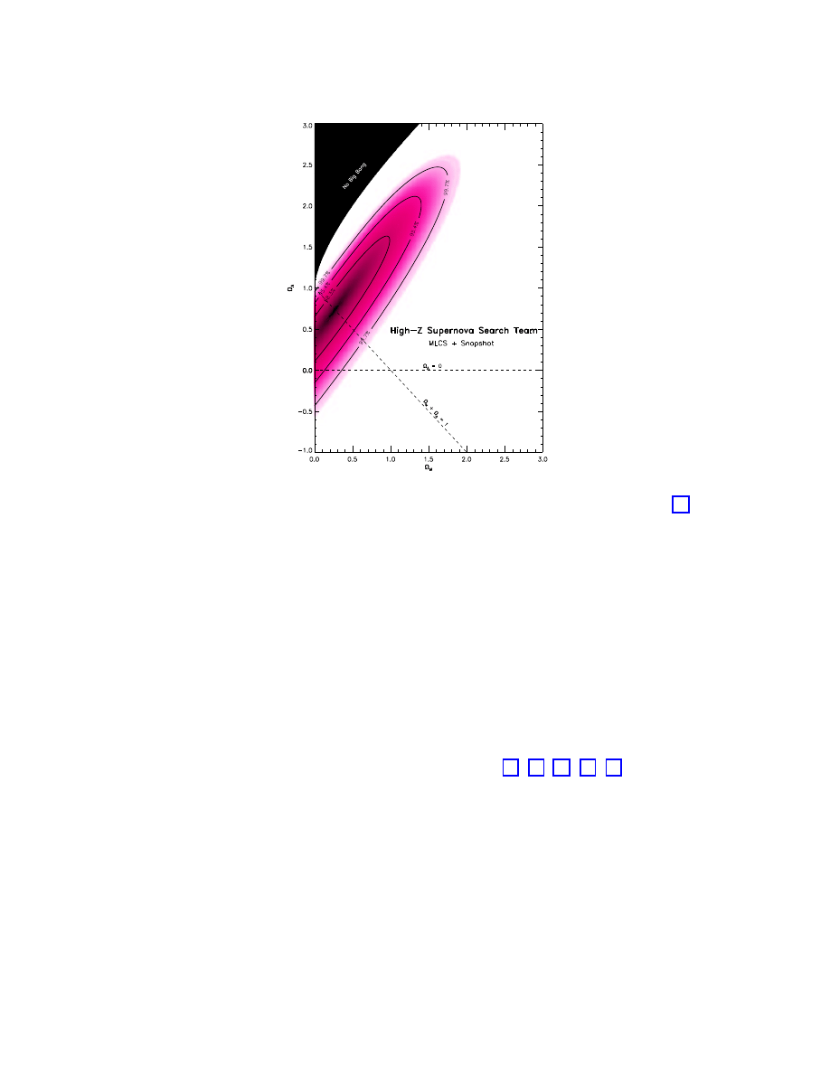
Figure 5: Constraints in the Ω
M
-Ω
Λ
plane from the High-Z Supernova Team [48].
and second, because a process which only affects the very early stages of the light curve is
most plausibly traced to differences in the outer layers of the progenitor, which may have a
negligible affect on the total energy output. Nevertheless, any indication of evolution could
bring into question the fundamental assumptions behind the entire program. It is therefore
essential to improve the quality of both the data and the theories so that these issues may
be decisively settled.
Other than evolution, obscuration by dust is the leading concern about the reliability
of the supernova results. Ordinary astrophysical dust does not obscure equally at all wave-
lengths, but scatters blue light preferentially, leading to the well-known phenomenon of
“reddening”. Spectral measurements by the two supernova teams reveal a negligible amount
of reddening, implying that any hypothetical dust must be a novel “grey” variety. This
possibility has been investigated by a number of authors [55, 56, 57, 58, 59]. These studies
have found that even grey dust is highly constrained by observations: first, it is likely to be
intergalactic rather than within galaxies, or it would lead to additional dispersion in the mag-
nitudes of the supernovae; and second, intergalactic dust would absorb ultraviolet/optical
radiation and re-emit it at far infrared wavelengths, leading to stringent constraints from
observations of the cosmological far-infrared background. Thus, while the possibility of ob-
scuration has not been entirely eliminated, it requires a novel kind of dust which is already
highly constrained (and may be convincingly ruled out by further observations).
According to the best of our current understanding, then, the supernova results indicat-
19
Ω
Μ
No Big Bang
1
2
0
1
2
3
expands foreve
r
Ω
Λ
Flat
Λ
= 0
Universe
-1
0
1
2
3
2
3
closed
open
90%
68%
99%
95%
recollapses eventu
ally
flat
Figure 6: Constraints in the Ω
M
-Ω
Λ
plane from the Supernova Cosmology Project [52].
ing an accelerating universe seem likely to be trustworthy. Needless to say, however, the
possibility of a heretofore neglected systematic effect looms menacingly over these studies.
Future experiments, including a proposed satellite dedicated to supernova cosmology [62],
will both help us improve our understanding of the physics of supernovae and allow a deter-
mination of the distance/redshift relation to sufficient precision to distinguish between the
effects of a cosmological constant and those of more mundane astrophysical phenomena. In
the meantime, it is important to obtain independent corroboration using other methods.
3.2
Cosmic microwave background
The discovery by the COBE satellite of temperature anisotropies in the cosmic microwave
background [63] inaugurated a new era in the determination of cosmological parameters. To
characterize the temperature fluctuations on the sky, we may decompose them into spherical
harmonics,
∆T
T
=
X
lm
a
lm
Y
lm
(θ, φ) ,
(48)
and express the amount of anisotropy at multipole moment l via the power spectrum,
C
l
=
h|a
lm
|
2
i .
(49)
20
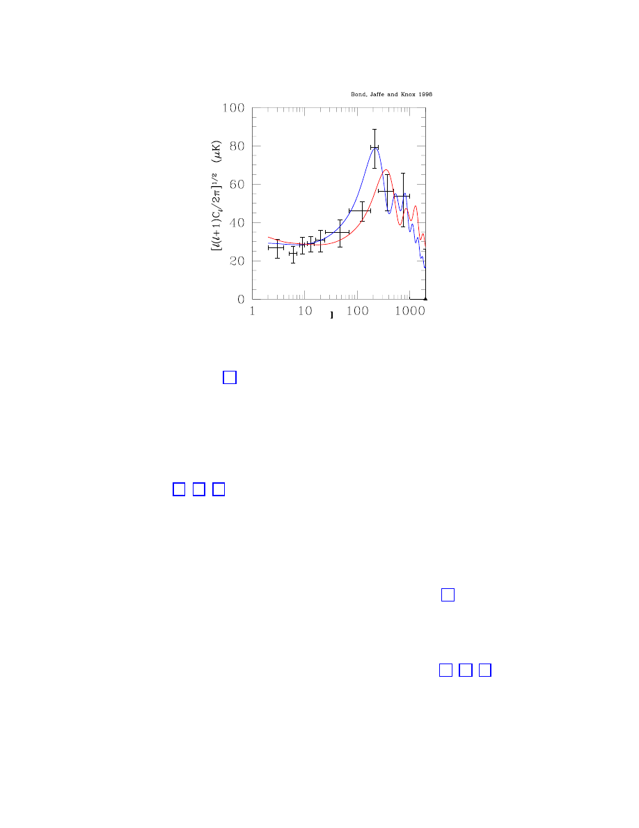
Figure 7: CMB data (binned) and two theoretical curves: the model with a peak at l
∼ 200
is a flat matter-dominated universe, while the one with a peak at l
∼ 400 is an open matter-
dominated universe. From [72].
Higher multipoles correspond to smaller angular separations on the sky, θ = 180
◦
/l. Within
any given family of models, C
l
vs. l will depend on the parameters specifying the particular
cosmology. Although the case is far from closed, evidence has been mounting in favor of a
specific class of models — those based on Gaussian, adiabatic, nearly scale-free perturbations
in a universe composed of baryons, radiation, and cold dark matter. (The inflationary
universe scenario [21, 22, 23] typically predicts these kinds of perturbations.)
Although the dependence of the C
l
’s on the parameters can be intricate, nature has
chosen not to test the patience of cosmologists, as one of the easiest features to measure —
the location in l of the first “Doppler peak”, an increase in power due to acoustic oscillations
— provides one of the most direct handles on the cosmic energy density, one of the most
interesting parameters. The first peak (the one at lowest l) corresponds to the angular
scale subtended by the Hubble radius H
−1
CMB
at the time when the CMB was formed (known
variously as “decoupling” or “recombination” or “last scattering”) [64]. The angular scale
at which we observe this peak is tied to the geometry of the universe: in a negatively
(positively) curved universe, photon paths diverge (converge), leading to a larger (smaller)
apparent angular size as compared to a flat universe. Since the scale H
−1
CMB
is set mostly by
microphysics, this geometrical effect is dominant, and we can relate the spatial curvature as
characterized by Ω to the observed peak in the CMB spectrum via [65, 66, 67]
l
peak
∼ 220Ω
−1/2
.
(50)
More details about the spectrum (height of the peak, features of the secondary peaks) will
21
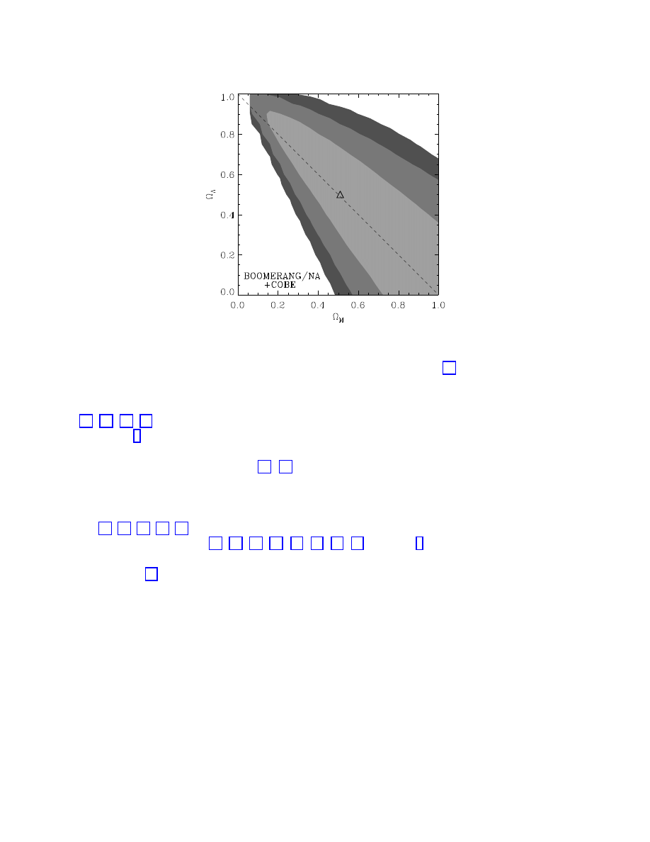
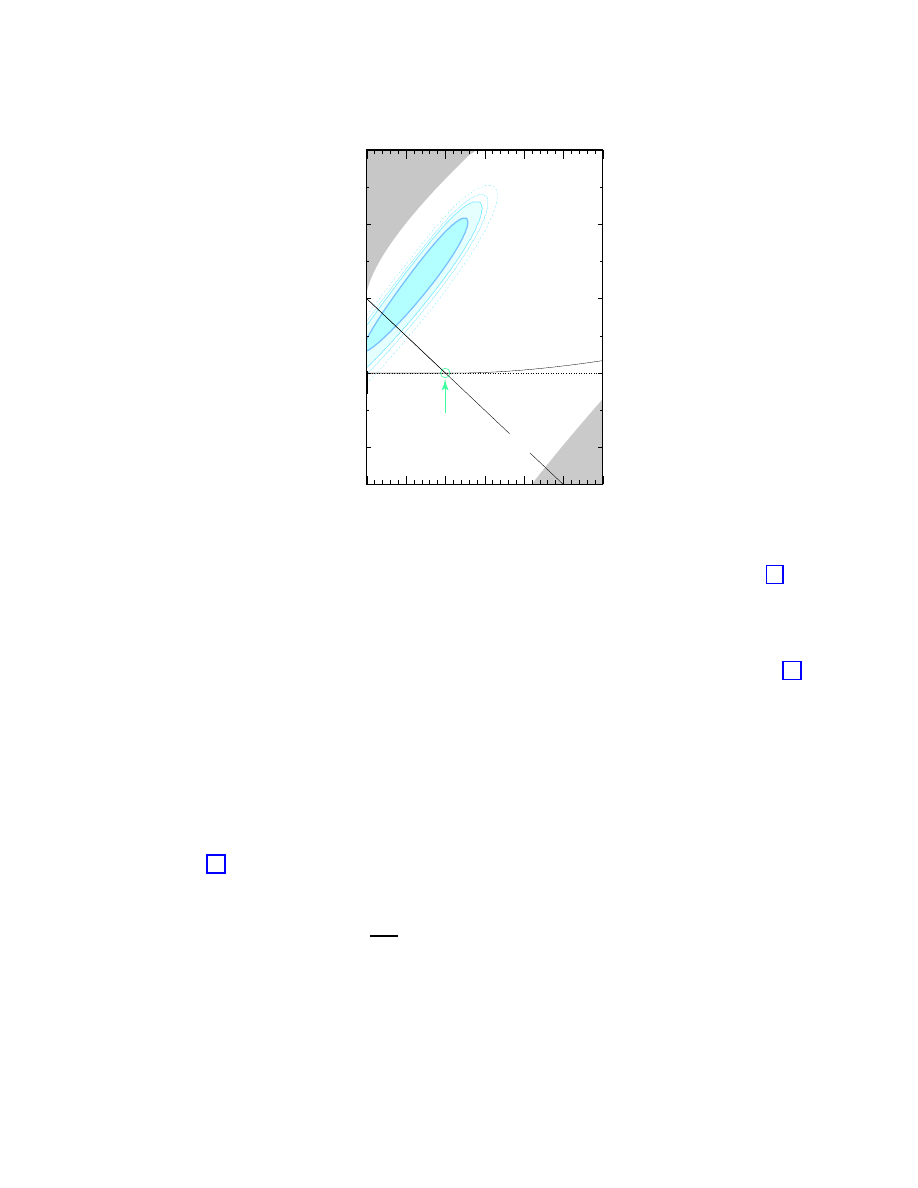
Figure 8:
Constraints in the Ω
M
-Ω
Λ
plane from the North American flight of the
BOOMERANG microwave background balloon experiment. From [74].
depend on other cosmological quantities, such as the Hubble constant and the baryon density
[68, 69, 70, 71].
Figure 7 shows a summary of data as of 1998, with various experimental results consoli-
dated into bins, along with two theoretical models. Since that time, the data have continued
to accumulate (see for example [73, 74]), and the near future should see a wealth of new
results of ever-increasing precision. It is clear from the figure that there is good evidence for
a peak at approximately l
peak
∼ 200, as predicted in a spatially-flat universe. This result can
be made more quantitative by fitting the CMB data to models with different values of Ω
M
and
Ω
Λ
[72, 75, 76, 77, 78], or by combining the CMB data with other sources, such as supernovae
or large-scale structure [79, 80, 49, 81, 82, 83, 84, 85]. Figure 8 shows the constraints from
the CMB in the Ω
M
-Ω
Λ
plane, using data from the 1997 test flight of the BOOMERANG
experiment [74]. (Although the data used to make this plot are essentially independent of
those shown in the previous figure, the constraints obtained are nearly the same.) It is clear
that the CMB data provide constraints which are complementary to those obtained using
supernovae; the two approaches yield confidence contours which are nearly orthogonal in the
Ω
M
-Ω
Λ
plane. The region of overlap is in the vicinity of (Ω
M
, Ω
Λ
) = (0.3, 0.7), which we will
see below is also consistent with other determinations.
3.3
Matter density
Many cosmological tests, such as the two just discussed, will constrain some combination of
Ω
M
and Ω
Λ
. It is therefore useful to consider tests of Ω
M
alone, even if our primary goal is to
22
determine Ω
Λ
. (In truth, it is also hard to constrain Ω
M
alone, as almost all methods actually
constrain some combination of Ω
M
and the Hubble constant h = H
0
/(100 km/sec/Mpc); the
HST Key Project on the extragalactic distance scale finds h = 0.71
± 0.06 [86], which is
consistent with other methods [87], and what I will assume below.)
For years, determinations of Ω
M
based on dynamics of galaxies and clusters have yielded
values between approximately 0.1 and 0.4 — noticeably larger than the density parameter in
baryons as inferred from primordial nucleosynthesis, Ω
B
= (0.019
±0.001)h
−2
but noticeably smaller than the critical density. The last several years have witnessed a
number of new methods being brought to bear on the question; the quantitative results have
remained unchanged, but our confidence in them has increased greatly.
A thorough discussion of determinations of Ω
M
requires a review all its own, and good
ones are available [90, 91, 92, 87, 93]. Here I will just sketch some of the important methods.
The traditional method to estimate the mass density of the universe is to “weigh” a cluster
of galaxies, divide by its luminosity, and extrapolate the result to the universe as a whole.
Although clusters are not representative samples of the universe, they are sufficiently large
that such a procedure has a chance of working. Studies applying the virial theorem to cluster
dynamics have typically obtained values Ω
M
= 0.2
± 0.1 [94, 90, 91]. Although it is possible
that the global value of M/L differs appreciably from its value in clusters, extrapolations
from small scales do not seem to reach the critical density [95]. New techniques to weigh the
clusters, including gravitational lensing of background galaxies [96] and temperature profiles
of the X-ray gas [97], while not yet in perfect agreement with each other, reach essentially
similar conclusions.
Rather than measuring the mass relative to the luminosity density, which may be different
inside and outside clusters, we can also measure it with respect to the baryon density [98],
which is very likely to have the same value in clusters as elsewhere in the universe, simply
because there is no way to segregate the baryons from the dark matter on such large scales.
Most of the baryonic mass is in the hot intracluster gas [99], and the fraction f
gas
of total
mass in this form can be measured either by direct observation of X-rays from the gas [100]
or by distortions of the microwave background by scattering off hot electrons (the Sunyaev-
Zeldovich effect) [101], typically yielding 0.1
≤ f
gas
≤ 0.2. Since primordial nucleosynthesis
provides a determination of Ω
B
∼ 0.04, these measurements imply
Ω
M
= Ω
B
/f
gas
= 0.3
± 0.1 ,
(51)
consistent with the value determined from mass to light ratios.
Another handle on the density parameter in matter comes from properties of clusters
at high redshift. The very existence of massive clusters has been used to argue in favor of
Ω
M
∼ 0.2 [102], and the lack of appreciable evolution of clusters from high redshifts to the
present [103, 104] provides additional evidence that Ω
M
< 1.0.
The story of large-scale motions is more ambiguous. The peculiar velocities of galaxies are
sensitive to the underlying mass density, and thus to Ω
M
, but also to the “bias” describing
the relative amplitude of fluctuations in galaxies and mass [90, 105]. Difficulties both in
measuring the flows and in disentangling the mass density from other effects make it difficult
23
to draw conclusions at this point, and at present it is hard to say much more than 0.2
≤
Ω
M
≤ 1.0.
Finally, the matter density parameter can be extracted from measurements of the power
spectrum of density fluctuations (see for example [106]). As with the CMB, predicting the
power spectrum requires both an assumption of the correct theory and a specification of a
number of cosmological parameters. In simple models (e.g., with only cold dark matter and
baryons, no massive neutrinos), the spectrum can be fit (once the amplitude is normalized) by
a single “shape parameter”, which is found to be equal to Γ = Ω
M
h. (For more complicated
models see [107].) Observations then yield Γ
∼ 0.25, or Ω
M
∼ 0.36. For a more careful
comparison between models and observations, see [108, 109, 110, 111].
Thus, we have a remarkable convergence on values for the density parameter in matter:
0.1
≤ Ω
M
≤ 0.4 .
(52)
Even without the supernova results, this determination in concert with the CMB measure-
ments favoring a flat universe provide a strong case for a nonzero cosmological constant.
3.4
Gravitational lensing
The volume of space back to a specified redshift, given by (44), depends sensitively on Ω
Λ
.
Consequently, counting the apparent density of observed objects, whose actual density per
cubic Mpc is assumed to be known, provides a potential test for the cosmological constant
[112, 113, 114, 3]. Like tests of distance vs. redshift, a significant problem for such methods
is the luminosity evolution of whatever objects one might attempt to count. A modern
attempt to circumvent this difficulty is to use the statistics of gravitational lensing of distant
galaxies; the hope is that the number of condensed objects which can act as lenses is less
sensitive to evolution than the number of visible objects.
In a spatially flat universe, the probability of a source at redshift z
s
being lensed, relative
to the fiducial (Ω
M
= 1, Ω
Λ
= 0) case, is given by
P
lens
=
15
4
h
1
− (1 + z
s
)
−1/2
i
−3
Z
a
s
1
H
0
H(a)
"
d
A
(0, a)d
A
(a, a
s
)
d
A
(0, a
s
)
#
da ,
(53)
where a
s
= 1/(1 + z
s
). As shown in Figure (9), the probability rises dramatically as Ω
Λ
is
increased to unity as we keep Ω fixed. Thus, the absence of a large number of such lenses
would imply an upper limit on Ω
Λ
.
Analysis of lensing statistics is complicated by uncertainties in evolution, extinction,
and biases in the lens discovery procedure. It has been argued [115, 116] that the existing
data allow us to place an upper limit of Ω
Λ
< 0.7 in a flat universe. However, other
groups [117, 118] have claimed that the current data actually favor a nonzero cosmological
constant. The near future will bring larger, more objective surveys, which should allow these
ambiguities to be resolved. Other manifestations of lensing can also be used to constrain
Ω
Λ
, including statistics of giant arcs [119], deep weak-lensing surveys [120], and lensing in
the Hubble Deep Field [121].
24
0
0.2
0.4
0.6
0.8
1
Ω
Λ
0
2
4
6
8
10
12
Lens
Probability
Figure 9: Gravitational lens probabilities in a flat universe with Ω
M
+ Ω
Λ
= 1, relative to
Ω
M
= 1, Ω
Λ
= 0, for a source at z = 2.
3.5
Other tests
There is a tremendous variety of ways in which a nonzero cosmological constant can manifest
itself in observable phenomena. Here is an incomplete list of additional possibilities; see also
[3, 7, 8].
• Observations of numbers of objects vs. redshift are a potentially sensitive test of cos-
mological parameters if evolutionary effects can be brought under control. Although it
is hard to account for the luminosity evolution of galaxies, it may be possible to indi-
rectly count dark halos by taking into account the rotation speeds of visible galaxies,
and upcoming redshift surveys could be used to constrain the volume/redshift relation
[122].
• Alcock and Paczynski [123] showed that the relationship between the apparent trans-
verse and radial sizes of an object of cosmological size depends on the expansion history
of the universe. Clusters of galaxies would be possible candidates for such a measure-
ment, but they are insufficiently isotropic; alternatives, however, have been proposed,
using for example the quasar correlation function as determined from redshift surveys
[124, 125], or the Lyman-α forest [126].
• In a related effect, the dynamics of large-scale structure can be affected by a nonzero
cosmological constant; if a protocluster, for example, is anisotropic, it can begin to
contract along a minor axis while the universe is matter-dominated and along its major
axis while the universe is vacuum-dominated. Although small, such effects may be
observable in individual clusters [127] or in redshift surveys [128].
• A different version of the distance-redshift test uses extended lobes of radio galaxies as
modified standard yardsticks. Current observations disfavor universes with Ω
M
near
unity ([129], and references therein).
25
• Inspiralling compact binaries at cosmological distances are potential sources of gravi-
tational waves. It turns out that the redshift distribution of events is sensitive to the
cosmological constant; although speculative, it has been proposed that advanced LIGO
detectors could use this effect to provide measurements of Ω
Λ
• Finally, consistency of the age of the universe and the ages of its oldest constituents
is a classic test of the expansion history. If stars were sufficiently old and H
0
and Ω
M
were sufficiently high, a positive Ω
Λ
would be necessary to reconcile the two, and this
situation has occasionally been thought to hold. Measurements of geometric parallax
to nearby stars from the Hipparcos satellite have, at the least, called into question
previous determinations of the ages of the oldest globular clusters, which are now
thought to be perhaps 12 billion rather than 15 billion years old (see the discussion in
[87]). It is therefore unclear whether the age issue forces a cosmological constant upon
us, but by now it seems forced upon us for other reasons.
4
Physics issues
In Section (1.3) we discussed the large difference between the magnitude of the vacuum
energy expected from zero-point fluctuations and scalar potentials, ρ
theor
Λ
∼ 2×10
110
erg/cm
3
,
and the value we apparently observe, ρ
(obs)
Λ
∼ 2 × 10
−10
erg/cm
3
(which may be thought of
as an upper limit, if we wish to be careful). It is somewhat unfair to characterize this
discrepancy as a factor of 10
120
, since energy density can be expressed as a mass scale to the
fourth power. Writing ρ
Λ
= M
4
vac
, we find M
(theory)
vac
∼ M
Pl
∼ 10
18
GeV and M
(obs)
vac
∼ 10
−3
eV,
so a more fair characterization of the problem would be
M
(theory)
vac
M
(obs)
vac
∼ 10
30
.
(54)
Of course, thirty orders of magnitude still constitutes a difference worthy of our attention.
Although the mechanism which suppresses the naive value of the vacuum energy is un-
known, it seems easier to imagine a hypothetical scenario which makes it exactly zero than
one which sets it to just the right value to be observable today. (Keeping in mind that it is
the zero-temperature, late-time vacuum energy which we want to be small; it is expected to
change at phase transitions, and a large value in the early universe is a necessary component
of inflationary universe scenarios [21, 22, 23].) If the recent observations pointing toward a
cosmological constant of astrophysically relevant magnitude are confirmed, we will be faced
with the challenge of explaining not only why the vacuum energy is smaller than expected,
but also why it has the specific nonzero value it does.
4.1
Supersymmetry
Although initially investigated for other reasons, supersymmetry (SUSY) turns out to have
a significant impact on the cosmological constant problem, and may even be said to solve it
26
halfway. SUSY is a spacetime symmetry relating fermions and bosons to each other. Just
as ordinary symmetries are associated with conserved charges, supersymmetry is associated
with “supercharges” Q
α
, where α is a spinor index (for introductions see [131, 132, 133]).
As with ordinary symmetries, a theory may be supersymmetric even though a given state is
not supersymmetric; a state which is annihilated by the supercharges, Q
α
|ψi = 0, preserves
supersymmetry, while states with Q
α
|ψi 6= 0 are said to spontaneously break SUSY.
Let’s begin by considering “globally supersymmetric” theories, which are defined in flat
spacetime (obviously an inadequate setting in which to discuss the cosmological constant, but
we have to start somewhere). Unlike most non-gravitational field theories, in supersymmetry
the total energy of a state has an absolute meaning; the Hamiltonian is related to the
supercharges in a straightforward way:
H =
X
α
{Q
α
, Q
†
α
} ,
(55)
where braces represent the anticommutator. Thus, in a completely supersymmetric state (in
which Q
α
|ψi = 0 for all α), the energy vanishes automatically, hψ|H|ψi = 0 [134]. More
concretely, in a given supersymmetric theory we can explicitly calculate the contributions
to the energy from vacuum fluctuations and from the scalar potential V . In the case of
vacuum fluctuations, contributions from bosons are exactly canceled by equal and opposite
contributions from fermions when supersymmetry is unbroken. Meanwhile, the scalar-field
potential in supersymmetric theories takes on a special form; scalar fields φ
i
must be complex
(to match the degrees of freedom of the fermions), and the potential is derived from a function
called the superpotential W (φ
i
) which is necessarily holomorphic (written in terms of φ
i
and
not its complex conjugate ¯
φ
i
). In the simple Wess-Zumino models of spin-0 and spin-1/2
fields, for example, the scalar potential is given by
V (φ
i
, ¯
φ
j
) =
X
i
|∂
i
W
|
2
,
(56)
where ∂
i
W = ∂W/∂φ
i
. In such a theory, one can show that SUSY will be unbroken only for
values of φ
i
such that ∂
i
W = 0, implying V (φ
i
, ¯
φ
j
) = 0.
So the vacuum energy of a supersymmetric state in a globally supersymmetric theory
will vanish. This represents rather less progress than it might appear at first sight, since: 1.)
Supersymmetric states manifest a degeneracy in the mass spectrum of bosons and fermions,
a feature not apparent in the observed world; and 2.) The above results imply that non-
supersymmetric states have a positive-definite vacuum energy. Indeed, in a state where
SUSY was broken at an energy scale M
SUSY
, we would expect a corresponding vacuum
energy ρ
Λ
∼ M
4
SUSY
. In the real world, the fact that accelerator experiments have not
discovered superpartners for the known particles of the Standard Model implies that M
SUSY
is of order 10
3
GeV or higher. Thus, we are left with a discrepancy
M
SUSY
M
vac
≥ 10
15
.
(57)
27
Comparison of this discrepancy with the naive discrepancy (54) is the source of the claim
that SUSY can solve the cosmological constant problem halfway (at least on a log scale).
As mentioned, however, this analysis is strictly valid only in flat space. In curved space-
time, the global transformations of ordinary supersymmetry are promoted to the position-
dependent (gauge) transformations of supergravity. In this context the Hamiltonian and
supersymmetry generators play different roles than in flat spacetime, but it is still possible
to express the vacuum energy in terms of a scalar field potential V (φ
i
, ¯
φ
j
). In supergravity V
depends not only on the superpotential W (φ
i
), but also on a “K¨ahler potential” K(φ
i
, ¯
φ
j
),
and the K¨ahler metric K
i¯
constructed from the K¨ahler potential by K
i¯
= ∂
2
K/∂φ
i
∂ ¯
φ
j
.
(The basic role of the K¨ahler metric is to define the kinetic term for the scalars, which takes
the form g
µν
K
i¯
∂
µ
φ
i
∂
ν
¯
φ
j
.) The scalar potential is
V (φ
i
, ¯
φ
j
) = e
K/M
2
Pl
h
K
i¯
(D
i
W )(D
¯
¯
W )
− 3M
−2
Pl
|W |
2
i
,
(58)
where D
i
W is the K¨ahler derivative,
D
i
W = ∂
i
W + M
−2
Pl
(∂
i
K)W .
(59)
Note that, if we take the canonical K¨ahler metric K
i¯
= δ
i¯
, in the limit M
Pl
→ ∞ (G → 0) the
first term in square brackets reduces to the flat-space result (56). But with gravity, in addition
to the non-negative first term we find a second term providing a non-positive contribution.
Supersymmetry is unbroken when D
i
W = 0; the effective cosmological constant is thus non-
positive. We are therefore free to imagine a scenario in which supersymmetry is broken in
exactly the right way, such that the two terms in parentheses cancel to fantastic accuracy,
but only at the cost of an unexplained fine-tuning (see for example [135]). At the same time,
supergravity is not by itself a renormalizable quantum theory, and therefore it may not be
reasonable to hope that a solution can be found purely within this context.
4.2
String theory
Unlike supergravity, string theory appears to be a consistent and well-defined theory of
quantum gravity, and therefore calculating the value of the cosmological constant should,
at least in principle, be possible. On the other hand, the number of vacuum states seems
to be quite large, and none of them (to the best of our current knowledge) features three
large spatial dimensions, broken supersymmetry, and a small cosmological constant. At the
same time, there are reasons to believe that any realistic vacuum of string theory must be
strongly coupled [136]; therefore, our inability to find an appropriate solution may simply
be due to the technical difficulty of the problem. (For general introductions to string theory,
see [137, 138]; for cosmological issues, see [139, 140]).
String theory is naturally formulated in more than four spacetime dimensions. Studies
of duality symmetries have revealed that what used to be thought of as five distinct ten-
dimensional superstring theories — Type I, Types IIA and IIB, and heterotic theories based
on gauge groups E(8)
×E(8) and SO(32) — are, along with eleven-dimensional supergravity,
28
different low-energy weak-coupling limits of a single underlying theory, sometimes known as
M-theory. In each of these six cases, the solution with the maximum number of uncompact-
ified, flat spacetime dimensions is a stable vacuum preserving all of the supersymmetry. To
bring the theory closer to the world we observe, the extra dimensions can be compactified
on a manifold whose Ricci tensor vanishes. There are a large number of possible compacti-
fications, many of which preserve some but not all of the original supersymmetry. If enough
SUSY is preserved, the vacuum energy will remain zero; generically there will be a manifold
of such states, known as the moduli space.
Of course, to describe our world we want to break all of the supersymmetry. Investiga-
tions in contexts where this can be done in a controlled way have found that the induced
cosmological constant vanishes at the classical level, but a substantial vacuum energy is typ-
ically induced by quantum corrections [137]. Moore [141] has suggested that Atkin-Lehner
symmetry, which relates strong and weak coupling on the string worldsheet, can enforce
the vanishing of the one-loop quantum contribution in certain models (see also [142, 143]);
generically, however, there would still be an appreciable contribution at two loops.
Thus, the search is still on for a four-dimensional string theory vacuum with broken
supersymmetry and vanishing (or very small) cosmological constant. (See [144] for a general
discussion of the vacuum problem in string theory.) The difficulty of achieving this in
conventional models has inspired a number of more speculative proposals, which I briefly list
here.
• In three spacetime dimensions supersymmetry can remain unbroken, maintaining a
zero cosmological constant, in such a way as to break the mass degeneracy between
bosons and fermions [145]. This mechanism relies crucially on special properties of
spacetime in (2+1) dimensions, but in string theory it sometimes happens that the
strong-coupling limit of one theory is another theory in one higher dimension [146, 147].
• More generally, it is now understood that (at least in some circumstances) string theory
obeys the “holographic principle”, the idea that a theory with gravity in D dimensions
is equivalent to a theory without gravity in D
−1 dimensions [148, 149]. In a holographic
theory, the number of degrees of freedom in a region grows as the area of its boundary,
rather than as its volume. Therefore, the conventional computation of the cosmological
constant due to vacuum fluctuations conceivably involves a vast overcounting of degrees
of freedom. We might imagine that a more correct counting would yield a much smaller
estimate of the vacuum energy [150, 151, 152, 153], although no reliable calculation
has been done as yet.
• The absence of manifest SUSY in our world leads us to ask whether the beneficial as-
pect of canceling contributions to the vacuum energy could be achieved even without
a truly supersymmetric theory. Kachru, Kumar and Silverstein [154] have constructed
such a string theory, and argue that the perturbative contributions to the cosmolog-
ical constant should vanish (although the actual calculations are somewhat delicate,
and not everyone agrees [155]). If such a model could be made to work, it is possi-
29
ble that small non-perturbative effects could generate a cosmological constant of an
astrophysically plausible magnitude [156].
• A novel approach to compactification starts by imagining that the fields of the Stan-
dard Model are confined to a (3+1)-dimensional manifold (or “brane”, in string theory
parlance) embedded in a larger space. While gravity is harder to confine to a brane,
phenomenologically acceptable scenarios can be constructed if either the extra dimen-
sions are any size less than a millimeter [157, 158, 159, 160, 161], or if there is significant
spacetime curvature in a non-compact extra dimension [162, 163, 164]. Although these
scenarios do not offer a simple solution to the cosmological constant problem, the
relationship between the vacuum energy and the expansion rate can differ from our
conventional expectation (see for example [165, 166]), and one is free to imagine that
further study may lead to a solution in this context (see for example [167, 168]).
Of course, string theory might not be the correct description of nature, or its current for-
mulation might not be directly relevant to the cosmological constant problem. For example,
a solution may be provided by loop quantum gravity [169], or by a composite graviton [170].
It is probably safe to believe that a significant advance in our understanding of fundamental
physics will be required before we can demonstrate the existence of a vacuum state with
the desired properties. (Not to mention the equally important question of why our world is
based on such a state, rather than one of the highly supersymmetric states that appear to
be perfectly good vacua of string theory.)
4.3
The anthropic principle
The anthropic principle [171, 172] is essentially the idea that some of the parameters charac-
terizing the universe we observe may not be determined directly by the fundamental laws of
physics, but also by the truism that intelligent observers will only ever experience conditions
which allow for the existence of intelligent observers. Many professional cosmologists view
this principle in much the same way as many traditional literary critics view deconstruction
— as somehow simultaneously empty of content and capable of working great evil. Anthropic
arguments are easy to misuse, and can be invoked as a way out of doing the hard work of
understanding the real reasons behind why we observe the universe we do. Furthermore, a
sense of disappointment would inevitably accompany the realization that there were limits
to our ability to unambiguously and directly explain the observed universe from first prin-
ciples. It is nevertheless possible that some features of our world have at best an anthropic
explanation, and the value of the cosmological constant is perhaps the most likely candidate.
In order for the tautology that “observers will only observe conditions which allow for
observers” to have any force, it is necessary for there to be alternative conditions — parts
of the universe, either in space, time, or branches of the wavefunction — where things are
different. In such a case, our local conditions arise as some combination of the relative
abundance of different environments and the likelihood that such environments would give
rise to intelligence. Clearly, the current state of the art doesn’t allow us to characterize
30
the full set of conditions in the entire universe with any confidence, but modern theories
of inflation and quantum cosmology do at least allow for the possibility of widely disparate
parts of the universe in which the “constants of nature” take on very different values (for
recent examples see [173, 174, 175, 176, 177, 178, 179]). We are therefore faced with the task
of estimating quantitatively the likelihood of observing any specific value of Λ within such a
scenario.
The most straightforward anthropic constraint on the vacuum energy is that it must not
be so high that galaxies never form [180]. From the discussion in Section (2.4), we know
that overdense regions do not collapse once the cosmological constant begins to dominate the
universe; if this happens before the epoch of galaxy formation, the universe will be devoid
of galaxies, and thus of stars and planets, and thus (presumably) of intelligent life. The
condition that Ω
Λ
(z
gal
)
≤ Ω
M
(z
gal
) implies
Ω
Λ0
Ω
M0
≤ a
−3
gal
= (1 + z
gal
)
3
∼ 125 ,
(60)
where we have taken the redshift of formation of the first galaxies to be z
gal
∼ 4. Thus, the
cosmological constant could be somewhat larger than observation allows and still be consis-
tent with the existence of galaxies. (This estimate, like the ones below, holds parameters
such as the amplitude of density fluctuations fixed while allowing Ω
Λ
to vary; depending on
one’s model of the universe of possibilities, it may be more defensible to vary a number of
parameters at once. See for example [181, 182, 172].)
However, it is better to ask what is most likely value of Ω
Λ
, i.e. what is the value that
would be experienced by the largest number of observers [183, 184]? Since a universe with
Ω
Λ0
/Ω
M0
∼ 1 will have many more galaxies than one with Ω
Λ0
/Ω
M0
∼ 100, it is quite
conceivable that most observers will measure something close to the former value. The
probability measure for observing a value of ρ
Λ
can be decomposed as
d
P(ρ
Λ
) = ν(ρ
Λ
)
P
∗
(ρ
Λ
)dρ
Λ
,
(61)
where
P
∗
(ρ
Λ
)dρ
Λ
is the a priori probability measure (whatever that might mean) for ρ
Λ
,
and ν(ρ
Λ
) is the average number of galaxies which form at the specified value of ρ
Λ
. Martel,
Shapiro and Weinberg [185] have presented a calculation of ν(ρ
Λ
) using a spherical-collapse
model. They argue that it is natural to take the a priori distribution to be a constant,
since the allowed range of ρ
Λ
is very far from what we would expect from particle-physics
scales. Garriga and Vilenkin [186] argue on the basis of quantum cosmology that there can
be a significant departure from a constant a priori distribution. However, in either case the
conclusion is that an observed Ω
Λ0
of the same order of magnitude as Ω
M0
is by no means
extremely unlikely (which is probably the best one can hope to say given the uncertainties
in the calculation).
Thus, if one is willing to make the leap of faith required to believe that the value of the
cosmological constant is chosen from an ensemble of possibilities, it is possible to find an
“explanation” for its current value (which, given its unnaturalness from a variety of perspec-
tives, seems otherwise hard to understand). Perhaps the most significant weakness of this
31
point of view is the assumption that there are a continuum of possibilities for the vacuum
energy density. Such possibilities correspond to choices of vacuum states with arbitrarily
similar energies. If these states were connected to each other, there would be local fluc-
tuations which would appear to us as massless fields, which are not observed (see Section
4.5). If on the other hand the vacua are disconnected, it is hard to understand why all
possible values of the vacuum energy are represented, rather than the differences in energies
between different vacua being given by some characteristic particle-physics scale such as M
Pl
or M
SUSY
. (For one scenario featuring discrete vacua with densely spaced energies, see [187].)
It will therefore (again) require advances in our understanding of fundamental physics before
an anthropic explanation for the current value of the cosmological constant can be accepted.
4.4
Miscellaneous adjustment mechanisms
The importance of the cosmological constant problem has engendered a wide variety of
proposed solutions. This section will present only a brief outline of some of the possibilities,
along with references to recent work; further discussion and references can be found in
[10, 3, 8].
One approach which has received a great deal of attention is the famous suggestion by
Coleman [188], that effects of virtual wormholes could set the cosmological constant to zero
at low energies. The essential idea is that wormholes (thin tubes of spacetime connecting
macroscopically large regions) can act to change the effective value of all the observed con-
stants of nature. If we calculate the wave function of the universe by performing a Feynman
path integral over all possible spacetime metrics with wormholes, the dominant contribution
will be from those configurations whose effective values for the physical constants extremize
the action. These turn out to be, under a certain set of assumed properties of Euclidean
quantum gravity, configurations with zero cosmological constant at late times. Thus, quan-
tum cosmology predicts that the constants we observe are overwhelmingly likely to take on
values which imply a vanishing total vacuum energy. However, subsequent investigations
have failed to inspire confidence that the desired properties of Euclidean quantum cosmol-
ogy are likely to hold, although it is still something of an open question; see discussions in
[10, 3].
Another route one can take is to consider alterations of the classical theory of gravity.
The simplest possibility is to consider adding a scalar field to the theory, with dynamics
which cause the scalar to evolve to a value for which the net cosmological constant vanishes
(see for example [189, 190]). Weinberg, however, has pointed out on fairly general grounds
that such attempts are unlikely to work [10, 191]; in models proposed to date, either there
is no solution for which the effective vacuum energy vanishes, or there is a solution but with
other undesirable properties (such as making Newton’s constant G also vanish). Rather
than adding scalar fields, a related approach is to remove degrees of freedom by making the
determinant of the metric, which multiplies Λ
0
in the action (15), a non-dynamical quantity,
or at least changing its dynamics in some way (see [192, 193, 194] for recent examples). While
this approach has not led to a believable solution to the cosmological constant problem, it
32
does change the context in which it appears, and may induce different values for the effective
vacuum energy in different branches of the wavefunction of the universe.
Along with global supersymmetry, there is one other symmetry which would work to
prohibit a cosmological constant: conformal (or scale) invariance, under which the metric
is multiplied by a spacetime-dependent function, g
µν
→ e
λ(x)
g
µν
. Like supersymmetry, con-
formal invariance is not manifest in the Standard Model of particle physics. However, it
has been proposed that quantum effects could restore conformal invariance on length scales
comparable to the cosmological horizon size, working to cancel the cosmological constant (for
some examples see [195, 196, 197]). At this point it remains unclear whether this suggestion
is compatible with a more complete understanding of quantum gravity, or with standard
cosmological observations.
A final mechanism to suppress the cosmological constant, related to the previous one,
relies on quantum particle production in de Sitter space (analogous to Hawking radiation
around black holes). The idea is that the effective energy-momentum tensor of such particles
may act to cancel out the bare cosmological constant (for recent attempts see [198, 199, 200,
201]). There is currently no consensus on whether such an effect is physically observable (see
for example [202]).
If inventing a theory in which the vacuum energy vanishes is difficult, finding a model
that predicts a vacuum energy which is small but not quite zero is all that much harder.
Along these lines, there are various numerological games one can play. For example, the fact
that supersymmetry solves the problem halfway could be suggestive; a theory in which the
effective vacuum energy scale was given not by M
SUSY
∼ 10
3
GeV but by M
2
SUSY
/M
Pl
∼
10
−3
eV would seem to fit the observations very well. The challenging part of this program,
of course, is to devise such a theory. Alternatively, one could imagine that we live in a
“false vacuum” — that the absolute minimum of the vacuum energy is truly zero, but we
live in a state which is only a local minimum of the energy. Scenarios along these lines have
been explored [203, 204, 205]; the major hurdle to be overcome is explaining why the energy
difference between the true and false vacua is so much smaller than one would expect.
4.5
Other sources of dark energy
Although a cosmological constant is an excellent fit to the current data, the observations
can also be accommodated by any form of “dark energy” which does not cluster on small
scales (so as to avoid being detected by measurements of Ω
M
) and redshifts away only very
slowly as the universe expands [to account for the accelerated expansion, as per equation
(32)]. This possibility has been extensively explored of late, and a number of candidates
have been put forward.
One way to parameterize such a component X is by an effective equation of state, p
X
=
w
X
ρ
X
. (A large number of phenomenological models of this type have been investigated,
starting with the early work in [206, 207]; see [208, 8] for many more references.) The relevant
range for w
X
is between 0 (ordinary matter) and
−1 (true cosmological constant); sources
with w
X
> 0 redshift away more rapidly than ordinary matter (and therefore cause extra
33
Figure 10: Limits from supernovae and large-scale structure data on Ω
M
and the equation-of-
state parameter w
X
, in a flat universe dominated by matter and dark energy. Thin contours
(on the left) represent limits from CMB and large-scale structure measurements, while thick
contours are those from SNe observations; solid lines apply to models with constant w
X
,
while dashed lines apply to models of dynamical scalar fields. The constraints are portrayed
separately on the left, and combined on the right. From [216].
deceleration), while w
X
<
−1 is unphysical by the criteria discussed in Section 2.1 (although
see [209]). While not every source will obey an equation of state with w
X
= constant, it
is often the case that a single effective w
X
characterizes the behavior for the redshift range
over which the component can potentially be observed. Current observations of supernovae,
large-scale structure, gravitational lensing, and the CMB already provide interesting limits
on w
X
[210, 211, 212, 213, 214, 49, 52, 215, 216, 217, 218, 219], and future data will be able
to do much better [218, 220, 221, 222]. Figure (10) shows an example, in this case limits
from supernovae and large-scale structure on w
X
and Ω
M
in a universe which is assumed to
be flat and dominated by X and ordinary matter. It is clear that the favored value for the
equation-of-state parameter is near
−1, that of a true cosmological constant, although other
values are not completely ruled out.
The simplest physical model for an appropriate dark energy component is a single slowly-
rolling scalar field, sometimes referred to as “quintessence” [223, 224, 225, 226, 227, 228,
229, 230, 231, 232, 233, 234]. In an expanding universe, a spatially homogeneous scalar with
potential V (φ) and minimal coupling to gravity obeys
¨
φ + 3H ˙
φ + V
0
(φ) = 0 ,
(62)
where H is the Hubble parameter, overdots indicate time derivatives, and primes indicate
derivatives with respect to φ. This equation is similar to (45), with analogous solutions. The
Hubble parameter acts as a friction term; for generic potentials, the field will be overdamped
(and thus approximately constant) when H >
q
V
00
(φ), and underdamped (and thus free
34
to roll) when H <
q
V
00
(φ). The energy density is ρ
φ
=
1
2
˙
φ
2
+ V (φ), and the pressure is
p
φ
=
1
2
˙
φ
2
− V (φ), implying an equation of state parameter
w =
p
ρ
=
1
2
˙
φ
2
− V (φ)
1
2
˙
φ
2
+ V (φ)
,
(63)
which will generally vary with time. Thus, when the field is slowly-varying and ˙
φ
2
<< V (φ),
we have w
∼ −1, and the scalar field potential acts like a cosmological constant.
There are many reasons to consider dynamical dark energy as an alternative to a cos-
mological constant. First and foremost, it is a logical possibility which might be correct,
and can be constrained by observation. Secondly, it is consistent with the hope that the
ultimate vacuum energy might actually be zero, and that we simply haven’t relaxed all
the way to the vacuum as yet. But most interestingly, one might wonder whether replac-
ing a constant parameter Λ with a dynamical field could allow us to relieve some of the
burden of fine-tuning that inevitably accompanies the cosmological constant. To date, in-
vestigations have focused on scaling or tracker models of quintessence, in which the scalar
field energy density can parallel that of matter or radiation, at least for part of its history
[232, 235, 236, 237, 238, 239, 240]. (Of course, we do not want the dark energy density to
redshift away as rapidly as that in matter during the current epoch, or the universe would not
be accelerating.) Tracker models can be constructed in which the vacuum energy density at
late times is robust, in the sense that it does not depend sensitively on the initial conditions
for the field. However, the ultimate value ρ
vac
∼ (10
−3
eV)
4
still depends sensitively on the
parameters in the potential. Indeed, it is hard to imagine how this could help but be the
case; unlike the case of the axion solution to the strong-CP problem, we have no symmetry
to appeal to that would enforce a small vacuum energy, much less a particular small nonzero
number.
Quintessence models also introduce new naturalness problems in addition to those of a
cosmological constant. These can be traced to the fact that, in order for the field to be
slowly-rolling today, we require
q
V
00
(φ
0
)
∼ H
0
; but this expression is the effective mass of
fluctuations in φ, so we have
m
φ
∼ H
0
∼ 10
−33
eV .
(64)
By particle-physics standards, this is an incredibly small number; masses of scalar fields
tend to be large in the absence of a symmetry to protect them. Scalars of such a low
mass give rise to long-range forces if they couple to ordinary matter; since φ does couple
to gravity, we expect at the very least to have non-renormalizable interactions suppressed
by powers of the Planck scale. Such interactions are potentially observable, both via fifth-
force experiments and searches for time-dependence of the constants of nature, and current
limits imply that there must be suppression of the quintessence couplings by several orders of
magnitude over what would be expected [241, 242, 243]. The only known way to obtain such a
suppression is through the imposition of an approximate global symmetry (which would also
help explain the low mass of the field), of the type characteristic of pseudo-Goldstone boson
models of quintessence, which have been actively explored [230, 231, 244, 245, 246, 247].
35
(Cosmological pseudo-Goldstone bosons are potentially detectable through their tendency
to rotate polarized radiation from galaxies and the CMB [241, 248].) See [249] for a discussion
of further fine-tuning problems in the context of supersymmetric models.
Nevertheless, these naturalness arguments are by no means airtight, and it is worth
considering specific particle-physics models for the quintessence field. In addition to the
pseudo-Goldstone boson models just mentioned, these include models based on supersym-
metric gauge theories [250, 251], supergravity [252, 253], small extra dimensions [254, 255],
large extra dimensions [256, 257], and non-minimal couplings to the curvature scalar [258,
259, 260, 261, 262, 263, 264, 265, 266]. Finally, the possibility has been raised that the scalar
field responsible for driving inflation may also serve as quintessence [267, 268, 269, 270],
although this proposal has been criticized for producing unwanted relics and isocurvature
fluctuations [271].
There are other models of dark energy besides those based on nearly-massless scalar fields.
One scenario is “solid” dark matter, typically based on networks of tangled cosmic strings
or domain walls [272, 273, 274, 275]. Strings give an effective equation-of-state parameter
w
string
=
−1/3, and walls have w
wall
=
−2/3, so walls are a better fit to the data at present.
There is also the idea of dark matter particles whose masses increase as the universe expands,
their energy thus redshifting away more slowly than that of ordinary matter [276, 277] (see
also [278]). The cosmological consequences of this kind of scenario turn out to be difficult
to analyze analytically, and work is still ongoing.
5
Conclusions: the preposterous universe
Observational evidence from a variety of sources currently points to a universe which is
(at least approximately) spatially flat, with (Ω
M
, Ω
Λ
)
≈ (0.3, 0.7). The nucleosynthesis
constraint implies that Ω
B
∼ 0.04, so the majority of the matter content must be in an
unknown non-baryonic form.
Nobody would have guessed that we live in such a universe. Figure (11) is a plot of Ω
Λ
as
a function of the scale factor a for this cosmology. At early times, the cosmological constant
would have been negligible, while at later times the density of matter will be essentially
zero and the universe will be empty. We happen to live in that brief era, cosmologically
speaking, when both matter and vacuum are of comparable magnitude. Within the matter
component, there are apparently contributions from baryons and from a non-baryonic source,
both of which are also comparable (although at least their ratio is independent of time). This
scenario staggers under the burden of its unnaturalness, but nevertheless crosses the finish
line well ahead of any competitors by agreeing so well with the data.
Apart from confirming (or disproving) this picture, a major challenge to cosmologists and
physicists in the years to come will be to understand whether these apparently distasteful
aspects of our universe are simply surprising coincidences, or actually reflect a beautiful
underlying structure we do not as yet comprehend. If we are fortunate, what appears
unnatural at present will serve as a clue to a deeper understanding of fundamental physics.
36
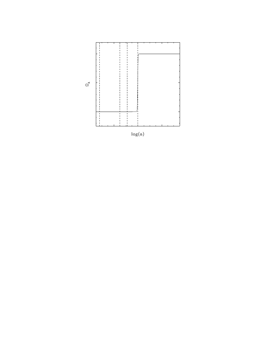
-20
0
20
0
0.5
1
Now
BBN
EW
Planck
Figure 11: Ω
Λ
as a function of the scale factor a, for a universe in which Ω
M0
= 0.3,
Ω
Λ0
= 0.7. Indicated are the scale factors corresponding to the Planck era, the electroweak
phase transition, and Big Bang Nucleosynthesis.
Acknowledgments
I wish to thank Greg Anderson, Tom Banks, Robert Caldwell, Gordon Chalmers, Michael
Dine, George Field, Peter Garnavich, Jeff Harvey, Gordy Kane, Manoj Kaplinghat, Bob Kir-
shner, Lloyd Knox, Finn Larsen, Laura Mersini, Ue-Li Pen, Saul Perlmutter, Joe Polchinski,
Ted Pyne, Brian Schmidt, and Michael Turner for numerous useful conversations, Patrick
Brady, Deryn Fogg and Clifford Johnson for rhetorical encouragement, and Bill Press and
Ed Turner for insinuating me into this formerly-disreputable subject.
References
[1] A. Einstein, Sitz. Preuss. Akad. d. Wiss. Phys.-Math 142 (1917).
[2] E.P. Hubble, Proc. Natl. Acad. Sci. 15, 168 (1929).
[3] S.M. Carroll, W.H. Press, and E.L. Turner, Ann. Rev. Astron. Astrophys. 30, 499
(1992).
[4] J.E. Felten and R. Isaacman, Rev. Mod. Phys. 58, 689 (1986).
[5] J.C. Charlton and M.S. Turner, Astrophys. Journ. 313, 495 (1987).
[6] A. Sandage, Ann. Rev. Astron. Astrophys. 26, 561 (1988).
37
[7] J.D. Cohn, Astrophys. Sp. Sci. 259, 213 (1998) [astro-ph/9807128].
[8] V. Sahni and A. Starobinsky, “The case for a positive cosmological lambda-term,”
[9] M.S. Turner, “Dark matter and dark energy in the universe,” astro-ph/9811454.
[10] S. Weinberg, Rev. Mod. Phys. 61, 1 (1989).
[11] E.W. Kolb and M.S. Turner, The Early Universe (Redwood City, California: Addison-
Wesley, 1990).
[12] A. Linde, Particle Physics and Inflationary Cosmology (New York: Harwood, 1990).
[13] P.J.E. Peebles, Principles of Physical Cosmology (Princeton: Princeton University
Press, 1993).
[14] Y.B. Zel’dovich, Sov. Phys. Uspekhi, 11, 381 (1968).
[15] S.A. Bludman and M.A. Ruderman, Phys. Rev. Lett. 38, 255 (1977).
[16] H. B. Casimir, Kon. Ned. Akad. Wetensch. Proc. 51, 793 (1948).
[17] S.W. Hawking and G.F.R. Ellis, The Large-Scale Structure of Space-Time (Cambridge:
Cambridge University Press, 1973).
[18] M.T. Ressell and M.S. Turner, Comments Astrophys. 14, 323 (1990).
[19] D.J. Fixsen et al., Astrophys. J. 473, 576 (1996).
[20] D. Scott, “Cosmic Glows,” astro-ph/9912038.
[21] A. H. Guth, Phys. Rev. D23, 347 (1981).
[22] A. D. Linde, Phys. Lett. B108, 389 (1982).
[23] A. Albrecht and P. J. Steinhardt, Phys. Rev. Lett. 48, 1220 (1982).
[24] U. Pen, Astrophys. Journ. Supp. 120, 49 (1999) [astro-ph/9904172].
[25] D.J. Heath, Mon. Not. Roy. Astron. Soc. 179, 351 (1977).
[26] D. J. Eisenstein, “An Analytic Expression for the Growth Function in a Flat Universe
with a Cosmological Constant,” astro-ph/9709054.
[27] P. J. Peebles, Astrophys. J. 284, 439 (1984).
[28] M. S. Turner, G. Steigman and L. M. Krauss, Phys. Rev. Lett. 52, 2090 (1984).
38
[29] L. Kofman and A. Starobinsky, Sov. Astron. lett. 11, 271 (1985).
[30] G. Efstathiou, W. J. Sutherland and S. J. Maddox, Nature 348, 705 (1990).
[31] Y. Fujii and T. Nishioka, Phys. Lett. B254, 347 (1991).
[32] L. Kofman, N. Gnedin and N. Bahcall, Astrophys. J. 413, 1 (1993).
[33] L. M. Krauss and M. S. Turner, Gen. Rel. Grav. 27, 1137 (1995) [astro-ph/9504003].
[34] J. P. Ostriker and P. J. Steinhardt, Nature 377, 600 (1995).
[35] M. S. Turner, “The case for Lambda-CDM,” astro-ph/9703161.
[36] D. Branch and G.A. Tammann, Ann. Rev. Astron. Astophys. 30, 359 (1992).
[37] G.A. Tammann, in Astrophysical Uses of the Space Telescope, ed. F.D. Machetto, F.
Pacini, M. Tarenghi, p. 329 (Geneva: ESO, 1979).
[38] A. Goobar and S. Perlmutter, Astrophys. Journ. 450, 14 (1995). [astro-ph/9505022].
[39] S.E. Woosley and T.A. Weaver, Astrophys. Journ. 423, 371 (1994).
[40] I. Hachisu, M. Kato and K. Nomoto, Astrophys. Journ. 522, 487 (1999) [astro-
[41] P. H¨oflich, J.C. Wheeler and F.K. Thielemann, Astrophys.J. 495, 617 (1998) [astro-
[42] M.M. Phillips, Astrophys. J. Lett. 413, L105 (1993).
[43] A.G. Riess, W.H. Press and R.P. Kirshner, Astrophys. Journ. 473, 88 (1996) [astro-
[44] M. Hamuy et al., Astron. Journ. 112, 2438 (1996) [astro-ph/9609059].
[45] H.U. Norgaard-Nielsen, L. Hansen, H.E. Jorgensen, A. Aragon Salamanca, and R.S.
Ellis, Nature, 339, 523 (1989).
[46] P. M. Garnavich et al. [Hi-Z Supernova Team Collaboration], Astrophys. J. 493, L53
(1998) [astro-ph/9710123].
[47] B. P. Schmidt et al. [Hi-Z Supernova Team Collaboration], Astrophys. Journ. 507, 46
(1998) [astro-ph/9805200].
[48] A.G. Riess et al. [Hi-Z Supernova Team Collaboration], Astron. Journ. 116, 1009
(1998) [astro-ph/9805201].
39
[49] P.M. Garnavich et al. [Hi-Z Supernova Team Collaboration], Astrophys. Journ. 509,
74 (1998) [astro-ph/9806396].
[50] S. Perlmutter et al. [Supernova Cosmology Project Collaboration], Astrophys. Journ.
483, 565 (1997) [astro-ph/9608192].
[51] S. Perlmutter et al. [Supernova Cosmology Project Collaboration], Nature 391, 51
(1998) [astro-ph/9712212].
[52] S. Perlmutter et al. [Supernova Cosmology Project Collaboration], Astrophys. Journ.
517, 565 (1999) [astro-ph/9812133].
[53] P. S. Drell, T. J. Loredo and I. Wasserman, Astrophys. Journ. 530, 593 (2000) [astro-
[54] A. G. Riess, A. V. Filippenko, W. Li and B. P. Schmidt, Astron. Journ. 118, 2668
(1999) [astro-ph/9907038].
[55] A. N. Aguirre, Astrophys. Journ. 512, L19 (1999) [astro-ph/9811316].
[56] A. N. Aguirre, Astrophys. Journ. 525, 583 (1999) [astro-ph/9904319].
[57] A. N. Aguirre and Z. Haiman, “Cosmological Constant or Intergalactic Dust? Con-
straints from the Cosmic Far Infrared Background,” astro-ph/9907039.
[58] J.T. Simonsen and S. Hannestad, Astron. Astrophys. 351, 1 (1999); astro-ph/9909225.
[59] T. Totani and C. Kobayashi, Astrophys. Journ. 526, L65 (1999) [astro-ph/9910038].
[60] D. E. Holz and R. M. Wald, Phys. Rev. D58, 063501 (1998) [astro-ph/9708036].
[61] R. Kantowski, Astrophys. Journ. 507, 483 (1998) [astro-ph/9802208].
[63] G.F. Smoot et al., Astrophys. Journ. 396, L1 (1992).
[64] W. Hu, N. Sugiyama and J. Silk, Nature 386, 37 (1997) [astro-ph/9604166].
[65] M. Kamionkowski, D. N. Spergel and N. Sugiyama, Astrophys. Journ. 426, L57 (1994)
[66] G. Jungman, M. Kamionkowski, A. Kosowsky and D. N. Spergel, Phys. Rev. Lett. 76,
1007 (1996) [astro-ph/9507080].
[67] W. Hu and M. White, “Measuring the curvature of the universe,” [astro-ph/9606140].
[68] J. R. Bond, R. Crittenden, R. L. Davis, G. Efstathiou and P. J. Steinhardt, Phys. Rev.
Lett. 72, 13 (1994) [astro-ph/9309041].
40
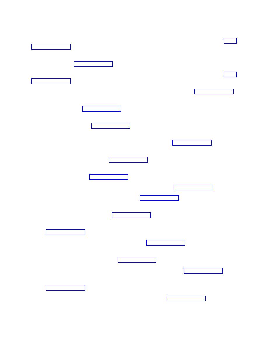
[69] W. Hu, D. Scott, N. Sugiyama and M. White, Phys. Rev. D52, 5498 (1995) [astro-
[70] G. Jungman, M. Kamionkowski, A. Kosowsky and D. N. Spergel, Phys. Rev. D54,
1332 (1996) [astro-ph/9512139].
[71] M. Zaldarriaga, D. N. Spergel and U. Seljak, Astrophys. J. 488, 1 (1997) [astro-
[72] J.R. Bond, A.H. Jaffe and L. Knox, Phys. Rev. D57, 2117 (1998) [astro-ph/9708203].
[73] A. D. Miller et al., “A Measurement of the Angular Power Spectrum of the CMB from
l = 100 to 400,” astro-ph/9906421.
[74] A. Melchiorri et al., “A measurement of Omega from the North American test flight
of BOOMERANG,” astro-ph/9911445.
[75] J. G. Bartlett, A. Blanchard, M. Le Dour, M. Douspis and D. Barbosa, “Constraints
on Cosmological Parameters from Existing CMB Data,” astro-ph/9804158.
[76] C. H. Lineweaver, “The Cosmic Microwave Background and Observational Conver-
gence in the Ω
M
-Ω
Λ
Plane,” astro-ph/9805326.
[77] B. Ratra, R. Stompor, K. Ganga, G. Rocha, N. Sugiyama and K. M. Gorski, Astrophys.
J. 517, 549 (1999) [astro-ph/9901014].
[78] S. Dodelson and L. Knox, “Dark Energy and the CMB,” astro-ph/9909454.
[79] M. White, Astrophys. J. 506, 495 (1998) [astro-ph/9802295].
[80] M. Tegmark, D. J. Eisenstein and W. Hu, “Cosmic complementarity: combining CMB
and supernova observations,” astro-ph/9804168.
[81] W. Hu, D. J. Eisenstein, M. Tegmark and M. White, Phys. Rev. D59, 023512 (1999)
[82] M. Tegmark, Astrophys. J. 514, L69 (1999) [astro-ph/9809201].
[83] G. Efstathiou, S. L. Bridle, A. N. Lasenby, M. P. Hobson and R. S. Ellis, Mon. Not.
Roy. Ast. Soc. 303, L47 (1999) [astro-ph/9812226].
[84] S. L. Bridle et al., Mon. Not. Roy. Ast. Soc. 310, 565 (1999) [astro-ph/9903472].
[85] N. Bahcall, J. P. Ostriker, S. Perlmutter and P. J. Steinhardt, Science 284, 1481 (1999)
[86] J.R. Mould et al., Astrophys. Journ. 529, 698 (2000) [astro-ph/9909269].
41
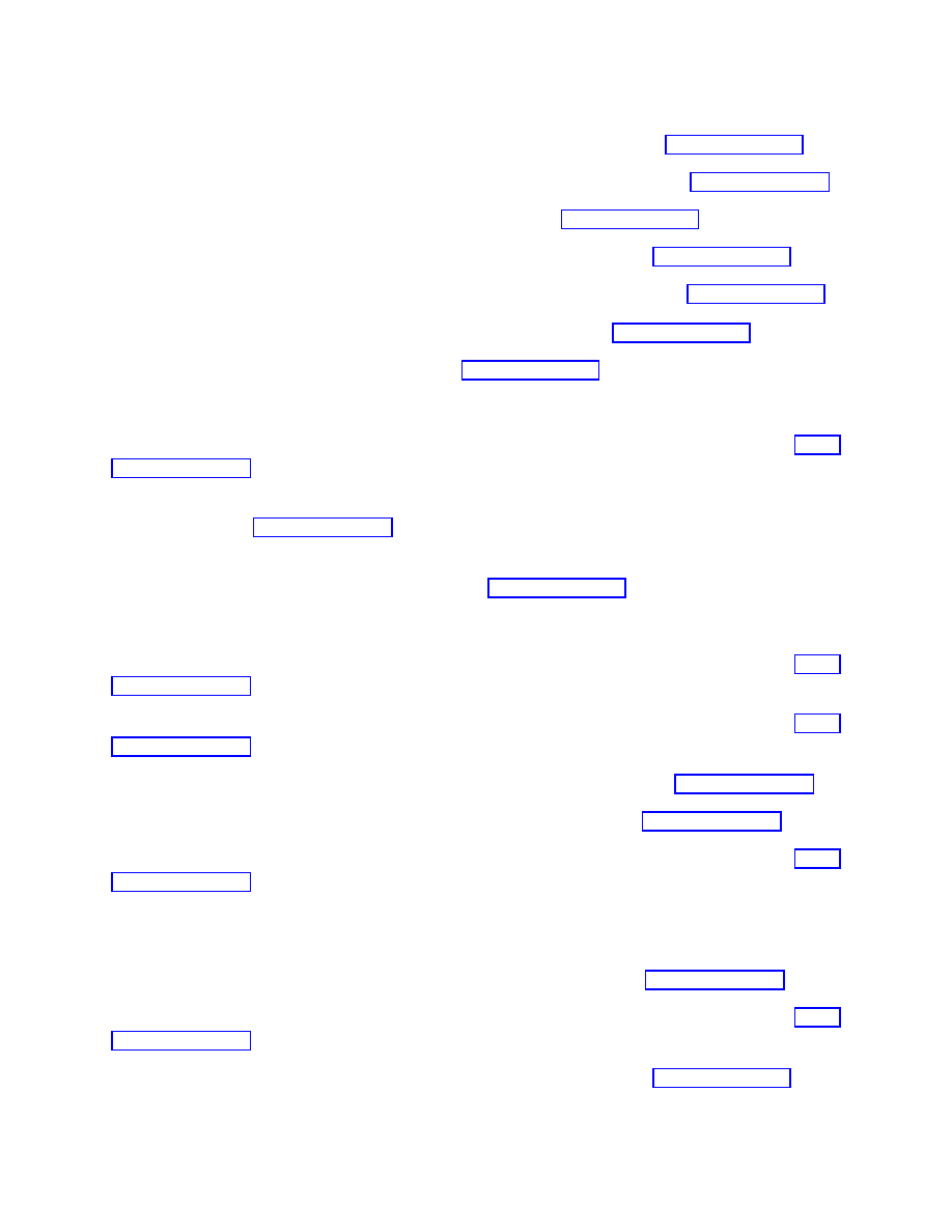
[87] W.L. Freedman, “Determination of Cosmological Parameters”, astro-ph/9905222.
[88] D.N. Schramm and M.S. Turner, Rev. Mod. Phys. 70, 303 (1998) [astro-ph/9706069].
[89] S. Burles et al., Phys. Rev. Lett. 82, 4176 (1999) [astro-ph/9901157].
[90] A. Dekel, D. Burstein and S. D. White, “Measuring Omega,” astro-ph/9611108.
[91] N. A. Bahcall and X. Fan, Publ. Nat. Acad. Sci. 95, 5956 (1998) [astro-ph/9804082].
[92] M.S. Turner, “Dark matter and energy in the universe,” astro-ph/9901109.
[93] J.R. Primack, “Status of cosmology,” astro-ph/9912089.
[94] R.G. Carlberg et al., Astrophys. Journ. 462, 32 (1996).
[95] N. A. Bahcall, L. M. Lubin and V. Dorman, Astrophys. Journ. 447, L81 (1995) [astro-
[96] I. Smail, R.S. Ellis, M.J. Fitchett and A.C. Edge, Mon. Not. Roy. Astron. Soc. 273,
277 (1995) [astro-ph/9402049].
[97] A.D. Lewis, E. Ellingson, S.L. Morris, and R.G. Carlberg, “X-ray Mass Estimates at
z
∼ 0.3 for the CNOC Cluster Sample,” [astro-ph/9901062].
[98] S.D.M. White, J.F. Navarro, A.E. Evrard and C.S. Frenk, Nature 366, 429 (1993).
[99] M. Fukugita, C.J. Hogan and P.J. Peebles, Astrophys. Journ. 503, 518 (1998) [astro-
[100] J. Mohr, B. Mathiesen and G. Evrard, Astrophys. Journ. 517, 627 (1999) [astro-
[101] J. E. Carlstrom et al., “Imaging the Sunyaev-Zel’dovich Effect,” astro-ph/9905255.
[102] N. A. Bahcall and X. Fan, Astrophys. Journ. 504, 1 (1998) [astro-ph/9803277].
[103] N. A. Bahcall, X. Fan, and R. Cen, Astrophys. Journ. 485, L53 (1998) [astro-
[104] R.G. Carlberg, S.L. Morris, H.K.C. Lee, and E. Ellingson, Astrophys. Journ. 479, L19
(1997).
[105] A. Dekel, “Cosmological Implications of Large-Scale Flows,” astro-ph/9705033.
[106] J.A. Peacock and S.J. Dodds, Mon. Not. Roy. Astron. Soc. 267, 1020 (1994) [astro-
[107] D.J. Eisenstein and W. Hu, Astrophys. Journ. 511, 5 (1999) [astro-ph/9710252].
42
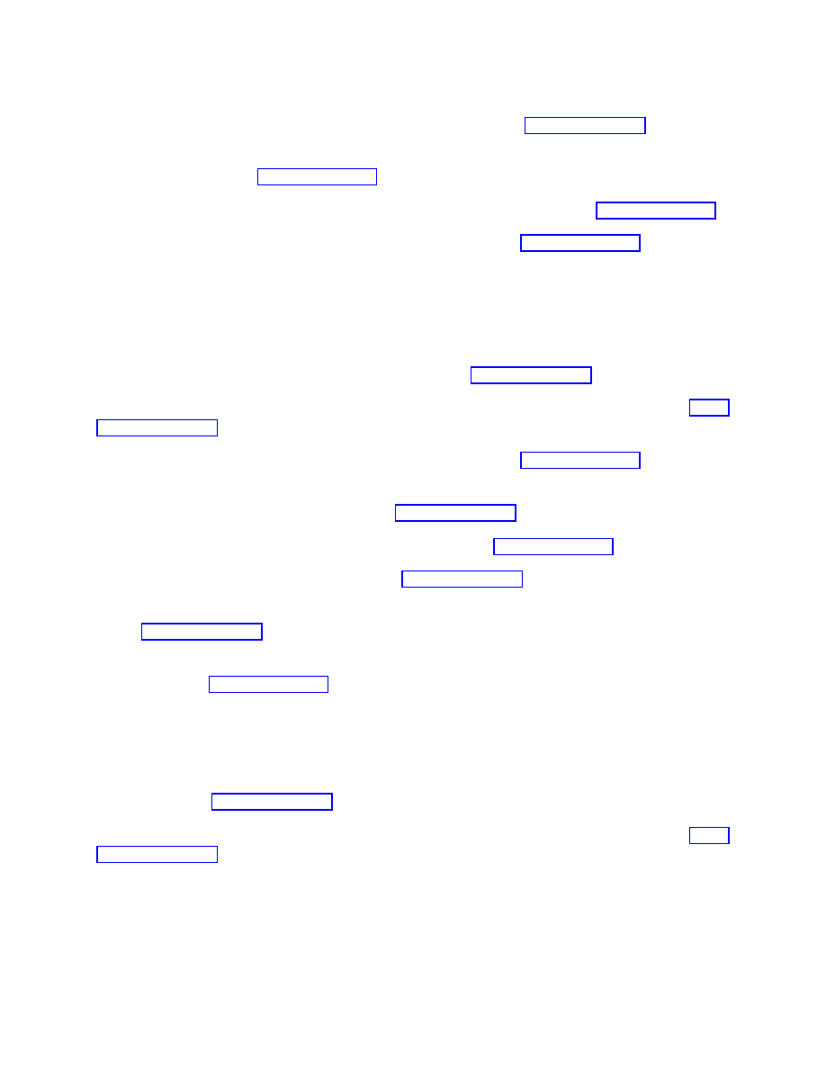
[108] A.R. Liddle and D.H. Lyth, Phys. Rept. 231, 1 (1993) [astro-ph/9303019].
[109] A. R. Liddle, D. H. Lyth, P. T. Viana and M. White, Mon. Not. Roy. Astron. Soc.
282, 281 (1996) [astro-ph/9512102].
[110] S. Dodelson, E.I. Gates and M.S. Turner, Science 274, 69 (1996) [astro-ph/9603081].
[111] J.R. Primack, “Dark matter and structure formation,” astro-ph/9707285.
[112] J.R. Gott, M.G. Park and H.M. Lee, Astrophys. Journ. 338, 1 (1989).
[113] M. Fukugita, T. Futamase and M. Kasai, Mon. Not. Roy. Astron. Soc. 246, 24 (1990).
[114] E. Turner, Astrophys. Journ. 365, L43 (1990).
[115] C. S. Kochanek, Astrophys. J. 466, 638 (1996) [astro-ph/9510077].
[116] E. E. Falco, C. S. Kochanek, J. M. Munoz Astrophys. J. 494, 47 (1996) [astro-
[117] M. Chiba and Y. Yoshii, Astrophys. J. 510, 42 (1999) [astro-ph/9808321].
[118] Y. N. Cheng and L. M. Krauss, “Gravitational lensing statistics and constraints on
the cosmological constant revisited,” astro-ph/9810393.
[119] X. Wu and S. Mao, Astrophys. J. 463, 404 (1996) [astro-ph/9512014].
[120] L. Hui, Astrophys. J. 519, L9 (1999) [astro-ph/9902275].
[121] A. R. Cooray, J. M. Quashnock and M. C. Miller, Astrophys. J. 511, 562 (1999)
[122] J.A. Newman and M. Davis, “Measuring the cosmic equation of state with counts of
galaxies,” astro-ph/9912366.
[123] C. Alcock and B. Paczynski, Nature 281, 358 (1979).
[124] S. Phillips, Mon. Not. Roy. Astron. Soc. 269, 1077 (1994).
[125] P.A. Popowski, D.H. Weinberg, B.S. Ryden, and P.S. Osmer, Astrophys. Journ. 498,
11 (1998) [astro-ph/9707175].
[126] L. Hui, A. Stebbins, and S. Burles, Astrophys. Journ. 511, L5 (1999) [astro-
[127] O. Lahav, P. B. Lilje, J. R. Primack and M. J. Rees, Mon. Not. Roy. Astron. Soc. 251,
128 (1991).
43
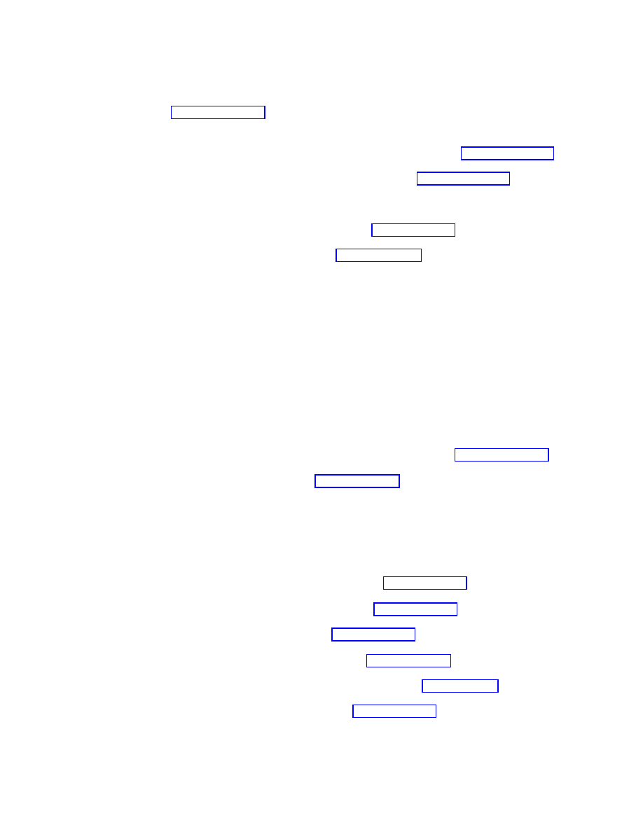
[128] W. E. Ballinger, J. A. Peacock and A. F. Heavens, Mon. Not. Roy. Astron. Soc. 282,
877 (1996) [astro-ph/9605017].
[129] E.J. Guerra, R.A. Daly and L. Wan, “Updated Estimates of Global Cosmological
Parameters Determined Using Classical Double Radio Galaxies,” astro-ph/9807249.
[130] Y. Wang and E. L. Turner, Phys. Rev. D56, 724 (1997) [astro-ph/9603034].
[131] H. P. Nilles, Phys. Rept. 110, 1 (1984).
[132] J. D. Lykken, “Introduction to supersymmetry,” hep-th/9612114.
[133] S. P. Martin, “A supersymmetry primer,” hep-ph/9709356.
[134] B. Zumino, Nucl. Phys. B89, 535 (1975).
[135] E. Cremmer, S. Ferrara, C. Kounnas and D. V. Nanopoulos, Phys. Lett. B133, 61
(1983).
[136] M. Dine and N. Seiberg, Phys. Lett. 162B, 299 (1985).
[137] M. B. Green, J. H. Schwarz and E. Witten, Superstring Theory, two volumes. (Cam-
bridge: Cambridge University Press, 1987).
[138] J. Polchinski, String Theory, two volumes (Cambridge: Cambridge University Press,
1998).
[139] J. D. Lykken, “New and improved superstring phenomenology,” astro-ph/9903026.
[140] T. Banks, “M theory and cosmology,” hep-th/9911067.
[141] G. Moore, Nucl. Phys. B293, 139 (1987).
[142] K. R. Dienes, Phys. Rev. D42, 2004 (1990).
[143] K. R. Dienes, Phys. Rev. Lett. 65, 1979 (1990).
[144] M. Dine, Prog. Theor. Phys. Suppl. 134, 1 (1999) [hep-th/9903212].
[145] E. Witten, Int. J. Mod. Phys. A10, 1247 (1995) [hep-th/9409111].
[146] E. Witten, Nucl. Phys. B443, 85 (1995) [hep-th/9503124].
[147] E. Witten, Mod. Phys. Lett. A10, 2153 (1995) [hep-th/9506101].
[148] G. ’t Hooft, “Dimensional reduction in quantum gravity,” gr-qc/9310026.
[149] L. Susskind, J. Math. Phys. 36, 6377 (1995) [hep-th/9409089].
44
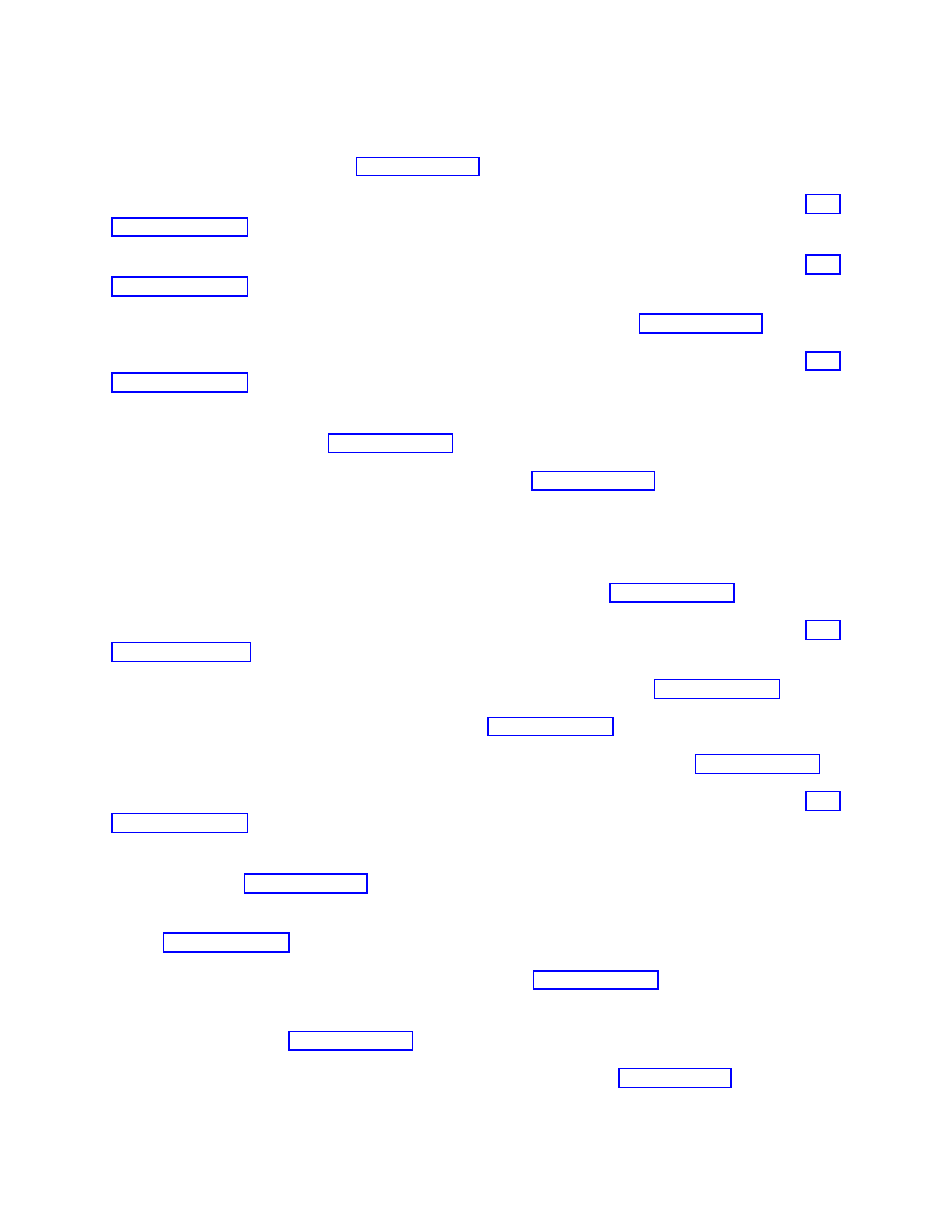
[150] T. Banks, “SUSY Breaking, Cosmology, Vacuum Selection and the Cosmological Con-
stant in String Theory,” hep-th/9601151.
[151] A. G. Cohen, D. B. Kaplan and A. E. Nelson, Phys. Rev. Lett. 82, 4971 (1999) [hep-
[152] E. Verlinde and H. Verlinde, “RG-flow, gravity and the cosmological constant,” hep-
[153] C. Schmidhuber, “AdS
5
and the 4d cosmological constant,” hep-th/9912156.
[154] S. Kachru, J. Kumar and E. Silverstein, Phys. Rev. D59, 106004 (1999) [hep-
[155] R. Iengo and C. Zhu, “Evidence for nonvanishing cosmological constant in non-SUSY
superstring models,” hep-th/9912074.
[156] J.A. Harvey, Phys. Rev. D59, 026002 (1999); [hep-th/9807213].
[157] V.A. Rubakov and M.E. Shaposhnikov, Phys. Lett. 125B, 136 (1983).
[158] I. Antoniadis, Phys. Lett. B246, 377 (1990).
[159] P. Horava and E. Witten, Nucl. Phys. B475, 94 (1996) [hep-th/9603142].
[160] N. Arkani-Hamed, S. Dimopoulos and G. Dvali, Phys. Lett. B429, 263 (1998) [hep-
[161] Z. Kakushadze and S. H. Tye, Nucl. Phys. B548, 180 (1999) [hep-th/9809147].
[162] M. Visser, Phys. Lett. B159, 22 (1985), [hep-th/9910093].
[163] L. Randall and R. Sundrum, “An alternative to compactification,” hep-th/9906064.
[164] M. Gogberashvili, “Gravitational trapping for extended extra dimension,” hep-
[165] P. Binetruy, C. Deffayet and D. Langlois, “Non-conventional cosmology from a brane-
universe,” hep-th/9905012.
[166] P. Kanti, I. I. Kogan, K. A. Olive and M. Pospelov, Phys. Lett. B468, 31 (1999)
[167] P. J. Steinhardt, Phys. Lett. B462, 41 (1999) [hep-th/9907080].
[168] C. P. Burgess, R. C. Myers and F. Quevedo, “A naturally small cosmological constant
on the brane?,” hep-th/9911164.
[169] R. Gambini and J. Pullin, Phys. Lett. B437, 279 (1998) [gr-qc/9803097].
45
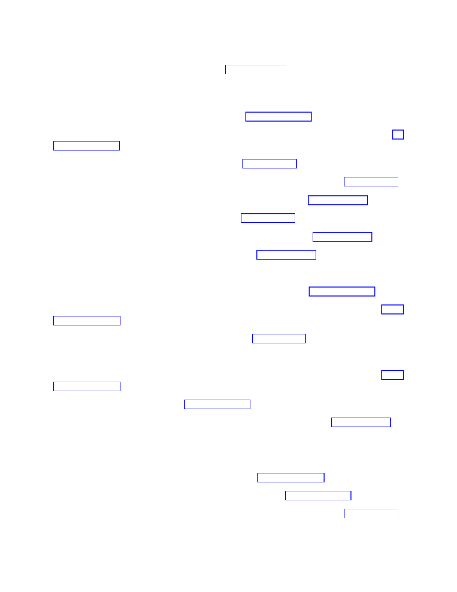
[170] R. Sundrum, JHEP 9907, 001 (1999) [hep-ph/9708329].
[171] J.D. Barrow and F.J. Tipler, The Anthropic Cosmological Principle (Oxford: Claren-
don, 1986).
[172] C. J. Hogan, “Why the universe is just so,” astro-ph/9909295.
[173] A. Linde, “Quantum cosmology and the structure of inflationary universe,” gr-
[174] A. Vilenkin, Phys. Rev. D52, 3365 (1995) [gr-qc/9505031].
[175] A. Linde, D. Linde and A. Mezhlumian, Phys. Rev. D49, 1783 (1994) [gr-qc/9306035].
[176] S. W. Hawking and N. Turok, Phys. Lett. B425, 25 (1998) [hep-th/9802030].
[177] A. Linde, Phys. Rev. D58, 083514 (1998) [gr-qc/9802038].
[178] N. Turok and S. W. Hawking, Phys. Lett. B432, 271 (1998) [hep-th/9803156].
[179] A. Vilenkin, Phys. Rev. Lett. 81, 5501 (1998) [hep-th/9806185].
[180] S. Weinberg, Phys. Rev. Lett. 59, 2607 (1987).
[181] M. Tegmark and M. J. Rees, Astrophys. J. 499, 526 (1998) [astro-ph/9709058].
[182] J. Garriga, M. Livio and A. Vilenkin, Phys. Rev. D61, 023503 (2000) [astro-
[183] A. Vilenkin, Phys. Rev. Lett. 74, 846 (1995) [gr-qc/9406010].
[184] G. Efstathiou, Mon. Not. Roy. Astron. Soc. 274, L73 (1995).
[185] H. Martel, P. R. Shapiro and S. Weinberg, Astrophys. J. 492, 29 (1998) [astro-
[186] J. Garriga and A. Vilenkin, astro-ph/9908115.
[187] T. Banks, M. Dine and N. Seiberg, Phys. Lett. B273, 105 (1991) [hep-th/9109040].
[188] S. Coleman, Nucl. Phys. B310, 643 (1988).
[189] A. D. Dolgov, JETP Lett. 41, 345 (1985).
[190] A. A. Starobinsky, JETP Lett. 68, 757 (1998) [astro-ph/9810431].
[191] S. Weinberg, “Theories of the cosmological constant,” astro-ph/9610044.
[192] E. I. Guendelman and A. B. Kaganovich, Phys. Rev. D55, 5970 (1997) [gr-qc/9611046].
46
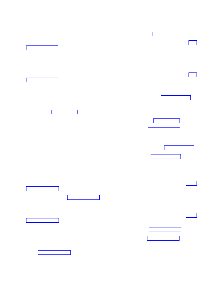
[193] F. Wilczek, Phys. Rev. Lett. 80, 4851 (1998) [hep-th/9801184].
[194] Y. J. Ng and H. van Dam, “A small but nonzero cosmological constant,” hep-
[195] E. T. Tomboulis, Nucl. Phys. B329, 410 (1990).
[196] I. Antoniadis and E. Mottola, Phys. Rev. D45, 2013 (1992).
[197] I. Antoniadis, P. O. Mazur and E. Mottola, Phys. Lett. B444, 284 (1998) [hep-
[198] N. C. Tsamis and R. P. Woodard, Phys. Lett. B301, 351 (1993).
[199] N. C. Tsamis and R. P. Woodard, Nucl. Phys. B474, 235 (1996) [hep-ph/9602315].
[200] L. R. Abramo, R. H. Brandenberger and V. F. Mukhanov, Phys. Rev. D56, 3248
(1997) [gr-qc/9704037].
[201] M. Ozer and M. O. Taha, Mod. Phys. Lett. A13, 571 (1998) [gr-qc/9802023].
[202] W. Unruh, “Cosmological long wavelength perturbations,” astro-ph/9802323.
[203] M. S. Turner and F. Wilczek, Nature 298, 633 (1982).
[204] W. D. Garretson and E. D. Carlson, Phys. Lett. B315, 232 (1993) [hep-ph/9307346].
[205] A. Kusenko and P. Langacker, Phys. Lett. B391, 29 (1997) [hep-ph/9608340].
[206] M. Ozer and M. O. Taha, Nucl. Phys. B287, 776 (1987).
[207] K. Freese, F. C. Adams, J. A. Frieman and E. Mottola, Nucl. Phys. B287, 797 (1987).
[208] J. M. Overduin and F. I. Cooperstock, Phys. Rev. D58, 043506 (1998) [astro-
[209] R. R. Caldwell, astro-ph/9908168.
[210] B. Ratra and A. Quillen, Mon. Not. Roy. Astron. Soc. 259, 738 (1992).
[211] K. Coble, S. Dodelson and J. A. Frieman, Phys. Rev. D55, 1851 (1997) [astro-
[212] M. S. Turner and M. White, Phys. Rev. D56, 4439 (1997) [astro-ph/9701138].
[213] J. A. Frieman and I. Waga, Phys. Rev. D57, 4642 (1998) [astro-ph/9709063].
[214] T. Chiba, N. Sugiyama and T. Nakamura, Mon. Not. Roy. Astron. Soc. 301, 72 (1998)
47
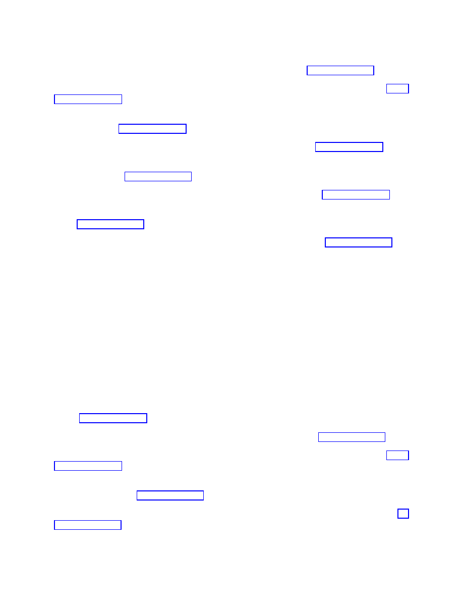
[215] I. Waga and A. P. Miceli, Phys. Rev. D59, 103507 (1999) [astro-ph/9811460].
[216] S. Perlmutter, M. S. Turner and M. White, Phys. Rev. Lett. 83, 670 (1999) [astro-
[217] L. Wang, R. R. Caldwell, J. P. Ostriker and P. J. Steinhardt, Astrophys. Journ. 530,
17 (2000) [astro-ph/9901388].
[218] G. Efstathiou, Mon. Not. Roy. Astron. Soc. 310, 842 (1999) [astro-ph/9904356].
[219] S. Podariu and B. Ratra, “Supernovae Ia constraints on a time-variable cosmological
‘constant’,” astro-ph/9910527.
[220] D. Huterer and M. S. Turner, Phys. Rev. D60, 081301 (1999) [astro-ph/9808133].
[221] A. R. Cooray and D. Huterer, “Gravitational Lensing as a Probe of Quintessence,”
[222] T. D. Saini, S. Raychaudhury, V. Sahni and A. A. Starobinsky, astro-ph/9910231.
[223] A. D. Dolgov, In *Cambridge 1982, Proceedings, The Very Early Universe*, 449-458.
[224] N. Weiss, Phys. Lett. B197, 42 (1987).
[225] P. J. Peebles and B. Ratra, Astrophys. J. 325, L17 (1988).
[226] B. Ratra and P. J. Peebles, Phys. Rev. D37, 3406 (1988).
[227] C. Wetterich, Nucl. Phys. B302, 668 (1988).
[228] C. T. Hill, D. N. Schramm and J. N. Fry, Comments Nucl. Part. Phys. 19, 25 (1989).
[229] Y. Fujii and T. Nishioka, Phys. Rev. D42, 361 (1990).
[230] J. A. Frieman, C. T. Hill and R. Watkins, Phys. Rev. D46, 1226 (1992).
[231] J. A. Frieman, C. T. Hill, A. Stebbins and I. Waga, Phys. Rev. Lett. 75, 2077 (1995)
[232] P. G. Ferreira and M. Joyce, Phys. Rev. D58, 023503 (1998) [astro-ph/9711102].
[233] R. R. Caldwell, R. Dave and P. J. Steinhardt, Phys. Rev. Lett. 80, 1582 (1998) [astro-
[234] G. Huey, L. Wang, R. Dave, R. R. Caldwell and P. J. Steinhardt, Phys. Rev. D59,
063005 (1999) [astro-ph/9804285].
[235] E. J. Copeland, A. R. Liddle and D. Wands, Phys. Rev. D57, 4686 (1998) [gr-
48
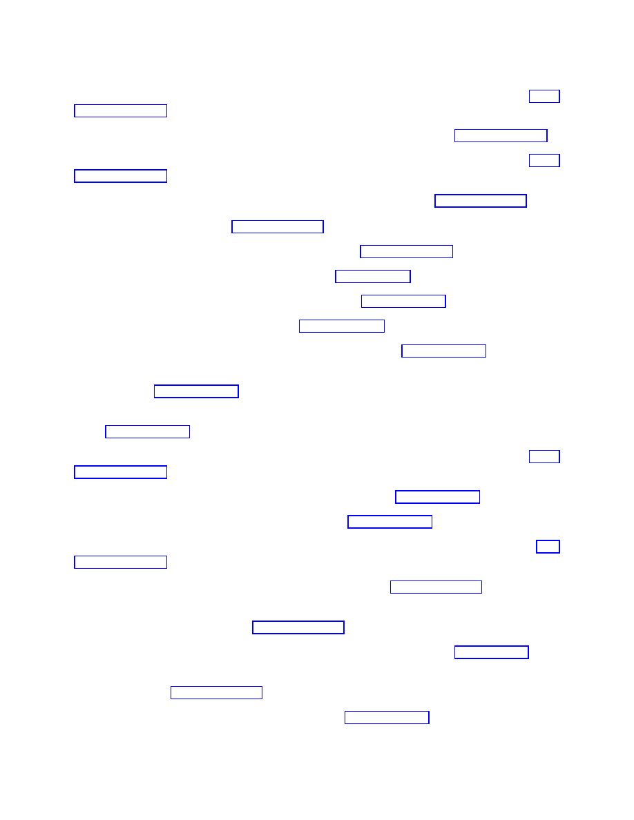
[236] I. Zlatev, L. Wang and P. J. Steinhardt, Phys. Rev. Lett. 82, 896 (1999) [astro-
[237] A. R. Liddle and R. J. Scherrer, Phys. Rev. D59, 023509 (1999) [astro-ph/9809272].
[238] P.J. Steinhardt, L. Wang and I. Zlatev, Phys. Rev. D59, 123504 (1999); [astro-
[239] I. Zlatev and P. J. Steinhardt, Phys. Lett. B459, 570 (1999) [astro-ph/9906481].
[240] V. Sahni and L. Wang, astro-ph/9910097.
[241] S.M. Carroll, Phys. Rev. Lett. 81, 3067 (1998) [astro-ph/9806099].
[242] T. Chiba, Phys. Rev. D60, 083508 (1999) [gr-qc/9903094].
[243] R. Horvat, Mod. Phys. Lett. A14, 2245 (1999) [hep-ph/9904451].
[244] J. E. Kim, JHEP 9905, 022 (1999) [hep-ph/9811509].
[245] K. Choi, “String or M theory axion as a quintessence,” hep-ph/9902292.
[246] J. E. Kim, “Model-dependent axion as quintessence with almost massless hidden sector
quarks,” hep-ph/9907528.
[247] Y. Nomura, T. Watari and T. Yanagida, “Mass generation for an ultralight axion,”
[248] A. Lue, L. Wang and M. Kamionkowski, Phys. Rev. Lett. 83, 1506 (1999) [astro-
[249] C. Kolda and D.H. Lyth, “Quintessential difficulties,” hep-ph/9811375.
[250] P. Binetruy, Phys. Rev. D60, 063502 (1999) [hep-ph/9810553].
[251] A. Masiero, M. Pietroni and F. Rosati, Phys. Rev. D61, 023504 (2000) [hep-
[252] P. Brax and J. Martin, Phys. Lett. B468, 40 (1999) [astro-ph/9905040].
[253] A. Albrecht and C. Skordis, “Phenomenology of a realistic accelerating universe using
only Planck-scale physics,” astro-ph/9908085.
[254] M. C. Bento and O. Bertolami, Gen. Rel. Grav. 31, 1461 (1999) [gr-qc/9905075].
[255] T. Barreiro, E. J. Copeland and N. J. Nunes, “Quintessence arising from exponential
potentials,” astro-ph/9910214.
[256] K. Benakli, Phys. Rev. D60, 104002 (1999) [hep-ph/9809582].
49
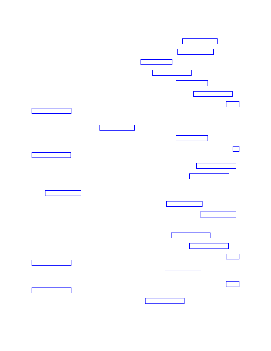
[257] T. Banks, M. Dine and A. Nelson, JHEP 9906, 014 (1999) [hep-th/9903019].
[258] V. Sahni and S. Habib, Phys. Rev. Lett. 81, 1766 (1998) [hep-ph/9808204].
[259] J. Uzan, Phys. Rev. D59, 123510 (1999) [gr-qc/9903004].
[260] L. Amendola, Phys. Rev. D60, 043501 (1999) [astro-ph/9904120].
[261] L. Parker and A. Raval, Phys. Rev. D60, 063512 (1999) [gr-qc/9905031].
[262] F. Perrotta and C. Baccigalupi, Phys. Rev. D59, 123508 (1999) [astro-ph/9811156].
[263] F. Perrotta, C. Baccigalupi and S. Matarrese, Phys. Rev. D61, 023507 (2000) [astro-
[264] R. de Ritis, A. A. Marino, C. Rubano and P. Scudellaro, “Tracker fields from nonmin-
imally coupled theory,” hep-th/9907198.
[265] L. Parker and A. Raval, Phys. Rev. D60, 123502 (1999) [gr-qc/9908013].
[266] O. Bertolami and P. J. Martins, “Non-minimal coupling and quintessence,” gr-
[267] R. A. Frewin and J. E. Lidsey, Int. J. Mod. Phys. D2, 323 (1993) [astro-ph/9312035].
[268] P. J. Peebles and A. Vilenkin, Phys. Rev. D59, 063505 (1999) [astro-ph/9810509].
[269] M. Peloso and F. Rosati, “On the construction of quintessential inflation models,”
[270] M. Giovannini, Class. Quant. Grav. 16, 2905 (1999) [hep-ph/9903263].
[271] G. Felder, L. Kofman and A. Linde, Phys. Rev. D60, 103505 (1999) [hep-ph/9903350].
[272] A. Vilenkin, Phys. Rev. Lett. 53, 1016 (1984).
[273] D. Spergel and U. Pen, Astrophys. J. 491, L67 (1997) [astro-ph/9611198].
[274] M. Bucher and D. N. Spergel, Phys. Rev. D60, 043505 (1999) [astro-ph/9812022].
[275] R. A. Battye, M. Bucher and D. Spergel, “Domain wall dominated universes,” astro-
[276] J. Garcia-Bellido, Int. J. Mod. Phys. D2, 85 (1993) [hep-ph/9205216].
[277] G.W. Anderson and S.M. Carroll, “Dark matter with time-dependent mass”, astro-
[278] W. Hu, Astrophys. Journ. 506, 485 (1998) [astro-ph/9801234].
50
Wyszukiwarka
Podobne podstrony:
open inflation, the four form and the cosmological constant
Physics Papers Andrei Linde (2003), Testing The Cosmological Constant As A Candidate For Dark Energ
Physics Papers Edward Witten (2000), The Cosmological Constant From The Viewpoint Of String Theory
Quantum Symmetry, The Cosmological Constant And Planck Scale Phenomenology
Haisch REPLY TO MICHEL S COMMENT ON ZERO POINT FLUCTUATIONS AND THE COSMOLOGICAL CONSTANT (1997)
astro ph 0102320 LABINI & PIETRONERO Complexity in Cosmology
astro ph 0010634 SIGNORE Supernovae and Cosmology
Klein, Sean [SS] Mr Muerte and the Eyeball Kid [v1 0]
Sean Michael Jarheads Rig and the Gym Bunnies
Sean Michael A Hammer Novel 15 The Two of Swords
Sean Kennedy Chicken Soup for the Soul, And all That Crap
Aspden The Theory of the Proton Constants (1988)
TO THE MOON Constant Vigilance
Aspden The Theory of the Gravitation Constant (1989)
hawking the future of quantum cosmology
Constant current driving of the RGB LED
Millennium's End Terror on the Constantinople
[Mises org]Raico,Ralph The Place of Religion In The Liberal Philosophy of Constant, Toqueville,
więcej podobnych podstron