
Superdiffusions and positive solutions of nonlinear
partial differential equations
E. B. Dynkin
Department of Mathematics, Cornell University, Malott Hall,
Ithaca, New York, 14853


Contents
Preface
v
Chapter 1.
Introduction
1
1.
Trace theory
1
2.
Organizing the book
3
3.
Notation
3
4.
Assumptions
4
5.
Notes
5
Chapter 2.
Analytic approach
7
1.
Operators G
D
and K
D
7
2.
Operator V
D
and equation Lu = ψ(u)
9
3.
Algebraic approach to the equation Lu = ψ(u)
12
4.
Choquet capacities
13
5.
Notes
13
Chapter 3.
Probabilistic approach
15
1.
Diffusion
16
2.
Superprocesses
19
3.
Superdiffusions
23
4.
Notes
28
Chapter 4.
N-measures
29
1.
Main result
29
2.
Construction of measures N
x
30
3.
Applications
33
4.
Notes
39
Chapter 5.
Moments and absolute continuity properties of superdiffusions
41
1.
Recursive moment formulae
41
2.
Diagram description of moments
45
3.
Absolute continuity results
47
4.
Notes
50
Chapter 6.
Poisson capacities
53
1.
Capacities associated with a pair (k, m)
53
2.
Poisson capacities
54
3.
Upper bound for Cap(Γ)
55
4.
Lower bound for Cap
x
59
5.
Notes
61
iii

iv
CONTENTS
Chapter 7.
Basic inequality
63
1.
Main result
63
2.
Two propositions
63
3.
Relations between superdiffusions and conditional diffusions in two open
sets
64
4.
Equations connecting P
x
and N
x
with Π
ν
x
65
5.
Proof of Theorem 1.1
67
6.
Notes
68
Chapter 8.
Solutions w
Γ
are σ-moderate
69
1.
Plan of the chapter
69
2.
Three lemmas on the conditional Brownian motion
70
3.
Proof of Theorem 1.2
71
4.
Proof of Theorem 1.3
73
5.
Proof of Theorem 1.5
73
6.
Proof of Theorems 1.6 and 1.7
75
7.
Notes
75
Chapter 9.
All solutions are σ-moderate
77
1.
Plan
77
2.
Proof of Localization theorem
78
3.
Star domains
81
4.
Notes
87
Appendix A.
An elementary property of the Brownian motion
89
Appendix A.
Relations between Poisson and Bessel capacities
91
Notes
95
References
95
Subject Index
99
Notation Index
101

Preface
This book is devoted to the applications of the probability theory to the theory
of nonlinear partial differential equations. More precisely, we investigate the class
U of all positive solutions of the equation Lu = ψ(u)
in E where L is an elliptic
differential operator of the second order, E is a bounded smooth domain in R
d
and
ψ is a continuously differentiable positive function.
The progress in solving this problem till the beginning of 2002 was described
in the monograph [D]. [We use an abbreviation [D] for [Dyn02].] Under mild
conditions on ψ, a trace on the boundary ∂E was associated with every u ∈ U . This
is a pair (Γ, ν) where Γ is a subset of ∂E and ν is a σ-finite measure on ∂E \ Γ. [A
point y belongs to Γ if ψ
0
(u) tends sufficiently fast to infinity as x → y.] All possible
values of the trace were described and a 1-1 correspondence was established between
these values and a class of solutions called σ-moderate. We say that u is σ-moderate
if it is the limit of an increasing sequence of moderate solutions. [A moderate
solution is a solution u such that u ≤ h where Lh = 0 in E.] In the Epilogue to [D],
a crucial outstanding question was formulated: Are all the solutions σ-moderate?
In the case of the equation ∆u = u
2
in a domain of class C
4
, a positive answer to
this question was given in the thesis of Mselati [Mse02a] - a student of J.-F. Le Gall.
1
However his principal tool - the Brownian snake - is not applicable to more general
equations. In a series of publications by Dynkin and Kuznetsov [Dyn04b], [Dyn04c],
[Dyn04d], [Dyn],[DK03], [DK], [Kuz], Mselati’s result was extended, by using a
superdiffusion instead of the snake, to the equation ∆u = u
α
with 1 < α ≤ 2.
This required an enhancement of the superdiffusion theory which can be of interest
for anybody who works on application of probabilistic methods to mathematical
analysis.
The goal of this book is to give a self-contained presentation of these new
developments. The book may be considered as a continuation of the monograph
[D]. In the first three chapters we give an overview of the theory presented in [D]
without duplicating the proofs which can be found in [D]. The book can be read
independently of [D]. [It might be even useful to read the first three chapters before
reading [D].]
In a series of papers (including [MV98a], [MV98b] and [MV]) M. Marcus and
L. V´
eron investigated positive solutions of the equation ∆u = u
α
by purely analytic
methods. Both, analytic and probabilistic approach have their advantages and an
interaction between analysts and probabilists was important for the progress of the
field. I take this opportunity to thank M. Marcus and L. V´
eron for keeping me
informed about their work.
1
The dissertation of Mselati was published in 2004 (see [Mse04]).
v

vi
PREFACE
I am indebted to S. E. Kuznetsov who provided me several preliminary drafts
of his paper [Kuz] used in Chapters 8 and 9. I am grateful to him and to J.-F. Le
Gall and B. Mselati for many helpful discussions. It is my pleasant duty to thank
J.-F. Le Gall for a permission to include into the book as the Appendix his note
which clarifies a statement used but not proved in Mselati’s thesis (we use it in
Chapter 8).
The Choquet capacities are one of the principal tools in the study of the equa-
tion ∆u = u
α
. This class contains the Poisson capacities used in the work of
Dynkin and Kuznetsov and in this book and the Bessel capacities used by Marcus
and V´
eron and by other analysts. I am very grateful to I. E. Verbitsky who agreed
to write the other Appendix where the relations between the Poisson and Bessel
capacities are established which allow to connect the work of both groups.
I am especially indebted to Yuan-chung Sheu for reading carefully the entire
manuscript and suggesting many corrections and improvements.
The research of the author reported in this book was supported in part by the
National Science Foundation Grant DMS-0204237.

CHAPTER 1
Introduction
1. Trace theory
1.1.
We consider a differential equation
(1.1)
Lu = ψ(u)
in E
where E is a domain in R
d
, L is a uniformly elliptic differential operator in E and
ψ is a function from [0, ∞) to [0, ∞). Under various conditions on E, L and ψ
1
we
investigate the set U of all positive solutions of (1.1). Our base is the trace theory
presented in [D]. Here we give a brief description of this theory (which is applicable
to an arbitrary domain E and a wide class of functions ψ described in Section 4.3).
2
1.2. Moderate and σ-moderate solutions. Our starting point is the rep-
resentation of positive solutions of the linear equation
(1.2)
Lh = 0
in E
by Poisson integrals. If E is smooth
3
and if k(x, y) is the Poisson kernel
4
of L in
E, then the formula
(1.3)
h
ν
(x) =
Z
∂E
k(x, y)ν(dy)
establishes a 1-1 correspondence between the set M(∂E) of all finite measures ν
on ∂E and the set H of all positive solutions of (1.2). (We call solutions of (1.2)
harmonic functions.)
A solution u is called moderate if it is dominated by a harmonic function.
There exists a 1-1 correspondence between the set U
1
of all moderate solutions and
a subset H
1
of H: h ∈ H
1
is the minimal harmonic function dominating u ∈ U
1
,
and u is the maximal solution dominated by h. We put ν ∈ N
1
if h
ν
∈ H
1
. We
denote by u
ν
the element of U
1
corresponding to h
ν
.
An element u of U is called σ-moderate solutions if there exist u
n
∈ U
1
such
that u
n
(x) ↑ u(x) for all x. The labeling of moderate solutions by measures ν ∈ N
1
can be extended to σ-moderate solutions by the convention: if ν
n
∈ N
1
, ν
n
↑ ν and
if u
ν
n
↑ u, then put ν ∈ N
0
and u = u
ν
.
1
We discuss these condtions in Section 4.
2
It is applicable also to functions ψ(x, u) depending on x ∈ E.
3
We use the name smooth for open sets of class C
2,λ
unless another class is indicated
explicitely.
4
For an arbitrary domain, k(x, y) should be replaced by the Martin kernel and ∂E should be
replaced by a certain Borel subset E
0
of the Martin boundary (see Chapter 7 in [D]).
1

2
1. INTRODUCTION
1.3. Lattice structure in U .
5
We write u ≤ v if u(x) ≤ v(x) for all x ∈ E.
This determines a partial order in U . For every ˜
U ⊂ U , there exists a unique
element u of U with the properties: (a) u ≥ v for every v ∈ ˜
U ; (b) if ˜
u ∈ U satisfies
(a), then u ≤ ˜
u. We denote this element Sup ˜
U .
For every u, v ∈ U , we put u ⊕ v = Sup W where W is the set of all w ∈ U
such that w ≤ u + v. Note that u ⊕ v is moderate if u and v are moderate and it
is σ-moderate if so are u and v.
In general, Sup ˜
U does not coincide with the pointwise supremum (the latter
does not belong to U ). However, both are equal if Sup{u, v} ∈ ˜
U for all u, v ∈ ˜
U .
Moreover, in this case there exist u
n
∈ ˜
U such that u
n
(x) ↑ u(x) for all x ∈ E.
Therefore, if ˜
U is closed under ⊕ and it consists of moderate solutions, then Sup ˜
U
is σ-moderate. In particular, to every Borel subset Γ of ∂E there corresponds a
σ-moderate solution
(1.4)
u
Γ
= Sup{u
ν
: ν ∈ N
1
, ν is concentrated on Γ}.
We also associate with Γ another solution w
Γ
. First, we define w
K
for closed
K by the formula
(1.5)
w
K
= Sup{u ∈ U : u = 0
on ∂E \ K}.
For every Borel subset Γ of ∂E, we put
(1.6)
w
Γ
= Sup{w
K
: closed K ⊂ Γ}.
Proving that u
Γ
= w
Γ
was a key part of the program outlined in [D].
1.4. Singular points of a solution u. We consider classical solutions of
(1.1) which are twice continuously differentiable in E. However they can tend to
infinity as x → y ∈ ∂E. We say that y is a singular point of u if it is a point of
rapid growth of ψ
0
(u). [A special role of ψ
0
(u) is due to the fact that the tangent
space to U at point u is described by the equation Lv = ψ
0
(u)v.]
The rapid growth of a positive continuous function a(x) can be defined ana-
lytically or probabilistically. The analytic definition involves the Poisson kernel (or
Martin kernel) k
a
(x, y) of the operator Lu − au: y ∈ ∂E is a point of rapid growth
for a if k
a
(x, y) = 0 for all x ∈ E. A more transparent probabilistic definition is
given in Chapter 3.
We say that a Borel subset Γ of ∂E is f-closed if Γ contains all singular points
of the solution u
Γ
defined by (1.4).
1.5. Definition and properties of trace. The trace of u ∈ U (which we
denote Tr(u)) is defined as a pair (Γ, ν) where Γ is the set of all singular points of
u and ν is a measure on ∂E \ Γ given by the formula
(1.7)
ν(B) = sup{µ(B) : µ ∈ N
1
, µ(Γ) = 0, u
µ
≤ u}.
We have
u
ν
= Sup{ moderate u
µ
≤ u with µ(Γ) = 0}
and therefore u
ν
is σ-moderate.
The trace of every solution u has the following properties:
1.5.A. Γ is a Borel f-closed set; ν is a σ-finite measure of class N
0
such that
ν(Γ) = 0 and all singular points of u
ν
belong to Γ.
5
See Chapter 8, Section 5 in [D].

3. NOTATION
3
1.5.B. If Tr(u) = (Γ, ν), then
(1.8)
u ≥ u
Γ
⊕ u
ν
.
Moreover, u
Γ
⊕ u
ν
is the maximal σ-moderate solution dominated by u.
1.5.C. If (Γ, ν) satisfies the condition 1.5.A, then Tr(u
Γ
⊕ u
ν
) = (Γ
0
, ν), the
symmetric difference between Γ and Γ
0
is not charged by any measure µ ∈ N
1
.
Moreover, u
Γ
⊕ u
ν
is the minimal solution with this property and the only one
which is σ-moderate.
2. Organizing the book
Let u ∈ U and let Tr(u) = (Γ, ν). The proof that u is σ-moderate consists of
three parts:
A. u ≥ u
Γ
⊕ u
ν
.
B. u
Γ
= w
Γ
.
C. u ≤ w
Γ
⊕ u
ν
.
It follows from A–C that u = u
Γ
⊕ u
ν
and therefore u is σ-moderate because
u
Γ
and u
ν
are σ-moderate.
We already have obtained A as a part of the trace theory (see (1.8)) which
covers a general equation (1.1). Parts B and C will be covered for the equation
∆ = u
α
with 1 < α ≤ 2. To this end we use, beside the trace theory, a number
of analytic and probabilistic tools. In Chapters 2 and 3 we survey a part of these
tools (mostly related to the theory of superdiffusion) already prepared in [D]. A
recent enhancement of the superdifusion theory –the N-measures – is presented in
Chapter 4. Another new tool – bounds for the Poisson capacities – is the subject
of Chapter 6. By using all these tools, we prove in Chapter 7 a basic inequality for
superdiffusions which makes it possible to prove (in Chapter 8) that u
Γ
= w
Γ
(Part
B) and therefore w
Γ
is σ-moderate. The concluding part C is proved in Chapter
9 by using absolute continuity results on superdiffusions presented in Chapter 5.
In Chapter 8 we use an upper estimate of w
K
in terms of the Poisson capacity
established by S. E. Kuznetsov [Kuz]. In the Appendix contributed by J.-F. Le
Gall a property of the Brownian motion is proved which is also used in Chapter
8. Notes at the end of each chapter describe the relation of its contents to the
literature on the subject.
3. Notation
3.1.
We use notation C
k
(D) for the set of k times continously differentiable
function on D and we write C(D) for C
0
(D). We put f ∈ C
λ
(D) if there exists a
constant Λ such that |f (x) − f (y)| ≤ Λ|x − y|
λ
for all x, y ∈ D (H¨
older continuity).
Notation C
k,λ
(D) is used for the class of k times differentiable functions with all
partials of order k belonging to C
λ
(D).
We write f ∈ B if f is a positive B-measurable function. Writing f ∈ bB means
that, in addition, f is bounded.
For every subset D of R
d
we denote by B(D) the Borel σ-algebra in D.
We write D b E if ¯
D is a compact subset of E. We say that a sequence D
n
exhausts E if D
1
b D
2
b · · · b D
n
b . . . and E is the union of D
n
.
D
i
stands for the partial derivative
∂
∂x
i
with respect to the coordinate x
i
of x
and D
ij
means D
i
D
j
.

4
1. INTRODUCTION
We denote by M(E) the set of all finite measures on E and by P(E) the set
of all probability measures on E. We write hf, µi for the integral of f with respect
to µ.
δ
y
(B) = 1
B
(y) is the unit mass concentrated at y.
A kernel from a measurable space (E
1
, B
1
) to a measurable space (E
2
, B
2
) is a
function K(x, B) such that K(x, ·) is a finite measure on B
2
for every x ∈ E
1
and
K(·, B) is an B
1
-measurable function for every B ∈ B
2
.
If u is a function on an open set E and if y ∈ ∂E, then writing u(y) = a means
u(x) → a as x → y, x ∈ E.
We put
diam(B) = sup{|x − y| : x, y ∈ B}
(the diameter of B),
d(x, B) = inf
y∈B
|x − y|
(the distance from x to B),
ρ(x) = d(x, ∂E)
for x ∈ E.
We denote by C constants depending only on E, L and ψ (their values can vary
even within one line). We indicate explicitely the dependence on any additional
parameter. For instance, we write C
κ
for a constant depending on a parameter κ
(besides a possible dependence on E, L, ψ).
4. Assumptions
4.1. Operator L. There are several levels of assumptions used in this book.
In the most general setting, we consider a second order differential operator
(4.1)
Lu(x) =
d
X
i,j=1
a
ij
(x)D
ij
u(x) +
d
X
i=1
b
i
(x)D
i
u(x)
in a domain E in R
d
. Without loss of generality we can put a
ij
= a
ji
. We assume
that
4.1.A. [Uniform ellipticity] There exists a constant κ > 0 such that
X
a
ij
(x)t
i
t
j
≥ κ
X
t
2
i
for all x ∈ E, t
1
, . . . , t
d
∈
R.
4.1.B. All coefficients a
ij
(x) and b
i
(x) are bounded and H¨
older continuous.
In a part of the book we assume that L is of divergence form
(4.2)
Lu(x) =
d
X
i,j=1
∂
∂x
i
a
ij
(x)
∂
∂x
j
u(x).
In Chapters 8 and 9 we restrict ourselves to the Laplacian ∆ =
P
d
1
D
2
i
.
4.2. Domain E. Mostly we assume that E is a bounded smooth domain. This
name is used for domains of class C
2,λ
which means that ∂E can be straightened
near every point x ∈ ∂E by a diffeomorphism φ
x
of class C
2,λ
. To define straight-
ening, we consider a half-space E
+
= {x = (x
1
, . . . , x
d
) : x
d
> 0} = R
d−1
× (0, ∞).
Denote E
0
its boundary {x = (x
1
, . . . , x
d
) : x
d
= 0}. We assume that, for every
x ∈ ∂E, there exists a ball B(x, ε) = {y : |x − y| < ε} and a diffeomorphism
φ
x
from B(x, ε) onto a domain ˜
E ⊂ R
d
such that φ
x
(B(x, ε) ∩ E) ⊂ E
+
and

5. NOTES
5
φ
x
(B(x, ε) ∩ ∂E) ⊂ E
0
. (We say that φ
x
straightens the boundary in B(x, ε).) The
Jacobian of φ
x
does not vanish and we can assume that it is strictly positive.
Main results of Chapters 8 and 9 depend on an upper bound for w
K
estab-
lished in [Kuz] for domains of class C
4
. All results of Chapters 8 and 9 can be
automatically extended to domains of class C
2,λ
if the bound for w
K
will be proved
for such domains.
4.3. Function ψ. In general we assume that ψ is a function on [0, ∞) with
the properties:
4.3.A. ψ ∈ C
2
(R
+
).
4.3.B. ψ(0) = ψ
0
(0) = 0, ψ
00
(u) > 0 for u > 0.
[It follows from 4.3.B that ψ is monotone and convex and ψ
0
is bounded on
each interval [0, t].]
4.3.C. There is a constant a such that
ψ(2u) ≤ aψ(u)
for all u.
4.3.D.
R
∞
N
ds
R
s
0
ψ(u) du
−1/2
< ∞ for some N > 0.
Keller [Kel57] and Osserman [Oss57] proved independently that this condition im-
plies that functions u ∈ U (E) are uniformly bounded on every set D b E.
6
In Chapters 7-9 we assume that
(4.3)
ψ(u) = u
α
, 1 < α ≤ 2.
(In Chapter 6 we do not need the restriction α ≤ 2.)
5. Notes
The trace Tr(u) was introduced in [Kuz98] and [DK98b] under the name the
fine trace. We suggested to use the name ”rough trace“ for a version of the trace
considered before in the literature. (In the monograph [D] the rough trace is treated
in Chapter 10 and the fine trace is introduced and studied in Chapter 11.)
The most publications were devoted to the equation
(5.1)
∆u = u
α
, α > 1.
In the subcritical case 1 < d <
α+1
α−1
, the rough trace coincides with the fine trace
and it determines a solution of (5.1) uniquely. As it was shown by Le Gall, this is
not true in the supercritical case: d ≥
α+1
α−1
.
In a pioneering paper [GV91] Gmira and V´
eron proved that, in the subcritical
case, the generalized Dirichlet problem
∆u = u
α
in E,
u = µ
on ∂E
(5.2)
has a unique solution for every finite measure µ. (In our notation, this is u
µ
.)
A program of investigating U by using a superdiffusion was initiated in [Dyn91a].
In [Dyn94] Dynkin conjectured that, for every 1 < α ≤ 2 and every d, the problem
(5.2) has a solution if and only if µ does not charge sets which are, a.s., not hit
6
In a more general setting this is proved in [D], Section 5.3.

6
1. INTRODUCTION
by the range of the superdiffusion.
7
[The conjecture was proved, first, in the case
α = 2, by Le Gall and then, for all 1 < α ≤ 2, by Dynkin and Kuznetsov .]
A classification of all positive solutions of ∆u = u
2
in the unit disk E = {x ∈
R
2
: |x| < 1} was announced by Le Gall in [LG93]. [This is also a subcritical case.]
The result was proved and extended to a wide class of smooth planar domains in
[LG97]. Instead of a superdiffusion Le Gall used his own invention – a path-valued
process called the Brownian snake. He established a 1-1 correspondence between
U and pairs (Γ, ν) where Γ is a closed subset of ∂E and ν is a Radon measure on
∂E \ Γ.
Dynkin and Kuznetsov [DK98a] extended Le Gall’s results to the equation
Lu = u
α
, 1 < α ≤ 2. They introduced a rough boundary trace for solutions of this
equation. They described all possible values of the trace and they represented the
maximal solution with a given trace in terms of a superdiffusion.
Marcus and V´
eron [MV98a]–[MV98b] investigated the rough traces of solutions
by purely analytic means. They extended the theory to the case α > 2 and they
proved that the rough trace determines a solution uniquely in the subcritical case.
The theory of fine trace developed in [DK98b] provided a classification of all
σ-moderate soltions. Mselati’s dissertation [Mse02a] finalized the classification for
the equation ∆u = u
2
by demonstrating that, in this case, all solutions are σ-
moderate. A substantial enhancement of the superdiffusion theory was necessary
to get similar results for a more general equation ∆u = u
α
with 1 < α ≤ 2.
7
The restriction α ≤ 2 is needed because a related superdiffusion exists only in this range.

CHAPTER 2
Analytic approach
In this chapter we consider equation 1.(1.1) under minimal assumptions on L, ψ
and E: conditions 1.4.1.A– 1.4.1.B for L, conditions 1.4.3.A–1.4.3.D for ψ and and
assumption that E is bounded and belongs to class C
2,λ
.
For every open subset D of E we define an operator V
D
that maps positive
Borel functions on ∂D to positive solutions of the equation Lu = ψ(u) in D. If
D is smooth and f is continuous, then V
D
(f ) is a solution of the boundary value
problem
Lu = ψ(u)
in D,
u = f
on ∂D.
In general, u = V
D
(f ) is a solution of the integral equation
u + G
D
ψ(u) = K
D
f
where G
D
and K
D
are the Green and Poisson operators for L in D. Operators V
D
have the properties:
V
D
(f ) ≤ V
D
( ˜
f )
if f ≤ ˜
f ,
V
D
(f
n
) ↑ V
D
(f )
if f
n
↑ f,
V
D
(f
1
+ f
2
) ≤ V
D
(f
1
) + V
D
(f
2
).
The Comparison principle plays for the equation 1.(1.1) a role similar to the
role of the Maximum principle for linear elliptic equations. There is also an analog
of the Mean value property: if u ∈ U (E), then V
D
(u) = u for every D b E. The set
U (E) of all positive solutions is closed under Sup and under pointwise convergence.
We label moderate solutions by measures ν on ∂E belonging to a class N
E
1
and we label σ-moderate solutions by a wider class N
E
0
. A special role is played by
ν ∈ N
E
0
taking only values 0 and ∞.
An algebraic approach to the equation 1.(1.1) is discussed in Section 3. In Sec-
tion 4 we introduce the Choquet capacities which play a crucial role in subsequent
chapters.
Most propositions stated in Chapters 2 and 3 are proved in [D]. In each case we
give an exact reference to the corresponding place in [D]. We provide a complete
proof for every statement not proved in [D].
1. Operators G
D
and K
D
1.1. Green function and Green operator. Suppose that D is a bounded
smooth domain and that L satisfies conditions 1.4.1.A–1.4.1.B. Then there exists a
7

8
2. ANALYTIC APPROACH
unique continuous function g
D
from ¯
D × ¯
D to [0, ∞] such that, for every f ∈ C
λ
(D),
(1.1)
u(x) =
Z
D
g
D
(x, y)f (y)dy
is the unique solution of the problem
Lu = −f
in D,
u = 0
on ∂D.
(1.2)
The function g
D
is called the Green function. It has the following properties:
1.1.A. For every y ∈ D, u(x) = g
D
(x, y) is a solution of the problem
Lu = 0
in D \ {y},
u = 0
on ∂D.
(1.3)
1.1.B. For all x, y ∈ D,
(1.4)
0 < g
D
(x, y) ≤ CΓ(x − y)
where C is a constant depending only on D and L and
1
(1.5)
Γ(x) =
|x|
2−d
for d ≥ 3,
(− log |x|) ∨ 1
for d = 2,
1
for d = 1.
If L is of divergence form and d ≥ 3, then
(1.6)
g
D
(x, y) ≤ Cρ(x)|x − y|
1−d
,
(1.7)
g
D
(x, y) ≤ Cρ(x)ρ(y)|x − y|
−d
.
[See [GW82].]
The Green operator is defined by the formula (1.1).
1.2. Poisson kernel and Poisson operator. Suppose that D is a bounded
smooth domain and let γ be the surface area on ∂D. The Poisson kernel k
D
is a
continuous function from D × ∂D to (0, ∞) with the property: for every ϕ ∈ C(D),
(1.8)
h(x) =
Z
∂D
k
D
(x, y)ϕ(y)γ(dy)
is a unique solution of the problem
Lu = 0
in D,
u = ϕ
on ∂D.
(1.9)
We have the following bounds for the Poisson kernel:
2
(1.10)
C
−1
ρ(x)|x − y|
−d
≤ k
D
(x, y) ≤ Cρ(x)|x − y|
−d
where
(1.11)
ρ(x) = dist(x, ∂D).
The Poisson operator K
D
is defined by the formula (1.8).
1
There is a misprint in the expression for Γ(x) in [D], page 88.
2
See, e.g. [MVG75], Lemma 6 and the Appendix B in [D].

2. OPERATOR V
D
AND EQUATION Lu = ψ(u)
9
2. Operator V
D
and equation Lu = ψ(u)
2.1. Operator V
D
. By Theorem 4.3.1 in [D], if ψ satisfies conditions 1.4.3.B
and 1.4.3.C, then, for every f ∈ bB( ¯
E) and for every open subset D of E, there
exists a unique solution of the equation
(2.1)
u + G
D
ψ(u) = K
D
f.
We denote it V
D
(f ). It follows from (2.1) that:
2.1.A. V
D
(f ) ≤ K
D
(f ), in particular, V
D
(c) ≤ c for every constant c.
We have:
2.1.B. [[D], 4.3.2.A] If f ≤ ˜
f , then V
D
(f ) ≤ V
D
( ˜
f ).
2.1.C. [[D], 4.3.2.C] If f
n
↑ f , then V
D
(f
n
) ↑ V
D
(f ).
Properties 2.1.B and 2.1.C allow to define V
D
(f ) for all f ∈ B( ¯
D) by the
formula
(2.2)
V
D
(f ) = sup
n
V
D
(f ∧ n).
The extended operators satisfy equation (2.1) and conditions 2.1.A-2.1.C. They
have the properties:
2.1.D. [[D], Theorem 8.2.1] For every f
1
, f
2
∈ B(D),
(2.3)
V
D
(f
1
+ f
2
) ≤ V
D
(f
1
) + V
D
(f
2
).
2.1.E. [[D], 8.2.1.J] For every D and every f ∈ B(∂D), the function u = V
D
(f )
is a solution of the equation
(2.4)
Lu = ψ(u)
in D.
We denote by U (D) the set of all positive solutions of the equation (2.4).
2.2. Properties of U (D). We have:
2.2.A. [[D], 8.2.1.J and 8.2.1.H] If D is smooth and if f is continuous in a
neighborhood O of ˜
x ∈ ∂D, then V
D
f (x) → f (˜
x) at x → ˜
x, x ∈ D. If D is smooth
and bounded and if a function f : ∂D → [0, ∞) is continuous, then u = V
D
(f ) is a
unique solution of the problem
Lu = ψ(u)
in D,
u =f
on ∂D.
(2.5)
2.2.B. (Comparison principle)[[D], 8.2.1.H.] Suppose D is bounded. Then u ≤ v
assuming that u, v ∈ C
2
(D),
(2.6)
Lu − ψ(u) ≥ Lv − ψ(v)
in D
and, for every ˜
x ∈ ∂D,
(2.7)
lim sup[u(x) − v(x)] ≤ 0
as x → ˜
x.
2.2.C. (Mean value property)[[D], 8.2.1.D] If u ∈ U (D), then, for every U b D,
V
U
(u) = u in D (which is equivalent to the condition u + G
U
ψ(u) = K
U
u).

10
2. ANALYTIC APPROACH
2.2.D. [[D], Theorem 5.3.2] If u
n
∈ U (E) converge pointwise to u, then u belongs
to U (E).
2.2.E. [[D], Theorem 5.3.1] For every pair D b E there exists a constant b such
that u(x) ≤ b for all u ∈ U (E) and all x ∈ D.
3
The next two propositions are immediate implications of the Comparison prin-
ciple.
We say that u ∈ C
2
(E) is a supersolution if Lu ≤ ψ(u) in E and that it is
a subsolution if Lu ≥ ψ(u) in E. Every h ∈ H(E) is a supersolution because
Lh = 0 ≤ ψ(h). It follows from 2.2.B that:
2.2.F. If a subsolution u and a supersolution v satisfy (2.7), then u ≤ v in E.
2.2.G. If ψ(u) = u
α
with α > 1, then, for every u ∈ U (D) and for all x ∈ D,
u(x) ≤ Cd(x, ∂D)
−2/(α−1)
.
Indeed, if d(x, ∂D) = ρ, then the ball B = {y : |y − x| < ρ} is contained
in D. Function v(y) = C(ρ
2
− |y − x|
2
)
−2/(α−1)
is equal to ∞ on ∂B and, for
sufficiently large C, Lv(y) − v(y)
α
≤ 0 in B.
4
By 2.2.B, u ≤ v in B. In particular,
u(x) ≤ v(x) = Cρ
−2/(α−1)
.
2.3. On moderate solutions. Recall that an element u of U (E) is called
moderate if u ≤ h for some h ∈ H(E). The formula
(2.8)
u + G
E
ψ(u) = h
establishes a 1-1 correspondence between the set U
1
(E) of moderate elements of
U (E) and a subset H
1
(E) of H(E): h is the minimal harmonic function dominating
u, and u is the maximal solution dominated by h. Formula 1.(1.3) defines a 1-1
correspondence ν ↔ h
ν
between M(∂E) and H(E). We put ν ∈ N
E
1
if h
ν
∈ H
1
(E)
and we denote u
ν
the moderate solution corresponding to ν ∈ N
E
1
. In this notation,
(2.9)
u
ν
+ G
E
ψ(u
ν
) = h
ν
.
(The correspondence ν ↔ u
ν
is 1-1 and monotonic.)
We need the following properties of N
E
1
, H
1
(E) and U
1
(E).
2.3.A. [Corollary 3.1 in [D], Section 8.3.2] If h ∈ H
1
(E) and if h
0
≤ h belongs
to H(E), then h
0
∈ H
1
(E). Therefore N
E
1
contains with ν all measures ν
0
≤ ν.
2.3.B. [[D],Theorem 8.3.3] H
1
(E) is a convex cone (that is it is closed under
addition and under multiplication by positive numbers).
2.3.C. If Γ is a closed subset of ∂E and if ν ∈ M(E) is concentrated on Γ, then
h
ν
= 0 on ∂E \ Γ.
Indeed, it follows from 1.(1.3) and (1.10) that
h
ν
(x) ≤ Cρ(x)
Z
Γ
|x − y|
−d
ν(dy).
2.3.D. If ν ∈ N
E
1
and Γ is a closed subset of ∂E, then u
ν
= 0 on O = ∂E \ Γ if
and only if ν(O) = 0.
3
As we already have mentioned, this is an implication of 1.4.3.D.
4
See, e.g., [Dyn91a], page 102, or [D], page 71.

2. OPERATOR V
D
AND EQUATION Lu = ψ(u)
11
Proof. If ν(O) = 0, then h
ν
= 0 on O by 2.3.C, and u
ν
= 0 on O because
u
ν
≤ h
ν
by (2.8).
On the other hand, if u
ν
= 0 on O, then ν(K) = 0 for every closed subset K of
O. Indeed, if η is the restriction of ν to K, then u
η
= 0 on Γ because Γ ⊂ ∂E \ K
and η(∂E \ K) = 0. We also have u
η
≤ u
ν
= 0 on O. Hence u
η
= 0 on ∂E. The
Comparison principle 2.2.B implies that u
η
= 0. Therefore η = 0.
2.3.E. [[D], Proposition 12.2.1.A]
5
If h ∈ H(E) and if G
E
ψ(h)(x) < ∞ for
some x ∈ E, then h ∈ H
1
(E).
2.3.F. (Extended mean value property) If U ⊂ D and if ν ∈ N
D
1
is concentrated
on Γ such that ¯
Γ ∩ ¯
U = ∅, then V
U
(u
ν
) = u
ν
.
If u ∈ U
1
(D) vanishes on ∂D \ Γ, then V
U
(u) = u for every U ⊂ D such that
¯
Γ ∩ ¯
U = ∅.
The first part is Theorem 8.4.1 in [D]. The second part follows from the first one
because u ∈ U
1
(D) is equal to u
ν
for some ν ∈ N
D
1
and, by 2.3.D, ν(∂D \ ¯
Γ) = 0.
2.3.G. Suppose that ν ∈ N
E
1
is supported by a closed set K ⊂ ∂E and let
E
ε
= {x ∈ E : d(x, K) > ε}. Then
u
ε
= V
E
ε
(h
ν
) ↓ u
ν
as ε ↓ 0.
Proof. Put V
ε
= V
E
ε
. By (2.9), h
ν
= u
ε
+ G
E
ε
ψ(u
ε
) ≥ u
ε
for every ε. Let
ε
0
< ε. By applying the second part of 2.3.F to U = E
ε
, D = E
ε
0
, u = u
ε
0
and
Γ = ∂E
ε
0
∩ E we get V
ε
(u
ε
0
) = u
ε
0
. By 2.1.B,
u
ε
= V
ε
(h
ν
) ≥ V
ε
(u
ε
0
) = u
ε
0
.
Hence u
ε
tends to a limit u as ε ↓ 0. By 2.2.D, u ∈ U (E). For every ε, u
ε
≤ h
ν
and therefore u ≤ h
ν
. On the other hand, if v ∈ U (E) and v ≤ h
ν
, then, by 2.3.F,
v = V
ε
(v) ≤ V
ε
(h
ν
) = u
ε
and therefore v ≤ u. Hence, u is a maximal element of
U (E) dominated by h
ν
which means that u = u
ν
.
2.4. On σ-moderate solutions. Denote by U
0
(E) the set of all σ-moderate
solutions. (Recall that u is σ-moderate if there exist moderate u
n
such that u
n
↑ u.)
If ν
1
≤ · · · ≤ ν
n
≤ . . . is an increasing sequence of measures, then ν = lim ν
n
is also
a measure. We put ν ∈ N
E
0
if ν
n
∈ N
E
1
. If ν ∈ N
E
1
, then ∞ · ν = lim
t↑∞
tν belongs to
N
E
0
. Measures µ = ∞ · ν take only values 0 and ∞ and therefore cµ = µ for every
0 < c ≤ ∞. [We put 0 · ∞ = 0.]
Lemma 2.1. [[D], Lemma 8.5.1] There exists a monotone mapping ν → u
ν
from N
E
0
onto U
0
(E) such that
(2.10)
u
ν
n
↑ u
ν
if ν
n
↑ ν
and, for ν ∈ N
E
1
, u
ν
is the maximal solution dominated by h
ν
The following properties of N
E
0
are proved on pages 120-121 of [D]:
2.4.A. A measure ν ∈ N
E
0
belongs to N
E
1
if and only if ν(E) < ∞. If ν
n
∈ N
1
(E)
and ν
n
↑ ν ∈ M(∂E), then ν ∈ N
E
1
.
6
5
Proposition 12.2.1.A is stated for ψ(u) = u
α
but the proof is applicable to a general ψ.
6
See [D]. 8.5.4.A.

12
2. ANALYTIC APPROACH
2.4.B. If ν ∈ N
E
0
and if µ ≤ ν, then µ ∈ N
E
0
.
2.4.C. Suppose E is a bounded smooth domain and O is a relatively open subset
of ∂E. If ν ∈ N
E
0
and ν(O) = 0, then u
ν
= 0 on O.
An important class of σ-moderate solutions are u
Γ
defined by 1.(1.4).
2.4.D. [[D], 8.5.5.A] For every Borel Γ ⊂ ∂E, there exists ν ∈ N
E
1
concentrated
on Γ such that u
Γ
= u
∞·ν
.
2.5. On solution w
Γ
. We list some properties of these solutions (defined in
the Introduction by (1.5) and (1.6)).
2.5.A. [[D], Theorem 5.5.3] If K is a closed subset of ∂E, then w
K
defined by
1.(1.5) vanishes on ∂E \ K. [It is the maximal element of U (E) with this property.]
2.5.B. If ν ∈ N
E
0
is concentrated on a Borel set Γ, then u
ν
≤ w
Γ
.
Proof. If ν ∈ N
E
1
is supported by a compact set K, then u
ν
= 0 on ∂E \ K
by 2.4.C and u
ν
≤ w
K
by 1.(1.5). If ν ∈ N
E
0
, then there exist ν
n
∈ N
E
1
such that
ν
n
↑ ν. The measures ν
n
are also concentrated on Γ and therefore there exists a
sequence of compact sets K
mn
⊂ Γ such that ν
mn
↑ ν
n
where ν
mn
is the restriction
of ν
n
to K
mn
. We have u
ν
mn
≤ w
K
mn
≤ w
Γ
. Hence, u
ν
≤ w
Γ
.
3. Algebraic approach to the equation Lu = ψ(u)
In the Introduction we defined, for every subset ˜
U of U (E), an element Sup ˜
U
of U (E) and we introduced in U (E) a semi-group operation u ⊕ v. In a similar way,
we define now Inf ˜
U as the maximal element u of U (E) such that u ≤ v for all
v ∈ ˜
U . We put, for u, v ∈ U such that u ≥ v,
u v = Inf{w ∈ U : w ≥ u − v}.
Both operations ⊕ and can be expressed through an operator π.
Denote by C
+
(E) the class of all positive functions f ∈ C(E). Put u ∈ D(π)
and π(u) = v if u ∈ C
+
(E) and V
D
n
(u) → v pointwise for every sequence D
n
exhausting E.
By 2.1.E and 2.2.D, π(u) ∈ U (E).
It follows from 2.1.B that
π(u
1
) ≤ π(u
2
) if u
1
≤ u
2
.
Put
U
−
(E) = {u ∈ C
+
(E) : V
D
(u) ≤ u
for all D b E}
and
U
+
(E) = {u ∈ C
+
(E) : V
D
(u) ≥ u
for all D b E}.
By 2.2.C, U (E) ⊂ U
−
(E) ∩ U
+
(E). It follows from the Comparison principle 2.2.B
that U
−
contains all supersolutions and U
+
contains all subsolutions. In particular,
H(E) ⊂ U
−
(E).
For every sequence D
n
exhausting E, we have: [see [D], 8.5.1.A–8.5.1.D]
3.A. If u ∈ U
−
(E), then V
D
n
(u) ↓ π(u) and
π(u) = sup{˜
u ∈ U (E) : ˜
u ≤ u} ≤ u.
3.B. If u ∈ U
+
(E), then V
D
n
(u) ↑ π(u) and
π(u) = inf{˜
u ∈ U (E) : ˜
u ≥ u} ≥ u.
Clearly,

5. NOTES
13
3.C. If u, v ∈ U
+
(E), then max{u, v} ∈ U
+
(E).
If u, v ∈ U
−
(E), then
min{u, v} ∈ U
−
(E).
It follows from 2.1.D (subadditivity of V
D
) that:
3.D. If u, v ∈ U
−
(E), then u + v ∈ U
−
(E). If u, v ∈ U (E) and u ≥ v, then
u − v ∈ U
+
(E).
It is easy to see that:
3.E. If u, v ∈ U (E), then u ⊕ v = π(u + v)
3.F. If u ≥ v ∈ U (E), then u v = π(u − v).
Denote U
∗
(E) the minimal convex cone that contains U
−
(E) and U
+
(E).
4. Choquet capacities
Suppose that E is a separable locally compact metrizable space. Denote by K
the class of all compact sets and by O the class of all open sets in E. A [0, +∞]-
valued function Cap on the collection of all subsets of E is called a capacity if:
4.A. Cap(A) ≤ Cap(B) if A ⊂ B.
4.B. Cap(A
n
) ↑ Cap(A) if A
n
↑ A.
4.C. Cap(K
n
) ↓ Cap(K) if K
n
↓ K and K
n
∈ K.
A set B is called capacitable if These conditions imply
(4.1) Cap(B) = sup{Cap(K) : K ⊂ B, K ∈ K} = inf{Cap(O) : O ⊃ B, O ∈ O}.
The following results are due to Choquet [Cho53].
I. Every Borel set B is capacitable.
7
II. Suppose that a function Cap : K → [0, +∞] satisfies 4.A–4.C and the
following condition:
4.D. For every K
1
, K
2
∈ K,
Cap(K
1
∪ K
2
) + Cap(K
1
∩ K
2
) ≤ Cap(K
1
) + Cap(K
2
).
Then Cap can be extended to a capacity on E.
5. Notes
The class of moderate solutions was introduced and studied in [DK96a]. σ-
moderate solutions, the lattice structure in the space of solutions and the operation
u ⊕ v apeared, first, in [DK98b] in connection with the fine trace theory. The
operation u v was defined and used by Mselati in [Mse02a].
7
The relation (4.1) is true for a larger class of analytic sets but we do not use this fact.


CHAPTER 3
Probabilistic approach
Our base is the theory of diffusions and superdiffusions.
A diffusion describes a random motion of a particle. An example is the Brow-
nian motion in R
d
. This is a Markov process with continuous paths and with the
transition density
p
t
(x, y) = (2πt)
−d/2
e
−|x−y|
2
/2t
which is the fundamental solution of the heat equation
∂u
∂t
=
1
2
∆u.
A Brownian motion in a domain E can be obtained by killing the path at the first
exit time from E. By replacing
1
2
∆ by an operator L of the form 1.(4.1), we define
a Markov process called L-diffusion. We also use an L-diffusion with killing rate `
corresponding to the equation
∂u
∂t
= Lu − `u
and an L-diffusion conditioned to exit from E at a point y ∈ ∂E. The latter can
be constructed by the so-called h-transform with h(x) = k
E
(x, y).
An (L, ψ)-superdiffusion is a model of random evolution of a cloud of particles.
Each particle performs an L-diffusion. It dies at random time leaving a random
offspring of the size regulated by the function ψ. All children move independently
of each other (and of the family history) with the same transition and procreation
mechanism as the parent. Our subject is the family of the exit measures (X
D
, P
µ
)
from open sets D ⊂ E. An idea of this construction is explained on Figure 1
(borrowed from [D]).
y
4
y
1
x
2
y
3
x
1
y
2
Figure 1
15

16
3. PROBABILISTIC APPROACH
Here we have a scheme of a process started by two particles located at points
x
1
, x
2
in D. The first particle produces at its death time two children that survive
until they reach ∂D at points y
1
, y
2
. The second particle has three children. One
reaches the boundary at point y
3
, the second one dies childless and the third one
has two children. Only one of them hits ∂D at point y
4
. The initial and exit
measure are described by the formulae
µ =
X
δ
x
i
,
X
D
=
X
δ
y
i
.
To get an (L, ψ)-superdiffusion, we pass to the limit as the mass of each particle
and its expected life time tend to 0 and an initial number of particles tends to
infinity. We refer for detail to [D].
We consider superdiffusions as a special case of branching exit Markov systems.
Such a system is defined as a family of of exit measures (X
D
, P
µ
) subject to four
conditions, the central two are a Markov property and a continuous branching prop-
erty. To every right continuous strong Markov process ξ in a metric space E there
correspond branching exit Markov systems called superprocesses. Superdiffusions
are superprocesses corresponding to diffusions. Superprocesses corresponding to
Brownian motions are called super-Brownian motions.
A substantial part of Chapter 3 is devoted to two concepts playing a key role
in applications of superdiffusions to partial differential equations: the range of a
superprocess and the stochastic boundary values for superdiffusions.
1. Diffusion
1.1. Definition and properties. To every operator L subject to the condi-
tions 1.4.1.A–1.4.1.B there corresponds a strong Markov process ξ = (ξ
t
, Π
x
) in E
called an L-diffusion. The path ξ
t
is defined on a random interval [0, τ
E
). It is
continuous and its limit ξ
τ
E
as t → τ
E
belongs to ∂E. For every open set D ⊂ E
we denote by τ
D
the first exit time of ξ from D.
Proposition 1.1 ([D], Lemma 6.2.1). The function Π
x
τ
D
is bounded for every
bounded domain D.
There exists a function p
t
(x, y) > 0, t > 0, x, y ∈ E (called the transition
density ) such that:
Z
E
p
s
(x, z)dz p
t
(z, y) = p
s+t
(x, y)
for all s, t > 0, x, y ∈ E
and, for every f ∈ B(E),
Π
x
f (ξ
t
) =
Z
E
p
t
(x, y)f (y) dy.
An L-diffusion has the following properties:
1.1.A. [[D], Sections 6.2.4-6.2.5] If D ⊂ E, then, for every f ∈ B( ¯
E),
(1.1)
K
D
f (x) = Π
x
f (ξ
τ
D
)1
τ
D
<∞
,
G
D
f (x) = Π
x
Z
τ
D
0
f (ξ
s
) ds.

1. DIFFUSION
17
1.1.B. [[D], 6.3.2.A.] Suppose that a ≥ 0 belongs to C
λ
( ¯
E). If v ≥ 0 is a soluton
of the equation
(1.2)
Lv = av
in E,
then
(1.3)
v(x) = Π
x
v(ξ
τ
E
) exp
−
Z
τ
E
0
a(ξ
s
)ds
.
1.1.C. [ [D], 6.2.5.D.] If D ⊂ E are two smooth open sets, then
(1.4)
k
D
(x, y) = k
E
(x, y) − Π
x
1
τ
D
<τ
E
k
E
(ξ
τ
D
, y)
for all x ∈ D, y ∈ ∂E ∩ ∂D.
1.2. Diffusion with killing rate `. An L-diffusion with killing rate ` corre-
sponds to a differential operator Lu − `u. Here ` is a positive Borel function. Its
the Green and the Poisson operators in a domain D are given by the formulae
G
`
D
f (x) = Π
x
Z
τ
D
0
exp
−
Z
t
0
`(ξ
s
) ds
f (ξ
t
)dt,
K
`
D
f (x) = Π
x
exp
−
Z
τ
D
0
`(ξ
s
) ds
f (ξ
τ
D
)1
τ
D
<∞
.
(1.5)
Theorem 1.1. Suppose ξ is an L-diffusion, τ = τ
D
is the first exit time from
a bounded smooth domain D, ` ≥ 0 is bounded and belongs to C
λ
(D). If ϕ ≥ 0 is
a continuous function on ∂D, then z = K
`
D
ϕ is a unique solution of the integral
equation
(1.6)
u + G
D
(`u) = K
D
ϕ.
If ρ is a bounded Borel function on D, then ϕ = G
`
D
ρ is a unique solution of
the integral equation
(1.7)
u + G
D
(`u) = G
D
ρ.
The first part is proved in [D], Theorem 6.3.1. Let us prove the second one.
Put Y
t
s
= exp{−
R
t
s
`(ξ
r
)dr}. Since
∂Y
t
s
∂s
= `(ξ
s
)Y
t
s
, we have
(1.8)
Y
t
0
= 1 −
Z
t
0
`(ξ
s
)Y
t
s
ds.
Note that
G
D
(`ϕ)(x) = Π
x
Z
τ
0
ds`(ξ
s
)Π
ξ
s
Z
τ
0
Y
r
0
ρ(ξ
r
)dr.
By the Markov property of ξ, the right side is equal to
Π
x
Z
τ
0
ds`(ξ
s
)
Z
τ
s
Y
t
s
ρ(ξ
t
)dt.
By Fubini’s theorem and (1.8), this integral is equal to
Π
x
Z
τ
0
dtρ(ξ
t
)
Z
t
0
`(ξ
s
)Y
t
s
ds = Π
x
Z
τ
0
dtρ(ξ
t
)(1 − Y
t
0
).
That implies (1.7). The uniqueness of a solution of (1.7) can be proved in the same
way as it was done in [D] for (1.6). [It follows also from [D], Lemma 8.2.2.]

18
3. PROBABILISTIC APPROACH
1.3. h-transform. Let ξ be a diffusion in E. Denote by F
ξ
≤t
the σ-algebra
generated by the sets {ξ
s
∈ B, s < τ
E
} with s ≤ t, B ∈ B(E). Denote F
ξ
the
minimal σ-algebra which contains all F
ξ
≤t
. Let p
t
(x, y) be the transition density of
ξ and let h ∈ H. To every x ∈ E there corresponds a finite measure Π
h
x
on F
ξ
such
that, for all 0 < t
1
< · · · < t
n
and every Borel sets B
1
, . . . , B
n
,
(1.9)
Π
h
x
{ξ
t
1
∈ B
1
, . . . , ξ
t
n
∈ B
n
}
=
Z
B
1
dz
1
. . .
Z
B
n
dz
n
p
t
1
(x, z
1
)p
t
2
−t
1
(z
1
, z
2
) . . . p
t
n
−t
n−1
(z
n−1
, z
n
)h(z
n
).
Note that Π
h
x
(Ω) = h(x) and therefore ˆ
Π
h
x
= Π
h
x
/h(x) is a probability measure.
(ξ
t
, ˆ
Π
h
x
) is a strong Markov process with continuous paths and with the transition
density
(1.10)
p
h
t
(x, y) =
1
h(x)
p
t
(x, y)h(y).
We use the following properties of h-transforms.
1.3.A. If Y ∈ F
ξ
≤t
, then
Π
h
x
1
t<τ
E
Y = Π
x
1
t<τ
E
Y h(ξ
t
).
[This follows immediately from (1.9).]
1.3.B. [[D], Lemma 7.3.1.] For every stopping time τ and every pre-τ positive
Y ,
Π
h
x
Y 1
τ <τ
E
= Π
x
Y h(ξ
τ
)1
τ <τ
E
.
1.4. Conditional L-diffusion. We put Π
ν
x
= Π
h
ν
x
where h
ν
is given by
1.(1.3). For every x ∈ E, y ∈ ∂E, we put Π
y
x
= Π
δ
y
x
= Π
h
x
and ˆ
Π
y
x
= ˆ
Π
h
x
where
h(·) = k
E
(·, y). Let Z = ξ
τ
E
1
τ
E
<∞
. It follows from the definition of the Poisson
operator and (1.1) that, for every ϕ ∈ B(∂E),
(1.11)
Π
x
ϕ(Z) =
Z
∂E
k
E
(x, z)ϕ(z)γ(dz).
Therefore
(1.12)
Π
x
k
E
(y, Z)ϕ(Z) =
Z
∂E
k
E
(x, z)k
E
(y, z)ϕ(z)γ(dz)
is symmetric in x, y.
Lemma 1.1.
1
For every Y ∈ F
ξ
and every f ∈ B(∂E),
(1.13)
Π
x
Y f (Z) = Π
x
f (Z) ˆ
Π
Z
x
Y.
Proof. It is sufficient to prove (1.13) for Y = Y
0
1
t<τ
E
where Y
0
∈ F
ξ
≤t
. By
1.3.A,
ˆ
Π
z
x
Y = k
E
(x, z)
−1
Π
z
x
Y = k
E
(x, z)
−1
Π
x
Y k
E
(ξ
t
, z).
Therefore the right part in (1.13) can be interpreted as
Z
Ω
0
Π
x
(dω
0
)f (Z(ω
0
))k
E
(x, Z(ω
0
))
−1
Z
Ω
Π
x
(dω)Y (ω)k
E
(ξ
t
(ω), Z(ω
0
)).
1
Property (1.13) means that ˆ
Π
z
x
can be interpreted as the conditional probability distribution
given that the diffusion started from x exits from E at point z.

2. SUPERPROCESSES
19
Fubini’s theorem and (1.12) (applied to ϕ(z) = f (z)k
E
(x, z)
−1
) yield that this
expression is equal to
Z
Ω
Π
x
(dω)Y (ω)
Z
Ω
0
Π
x
(dω
0
)f (Z(ω
0
))k
E
(ξ
t
(ω), Z(ω
0
))k
E
(x, Z(ω
0
))
−1
=
Z
Ω
Π
x
(dω)Y (ω)
Z
∂E
f (z)k
E
(ξ
t
(ω), z)γ(dz).
By (1.11), the right side is equal to
Π
x
Y Π
ξ
t
f (Z) = Π
x
Y
0
1
t<τ
E
Π
ξ
t
f (Z).
Since Y
0
∈ F
ξ
≤t
, the Markov property of ξ implies that this is equal to the left side
in (1.13).
Suppose that ξ = (ξ
t
, Π
x
) is an L diffusion in E and let ˜
L be the restriction of
L to an open subset D of E. An ˜
L-diffusion ˜
ξ = ( ˜
ξ
t
, ˜
Π
x
) can be obtained as the
part of ξ in D defined by the formulae
˜
ξ
t
= ξ
t
for 0 ≤ t < τ
D
,
˜
Π
x
= Π
x
for x ∈ D.
Notation ˜
Π
y
x
refers to the diffusion ˜
ξ started at x ∈ D and conditioned to exit from
D at y ∈ ∂D. A relation between ˜
Π
y
x
and Π
y
x
is established by the following lemma.
Lemma 1.2. Suppose that D ⊂ E are smooth open sets. For every x ∈ D, y ∈
∂D ∩ ∂E, and Y ∈ F
˜
ξ
,
(1.14)
˜
Π
y
x
Y = Π
y
x
{τ
D
= τ
E
, Y }.
Proof. It is sufficient to prove (1.14) for Y = ˜
Y 1
t<τ
D
where ˜
Y ∈ F
˜
ξ
≤t
. By
1.3.A, 1.1.C, 1.3.B and Markov property of ξ,
˜
Π
y
x
Y = Π
x
Y k
D
( ˜
ξ
t
, y) = Π
x
Y [k
E
(ξ
t
, y) − Π
ξ
t
1
τ
D
<τ
E
k
E
(ξ
τ
D
, y)]
= Π
x
Y k
E
(ξ
t
, y) − Π
x
Y 1
τ
D
<τ
E
k
E
(ξ
τ
D
, y) = Π
y
x
Y − Π
y
x
Y 1
τ
D
<τ
E
which implies (1.14).
Corollary 1.1. If
(1.15)
F
t
= exp
−
Z
t
0
a(ξ
s
) ds
where a is a positive continuous function on [0, ∞), then, for y ∈ ∂D ∩ ∂E,
(1.16)
˜
Π
y
x
F
τ
D
= Π
y
x
{τ
D
= τ
E
, F
τ
E
}.
Since F
τ
D
∈ F
˜
ξ
, this follows from (1.14).
2. Superprocesses
2.1. Branching exit Markov systems. A random measure on a measurable
space (E, B) is a pair (X, P ) where X(ω, B) is a kernel from an auxiliary measurable
space (Ω, F ) to (E, B) and P is a measure on F . We assume that E is a metric
space and B is the class of all Borel subsets of E.
Suppose that:
(i) O is the class of all open subsets of E;

20
3. PROBABILISTIC APPROACH
(ii) to every D ∈ O and every µ ∈ M(E) there corresponds a random measure
(X
D
, P
µ
) on (E, B).
Denote by Z the class of functions
(2.1)
Z =
n
X
1
hf
i
, X
D
i
i
where D
i
∈
O and f
i
∈ B and put Y ∈ Y if Y = e
−Z
where Z ∈ Z. We say that X
is a branching exit Markov [BEM] system
2
if X
D
∈ M(E) for all D ∈ O and if:
2.1.A. For every Y ∈ Y and every µ ∈ M(E),
(2.2)
P
µ
Y = e
−hu,µi
where
(2.3)
u(y) = − log P
y
Y
and P
y
= P
δ
y
.
2.1.B. For all µ ∈ M(E) and D ∈ O,
P
µ
{X
D
(D) = 0} = 1.
2.1.C. If µ ∈ M(E) and µ(D) = 0, then
P
µ
{X
D
= µ} = 1.
2.1.D. [Markov property.] Suppose that Y ≥ 0 is measurable with respect to the
σ-algebra F
⊂D
generated by X
D
0
, D
0
⊂ D and Z ≥ 0 is measurable with respect
to the σ-algebra F
⊃D
generated by X
D
00
, D
00
⊃ D. Then
(2.4)
P
µ
(Y Z) = P
µ
(Y P
X
D
Z).
Condition 2.1.A (we call it the continuous branching property ) implies that
P
µ
Y =
Y
P
µ
n
Y
for all Y ∈ Y if µ
n
, n = 1, 2, . . . and µ =
P
µ
n
belong to M(E).
There is a degree of freedom in the choice of the auxiliary space (Ω, F ). We
say that a system (X
D
, P
µ
) is canonical if Ω consists of all M-valued functions
ω on O, if X
D
(ω, B) = ω(D, B) and if F is the σ-algebra generated by the sets
{ω : ω(D, B) < c} with D ∈ O, B ∈ B, c ∈ R.
We will use the following implications of conditions 2.1.A–2.1.D:
2.1.E. [[D], 3.4.2.D] If D
0
⊂ D
00
belong to O and if B ∈ B is contained in the
complement of D
00
, then X
D
0
(B) ≤ X
D
00
(B) P
x
-a.s. for all x ∈ E.
2.1.F. If µ = 0, then P
µ
{Z = 0} = 1 for every Z ∈ Z.
This follows from 2.1.A.
2.1.G. If D ⊂ ˜
D, then
(2.5)
{X
D
= 0} ⊂ {X
˜
D
= 0}
P
µ
-a.s.
Indeed, by 2.1.D and 2.1.F,
P
µ
{X
D
= 0, X
˜
D
6= 0} = P
µ
{X
D
= 0, P
X
D
[X
˜
D
= 0]} = 0.
2
This concept in a more general setting is introduced in [D], Chapter 3.

2. SUPERPROCESSES
21
2.2. Definition and existence of superprocesses. Suppose that ξ = (ξ
t
, Π
x
)
is a time-homogeneous right continuous strong Markov process in a metric space
E. We say that a BEM system X = (X
D
, P
µ
), D ∈ O, µ ∈ M(E) is a (ξ, ψ)-
superprocess if, for every f ∈ bB(E) and every D ∈ O,
(2.6)
V
D
f (x) = − log P
x
e
−hf,X
D
i
where P
x
= P
δ
x
and V
D
are operators introduced in Section 2.2. By 2.1.A,
(2.7)
P
µ
e
−hf,X
D
i
= e
−hV
D
(f ),µi
for all µ ∈ M(E).
The existence of a (ξ, ψ)-superprocesses is proved in [D],Theorem 4.2.1 for
(2.8)
ψ(x; u) = b(x)u
2
+
Z
∞
0
(e
−tu
− 1 + tu)N (x; dt)
under broad conditions on a positive Borel function b(x) and a kernel N from E to
R
+
. It is sufficient to assume that:
(2.9)
b(x),
Z
∞
1
tN (x; dt)
and
Z
1
0
t
2
N (x; dt)
are bounded.
An important special case is the function
(2.10)
ψ(x, u) = `(x)u
α
, 1 < α ≤ 2
corresponding to b = 0 and
N (x, dt) = ˜
`(x)t
−1−α
dt
where
˜
`(x) = `(x)[
Z
∞
0
(e
−λ
− 1 + λ)λ
−1−α
dλ]
−1
.
Condition (2.9) holds if `(x) is bounded.
Under the condition (2.9), the derivatives ψ
r
(x, u) =
∂
r
ψ(x,u)
∂u
r
exist for u > 0
for all r. Moreover,
ψ
1
(x, u) = 2bu +
Z
∞
0
t(1 − e
−tu
)N (x, dt),
ψ
2
(x, u) = 2b +
Z
∞
0
t
2
e
−tu
N (x, dt),
(−1)
r
ψ
r
(x, u) =
Z
∞
0
t
r
e
−tu
N (x, dt)
for 2 < r ≤ n.
(2.11)
Put µ ∈ M
c
(E) if µ ∈ M(U ) for some U b E. In this book we consider only
superprocesses corresponding to continuous processes ξ. This implies ξ
τ
D
∈ ∂D
Π
x
-a.s. for every x ∈ D. It follows from 1.1.A and 2.(2.1)that
2.2.A. For every µ ∈ M
c
(D), X
D
is supported by ∂D P
µ
-a.s.
The condition 1.4.3.B implies
2.2.B. [[D], Lemma 4.4.1]
(2.12)
P
µ
hf, X
D
i = hK
D
f, µi
for every open set D ⊂ E, every f ∈ B(E) and every µ ∈ M(E).

22
3. PROBABILISTIC APPROACH
2.3. Random closed sets. Suppose (Ω, F ) is a measurable space, E is a
locally compact metrizable space and ω → F (ω) is a map from Ω to the collection
of all closed subsets of E. Let P be a probability measure on (Ω, F ). We say that
(F, P ) is a random closed set (r.c.s.) if, for every open set U in E,
(2.13)
{ω : F (ω) ∩ U = ∅} ∈ F
P
where F
P
is the completion of F relative to P . Two r.c.s. (F, P ) and ( ˜
F , P ) are
equivalent if P {F = ˜
F } = 1.
Suppose (F
a
, P ), a ∈ A is a family of r.c.s. We say that a r.c.s. (F, P ) is an
envelope of (F
a
, P ) if:
(a) F
a
⊂ F P -a.s. for every a ∈ A.
(b) If (a) holds for ˜
F , then F ⊂ ˜
F P -a.s.
An envelope exists for every countable family. For an uncountable family, it
exists under certain separability assumptions. Note that the envelope is determined
uniquely up to equivalence and that it does not change if every r.c.s. (F
a
, P ) is
replaced by an equivalent set.
Suppose that (M, P ) is a random measure on E.The support S of M satisfies
condition
(2.14)
{
S ∩ U = ∅} = {M (U ) = 0} ∈ F
for every open subset U of E and therefore S(ω) is a r.c.s.
An important class of capacities related to random closed sets has been studied
in the original memoir of Choquet [Cho53]. Let (F, P ) be a random closed set in
E. Put
(2.15)
Λ
B
= {ω : F (ω) ∩ B 6= ∅}.
The definition of a random closed set implies Λ
B
belongs to the completion F
P
of
F for all B in K.
Note that
Λ
A
⊂ Λ
B
if A ⊂ B,
Λ
A∪B
= Λ
A
∪ Λ
B
,
Λ
A∩B
⊂ Λ
A
∩ Λ
B
,
Λ
B
n
↑ Λ
B
if B
n
↑ B,
Λ
K
n
↓ Λ
K
if K
n
↓ K
and K
n
∈ K.
Therefore the function
(2.16)
Cap(K) = P (Λ
K
),
K ∈ K
satisfies conditions 2.4.A–2.4.D and it can be continued to a capacity on E. Clearly,
Λ
O
∈ F
P
for all O ∈ O. It follows from 2.4.B that Cap(O) = P (Λ
O
) for all open
O. Suppose that B is a Borel set. By 2.(4.1), there exist K
n
∈ K and O
n
∈ O such
that K
n
⊂ B ⊂ O
n
and Cap(O
n
) − Cap(K
n
) < 1/n. Since Λ
K
n
⊂ Λ
B
⊂ Λ
O
n
) and
since P (Λ
O
n
) − P (Λ
K
n
) = Cap(O
n
) − Cap(K
n
) < 1/n, we conclude that Λ
B
∈ F
P
and
(2.17)
Cap(B) = P (Λ
B
).

3. SUPERDIFFUSIONS
23
2.4. Range of a superprocess. We consider a (ξ, ψ)-superprocess X corre-
sponding to a continuous strong Markov process ξ. Let F be the σ-algebra in Ω
generated by X
O
(U ) corresponding to all open sets O ⊂ E, U ⊂ R
d
. The support
S
O
of X
O
is a closed subset of ¯
E. To every open set O and every µ ∈ M(E) there
corresponds a r.c.s. (S
O
, P
µ
) in ¯
E (defined up to equivalence). By [D], Theorem
4.5.1, for every E and every µ, there exists an envelope (R
E
, P
µ
) of the family
(S
O
, P
µ
), O ⊂ E. We call it the range of X in E.
The random set R
E
can be constructed as follows. Consider a sequence of
open subsets O
1
, . . . , O
n
, . . . of E such that for every open set O ⊂ E there exists
a subsequence O
n
k
exhausting O.
3
Put
(2.18)
M =
X 1
a
n
2
n
X
O
n
where a
n
= h1, X
O
n
i ∨ 1 and define R
E
as the support of the measure M .
We state an important relation between exit measures and the range.
2.4.A. [ [D], Theorem 4.5.3 ] Suppose K is a compact subset of ∂E and let
D
n
= {x ∈ E : d(x, K) > 1/n}. Then
(2.19)
{X
D
n
(E) = 0} ↑ {R
E
∩ K = ∅}
P
x
-a.s.
for all x ∈ E.
3. Superdiffusions
3.1. Definition. If ξ is an L-diffusion, then the (ξ, ψ)-superprocess is called
an (L, ψ)-superdiffusion. If D is a bounded smooth domain and if f is continuous,
then, under broad assumptions on ψ, the integral equation 2.(2.1) is equivalent to
the differential equation Lu = ψ(u) with the boundary condition u = f .
3.2. Family hu, X
D
i
, u ∈ U
∗
.
Theorem 3.1.
4
Suppose D
n
is a sequence exhausting E and let µ ∈ M
c
(E). If
u ∈ U
−
(E) (u ∈ U
+
(E)) then Y
n
= e
−hu,X
Dn
i
is a submartingale (supermartingale)
relative to (F
⊂D
n
, P
µ
). For every u ∈ U
∗
, there exists, P
µ
-a.s., limhu, X
D
n
i = Z.
Proof. By the Markov property 2.1.D, for every A ∈ F
⊂D
n
,
P
µ
1
A
Y
n+1
= P
µ
1
A
P
X
Dn
Y
n+1
.
Therefore the first statement of the theorem follows from the definition of U
−
(E)
and U
+
(E).
The second statement follows from the first one by a well-known
convergence theorem for bounded submartingales and supermartingales (see, e.g.,
[D], Appendix A, 4.3.A).
3
For instance, take a countable everywhere dense subset Λ of E. Consider all balls contained
in E centered at points of Λ with rational radii and enumerate all finite unions of these balls.
4
Cf. Theorem 9.1.1 in [D].

24
3. PROBABILISTIC APPROACH
3.3. Stochastic boundary values. Suppose that u ∈ B(E) and, for every
sequence D
n
exhausting E,
(3.1)
lim hu, X
D
n
i = Z
u
P
µ
-a.s. for all µ ∈ M
c
(E).
Then we say that Z
u
is a stochastic boundary value of u and we write Z
u
= SBV(u).
Clearly, Z is defined by (3.1) uniquely up to equivalence. [We say that Z
1
and
Z
2
are equivalent if Z
1
= Z
2
P
µ
-a.s. for every µ ∈ M
c
(E).]
5
We call u the
log-potential of Z and we write u = LPT(Z) if
(3.2)
u(x) = − log P
x
e
−Z
Theorem 3.2 ([D], Theorem 9.1.1). The stochastic boundary value exists for
every u ∈ U
−
(E) and every u ∈ U
+
(E). If Z
u
= SBV(u) exists, then u ∈ D(π)
and , for every µ ∈ M
c
,
(3.3)
P
µ
e
−Z
u
= e
−hπ(u),µi
.
In particular, if u ∈ U (E), then
(3.4)
u(x) = − log P
x
e
−Z
u
for every x ∈ E.
Proof. Let D
n
exhaust E. By (2.7) and (3.1),
(3.5)
e
−hV
Dn
(u),µi
= P
µ
e
−hu,X
Dn
i
→ P
µ
e
−Z
u
.
Hence, lim V
D
n
(u)(x) exists for every x ∈ E, u ∈ D(π). By 2.2.2.E, for every D b
E, the family of functions V
D
n
(u), D
n
⊃ D are uniformly bounded and therefore
hV
D
n
(u), µi → hπ(u), µi. We get (3.3) by a passage to the limit in (3.5).
(3.4) follows because π(u) = u for u ∈ U (E) by 2.2.2.C.
Here are more properties of stochastic boundary values.
3.3.A. If SBV(u) exists, then it is equal to SBV(π(u)).
Proof. Let D
n
exhaust E and let µ ∈ M
c
(E). By (3.3) and the Markov
property,
e
−hπ(u),X
Dn
i
= P
X
Dn
e
−Z
u
= P
µ
{e
−Z
u
|F
⊂D
n
} → e
−Z
u
P
µ
−a.s.
Hence, hπ(u), X
D
n
i → Z
u
P
µ
-a.s.
3.3.B. If SBV(u) = Z
u
and SBV(v) = Z
v
exist, then SBV(u + v) exists and
SBV(u + v) = SBV(u) + SBV(v) = SBV(u ⊕ v).
The first equation follows immediately from the definition of SBV. It implies
that the second one follows by 3.3.A.
Lemma 3.1. If, u ≥ v ∈ U (E), then
(3.6)
(u v) ⊕ v = u.
5
It is possible that Z
1
and Z
2
are equivalent but P
µ
{Z
1
6= Z
2
} > 0 for some µ ∈ M(E).

3. SUPERDIFFUSIONS
25
Proof. If u ≥ v ∈ U (E), then, by 2.2.3.D and 2.3.F, u − v ∈ U
+
and u v =
π(u − v). Therefore, by 3.3.A and 3.3.B,
Z
uv
= Z
u−v
= Z
u
− Z
v
P
x
-a.s. on {Z
v
< ∞}.
Hence,
(3.7)
Z
u
= Z
v
+ Z
uv
P
x
-a.s. on {Z
v
< ∞}.
Since Z
u
≥ Z
v
P
x
-a.s, this equation holds also on {Z
ν
= ∞}. Since u v and v
belong to U (E), u v + v ∈ U
−
(E) by 2.3.D and, by 3.3.A and 3.3.B,
Z
(uv)⊕v
= Z
(uv)+v
= Z
(uv)
+ Z
v
= Z
u
.
Because of (3.4), this implies (3.6).
3.4. Linear boundary functionals. Denote by F
⊂E−
the minimal σ-algebra
which contains F
⊂D
for all D b E and by F
⊃E−
the intersection of F
⊃D
over all
D b E. Note that, if D
n
is a sequence exhausting E, then F
⊂E−
is generated by
the union of F
⊂D
n
and F
⊃E−
is the intersection of F
⊃D
n
.
We define the germ σ-algebra on the boundary F
∂
as the completion of the
σ-algebra F
⊂E−
∩ F
⊃E−
with respect to the family of measures P
µ
, µ ∈ M
c
(E).
We say that a positive function Z is a linear boundary functional
6
if
3.4.1. Z is F
∂
-measurable.
3.4.2. For all µ ∈ M
c
(E),
− log P
µ
e
−Z
=
Z
[− log P
x
e
−Z
]µ(dx).
3.4.3.
P
x
{Z < ∞} > 0
for all x ∈ E.
We denote by Z the set of all such functionals (two functionals that coincide
P
µ
-a.s. for all µ ∈ M
c
(E) are identified).
Theorem 3.3. [[D], Theorem 9.1.2] The stochastic boundary value Z of any
u ∈ U
−
(E) ∪ U
+
(E) belongs to Z. Let Z ∈ Z. Then the log-potential u of Z belongs
to U (E) and Z is the stochastic boundary value of u.
According to Theorem 9.1.3 in [D],
3.4.A. If Z
1
, Z
2
∈ Z, then Z
1
+ Z
2
∈ Z and
(3.8)
LPT(Z
1
+ Z
2
) ≤ LPT(Z
1
) + LPT(Z
2
).
3.4.B. If Z
1
, . . . , Z
n
, · · · ∈ Z and if Z
n
→ Z P
µ
-a.s for all µ ∈ M
c
(E), then
Z ∈ Z.
It follows from [D], 9.2.2.B that:
3.4.C. If Z ∈ Z and if h(x) = P
x
Z is finite at some point x ∈ E, then h ∈ H
1
(E)
and u(x) = − log P
x
e
−Z
is a moderate solution.
6
The word “boundary” refers to condition 3.4.1 and the word “linear” refers to 3.4.2.

26
3. PROBABILISTIC APPROACH
3.5. On solutions w
Γ
. These solutions can be expressed in terms of the range
of the (L, ψ)-superdiffusion by the formula
(3.9)
w
Γ
(x) = − log P
x
{R
E
∩ Γ = ∅}.
[See [D], Theorem 10.3.1.] By taking Γ = ∂E, we get the maximal element of U (E)
(3.10)
w(x) = − log P
x
{R
E
⊂ E}.
This solution can also be expressed through the range R in the entire space R
d
(assuming that ξ is defined in R
d
)
(3.11)
w(x) = − log P
x
{R ⊂ E}.
Indeed, if x ∈ E, then, P
x
-a.s. X
E
is concentrated on R
E
∩ ∂E. If R
E
⊂ E, then
P
x
{X
E
= 0} = 1 and, by 2.1.G, X
O
= 0 P
x
-a.s. for all O ⊃ E. Hence, the envelope
of S
O
, O ⊂ R
d
coincide, P
x
-a.s. on R
E
⊂ E, with the envelope of S
O
, O ⊂ E.
We need the following properties of w
Γ
:
3.5.A. w
Γ
is the log-potential of
Z
Γ
=
(
0
if R
E
∩ Γ = ∅,
∞
if R
E
∩ Γ 6= ∅
and
SBV(w
Γ
) = Z
Γ
.
[See Theorem 3.3 and [D], Remark 1.2, p. 133.]
3.5.B. [[D], 10.(3.1) and 10.(3.6)] For every Borel set Γ ⊂ ∂E, w
Γ
(x) is equal
to the infimum of w
O
(x) over all open subsets O ⊃ Γ of ∂E.
3.5.C. [[D], 10.1.3.A and 10.1.3.E] If Γ ⊂ A ∪ B, then w
Γ
≤ w
A
+ w
B
.
3.6. Stochastic boundary value of h
ν
and u
ν
. Recall that to every ν ∈
M(∂E) there corresponds a harmonic function
h
ν
(x) =
Z
∂E
k
E
(x, y)ν(dy)
[cf. 1.(1.3)] and a solution u
ν
[the maximal element of U (E) dominated by h
ν
]. A
linear boundary functional
(3.12)
Z
ν
= SBV(h
ν
)
has the following propertries:
3.6.A. [[D], 9.(2.1)] For all x ∈ E,
P
x
Z
ν
≤ h
ν
(x).
3.6.B. [[D].9.2.2.B] If ν ∈ N
E
1
, then, for all x ∈ E, P
x
Z
ν
= h
ν
(x) and
u
ν
+ G
E
ψ(u
ν
) = h
ν
.
3.6.C. For every ν ∈ N
E
1
, SBV(h
ν
) = SBV(u
ν
).
Indeed, SBV(h
ν
) = SBV(π(h
ν
)) by 3.3.A and π(h
ν
) = u
ν
by 2.3.A.

3. SUPERDIFFUSIONS
27
A σ-moderate solution u
ν
is defined by Lemma 2.2.1 for every ν ∈ N
E
0
. We
put Z
ν
= SBV(u
ν
) which is consistent with (3.12) because N
E
0
∩ M(∂E) = N
E
1
by
2.2.4.A and SBV(u
ν
) = SBV(h
ν
) by 3.6.C.
It follows from (3.4) that
(3.13)
u
ν
(x) = − log P
x
e
−Z
ν
for all ν ∈ N
E
0
.
Clearly, this implies
(3.14)
u
∞·ν
(x) = − log P
x
{Z
ν
= 0}.
Lemma 3.2. For every λ, ν ∈ N
E
1
,
(3.15)
u
λ
⊕ u
ν
= u
λ+ν
.
Proof. By 2.2.3.D, u
λ
+ u
ν
∈ U
−
(E) and therefore, by 3.3.A, SBV(π(u
λ
+
u
ν
)) = SBV(u
λ
+ u
ν
). Since π(u
λ
+ u
ν
) = u
λ
⊕ u
ν
, we get SBV(u
λ
⊕ u
ν
) =
SBV(u
λ
+ u
ν
). By 3.6.C, the right side is equal to SBV(u
λ+ν
), and (3.15) follows
from (3.13).
3.7. Relation between the range and Z
ν
.
Theorem 3.4. Suppose that ν ∈ N
E
1
is concentrated on a Borel set Γ ⊂ ∂E.
Then
(3.16)
P
x
{R
E
∩ Γ = ∅, Z
ν
6= 0} = 0.
Proof. Let D
n
exhaust E. We claim that
(3.17)
Z
ν
= limhu
ν
, X
D
n
i
P
x
-a.s.
Indeed,
P
x
e
−hu
ν
,X
Dn
i
= e
−u
ν
(x)
by 2.3.F. By passing to the limit, we get
P
x
e
−Z
= e
−u
ν
(x)
where
Z = limhu
ν
, X
D
n
i.
This means u
ν
= LPT Z. By Theorem 3.3.3, Z = SBV(u
ν
) = Z
ν
.
Since u
ν
≤ h
ν
= 0 on ∂E \ Γ, we have
hX
D
n
(E) = 0} = {hu
ν
, X
D
n
i = 0}
and, by 2.4.A,
P
x
{R
E
∩ Γ = ∅, Z
ν
6= 0} = lim P
x
{hu
ν
, X
D
n
i = 0, Z
ν
6= 0i} = 0.
3.8. R
E
-polar sets and class N
E
1
. We say that a subset Γ of ∂E is R
E
-polar
if P
x
{R
E
∩ Γ = ∅} = 1 for all x ∈ E.
Theorem 3.5. Class N
E
1
associated with the equation
∆u = u
α
, 1 < α ≤ 2
in a bounded smooth domain E consists of all finite measures ν on ∂E charging no
R
E
-polar set.
This follows from proposition 10.1.4.C, Theorem 13.0.1 and Theorem 12.1.2 in
[D].

28
3. PROBABILISTIC APPROACH
4. Notes
In this chapter we summarize the theory of superdiffusion presented in [D].
Our first publication [Dyn91a] on this subject was inspired by a paper [Wat68] of
S. Watanabe where a superprocess corresponding to ψ(x, u) = b(x)u
2
has been
constructed by a passage to the limit from a branching particle system. [Another
approach to supeprocesses via Ito’s stochastic calculus was initiated by Dawson
in [Daw75].] Till the beginning of the 1990s superprocesses were interpreted as
measure-valued Markov processes X
t
. However, for applications to partial differen-
tial equations it is not sufficient to deal with the mass distribution at fixed times t.
A model of superdiffusions as systems of exit measures from open sets was devel-
oped in [Dyn91a], [Dyn92] and [Dyn93]. For these systems a Markov property and
a continuous branching property were established and applied to boundary value
problems for semilinear equations. In [D] the entire theory of superdiffusion was
deduced from these properties.
A mass distribution at fixed time t can be interpreted as the exit measure from
the time-space domain (−∞, t) × R
d
. To cover these distributions, we consider
in Part I of [D] systems of exit measures from all time-space open sets and we
apply these systems to parabolic semilinear equations. In Part II, the results for
elliptic equations are deduced from their parabolic counterpart. In the present
book we consider only the elliptic case and therefore we can restrict ourselves by
exit measures from subsets of R
d
. Since the technique needed in parabolic case is
more complicated and since the most results are easier to formulate in the elliptic
case, there is a certain advantage in reading the first three chapters of the present
book before a systematic reading of [D].
More information about the literature on superprocesses and on related topics
can be found in Notes in [D].

CHAPTER 4
N-measures
N-measures appeared, first, as excursion measures of the Brownian snake – a
path-valued Markov process introduced by Le Gall and used by him and his school
for investigating the equation ∆u = u
2
. In particular, they play a key role in
Mselati’s dissertation. In Le Gall’s theory, measures N
x
are defined on the space of
continuous paths. We define their analog in the framework of superprocesses (and
general branching exit Markov systems) on the same space Ω as measures P
µ
.
To illustrate the role of these measures, we consider probabilistic solutions of
the equation Lu = ψ(u) in a bounded smooth domain E subject to the boundary
condition u = f on ∂E where f is a continuous function.
We compare these
solutions with a solution of the same boundary value problem for a linear equation
Lu = 0. For the linear equation, we have
u(x) = Π
x
f (ξ
τ
E
)
where (ξ
t
, Π
x
) is an L-difusion. For the equation Lu = ψ(u) an analogous formula
can be written in terms of (L, ψ)-superdiffusion:
u(x) = − log P
x
e
−hf,X
E
i
.
An expression in terms of N-measures has the form
u(x) = N
x
(1 − e
−hf,X
E
i
).
Because the absence of logarithm, this expression is closer than the previous one to
the formula in the linear case. The dependence on x is more transparent and this
opens new avenues for investigating the equation Lu = ψ(u). To a great extent,
Mselati’s success in investigating the equation ∆u = u
2
was achieved by following
these avenues. Introducing N-measures into the superdiffusion theory is a necessary
step for extending his results to more general equations. In contrast to probability
measures P
x
, measures N
x
are infinite (but they are σ-finite).
In this chapter we use shorter notation M, U , . . . instead of M(E), U (E), . . . .
No confusion should arise because we deal here with a fixed set E. We construct
random measures N
x
with the same auxiliary space (Ω, F ) as the measures P
µ
. We
show that, for every u ∈ U
−
, the value Z
u
can be chosen to satisfy 3.(3.1) not only
for P
µ
but also for all N
x
, x ∈ E. Similarly, the range R
E
can be chosen to be an
envelope not only of (S
O
, P
µ
) but also of (S
O
, N
x
). We also give an expression for
various elements of U in terms of measures N
x
.
1. Main result
1.1.
We denote by O
x
the class of open subsets of E which contain x and
by Z
x
the class of functions 3.(2.1) with D
i
∈
O
x
. Put Y ∈ Y
x
if Y = e
−Z
with
29

30
4. N-MEASURES
Z ∈ Z
x
. In Theorem 1.1 and in section 2 we assume that (E, B) is a topological
Luzin space.
1
The following result will be proved in Section 2.
Theorem 1.1. Suppose that X = (X
D
, P
µ
) is a canonical BEM system in
(E, B). For every x ∈ E, there exists a unique measure N
x
on the σ-algebra F
x
generated by X
O
, O ∈ O
x
such that:
1.1.A. For every Y ∈ Y
x
,
(1.1)
N
x
(1 − Y ) = − log P
x
Y.
1.1.B.
N
x
(C) = 0
if C ∈ F
x
is contained in the intersection of the sets {X
O
= 0} over all O ∈ O
x
.
Here we prove an immediate implication of this theorem.
Corollary 1.1. For every Z ∈ Z
x
,
(1.2)
N
x
{Z 6= 0} = − log P
x
{Z = 0}.
If P
x
{Z = 0} > 0, then
(1.3)
N
x
{Z 6= 0} < ∞.
Equation (1.2) follows from (1.1) because λZ ∈ Z
x
for every λ > 0 and 1 −
e
−λZ
↑ 1
Z6=0
as λ → ∞. Formula (1.3) follows from (1.2).
After we construct measures N
x
in Section 2, we discuss their applications.
2. Construction of measures N
x
2.1. Infinitely divisible random measures. Suppose that (E, B) is a mea-
surable space and let X = (X(ω), P ) be a random measure with values in the space
M of all finite measures on E. X is called infinitely divisible if, for every k, there ex-
ist independent identically distributed random measures (X
1
, P
(k)
), . . . , (X
k
, P
(k)
)
such that the probability distribution of X
1
+ · · · + X
k
under P
(k)
is the same as
the probability distribution of X under P . This is equivalent to the condition
(2.1)
P e
−hf,Xi
= [P
(k)
e
−hf,Xi
]
k
for every f ∈ bB.
Denote by B
M
the σ-algebra in M generated by the sets {ν : ν(B) < c} where
B ∈ B, c ∈ R. It is clear that (2.1) is satisfied if, for all f ∈ bB,
(2.2)
P e
−hf,Xi
= exp
h
−hf, mi − R(1 − e
−hf,νi
)
i
where m is a measure on E and R is a measure on (M, B
M
).
If (E, B) is a
measurable Luzin space,
2
then to every infinitely divisible random measure X there
corresponds a pair (m, R) subject to the condition (2.2) and this pair determines
uniquely the probability distribution of X (see, e.g., [Kal77] or [Daw93]). The right
side in (2.2) does not depend on the value of R{0}. If we put R{0} = 0, then the
pair (m, R) is determined uniquely.
1
That is it is homeomorphic to a Borel subset ˜
E of a compact metric space.
2
That is if there exists a 1-1 mapping from E onto a topological Luzin space ˜
E such that
B ∈ B if and only if its image in ˜
E is a Borel subset of ˜
E.

2. CONSTRUCTION OF MEASURES N
x
31
It follows from (2.2) that, for every constant λ > 0,
λh1, mi + R(1 − e
−λh1,νi
) = − log P e
−λh1,Xi
.
The right side tends to − log P {X = 0} as λ → ∞. Therefore if P {X = 0} > 0,
then m = 0, R(M) < ∞ and (2.2) takes the form
(2.3)
P e
−hf,Xi
= exp[−R(1 − e
−hf,νi
)].
We call R the canonical measure for X.
2.2. Infinitely divisible random measures determined by a BEM sys-
tem. Random measures (X
D
, P
µ
) which form a BEM system are infinitely divisible:
the relation (2.1) holds with P
(k)
= P
µ/k
. Moreover, to every family of open sets
I = {D
1
, . . . , D
n
} there corresponds an infinitely divisible measure (X
I
, P
µ
) on the
union E
I
of n replicas of E. Indeed, put
X
I
= {X
D
1
, . . . , X
D
n
}, f
I
= {f
1
, . . . , f
n
},
hf
I
, X
I
i =
n
X
i=1
hf
i
, X
D
i
i
(2.4)
and use 3.2.1.A and 3.2.1.D to prove, by induction in n, that
P
µ
e
−hf
I
,X
I
i
= [P
µ/k
e
−hf
I
,X
I
i
]
k
.
Therefore (X
I
, P
µ
) satisfies (2.1).
Note that, if D ∈ O
x
, then, by 3.(2.7) and 2.2.2.E,
P
x
{X
D
= 0} = lim
λ→∞
P
x
e
−hλ,X
D
i
= lim
λ→∞
e
−V
D
(λ)(x)
> 0.
It follows from 3.2.1.G that, if I = {D
1
, . . . , D
n
} ⊂
O
x
, then P
x
{X
I
= 0} > 0.
Denote by M
I
the space of all finite measures on E
I
. There is a natural 1-1
correspondence between ν
I
∈ M
I
and collections (ν
1
, . . . , ν
n
) where ν
i
∈ M. The
product of n replicas of B
M
is a σ-algebra in M
I
. We denote it B
M
I
. By applying
formula (2.3), we get
(2.5)
P
x
e
−hf
I
,X
I
i
= exp[−R
I
x
(1 − e
−hf
I
,ν
I
i
)]
for I ⊂ O
x
where R
I
x
is a measure on (M
I
, B
M
I
) not charging 0.
2.3.
We use notation OI for the the family {O, D
1
, . . . , D
n
} where I =
{D
1
, . . . , D
n
}. We have:
2.3.A. If OI ⊂ O
x
, then for every f
I
,
(2.6)
R
OI
x
{ν
O
6= 0, e
−hf
I
,ν
I
i
} = − log P
x
{X
O
= 0, e
−hf
I
,X
I
i
} + log P
x
e
−hf
I
,X
I
i
.
Proof. Consider functions f
λ
= {λ, f
1
, . . . , f
n
} where λ ≥ 0. By (2.5),
R
OI
x
{−e
−hf
λ
,ν
OI
i
+ e
−hf
0
,ν
OI
i
} = R
OI
x
(1 − e
−λh1,ν
O
i−hf
I
,ν
I
i
) − R
OI
x
(1 − e
−hf
I
,ν
I
i
)
= − log P
x
e
−λh1,X
O
i−hf
I
,X
I
i
+ log P
x
e
−hf
I
,X
I
i
.
Note that
−e
−hf
λ
,ν
OI
i
+ e
−hf
I
,ν
I
i
→ 1
{ν
O
6=0}
e
−hf
I
,ν
I
i
,
e
−hλ,X
O
i−hf
I
,X
I
i
→ 1
{X
O
=0}
e
−hf
I
,X
I
i
as λ → ∞ which implies (2.6).

32
4. N-MEASURES
2.3.B. If x ∈ O
0
⊂ O, then
(2.7)
P
x
{X
O
= 0|X
O
0
= 0} = 1
and
(2.8)
R
OO
0
x
{ν
O
0
= 0, ν
O
6= 0} = 0.
Proof. By the Markov property 3.2.1.D,
P
x
{X
O
0
= 0} − P
x
{X
O
0
= X
O
= 0} = P
x
{X
O
0
= 0, X
O
6= 0}
= P
x
[X
O
0
= 0, P
X
O0
{X
O
6= 0}] = 0
which implies (2.7).
By 2.3.A,
R
OO
0
x
{ν
O
6= 0, e
−hλ,ν
O0
i
} = − log P
x
{X
O
= 0, e
−hλ,X
O0
i
} + log P
x
e
−hλ,X
O0
i
.
By passing to the limit as λ → ∞, we get
R
OO
0
x
{ν
O
0
= 0, ν
O
6= 0} = − log P
x
{X
O
0
= 0, X
O
= 0} + log P
x
{X
O
0
= 0}
and therefore (2.8) follows from (2.7).
2.3.C. If I ⊂ J ⊂ O
x
, then
R
OI
x
{ν
O
6= 0, ν
I
∈ B} = R
OJ
x
{ν
O
6= 0, ν
I
∈ B}
for every B ∈ B
M
I
.
Proof. Suppose that f
J \I
= 0. Since hf
I
, X
I
i = hf
J
, X
J
i, we conclude from
(2.6) that
(2.9)
R
OI
x
{ν
O
6= 0, e
−hf
I
,ν
I
i
} = R
OJ
x
{ν
O
6= 0, e
−hf
J
,ν
J
i
}.
By the Multiplicative systems theorem (see, e. g., [D], the Appendix A), this implies
2.3.C.
2.4. Proof of Theorem 1.1. 1
◦
. Note that, by (2.6), R
OI
x
(ν
O
6= 0) =
− log P
x
{X
O
= 0} does not depend on I. It is finite because P
x
{X
O
= 0} > 0.
Consider a set Ω
O
= {X
O
6= 0} and denote by F
O
the σ-algebra in Ω
O
generated by
X
D
(ω), D ∈ O
x
. It follows from 2.3.C and Kolmogorov’s theorem about measures
on functional spaces that there exists a unique measure N
O
x
on (Ω
O
, F
O
) such that
(2.10)
N
O
x
e
−hf
I
,X
I
i
= R
OI
x
{ν
O
6= 0, e
−hf
I
,ν
I
i
}
for all I and all f
I
.
By the Multiplicative systems theorem,
(2.11)
N
O
x
F (X
I
) = R
OI
x
{ν
O
6= 0, F (ν
I
)}
for every positive measurable F .
2
◦
. Suppose that x ∈ O
0
⊂ O. We claim that Ω
O
⊂ Ω
O
0
N
O
x
-a.s. and that
N
O
x
= N
O
0
x
on Ω
O
. The first part holds because, by (2.11) and 2.3.B,
N
O
x
{X
O
0
= 0} = R
OO
0
x
{ν
O
6= 0, ν
O
0
= 0} = 0.
The second part follows from the relation
(2.12)
N
O
x
{X
O
6= 0, F (X
I
)} = N
O
0
x
{X
O
6= 0, F (X
I
)}

3. APPLICATIONS
33
for all positive measurable F . To prove this relation we observe that, by (2.11),
(2.13)
N
O
0
x
{X
O
6= 0, F (X
I
)} = R
O
0
OI
x
{ν
O
0
6= 0, ν
O
6= 0, F (ν
I
)}.
By (2.11) and 2.3.C
(2.14)
N
O
x
{X
O
6= 0, F (X
I
)} = R
OI
x
{ν
O
6= 0, F (ν
I
)} = R
OO
0
I
x
{ν
O
6= 0, F (ν
I
)}.
By 2.3.C and 2.3.B,
R
OO
0
I
x
{ν
O
6= 0, ν
O
0
= 0} = R
OO
0
x
{ν
O
6= 0, ν
O
0
= 0} = 0.
Therefore the right sides in (2.13) and (2.14) are equal.
3
◦
. Note that, for every O
1
, O
2
∈
O
x
, N
O
1
x
= N
O
2
x
on Ω
O
1
∩ Ω
O
2
because, for
O
0
= O
1
∩ O
2
, N
O
1
x
= N
O
0
x
on Ω
O
1
and N
O
2
x
= N
O
0
x
on Ω
O
2
. Let Ω
∗
be the union of
Ω
O
over all O ∈ O
x
. There exists a measure N
x
on Ω
∗
such that
(2.15)
N
x
= N
O
x
on Ω
O
for every O ∈ O
x
.
By setting N
x
(C) = 0 for every C ⊂ Ω\Ω
∗
which belongs to F
x
we satisfy condition
1.1.B of our theorem.
4
◦
. It remains to prove that N
x
satisfies condition 1.1.A. We need to check that
(2.16)
N
x
{1 − e
−hf
I
,X
I
i
} = − log P
x
e
−hf
I
,X
I
i
for every I = {D
1
, . . . , D
n
} such that D
i
∈
O
x
and for every f
I
. The intersection
O of D
i
belongs to O
x
. Since, for all i, {X
O
= 0} ⊂ {X
D
i
= 0} N
x
-a.s., we have
(2.17)
{X
O
= 0} ⊂ {e
−hf
I
,X
I
i
= 1}
N
x
− a.s.
and
N
x
{1 − e
−hf
I
,X
I
i
} = N
x
{X
O
6= 0, 1 − e
−hf
I
,X
I
i
} = N
O
x
{1 − e
−hf
I
,X
I
i
}.
By (2.11), the right side is equal to R
OI
x
{ν
O
6= 0, 1 − e
−hf
I
,ν
I
i
}. This is equal to
− log P
x
e
−hf
I
,X
I
i
by (2.6)and (2.17).
5
◦
. If two measures N
x
and ˜
N
x
satisfy the condition 1.1.A, then
(2.18)
N
x
{X
O
6= 0, 1 − Y } = ˜
N
x
{X
O
6= 0, 1 − Y }
for all O ∈ O
x
and all Y ∈ Y
x
. (This can be proved by a passage to the limit similar
to one used in the proof of Corollary 1.1.) The family {1 − Y, Y ∈ Y
x
} is closed
under multiplication. By the Multiplicative systems theorem, (2.18) implies that
N
x
{X
O
6= 0, C} = ˜
N
x
{X
O
6= 0, C} for every C ∈ F
x
contained in Ω
∗
. By (1.1.B),
N
x
(C) = ˜
N
x
(C) = 0 for C ∈ F
x
contained in Ω \ Ω
∗
. Thus N
x
= ˜
N
x
on F
x
.
3. Applications
3.1.
Now we consider an (L, ψ)-superdiffusion (X
D
, P
µ
) in a domain E ⊂ R
d
.
All these superdiffusions satisfy the condition
(3.1)
0 < P
x
{X
D
= 0} < 1
for every D ⊂ E and every x ∈ D.
By 2.2.2.C, if u ∈ U then V
D
(u) = u for every D b E.

34
4. N-MEASURES
3.2. Stochastic boundary value.
Theorem 3.1. Let X = (X
D
, P
µ
) be an (L, ψ)-superdiffusion. For every u ∈
U
−
, there exists a function Z
u
(ω) such that
(3.2)
lim hu, X
D
n
i = Z
u
P
µ
-a.s. for all µ ∈ M(E) and
N
x
-a.s.for all x ∈ E
for every sequence D
n
exhausting E.
3
From now on we use the name a stochastic boundary value of u and the notation
SBV(u) for Z
u
which satisfies (3.2).
To prove Theorem 3.1 we use two lemmas.
Lemma 3.1. For every Z, ˜
Z ∈ Z
x
,
(3.3)
N
x
{ ˜
Z = 0, Z 6= 0} = − log P
x
{Z = 0| ˜
Z = 0}
If x ∈ O
0
⊂ O, then
(3.4)
{X
O
6= 0} ⊂ {X
O
0
6= 0}
N
x
-a.s.
Proof. By (1.2),
N
x
{ ˜
Z 6= 0} = − log P
x
{ ˜
Z = 0}
and
N
x
{ ˜
Z + Z 6= 0} = − log P
x
{ ˜
Z + Z = 0} = − log P
x
{ ˜
Z = 0, Z = 0}.
Therefore
N
x
{ ˜
Z = 0, Z 6= 0} = N
x
{ ˜
Z + Z 6= 0} − N
x
{ ˜
Z 6= 0}
= − log P
x
{ ˜
Z = 0, Z = 0} + log P
x
{ ˜
Z = 0}
which implies (3.3). Formula (3.4) follows from (3.3) and (2.7).
Denote F
x
⊂D
the σ-algebra generated by X
D
0
such that x ∈ D
0
⊂ D.
Lemma 3.2. Put Y
O
= e
−hu,X
O
i
. If u ∈ U
−
and x ∈ O
0
⊂ O, then, for every
V ∈ F
x
⊂O
0
,
(3.5)
N
x
{X
O
0
6= 0, V (1 − Y
O
)} ≤ N
x
{X
O
0
6= 0, V (1 − Y
O
0
)}.
Proof. Note that
(3.6)
N
x
{X
O
0
6= 0, V (1 − Y
O
)} = N
x
V (1 − Y
O
).
Indeed,
1
{X
O0
6=0}
(1 − Y
O
) = 1 − Y
O
on {X
O
0
6= 0}. By (3.4), this equation holds N
x
-a.s. on {X
O
6= 0}. It holds also on
{X
O
= 0} because there both sides are equal to 0.
To prove our lemma, it is sufficient to show that (3.5) holds for V = e
−hf
I
,X
I
i
with I = {D
1
, . . . , D
n
} where x ∈ D
i
⊂ O
0
. By (3.6) and (1.1),
N
x
{X
O
0
6= 0, V (Y
O
− Y
O
0
)}
= N
x
{X
O
0
6= 0, V (1 − Y
O
0
)} − N
x
{X
O
0
6= 0, V (1 − Y
O
)}
= N
x
{V (1 − Y
O
0
)} − N
x
{V (1 − Y
O
)} = −N
x
(1 − V Y
O
) + N
x
(1 − V Y
O
0
)
= − log P
x
V Y
O
0
+ log P
x
V Y
O
.
(3.7)
3
hu, X
D
n
i ∈ F
x
for all sufficiently big n.

3. APPLICATIONS
35
If u ∈ U
−
, then P
µ
Y
O
= e
−hV
O
(u),µi
≥ e
−hu,µi
and, by the Markov property
3.2.1.D,
P
x
V Y
O
= P
x
(V P
X
O0
Y
O
) ≥ P
x
V Y
O
0
.
Therefore the right side in (3.7) is bigger than or equal to 0 which implies (3.5).
3.3. Proof of Theorem 3.1. As we know (see Theorem 3.3.2), the limit
3.(3.1) exists P
µ
-a.s. and is independent of a sequence D
n
. Let us prove that this
limit exists also N
x
-a.s.
Put Ω
m
= {X
D
m
6= 0}, Y
n
= e
−hu,X
Dn
i
. If m is sufficiently large, then D
m
∈
O
x
. For every such m and for all n ≥ m, denote by F
m
n
the σ-algebra in Ω
m
generated by X
U
where x ∈ U ⊂ D
n
. It follows from (1.2) and (3.1) that
0 < N
x
(Ω
m
) < ∞.
The formula
Q
m
x
(C) =
N
x
(C)
N
x
(Ω
m
)
defines a probability measure on Ω
m
. By Lemma 3.2 applied to O
0
= D
n
and
O = D
n+1
,
N
x
{Ω
n
, V (1 − Y
n+1
)} ≤ N
x
{Ω
n
, V (1 − Y
n
)}
for V ∈ F
⊂D
n
and therefore
Q
m
x
{V (1 − Y
n+1
)} ≤ Q
m
x
{V (1 − Y
n
)}
for n ≥ m
and V ∈ F
m
n
.
Hence, 1 − Y
n
, n ≥ m is a supermartingale relative to F
m
n
and Q
m
x
. We conclude
that, Q
m
x
-a.s., there exists lim(1 − Y
n
) and therefore there exists also the limit
3.(3.1).
3.4.
Theorem 3.2. If Z = Z
0
+ Z
u
where Z
0
∈ Z
x
, u ∈ U
−
, then
(3.8)
N
x
(1 − e
−Z
) = − log P
x
e
−Z
.
First we prove a lemma. For every U ∈ O
x
, denote by Z
U
the class of functions
3.(2.1) with D
i
⊃ U and put Y ∈ Y
U
if Y = e
−Z
with Z ∈ Z
U
.
Lemma 3.3. Suppose that U is a neighborhood of x. If Y
n
∈ Y
U
converge
P
x
-a.s. to Y and if P
x
{Y > 0} > 0, then
(3.9)
N
x
(1 − Y ) = − log P
x
Y.
Proof. By the Markov property 3.2.1.D, P
x
{X
U
= 0, X
D
6= 0} = 0 for every
D ⊃ U and therefore every Y ∈ Y
U
is equal to 1 P
x
-a.s. on C = {X
U
= 0}.
Denote by Q the restriction of N
x
to {X
U
6= 0}. By (2.6), (2.10) and (2.15), if
Y ∈ Y
U
, then
(3.10)
QY = − log P
x
{C, Y } + log P
x
Y = − log P
x
(C) + log P
x
Y.
Since Y
2
m
, Y
2
n
, Y
m
Y
n
belong to Y
U
, we have
Q(Y
m
− Y
n
)
2
= QY
2
m
+ QY
2
n
− 2QY
m
Y
n
= log P
x
Y
2
m
+ log P
x
Y
2
n
− 2 log P
x
Y
m
Y
n
.
By the dominated convergence theorem, the right side tends to 0 as m, n → ∞. A
subsequence Y
n
k
converges P
x
-a.s. and Q-a.s. to Y . Since Q is a finite measure
and 0 ≤ Y
n
≤ 1,
QY
n
k
→ QY.

36
4. N-MEASURES
Formula (3.10) holds for Y
n
. By passing to the limit, we conclude that it holds
for Y . Therefore N
x
{Y, X
U
6= 0} = − log P
x
(C) + log P
x
Y . By (1.2), this implies
(3.9).
Proof of Theorem 3.2. If D
n
exhaust E, then, P
x
-a.s., Y = e
−Z
= lim Y
n
where
Y
n
= e
−Z
0
−hu,X
Dn
i
∈ Y
x
. For some U ∈ O
x
, all Y
n
belong to Y
U
. It remains to
check that P
x
{Y > 0} > 0. Note that Z
0
< ∞ P
x
-a.s. and
P
x
e
−hu,X
Dn
i
= e
−V
Dn
(u)(x)
≥ e
−u(x)
.
Therefore P
x
e
−Z
u
> 0 and P
x
{Z
u
< ∞} > 0.
Remark 3.1. It follows from Theorem 3.2 that, for every ν ∈ M(E),
N
x
Z
ν
= P
x
Z
ν
.
Indeed, for every λ > 0, u = λh
ν
∈ U
−
and therefore, by (3.8), N
x
(1 − e
−λZ
ν
) =
− log P
x
e
−λZ
ν
. Since P
x
Z
ν
< ∞ by 3.3.6.A, we can differentiate under the integral
signs.
3.5. Range.
Theorem 3.3. For every x ∈ E, a closed set R
E
can be chosen to be, at the
same time, an envelope of the family (S
O
, P
x
), O ⊂ E and an envelope of the family
(S
O
, N
x
), O ∈ O
x
. For every Borel subset Γ of ∂E,
(3.11)
N
x
{R
E
∩ Γ 6= ∅} = − log P
x
{R
E
∩ Γ = ∅}.
The following lemma is needed to prove Theorem 3.3.
Lemma 3.4. Suppose that U is a relatively open subset of ∂E, O is an open
subset of E, O
k
exhaust O and
(3.12)
A
U
= {X
O
k
(U ) = 0
for all k, X
O
(U ) 6= 0}.
Then P
µ
(A
U
) = 0 for all µ ∈ M(E) and N
x
(A
U
) = 0 for all x ∈ O.
Proof. By [D], Lemma 4.5.1, P
µ
(A
U
) = 0 for µ ∈ M(E). If x ∈ O, then x ∈
O
m
for some m. Since the sequence O
m
, O
m+1
, . . . exhaust O, we can assume that
x ∈ O
1
. Put Z = X
O
(U ), ˜
Z
n
=
P
n
1
X
O
k
(U ) and note that A
U
= { ˜
Z
∞
= 0, Z 6= 0}
and P
x
{ ˜
Z
∞
= 0} ≥ P
x
{X
O
1
= 0} > 0. By Lemma 3.1 applied to Z and ˜
Z
n
,
N
x
{A
U
} ≤
N
x
{ ˜
Z
n
= 0, Z 6= 0} = − log P
x
{Z = 0| ˜
Z
n
= 0}.
As n → ∞, the right side tends to
− log{1 − P
x
(A
U
)/P
x
[ ˜
Z
∞
= 0]} = 0.
Hence N
x
A
U
= 0.
3.6. Proof of Theorem 3.3. 1
◦
. We prove the first part of the theorem by
using the construction described in Section 3.2.4. It follows from Lemma 3.4 that
the support R
E
of the measure M defined by 3.(2.18) is a minimal closed set
which contains, P
µ
-a.s. for µ ∈ M(E) and N
x
-a.s., the support of every measure
X
D
, D ∈ O
x
. The proof is identical to the proof of Theorem 5.1 in [D], p. 62 or
Theorem 5.1 in [Dyn98], p. 174.

3. APPLICATIONS
37
2
◦
. First, we prove formula (3.11) for relatively open subsets of ∂E. For every
such a subset U , we put
Z
k
= X
O
k
(U ),
˜
Z
n
=
n
X
1
Z
k
,
A
1
= {Z
1
6= 0},
A
n
= { ˜
Z
n−1
= 0, Z
n
6= 0}
for n > 1.
(3.13)
Note that
{R
E
∩ U = ∅} = {M (U ) = 0} = {Z
n
= 0
for all n},
{R
E
∩ U 6= ∅} =
[
A
n
(3.14)
and P
x
{ ˜
Z
n
= 0} > 0 for all n. By Lemma 3.1 applied to Z = Z
n
and ˜
Z = ˜
Z
n−1
,
we have
N
x
(A
n
) = − log P
x
{Z
n
= 0| ˜
Z
n−1
= 0}
and therefore, by (3.14),
(3.15)
N
x
{R
E
∩ U 6= ∅} = − log
∞
Y
1
P
x
{Z
n
= 0| ˜
Z
n−1
= 0}
= − log P
x
{Z
n
= 0
for all n} = − log P
x
{R
E
∩ U = ∅}.
Thus formula (3.11) holds for open sets.
Now suppose that K is a closed subset of ∂E and let U
n
= {x ∈ ∂E : d(x, K) <
1/n}. By applying (3.15) to U
n
and by passing to the limit, we prove that (3.11)
is satisfied for K.
To extend (3.11) to all Borel sets Γ ⊂ ∂E, we consider Choquet capacities
4
Cap
1
(Γ) = P
x
{R
E
∩ Γ 6= ∅}
and
Cap
2
(Γ) = N
x
{R
E
∩ Γ 6= ∅}.
[Note that Cap
2
(Γ) ≤ Cap
2
(∂E) = − log P
x
{R
E
∩ ∂E = ∅} < ∞.] There exists
a sequence of compact sets K
n
such that Cap
1
(K
n
) → Cap
1
(Γ) and Cap
2
(K
n
) →
Cap
2
(Γ). We have
Cap
2
(K
n
) = − log[1 − Cap
1
(K
n
)].
By passing to the limit we prove that (3.11) holds for Γ.
Remark. A new probabilistic formula
(3.16)
w
Γ
(x) = N
x
{R
E
∩ Γ 6= ∅}.
for functions defined by 1.(1.5)–1.(1.6) follows from (3.11) and 3.(3.9).
4
See Section 2.4.

38
4. N-MEASURES
3.7. Probabilistic expression of a solution through its trace.
Theorem 3.4. If Z = SBV (u) for u ∈ U
−
, then, for every Borel set Γ ⊂ ∂E,
(3.17) − log P
x
{R
E
∩ Γ = ∅, e
−Z
} = N
x
{R
E
∩ Γ 6= ∅} + N
x
{R
E
∩ Γ = ∅, 1 − e
−Z
}.
Formula (3.17) with Z = Z
ν
, ν ∈ N
E
0
provides a probabilistic expression for the
solution w
Γ
⊕ u
ν
. In particular,
(3.18)
− log P
x
e
−Z
ν
= N
x
{1 − e
−Z
ν
} = u
ν
(x)
and
(3.19)
− log P
x
{R
E
∩ Γ = ∅} = N
x
{R
E
∩ Γ 6= ∅} = w
Γ
(x).
3.8.
In preparation for proving Theorem 3.4 we establish the following result.
Lemma 3.5. If Z = SBV(u), u ∈ U
−
, then for every Z
0
, Z
00
∈ Z
x
,
(3.20)
N
x
{Z
0
= 0, 1 − e
−Z
} = − log P
x
{e
−Z
|Z
0
= 0}
and
(3.21)
N
x
{Z
0
= 0, Z
00
6= 0, e
−Z
} = − log P
x
{e
−Z
|Z
0
= 0} + log P
x
{e
−Z
|Z
0
= Z
00
= 0}.
Proof. By Theorem 3.2, for every λ > 0,
− log P
x
e
−λZ
0
−Z
= N
x
(1 − e
−λZ
0
−Z
).
By taking λ → ∞, we get
− log P
x
{Z
0
= 0, e
−Z
} = N
x
(1 − 1
Z
0
=0
e
−Z
).
By (1.2), this implies (3.20). Note that
{Z
0
= 0, Z
00
6= 0} = {Z
0
= 0} \ {Z
0
+ Z
00
= 0}.
Therefore
N
x
{Z
0
= 0, Z
00
6= 0, 1 − e
−Z
} = N
x
{Z
0
= 0, 1 − e
−Z
} −
N
x
{Z
0
+ Z
00
= 0, 1 − e
−Z
}
and we get (3.21) by applying (3.20).
3.9. Proof of Theorem 3.4. We use notation (3.13). Put
I
n
= − log P
x
{e
−Z
| ˜
Z
n
= 0}.
By (3.14),
(3.22)
I
∞
= lim
n→∞
I
n
= − log P
x
{e
−Z
|R
E
∩ U = ∅}
= − log P
x
{R
E
∩ U = ∅, e
−Z
} + log P
x
{R
E
∩ U = ∅}.
By (3.22) and (3.11),
(3.23)
− log P
x
{R
E
∩ U = ∅, e
−Z
} = I
∞
+ N
x
{R
E
∩ U 6= ∅}.
By (3.14),
(3.24)
N
x
{R
E
∩ U 6= ∅, 1 − e
−Z
} =
∞
X
1
N
x
{A
n
, 1 − e
−Z
}.
It follows from (3.20) and (3.21) that
N
x
{A
1
, 1 − e
−Z
} = − log P
x
e
−Z
− I
1

4. NOTES
39
and
N
x
{A
n
, 1 − e
−Z
} = I
n−1
− I
n
for n > 1.
Therefore
(3.25)
N
x
{R
E
∩ U 6= ∅, 1 − e
−Z
} =
∞
X
1
N
x
{A
n
, 1 − e
−Z
} = − log P
x
e
−Z
− I
∞
and, by (3.8),
(3.26)
I
∞
= − log P
x
e
−Z
−
N
x
{R
E
∩ U 6= ∅, 1 − e
−Z
}
= N
x
(1 − e
−Z
) − N
x
{R
E
∩ U 6= ∅, 1 − e
−Z
} = N
x
{R
E
∩ U = ∅, 1 − e
−Z
}.
It follows from (3.23) and (3.26) that (3.17) is true for open sets Γ. An extension
to all Borel sets can be done in the same way as in the proof of Theorem 3.3.
To prove the second part of the theorem, it is sufficient to show that
(3.27)
w
Γ
⊕ u
ν
= − log P
x
{R
E
∩ Γ = ∅, e
−Z
ν
}.
Let u = w
Γ
⊕ u
ν
. By 3.3.3.B, SBV(u) = Z
Γ
+ Z
ν
where Z
Γ
= SBV(w
Γ
). By 3.(3.4),
u(x) = − log P
x
e
−Z
Γ
−Z
ν
, and (3.27) follows from 3.(3.5.A).
3.10.
It follows from (3.17) and (3.11) that
(3.28)
N
x
{R
E
∩ Γ = ∅, 1 − e
−Z
} = − log P
x
{e
−Z
| R
E
∩ Γ = ∅}.
[By 3.(3.9), P
x
{R
E
∩ Γ = ∅} = e
−w
Γ
(x)
> 0.]
By applying (3.28) to λZ and by passing to the limit as λ → +∞, we get
(3.29)
N
x
{R
E
∩ Γ = ∅, Z 6= 0} = − log P
x
{Z = 0 | R
E
∩ Γ = ∅}.
If ν ∈ N
E
1
is concentrated on Γ, then {R
E
∩ Γ = ∅} ⊂ {Z
ν
= 0} P
x
-a.s. and
therefore
(3.30)
N
x
{R
E
∩ Γ = ∅, Z
ν
6= 0} = 0.
It follows from (3.29) and (3.11) that
(3.31)
− log P
x
{R
E
∩ Γ = ∅, Z = 0} = N
x
{R
E
∩ Γ 6= ∅} + N
x
{R
E
∩ Γ = ∅, Z 6= 0}.
We conclude from this relation and 3.(3.14) that
(3.32)
u
∞·ν
= − log P
x
{Z
ν
= 0} = N
x
{Z
ν
6= 0}.
4. Notes
The results presented in this chapter can be found in [DK].
A systematic presentation of Le Gall’s theory of the Brownian snake and its
applications to a semilinear equation ∆u = u
2
is contained in his book [LG99]. It
starts with a direct construction of the snake. A related (L, ψ)-superdiffusion with
quadratic branching ψ(u) = u
2
is defined by using the local times of the snake. A
striking example of the power of this approach is Wiener’s test for the Brownian
snake (first, published in [DLG97]) that yields a complete characterization of the
domains in which there exists a solution of the problem
∆u = u
2
in E,
u = ∞
on ∂E.

40
4. N-MEASURES
Only partial results in this direction were obtained before by analysts.
5
A more general path-valued process – the L´
evy snake was studied in a se-
ries of papers of Le Gall and Le Jan. Their applications to constructing (ξ, ψ)-
superprocesses for a rather wide class of ψ are discussed in Chapter 4 of the mono-
graph [DLG02].
We refer to the bibliography on the Brownian snake and the L´
evy snake in
[LG99] and [DLG02].
5
Later Labutin [Lab03] proved a similar result for all equations ∆u = u
α
with α > 1 by
analytical methods.

CHAPTER 5
Moments and absolute continuity properties of
superdiffusions
In this chapter we consider (L, ψ)-superdiffusions in an arbitrary domain E,
with ψ defined by 3.(2.8) subject to the condition 3.(2.9).
The central result (which will be used in Chapter 9) is that, if A belongs to
the germ σ-algebra F
∂
(defined in Section 3.4 of Chapter 3), then either P
µ
(A) = 0
for all µ ∈ M
c
(E) or P
µ
(A) > 0 for all µ ∈ M
c
(E). The proof is based on the
computation of the integrals
(0.1)
Z
e
−hf
0
,X
D
i
hf
1
, X
D
i . . . hf
n
, X
D
i
with respect to measures N
x
and P
µ
and on a Poisson representation of infinitely
divisible measures.
As an intermediate step we consider the surface area γ on the boundary of a
smooth domain D and we prove that the measures
(0.2)
n
x
D
(B) = N
x
Z
B
X
D
(dy
1
) . . . X
D
(dy
n
),
x ∈ D
and
(0.3)
p
µ
D
(B) = P
µ
Z
B
X
D
(dy
1
) . . . X
D
(dy
n
),
µ ∈ M
c
(D)
vanish on the same class of sets B as the product measure γ
n
(dy
1
, . . . , dy
n
) =
γ(dy
1
) . . . γ(dy
n
).
1. Recursive moment formulae
Let D b E and let f
0
, f
1
, · · · ∈ B( ¯
D). Put
(1.1)
` = ψ
0
[V
D
(f
0
)].
We express the integrals (0.1) through the operators G
`
D
f (x) and K
`
D
f (x)
defined by 3.(1.5) and a sequence
q
1
(x) = 1, q
2
(x) = 2b +
Z
∞
0
t
2
e
−t`(x)
N (x, dt),
q
r
(x) =
Z
∞
0
t
r
e
−t`(x)
N (x, dt)
for r > 2
(1.2)
which we call a q-sequence. By 3.(2.11), the function ψ(x, u) is infinitely differen-
tiable with respect to u and
(1.3)
q
r
(x) = (−1)
r
ψ
r
(x, `(x))
for r ≥ 2.
The functions q
r
are strictly positive and bounded.
41

42
5. MOMENTS AND ABSOLUTE CONTINUITY PROPERTIES OF SUPERDIFFUSIONS
1.1. Results. We consider nonempty finite subsets C = {i
1
, . . . , i
n
} of the set
{1, 2, . . .} and we put |C| = n. We denote by P
r
(C) the set of all partitions of
C into r disjoint nonempty subsets C
1
, . . . , C
r
. We do not distinguish partitions
obtained from each other by permutations of C
1
, . . . , C
r
and by permutations of
elements inside each C
i
. For instance, for C = {1, 2, 3}, the set P
2
(C) consists of
three elements {1, 2} ∪ {3}, {1, 3} ∪ {2} and {2, 3} ∪ {1}. We denote by P(C) the
union of P
r
(C) over r = 1, 2, . . . , |C|.
For any functions ϕ
i
∈ B( ¯
D), we put
{ϕ
1
} = ϕ
1
,
(1.4)
{ϕ
1
, . . . , ϕ
r
} = G
`
D
(q
r
ϕ
1
. . . ϕ
r
)
for r > 1
(1.5)
We prove:
Theorem 1.1. Suppose that f
0
, f
1
, f
2
, · · · ∈ B( ¯
D) and let 0 < β ≤ f
0
(x) ≤ γ
for all x ∈ ¯
D where β and γ are constants. Put ϕ
i
= K
`
D
f
i
. The functions
(1.6)
z
C
(x) = N
x
e
−hf
0
,X
D
i
Y
i∈C
hf
i
, X
D
i,
x ∈ D
can be evaluated by the recursive formulae
z
C
= ϕ
i
for C = {i},
z
C
=
X
2≤r≤|C|
X
P
r
(C)
{z
C
1
, . . . , z
C
r
}
for |C| > 1.
(1.7)
Theorem 1.2. In notation of Theorem 1.1,
(1.8)
P
µ
e
−hf
0
,X
D
i
Y
i∈C
hf
i
, X
D
i = e
−hV
D
(f
0
),µi
X
P
(C)
hz
C
1
, µi . . . hz
C
r
, µi
for every µ ∈ M
c
(D).
Theorems 1.1 and 1.2 imply the following expressions:
(1.9)
P
x
hf, X
D
i = N
x
hf, X
D
i = K
D
f (x),
(1.10) P
x
hf, X
D
i
2
= N
x
hf, X
D
i
2
+[N
x
hf, X
D
i]
2
= G
D
[q
2
(K
D
f )
2
](x)+[K
D
f (x)]
2
.
1.2. Preparations. Let D
i
=
∂
∂λ
i
. Suppose that F
λ
(x) is a function of x ∈ ¯
D
and λ = {λ
1
, λ
2
, . . . } ∈ [0, 1]
∞
which depends only on a finite number of λ
i
. Put
F ∈ C
∞
if F and all its partials with respect to λ are bounded. Write D
C
F for
D
i
1
. . . D
i
r
F if C = {i
1
< · · · < i
r
}.
1
Let
y
λ
C
= f
0
+
X
i∈C
λ
i
f
i
,
Y
λ
C
= Y
0
+
X
i∈C
λ
i
Y
i
where Y
i
= hf
i
, X
D
i.
1
Put D
C
F = F for C = ∅.

1. RECURSIVE MOMENT FORMULAE
43
Lemma 1.1. Suppose that for all x, f
0
(x) ≥ β > 0 and f
i
(x) < γ for i ∈ C.
Then the functions
(1.11)
u
λ
C
(x) = N
x
(1 − e
−Y
λ
C
) = V
D
(y
λ
C
)(x)
belong to C
∞
and
(1.12)
z
C
= (−1)
|C|+1
(D
C
u
λ
C
)|
λ=0
.
Proof. 1
◦
. Put I = h1, X
D
i. First, we prove a bound
2
(1.13)
N
x
I ≤ 1.
Note that by 4.(1.1), 3.(2.6) and 3.(2.1),
(1.14)
N
x
(1 − e
−λI
) = − log P
x
e
−λI
= V
D
(λ)(x) ≤ K
D
(λ)(x) = λ.
Since (1 − e
−λI
)/λ → I as λ ↓ 0, (1.13) follows from (1.14) by Fatou’s lemma.
2
◦
. For every β > 0 and every n ≥ 1, the function ϕ
n
(t) = e
−βt
t
n−1
is bounded
on R
+
. Note that Y
i
≤ γI for i ∈ C and e
−Y
λ
C
≤ e
−βI
. Therefore
|D
i
1
. . . D
i
n
(1 − e
−Y
λ
C
)| = Y
i
1
. . . Y
i
n
e
−Y
λ
C
≤ γ
n
Iϕ
n
(I) ≤ const. I.
It follows from (1.11) and (1.13) that, for all i
1
, . . . , i
n
∈ C,
D
i
1
. . . D
i
n
u
λ
C
= N
x
D
i
1
. . . D
i
n
(1 − e
−Y
λ
C
).
Hence u
λ
C
∈
C
∞
and it satisfies (1.12).
1.3. Proof of Theorem 1.1. 1
◦
. It is sufficient to prove (1.6) for bounded
f
1
, f
2
, . . . . (This restriction can be removed by a monotone passage to the limit.)
Operators K
D
, G
D
, K
`
D
and G
`
D
map bounded functions to bounded functions.
Indeed, if 0 ≤ f ≤ γ, then K
`
D
f ≤ K
D
f ≤ γ and G
`
D
f ≤ G
D
f ≤ γΠ
x
τ
D
and, for a
bounded set D, Π
x
τ
D
is bounded by Proposition 3.1.1.
2
◦
. Let F ∈ C
∞
. We write F ∼ 0 if D
C
F |
λ=0
= 0 for all sets C (including the
empty set). Clearly, F ∼ 0 if, for some n ≥ 1,
(1.15)
F
λ
=
n
X
1
λ
2
i
Q
λ
i
+ |λ|
n
ε
λ
where |λ| =
P
n
1
λ
i
, Q
λ
i
are polynomials in λ with coefficients that are bounded
Borel functions in x and ε
λ
is a bounded function tending to 0 at each x as |λ| → 0.
It follows from Taylor’s formula that, if F ∼ 0, then F can be represented in the
form (1.15) with every n ≥ 1. We write F
1
∼ F
2
if F
1
− F
2
∼ 0. Note that, if
F ∼ 0, then F ˜
F ∼ 0 for every ˜
F ∈ C
∞
and therefore F
1
F
2
∼ ˜
F
1
˜
F
2
if F
1
∼ ˜
F
1
and
F
2
∼ ˜
F
2
. Operators K
D
, G
D
, K
`
D
and G
`
D
preserve the relation ∼.
Put u
λ
= u
λ
C
. It follows from Lemma 1.1 that
(1.16)
u
λ
∼ u
0
+
X
B
(−1)
|B|−1
λ
B
z
B
where B runs over all nonempty subsets of C.
2
After we prove Theorem 1.1, a stronger version of (1.13) N
x
I = 1 will follow from (1.9).

44
5. MOMENTS AND ABSOLUTE CONTINUITY PROPERTIES OF SUPERDIFFUSIONS
3
◦
. By 3(2.8), 3(2.11) and Taylor’s formula, for every n,
(1.17)
ψ(u
λ
) = ψ(u
0
) + ψ
1
(u
0
)(u
λ
− u
0
)
+
n
X
r=2
1
r!
ψ
r
(u
0
)(u
λ
− u
0
)
r
+ R
λ
(u
λ
− u
0
)
n
where
R
λ
(x) =
1
n!
Z
∞
0
t
n
(e
−λθ
− e
−λu
0
)N (x, dt)
with θ between u
0
and u
λ
. By (1.16),
(1.18)
(u
λ
− u
0
)
r
∼
X
B
1
,...,B
r
r
Y
1
(−1)
|
B
i
|−
1
λ
B
i
z
B
i
= r!
X
B
(−1)
|B|−r
λ
B
X
P
r
(B)
z
B
1
. . . z
B
r
.
Since u
0
= V
D
(f
0
) and, by (1.1), ψ
1
(u
0
) = `, we conclude from (1.17), (1.18) and
(1.3) that
ψ(u
λ
) ∼ ψ(u
0
) + `
n
X
1
λ
i
z
i
+ `
X
|B|≥2
(−1)
|B|−1
λ
B
z
B
+
X
B⊂C
(−1)
|B|
ρ
B
where ρ
B
= 0 for |B| = 1 and
ρ
B
=
X
r≥2
q
r
X
P
r
(B)
z
B
1
. . . z
B
r
for |B| ≥ 2.
Hence,
(1.19)
G
D
[ψ(u
λ
)] ∼ G
D
[ψ(u
0
) + `
n
X
1
λ
i
z
i
+ `
X
|B|≥2
(−1)
|B|−1
λ
B
z
B
+
X
B⊂C
(−1)
|B|
ρ
B
].
By 2.(2.1) and (1.11), u
λ
+ G
D
ψ(u
λ
) = K
D
y
λ
. By using (1.16) and (1.19) and
by comparing the coefficients at λ
B
, we get
(1.20)
z
i
+ G
D
(`z
i
) = K
D
f
i
for i ∈ C
and
(1.21)
z
B
+ G
D
(`z
B
) = G
D
ρ
B
for |B| ≥ 2.
By Theorem 3.1.1,
z = K
`
D
f (x)
is a unique solution of the integral equation
z + G
D
(`z) = K
D
f
and
ϕ = G
`
D
ρ
is a unique solution of the equation
ϕ + G
D
(`ϕ) = G
D
ρ.
Therefore the equations (1.20) and (1.21) imply (1.7).

2. DIAGRAM DESCRIPTION OF MOMENTS
45
1.4. Proof of Theorem 1.2. We have
(1.22)
P
µ
e
−Y
λ
C
= P
µ
e
−Y
0
Y
i∈C
e
−λ
i
Y
i
∼ P
µ
e
−Y
0
Y
i∈C
(1 − λ
i
Y
i
)
∼ P
µ
e
−Y
0
+
X
B⊂C
(−1)
|B|
λ
B
P
µ
e
−Y
0
Y
B
where Y
B
=
Q
i∈B
Y
i
and the sum is taken over nonempty B.
By 4.(1.1) and 3.(2.6), V
D
(y
λ
C
)(x) = N
x
(1 − e
−Y
λ
C
) and therefore, by 3.(2.7),
(1.23)
P
µ
e
−Y
λ
C
= exp −hV
D
(y
λ
C
), µi = exp[−
Z
D
N
x
(1 − e
−Y
λ
C
)µ(dx)].
By (1.6), N
x
e
−
Y
0
Y
B
= z
B
and, since N
x
(1 − e
−
Y
0
) = V
D
(f
0
), we have
N
x
(1 − e
−Y
λ
C
) = N
x
[1 − e
−Y
0
Y
i∈C
e
−λ
i
Y
i
] ∼ N
x
[1 − e
−Y
0
Y
i∈C
(1 − λ
i
Y
i
)]
∼ V
D
(f
0
) −
X
B⊂C
(−1)
|B|
λ
B
z
B
.
Hence,
(1.24)
Z
D
N
x
(1 − e
−Y
λ
C
)
)µ(dx) ∼ hV
D
(f
0
), µi −
X
B⊂C
(−1)
|B|
λ
B
hz
B
, µi.
This implies
(1.25)
exp{−
Z
D
N
x
(1 − e
−Y
λ
C
)µ(dx)} = exp[−hV
D
(f
0
), µ)i]
Y
B⊂C
exp[(−1)
|B|
λ
B
hz
B
, µi]
∼ exp[−hV
D
(f
0
, µ)i]
Y
B⊂C
[1 + (−1)
|B|
λ
B
hz
B
, µi]
∼ exp[−hV
D
(f
0
), µ)i][1 +
X
B⊂C
(−1)
|B|
λ
B
X
P
(B)
hz
B
1
, µi . . . hz
B
r
, µi].
According to (1.23), the left sides in (1.22) and (1.25) coincide. By comparing the
coefficients at λ
B
in the right sides, we get (1.8).
2. Diagram description of moments
We deduce from Theorems 1.1 and 1.2 a description of moments in terms of
labelled directed graphs.
2.1.
Put f
0
= 1 and ` = ψ
0
[V
D
(1)] in formulae (1.6) and (1.7). Suppose
that C = {i
1
, . . . , i
r
}.
The function z
C
(x) defined by (1.6) depends on f
C
=
{f
i
1
, . . . , f
i
r
} which we indicate by writing z(f
C
) instead of z
C
. In this notation
(1.7) takes the form
z(f
i
) = ϕ
i
,
(2.1)
z(f
C
) =
X
2≤r≤|C|
X
P
r
(C)
{z(f
C
1
), . . . , z(f
C
r
)}
for |C| > 1.
(2.2)
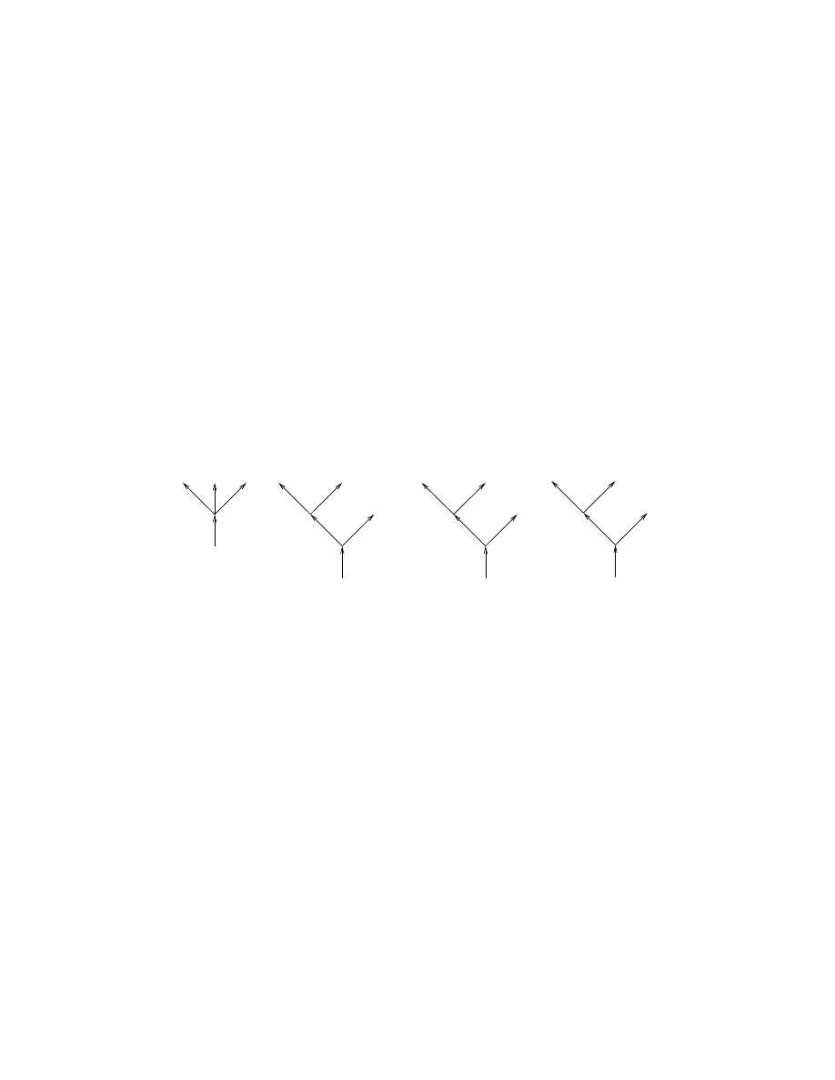
46
5. MOMENTS AND ABSOLUTE CONTINUITY PROPERTIES OF SUPERDIFFUSIONS
We consider monomials like {{ϕ
3
ϕ
2
}ϕ
1
{ϕ
4
ϕ
5
}}. There exist one monomial {ϕ
1
ϕ
2
}
of degree 2 and four distinguishable monomials of degree 3:
(2.3)
{ϕ
1
ϕ
2
ϕ
3
}, {{ϕ
1
ϕ
2
}ϕ
3
}, {{ϕ
2
ϕ
3
}ϕ
1
}, {{ϕ
3
ϕ
1
}ϕ
2
}.
It follows from (2.1) and (2.2) that, for C = {i
1
, . . . , i
n
}, z(f
C
) is equal to the sum
of all monomials of degree n of ϕ
i
1
, . . . , ϕ
i
n
.
Formulae (1.6) and (1.8) imply
(2.4)
N
x
e
−h1,X
D
i
hf
1
, X
D
i . . . hf
n
, X
D
i = z(f
1
, . . . , f
n
)(x)
for all x ∈ D
and
(2.5) P
µ
e
−h1,X
D
i
hf
1
, X
D
i . . . hf
n
, X
D
i = e
−hV
D
(1),µi
X
P
(C)
hz(f
C
1
), µi . . . hz(f
C
r
), µi
where C = {1, . . . , n}.
2.2.
A diagram D ∈ D
n
is a rooted tree with the leaves marked by 1, 2, . . ., n.
To every monomial of degree n there corresponds D ∈ D
n
. Here are the diagrams
corresponding to the monomials (2.3):
2
3
2
1
3
1
2
3
1
1
2
3
Figure 1
Every diagram consists of a set V of vertices (or sites) and a set A of arrows.
We write a : v → v
0
if v is the beginning and v
0
is the end of an arrow a. We
denote by a
+
(v) the number of arrows which end at v and by a
−
(v) the number
of arrows which begin at v. Note that a
+
(v) = 0, a
−
(v) = 1 for the root and
a
+
(v) = 1, a
−
(v) = 0 for leaves.
We label each site v of D ∈ D
n
by a variable y
v
. We take y
v
= x for the root
v and y
v
= z
i
for the leaf i. We also label every arrow a : v → v
0
by a kernel
r
a
(y
v
, dy
v
0
). Here r
a
is one of two kernels corresponding to the operators G
`
D
and
K
`
D
by the formulae
G
`
D
f (x) =
Z
D
g
`
D
(x, dy)f (y)
and
K
`
D
f (x) =
Z
∂D
k
`
D
(x, dy)f (y).
More precisely, if a = v → v
0
, then r
a
= g
`
D
(y
v
, dy
v
0
) if v, v
0
are not leaves and
r
a
= k
`
D
(y
v
, dz
i
) if v
0
is a leaf i. We associate with D ∈ D
n
a function
(2.6)
z
D
(f
1
, . . . , f
n
) =
Z Y
a∈A
r
a
(y
v
, dy
v
0
)
Y
v∈V
q
a
−
(v)
(y
v
)
n
Y
1
k
`
D
(y
v
i
, dz
i
)f
i
(z
i
)

3. ABSOLUTE CONTINUITY RESULTS
47
where v
i
is the beginning of the arrow with the end at a leaf i.
3
Examples. For the first diagram on Figure 1,
z
D
(f
1
, f
2
, f
3
) =
Z
g
`
D
(x, dy)q
3
(y)k
`
D
(y, dz
1
)f
1
(z
1
)k
`
D
(y, dz
2
)f
2
(z
2
)k
`
D
(y, dz
3
)f
3
(z
3
).
For the second diagram,
z
D
(f
1
, f
2
, f
3
) =
Z
g
`
D
(x, dy
1
)q
2
(y
1
)k
`
D
(y
1
, dz
3
)f
3
(z
3
)
g
`
D
(y
1
, dy
2
)q
2
(y
2
)k
`
D
(y
2
, dz
1
)f
1
(z
1
)k
`
D
(y
2
, dz
2
)f
2
(z
2
).
We note that
(2.7)
z(f
1
, . . . , f
n
) =
X
D∈D
n
z
D
(f
1
, . . . , f
n
).
3. Absolute continuity results
3.1.
In this section we prove:
Theorem 3.1. Let D be a bounded domain of class C
2,λ
and let γ be the surface
area on ∂D. For every Borel subset B of (∂D)
n
,
(3.1)
N
x
e
−h1,X
D
i
Z
B
X
D
(dy
1
) . . . X
D
(dy
n
)
=
Z
B
ρ
x
(y
1
, . . . , y
n
)γ(dy
1
) . . . γ(dy
n
)
with a strictly positive ρ
x
.
For every µ ∈ M
c
(D),
(3.2)
P
µ
e
−h1,X
D
i
Z
B
X
D
(dy
1
) . . . X
D
(dy
n
)
= e
−hV
D
(1),µi
Z
B
ρ
µ
(y
1
, . . . , y
n
)γ(dy
1
) . . . γ(dy
n
)
with a strictly positive ρ
µ
.
Theorem 3.1 implies that the class of null sets for each of measures (0.2) and
(0.3) (we call them the moment measures) coincides with the class of null sets for
the measure γ
n
. In other words, all these measures are equivalent.
Theorem 3.2. Suppose A ∈ F
⊃D
. Then either P
µ
(A) = 0 for all µ ∈ M
c
(D)
or P
µ
(A) > 0 for all µ ∈ M
c
(D).
If A ∈ F
∂
, then either P
µ
(A) = 0 for all µ ∈ M
c
(E) or P
µ
(A) > 0 for all
µ ∈ M
c
(E).
3
We put q
0
= 1 to serve leaves v for which a
−
(v) = 0.

48
5. MOMENTS AND ABSOLUTE CONTINUITY PROPERTIES OF SUPERDIFFUSIONS
3.2. Proof of Theorem 3.1. It is sufficient to prove that formulae (3.1) and
(3.2) hold for B = B
1
× · · · × B
n
where B
1
, . . . , B
n
are Borel subsets of ∂D. If we
demonstrate that
(3.3)
z
D
(f
1
, . . . , f
n
) =
Z
ρ
D
(y
1
, . . . , y
n
)f
1
(y
1
) . . . f
n
(y
n
)γ(dy
1
) . . . γ(dy
n
)
with ρ
D
> 0 for f
1
= 1
B
1
, . . . , f
n
= 1
B
n
, then (3.1) and (3.2) will follow from (2.4),
(2.5) and (2.7). For a domain D of class C
2,λ
, k
`
D
(x, dy) = k
`
D
(x, y)γ(dy) where
k
`
D
(x, y) is the Poisson kernel for Lu − `u. Since k
`
D
(x, y) > 0, formula (2.6) implies
(3.3).
To prove Theorem 3.2 we need some preparations.
3.3. Poisson random measure.
Theorem 3.3. Suppose that R is a finite measure on a measurable space (S, B).
Then there exists a random measure (Y, Q) on S with the properties:
(a) Y (B
1
), . . . , Y (B
n
) are independent for disjoint B
1
, . . . , B
n
;
(b) Y (B) is a Poisson random variable with the mean R(B), i.e.,
Q{Y (B) = n} =
1
n!
R(B)
n
e
−R(B)
for n = 0, 1, 2, . . . .
For every function F ∈ B ,
(3.4)
Qe
−hF,Y i
= exp[−
Z
S
(1 − e
−F (z)
)R(dz)].
Proof. Consider independent identically distributed random elements Z
1
, . . . , Z
n
, . . .
of S with the probability distribution ¯
R(B) = R(B)/R(S). Let N be the Pois-
son random variable with mean value R(S) independent of Z
1
, . . . , Z
n
, . . . . Put
Y (B) = 1
B
(Z
1
) + · · · + 1
B
(Z
N
). Note that Y = δ
Z
1
+ · · · + δ
Z
N
where δ
z
is the unit
measure concentrated at z. Therefore hF, Y i =
P
N
1
F (Z
i
) and (3.4) follows from
the relation
Qe
−hF,Y i
=
∞
X
m=0
1
m!
R(S)
m
e
−R(S)
m
Y
1
Qe
−F (Z
i
)
.
By taking F = λ1
B
we get
Qe
−λY (B)
= exp[−(1 − e
−λ
)R(B)]
which implies the property (b). If B
1
, . . . , B
n
are disjoint, then, by applying (3.4)
to F =
P
n
1
λ
i
1
B
i
, we get
Qe
−
P
λ
i
Y (B
i
)
= e
−
P
(1−e
−λi
)R(B
i
)
=
Y
Qe
−λ
i
Y (B
i
)
which implies (a).
We conclude from (3.4) that (Y, Q) is an infinitely divisible random measure.
It is called the Poisson random measure with intensity R. This is an integer-valued
measure concentrated on a finite random set.

3. ABSOLUTE CONTINUITY RESULTS
49
3.4. Poisson representation of infinitely divisible measures.
Theorem 3.4. Let (X, P ) be an infinitely divisible measure on a measurable
Luzin space E with the canonical measure R. Consider the Poisson random measure
(Y, Q) on S = M(E) with intensity R and put ˜
X (B) =
R
M
ν(B)Y (dν). The
random measure ( ˜
X , Q) has the same probability distribution as (X, P ) and, for
every F ∈ B
M
, we have
(3.5)
P F (X) = QhF, Y i =
∞
X
0
1
n!
e
−R(M)
Z
R(dν
1
) . . . R(dν
n
)F (ν
1
+ · · · + ν
n
).
Proof. Note that hf, ˜
Xi = hF, Y i where F (ν) = hf, νi. By (3.4), we get
Qe
−h
f, ˜
X i
= Qe
−h
F,Y i
= exp
−
Z
M
(1 − e
−h
f,νi
)R(dν)
.
This implies the first part of the theorem. The second part follows from the ex-
pression Y (B) = 1
B
(Z
1
) + · · · + 1
B
(Z
N
) for Y introduced in the proof of Theorem
3.3.
3.5. Proof of Theorem 3.2. 1
◦
. By applying Theorem 3.4 to the random
measure (P
µ
, X
D
) and a function e
−h1,νi
F (ν) we get
(3.6)
P
µ
e
−h1,X
D
i
F (X
D
)
=
∞
X
0
1
n!
Z
D
(µ)
Z
R
∗
µ
(dν
1
) . . . R
∗
µ
(dν
n
)F (ν
1
+ · · · + ν
n
)
where
(3.7)
Z
D
(µ) = e
−R
µ
[M(D)]
,
and R
∗
µ
(dν) = e
−h1,νi
R
µ
(dν).
2
◦
. Let F be a positive measurable function on M(∂D) and let
f
n
(x
1
, . . . , x
n
) =
Z
F (ν
1
+ · · · + ν
n
)R
∗
x
1
(dν
1
) . . . R
∗
x
n
(dν
n
).
We prove that, if ˜
D b D and µ ∈ M
c
( ˜
D), then F (X
D
) = 0 P
µ
-a.s. if and only if
(3.8)
Z
f
n
(x
1
, . . . , x
n
)γ
˜
D
(dx
1
) . . . γ
˜
D
(dx
n
) = 0
for all n.
Indeed, by the Markov property of X,
(3.9)
P
µ
e
−h1,X
D
i
F (X
D
) = P
µ
P
X
˜
D
e
−h1,X
D
i
F (X
D
).
By (3.6) and (3.9),
(3.10)
P
µ
e
−h1,X
D
i
F (X
D
) =
∞
X
n=0
1
n!
P
µ
Z
D
(X
˜
D
)
Z
X
˜
D
(dx
1
) . . . X
˜
D
(dx
n
)f
n
(x
1
, . . . , x
n
).
Since Z
D
(X
˜
D
) > 0, the condition F (X
D
) = 0 P
µ
-a.s. is equivalent to the condition:
for every n,
(3.11)
Z
X
˜
D
(dx
1
) . . . X
˜
D
(dx
n
)f
n
(x
1
, . . . , x
n
) = 0
P
µ
-a.s.
It follows from Theorem 3.1, that the condition (3.11) is equivalent to the condition
(3.8).

50
5. MOMENTS AND ABSOLUTE CONTINUITY PROPERTIES OF SUPERDIFFUSIONS
3
◦
. Suppose µ
1
and µ
2
belong to M
c
(D). There exists ˜
D b D which contains
supports of µ
1
and µ
2
. By 2
◦
, F (X
D
) = 0 P
µ
1
-a.s. if and only if F (X
D
) = 0
P
µ
2
-a.s. If A ∈ F
⊃D
, then by the Markov property of X,
P
µ
i
(A) = P
µ
i
F (X
D
)
where F (ν) = P
ν
(A). This implies the first statement of Theorem 3.2.
If µ
1
, µ
2
∈ M
c
(E), then µ
1
, µ
2
∈ M
c
(D) for a domain of class C
2,λ
such that
D b E. If A ∈ F
∂
, then A ∈ F
⊃D
and the second part of Theorem 3.2 follows from
the first one.
4. Notes
4.1.
The results of the first two sections are applicable to all (ξ, ψ)-superprocesses
described in Section 3.2.2, and the proofs do not need any modification. The abso-
lute continuity results can be extended to (ξ, ψ)-superprocesses under an additional
assumption that the Martin boundary theory is applicable to ξ.
4
The boundary
∂E and the Poisson kernel are to be replaced by the Martin boundary and the
Martin kernel. The role of the surface area is played by the measure corresponding
to the harmonic function h = 1.
4.2.
A diagram description of moments of higher order was given, first, in
[Dyn88]. There only ψ(u) = u
2
was considered. In [Dyn91b] the moments of order
n were evaluated under the assumption that ψ of the form 3.(2.8) has a bounded
continuous derivative
d
n
ψ
du
n
. [See also [Dyn04a].] Brief description of these results
is given on pages 201–203 of [D].
5
The main recent progress is the elimination of
the assumption about differentiability of ψ which allows to cover the case ψ(u) =
u
α
, 1 < α < 2.
4.3.
The first absolute continuity results for superprocesses were obtained
in [EP91]. Let (X
t
, P
µ
) be a (ξ, ψ)-superprocess with ψ(u) = u
2
/2. To every
µ ∈ M(E) there correspond measures p
µ
t
on E and measures Q
µ
t
on M(E) defined
by the formulae
p
µ
t
(B) =
Z
µ(dx)Π
x
{ξ
t
∈ B},
Q
µ
t
(C) = P
µ
{X
t
∈ C}.
Let h > 0. Evans and Perkins proved that Q
µ
1
t
is absolutely continuous with respect
to Q
µ
2
t+h
for all t > 0 if and only if p
µ
1
t
is absolutely continuous with respect to p
µ
2
t+h
for all t > 0.
Independently, Mselati established an absolute continuity property for the ex-
cursion measures N
x
of the Brownian snake: if C belongs to the σ-algebra gener-
ated by the stochastic values of all subsolutions and supersolutions of the equation
∆u = u
2
, then, for every x
1
, x
2
∈ E, N
x
1
(C) = 0 if N
x
2
(C) = 0. (See Proposition
2.3.5 in [Mse02a] or Proposition 2.18 in [Mse04].)
4
The key condition – the existence of a Green’s function – is satisfied for L-diffusions in a
wide class of the so-called Greenian domains. The Martin boundary theory for such domains can
be found in Chapter 7 of [D].
5
Figure 1.2 is borrowed from page 202 in [D]. We also corrected a few misprints in formulae
which could confuse a reader.[For instance the value of q
m
on pages 201–203 must be multiplied
by (−1)
m
.]

4. NOTES
51
A proof of Theorem 3.2 is given in [Dyn04c]. The case of infinitely differentiable
ψ was considered earlier in [Dyn04a], Theorem 6.2.


CHAPTER 6
Poisson capacities
A key part of the proof that all solutions of the equation ∆u = u
α
are σ-
moderate is establishing bounds for w
Γ
and u
Γ
in terms of a capacity of Γ. In the
case α = 2, Mselati found such bounds by using Cap
∂
introduced by Le Gall. This
kind of capacity is not applicable for α 6= 2. We replace it by a family of Poisson
capacities. In this chapter we establish relations between these capacities which
will be used in Chapters 8 and 9.
The Poisson capacities are a special case of (k, m)-capacities described in Sec-
tion 1.
1. Capacities associated with a pair (k, m)
1.1. Three definitions of (k, m)-capacities. Fix α > 1.
Suppose that
k(x, y) is a positive lower semicontinuous function on the product E × ˜
E of two
separable locally compact metric spaces and m is a Radon measure on E. A (k, m)-
capacity is a Choquet capacity on ˜
E. We give three equivalent definitions of this
capacity.
Put
(1.1)
(Kν)(x) =
Z
˜
E
k(x, y)ν(dy),
E (ν) =
Z
E
(Kν)
α
dm
for ν ∈ M( ˜
E)
and
(1.2)
ˆ
K(f )(y) =
Z
E
m(dx)f (x)k(x, y)
for f ∈ B(E).
Define Cap(Γ) for subsets Γ of ˜
E by one of the following three formulae:
(1.3)
Cap(Γ) = sup{E (ν)
−1
: ν ∈ P(Γ)},
(1.4)
Cap(Γ) = [sup{ν(Γ) : ν ∈ M(Γ), E (ν) ≤ 1}]
α
,
(1.5)
Cap(Γ) = [inf{
Z
E
f
α
0
dm : f ∈ B(E), ˆ
Kf ≥ 1
on Γ}]
α−1
where α
0
= α/(α − 1). We refer to [AH96], Chapter 2 for the proof that the Cap(Γ)
defined by (1.4) or by (1.5) satisfies the conditions 2.4.A, 2.4.B and 2.4.C and
therefore all Borel subsets are capacitable.
1
[The equivalence of (1.4) and (1.5) is
proved also in [D], Theorem 13.5.1.]
1
In [AH96] a wider class of kernels is considered. The result is stated for the case E = R
d
but no specific property of R
d
is used in the proofs.
53

54
6. POISSON CAPACITIES
To prove the equivalence of (1.3) and (1.4), we note that ν ∈ M(Γ) is equal to
tµ where t = ν(Γ) and µ = ν/t ∈ P(Γ) and
sup
ν∈M(Γ)
{ν(Γ) : E (ν) ≤ 1} =
sup
µ∈P(Γ)
sup
t≥0
{t : t
α
E (µ) ≤ 1} =
sup
µ∈P(Γ)
E (µ)
−1/α
.
2. Poisson capacities
In this chapter we deal with a special type of (k, m)-capacities associated with
the Poisson kernel k = k
E
for an operator L. The function k
E
(x, y) is continuous
on E × ˜
E where E is a C
2,λ
-domain in R
d
and ˜
E = ∂E. We use notation Cap for
the Poisson capacity corresponding to
(2.1)
m(dx) = ρ(x)dx
with ρ(x) = d(x, ∂E)
and we denote by Cap
x
the Poisson capacity corresponding to
(2.2)
m(dy) = g
E
(x, y)dy
where g
E
is the Green function in E for L. [In the case of Cap
x
, E (ν) has to be
replaced by
E
x
(ν) =
Z
E
g
E
(x, y)h
ν
(y)
α
dy = [G
E
(Kν)
α
](x)
in formulae (1.3)–(1.4).]
2.1. Results. An upper bound of Cap(Γ) is given by:
Theorem 2.1. For all Γ ∈ B(∂E),
(2.3)
Cap(Γ) ≤ C diam(Γ)
γ
+
where
(2.4)
γ = dα − d − α − 1
and γ
+
= γ ∨ 0.
The second theorem establishes a lower bound for Cap
x
in terms of Cap.
The values α < (d + 1)/(d − 1) are called subcritical and the values α ≥
(d + 1)/(d − 1) are called supercritical.
Theorem 2.2. Suppose that L is an operator of divergence form 1.(4.2) and
d ≥ 3. Put
(2.5)
ϕ(x, Γ) = ρ(x)d(x, Γ)
−d
.
If α is subcritical, then there exists a constant C > 0 such that
(2.6)
Cap
x
(Γ) ≥ Cϕ(x, Γ)
−1
Cap(Γ).
for all Γ and x.
If α is supercritical, then, for every κ > 0 there exists a constant C
κ
> 0 such
that
(2.7)
Cap
x
(Γ) ≥ C
κ
ϕ(x, Γ)
−1
Cap(Γ)
for all Γ and x subject to the condition
(2.8)
d(x, Γ) ≥ κ diam(Γ).

3. UPPER BOUND FOR Cap(Γ)
55
3. Upper bound for Cap(Γ)
To prove Theorem 2.1 we use the straightening of the boundary described in
Section 4.2 of the Introduction. As the first step, we consider a capacity on the
boundary E
0
= {x = (x
1
, . . . , x
d
) : x
d
= 0} of a half-space E
+
= {x = (x
1
, . . . , x
d
) :
x
d
> 0} = R
d−1
× (0, ∞).
3.1. Capacity g
Cap. Put
r(x) = d(x, E
0
) = x
d
,
E = {x = (x
1
, . . . , x
d
) : 0 < x
d
< 1},
˜
k(x, y) = r(x)|x − y|
−d
, x ∈ E, y ∈ E
0
(3.1)
and consider a measure
(3.2)
˜
m(dx) = r(x)dx
on E. Denote by g
Cap the (˜
k, ˜
m)-capacity on E
0
.
Note that
˜
k(x/t, y/t) = t
d−1
˜
k(x, y)
for all t > 0.
To every ν ∈ P(E
0
) there corresponds a measure ν
t
∈ P(E
0
) defined by the formula
ν
t
(B) = ν(tB). We have
Z
E
0
f (y)ν
t
(dy) =
Z
E
0
f (y/t)ν(dy)
for every function f ∈ B(E
0
). Put ˜
h
ν
= ˜
K ν. Note that
(3.3)
˜
h
ν
t
(x/t) =
Z
E
0
˜
k(x/t, y)ν
t
(dy) =
Z
E
0
˜
k(x/t, y/t)ν(dy) = t
d−1
˜
h
ν
(x).
Change of variables x = t˜
x and (3.3) yield
˜
E(ν
t
) = t
γ
˜
E (ν, tE)
where
˜
E (ν) =
Z
E
˜
h
α
ν
d ˜
m,
˜
E(ν, B) =
Z
B
˜
h
α
ν
d ˜
m
for B ∈ B(E
+
) and γ defined by (2.4).
If t ≥ 1, then tE ⊃ E and we have
(3.4)
˜
E (ν
t
) ≥ t
γ
˜
E (ν).
Lemma 3.1. If diam(Γ) ≤ 1, then
(3.5)
g
Cap(Γ) ≤ C
d
(diam(Γ))
γ
.
The constant C
d
depends only on the dimension d. (It is equal to g
Cap(U ) where
U = {x ∈ E
0
: |x| ≤ 1}.
Proof. Since g
Cap is translation invariant, we can assume that 0 ∈ Γ. Let
t = diam(Γ)
−1
. Since tΓ ⊂ U , we have
(3.6)
g
Cap(tΓ) ≤ g
Cap(U ).
Since ν → ν
t
is a 1-1 mapping from P(tΓ) onto P(Γ), we get
g
Cap(Γ) =
sup
ν
t
∈P(Γ)
˜
E (ν
t
)
−1
=
sup
ν∈P(tΓ)
˜
E (ν
t
)
−1
.

56
6. POISSON CAPACITIES
Therefore, by (3.4) and (1.3),
g
Cap(Γ) ≤ t
−
γ
g
Cap(tΓ)
and (3.6) implies (3.5).
3.2. Three lemmas.
Lemma 3.2. Suppose that E
1
, E
2
, E
3
are bounded domains, E
1
and E
2
are
smooth and ¯
E
2
⊂ E
3
. Then there exists a smooth domain D such that
(3.7)
E
1
∩ E
2
⊂ D ⊂ E
1
∩ E
3
.
Proof. The domain D
0
= E
1
∩ E
2
is smooth outside L = ∂E
1
∩ ∂E
2
. We
get D by a finite number of small deformations of D
0
near L. Let q ∈ L and let
U be the ε-neighborhood of q. Consider coordinates (y
1
, y
2
, . . . , y
d
) in U and put
y = (y
1
, . . . , y
d−1
), r = y
d
. If ε is sufficiently small, then the coordinate system can
be chosen in which the intersections of E
i
with U are described by the conditions r <
f
i
(y) where f
1
, f
2
, f
3
are smooth functions. There exists an infinitely differentiable
function a(r) such that r ∧ 0 ≤ a(r) ≤ r ∧ ε and a(r) = 0 for r > ε/2. Put
g = f
2
+ a(f
1
− f
2
) and replace the part of D
0
in U by {(y, r) : r < g(y)} without
changing the part outside U . Since g ≥ f
1
∧ f
2
, we get a domain D
1
which contains
D
0
. Since g ≤ f
1
∧ (f
2
+ ε), D
1
is contained in E
3
if ε is sufficiently small. Finally,
the portion of ∂D
1
in U is smooth. After a finite number of deformations of this
kind we get a smooth domain which satisfies the condition (3.7).
Lemma 3.3. Suppose E ⊂ E, 0 ∈ Γ ⊂ ∂E ∩ E
0
and put A = E \ E, B
λ
= {x ∈
E : |x| < λ}. If d(Γ, A) > 2λ, then B
λ
⊂ E and r(x) = ρ(x) for x ∈ B
λ
.
Proof. If x ∈ B
λ
, then r(x) ≤ |x| < λ. If x ∈ B
λ
and y ∈ A, then |x − y| ≥
|y| − |x| > λ because |y| ≥ d(y, Γ) ≥ d(A, Γ) > 2λ. Hence d(x, A) ≥ λ which implies
that B
λ
⊂ E.
For x ∈ E, ρ(x) = d(x, E
c
), r(x) = d(x, E
c
+
) and therefore ρ(x) ≤ r(x). Put
A
1
= ∂E ∩ A, A
2
= ∂E ∩ E
0
. For every x ∈ E, d(x, A
1
) = d(x, A), d(x, A
2
) ≥ r(x)
and ρ(x) = d(x, A
1
) ∧ d(x, A
2
) ≥ d(x, A) ∧ r(x). If x ∈ B
λ
, then r(x) < λ ≤ d(x, A)
and therefore ρ(x) ≥ r(x). Hence ρ(x) = r(x).
Lemma 3.4. There exists a constant C
λ
> 0 such that
(3.8)
˜
E(ν, B
λ
) ≥ C
λ
˜
E (ν)
for all ν ∈ P(Γ) and for all Γ 3 0 such that diam(Γ) < λ/2.
Proof. If x ∈ F
λ
= E \ B
λ
and y ∈ Γ, then |y| ≤ diam(Γ) < λ/2 ≤ |x|/2 and
therefore |x − y| > |x| − |y| ≥ |x|/2. This implies
˜
h
ν
(x) ≤ r(x)2
d
|x|
−d
and
(3.9)
˜
E (ν, F
λ
) ≤ 2
dα
Z
F
λ
r(x)
α+1
|x|
−dα
dx = C
0
λ
< ∞.
On the other hand, if x ∈ B
λ
, y ∈ Γ, then |x − y| ≤ |x| + |y| ≤ 3λ/2. Therefore
˜
h
ν
(x) ≥ (3λ/2)
−d
r(x) and
(3.10)
˜
E(ν, B
λ
) ≥ (3λ/2)
−dα
Z
B
λ
r(x)
α+1
dx = C
00
λ
> 0.

3. UPPER BOUND FOR Cap(Γ)
57
It follows from (3.9) and (3.10) that
C
0
λ
˜
E (ν, B
λ
) ≥ C
0
λ
C
00
λ
≥ C
00
λ
˜
E(ν, F
λ
) = C
00
λ
[ ˜
E(ν) − ˜
E (ν, B
λ
)]
and (3.8) holds with C
λ
= C
00
λ
/(C
0
λ
+ C
00
λ
).
3.3. Straightening of the boundary.
Proposition 3.1. Suppose that E is a bounded smooth domain. Then there
exist strictly positive constants ε, a, b (depending only on E) such that, for every
x ∈ ∂E:
(a) The boundary can be straightened in B(x, ε).
(b) The corresponding diffeomorphism ψ
x
satisfies the conditions
(3.11)
a
−
1
|y
1
− y
2
| ≤ |ψ
x
(y
1
) − ψ
x
(y
2
)| ≤ a|y
1
− y
2
|
for all y
1
, y
2
∈ B(x, ε);
(3.12)
a
−1
diam(A) ≤ diam(ψ
x
(A)) ≤ a diam(A)
for all A ⊂ B(x, ε);
(3.13)
a
−1
d(A
1
, A
2
) ≤ d(ψ
x
(A
1
), ψ
x
(A
2
)) ≤ a d(A
1
, A
2
)
for all A
1
, A
2
⊂ B(x, ε).
(3.14)
b
−1
≤ J
x
(y) ≤ b
for all y ∈ B(x, ε)
where J
x
(y) is the Jacobian of ψ
x
at y.
Diffeomorphisms ψ
x
can be chosen to satisfy additional conditions
(3.15)
ψ
x
(x) = 0
and ψ
x
(B(x, ε)) ⊂ E.
Proof. The boundary ∂E can be covered by a finite number of balls B
i
=
B(x
i
, ε
i
) in which straightening diffeomorphisms are defined. The function q(x) =
max
i
d(x, B
c
i
) is continuous and strictly positive on ∂E. Therefore ε =
1
2
min
x
q(x) >
0. For every x ∈ ∂E there exists B
i
which contains the closure of B(x, ε). We put
ψ
x
(y) = ψ
x
i
(y)
for y ∈ B(x, ε).
This is a diffeomorphism straightening ∂E in B(x, ε).
For every x, B(x, ε) is contained in one of closed balls ˜
B
i
= {y : d(y, B
c
i
) ≥ ε}.
Since ψ
x
i
belongs to the class C
2,λ
(B
i
), there exist constants a
i
> 0 such that
a
−1
i
|y
1
− y
2
| ≤ |ψ
x
i
(y
1
) − ψ
x
i
(y
2
)| ≤ a
i
|y
1
− y
2
|
for all y
1
, y
2
∈ ˜
B
i
.
The condition (3.11) holds for a = max a
i
. The conditions (3.12) and (3.13) fol-
low from (3.11). The Jacobian J
x
i
does not vanish at any point y ∈ B
i
and we
can assume that it is strictly positive. The condition (3.14) holds because J
x
i
is
continuous on the closure of B(x, ε).
By replacing ψ
x
(y) with c[ψ
x
(y) − ψ
x
(x)] with a suitable constant c, we get
diffeomorphisms subject to (3.15) in addition to (3.11)-(3.14).
3.4. Proof of Theorem 2.1. 1
◦
. If γ < 0, then (2.3) holds because Cap(Γ) ≤
Cap(∂E) = C. To prove (2.3) for γ ≥ 0, it is sufficient to prove that, for some
β > 0, there is a constant C
1
such that
Cap(Γ) ≤ C
1
diam(Γ)
γ
if diam(Γ) ≤ β.
Indeed,
Cap(Γ) ≤ C
2
diam(Γ)
γ
if diam(Γ) ≥ β
with C
2
= Cap(∂E)β
−γ
.

58
6. POISSON CAPACITIES
2
◦
. Let ε, a be the constants defined in Proposition 3.1 and let β = ε/(2 + 8a
2
) ∧
1. Suppose that diam(Γ) ≤ β and let x ∈ Γ. Consider a straightening ψ
x
of ∂E
in B(x, ε) which satisfies conditions (3.15). Put B = B(x, ε), ˜
B = B(x, ε/2). By
Lemma 3.2, there exists a smooth domain D such that ˜
B ∩ E ⊂ D ⊂ B ∩ E. Note
that ˜
B ∩ ∂E ⊂ ∂D ∩ ∂E ⊂ B ∩ ∂E. If A
1
= ∂D ∩ B ∩ E, then d(x, A
1
) ≥ ε/2
and d(Γ, A
1
) ≥ ε/2 − diam(Γ) ≥ ε/2 − β. Denote by D
0
, Γ
0
, A
0
1
the images of
D, Γ, A
1
under ψ
x
and let A
0
= E \ D
0
. By (3.12), diam(Γ
0
) ≤ λ
1
= aβ and
d(Γ
0
, A
0
) ≥ λ
2
= (ε/2 − β)/a. Our choice of β implies that λ
1
< λ
2
/4. Put
λ = λ
1
+ λ
2
/4. Note that λ
2
> 2λ and λ
1
< λ/2. Since d(Γ
0
, A
0
) = d(Γ, A
0
1
),
Lemmas 3.3 and 3.4 are applicable to D
0
, Γ
0
, A
0
and λ (which depends only on E).
3
◦
. By 2.(1.10) and (3.13), for every y ∈ D, z ∈ Γ,
(3.16)
k
E
(y, z) ≥ Cd(y, ∂E)|y − z|
−
d
≥ Cd(y, ∂D)|y − z|
−d
≥ Cd(y
0
, ∂D
0
)|y
0
− z
0
|
−d
where y
0
= ψ
x
(y), z
0
= ψ
x
(z). If ν
0
is the image of ν ∈ P(Γ) under ψ
x
, then
Z
Γ
f [ψ
x
(z)]ν(dz) =
Z
Γ
0
f (z
0
)ν
0
(dz
0
)
for every positive measurable function f . In particular,
(3.17)
Z
Γ
|y
0
− ψ
x
(z)|
−d
ν(dz) =
Z
Γ
0
|y
0
− z
0
|
−d
ν
0
(dz
0
).
By (3.16) and (3.17),
Z
Γ
k
E
(y, z)ν(dz) ≥ Cd(y
0
, ∂D
0
)
Z
Γ
0
|y
0
− z
0
|
−d
ν
0
(dz
0
).
If y
0
∈ B
λ
, then, by Lemma 3.3, d(y
0
, ∂D
0
) = r(y
0
) and we have
(3.18)
h
ν
(y) =
Z
Γ
k
E
(y, z)ν(dz) ≥ C
Z
Γ
0
r(y
0
)|y
0
− z
0
|
−d
ν
0
(dz
0
) = C˜
h
ν
0
[ψ
x
(y)].
If y ∈ D, then, by (3.13), d(y, ∂E) ≥ d(y, ∂D) ≥ Cd(y
0
, ∂D
0
) and therefore
(1.1), (2.1) and (3.18) imply
(3.19)
E (ν) =
Z
E
d(y, ∂E)h
ν
(y)
α
dy ≥
Z
D
d(y, ∂D)h
ν
(y)
α
dy
≥ C
Z
D
d(ψ
x
(y), ∂D
0
)˜
h
ν
0
[ψ
x
(y)]
α
dy.
Note that
Z
D
0
f (y
0
)dy
0
=
Z
D
f [ψ
x
(y)]J
x
(y)dy
and, if f ≥ 0, then, by (3.14),
Z
D
0
f (y
0
)dy
0
≤ b
Z
D
f [ψ
x
(y)]dy.
By taking f (y
0
) = d(y
0
, ∂D
0
)˜
h
ν
0
(y
0
)
α
, we get from (3.19)
E (ν) ≥ C
Z
D
0
d(y
0
, ∂D
0
)˜
h
ν
0
(y
0
)
α
dy
0
.

4. LOWER BOUND FOR Cap
x
59
By Lemma 3.3, D
0
⊃ B
λ
and d(y
0
, ∂D
0
) = r(y
0
) on B
λ
. Hence
E (ν) ≥ C
Z
B
λ
r(y
0
)˜
h
ν
0
(y
0
)
α
dy
0
= C ˜
E(ν
0
, B
λ
).
By Lemma 3.4, this implies E (ν) ≥ C ˜
E(ν
0
) and, by (1.3), Cap(Γ) ≤ C d
Cap(Γ
0
). The
bound Cap(Γ) ≤ C diam(Γ)
γ
follows from Lemma 3.1, (3.12) and 1
◦
.
4. Lower bound for Cap
x
4.1.
Put
δ(x) = d(x, Γ),
E
1
= {x ∈ E : δ(x) < 3ρ(x)/2},
E
2
= E \ E
1
;
E
x
(ν, B) =
Z
B
g(x, y)h
ν
(y)
α
dy
for B ⊂ E
(4.1)
and let
(4.2)
U
x
= {y ∈ E : |x − y| < δ(x)/2},
V
x
= {y ∈ E : |x − y| ≥ δ(x)/2}.
First, we deduce Theorem 2.2 from the following three lemmas. Then we prove
these lemmas.
Lemma 4.1. For all Γ, all ν ∈ P(Γ) and all x ∈ E,
(4.3)
E
x
(ν, V
x
) ≤ Cϕ(x, Γ)E (ν).
Lemma 4.2. For all Γ, all ν ∈ P(Γ) and all x ∈ E
1
,
(4.4)
E
x
(ν, U
x
) ≤ Cϕ(x, Γ)E (ν).
Lemma 4.3. For all Γ, all ν ∈ P(Γ) and all x ∈ E
2
,
(4.5)
E
x
(ν, U
x
) ≤ Cϕ(x, Γ)θ(x)
−γ
+
E (ν)
where
θ(x) = d(x, Γ)/ diam(Γ).
4.2. Proof of Theorem 2.2. By Lemmas 4.2 and 4.3, for every x ∈ E
E
x
(ν, U
x
) ≤ Cϕ(x, Γ)E (ν)(1 ∨ θ(x)
−γ
+
)
and therefore, under the condition (2.8),
E
x
(ν, U
x
) ≤ Cϕ(x, Γ)E (ν)(1 ∨ κ
−γ
+
).
This bound and Lemma 4.1 imply that
E
x
(ν) = E
x
(ν, U
x
) + E
x
(ν, V
x
) ≤ Cϕ(x, Γ)E (ν)[2 ∨ (1 + κ
−γ
+
)]
and, by (1.3),
(4.6)
Cap
x
(Γ) ≥ C
κ
ϕ(x, Γ)
−1
Cap(Γ)
where C
κ
= C
−1
[2 ∨ (1 + κ
−γ
+
)]
−1
. If α is subcritical, then γ < 0, C
κ
does not
depend on κ and (4.6) implies (2.6). If α is supercritical, then γ ≥ 0 and (2.7)
holds under the condition (2.8).
4.3. Proof of Lemma 4.1. By 2.(1.7),
E
x
(ν, V
x
) ≤ Cρ(x)
Z
V
x
ρ(y)|x − y|
−d
h
ν
(y)
α
dy.
Since |x − y| ≥ δ(x)/2 for y ∈ V
x
, this implies (4.3).

60
6. POISSON CAPACITIES
4.4. Proof of Lemma 4.2. The function h
ν
is harmonic in the ball {y :
|x − y|/ρ(x) ≤ r for 0 < r < 1. By the Harnack’s inequality,
(4.7)
1 − r
(1 + r)
d−1
h
ν
(x) ≤ h
ν
(y) ≤
1 + r
(1 − r)
d−1
h
ν
(x)
(see, e.g. [GT98], p.29, Problem 2.6). If x ∈ E
1
, y ∈ U
x
, then |x − y| < δ(x)/2 <
3ρ(x)/4 and (4.7) holds with r = 3/4. Therefore, for all x ∈ E
1
, y ∈ U
x
, C
0
d
h
ν
(x) ≤
h
ν
(y) ≤ C
00
d
h
ν
(x) where C
0
d
and C
00
d
depend only on d. This implies bounds
(4.8)
E
x
(ν, U
x
) ≤ C
00
d
h
ν
(x)
α
Z
U
x
g
E
(x, y)dy
and
(4.9)
E (ν) ≥
Z
U
x
ρ(y)h
ν
(y)
α
dy ≥ C
0
d
h
ν
(x)
α
Z
U
x
ρ(y)dy.
By 2.(1.6),
(4.10)
Z
U
x
g
E
(x, y)dy ≤ Cρ(x)
Z
U
x
|x − y|
1−d
dy = Cρ(x)
Z
δ(x)/2
0
dt ≤ Cδ(x)ρ(x).
For y ∈ U
x
, x ∈ E
1
,
ρ(y) ≥ ρ(x) − |x − y| ≥ ρ(x) − δ(x)/2 ≥ ρ(x)/4
and therefore
(4.11)
Z
U
x
ρ(y)dy ≥
1
4
ρ(x)
Z
U
x
dy = C
d
ρ(x)δ(x)
d
.
Since δρ ≤ 3ϕρδ
d
/2, bound (4.4) follows from (4.8)–(4.11).
4.5. Proof of Lemma 4.3. By Theorem 2.1,
E (ν)
−1
≤ Cap(Γ) ≤ C diam(Γ)
γ
+
.
Hence,
(4.12)
diam(Γ)
−γ
+
≤ CE (ν).
If x ∈ E
2
and y ∈ U
x
, then δ(y) ≥ δ(x) − |x − y| > δ(x)/2 and ρ(y) ≤
ρ(x) + |x − y| ≤ 2δ(x)/3 + δ(x)/2 = 7δ(x)/6. For all z ∈ Γ, y ∈ U
x
, |y − z| ≥
|z − x| − |y − x| ≥ δ(x)/2 and, by 2.(1.10),
k
E
(y, z) ≤ Cρ(y)|y − z|
−d
≤ Cδ(x)
1−d
.
Therefore h
ν
(y) ≤ Cδ(x)
1−d
and, by 2.(1.6),
(4.13)
E
x
(ν, U
x
) ≤ Cρ(x)δ(x)
(1−d)α
Z
U
x
|x − y|
1−d
dy ≤ Cϕ(x, Γ)δ(x)
−γ
.
If γ < 0, then δ(x)
−γ
≤ diam(E)
−γ
= C. If γ ≥ 0, then γ = γ
+
. Hence, the bound
(4.5) follows from (4.12) and (4.13).

5. NOTES
61
5. Notes
The capacity Cap defined by the formulae (1.3)–(1.5) with m defined by (2.1)
is related to a Poisson capacity CP
α
used in [D] by the equation
Cap(Γ) = CP
α
(Γ)
α
.
[The capacity CP
α
is a particular case of the Martin capacity also considered in
[D]. The Martin kernel is a continuous function on E × ˜
E where E is a domain on
R
d
(not necessarily smooth) and ˜
E is the Martin boundary of E for an L-diffusion.]
Let Cap
L
and Cap
x
be the Poisson capacities corresponding to an operator L. It
follows from 2.(1.10) that, for every L
1
and L
2
, the ratio Cap
L
1
/ Cap
L
2
is bounded
and therefore we can restrict ourselves by the Poisson capacities corresponding to
the Laplacian ∆.
The capacity CP
α
was introduced in [DK96b] as a tool for a study of removable
boundary singularities for solutions of the equation Lu = u
α
. It was proved that,
if E is a bounded smooth domain, then a closed subset Γ of ∂E is a removable
singularity if and only if CP
α
(Γ) = 0. First, this was conjectured in [Dyn94]. In
the case α = 2, the conjecture was proved by Le Gall [LG95] who used the capacity
Cap
∂
. Le Gall’s capacity Cap
∂
has the same class of null sets as CP
α
.
An analog of formula (2.7) with Cap replaced by Cap
∂
follows from formula
(3.34) in [Mse04] in the case L = ∆, α = 2, d ≥ 4 and κ = 4.
The results presented in Chapter 6 were published, first, in [DK03].


CHAPTER 7
Basic inequality
In this chapter we consider two smooth domains D ⊂ E, the set
(0.1)
D
∗
= {x ∈ ¯
D : d(x, E \ D) > 0}
and measures ν concentrated on ∂D ∩ ∂E. Our goal is to give a lower bound of
N
x
{R
E
⊂ D
∗
, Z
ν
6= 0} in terms of N
x
{R
E
⊂ D
∗
, Z
ν
} and E
x
(ν). This bound will
play an important role in proving the equation u
Γ
= w
Γ
in Chapter 8.
Preparations for proving the basic inequality include: (a) establishing relations
between R
E
and R
D
and between stochastic boundary values in E and D; (b)
expressing certain integrals with respect to the measures P
x
and N
x
through the
conditional diffusion Π
ν
x
.
1. Main result
Theorem 1.1. Suppose that D is a smooth open subset of a smooth domain E.
If ν is a finite measure concentrated on ∂D ∩ ∂E and if E
x
(ν) < ∞, then
(1.1)
N
x
{R
E
⊂ D
∗
, Z
ν
6= 0} ≥ C(α)[N
x
{R
E
⊂ D
∗
, Z
ν
}]
α/(α−1)
E
x
(ν)
−1/(α−1)
where C(α) = (α − 1)
−1
Γ(α − 1).
1
Remark. By 3.3.4.C, the condition E
x
(ν) < ∞ implies that ν belongs to N
E
1
and to N
D
1
.
2. Two propositions
2.1.
Proposition 2.1. Suppose x ∈ D, Λ is a Borel subset of ∂D and A = {R
D
∩
Λ = ∅}. We have P
x
A > 0 and for all Z
0
, Z
00
∈ Z
x
,
(2.1)
N
x
{A, (e
−Z
0
− e
−Z
00
)
2
}
= −2 log P
x
{e
−Z
0
−Z
00
| A} + log P
x
{e
−2Z
0
| A} + log P
x
{e
−2Z
00
| A}.
If Z
0
= Z
00
P
x
-a.s. on A and if P
x
{A, Z
0
< ∞} > 0, then Z
0
= Z
00
N
x
-a.s. on A.
Proof. First, P
x
A > 0 because, by 3.(3.9), P
x
A = e
−w
Λ
(x)
. Next,
(e
−Z
0
− e
−Z
00
)
2
= 2(1 − e
−Z
0
−Z
00
) − (1 − e
−2Z
0
) − (1 − e
−2Z
00
).
Therefore (2.1) follows from 4.(3.28). The second part of the proposition is an
obvious implication of (2.1).
1
Here Γ is Euler’s Gamma-function.
63

64
7. BASIC INEQUALITY
2.2.
Note that
(2.2)
D
∗
= {x ∈ ¯
D : d(x, Λ) > 0}
where Λ = ∂D ∩ E.
Proposition 2.2. Let D ⊂ E be two open sets. Then, for every x ∈ D, X
D
and X
E
coincide P
x
-a.s. and N
x
-a.s. on the set A = {R
D
⊂ D
∗
}.
Proof. By the Markov property 3.2.1.D, for every Borel set B,
(2.3)
P
x
{A, e
−X
E
(B)
} = P
x
{A, P
X
D
e
−X
E
(B)
}.
Suppose x ∈ D. Then X
D
(D) = 0 P
x
-a.s. by 3.2.2.A, and X
D
(∂D ∩ E) = 0 P
x
-a.s.
on A because X
D
is concentrated on R
D
. Hence, P
x
-a.s., X
D
(E) = 0 on A and,
by 3.2.1.C,
(2.4)
P
X
D
e
−X
E
(B)
= e
−X
D
(B)
.
By (2.3) and (2.4)
(2.5)
P
x
{A, e
−X
E
(B)
} = P
x
{A, e
−X
D
(B)
}.
Put C
1
= ∂D ∩ ∂E, C
0
= ∂E \ C
1
. By 3.2.2.A, P
x
{X
D
(C
0
) = 0} = 1 and (2.5)
implies that X
E
(C
0
) = 0 P
x
-a.s. on A. On the other hand, if B ⊂ C
1
, then
P
x
{X
D
(B) ≤ X
E
(B)} = 1 by 3.2.1.E and therefore X
D
(B) = X
E
(B) P
x
-a.s. on
A. We conclude that X
D
= X
E
P
x
-a.s. on A.
Now we apply Proposition 2.1 to Z
0
= X
D
(B), Z
00
= X
E
(B) and Λ = ∂D ∩ E.
Note that, by 3.2.2.B, P
x
Z
0
= K
D
(x, B) < ∞. Therefore P
x
{A, Z
0
} < ∞ and
P
x
{A, Z
0
< ∞} > 0. By Proposition 2.1, Z
0
= Z
00
N
x
-a.s. on A.
3. Relations between superdiffusions and conditional diffusions in two
open sets
3.1.
Now we consider two bounded smooth open sets D ⊂ E. We denote by
˜
Z
ν
the stochastic boundary value of ˜
h
ν
(x) =
R
∂D
k
D
(x, y)ν(dy) in D; ˜
Π
y
x
refers to
the diffusion in D conditioned to exit at y ∈ ∂D.
Theorem 3.1. Put A = {R
D
⊂ D
∗
}. For every x ∈ D,
(3.1)
R
E
= R
D
P
x
-a.s. and
N
x
-a.s. onA
and
(3.2)
Z
ν
= ˜
Z
ν
P
x
-a.s. and
N
x
-a.s. on A
for all ν ∈ N
E
1
concentrated on ∂D ∩ ∂E.
Proof. 1
◦
. First, we prove (3.1). Clearly, R
D
⊂ R
E
P
x
-a.s. and N
x
-a.s. for
all x ∈ D. We get (3.1) if we show that, if O is an open subset of E, then, for every
x ∈ D, X
O
= X
O∩D
P
x
-a.s. on A and, for every x ∈ O ∩ D, X
O
= X
O∩D
N
x
-a.s.
on A. For x ∈ O ∩D this follows from Proposition 2.2 applied to O ∩D ⊂ O because
{R
D
⊂ D
∗
} ⊂ {R
O∩D
⊂ (O ∩ D)
∗
}. For x ∈ D \ O, P
x
{X
O
= X
D∩O
= δ
x
} = 1
by 3.2.1.C.
2
◦
. Put
(3.3)
D
∗
m
= {x ∈ ¯
D : d(x, E \ D) > 1/m}.

4. EQUATIONS CONNECTING P
x
AND N
x
WITH Π
ν
x
65
To prove (3.2), it is sufficient to prove that it holds on A
m
= {R
D
⊂ D
∗
m
} for all
sufficiently large m. First we prove that, for all x ∈ D,
(3.4)
Z
ν
= ˜
Z
ν
P
x
-a.s. on A
m
.
We get (3.4) by proving that both Z
ν
and ˜
Z
ν
coincide P
x
-a.s. on A
m
with the
stochastic boundary value Z
∗
of h
ν
in D.
Let
E
n
= {x ∈ E : d(x, ∂E) > 1/n},
D
n
= {x ∈ D : d(x, ∂D) > 1/n}.
If n > m, then
A
m
⊂ A
n
⊂ {R
D
⊂ D
∗
n
} ⊂ {R
D
n
⊂ D
∗
n
}.
We apply Proposition 2.2 to D
n
⊂ E
n
and we get that, P
x
-a.s. on {R
D
n
⊂ D
∗
n
} ⊃
A
m
, X
D
n
= X
E
n
for all n > m which implies Z
∗
= Z
ν
.
3
◦
. Now we prove that
(3.5)
Z
∗
= ˜
Z
ν
P
x
-a.s. on A
m
.
Consider h
0
= h
ν
− ˜
h
ν
and Z
0
= Z
∗
ν
− ˜
Z
ν
. By 3.1.1.C, if y ∈ ∂D ∩ ∂E, then
(3.6)
k
E
(x, y) = k
D
(x, y) + Π
x
{τ
D
< τ
E
, k
E
(ξ
τ
D
, y)}.
Therefore
(3.7)
h
0
(x) = Π
x
{ξ
τ
D
∈ ∂D ∩ E, h
ν
(ξ
τ
D
)}.
This is a harmonic function in D. By 2.2.3.C, it vanishes on Γ
m
= ∂D ∩ D
∗
m
=
∂E ∩ D
∗
m
.
We claim that, for every ε > 0 and every m, h
0
< ε on Γ
m,n
= ∂E
n
∩ D
∗
m
for
all sufficiently large n. [If this is not true, then there exists a sequence n
i
→ ∞
such that z
n
i
∈ Γ
m,n
i
and h
0
(z
n
i
) ≥ ε. If z is limit point of z
n
i
, then z ∈ Γ
m
and
h
0
(z) ≥ ε.]
All measures X
D
n
are concentrated, P
x
-a.s., on R
D
. Therefore A
m
implies
that they are concentrated, P
x
-a.s., on D
∗
m
. Since Γ
m,n
⊂ D
∗
m
, we conclude that,
for all sufficiently large n, hh
0
, X
D
n
i < εh1, X
D
n
i P
x
-a.s. on A
m
. This implies
(3.5).
4
◦
. If ν ∈ M(∂E) and Z
ν
= SBV(h
ν
), then, by 3.3.6.A and Remark 4.3.1,
(3.8)
N
x
Z
ν
= P
x
Z
ν
≤ h
ν
(x) < ∞.
Note that P
x
A > 0. It follows from (3.8) that Z
ν
< ∞ P
x
-a.s. and therefore
P
x
{A, Z
ν
< ∞} > 0. By Proposition 2.1, (3.2) follows from (3.4) .
4. Equations connecting P
x
and N
x
with Π
ν
x
4.1.
Theorem 4.1. Let Z
ν
= SBV(h
ν
), Z
u
= SBV(u) where ν ∈ N
E
1
and u ∈ U (E).
Then
(4.1)
P
x
Z
ν
e
−Z
u
= e
−u(x)
Π
ν
x
e
−Φ(u)
and
(4.2)
N
x
Z
ν
e
−Z
u
= Π
ν
x
e
−Φ(u)

66
7. BASIC INEQUALITY
where
(4.3)
Φ(u) =
Z
τ
E
0
ψ
0
[u(ξ
t
)]dt
Proof. Formula (4.1) follows from [D], Theorem 9.3.1. To prove (4.2), we
observe that, for every λ > 0, h
λν
+ u ∈ U
−
by 2.3.D, and therefore
(4.4)
N
x
(1 − e
−λZ
ν
−Z
u
) = − log P
x
e
−λZ
ν
−Z
u
by Theorem 4.3.2. By taking the derivatives with respect to λ at λ = 0,
2
we get
N
x
Z
ν
e
−Z
u
= P
x
Z
ν
e
−Z
u
/P
x
e
−Z
u
.
By 3.(3.4), P
x
e
−Z
u
= e
−u(x)
and therefore (4.2) follows from (4.1).
Theorem 4.2. Suppose that D ⊂ E are bounded smooth open sets and Λ =
∂D ∩ E. Let ν be a finite measure on ∂D ∩ ∂E, x ∈ E and E
x
(ν) < ∞. Put
w
Λ
(x) = N
x
{R
D
∩ Λ 6= ∅},
v
s
(x) = w
Λ
(x) + N
x
{R
D
∩ Λ = ∅, 1 − e
−sZ
ν
}
(4.5)
for x ∈ D and let w
Λ
(x) = v
s
(x) = 0 for x ∈ E \ D. For every x ∈ E, we have
(4.6)
N
x
{R
E
⊂ D
∗
, Z
ν
} = Π
ν
x
{A, e
−Φ(w
Λ
)
},
(4.7)
N
x
{R
E
⊂ D
∗
, Z
ν
6= 0} =
Z
∞
0
Π
ν
x
{A, e
−Φ(v
s
)
}ds
where Φ is defined by (4.3) and
(4.8)
A = {τ
E
= τ
D
} = {ξ
t
∈ D
for all t < τ
E
}.
Proof. 1
◦
. If x ∈ E \ D, then, N
x
-a.s., R
E
is not a subset D
∗
. Indeed, R
E
contains supports of X
O
for all neighborhoods O of x and therefore x ∈ R
E
P
x
-a.s.
Hence, N
x
{R
E
⊂ D
∗
} = 0. On the other hand, Π
ν
x
(A) = 0. Therefore (4.6) and
(4.7) hold independently of values of w
Λ
and v
s
.
2
◦
. Now we assume that x ∈ D. Put A = {R
D
⊂ D
∗
}. We claim that
A = {R
E
⊂ D
∗
}
N
x
-a.s.
Indeed, {R
E
⊂ D
∗
} ⊂ A because R
D
⊂ R
E
. By Theorem 3.1, N
x
-a.s., A ⊂
{R
D
= R
E
} and therefore A ⊂ {R
E
⊂ D
∗
}.
By Theorem 3.1, R
D
= R
E
and Z
ν
= ˜
Z
ν
N
x
-a.s. on A. Therefore
N
x
{R
E
⊂ D
∗
, Z
ν
} = N
x
{A, Z
ν
} = N
x
{A, ˜
Z
ν
},
N
x
{R
E
⊂ D
∗
, Z
ν
e
−sZ
ν
} = N
x
{A, Z
ν
e
−sZ
ν
} = N
x
{A, ˜
Z
ν
e
−s ˜
Z
ν
}.
(4.9)
By Theorem 4.3.4, v
s
= w
Λ
⊕ u
sν
. Let Z
Λ
, Z
s
and ˜
Z
sν
be the stochastic boundary
values in D of w
Λ
, v
s
and u
sν
. By 3.3.5.A, Z
Λ
= ∞ · 1
A
c
and therefore
(4.10)
e
−Z
Λ
= 1
A
.
By 3.3.3.B, Z
s
= Z
Λ
+ ˜
Z
sν
. Hence,
(4.11)
e
−Z
s
= 1
A
e
−s ˜
Z
ν
.
2
The differentiation under the integral signs is justified by 4.(3.8).
[In the setting of a
Brownian snake formula (4.2) can be found in [Mse04] (see Proposition 2.31).]

5. PROOF OF THEOREM 1.1
67
By (4.9), (4.10) and (4.11),
(4.12)
N
x
{A, Z
ν
} = N
x
{1
A
˜
Z
ν
} = N
x
{ ˜
Z
ν
e
−Z
Λ
}
and
(4.13)
N
x
{A, Z
ν
e
−sZ
ν
} = N
x
{1
A
˜
Z
ν
e
−s ˜
Z
ν
} = N
x
{ ˜
Z
ν
e
−Z
s
}.
By applying formula (4.2) to ˜
Z
ν
and the restriction of w
Λ
to D, we conclude from
(4.12) that
(4.14)
N
x
{A, Z
ν
} = ˜
Π
ν
x
exp
−
Z
τ
D
0
ψ
0
[w
Λ
(ξ
s
)]ds
and, by 3.(1.16),
(4.15)
N
x
{A, Z
ν
} = Π
ν
x
{A, e
−
Φ(w
Λ
)
}.
Analogously, by applying (4.2) to ˜
Z
ν
and the restriction of v
s
to D, we get from
(4.13) and 3.(1.16) that
(4.16)
N
x
{A, Z
ν
e
−sZ
ν
} = Π
ν
x
{A, e
−Φ(v
s
)
}.
Formula (4.6) follows from (4.15) and formula (4.7) follows from (4.16) because
(4.17)
N
x
{A, Z
ν
6= 0} = lim
t→∞
N
x
{A, 1 − e
−tZ
ν
}
and
(4.18)
1 − e
−tZ
ν
=
Z
t
0
Z
ν
e
−sZ
ν
ds.
5. Proof of Theorem 1.1
We use the following two elementary inequalities:
5.A. For all a, b ≥ 0 and 0 < β < 1,
(5.1)
(a + b)
β
≤ a
β
+ b
β
.
Proof. It is sufficient to prove (5.1) for a = 1. Put f (t) = (1 + t)
β
− t
β
. Note
that f (0) = 1 and f
0
(t) ≤ 0 for t > 0. Hence f (t) ≤ 1 for t ≥ 0.
5.B. For every finite measure M , every positive measurable function Y and
every β > 0,
M (Y
−β
) ≥ M (1)
1+β
(M Y )
−β
.
Indeed f (y) = y
−β
is a convex function on R
+
, and we get 5.B by applying
Jensen’s inequality to the probability measure M/M (1).
Proof of Theorem 1.1. 1
◦
. If x ∈ E \ D, then, N
x
-a.s., R
E
is not a subset
D
∗
(see proof of Theorem 4.2). Hence, both parts of (1.1) vanish.
2
◦
. Suppose x ∈ D. Since ν ∈ N
E
1
, it follows from Theorem 4.3.4 that N
x
(1 −
e
−sZ
ν
) = u
sν
(x). Thus (4.5) implies v
s
≤ w
Λ
+ u
sν
. Therefore, by 5.A, v
α−1
s
≤
w
α−1
Λ
+ u
α−1
sν
and, since u
sν
≤ h
sν
= sh
ν
, Φ(v
s
) ≤ Φ(w
Λ
) + s
α−1
Φ(h
ν
).
Put A = {R
E
⊂ D
∗
}. It follows from (4.7) that
(5.2)
N
x
{A, Z
ν
6= 0} ≥ Π
ν
x
{A,
Z
∞
0
e
−Φ(w
Λ
)−s
α−1
Φ(h
ν
)
ds}.

68
7. BASIC INEQUALITY
Note that
R
∞
0
e
−as
β
ds = Ca
−1/β
where C =
R
∞
0
e
−t
β
dt. Therefore (5.2) implies
(5.3)
N
x
{A, Z
ν
6= 0} ≥ CΠ
ν
x
{A, e
−
Φ(w
Λ
)
Φ(h
ν
)
−
1/(α−1)
} = CM (Y
−
β
)
where β = 1/(α − 1), Y = Φ(h
ν
) and M is the measure with the density 1
A
e
−Φ(w
Λ
)
with respect to Π
ν
x
. We get from (5.3) and 5.B, that
N
x
{A, Z
ν
6= 0} ≥ CM (1)
1+β
(M Y )
−β
= C[Π
ν
x
{A, e
−Φ(w
Λ
)
}]
α/(α−1)
[Π
ν
x
{A, e
−Φ(w
Λ
)
Φ(h
ν
)}]
−1/(α−1)
.
By (4.6), Π
ν
x
{A, e
−Φ(w
Λ
)
} = N
x
{R
E
⊂ D
∗
, Z
ν
} and, since Π
ν
x
{A, e
−Φ(w
Λ
)
Φ(h
ν
)} ≤
Π
ν
x
Φ(h
ν
), we have
(5.4)
N
x
{A, Z
ν
6= 0} ≥ C[N
x
{R
E
⊂ D
∗
, Z
ν
}]
α/(α−1)
[Π
ν
x
Φ(h
ν
)]
−1/(α−1)
.
3
◦
. By 3.1.3.A, for every f ∈ B(E) and every h ∈ H(E),
Π
h
x
Z
τ
E
0
f (ξ
t
)dt =
Z
∞
0
Π
h
x
{t < τ
E
, f (ξ
t
)}dt =
Z
∞
0
Π
x
{t < τ
E
, f (ξ
t
)h(ξ
t
)}dt.
By taking f = αh
α−1
ν
and h = h
ν
we get
(5.5)
Π
ν
x
Φ(h
ν
) = αE
x
(ν).
Formula (1.1) follows from (5.4) and (5.5).
6. Notes
The role of the basic inequality (1.1) in the investigation of the equation Lu =
u
α
is similar to the role of the formula (3.31) in Mselati’s paper [Mse04]. In our
notation, his formula can be written as
(6.1)
N
x
{R
E
∩ Λ = ∅, Z
ν
6= 0} ≥ [N
x
{R
E
∩ Λ = ∅, Z
ν
}]
2
[N
x
(Z
2
ν
)]
−1
which follows at once from the Cauchy-Schwarz inequality. A natural idea to write
an analog of (6.1) by using the H¨
older inequality does not work because N
x
(Z
α
ν
) =
∞.
Theorem 1.1 was proved, first in [Dyn].

CHAPTER 8
Solutions w
Γ
are σ-moderate
In this chapter we consider the equation
∆u = u
α
,
1 < α ≤ 2
in a bounded domain E of class C
4
in R
d
with d ≥ 4. We prove a series of theorems
leading to the equation w
Γ
= u
Γ
for every Borel subset Γ of ∂D. (Recall that u
Γ
and w
Γ
are defined in Chapter 1 by (1.4), (1.5) and (1.6).)
1. Plan of the chapter
For every closed subset K of ∂E we put
E
κ
(K) ={x ∈ E : d(x, K) ≥ κ diam(K)},
ϕ(x, K) =ρ(x)d(x, K)
−d
,
B
n
(x, K) ={z : |x − z| < nd(x, K)}
(1.1)
where ρ(x) = d(x, ∂E). We prove:
Theorem 1.1. For every κ > 0 there exists a constant C
κ
such that, for every
closed K ⊂ ∂E and every x ∈ E
κ
(K),
(1.2)
w
K
(x) ≤ C
κ
[ϕ(x, K)
α
Cap
x
(K)]
1/(α−1)
.
Theorem 1.2. There exist constants C
κ
> 0 and n
κ
such that, for every closed
subset K of ∂E and for all x ∈ E
κ
(K), ν ∈ P(K), subject to the condition E
x
(ν) <
∞, we have
(1.3)
N
x
{R
E
⊂ B
n
κ
(x, K), Z
ν
} ≥ C
κ
ϕ(x, K).
Theorem 1.3. There exist constants C
κ
> 0 and n(κ) with the property: for
every closed K ⊂ ∂E and for every x ∈ E
κ
(K),
(1.4)
N
x
{R
E
⊂ B
2n(κ)
(x, K), Z
ν
6= 0} ≥ C
κ
[ϕ(x, K)
α
Cap
x
(K)]
1/(α−1)
for some ν ∈ P(K) such that E
x
(ν) < ∞.
Theorem 1.4. There exist constants C
κ
and n(κ) such that, for every closed
K ⊂ ∂E and every x ∈ E
κ
(K), there is a ν ∈ P(K) with the properties: E
x
(ν) < ∞
and
(1.5)
w
K
(x) ≤ C
κ
N
x
{R
E
⊂ B
2n(κ)
(x, K), Z
ν
6= 0}.
Theorem 1.5. There exists a constant C with the following property: for every
closed K ⊂ ∂E and every x ∈ E there is a measure ν ∈ M(K) such that E
x
(ν) < ∞
and
(1.6)
w
K
(x) ≤ CN
x
{Z
ν
6= 0}.
Theorem 1.6. For every closed K ⊂ ∂E, w
K
is σ-moderate and w
K
= u
K
.
69

70
8. SOLUTIONS w
Γ
ARE σ-MODERATE
Theorem 1.7. For every Borel subset Γ of ∂E, w
Γ
= u
Γ
.
Theorem 1.1 follows immediately from Theorem 6.2.2 and Kuznetsov’s bound
(1.7)
w
K
(x) ≤ Cϕ(x, K) Cap(K)
1/(α−1)
proved in [Kuz].
In Section 2 we establish some properties of conditional Brownian motion which
we use in Section 3 to prove Theorem 1.2. By using Theorem 1.2 and the basic
inequality (Theorem 7.1.1), we prove Theorem 1.3. Theorem 1.4 follows at once
from Theorems 1.1 and 1.3. In Section 5 we deduce Theorem 1.5 from Theorem
1.4. In Section 6 we get Theorem 1.6 from Theorem 1.5 and we deduce Theorem
1.7 from Theorem 1.6.
2. Three lemmas on the conditional Brownian motion
Lemma 2.1. If d > 2, then
(2.1)
ˆ
Π
y
x
τ
E
≤ C|x − y|
2
for all x ∈ E, y ∈ ∂E.
Proof. We have
ˆ
Π
y
x
{t < τ
E
} =
Z
E
ˆ
p
t
(x, z)dz
where ˆ
p
t
(x, z) is the transition density of the conditional diffusion (ξ
t
, ˆ
Π
y
x
). There-
fore
ˆ
Π
y
x
τ
E
= ˆ
Π
y
x
Z
∞
0
1
t<τ
E
dt =
Z
∞
0
dt
Z
E
ˆ
p
t
(x, z)dz =
Z
E
dz
Z
∞
0
ˆ
p
t
(x, z)dt.
Since ˆ
p
t
(x, z) = p
t
(x, z)k
E
(z, y)/k
E
(x, y), we have
(2.2)
ˆ
Π
y
x
τ
E
= k
E
(x, y)
−1
Z
E
dzg
E
(x, z)k
E
(z, y).
We use estimates 2.(1.6) for g
E
and 2.(1.10) for k
E
. Since ρ(z) ≤ |z − y| for
z ∈ E, y ∈ K, it follows from (2.2) that
(2.3)
ˆ
Π
y
x
τ
E
≤ C|x − y|
d
I
where
I =
Z
|z−y|≤R
|x − z|
−a
|z − y|
−b
dz
with R = diam(E), a = b = d − 1. Since d − a − b = 2 − d < 0 for d > 2,
I ≤ C|x − y|
2−d
. [See, e.g., [Lan72], formula 1.1.3.] Therefore (2.1) follows from
(2.3).
The following lemma is proved in the Appendix A.
Lemma 2.2. For every x ∈ E,
(2.4)
Π
x
{ sup
t≤τ
E
|ξ
t
− x| ≥ r} ≤ Cρ(x)/r.
We need also the following lemma.
Lemma 2.3. Let r = nδ where δ = d(x, K) and let τ
r
= inf{t : |ξ
t
− x| ≥ r}.
There exist constants C
κ
and s
κ
such that
(2.5) ˆ
Π
y
x
{τ
r
< τ
E
} ≤ C
κ
(n − s
κ
)
−d
for all x ∈ E
κ
(K), y ∈ K
and all n > s
κ
.
.

3. PROOF OF THEOREM 1.2
71
Proof. It follows from (2.4) that
(2.6)
Π
x
{τ
r
< τ
E
} ≤ Cρ(x)/r.
Put η
r
= ξ
τ
r
. By 3.1.3.B applied to h(x) = k
E
(x, y) and τ = τ
r
,
(2.7)
ˆ
Π
y
x
{τ
r
< τ
E
} = k
E
(x, y)
−1
Π
x
{τ
r
< τ
E
, k
E
(η
r
, y)}.
By 2.(1.10),
(2.8)
k
E
(η
r
, y) ≤ Cρ(η
r
)|η
r
− y|
−d
.
If y ∈ K, x ∈ E
κ
(K), then
(2.9)
|x − y| ≤ d(x, K) + diam(K) ≤ s
κ
δ
where s
κ
= 1 + 1/κ. Therefore
(2.10)
|η
r
− y| ≥ |η
r
− x| − |x − y| = r − |x − y| ≥ r − s
κ
δ.
We also have
(2.11)
ρ(η
r
) ≤ d(η
r
, K) ≤ |η
r
− x| + d(x, K) = r + δ.
If n > s
κ
, then, by (2.8), (2.10) and (2.11),
(2.12)
k
E
(η
r
, y) ≤ C(r + δ)(r − s
κ
δ)
−d
.
By 2.(1.10) and (2.9),
(2.13)
k
E
(x, y) ≥ C
0
ρ(x)(s
κ
δ)
−d
.
Formula (2.5) follows from (2.7), (2.12), (2.13) and (2.6).
3. Proof of Theorem 1.2
1
◦
. Put B
m
= B
m
(x, K), U
m
= B
m
∩E. By Lemma 6.3.2, there exists a smooth
domain D such that U
2m
⊂ D ⊂ U
3m
. By Theorem 7.4.2,
(3.1)
N
x
{R
E
⊂ D
∗
, Z
ν
} = I
ν
x
where
(3.2)
I
ν
x
= Π
ν
x
{A(D), e
−Φ(w
Λ
)
}
with
(3.3)
A(D) = {τ
D
= τ
E
},
w
Λ
(x) = N
x
{R
D
∩ Λ 6= ∅}.
Note that
(3.4)
I
ν
x
=
Z
K
k
E
(x, y)I
y
x
ν(dy)
where
I
y
x
= ˆ
Π
y
x
{A(D), e
−Φ(w
Λ
)
}.
Clearly, A(U
m
) ⊂ A(D) and therefore
I
y
x
≥ ˆ
Π
y
x
{A(U
m
), e
−Φ(w
Λ
)
}.
Since e
−t
≥ e
−1
1
t≤1
for t ≥ 0, we get
(3.5)
I
y
x
≥ e
−1
ˆ
Π
y
x
{A(U
m
), Φ(w
Λ
) ≤ 1} = e
−1
(1 − J
y
x
− L
y
x
)
where
(3.6)
J
y
x
= ˆ
Π
y
x
{A(U
m
), Φ(w
Λ
) > 1},
L
y
x
= ˆ
Π
y
x
[A(U
m
)
c
].

72
8. SOLUTIONS w
Γ
ARE σ-MODERATE
2
◦
. The next step is to obtain upper bounds for J
y
x
and L
y
x
.
We claim that
(3.7)
w
Λ
(z) ≤ C
d
d(z, ∂B
2m
)
−2/(α−1)
for z ∈ U
2m
.
Indeed, the function
u(z) = N
z
{R ∩ B
c
2m
6= ∅} = − log P
z
{R ⊂ B
2m
}
belongs to U (B
2m
) and, by 2.2.2.G,
u(z) ≤ Cd(z, ∂B
2m
)
−2/(α−1)
for z ∈ B
2m
.
This implies (3.7) because R
D
⊂ R and Λ ⊂ B
c
2m
and, consequently, w
Λ
≤ u.
Note that
(3.8)
J
y
x
≤ ˆ
Π
y
x
{A(U
m
), Φ(w
Λ
)}.
If z ∈ U
m
, then d(z, B
c
2m
) ≥ md(x, K) and, by (3.7), w
Λ
(z) ≤ C[md(x, K)]
−2/(α−1)
.
This implies
(3.9)
Φ(w
Λ
) ≤ C[md(x, K)]
−2
τ
E
.
By Lemma 2.1 and (2.9),
(3.10)
ˆ
Π
y
x
τ
E
≤ C|x − y|
2
≤ C(1 + 1/κ)
2
d(x, K)
2
for y ∈ K, x ∈ E
κ
(K).
It follows from (3.8), (3.9) and (3.10) that
(3.11)
J
y
x
≤ C
κ
m
−2
for y ∈ K, x ∈ E
κ
(K)
with C
κ
= C(1 + 1/κ)
2
.
3
◦
. We have A(U
m
)
c
= {τ
U
m
< τ
E
} = {τ
r
< τ
E
} where r = mδ and τ
r
=
inf{t : |ξ
t
− x| ≥ r}. By (3.6) and Lemma 2.3,
(3.12)
L
y
x
= ˆ
Π
y
x
{τ
r
< τ
E
} ≤ C
κ
(m − s
κ
)
−d
for all y ∈ K, x ∈ E
κ
(K), m > s
κ
.
4
◦
. By (3.5), (3.11) and (3.12),
(3.13)
I
y
x
≥ C
κ,m
for all y ∈ K, x ∈ E
κ
(K), m > s
κ
where
C
κ,m
= e
−1
[1 − C
κ
m
−2
− C
κ
(m − s
κ
)
−d
].
5
◦
. Note that B
4m
⊃ ¯
B
3m
⊃ ¯
D ⊃ D
∗
and, by (3.1),
(3.14)
N
x
{R
E
⊂ B
4m
, Z
ν
} ≥ I
ν
x
.
By 2.(1.10) and (2.9),
(3.15)
k
E
(x, y) ≥ C
−1
s
−d
κ
ϕ(x, K)
for all x ∈ E
κ
(K), y ∈ K.
By (3.14), (3.4), (3.13)and (3.15),
N
x
{R
E
⊂ B
4m
, Z
ν
} ≥ C
0
κ,m
ϕ(x, K)
for all x ∈ E
κ
(K), m > s
κ
where C
0
κ,m
= C
−1
s
−d
κ
C
κ,m
. Note that C
0
κ,m
→ C
0
κ
/e as m → ∞ with C
0
κ
=
C
−1
s
−d
κ
. Therefore there exists m
κ
such that
N
x
{R
E
⊂ B
4m
k
, Z
ν
} ≥
1
3
C
0
κ
ϕ(x, K)
for all x ∈ E
κ
(K).
This implies (1.3) with n
κ
= 4m
κ
.

5. PROOF OF THEOREM 1.5
73
4. Proof of Theorem 1.3
The relation (1.4) is trivial in the case Cap
x
(K) = 0. Suppose Cap
x
(K) > 0.
It follows from 6.(1.3) that, for some ν ∈ P(K),
(4.1)
E
x
(ν)
−1
≥ Cap
x
(K)/2.
For this ν, E
x
(ν) ≤ 2 Cap
x
(K)
−1
< ∞.
We use notation B
m
, U
m
introduced in the proof of Theorem 1.2. Suppose that
(1.3) holds for n
κ
and C
κ
and consider a smooth open set D such that U
2n
κ
⊂ D ⊂
U
4n
κ
. By the basic inequality 7.(1.1),
(4.2)
N
x
{R
E
⊂ D
∗
, Z
ν
6= 0} ≥ C(α)N
x
{R
E
⊂ D
∗
, Z
ν
}
α/(α−1)
E
x
(ν)
−1/(α−1)
if ν is concentrated on ∂E ∩ ∂D and if E
x
(ν) < ∞. Therefore, by (4.1), there exists
ν supported by K such that E
x
(ν) < ∞ and
(4.3)
N
x
{R
E
⊂ D
∗
, Z
ν
6= 0} ≥ C(α)N
x
{R
E
⊂ D
∗
, Z
ν
}
α/(α−1)
Cap
x
(K)
1/(α−1)
.
We have D
∗
⊂ B
4n
κ
(cf. part 5
◦
in the proof of Theorem 1.2). Note that B
n
κ
∩ ¯
E ⊂
D
∗
and therefore, if R
E
⊂ B
n
κ
, then R
E
⊂ D
∗
. Thus (4.3) implies
(4.4)
N
x
{R
E
⊂ B
4n
κ
, Z
ν
6= 0} ≥ C(α)N
x
{R
E
⊂ B
n
κ
, Z
ν
}
α/(α−1)
Cap
x
(K)
1/(α−1)
.
The bound (1.4) with n(κ) = 4n
κ
follows from (4.4) and (1.3).
5. Proof of Theorem 1.5
Put
V
m
= B
2
m
(x, K),
K
1
= K ∩ ¯
V
1
= {z ∈ K : |x − z| ≤ 2d(x, K)},
K
m
= K ∩ ( ¯
V
m
\ V
m−1
) = {z ∈ K : 2
m−1
d(x, K) ≤ |x − z| ≤ 2
m
d(x, K)}
for m > 1.
Note that
diam(K
m
) ≤ diam(V
m
) = 2
m+1
d(x, K)
and
d(x, K
m
) ≥ d(x, ∂V
m−1
) = 2
m−1
d(x, K) ≥
1
4
diam(K
m
)
and therefore x ∈ E
κ
(K
m
) with κ = 1/4. By Theorem 1.4 applied to K
m
, there is
ν
m
∈ P(K
m
) with the properties: E
x
(ν
m
) < ∞ and
(5.1)
w
K
m
(x) ≤ C
κ
N
x
{R
E
⊂ B
2n(κ)
(x, K
m
), Z
ν
m
6= 0}.
We have d(x, K
m
) ≤ d(x, ∂V
m
) = 2
m
d(x, K) and therefore, if 2
p
≥ 2n(κ), then for
every positive integer m,
B
2n(κ)
(x, K
m
) ⊂ B
2
p+m
(x, K) = V
p+m
.
By (5.1),
(5.2)
w
K
m
(x) ≤ C
κ
N
x
(Q
m
)
where
(5.3)
Q
m
= {R
E
⊂ V
p+m
, Z
ν
m
6= 0}.

74
8. SOLUTIONS w
Γ
ARE σ-MODERATE
We claim that
(5.4)
N
x
(Q
m
∩ Q
m
0
) = 0
for m
0
≥ m + p + 1.
First, we note that K
m
0
∩ V
m+p
= ∅. Next, we observe that
Q
m
∩ Q
m
0
⊂ {R
E
⊂ V
p+m
, Z
ν
m0
6= 0} ⊂ {R
E
∩ K
m
0
= ∅, Z
ν
m0
6= 0}.
Since ν
m
0
is concentrated on K
m
0
, (5.4) follows from 4.(3.30).
If K
m
= ∅, then ν
m
= 0 satisfies (5.2). There exist only a finite number of m
for which K
m
is not empty. Therefore
ν =
∞
X
1
ν
m
is a finite measure concentrated on K and E
x
(ν) ≤
P
E
x
(ν
m
) < ∞.
1
By 4.(3.19),
w
K
(x) = N
x
{R
E
∩ K 6= ∅}
and therefore
w
K
(x) ≤
∞
X
1
N
x
{R
E
∩ K
m
6= ∅} =
∞
X
1
w
K
m
(x).
By (5.2), this implies
(5.5)
w
K
(x) ≤ C
κ
∞
X
m=1
N
x
(Q
m
).
Every integer m ≥ 1 has a unique representation m = n(p + 1) + j where j =
1, . . . , p + 1 and therefore
(5.6)
w
K
(x) ≤ C
κ
p+1
X
j=1
∞
X
n=0
N
x
(Q
n(p+1)+j
).
It follows from (5.4) that N
x
{Q
n(p+1)+j
∩ Q
n
0
(p+1)+j
} = 0 for n
0
> n. Therefore,
for every j,
(5.7)
∞
X
n=0
N
x
{Q
n(p+1)+j
} = N
x
(
∞
[
n=0
Q
n(p+1)+j
)
≤
N
x
(
∞
X
n=0
Z
ν
n(p+1)+j
6= 0}
)
≤
N
x
{Z
ν
6= 0}
because
∞
X
n=0
Z
ν
n(p+1)+j
≤
∞
X
m=1
Z
ν
m
= Z
ν
.
The bound (1.6) (with C = (p + 1)C
κ
) follows from (5.6) and (5.7).
1
Measures ν
m
and ν depend on K and x.

7. NOTES
75
6. Proof of Theorems 1.6 and 1.7
6.1. Proof of Theorem 1.6. By Theorem 1.5, for every x ∈ E, there exists
ν = ν
x
∈ M(K) such that E
x
(ν
x
) < ∞ and
(6.1)
w
K
(x) ≤ CN
x
{Z
ν
x
6= 0}.
Consider a countable set Λ everywhere dense in E and put
µ =
X
x∈Λ
ν
x
.
By 2.2.3.E, the condition E
x
(ν
x
) < ∞ implies that ν
x
∈ N
E
1
. By the definition of
N
E
0
, this class contains µ and η = ∞ · µ. Since η does not charge ∂E \ K, u
η
= 0
on ∂E \ K by 2.2.4.C and
(6.2)
u
η
≤ w
K
by 1.(1.5). By (6.1) and 4.(3.32),
(6.3)
w
K
(x) ≤ CN
x
{Z
ν
x
6= 0} ≤ CN
x
{Z
η
6= 0} = Cu
η
(x)
for x ∈ Λ.
Since w
K
and u
η
are continuous, (6.3) holds for all x ∈ E and therefore Z
w
K
≤
CZ
u
η
. Since Cη = η for all C > 0, we have CZ
η
= Z
Cη
= Z
η
. Hence Z
w
K
≤ Z
η
.
By 3.(3.4), this implies w
K
≤ u
η
and, by (6.2), w
K
= u
η
. We conclude that w
K
is
σ-moderate.
By 1.(1.4)-(1.5), u
η
≤ u
K
≤ w
K
. Hence u
K
= w
K
.
6.2. Proof of Theorem 1.7. If K is a compact subset of a Borel set Γ, then,
by Theorem 1.6,
w
K
= u
K
≤ u
Γ
.
By 1.(1.6), this implies w
Γ
≤ u
Γ
.
On the other hand, if ν is concentrated on Γ, then, by 2.2.5.B, u
ν
≤ w
Γ
and,
by 1.(1.4), u
Γ
≤ w
Γ
.
7. Notes
The general plan of this chapter is close to the plan of Chapter 3 of Mselati’s
thesis. To implement this plan in the case of equation ∆u = u
α
with α 6= 2 we need
the enhancements of the superdiffusion theory in Chapters 4, 5, 6 and 7. Some of
Mselati’s arguments are used with very little modification. In particular, our proof
of Theorem 1.2 is close to his proof of Lemma 3.2.2 and the proof of Theorem 1.5
is based on the construction presented on pages 94-95 in [Mse02a] and pages 81-82
in [Mse04].
Kuznetsov’s upper bound for w
K
is a generalization of the bound obtained by
Mselati for α = 2 in Chapter 3 of [Mse02a].
We left aside the case d = 3.
2
It can be covered on the price of a complication
of the formulae. Mselati has done this for α = 2 and his arguments can be adjusted
to α < 2.
In [MV] Marcus and V´
eron proved that w
K
= u
K
in the case of a domain E
of class C
2
and the equation ∆u = u
α
for all α > 1 (not only for 1 < α ≤ 2).
3
To this end they establish upper and lower capacitary bounds for w
K
but they use
2
It is well-known that for d < 3 all solutions are σ-moderate and therefore we do not need
to consider these dimensions.
3
The result was announced in [MV03].

76
8. SOLUTIONS w
Γ
ARE σ-MODERATE
not the Poisson capacity but the Bessel capacity C
2/α,α
0
on ∂E [which also belongs
to the class of capacities defined in Section 1 of Chapter 6.] The relations between
this capacity and the Poisson capacity proved in the Appendix B imply that the
capacitary bounds in [MV] are equivalent to the bounds used in the present book.
The paper [MV] contains also results on asymptotic behavior of w
K
at points
of K.

CHAPTER 9
All solutions are σ-moderate
To complete the program described in the Introduction (see Section 1.2) it
remains to prove that, if Tr(u) = (Γ, ν), then u ≤ w
Γ
⊕ u
ν
. To get this result, it is
sufficient to prove:
A. Our statement is true for a domain E if, for every y ∈ ∂E, there exists a
domain D ⊂ E for which it is true such that ∂D ∩ ∂E contains a neighborhood of
y in ∂E.
B. The statement is true for star domains.
[A domain E is called a star domain relative to a point c if, for every x ∈ E,
the line segment [c, x] connecting c and x is contained in E.]
1. Plan
Our goal is to prove:
Theorem 1.1. If u is a positive solution of the equation
(1.1)
∆u = u
α
in E
where 1 < α ≤ 2 and E is a bounded domain of class C
4
and if Tr(u) = (Γ, ν), then
(1.2)
u ≤ w
Γ
⊕ u
ν
.
Recall that, by 1.1.5.B,
(1.3)
u
Γ
⊕ u
ν
≤ u
and, by Theorem 8.1.7,
(1.4)
w
Γ
= u
Γ
.
Thus it follows from Theorem 1.1 that
(1.5)
u = u
Γ
⊕ u
ν
= w
Γ
⊕ u
ν
and u is σ-moderate because so are u
Γ
and u
ν
.
Denote by E the class of domains for which Theorem 1.1 is true and by E
1
the
class of domains with the property:
1.A. If Tr(u) = (Λ, ν), Λ ⊂ Γ ⊂ ∂E and ν(∂E \ Γ) = 0, then u ≤ w
Γ
.
Proposition 1.1.
E
1
⊂ E.
Proof. Suppose that E ∈ E
1
and Tr(u) = (Γ, ν). By the definition of the
trace, u
ν
≤ u (see 1.(1.7)). We will prove (1.2) by applying 1.A to v = u u
ν
.
Let Tr(v) = (Λ, µ). Clearly, Λ ⊂ Γ. If we show that µ(∂E \ Γ) = 0, then
1.A will imply that v ≤ w
Γ
and therefore v ⊕ u
ν
≤ w
Γ
⊕ u
ν
. By Lemma 3.3.1,
v ⊕ u
ν
= u.
77

78
9. ALL SOLUTIONS ARE σ-MODERATE
It remains to prove that µ(∂E \ Γ) = 0. By the definition of the trace,
(1.6)
µ(∂E \ Γ) = sup{λ(∂E \ Γ) : λ ∈ N
E
1
, λ(Γ) = 0, u
λ
≤ v}.
Since ν(Γ) = 0 and ν ∈ N
E
1
, the conditions λ ∈ N
E
1
, λ(Γ) = 0 imply (λ + ν)(Γ) = 0,
λ + ν ∈ N
1
. By Lemma 3.3.2, u
λ+ν
= u
λ
⊕ u
ν
and, u
λ+ν
≤ v ⊕ u
ν
= u because
u
λ
≤ v. By 1.(1.7), λ + ν ≤ ν. Hence λ = 0 and µ(∂E \ Γ) = 0 by (1.6).
1.1.
In Section 2 we prove the following Localization theorem:
Theorem 1.2. E belongs to E
1
if , for every y ∈ ∂E, there exists a domain
D ∈ E
1
such that D ⊂ E and ∂D ∩ ∂E contains a neighborhood of y in ∂E.
Theorem 1.1 follows from Proposition 1.1, Theorem 1.2 and the following the-
orem which will be proved in Section 3:
Theorem 1.3. The class E
1
contains all star domains.
2. Proof of Localization theorem
2.1. Preparations. Suppose that D is a smooth subdomain of a bounded
smooth domain E. Put L = {x ∈ ∂D : d(x, E \ D) > 0}.
We need the following lemmas.
Lemma 2.1. If a measure ν ∈ N
D
1
is concentrated on L, then ν ∈ N
E
1
.
Proof. For every x ∈ D, P
x
{R
E
⊃ R
D
} = 1 and therefore K ⊂ L is R
D
-
polar if it is R
E
-polar. If η ∈ N
D
1
, then η(K) = 0 for all R
D
-polar K. Hence
η(K) = 0 for all R
E
-polar K ⊂ L. Since η is concentrated on L, it vanishes on all
R
E
-polar K and it belongs to N
E
1
by Theorem 3.3.5.
It follows from Lemma 2.1 that a moderate solution u
η
in E and a moderate
solution ˜
u
η
in D correspond to every η ∈ N
D
1
concentrated on L.
Lemma 2.2. Suppose that a measure η ∈ N
D
1
is concentrated on a closed subset
K of L. Let u
η
be the maximal element of U (E) dominated by
(2.1)
h
ν
(x) =
Z
K
k
E
(x, y)η(dy)
and let ˜
u
η
be the maximal element of U (D) dominated by
(2.2)
˜
h
η
(x) =
Z
K
k
D
(x, y)η(dy).
Then, for every y ∈ L,
(2.3)
lim
x→y
[u
η
(x) − ˜
u
η
(x)] = 0.
Proof. It follows from 3.1.1.C that
(2.4)
h
η
(x) = ˜
h
η
(x) + Π
x
1
τ
D
<τ
E
h
η
(ξ
τ
D
).
This implies h
η
≥ ˜
h
η
and
(2.5)
h
η
(x) − ˜
h
η
(x) → 0
as x → y.
The equation (2.3) will be proved if we show that
(2.6)
0 ≤ u
η
− ˜
u
η
≤ h
η
− ˜
h
η
in D.

2. PROOF OF LOCALIZATION THEOREM
79
Note that
(2.7)
u
η
+ G
E
u
α
η
= h
η
in E,
(2.8)
˜
u
η
+ G
D
˜
u
α
η
= ˜
h
η
in D
and
(2.9)
u
η
+ G
D
u
α
η
= h
0
in D
where h
0
is the minimal harmonic majorant of u
η
in D. Hence
(2.10)
u
η
− ˜
u
η
= h
η
− ˜
h
η
− G
E
u
α
η
+ G
D
˜
u
α
η
in D.
By (2.7), G
E
u
α
η
≤ h
η
and therefore, by 3.1.1.A and the strong Markov property
of ξ,
(2.11)
(G
E
− G
D
)u
α
η
(x) = Π
x
Z
τ
E
τ
D
u
η
(ξ
s
)
α
ds
= Π
x
1
τ
D
<τ
E
G
E
u
α
η
(ξ
τ
D
) ≤ Π
x
1
τ
D
<τ
E
h
η
(ξ
τ
D
)
in D.
It follows from (2.4) and (2.11) that
(2.12)
h
η
(x) − ˜
h
η
(x) ≥ (G
E
− G
D
)u
α
η
(x)
in D.
On the other hand, by (2.7) and (2.9),
(2.13)
(G
E
− G
D
)u
α
η
= h
η
− h
0
in D.
By (2.12) and (2.13), ˜
h
η
≤ h
0
in D. This implies ˜
u
η
≤ u
η
in D and G
D
˜
u
α
η
≤
G
D
u
α
η
≤ G
E
u
α
η
. Formula (2.6) follows from (2.10).
Lemma 2.3. Suppose that u
0
is the restriction of u ∈ U (E) to D and let
(2.14)
Tr(u) = (Λ, ν),
Tr(u
0
) = (Λ
0
, ν
0
)
We have
(2.15)
Λ
0
= Λ ∩ ¯
L.
If Γ ⊃ Λ and ν(∂E \ Γ) = 0, then ν
0
(L ∩ Γ
c
) = 0.
Proof. 1
◦
. If y ∈ ∂D ∩ E, then, Π
y
x
-a.s., u
0
(ξ
t
) is bounded on [0, τ
D
)and
therefore Φ(u
0
) < ∞. Hence, Λ
0
⊂ ¯
L.
By Corollary 3.1.1 to Lemma 3.1.2,
(2.16)
˜
Π
y
x
{Φ(u
0
) < ∞} = Π
y
x
{Φ(u
0
) < ∞, τ
D
= τ
E
} = Π
y
x
{Φ(u) < ∞, τ
D
= τ
E
}
for all x ∈ D, y ∈ ¯
L. Therefore Λ ∩ ¯
L ⊂ Λ
0
. If y ∈ Λ
0
, then ˜
Π
y
x
{Φ(u
0
) < ∞} = 0
and, since y ∈ ¯
L, Π
y
x
{τ
D
6= τ
E
} = 0 for all x ∈ D. By (2.16), Π
y
x
{Φ(u) < ∞} = 0.
Therefore Λ
0
⊂ Λ ∩ ¯
L which implies (2.15).
2
◦
. Denote by K the class of compact subsets of L such that the restriction of
ν
0
to K belongs to N
D
1
. To prove the second statement of the lemma, it is sufficient
to prove that the condition
(2.17)
K ∈ K, η ≤ ν
0
and η is concentrated on K
implies that η(L ∩ Γ
c
) = 0. Indeed, by 1.1.5.A, ν
0
is a σ-finite measure of class
N
D
0
. There exist Borel sets B
m
↑ ∂D such that ν
0
(B
m
) < ∞. Put L
m
= B
m
∩ L.
We have ν
0
(L
m
\ K
mn
) < 1/n for some compact subsets K
mn
of L
m
. Denote by
η
mn
the restriction of ν
0
to K
mn
. By 2.2.4.B, η
mn
∈ N
D
0
and, since η
mn
(∂D) <

80
9. ALL SOLUTIONS ARE σ-MODERATE
∞, η
mn
∈ N
D
1
by 2.2.4.A. Hence K
mn
∈ K. The pair (K
mn
, η
mn
) satisfies the
condition (2.17). It remains to note that, if η
m,n
(L ∩ Γ
c
) = 0 for all m, n, then
ν
0
(L ∩ Γ
c
) = 0.
3
◦
. First, we prove that (2.17) implies
(2.18)
η ∈ N
E
1
,
η(Λ) = 0,
u
η
≤ u.
Suppose that (2.17) holds. The definition of K implies that η ∈ N
D
1
. By
Lemma 2.1, η ∈ N
E
1
. By (2.15), Λ ⊂ Λ
0
∪ (∂E \ ¯
L). Hence η(Λ) = 0 because
η(Λ
0
) ≤ ν
0
(Λ
0
) = 0 and η is concentrated on K ⊂ ¯
L. It remains to check that
u
ν
≤ u. We have ˜
u
η
≤ ˜
u
ν
0
≤ ˜
u
Λ
0
⊕ ˜
u
ν
0
and therefore, by 1.1.5.B, ˜
u
η
≤ u
0
. Since
u
η
(x) ≤ h
η
(x), we have
lim
x→y
u
η
(x) = 0 ≤ u(x)
for y ∈ ∂E \ K.
By Lemma 2.2,
lim sup
x→y
[u
η
(x) − u(x)] = lim sup
x→y
[u
0
η
(x) − u
0
(x)] ≤ 0
for y ∈ L
By the Comparison principle 2.2.2.B, this implies u
η
≤ u in E.
4
◦
. By 1.(1.7), it follows from (2.18) that η ≤ ν and therefore η(L ∩ Γ
c
) ≤
ν(L ∩ Γ
c
) ≤ ν(∂E \ Γ) = 0.
2.2. Proof of Theorem 1.2. We need to prove that, if Tr(u) = (Λ, ν) and if
ν(Γ
c
) = 0 where Λ ⊂ Γ ⊂ ∂E, then u ≤ w
Γ
.
The main step is to show that
(2.19)
lim sup
x→y
[u(x) − 2w
Γ
(x)] ≤ 0
for all y ∈ ∂E.
Fix y and consider a domain D ∈ E such that D ⊂ E and ∂D ∩ ∂E contains a
neighborhood of y in ∂E. We use the notation introduced in Lemma 2.3. Clearly,
y ∈ L. By the definition of E, 2.3.A and 2.2.5.B,
(2.20)
u
0
≤ ˜
w
Λ
0
⊕ ˜
u
ν
0
= π( ˜
w
Λ
0
+ ˜
u
ν
0
) ≤ ˜
w
Λ
0
+ ˜
u
ν
0
≤ 2 ˜
w
Λ
0
.
Note that Λ
0
= Λ ∩ ¯
L ⊂ Γ ∩ ¯
L ⊂ (Γ ∩ L) ∪ A where A is the closure of ∂D ∩ E. By
3.3.5.C, this implies
˜
w
Λ
0
≤ ˜
w
Γ∩L
+ ˜
w
A
and, by (2.20),
(2.21)
u
0
≤ 2 ˜
w
Γ∩L
+ 2 ˜
w
A
.
Since R
D
⊂ R
E
, 4.(3.19) implies that, for every Borel subset B of ¯
L,
(2.22)
˜
w
B
= N
x
{R
D
∩ B 6= ∅} ≤ N
x
{R
E
∩ B 6= ∅} = w
B
on D.
Thus ˜
w
Γ∩L
≤ w
Γ∩L
≤ w
Γ
and (2.21) implies u
0
≤ 2w
Γ
+ 2 ˜
w
A
. Hence,
lim sup
x→y,x∈E
[u(x) − 2w
Γ
(x)] = lim sup
x→y,x∈D
[u
0
(x) − 2w
Γ
(x)] ≤ lim sup
x→y,x∈D
˜
w
A
(x).
By 2.2.5.A, this implies (2.19). It follows from the Comparison principle, that
u ≤ 2w
Γ
in E. Therefore Z
u
≤ 2Z
Γ
where Z
Γ
= SBV(w
Γ
). By 3.3.5.A, 2Z
Γ
= Z
Γ
and, by 3.(3.4), u = LPT(Z
u
) ≤ LPT(Z
Γ
) = w
Γ
.

3. STAR DOMAINS
81
3. Star domains
3.1.
In this section we prove Theorem 1.3. Without any loss of generality we
can assume that E is a star domain relative to c = 0.
We use the self-similarity of the equation
(3.1)
∆u = u
α
in E.
Let 0 < r ≤ 1. Put E
r
= rE, β = 2/(α − 1) and
(3.2)
f
r
(x) = r
β
f (rx)
for x ∈ E, f ∈ B(E).
If u ∈ U (E), then u
r
also belongs to U (E). Moreover, for r < 1, u
r
is continuous
on ¯
E and u
r
→ u uniformly on each D b E as r ↑ 1. If f is continuous, then, for
every constant k > 0,
(3.3)
V
E
(kf
r
)(x) = r
β
V
E
r
(kf )(rx)
for all x ∈ E.
This is trivial for r = 1. For r < 1 this follows from 2.2.2.A because both parts of
(3.3) are solutions of the equation (3.1) with the same boundary condition u = kf
r
on ∂E.
3.2. Preparations.
Lemma 3.1. Every sequence u
n
∈ U (E) contains a subsequence u
n
i
which con-
verges uniformly on each set D b E to an element of U (E).
Proof. We use a gradient estimate for a solution of the Poisson equation
∆u = f in D (see [GT98], Theorem 3.9)
(3.4)
sup
D
(ρ|∇u|) ≤ C(D)(sup
D
|u| + sup
D
(ρ
2
|f |)).
Suppose D b E. By 2.2.2.E, there exists a constant b such that all u ∈ U (E) do
not exceed b in D. By (3.4),
sup
D
(ρ|∇u|) ≤ C(D)(b + diam(D)
2
b
α
) = C
0
(D).
If ˜
D b D, then there exists a constant a > 0 such that |x − y| ≥ a for all x ∈ ˜
D, y ∈
∂D. Therefore, for all x ∈ ˜
D, ρ(x) = d(x, ∂D) ≥ a and |∇u|(x) ≤ C
0
(D)/a. The
statement of the lemma follows from Arzela’s theorem (see, e.g., [Rud87], Theorem
11.28).
Lemma 3.2. Put
(3.5)
Y
r
= exp(−Z
u
r
).
For every γ ≥ 1,
(3.6)
P
0
|Y
r
− Y
1
|
γ
→ 0
as r ↑ 1.
Proof. 1
◦
. First we prove that
(3.7)
lim
r↑1
P
0
(Y
k
r
− Y
k
1
)
2
= 0
for every positive integer k. If (3.7) does not hold, then
(3.8)
lim P
0
(Y
k
r
n
− Y
k
1
)
2
> 0
for some sequence r
n
↑ 1.

82
9. ALL SOLUTIONS ARE σ-MODERATE
Note that
(3.9)
P
0
(Y
k
r
− Y
k
1
)
2
= F
r
+ F
1
− 2G
r
where F
r
= P
0
Y
2k
r
, G
r
= P
0
(Y
r
Y
1
)
k
. By 3.(2.6) and (3.3),
(3.10)
F
r
= P
0
exp[−2khu
r
, X
E
i] = exp[−V
E
(2ku
r
)(0)] = exp[−r
β
V
E
r
(2ku)(0)]
= {exp[−V
E
r
(2ku)(0)]}
r
β
= {P
0
exp(−2khu, X
E
r
i)}
r
β
.
Since hu, X
E
rn
i → Z
u
P
0
-a.s., we have
(3.11)
F
r
n
→ F
1
.
By (3.10) and (3.11),
(3.12)
P
0
e
−2khu,X
Ern
i
→ F
1
.
Put
(3.13)
v
r
(x) = − log P
x
(Y
r
Y
1
)
k
= − log P
x
exp[−k(Z
u
r
+ Z
u
)].
By 3.3.4.A, k(Z
u
r
+ Z
u
) ∈ Z and
(3.14)
v
r
≤ k(u
r
+ u)
in E.
By Theorem 3.3.3, v
r
∈ U (E). By Lemma 3.1, we can choose a subsequence of the
sequence v
r
n
that converges uniformly on each D b E to an element v of U (E).
By changing the notation we can assume that this subsequence coincides with the
sequence v
r
n
. By 3.(3.4), P
x
e
−Z
v
= e
−v(x)
and therefore
(3.15)
G
r
n
= e
−v
rn
(0)
→ e
−v(0)
= P
0
e
−Z
v
.
By passing to the limit in (3.14), we get that v ≤ 2ku. Therefore Z
v
≤ 2kZ
u
and
(3.16)
P
0
e
−Z
v
≥ P
0
e
−2kZ
u
= lim P
0
e
−2khu,X
Ern
i
.
It follows from (3.15), (3.16) and (3.12), that lim G
r
n
≥ F
1
. Because of (3.9) and
(3.11), this contradicts (3.8).
2
◦
. If γ < m, then (P
0
|Z|
γ
)
1/γ
≤ (P
0
|Z|
m
)
1/m
. Therefore it is sufficient to
prove (3.6) for even integers γ = m > 1. Since 0 ≤ Y
1
≤ 1, the Schwarz inequality
and (3.7) imply
P
0
|Y
k
r
Y
m−k
1
− Y
m
1
| ≤ (P
0
Y
2(m−k)
1
)
1/2
[P
0
(Y
k
r
− Y
k
1
)
2
]
1/2
→ 0
as r ↑ 1.
Therefore
P
0
|Y
r
− Y
1
|
m
= P
0
(Y
r
− Y
1
)
m
=
m
X
k=0
m
k
(−1)
m−k
P
0
(Y
r
)
k
Y
m−k
1
→
m
X
k=0
m
k
(−1)
m−k
P
0
Y
m
1
= 0.
Lemma 3.3. For every ν ∈ N
E
1
, for every 1 < γ < α and for all x ∈ E,
(3.17)
P
x
Z
γ
ν
≤ 1 + c
1
h
ν
(x)
2
+ c
2
G
E
(h
α
ν
)(x)
where c
1
=
1
2
eγ/(2 − γ) and c
2
= eγ/(α − γ).

3. STAR DOMAINS
83
Proof. For every probability measure P and for every positive Z
(3.18)
P Z
γ
= P
Z
Z
0
γλ
γ−1
dλ =
Z
∞
0
P {Z > λ}γλ
γ−1
dλ ≤ 1 +
Z
∞
1
P {Z > λ}γλ
γ−1
dλ.
Function
E (λ) = e
−λ
− 1 + λ,
λ > 0
is positive, monotone increasing and E (1) = 1/e. For each λ > 0, by Chebyshev’s
inequality,
(3.19)
P {Z > λ} = P {Z/λ > 1} = P {E (Z/λ) > 1/e} ≤ eq(1/λ)
where q(λ) = P E (λZ). By (3.18) and (3.19),
(3.20)
P Z
γ
≤ 1 + e
Z
1
0
γλ
−
γ−1
q(λ)dλ.
We apply (3.20) to P = P
x
and to Z = Z
ν
. By 3.(3.13) and 3.3.6.B,
(3.21)
q(λ) = P
x
e
−λZ
ν
− 1 + λP
x
Z
ν
= e
−u
λν
(x)
− 1 + λh
ν
(x) = E (u
λν
) + λh
ν
− u
λν
.
Since E (λ) ≤
1
2
λ
2
, we have
(3.22)
E (u
λν
)(x) ≤
1
2
u
λν
(x)
2
≤
1
2
λ
2
h
ν
(x)
2
.
By 3.3.6.B,
(3.23)
λh
ν
− u
λν
= G
E
(u
α
λν
) ≤ λ
α
G
E
(h
α
ν
).
Formula (3.17) follows from (3.20), (3.21) (3.22) and (3.23).
Lemma 3.4. Let B
n
be a sequence of Borel subsets of ∂E. If w
B
n
(0) ≥ γ > 0
then there exist ν
n
∈ P(B
n
) ∩ N
E
1
such that h
ν
n
(0) and G
E
(h
α
ν
n
)(0) are bounded.
For every 1 < γ < α, P
0
Z
γ
ν
n
are bounded and, consequently, Z
ν
n
are uniformly P
0
-
integrable. The sequence Z
ν
n
contains a subsequence convergent weakly in L
1
(P
0
).
Its limit Z has the properties: P
0
Z > 0 and u
Z
(x) = − log P
x
e
−Z
is a moderate
solution of the equation ∆u = u
α
in E. There exists a sequence ˆ
Z
k
which converges
to Z P
x
-a.s. for all x ∈ E. Moreover each ˆ
Z
k
is a convex combination of a finite
numbers of Z
ν
n
.
Proof. It follows from the bound 8.(1.7) that
(3.24)
w
B
(x) ≤ C(x) Cap
x
(B)
1/(α−1)
where C(x) does not depend on B. If w
B
n
(0) ≥ γ, then for all n, Cap
0
(B
n
) > δ =
[γ/C(0)]
α−1
. By 2.(4.1), there exists a compact K
n
⊂ B
n
such that Cap
x
(K
n
) >
δ/2, and, by 6.(1.3), G
E
(h
α
ν
n
)(0) < 3/δ for some ν
n
∈ P(K
n
). It follows from
2.2.3.E that ν
n
∈ N
E
1
.
We claim that there exists a constant c such that
(3.25)
h(0) ≤ c[G
E
(h
α
)(0)]
1/α
for every positive harmonic function h. Indeed, if the distance of 0 from ∂E is equal
to 2ε, then, by the mean value property of harmonic functions,
(3.26)
h(0) = c
−1
1
Z
B
ε
h(y) dy ≤ (c
1
c
2
)
−1
Z
B
ε
g
E
(0, y)h(y) dy

84
9. ALL SOLUTIONS ARE σ-MODERATE
where B
ε
= {x : |x| < ε}, c
1
is the volume of B
ε
and c
2
= min g(0, y) over B
ε
. By
H¨
older’s inequality,
(3.27)
Z
B
ε
g
E
(0, y)h(y) dy ≤ [
Z
B
ε
g
E
(0, y)h(y)
α
dy]
1/α
[
Z
B
ε
g
E
(0, y) dy]
1/α
0
where α
0
= α/(α − 1). Formula (3.25) follows from (3.26) and (3.27).
By (3.25),
h
ν
n
(0) ≤ c[G
E
(h
α
ν
n
)(0)]
1/α
≤ c(3/δ)
1/α
and (3.17) implies that, for every 1 < γ < α, the sequence P
0
Z
γ
ν
n
is bounded. This
is sufficient for the uniform integrability of Z
ν
n
(see, e. g., [Mey66], p.19).
By the Dunford-Pettis criterion (see, e.
g., [Mey66], p. 20), Z
ν
n
contains
a subsequence that converges weakly in L
1
(P
0
). By changing notation, we can
assume that this subsequence coincide with Z
ν
n
. The limit Z satisfies the condition
P
0
Z > 0 because P
0
Z
ν
n
→ P
0
Z and, by 3.3.6.B,
P
0
Z
ν
n
=
Z
∂E
k
E
(0, y)ν
n
(dy) ≥ inf
∂E
k
E
(0, y) > 0.
There exists a sequence ˜
Z
m
which converges to Z in L
1
(P
0
) norm such that each ˜
Z
m
is a convex combination of a finite number of Z
ν
n
. (See, e. g., [Rud73], Theorem
3.13.) A subsequence ˆ
Z
k
of ˜
Z
m
converges to Z P
0
-a.s. By Theorem 5.3.2, this
implies that ˆ
Z
k
converges to Z P
x
-a.s. for all x ∈ E. By 3.3.4.B and 3.3.4.C, u
Z
is a moderate solution.
3.3. Star domains belong to the class E. By Proposition 1.1, to prove
Theorem 1.1 it is sufficient to demonstrate that every star domain E satisfies the
condition 1.A.
We introduce a function
(3.28)
Q
r
(y) = ˆ
Π
y
0
exp{−
Z
τ
E
0
u
r
(ξ
t
)
α−1
dt}.
Consider, for every ε > 0 and every 0 < r < 1, a partition of ∂E into two sets
(3.29)
A
r,ε
= {y ∈ ∂E : Q
r
(y) ≤ ε}
and B
r,ε
= {y ∈ ∂E : Q
r
(y) > ε}
and denote by I
r,ε
and J
r,ε
the indicator functions of A
r,ε
and B
r,ε
. Let us inves-
tigate the behavior, as r ↑ 1, of functions
(3.30)
f
r,ε
= V
E
(u
r
I
r,ε
)
and g
r,ε
= V
E
(u
r
J
r,ε
).
We assume, as in 1.A, that
(3.31)
Tr(u) = (Λ, ν), Λ ⊂ Γ ⊂ ∂E
and ν is concentrated on Γ
and we prove:
Lemma 3.5. Put
s
ε
(x) = lim sup
r↑1
g
r,ε
(x).
For every ε > 0,
(3.32)
s
ε
≤ w
Γ
.

3. STAR DOMAINS
85
Lemma 3.6. Fix a relatively open subset O of ∂E which contains Γ and put
C
r,ε
= A
r,ε
∩ (∂E \ O),
q(ε) = lim inf
r↑1
w
C
r,ε
(0).
We have
(3.33)
lim
ε↓0
q(ε) = 0.
The property 1.A easily follows from these two lemmas. Indeed, f
r,ε
and g
r,ε
belong to U (E) by 2.2.1.E. By 3.3.5.C, w
A
r,ε
≤ w
O
+w
C
r,ε
because A
r,ε
⊂ O ∪C
r,ε
.
It follows from Lemma 3.6 that
lim inf
ε→0
lim inf
r↑1
w
A
r,ε
≤ w
O
(x).
Since this is true for all O ⊃ Γ,
(3.34)
lim inf
ε→0
lim inf
r↑1
w
A
r,ε
≤ w
Γ
(x)
by 3.3.5.B.
Since u ∈ U (E) and E
r
b E, we have V
E
r
(u) = u in E
r
and, by (3.2) and (3.3),
(3.35)
V
E
(u
r
) = u
r
in E
r
.
By (3.35) and 2.2.1.D,
(3.36)
u
r
= V
E
(u
r
) ≤ f
r,ε
+ g
r,ε
in E
r
.
Since hu
r
1
A
r,ε
, X
E
i = 0 on {X
E
(A
r,ε
) = 0}, we have f
r,ε
≤ − log P
x
{X
E
(A
r,ε
) = 0}
and, since X
E
is supported, P
x
-a.s., by R
E
, we get
(3.37)
f
r,ε
≤ − log P
x
{R
E
∩ A
r,ε
= ∅} = w
A
r,ε
.
We conclude from (3.36), (3.32), (3.34) and (3.37) that
(3.38)
u(x) ≤ lim inf
ε→0
lim inf
r↑1
w
A
r,ε
+ w
Γ
(x) ≤ 2w
Γ
(x).
By 3.3.5.A, Z
Γ
= SBV(w
Γ
) takes only values 0 and ∞, and we have Z
u
≤ 2Z
Γ
= Z
Γ
.
which implies that u ≤ w
Γ
.
It remains to prove Lemma 3.5 and Lemma 3.6.
3.4. Proof of Lemma 3.5. Consider harmonic functions h
r,ε
= K
E
(u
r
J
r,ε
).
By Jensen’s inequality, P
x
e
−hF,X
E
i
≥ e
−P
x
hF,X
E
i
for every F ≥ 0. By applying this
to F = u
r
J
r,ε
, we get
(3.39)
g
r,ε
≤ h
r,ε
.
First, we prove that
(3.40)
h
r,ε
(0) ≤ u(0)/ε.
By applying 3.1.1.B to v = u
r
and a(u) = u
α−1
we get
(3.41)
u
r
(y) = Π
y
u
r
(ξ
τ
E
)Y
where
Y = exp
−
Z
τ
E
0
u
r
(ξ
s
)
α−1
ds
.
By (3.41) and Lemma 3.1.1,
u
r
(0) = Π
0
u
r
(ξ
τ
E
) ˆ
Π
ξ
τE
0
Y = K
E
(u
r
Q
r
)(0).

86
9. ALL SOLUTIONS ARE σ-MODERATE
Since εJ
r,ε
≤ Q
r
, we have
εh
r,ε
(0) = K
E
(εu
r
J
r,ε
)(0) ≤ K
E
(u
r
Q
r
)(0) = u
r
(0)
and (3.40) follows because u
r
(0) = r
β
u(0) ≤ u(0).
To prove that (3.32) holds at x ∈ E, we choose a sequence r
n
↑ 1 such that
(3.42)
g
r
n
,ε
(x) → s
ε
(x).
The bound (3.40) and well known properties of harmonic functions (see, e. g., [D],
6.1.5.B and 6.1.5.C) imply that a subsequence of h
r
n
,ε
tends to an element h
ε
of
H(E). By Lemma 3.1, this subsequence can be chosen in such a way that g
r
n
,ε
→
g
ε
∈ U (E). The bounds g
r,ε
≤ h
r,ε
imply that g
ε
≤ h
ε
. Hence g
ε
is a moderate
solution and it is equal to u
µ
for some µ ∈ N
E
1
. By the definition of the fine trace,
ν(B) ≥ µ
0
(B) for all µ
0
∈ N
E
1
such that µ
0
(Λ) = 0 and u
µ
0
≤ u. The restriction
µ
0
of µ to O = ∂E \ Γ satisfies these conditions. Indeed, µ
0
∈ N
E
1
by 2.2.3.A;
µ
0
(Λ) = 0 because Λ ⊂ Γ; finally, u
µ
0
≤ u
µ
= g
ε
≤ u because g
r,ε
≤ V
E
(u
r
) = u
r
by 2.2.1.B and (3.35). We conclude that µ
0
(O) ≤ ν(O) and µ
0
= 0 since ν(O) = 0.
Hence µ is supported by Γ and, by 2.2.5.B, g
ε
(x) = u
µ
(x) ≤ w
Γ
(x). By (3.42),
s
ε
(x) = g
ε
(x) which implies (3.32).
3.5. Proof of Lemma 3.6. 1
◦
. Clearly, q(ε) ≤ q(˜
ε) for ε < ˜
ε. We need
to show that q(0+) = 0. Suppose that this is not true and put γ = q(0+)/2.
Consider a sequence ε
n
↓ 0. Since q(ε
n
) ≥ 2γ, there exists r
n
> 1 − 1/n such that
w
C
rn,εn
(0) ≥ γ. We apply Lemma 3.4 to the sets B
n
= C
r
n
,ε
n
. A sequence Z
ν
n
defined in this lemma contains a weakly convergent subsequence. We redefine r
n
and ε
n
to make this subsequence identical with the sequence Z
ν
n
.
2
◦
. The next step is to prove that, if Z
ν
n
→ Z weakly in L
1
(P
0
), then the
condition (3.31) implies
(3.43)
P
x
Ze
−Z
u
= 0
for all x ∈ E. By Theorem 5.3.2, since Z and Z
u
are F
⊂E−
-measurable, it is
sufficient to prove (3.43) for x = 0.
We apply Theorem 7.4.1 to ν
n
and u
n
= u
r
n
. By 7.(4.1),
P
0
Z
ν
n
e
−Z
un
= e
−u
n
(0)
Π
ν
n
0
e
−Φ(u
n
)
≤ Π
ν
n
0
e
−Φ(u
n
)
=
Z
∂E
k
E
(0, y) ˆ
Π
y
0
e
−Φ(u
n
)
ν
n
(dy)
(3.44)
where Φ is defined by 7.(4.3). Since ψ
0
(u) = αu
α−1
≥ u
α−1
, we have
ˆ
Π
y
0
e
−Φ(u
n
)
≤ Q
r
n
(y)
where Q
r
is defined by (3.28). Since ν
n
∈ P(B
n
) and since Q
r
n
≤ ε
n
on B
n
, the
right side in (3.44) does not exceed
ε
n
Z
∂E
k
E
(0, y)ν
n
(dy) = ε
n
h
ν
n
(0).
By Lemma 3.4, the sequence h
ν
n
(0) is bounded and therefore
(3.45)
P
0
Z
ν
n
e
−Z
un
→ 0
as n → ∞.
Let 1 < γ < α. By H¨
older’s inequality,
|P
0
Z
ν
n
(e
−Z
un
− e
−Z
u
)| ≤ (P
0
Z
γ
ν
n
)
1/γ
[P
0
|e
−Z
un
− e
−Z
u
|
γ
0
]
1/γ
0

4. NOTES
87
where γ
0
= γ/(γ − 1) > 1. By Lemma 3.4, the first factor is bounded. By Lemma
3.2, the second factor tends to 0. Hence
(3.46)
P
0
Z
ν
n
e
−Z
un
− P
0
Z
ν
n
e
−Z
u
→ 0.
Since Z
ν
n
→ Z weakly in L
1
(P
0
),
(3.47)
P
0
Z
ν
n
e
−Z
u
→ P
0
Ze
−Z
u
.
(3.43) follows from (3.45), (3.46) and (3.47).
3
◦
. We deduce from (3.43) that
(3.48)
P
x
{Z = 0} = 1
which contradicts the relation P
x
Z > 0 which is the part of Lemma 3.4. The
contradiction proves that Lemma 3.6 is true.
Let Λ, Γ, ν be defined by (3.31) and let O be the set introduced in Lemma 3.6.
We have
(3.49)
Λ ⊂ Γ ⊂ O.
By Lemma 3.4, u
Z
(x) = − log P
x
e
−Z
is a moderate solution and therefore u
Z
= u
µ
for some µ ∈ N
E
1
. The statement (3.48) will be proved if we show that µ = 0.
It follows from (3.43) that Z = 0 P
x
-a.s. on {Z
u
< ∞}. Therefore P
x
{Z
µ
≤
Z
u
} = 1 and
(3.50)
u
µ
≤ u.
Note that ν
n
is supported by B
n
⊂ K = ∂E \ O. By 2.2.5.B, u
ν
n
= 0 on O and,
by 1.(1.5), u
ν
n
≤ w
K
. Therefore
Z
ν
n
= SBV(u
ν
n
) ≤ SBV(w
K
) = Z
K
.
By Lemma 3.4, there exists a sequence of ˆ
Z
k
such that ˆ
Z
k
→ Z P
x
-a.s. for all
x ∈ E and each ˆ
Z
k
is a convex combination of a finite number of Z
ν
n
. Therefore,
P
x
-a.s., Z
µ
= Z ≤ Z
K
and u
µ
≤ w
K
. By 2.2.5.A, w
K
= 0 on O. Hence u
µ
= 0 on
O and, by 2.2.3.D, µ(O) = 0. By (3.49)
(3.51)
µ(Λ) = 0.
By the definition of the trace (see 1.(1.7)), (3.51) and (3.50) imply that µ ≤ ν.
By the condition (3.31), ν(∂E \ Γ) = 0.
Thus µ(∂E \ Γ) = 0 and µ(∂E) ≤
µ(O) + µ(∂E \ Γ) = 0.
4. Notes
The material presented in this chapter was published first in [Dyn04d]. The
contents is close to the contents of Chapter 4 in [Mse04]. The most essential change
needed to cover the case α 6= 2 can be seen in our Lemmas 3.2, 3.3 and 3.4.


APPENDIX A
An elementary property of the Brownian motion
J.-F. Le Gall
We consider the Brownian motion (ξ
t
, Π
x
) in R
d
and we give an upper bound
for the maximal deviation of the path from the starting point x before the exit from
a bounded domain E of class C
2
.
Lemma 0.1. For every x ∈ E,
(0.1)
Π
x
{ sup
t≤τ
E
|ξ
t
− x| ≥ r} ≤ Cρ/r
where ρ = d(x, ∂E).
Proof. 1
◦
. Clearly, (0.1) holds (with C = 8) for r ≤ 8ρ and for r ≥ diam(E).
Therefore we can assume that 8ρ < r < diam(E). Without any loss of generality
we can assume that diam(E) = 2.
2
◦
. There exists a constant a > 0 such that every point z ∈ ∂E can be touched
from outside by a ball B of radius a. We consider a z such that |x − z| = ρ and we
place the origin at the center of B. Note that |x| = a + ρ. Put
σ
a
= inf{t : |ξ
t
| ≤ a},
τ
r
= inf{t : |ξ
t
− x| ≥ r}.
We have
{ sup
t≤τ
E
|ξ
t
− x| ≥ r} ⊂ {τ
r
≤ τ
E
} ⊂ {τ
r
≤ σ
a
}
Π
x
-a.s.
and therefore we get (0.1) if we prove that
(0.2)
Π
x
{τ
r
< σ
a
} ≤ Cρ/r.
3
◦
. Let δ > 0 be such that 16δ(2 + a)
2
< 1 (note that δ depends only on a).
Let Γ be the cone
Γ = {y ∈ R
d
: x · y ≥ (1 − δr
2
)|x||y|},
where x · y stands for the usual scalar product. Introduce the stopping time
U = inf{t ≥ 0 : |ξ
t
| > a +
r
2
},
V = inf{t ≥ 0 : ξ
t
/
∈ Γ}.
We first claim that
(0.3)
{τ
r
< σ
a
} ⊂ {U ∧ V < σ
a
}.
To prove (0.3), it is enough to verify that
Γ ∩ B(0, a +
r
2
)\B(0, a)
⊂ B(x, r)
89

90
A. AN ELEMENTARY PROPERTY OF THE BROWNIAN MOTION
(B(y, r) = B
r
(y) is the open ball with radius r centered at y). However, if y belongs
to the set Γ ∩ B(0, a +
r
2
)\B(0, a)
, then
|x − y|
2
= |x|
2
+ |y|
2
− 2x · y ≤ |x|
2
+ |y|
2
− 2(1 − δr
2
)|x||y|
= (|y| − |x|)
2
+ 2δr
2
|x||y| ≤
r
2
4
+ 2δr
2
(a + r)
2
≤ r
2
from our choice of δ. This gives our claim (0.3).
The lemma will then follow from (0.3) if we can get suitable bounds on both
Π
x
{U < σ
a
} and Π
x
{V < σ
a
}. First, from the formula for the scale function of the
radial part of Brownian motion in R
d
,
Π
x
{U < σ
a
} =
a
2−d
− (a + ρ)
2−d
a
2−d
− (a +
r
2
)
2−d
≤ C
0
ρ
r
,
with a constant C
0
depending only on a.
To bound Π
x
{V < σ
a
}, consider the spherical domain Ω = Γ ∩ S
d
(where
S
d
is as usual the unit sphere in R
d
). Denote by λ the first eigenvalue of the
operator −
1
2
∆
sph
in Ω with Dirichlet boundary conditions (here ∆
sph
is the spherical
Laplacian), and let φ be the corresponding eigenfunction, which is strictly positive
on Ω. Note that
(0.4)
λ ≤
c
δr
2
with a constant c depending only on the dimension d, and that φ attains its maxi-
mum at x/|x| (by symmetry reasons).
Let ν =
d
2
− 1. From the expression of the Laplacian in polar coordinates, it is
immediately seen that the function
u(y) = |y|
−ν−
√
ν
2
+2λ
φ(
y
|y|
)
is harmonic in Γ. Since u vanishes on ∂Γ, the optional stopping theorem for the
martingale u(ξ
t
) (at the stopping time σ
a
∧ V ) implies
|x|
−ν−
√
ν
2
+λ
φ(
x
|x|
) = u(x) = Π
x
{u(ξ
σ
a
) 1
{σ
a
<V }
} ≤ Π
x
{σ
a
< V } a
−ν−
√
ν
2
+2λ
sup
z∈Ω
φ(z).
Recalling that φ attains its maximum at x/|x|, we obtain
Π
x
{σ
a
< V } ≥
a
a + ρ
ν+
√
ν
2
+2λ
,
and thus
Π
x
{V < σ
a
} ≤ 1 −
a
a + ρ
ν+
√
ν
2
+2λ
.
From this inequality and the bound (0.4), we easily derive the existence of a constant
C
00
depending only on a such that
Π
x
{V < σ
a
} ≤ C
00
(
ρ
r
).
This completes the proof of the lemma.

APPENDIX A
Relations between Poisson and Bessel capacities
I. E. Verbitsky
We show that the Poisson capacities Cap(Γ) introduced in Chapter 6 are equiv-
alent to [Cap
l,p
(Γ)]
p−1
, where l =
2
α
, p = α
0
and Cap
l,p
are the Bessel capacities
(used in [MV03], [MV]). It is easy to show that, if 1 < d <
α+1
α−1
, then, for every
nonempty set Γ on the boundary of a bounded smooth domain, both Cap(Γ) and
Cap
l,p
(Γ) are bounded from above and from below by strictly positive constants.
Therefore it suffices to consider only the supercritical case d ≥
α+1
α−1
.
By using the straightening of the boundary described in the Introduction, one
can reduce the case of the Poisson capacity Cap on the boundary ˜
E of a bounded
C
2,λ
-domain E in R
d
to the capacity g
Cap on the boundary E
0
= {x = (x
1
, . . . , x
d
) :
x
d
= 0} of the half-space E
+
= R
d−1
× (0, ∞) (see Sec. 6.3). We will use the
notation 6.(3.1)-6.(3.2):
E = {x = (x
1
, . . . , x
d
) : 0 < x
d
< 1},
r(x) = d(x, E
0
) = x
d
,
˜
k(x, y) = r(x)|x − y|
−d
,
x ∈ E, y ∈ E
0
,
˜
m(dx) = r(x)dx,
x ∈ E.
For ν ∈ M(E
0
), we set
(0.5)
( e
Kν)(x) =
Z
E
0
˜
k(x, y)ν(dy),
e
E (ν) =
Z
E
( e
K ν)
α
d ˜
m.
The capacity g
Cap on E
0
associated with (˜
k, ˜
m) is given by any one of the equivalent
definitions 6.(1.3), 6.(1.4), 6.(1.5). According to the second definition (which will
be the most useful for us),
(0.6)
g
Cap(Γ) = [sup {ν(Γ) : ν ∈ M(Γ),
e
E(ν) ≤ 1}]
α
.
The Bessel capacity on E
0
can be defined in terms of the Bessel kernel
1
G
l
(x) =
1
(4π)
l/2
Γ(l/2)
Z
∞
0
t
l−d+1
2
e
−
π|x|2
t
−
t
4π
dt
t
,
x ∈ E
0
.
For every l > 0, p > 1 and Γ ⊂ E
0
,
(0.7)
Cap
l,p
(Γ) = inf {
Z
E
0
[f (x)]
p
dx : f ∈ B(E
0
),
G
l
f ≥ 1
on Γ}
1
See, for instance, [AH96] or [Maz85].
91

92
A. RELATIONS BETWEEN POISSON AND BESSEL CAPACITIES
where
G
l
f (x) = G
l
? f (x) =
Z
E
0
G
l
(x − t) f (t) dt.
We need the asymptotics ([AH96], Section 1.2.5)
2
G
l
(x) |x|
l−d+1
,
as |x| → 0,
0 < l < d − 1,
(0.8)
G
l
(x) log
1
|x|
,
as |x| → 0,
l = d − 1,
(0.9)
G
l
(x) 1,
as |x| → 0,
l > d − 1,
(0.10)
G
l
(x) |x|
(l−d)/2
e
−|x|
,
as |x| → ∞,
l > 0.
(0.11)
Theorem 0.1. Suppose that α > 1 and d ≥
α+1
α−1
. Then there exist strictly
positive constants C
1
and C
2
such that, for all Γ ⊂ E
0
,
(0.12)
C
1
[Cap
2
α
,α
0
(Γ)]
α−1
≤
g
Cap(Γ) ≤ C
2
[Cap
2
α
,α
0
(Γ)]
α−1
.
To prove Theorem 0.1, we need a dual definition of the Bessel capacity Cap
l,p
.
For ν ∈ M(E
0
), the (l, p)-energy E
l,p
(ν) is defined by
(0.13)
E
l,p
(ν) =
Z
E
0
(G
l
ν)
p
0
dx.
Then Cap
l,p
(Γ) can be defined equivalently ([AH96], Sec. 2.2; [Maz85]) by
(0.14)
Cap
l,p
(Γ) = [sup {ν(Γ) : ν ∈ M(Γ),
E
l,p
(ν) ≤ 1}]
p
.
For l > 0, p > 1, define the (l, p)-Poisson energy of ν ∈ M(E
0
) by
(0.15)
e
E
l,p
(ν) =
Z
E
[ e
Kν(x)]
p
0
r(x)
lp
0
−1
dx.
Lemma 0.2. Let p > 1 and 0 < l < d − 1. Then there exist strictly positive
constants C
1
and C
2
which depend only on l, p, and d such that, for all ν ∈ M(E
0
),
(0.16)
C
1
E
l,p
(ν) ≤ e
E
l,p
(ν) ≤ C
2
E
l,p
(ν).
Proof. We first prove the upper estimate in (0.16).
Proposition 0.1. Let α ≥ 1. Suppose φ : (0, ∞) → (0, ∞) is a measurable
function such that
(0.17)
φ(y) ≤ c
Z
y
0
φ(s)
ds
s
,
y > 0.
Then,
(0.18)
Z
y
0
[φ(s)]
α
ds
s
≤ c
α−1
Z
y
0
φ(s)
ds
s
α
,
y > 0.
Proof. We estimate:
Z
y
0
φ(s)
"
φ(s)
R
s
0
φ(t)
dt
t
#
α−1
ds
s
≤ c
α−1
Z
y
0
φ(s)
ds
s
.
Since s < y in the preceding inequality, one can put
R
y
0
φ(t)
dt
t
in place of
R
s
0
φ(t)
dt
t
on the left-hand side, which gives (0.18).
2
We write F (x) G(x) as x → a if
F (x)
G(x)
→ c as x → a where c is a strictly positive constant.

A. RELATIONS BETWEEN POISSON AND BESSEL CAPACITIES
93
Let x = (x
0
, y) where x
0
= (x
1
, . . . , x
d−1
), and y = x
d
= r(x). We now set
φ(y) = y
l
e
Kν(x
0
, y). It follows from (0.5) and the expression for ˜
k(x, y) that, if
y
2
≤ s ≤ y, then
φ(y) ≤ c φ(s)
where c depends only on d. Hence, φ satisfies (0.17). Applying Proposition 0.1
with α = p
0
, we have
Z
1
0
[ e
Kν(x
0
, y)]
p
0
y
lp
0
dy
y
≤ c
p
0
−1
Z
1
0
e
Kν(x
0
, y) y
l
dy
y
p
0
.
Integrating both sides of the preceding inequality over E
0
, we obtain
e
E
l,p
(ν) =
Z
E
[ e
Kν(x)]
p
0
r(x)
lp
0
−1
dx
≤ c
p
0
−1
Z
E
0
Z
1
0
e
K ν(x
0
, y) y
l
dy
y
p
0
dx
0
.
By Fubini’s theorem,
Z
1
0
e
Kν(x
0
, y) y
l
dy
y
=
Z
E
0
Z
1
0
y
l
[(x
0
− t)
2
+ y
2
]
d
2
dy ν(dt).
For |x
0
− t| ≥ 1, we will use the estimate
(0.19)
Z
1
0
y
l
[(x
0
− t)
2
+ y
2
]
d
2
dy ≤
C
|x
0
− t|
d
.
For |x
0
− t| < 1,
Z
1
0
y
l
[(x
0
− t)
2
+ y
2
]
d
2
dy ≤
C
|x
0
− t|
d−l−1
,
in the case 0 < l < d − 1; the left-hand side of the preceding inequality is bounded
by C log
2
|x
0
−t|
if l = d − 1, and by C if l > d − 1, where C depends only on l and
d. Using asymptotics (0.8)–(0.10), we rewrite the preceding estimates in the form
(0.20)
Z
1
0
y
l
[(x
0
− t)
2
+ y
2
]
d
2
dy ≤ C G
l
(|x
0
− t|),
|x
0
− t| < 1.
Thus, by (0.19) and (0.20),
e
E
l,p
(ν) ≤ C
Z
E
0
Z
|x
0
−t|<1
G
l
(|x
0
− t|) ν(dt)
!
p
0
dx
0
+ C
Z
E
0
Z
|x
0
−t|≥1
ν(dt)
|x
0
− t|
d
!
p
0
dx
0
.
The first term on the right is obviously bounded by E
l,p
(ν). To estimate the second
term, we notice that
(0.21)
Z
|x
0
−t|≥1
ν(dt)
|x
0
− t|
d
≤ C
Z
∞
1
ν(B(x
0
, r))
r
d
dr
r
≤ C sup
r≥1
ν(B(x
0
, r))
r
d−1
.
We will need the Hardy-Littlewod maximal function on E
0
= R
d−1
:
M (f )(x) = sup
r>0
1
r
d−1
Z
B(x,r)
|f (t)| dt,
x ∈ E
0
,

94
A. RELATIONS BETWEEN POISSON AND BESSEL CAPACITIES
which is a bounded operator on L
p
(E
0
) for 1 < p < ∞.
3
Hence,
||M (G
l
ν)||
L
p0
(E
0
)
≤ C ||G
l
ν||
L
p0
(E
0
)
= C E
l,p
(ν)
1
p0
,
where C depends only on p. It is easy to see that
M (G
l
ν)(x
0
) ≥ C sup
r≥1
ν(B(x
0
, r))
r
d−1
,
x
0
∈ E
0
.
Thus, by the preceding estimates and (0.21), it follows
Z
E
0
Z
|x
0
−t|≥1
ν(dt)
|x
0
− t|
d
!
p
0
dx
0
≤ C ||M (G
l
ν)||
p
0
L
p0
(E
0
)
≤ C E
l,p
(ν),
where C depends only on l, p, and d. This completes the proof of the upper estimate
in (0.16).
To prove the lower estimate, notice that, for every 0 < r < 1,
Z
1
0
[ e
Kν(x
0
, y)]
p
0
y
lp
0
dy
y
≥
Z
1
r
2
"Z
|x
0
−t|<r
y
l+1
ν(dt)
(|x
0
− t|
2
+ y
2
)
d
2
#
p
0
dy
y
≥ C [ν(B(x
0
, r))]
p
0
Z
1
r
2
y
(l+1−d)p
0
dy
y
≥ C [r
l+1−d
ν(B(x
0
, r))]
p
0
,
provided 0 < l < d − 1. This implies
Z
1
0
[ e
Kν(x
0
, y)]
p
0
y
lp
0
dy
y
≥ C M
l
(ν)(x
0
)
p
0
,
x
0
∈ E
0
,
where
M
l
(ν)(x
0
) = sup
0<r<1
r
l−d+1
ν(B(x
0
, r)),
x
0
∈ E
0
.
Consequently,
(0.22)
e
E
l,p
(ν) ≥ C ||M
l
(ν)||
p
0
L
p0
(E
0
)
.
By a theorem of Muckenhoupt and Wheeden [MW74] (or, more precisely, its inho-
mogeneous version [AH96], Theorem 3.6.2),
(0.23)
||M
l
(ν)||
p
0
L
p0
(E
0
)
≥ C ||G
l
(ν)||
p
0
L
p0
(E
0
)
= C E
l,p
(ν).
Thus,
e
E
l,p
(ν) ≥ C||M
l
(ν)||
p
0
L
p0
(E
0
)
≥ C E
l,p
(ν),
which gives the lower estimate in (0.16). The proof of Lemma 0.2 is complete.
We now complete the proof of Theorem 0.1. The condition d ≥
α+1
α−1
implies
that 0 < l ≤
d−1
p
< d − 1 for l =
2
α
and p = α
0
. By Lemma 0.2,
C
1
E
2
α
,α
0
(ν) ≤ e
E (ν) ≤ C
2
E
2
α
,α
0
(ν)
where e
E (ν) is defined by (0.5), and C
1
and C
2
are strictly positive constants which
depend only on α and d. By combining the preceding inequality with definitions
(0.6), (0.14), we complete the proof.
3
See, e. g., [AH96], Theorem 1.1.1.

REFERENCES
95
Notes
Lemma 0.2 holds for all l > 0. The restriction 0 < l < d − 1 was used only
in the proof of the lower estimate (0.16). The case l ≥ d − 1 can be treated in
a slightly different way using, for instance, estimates of the energy in terms of
nonlinear potentials from [COIEV04].
Lemma 0.2 may be also deduced from the following two facts. First, if ||ν||
B
−l,p0
denotes the norm of a distribution ν ∈ S(E
0
) in the (inhomogeneous) Besov space
B
−l,p
0
= [B
l,p
]
∗
on E
0
(l > 0, p > 1), then
||ν||
p
0
B
−l,p0
e
E
l,p
(ν) =
Z
E
|
e
K ? ν(x)|
p
0
r(x)
lp
0
−1
dx,
where e
K ? ν is a harmonic extension of ν to E
+
. Such characterizations of B
l,p
spaces have been known to experts for a long time, but complete proofs in the case
of negative l are not so easy to find in the literature. We refer to [BHQ79] where
analogous results were obtained for homogeneous Besov spaces ˙
B
l,p
(l ∈ R, p > 0).
In the proof above, we used instead direct estimates of e
E
l,p
(ν) for nonnegative ν.
Secondly, for nonnegative ν,
||ν||
p
0
B
−l,p0
||ν||
p
0
W
−l,p0
E
l,p
(ν),
where W
−l,p
0
= [W
l,p
]
∗
is the dual Sobolev space on E
0
. This fact, first observed
by D. Adams, is a consequence of Wolff’s inequality which appeared in [HW83].
(See [AH96], Sections 4.5 and 4.9 for a thorough discussion of these estimates, their
history and applications).
Thus, an alternative proof of Lemma 0.2 can be based on Wolff’s inequality,
which in its turn may be deduced from the Muckhenhoupt–Wheeden fractional
maximal theorem used above. We note that the original proof of Wolff’s inequal-
ity given in [HW83] has been generalized to arbitrary radially decreasing kernels
[COIEV04], and has applications to semilinear elliptic equations [KV99].
References
[AH96]
D. R. Adams and L. I. Hedberg, Function Spaces and Potential Theory, Springer,
New York, 1996.
[BHQ79]
Bui Huy Qui, Harmonic functions, Riesz potentials, and the Lipschitz spaces of Herz,
Hiroshima Math. J. 9 (1979), 45–295.
[COIEV04] C. Cascante, J. M. Ortega, and I. E. I. E. Verbitsky, Nonlinear potentials and two
weight trace inequalities for general dyadic and radial kernels, Indiana Univ. Math.
J. 53 (2004).
[Cho53]
G. Choquet, Theory of capacities, Ann. Inst. Fourier Grenoble 5 (Unknown Month
1953), 131–295.
[Daw75]
D. A. Dawson, Stochastic evolution equations and related measure processes, J. Mul-
tivariant Anal. 3 (1975), 1–52.
[Daw93]
D. A. Dawson, Measure-valued Markov processes, Springer, 1993. Lecture Notes in
Math., vol. 1541.
[DLG97]
J. S. Dhersin and J.-F. Le Gall, Wiener’s test for super-Brownian motion and for the
Brownian snake, Probab. Th. Rel. Fields 108 (1997), 103–129.
[DLG02]
T. Duquesne and J.-F. Le Gall, Random trees, L´
evy Processes and Spatial Branching
Processes, Soci´
ete Math´
ematique de France, 2002. Ast´
erisque 281.
[Dyn88]
E. B. Dynkin, Representation for functionals of superprocesses by multiple stochas-
tic integrals, in application to selfintersection local times, Soci´
et´
e Math´
ematique de
France, Ast´
erisque 157-158 (1988), 147–171.

96
A. RELATIONS BETWEEN POISSON AND BESSEL CAPACITIES
[Dyn91a]
, A probabilistic approach to one class of nonlinear differential equations,
Probab. Th. Rel. Fields 89 (1991), 89–115.
[Dyn91b]
, Branching particle systems and superprocesses, Ann. Probab. 19 (1991),
1157–1194.
[Dyn92]
, Superdiffusions and parabolic nonlinear differential equations, Ann. Probab.
20 (1992), 942–962.
[Dyn93]
, Superprocesses and partial differential equations, Ann. Probab. 21 (1993),
1185–1262.
[Dyn94]
, An Introduction to Branching Measure-Valued Processes, American Mathe-
matical Society, Providence, R. I, 1994.
[Dyn97]
, A new relation between diffusions and superdiffusions with applications to
the equation Lu = u
α
, C. R. Acad. Sc. Paris, S´
erie I 325 (1997), 439–444.
[Dyn98]
, Stochastic boundary values and boundary singularities for solutions of the
equation Lu = u
α
, J. Func. Anal. 153 (1998), 147-186.
[Dyn02]
, Diffusions, Superdiffusions and Partial Differential Equations, American
Mathematical Society, Providence, R.I., 2002.
[Dyn04a]
, Harmonic functions and exit boundary of superdiffusion, J. Functional Anal-
ysis 206 (2004), 31–68.
[Dyn04b]
, Superdiffusions and positive solutions of nonlinear partial differential equa-
tions, Uspekhi Matem. Nauk 59 (2004).
[Dyn04c]
, Absolute continuity results for superdiffusions with applications to differential
equations, C. R. Acad. Sc. Paris, S´
erie I 338 (2004), 605–610.
[Dyn04d]
, On upper bounds for positive solutions of semilinear equations, J. Functional
Analysis 210 (2004), 73–100.
[Dyn]
, A new inequality for superdiffusions and its applications to nonlinear differ-
ential equations, Amer. Math. Soc., Electronic Research Announcements. to appear.
[DK96a]
E. B. Dynkin and S.E. Kuznetsov, Solutions of Lu = u
α
dominated by L-harmonic
functions, J. Anal. Math. 68 (1996), 15–37.
[DK96b]
E. B. Dynkin and S.E. Kuznetsov, Superdiffusions and removable singularities for
quasilinear partial differential equations, Comm. Pure & Appl. Math. 49 (1996), 125–
176.
[DK98a]
, Trace on the boundary for solutions of nonlinear differential equations,
Transact. Amer. Math. Soc. 350 (1998), 4499–4519.
[DK98b]
, Fine topology and fine trace on the boundary associated with a class of quasi-
linear differential equations, Comm. Pure Appl. Math. 51 (1998), 897–936.
[DK03]
E. B. Dynkin and S. E. Kuznetsov, Poisson capacities, Math. Research Letters 10
(2003), 85–95.
[DK]
E. B. Dynkin and S.E. Kuznetsov, N-measures for branching exit Markov systems
and their applications to differential equations, Probab. Theory and Related Fields.
to appear.
[EP91]
S. N. Evans and E. Perkins, Absolute continuity results for superprocesses with some
aplications, Transactions Amer. Math. Soc. 325 (1991), 661–681.
[GW82]
M. Gr¨
uter and K. O. Widam, The Green function for uniformly elliptic equations,
Manuscripta Math. 37 (1982), 303–342.
[GT98]
D. Gilbarg and N. S. Trudinger, Elliptic Partial Differential Equations of the Sec-
ond Order, Second Edition, Revised Third Printing, Springer, Berlin/Heidelberg/New
York, 1998.
[GV91]
A. Gmira and L. V´
eron, Boundary singularities of solutions of some nonlinear elliptic
equations, Duke Math.J. 64 (1991), 271–324.
[HW83]
L. I. Hedberg and Th. H. Wolff, Thin sets in nonlinear potential theory, Ann. Inst.
Fourier (Grenoble) 33 (1983), 161–187.
[Kal77]
O. Kallenberg, Random Measures, 3rd. ed., Academic Press, 1977.
[KV99]
N. J. Kalton and I. E. Verbitsky, Nonlinear equations and weighted norm inequalities,
Trans. Amer. Math. Soc. 351 (1999), 3441–3497.
[Kel57]
J. B. Keller, On the solutions of ∆u = f (u), Comm. Pure Appl. Math. 10 (1957),
503–510.
[Kuz98]
S. E. Kuznetsov, σ-moderate solutions of Lu = u
α
and fine trace on the boundary,
C. R. Acad. Sc. Paris, S´
erie I 326 (1998), 1189–1194.

REFERENCES
97
[Kuz]
, An upper bound for positive solutions of the equation ∆u = u
α
, Amer. Math.
Soc., Electronic Research Announcements. to appear.
[Lab03]
D. A. Labutin, Wiener regularity for large solutions of nonlinear equations, Arkiv for
Mathematik 41 (2003), 203–231.
[Lan72]
N.S. Landkov, Foundations of Modern Potential Theory, Springer,Berlin, 1972.
[LG93]
J.-F. Le Gall, Solutions positives de ∆u = u
2
dans le disque unit´
e, C.R. Acad. Sci.
Paris, S´
erie I 317 (1993), 873–878.
[LG95]
, The Brownian snake and solutions of ∆u = u
2
in a domain, Probab. Theory
Relat. Fields 102 (1995), 393–402.
[LG97]
, A probabilistic Poisson representation for positive solutions of ∆u = u
2
in
a planar domain, Comm. Pure & Appl Math. 50 (1997), 69–103.
[LG99]
, Spatial Branching Processes, Random Snakes and Partial Differential Equa-
tions, Birkh¨
auser, Basel, Boston, Berlin, 1999.
[MVG75]
Maz’ya V. G., Beurling’s theorem on a minimum principle for positive harmonic
functions, J.Soviet Math. 4 (1975), 367–379. First published (in Russian) in Zapiski
Nauchnykh Seminarov Leningradskogo Otdeleniya Mat. Inst. im. V. A. Steklova, 30
(1972), 76-90.
[Maz85]
V. G. Maz’ya, Sobolev Spaces, Springer, 1985.
[Mey66]
P. A. Meyer, Probability and Potentials, Blaisdell, Waltham, Massachusetts, 1966.
[Mse02a]
B. Mselati, Classification et repr´
esentation probabiliste des solutions positives de
∆u = u
2
dans un domaine, Th´
ese de Doctorat de l’Universit´
e Paris 6, 2002.
[Mse02b]
, Classification et repr´
esentation probabiliste des solutions positives d’une
´
equation elliptic semi-lin´
eaire, C.R. Acad. Sci. Paris,S´
erie I 332 (2002).
[Mse04]
, Classification and probabilistic representation of the positive solutions of a
semilinear elliptic equation, Memoirs of the American Mathematical Society 168,
Number 798 (2004).
[MV98a]
M. Marcus and L. V´
eron, The boundary trace of positive solutions of semilinear
elliptic equations, I: The subcritical case, Arch. Rat. Mech. Anal. 144 (1998), 201–
231.
[MV98b]
, The boundary trace of positive solutions of semilinear elliptic equations: The
supercritical case, J. Math. Pures Appl. 77 (1998), 481–524.
[MV03]
M. Marcus and L. V´
eron, Capacitary estimates of solutions of a class of nonlinear
elliptic equations, C. R. Acad. Sci. Paris, Ser. I 336 (2003), 913–918.
[MV]
, Capacitary estimates of positive solutions of semilinear elliptic equations
with absorbtion, J. European Math. Soc. to appear.
[MW74]
B. Muckenhoupt and R. L. Wheeden, Weighted norm inequalities for fractional inte-
grals, Trans. Amer. Math. Soc. 192 (1974), 261–274.
[Oss57]
R. Osserman, On the inequality ∆u ≥ f (u), Pacific J. Math 7 (1957), 1641–1647.
[Rud73]
W. Rudin, Functional Analysis, McGraw-Hill, 1973.
[Rud87]
, Real and Complex Analysis, McGraw-Hill, 1987.
[Wat68]
S. Watanabe, A limit theorem on branching processes and continuous state branching
processes, J. Math. Kyoto Univ. 8 (1968), 141–167.


Subject Index
branching exit Markov [BEM] system, 20
canonical, 20
Choquet capacities, 13
comparison principle, 9
conditional L-diffusion, 18
diffusion with killing rate `, 17
envelope of r.c.s, 22
exhausting sequence, 3
extended mean value property, 11
Green function g
D
(x, y), 8
Green operator G
D
, 8
harmonic functions, 1
h-transform, 18
infinitely divisible random measures, 30
kernel, 4
L-diffusion, 16
(L, ψ)-superdiffusion, 23
linear boundary functional, 25
log-potential, 24
Luzin space
measurable, 30
topological, 30
Markov property, 20
mean value property, 9
moderate solutions, 1
moment measures, 47
multiplicative systems theorem, 32
surface area γ(dy), 8
N-measures, 29
operator π, 12
Poisson capacities Cap, Cap
x
, 54
Poisson kernel k
D
(x, y), 8
Poisson operator K
D
, 8
Poisson random measure with intensity R,
48
random closed set (r.c.s.), 22
random measure, 19
range of superprocess, 23
R
E
-polar sets, 27
smooth domain, 4
star domain, 78
stochastic boundary value SBV, 24, 34
straightening of the boundary, 5
subcritical and supercritical values of α, 54
subsolution, 10
supersolution, 10
trace, 2
transition density, 16
σ-moderate solutions, 1
(ξ, ψ)-superprocess, 21
99


Notation Index
B, 3
B(·), 3
bB, 3
B
M
, 30
B
n
(x, K), 67
C(D), 3
C
λ
(D), 3
C
k
(D), 3
C
k,λ
(D), 3
C
+
, 12
D
i
, 3
D
ij
, 3
D
∗
, 63
diam(B), 4
d(x, B), 4
E
+
, 4
E
0
, 4
E
κ
(K), 69
E (ν), 53
E
x
(ν), 54
E
x
(ν, ·), 59
E, 55
E
, 77
E
1
, 77
hf, µi, 4
F
⊂D
, 20
F
⊃D
, 20
F
⊂E−
, 25
F
⊃E−
, 25
F
∂
, 25
h
ν
, 1
˜
h
ν
, 64
H, 1
H(·), 10
H
1
, 1
H
1
(·), 10
k
D
, 8
Kν, 53
K
D
, 8
K, 13
ˆ
K, 53
M(·), 4
M
c
(E), 21
N
0
, 1
N
E
0
, 11
N
1
, 1
N
E
1
, 10
M
c
(E), 21
O, 13
O
x
, 29
P (·), 4
R
E
, 23
R
I
x
, 31
R
+
, 4
S, 22
S
O
, 23
Sup, 2
Tr, 2
u
Γ
, 2
u
ν
, 10, 11
U , 1
U (·), 9
U
0
(·), 11
U
1
, 1
U
∗
(·), 13
V
D
, 9
w
K
, 2
w
Γ
, 2
Y , 20
Y
U
, 35
Y
x
, 26
Z
ν
, 26
˜
Z
ν
, 64
Z
u
, 24
101

102
NOTATION INDEX
Z , 20
Z
x
, 29
Z
, 25
γ(dy), 8
δ
y
, 4
π, 12
Π
ν
x
, 18
Π
h
x
, 18
ˆ
Π
h
x
, 18
Π
y
x
, 18
ˆ
Π
y
x
, 18
˜
Π
y
x
, 64
ρ(x), 4
ϕ(x, K), 69
ϕ(x, Γ), 54
Φ(u), 66
, 12
⊕, 2
b, 3
Wyszukiwarka
Podobne podstrony:
Radulescu V D Nonlinear PDEs of elliptic type (math AP 0502173, web draft, 2005)(114s) MCde
Statistical seismic response analysis and reliability design of nonlinear structure system
Lunardi A Linear and nonlinear diffusion problems (draft, 2004)(O)(104s) MCde
Gray R M Toeplitz and circulant matrices a review (web draft, 2005)(89s) MAl
Field M , Nicol M Ergodic theory of equivariant diffeomorphisms (web draft, 2004)(94s) PD
Black T H Derivations of applied mathematics (web draft, 2006)(246s) MCet
Lorenzi L , Lunardi A , Metafune G , Pallara D Analytic semigroups and reaction diffusion problems (
Neumann W D Notes on geometry and 3 manifolds, with appendices by P Norbury (web draft, 2004)(54s)
Cantwell Aids The Mystery And The Solution The New Epidemic Of Acquired Immune Deficiency Syndrom
Rodrigues & Vaz SUBLUMINAL AND SUPERLUMINAL SOLUTIONS IN VACUUM OF THE MAXWELL EQUATIONS AND THE MA
Distributed Denial of Service Attacks Explain nation, classification and suggested Solutions
Integration of Impulsivity and Positive Mood to Predict Risky Behavio
Drying kinetics and drying shrinkage of garlic subjected to vacuum microwave dehydration (Figiel)
37 509 524 Microstructure and Wear Resistance of HSS for Rolling Mill Rolls
pacyfic century and the rise of China
Pragmatics and the Philosophy of Language
Haruki Murakami HardBoiled Wonderland and the End of the World
Syntheses, structural and antimicrobial studies of a new N allylamide
drugs for youth via internet and the example of mephedrone tox lett 2011 j toxlet 2010 12 014
więcej podobnych podstron