Journal of Sound and Vibration (2002) 258(2), 269–285
doi:10.1006/jsvi.5174, available online at http://www.idealibrary.com on

STATISTICAL SEISMIC RESPONSE ANALYSIS AND

RELIABILITY DESIGN OF NONLINEAR STRUCTURE

SYSTEM

B.-Y. Moon and B.-S. Kang

Department of Aerospace Engineering, Busan National University, Gumjung-ku, Busan 609-735,

South Korea. E-mail: moon byung young@hotmail.com

(Received 14 June 2001, and in final form 4 March 2002)

Industrial structure systems may have non-linearity, and are also sometimes exposed to

the danger of earthquake. In the design of such system, these factors should be accounted
for from the viewpoint of reliability. This paper proposes a method to analyze seismic
response and reliability design of a complex non-linear structure system under random
excitation. The actual random excitation is represented to the corresponding Gaussian
process for the statistical analysis. Then, the non-linear system is subjected to this random
process. The non-linear structure system is modelled by substructure synthesis method
(SSM) procedure. The non-linear equations are expanded sequentially. Then, the perturbed
equations are solved in probabilistic method. Several statistical properties of a random
process that are of interest in random vibration applications are reviewed in accordance
with the non-linear stochastic problem. The system performance condition in the design of
system is that responses caused by random excitation be limited within safe bounds. Thus,
the reliability of the system is considered according to the crossing theory. Comparing with
the results of the numerical simulation proved the efﬁciency of the proposed method.

1. INTRODUCTION

In recent years, the trend in mechanical systems has been toward high speed and
lightweight ones in many industrial machines. These conditions can cause trouble of a
non-linear vibration in mechanical systems. Hence, it has become important to consider
the non-linear characteristics in vibration analysis, design of the structure system.
Iwatsubo et al. [1, 2] have proposed a new method to analyze the vibration of a multi-
degrees-of-freedom (m-d.o.f.) non-linear mechanical system. Moon et al. [3, 4] have
reported study on the vibration of mechanical system to analyze the dynamic problems of
non-linear m-d.o.f. systems. They developed the SSM technique to reduce the overall size
of the problem for the non-linear structure, and obtained approximate solutions of the
non-linear system using a perturbation method.

On the otherhand, it is necessary that a high-speed system used forthe jet engine of an

aircraft, power plant turbine, etc. promptly pass a critical speed. Accordingly, the casing is
often modelled elastically to decrease the critical speed. When random process excites such
a mechanical system, it is possible that the casing is excited to contact with the bearing and
there is a danger that the bearing will be damaged. Therefore, the investigation of the
random response of rotating machinery is very important from the viewpoint of disaster
protection.

0022-460X/02/$35.00

Soni et al. [5] and Srinivasan et al. [6] have reported the earthquake analysis of rotor

system using the response spectrum method and time response method in deterministic
system. Matsushita et al. [7] and Azuma et al. [8] analyzed the seismic response of the rotor
system using the modal analysis method with real earthquake data. They used the real
earthquake data to analyze the linear response. From the viewpoint of the dynamic
response of mechanical system against random excitation, it can be treated as stochastic
problem. However, an approach to the vibration of non-linear rotor systems under seismic
waves has not yet been tried. Moreover, the reliability analysis of a non-linear rotor-
bearing-casing system utilizing a statistical approach to a seismic wave is not found in past
research.

Therefore, this paper proposes an analytical method for non-linear vibration and

reliability of mechanical system against a random excitation by applying the statistical
method. This paperdeals the reliability of a non-linearmechanical system underthe actual
random excitation, while regarding earthquake excitation as a stationary random process.
The possibility of failure is obtained by assuming that a failure of the system occurs when
the response crosses over the safe bounds. Then, several statistical properties that are of
interest in non-linear random vibration applications are reviewed.

2. METHOD OF ANALYSIS

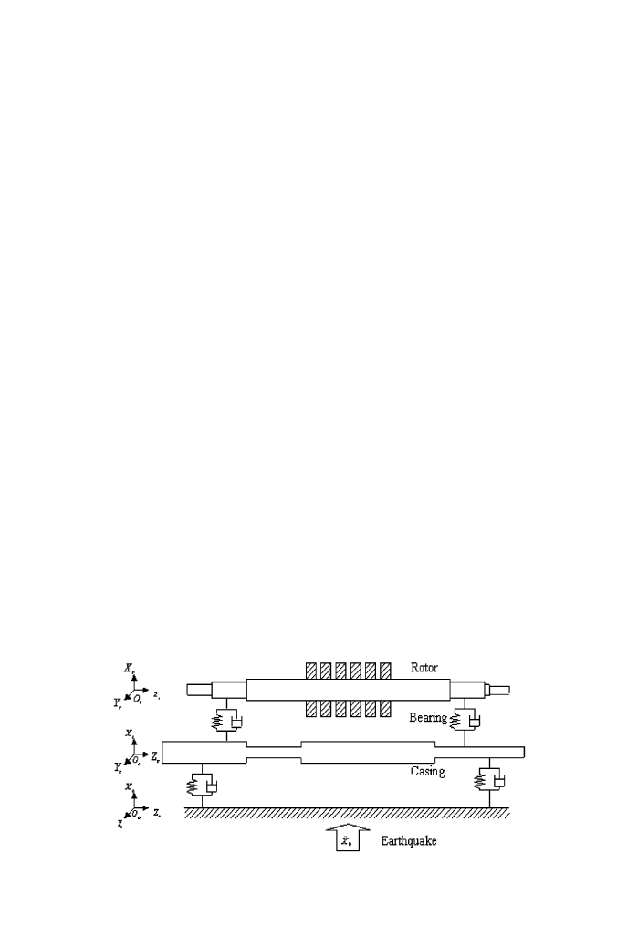
The mechanical structure system with the non-linear restoring force of the system, which

is excited by earthquake, is considered as shown in Figure 1. The excitation is regarded as
a random process; hence, it is extremely difﬁcult to obtain an exact solution. Thus,
solutions can be obtained approximately. It should be noted that the solution itself for
random inputs is not the ultimate goal in stochastic analysis of a non-linear system;
instead, more relevant information is the statistical properties of the amplitude of the
response. To elaborate, a non-linear system with the inputs, which are assumed to be a
Gaussian random process, is considered. Because of the non-linear characteristic, the
output is no longer a Gaussian random process; hence, the statistic characteristic of its
amplitude cannot be evaluated through the PDF (probability density function).

Therefore, an adequate method to evaluate the statistical properties of the response of a

non-linear structure system should be developed. For this reason, the random excitation is
approximated to Gaussian stationary process by reasonable procedures. Then, the non-
linear equation of motion is reinstated with approximated Gaussian process. After that,

Figure 1. Mechanical system for analysis.

B.-Y. MOON AND B.-S. KANG

270

the perturbation theory is applied to solve non-linear equation of motion. Finally, the
statistics properties of nonlinear response are obtained.

2.1.

NON-LINEAR SYSTEM EXCITED BY RANDOM PROCESS

For the simple explanation, equation of motion of the arbitrary mode of non-linear

system can be expressed as

.xx þ 2Bo

’xx þ o

2
0

þ eo

2
0

¼ .

;

ð1Þ

where B

;

are damping ratio and natural frequency respectively. e is a small parameter.

Equation (1) has a non-linear restoring force, which can be expressed in higher order terms
of the displacement, eo

: .

is random excitation, which has a spectrum density S

ðOÞ:

Meaning of the stochastic analysis such as equation (1) is to decide the statistic
information of displacement x. Generally, the statistic characteristic of random process is
decided from the PDF and power spectrum density (PSD) function of the system.
Accordingly, for the probabilistic analysis of non-linear random response, PSD and PDF
of excitation forces should be obtained.

It is clear that ground acceleration is inherently non-stationary, treating a typical record

of earthquake induced ground acceleration [9]. However, if the principal shock duration is
limited to the period corresponding to the strong-motion portion over which the peak
structural response occurs, a stationary process appears to be a good approximation.
Hence, this study deals with the response of a non-linear system under ground excitation
of the stationary random process by considering the strong motion duration of the
earthquake.

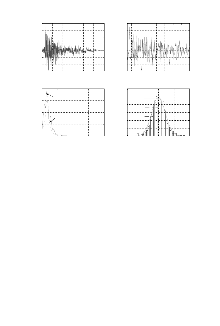
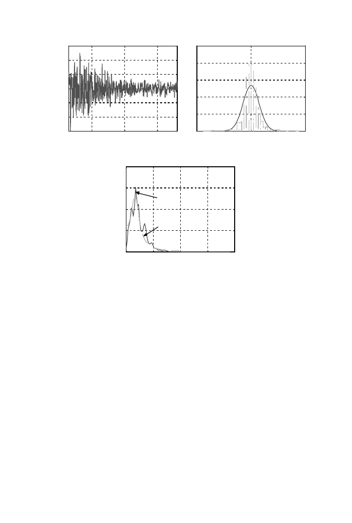
Figure 2 shows the random excitation of the system and its PSD and PDF, which is

regarded as narrow band process. Important values of statistic properties are mean
(=

0072) and peak frequency (=1875 rad/s) and maximum value of acceleration

(175

89 gal). Figure 2(c) shows the corresponding erratic PSD and the ﬁtted PSD function,

which shows relatively good agreement. The computed PSD is obtained from the part of
earthquake data during 3–18 s, which can be regarded as stationary process from the
viewpoint of the amplitude envelope of earthquake graph, as shown in Figure 2(b). The
functional form for the spectral density function of earthquake motion is

ðOÞ ¼

þ4B

;

ð2Þ

where o

;

and S

are a dominant frequency, damping ration of ﬁlter and spectrum

intensity of random process respectively. a is a maximum value of input. Forinstance, Taft
earthquake (1952) has values of B

¼ 041; o

¼ 1875 rad=s; a ¼ 175 m=s

and

0132 m

/sec

respectively. From Figure 2(c), it is estimated that S

ðOÞ can be

applicable to solve the response statistically.

PDF of input is obtained from the part of earthquake data during 0–50 s, during 3–18 s

and during 5–13 s, as shown in Figure 2(d). PDF which is obtained from the part of
earthquake data during 3–18 s shows a reasonable Gaussian distribution. The part of the
earthquake during 3–18 s has the mean (=

00062). Thereby, the strong part of

earthquake excitation process can be regarded as Gaussian stationary random process
with mean zero. The PDF can be expressed as

ð .

Þ ¼

ﬃﬃﬃﬃﬃﬃﬃﬃﬃﬃﬃﬃﬃ

2ps

exp

2
0

;

ð3Þ

SEISMIC RESPONSE ANALYSIS AND RELIABILITY DESIGN

271

where s

;

are the variance of excitation and its root mean square. Then, non-linear

equation of motion can be reinstated as

.xx þ 2Bo

’xx þ o

2
0

þ eo

2
0

¼ W ðtÞ;

ð4Þ

where W(t) is a Gaussian stationary narrow band random process with zero-mean. x(t) is
the stationary response of a linearly damped Dufﬁng system subjected to a Gaussian
process excitation.

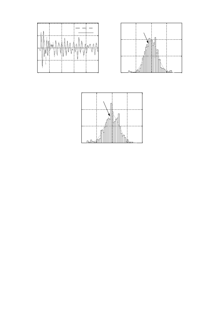
Here, x(t) is not Gaussian process, generally. However, if the system is lightly damped

and if the non-linearity is small (that is, e41), then x(t) is still expected to be a narrow
band random process, as shown in Figure 3, numerical example. The response has the
mean (=

00044). PDF of non-linear response shows a Gaussian distribution. Thus, the

response of Equation (4) can be analyzed statistically by applying the perturbation theory.
In Equation (4), x can be perturbed as x

¼ x

þ ex

This replaces the solution of the non-

linear random vibration problem represented by equation (4) with the solution of a series
of linear random vibration problems with the same differential form but different inputs

.xx

þ 2Bo

’xx

þ o

2
0

¼ W ðtÞ;

ð5Þ

.xx

þ 2Bo

’xx

þ o

2
0

¼ o

2
0

3
0

¼ f

ðx

Þ;

ð6Þ

where f

ðx

Þ ¼ o

3
0

From equations (5) and (6), the approximating functions x(t) can be

obtained sequentially. Here, zeroth order approximation x

is Gaussian process. Its

probabilistic characteristics can be obtained by classical methods of linear random
vibration. However, the characterization of x

is less simple because the input is now a

−

150

−

100

−

100

150

200

Time (sec)

Acceleration(cm/s )

(a)

−

150

−

100

−

100

150

200

Time (sec)

Acceleration(cm/s )

(b)

100

150

200

0. 01

0. 02

0. 03

0. 04

Frequency (rads/sec)

Spectrum (cm /sec

)

Earthquake PSD

PSD function S

(

Ω

)

(c)

−

200

−

100

200

0.002

0.004

0.006

0.008

0.01

0.012

Acceleration (cm/s )

PDF

Gaussian distribution

(1) 0-50 sec

(2) 3-18 sec

(3) 5-13 sec

(d)

Figure 2. Random excitation force and its PSD, PDF. (a) Taft earthquake (1952, S69E), (b) strong part of

earthquake (c) PSD function, (d) PSD function.

B.-Y. MOON AND B.-S. KANG

272

non-Gaussian process whose mean and covariance function are not generally available in
a closed form. Moreover, the determination of the second moment characterization of the
approximate solution x

¼ x

þ ex

also requires the correlation function of x

, x

, which is

not readily available. In handling this problem, the objective is the determination of the
stationary mean and covariance function of the ﬁrst order approximation, as given in
equation (6). Covariance function becomes due to its stationary characteristic

fxðt þ tÞxðtÞg ¼ RðtÞ

¼ Efx

ðt þ tÞx

ðtÞg þ eEfx

ðt þ tÞx

ðtÞg þ eEfx

ðt þ tÞx

ðtÞg; ð7Þ

where each term can be obtained from the random vibration of linear system as

ðt þ tÞx

ðtÞg ¼

fW ðt þ t y

ÞW ðt y

Þghðy

Þhðy

Þ dy

;

ð8Þ

ðt þ tÞx

ðtÞg ¼

fW ðt þ t y

Þf

ðt y

Þghðy

Þhðy

Þ dy

;

ð9Þ

ðt þ tÞx

ðtÞg ¼

fW ðt y

Þf

ðt þ t y

Þghðy

Þhðy

Þ dy

;

ð10Þ

where h(

) is the impulse response function corresponding to e ¼ 0: The determination of

the expectations in equations (8)–(10) involve lengthy but straightforward calculations of

−

Displacement (cm)

Time (sec)

Linear response

Nonlinear response

(a)

−

0.5

1.5

Displacement (cm)

Probability density function

Gaussian distribution

(b)

−

0.5

1.5

Displacement (cm)

Probability density function

Gaussian distribution

(c)

Figure 3. Non-linear response x, linearr

esponse x

and theirPDF (e

¼ 03; B ¼ 01; o¼ 523). (a) Time

response, (b) PDF of non-linear response, (c) PDF of linear response.

SEISMIC RESPONSE ANALYSIS AND RELIABILITY DESIGN

273

expectations of polynomials in Gaussian variables. Thus the covariance function of the
non-linearresponse can be evaluated. Then, the spectral density of the non-linearresponse
is obtained by taking the Fourier transform of equation (7).

ðOÞ ¼ S

ðOÞ HðOÞ

6eo

2
0

2
x

fHðOÞg

;

ð11Þ

where s

is the stationary variance of the linear response. H

ðOÞ is frequency response

function of linearequation between the excitation and the displacement of response. The
corresponding variance can be obtained from the covariance R

ðtÞ of the system by letting

¼ 0; which is the same value of the mean-square response of the non-linear vibration.

Since the mean response, E

½xðtÞ; is zero, the variance is equal to the second moment

E[x(t)]

½x

ðtÞ ¼ Rð0Þ ¼ s

2
x

6eo

2
0

fRðtÞhðtÞg dt

ð12Þ

The mean-square value of the linear response in terms of the system response function and
the spectral density of the input is

2
x

ðOÞ HðOÞ

dO:

ð13Þ

This procedure is applied to analyze a complex M-d.o.f. non-linear system.

2.2.

RELIABILITY ANALYSIS BY CROSSING THEORY

Here, reliability analysis through the crossing theory is considered. Unsatisfactory

performance is assumed to be caused by excessive deformation by a gradual accumulation
of damage under cyclic loading. The reliability of structural systems depends primarily on
crossing characteristics of response process representing deformations. The crossings of
response correspond to crossings of level X of response with positive slope or X-
upcrossings of x(t). The mean X-upcrossing rate of x(t) is

þ
X

ðtÞ ¼ Ef

’xxðtÞ þ jxðtÞ ¼ XgpðX; tÞ;

ð14Þ

where p(X, t), denotes the PDF of

fxðtÞ;

’xxðtÞg; which can be obtained using techniques for

analyzing the response of linear. Note that u

þ
X

ðtÞ ¼ u

þ
X

is time-invariant for stationary

response. The mean X-upcrossing rate of the non-linear displacement x

¼ x

þ ex

can be

obtained as

þ
X

ðtÞ ¼

ﬃﬃﬃ

1=4

8es

exp

8es

exp

;

ð15Þ

where K

1/4

is the modiﬁed Bessel function of order

1
4

2.3.

MODELLING OF A COMPLEX NON-LINEAR STRUCTURE

Forthe analysis, the system shown in Figure 1 is considered as a mechanical system. The

rotor has non-linearity with respect to its material property. For the dynamic analysis of
complex systems, the SSM can be applied. The overall system is divided into three
components, i.e., the rotor is the non-linear component, the casing is the linear
component, and the bearing is the assembling component. The acceleration of gravity is

B.-Y. MOON AND B.-S. KANG

274

ignored for simplicity of analysis. The rotor and casing components are modeled using
ﬁnite element method (FEM).

The co-ordinates of the rotor-bearing-casing system are shown in Figure 1. The O

co-ordinate system is ﬁxed in rotor, such that the origin coincides with the center

of the shaft where the X

-axis is vertically upwards, the Y

-axis is horizontal and

perpendicular to the shaft, and the Z

-axis is along shaft. The O

-X

co-ordinate

system is ﬁxed in casing. The O

-X

is an absolute co-ordinate system, which is ﬁxed

in basement. The U

(=X

, Y

, Z

) is a relative displacement between rotor

and casing. The U

(=X

, Y

, Z

) is a relative displacement between casing

and basement. .

is an acceleration of the earthquake input.

2.4.

MODELLING OF NON-LINEAR COMPONENT

In the current rotating machinery, the non-linear vibration phenomena sometimes occur

in the shrinkage ﬁt rotor, assembly rotor, power plant rotor with coil, and in high polymer
rotor. These phenomena can be modelled with a non-linear restoring force, which can be
expressed in higher order terms of the displacement. To apply the SSM to those complex
system, equation of motion is obtained forthe non-linearcomponent [1–4]. The external
force is considered as the unbalance force and the earthquake. Internal force is considered
because the non-linear component can be synthesized through the internal force with the
othercomponents.

g þ ½

g þ e½K

¼ f

ðtÞg þ f

g þ f

ð16Þ

where

; ½

and ½K

are a mass matrix, stiffness matrix and non-linear stiffness term

respectively.

ðtÞg; f

g are an unbalance excitation of rotor and an internal force

vector. The earthquake force is

g ¼ ½

fIgf .

ð17Þ

where {I} is a vector which shows the direction. In order to apply modal analysis, modal
co-ordinate system

g is introduced by using the modal matrix ½

of the linearsystem.

Then, the displacement

g is transformed into the modal co-ordinate approximately as

[3, 4]

.xxg þ ½

2
n

g þ e½

¼ f

ðtÞg þ f

g þ f

ð18Þ

where

ðtÞg; f

ðtÞg and f

g are an unbalance force, an internal force and an external

force against earthquake in modal co-ordinates respectively.

2
n

;

are an

eigenvalue matrix and a non-linear term in modal co-ordinates.

According to the previous section, the earthquake can be expressed with approximated

Gaussian stationary random process W(t). For the simple expression of external force
equation to describe the SSM method, those external forces are expressed in a term as
f

ðtÞg f

ðtÞg þ f

g: Thus equation (18) can be expressed in a compact form as

.xxg þ ½

2
n

g þ e½

g ¼ f

ðtÞg þ f

ð19Þ

Here, the perturbation method is applied to solve the non-linear equation. The small
variant e can be regarded as the perturbation parameter, because the variant e

SEISMIC RESPONSE ANALYSIS AND RELIABILITY DESIGN

275

small relative to

2
n

: f

g can be expanded in terms of a series of e

g ¼ f

ð0Þ

g þ ef

ð1Þ

g þ . . . ;

ð20Þ

where superscripts (0), (1) denote the perturbation order. Then, the perturbed equations
are evaluated as

.xx

ð0Þ

g þ ½

2
n

ð0Þ

g ¼ f

ð0Þ

g þ f

ð0Þ

.xx

ð1Þ

g þ ½

2
n

ð1Þ

g ¼ f

ð0Þ

Þg þ f

ð1Þ

ð21Þ

where

ð0Þ

Þg ¼ ½

ð0Þ3

ð0Þ

g is external force term, which is expressed in

perturbation zeroth order.

ð0Þ

g and f

ð1Þ

g are perturbed internal forces, which are

obtained from the relation of

g ¼ f

ð0Þ

g þ ef

ð1Þ

g þ :

2.5.

EQUATIONS OF MOTION OF AN ASSEMBLED SYSTEM

To apply the SSM, the casing of rotor system is modelled as linear component and the

equation of motion is obtained readily. After the eigenvalue analysis, the displacement can
be transformed into modal co-ordinate as

g ½

g: ½

; f

g are a modal matrix

and modal co-ordinate of casing. Even the casing is linear system, this component is
perturbed as same as the non-linear component, because the higher order harmonic
oscillation which is occurred in the non-linear component is translated through the higher
order perturbed equation as [4]

.xx

ð0Þ

g þ ½

2
n

ð0Þ

g ¼ f

ð0Þ

g þ f

ð0Þ

.xx

ð1Þ

g þ ½

2
n

ð1Þ

g ¼ f

ð1Þ

ð22Þ

where

ð0Þ

g; f

ð1Þ

g are the perturbed internal forces.

ð2Þ

g is the external force term, which is expressed with approximated Gaussian

stationary random process W

ðtÞ: Though the internal force, equation (22) can be

assembled with equation (21). As an assembling component in SSM, simple linearball
bearings are considered. Generally, there is a damping term in the bearing, but it is ignored
in this study. The restoring force of the bearing is modelled as linear term, where the force
and displacement are expressed as

g ¼ f

g; ½

g ¼ f

ð23Þ

where

ð j ¼ 1; 2Þ are bearing coefﬁcients. f

g; f

g are the internal force vectors of

the non-linearcomponent and linearcomponent r

espectively.

g is a relative

displacement between the rotor and casing corresponding to the bearing. To synthesize
each component through the assembling component, the order of equation is arranged.
The perturbation parameter e of the non-linearcomponent is intr

oduced. Then, the

displacement can be expressed as

g ¼ f

ð0Þ

g þ ef

ð1Þ

ð24Þ

And the internal force vectors are perturbed as

g ¼ f

ð0Þ

g þ e f

ð1Þ

ð25Þ

In SSM, each component is synthesized to entire system. In order to synthesize each

component, equations (21), (22) and (25) are combined and rewritten according to the

B.-Y. MOON AND B.-S. KANG

276

perturbation order e

ðlÞ

ðl ¼ 0; 1Þ:

f.x

ðlÞ

g þ ½ %

ðlÞ

g ¼ fF

ðlÞ

ðtÞg;

ð26Þ

ðlÞ

g ¼ f

ðlÞ

;

ðlÞ

;

ðlÞ

;

ðlÞ

;

fF ðtÞ

ðlÞ

g ¼ f

ðlÞ

;

ðlÞ

;

ðlÞ

;

ðlÞ

and

½ %

ðlÞ

is the stiffness matrix of the overall system, which is composed all of the

component stiffness. According to the synthesizing procedure of SSM, the reduced order
of degrees of freedom for overall system is obtained by modal truncation of each
component. The equation of order e

ðlÞ

is obtained as

.xx

ðlÞ
i

.xx

ðlÞ
i

;

þ ½a

½a

þ ½a

ðlÞ
i

(

)

ðlÞ

(

)

;

ð27Þ

½a

¼ ½f

½f

;

½a

¼ ½f

½f

;

½a

¼ ½f

½f

;

½a

¼ ½f

½f

;

ðlÞ

g; f

ðlÞ

¼ ½f

ð0Þ

;

½f

ð0Þ

where,

½f

is the eigenvector matrix of each component except the assembling region.

½f

is the eigenvector matrix of the assembling region, which is derived from the

eigenvector of each substructure corresponding to its bearing. The external force term of
order e

ð1Þ

is obtained as

ð1Þ

g; f

ð1Þ

¼ ½f

f½

ð0Þ3

gg þ ½f

ð1Þ

g; ½f

f0g þ ½f

ð1Þ

3. EVALUATION OF SYSTEM PERFORMANCE

In this section, the statistical properties of non-linear system vibration are obtained, and

a reliability design is evaluated in a statistical sense.

3.1.

STATISTICAL PROPERTIES OF NON-LINEAR RESPONSE

The response of non-linear random vibration is solved statistically in an overall system.

The earthquake is used as the excitation wave, which is regarded as the Gaussian
stationary random process, by considering the strong motion duration. When the
statistical properties of an earthquake are known, statistical properties of the system
response can be obtained.

After the eigenvalue analysis of the overall system with equation (27), the order e

ðlÞ

co-

ordinate

ðlÞ

g of the overall system is introduced for modal analysis as

ð0Þ

g ½F

ð0Þ

ð1Þ

g ½F

ð1Þ

ð28Þ

where

½F

is the eigenvector matrix of the overall system. The equation of motion of order

ð0Þ

.ZZ

ð0Þ
i

þ 2z

’ZZ

ð0Þ
i

þ o

2
ti

ð0Þ
i

¼ W

ð0Þ

;

ði ¼ 1; 2; 3; . . . ; nÞ;

ð29Þ

SEISMIC RESPONSE ANALYSIS AND RELIABILITY DESIGN

277

where o

is the eigenvalue of the overall system. W

ð0Þ

is the external force term in modal

co-ordinates. The damping of the system is assumed to be the proportional damping of the
eigenvalue. According to the linear random vibration theory, the solution Z

ð0Þ
i

ðtÞ of the

linear differential equation may be readily obtained. Then, the equation of motion of
order e

ð1Þ

can be described as

.ZZ

ð1Þ
i

þ 2zo

’ZZ

ð1Þ
i

þ o

2
ti

ð1Þ
i

¼ f

ð1Þ

ðZ

ð0Þ
i

Þ;

ði ¼ 1; 2; . . . ; nÞ;

ð30Þ

where f

ð1Þ

ðZ

ð0Þ
i

Þð¼ b

2
i

ð0Þ3
i

Þ is the external force term. b

2
i

is the non-linearcoefﬁcient. The

response is

ð1Þ
i

ðtÞ ¼ b

2
i

ð0Þ3
i

ðt tÞh

ðtÞ dt;

ð31Þ

where h

ðtÞ is the impulse response function of the linear system. Accordingly, the response

of a non-linearsystem can be evaluated as

¼ Z

ð0Þ
i

þ eZ

ð1Þ
i

ð32Þ

The equations of Z

ð0Þ
i

;

ð1Þ
i

can be used to compute various statistical properties of the

response. The covariance of the non-linear response, computed to the ﬁrst order of e; can
be obtained as

ðtÞ ¼

1
2

ð0Þ

ðOÞ H

ðOÞ

3
2

ð0Þ2
Zi

ð0Þ

ðOÞ H

ðOÞ

ðOÞcos Ot

dO;

ð33Þ

where H

ðOÞ is conjugate function of H

ðOÞ: S

ð0Þ

ðOÞ is the spectral density of the

excitation. Then, the spectral density S

ðOÞ of the non-linearresponse is obtained by

taking the Fourier transform of the covariance function as

ðS

ðOÞ ¼ S

ð0Þ

ðOÞ H

ðOÞ

6eb

2
i

ð0Þ2
Zi

Re H

ðOÞ

;

ð34Þ

where Re

½H

ðOÞ is the real part of H

ðOÞ: The corresponding variance can be obtained

from the covariance R

ðtÞ of the system by letting t ¼ 0; which is the same value of the

mean-square response of the non-linear vibration

2
Zi

¼ s

ð0Þ2
Zi

6eb

2
i

ðtÞh

ðtÞg dt

ð35Þ

The stationary variance s

ð0Þ2
Zi

is the mean-square value of the linear response. Examining

;

it appears that if the system is non-linear with light damping, weak non-linearity and

the excitation random process is Gaussian stationary, then the response spectral density,
covariance function, and mean-square value, can all be calculated from the knowledge of
the spectral density of the excitation process and the magnitude of the frequency response

ðOÞ

3.2.

RELIABILITY ANALYSIS BY POSSIBILITY OF FAILURE

Generally, the evaluation of seismic response of rotating machinery is concerned with

the maintenance of the operating ability against the seismic excitation. This can be veriﬁed
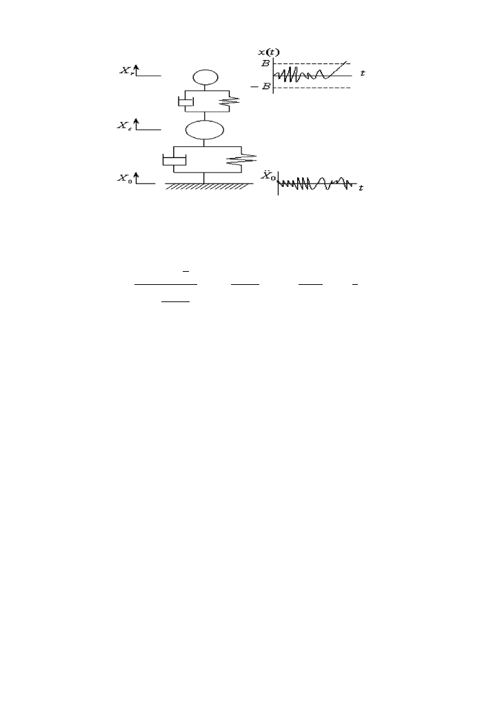
by the possibility of failure by the contact between the bearing and casing. The possibility
of failure is obtained by assuming that a failure of the system occurs when the response
crosses over the safe bound, as shown in Figure 4. The displacement X

is used as the

standard point for the evaluation of the failure problem. The probability that X

exceeds

safe set B gives the probability of the system failure, which is constrained by casing to
prevent the damage of bearing. B is the limited amplitude of the rotor. The mean B-

B.-Y. MOON AND B.-S. KANG

278

upcrossing rate of the non-linear vibration of the system can be obtained as

þ
B

ðtÞ ¼

ð0Þ

ﬃﬃﬃ

1=4

8es

ð0Þ2
Z0

! exp

8es

ð0Þ2

exp

ð0Þ2

;

ð36Þ

where o

is ﬁrst the natural frequency of the overall system. s

ð0Þ2

represents the stationary

variance of ﬁrst modal displacement when

(aa=0. s

ð0Þ

is the root mean square of the

displacement of the ﬁrst modal response.

4. NUMERICAL RESULTS

Numerical calculation results of non-linear stochastic system are obtained under the

random excitation while the system is rotating near the critical speed of the system. Non-
linear characteristics of the random response are observed by the proposed analytical
method and those are compared with the results by the numerical simulation.

4.1.

MODEL FOR ANALYSIS

As an analysis model, a non-linear rotor system, which is shown in Figure 1, is

considered. The rotor is considered as a uniform beam and the casing is also considered as
a uniform beam approximately for the simplicity of calculation. The casing is constrained
to a foundation at both ends of the casing. As a support, ball bearing is considered for
aircraft engine turbine or power plant turbine. The properties of the rotor system are
tabulated in Table 1.

The rotor is modelled by the 20 beam elements and the casing is also modelled by the 20

beam elements. The modal damping ratios of the system is given by z

¼ 005: To check the

computing accuracy of SSM, the natural frequency of the rotor system is calculated by
using FEM, and the results are compared with those calculated by using SSM. The rotor
has 84 d.o.f. because it has 21 nodes and there are 4 variables per mode. The casing also
has 84 d.o.f. so that the total degrees of freedom are 168. Table 2 shows the natural
frequencies of the rotor system calculated by FEM and SSM. In the analysis of SSM, the
numbers of adopted modes in the rotor and casing are changed. The natural frequencies,

Figure 4. Possibility of failure problem.

SEISMIC RESPONSE ANALYSIS AND RELIABILITY DESIGN

279

which are close to the ones by FEM, can be obtained by SSM when the numbers of
adopted modes are increased.

When 20 modes are adopted in the rotor and casing, the error is less than 0

4%. To keep

the accuracy of the lower natural frequencies, it is regarded that 20 modes of both
components are sufﬁcient to this analysis. Thus, 20 modes of each component are adapted
to further response analysis for economic calculation. In the table (A/B), A, B stands for
adopted mode numberfrom the shaft/casing element.

The exciting force of the rotor caused by unbalance is assumed as F

ðtÞ ¼

cos

ðOt þ fÞ in x direction, where F

;

f are unbalance and phase angle, respectively.

Rotating speed (O

¼ 540 rad=s) is assumed to be near ﬁrst critical speed (o

¼ 583 rad=s)

of the rotor system. The unbalance of the rotor system is located at the middle of the shaft
with a value of 0

044 Kg m/(rad/s)

4.2.

RESPONSE OF THE NON-LINEAR SYSTEM

First, the linear response of the system against the random excitation is examined. The

responses are computed by SSM with modal analysis procedure, which are shown in
Figure 5. The statistic properties of the system response are examined. As can be noticed
from Figure 5(a), the response includes the earthquake response of the system. Probability
density of the system is shown in Figure 5(b) in accordance with relative amplitude of the
system. Average value of response is 0

000186, which shows almost zero mean. These

properties prove that the response is Gaussian stationary random process. In Figure 5(c),
the power spectrum of the response is shown. It can be observed that a typical earthquake
response power spectrum is obtained, which has a low-frequency component. Spectrum
shows the fact that response is in a short period and predominant frequency is in a lower
frequency where the peak frequency of the response is 28

27 rad/s. The simulated PSD

shows well ﬁtted with the analytical response of PSD S

ðOÞ; which is obtained when e ¼ 0:

Table 1

Properties of the rotor system

Rotor, casing length (mm)

800

Rotordiameter(mm)

Casing diameter(mm)

Young’s modulus (N/m

)

1 10

Density of rotor and casing (kg/m

)

81 10

Bearing coefﬁcient (N/m)

0 10

Constrain coefﬁcient (N/m)

0 10

Table 2

Natural frequency of rotor system (Hz)

Mode No.

FEM

SSM

168 (d.o.f.)

12/12

20/20

40/40

164

162

164

B.-Y. MOON AND B.-S. KANG

280

The spectral density is related to the stationary variance s

ð0Þ2

¼ 00059; which is the same

as the mean-square value of the linear response.

Here, the statistical properties of non-linear random vibration of the stochastic system

versus the strong motion duration of excitation are investigated. Correlation, spectrum
density and its variances, which are important to reliability analysis, are considered. Those
properties of non-linear responses are calculated according to the procedure of non-linear
random vibration analysis, which is computed to the perturbation ﬁrst order. Spectrum of
harmonic excitation and earthquake excitation are obtained and applied to the system. If
the dual inputs are uncorrelated, then the cross-spectral density function of earthquake
and unbalance excitation terms in the equation of spectral density become zero. Then, the
autocorrelation and the spectral density of the non-linear response are obtained
theoretically. It is regarded that the non-linear response depends on the size of the
perturbation parameter, which shows nonlinear characteristics. To this end, two kinds of
analysis are carried out, i.e., the perturbation parameters are set to e

¼ 02; 05. In Figure 6,

the PSD of the non-linearresponses of the system at the middle of shaft and casing is
shown with various non-linear parameters. The response of SSM is calculated by taking 20
modes. When the non-linearparameteris e

¼ 00; the PSD is equal to a linearresponse.

The each PSD of the system, such as rotor and casing, shows a characteristic of
earthquake random process. Investigation of the PSD reveals that the PSD is smaller when

−

1.5

−

0.5

1.5

x 10

−

Time (sec)

Displacement (m)

−

0.5

Displacement (m)

Gaussian distribution

100

150

200

0.5

1.5

x 10

−

Frequency (rad/s)

Spectrum Density

Computed PSD

Fitted PSD S

(

Ω

)

(a)

(b)

(c)

Figure 5. Linear response and its probabilistic properties. (a) Response of rotor, (b) Gaussian distribution,

SEISMIC RESPONSE ANALYSIS AND RELIABILITY DESIGN

281

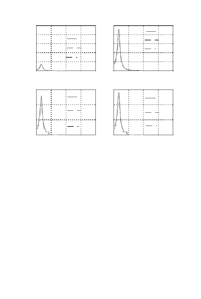
the perturbation parameter becomes bigger, which shows the non-linear characteristic of
response. In the ﬁgure, (L), (C) stand forthe left end nodal point and centerof model.

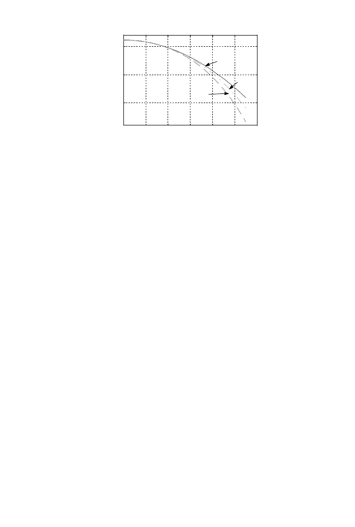
Variance of the non-linear response, which is important value of reliability analysis in

stochastic system, is evaluated from the non-linear response. Figure 7(a) shows the
variance of the non-linear response at the middle of rotor by changing its numbers of
adopting modes 20, 40. The calculated variances are investigated for various values of
non-linear parameter. To prove the computing efﬁciency, those values are compared with
the results of simulation, which is obtained with same calculation condition. The response
of simulation is calculated by direct integration of the equation of motion against the
excitation where the overall equation of motion of the system has 168 d.o.f. Investigation
of the variance reveals that the value shows a decrease with e in the spread of displacement
about equilibrium point when e

¼ 0: This is consistent with ourintuition, which suggests

that stiffersystems exhibit smallerdisplacements, and with the observation that the system
stiffness increases with non-linear parameter. This result also reveals that the variance
displacement of a hardening spring non-linear system is always less than that for the
corresponding linear system.

Figure 7(b) shows the variance of the non-linear response at the middle of rotor by using

its numbers of adopting mode 20. The calculated variances are investigated for various
values of non-linear parameter against maximum values of exciting acceleration. To prove
the non-linear effect, those values are compared with the results of linear one, which is
obtained by same calculation condition. It is observed that according to the input level,

100

150

200

0.2

0.4

0.6

0.8

x 10

−

frequency (rad/sec)

Spectrum density

=0.0

=0.2

=0.5

100

150

200

0.2

0.4

0.6

0.8

x 10

−

frequency (rad/sec)

Spectrum density

=0.0

=0.2

=0.5

100

150

200

0.5

1.5

x 10

−

frequency (rad/sec)

Spectrum density

=0.0

=0.2

=0.5

100

150

200

0.5

1.5

x 10

−

frequency (rad/sec)

Spectrum density

=0.0

=0.2

=0.5

(a)

(b)

(d)

(c)

Figure 6. Comparing PSD of the responses. (a) Spectrum of rotor response (L), (b) spectrum of rotor response

(C), (c) spectrum of casing response (L), (d) spectrum of casing response (C).

B.-Y. MOON AND B.-S. KANG

282

variance of the responses become large. When the non-linear parameters become large,
then the response changes a lot.

Next, the computing time is compared to analyze the non-linear random vibration

versus the strong motion duration (=3–18 s) of excitation. The variances of response for
the values to be compared are used, as shown in Figure 7(a). The computer used in this
analysis is a LOGIX, IBM personal computer. In the case of the numerical simulation, it
takes 20 min 45 s. But forthe proposed method; it takes 5 min 28 s, 7 min 30 s to obtain the
result, when the number of adopting modes are 20, 40 respectively. As a result, it can be
shown that a drastic reduction in calculation time can be achieved, keeping its computing
accuracy. This is an important factor in the analysis of structural dynamics against
random excitation with a large number of degrees of freedom.

4.3.

FAILURE POSSIBILITY

Reliability of the system can be obtained by supposing that the failure of the system

occurs when the system exceeds the limit amplitude. To consider this, the limit of response
(B) at rotor is regarded, which is constrained by casing to prevent the damage of bearing.
This condition can be used to deﬁne a safe set. In this case, performance of the system
depends primarily on crossing characteristics of safe set of response. Thus, the concept for
mean crossing rate of safe set is applied to demonstrate the reliability of the system, as
shown in Figure 8.

Figure 8 shows mean upcrossing rates of stationary non-linear responses for several

values of non-linear parameter. The mean upcrossing rate decreases with threshold B due
to a rapid reduction of probability density of the process reaching B. The mean upcrossing
rate decreases more when non-linear parameters become large. These rates of the non-
linear response can be used to approximate and bound the probability that the response or
the restoring force does not exceed critical values of system. The reliability coincides with
the mean upcrossing rate that the response belongs to the safe set. Also, the probability of
failure can be obtained by the complement of obtained reliability.

0.2

0.4

0.6

0.8

−

1.5

−

0.5

x 10

−

Nonlinear parameter (

)

Log(

(0))

Log(

(0))

SSM(20 modes)

SSM(40 modes)

Simulation

0.5

1.5

−

x 10

−

Acceleration

(m/sec

)

=0.0

=0.2

=0.5

(a)

(b)

Figure 7. Displacement variance of the system. (a) Variance with non-linear parameter e, (b) variance with

acceleration a.

SEISMIC RESPONSE ANALYSIS AND RELIABILITY DESIGN

283

5. CONCLUSIONS

In this paper, the random vibration analysis method of a non-linear stochastic system

was theoretically formulated when the actual random excitation is regarded as a Gaussian
stationary random process. The formulation is concerned with reducing the number of
degrees of freedom for each component by modal substitution. All of the components are
then assembled together and the random response of the overall system is analyzed
statistically against earthquake excitation. It is shown that non-linear random responses
could be efﬁciently calculated according to the selected number of vibration modes.
Several statistical properties of the random responses that are of interest in non-linear
random vibration applications are reviewed. The variance value of the non-linear random
response is obtained economically, which is important in evaluating the reliability of the
system. The results reported herein provide a better understanding of the non-linear
random vibration. Moreover, it is believed that those properties of the results can be
utilized in the dynamic design of the non-linearstochastic system.

ACKNOWLEDGMENTS

This work was supported in part by Brain Korea 21 Program.

REFERENCES

1. T. Iwatsubo, S. Kawamura and B. Moon 1988 JSME International Journal Series III 41,

727–733. Non-linear vibration analysis of rotor system using substructure synthesis method
(Analysis with consideration of non-linearity of rotor)’’.

2. T. Iwatsubo, K. Shimbo, S. Kawamura and B.-Y. Moon 1999 Transactions of the Japanese

Society of Mechanical Engineers Series C 65, 3499–3506. (in Japanese) Non-linearvibration
analysis of rotor system using component mode synthesis method (Analysis using the
perturbation method).

3. B.-Y. Moon, J.-W. Kim and B.-S. Yang 1999 KSME International Journal 13, 620–629. Non-

linear vibration analysis of mechanical structure system using substructure synthesis method.

4. B.-Y. Moon and B. Kang 2001 JSME International Journal Series III 44, 12–20. Non-linear

vibration analysis of rotor system using substructure synthesis method (Analysis with
consideration of nonlinear sensitivity).

0.2

0.4

0.6

0.8

1.2

−

=0.0

=0.2

=0.5

Log(

)

Level of response B(mm)

Figure 8. Mean B-upcrossing rate of response.

B.-Y. MOON AND B.-S. KANG

284

5. A. H. Soni and V. Srinivasan 1983 Transactions of the American Society of Mechanical

Engineers, Journal of Vibration, Acoustics, Stress and Reliability in Design 105, 489–455. Seismic
analysis of a gyroscopic mechanical system.

6. V. Srinivasan and A.H. Soni, 1983 Journal of Earthquake Engineering and Structure Dynamic

12, 287–311. Seismic analysis of a rotor bearing system.

7. O. Matsushita, M. Takagi and K. Kikuchi, 1983 Transactions of the Japanese Society of

Mechanical Engineers Series C 49, 971–981. (in Japanese). Seismic analysis of a rotor system.

8. T. Azuma and S. Saito, 1984 Transactions of the Japanese Society of Mechanical Engineers

Series C 50, 2242–2248. (in Japanese). Seismic analysis of a rotor system using complex modal
method.

9. T.T Soong and M. Grigoriu Random Vibration of Mechanical and Structural Systems, PTR

Prentice Hall, Englewood Cliffs, pp. 64–65.

SEISMIC RESPONSE ANALYSIS AND RELIABILITY DESIGN

285

Document Outline

1. INTRODUCTION
2. METHOD OF ANALYSIS
3. EVALUATION OF SYSTEM PERFORMANCE
- Figure 4
4. NUMERICAL RESULTS
- TABLE 1
- TABLE 2
- Figure 5
- Figure 6
- Figure 7
- Figure 8
5. CONCLUSIONS
ACKNOWLEDGMENTS
REFERENCES

Statistical seismic response analysis and reliability design of nonlinear structure system

Document Outline