arXiv:cs.CG/0203026 v1 22 Mar 2002

Conformal geometry, Euclidean space

and geometric algebra

Chris Doran

1

, Anthony Lasenby

2

and Joan Lasenby

3

Cambridge University, UK

Abstract

Projective geometry provides the preferred framework for most imple-

mentations of Euclidean space in graphics applications. Translations and
rotations are both linear transformations in projective geometry, which
helps when it comes to programming complicated geometrical operations.
But there is a fundamental weakness in this approach — the Euclidean
distance between points is not handled in a straightforward manner. Here
we discuss a solution to this problem, based on conformal geometry. The
language of geometric algebra is best suited to exploiting this geometry, as
it handles the interior and exterior products in a single, unified framework.
A number of applications are discussed, including a compact formula for
reflecting a line off a general spherical surface.

Keywords: geometric algebra, Clifford algebra, conformal geometry, projective

geometry, homogeneous coordinates, sphere geometry, stereographic projection

1

Introduction

In computer graphics programming the standard framework for modeling points
in space is via a projective representation. So, for handling problems in three-
dimensional geometry, points in Euclidean space x are represented projectively
as rays or vectors in a four-dimensional space,

X = x + e

4

.

(1)

The additional vector e

4

is orthogonal to x, e

4

· x = 0, and is normalised to

1, (e

4

)

2

= 1. From the definition of X it is apparent that e

4

is the projective

representation of the origin in Euclidean space. The projective representation
is homogeneous, so both X and λX represent the same point. Projective space
is also not a linear space, as the zero vector is excluded. Given a vector A in
projective space, the Euclidean point a is then recovered from

a =

A − A·e

4

e

4

A·e

4

.

(2)

The components of A define a set of homogeneous coordinates for the position
a.

The advantage of the projective framework is that the group of Euclidean

transformations (translations, reflections and rotations) is represented by a set

1

e-mail: [e-mail]

2

e-mail: [e-mail]

3

e-mail: [e-mail]

1

of linear transformations of projective vectors. For example, the Euclidean
translation x 7→ x + a is described by the matrix transformation







1 0

0 a

1

0 1

0 a

2

0 0

1 a

3

0 0

0

1













x

1

x

2

x

3

1







=







x

1

+ a

1

x

2

+ a

2

x

3

+ a

3

1







.

(3)

This linearisation of a translation ensures that compounding a sequence of trans-
lations and rotations is a straightforward exercise in projective geometry. All
one requires for applications is a fast engine for multiplying together 4 × 4 ma-
trices.

The main operation in projective geometry is the exterior product, originally

introduced by Grassmann in the nineteenth century [1, 2]. This product is
denoted with the wedge symbol ∧. The outer product of vectors is associative
and totally antisymmetric. So, for example, the outer product of two vectors A
and B is the object A∧B, which is a rank-2 antisymmetric tensor or bivector.
The components of A∧B are

(A∧B)

ij

= A

i

B

j

− A

j

B

i

.

(4)

The exterior product defines the join operation in projective geometry, so the
outer product of two points defines the line between them, and the outer product
of three points defines a plane. In this scheme a line in three dimensions is then
described by the 6 components of a bivector. These are the Pl¨

ucker coordinates

of a line. The associativity and antisymmetry of the outer product ensure that

(A∧B)∧(A∧B) = A∧B ∧A∧B = 0,

(5)

which imposes a single quadratic condition on the coordinates of a line. This is
the Pl¨

ucker condition.

The ability to handle straight lines and planes in a systematic manner is

essential to practically all graphics applications, which explains the popularity
of the projective framework. But there is one crucial concept which is miss-
ing. This is the Euclidean distance between points. Distance is a fundamental
concept in the Euclidean world which we inhabit and are usually interested in
modeling. But distance cannot be handled elegantly in the projective frame-
work, as projective geometry is non-metrical. Any form of distance measure
must be introduced via some additional structure. One way to proceed is to
return to the Euclidean points and calculate the distance between these directly.
Mathematically this operation is distinct from all others performed in projective
geometry, as it does not involve the exterior product (or duality). Alternatively,
one can follow the route of classical planar projective geometry and define the
additional metric structure through the introduction of the absolute conic [3].
But this structure requires that all coordinates are complexified, which is hardly
suitable for real graphics applications. In addition, the generalisation of the ab-
solute conic to three-dimensional geometry is awkward.

There is little new in these observations. Grassmann himself was dissatisfied

with an algebra based on the exterior product alone, and sought an algebra of
points where distances are encoded in a natural manner. The solution is pro-
vided by the conformal model of Euclidean geometry, originally introduced by

2

M¨obius in his study of the geometry of spheres. The essential new feature of
this space is that it has mixed signature, so the inner product is not positive
definite. In the nineteenth century, when these developments were initiated,
mixed signature spaces were a highly original and somewhat abstract concept.
Today, however, physicists and mathematicians routinely study such spaces in
the guise of special relativity, and there are no formal difficulties when com-
puting with vectors in these spaces. As a route to understanding the conformal
representation of points in Euclidean geometry we start with a description of the
stereographic projection

. This map provides a means of representing points as

null vectors in a space of two dimensions higher than the Euclidean base space.
This is the conformal representation. The inner product of points in this space
recovers the Euclidean distance, providing precisely the framework we desire.
The outer product extends the range of geometric primitives from projective
geometry to include circles and spheres, which has many applications.

The conformal model of Euclidean geometry makes heavy use of both the

interior and exterior products. As such, it is best developed in the language
of geometric algebra — a universal language for geometry based on the math-
ematics of Clifford algebra [4, 5, 6]. This is described in section 3. The power
of the geometric algebra development becomes apparent when we discuss the
group of conformal transformations, which include Euclidean transformations as
a subgroup. As in the projective case, all Euclidean transformations are linear
transformations in the conformal framework. Furthermore, these transforma-
tions are all orthogonal, and can be built up from primitive reflections.

The join operation in conformal space generalises the join of projective ge-

ometry. Three points now define a line, which is the circle connecting the
points. If this circle passes through the point at infinity it is a straight line.
Similarly, four points define a sphere, which reduces to a plane when its radius
is infinite. These new geometric primitives provide a range of intersection and
reflection operations which dramatically extend the available constructions in
projective geometry. For example, reflecting a line in a sphere is encoded in a
simple expression involving a pair of elements in geometric algebra. Working
in this manner one can write computer code for complicated geometrical oper-
ations which is robust, elegant and highly compact. This has many potential
applications for the graphics industry.

2

Stereographic projection and conformal space

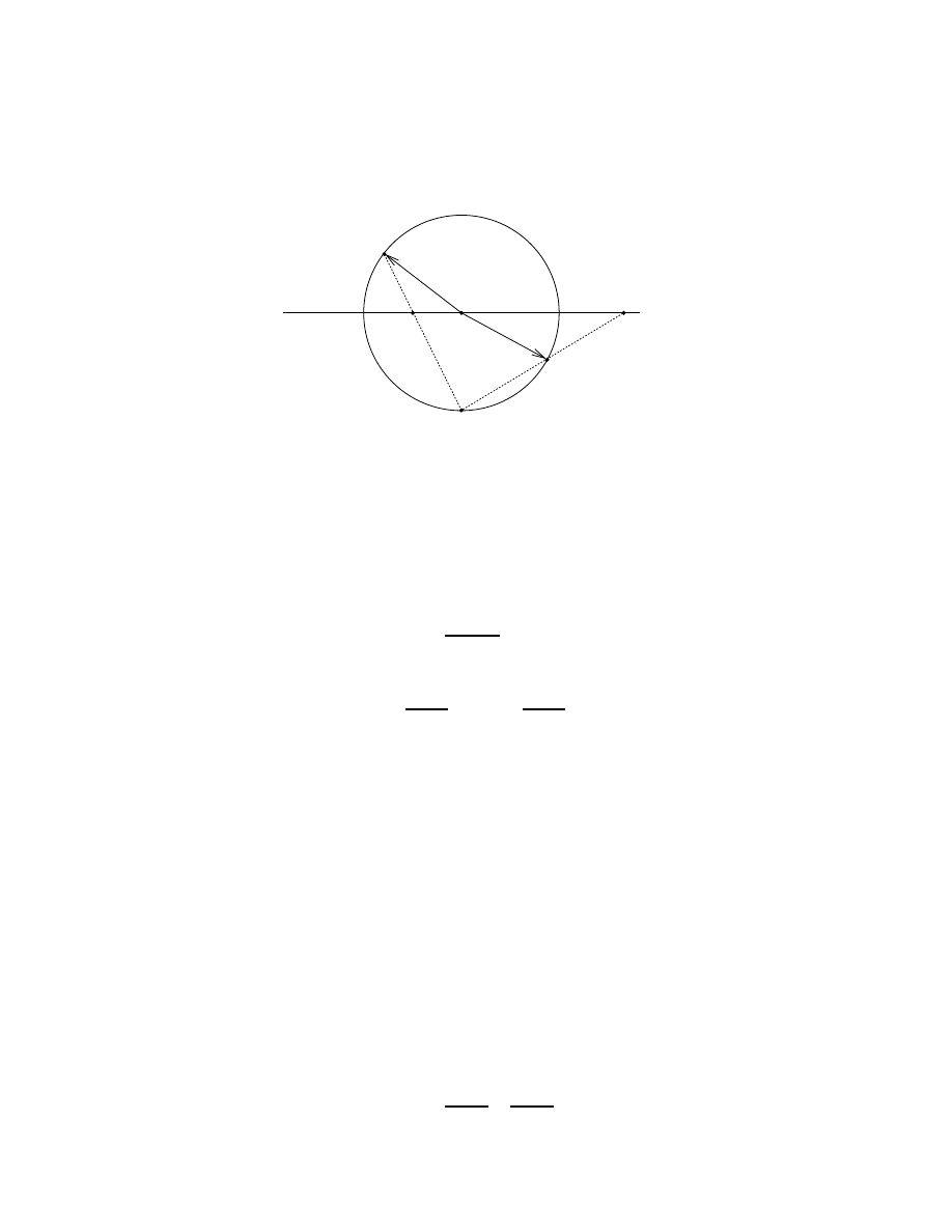
The stereographic projection provides a straightforward route to the principle
construction of the conformal model — the representation of a point as a null
vector in conformal space. The stereographic projection maps points in the
Euclidean space R

n

to points on the unit sphere S

n

, as illustrated in figure 1.

Suppose that the initial point is given by x ∈ R

n

, and we write

x = rˆ

x,

(6)

where r is the magnitude of the vector x, r

2

= x

2

. The corresponding point on

the sphere is

S(x) = cosθ ˆ

x − sinθ e,

(7)

3

y

S(y)

S(x)

x

Figure 1: A stereographic projection. The space R

n

is mapped to the unit sphere

S

n

. Given a point in R

n

we form the line through this point and the south pole

of the sphere. The point where this line intersects the sphere defines the image
of the projection.

where e is the unit vector perpendicular to the plane defining the south pole of
the sphere S

n

. The angle θ, −π/2 ≤ θ ≤ π/2 is related to the distance r by

r =

cosθ

1 + sinθ

,

(8)

which inverts to give

cos θ =

2r

1 + r

2

,

sin θ =

1 − r

2

1 + r

2

.

(9)

The stereographic projection S maps R

n

into S

n

− P , where P is the south pole

of S

n

. We complete the space S

n

by letting the south pole represent the point

at infinity. We therefore expect that, under Euclidean transformations of R

n

,

the point at infinity should remain invariant.

We now have a representation of points in R

n

with unit vectors in the space

R

n+1

. But the constraint that the vector has unit magnitude means that this

representation is not homogeneous. A homogeneous representation of geometric
objects is critical to the power of projective geometry, as it enables us to write
the equation of the line through A and B as

A∧B ∧X = 0.

(10)

Clearly, if X satisfies this equation, then so to does λX. To achieve a ho-
mogeneous representation we introduce a further vector, ¯

e, which has negative

signature

,

¯

e

2

= −1.

(11)

We also assume that ¯

e is orthogonal to x and e. We can now replace the unit

vector S(x) with the vector X, where

X = S(x) + ¯

e =

2x

1 + x

2

−

1 − x

2

1 + x

2

e + ¯

e.

(12)

4

The vector X satisfies

X ·X = 0

(13)

so is null. This equation is homogeneous, so we can now move to a homoge-
neous encoding of points and let X and λX represent the same point in R

n

.

Multiplying the vector in equation (12) by (1 + x

2

) we establish the conformal

representation

F (x) = X = 2x − (1 − x

2

)e + (1 + x

2

)¯

e.

(14)

The vectors e and ¯

e extend the Euclidean space R

n

to a space with two extra

dimensions and signature (n + 1, 1). It is generally more convenient to work
with a null basis for the extra dimensions, so we define

n = e + ¯

e

¯

n = e − ¯

e.

(15)

These vectors satisfy

n

2

= ¯

n

2

= 0,

n· ¯

n = 2.

(16)

The vector X is now

F (x) = X = 2x + x

2

n − ¯

n,

(17)

which defines our standard representation of points as vectors in conformal
space. Given a general, unnormalised null vector in conformal space, the stan-
dard form of equation (17) is recovered by setting

X 7→ −2

X

X ·n

.

(18)

This map makes it clear that the null vector n now represents the point at
infinity. In general we will not assume that our points are normalised, so the
components of X are homogeneous coordinates for the point x. The step of
normalising the representation is only performed if the actual Euclidean point
is required.

Given two null vectors X and Y , in the form of equation (17), their inner

product is

X ·Y = x

2

n + 2x − ¯

n

· y

2

n + 2y − ¯

n

= −2x

2

− 2y

2

+ 4x·y

= −2(x − y)

2

.

(19)

This is the key result which justifies the conformal model approach to Euclidean
geometry. The inner product in conformal space encodes the distance between
points in Euclidean space. This is why points are represented with null vectors
— the distance between a point and itself is zero. Since equation (19) was
appropriate for normalised points, the general expression relating Euclidean
distance to the conformal inner product is

|x − y|

2

= −2

X ·Y

X ·n Y ·n

.

(20)

5

This is manifestly homogeneous in X and Y . This formula returns the dimen-
sionless distance. To introduce dimensions one requires a fundamental length
scale λ, so that x is the dimensionless representation of the position vector λx.
Appropriate factors of λ can then be inserted when required.

An orthogonal transformation in conformal space will ensure that a null

vector remains null. Such a transformation therefore maps points to points in
Euclidean space. This defines the full conformal group of Euclidean space, which
is isomorphic to the group SO(n + 1, 1). Conformal transformations leave angles
invariant, but can map straight lines into circles. The Euclidean group is the
subgroup of the conformal group which leaves the Euclidean distance invariant.
These transformations include translations and rotations, which are therefore
linear, orthogonal transformations in conformal space. The key to developing
simple representations of conformal transformations is geometric algebra, which
we now describe.

3

Geometric algebra

The language of geometric algebra can be thought of as Clifford algebra with
added geometric content. The details are described in greater detail elsewhere
[4, 5, 6], and here we just provide a brief introduction. A geometric algebra
is constructed on a vector space with a given inner product. The geometric
product of two vectors a and b is defined to be associative and distributive over
addition, with the additional rule that the (geometric) square of any vector is
a scalar,

aa = a

2

∈ R.

(21)

If we write

ab + ba = (a + b)

2

− a

2

− b

2

(22)

we see that the symmetric part of the geometric product of any two vectors is
also a scalar. This defines the inner product, and we write

a·b =

1
2

(ab + ba).

(23)

The geometric product of two vectors can now be written

ab = a·b + a∧b,

(24)

where the exterior product is the antisymmetric combination

a∧b =

1
2

(ab − ba).

(25)

Under the geometric product, orthogonal vectors anticommute and parallel vec-
tors commute. The product therefore encodes the basic geometric relationships
between vectors. The totally antisymmetrised sum of geometric products of
vectors defines the exterior product in the algebra.

Once one knows how to multiply together vectors it is a straightforward

exercise to construct the entire geometric algebra of a vector space. General
elements of this algebra are called multivectors, and they too can be multiplied

6

via the geometric product. The two algebras which concern us in this paper are
the algebras of conformal vectors for the Euclidean plane and three-dimensional
space [7, 8, 9]. For the Euclidean plane, let {e

1

, e

2

} denote an orthonormal basis

set, and write e

0

= ¯

e, e

3

= e. The full basis set is then {e

i

}, i = 0 . . . 3. These

generators satisfy

e

i

e

j

+ e

j

e

i

= 2η

ij

,

i, j = 0 . . . 3,

(26)

where

η

ij

= diag(−1, 1, 1, 1).

(27)

The algebra generated by these vectors consists of the set

1

{e

i

}

{e

i

∧e

j

}

{Ie

i

}

I

1 scalar 4 vectors 6 bivectors 4 trivectors 1 pseudoscalar.

Scalars are assigned grade zero, vectors grade one, and so on. The highest grade
term in the algebra is the pseudoscalar I,

I = e

0

e

1

e

2

e

3

= e

1

e

2

¯

ee.

(28)

This satisfies

I

2

= e

1

e

2

¯

eee

1

e

2

¯

ee = −e

1

e

2

¯

ee

1

e

2

¯

e = e

1

e

2

e

1

e

2

= −e

1

e

1

= −1.

(29)

The steps in this calculation simply involve counting the number of sign changes
as a vector is anticommuted past orthogonal vectors. This is essentially how
all products in geometric algebra are calculated, and it is easily incorporated
into any programming language. In even dimensions, such as the case here, the
pseudoscalar anticommutes with vectors,

Ia = −aI,

even dimensions.

(30)

For the case of the conformal algebra of Euclidean three-dimensional space

R

3

, we can define a basis as {e

i

}, i = 0 . . . 4, with e

0

= ¯

e, e

4

= e, and e

i

, i =

1 . . . 3 a basis set for three-dimensional space. The algebra generated by these
vectors has 32 terms, and is spanned by

1

{e

i

}

{e

i

∧e

j

}

{e

i

∧e

j

∧e

k

} {Ie

i

}

I

grade 0

1

2

3

4

5

dimension 1

5

10

10

5

1.

The dimensions of each subspace are given by the binomial coefficients. Each
subspace has a simple geometric interpretation in conformal geometry. The
pseudoscalar for five-dimensional space is again denoted by I, and this time is
defined by

I = e

0

e

1

e

2

e

3

e

4

= e

1

e

2

e

3

e¯

e.

(31)

In five-dimensional space the pseudoscalar commutes with all elements in the
algebra. The (4, 1) signature of the space implies that the pseudoscalar satisfies

I

2

= −1.

(32)

So, algebraically, I has the properties of a unit imaginary, though in geometric
algebra it plays a definite geometric role. In a general geometric algebra, mul-
tiplication by the pseudoscalar performs the duality transformation familiar in
projective geometry.

7

4

Reflections and rotations in geometric algebra

Suppose that the vectors a and m represent two lines from a common origin in
Euclidean space, and we wish to reflect the vector a in the hyperplane perpen-
dicular to m. If we assume that m is normalised to m

2

= 1, the result of this

reflection is

a 7→ a

0

= a − 2(a·m)m.

(33)

This is the standard expression one would write down without access to the
geometric product. But with geometric algebra at our disposal we can expand
a

0

into

a

0

= a − (am + ma)m = a − am

2

− mam = −mam.

(34)

The advantage of this representation of a reflection is that we can easily chain
together reflections into a series of geometric products. So two reflections, one
in m followed by one in l, produce the transformation

a 7→ lmaml.

(35)

But two reflections generate a rotation, so a rotation in geometric algebra can
be written in the simple form

a 7→ Ra ˜

R

(36)

where

R = lm,

˜

R = ml.

(37)

The tilde denotes the operation of reversion, which reverses the order of vectors
in any series of geometric products. Given a general multivector A we can
decompose it into terms of a unique grade by writing

A = A

0

+ A

1

+ A

2

+ · · · ,

(38)

where A

r

denotes the grade-r part of A. The effect of the reverse on A is then

˜

A = A

0

+ A

1

− A

2

− A

3

+ A

4

+ · · · .

(39)

The geometric product of an even number of positive norm unit vectors is called
a rotor. These satisfy R ˜

R = 1 and generate rotations. A rotor can be written

as

R = ± exp(B/2)

(40)

where B is a bivector. The space of bivectors is therefore the space of generators
of rotations. These define a Lie algebra, with the rotors themselves defining a
Lie group

. The action of this group on vectors is defined by equation (36), so

both R and −R define the same rotation.

8

5

Euclidean and conformal transformations

Transformations of conformal vectors which leave the product of equation (20)
invariant correspond to the group of Euclidean transformations in R

n

. To sim-

plify the notation, we let G(p, q) denote the geometric algebra of a vector space
with signature (p, q). The Euclidean spaces of interest to us therefore have the
algebras G(2, 0) and G(3, 0) associated with them. The corresponding confor-
mal algebras are G(3, 1) and G(4, 1) respectively. Each Euclidean algebra is a
subalgebra of the associated conformal algebra.

The operations which mainly interest us here are translations and rotations.

The fact that translations can be treated as orthogonal transformations is a
novel feature of conformal geometry. This is possible because the underlying
orthogonal group is non-compact, and so contains null generators. To see how
this allows us to describe a translation, consider the rotor

R = T

a

= e

na/2

(41)

where a is a vector in the Euclidean space, so that a · n = 0. The bivector
generator satisfies

(na)

2

= −anna = 0,

(42)

so is null. The Taylor series for T

a

therefore terminates after two terms, leaving

T

a

= 1 +

na

2

.

(43)

The rotor T

a

transforms the null vectors n and ¯

n into

T

a

n ˜

T

a

= n +

1
2

nan +

1
2

nan +

1
4

nanan = n

(44)

and

T

a

¯

n ˜

T

a

= ¯

n − 2a − a

2

n.

(45)

As expected, the point at infinity remains at infinity, whereas the origin is
transformed to the vector a. Acting on a vector x ∈ G(n, 0) we similarly obtain

T

a

x ˜

T

a

= x + n(a·x).

(46)

Combining these results we find that

T

a

F (x) ˜

T

a

= x

2

n + 2(x + a·x n) − (¯

n − 2a − a

2

n)

= (x + a)

2

n + 2(x + a) − ¯

n

= F (x + a),

(47)

which performs the conformal version of the translation x 7→ x+ a. Translations
are handled as rotations in conformal space, and the rotor group provides a
double-cover representation of a translation. The identity

˜

T

a

= T

−a

(48)

ensures that the inverse transformation in conformal space corresponds to a
translation in the opposite direction, as required.

9

Similarly, as discussed above, a rotation in the origin in R

n

is performed by

x 7→ x

0

= Rx ˜

R, where R is a rotor in G(n, 0). The conformal vector representing

the transformed point is

F (x

0

) = (x

0

)

2

n + 2Rx ˜

R − ¯

n

= R(x

2

n + 2x − ¯

n) ˜

R = RF (x) ˜

R.

(49)

This holds because R is an even element in G(n, 0), so must commute with
both n and ¯

n. Rotations about the origin therefore take the same form in either

space. But suppose instead that we wish to rotate about the point a ∈ R

n

. This

can be achieved by translating a to the origin, rotating, and then translating
forward again. In terms of X = F (x) the result is

X 7→ T

a

RT

−a

X ˜

T

−a

˜

R ˜

T

a

= R

0

X ˜

R.

(50)

The rotation is now controlled by the rotor R

0

, where

R

0

= T

a

R ˜

T

a

=

1 +

na

2

R

1 +

an

2

.

(51)

The conformal model frees us up from treating the origin as a special point.
Rotations about any point are handled with rotors in the same manner. Similar
comments apply to reflections, though we will see shortly that the range of
possible reflections is enhanced in the conformal model. The Euclidean group is
a subgroup of the full conformal group, which consists of transformations which
preserve angles alone. This group is described in greater detail elsewhere [5, 9].
The essential property of a Euclidean transformation is that the point at infinity
is invariant, so all Euclidean transformations map n to itself.

6

Geometric primitives in conformal space

In the conformal model, points in Euclidean space are represented homoge-
neously by null vectors in conformal space. As in projective geometry, a multi-
vector L ∈ G(n + 1, 1) encodes a geometric object in R

n

via the equations

L∧X = 0,

X

2

= 0.

(52)

One result we can exploit is that X

2

= 0 is unchanged if X 7→ RX ˜

R, where R is

a rotor in G(n+1, 1). So, if a geometric object is specified by L via equation (52),
it follows that

R(L∧X) ˜

R = (RL ˜

R)∧(RX ˜

R) = 0.

(53)

We can therefore transform the object L with a general element of the full
conformal group to obtain a new object. As well as translations and rotations,
the conformal group includes dilations and inversions, which map straight lines
into circles. The range of geometric primitives is therefore extended from the
projective case, which only deals with straight lines.

The first case to consider is a pair of null vectors A and B. Their inner prod-

uct describes the Euclidean distance between points, and their outer product
defines the bivector

G = A∧B.

(54)

10

The bivector G has magnitude

G

2

= (AB − A·B)(−BA + A·B) = (A·B)

2

,

(55)

which shows that G is timelike, in the terminology of special relativity. It follows
that G contains a pair of null vectors. If we look for solutions to the equation

G∧X = 0,

X

2

= 0,

(56)

the only solutions are the two null vectors contained in G. These are precisely
A and B, so the bivector encodes the two points directly. In the conformal
model, no information is lost in forming the exterior product of two null vectors.
Frequently, bivectors are obtained as the result of intersection algorithms, such
as the intersection of two circles in a plane. The sign of the square of the
resulting bivector, B

2

, defines the number of intersection points of the circles.

If B

2

> 0 then B defines two points, if B

2

= 0 then B defines a single point,

and if B

2

< 0 then B contains no points.

Given that bivectors now define pairs of points, as opposed to lines, the

obvious question is how do we encode lines? Suppose we construct the line
through the points a, b ∈ R

n

. A point on the line is then given by

x = λa + (1 − λ)b.

(57)

The conformal version of this line is

F (x) = λ

2

a

2

+ 2λ(1 − λ)a·b + (1 − λ)

2

b

n + 2λa + 2(1 − λ)b − ¯n

= λA + (1 − λ)B +

1
2

λ(1 − λ)A·B n,

(58)

and any multiple of this encodes the same point on the line. It is clear, then,
that a conformal point X is a linear combination of A, B and n, subject to the
constraint that X

2

= 0. This is summarised by

(A∧B ∧n)∧X = 0,

X

2

= 0.

(59)

So it is the trivector A ∧ B ∧ n which represents a line in conformal geometry.
This illustrates a general feature of the conformal model — geometric objects are
represented by multivectors one grade higher than their projective counterpart.
The extra degree of freedom is absorbed by the constraint that X

2

= 0.

Now suppose that we form a general trivector L from three null vectors,

L = A

1

∧A

2

∧A

3

.

(60)

This must still encode a conformal line via the equation L∧X = 0. In fact, L
encodes the circle through the points defined by A

1

, A

2

and A

3

. To see why,

consider the conformal model of a plane. The trivector L therefore maps to a
dual

vector l, where

l = IL

(61)

and I is the pseudoscalar defined in equation (28). We see that

l

2

= L

2

= −2(A

1

·A

2

)(A

1

·A

3

)(A

2

·A

3

)

(62)

11

so l is a vector with positive square. Such a vector can always be written in the
form

l = λ(F (c) − ρ

2

n) = λ(C − ρ

2

n),

(63)

where C = F (c) is the conformal vector for the point c ∈ R

n

. The dual version

of the equation X ∧L = 0 is

X ·l = 0,

(64)

which reduces to

X ·C

X ·n

= ρ

2

.

(65)

Since C = F (c) satisfies C · n = −2, equation (65) states that the Euclidean
distance between x and c is equal to the constant ρ. This clearly defines a circle
in a plane. Furthermore, the radius of the circle is defined by

ρ

2

=

l

2

(l·n)

2

= −

L

2

(L∧n)

2

,

(66)

where the minus sign in the final expression is due to the fact that the 4-vector
L ∧ n has negative square. This equation demonstrates how the conformal
framework allows us to encode dimensional concepts such as radius while keeping
multivectors like L as homogeneous representations of geometric objects.

The equation for the radius of the circle tells us that the circle has infinite

radius if

L∧n = 0.

(67)

This is the case of a straight line, and this equation can be interpreted as saying
the line passes through the point at infinity. So, given three points, the test
that they lie on a line is

A∧B ∧C ∧n = 0

=⇒ A, B, C collinear.

(68)

This test has an important advantage over the equivalent test in projective
geometry. The degree to which the right-hand side differs from zero directly
measures how far the points are from lying on a common line. This can resolve
a range of problems caused by the finite numerical precision of most computer
algorithms. Numerical drift can only affect how near to being straight the line
is. When it comes to plotting, one can simply decide what tolerance is required
and modify equation (68) to read

−

(L∧n)

2

L

2

<

=⇒ sufficiently straight,

(69)

where L = A ∧ B ∧ C. A similar idea cannot be applied so straightforwardly
in the projective framework, as there is no intrinsic measure of being ‘nearly
linearly dependent’ for projective vectors.

Next, suppose that a and b define two vectors in R

n

, both as rays from the

origin, and we wish to find the angle between these. The conformal representa-
tion of the line can be built up from

F (a)∧F (λa)∧F (µa) ∝ ae¯

e = aN,

(70)

12

where N = e¯

e and N

2

= 1. Similarly the line in the b direction is represented

by bN . We can therefore write

L

1

= aN,

L

2

= bN,

(71)

so that

L

1

L

2

= ab.

(72)

If we let angle brackets hM i denote the scalar part of the multivector M we see
that

hL

1

L

2

i

|L

1

| |L

2

|

=

a·b

|a| |b|

= cosθ,

(73)

where θ is the angle between the lines. This is true for lines through the origin,
but the expression in terms of L

1

and L

2

is unchanged under the action of a

general rotor, so applies to lines meeting at any point, and to circles as well as
straight lines.

Similar considerations apply to circles and planes in three dimensional space.

Suppose that the points a, b, c define a plane in R

n

, so that an arbitrary point

in the plane is given by

x = αa + βb + γc,

α + β + γ = 1.

(74)

The conformal representation of x is

X = αA + βB + γC + δn

(75)

where A = f (a) etc., and

δ =

1
2

(αβA·B + αγA·C + βγB ·C).

(76)

Varying α and β, together with the freedom to scale F (x), now produces general
null combinations of the vectors A, B, C and n. The equation for the plane can
then be written

A∧B ∧C ∧n∧X = 0,

X

2

= 0.

(77)

So, as one now expects, it is 4-vectors which define planes. If instead we form
the 4-vector

S = A

1

∧A

2

∧A

3

∧A

4

(78)

then in general S∧X = 0 defines a sphere. To see why, consider the dual of S ,

s = IS,

(79)

where I is now given by equation (31). Again we find that s

2

> 0, and we can

write

s = λ(F (c) − ρ

2

n) = λ(C − ρ

2

n).

(80)

13

The equation X∧S = 0 is now equivalent to X·s = 0, which defines a sphere of
radius ρ, with centre C = F (c). The radius of the sphere is defined by

ρ

2

=

s

2

(s·n)

2

=

S

2

(S ∧n)

2

.

(81)

The sphere becomes a flat plane if the radius is infinite, so the test that four
points lie on a common plane is

A

1

∧A

2

∧A

3

∧A

4

∧n = 0

=⇒ A

1

. . . A

4

coplanar.

(82)

As with the case of the test of collinearity, this is numerically well conditioned,
as the deviation from zero is directly related to the curvature of the sphere
through the four points.

7

Reflection and intersection in conformal space

The conformal model extends the range of geometric primitives beyond the
simple lines and planes of projective geometry. It also provides a range of new
algorithms for handling intersections and reflections. First, suppose we wish to
find the intersection of two lines in a plane. These are defined by the trivectors
L

1

and L

2

. The intersection, or meet, is defined via its dual by

(L

1

∨ L

2

)

∗

= L

∗

1

∧L

∗

2

.

(83)

The star, L

∗

, denotes the dual of a multivector, which in geometric algebra is

formed by multiplication by the multivector representing the join. For the case
of two distinct lines in a plane, their join is the plane itself, so the dual is formed
by multiplication by the pseudoscalar I of equation (28). The intersection of
two lines therefore results in the bivector

B = (L

1

∨ L

2

)

∗

= (IL

1

)·L

2

= L

1

·(IL

2

).

(84)

This expression is a bivector as it is the contraction of a vector and a trivec-
tor. As discussed in section 6, a bivector can encode zero, one or two points,
depending on the sign of its square. Two circles can intersect in two points, for
example, if they are sufficiently close to one another. Two straight lines will
also intersect in two points, though one of these is at infinity.

In three dimensions a number of further possibilities arise. The intersection

of a line L and a sphere or plane P also results in a bivector,

L ∨ P = L·(IP ),

(85)

where I is now the grade-5 pseudoscalar in the conformal algebra for three-
dimensional Euclidean space. The bivector encodes the fact that a line can
intersect a sphere in up to two places. If P is a flat plane and L a straight line,
then one of the intersection points will be at infinity. More complex is the case
of two planes or spheres. In this case both geometric primitives are 4-vectors,
P

1

and P

2

. Their intersection results in the trivector

L = P

1

∨ P

2

= (IP

1

)·P

2

= P

1

·(IP

2

).

(86)

14

This trivector encodes a line. This one single expression covers a wide range
of situations, since either plane can be flat or spherical. If both planes are flat
their intersection is a straight line with L∧n = 0. If one or both of the planes
are spheres, their intersection results in a circle. The sign of the square of the
trivector L immediately encodes whether or not the spheres intersect. If L

2

< 0

the spheres do not intersect, as there are no null solutions to L∧X = 0 when
L

2

< 0.

As well as new intersection algorithms, the application of geometric algebra

in conformal space provides a highly compact encoding of reflections. As a single
example, suppose that we wish to reflect the line L in the plane P . To start
with, suppose that the point of intersection is the origin, with L a straight line
in the a direction, and P the plane defined by the points b, c and the origin. In
this case we have

L = aN,

P = (b∧c)N.

(87)

The result of reflecting a in b∧c is a vector in the a

0

direction, where

a

0

= (b∧c)a(b∧c).

(88)

The conformal representation of the line through the origin in the a

0

direction

is L

0

= a

0

N . In terms of their conformal representations, we have

L

0

= P LP.

(89)

So far this is valid at the origin, but conformal invariance ensures that it holds
for all intersection points. This expression for L

0

finds the reflected line in space

without even having to find the intersection point. Furthermore, the line can
be curved, and the same expression reflects a circle in a plane. We can also
consider the case where the plane itself is curved into a sphere, in which case
the transformation of equation (89) corresponds to an inversion in the sphere.
Inversions are important operations in geometry, though perhaps of less interest
in graphics applications. To find the reflected line for the spherical case is also
straightforward, as all one needs is the formula for the tangent plane to the
sphere S at the point of intersection. This is

P = (X ·S)∧n

(90)

where X is the point where the line L intersects the sphere. The plane P can
then be used in equation (89) to find the reflected line.

8

Conclusions

Conformal geometry provides an efficient framework for studying Euclidean ge-
ometry because the inner product of conformal vectors is directly related to the
Euclidean distance between points. The true power of the conformal framework
only really emerges when the subject is formulated in the language of geometric
algebra. The geometric product unites the outer product, familiar from pro-
jective geometry, with the inner product of conformal vectors. Each graded
subspace encodes a different geometric primitive, which provides for good data
typing and aids writing robust code. Furthermore, the algebra includes multi-
vectors which generate Euclidean transformations. So both geometric objects,

15

and the transformations which act on them, are contained in a single, unified
framework.

The remaining step in implementing this algebra in applications is to con-

struct fast algorithms for multiplying multivectors. Much as projective geome-
try requires a fast engine for multiplying 4 × 4 matrices, so conformal geometric
algebra requires a fast engine for multiplying multivectors. One way to achieve
this is to encode each multivector via its matrix representation. For the impor-
tant case of G(4, 1) this representation consists of 4 × 4 complex matrices. But
in general this approach is slower than algorithms designed to take advantage
of the unique properties of geometric algebra. Such algorithms are under de-
velopment by a number of groups around the world. These will doubtless be of
considerable interest to the graphics community.

Acknowledgments

CD would like to thank the organisers of the conference for all their work during
the event, and their patience with this contribution. CD is supported by an
EPSRC advanced fellowship.

References

[1] H. Grassmann. Die Ausdehnungslehre. Enslin, Berlin, 1862.

[2] I. Stewart. Hermann Grassmann was right (News and Views). Nature,

321:17, 1986.

[3] J. Richter-Gebert and U. Kortenkamp. The Interactive Geometry Software

Cinderella

. Springer, 1999.

[4] D. Hestenes and G. Sobczyk. Clifford Algebra to Geometric Calculus. Rei-

del, Dordrecht, 1984.

[5] C.J.L. Doran and A.N. Lasenby. Geometric Algebra for Physicists. Cam-

bridge University Press, 2002.

[6] C.J.L. Doran and A.N. Lasenby. Physical Applications of Geometric Al-

gebra

. Cambridge Univesity lecture course. Lecture notes available from

http://www.mrao.cam.ac.uk/∼clifford

.

[7] D. Hestenes, H. Li, and A. Rockwood. New algebraic tools for classical

geometry. In G. Sommer, editor, Geometric Computing with Clifford Alge-
bras

. Springer, Berlin, 1999.

[8] D. Hestenes, H. Li, and A. Rockwood. Generalized homogeneous coor-

dinates for computational geometry. In G. Sommer, editor, Geometric
Computing with Clifford Algebras

. Springer, Berlin, 1999.

[9] A.N. Lasenby and J. Lasenby. Surface evolution and representation using

geometric algebra. In R. Cippola, A. Martin, editors, The Mathematics of
Surfaces IX: Proceedings of the Ninth IMA Conference on the Mathematics
of Surfaces

, pages 144–168. London, 2000.

16