Modeling the Spread of Active Worms

Modeling the Spread of Active Worms

Zesheng Chen

Dept. of Electrical &

Computer Engineering

Georgia Institute of Technology

Atlanta, GA 30332

Email: zchen@ece.gatech.edu

Lixin Gao

Dept. of Electrical &

Computer Engineering

Univ. of Massachusetts

Amherst, MA 01002

Email: lgao@ecs.umass.edu

Kevin Kwiat

Air Force Research Lab

Information Directorate

525 Brooks Road

Rome, NY 13441-4505

Email: kwiatk@rl.af.mil

Abstract— Active worms spread in an automated fashion and

can flood the Internet in a very short time. Modeling the spread of
active worms can help us understand how active worms spread,
and how we can monitor and defend against the propagation
of worms effectively. In this paper, we present a mathematical
model, referred to as the Analytical Active Worm Propagation
(AAWP) model, which characterizes the propagation of worms
that employ random scanning. We compare our model with the
Epidemiological model and Weaver’s simulator. Our results show
that our model can characterize the spread of worms effectively.
Taking the Code Red v2 worm as an example, we give a quan-
titative analysis for monitoring, detecting and defending against
worms. Furthermore, we extend our AAWP model to understand
the spread of worms that employ local subnet scanning. To the
best of our knowledge, there is no model for the spread of a worm
that employs the localized scanning strategy and we believe that
this is the first attempt on understanding local subnet scanning
quantitatively.

Index Terms— security, worm, modeling

I. I

NTRODUCTION

Active worms have been a persistent security threat on the

Internet since the Morris worm arose in 1988. The Code Red
and Nimda worms infected hundreds of thousands of systems,
and cost both the public and private sectors millions of dollars
[1], [2], [3], [4]. Active worms propagate by infecting computer
systems and by using infected computers to spread the worms
in an automated fashion. Staniford et al. show that active worms
can potentially spread across the Internet within seconds [5].
It is therefore of great importance to characterize and monitor
the spread of active worms, and be able to derive methods to
effectively defend our systems against them.

About ten years ago, Kephart and White presented the Epi-

demiological model to understand and control the prevalence
of viruses [6], [7], [8]. This model is based on biological epi-
demiology and uses nonlinear differential equations to provide
a qualitative understanding of virus spreading. White pointed
out, however, that the “mystery” of the Epidemiological model

Zesheng Chen was with the Department of Electrical & Computer Engi-

neering, University of Massachusetts, Amherst, MA 01002 when this work
was performed.

This work is supported in part by NSF grant ANI-9977555, ANI-0085848,

NSF CAREER Award grant ANI-9875513, and Air Force Research Lab. Any
opinions, findings, and conclusions or recommendations expressed in this
material are those of the authors and do not necessarily reflect the views of
the National Science Foundation, and Air Force Research Lab.

is that it fails to predict that virtually most viruses will be slow
in global prevalence [9].

In this paper, we present a model, referred to as the

Analytical Active Worm Propagation (AAWP) model, which
characterizes the propagation of worms that employ random
scanning. We take advantage of a discrete time model and
deterministic approximation to describe the spread of active
worms. Our model captures the characteristics of the spread
of active worms and explains the aforementioned “mystery” to
some extent. In order to evaluate our model, we compare it to
the simulator in [10]. Experimental results show that our model
can effectively characterize the propagation of worms.

In addition to modeling the spread of worms, we attempt to

answer the following questions:

How can we monitor the spread of active worms ac-
curately? When the Code Red v2 worm broke out on
July 19th, 2001, CAIDA used one /8 network and two
/16 networks to monitor the spread [11]. It is not clear,
however, whether the data collected from these networks
can reflect the actual spread of the worm. If the data does
not reflect the actual spread of the worm, what is the size
of the network that should be used to monitor the infected
machines? Our results show that monitoring a /8 network
is sufficient for characterizing the spread of active worms
accurately.
How can we detect the spread of active worms in a timely
fashion? To the best of our knowledge, no effective worm
detection mechanism is available. One simple detection
system uses unused IP addresses to detect the scans from
active worms. With the help of the AAWP model, we
derive the number of IP addresses needed for detecting the
spread of active worms effectively. Although this simple
detection system might generate false alarms, we believe
that it is the first step in understanding the effectiveness
of the detection system quantitatively.
How can we defend against the spread of active worms
effectively? We perform a study on how well a worm
defending tool can slow down the propagation of worms
based on our model. Our study quantitatively illustrates
the size of address space needed to stop or slow down the
Code Red v2 like worms effectively.

Furthermore, developing an analytical model for the spread

of a worm employing a localized scanning strategy is sig-
nificantly more difficult than that for random scanning [5].
We extend the AAWP model to characterize the spread of
a worm that employs the localized scanning strategy, which
is used by the Code Red II and Nimda worms. Our model
shows that worms that employ localized scanning spread at a
slower rate than those employing random scanning despite the
fact that localized scanning can potentially penetrate beyond
firewalls. To the best of our knowledge, this is the first attempt
in understanding the local subnet scanning policy quantitatively.

The remainder of this paper is structured as follows. Section

II describes how active worms spread, and introduces the
parameters for characterizing their propagation. In Section III,
we present the AAWP model, and compare it to the Epidemio-
logical model and Weaver’s simulator. In addition, we use the
AAWP model to simulate the spread of the Code Red v2 worm.
Section IV outlines the applications of the AAWP model, which
include verifying the correctness of the worm’s monitoring
data, developing a detection system and evaluating the LaBrea
defense system. In Section V, we extend the AAWP model to
worms that employ local subnet scanning. We conclude this
paper in Section VI with a brief summary and an outline of
our future work.

II. S

PREAD OF

CTIVE

ORMS

In this section, we first describe how active worms spread,

then introduce the parameters used in the spread of active
worms. Finally, we present two worm scanning models: random
scanning and local subnet scanning.

When an active worm is fired into the Internet, it simultane-

ously scans many machines in an attempt to find a vulnerable
machine to infect. When it finally finds its prey, it sends out
a probe to infect the target. If successful, a copy of this worm
is transferred to this new host. This new host then begins
running the worm and tries to infect other machines. When an
invulnerable machine or an unused IP address is reached, the
worm poses no threat. During the worm’s spreading process,
some machines might stop functioning properly, forcing the
users to reboot these computers or at least kill some of the
processes that may have been exploited by the worm. Then
these infected machines become vulnerable machines again,
and are still inclined to further infection. When the worm is
detected, people will try to slow it down or stop it. A patch,
which repairs the security hole of the machines, is used to
defend against worms. When an infected or vulnerable machine
is patched, it becomes an invulnerable machine.

To speed up the spread of active worms, Weaver presented

the “hitlist” idea [10]. Long before an attacker releases the
worm, he/she gathers a list of potentially vulnerable machines
with good network connections. After the worm has been fired
onto an initial machine on this list, it begins scanning down
the list. Hence, the worm will first start infecting the machines
on this list. Once this list has been exhausted, the worm will
then start infecting other vulnerable machines. The machines
on this list are referred to as the “hitlist”. After the worm infects

the hitlist rapidly, it uses these infected machines as “stepping
stones” to search for other vulnerable machines. In this paper
we do not consider the amount of time it takes a worm to infect
the hitlist since the hitlist can be acquired well before a worm
is released and be infected in a very short period of time. Table
I shows the parameters involved in the spread of active worms.

There are several different scanning mechanisms that active

worms employ, such as random, local subnet, permutation
and topological scanning [5]. In this paper we focus on two
mechanisms, random scanning and local subnet scanning. In
random scanning, it is assumed that every computer in the
Internet is just as likely to infect or be infected by other
computers. Such a network can be pictured as a fully-connected
graph in which the nodes represent computers and the arcs
represent connections (neighboring-relationships) between pairs
of nodes. This topology is called “homogeneous mixing” in
the theoretical epidemiology [7]. Our AAWP model is used to
model random scans. In local subnet scanning, computers also
connect to each other directly, forming “homogeneous mixing”.
However, instead of selecting targets randomly, the worms
preferentially scan for hosts on the “local” address space. For
example, the Nimda worm selects target IP addresses as follows
[3]:

50% of the time, an address with the same first two octets
will be chosen.
25% of the time, an address with the same first octet will
be chosen.
25% of the time, a random address will be chosen.

We will extend the AAWP model to the Local AAWP
(LAAWP) model in Section V to understand the function of
the propagation parameters and analyze the spread of active
worms that employ local subnet scanning.

III. M

ODELING THE

PREAD OF

CTIVE

ORMS THAT

MPLOY

ANDOM

CANNING

To understand the characteristics of the spread of active

worms that employ random scanning, we develop the AAWP
model, which uses the discrete time and continuous state
deterministic approximation model. In this section, we first
describe the AAWP model in detail, then compare it to the
Epidemiological model and Weaver’s simulator, finally use it
to simulate the Code Red v2 worm.

A. Deterministic Approximation Modeling

We assume that worms can simultaneously scan many ma-

chines and will not re-infect a machine that is already infected.
We also assume that the machines on the hitlist are already
infected at the start of the worm’s propagation. Suppose that
an active worm takes one time tick to complete infection. That
is, when one scan hits a machine, regardless of whether this ma-
chine is vulnerable, invulnerable, infected or with an unused IP
address, the time it takes for the worm to finish communicating
with this machine is one time tick. This assumption might not
be realistic, but it can simplify the model without significantly
affecting the results.

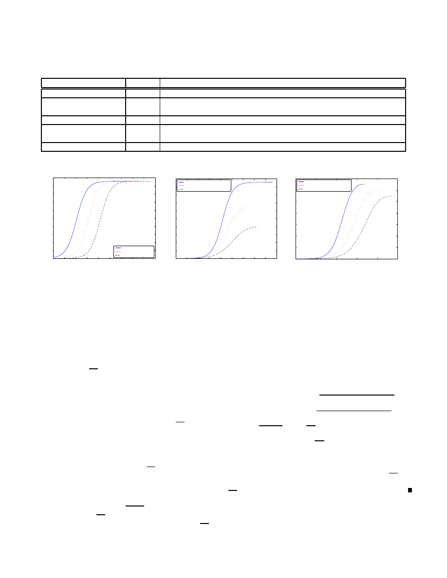
TABLE I

HE PARAMETERS FOR THE SPREAD OF ACTIVE WORMS

Parameters

Notation

Explanation

# of vulnerable machines

the number of vulnerable machines

Size of hitlist

the number of infected machines at the beginning of the spread of active
worms

Scanning rate

the average number of machines scanned by an infected machine per unit time

Death rate

the rate at which an infection is detected on a machine and eliminated
without patching

Patching rate

the rate at which an infected or vulnerable machine becomes invulnerable

100

200

300

400

500

600

700

800

900

x 10

time (second)

number of infected nodes

size of hitlist = 10000
size of hitlist = 1000
size of hitlist = 100

(a) Effect of Hitlist Size (All cases are
without patching and take a period of one
second to complete infection.)

100

200

300

400

500

600

700

800

900

x 10

time (second)

number of infected nodes

patching rate = 0 /second
patching rate = 0.0005 /second
patching rate = 0.001 /second

(b) Effect of Patching Rate (All cases have
a hitlist of 100 entries and take a period of
one second to complete infection.)

200

400

600

800

1000

x 10

time (second)

number of infected nodes

1 second to infect a machine
30 seconds to infect a machine
60 seconds to infect a machine

(c) Effect of Time to Complete Infection
(All cases have a hitlist of 100 entries and
a patching rate of 0.0005 /second.)

Fig. 1.

Modeling the Spread of Active Worms that Employ Random Scanning (All cases are for 1,000,000 vulnerable machines, a scanning rate of 100

scans/second, and a death rate of 0.001 /second.)

Although the Internet’s address space isn’t completely con-

nected, active worms always scan

entry addresses. There-

fore, for random scanning, the probability that any computer is
hit by one scan is

. Let

and

denote the total number

of vulnerable machines (including the infected ones) and the
number of infected machines at time tick

respectively.

Before the active worms spread (

#"$

and

%"$&

Theorem 1: If there are

vulnerable machines (including

the infected ones), and

infected computers, then on average,

the next time tick will have

'#)(+*-,(./,(0

/2436587

newly

infected machines, where

is the scanning rate.

ROOF

: Let

denote the number of newly infected machines

at time tick

:;<=

infected machines can generate

scans in an attempt to infect other machines. So if we can prove
that

?A@B9

EFHG

K*L,M(NO,M(

/PQ7

for any

FSR

scans, then the equation also holds when

We prove the above equation by induction on

. When

, since there are

'#T(!8

vulnerable machines that have

not yet been infected, the probability that one scan can add
a newly infected machine is

54VH365

, which is equivalent to

W(1+*-,X(Y/,Z(

. Suppose that the theorem is true

for

, i.e.,

?A@Q9

E6F

(]

K*L,^(!/,^(_

`K7

Then, when

a[cbd,

, we divide

[cb!,

scans into two parts:

the first

[

scans and the last scan. There are two possibilities

for the last scan: adding a newly infected machine or not. Let

the variable

efg,

if the last scan hits a vulnerable machine

that has not yet been infected and let

eha

otherwise. Then,

i$jKk+lLmonp>qcrtsu]vKw

xi$jKk

lLmon

p>qyrNswzu{vK|8}yx~arv|Hui$j+k

lDmon

p>qyrNsw

}yx~r]B|

xi$jKk

lLmon

p>qyrNswzu{vK|Q

l#l#i$j+kKlLm%n/p+qcrtsw

i$jKk+lLmonp>qcrtswx8vW

l#l#i$j+kKlLm%n/p+qcrtsw

ux8vz

|8i$jKk+lLmon/p>qcrtsw

|vzx8v

m%n

which means that when

Y[ZbY,

, it is also true. Therefore,

when

?A@B9

(

K*L,(AO,(

243587

That is, on the next time tick there will be

(

K*L,(/,(

/2435O7

expected newly infected machines.

Given death rate

and patching rate

, on the next time tick

there will be

infected machines that will change to

either vulnerable machines without being infected or invulner-
able machines, and the total number of vulnerable machines
(including the infected ones) will be reduced to

O,(HO#

Therefore, on the next time tick the number of total infected

machines will be

<obd({8K*L,;(!/,;(

/243

7H(

'ybNH4

. At the same time,

hO,;(o4

, which gives

I/,(So

S"$hO,(#H

. That is,

hO,M(J(ZHO>b.*DO,M(ZH

(78*L,M(NO,M(

243

(1)

where

and

. The recursion process will stop when

there are no more vulnerable machines left or when the worm
cannot increase the total number of infected machines.

Using Equation (1), we can find the characteristics of the

active worms’ spreading. For example, Figure 1(a) shows the
propagation of the active worms with different hitlist sizes.
As the size of the hitlist increases, it takes the worms less
time to spread. Figure 1(b) depicts another example. As the
patching rate grows, the spread of active worms slows down.
This complies with our intuition. It should be noted that because
the patching rate

, the two slower curves return to zero

at the end. Here, we only draw the uprising part of curves and
ignore the falling part.

At the beginning, we assume that it takes the worms one time

tick to infect a machine. To display the effect of the amount of
time it takes to infect a machine on the worm propagation, we
simply change the time unit. For example, in Figure 1(c) we
first draw the curve with a time interval of one second, which is
the amount of time required to complete infection. If the worm
needs 30 seconds to infect a machine, we set the time unit to
30 seconds, and change the corresponding

=)'

parameters

for this period of time. In this case, the parameters

=)'

will

become

====6)6+

for a time period of 30 seconds. Then,

we can use the AAWP model to get the result. But, now

expresses the number of infected machines at 30

seconds

. This figure shows the effect of the time to complete infection

on the worm’s propagation. The worm’s propagation will be
slowed down as the time required to infect a machine increases.

We can change the values of the parameters

and the time to complete infection in the AAWP model to
observe how active worms spread. This model can be used
to quantitatively explain how we can monitor the spread of
active worms, develop a sensor detection system, and evaluate
the LaBrea tool defense system, which we will cover later.

B. Comparing Our AAWP Model to the Epidemiological Model
and Weaver’s Simulator

In the Epidemiological model, a nonlinear differential equa-

tion is used to measure the virus population dynamics [7]:

!¡WO,({¢ (.6

where

W /

is the fraction of infected nodes,

is the birth rate

(the rate at which an infected machine infects other vulnerable
machines), and

is the death rate. The solution to the above

equation is

W' /W

O,;({£¤

bd/,(£Z({

V¢¥§¦V%¨©ª

(2)

where

£A

and

%"$«aW' z&=z

D¬$®¯:°Q

ª±

28ª

In fact, we can easily deduce the relationship between the

birth rate and the scanning rate:

It is interesting that when the Code Red v2 worm surged

in July of 2001, Staniford also independently presented the
same model to explain the Random Constant Spread (or RCS)
theory of the Code Red v2 worm [5]. Zou extended the Epi-
demiological model to the two-factor worm model, which takes
consideration of the human countermeasure and the worm’s
impact on Internet traffic and infrastructure [12].

The differences between the AAWP model and the Epidemi-

ological model are:

1) The Epidemiological model uses a continuous time dif-

ferential equation, while the AAWP model is based on a
discrete time model. We believe that the AAWP model is
more accurate. Because in the AAWP model, a computer
cannot infect other machines before it is infected com-
pletely. But in the Epidemiological model, a computer
begins devoting itself to infecting other machines even
though only a “small part” of it is infected. Therefore,
the speed that the worm can achieve and the number of
machines that can be infected are totally different.

2) The Epidemiological model neither considers the patch-

ing rate nor the time that it takes the worm to infect
a machine, while the AAWP model does. During the
propagation of the worm, it is possible nowadays to
promptly patch the vulnerability on computers, assuming
a reasonable patching rate. And different worms have
different infection abilities which are reflected by the
scanning rate (or the birth rate) and the time taken to
infect a machine. The time required to infect a machine
always depends on the size of the worm’ copy, the degree
of network congestion, the distance between source and
destination, and the vulnerability that the worm exploit.
From Figure 1(c), it can be seen that the time to infect
a machine is an important factor for the spread of active
worms.

3) In the AAWP model, we consider the case that the worm

can infect the same destination at the same time, while
the Epidemiological model ignores the case. In fact, it is
not uncommon for a vulnerable machine to be hit by two
(or more) scans at the same time.

Both models, however, try to get the expected number of

infected machines, given the size of the hitlist, total number
of vulnerable machines, scanning rate/birth rate and death
rate. The Epidemiological model can easily deduce the closed
form and can be used in topology orientation, such as E-mail
worms or peer-to-peer worms. In this paper, we focus on active
worms that select destinations randomly or employ local subnet
scanning, such as the Code Red and Nimda worms. Hence, the
AAWP model, which is built on the “homogeneous mixing”
topology, is sufficient for our work.

Figure 2(a) shows the comparison between these two models

with 10,000 vulnerable machines, a hitlist with 1 entry, a
birth rate of 5 /time tick and a death rate of 1 /time tick
(the parameters are from [7]). It takes the Epidemiological

1000

2000

3000

4000

5000

6000

7000

8000

time tick

number of infected nodes

AAWP model
Epidemiological model

(a) All cases are for 10,000 vulnerable machines, a hitlist with 1
entry, a scanning rate of 2147500 scans/time tick or a birth rate
of 5 /time tick and a death rate of 1 /time tick. No patching and
a time period of 1 time tick to complete infection for the AAWP
model.

100

200

300

400

500

600

x 10

time (second)

number of infected nodes

Weaver’s simulator
AAWP model
Epidemiological model

(b) All cases are for 1,000,000 vulnerable machines, a hitlist with
10,000 entries and a scanning rate of 100 scans/second. A time
period of 30 seconds to complete infection for Weaver’s simulator
and the AAWP model. A death rate of zero for both the AAWP
model and the Epidemiological model. No patching for the AAWP
model.

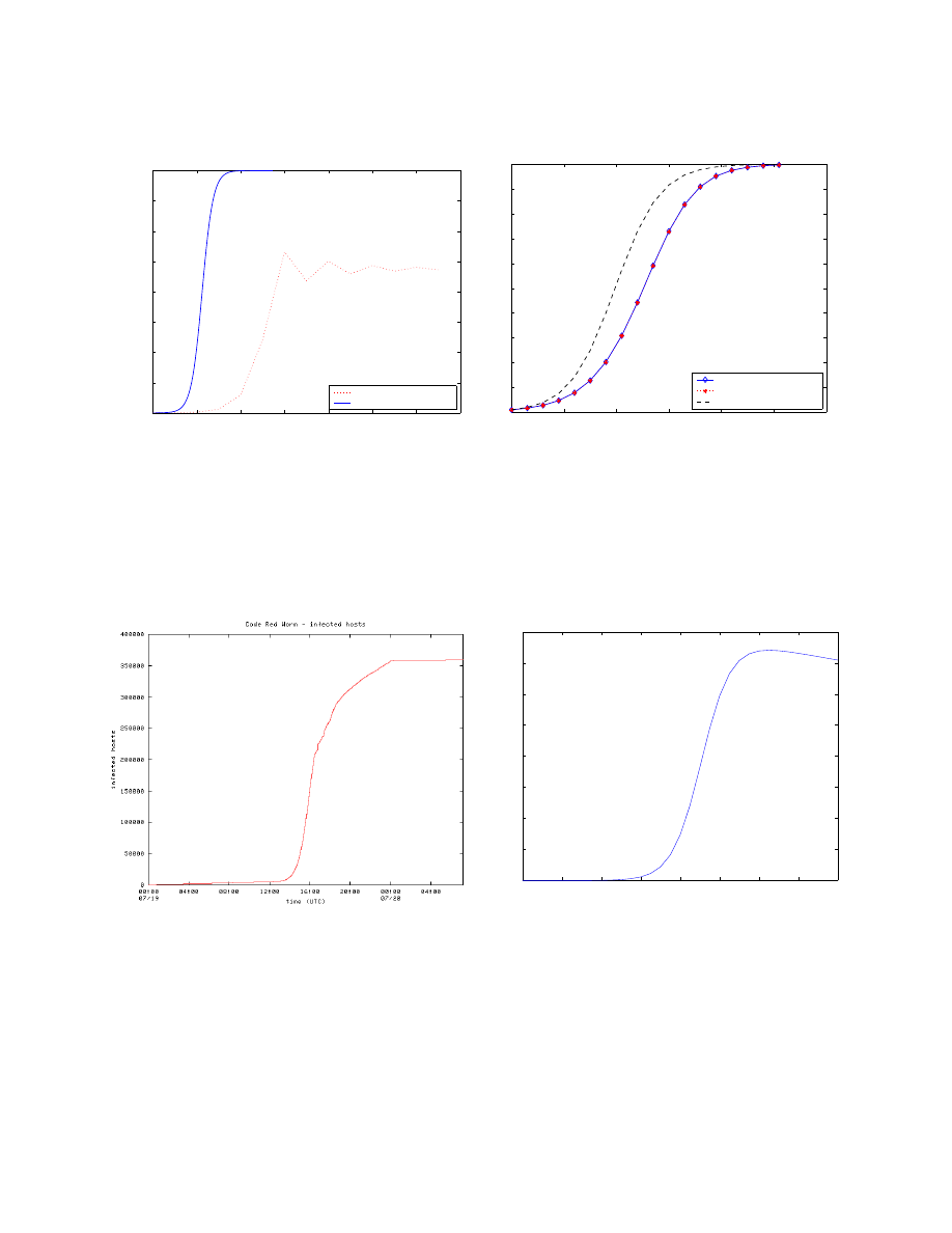
Fig. 2.

Comparing the AAWP Model to the Epidemiological model

(a) Measurement of the Code Red v2 worm spread using real data
from CAIDA.

0.5

1.5

2.5

3.5

x 10

time (hour)

number of infected nodes

(b) A simulation of the spread of the Code Red v2 worm (500,000
vulnerable machines, starting on a single machine, a scanning rate
of 2 scans/second, a death rate of 0.00002 /second, a patching rate
of 0.000002 /second, and a time period of 1 second to complete
infection).

Fig. 3.

Real Data from CAIDA [11] and Simulated Code Red v2 Like Worm from the AAWP Model

model about 4 time ticks to enter an equilibrium stage, while
the AAWP model needs about 10 time ticks. Moreover, after
entering the equilibrium stage, the Epidemiological model
totally infects 8,000 vulnerable machines (occupying

³6¤´

all vulnerable machines), while the AAWP model infects about

4,750 vulnerable machines (occupying

µ¶¤·¸=´

of all vulnerable

machines). This shows that our model can better explain the
low level of worm prevalence in [9].

Weaver wrote a small, abstract simulator of a Warhol worm’s

spread [10]. This simulator uses a 32-bit, 6-round variant

of RC5 to generate all permutations and random numbers.
We only modified one condition of this simulator to fit the
assumption which we presented above. That is, all “newly”
infected machines on a previous time tick will be activated
at the same time on the current time tick, other than based
on different clocks. Figure 2(b) shows the growing of infected
nodes with time for the two models and Weaver’s simulator,
which have the following parameters: a total of 1,000,000
vulnerable machines, a hitlist of size 10,000, a scanning rate of
100 scans/second, a death rate of zero, no patching, and a time
period of 30 seconds to infect one machine. This figure shows
that the AAWP model and Weaver’s simulator results overlap.
While our model and Weaver’s simulator take about 6 minutes
to infect

¹=´

of the vulnerable machines, the Epidemiological

model only takes about 5 minutes.

C. Simulating the Code Red v2 Worm

On July 19th, 2001, the Code Red v2 worm infected more

than 359,000 computers in less than 14 hours [11]. This worm
spreads by probing random IP addresses and infecting all
the hosts that are vulnerable to the IIS exploit. CAIDA [13]
collected real data to measure the spread of the Code Red
v2 worm. The data were collected from two locations: one /8
network at UCSD and two /16 networks at Lawrence Berkeley
Laboratory (LBL). In these data, hosts were considered to be
infected if they sent TCP SYN packets on port 80 to nonexistent
hosts on these networks. Figure 3(a) shows the number of
infected hosts over time [11].

We suppose that there are 500,000 vulnerable machines in

the Internet, the Code Red v2 worm starts on a single machine,
it performs 2 scans per second and takes one second to infect a
machine. Figure 3(b) shows the spread of the simulated Code
Red v2 like worm using our AAWP model, with a death rate
of 0.00002 /second and a patching rate of 0.000002 /second.
Because of the patching rate, the curve goes down slightly after
the worm spreads for one day.

IV. A

PPLICATIONS OF THE

AAWP

MODEL

A good model can reflect the spread of real worms and at

the same time resolve many practical task. In this section, we
apply the AAWP model to monitoring, detecting and defending
against the spread of active worms.

A. Monitoring the Spread of Active Worms

How to monitor the spreading rate of active worms is an

interesting task. It has come to our attention that CAIDA
collected real data from one /8 network at UCSD and two /16
networks at LBL [11]. Can these collected data reflect the actual
propagation of the Code Red v2 worm? Of course these data
are only the lower bound of the spread of the Code Red v2
worm. But, how much do they deviate from the reality?

Suppose that we can collect data from

KVH±$'tºY»TºI==

addresses to estimate the spread of active worms. Here, /

network is the special case of

KVH±

addresses. These addresses

0.5

1.5

2.5

3.5

x 10

time (hour)

number of infected nodes

simulated Code Red v2 like worm

addresses monitored

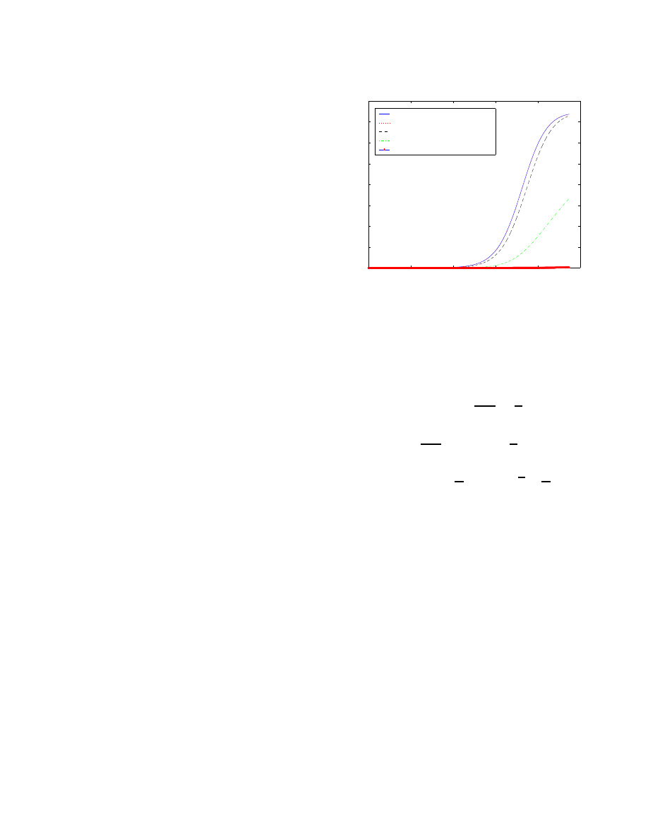
Fig. 4.

Collecting data from different address spaces. All cases were for

500,000 vulnerable machines, starting on a single machine, a scanning rate of
2 scans/second, a death rate of 0.00002 /second, a patching rate of 0.000002
/second, and a time period of 1 second to complete infection.

are considered unused IP addresses. When the scans from the
infected machine hit any address in this space, it is counted
if and only if it has not been counted before. The probability
that one scan hits this space is

1/¼=½

. If active worms

can generate

scans per time tick, then the probability that an

uncounted infected machine is observed on the next time tick
is

¾À¿ÁÂÃ,(d/,(

O¼=½

2Ä,$(YO,(

. Furthermore, if

À±

RcR

and

RcR

, then

¾À¿ÁI,(O,(

2TÅ

,({9

VJÆ

(3)

Let

Ç^

denote the number of observed infected machines

at time tick

&È=

. Before time tick

^bf,

, there are

(^Ç

uncounted infected machines. The events that uncounted

infected machines are observed are independent of one another.
Hence, the number of “newly” observed infected machines
satisfies the Binomial distribution. Then, at time tick

TbÉ,

the expected number of “newly” observed infected machines
is

¾À¿ÁÊ='

(.Ç

. Therefore,

Ç$LC

!Ç$¤bJ¾À¿Á ÊB)(Ç^8I/,(A¾À¿ÁK/Ç^bJ¾À¿Á Ê

(4)

where,

and

Ç^"a

Based on the AAWP model, we can evaluate the effect of

the different address spaces from which we collect data. Figure
4 shows one example in which we simulate the Code Red v2
worm. The curve where

/Ë

addresses are monitored is very

close to the “real” worm propagation using the AAWP model.
The curve where

addresses are monitored grows at a slower

rate than the curve where

6/Ë

addresses are monitored, but at the

same time is a much better representation than the curve where

/Ì

addresses are monitored. The curve where

addresses are

monitored gives the worst results, which can be understood
from Equation (3): when

»hµ

)¾À¿Á

, then

Ç^DC

Ç^

making the curve a horizontal line along the x-axis.

From the analysis above, we conclude that monitoring

addresses gives us a better representation of the propagation
of active worms. But an address space smaller than

is not

adequate to observe the actual spread of active worms.

B. Detection Speed

One of the goals of modeling the spread of active worms is

to be able to detect them. Here, we present a simple and useful
sensor detection system and use the AAWP model to evaluate
its performance.

1) Methodology: It is vital to detect active worms effec-

tively. In the near future active worms may spread across the
whole Internet in a very short period of time [10], making the
average detection time critical.

It is easy to figure out one simple detection system. First,

put some sensors in the Internet to monitor a set of unused
IP addresses. When the random scans from active worms hit
these IP addresses, they are detected by the sensors. However,
if the worms’ designers know which unused IP addresses mon-
itored by sensors, they could launch DoS attacks by sending
many packets to the sensors, causing them to generate many
false alarms. Therefore, sensors must have the intelligence to
distinguish between the scans from active worms and DoS at-
tacks, which requires a more complex sensor detection system.
However, this challenge is beyond the scope of this paper.

For this simple detection system, some interesting questions

need to be answered:

How many unused IP addresses should be monitored by
sensors in order to detect active worms rapidly?
Given the number of IP addresses monitored, what is the
average time required to detect worms?

2) Performance of the Sensor Detection System: The per-

formance of the sensor detection system depends mainly on
the detection time. An ideal detection system should be able to
detect active worms at the beginning of their propagation. We
use the average detection time as our performance indicator for
the sensor detection system. Let

denote the detection time.

Below, we will deduce the relationship between the average
detection time and the number of unused IP addresses that are
monitored.

Suppose that there are

unused IP addresses monitored by

sensors. For a single scan, the probability that it is detected by
sensors is

. Thus, for

scans, the probability that at least

one scan is detected by sensors is

,(O,(ÑÐ

Let

ÒA

indicate the probability that a worm is detected at

time tick

Â'ºÉAºh[ba,B

, where

Ò"f

. Also note that

at time tick

[

there are either no more vulnerable machines or

the active worms cannot increase the total number of infected
machines. Here, we assume that even if sensors fail to detect
active worms, people will finally detect them, which means

. Since

infected machines can generate

scans,

I,(O,(

2435

¼Ó

(5)

where

,ºZº<[

. Then the expected value of detection time

is:

?A@>Î

PÕ

Ê=*

PQV

±-Õ

/,;({Ò

47)Ê+Ò

(6)

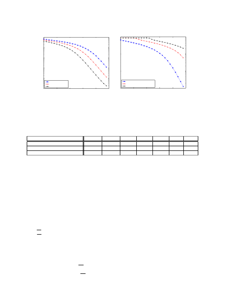
Based on the above formula and the AAWP model, Figure

5(a) shows the relationship between the average detection time
and the number of unused IP addresses that are monitored
by sensors when the active worms spread with varying hitlist
sizes. From this figure, we know that in the case of a simulated
Code Red v2 like worm (size of hitlist = 1), when monitoring

addresses, the average detection time is only about two

minutes; when monitoring

OÌ

addresses, the average detection

time increases up to about two hours. If we want to detect this
worm in one hour, more than

unused IP addresses must be

monitored by sensors. On the other hand, although the worm
with a larger hitlist spreads faster, it can also be detected in a
shorter period of time. For example, when monitoring

OÌ

addresses, we need about two hours to detect a worm starting
on a single machine, while we need 36 minutes to detect a
worm with a hitlist of 10 machines and only 5 minutes to
detect a worm with a hitlist of 100 machines. Table II shows
some sample results in Figure 5(a).

This simple detection system can be easily extended to more

complex systems. For example, to reduce the number of false
alarms, the sensors should receive several scans during a period
of one time tick before the system can actually detect worms.
Set

to be the least number of scans received by a sensor

to generate an alarm during the period of one time tick. A
larger

value generates less false alarms. The probability of

detection, however, is also reduced. Based on the definition of

, the Equation (5) becomes

I,(]ØÀÙ

±-Õ

KÚ

»OÚÛ1>

(.»1KÚ

/,(

2435

¼Ó

VH±

where

,YºÜ]ºÝ[

. Figure 5(b) shows the effect of

the sensor detection system. Even though a large

value

can reduce the number of false alarms, it reduces the overall
performance of the system. So reliability and performance
are a tradeoff. Also, if a system with a large

value does

not monitor enough addresses, it cannot completely detect the
worms. For example, when

Þ¸

and the addresses space

monitored is less than

, the system cannot detect the worms

even if the whole Internet has been infected.

C. Effectiveness of the Defense System

Another goal of modeling the spread of active worms is to

defend against active worms. Here, we extend the AAWP model
to analyze the LaBrea tool, which is put forward by Liston to
slow down or even stop the spread of active worms [14].

1) LaBrea: LaBrea is a tool that takes over unused IP ad-

dresses on a network and creates “virtual machines” that answer
to connection requests [15]. LaBrea replies to those connection
requests in such a way that causes the machine at the other end
to get “stuck”. One can intentionally hold a connection open

log

(number of unused IP addresses monitored by sensors)

expected value of detection time(second) (log)

size of hitlist = 1
size of hitlist = 10
size of hitlist = 100

(a) Effect of Hitlist Size (number of scans received = 1)

log

(number of unused IP addresses monitored by sensors)

expected value of detection time(second) (log)

number of scans received = 1
number of scans received = 2
number of scans received = 5

(b) Effect of Number of Scans Received (A hitlist with 1
entry)

Fig. 5.

Performance of sensor detection system. All cases are for 500,000 vulnerable machines, a scanning rate of 2 scans/second, a death rate of 0.00002

/second, a patching rate of 0.000002 /second, and a time period of 1 second to complete infection.

TABLE II

VERAGE

ETECTION

IME WITH

ITLISTS OF

IFFERENT

IZES AND

IFFERENT

UMBERS OF

NUSED

IP A

DDRESSES

ONITORED BY

ENSORS

ECOND

)

number of IP addresses monitored

/Ì

size of hitlist = 1

20120.00

13800.00

8241.50

4021.90

1530.60

466.28

125.00

size of hitlist =10

10007.00

5267.30

2184.70

711.70

197.14

51.14

13.25

size of hitlist =100

3030.40

1065.70

308.20

81.06

20.90

5.63

1.84

for as long as he/she wishes. That is, the LaBrea tool monitors
all traffic destined for some unused IP addresses. When one
scan hits these IP addresses (“virtual machines”), the LaBrea
tool will reply and establish a connection with the infected
machine. This connection can last for a very long time.

Before we apply the LaBrea tool extensively, we should first

attempt to answer one question: How many unused IP addresses
should be monitored by the LaBrea tool to defend against active
worms effectively?

2) Performance of the LaBrea Tool Defense System: Assume

that the LaBrea tool is installed in the Internet and is monitoring

unused IP addresses. Suppose that now there are

scans from

infected machines, beginning to search the Internet. Because the
LaBrea tool can trap the scanning threads, after one time tick,
there will be

scanning threads trapped. That is, there will

only be

O,(

scanning threads left.

Let

and

denote the average number of scans and the

number of newly infected machines at time tick

respectively. Taking into consideration that the LaBrea tool will
affect the total number of scans, we extend Equation (1) to

O,(#H

O,(.Z(#H

O,(

¢bQ9Q

K*L,(O,;(

P5Dß

O,(.Z(#H4Hb9BDC

where

and

. The recursion process

will stop when there are no more vulnerable machines left or
when the worm cannot increase the total number of infected
machines. It should be noted that if

ÏS!

, the set of formulae

outlined above turn out to be the same as Equation (1).

Figure 6 shows a simulation of a Code Red v2 like worm

spreading. When the LaBrea tool monitors less than

OÌ

unused

IP addresses, the worm spread is only slightly affected. But
when more than

unused IP addresses are monitored, the

LaBrea tool is able to effectively defend against the worm
propagation. We can also see that the total number of infected
machines stops increasing before all the vulnerable machines
are actually infected when the LaBrea monitors more than

unused IP addresses.

Therefore, the LaBrea tool can really slow down or stop

the spread of active worms. However, at least

unused IP

addresses are needed to defend against active worms effectively.
It might not be easy to persuade many network administrators
to install the LaBrea. If we can get one unused class A subnet
(an address space of

6/Ë

addresses), which is not publicly

advertised, and install the LaBrea tool to monitor the traffic into
this subnet, this seems to be a good start for fighting against
active worms.

x 10

0.5

1.5

2.5

3.5

x 10

time (second)

number of infected nodes

monitor 0 unused IP address

monitor 2

unused IP addresses

monitor 2

unused IP addresses

monitor 2

unused IP addresses

monitor 2

unused IP addresses

Fig. 6.

Performance of the LaBrea tool detection system. All cases are for

V. M

ODELING THE

PREAD OF

CTIVE

ORMS THAT

MPLOY

OCAL

UBNET

CANNING

Instead of simply selecting destinations at random, the Code

Red II and the Nimda worms preferentially search for targets
on the “local” address space [1], [3]. In this part, we extend
the AAWP to the Local AAWP (LAAWP) model to understand
the characteristics of the spread of active worms that employ
local subnet scanning.

A. LAAWP Model

As the AAWP model, the LAAWP model uses deterministic

approximation. We focus on the active worms’ scanning policy
and ignore both the death rate and the patching rate to simplify
the model. The function of firewalls is not considered, either.

Now suppose that a worm scans the Internet as follows:

of the time, a random address will be chosen

of the time, an address with the same first octet will

be chosen

of the time, an address with the same first two octets

will be chosen

where,

"b$

. We can regard random scanning as one

special case of local subnet scanning, when

"Þ,

and

Assume that the vulnerable machines are evenly distributed

in every subnet which is identified by the first two octets. The
subnets can be classified into three different kinds of networks:

A “special” subnet (denoted by Subnet type 1), which
always has a larger hitlist size.

6Í (,

subnets having the same first octet as the “special”

subnet (denoted by Subnet type 2).
Other

/Ì

(]Í

subnets (denoted by Subnet type 3).

Different kinds of networks have hitlists of different sizes. In
the same type of subnet, all networks have the same hitlist size.

Let

, and

denote the size of the hitlist in Subnet type

1, 2, and 3, respectively.

Let

, and

denote the average number of infected

machines in Subnet type 1, 2, and 3, respectively. And let

, and

denote the average number of scans hitting

Subnet type 1, 2, and 3, respectively. Then at some time tick,
the relationship between the average number of scans hitting
Subnet type

#'à,6¿B¾á

and the average number of

infected machines in different Subnets is

BÁ

b&1

(,BMÊQÁ

(,QMÊBÁ

b&1

/Ì

(]

zÊQÁ

OÌ

BÁ

b&1

(,BMÊQÁ

(,QMÊBÁ

b&1

/Ì

(]

zÊQÁ

OÌ

BÁ

QÁ

)"Q*

(,QMÊBÁ

b&1

/Ì

(]

zÊQÁ

OÌ

For

(

cÃ,=X¿B¾

), the first item is the average number

of scans coming from the local subnet (with the same first two
octets). The second item is the average number of scans coming
from neighboring subnets (with the same first octet). And the
last item is the average number of scans coming from global
subnets.

In every subnet the scans will randomly hit targets, which

can be modeled by the AAWP model. The total number of
machines will be

/Ì

, instead of

, and the total number of

scans will be

. Thus, Equation (1) becomes

Áâ

&Á

bgã

/Ì

(]Á

äÉå

,(æã%,(

OÌ

5ç

(7)

where,

,6M¿B¾$

and

is the number of infected machines

on the next time tick. The recursion process will stop when
there are no more vulnerable machines left. At some time tick,
the total number of infected machines will be

bdÍ$(a,QzÊ

b&1

OÌ

(]ÍQMÊQÁ

Based on the above formulae, we can understand the charac-

teristics of local subnet scanning and the effect of the hitlist’s
distribution. Different

)"6M

and

;

can generate

different patterns for the spread of worms.

Four cases are considered here:

1) Random scanning (

"è,

): In this

case

Uë

4ìy®¯

ª'í±

¯Q/î

î4°>

Ó'ï

which means the distribution of the hitlist cannot effect
the spread of active worms.

2) A hitlist with an even distribution (

): This

gives

\BÁ

gQÁ

gBÁ

. Local subnet

scanning, therefore, cannot change the spread of active
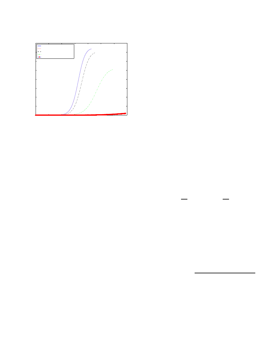
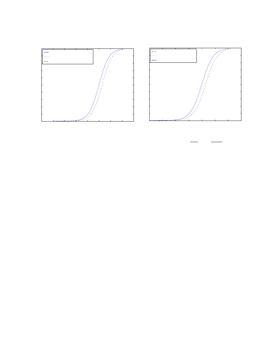
worms in this case.

3) Similar to the Nimda worm (

à·6¸

ð·

=¸

ñ·¸

): In this case, we select different distributions

of the hitlist, just as in Figure 7(a). Evenly distributed
hitlists give the best performance, while putting all hitlists
together in one “special” subnet (

I,QW

)

gives us the worst performance. This figure shows that

100

200

300

400

500

600

700

800

x 10

time tick

number of infected nodes

=10/2

, h

=10/2

, h

=10/2

, h

=10/2

, h

=10, h

=0, h

(a) Local subnet scanning with different hitlist distributions. All
cases are for

òózô#õQö

÷øQùò

ôõQö

÷øQùò

ôõQö

100

200

300

400

500

600

700

x 10

time tick

number of infected nodes

= 0, p

= 1

= 0.25, p

= 0.5

= 1, p

= 0, p

= 0

(b) Local subnet scanning with an uneven hitlist distribution. All
cases are for

ôNû/õQù¢ú

ôýü

8þ+ÿ

ù¢ú

Ó'ï

ÿ8þ

Fig. 7. Modeling the Spread of Active Worms that Employ Local Subnet Scanning (All cases are for 1,000,000 vulnerable machines which are evenly distributed
to every subnet, a scanning rate of 100 scans/time tick and a time period of 1 time tick to complete infection.)

the hitlist’s distribution can affect the spread of active
worms.

4) Local subnet scanning with a hitlist of uneven distribution

(fix

and let

): This stands for a

hitlist of uneven distribution and a centralization of more
hitlist machines in the “special” subnet. Surprisingly,
however, Figure 7(b) shows that in this case local subnet
scanning slows down the propagation of active worms.
We will further discuss why worm designers select this
scanning technique in the next section.

From the four cases above, we see that for local subnet

scanning the hitlist’s distribution can influence the spread of
active worms, while the even distribution gives us the best
performance. In addition when the hitlist is more concentrated
in the “special” subnet, local subnet scanning slows down the
spread of active worms.

B. Discussion of the Local Subnet Scanning Policy

The LAAWP model implies that local subnet scanning may

slow down the spread of active worms. Why do the designers of
active worms use this technique? There are two main reasons:

1) Firewalls can protect vulnerable machines behind it. But

local subnet scanning allows a single copy of a worm
running behind the firewall to rapidly infect all the other
local vulnerable machines.

2) One subnet always belongs to a company or organization

and has a lot of similar machines. Therefore, it can be
expected that if a machine has a security hole, then there
is a high probability that many other machines in the
same network have the same security hole.

VI. C

ONCLUSIONS

In this paper we present the AAWP model to analyze the

characteristics of the spread of active worms. Even though the
AAWP model also used deterministic approximation, it gives
more realistic results when compared to the Epidemiological
model. The simulation results show that our model can better
explain the “mystery” in [9]. The AAWP model can be used to
simulate the Code Red v2 worm with the following parameters:
500,000 vulnerable machines, starting on a single machine,
a scanning rate of 2 scans/second, a death rate of 0.00002
/second, a patching rate of 0.000002 /second, and a time period
of 1 second to complete infection.

Taking the Code Red v2 worm as an example, we apply

our model to answer three different questions. First, from our
model we assert that an address space of

/Ë

IP addresses is

large enough to obtain realistic results, while an address space
smaller than

addresses is not large enough to effectively

obtain any realistic information about the spread of worms.
Second, the AAWP model is used to evaluate the performance
of a simple sensor detection system. More than

unused IP

addresses are needed for the sensors to detect the Code Red
v2 like worm in one hour. Worms with a larger hitlist can be
detected in a shorter period of time, even though they spread
at a much faster rate. This simple sensor detection system is
the first step towards a practical detection system that detects
active worms through scanning frequencies or source IP address
distributions. We plan to use our model to evaluate this type of
detection system. Finally, the AAWP model is used to evaluate
the performance of the LaBrea tool defense system. Similarly,
an address space of more than

unused IP addresses is

needed by LaBrea to defend against the Code Red v2 like worm

effectively. We plan to apply our model to assess other publicly
available defense systems and compare the relative performance
of different defense systems.

As part of our ongoing work, we extend the AAWP model

to the LAAWP model to understand the spread of active worms
using local subnet scanning. The distribution of the hitlist can
affect the local subnet scanning policy. In particular, a worm
using an evenly distributed hitlist spreads at the fastest rate.
When the hitlist is concentrated in some subnet, the spread
of active worms is slowed down. In the LAAWP model, the
vulnerable machines are assumed to be evenly distributed in
every subnet. We plan to study the effect of the distribution of
vulnerable machines in order to get more accurate results.

EFERENCES

[1] R. Russell and A. Machie, “Code Red II Worm,” Incident Analysis,

SecurityFocus, Tech. Rep., Aug. 2001.

[2] A. Machie, J. Roculan, R. Russell, and M. V. Velzen, “Nimda Worm

Analysis,” Incident Analysis, SecurityFocus, Tech. Rep., Sept. 2001.

[3] CERT/CC,

“CERT

Advisory

CA-2001-26

Nimda

Worm,”

http://www.cert.org/advisories/CA-2001-26.html, Sept. 2001.

[4] D.

Song,

Malan,

and

Stone,

“A

Snap-

shot

Global

Internet

Worm

Activity,”

http://research.arbornetworks.com/up media/up files/snapshot worm activity.pdf,
Arbor Networks, Tech. Rep., Nov. 2001.

[5] S. Staniford, V. Paxson, and N. Weaver, “How to 0wn the Internet in Your

Spare Time,” in Proc. of the 11th USENIX Security Symposium (Security
’02), 2002.

[6] J. O. Kephart and S. R. White, “Measuring and modeling computer virus

prevalence,” in Proc. of the 1993 IEEE Computer Society Symposium on
Research in Security and Privacy, May 1993, pp. 2–15.

[7] J. O. Kephart, “How topology affects population dynamics,” in C.

Langton, ed., Artificial Life III. Studies in the Sciences of Complexity,
1994, pp. 447–463.

[8] J. O. Kephart and S. R. White, “Directed-graph Epidemiological Models

of Computer Viruses,” in Proc. of the 1991 IEEE Computer Society
Symposium on Research in Security and Privacy, May 1991, pp. 343–359.

[9] S. R. White, “Open Problems in Computer Virus Research,” Oct. 1998,

presented at Virus Bulletin Conference.

[10] N. Weaver, “Warhol Worms: The Potential for Very Fast Internet Plagues,”

http://www.cs.berkeley.edu/

nweaver/warhol.html.

[11] D.

Moore,

“The

Spread

the

Code-Red

Worm

(CRv2),”

http://www.caida.org/analysis/security/code-red/coderedv2 analysis.xml.

[12] C. C. Zou, W. Gong, and D. Towsley, “Code Red Worm Propagation

Modeling and Analysis,” in 9th ACM Conference on Computer and
Communication Security, Nov 2002.

[13] CAIDA,

“CAIDA

Analysis

Code-Red,”

http://www.caida.org/analysis/security/code-red/.

[14] T. Liston, “Welcome To My Tarpit - The Tactical and Strategic Use of

LaBrea,” http://www.hackbusters.net/LaBrea/LaBrea.txt.

[15] ——, “LaBrea,” http://www.hackbusters.net/LaBrea/.

Wyszukiwarka

Podobne podstrony:
Why Anti Virus Software Cannot Stop the Spread of Email Worms
A Filter That Prevents the Spread of Mail Attachment Type Trojan Horse Computer Worms
8 0 1 2?tivity Modeling the Internet of Everything (IoE)
On the Spread of Viruses on the Internet
Modeling the Effects of Timing Parameters on Virus Propagation
Email networks and the spread of computer viruses
The Future of Internet Worms
Frederik Kortlandt The Spread Of The Indo Europeans
Suppressing the spread of email malcode using short term message recall
The Invention Of Active Flag And Loop Antennas
Far Infrared Energy Distributions of Active Galaxies in the Local Universe and Beyond From ISO to H
Woziwoda, Beata; Kopeć, Dominik Changes in the silver fir forest vegetation 50 years after cessatio
On the trade off between speed and resiliency of Flash worms and similar malcodes
Adsorption of active ingredients of surface disinfectants depends on the type
Multiscale Modeling and Simulation of Worm Effects on the Internet Routing Infrastructure
The Evolution of Viruses and Worms
The Impact of Countermeasure Spreading on the Prevalence of Computer Viruses
On the Infeasibility of Modeling Polymorphic Shellcode for Signature Detection

więcej podobnych podstron