
This page intentionally left blank

The Politics of Income Inequality in the United States
This book revolves around one central question: Do political dynamics
have a systematic and predictable influence on distributional outcomes
in the United States? The answer is a resounding yes. Utilizing data
from mass income surveys, elite surveys, and aggregate time series, as
well as theoretical insights from both American and comparative pol-
itics, Kelly shows that income inequality is a fundamental part of the
U.S. macro political system. Shifts in public opinion, party control of
government, and the ideological direction of policy all have important
consequences for distributional outcomes. Specifically, shifts to the left
produce reductions in inequality through two mechanisms – explicit
redistribution and market conditioning. Whereas many previous stud-
ies focus only on the distributional impact of redistribution, this book
shows that such a narrow strategy is misguided. In fact, market mech-
anisms matter far more than traditional redistribution in translating
macro political shifts into distributional outcomes.
Nathan J. Kelly is Assistant Professor of Political Science at the Uni-
versity of Tennessee. He received an M.A. and Ph.D. in political
science from the University of North Carolina at Chapel Hill and a
B.A. from Wheaton College (IL). He is the winner of the Raymond
Dawson Fellowship and the James Prothro Award from the University
of North Carolina Department of Political Science and was named a
finalist for the E. E. Schattschneider Award for the best dissertation in
American politics, awarded by the American Political Science Associ-
ation. His research, supported in part by a grant from the National
Science Foundation, has appeared in various journals, including the
American Journal of Political Science and Political Analysis.

To Bud Kellstedt, for showing me how exciting the research
enterprise can be
and
To Jana, for never letting me forget that inequality exists, and
that it matters

The Politics of Income Inequality
in the United States
NATHAN J. KELLY
University of Tennessee

CAMBRIDGE UNIVERSITY PRESS
Cambridge, New York, Melbourne, Madrid, Cape Town, Singapore, São Paulo
Cambridge University Press
The Edinburgh Building, Cambridge CB2 8RU, UK
First published in print format
ISBN-13 978-0-521-51458-3
ISBN-13 978-0-511-50848-6
© Nathan J. Kelly 2009
2009
Information on this title: www.cambridge.org/9780521514583
This publication is in copyright. Subject to statutory exception and to the
provision of relevant collective licensing agreements, no reproduction of any part
may take place without the written permission of Cambridge University Press.
Cambridge University Press has no responsibility for the persistence or accuracy
of urls for external or third-party internet websites referred to in this publication,
and does not guarantee that any content on such websites is, or will remain,
accurate or appropriate.
Published in the United States of America by Cambridge University Press, New York
eBook (NetLibrary)
hardback

Contents
List of Figures
page
List of Tables
Acknowledgments
1
Explaining Income Inequality
Equality and Inequality in the World’s Richest Country
Trends in U.S. Income Inequality
Theoretical Foundations: Political Dynamics and
Distributional Outcomes
An Outline of the Book
2
The Distributional Force of Government
Mechanisms of Distributional Impact
Conclusion
3
Political Conflict over “Who Gets What?”
A Case Study in Distributional Debate: The Marriage
Tax “Penalty”
Systematic Evidence of the Partisan and Ideological
Divide over Distributional Outcomes
Conclusion
4
Party Dynamics and Income Inequality
A Theory of Distribution and Redistribution in
the United States
v

vi
Contents
Assessing the Effect of Market and Political Power
Resources on Distributional Outcomes
Conclusion
5
Macro Policy and Distributional Processes
Micro and Macro: The Logic of Macro Politics
Macro Politics, Power Resources, and the Distributional
Consequences of Policy
Conceptualizing and Measuring Macro Policy:
Micro vs. Macro
Policy and Distributional Outcomes, 1947–2000
Conclusion
6
Putting the Pieces Together: Who Gets What
and How
A More Complete Picture of Politics and Income
Inequality
The Comprehensive Model: A Simultaneous Equation
Approach
Does Politics Really Matter?
Conclusion
7
Distribution, Redistribution, and the Future of
American Politics
How Does Politics Influence Who Gets What?
American Inequality in the Twenty-First Century:
Looking Forward
Appendix A: Congressional Questionnaire
Appendix B: Measuring Income Inequality
over Time
Bibliography
Index

Figures
1.1 Share of Household Money Income Held by
Each Quintile in the United States, 2000
page 5
1.2 Income Inequality in Nine Countries
8
1.3 Gini Coefficient: 1913–2000
10
1.4 Income Share of Top 5 Percent: 1913–2000
11
1.5 Changes in Income Share by Income Quintile:
1973–2000
11
1.6 The Macro Politics Model and Distributional
Outcomes
14
1.7 The Traditional Power Resources Model of
Distributional Outcomes
15
1.8 The Overarching Model: Combining Macro
Politics and Power Resources
16
2.1 Income Distribution by Quintile for
Pre-Redistribution Income
26
2.2 Reduction in Inequality Attributable to
Federal Tax Programs in the United States
30
2.3 Share of Social Security and Medicare Benefits
Received by Each Income Quintile
32
2.4 Reduction in Inequality Attributed to Social
Security and Medicare Benefits
33
2.5 Equalizing Effect of Non-Means-Tested
Government Benefit Programs
35
vii

viii
List of Figures
2.6 Equalizing Effect of Means-Tested
Government Benefit Programs
36
2.7 Combined Equalizing Effect of Government
Action in the United States
39
4.1 Pre-Redistribution Inequality: 1947–2000
95
4.2 Redistribution: 1947–2000
96
4.3 Post-Government Inequality: 1947–2000
96
4.4 Power Resources Portion of the Model
102
5.1 Policy and Two Mechanisms of Distributional
Impact
126
5.2 Policy Liberalism (Detrended), 1947–2000
129
6.1 A Depiction of the Models Examined in
Chapters 4 and 5
137
6.2 A Path Model of Macro Politics, Power
Resources, and Distributional Outcomes
143
6.3 Path Diagram for Full Model, Standardized
Short- and Long-Term Impact
151
6.4 Actual and Simulated Post-Government Inequality
without LBJ and 1965 Great Society Programs
160

Tables
1.1 Aggregate Economic Indicators in the United
States, 2000
page 3
1.2 Consumer Expenditures in the United States, 2000
4
1.3 Income at Selected Positions in the Income
Distribution, 2000
6
2.1 Distribution of Federal Taxes and Earned
Income Credit, 2000
29
2.2 Distribution and Level of Income by Deciles
in the United States, 2000
37
3.1 Marriage Bias in the Federal Income Tax
53
3.2 Tax Cuts (in $billions) to Married Couples at
Specified Levels of Taxable Income
60
3.3 Comparison of Respondents and Full House
Characteristics
69
3.4 Partisan Differences in the House Regarding
Preferred Salary Levels
71
3.5 Partisan Differences in the House Regarding Seven
Economic Outcomes
73
3.6 Partisan Differences in the House Regarding
Distributional Preferences and State Intervention
to Increase Equality
75
3.7 Partisan Differences in the House Regarding
Government Provision of Benefits
77
ix

x
List of Tables
4.1 Change in Pre-Redistribution Inequality by
Presidential Administration, 1948–2000
99
4.2 Change in Redistribution by Presidential
Administration, 1948–2000
100
4.3 Explaining Government Redistribution,
1947–2000
107
4.4 Explaining Pre-Redistribution Inequality,
1947–2000
112
5.1 Public Policy and Government Redistribution,
1947–2000
131
5.2 Public Policy and Pre-Redistribution Inequality,
1947–2000
133
6.1 Estimating a Structural Model of Distributional
Outcomes
148
6.2 Total Effects (standardized) of Power Resources,
Macro Politics, Demographics, and Labor
Market on Distributional Outcomes
153
B.1 Distribution of Money Income for Families,
Unrelated Individuals, and Households: 1967
179
B.2 A Method for Computing Income Distribution
over Time Illustrated with Data from 2000
180

Acknowledgments
It is trite, but certainly true, that authors accrue several debts of
gratitude in the course of any project. I am no exception. The ini-
tial idea for this book sprang from a conversation with Jim Stimson
during graduate school. Jim’s contributions to this effort did not stop
with that initial conversation. For many months, he worked tirelessly
to help me refine ideas and develop the skills necessary to test them.
Along the way, the early stages of this research agenda led to a disser-
tation, which Jim directed. Simply stated, this project would not have
come to fruition without the help and support of Jim Stimson.
I also appreciate the help that the other members of my dissertation
committee – David Lowery, Mike MacKuen, George Rabinowitz, and
John Stephens – provided in moving this project from a dissertation to
a book. David Lowery was particularly helpful in pointing me in some
useful directions at the beginning of the project, and John Stephens
was the first to suggest that I explore how comparative theories might
enhance my work.
During the course of this project, several people have read and
commented on aspects of the research program. I thank the following
people for their generosity and thoughtful consideration of my work:
Michelle Benson, Johanna Birnir, David Brule, Ian Down, Sean Erlich,
Chuck Finocchiaro, Richard Fording, David Houston, Mark Hurwitz,
Wonjae Hwang, Gregg Johnson, Christine Kelleher, Paul Kellstedt,
Jens Ludwig, Andrea McAtee, Jana Morgan, Tony Nownes, Mark
Rom, Matt Schneider, Paul Senese, Terry Sullivan, Chris Wlezien,
xi

xii
Acknowledgments
Jennifer Wolak, the political science departments at the University at
Buffalo and Tufts University, and participants in the Duke-UNC Amer-
ican Politics Research Group. I am also grateful to Chris Reinard and
James Trimble for their research assistance and to Marcus Friesen for
his invaluable help during my time in Washington, DC.
The political science departments at the University of Tennessee,
the University at Buffalo, and the University of North Carolina sup-
ported this project though travel funding, administrative support, and
release-time from teaching. Grants and awards funding this project
came from the following organizations: the Duke-UNC American
Politics Research Group, the Chancellor’s Office at the University
of Tennessee, and the National Science Foundation (Grant Number
SES-0318044). Any opinions, findings, and conclusions or recommen-
dations expressed in the material are, of course, mine and do not
necessarily reflect the views of any of the funding organizations.
Eric Crahan has been a joy to work with. I thank him for his
support of this project and his professionalism throughout the pro-
cess. Also, every member of the staff at Cambridge has worked
to make the publication process as smooth as possible. Small por-
tions of Chapters 4 and 5 of this book are reprinted from an earlier
article (Kelly 2005). I thank Blackwell Publishing and the Midwest
Political Science Association for granting permission to reprint this
material here.
The work to produce this book took many years, and there were
numerous individuals in my life during this time who provided me
with various forms of support and encouragement. I owe special
thanks to the following dear friends: Doug Banister, Ashlea Cata-
lana, Michael Catalana, Lynn Charles, Kathy Evans, Turner Howard,
Jeremy Jennings, Mary Jennings, Breese Johnson, David Johnson, Peter
Johnson, Travetta Johnson, Heather Kane, Patrick King, Judy Long,
Kevin O’Donovan, Laurens Tullock, Polly Tullock, Ashley Walker,
and Russ Walker. My parents, Connie Kelly and Milt Kelly, as well as
my in-laws, Kathy Morgan and Harry Morgan, have been extraordi-
narily supportive. I also thank my brothers, Jon Kelly and Ben Kelly, as
well as my siblings-in-law, Alyssa Lovell and Matt Lovell, for always
pushing me to be my best.
Finally, I owe the largest debt of gratitude to Jana Morgan. Her
support of this project has been both professional and personal. I

Acknowledgments
xiii
first thank Jana for commenting on every component of this research
program from start to finish. In fact, the earlier reference to John
Stephens’s help on this project would not have happened had Jana not
pressed me to seek John as an addition to my dissertation committee.
She has continually pushed my thinking in new and better directions.
Jana also poured over every page of this manuscript. Her eye for detail
prevented several errors, and, I am sure, made this book better in innu-
merable ways. Remaining errors, however, are mine alone. Jana is the
best professional colleague that I could have asked for on this project.
Her support goes well beyond the professional. People ask me all
the time what it is like to have a spouse who shares my profession.
The premise always seems to be that it must be very hard. While it is
true that our professional lives can pervade almost everything we do,
my response to this common query is always the same – “It’s great!” I
consider myself one of the most fortunate people in the world to have
a spouse who not only understands me but understands my work as
well. Throughout this project, Jana always provided the sort of spousal
encouragement that is typically acknowledged by authors. She prodded
during times of discouragement or lack of energy. She provided reality
checks when I (rarely) thought things were perfect. She gave me the
freedom to do what I needed to do to see this project to completion.
But on top of all this, Jana understands theory development, research
design, and quantitative analysis. I am not sure what more I could ask!


1
Explaining Income Inequality
“Who gets what?” is arguably the most important question of politi-
cal contestation. The answer to this question determines equality and
inequality in society. Of course there are many forms of inequality.
Political inequality, racial inequality, social inequality, power inequal-
ity, and economic inequality, to name a few, have received attention
from journalists, pundits, and social commentators, as well as schol-
ars from a variety of academic disciplines (Danziger and Gottschalk
1995, Harris et al. 2004, Johnston 2007, Keister 2000, McCarty
et al. 2006, Page and Simmons 2000). While various forms of inequal-
ity are almost certainly interconnected, this book explicitly examines
one specific form of inequality – economic inequality.
I focus on income distribution as a primary indicator of economic
inequality.
1
The amount of inequality present in the income distribu-
tion presents an empirical answer to the question of “Who gets what?”
I assess the (national) government role, the actions and policies by
which government balances – or unbalances – the scales of equality.
1
The other primary indicator of economic inequality that I considered analyzing is
wealth inequality. I elected to focus on income inequality for three primary reasons.
First, income is an important determinant of the material goods that people can obtain
in the short term while wealth is a better indicator of long-term economic well-being,
and politics more commonly focuses on the short term. Second, high-quality data on
incomes in the United States are readily available over a long time-span, but wealth
data are only available more recently and the data are of much lower quality. Finally,
income inequality is the most commonly discussed distributional outcome in recent
studies of U.S. politics.
1

2
The Politics of Income Inequality in the United States
Much of the story of equality and inequality must be a tale of changes
in a market economy. But an important and often neglected part of
the story concerns government and how policies benefit some people
at the expense of others. That is my focus.
When Richard Nixon took the oath of office in 1969, he inher-
ited an economy in which American incomes were more equal than
when his predecessor took office, more equal in fact than ever before.
While the most reliable data on income inequality go back only to the
late 1940s, evidence pieced together by economic historians indicates
that after a spike in inequality precipitated by the Great Depression,
inequality declined steadily for several decades. Every four-year period
brought a new level of equality to American society. It was never to
be again. Following the Nixon/Ford presidencies, every new president
took control of an economy that was less equal than it had been four
years before. How could America trend toward equality for most of
the twentieth century and then reverse course?
equality and inequality in the world’s
richest country
Despite some recent and dramatic difficulties, there is no doubt that
citizens of the United States participate in one of the most prosperous
economies in the world. I begin exploring income inequality by pro-
viding a detailed look at who has the money in the United States. The
goal is to paint a basic picture of economic conditions in the United
States and describe how the economic pie is divided.
Economic Prosperity in the United States
How prosperous is the United States? There are several approaches to
answering this question. One of them is to compare the United States
to other countries around the globe. In Table 1.1, I report the U.S.
ranking among OECD countries for several economic indicators. One
of the most basic gauges of a country’s aggregate prosperity is the total
value of goods and services it produces within its borders. By this most
rudimentary measure, in the year 2000 the United States was the largest
economy in the world. With a GDP of nearly $10 trillion, the United

Explaining Income Inequality
3
table 1.1. Aggregate Economic Indicators in the United
States, 2000
Indicator
OECD Rank out of
30
GDP
1 ($9,764 billion)
GDP Growth
6 (6%)
GDP Per Capita (Exchange Rate Method)
4 ($34,575)
Unemployment
5 (4%)
Inflation
9 (2%)
Source: OECD and World Bank.
States’ nearest competitor was Japan, with an economy approximately
half as large.
The overall size of an economy, however, could be only marginally
related to the prosperity of its individual members. China, for exam-
ple, has a large GDP, but its population is also large. But the United
States is also near the top of the heap in GDP per capita and, in addi-
tion, has comparatively low rates of inflation and unemployment. In
2000, money and jobs were plentiful and prices were relatively stable.
Though the situation has ebbed somewhat in the intervening period,
this has been a common description of economic conditions for much
of America’s recent past.
If we look underneath these highly aggregated numbers, we find
that the average American family at the end of the twentieth century
clearly enjoyed the material fruits of a strong aggregate economy (see
Table 1.2). The median price of a new home was $169,000, Amer-
icans owned 2.1 automobiles per household, and they spent more
than $4000 annually per household on hotels and restaurants. With
a median household income of more than $40,000 per year, the aver-
age American household was able to partake of a variety of goods
and services that residents of many other countries would consider
luxuries. When American households spend more than $100 per year
on audio compact disks and more than $700 on alcoholic beverages,
it would be hard to argue that the American macro economy is in
crisis. While the U.S. economy goes through its ups and downs, Amer-
icans generally remain an economically privileged group. The United
States undoubtedly has one of the most prosperous economies in the
world.

4
The Politics of Income Inequality in the United States
table 1.2. Consumer Expenditures in the United States, 2000
Measure
Value
Median Household Income
$41,578
Median Price of New Home
$169,000
% Households with Personal Computer
51%
% Households with Internet Connection
44%
Wireless Phone Subscribers Per Household
0.97
Telephone Lines Per Household
1.79
Automobiles per Household
2.1
Alcoholic Beverages Expenditures Per Household
$711
Tobacco Expenditures Per Household
$677
Hotel and Restaurant Expenditures Per Household
$4138
Compact Disk Expenditures Per Household
$129
Sources: U.S. Census Bureau; Euromonitor (2002).
Big and Small Slices of a Large Economic Pie
The economic pie in the United States is large, but the way it is divided is
also important. When we start to talk about politics – who gets what –
we are inherently focusing on areas of conflict, and politics is what this
book is about. An examination of who gets what in a society points us
toward indicators of relative rather than absolute prosperity. Income
inequality is a key indicator of relative prosperity, and it is my focus.
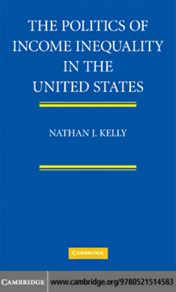
Figure 1.1 presents a rudimentary picture of how economic pros-
perity is divvied up in the United States.
2
In this figure, I report the
2
The data here and in the rest of the book come from the March Supplement to the
Current Population Study (CPS) conducted by the United States Census Bureau. The
CPS is a monthly survey of American households. Each month, approximately 50,000
households are sampled for participation in the CPS, and respondents are interviewed
in order to obtain information about the employment status, earnings, hours of work,
demographics, and educational attainment of all members of the sampled household
over the age of 15. While this monthly survey collects information about wages earned
by the various members of the household, it does not provide any more detailed
information about the income earned within the household. However, on an annual
basis, the CPS asks more detailed questions about income and work experience from
the previous year in the Annual Demographic Survey, or March Supplement to the
CPS. Beginning in 2003, the Annual Demographic Survey is called the Annual Social
and Economic Supplement (ASES).
As far back as 1947, the CPS (it was the April survey in that time) asked respondents
about the income from a handful of general sources earned during the previous year
by members of the household. In the most recent data, information about income
from over 50 separate sources including earnings, wages, tips, and government cash
Explaining Income Inequality
5
4%
9%
15%
23%
49%
0
5
10
15
20
25
30
35
40
45
50
Percent of aggregate
income
1
Income quintile (lowest to highest)
2
3
4
5
figure 1.1. Share of Household Money Income Held by Each Quintile in the
United States, 2000
share of aggregate money income held by each income quintile, from
poorest to richest.
3
Later in the book I expand the examination beyond
the basic money income definition that is the standard reported by the
U.S. Census Bureau. This is a good place to start, though, because
when the news reports that “median household income rose by 2.3
percent between 1986 and 1987,” it refers to money income.
4
What Figure 1.1 makes crystal clear is that the blessings of economic
prosperity in the United States do not fall equally on everyone. Some
benefits is solicited. This makes the March CPS the most comprehensive, consistently
available source of household income data in the United States.
3
The household is the unit of analysis utilized throughout this book. One could also
examine income inequality across families, or individuals, or even counties for that
matter. The decision regarding unit of analysis is not trivial, and households are gen-
erally viewed as the most appropriate and inclusive unit of analysis. Analyzing only
families, for example, excludes unrelated people living together in a housing unit.
Examining individuals raises obvious problems about the inclusion or exclusion of
children. Households include families and unrelated individuals and create fairly com-
parable units of analysis, though important differences across households will always
exist.
4
Money income can be thought of as income that comes or could come in the form
of a direct cash payment. Specifically, money income includes the following sources:
earnings from an employer, unemployment compensation, workers’ compensation,
Social Security, Supplemental Security Income, public assistance, veterans’ payments,
survivor benefits, disability benefits, pension or retirement income, interest, dividends,
rents, royalties, estates, trusts, educational assistance, alimony, child support, financial
assistance from outside the household, and other money income.

6
The Politics of Income Inequality in the United States
have a lot, while others have relatively little. Keep in mind that each
income quintile represents exactly the same number of households.
The top income quintile, however, received vastly more income than
the households in the bottom quintile. In fact, the top 20 percent of
households received about 3.25 times as much income as the bottom
40 percent combined, and the richest quintile was, in fact, more than
12 times richer than the poorest quintile of households.
A second way to view the division of the economic pie in the
United States is to examine the household income levels at different
positions in the income distribution. To make the concept of income
inequality more readily grasped, I report the amount of money income
received by households at specified points in the income distribution
(see Table 1.3). How much income does the household at the 10th
percentile (the household richer than 10 percent of other households)
make compared to the household at the 95th percentile?
While it may be hard to understand the meaning of the fact that
the bottom income quintile receives 4 percent of aggregate income,
it should be easy to comprehend that the household at the 10th per-
centile of the U.S. income distribution earns an income of $10,991.
table 1.3. Income at Selected Positions in the Income Distribution,
2000
Percentile
Income
Example Occupations
10th
$10,991
Food Preparation; Teachers’ Aide
20th
$18,000
Nursery Worker; Dental Assistant; Security Guard;
Bank Teller
30th
$25,030
Food Service Supervisor; Truck Driver; Machine
Operators
40th
$32,763
Auto Mechanic; Dental Hygienist
50th
$41,990
Plumber; Technical Writer
60th
$51,565
Architect; Elementary Teacher
70th
$64,002
Financial Manager; Sales-Financial Services
80th
$80,288
Full Professor (Doctoral); Attorney
90th
$109,264
Advertising Executive
95th
$143,500
Family Practice Physician
Note: Listed example occupations approximate average annual income for full and
part-time employees at the specified percentile.
Sources: U.S. Census Bureau, Bureau of Labor Statistics, American Association of
University Professionals.

Explaining Income Inequality
7
Essentially, the household richer than 10 percent of other house-
holds makes slightly more than $10,000 each year, including income
from government benefit programs that provide cash assistance (like
Social Security or welfare). It is probably difficult for many readers
to imagine living on around $10,000 (graduate students toiling away
as teaching assistants clearly excepted). About 10 percent of house-
holds in the United States, in fact, live on that much or less. At the
other end of the spectrum, households at the 95th percentile make
over $140,000 each year. It seems to be part of the current Ameri-
can mythology that none of us is “rich” or “poor.” This is clearly not
correct.
This table also lists occupations with wages approximating certain
points in the income distribution. An average teachers’ aide, for exam-
ple, earns an annual income approximating the 10th percentile. An
average family practice physician, on the other hand, would be at
about the 90th to 95th income percentile (even after paying the high
malpractice premiums we hear so much about). A full professor at a
research university is, on average, richer than about 80 percent of the
population.
It should be noted that the occupation listings provide only a rough
picture. Many households have more than one income earner, and the
occupations listed would put a single earner at the specified point in the
income distribution. Imagine, for example, a household comprised of a
plumber and a technical writer. This household would be at about the
80th percentile when the earnings are combined. Furthermore, some
of the occupations listed at the bottom of the income distribution are
there in large part because so many employees in these occupations
work part-time. Employees who work less than 40 hours per week
push the average annual earnings downward. It is still accurate to say,
however, that an average person working in a field in which part-
time work is prevalent earns less than an average person working in a
field, with comparable hourly wages, in which part-time jobs are less
prevalent.
American Inequality in Comparative Perspective
There is a substantial income gap between the richest and poorest
Americans. The top 20 percent of households has more than 12 times
8
The Politics of Income Inequality in the United States
0.321 0.333
0.453
0.000
0.050
0.100
0.150
0.200
0.250
0.300
0.350
0.400
0.450
0.500
Gin
i c
o
e
ff
icien
t
Switzerland
Poland Netherlands
Finland SwedenGermanyNorway CanadaUK
US
0.342
0.386 0.388
0.389 0.389 0.397
0.448
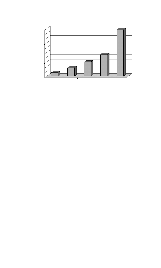
figure 1.2. Income Inequality in Nine Countries
as much income as the bottom 20 percent, and this is undeniably a
large discrepancy in terms of absolute size. To this point, however, we
have little in the way of context. How substantial is income inequality
in the United States in relative terms? One way to gain some perspective
on this question is to compare the United States to other countries.
5
Figure 1.2 shows the Gini
6
coefficient of income inequality in ten
countries for which comparable data were available in wave five of the
Luxembourg Income Study (LIS) – Switzerland, Poland, the Nether-
lands, Finland, Sweden, Germany, Norway, Canada, the United
Kingdom, and the United States. The data presented here show that
the United States has higher levels of income inequality than other
developed countries. While I focus here on just the countries available
in the most recent LIS data, neither the specific countries available for
analysis nor the measure of inequality used dramatically influences this
result. Comparative studies of income inequality consistently show that
inequality in the United States is among the highest of any developed
5
Achieving data-comparability in cross-national examinations of income inequality is
not easy. In fact, data-comparability problems limited scholarly comparative research
on income inequality for decades. Recently, many comparability problems have been
overcome, and the highest quality cross-national income data currently come from
the LIS.
6
The Gini ranges from zero to one with higher scores indicating more inequality.

Explaining Income Inequality
9
democracy (Brandolini and Smeeding 2006, Gottschalk and Smeeding
1997, Pontusson and Kenworthy 2005). Both our rich and our poor
are farther from the middle than in most other developed countries.
trends in u.s. income inequality
Thus far we have seen a snapshot of income inequality at the dawn
of the twenty-first century. If we wish to understand how political
dynamics influence distributional outcomes, however, we must move
beyond a cross-sectional snapshot. We need to examine how income
inequality has changed over time. Explaining the substantial movement
over time of inequality is the primary goal of the book.
To the degree that we can plumb it with the tools of economic
history, it is clearly the case that much of the twentieth century was a
time of major gains in income equality in the United States. Broken by
the Great Depression, the trend until 1973 was toward more income
equality. A surging industrial economy, the establishment of collective
bargaining over wages, and the labor shortages of four wartime periods
all helped to establish a society and economy in which the difference
between extremes of affluence and poverty was moderate – small by
historical standards.
Since 1973 (or some time in the early to mid-1970s) it is equally
clear that the trend has reversed. For more than three decades now,
most years in America have been less equal than the year before. Mod-
erated by the ups and downs of the economy, the underlying trend is
a march toward inequality. The America of the new third millennium
is substantially more unequal than its predecessor societies. Perhaps
more important, there is no indication in sight that the trend toward
greater income inequality has broken. Absent remarkable changes in
social and economic organization, it appears likely that the America of
decades to come will be one of stark differentials, perhaps one of two
societies with vastly divergent economic experiences.
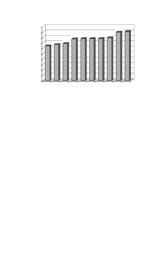
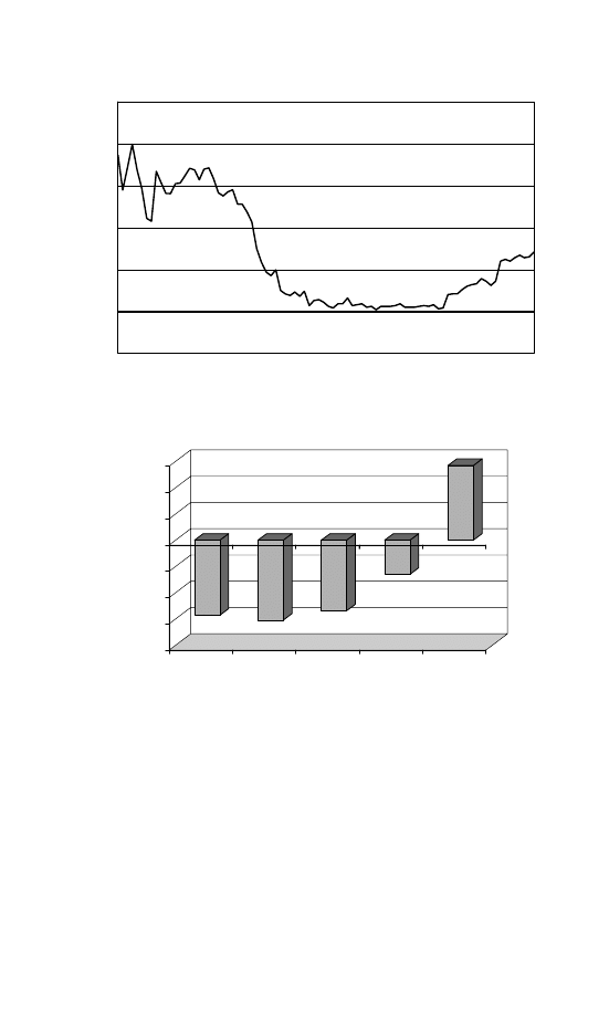
In Figure 1.3, I use a series provided by economic historians
(Plotnick et al. 2000) together with modern data on household incomes
from the Census Bureau to plot the path of the Gini from 1913 to 2000.
The Gini time series displays the pattern just described – a trend toward
equality (i.e., smaller values of Gini) disrupted by the turmoil of the
Great Depression and then continuing apace until the early 1970s. This
10
The Politics of Income Inequality in the United States
0.35
0.40
0.45
0.50
0.55
1913 1920 1927 1934 1941 1948 1955 1962 1969 1976 1983 1990 1997
Gini coefficient
figure 1.3. Gini Coefficient: 1913–2000
is followed by movement in the other direction, a growth of the Gini
(and the inequality it represents) from 1973 through the end of the
twentieth century.
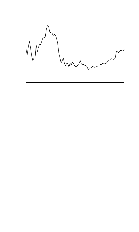
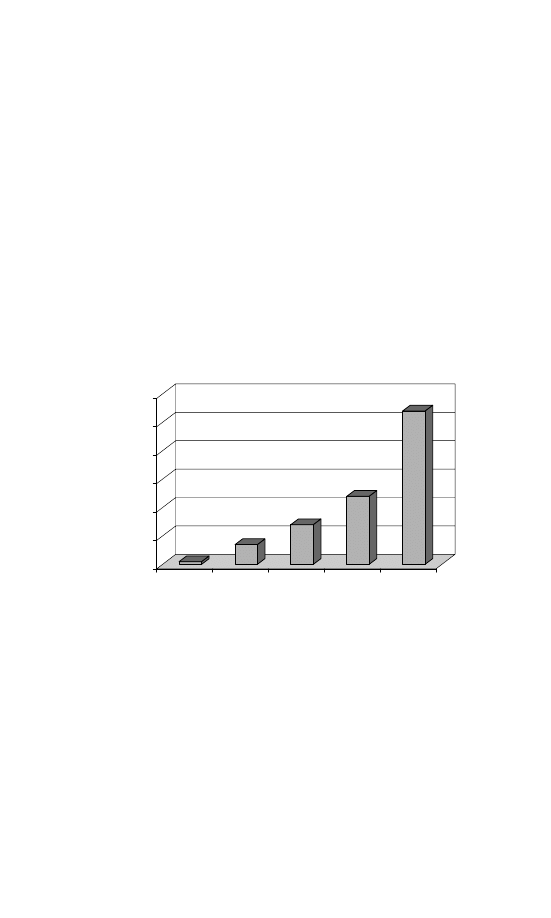
To get a somewhat different view of the matter, I look simply at how
much of the total national income is received by the upper 5 percent
of citizens (Figure 1.4). This simple descriptive statistic tells essentially
the same story. This highest income group received about a third of
all income early in the century. That share steadily declined into the
early 1970s to a level a little above 15 percent and then grew to about
22 percent by the century’s end. Thus the experience of the richest
Americans mirrors that of the whole distribution seen in the summary
Gini coefficient. Here, as with the Gini, the arrow points toward a
future in which Americans at the top will have an ever greater share of
the total income relative to those at the bottom.
The early 1970s was clearly a turning point in the story of equality
and inequality in America. So what happened? Who has been winning
and losing since this crucial reversal? To answer this question I examine
the experience of income classes over time.
7
Figure 1.5 shows how
7
It is useful to remember that income classes are not really “classes” in the sense of
impermeable boundaries. Not only do some people experience social mobility, but
many people experience mobility associated with age and life position. Professors, for
Explaining Income Inequality
11
10
15
20
25
30
35
40
1913 1920 1927 1934 1941 1948 1955 1962 1969 1976 1983 1990 1997
P
er
cent of total
figure 1.4. Income Share of Top 5 Percent: 1913–2000
–14.3%
–15.2%
–13.5%
–6.5%
14.2%
–20.0
–15.0
–10.0
–5.0
0.0
5.0
10.0
15.0
P
er
cent c
hang
e
1
2
3
4
5
Income quintile (lowest to highest)
figure 1.5. Changes in Income Share by Income Quintile: 1973–2000
the income share of each quintile changed between the beginning of
the inequality trend (1973) and 2000. Overall, the story is simple –
in relative terms, those at the top gained at the expense of everyone
else. The lowest income quintile began in 1973 with 4.2 percent of
aggregate income and ended in 2000 with just 3.6 percent – this is a
example, typically start their careers in quintiles 2 or 3 and complete them in the top
group.

12
The Politics of Income Inequality in the United States
14.3 percent decline. The story is similar for the bottom 80 percent
– between 1973 and 2000, the bottom four quintiles all experienced
a loss of income share. All of that loss was gained by the upper 20
percent, which began the era with 43.6 percent of aggregate income
and ended with 49.8 percent – a 14.2 percent increase.
theoretical foundations: political dynamics and
distributional outcomes
How can the path of income inequality in the last half of the twentieth
century be explained? Efforts to answer this question have come from
many disciplines, with some of the most commonly cited explanations
of income inequality based on sociological and economic theory – the
supply of or demand for skilled labor, business cycle fluctuations, tech-
nological change, single-female headed households, and rising female
labor force participation. Political science has also contributed to
this effort by examining the connection between social welfare pro-
grams and distributional outcomes (Hibbs and Dennis 1988, Page
and Simmons 2000). But those attempting to synthesize the literature
across disciplines have essentially concluded that the complex causal
processes underlying the distribution of income are not well under-
stood (Danziger and Gottschalk 1995, Jacobs and Skocpol 2005).
Intellectually, this is not at all satisfying.
The goal of this book is to test an empirical model of distributional
outcomes that explores the impact of aggregate level political dynam-
ics in addition to sociological and economic explanations. Here at the
outset, I describe this theoretical model in some detail so that it can be
used as a reference through the remainder of the book. I draw on pre-
vious work in two areas – U.S. macro politics and comparative welfare
states. Research in these traditions is related, but their development in
different fields of political science has produced little cross-fertilization.
By utilizing insights from both traditions, my work provides an impor-
tant bridge between work done in American and comparative politics
that leads to a fuller understanding of distributional processes.
From Mass Opinion to Societal Outcomes: The Macro
Politics Model
The theoretical foundation of my research begins with the macro pol-
itics model of the U.S. governing system. The macro politics model

Explaining Income Inequality
13
examines relationships between parts of the U.S. governing system
at the aggregate level such as public opinion, presidential approval,
partisanship, elections, and public policy. The argument is that the
parts of the system behave predictably and orderly. Citizens express
preferences about competing policy alternatives, the preferred alterna-
tives are enacted, and citizens then judge the quality of the outcomes
produced. A growing set of results in the macro politics literature
demonstrates systematic and understandable linkages between public
opinion, elections, and policymaking. Liberal shifts in public opin-
ion produce liberal shifts in policy because policymakers respond to
changes in public opinion and, if they do not, are replaced through
popular elections (Erikson et al. 2002, Page and Shapiro 1992, Stim-
son et al. 1995, Wlezien 1995). Simply stated, liberal public opinion
leads to liberal policymaking both directly and through election out-
comes. What we do not know is whether liberal policy making
leads to expected outcomes, in the aggregate. In other words, does
policymaking matter?
The fact that aggregate public opinion influences the course of pub-
lic policy in the United States is an important underpinning of my
model. But the macro politics model, in essence, assumes that the
changes in public policy produced by election outcomes and mass pref-
erences influence societal outcomes.
8
In the realm of income inequality,
a leftward shift in policy should produce different distributional conse-
quences than a move to the right according to the macro politics model.
However, this implication has not been broadly tested.
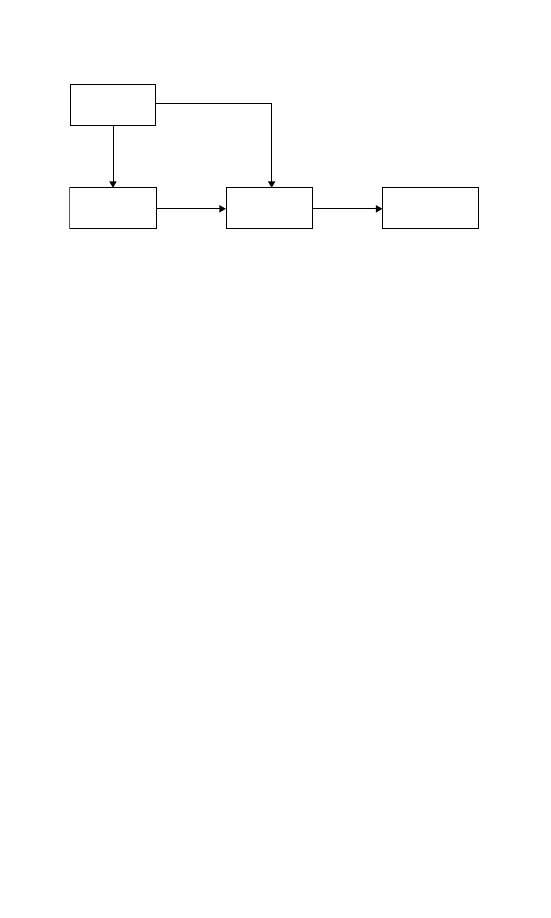
If citizens exert influence over public policy but policy does not
influence important societal outcomes, the substantive impact and the
normative implications of the opinion-policy link decline. Figure 1.6
depicts the macro politics model with an extension to distributional
outcomes. The connections between opinion, elections, and policy
are fairly well-known. The connection between policy dynamics and
distributional outcomes is not.
Studies too numerous to mention have examined the idea that gov-
ernment policies have distributional implications, but my approach
makes a unique contribution. The effect on poverty and inequality of
public education, health benefits, social insurance, public assistance
programs, and taxes have been discussed time and again (Page and
8
Though see Kellstedt et al. (1996) for evidence of policy’s influence on racial equality.
14
The Politics of Income Inequality in the United States
Policy Mood
Election
Outcomes
Policy
Liberalism
?
Income Equality
figure 1.6. The Macro Politics Model and Distributional Outcomes
Simmons 2000, Pechman and Okner 1974, Pechman 1985). However,
the existing discussion of public policy and distributional outcomes
is largely based at the micro level (though one notable exception is
provided by Kellstedt et al. (1996)). That is, the questions revolve
around the impact of individual policies or policy domains. Rather
than focusing only on the distributional impact of individual policies,
I examine policy at the macro level – that is, collectively across issues
and policy domains. While the micro perspective often sees policy
enactments as the result of idiosyncratic forces specific to individual
proposals, the macro perspective views policy as the systematic prod-
uct of more general ideological and partisan conflicts that cut across
issues. Given the centrality of distributional outcomes to political con-
testation, there should be a connection between macro policy and
distributional outcomes.
Who gets what according to the macro politics model? According
to this view, it is a consequence of aggregate political dynamics. The
preferences of the mass public, who gets elected to office, and the
policies enacted by policy makers should all play a role. This book
provides an empirical assessment of whether this is the case.
Comparative Insights on American Inequality
Given that previous analyses of the macro politics model have not
examined the distributional consequences of political dynamics, I turn
to the welfare state literature to flesh out the mechanisms through
which aggregate level political phenomena might influence distribu-
tional outcomes. The state-centric model (Skocpol and Amenta 1986),
the logic of industrialism (Pampel and Williamson 1988, Wilensky

Explaining Income Inequality
15
1975), and power resources theory (Esping-Andersen 1990, Huber
et al. 1993, Huber and Stephens 2001, Korpi 1978, 1983, Stephens
1979) are the three leading theories of welfare state development.
Each of these theories suggests different factors as influential in
determining distributional outcomes. The state-centric model focuses
on institutional structure and bureaucratic preferences, the logic of
industrialism focuses on demographic and economic conditions, and
power resources theory emphasizes the strength of lower class power
resources in the form of left political parties and labor unions. Each of
these theories informs the analysis in this book, but power resources
theory has been cited as the dominant explanation of welfare state
development in the extant comparative literature (Orloff 1996) and
thus, is most central to my theoretical argument.
Power resources theory is rooted in the idea that the upper and lower
classes have divergent distributional preferences, with the lower class
favoring more egalitarian outcomes than the upper class. The theory
goes on to argue that the lower classes must organize in order for their
collective voice to be heard and influence outcomes. Power resources
are the factors that facilitate organization, and the theory conceptual-
izes two realms in which the lower classes can organize – the economy
and politics. Organization in the economic realm is evidenced by labor
union strength, and organization in the political sphere is evidenced by
the strength of left parties in government. Left-party control and union
strength, in turn, influence distributional outcomes. Figure 1.7 depicts
these connections.
The most important idea that I borrow from power resources theory
is that distributional outcomes can be influenced through the market
and through the government. Note in Figure 1.7 that market power
Lower Class
Power
Resources
Party
Control
Union
Strength
Market
Decisions
Income
Distribution
Explicit
Redistribution
figure 1.7. The Traditional Power Resources Model of Distributional
Outcomes
16
The Politics of Income Inequality in the United States
resources evidenced by labor union strength produce an impact on
market decisions and that political power resources evidenced by left
parties influence state activity. Both state activity and market deci-
sions, in turn, influence income inequality. As we will see in a moment,
this idea becomes central in my overarching model of distributional
outcomes in the United States.
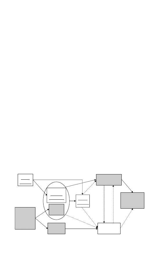
A Combined Model of Distribution and Redistribution
The model of distributional outcomes analyzed in this book is pre-
sented in Figure 1.8. In part, this model is an explicit combination
of the macro politics model and power resources theory. The chart
demonstrates that there is a fundamental connection between these
two theories. First, focus on the oval in the middle of the diagram.
In the parlance of the macro politics model, “election outcomes” are
discussed, while “party control of government” is utilized in the ver-
nacular of power resources theory. These phrases express a similar
concept, linking the two theories theoretically and empirically by a
common component. Both theories are concerned with which political
team controls the policymaking apparatus. Linking the two provides
a comprehensive theoretical framework to analyze the macro political
dynamics of income inequality in America.
This overarching model extends previous work in the macro poli-
tics and power resources traditions considered separately and provides
Public
Opinion
Party
Control
Union
Strength
Lower Class
Power
Resources
Election
Outcomes
Public
Policy
‘‘Market’’
Inequality
Post-
Government
Inequality
Explicit
Redistribution
figure 1.8. The Overarching Model: Combining Macro Politics and Power
Resources

Explaining Income Inequality
17
unique contributions to our general understanding of distributional
processes. The shading of the boxes and the type of line connecting
each component draw attention to the novel aspects of the model. The
underlined text boxes show the key components of the macro poli-
tics model and the shaded text boxes represent components of power
resources theory. The solid arrows between boxes show relationships
that have been previously discovered, while the dashed arrows indicate
connections that will be assessed for the first time in this book.
With reference to the U.S. macro politics literature, this model is
in part a straightforward extension. Existing research generally does
not examine the implications of policy shifts for societal outcomes.
My model broadens this work through an explicit examination of
the distributional implications of macro policy. Note here the lines
connecting public policy to market inequality and redistribution. By
implication, this extension of the macro politics model also provides
for an assessment of popular influence over societal outcomes.
The theoretical extension of the macro politics model, however,
goes beyond merely extending the analysis to assess whether policy
affects the dynamics of inequality. I also examine how inequality rever-
berates back into the system. The figure contains arrows between
market inequality and redistribution. Inequality and redistribution, as
the key distributional outcomes analyzed in this book, are not just
outcome variables, but also matter as a causal factor in their own
right. The model posits that market inequality influences the choice
of redistributional policies enacted and that the amount of redistri-
bution achieved by government also affects market inequality. This
places gains and losses in economic equality squarely within the sys-
tem of American political dynamics, as both a consequence and a
cause.
The contribution to power resources theory is a bit more nuanced.
First, I add public policy as an explicit component of the power
resources model. Previous research has not distinguished policymak-
ing as a distinct causal stage. In existing work, party control leads
directly to redistribution. Most proponents of power resources theory
likely believe that party control is translated into societal outcomes
via policy activity, but this has not been empirically examined in the
comparative literature. Probably due in large part to a lack of com-
parable cross-national data, comparative research relies on observing

18
The Politics of Income Inequality in the United States
the connection between power resource variables and policy conse-
quences like government redistribution, rather than directly observing
policy itself.
9
I bring public policy into the power resources model as
an indicator of power resources, with left policies indicating greater
lower class power resource mobilization.
The second extension of power resources theory is the connection
between power resources and market decisions. Following the lead of
Bradley et al. (2003), I conceptualize and measure the distributional
process in two stages. The first stage is driven primarily by private
market decisions. Firms decide how much to pay their employees,
individuals make investment decisions, and the price of commodities
fluctuates. All of these private decisions bear directly on the market
distribution of income. The second stage of the process is where gov-
ernment becomes explicitly involved by redistributing income – taking
money from some and giving it to others. Based on previous work in the
power resources literature, we would be forced to conclude that politi-
cal dynamics matter only in the second stage – redistribution. Political
power resources (left parties) induce greater redistribution, and mar-
ket power resources (labor unions) induce lower market inequality.
I add to power resources theory by exploring the possibility that polit-
ical power resources influence not only redistribution but also market
inequality.
The impact of political power resources on market inequality would
occur via what I label a “market conditioning” mechanism. In general,
market conditioning refers to any situation in which private market
decisions that can be readily observed are influenced by government
action. Does government influence market decisions? This almost goes
without saying.
Large swaths of the tax code are designed for this very purpose.
Tax deductions for mortgage interest, charitable contributions, health
care, and business capital expenditures all influence private decisions.
The mortgage tax deduction provides a classic example. By virtue of
the fact that interest payments on home mortgages are deductible from
9
Some comparative work appears to muddle the line between policy and outcomes by
using policy decisions such as social welfare expenditures as an indicator of redis-
tribution. I define redistribution as impact rather than just effort, and policy as the
governmental decisions that are designed to influence society.

Explaining Income Inequality
19
taxable income, home ownership is subsidized. At the margin, more
homes are purchased because of this provision in the tax system. And
in this case, those with high incomes tend to benefit the most.
Examples of market conditioning go far beyond tax expenditures.
Job training programs provide skills to individuals that augment their
employability. There are people currently employed who would not
have been able to find jobs without previous experience in such
training programs. Some people probably make investment decisions
that they would not have made without government-required cor-
porate reporting. Think also about how government construction
of the interstate highway system has conditioned market outcomes.
Railways became less prevalent, logistics companies began focus-
ing on over the road applications, and businesses moved nearer to
interstate hubs.
The common thread in all of these examples is that the market out-
come we observe is different than it would be in a hypothetical world
without government. Recent work in the American politics literature
has begun to focus attention on government policies that condition
market outcomes (Howard 1999, Page and Simmons 2000). It may
even border on the tautological to say that government conditions mar-
ket outcomes. That much is a given. Whether the market conditioning
impact of government has implications for income inequality is another
matter. I ask whether market conditioning has a systematic impact on
the gap between rich and poor and whether this impact responds to
macro political dynamics. If left parties and policies tip the scales of
government conditioned market inequality in favor of the poor, this
is evidence that market conditioning does influence income inequal-
ity systematically and in the direction predicted by power resources
theory. Analyzing market conditioning as a potential mechanism for
governmental influence on distributional outcomes represents a major
theoretical advancement on current versions of power resources theory
and the general literature on income inequality.
Who gets what? The central theme of the book is that government is
an important determinant of the answer. I show that when the political
landscape changes – a different party takes over the White House, the
ideological direction of public policy shifts, or the mood of the pub-
lic changes – income inequality responds in consistent and predictable
ways. Shifts to the left produce more egalitarian outcomes and shifts to

20
The Politics of Income Inequality in the United States
the right exacerbate existing inequality. Economic conditions matter
for distributional outcomes, but I also demonstrate that political
dynamics matter at least as much, and that the influence of politics man-
ifests itself in some surprising ways. We expect government to influence
distributional outcomes via explicit redistribution, but government
also shapes income inequality by conditioning market outcomes. In
fact, this mechanism of distributional impact is at least as strong as,
and works in tandem with, redistribution.
an outline of the book
I pick up the story of government’s role in equality and inequality in
America in Chapter 2, where I introduce the theme of government’s
distributional impact. I discuss the policies that are most readily associ-
ated with income redistribution – tax and transfer programs. I compare
the redistributional effect of programs such as Medicare, Social Secu-
rity, unemployment benefits, and cash assistance policies. Then, I go on
to discuss a second broad category of policies that can influence distri-
butional outcomes via market conditioning. I argue that programs that
do not explicitly redistribute income may be a particularly important
part of the story in the United States.
The central message of Chapter 3 is that ideological and partisan dis-
agreement over distributional outcomes is considerable in the United
States. The first part of the chapter utilizes the debate over the mar-
riage penalty tax in 2000 as a case study in distributional conflict. This
tax policy provides a perfect example of political conflict over a pol-
icy with explicit distributional consequences, but one which was not
broadly perceived as being primarily about income inequality. In the
case study, I analyze the distributional differences between Republican
and Democratic proposals, provide excerpts of floor debate address-
ing the distributional conflict, and draw on interviews I conducted with
specific members of Congress. The second part of the chapter presents
findings from a survey of members of Congress. I tentatively find
that there are ideological and partisan disagreements in terms of the
relative importance of distributional outcomes compared to other eco-
nomic considerations. There are also differences regarding appropriate
forms of government action to equalize both economic opportunity and
outcomes.

Explaining Income Inequality
21
Chapter 4 addresses one of the central questions of the book:
Do national election outcomes influence distributional outcomes? I
develop the overtime measures of inequality that will be central to the
remainder of the analysis. I also discuss power resources theory in the
context of the American case. I argue that convincing explanations of
income inequality must account for politics in a systematic way. I then
examine the effect of partisan control of the House, Senate, and pres-
idency on redistribution and market income inequality from 1947 to
2000. I find that Democratic control of government not only influences
explicit redistribution, but also influences market inequality.
The theme of assessing the connection between political dynamics
and income inequality continues in Chapter 5, where I shift my focus
from party dynamics to policy dynamics. This chapter is similar in
organization to Chapter 4. I discuss why an examination of partisan
control is only part of the picture and that an analysis of the poli-
cies produced by different partisan constellations of power is needed.
I discuss the macro politics model in detail and show how my work
extends existing research in an important direction – to an analysis of
the substantive impact of policymaking. I find that shifts toward the
left in public policy produce reductions in inequality. These reductions
occur both because of more redistribution and because of reductions
in inequality prior to taxes and transfers. I conclude based on this evi-
dence that market conditioning as well as explicit redistribution are
important political determinants of income inequality in America.
Chapter 6 links the analyses of the previous chapters together into
a comprehensive analysis of income inequality in the United States. In
the first part of this chapter, I answer the following questions: What
is the total impact of politics on distributional outcomes? Is there a
reciprocal linkage between redistribution and market inequality? Do
mass preferences influence distributional outcomes? I find that the
overall impact of politics rivals that of many economic factors and
that market inequality and redistribution are interconnected. Redistri-
bution drives market inequality higher, but lower market inequality
drives redistribution down. I show that Democratic Party control of
the White House and left policymaking reduce overall inequality, while
surprisingly reducing explicit redistribution at the same time. I also
demonstrate that public opinion has an important indirect influence
on distributional outcomes via its influence on policymaking.

22
The Politics of Income Inequality in the United States
In Chapter 7, I discuss the future of income inequality in America
and summarize the major findings of my research. I argue that the find-
ings in this book, when coupled with what previous studies of the U.S.
macro polity have taught us, show that political dynamics are central to
distributional outcomes. More specifically, changes in mass attitudes
produce changes in public policy through representational linkages.
These changes in policy, in turn, substantively influence outcomes in
the realm of income inequality. Thus, citizens can exert influence on
an important contested outcome through democratic politics in the
United States.

2
The Distributional Force of Government
Now as much as ever, government is pervasive. Regardless of values
like liberty and freedom and limited government, the state influences
numerous aspects of life. In nearly every recent national election cam-
paign, we have seen candidates propose divergent policies on topics
ranging from coal-fired power plants, to fuel efficiency standards, to
national carbon emission targets, to provision of health insurance,
to family planning policies, to educational goals, to free trade, and
to employment policy. Government enacts policies ranging from the
social sphere, to the economic sphere, to the environment, and so on.
But what difference do government policies make for distributional
outcomes?
In this chapter I focus on two major questions. First, what govern-
ment activities have the potential for influencing income inequality?
Second, how much impact do these policies have? Specifically, I dis-
cuss two broad mechanisms through which government can influence
the distribution of income: explicit redistribution and market condi-
tioning. I also discuss a straightforward strategy for measuring the
influence of redistribution. Using income data from 2000, I examine
the distributional effects of a wide variety of redistributional programs.
mechanisms of distributional impact
There are any number of policies and programs that could be used
to influence distributional outcomes. Many programs are clearly and
23

24
The Politics of Income Inequality in the United States
closely tied to efforts to balance the scales between rich and poor.
But these sorts of programs comprise only a portion of government
activities in the United States. Politicians from both sides of the aisle
are reticent to speak of redistribution – at least not with a positive
tone. But if the question of “Who gets what?” is central to politics,
there is likely more to the distributional impact of government than
just policies explicitly aimed at balancing the scales of inequality.
Explicit Redistribution
When people think about programs that influence income inequality,
the programs most likely to come to mind are explicitly redistributive
– programs that take money from some (in the form of taxes) and give
to others (in the form of benefit payments). Even the relatively small
traditional welfare state operated in the United States includes a variety
of redistributive programs, ranging from welfare to Social Security. The
focus here is government policies that explicitly redistribute income
from the top of the income distribution toward the bottom. What we
want to know is the degree to which explicit government redistribution
equalizes incomes in the United States.
The redistributive effect of a government program is straightfor-
ward in concept. It is the difference between the hypothetical income
inequality that would exist in the absence of government activity and
the income inequality that exists after government has acted. The
empirical observation of this concept is, however, quite difficult. While
income inequality as it has existed in the United States for the past
several decades can be observed, a world in which government has
not played a role simply does not exist. Thus, the full implications
of government action on income distribution can be only imperfectly
observed.
Many federal government programs influence the distribution of
income. Some have effects that are hard to pinpoint. Other programs
affect the distribution of income through either cash or in-kind ben-
efits, and these are the kinds of programs I look at in this section.
Food stamps, Social Security, Medicare, and a variety of other bene-
fits fall under this category. But expenditures are only one side of the
coin. Taxes have distributional consequences as well. While it is diffi-
cult or impossible to observe the full distributional effects of explicitly

The Distributional Force of Government
25
redistributive programs, available data can be used to measure the
direct effects of government taxation and explicit benefits.
Consider the effects of Medicare in order to illustrate the idea of
direct, first-order effects of a program as opposed to indirect, higher-
order effects that are extremely difficult if not impossible to observe.
The direct beneficiaries of Medicare are the elderly who seek medi-
cal care. It is simple enough to calculate the distributional impact of
Medicare for these beneficiaries. Calculate household income exclud-
ing the value of Medicare benefits and compute inequality based on
this income concept. Then calculate income including the value of
Medicare benefits and measure the degree of inequality. The first-order
effect of Medicare on inequality is the difference between pre-Medicare
income inequality and post-Medicare income inequality. But how
would the income of doctors be changed if Medicare did not exist?
This is a question that cannot be answered empirically because we
do not and cannot know (without myriad assumptions) what a physi-
cian’s income would be in the absence of Medicare. It could be lower
because some elderly might skip medical care without Medicare, but
it could also be higher if doctors did not fill parts of their sched-
ule with Medicare patients who, via government reimbursement to
the physician, pay below-market rates for many procedures. Similar
issues arise with welfare programs that may dissuade work effort at
the same time that they provide cash to beneficiaries. It is difficult to
know with precision exactly how much work is reduced by the receipt
of benefits. When calculating distributional impact, then, I focus on
what can be known – the direct, first-order impact of government
programs.
In order to calculate the explicit distributional effect of a government
program, the distribution of income excluding the program must be
compared to the distribution of income including the program. The
first step in calculating the distributional consequences of government
programs is to define a baseline income distribution as a consistent
point of comparison. This distribution should include only income
that comes from market (nongovernmental) sources. Fortunately, with
individual-level March CPS data, this task is straightforward.
In the previous chapter the focus was on household money income
inequality. But money income, as an income concept, includes income
from only a handful of government programs like public assistance that
26
The Politics of Income Inequality in the United States
distribute benefits in the form of cash payments. This excludes in-kind
benefits, like Medicare. So money income is not a sufficient income
concept for the purpose of determining the distributional impact of
individual government programs. As a baseline for comparison, I will
focus on income excluding money from any government mandated,
funded, or administered program. I call this concept pre-redistribution
income, and it includes income from the following sources: earnings
from an employer, employer health care contributions, capital gains,
pension or retirement income, interest, dividends, rents, royalties,
estates, trusts, alimony, child support, financial assistance from outside
the household, and other money income that is not otherwise cate-
gorized.
1
Figure 2.1 shows the aggregate share of pre-redistribution
income for each income quintile in the year 2000.
1%
7%
15%
24 %
53%
0
10
20
30
40
50
60
Percent of aggregate
incom
e
1
2
3
4
5
Income quintile
figure 2.1. Income Distribution by Quintile for Pre-Redistribution Income
1
One could argue that other governmental sources of income should also be excluded.
For example, federal employees obviously receive their wages from the government. I
view this type of government income source differently than government sources that
provide payments (or mandate employer payments) for something other than labor.
There are certainly some gray areas in this categorization. For example, workers’
compensation income is not included in pre-redistribution income. Workers’ compen-
sation is paid jointly by the government and the injured worker’s employer. Because
it is a government mandated program that is at least partially funded out of govern-
ment coffers, I exclude it from pre-redistribution income. On the other hand, child
support payments are also, in a sense, mandated by government. However, these pay-
ments come completely from private funds and are thus included in pre-redistribution
income.

The Distributional Force of Government
27
We see in this figure that, prior to any explicit redistribution by
government, the top income quintile held more income in 2000 than
the bottom 80 percent of households combined. Measuring inequality
excluding government benefits is the first step toward assessing the dis-
tributional consequences of government programs, and inequality in
pre-redistribution income provides a baseline for assessing the distri-
butional consequences of government programs in the United States.
The second step is to determine how the distribution of income changes
when benefits from a particular government program are reintroduced
to the definition of income. In the sections that follow, I examine
how taxation and benefit programs influenced income inequality in
the United States during the year 2000.
The Distributional Impact of Taxation
There is no shortage of political debate and rhetoric about the fed-
eral government’s system of taxation. On the one hand, Republicans
almost always have some proposal in the works to flatten taxes so that
everyone pays their “fair share,” which in the eyes of many conserva-
tives means all paying the same proportion of their income in taxes.
Democrats, on the other hand, often bemoan the lack of fairness in
the U.S. tax code that allows wealthy individuals to dodge taxes. The
liberal viewpoint is that the tax system is weighted too far in favor of
the rich. But what is the real story?
The national government in the United States collects several forms
of taxes.
2
In terms of those that directly influence the amount of income
taken home by U.S. households, these forms of taxation fall principally
into two categories – income taxes and payroll taxes. Income taxes, as
all of us in America are acutely aware, are based on the amount of
income earned within a household. As one earns more money, the
amount of taxes due on each additional dollar earned increases. The
federal income tax, then, is in theory a progressive tax that takes greater
percentages from those who earn large sums of money than from those
2
My focus here is almost entirely on taxes collected by the national government. State
and local governments also collect a variety of taxes, and some taxes collected at the
state level are notoriously regressive, such as the sales tax. My analysis here does
not account for taxes at all levels of government, but others have conducted detailed
analyses of state and local taxation (Peppard and Roberts 1977).

28
The Politics of Income Inequality in the United States
who earn little. Of course the federal income tax is much more com-
plicated than a simple increasing marginal tax rate. Tax liability is
reduced for those with expenditures on items ranging from higher edu-
cation to home mortgage interest to hybrid gas/electric vehicles. All of
these deductions reduce taxable income, thereby reducing taxes paid.
Most deductions, in fact, are likely to benefit middle and upper income
households (like the mortgage interest deduction). Other programs that
are part of the federal income tax system are explicitly designed to help
the working poor (like the Earned Income Credit).
3
Payroll taxes are somewhat different than income taxes. Payroll
taxes, as the name implies, are taxes collected based on how much
an employer pays each employee. The major federal payroll taxes are
Social Security, Medicare, and unemployment insurance. Payroll taxes
are determined as a percentage of wages paid to an employee, but part
of the tax is paid by the employee and part is paid by the employer. Fur-
thermore, for both Social Security and unemployment, taxes are paid
only until the employee earns a specified amount. In 2000, for exam-
ple, employees were required to pay 6.2 percent of the first $76,000
of their wages in Social Security tax, with a matching amount paid
by employers; amounts above that are not taxed. Medicare taxes are
apportioned via a flat rate that is shared by the employer and employee
with no earnings ceiling for the tax. Finally, unemployment taxes are
fully paid by the employer.
It should be fairly obvious that a tax structured like Social Security
will be regressive, taking a greater percentage of earnings from workers
with little income than from those high in the income distribution. Two
earners making $76,000 and $7,600,000, for example, pay identical
dollar amounts of Social Security taxes. I am interested primarily in
the direct effects of payroll taxes paid by the employee. Of course, at
least a part of the employer’s portion of payroll taxes can be shifted
3
Revenue lost by the federal government because of available deductions and programs
like the Earned Income Credit (EIC) are called tax expenditures. Tax expenditures are
a common way for government to give benefits to certain groups without having a fiscal
expenditure in terms of the government balance sheet. I treat tax expenditures as a part
of the tax system, but these government benefits are no different than others in the sense
that they can help some groups more than others, thereby influencing the distribution
of income. However, I do not conduct detailed analyses of the distributional effects
of individual tax expenditures, though others have (Howard 1999).

The Distributional Force of Government
29
table 2.1. Distribution of Federal Taxes and Earned Income Credit,
2000
Pre-Redistribution Quintile (%)
Type of Tax
1
2
3
4
5
Federal Income
0
3
8
18
71
Federal Payroll
1
8
17
26
48
Earned Income Credit
15
61
15
6
2
Total Federal Taxes
0
3
11
21
65
Share of Pre-Redistribution Income
1
7
15
24
53
to the employee in the form of reduced wages. However, I view this
as an indirect effect of the tax program that varies by employer. In
fact, most economists studying this issue find that employer payroll
taxes are only partially shifted to employees (Beach and Balfour 1983,
Holmlund 1983, Vroman 1974, Weitenberg 1969).
In Table 2.1, I begin to explore the distributional effects of several
tax programs. This table shows the proportion of federal income and
payroll taxes paid and Earned Income Credit (EIC) received by each
pre-redistribution income quintile. A completely proportional tax (or
credit) would be allocated between the income quintiles in the same
proportion as pre-redistribution income. Not surprisingly, the first row
of the table shows that federal income taxes are progressive. While the
top income quintile has 53 percent of all pre-redistribution income,
households in this quintile pay 71 percent of federal income taxes. The
opposite is true for the first four quintiles.
We see in the second row that federal payroll taxes are regressive not
only in design but in distributional impact. The bottom four income
quintiles pay a larger proportion of their income in payroll taxes than
does the top quintile. The most prominent part of the tax system that
is designed to equalize incomes through aid to low and middle class
working families (the Earned Income) clearly distributes benefits in a
manner consistent with this goal. More than three-quarters of Earned
Income benefits go to the bottom two income quintiles.
4
If we look
4
On its face it is difficult to understand how less than 100 percent of Earned Income
benefits go to the lowest income quintile. The income cutoffs for Earned Income
eligibility for families with children, however, go well into the second quintile. In
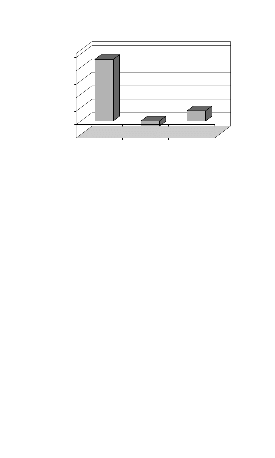
30
The Politics of Income Inequality in the United States
4.6%
–0.4%
0.8%
–1.0
0.0
1.0
2.0
3.0
4.0
5.0
Percent reduction in
Gini
Federal income
Federal payroll
Earned income
credit
figure 2.2. Reduction in Inequality Attributable to Federal Tax Programs in
the United States
at the final two rows of the table, it is clear that the federal tax sys-
tem appears to be at least moderately progressive – taking a greater
percentage of income from the rich than from the poor. This is espe-
cially noticeable at the top of the income distribution, where the top
quintile pays 65 percent of all federal taxes but holds 53 percent of all
income.
The tangible effect of federal taxes on income inequality during the
year 2000 is examined in Figure 2.2. This chart shows the percent
reduction in the Gini coefficient that can be attributed to the forms of
taxation discussed above. The federal tax program that has the single
largest effect on income inequality is the federal income tax, which
reduced income inequality from its pre-redistribution level by 4.6 per-
cent during 2000.
5
The Earned Income Credit also equalizes incomes,
but by a much smaller amount – less than 1 percent. Federal payroll
addition, even a few households in the higher quintiles can receive benefits due to
differences between households and tax units. People in the same household (an adult
child and parent, for example) can be taxed separately. Thus, a child of a high-income
parent may qualify for the Earned Income despite the fact that household income is
in the upper part of the distribution.
5
This calculation, of course, does not include reductions in work effort, since it is
calculated simply by computing inequality in income with taxes included as income
and then again after subtracting taxes from income. Those at the top might have
earned more pre-tax income were it not for the deterrent effects of a progressive
marginal tax rate.

The Distributional Force of Government
31
taxes, on the other hand, slightly increase inequality in the United
States, and this result is driven primarily by the Social Security tax.
6
The Distributional Impact of Government Expenditures
Federal taxes have some impact on the distribution of income, but the
programs with the most readily apparent distributional consequences
involve government expenditures. The programs that many Ameri-
cans would probably name if asked which government programs give
the most help to the poor would be means-tested programs – benefits
like food stamps and welfare. These programs are specifically targeted
toward the needy because an individual must be below a certain income
level before attaining eligibility for the program. But means-tested pro-
grams make up a relatively small part of the national budget, much
less than 5 percent, in fact. I begin my discussion of the distributional
impact of expenditures with two large non-means-tested programs that
are designed to ease the financial burden of the retired – Social Security
and Medicare.
Social Security and Medicare
In some of the political commentary of the last two or three decades the
twin retirement security programs, Social Security and Medicare, have
been pictured as boondoggles for the newly affluent “senior” class.
Designed as unabashed income redistribution schemes by Franklin
Roosevelt and Lyndon Johnson, the two programs have ballooned
dramatically as the numbers of retiree recipients have grown with an
ever-increasing American life-span and will likely grow further as baby
boomers enter retirement. It is commonly suggested that the programs
have become entitlements for a politically influential group which,
though it no longer needs the benefits, has life-and-death control over
the policymakers who decide what to do. One can imagine a por-
trait along the lines of Ronald Reagan’s famous “welfare queens,” the
6
More comprehensive tax incidence studies that examine state, local, and federal
taxes that are not levied on individuals (like taxes on business profits) argue that
the overall distributional effect of taxation in the United States is very minimal
(Pechman 1985, Pechman and Okner 1974). The distribution of the tax burden is
essentially proportional except for the richest and poorest households.
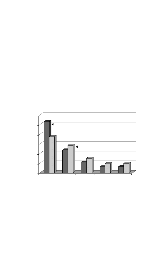
32
The Politics of Income Inequality in the United States
silver-haired retiree driving his Mercedes Benz to the country club,
stopping off to deposit the monthly Social Security check.
Reality, however, is quite contrary to this image. The data on Social
Security and Medicare recipients presented in Figures 2.3 and 2.4 tell
the real story. Recipients are, for the most part, still the poorest Amer-
icans. And the income from these programs is for most of these people
virtually all the income they have. Fifty-three percent of total Social
Security benefits go to those in the lowest pre-redistribution income
quintile, and only 23 percent of these benefits go to the top three
quintiles combined. The distribution of Medicare benefits is similar,
though not quite as skewed as Social Security.
7
The bottom 40 per-
cent of households receive 66 percent of these benefits, and the top two
quintiles garner only 19 percent. Clearly, Social Security and Medicare
53%
37%
24%
29%
11%
15%
6%
9%
6%
10%
0
10
20
30
40
50
60
Percent share of benefits
1 2 3 4 5
Pre-redistribution quintile
Social security
Medicare
figure 2.3. Share of Social Security and Medicare Benefits Received by Each
Income Quintile
7
Medicare is a noncash benefit that provides those over 65 with access to medical care.
Since this benefit is not in the form of cash, there is some question about how to convert
the benefits received into income. The March CPS values Medicare benefits using the
fungible conversion method. Rather than converting Medicare benefits to income by
computing the market value of the health care received, the fungible method determines
the amount of money the household would have actually spent on health care had the
benefit not been received. The assumption of this method is that households would
have forgone health insurance if given the choice between food and insurance. So, the
fungible method provides a conservative method for determining the redistributive
effect of Medicare.
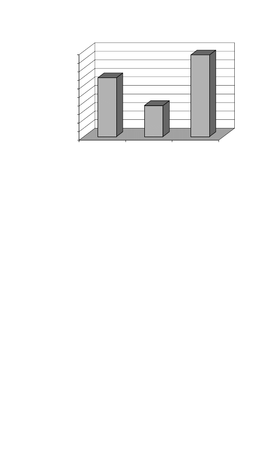
The Distributional Force of Government
33
10.0
6.9%
3.6%
9.6%
P
er
cent reduction in
inequality
9.0
8.0
7.0
6.0
5.0
4.0
3.0
2.0
1.0
0.0
Social security
Medicare
Combined
figure 2.4. Reduction in Inequality Attributed to Social Security and Medi-
care Benefits
cannot be fairly characterized as a boon for the wealthy. In fact, this
draws attention to the reason why many people in America are poor
– they are old and can no longer work. To be perfectly clear, much
of the bottom quintile is composed of individuals over age 65 who
are retired. These are the primary recipients of the largest government
benefit programs.
The equalizing effects of Social Security and Medicare are quite dra-
matic, so much as to dwarf all other federal programs. If the level of
inequality after Social Security and Medicare (each treated separately)
are compared to pre-redistribution inequality, we see that Social Secu-
rity benefits reduce inequality by nearly 7 percent and Medicare reduces
inequality by 3.6 percent (see Figure 2.4). When the effect of both pro-
grams is combined, the Gini coefficient drops from 0.52 to 0.47, a
reduction of almost 10 percent. Examining just these two programs
clearly shows that the greatest redistributive impact of government
in the United States comes through expenditures rather than revenue
collection. Without these two programs, nearly one-fifth of all Ameri-
cans would essentially have no income.
8
These individuals would lack
8
Some of these individuals would elect to continue working, but at some point this
would obviously become impossible. Furthermore, it is hard to imagine that many
people who subsist on Social Security and Medicare alone would not seek other forms
of income under the current plan if they could. These benefits do not exactly provide
for kingly living, but do allow elderly Americans to subsist during their retirement
years.

34
The Politics of Income Inequality in the United States
income for food and housing and would then incur medical expenses
(often associated with aging). However, they would not be able to pay
for these expenses nor could they afford insurance to replace Medi-
care. This is not the welfare state that is the centerpiece of political
dialogue. In dollar terms, however, it is the welfare state that mat-
ters. Everything else – particularly income assistance programs targeted
toward the poor and the unemployed – is at the periphery. I turn now
to describing the effects of those “other” programs.
Other Programs
The programs discussed in this section are an interesting combina-
tion of federal, state, and local activities, so isolating the effect of
the national government in these programs is impossible. For exam-
ple, Medicaid (the medical program for the poor) was initiated by the
federal government, but is administered and partially funded by the
states. States get to decide specific eligibility criteria and benefit levels,
with funding shared by the national government. Some states would,
no doubt, have similar programs without funding from the national
government, but it is likely that funding levels would be lower and
many states would forgo such programs completely. Strictly speaking,
the effects of programs like Medicaid should be allocated between the
state and national governments. However, I do not have any basis on
which to make such an allocation with the data I am using. Therefore,
I attribute the distributional effects of these programs to the federal
government alone.
It would be desirable to array the redistributive effect (percent
decrease in Gini attributable to income from each program) of all
spending programs on a single graph such as Figure 2.4. But Social
Security and Medicare had to be treated separately because their scale
is so great that other programs look trivial in contrast. The programs
are not trivial, and we can see in Figures 2.5 and 2.6 that some matter
more than others.
Figure 2.5 shows the reduction in inequality that non means-tested
benefit programs have in the United States. These are programs that
have no income requirement for eligibility. In order to receive benefits
from these programs, one has to be in a specified category of individ-
uals, with these categories not being defined by income. To receive
veterans’ benefits, one must have fought in a foreign conflict for the
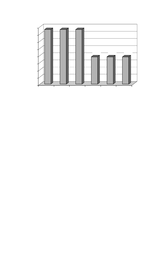
The Distributional Force of Government
35
0.4%
0.4%
0.4%
0.00
0.05
0.10
0.15
0.20
0.25
0.30
0.35
0.40
Percent reductionin
inequality
Veterans Survivor Disability Unemp-
loyment
Workers’
comp.
School
lunch
0.2%
0.2%
0.2%
figure 2.5. Equalizing Effect of Non-Means-Tested Government Benefit
Programs
U.S. military. To receive school lunches, a household must have chil-
dren attending a school that participates in the school lunch subsidy
program.
9
The distributional impact of veterans’, survivor, and dis-
ability benefits are similar, with each program reducing inequality by
approximately 0.4 percent. Unemployment benefits, workers’ com-
pensation, and the school lunch program have an even smaller effect,
reducing inequality by about 0.2 percent each.
Still, all of the programs discussed to this point are not what most
Americans probably think of as the American welfare state. Rather,
welfare is for those who are truly needy – the poorest in society. Pro-
grams that are targeted to the poor are means-tested. That is, receipt of
the benefit is only for those below a certain income level. The income
data collected by the Census Bureau includes benefits received in the
following categories: Supplemental Security Income (SSI), public assis-
tance, Medicaid, educational assistance, housing subsidies, and food
stamps. The theme that ties all these programs together is that income
below a certain threshold is a qualification necessary to receive the
9
All children eating school-provided lunches benefit directly from the school lunch pro-
gram. Children from poor households get additional benefits in the form of further
reduced prices or free lunches. Other non means-tested programs have certain compo-
nents that are means-tested, but the general benefit is not based on income. I categorize
these programs as non-means-tested.
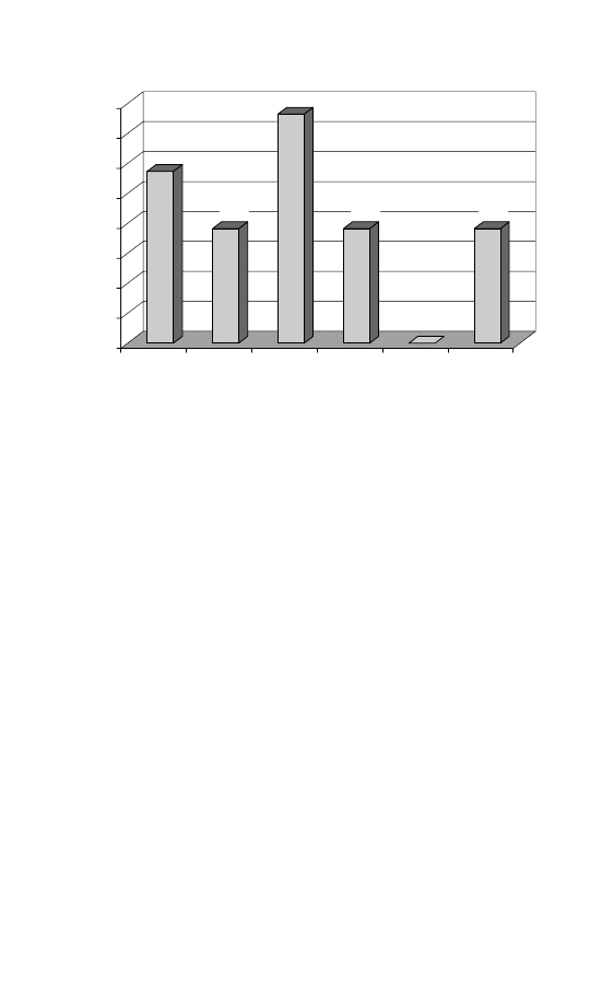
36
The Politics of Income Inequality in the United States
0.6%
0.8%
0.0%
0.0
0.1
0.2
0.3
0.4
0.5
0.6
0.7
0.8
SSI Public
assistance
Medicaid Educational
assistance
Housing
subsidy
Food
stamps
Percent reduction in inequality
0.4%
0.4%
0.4%
figure 2.6. Equalizing Effect of Means-Tested Government Benefit Programs
benefit. Only those below a certain income threshold (determined by
administering state agencies) can receive health care through Medicaid.
The same is true for all means-tested programs.
The equalizing effects of these means-tested benefits are charted in
Figure 2.6. This chart shows how much the Gini coefficient is reduced
when benefits from each program are included in income as opposed
to excluded from income. Of means-tested benefits, the largest equal-
izing effect is produced by Medicaid, but its 0.8 percent reduction in
inequality is still small in comparison to the effects of Social Security
and Medicare. The next largest effect is that of the SSI program. The
public assistance programs that are so often at the center of political
dialogue come next (public assistance and food stamps), but are only
about half as large as Medicaid in their impact.
The Total Government Contribution to Equality in 2000
Now we have seen the distributional consequences of several individ-
ual government programs, from the income tax to welfare assistance.
When the distribution of income excluding all government income
sources is compared to the distribution including these sources one
at a time, it becomes clear that nearly all government programs that

The Distributional Force of Government
37
table 2.2. Distribution and Level of Income by Deciles in
the United States, 2000
Pre-Redistribution Income
Post Government Income
Deciles
Share (%)
Mean
Share (%)
Mean
1
0
$0
2
$10, 988
2
1
$5, 323
3
$16, 835
3
3
$15, 225
4
$22, 182
4
4
$24, 798
6
$28, 226
5
6
$34, 483
7
$34, 281
6
8
$45, 363
8
$42, 339
7
10
$58, 076
10
$51, 982
8
13
$73, 790
13
$63, 710
9
18
$96, 995
16
$80, 460
10
36
$200, 605
31
$156, 855
explicitly take or give money to individuals equalize incomes.
10
The
issue I turn to in this section is the tangible effect of government
programs considered collectively.
I begin by comparing the distribution of income by deciles in
Table 2.2. I use deciles in this case because they yield some insights that
could not be seen in income shares by quintile. The first two columns
show the income shares and levels of each income decile based on the
now familiar concept of pre-redistribution income. The columns on
the right of the table show the same information for a different income
concept – post-government income. Post-government income accounts
for the effects of taxes and government benefit programs by subtract-
ing federal taxes from and adding the value of government benefits to
pre-redistribution income.
The data in this table tell an interesting story. First of all, without
government benefits, the bottom 10 percent of households would have
essentially no income. These households consist primarily of elderly
10
It is certainly not the case that every government policy, even redistributive policy,
benefits the poor. There are some high-income individuals who receive Social Security
benefits. Subsidies to higher education often directly benefit middle and upper income
individuals more than the poor. Certain tax programs undoubtedly benefit the rich
more than the poor (Johnston 2007). Despite this, to the extent that the impact
of government programs can be measured with income data, the overall impact of
government provides more benefits to the less well-off than the richest Americans.

38
The Politics of Income Inequality in the United States
individuals who do not work and have no private pension or retire-
ment income. Without the government these individuals would have
no money for food, shelter, or basic health care. The second decile is
not much better off, with only a 1 percent share of aggregate income
and an average of a little over $5,000 available for basic expenses.
Those in the third and fourth income deciles have an average of over
$15,000 from nongovernment income sources – enough to provide a
basic standard of living in the United States, but by no means a luxu-
rious existence. At the other end of the income distribution, however,
households are very well-to-do prior to government action. The top
10 percent of households garnered approximately 36 percent of pre-
redistribution income in 2000, providing an average household income
of over $200,000.
The distribution of post-government income is quite different. The
two right columns of Table 2.2 show that households at the bottom
of the income distribution, while not getting rich by any means, are
more likely able to subsist on government benefits. The bottom decile
(of primarily retired persons) garnered a 2 percent share of aggregate
post-government income, with an average income of nearly $11,000.
The top of the income distribution is also substantially different, with
the income share of the top 10 percent reduced from 36 to 31 percent
by government programs and the average income of these households
reduced by a striking $44,000. This table also makes clear that the
lion’s share of redistribution is from the top 20 percent of households
to the bottom 40 percent. The income share of the middle 40 percent
of households remains essentially the same between pre-redistribution
and post-government income.
Figure 2.7 quantifies the reduction in inequality that is caused by
certain types of government programs – taxes, mean-tested benefits,
non-means-tested benefits (both including and excluding Social Secu-
rity and Medicare), all benefits combined, and the total effect of federal
taxes and benefits. This chart depicts an American welfare state that
is different from the one that is so often mythologized in political
debate. While distributional concerns are not often discussed openly
in American politics, they are most common in debates over taxes
and means-tested benefit programs. Democrats and Republicans have
pretty clear differences, for example, on how the tax burden should
be distributed, with those on the left continually pushing for more
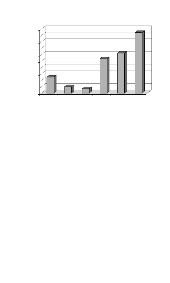
The Distributional Force of Government
39
5.0%
2.0%
1.3%
10.7%
12.4%
18.9%
0.0
2.0
4.0
6.0
8.0
10.0
12.0
14.0
16.0
18.0
20.0
Federal
taxes
Means-
tested
benefits
General
benefits
excluding
SS and
medicare
Including
SS and
medicare
Combined
benefits
Total
effect
Percent reduction in
inequality
figure 2.7. Combined Equalizing Effect of Government Action in the United
States, 2000
progressive forms of taxation. What we see in this chart, however,
is that taxes and means-tested benefits are not where the majority of
redistributive action is. Taxes and means-tested programs do have an
impact on income inequality, but taxes reduce inequality by only 5 per-
cent, and means-tested programs equalize incomes by only 2 percent.
This result probably should not be surprising. It would be difficult for
programs that take up such a small portion of federal expenditures to
make a massive difference in income inequality.
The more surprising result is for the effect of general benefit pro-
grams that are not specifically designed in such a way as to target the
poor. Income inequality is not usually mentioned explicitly in political
debate about these general benefit programs. Sometimes there are ques-
tions about whether benefits like Social Security and Medicare should
be made at least somewhat contingent on income, and questions about
the level of benefits that should be provided in these programs are also
common. It is clear, however, that most of government’s influence
on income inequality is achieved through such programs. Non-means-
tested benefits (excluding Social Security and Medicare) reduce income
inequality by only 1.3 percent, but Social Security and Medicare have

40
The Politics of Income Inequality in the United States
truly massive effects. When these two benefit programs are added, non-
means-tested programs reduce inequality by a staggering 10.7 percent.
In fact, more than 60 percent of government’s 18.9 percent reduction in
inequality through taxes and expenditures can be attributed to benefit
programs that are not specifically targeted to the poor.
It is interesting that perhaps the two most popular benefit programs
in the United States (Social Security and Medicare) are also the two
most redistributive. Take away the progressive income tax, welfare
of all kinds, unemployment compensation, disability, and on and on,
and you produce effects on the income structure of Americans smaller
than those produced by these two programs alone. For those on the
political left who are frustrated by the degree of conservative sentiment
in the United States, this information might be encouraging. Despite a
general lack of concern about equalizing economic outcomes, two of
the most sacred and untouchable programs in the United States are, in
fact, highly redistributive. This phenomenon is actually not unique to
the United States. In other more generous welfare states, many benefits
are not so highly contingent on income. Welfare state generosity is
politically feasible when government benefit programs are not about
rich versus poor, but when the programs are designed to extend useful
benefits to all citizens in society.
Given this, the two issues on the current American agenda that could
have the largest distributional impact in the future are health care and
Social Security. Making health care a guaranteed benefit would likely
have an equalizing effect – perhaps a large one. Contrarily, minimiz-
ing or eliminating guaranteed benefits through Social Security would
certainly have the opposite effect.
Market Conditioning
The programs that I have discussed to this point are probably the ones
that come to mind most often when thinking about the distributional
influence of government. Redistributional programs – those that explic-
itly take money from some through taxes and give to others via benefit
programs – have clear and obvious distributional effects. Entitlement
programs like Social Security and Medicare have the largest equaliz-
ing influence, but even when all explicitly redistributional programs
are taken together, they do not begin to account for all government

The Distributional Force of Government
41
activity. I argue here that many, if not most, other government activ-
ities have the potential to influence distributional outcomes as well.
Programs that are not explicitly redistributive can nonetheless influence
distributional outcomes via a mechanism I call market conditioning.
Market conditioning arises when government action produces eco-
nomic outcomes different than those which would be produced by
market forces in the absence of government action – that is, when
the state modifies or manipulates private market decisions. This is a
broad definition that encompasses a wide variety of government activ-
ity. Nearly everything government does, from basic regulation to any
form of taxation, influences markets at the margin. That market con-
ditioning occurs in general is obvious – any action that government
takes has an influence on society. The “market” outcomes that we
observe are not void of government influence, thus the scare quotes.
When 600,000 new jobs are created in a given quarter, that job growth
does not occur in a completely laizes-faire market system. Government
activities influence economic decisions made by a multitude of individ-
uals and firms, and some of these decisions are likely to influence the
labor market in which new jobs are created.
There is no doubt that market conditioning occurs. Government
activity unavoidably influences markets both directly and indirectly.
The question is whether market conditioning is truly a mechanism for
government influence on distributional outcomes. For market condi-
tioning to have an influence on distributional outcomes, at least some
policies void of explicitly redistributional goals must change market
processes in some way that produces differential benefits to those who
would be at the top or bottom of the income distribution without the
intervention of government.
11
While all policies have market condi-
tioning effects, this is not to say that all market conditioning actually
influences distributional outcomes. Some policies may influence mar-
kets in a way that has no real effect on income inequality. Furthermore,
some policies may condition markets in a way that increases inequality
while others might condition markets in an equalizing fashion. If these
11
These market conditionings could shift inequality either higher or lower. For inequal-
ity to be reduced, of course, market conditioning would have to benefit the poor more
than the rich. As Johnston (2007) points out in his journalistic account, there are
many government activities that explicitly redistribute toward the top of the income
distribution.

42
The Politics of Income Inequality in the United States
countervailing market conditioning forces simply cancel one another
out, then government would have no net impact on distributional
outcomes via market conditioning.
Distributional outcomes can be influenced via market conditioning
by any policy that affects how much income individuals receive in labor
and investment markets. For a real distributional impact, of course,
these income effects must be distributed unevenly across society. There
are two basic ways to influence income garnered through labor and
investment markets. The first is by influencing the characteristics of
individuals. If the labor market values intelligence, experience, skills,
and so on, then the fortunes of those without these characteristics
will improve if these characteristics can somehow be acquired with
government assistance. The second is by influencing the market itself.
If government takes action that induces demand for or supply of a
particular kind of worker or changes investment rules, distributional
consequences might be felt.
I will return in a later chapter to the question of whether the sum
total of government policy has a systematic impact on distributional
outcomes via market conditioning. In this chapter, my goal is simply
to demonstrate that a wide array of government policies have the
potential to influence income inequality via a market conditioning
mechanism. In fact, some programs that do not explicitly redistribute
income nevertheless have obvious distributional consequences. Nearly
any governmental influence on market outcomes has the potential to
influence income inequality, but a few specific examples are useful for
illustrative purposes.
Education and Workforce Development
The clearest example of policies that influence the characteristics of
individuals in a way that would have likely distributional consequences
is public education and training programs. To conceive of the distri-
butional impact of public education, we must first imagine a world in
which public education does not exist. In this hypothetical world, peo-
ple would obtain formal education only if they could pay for it or find
a private entity willing to provide it to them. Needless to say, those
with economic means would find it much easier to obtain education
than those with little in the way of financial resources. This is the real
situation in some countries today and was more closely approximated

The Distributional Force of Government
43
early in U.S. history. The bottom line is that, to the extent employers
and other actors in the labor market value the skills produced by for-
mal education, those able to obtain it will be more likely to get ahead
economically than those without it.
With the public provision and funding of education, however, the
situation changes markedly. Rather than leaving people to fend for
themselves, public education provides the means for those at both the
top and the bottom to gain basic and valuable skills. Even with public
education, of course, some obtain more or better education than others,
and not all of these educational differentials are rooted in divergent
preferences.
12
Some who would like to obtain more education may
not be able to, but publicly providing a basic level of education levels
the playing field with regard to economic opportunity. It is, of course,
important to note that even if everyone received the exact same amount
of education, there would likely still be many differences that would
produce unequal outcomes. But educational attainment would not be
one of these differentiating factors.
Whether and how much public education is provided has obvious
distributional consequences. In a hypothetical society where high levels
of public education are available and no one is inhibited from educa-
tional achievement based on preexisting economic means, economic
outcomes are likely to be more equal than in an alternative society in
which education must be purchased like any other private service.
The difference between a society with no public education system
and a society like the contemporary United States with an extensive
system of public education is stark in terms of the expected distribu-
tional outcomes. Real political decisions, however, are not typically
about whether or not to have public education, but about how much
should be provided and what portion of the cost should be borne by the
public. It is no longer a matter of serious political debate, for example,
whether elementary education should be provided by the public. The
structure and existence of funding for higher education, on the other
hand, is often the subject of political disagreement. At this point in time,
12
Oftentimes, for example, funding levels for education in poor areas are much lower
than in more affluent areas. While there is debate about the degree to which fund-
ing translates into student performance, funding inequities are often present even
in public programs that provides important benefits to middle and lower income
families.

44
The Politics of Income Inequality in the United States
government is committed to the provision of primary and secondary
education but takes only limited action in the form of programs like
Pell Grants and student loan programs to provide education beyond
high school.
Given that this book is about the influence of national policy on
income inequality, public education might seem a strange choice as an
example because it remains true that the lion’s share of policy decisions
regarding public education occur at the state and local level. There are,
however, a variety of public education programs and policies under-
taken at the national level. The No Child Left Behind initiative is a
recent example of a national effort to level the educational playing
field. If the ostensible goal of this legislation is achieved, gaps in educa-
tional outcomes across geography, economic circumstance, race, and
ethnicity will be reduced. If this occurs, it should have implications for
future distributional outcomes. Importantly, the heart of the potential
redistributional effect is not in the form of direct payments to indi-
viduals or households. The effect comes through building skills and
knowledge that will be valued in the marketplace, with the idea being
that those who would otherwise not be valued by the market when
they seek employment will be valued because of the implementation of
NCLB.
Modifying the future marketability of today’s fifth graders can
clearly only condition future market outcomes. NCLB might also have
current market conditioning effects via its impact on companies that
provide educational testing services. The fact that standardized testing
is one of many requirements in the NCLB legislation means that compa-
nies providing related services stand to benefit. It is interesting to note
on this point that President George W. Bush’s younger brother, Neil,
began a company in 1999 that sells software designed to improve stu-
dent performance on standardized testing. This is market conditioning
– with somewhat opaque distributional consequences.
When it comes to illustrating the distributional effects of national
education policy, an even more tangible example is useful – the Pell
Grant program. Pell Grants are available to low income individuals to
use for expenses related to higher education. A portion of the distribu-
tional effect of Pell Grants comes via explicit redistribution. Individuals
receive money that they can use for educational expenses, and this
program is funded through general tax revenue. This is the explicitly

The Distributional Force of Government
45
redistributional aspect of the program. But Pell Grants also open the
door of opportunity to thousands of students each year. Without this
program, some students currently receiving a college education would
doubtlessly be unable to pay for college. In some cases, this might sim-
ply mean going to a more affordable institution, but for others it would
mean missing out on a college education altogether.
The redistributional effects of Pell Grants are immediate and obvi-
ous, and were in fact accounted for in the previous section under the
category of educational assistance. If I were to account for the explic-
itly redistributional effect of Pell Grants treated separately, the effect
would be small. The program simply is not large enough in terms of
expenditures to have a massive impact on the distribution of income.
But there are additional distributional consequences of this program
via market conditioning. The effect through this mechanism is not
immediate, but occurs over a longer time frame. Access to education
via Pell Grants will enable current students to earn more – much more
– in the labor market in the years to come.
The Pell Grant program illustrates two important points. First,
programs like this that aim to promote education and workforce devel-
opment (or any form of skill development) have potential distributional
implications because they provide participants with marketable skills
that will have a return in increased income at some point in the future.
Second, explicitly redistributional programs like Pell Grants often have
secondary effects that occur via the market conditioning mechanism.
Medicare, as another example, redistributes from rich to poor. This is
the direct effect of the program. But it indirectly influences the incomes
of doctors and health care providers by inducing demand (and pay-
ments) for services that many poor, elderly persons would not seek or
pay for otherwise.
13
Regulatory Policy
Regulations enforced by the Securities and Exchange Commission,
Environmental Protection Agency, Food and Drug Administration, or
13
One could argue that the reimbursement levels for Medicare participants is relatively
low. Regardless, many of these patients would produce absolutely no economic return
for health service providers were it not for government programs such as these. On
the other hand, Medicare reimbursement rates also have consequences for the price
of procedures performed outside of the Medicare system.

46
The Politics of Income Inequality in the United States
any other regulatory agency of the federal government are aimed at
producing different outcomes than would be produced by a completely
free and unregulated market. Some of these regulatory policies could
have distributional effects.
One regulatory issue that has received some attention in the media
is the expensing of stock options. For many years, companies were
permitted to provide their employees with stock options at no charge
to their profit/loss statements. In essence, corporations could provide
stock (that could be sold by the employee at some time in the future)
without having any current effect on their balance sheet. This strategy
was useful for a variety of reasons. First, providing stock to high-level
managers provided a strong incentive for these executives to keep the
company on course over the long-haul by tying their economic well-
being to that of the company’s stock price. Second, it provided start-up
companies, especially tech firms, with a low-cost tool to attract talented
employees. These firms might not be able to pay a great deal in current
salary, but they could provide the opportunity for future riches if the
company succeeded.
While stock options are not completely costless to a company, in
that there are future costs to a company issuing these options, the
immediate costs are much less than expanding payrolls. This was the
case, at least, until a recent regulatory decision that now requires the
expensing of stock options – that is, subtracting a current valuation of
stock options from current profit statements. Such a regulatory change
may have the future impact of lessening income inequality by limiting
the often massive income supplements that come to employees when
they exercise stock options.
A multitude of other regulatory policies have important economic
implications that could influence inequality and, at the very least,
change the relative standing of employees and business owners situated
in certain segments of the economy. A new environmental initiative,
for example, to allow logging in certain previously protected areas will
doubtlessly have an effect on logging corporations and their employees.
Whether such initiatives would increase or decrease income inequality
has no clear answer, but the economic well-being of loggers will likely
be enhanced.
The post-9/11 emphasis on security also provides a good exam-
ple of market conditioning, and homeland security initiatives have

The Distributional Force of Government
47
already provided a boon to security firms and industries providing
security-related goods and services. Entirely new companies have
sprung up marketing new technologies to increase homeland security.
Small companies have increased revenue by marketing products to law
enforcement. Salient Stills’, which is a video-enhancement provider,
began as a spin-off from the Massachusetts Institute of Technology
Media Lab marketing its VideoFOCUS product to media outlets seek-
ing to enhance images for publication. The company currently markets
its product as a tool for law enforcement, security, military, and intelli-
gence, significantly expanding its market beyond media providers such
as newspapers and internet sites. Of course the new focus on security
has spawned millions of dollars in new contracts for traditional defense
contractors as well.
Social Policy
Social policies also produce outcomes that diverge from those of a
hypothetical free market. Though the regulation of abortion is not
often discussed in distributional terms, it is likely a mistake to remove
distributional issues from the discussion completely. Abortion policy
has no explicitly redistributive component (except to the extent that
governments provide funding for abortions to low-income women,
which does not happen in the United States at the national level). But
it is not void of potential distributional consequences.
The availability of abortion may well have an equalizing influence
in the economic realm. A pregnancy is full of economic implications. It
certainly increases medical expenses in the short term and in the long
term if the fetus is brought to term and remains with the mother after
birth. But expenses are not of any concern when the emphasis is on
income inequality. A pregnancy has income implications as well. In the
short term, giving birth almost always requires time away from work.
In the long term, again if the fetus is brought to term and raised by the
parent(s), having a child forces some into difficult economic choices.
How many hours can I work and still be a good parent? How much
time can I reasonably expect to take off from work to deal with child
care, doctors’ visits, and other aspects of raising a child? The stakes of
these questions become particularly important for those at the bottom
of the income distribution.

48
The Politics of Income Inequality in the United States
Imagine a single, 20-year-old woman who is pregnant with her first
child. Perhaps she is attending college and has a seemingly bright eco-
nomic future. How would having the child influence her? She might not
be able to complete college. This in and of itself hurts her prospects for
future economic prosperity. After having the child she has to find work,
but childcare is expensive and it may be hard to find a job with the kind
of flexibility that is so often needed by someone raising a child on her
own. Of course this is an extreme example. At least some women in this
situation would have support from family or friends that could allevi-
ate some of these problems, but the bottom line is that an unplanned
pregnancy has the potential to derail future economic prospects. While
adoption would be an (often complicated) option regardless of abor-
tion policy, permitting the termination of this woman’s pregnancy also
alleviates threats to a bright economic future. Restricting abortion has
economic consequences for pregnant women, and it is an impact that
would likely be felt most strongly by low-income single women with
few social support structures.
14
conclusion
This chapter has discussed two mechanisms through which government
can influence distributional outcomes – explicit redistribution and mar-
ket conditioning. Explicit redistribution is the mechanism that is most
commonly considered as an influence on distributional outcomes. In
the first part of the chapter, I described several redistributional pro-
grams and showed their substantive impact on income inequality in
the year 2000. When we focus on explicit redistribution, the programs
that matter most are not welfare programs targeted toward the poor.
The programs that redistribute the most are those that could best be
described not as redistributive welfare programs but as general social
insurance provision – Medicare and Social Security. The reason these
programs redistribute so much is that they are large programs targeted
toward the elderly – a demographic group that earns little in the market
due to their age.
14
This is by no means meant as a defense of abortion, which is a complicated ethical and
moral issue. The only point is that even a policy such as abortion, that on its face has
nothing to do with redistribution, can nevertheless have distributional consequences.

The Distributional Force of Government
49
The market conditioning mechanism, however, receives much less
attention as a mechanism for distributional impact. I argued that every-
thing government does has a direct or indirect effect on the economy.
The economic outcomes that are produced by the market are only
in part produced by free market forces and in part induced by gov-
ernmental action. If government did not exist, nearly every economic
interaction that we observe would likely be different and produce dif-
ferent outcomes. The level of economic inequality that we observe
prior to the effects of taxes and transfers is essentially government
conditioned market inequality.
The real question in the context of this book is whether these mar-
ket conditionings that occur whenever government takes action of any
kind actually produce a systematic influence on distributional out-
comes. I began to answer this question by briefly discussing a few
areas of policy that are not explicitly redistributive but have likely
consequences for the current or future distribution of income. Policies
designed to enhance the workforce influence the characteristics of indi-
viduals in such a way as to increase their value in the labor market.
These policies also affect the supply of skilled laborers. Regulatory poli-
cies advantage some industries over others and almost certainly have
marginal effects on any person connected with the affected industry.
Finally, even social policies like abortion can be construed to influence
distributional outcomes.
The discussion in this chapter just begins to scratch the surface.
I have by no means conducted an exhaustive discussion of every govern-
ment policy that might influence income inequality.
15
To the contrary,
my goal in this chapter was simply to demonstrate that policies that
do not explicitly redistribute income could influence income inequality
via other mechanisms.
Notably missing from this chapter is any quantification of the distri-
butional impact of these market conditioning policies. This is because
the marginal effects of such policies are impossible to capture because
we do not know how the world would look in the absence of all gov-
ernment action. This would be the baseline for comparison needed to
quantify effects, but it is not observable. An additional issue is that the
15
Page and Simmons (2000) discuss a variety of programs such as these in much greater
detail.

50
The Politics of Income Inequality in the United States
distributional effects of many of the market conditioning programs
are so marginal that it would be hard to parse out the influence of
an individual program or policy. I return in Chapters 4 and 5 to the
question of whether market conditioning has a systematic influence on
income inequality. In the next chapter, I discuss some of the basic
political divisions surrounding income inequality, distribution, and
redistribution in U.S. national politics. What government does influ-
ences distributional outcomes, but how is the battle over “who gets
what” structured? This will take us one step closer to answering the
question of how political and distributional dynamics are linked.

3
Political Conflict over “Who Gets What?”
When we examine a cross-section of income data, as in the previous
chapter, it is obvious that government programs have a tangible impact
on who has how much money in America. Government action mat-
ters, but I am most interested in the political conflict that produces
this government action. Government’s impact on inequality, occur-
ring through a variety of policy mechanisms, does not just happen,
appearing out of nothing. It is likely a systematic product of politics. If
we think of politics as the conflict over which values government will
authoritatively enforce or the battle over who gets what, it is obvious
that who wins and who loses in political conflict should alter the distri-
butional outcomes that are in part determined by government policy.
In this chapter, I examine the nature of political conflict over distribu-
tional outcomes in the United States. How might politics, as opposed
to programs, influence income inequality?
Since at least the time of FDR and the Great Depression, modern
American liberals have placed an intrinsic value on economic equality
and have generally favored government action to balance the scales
between the rich and the poor. Conservatives, on the other hand,
do not find economic inequality to be an inherent societal problem
and are less favorable toward government action that balances the
scales of inequality. This is not to say that conservatives are uncon-
cerned with the plight of the poor or lack compassion toward those
less fortunate, but liberals are clearly more supportive of government
action to reduce inequality, while conservatives believe the free market
51

52
The Politics of Income Inequality in the United States
should determine distributional outcomes. The questions I address in
this chapter are how these theoretical ideological differences manifest
themselves in political decision making and whether ideological dis-
agreement extends beyond debate over explicit redistribution to the
more amorphous distributional consequences of market conditioning.
In order to shed light on these questions, I present two types of evi-
dence in this chapter. In the next section, I examine the debate over
the marriage “penalty” tax in some detail to flesh out how liberals and
conservatives, Democrats and Republicans, operationalize their theo-
retical differences on distributional questions – in this case, on an issue
in which popular accounts placed distributional concerns at the periph-
ery. While few should doubt that Republicans and Democrats differ
in their positions on issues of taxation, the marriage penalty debate is
an interesting case because it was not a general tax package with read-
ily apparent distributional implications. Nevertheless, distributional
concerns were inserted into the debate. After discussing the marriage
penalty tax, I turn to a more systematic examination of distributional
attitudes in the House of Representatives, utilizing evidence from a
survey of the 106th House conducted during the summer of 2004.
a case study in distributional debate: the marriage
tax “penalty”
The debate over the marriage tax “penalty” began to gather momen-
tum after the Republican takeover of Congress in 1994. The marriage
tax “penalty” refers to a situation in which two people pay more in
federal income taxes as married filers than they would if they were
unmarried individuals. Consider the following example, presented in
detail in first two columns of Table 3.1, which is based on tax law as
it existed in 2000. Joe and Mary both earn about $30,000 per year.
If Mary and Joe are not married, their individual tax liability would
be $3,420 each. If married, their joint tax liability would be $7,474
(both assuming standard deductions). Joe and Mary pay $634 less in
combined taxes as unmarried individuals than they would as a married
couple. This is a marriage tax “penalty.”
This shows one way in which tax law in 2000 (and for several
years before) violated the concept of marriage neutrality. The ideal of
marriage neutrality in a tax system is that two single individuals should

Political Conflict over “Who Gets What?”
53
table 3.1. Marriage Bias in the Federal Income Tax
Couple
1
Couple
2
Joe
Mary
Sam
Karen
As Individuals
Income
$30,000
$30,000
$60,000
$0
Personal Exemptions
$2,800
$2,800
$2,800
$2,800
Standard Deduction
$4,400
$4,400
$4,400
$4,400
Taxable Income
$22,800
$22,800
$52,800
$0
Tax Calculation
15% $0–$26,250
$3,420
$3,420
$3,938
$0
28% over $26,250
$0
$0
$7,434
$0
Total Tax
$3,420
$3,420
$11,372
$0
As a Couple
Income
$60,000
$60,000
Personal Exemptions
$5,600
$5,600
Standard Deduction
$7,350
$7,350
Taxable Income
$47,050
$47,050
Tax Calculation
15% $0–$43,850
$6,587
$6,587
28% over $43,850
$887
$887
Total Tax
$7,474
$7,474
Marriage Penalty (Bonus)
$634
($3,898)
Note: Calculations assume standard deduction and ignore effects of Earned
Income Credit.
pay no more or less in taxes if they become married. In other words, a
marriage-neutral tax system would have no economic influence on deci-
sions regarding marital status. I place the scare quotes around penalty
in the example above because the tax system as it existed in 2000
not only created penalties for some married couples, but also created
bonuses for others. Another example, in the third and fourth columns
of Table 3.1 will serve to illustrate the marriage “bonus.” Sam earns
$60,000 per year and Karen earns nothing. As an individual, obviously
Karen would have no tax liability. Sam, however, would owe the IRS
$11,372. If Sam were to marry Karen, however, their joint liability
would be only $7,474. This is a $3,898 gain to Sam for becoming mar-
ried. In this case the marital status bias is positive rather than negative.
In terms of statutory structure, there are literally dozens of pro-
visions in the federal income tax that generate bias toward marital

54
The Politics of Income Inequality in the United States
status, but the three largest contributors to marriage bias are the stan-
dard deduction, the width of tax brackets, and the phase-out rate of the
Earned Income Credit (EIC) for individuals vis-à-vis married couples
(General Accounting Office). Other contributing factors include the tax
treatment of Social Security income and the Alternative Minimum Tax.
The income split, or the proportion of family income that each
spouse earns, is the determining factor in whether or not marriage
bias in the tax code produces a bonus or penalty. Couples with an
even income split generally pay the largest penalties, while the largest
bonuses accrue to single-earner couples. For example, in 2000, the
standard deduction was $4,400 for an individual and $7,350 for joint
returns. One reason the couple with an even income split from above
(Joe and Mary) pays a marriage penalty is that they would be able to
deduct a total of $8,800 if filing as individuals. The penalty in this
case is created because the standard deduction for married couples is
not twice that for individuals. For the single-earner couple above (Sam
and Karen), however, there is a bonus because their deduction moves
from $4,400 to $7,350 with no change in their aggregate income. This
example is based on the standard deduction, but a similar set of results
is produced by the width of income tax brackets. When a tax bracket
is not twice as wide for a married couple as opposed to a single individ-
ual, single-earner couples will receive a bonus and those with a more
even income split will pay a penalty. This is the case because couples
with only one earner can claim two personal exemptions even if only
one spouse is earning.
So, a lack of marriage neutrality in the tax code clearly existed dur-
ing the 1990s. By virtue of being taxed as a unit, some couples paid a
marriage penalty and others received a bonus. During the mid-1990s
some Republican members of Congress began to argue for changes to
the tax code that would eliminate the marriage penalty (but not neces-
sarily the bonus).
1
A wide array of legislation was introduced aimed at
the marriage penalty. A few more details regarding how these marriage
penalties and bonuses came into existence will aid in understanding the
1
Interestingly, laws preventing gay and lesbian couples from wedding create a situation
in which they cannot suffer a marriage penalty or bonus. So, eliminating penalties and
maintaining bonuses shift the tax burden to unmarried individuals, including gays and
lesbians, some of whom would like to be married but are unable to legally do so.

Political Conflict over “Who Gets What?”
55
various proposals targeted at the marriage penalty that were considered
in the late 1990s and early 2000s.
A Brief History of Marriage Bias in the Federal Income Tax
One way to discuss the history of federal income tax law as it relates to
marriage bias is to focus on three forms of equity – marriage neutral-
ity, progressivity, and equal taxation of couples with equal earnings.
Marriage neutrality, as discussed above, means that a couple will pay
no more or less in aggregate taxes as a couple than they do as indi-
viduals. Progressivity refers to the idea that those with higher incomes
should be taxed at a higher rate than those with lower incomes. Equal
taxation of couples simply means that married couples with the same
amount of money should pay the same amount in taxes. As we will
see, these goals cannot all be achieved at the same time.
A 2001 Congressional Research Service Report utilizes an exam-
ple that illustrates the tension between these three goals quite well
(Esenwein 2001). We can go back to our four individuals from
Table 3.1: Joe ($30,000 income), Mary ($30,000 income), Karen (no
income), and Sam ($60,000 income). If these four were treated strictly
as individuals, then progressivity would dictate that Joe and Mary
earning $30,000 would each be taxed at a lower rate than Sam earn-
ing $60,000. Marriage neutrality dictates that if Mary and Joe become
married and Sam and Karen also get married, each couple’s combined
tax liability would remain the same as it did when unmarried. But the
third goal, equal taxation of couples with the same amount of income,
dictates that both couples should pay the same amount of tax on their
$60,000 of combined income. This would create a situation in which
Sam is paying tax at the same rate as both Joe and Mary, and this runs
counter to the ideal of progressivity. The CRS report summarizes the
situation as follows:
Regardless of how these three concepts of equity are juggled, under current
definitions an income tax can be designed to achieve any two of these goals,
but it cannot achieve all three. The system might be marriage-neutral and tax
couples with equal incomes equally but it could not be progressive. As an
alternative, the tax system might be progressive and tax couples with equal
incomes equally but then it would not be marriage-neutral. Finally, the tax

56
The Politics of Income Inequality in the United States
system could be progressive and marriage-neutral but not tax couples with
equal incomes equally (Esenwein 2001).
The balancing of these three goals in the U.S. federal income tax
has not been constant over time. When first implemented in 1913, the
federal income tax required each individual to file separately. That is,
married couples filed as two individuals. Divergent property laws in
different states, however, created advantages for some couples under
this system. Specifically, married couples from common law states were
required to treat their incomes separately. Couples in states with com-
munity property laws, however, could divide their income between
the two spouses. In community property states, then, a couple could
reduce their total tax liability by evenly splitting their income and thus
subjecting the higher-earning spouse’s wages to a lower marginal rate.
In terms of the three forms of equity, this system was marriage-neutral
and progressive (at least in common law states) but did not tax couples
with equal earnings equally (Esenwein 2001).
The Revenue Act of 1948 created the basic structure of the tax sys-
tem currently in place. In an effort to insure equal taxation of couples
residing in different states with the same amount of income divided
between spouses in the same way, Congress modified the tax code
to create different tax rate schedules for singles and married couples.
Deductions were larger and the tax brackets were wider for married
couples than for singles so that, regardless of whether a couple was
in a common law or community property state, they would pay the
same amount of federal income tax. While this change in the tax code
created equal taxation of couples with equal incomes, it introduced
marriage bias into the tax structure. Many individuals (depending on
the income level of their prospective spouse) could reduce their tax lia-
bility by getting married. So, the Revenue Act of 1948 created the first
marriage bonus in the federal income tax.
For single individuals, however, this change could just as easily be
called a singles penalty as a marriage bonus. Many people thought it
unfair that a single woman paid more in taxes than a married man
earning the same amount. Vivien Kellens, on behalf of the War Wid-
ows of America, testified before the Ways and Means Committee in the
late 1960s that she unfairly paid a penalty due to the lack of suitable
men created by deaths in World War II. This, in part, led to the 1969

Political Conflict over “Who Gets What?”
57
Tax Reform Act. This modification of tax law aimed to ensure that
no single individual would pay in excess of 20 percent more in taxes
than a married couple with the same income. This was accomplished
by widening tax brackets for individuals. It also meant, however, that
some married couples paid more as a couple than they would as sep-
arate individuals. This was the first marriage penalty. Thus, the Tax
Reform Act of 1969 did not really reduce marriage bias as much as it
shifted the bias to fall more on married couples than before the reform.
Two important changes in the income tax occurred during the 1980s
– one set of changes resulted from the Economic Recovery Act of
1981 and the other resulted from the massive tax code overall in
1986. Both of these changes had implications for marriage neutral-
ity. Armed with the knowledge that only couples with two earners
paid marriage penalties, the Economic Recovery Act of 1981 included
a deduction for married couples equal to 10 percent of the lower earn-
ing spouse’s income, not to exceed $2,000. While this did eliminate the
penalty for some (but not all) couples, it also increased the bonus for
other couples. This change also reintroduced the problem of not tax-
ing couples with equal earnings equally because a single-earner couple
would owe more in taxes than a dual income couple with the same
income. The 1986 Tax Reform Act had implications for marriage
neutrality indirectly, via a major change in progressivity. Reducing
fourteen tax brackets to two and increasing the standard deduction
for joint returns more than for individual returns reduced progressiv-
ity and the marriage bias. A variety of other provisions in this major
tax overhaul also influenced marriage neutrality. With the 1986 Act,
the two-earner deduction created in 1981 was repealed, contributions
limits to Independent Retirement Accounts were different for married
couples and individuals, and new deductions for the elderly and the
blind were a function of marital status. So, the Tax Reform Act of
1986 increased marriage neutrality through reductions in progressiv-
ity, but also increased marriage bias through a variety of provisions
dependent on marital status.
Changes in the early 1990s moved the structure of the income
tax toward its pre-1986 form. After the Omnibus Budget Reconcili-
ation Act of 1993, the tax code returned to five brackets and greatly
expanded the Earned Income Credit, thus increasing structural progres-
sivity at the expense of marriage neutrality. So, it was in this context –

58
The Politics of Income Inequality in the United States
some couples paying marriage penalties and others receiving bonuses
– that the Republicans took over Congress after the 1994 mid-term
elections. One of their targets was the marriage penalty. Over the next
several years, proposals to eliminate marriage penalties were repeatedly
offered, and partisan differences over this issue demonstrated divergent
perspectives on government’s role in distribution and redistribution.
Targeting the Marriage Penalty in the Post-Republican
Revolution Congress
After the Republican takeover of Congress beginning with the 104th
Congress convening in 1995, efforts to eliminate the marriage tax
penalty began to gain momentum. Still, while some Republican mem-
bers of Congress had been proposing legislation targeted at reducing or
eliminating the marriage penalty for several years, tax relief for married
couples was not the most immediate priority to Republican leaders in
the House and Senate. The first successful efforts to provide substantial
tax relief to married couples came during the 106th Congress when the
Marriage Penalty Tax Relief Reconciliation Act of 2000 (H.R. 4810)
was passed by both the House and Senate. President Clinton, how-
ever, vetoed this measure. After the election of George W. Bush, the
Congress again took action on tax relief for married couples, and this
relief became law when President Bush signed the Economic Growth
and Tax Relief Reconciliation Act of 2001. I will focus on the 2000
debate because it was focused specifically on the marriage penalty,
whereas the 2001 debate was more general due to the fact that it was
motivated by the broad tax cuts proposed by George W. Bush.
The marriage penalty tax would not seem at first blush to have
a great deal to do with distributional outcomes. Of course any tax
legislation has the potential to change distributional outcomes, but
marriage bias in the federal income tax does not seem to naturally pit
the rich against the poor. This, in fact, is one of the reasons I have
chosen to present the marriage penalty tax as a case study – it is not
a natural case for distributional debate. As we will see, however, even
this debate brought disagreements about distribution and redistribu-
tion into focus. Examining the debate that occurred surrounding these
legislative efforts to reduce the marriage penalty provides insight into
partisan differences on distributional questions.

Political Conflict over “Who Gets What?”
59
The Marriage Tax Debate in 2000
Various strategies were proposed to deal with the marriage penalty,
ranging from providing special deductions for two-earner families, to
increasing the phase-out point of the Earned Income Credit for married
couples, to widening tax brackets and increasing standard deductions,
to making single filing optional. Notably absent from any of the legisla-
tive proposals were tax code changes that would have achieved mar-
riage neutrality. Most of the proposals only partially eliminated mar-
riage penalties, kept marriage bonuses intact, and actually increased
the tax rates of unmarried individuals relative to married couples.
While dozens of bills aimed at the marriage penalty were intro-
duced, in the end the debate came down to one strategy presented by
the Republicans and two alternatives presented by the Democrats. The
basic strategy of the Republican proposal (H.R. 4810, S. 2839) was to
increase the phase-out point of the Earned Income Credit for married
couples, increase the standard deduction for couples to twice that for
singles, and widen the 15 percent tax bracket for married couples to
twice that of singles.
2
The House Democratic alternative (H. AMDT.
571) was similar to the Republican proposal except that it did not
widen the 15% tax bracket and made the implementation of the tax
cut contingent on Social Security and Medicare trust fund surpluses
as well as national debt projections. Senate Democrats in 2000 pre-
sented optional single filing as a way to completely eliminate marriage
penalties, but this option was to be phased out for couples with over
$100,000 in taxable income (S. AMDT. 3863).
Before taking a more detailed look at the rhetoric surrounding this
issue, it is useful to understand the real distributional implications of
the plans. The clearest way to compare the main Republican and Demo-
cratic alternatives is to examine how much couples at various points
in the income distribution benefit from the tax reductions. Table 3.2
clearly shows that the House Democratic plan favored those at the
middle and bottom of the income distribution much more than the
Republican plan. This is due to the fact that the Republican plan
included widening of the 15 percent bracket and the Democratic plan
did not. Widening even the lowest tax bracket provides the greatest
2
This is the same basic strategy that eventually became law in 2001.

60
The Politics of Income Inequality in the United States
table 3.2. Tax Cuts (in $billions) to Married Couples at Specified
Levels of Taxable Income
House GOP
House Dem
Income
Deduction
and EIC
Bracket
Widening
Benefits
(%)
Deduction
and EIC
Benefits
(%)
<$10K
$0.0
$0.0
0.1
$0.0
0.3
$10–20K
$0.5
$0.0
2.0
$0.6
8.8
$20–30K
$1.2
$0.0
5.0
$1.4
20.9
$30–40K
$1.0
$0.0
4.1
$1.1
16.3
$40–50K
$0.9
$0.0
3.8
$0.9
14.3
$50–75K
$1.6
$2.9
18.5
$1.6
25.2
$75–100K
$0.6
$6.6
29.4
$0.6
9.4
$100–200K
$0.3
$6.7
28.5
$0.3
4.0
>$200K
$0.1
$2.1
8.6
$0.1
0.9
Source: Center for Tax Justice.
absolute benefits to those with moderately high incomes because this
widening is identical to a marginal tax rate cut for those previously in
the second (28 percent) tax bracket or higher. The differences between
the Senate Republican and Democratic plans (data not shown) are even
more clearly distributional in nature because the initial Republican
proposal by Senator Roth (DE) widened not only the 15 percent tax
bracket but also the 28 percent bracket, while the Senate Democrats’
alternative explicitly made marriage penalty reductions contingent on
income levels.
The basic argument of Republicans was an appeal to fairness and
equity in the tax system – two individuals should not have to pay
higher taxes as a married couple. Congressman Jerry Weller (IL) clearly
articulated the Republican position in a floor statement on July 12,
2000 (Congressional Record H5859-60):
We have often asked in the House Chambers, many of us, is it right, is it fair
that under our Tax Code 25 million married working couples, on average, pay
almost $1,400 more in higher taxes just because they are married. Now, is
that right, is that fair, that if a couple chooses to participate in the most basic
institution in our society, marriage, that they are going to pay higher taxes
if they work? Unfortunately, under our Tax Code, that is true. If a husband
and wife are both in the workforce, both the man and the woman are in the

Political Conflict over “Who Gets What?”
61
workforce, a two-income household, under our Tax Code they will file jointly
and, because of that, they will pay a marriage tax penalty. That is just wrong.
We have made this a priority, to eliminate the marriage tax penalty suffered
by 25 million married working couples.
While the Democrats agreed in principle with reducing marriage
penalties, they objected to the Republican strategy for three primary
reasons. First, the Republican plan provided tax cuts to couples even
if they were paying no tax penalty. Second, the size of the tax cut
decreased revenue to an alarming degree in the eyes of Democrats.
Finally, they had distributional concerns that are fairly obvious from
the table presented above. These concerns were summarized by Con-
gressman Sander Levin (MI) on the same day during the debate of H.R.
4810 (Congressional Record H5860):
I favor a marriage penalty tax relief bill. That is why I say to my colleague
on the Committee on Ways and Means, I am for the Democratic substitute,
and I can face the thousands of voters in my district, whose numbers the
Republicans like to cite for each of us in the House. We know our districts,
and I know this bill that I am supporting; the Democratic substitute is the
answer.
. . . First of all, half of the relief in their bill goes to those who do
not pay a marriage penalty. So they attach the marriage penalty label, though
more than half of the money does not apply to that situation. Secondly, many
families with kids will not get the full relief that the bill promises because of the
way they have shaped it. Thirdly, the lion’s share, and this is important, of the
money goes to the top quarter of the tax filers. Fourthly, look at the out-year
projections. Assuming the AMT is eventually applied, and the chairman of the
committee has promised that, the 20-year cost of their bill is $700 billion. That
plays lightly with the future of my grandchildren and with the need to address
Medicare and Social Security.
House Republicans were quick to point out, however, that the
Democratic alternative not only failed to provide as much general
tax relief as the Republican plan but also did less to reduce marriage
penalties. While neither plan presented in the House was designed to
fully eliminate marriage penalties, the fact that the Republican plan
did more was incontrovertible. In the end, the Democratic alternative
(H. AMDT. 571) was defeated 198 to 228, with just eight Democrats
joining Republicans (Roll No. 390). H.R. 4810 eventually passed the
House 269 to 159, with some bipartisan support for the final bill

62
The Politics of Income Inequality in the United States
(Roll No. 392). Clearly, however, the key vote on this piece of leg-
islation was that on the Democratic alternative, and it was nearly a
party-line vote.
Upon passage in the House, H.R. 4810 was taken up for considera-
tion in the Senate, and the first action was the complete replacement of
H.R. 4810 with an alternative (S. 2839) crafted by the Senate Finance
Committee chaired by William Roth (R-DE). The Senate Republicans
wanted to go even farther than the House version of the bill by not
only widening the 15 percent tax bracket but also widening the 28
percent bracket for married couples. The Senate Republican proposal
was designed to eliminate the marriage penalty for more couples and
expand tax relief more generally for those not subject to marriage
penalties. This proposal also meant that a greater proportion of tax
relief would be given to couples at the top part of the income distribu-
tion and this plan generated more lost revenue than the plan passed in
the House. Both of these factors raised the ire of Senate Democrats.
Unlike the House Democratic alternative, which was more con-
strained in its marriage penalty relief than the House Republican plan,
the Democratic alternative in the Senate promised to completely elim-
inate the marriage penalty for most households. The essence of the
Democratic plan in the Senate was optional single filing (S. AMDT.
3863). That is, couples could file either as individuals or as a married
couple. If they would be subject to a marriage penalty when filing as
a married couple, they could avoid the penalty by filing as two sin-
gle individuals. On the other hand, those couples already receiving a
marriage bonus could retain their bonus by continuing to file as a mar-
ried couple. However, the Democratic plan was designed to phase out
this single filing option as household adjusted gross income (AGI) rose
above $100,000, with the benefit completely eliminated for those with
AGI above $150,000.
Democrats argued that their strategy to reduce marriage penal-
ties was preferable to the Republican plan for three primary reasons.
First, the Democratic plan completely eliminated marriage penalties
for households with less than $100,000 in annual taxable income. The
Republican plan focused only on the largest culprits in the marriage
penalty: the Earned Income Credit phase-out, standard deductions, and
tax bracket width. Dozens of other provisions can create small marriage
penalties, and the Republican plan did nothing to address these issues.

Political Conflict over “Who Gets What?”
63
Second, the Democratic plan was less costly. This was the case because
the Democratic plan gave tax cuts only to couples paying a marriage
penalty while the Republican plan gave tax relief to couples regardless
of whether they were paying a penalty or receiving a bonus. The Demo-
cratic plan also saved money by targeting the tax cuts to approximately
the bottom 90 percent of households in the income distribution.
During the debate over the Republican and Democratic proposals,
several interesting exchanges took place on the floor of the Senate.
Senator Edward Kennedy (D-MA) made it clear that distributional
matters were central to the Democratic opposition of the Republican
proposal (Congressional Record S6792):
I want to be clear. I support legislation that would provide tax relief to the
working families who are currently paying a marriage penalty. Such a penalty
is unfair and should be eliminated. However, I do not support the proposal
which the Republicans have brought to the floor. While its sponsors claim the
purpose of the bill is to provide marriage penalty relief, that is not its real
purpose. In fact, only 42 percent of the tax benefits contained in the legislation
go to couples currently subject to a marriage penalty. The majority of the tax
benefits would actually go to couples who are already receiving a marriage
bonus, and to single taxpayers. As a result, the cost of the legislation is highly
inflated. It would cost $248 billion over the next ten years.
And, as with most Republican tax breaks, the overwhelming majority of the
tax benefits would go to the wealthiest taxpayers. This bill is designed to give
more than 78 percent of the total tax savings to the wealthiest 20 percent of
taxpayers. It is, in reality, the latest ploy in the Republican scheme to spend the
entire surplus on tax cuts which would disproportionately benefit the richest
taxpayers. That is not what the American people mean when they ask for relief
from the marriage penalty. With this bill, the Republicans have deliberately
distorted the legitimate concern of married couples for tax fairness
. . . .
. . . A plan that would eliminate the marriage penalty for married couples
could easily be designed at a much lower cost. The House Democrats offered
such a plan when they debated this issue in February. The Senate Democrats
are offering such an alternative plan today. If the real purpose of the legislation
is to eliminate the marriage penalty for those working families who actually
pay a penalty under current law, it can be accomplished at a reasonable cost.
The key to drafting an affordable plan to eliminate the marriage penalty is to
focus the tax relief on those couples who actually pay the penalty under current
law. The Republican proposal fails to do this, and, as a result, it actually perpet-
uates the marriage penalty despite the expenditure of $248 billion on new tax
cuts. Under the Democratic plan, the tax relief actually goes to those currently

64
The Politics of Income Inequality in the United States
paying a marriage penalty. It is also essential to target the tax benefits to the
middle income working families who need tax relief the most. The Democratic
plan focuses the tax benefits on those two earner families with incomes less
than $150,000. By contrast, major portions of the tax benefits in the Republi-
can plan would go to much wealthier taxpayers at the expense of those families
with more modest incomes. As a result, the Democratic proposal would cost
$11 billion a year less, when fully implemented, than the Republican plan, yet
provide more marriage penalty tax relief to middle income families.
The Republican response to these lines of argument brought the
marriage penalty tax debate squarely into the category of a classic
partisan debate over taxes. Republicans argued that their more costly
plan was appropriate because taxes should always be reduced in a
climate of budget surpluses. They also argued that marriage bonuses
are a misnomer and giving tax relief to single-earner couples not pay-
ing a marriage penalty is wholly appropriate. Finally, they argued that
targeting tax cuts away from the top of the income distribution is inap-
propriate. Senator Roth (R-DE) summarized the Republican argument
as follows (Congressional Record S6802, S7105):
According to the Congressional Budget Office, in 1999, there were about 7.5
million joint returns with an adjusted gross income greater than $100,000.
And 56 percent of that group, or 4.2 million couples, suffered from a marriage
penalty. The total amount of marriage penalty suffered by those couples is
almost $12 billion, which is more than one-third of all the marriage penalties
caused by our Tax Code.
The average marriage penalty faced by each one of these families is about
$2,800. Yet despite these significant marriage penalties encountered by these
couples – and they claim that this is a targeted tax bill to eliminate the marriage
tax – this substitute amendment [the Democratic alternative] turns its back on
those taxpayers. The amendment tells these folks they make too much money
and should not receive complete relief
. . . .
. . . I would ask those who oppose this family tax relief: Just how big will
America’s budget surplus have to get before America’s families deserve to
receive some of their tax dollars back? If not now, when? If eight percent
of just the overpayment is too big a refund, how little should it be? How long
do they have to wait? How hard do they have to work? How large an overpay-
ment do they have to make? This bill is fair. We have addressed the three largest
sources of marriage tax penalties in the tax code – the standard deduction, the
rate brackets, and the Earned Income Credit. And we have done so in a way
that does not create any new penalties – any new disincentives in the tax code.

Political Conflict over “Who Gets What?”
65
We have ensured that a family with one stay-at-home parent is not treated
worse for tax purposes than a family where both parents work outside the
home. This is an important principle because these are important families
. . . .
. . . Families across America are waiting for us to make good on our promise.
They are waiting for us to return some of this record surplus to them. Let’s
approve the Marriage Tax Relief Reconciliation Act of 2000 and let’s divorce
the marriage tax penalty from the tax code once and for all.
In the end, the Democratic plan was defeated on a nearly straight
party vote, with one Republican (Lincoln Chafee, RI) joining with
the Democrats (Record Vote 200). With the Democratic alternative
defeated, the Republican proposal then passed the Senate (Record Vote
215) with weak support from Democrats. There were, however, some
differences between the House and Senate version of the legislation
that had to be reconciled in conference. The main differences between
the two versions were that the Senate version expanded the 28 percent
bracket while the House bill expanded only the 15 percent bracket and
the Senate version phased in the tax cuts more quickly than the House
version. The conference agreement discarded the 28 percent bracket
expansion but phased the cuts in more quickly than the original House
version. The conference version of the legislation passed the House on
July 20, 2005 (Roll No. 418) and the Senate on July 27, 2005 (Record
Vote 226), both with moderate bipartisan support.
The legislation was forwarded to President Clinton, but the pres-
ident vetoed the legislation (by pocket veto), and in his remarks
explaining the veto, distributional concerns were again raised:
H.R. 4810 would cost more than $280 billion over 10 years if its provisions
were permanent, making it significantly more expensive than either of the bills
originally approved by the House and the Senate. It is poorly targeted toward
delivering marriage penalty relief – only about 40 percent of the cost of H.R.
4810 actually would reduce marriage penalties. It also provides little tax relief
to those families that need it most, while devoting a large fraction of its benefits
to families with higher incomes.
Taking into account H.R. 4810, the fiscally irresponsible tax cuts passed by
the House Ways and Means Committee this year provide about as much benefit
to the top one percent of Americans as to the bottom 80 percent combined.
Families in the top one percent get an average tax break of over $16,000, while
a middle-class family gets only $220 on average. But if interest rates went up
because of the congressional majority’s plan by even one-third of one percent,

66
The Politics of Income Inequality in the United States
then mortgage payments for a family with a $100,000 mortgage would go up
by $270, leaving them worse off than if they had no tax cut at all. We should
have tax cuts this year, but they should be the right ones, targeted to working
families to help our economy grow – not tax breaks that will help only a few
while putting our prosperity at risk.
The rhetoric on both sides of this debate was no doubt overheated,
with Republicans invoking images of middle-income couples toiling
under the weight of a government-imposed marriage penalty and
Democrats bemoaning an untargeted tax cut benefiting primarily the
wealthy. Given that upper income households pay a large proportion
of federal income taxes, it was somewhat misleading for Democrats
to label the Republican proposal as slanted toward the rich. Senator
Roth’s statement regarding the proportionality of tax cut benefits to
the aggregate taxes paid by income groups is well-taken. A tax cut that
benefits income groups in equal proportion to their tax burden will
inevitably benefit the rich more than the poor. The fact remains, how-
ever, that the Republican plan was more favorable to those at the upper
part of the income distribution than was the Democratic plan. Republi-
cans simply favored a more general tax cut than did the Democrats, and
this fact has distributional consequences that were a prevalent part of
the debate in both the House and the Senate. Eliminating the marriage
penalty does not inherently invoke distributional issues. Both the pol-
icy proposals and the rhetoric surrounding these proposals, however,
became intertwined with concerns about distributional consequences.
It seems clear from this perhaps somewhat unlikely example, then, that
determining who gets what is an important aspect of political conflict
in the United States.
systematic evidence of the partisan and ideological
divide over distributional outcomes
The debate over the marriage penalty provides a useful case study in
distributional disagreements between the major U.S. parties. The mar-
riage tax penalty was not, at the outset, an obvious distributional issue.
The marriage penalty did not fall on one income group to the exclu-
sion of others. But even in this case, the parties developed very different
strategies for reducing marriage penalties, with different distributional
implications. In this case, it is clear that Republicans were much more

Political Conflict over “Who Gets What?”
67
willing to extend the benefits of tax relief to those at the top of the
income distribution than were Democrats. While the marriage penalty
debate is a good illustrative example, it may not generalize to other
policy debates. Thus, in this section, I present some data evidencing
partisan and ideological divergence on more general distributional atti-
tudes. The goal of this section, like the last, is to show how Republicans
and Democrats and conservatives and liberals differ in their attitudes
about income distribution and what government can and should do
about it. But the evidence I present here is broader than that discussed
above. I analyze general attitudes rather than a specific policy proposal.
I focus on assessing the distributional preferences of Democratic
and Republican members of the U.S. House of Representatives. While
members of the House are political elites, they are not necessarily the
leaders of intellectual movements (though some are). House members
make policy, and as policymakers, their views are shaped not only by
intellectual tradition and pure ideology, but also by the practical con-
siderations that are necessary for policymaking. Thus, the House of
Representatives is an excellent population in which to test the proposi-
tion that the preferences of Democratic and Republican policymakers
align in a practical sense with commonly accepted theoretical distinc-
tions between liberalism and conservatism. In order to compare the
attitudes of Republicans and Democrats and liberals and conservatives
on matters relating to distributional outcomes and government’s role
in shaping these outcomes, the strategy I followed was to ask mem-
bers about their attitudes and preferences by conducting a survey in
summer 2004.
Surveying Members of the
106th House
The largest hurdle in conducting a survey of the House is obtaining
responses. Most Congressional offices have a blanket policy of not
responding to surveys, and members of the House are obviously busy
people with a limited amount of time. I utilized three strategies to
obtain as many responses as possible. First, I utilized a survey format
that would take little time to complete and would provide the members
the greatest flexibility in participation. Specifically, I designed a short,
two-page questionnaire that could be completed and returned to me
by mail. The full questionnaire is available in Appendix A. Second,
I sought help from members with whom I had a personal or pro-
fessional connection. One member agreed to sign a letter of support

68
The Politics of Income Inequality in the United States
encouraging colleagues to participate in my study that was included
with the survey materials. Finally, I delivered the questionnaire to each
House office in person. In each case, I sought to speak with the highest
ranking member of the staff in order to explain my project and what
I was requesting from each member. In many cases I was able to meet
with the member’s chief of staff, and in most cases was able to meet
with someone ranking at least as high as legislative director.
Questionnaires were successfully delivered in person to the offices
of every member of the House between July 1 and July 8, 2004. The
final response rate was just under 10 percent.
3
Clearly, with just 435
members in the House, this response rate makes statistical analysis
challenging. Because of the small number of respondents, the results
discussed below should only be viewed as suggestive, and no solid
conclusions can be reached. But as becomes clear below, interesting
and suggestive patterns nevertheless emerge.
The primary purpose of this survey is to compare the attitudes of
Republicans to the attitudes of Democrats. In order to make such com-
parisons, it is necessary to confirm that Republicans and Democrats
who responded to the survey do not differ systematically from their
co-partisans who did not respond. For example, if only very liberal
Democrats and very conservative Republicans responded to the sur-
vey, then partisan differences on distributional attitudes would likely
be magnified in the survey data. To assess my ability to make reason-
able cross-party comparisons with data from this survey, I examine
the correspondence of characteristics between those who responded
to the questionnaire and those who did not. Specifically, I compare
the ideological positions of respondents to nonrespondents, measured
with roll-call voting behavior.
These data, which are presented in Table 3.3, lead to the con-
clusion that potential response bias does not interfere substantially
3
The overall response rate appears to be very low but is not substantially lower than
some mail surveys of the general public. As an even better point of comparison, only
40 percent of members responded to a survey conducted in 1973 by a subcommittee in
the House itself – the Intergovernmental Relations Subcommittee of the House Com-
mittee on Government Operations (Stenberg and Walker 1977). Democrats responded
at a higher rate than Republicans, which is likely due to the fact that the letter of intro-
duction was provided by a Democratic member. My hope was to provide a letter of
introduction from a member of both parties, but despite my best efforts could not
secure help from any Republican members.

Political Conflict over “Who Gets What?”
69
table 3.3. Comparison of Respondents and Full House
Characteristics
Characteristic
Respondents
Full
106th House
Percent Republican
32%
51%
Chamber DW-NOMINATE Average
−0.15
0.05
Republican DW-NOMINATE Average
0.46
0.46
Democrat DW-NOMINATE Average
−0.43
−0.39
with comparisons across party. Given that the goal of the analysis
discussed below is to observe correlations between distributional atti-
tudes and ideology and to compare partisan preferences on these issues,
the most important findings here are in the third and fourth rows
of the table. The ideology of Republican (and Democratic) respon-
dents closely mirrors the ideology of all Republican (and Democratic)
members when analyzed by party. Thus, conclusions about differences
between Republican and Democratic House members can likely be
made without fear of problems created by nonresponse bias.
4
While
this is reassuring, the small sample size still makes statistically signif-
icant differences difficult to find, and all the results from this survey
should be viewed as illustrative, rather than definitive. In addition,
it is clearly not appropriate to generalize from this sample to the
entire House, since Democrats were much more likely to respond than
were Republicans. The only inferences I seek to make, however, are
comparisons across party.
Results of the House Survey
In discussing the results generated by the House survey data, I
focus on four potential sources of partisan disagreement regarding
distributional and redistributional policymaking. The first potential
4
It is unlikely with a response rate of less than 10 percent that the data analyzed here
have the properties of a random sample. Members of the House self-selected into
the sample. Democrats were more likely to respond than Republicans. However, it
appears that participation within party was random with respect to ideology. Moder-
ate Republicans were no more likely than conservative Republicans to participate in
the survey. The same is true of Democrats. Still, because of the low response rate, the
results discussed in this section should only be viewed as suggestive. However, what
they suggest turns out to be interesting, as the discussion below demonstrates.

70
The Politics of Income Inequality in the United States
source of disagreement is substantive preferences regarding how much
inequality should exist in society. It is possible that Democrats and
Republicans fundamentally disagree about how much income inequal-
ity should exist in the ideal society. The second potential source of
disagreement is over the level of priority that income inequality should
be given vis-á-vis other economic outcomes. The time of policymakers
and the resources of government are scarce, so even if Democrats and
Republicans agree about the level of inequality that should exist, pol-
icy differences will be more likely to occur if Democrats place a higher
priority on reducing income inequality than do Republicans. The third
potential source of disagreement is the theoretical role of government.
Policy disagreement regarding income inequality could simply be a
part of broader ideological disagreements about the appropriateness of
government intervention in the economy. The fourth potential source
of disagreement that I address is group-based. That is, Republicans
and Democrats might produce policies with divergent distributional
consequences because of the types of groups that each party views as
deserving of government aid.
Substantive Preferences Regarding Income Inequality
In order to gain traction on the question of whether there is partisan
disagreement about how much inequality should exist, in one section
of the questionnaire I presented each respondent with a list of ten
occupations. The list included very low paying jobs as well as jobs
that currently garner very high wages – computer programmer, con-
struction worker, janitor, CEO of a Fortune 500 company, fast food
employee, physician, plumber, factory line employee, human resources
manager, and certified financial planner. I asked the members to report
how much the average person in each occupation should earn annually,
regardless of how much a person in that occupation actually earns.
5
This measurement approach avoids the charged issues of inequality and
redistribution and instead asks direct questions about wages outside of
the distributional context.
Table 3.4 compares Democratic and Republican members of the
House on their preferred salary level for ten occupations. Overall, the
5
This measurement strategy closely resembles one developed and reported in Verba and
Orren (1985).

Political Conflict over “Who Gets What?”
71
table 3.4. Partisan Differences in the House Regarding Preferred Salary
Levels
Salary ($
1,000s)
R
D
Difference
Significance
Occupation
Computer Programmer
54.3
62.6
8.3
0.26
Construction Worker
42.1
50.2
8.1
0.13
Janitor
28.7
33.5
4.8
0.25
CEO of Fortune 500 Company
650.0
600.0
−50.0
0.81
Fast Food Employee
21.1
25.4
4.3
0.16
Physician
267.9
286.6
18.7
0.85
Plumber
53.6
54.3
0.7
0.92
Factor Line Employee
35.9
44.8
8.9
0.11
Human Resources Manager
55.4
68.6
13.2
0.12
Certified Financial Planner
89.3
77.4
−11.9
0.38
Summary Measures
Average Lowest Income
20.4
25.4
5.0
0.09
Average Highest Income
650.0
602.3
−47.7
0.81
Median Income
50.2
57.3
7.1
0.28
Highest/Lowest
33.4
26.1
−7.3
0.44
N
7
22
Note: Statistical significance results are from a two-sample t-test of the null hypothesis
that Republican and Democratic members of Congress have the same salary preferences.
most striking aspect of the data presented here is the similarity between
members of opposing parties. Even using a lenient 0.10 as the level
of statistical significance, there are no discernible differences between
Democrats and Republicans regarding how much they think specific
jobs should pay. In fact, there is not even a single discrepancy between
Republicans and Democrats about the relative position of particular
occupations. Members of both parties agree that, of the occupations
listed, fast food employees should earn the least, CEOs should earn
the most, and every other occupation should hold the same ranking
relative to other jobs.
The most important results in this table, however, are at the bottom,
where I present summary measures. Differences between Republican
and Democratic income distribution preferences are at most slight, but
a pattern does seem to emerge. Democrats prefer higher incomes for

72
The Politics of Income Inequality in the United States
the lowest paid occupations (significant at 0.10 level) and the aver-
age of all occupations than do Republicans. Republicans, on the other
hand, prefer higher salary levels than Democrats for the most highly
paid occupations. The ratio of the highest salary to the lowest salary
is the most direct indicator of distributional preferences. The average
high to low ratio for Republicans was 33.4, meaning that the typi-
cal Republican respondent expressed a preference for the highest paid
occupation to earn over 33 times the amount earned by the lowest paid
occupation. The corresponding number for the Democrats was 26.1.
These numbers suggest that Democrats prefer less income inequality
than Republicans. Given the lack of significance, it would be a mistake
to overinterpret these results, but considering the sample size the basic
pattern that emerges makes it impossible to ignore the possibility that
Republicans and Democrats have at least slightly different substantive
preferences regarding income inequality.
Relative Importance of Reducing Income Inequality
The evidence on partisan disagreement about preferred levels of
inequality is weak at best. Democrats in the House may prefer slightly
lower levels of income inequality than Republicans, but the differences
are certainly not striking. Given the small differences across party lines
on substantive distributional preferences, other sources of policy dis-
agreement are more important. One such source of policy divergence
is partisan differences over the relative importance of reducing income
inequality as a goal of government action. The policies crafted in the
U.S. House are designed to influence myriad social and economic out-
comes. It is quite possible that while Republicans and Democrats have
only slight differences of opinion regarding the ideal level of income
inequality, they nevertheless tend to enact policies with divergent distri-
butional consequences due to differences of opinion about the relative
importance of reducing income inequality as a policy goal. The expec-
tation is that reducing inequality is more important to Democrats than
Republicans.
The evidence supporting this expectation is unequivocal. As part of
the questionnaire, members of the House were presented with seven
policy goals: increasing labor productivity, decreasing unemployment,
increasing economic growth, decreasing income inequality, increasing
international trade, reducing poverty, and controlling inflation. They

Political Conflict over “Who Gets What?”
73
table 3.5. Partisan Differences in the House Regarding Seven
Economic Outcomes
Average Ranking
Economic Outcome
R
D
Difference
Significance
Increasing Labor Productivity
3.67
5.24
−1.57
0.000
Decreasing Unemployment
3.17
2.04
1.13
0.016
Increasing Economic Growth
1.25
2.72
−1.47
0.004
Decreasing Income Inequality
6.42
3.32
3.10
0.000
Increasing International Trade
4.33
6.32
−1.99
0.000
Decreasing Poverty
4.58
2.44
2.14
0.000
Controlling Inflation
4.83
5.84
−1.00
0.026
N
12
25
Note: Statistical significance results are from a two-sample t-test of the null hypothe-
sis that Republican and Democratic members of Congress rank the specified economic
outcome as equally important.
ranked these goals from most to least important. Table 3.5 shows
the average ranking of each goal for Republicans and Democrats and
presents a test of the significance of any differences. The difference
between Republicans and Democrats is statistically significant for the
ranking of each and every policy goal. Democrats rank decreasing
unemployment, income inequality, and poverty higher in impor-
tance than Republicans. The most important goal for Democrats is
decreasing unemployment. Republicans, on the other hand, rank
increasing labor productivity, economic growth, international trade,
and controlling inflation higher than Democrats. The clear choice
for most important goal among Republicans is increasing economic
growth.
If we focus for a moment on the differences across parties, decreasing
income inequality generates by far the most disagreement between the
parties, though decreasing poverty also evidences partisan divergence.
Republicans almost uniformly rank decreasing income inequality near
the bottom, at 6.42 out of 7, while Democrats see the goal of equal-
ity as moderately important, at 3.32. The goal of decreasing income
inequality clearly stands out as a subject that generates strong con-
flict along party lines and provides empirical support for the idea
that Democrats and Republicans have different distributional and
redistributional policy preferences.

74
The Politics of Income Inequality in the United States
Theoretical Role of Government
An additional source of disagreement between the parties regarding
distributional policy springs from divergent views on the theoretical
role of government. As mentioned earlier, liberals and conservatives,
Democrats and Republicans, do not completely agree on government’s
proper role in society. Democrats are usually described as much more
willing than Republicans to support economic intervention by gov-
ernment. If these general ideological disagreements about government
intervention in the economy extend to the specific outcome of income
inequality, which is also a more important issue for Democrats, this
would be a clear source of policy disagreement between the parties.
In order to learn about lawmakers’ normative views of inequality
and government’s role in influencing it, I presented members of the
House with five statements and asked them to report their degree of
agreement with each statement. These five statements along with the
mean level of support for each statement within each party are reported
in Table 3.6. The first two statements in the table return to preferences
on distributional outcomes, but rather than assessing these preferences
by asking about preferred income levels of specific occupations, here
the opinions are more abstract in nature. The results indicate that
Republicans and Democrats both generally agree that society is better
off when income inequality is reduced, though Democrats agree much
more strongly than Republicans. Interestingly, this first item is the only
one on which Republicans and Democrats are not on opposite sides
of the midpoint, with members of both parties essentially on the same
side. The clearer disagreement relates to the necessity of inequality for
a strong economy. This item generates the largest absolute difference
between the parties. Democrats are not willing to concede that inequal-
ity is necessary for a strong economy, while Republicans are strongly
convinced that this is the case.
The next statement in the table taps preferences regarding general
government intervention in the market, and the responses evidence
strong and statistically significant differences between the parties.
When framed in a very general way, Democrats agree that government
must sometimes intervene in the market to ensure the best economic
outcomes while Republicans disagree.
The final two statements are designed to assess attitudes toward
government intervention specific to distributional outcomes. The first

Political Conflict over “Who Gets What?”
75
table 3.6. Partisan Differences in the House Regarding Distributional
Preferences and State Intervention to Increase Equality
Average Response (
1 = Strongly Disagree,
7 = Strongly Agree)
Statement
R
D
Difference Significance
Society is better off when
the income gap between
the richest and poorest
individuals is reduced
4.2
6.4
2.2
0.000
Differences in income
between the richest and
poorest individuals in
society are necessary to
ensure a strong economy
5.1
2.3
2.8
0.000
To ensure the best
economic outcomes,
government must
sometimes intervene in
the market
3.1
5.8
2.7
0.000
It is inappropriate for
government to
implement programs that
redistribute income from
the rich to the poor
4.2
2.8
−1.5
0.095
Government has a
responsibility to modify
some market processes in
order to provide equal
economic opportunities
to all citizens
3.0
5.7
2.7
0.000
N
11
25
Note: Statistical significance results are from a two-sample t-test of the null hypothesis
that Republican and Democratic members of Congress have the same average response
to each statement.
of these statements asks about explicit redistribution – one of the mech-
anisms of policy impact outlined in the previous chapter. Attitudes
toward explicit redistribution are somewhat surprising at first blush.
While the difference between Republicans and Democrats attains
marginal statistical significance, the absolute difference between the
parties on this item is the smallest of the five. The difference between the

76
The Politics of Income Inequality in the United States
parties is much more stark for the next item, which examines attitudes
toward intervention in market processes to ensure equal economic
opportunity. Here we see a large and statistically significant differ-
ence between Republicans and Democrats, with Democrats favoring
intervention to produce equal economic opportunity and Republicans
opposing such action.
These results on preferences for redistribution and equalizing eco-
nomic opportunity are the two most interesting findings from the
House survey. Given the broad acceptance of the importance of equal
economic opportunity in the United States, it is surprising that a
statement relating to economic opportunity generates more partisan
disagreement than a statement about explicit redistribution. The state-
ment on explicit redistribution refers specifically to redistribution from
the rich to the poor, but that is precisely the kind of redistribution
that is most commonly done by the national government. If Republi-
cans and Democrats do not disagree strongly on explicit redistribution
from the rich to the poor, then they do not disagree about the kind
of redistribution that is typically most explicitly on the table in policy
debates.
When it comes to distributional outcomes, Republicans are often
described as the party of economic opportunity and Democrats are
described as the party of redistribution. In reality, however, govern-
ment must often take action to provide equal economic opportunities.
Republicans are reticent to support such action. When any form of
state action is required, it turns out that Democrats are the party of
both redistribution and economic opportunity. These results also have
an important implication for the analyses that will be conducted in later
chapters. Specifically, I will examine whether partisan and ideological
conflict has a larger impact on income inequality via the explicit redis-
tribution mechanism or the market conditioning mechanism. These
results suggest that the effect via market conditioning may prove more
important.
Group-Based Politics
A final kind of disagreement between the parties that could lead to
divergent distributional and redistributional policies is differential sup-
port for benefits to different groups in society. The differences that we
have seen so far between Republicans and Democrats could be further

Political Conflict over “Who Gets What?”
77
table 3.7. Partisan Differences in the House Regarding Government
Provision of Benefits
Average Response (
1 = Strongly Disagree,
7 = Strongly Agree)
Should Provide Benefits To
R
D
Difference Significance
Stockholders
3.6
2.8
−0.8
0.190
The Aged
5.2
6.3
1.1
0.004
Small Businesses
4.3
4.8
0.6
0.259
The Poor
4.5
6.5
2.0
0.000
Veterans
5.3
6.2
0.9
0.029
Corporate Executives
2.6
1.6
−1.0
0.035
Children
4.7
6.6
1.9
0.000
Doctors
3.2
3.1
−0.1
0.891
N
11
25
Note: Statistical significance results are from a two-sample t-test of the null hypothesis
that Republican and Democratic members of Congress have the same average response
to each statement.
augmented if Democrats favor benefits to social groups that tend to be
toward the bottom of the income distribution and Republicans favor
benefits to groups that tend to be at the top. Table 3.7, which reports
the degree to which Republicans and Democrats in the House report
support for “explicit government benefits” to a series of groups, finds
mixed support for this conclusion.
Democrats are more supportive of benefits to the aged, the poor, vet-
erans, and children than are Republicans. Republicans, on the other
hand, are more supportive of benefits only to corporate executives
(although CEOs are still the least deserving of support according to
Republicans). The largest difference between the parties occurs on sup-
port for benefits to the poor. So, there is some evidence that Democrats
are more favorable toward benefits to groups at the bottom of the
income distribution and Republicans are more supportive of benefits to
those at the top. However, it is important not to overstate the substan-
tive significance of these results. There are no statistically significant
differences between the parties in support of benefits to stockhold-
ers, small businesses, and doctors. Furthermore, there is no group for
which the parties are on opposite sides. Republicans might be more
in favor of benefits to corporate executives than are Democrats, but

78
The Politics of Income Inequality in the United States
even Republicans view such benefits negatively. On the other side of
the coin, Republicans and Democrats both have a generally favorable
view of benefits to the aged (a group at the bottom of the income
distribution), but Democrats are simply more favorable.
conclusion
In sum, it is clear that distributional matters are an important compo-
nent of partisan and ideological conflict. In theory, conservatives are
much less apt than liberals to favor government action designed to bal-
ance the scales of inequality. In practice, these theoretical distinctions
are borne out in policy debates and reported preferences. We saw in
the marriage penalty tax debate of 2000 that even a policy debate on a
matter not inherently connected to distributional concerns nevertheless
evidenced an ideological divide over income inequality. Republicans
favored a plan that was more generous to families at the top of the
income distribution than the plan favored by Democrats. Tentative
evidence from a survey of House members showed even more stark
differences between the parties. Republicans and Democrats appear to
have different priorities when it comes to distributional outcomes, and
they are divided over government’s role in influencing income inequal-
ity. Republicans are likely to oppose any action which modifies market
outcomes in a way that benefits the poor more than the rich. In this
way, Democrats are more favorable toward government activity that
would balance the scales of inequality through market conditioning.
Likewise, Democrats are more amenable to programs that explicitly
redistribute income from those who have more to those who have less.
The question to which I turn in the next chapter is whether these par-
tisan and ideological differences translate into predictable economic
outcomes. That is, do political dynamics influence the path of income
inequality over time?

4
Party Dynamics and Income Inequality
This chapter marks a turning point in the story of equality and inequal-
ity in America. To this point, I have examined inequality and the
politics of inequality through a cross-sectional lens. The degree of
inequality, who has the money, what government does to influence
inequality, and partisan and ideological differences regarding inequal-
ity have been examined using one snapshot frozen in time at the
dawn of the twenty-first century. This chapter marks a change in per-
spective from the static to the dynamic. From this point forward,
I will examine movement in income inequality over time and will
utilize time series methods to accomplish this task. This change in
perspective will provide the capability to examine not just what gov-
ernment does or does not do about inequality, but whether macro
political change has influenced the path of income inequality in the
United States. By shifting to a cross-temporal analytical perspective,
I will assess whether political dynamics are connected to the dynam-
ics of income inequality. For some readers, the simple promise of
exploring the connection between politics and income inequality is
likely to generate interest in this research. But analyzing the con-
nection between political dynamics and income inequality also sheds
light on existing theories and provides opportunities for develop-
ing new explanations about the connections between politics and
economics.
79

80
The Politics of Income Inequality in the United States
a theory of distribution and redistribution in the
united states
My examination of the influence of political dynamics on distributional
outcomes is rooted, first, in the macro politics model of American
politics. The macro politics model presents an aggregate portrait of
several portions of U.S. politics that were traditionally examined at
the micro level. Research in the macro politics tradition examines phe-
nomena such as issue attitudes, voting behavior, partisanship, and
policymaking activity. But instead of approaching these issues from the
perspective of individual citizens, elites, or policy decisions, the macro
politics tradition focuses on electorates, branches of government, and
the ideological direction of policy. Perhaps most importantly, many
aspects of government and politics that were once examined in isola-
tion are examined as part of a complex yet orderly system. In the macro
politics tradition, the behavior of the electorate, the Congress, the pres-
ident, and the courts are interconnected. Analyzing these connections
is at the heart of the macro politics model.
One of the central arguments advanced in the macro politics model
is that public opinion influences policymaking (Erikson et al. 2002,
Stimson et al. 1995). This connection exists, according to the the-
ory, because elected officials who fail to pay adequate attention to
the mood of the public can be replaced at regular intervals via elec-
tions. Thus, these officials are sensitive to the desires of the public and
attempt to enact policy following the general contours of public opin-
ion between elections. When they are unable or unwilling to behave
in line with public preferences they are replaced with politicians who
will. In other words, policymaking responds to public opinion due to
both electoral turnover and changes in the behavior of elected officials
between elections.
The policies made by the national government are the ultimate object
of explanation in existing studies of the U.S. macro polity. Aside from
feedback from policy outputs to mass behavior and preferences, the
impact of public policy on society is not central to most research in
this tradition. In the next chapter, I directly extend the macro politics
model to societal outcomes by exploring the connection between pol-
icymaking and distributional outcomes. For the moment I set public
policy aside to focus on an earlier stage in the macro political process

Party Dynamics and Income Inequality
81
– the partisan composition of government. The question I examine in
this chapter is whether and how party control of the major policy-
making institutions of government influences distributional outcomes
in the United States. The analysis in the previous chapter leads to clear
expectations regarding the effects of party control on distributional
outcomes – Democratic control should lead to more egalitarian out-
comes and Republican control should produce the opposite. These
predictions are certainly connected to the macro politics model, but the
primary theoretical emphasis in this chapter is power resources theory.
Power Resources, Partisan Politics, and Income Distribution
My examination of partisan dynamics and distributional outcomes
in the post–World War II United States is rooted in and builds on
the power resources theory of the welfare state. Power resources
theory applies a class-centric theoretical lens to welfare state devel-
opment. Such a class-based perspective on the welfare state may seem
an odd place to start an analysis of distributional outcomes in the
United States, given the widespread perception of the United States
as a society in which class is relatively unimportant.
1
Nevertheless,
power resources theory contains useful insights that lead to specific,
testable empirical hypotheses regarding the connection between polit-
ical dynamics and distributional outcomes.
As originally formulated, power resources theory was proposed
as an alternative to the pluralist and corporatist/Marxist theories of
politics (Korpi 1983). The pluralist perspective argued that interest
aggregation occurs readily such that all groups in society can influence
the state and, via this influence, generate outcomes in line with their
interests. The corporatist perspective, on the other hand, placed class
at the forefront. Under this view, the state is not an entity that can
be accessed by all members of society. Capital holders have immense
advantages, meaning that the lower classes cannot use the state to pro-
duce outcomes favorable to their interests. The welfare state, instead,
is a tool used by the capitalist class to maintain the status quo and
prevent revolution by the lower classes.
1
Though see recent work by McCarty et al. (2006) and Stonecash et al. (2002) on the
increasing importance of class in American politics.

82
The Politics of Income Inequality in the United States
According to power resources theory, both the corporatist and
pluralist perspectives are only partially correct. Power resources the-
ory agrees with the Marxist supposition that class is important, but
takes exception to the idea that capital holders have so complete an
advantage in terms of power that the lower classes are impotent to
tip societal outcomes in their direction. At the same time, although
power resources theory embraces the idea of pluralism that the polit-
ical system is open to multiple interests, the theory eschews the early
pluralist notion (Dahl 1967, Truman 1951) that class is a relatively
minor dimension along which interests are organized. In borrowing
from both Marxist and pluralist theories, power resources theory com-
bines the two into a new view of the state, with important implications
for understanding welfare state activity and distributional outcomes.
Power resources are the central concept in power resources theory.
As defined by Korpi (1985), power resources are “attributes (capacities
or means) of actors (individuals or collectivities), which enable them to
reward or punish other actors” (p. 33). Some specific power resources
would include control over the means of production, money, occupa-
tional skills, education, and labor capital. Importantly, these power
resources can be latent resources that are not always active. In demo-
cratic societies the lower classes have a substantial potential for power
resource mobilization. They can form interest groups, labor unions,
and are more or less free to protest. To the extent that lower class
power resources are actualized, society can be changed in a way that
aligns with the interests of the lower classes. Importantly, the actual-
ization of lower class power resources is not constant across societies
or over time within societies.
The idea that the power resources of the lower classes, or more pre-
cisely the actualization of these resources, can vary within and across
societies became central to the application of power resources theory
to the welfare state. The theory focuses on two general types of lower
class power resources – market and political. Market power resources
exert influence on private decisions made within labor, investment, and
other markets. A wage earner with a particular job skill, for example, is
endowed with power resources in part because she or he could withhold
their labor from a business owner. Workers with low skill levels would
have fewer power resources than workers with highly specialized skills
because the former are easier to replace than the latter. Political power

Party Dynamics and Income Inequality
83
resources relate to decisions made by the state. Individuals have greater
political power resources when they can effectively influence state pol-
icy to shift outcomes toward their interests. Those who are organized,
for example, have greater political power resources than those who
are not.
The power resources literature has focused on one primary indica-
tor of market power resources and one indicator of political power
resources. Lower class market power resources are actualized through
labor unions, while the actualization of lower class political power
resources occurs through organization in left parties. With reference
to market power resources, consider the plight of a single wage earner.
Even a highly skilled wage earner with a relatively high level of individ-
ual power resources when compared to other individual wage earners is
typically at an extreme resource disadvantage in the market compared
to his or her employer. The major market power resource available to
a single wage earner is the ability to quit working and thus deprive the
employer of labor. A threat by only one worker to walk off the job
would rarely if ever pose a serious threat to the employer. As individu-
als, wage earners tend to be lower in the wage distribution than those
for whom they work, and thus have little in the way of bargaining
power against their employer. Furthermore, such workers are easily
replaced so the threat of quitting has little influence on the employer.
The threats of individual wage earners would be expected to have little
effect on private-market decisions of employers.
When workers can bargain collectively instead of as individuals,
however, their power resources can be more fully actualized. While
the threat of one worker walking off the job is likely of little conse-
quence to a business owner or manager, the threat of an entire group
of workers leaving is much more serious. Replacing one worker is sim-
ply much easier than replacing 5,000. The unionization of a group of
workers provides for such a collective bargaining system. Labor unions
can ostensibly represent the interests of an entire group of workers, pro-
viding them much greater bargaining power. Power resources can be
further enhanced when labor unions from different industries or with
different skill sets can cooperate. The ability of workers to unionize and
cooperate with one another once unionized should influence employ-
ers’ private-market decisions by increasing the wages, benefits, and
other remunerations provided to workers over and above what would

84
The Politics of Income Inequality in the United States
be received in the absence of unions. Thus, power resources theory pre-
dicts that union strength reduces market inequality by increasing the
wages and benefits of those at the bottom of the income distribution.
Political power resources, on the other hand, are related to the abil-
ity to influence what government does. Market decisions clearly have
an impact on the well-being of members of society, but the state is
in a unique position to affect societal outcomes. Having the power
of the sword and the purse allows the state to take from some and
give to others. The state also has the power to protect property from
unlawful taking by one citizen from another. The degree to which
the state utilizes its legitimate use of force to protect current prop-
erty holders as opposed to redistributing property of various types
has important implications for the relative well-being of the rich and
the poor. According to power resources theory, the state can be used
as a tool of the lower classes to improve their well-being. For lower
class political power resources to be actualized, the lower classes must
organize to influence state activity.
While the actualization of lower class power resources can occur in
a variety of ways, from community organizations to political interest
groups to candidate recruitment, the power resources literature places
a particular emphasis on organization in left political parties. Accord-
ing to the theory, those at the bottom seek to influence the state by
aligning themselves with political parties that represent the interests
of those at the bottom of the income distribution. This emphasis on
parties is an additional way in which power resources theory diverges
from the pluralist argument. The pluralist view emphasizes organized
interests, such as interest groups. These organized interests influence
state action directly and via their influence within political parties. In
power resources theory, however, political parties are viewed as the
most important determinant of state activity. Political parties take cen-
ter stage in power resources theory, in large part because parties are
the most proximate and direct indicator of lower class power resources
in government. The central prediction of power resources theory with
regard to political power resources, then, is that left party control
produces greater redistribution by the state.
In the view of power resources theory, interest groups, campaign
dynamics, and individual candidates might marginally influence the
ability of the lower classes to actuate their interests through public

Party Dynamics and Income Inequality
85
policy, but political parties in government have the most direct ability
to craft policy outcomes. While in the context of the United States
it would be a mistake to completely ignore the effects of organized
interests, in this chapter I will adhere to the classic power resources
emphasis on political parties as a measure of political power resources
(Bradley et al. 2003, Stephens 1979). This will only be the case in this
chapter. In the next chapter I present a modification of power resources
theory that moves beyond analyzing parties alone, and examines public
policy itself as an indicator of lower class power in government. This
will account for the myriad power resources that shape public policy
in addition to political parties.
In sum, power resources theory argues that lower class power
resources will affect distributional outcomes at two stages. First, mar-
ket power resources influence the market distribution of income. When
labor unions are strong, the distribution of income produced by private
market decisions should be more egalitarian because labor unions will
increase the bargaining power of wage earners versus capital holders,
thus enabling those at the bottom of the income distribution to extract
more from those at the top. Second, political power resources influence
state activity. When left parties control government, the state should
have a greater equalizing impact via explicit redistribution than it does
when right parties are in charge.
Assessing the Evidence on Power Resources Theory
Early empirical tests of power resources theory focused on the mobi-
lization of lower class power resources, the bargaining power of wage
earners versus business owners, and the size of the welfare state. Korpi’s
(1978) earliest analysis examined Sweden as a case study for power
resources theory, showing that economic organization of the lower
classes produced greater employment opportunities and that political
organization under the banner of Social Democracy produced greater
welfare state redistribution. Later, the argument was extended by
examining cross-national data on lower class mobilization in unions
and left parties, showing that countries with greater actualization of
lower class power resources implemented more redistributive social
policies and experienced more labor strikes (Korpi 1983). Stephens
(1979) also provides early cross-national evidence in favor of power

86
The Politics of Income Inequality in the United States
resources theory by demonstrating that labor organization and strong
left parties are associated with higher amounts of domestic spending
and greater income equality.
At about the same time that power resources theory was being
applied to welfare state development, two important competing
theories became prevalent as well. The logic of industrialism the-
sis argued essentially that economic development and demographic
change drive welfare state development within and across countries
(Wilensky 1975). The state-centric theory of welfare state develop-
ment, which sprang from the work of Heclo (1974) and Skocpol
(1979), argued that state structure as well as the attitudes and capacity
of bureaucrats determine the rate at which a sizable welfare state can
emerge.
Analyses of these competing theories of the welfare state generated
divergent results. For example, in a time-series, cross-sectional analy-
sis of eighteen developed democracies, Hicks and Swank (1992) find
evidence that left and center party governments produce greater wel-
fare expenditures. However, Pampel and Williamson (1988) argue
that party control of government has essentially no independent
effect on welfare spending. Both of these studies focused on explain-
ing welfare expenditures, and examining other indicators of welfare
state effort only adds to the lack of consistent findings (Esping-
Andersen 1990, Korpi 1989, Myles 1984). Huber et al. (1993) made
important strides in explaining the divergent findings in previous stud-
ies. They also generally found strong support for the thesis that
party control of government affects the welfare state. Despite what
has been characterized as the dominance of power resources theory
in the welfare state literature (Orloff 1996), more recent studies of
welfare state effort have found support for all three traditional theo-
ries (Hicks 1999, Huber and Stephens 2001, Swank 2002) and have
developed more complicated theoretical frameworks that attempt to
integrate multiple explanations from the three traditions (Hicks and
Misra 1993).
Most of the research mentioned to this point examines various
measures of welfare state effort, such as the amount of social wel-
fare expenditures. It is important to remember, however, that power
resources theory is more centrally concerned with distributional out-
comes as opposed to the size of the welfare state. The actualization

Party Dynamics and Income Inequality
87
of lower class power resources should influence state action, and this
state action should tip the scales of inequality toward the poor. In other
words, what the state actually does is more important for the theory
than how big it is. This idea is implicitly acknowledged and partially
examined in studies that assess welfare spending by category (Huber
et al. 1993). Welfare state expenditures such as unemployment insur-
ance have a much different distributive profile than programs such
as income assistance. Unemployment insurance is typically designed
to reproduce market inequalities by providing higher benefit levels to
those with higher lost wages due to loss of employment. Income assis-
tance programs, on the other hand, often provide benefits based on
a formulaic determination of need rather than wage-earning history
and are thus more redistributive. Still other programs provide a basic
level of provision to all citizens regardless of need or position in the
wage distribution. Differences in the distributive profile of welfare state
programs explain why Social Democratic Party control produces more
general state spending in the form of subsidized goods and services but
is not correlated with the amount of transfer payments through pro-
grams like unemployment insurance, while Christian Democratic Party
control produces greater transfer payments but not general growth in
government (Huber et al. 1993).
Examining multiple measures of welfare state effort and expendi-
tures by category based on their redistributive profile is useful, but
still avoids a test of the true heart of power resources theory – distri-
butional outcomes. Recent work has acknowledged that distributional
outcomes provide the most pivotal evidence regarding power resources
theory, and the advent of the Luxembourg Income Study (LIS) has
provided data for truly comparable cross-national analyses (Bradley
et al. 2003). Still other researchers have resolved the issue of the
importance of outcomes over spending by focusing their attention on
cross-temporal research within a single country, as I will here (Hibbs
and Dennis 1988, Kelly 2005).
Using LIS inequality data, Bradley et al. (2003) provide substan-
tial cross-national evidence in favor of power resources theory. One
important contribution of this work is its analysis of distributional
outcomes in two stages. The first stage is pretax, pre-transfer income
inequality. The second stage is redistribution by the state. Both of these
stages are treated as distinct dependent variables. When testing power

88
The Politics of Income Inequality in the United States
resources theory, explicit examination of distributional outcomes is
clearly superior to analyzing the size or effort of the welfare state. But
the two-stage conceptualization of distributional outcomes also moves
beyond other studies that examine the distributional process in a sin-
gle stage. Wallerstein (1999), for example, uses wage inequality as the
object of explanation, while Hibbs and Dennis (1988) analyze posttax,
post-transfer income inequality. Examining two stages of the distribu-
tional process provides a direct test of the two central predictions of
power resources theory discussed above – that union strength decreases
market inequality and that left party control of government increases
redistribution.
The two-stage analysis by Bradley et al. (2003) shows that labor
union strength influences market outcomes, while left party strength
influences state redistribution. This is entirely in line with the predic-
tions of power resources theory. Labor unions, as the actualization
of lower class power resources in the form of wage-bargaining orga-
nizations, influence the distribution of income prior to government
taxes and transfers. Strong labor unions equalize the distribution of
pretax, pre-transfer income inequality. On the political side of the
coin, left party governments enact qualitatively different welfare states
than parties of the right – strong left parties produce more government
redistribution.
2
Since posttax, post-transfer inequality is likely the most impor-
tant single outcome of interest given that it is the final distribution
of economic resources, it is important to note that the final prod-
uct of the analysis of this two-stage conceptualization of inequality
is examination of the final distribution of income. Posttax, post-
transfer inequality is the final outcome of the two stages of the
distributional process. Pretax, pre-transfer inequality plus redistribu-
tion generated by taxes and transfers produces posttax, post-transfer
inequality. The value added of the two-stage conceptualization of dis-
tributional outcomes is that it provides additional theoretical leverage
2
In the cross national context in which Bradley et al. (2003) are working, the religious
nature of political parties also matters. They find that strong Christian parties produce
less redistribution than non-Christian parties, regardless of their ideological stripe.
This is an important finding, but one that is not particularly relevant for my analysis
of the two U.S. parties.

Party Dynamics and Income Inequality
89
by allowing separate analyses of market and state influence on dis-
tributional outcomes. This is particularly useful given that power
resources theory explicitly identifies market power resources and polit-
ical power resources as two pathways through which the lower classes
can influence the distributional process.
Applying and Extending the Theory: Inequality in the
United States
My goals in this chapter are to test the traditional predictions of power
resources theory in the context of the post–World War II United States
and to examine some still unverified implications of power resources
theory. The two most fundamental hypotheses of power resources
theory relate to the impact of market and political power resources
on distributional outcomes. The primary impact of market power
resources is expected to be in the market. Specifically, labor union
strength should produce lower levels of market inequality. Political
power resources, on the other hand, primarily influence state action.
Thus, the prediction for political power resources is that left party
strength will increase government redistribution. This latter hypothesis
could be called the classic redistribution hypothesis of power resources
theory, and it has been tested time and again in the cross-national
literature.
I also develop an additional hypothesis of power resources theory
that has failed to receive much attention, let alone support, in previous
studies of welfare state expenditures and income inequality. I hypoth-
esize a link between political power resources and market outcomes
– an impact of political power resources on distributional outcomes
via market conditioning in addition to explicit redistribution. Pri-
vate individuals, corporations, and organizations are doubtlessly the
ones who make the decisions that fundamentally drive market out-
comes. These private decisions, however, are always conditioned by
the institutions and policies created by government. I discussed some
of the specific policies that have such a market conditioning impact in
Chapter 2. State action influences market decisions, meaning that an
outcome such as pretax, pre-transfer inequality is a combined result
of private and state actions. While this does not inherently mean
that both political and market power resources will influence such an

90
The Politics of Income Inequality in the United States
outcome, power resources theory strongly suggests that they should.
If lower class power resources are the driving force behind distri-
butional outcomes, the goal of greater equality should be pursued
through every possible mechanism. If the state can influence pretax,
pre-transfer income inequality, which it likely can through a variety
of policy mechanisms, then lower class political power resources in
the form of left-party strength should produce not just more gov-
ernment redistribution, but also greater pretax, pre-transfer income
equality.
This idea is not completely novel. Earlier studies in the power
resources tradition have also suggested that such a connection is pre-
dicted. Huber et al. (1993) capture this idea, stating that “Social
Democratic Parties and labor movements seek to shape the labor mar-
ket itself
. . . ” (p. 717). But this was not central to their argument and,
in fact, they argue that most of the market effect of political power
resources would be captured by employment rates, with left parties
pursuing full employment. Despite the theoretical possibility that left-
party strength would influence market inequality, previous studies have
not given much attention to testing this hypothesis, and the minimal
evidence that is available on this point has not found a connection
between party strength and market inequality. In a cross-national anal-
ysis, Bradley et al. (2003) estimate the connection between left parties
and pretax, pre-transfer inequality and find a weak correlation, but the
political power resources explanation of pretax, pre-transfer inequality
could not be disentangled from the market power resources variables.
The conclusion from their analysis is that market power resources are
by far the more powerful determinant of market inequality, and polit-
ical resources have no discernible independent impact. Others have
provided similar evidence (Wallerstein 1999).
My theoretical focus is to examine the following two questions in the
context of the post–World War II United States: (1) Does labor union
strength and left-party control of government reduce market income
inequality? and (2) Does left-party strength increase government redis-
tribution? While support has been found for the central predictions of
power resources theory, this support is not unequivocal. Analyzing the
theoretical claims of power resources theory in the United States from
1947 to 2000 provides a particularly interesting context for analysis
for several reasons.

Party Dynamics and Income Inequality
91
First, the type of welfare state regime present in the United States
may make it a least likely case for the applicability of power resources
theory. According to the typology developed by Esping-Andersen
(1990), the United States is a prime example of a liberal welfare state.
Liberal welfare states typically provide benefits through means-tested
programs, small universal transfer programs, and social insurance
plans. When possible, liberal welfare states allow the market to allo-
cate economic well-being. Because liberal welfare states rely so heavily
on markets in the distributional process, the traditional predictions
of power resources theory are less likely to be borne out in a liberal
welfare state than in either social democratic (e.g., Sweden) or conser-
vative (e.g., France) welfare states, which rely more heavily on public
provision of welfare.
In fact, much of the existing literature on the American welfare state
is explicitly devoted to explaining why the American case is so different
from others. “American exceptionalism” is often the object of expla-
nation for scholars of the U.S. welfare state (Alesina and Glaeser 2006,
Iversen 2005, Lipset and Marks 2000, Lockhart 1991, Pontusson and
Kenworthy 2005, Quadagno 1988, Skocpol 1992). Although argu-
ments concerning the root causes of this exceptionalism vary, these
studies make clear that the U.S. welfare state developed at a slower
pace and is much smaller than its European counterparts. Given the
exceptionalism of the American welfare state, questions regarding the
ongoing causal dynamics of the U.S. welfare state are wholly legitimate.
Power resources theory has found support in cross-national studies,
but do the internal, cross-temporal dynamics of the exceptional Amer-
ican welfare state truly align with a theory primarily developed with
reference to the European continent? It may, in fact, be the case that
cross-national studies of welfare state dynamics often find support for
traditional power resources theory hypotheses in spite of including the
U.S. case rather than because of its inclusion. In other words, it may
not be fully appropriate to generalize the cross-national evidence to
cross-temporal variation in the U.S. welfare state.
3
If power resources
3
Some cross-national studies, of course, rely on cross-temporal variation in addition to
cross-national variation in a cross section. The question then becomes whether more
explained variation is driven by cross-sectional or cross-temporal variation. Given
the small number of time points typically available in the cross-national literature, it
is reasonable to surmise that much of the variation that produces the results comes

92
The Politics of Income Inequality in the United States
theory truly applies to the American case, this would indeed be a strong
vindication of the theory.
While the traditional predictions of power resources theory – that
left party strength will increase state redistribution and labor move-
ments will decrease market inequality – face a particularly strong
challenge in a liberal welfare state with weak unions such as the
United States, the more novel implication I have drawn from power
resources theory that left-party strength will independently increase
market equality may be more likely in a liberal welfare regime. Since
liberal welfare states allow for market decisions to allocate economic
well-being, policymakers in such regimes are likely to be more inter-
ested in crafting policies that work via a “market” mechanism than
policymakers in social democratic or conservative contexts that are
more accepting of redistributive programs. In fact, as we saw in the
last chapter, it appears that there is greater political disagreement
between the American parties with regard to market conditioning
and the provision of economic opportunity than there is over explicit
redistribution.
The U.S. context is also particularly interesting as a test of power
resources theory due to the ideological positioning of the Democratic
and Republican parties. While there should be no doubt that the
U.S. parties diverge dramatically on their preferred policies (McCarty
et al. 2006), neither party presents a truly left position when compared
to European parties, perhaps due to the incentive to capture the median
voter that is especially prevalent in a two-party system. The Democrats
are a center-left party and the Republicans are fairly far to the right
in the ideological distribution of parties around the world. This raises
further questions about the degree to which power resources theory
will yield correct predictions in the U.S. context. There is some evi-
dence, however, that the major predictions of power resources theory
could be supported within the United States. Hibbs and Dennis (1988),
though not explicitly testing power resources theory, find that redis-
tributive effort (welfare spending) is higher when a Democrat rather
from the cross-sectional variation across countries. Furthermore, even if a great deal
of variation is present cross-temporally, none of the studies of which I am aware fully
account for the possibility that the causal processes at play in the United States could
be different from the other countries under examination.

Party Dynamics and Income Inequality
93
than a Republican controls the White House. I ask whether this effort
actually translates into redistributional impact.
4
Finally, analyzing the United States is appealing due to the possibil-
ity of assessing distributional processes over a much longer period of
time than is typical in existing studies. While cross-national analyses of
welfare expenditures have examined data extending back in time as far
as the 1950s, examinations of income inequality typically rely on data
available only since the 1970s.
5
The problem with assessing income
inequality since the 1970s is that the income distribution in nearly
every country has been trending toward greater inequality. This creates
questions about the empirical tests that have been applied. By exam-
ining income inequality over a longer time period, I am able to assess
the causes of distributional outcomes during times of increasing and
decreasing inequality. Analyzing a time period during which inequality
has both risen and fallen provides for a more reliable empirical test of
power resources theory versus competing explanations.
assessing the effect of market and political power
resources on distributional outcomes
I test the degree to which classic indicators of power resources –
labor movements and left party strength – influence the distribution of
4
In addition, Bartels (2008) argues that Democratic Party strength in government
decreases income inequality. While the results that I will report below are consis-
tent with his analysis, my work differs in at least three important ways. First, Bartels
does not place his results in the theoretical context of power resources theory. Sec-
ond, Bartels analyzes inequality in money income. Recall that money income includes
market income plus the redistributive effects of some government programs, but not
all. For example, money income does not take account of any benefits that accrue
to households via government health programs, nor does it account for the effect of
taxes. This is not a small omission given the billions of dollars spent on such programs
each year. Third, Bartels analyzes the distributional process in a single stage without
separating market conditioning and explicit redistribution. My work focuses on power
resources theory, analyzes two stages of the distributional process, and takes account
of a broader range of redistributive programs. Thus, I am working with measures
of the distributional process that allow for a much fuller accounting of the impact
of government and a more nuanced assessment of the causal processes that produce
government-conditioned market inequality and explicit redistribution by the state.
5
Hibbs and Dennis (1988) provide one exception in their study of the United States,
by analyzing data from 1950 to the late 1980s. Again, their theoretical focus is not
on power resources theory.

94
The Politics of Income Inequality in the United States
income through two distinct yet related mechanisms: explicit redistri-
bution and market conditioning. I utilize a two-stage conceptualization
of distribution and redistribution similar to Bradley et al. (2003)
to test the central hypotheses. Conceptualizing the distributional
process in two stages motivates three concepts – pre-redistribution
inequality, post-government inequality, and explicit redistribution.
Pre-redistribution inequality is the amount of inequality that exists
prior to government activity, in essence excluding income from gov-
ernment benefits. Post-government inequality is income inequality after
taxes and benefits are accounted for. Explicit redistribution is the total
impact of government on income inequality via taxes and benefits;
essentially, it is the difference between pre-redistribution and post-
government inequality. These concepts were introduced in the static,
cross-sectional analytical framework of Chapter 2, but they remain
useful in the dynamic, cross-temporal framework that I use in this
chapter and those that follow.
Pre-redistribution inequality is operationalized as the pretax pre-
transfer distribution of income measured as a ratio of the aggregate
income of the top 20 percent of households to the bottom 40 per-
cent (T20/B40 ratio).
6
Specifically, this measure examines inequality
in income (adjusted for underreporting) from the following sources
as measured by the U.S. Census Bureau: earnings, private retire-
ment income, private pensions, interest, dividends, rents, royalties,
estates, trusts, alimony, child support, and outside assistance. Post-
government inequality is inequality in posttax post-transfer income
and is measured on the same scale as pre-redistribution inequal-
ity. Posttax post-transfer income includes pretax pre-transfer income,
plus government cash and noncash benefits (unemployment compen-
sation, state workers’ compensation, Social Security, Supplemental
Security Income, public assistance, veterans’ benefits, government
6
This measure is selected over other alternatives such as the Gini coefficient for two
main reasons. First, most explicit redistribution is from the top quintile to the bottom
two quintiles. Thus, it is important to focus on the top and bottom of the income
distribution when examining explicit redistribution. The Gini coefficient and other
similar summary measures place a great deal of emphasis on the middle of the income
distribution when calculating income inequality rather than focusing on the areas of
the distribution in which redistribution actually occurs. Secondly, the Census micro-
data necessary to calculate Gini and other summary inequality statistics is too crude
prior to the late 1970s to calculate pre- and post-government income.
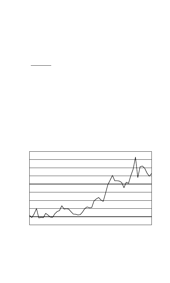
Party Dynamics and Income Inequality
95
survivor benefits, government disability benefits, government pensions,
government educational assistance, Medicare, Medicaid, and food
stamps), minus federal taxes paid. Finally, redistribution is the per-
cent reduction in inequality between pre-redistribution inequality and
post-government inequality:
Pre
− Post
Pre
100
= % Redistribution
(4.1)
More complete details on the creation of these measures are available
in Appendix B.
The paths of pre-redistribution inequality, redistribution, and post-
government inequality over time are charted in Figures 4.1, 4.2,
and 4.3. The pre-redistribution inequality series charted in Figure 4.1
shows relatively steady levels of inequality from the late 1940s to the
early 1970s, at which point a strong trend toward greater inequality is
observed.
7
The year 1951 marked the low point of pre-redistribution
inequality. In this year, the top income quintile had just 2.92 times
as much aggregate income as the bottom two quintiles combined.
2.5
3
3.5
4
4.5
5
5.5
6
6.5
7
1947 1951 1955 1959 1963 1967 1971 1975 1979 1983 1987 1991 1995 1999
T20/B40 Ratio
figure 4.1. Pre-Redistribution Inequality: 1947–2000
7
Inequality of money income actually declined between 1947 and the early 1970s, while
we see that pre-redistribution inequality was stagnant. In both measures the late 1960s
or early 1970s marked a turning point in the path of inequality.
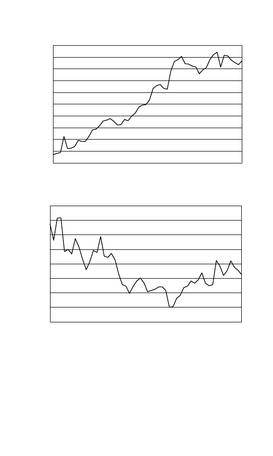
96
The Politics of Income Inequality in the United States
22.5
27.5
32.5
37.5
42.5
47.5
52.5
57.5
62.5
67.5
72.5
1947 1951 1955 1959 1963 1967 1971 1975 1979 1983 1987 1991 1995 1999
Reductio
n
i
n
inequal
it
y
%
figure 4.2. Redistribution: 1947–2000
1.6
1.7
1.8
1.9
2
2.1
2.2
2.3
2.4
1947 1951 1955 1959 1963 1967 1971 1975 1979 1983 1987 1991 1995 1999
T
20/B
4
0
R
ati
o
figure 4.3. Post-Government Inequality: 1947–2000
By 1993, the T20/B40 ratio increased by more than twofold – the
top quintile in that year had nearly seven times as much income as the
bottom two quintiles combined.
That increase in inequality, however, was accompanied by an
increase in the redistributive impact of government. Figure 4.2 shows
almost a straight line toward greater redistribution since 1947. In 1947,

Party Dynamics and Income Inequality
97
government taxes and benefits reduced the ratio of the aggregate
income of the top income quintile to the bottom two income quintiles
by around 25 percent. In 1993 the percentage reduction in inequality
due to explicit redistribution approached 70 percent.
8
Redistribution,
however, did not move in lock-step with pre-redistribution inequal-
ity. The upward trend in redistribution is present even prior to the
increases in inequality in the 1970s. This suggests that redistribution is
not merely an automatic response to increased market inequality but
can also occur in the context of steady levels of inequality.
The recent history of redistribution in the United States is instruc-
tive and appears to be connected with macro political change. After
increasing steadily for four decades, redistribution leveled off during
the Reagan administration. The steady increase in redistribution was
even reversed for a time during Reagan’s second term and George H.W.
Bush’s time in the White House. Redistribution then reached its high-
est point under Bill Clinton and was essentially maintained while he
remained president.
Figure 4.3 charts the level of inequality in the United States after
accounting for the combined impact of market and redistributive mech-
anisms. This chart shows that while pre-redistribution inequality was
remaining steady between 1947 and the early 1970s, increased redistri-
bution pushed post-government levels of inequality markedly lower. In
fact, the decline in post-government inequality continued for several
years after pre-redistribution inequality began increasing. Even into
the late 1970s, post-government inequality was moving lower. Post-
government inequality only began to increase during the Reagan era
in which explicit redistribution came under attack. During the Reagan
and H.W. Bush era, post-government inequality increased and then
essentially stagnated at a new higher level during Clinton’s presidency.
These pictures provide an interesting story in themselves. The visual
evidence seems to argue in favor of the hypotheses of power resources
theory regarding the link between politics and income inequality, but
8
Note that the reduction in the T20/B40 ratio is much higher than the reduction in the
Gini coefficient discussed in Chapter 2. This is the case because the Gini emphasizes
inequality at the middle of the income distribution while the T20/B40 ratio focuses on
the top and bottom of the distribution. Since most redistribution is taking from the
top quintile and giving to the bottom two quintiles, it makes sense that this measure of
redistribution would indicate a higher level of redistribution than when using the Gini.

98
The Politics of Income Inequality in the United States
we can be certain that the paths of distribution and redistribution in
the United States are influenced by more than just politics. For exam-
ple, union membership has been steadily declining at the same time
that inequality has risen and redistribution has increased. Of course
there are other potential explanations that must be considered as well.
This means that rigorous multivariate analysis that takes account of a
variety of explanatory factors is needed.
In this chapter and the next, I will analyze two of the three mea-
sures discussed above as dependent variables – redistribution and
pre-redistribution inequality. These two variables provide the most
direct tests of the theoretical predictions of power resources theory.
Examining the connection between power resources variables and pre-
redistribution inequality provides leverage on the question of whether
lower class power resources influence distributional outcomes via mar-
ket conditioning. If labor union strength and left-party control of
government influence pre-redistribution inequality, this would sup-
port the conclusion that both market and political power resources
influence inequality via a market-conditioning mechanism. The anal-
ysis of political power resources and explicit redistribution provides
a straightforward test of the distributional impact of power resources
via the redistributive mechanism.
Importantly, analyzing these two dependent variables provides
direct evidence about the determinants of post-government inequal-
ity as well. This is the case because post-government inequality is
a direct function of pre-redistribution inequality and redistribution.
Redistribution is calculated based on pre-redistribution inequality and
post-government inequality [Eq. (4.1)]. From this, post-government
inequality can be computed as follows:
Post
= Pre
1
−
Redistribution
100
(4.2)
An increase in pre-redistribution inequality, by definition, produces
an increase in post-government inequality. Contrarily, increases in
redistribution decrease post-government inequality. Thus, the effect
of an explanatory variable on pre-redistribution inequality or redistri-
bution can be directly translated into an impact on post-government
inequality.

Party Dynamics and Income Inequality
99
Control of the Presidency and Distributional Outcomes
To begin the analysis, I examine the bivariate relationship between
party control of the presidency and distributional outcomes. First, I
focus on party control and pre-redistribution inequality. Setting aside
the effects of market power resources and other potentially confound-
ing factors, I ask whether Democratic presidents are associated with
declines in pre-redistribution inequality. Table 4.1 reports the results.
Examining the change in pre-redistribution inequality occurring during
each 4-year presidential term between 1948 and 2000 shows that the
largest 4-year increase in inequality came during Nixon’s ill-fated sec-
ond term. The Democratic presidency of Bill Clinton saw the largest
declines in pre-redistribution inequality. On average, the aggregate
income ratio of the top quintile to the bottom two quintiles declined
by 0.16 during Democratic presidencies and rose by 0.30 under Repub-
lican presidents. This result is consistent with power resources theory,
but is preliminary given the multitude of other factors that might
influence pre-redistribution inequality.
table 4.1. Change in Pre-Redistribution Inequality
by Presidential Administration,
1948–2000
Pre-Redistribution T
20/B40 Ratio
President
First Year
Final Year
Change
Truman (D)
2.95
2.95
0
Eisenhower (R)
2.94
2.97
0.03
Eisenhower (R)
2.96
3.37
0.41
Kennedy/Johnson (D)
3.67
3.46
−0.21
Johnson (D)
3.3
3.16
−0.14
Nixon (R)
3.12
3.6
0.48
Nixon/Ford (R)
3.55
4.09
0.54
Carter (D)
4.17
4.43
0.26
Reagan (R)
4.96
5.2
0.24
Reagan (R)
5.2
4.77
−0.43
H.W. Bush (R)
5.11
5.91
0.8
Clinton (D)
6.65
6.11
−0.54
Clinton (D)
5.97
5.64
−0.33
Republican Average
0.30
Democratic Average
−0.16

100
The Politics of Income Inequality in the United States
table 4.2. Change in Redistribution by Presidential Administration,
1948–2000
Percent Reduction in Inequality via Redistribution
President
First Year
Final Year
Change
Truman (D)
26.6
28.8
2.2
Eisenhower (R)
29.5
31.7
2.2
Eisenhower (R)
33.8
38.4
4.6
Kennedy/Johnson (D)
40.4
40.2
−0.1
Johnson (D)
38.7
40.5
1.9
Nixon (R)
42.4
47.1
4.7
Nixon/Ford (R)
47.3
55.4
8.0
Carter (D)
55.9
61.6
5.8
Reagan (R)
65.6
64.7
−0.9
Reagan (R)
64.5
60.4
−4.1
H.W. Bush (R)
62.1
68.6
6.5
Clinton (D)
69.6
68.0
−1.6
Clinton (D)
66.2
65.9
−0.3
Republican Average
3.0
Democratic Average
1.31
Table 4.2 reports similar data, but examines government redistri-
bution rather than pre-redistribution inequality. Contrary to expec-
tations, we see that redistribution generally increases more under
Republican than Democratic presidential administrations. The evi-
dence on this point, however, is more ambiguous than the evidence on
pre-redistribution inequality. While redistribution increased an aver-
age of 3 points under Republican presidents and only 1.3 points under
Democrats, both the greatest increases and decreases in redistribu-
tion occurred during Republican administrations. The Nixon/Ford
administration oversaw an 8-point increase in the percent reduction
in inequality via government redistribution, which was the largest
increase in any administration. The largest decrease in redistribution
occurred during Reagan’s second term, when redistribution declined
by 4.1 points.
The bivariate results for the connection between party control of
the presidency and pre-redistribution inequality are consistent with
expectations, while the results for redistribution are somewhat puz-
zling. Both results certainly deserve more detailed multivariate analysis,

Party Dynamics and Income Inequality
101
but the redistribution results merit some further discussion at this
point. It is interesting to note that the largest increases in redistribu-
tion occurred during the same period that pre-redistribution inequality
increased most rapidly. This is consistent with the welfare economics
theory of Meltzer and Richard (1981) which predicts that higher lev-
els of inequality will produce greater demand for redistribution. This
is also consistent with the operation of certain social welfare pro-
grams designed as a social insurance safety net. If economic factors
that produce high levels of pre-redistribution inequality also produce
conditions that place more individuals on the public dole, we would
expect to see an increase in redistribution accompany an increase in
pre-redistribution inequality regardless of which party controls the
government because under existing policies more redistribution will
occur naturally.
If such a relationship exists, it presents a catch-22 of sorts for
parties seeking to influence distributional outcomes. Recalling the
two mechanisms through which party control might influence over-
all distributional outcomes – the market and the state – it could be
counterproductive to utilize both mechanisms in tandem. If the pow-
ers of government are used to condition market outcomes in a way
that produces greater pre-redistribution equality, these gains may be
canceled out by corresponding reductions in redistribution. Similar
challenges would face those with inegalitarian goals. In order to sub-
stantively influence overall distributional outcomes (post-government
inequality), policies that avoid this catch-22 are necessary. The trick
is to create redistributive policies that are not driven completely by
pre-redistribution inequality. To learn whether market and political
power resources achieve real influence on distributional outcomes,
more fully specified models must be developed. That is the task to
which I now turn.
A Multivariate Analysis of Lower Class Power Resources and
Distributional Outcomes
I conduct a multivariate analysis of two dependent variables: redistri-
bution, the percent by which government programs decrease inequal-
ity, and pre-redistribution inequality, the distribution of income prior
to the effect of taxes and transfers. Indicators of market and political
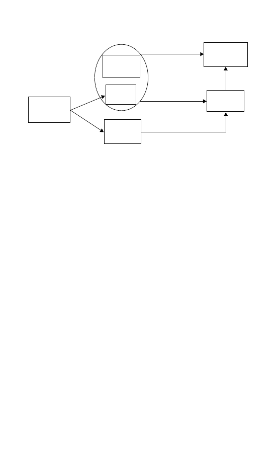
102
The Politics of Income Inequality in the United States
Lower Class
Power
Resources
Union
Strength
Party
Control
Election
Outcomes
Explicit
Redistribution
“Market”
Inequality
figure 4.4. Power Resources Portion of the Model
power resources will be of most central theoretical interest in both
analyses. In this chapter I utilize three standard indicators of political
power resources – Democratic control of the presidency, Democratic
share of seats in the House of Representatives, and Democratic share
of seats in the Senate. I use union membership as an indicator of market
power resources. This analysis is rooted in the overarching theoretical
model first discussed in Chapter 1 and depicted in Figure 1.8. The focus
here is on the aspects of the model that build directly on a classic con-
ception of power resources theory. The specific portion of the model
examined in this chapter is shown in Figure 4.4.
In addition to these classic power resources variables, I also give
attention to variables associated with rival theories, most particu-
larly the logic of industrialism thesis, but also the state-centric theory.
Concepts associated with the logic of industrialism thesis include dein-
dustrialization, economic conditions, and the size and composition of
the labor force. More specifically, I use the following measures to cap-
ture these concepts: the percent of the labor force in nonmanufacturing
jobs, the unemployment rate, the percent of the population over age 65,
the female labor force participation rate, and the percent of the popula-
tion with at least a high school education. In some parts of the analysis,
I include two further measures that have been discussed in the exist-
ing literature on income inequality in the United States (Danziger and
Gottschalk 1995) and could be tied loosely to the logic of industrialism
thesis, but have not generally been discussed in this theoretical context
– the percent of households headed by single females and the percent of

Party Dynamics and Income Inequality
103
the population composed of new immigrants. The state-centric theory
emphasizes state structure as an explanation for state activity. Mea-
sures of constitutional structure are often associated with this theory,
but clearly in a period in which no major constitutional structures were
changed in the United States, this theory is likely less central. However,
I incorporate divided government in my analysis to account for the fact
that the United States has a system of separation of powers.
9
A Brief Methodological Digression: Error Correction Models for
Time Series Analysis
I utilize error correction models (ECMs) to estimate the connec-
tion between indicators of lower class power resources and both
pre-redistribution inequality and redistribution (Banerjee et al. 1993,
Davidson et al. 1978). Given the relatively recent introduction of
these models to political science, a few explanatory details about these
time series models are necessary. ECMs are appropriate when theory
suggests a dependent variable responds to short-term changes in inde-
pendent variables and/or maintains a long-term level consistent with
these variables. This is consistent with the situation in this analysis
because when a shift in partisan control or union strength occurs, there
can be an immediate impact, but additional effects could also be dis-
tributed over time such that the full effect is not fully felt immediately.
I hypothesize that pre-redistribution inequality and redistribution are
responsive to changes in lower class power resources. However, even
if shifts in power resources do not quickly produce different distribu-
tional outcomes, inequality should gradually decrease if high levels of
lower class power resources are maintained.
More specifically, I estimate the short- and long-term effects of
power resources using the single equation method for estimating
ECMs. This strategy is selected in favor of the most common alter-
native, the Engle and Granger (1987) two-step estimator, for two
reasons. First, unlike the two-step method the single equation model
9
None of the models are reported because they produced no significant results and did
not fundamentally alter the substantive results reported. Reporting these results would
have complicated the tables dramatically since interactions between party control and
divided government were included in these models. The additional results did not
justify the added complexity of the tables.

104
The Politics of Income Inequality in the United States
does not impose the assumption of cointegration on the series ana-
lyzed (De Boef and Keele 2008). In fact, the single equation ECM is a
modified version of an autoregressive distributed lag model in which
the dependent variable is a function of its past values and past val-
ues of the independent variables. This means that the single equation
ECM can be applied to both integrated and stationary series (Banerjee
et al. 1993, De Boef 2001, De Boef and Granato 1999, De Boef and
Keele 2008). Second, the single equation estimator is preferred in small
samples (Banerjee 1986, De Boef and Granato 1999). Overall, use
of the single equation model can be justified in a broader range of
circumstances than the two-step method.
10
One way to express a bivariate single-equation error correction
model is as follows:
Y
t
= β
1
X
t
−i
− β
2
(Y
t
−1
− β
3
X
t
−1
− λ) +
t
(4.3)
In words, this equation simply tells us that changes in a dependent
variable Y are determined by short-term changes in an independent
variable X as well as divergence from a long run equilibrium between
X and Y. Imagine, for example, that a change in short-term interest
rates is connected to long-term interest rates by an error correction
mechanism. Long run rates might rise in response to a change in short-
run rates (with the value of i determining the lag before the onset of this
“short-term” effect). But that may not be the only connection between
the variables. It is also possible (in fact more likely based on empirical
analysis) that short and long rates maintain an equilibrium relation-
ship such that disturbing short-term rates creates a situation in which
long-term rates are too low relative to short-term rates. Over time,
10
ECMs are also a way to correct for any problems of nonstationarity in a dependent
variable. If a dependent variable has a deterministic trend such as increasing con-
sistently over time or contains a data generating process that produces some other
form of nonstationarity, statistically significant results can be spurious and lead to
incorrect inferences. This is obviously a situation to be avoided. The classic solution
for a nonstationary dependent variable is to analyze the first difference, or change,
in the dependent variable. In an ECM, change in the dependent variable is analyzed,
so nonstationarity is generally not a problem. However, it is theoretically possible
though extremely rare for a differenced dependent variable to be nonstationary. To
guard against this situation I tested all of my differenced dependent variables for sta-
tionarity. Multiple tests (including Dickey-Fuller, Phillips-Perron, and Kwiatkowski,
Phillips, Schmidt, and Shin) confirm that analyzing change in redistribution and
change in pre-redistribution inequality satisfies the stationarity requirement.

Party Dynamics and Income Inequality
105
this deviation (error) from the long run equilibrium will be eliminated
(corrected) by an increase in long-term rates. An ECM takes account of
both possible mechanisms. The first type of connection is captured by
the effect of changes in short-term rates on changes in long-term rates.
The second type of connection is captured by examining the lagged
distance between short- and long-term rates in levels.
In the analysis below, I utilize the following transformed version of
equation (4.3) to estimate ECMs:
Y
t
= α
0
+ α
1
Y
t
−1
+ β
1
X
t
−i
+ β
2
X
t
−1
+
t
(4.4)
For each independent variable X, then, we have up to two parameter
estimates –
β
1
for the differenced variable, its change from one point
in time to the next, and
β
2
for the lagged level of the variable.
11
But
what do these two parameter estimates mean? In this simple bivariate
example,
β
1
provides an estimate of the initial change in the dependent
variable produced in the short term by a shock to the independent vari-
able.
12
For example, if public opinion shifts in a liberal direction and
policymaking responds by shifting in the same direction, the short-
term coefficient,
β
1
, provides an estimate of the size of this shift. To
explain some terminology that will be used extensively in the remain-
der of the book, then, this is the type of effect that will be referred to as
the “short-term” effect. This does not mean that the effect is imperma-
nent, but simply that the effect happens all at once at a specified point
in time.
β
2
provides a portion of the information needed to estimate the
“long-term” impact, which is slightly more complicated to explain.
This is also called the error correction component of the model. The
long-term impact is the portion of the connection between X and Y that
does not occur at a particular point in time but is distributed temporally
such that a portion of the impact is felt in each period over a time span.
Returning to a substantive example, if the impact of public opinion is
11
The lagged level can be dropped from the equation if we find that it has no statistically
significant impact.
12
The onset of this initial impact could be contemporaneous, with a shift in the inde-
pendent variable at time t creating a shift in the dependent variable at time t. It could
also be lagged, such that the initial shift in the dependent variable may not occur for
some specified number of time periods; thus the t
− i subscript on the X parameter.

106
The Politics of Income Inequality in the United States
linked to policymaking via an error correction mechanism, a shock
to public opinion disturbs the long run equilibrium between opinion
and policy, and this divergence from the equilibrium will eventually be
corrected over time. The size of this long run impact is a function not
only of
β
2
but also of
α
1
, which is known as the error correction rate.
The full long-term impact of a shock to X on Y via the error correction
component, known as the long run multiplier, is computed by dividing
β
2
by
α
1
.
Aside from being a component in the computation of the impact
(via the error correction mechanism) of the independent variable on
the dependent variable, the error correction rate (
α
1
) also tells us some-
thing about how quickly a disturbance from the long run equilibrium is
eliminated. Estimates of
α
1
will in practice be between 0.0 and
−1.0 in
appropriately specified ECMs, and the closer this parameter is to
−1.0,
the more quickly errors are corrected. The substantive interpretation
of the coefficient is the proportion of the disturbance from equilibrium
that will be corrected in each time period, beginning at t
+1. From this
error correction rate, we can then make inferences about how quickly
the total long run impact is felt.
I will often utilize terminology from the ECM tradition to describe
the results. “Short-term” effects refer to the initial impact of X on
Y. “Long-term effects,” “effects via the error correction mechanism,”
and “the long run multiplier” all refer to the effect of X on Y that is
distributed over time. Finally, “total effects” refer to a combination of
short- and long-term effects. I turn now to the heart of the analysis.
Analyzing Redistribution
I begin by examining the determinants of the redistributive impact
of government, which is the classic dependent variable in the power
resources theory tradition. Redistribution, as defined above, is mea-
sured as the percentage reduction in the ratio of the income of the
top income quintile to the income of the bottom two quintiles that
is attributable to government taxes and benefits. Table 4.3 reports
the results of two ECM models of government redistribution. In
each of these models, the variables most central to testing power
resources theory are the indicators of political power resources. The
expectation is that Democratic Party control of government should

table 4.3. Explaining Government Redistribution,
1947–2000
Redistribution
Independent Variables
(1)
(2)
Error Correction Rate
−0.30
∗∗
−0.37
∗∗∗
(0.13)
(0.12)
Political Power Resources
Democratic President
t
−1
0.54
0.02
(0.74)
(0.72)
Democratic President
t
−1
1.10
∗
1.17
∗∗
(0.57)
(0.48)
% Senate Democrat
t
−1
0.01
(0.07)
% Senate Democrat
t
−1
−0.09
(0.06)
% House Democrat
t
−1
0.08
(0.06)
% House Democrat
t
−1
0.04
(0.07)
Labor Market Factors
% Unemployed
t
1.64
∗∗∗
0.66
∗∗∗
(0.55)
(0.23)
% Unemployed
t
−1
0.62
∗
0.56
∗
(0.35)
(0.31)
% Nonmanufacturing
t
−1.06
(0.66)
% Nonmanufacturing
t
−1
−0.10
(0.29)
Demographic Factors
% Aged 65+
t
−0.36
7.52
∗
(5.75)
(3.85)
% Aged 65
+
t
−1
3.71
∗∗∗
2.99
∗∗∗
(1.20)
(0.96)
% New Immigrants
t
−0.58
(1.24)
% New Immigrants
t
−1
−1.85
(1.21)
Response to Inequality
Pre-Redist. Inequality
t
4.57
∗∗∗
5.04
∗∗∗
(0.87)
(0.77)
Pre-Redist. Inequality
t
−1
−1.14
(0.99)
Constant
−12.69
−17.02
∗∗∗
(17.27)
(5.98)
Adj. R
2
0.79
0.77
N
52
52
Two-tailed significance levels:
∗
p
≤ 0.10;
∗∗
p
≤ 0.05;
∗∗∗
p
≤ 0.01.
Note: Table entries are time series regression coefficients representing a single-equation
error correction model with standard errors in parentheses.

108
The Politics of Income Inequality in the United States
increase the equalizing influence of government. I begin with an over-
specified model of redistribution to provide a rigorous test of power
resources theory versus alternative explanations and then proceed to
a reduced form model that presents the most parsimonious model of
redistribution.
Model 1 represents the most fully specified model. In addition to
Democratic control of the presidency and shares of Democratic seats
in the Senate and in the House, I include a variety of variables that are
related to the logic of industrialism hypothesis. I organize these vari-
ables into two further categories: labor market factors (unemployment
and deindustrialization) and demographic factors (population aged 65
and over and immigration). Unemployment should increase redistri-
bution because increases in unemployment will automatically generate
unemployment insurance payments. Deindustrialization might have
a similar impact, as manufacturing workers are displaced and need
retraining to obtain new employment. The size of the elderly pop-
ulation should also increase redistribution given the importance and
magnitude of programs targeted toward this constituency such as
Medicare and Social Security. McCarty et al. (2006) argue that immi-
gration should influence redistributive policy. In addition to these
variables that are related to the logic of industrialism thesis, I include a
control for pre-redistribution inequality with the idea that higher levels
of inequality will generate greater redistribution because of formulaic
policies activated by the same conditions that generate high levels of
pre-redistribution inequality.
The results for Model 1 support the predictions of power resources
theory as well as some of the predictions of the logic of industrial-
ism. First and foremost, the coefficients reported at the top of the
table show that Democratic control of the presidency increases redis-
tribution in the long term. Also as expected, the unemployment rate,
the elderly population, and pre-redistribution inequality increase gov-
ernment redistribution. However, we observe no significant impact
of partisan strength in Congress on redistribution in either the short
or long term, and the same can be said for deindustrialization and
immigration.
13
Model 1, then, is over-specified.
13
These results would be even more supportive of power resources theory if partisan-
ship of both the presidency and Congress influenced explicit redistribution. As it

Party Dynamics and Income Inequality
109
A more restricted model is reported in the next column. Deindus-
trialization and partisan strength in Congress, along with the estimate
of the nonsignificant long-term impact of pre-redistribution inequality,
are dropped from the earlier model to produce a more parsimonious
and efficiently specified model of redistribution. This model includes
just four explanatory variables – Democratic control of the presidency,
the unemployment rate, the elderly population, and pre-redistribution
inequality. The model estimated is as follows, dropping insignificant
coefficients for the sake of simplicity:
Redist
t
= −17.02 + .66Unemp
t
+ 7.52Elderly
t
+ 5.04Pre
t
− .37Redist
t
−1
+ 1.17DemPres
t
−1
+ .56Unemp
t
−1
+ 2.98Elderly
t
−1
+
t
(4.5)
As in the first model, Democratic control of the presidency pro-
duces a long-term increase in redistribution. This supports the central
prediction of power resources theory. The two coefficients estimated
for Democratic president and the estimate of the error correction rate,
stands, only the presidency matters, and this result is repeated in the later analysis
of pre-redistribution inequality. While the fact that the proportion of seats held by
Democrats in the House and the Senate does not directly influence distributional
outcomes is not supportive of power resources theory, neither do the insignificant
results disprove power resources theory. It is still somewhat puzzling why no effect
can be found for left party strength in Congress. In fact, I have tried a variety of
specifications and measurement strategies to account for Democratic presence in the
legislative branch. I included dichotomous variables for party control of the House,
the Senate, and Congress as a whole. I have even diverged from a direct measure
of partisanship to examine ideological common space scores. I have also utilized
strategies that account for the super-majoritarian nature of the Senate and the role of
divided government. Regardless of the strategy, no significant results can be found for
the legislative branch. It may be the case that I have overlooked a method of modeling
the partisan composition of Congress. It might also be that the president has such
a degree of agenda control that it is actually correct to conclude that only the par-
tisanship of the president matters directly for determining distributional outcomes.
However, we will see in the next chapter that macro policy influences distributional
outcomes. Since the partisan composition of Congress has been previously shown to
influence macro policy (Erikson et al. 2002), it would be inappropriate to conclude
that Congress has no role in shaping distributional outcomes. I do not explore the
underlying reasons for this null result because such an exploration is more relevant to
theories of policy making than to power resources theory, which is my primary focus
here. This remains an interesting question that might be worthy of future exploration
in a different theoretical context.

110
The Politics of Income Inequality in the United States
which is 37 percent annually, give us a great deal of substantive infor-
mation. When a Democratic president is elected, this shift in party
control does not have an immediate impact. However, over the course
of time, the shift to a Democratic president increases redistribution by
3.16 points. More tangibly, if government is already reducing inequal-
ity through redistribution by 23 percent, when a Democrat takes over
the presidency from a Republican, government reduction of inequal-
ity will increase to more than 26 percent over the course of about 8
years. This is a substantial impact given that redistribution changes on
average each year by less than 2 points.
While the total effect of Democratic control of the presidency is
a 3.16 point increase in redistribution, it is important to remember
that this impact is distributed over time, such that only 37 percent
of the disequilibrium is corrected each year, beginning the year after
control of the presidency changes. Thus, the first year after a Demo-
cratic takeover (year two of an administration), the model predicts a
1.17 point increase in redistribution. After this impact, a 1.99 point
disequilibrium remains, 37 percent of which, or 0.74 points, is cor-
rected in the second year after a Democratic takeover of the White
House. Continuing this pattern, redistribution increases 0.46 points in
the third year after Democratic control occurs. Thus, over the course of
a first presidential administration, the effect of Democratic as opposed
to Republican control totals a 2.37 point increase in redistribution.
The total effect of two consecutive Democratic administrations is a
3.09 point increase. This effectively tells us that 75 percent of the total
impact of a shift in presidential control occurs during the first term of
a president, while nearly 98 percent of the total impact is felt over the
course of two administrations. These results also indicate that main-
taining a shift in party control for a third presidential term would have
little additional impact on government redistribution, at least through
the direct mechanism analyzed here. Democratic control for a third
presidential term would, of course, maintain the same level of redistri-
bution, while switching to Republican control would result in a decline
in the level of redistribution.
The results reported in the table focus on variables related to
power resources theory and the logic of industrialism thesis. I also
entertained models including variables related to state-centric theories
of welfare state activity. State-centric theories focus on institutional

Party Dynamics and Income Inequality
111
characteristics of government organization in explaining welfare state
development. Given my focus on one country over time, during a
period in which institutional structures remained essentially constant
at the national level, meaningful state-centric variables are few. I did,
however, consider divided government as a way to tap the effect of the
separation of powers institutional arrangement of the United States.
In addition to the variables included in Model 2 of Table 4.3, I added
an indicator of divided government, as well as an interaction term of
divided government and Democratic control of the presidency. The
goal here was to determine whether the substantive impact of party
control of the presidency is augmented during times of unified gov-
ernment. Adding dividing government and the interaction term added
no explanatory power to the model, and none of the additional vari-
ables were significant. Thus, these results fail to lead to any additional
insights, other than to say that there is no support for the conclu-
sion that the impact of political power resources are conditioned by
divided or unified government. This may not be surprising given the
limited impact of party strength in Congress in the earlier models.
Analyzing Pre-Redistribution Inequality
In the analysis above, I addressed the question of whether political
power resources influenced the path of government redistribution in
the post–World War II United States. The answer is a resounding yes.
These results show that the most fundamental prediction of power
resources theory applies in the context of the United States, and the
findings are broadly consistent with similar analyses conducted using
shorter time periods and different indicators of welfare state effort
(Hibbs and Dennis 1988, Kelly 2004). Now, I turn to an analysis of a
more novel implication of power resources theory – that both market
and political power resources influence pre-redistribution inequality.
This analysis addresses the question of whether state activity influences
income inequality through market conditioning in addition to the more
traditional mechanism of explicit redistribution.
Table 4.4 reports the results of five error correction models of pre-
redistribution inequality.
14
In this analysis, I present four preliminary
14
It is possible that distributional outcomes such as pre-redistribution inequality influ-
ence lower class mobilization that translate into the indicators of power resources

table
4
.4
.
Explaining
Pre-Redistribution
Inequality,
1947
–2000
Pre-Redistribution
Inequality
Independent
Variables
(1)
(2)
(3)
(4)
(5)
Error
Correction
Rate
−
0.39
∗∗∗
−
0.81
∗∗∗
−
0.52
∗∗∗
−
0.76
∗∗∗
−
0.74
∗∗∗
(0.14
)(
0.16
)(
0.14
)(
0.13
)(
0.13
)
Political
Power
Resources
Democratic
President
t−
1
−
0.27
∗
−
0.34
∗∗∗
−
0.23
∗
−
0.28
∗∗∗
−
0.30
∗∗∗
(0.14
)(
0.12
)(
0.12
)(
0.09
)(
0.09
)
Democratic
President
t−
1
−
0.07
0.07
0.01
(0.10
)(
0.09
)(
0.09
)
%
Senate
Democrat
t−
1
−
0.02
(0.02
)
%
Senate
Democrat
t−
1
−
0.00
(0.01
)
%
House
Democrat
t−
1
0.01
(0.01
)
%
House
Democrat
t−
1
0.00
(0.01
)
Market
Power
Resources
%
Unionized
t−
1
0.03
0.01
0.01
0.02
0.02
(0.08
)(
0.07
)(
0.07
)(
0.06
)(
0.06
)
%
Unionized
t−
1
−
0.06
∗∗∗
−
0.08
∗∗
−
0.05
∗
−
0.10
∗∗∗
−
0.09
∗∗∗
(0.02
)(
0.04
)(
0.03
)(
0.02
)(
0.02
)
Labor
Market
Factors
%
Unemployed
t−
1
0.19
∗∗
0.10
0.05
(0.09
)(
0.08
)(
0.03
)
%
Unemployed
t−
1
0.10
∗
0.11
∗∗∗
0.10
∗∗∗
(0.05
)(
0.03
)(
0.03
)

.
%Nonmanufacturing
t−
1
−
0.20
∗
−
0.07
(0.11
)(
0.10
)
%
Nonmanufacturing
t−
1
0.07
(0.06
)
Female
Labor
Part
t−
1
−
0.04
(0.11
)
Female
Labor
Part
t−
1
0.00
(0.02
)
Demographic
Factors
%
Aged
65
+
t−
1
0.97
(0.87
)
%
Aged
65
+
t−
1
−
0.27
(0.27
)
%
New
Immigrants
t−
1
−
0.84
∗∗∗
−
0.70
∗∗∗
−
0.73
∗∗∗
(0.25
)(
0.21
)(
0.20
)
%
New
Immigrants
t−
1
0.64
∗∗∗
0.41
∗∗
0.46
∗∗∗
(0.22
)(
0.19
)(
0.17
)
%
SF
Headed
HH
t−
1
−
0.10
(0.14
)
%
SF
Headed
HH
t−
1
0.11
(0.08
)
Constant
3.25
∗∗∗
−
0.34
3.39
∗
4.94
∗∗∗
4.67
∗∗∗
(1.09
)(
4.83
)(
1.90
)(
1.01
)(
0.93
)
Adj.
R
2
0.22
0.45
0.33
0.56
0.57
N
52
52
52
52
52
Two-tailed
significance
levels:
∗
p
≤
0.10
;
∗∗
p
≤
0.05
;
∗∗∗
p
≤
0.01
.
Note:
Table
reports
time
series
regression
coefficients
representing
a
single-equation
error
correction
model
with
standard
errors
in
parentheses.

114
The Politics of Income Inequality in the United States
models that include subsets of explanatory factors to assess the sensi-
tivity of the effect of the primary theoretical variables to specification.
The indicators of market and political power resources are included in
every model.
Model 1 examines the impact of market and political power resources
on pre-redistribution inequality in isolation from other potential
explanatory factors. In a nutshell, both market power resources, in the
form of union membership, and political power resources, in the form
of Democratic control of the presidency, influence pre-redistribution
inequality. Democratic strength in the Congress, however, has no dis-
cernible impact, so these variables are dropped from the remaining
models. It is worthy to note that a wide variety of measurement strate-
gies for Congressional party strength were employed, from simple party
control of the House and the Senate to measures that accounted for
the super-majoritarian nature of policymaking in the Senate, and all
produced identical results.
15
Model 2 considers three measures of labor market characteristics –
unemployment, deindustrialization, and female labor force participa-
tion – in addition to the statistically significant indicators of market
and political power resources included in Model 1. Unemployment
and deindustrialization were also considered as explanations of redis-
tribution in the earlier analysis, but female labor force participation
is a variable that has received greater attention in studies attempting
to explain income inequality as opposed to government redistribution.
Thus, I also consider it here alongside the other labor market factors. In
this model both market and political power resources remain important
determinants of pre-redistribution inequality. In addition to the power
resources variables, unemployment and deindustrialization also have
a statistically significant impact on pre-redistribution inequality. Thus,
these variables will be included in the final model, but for deindustri-
alization only the immediate impact will be considered since Model
2 shows that this variable has no additional long-term impact that is
theory. This could create simultaneity bias in the models that I estimate. To guard
against this I lag the impact of change in power resources variables on change in
distributional outcomes. It is not likely that changes in power resources this year are
influenced by changes in distributional outcomes next year.
15
See footnote 13 for a discussion of this null result.

Party Dynamics and Income Inequality
115
phased in over time (as evidenced by the insignificant coefficient for
lagged levels of nonmanufacturing jobs).
Model 3 removes labor market factors and considers three demo-
graphic factors that have been suggested as determinants of income
inequality – the elderly population, immigration, and single-female
headed households. Each of these factors is expected to increase
inequality. Of these variables, immigration is the only factor that
influences pre-redistribution inequality. Interestingly, the short- and
long-term impact of immigration work against each other. While the
initial impact of an increase in immigration is a decline in inequality,
this decline is eventually canceled out and, in fact, reversed over time.
The short-term, negative impact is
−0.84, while the total long-term
impact is 0.64
/0.52 = 1.21. The immediate and long-term impact of
immigration are carried into Model 4.
Model 4 simply puts the previous three models together to provide
an assessment of pre-redistribution inequality that considers politi-
cal power resources, market power resources, labor market factors,
and demographic factors in a single model. When considered jointly,
the main results of theoretical interest remain, but deindustrialization
loses its explanatory significance in this model. These first four models
show that the impact of lower class power resources is robust. Regard-
less of which economic and demographic controls are included in the
model, the impact of party control of the White House and union
strength on inequality is consistent. Model 5 presents a final analysis of
pre-redistribution inequality, which represents the most parsimonious
model.
This final model produces results that are consistent with power
resources theory. First, we see that union membership has a nega-
tive impact on pre-redistribution inequality. This provides support
for a classic power resources theory prediction. Second, and even
more importantly, this model shows that political power resources
in the form of Democratic control of the presidency also influence
pre-redistribution inequality. This supports the conclusion that state
activity influences distributional outcomes via market conditioning
in addition to the more traditionally conceptualized mechanism of
explicit redistribution. Democratic control of the presidency increases
explicit redistribution, but also decreases pre-redistribution inequality.

116
The Politics of Income Inequality in the United States
Explicit redistribution and market conditioning are two distinct mecha-
nisms for distributional impact that are used in tandem to influence the
path of income inequality in the United States. Interestingly, the impact
of party control on pre-redistribution inequality is immediate, while the
impact on redistribution is distributed over time. When a Republican
takes over the White House, this analysis shows that pre-redistribution
inequality will increase by 0.30 points in the year after party control
changes. This is a large impact given that pre-redistribution inequality
only goes up or down by an average of 0.22 points each year. However,
it takes two full presidential terms for the total impact of party control
on redistribution to be observed. This seems to indicate, at least with
regard to the direct effect of party control on distributional outcomes,
that changes in redistribution are politically difficult to generate, while
conditioning market outcomes can be achieved more directly, easily,
and quickly.
Other than power resources explanations, only the rate of unem-
ployment and immigration have a statistically significant impact on
pre-redistribution inequality in the fully specified model. In this case
the impact of unemployment is substantively powerful in only its
long-term impact. A 1 percent increase in unemployment increases
pre-redistribution inequality by less than half the amount produced
by a shift from Democratic to Republican control of the presidency.
As mentioned earlier, the short- and long-term impact of immigration
work against each other. An increase in immigration leads to an ini-
tial increase in inequality that is essentially erased by later increases
in inequality over the long term. Finally, as with explicit redistribu-
tion, in models not shown, I considered divided government and its
interaction with party control as potential explanatory factors. No
results of interest were produced. Either divided government is not
consequential or the data analyzed here are simply not of high enough
quality to produce confirmation of the importance of the separation of
powers.
conclusion
The most important message of this chapter is that power resources the-
ory can be effectively applied in the context of the United States. Despite
several factors that make the United States a challenging context in

Party Dynamics and Income Inequality
117
which to analyze power resources theory, its central predictions hold
true. Market power resources in the form of union membership drive
down the level of inequality produced within the market. Political
power resources influence the amount of redistribution generated by
the state, with the direct effect of Democratic strength being an increase
in redistribution.
I went beyond these two traditional predictions of power resources
theory, however, and the analysis produced some surprising results.
Specifically, I hypothesized that political power resources would be
used to influence market action as well as government activity. Rooted
in my discussion of market conditioning as a mechanism of distribu-
tional impact in Chapter 2, it seems reasonable to suspect that control
of the state by lower class interests would produce an equalizing impact
via both market conditioning and explicit redistribution. I tested this
hypothesis by examining the connection between indicators of lower
class power resources and inequality measured prior to the effects
of government taxes and benefits. The results lead to the conclusion
that party control of government matters for both redistribution and
government conditioned market inequality, meaning that market con-
ditioning and redistribution are tools of state distributional impact.
Even before redistribution occurs, government matters.
The primary political variables of interest in this chapter were the
relative strength of the two major parties in government. Clearly, parti-
san dynamics matter, and such an emphasis on party control is closely
connected to previous studies in the power resources tradition. The
reason power resources theory suggests that party control should mat-
ter for distributional outcomes, of course, is that different parties will
pursue different policies. Policies, however, are rarely assessed directly
in cross-national studies of power resources theory. Assessing policy is
important because the U.S. parties do not always consistently support
or oppose redistribution and reductions in inequality. Bill Clinton, for
example, was a Democrat who supported welfare reform measures
that made it harder for the poor to remain on the welfare rolls. This
was not a classic redistributional stance by a Democrat. In the next
chapter, I account for such policy variation by focusing explicitly on
the ideological tone of policy as a more proximate cause of distribu-
tional outcomes than partisanship. In doing so, I bring a major theory
from comparative politics into direct communication with the macro
politics model of U.S. politics.

5
Macro Policy and Distributional Processes
The theoretical focus of the previous chapter was on power resources.
There we saw that the fundamental predictions of power resources
theory for distributional outcomes are borne out in the United States.
Market and political power resources, as traditionally measured, have
an impact on income inequality. Labor union strength influences
income inequality measured prior to government redistribution. Left
party control produces lower levels of inequality through both mar-
ket conditioning and explicit redistribution. In this chapter, I shift the
emphasis from power resources theory, an idea originating in the com-
parative study of welfare states, to the macro politics model, which has
its roots in studies of American politics.
As discussed in Chapter 1, the macro politics model examines rela-
tionships between parts of the U.S. governing system, such as public
opinion, presidential approval, partisanship, elections, and public pol-
icy at the aggregate level. The argument is that the parts of the system
behave predictably and orderly. Citizens express preferences about
competing policy alternatives, the preferred alternatives are enacted,
and citizens then judge the quality of the outcomes produced. Tests of
this model show that liberal shifts in public opinion produce liberal
shifts in policy because policymakers respond to changes in pub-
lic opinion and, if they do not, they are replaced through popular
elections.
Aggregate public opinion influences the course of public policy in the
United States, and this previous finding is an important underpinning
118

Macro Policy and Distributional Processes
119
of my work. But the macro politics model in essence assumes that
changes in public policy produce changes in societal outcomes (though
see Kellstedt et al. 1993). Based on the discussion in Chapter 3, it
should be clear that in the realm of income inequality, shifts to the left
in public policy are expected to produce reductions in income inequal-
ity. However, this implication of the macro politics model has not
been rigorously tested (Figure 1.6). If citizens exert influence over pub-
lic policy but policy does not influence important societal outcomes,
the substantive impact of the opinion-policy link declines. My goal in
this chapter is to determine whether the ideological content of policy,
rather than partisan control, systematically influences distributional
outcomes.
micro and macro: the logic of macro politics
At its heart, the macro politics model is about how the governing sys-
tem of the United States functions. Ideally, a democratic system would
be composed of highly informed and active citizens who influence the
behavior of policymakers and hold them accountable for their actions.
Decades of individual-level survey research, however, have shown that
the ideal citizen at the heart of this picture is a rare bird. The empirical
debunking of the democratic ideal in American politics is rooted in
the individual voting behavior tradition. Beginning with the Columbia
studies of the 1940s and continuing with the publication of The Amer-
ican Voter (Campbell et al. 1960), a venerated line of research in
political science has raised a variety of problems regarding the trans-
lation of citizen preferences into public policy. The problem is that
individual citizens in the United States are not particularly informed
about contemporary policy issues, do not appear to care all that much
about who wins election contests, and do not organize their political
ideas around an ideology in ways that facilitate the communication of
policy preferences through voting at the polls. Since elections are the
only formal mechanism for control of public policy by citizens, these
consistently confirmed findings about the individual voter in the United
States are troubling.
A new and different research paradigm in political science began
to take shape in the late 1980s (Erikson et al. 2002, Page and
Shapiro 1992, Stimson 1999, Stimson et al. 1995, Wlezien 1995).

120
The Politics of Income Inequality in the United States
This new research moved the emphasis from the micro-level individual
voter to the macro-level citizenry as a collective. Research in this
macro tradition, though not questioning the view of the individual
voter developed in the previous four decades, does raise problems with
the system-level conclusions that micro studies suggest. The micro tra-
dition essentially concludes that meaningful democratic control of pub-
lic policy is impossible, but the macro tradition questions whether the
aggregation of mostly uninformed, uninterested, and nonideological
voters produces an uninformed, uninterested, and nonideological elec-
torate. According to macro analysis, the problem with drawing infer-
ences about the political system based on the typical voter described in
micro analyses is the surprising finding that atypically informed citizens
drive the overall tendency of aggregate public opinion.
The theoretical argument of the macro paradigm is as follows.
Democracy has both an individual and a collective component. Demo-
cratic theory in part calls on government to be responsive to the
preferences of individual citizens, but the translation of collective
preferences into collective outcomes is more central to democracy.
Research at the individual level clearly shows that most people are
not enlightened in the sense of caring deeply about political issues and
of fitting preferences in one arena together with preferences in another.
In other words, individual preferences are noisy and contain a mini-
mal, if any, policy signal. However, one must be mindful of the fact
that government responsiveness to citizen preferences is an aggregate
phenomenon, and it is important to note that there are some citizens
who go against the norm, having large amounts of political interest
and information and adopting their political preferences around logical
ideologies.
When uninformed citizens change their preferences, they do so in an
essentially random way because there is no underlying organizational
principle for these citizens’ opinions. Highly informed and ideologically
oriented citizens, on the other hand, make predictable and consistent
changes in their issue preferences across a variety of policy domains.
Therefore, any change in aggregate public opinion that is observed
from one time to the next cannot be driven by uninformed citizens
because their opinion changes are random, with one person’s random
change canceling out another’s random change. Instead, aggregate
opinion change is driven by the highly informed who transmit less

Macro Policy and Distributional Processes
121
error-laden opinions and, thus, carries a meaningful policy signal (the
public mood) that can be communicated through elections. This is why
aggregate preferences on a wide array of domestic policy issues in the
United States move together over time in orderly and predictable ways
despite the true finding that most individual citizens do not possess
orderly and predictable preferences.
1
In sum, quantitative analyses of the individual voter in the United
States debunked democratic theory’s view of the enlightened citizen,
but the new conceptualization and measurement of public opinion
developed in the macro paradigm rescued democratic theory’s view
of the enlightened citizenry. The macro conception of public opinion
forcefully demonstrates that it is theoretically possible for the U.S. elec-
torate to send meaningful policy messages to government officials. At
the aggregate level, public opinion sends an ideologically directed signal
about preferred public policies. When attitudes on one political issue
move toward the ideological left, attitudes on other issues generally
follow a similar path (Stimson 1999).
The macro politics model does not stop by demonstrating that aggre-
gate public opinion projects ideological preferences, but builds on this
fundamental finding by assessing the impact of the public mood on pol-
icymaking. The question is whether the ideological content of public
opinion influences the ideological direction of public policy (Erikson
et al. 2002, Stimson et al. 1995). Using policymaking data from all
three constitutional branches of government, research in the macro pol-
itics tradition shows that when public opinion shifts to the left, public
policy responds in the same direction. For the elected branches of gov-
ernment, this popular influence over policymaking occurs through two
paths. First, elections provide an opportunity for the citizenry to place
like-minded representatives in charge of government. Second, because
of the re-election motive of elected officials, public policy responds
to shifts in public opinion between elections. Interestingly, there is evi-
dence that the decisions of the unelected judicial branch, likely because
of its need to maintain legitimacy with the mass public and elected
1
Enns and Kellstedt (2008) tell a theoretically different story that leads to the same
fundamental conclusion. They show that people at all levels of political sophistication
receive information and change their opinions in similar ways. Under this conception
of macro opinion change, aggregate opinion is perhaps even more meaningful.

122
The Politics of Income Inequality in the United States
officials, is responsive to public opinion (Erikson et al. 2002, McGuire
and Stimson 2004, Stimson et al. 1995).
Research in the macro politics tradition demonstrates that, at the
aggregate level, changes in public opinion produce changes in public
policy. This evidence is used to support the conclusion that the U.S.
governing system provides a large measure of democratic control over
the government – that the U.S. governing system fosters democratic
representation. While this is probably a correct conclusion, it is impor-
tant to remember that democratic control of government is normatively
important largely because of the influence and power that government
wields over society. So, democratic theory is really about more than
determining the policies that government enacts. It is also about the
influence that government has on society through these policies. Ideally,
it is this influence on society that citizens are able to control through
public policy.
While it may be true that aggregate public opinion influences the
course of public policy in the United States, the macro politics model
leaves the question of whether or not changes in public policy produce
changes in societal outcomes largely untested. In the realm of income
inequality, a leftward shift in policy should produce quite different
distributional consequences than a move to the right according to the
macro politics model. If citizens exert influence over public policy, but
public policy does not influence important societal outcomes, then the
importance of the representation for which the macro politics model
finds support is minimized. It is wonderful that citizens influence pub-
lic policy, but this fact matters little if public policy does not exert
systematic influence on societal outcomes over which there is political
contestation. I extend the macro politics model by examining whether
income inequality in the United States has been systematically and pre-
dictably influenced by the ideological direction of public policy during
the post-World War II era.
macro politics, power resources, and the
distributional consequences of policy
While the theoretical emphasis in this chapter is the macro politics
model rather than power resources theory, these theories need not be
viewed in isolation from one another – the analysis of this chapter, in

Macro Policy and Distributional Processes
123
fact, builds directly on the previous chapter. The macro politics model
is broad in its scope of analysis, examining as many aspects of the Amer-
ican governing system as possible. Power resources theory, on the other
hand, is focused on class conflict and distributional outcomes. Despite
these differences, I combine the two theories to provide a more com-
plete picture of distributional processes. Left party control is a central
indicator of lower class power resources in power resources theory,
and this was the key explanatory concept in the previous chapter’s
analysis. But election outcomes, as a path that connects public opinion
and policy outputs, are also an important component of the macro pol-
itics model. The macro politics model speaks of “election outcomes”
and power resources theory discusses “party control of government.”
As Figure 1.8 depicted, these are identical concepts that create a
direct overlap between the macro politics model and power resources
theory.
Chapter 4, in part, presented a straightforward test of two central
predictions of power resources theory – that left party control of gov-
ernment will produce greater government redistribution and will also
lower overall levels of income inequality. This fundamental expec-
tation was supported by the analysis. The evidence presented in the
previous chapter can also be interpreted as supportive of the macro
politics model. Party control of the policymaking institutions of gov-
ernment, produced by election outcomes, is one part of the macro
politics model. Showing that Democratic control of the presidency
produces more redistribution and less inequality is certainly consis-
tent with the macro politics model. But in the macro politics model,
election outcomes are merely a precursor to the ultimate outcome of
the political system – public policy (Erikson et al. 2002). Thus, my
focus on the connection between public policy and distributional out-
comes in this chapter provides a fairly straightforward extension of the
macro politics model.
Examining the link between public policy and inequality is not only
a direct extension of previous studies of U.S. macro politics, but can
also be linked to power resources theory. The macro politics model and
power resources theory overlap quite neatly with respect to party con-
trol of government, and they also overlap with respect to the analysis
of public policy.

124
The Politics of Income Inequality in the United States
Most conceptions of power resources theory consider public pol-
icy as an output that varies depending on the constellation of power
resources. Under this view the state is an instrument for the exercise
of power resources, and indicators of power resources such as left
party strength in government are used to explain state action. Proba-
bly owing in large part to a lack of comparable cross-national data,
however, public policy is not directly observed or measured in pre-
vious studies. While such analyses would almost undoubtedly have
occurred in the existing power resources literature if reliable cross-
national data were available, these studies rely instead on observing
the connection between power resource variables such as party control
and policy consequence variables such as government redistribution.
The power resources tradition essentially examines public policy indi-
rectly by treating it as an unobserved variable that is used by those with
power resources to accomplish their distributional objectives.
Given that I am working in the context of a single country in which
cross-national data comparability is not an issue, I am able to exam-
ine public policy directly as an indicator of power resources, which
intervenes between distributional outcomes and the more traditional
indicators of political power resources. I view the policies enacted by
government as an additional, more causally proximate link between
power resources and distributional outcomes. As I alluded to in the
previous chapter, parties are certainly not the only indicators of power
resources. The poor have greater power resources if excellent individ-
ual candidates with strong left ideologies that support programs to
benefit the poor run for office, strong advocates of welfare programs
hold important leadership positions in the legislative branch, or inter-
est groups representing lower class interests are particularly strong.
Like left party control, these power resources should produce changes
in policy. Thus, assessing policy as a power resource moves the con-
ceptualization and measurement of power resources beyond just party
control. In sum, analyzing the connection between public policy and
distributional outcomes provides a direct extension of the macro poli-
tics model and a more comprehensive examination of power resources
theory.
2
2
Some would argue that policy cannot be examined in a power resources framework
because it is endogenous. While it is no doubt true that policy is endogenous in the

Macro Policy and Distributional Processes
125
As in Chapter 4, I examine two broad mechanisms through which
government policy can influence income inequality. The first is explicit
redistribution, which occurs whenever government takes money from
some and gives it to others. The results of the previous chapter, along
with many other studies in the power resources literature, show that
the direct effect of left party control of government is greater redis-
tribution and, via this mechanism, less income inequality (Bradley
et al. 2003, Hicks and Swank 1984, Sawyer 1976, Van Arnhem and
Schotsman 1982). The connection analyzed in this chapter – between
public policy and redistribution – has not been explicitly examined.
Given the previous finding in the macro politics literature that Demo-
cratic control produces liberal policy enactments (Erikson et al. 2002),
the clear expectation is that leftward shifts in public policy will produce
more redistribution.
I also examine a mechanism for distributional policy consequences
that, as discussed in the previous chapter, is related to power resources
theory but has not been rigorously assessed – actions that mod-
ify market outcomes. Building on the idea that lower class power
resources influence distributional outcomes through a governmental
and market component, I posit that public policy influences distri-
butional outcomes through a governmental and market component.
The governmental component is explicit redistribution, and the mar-
ket component is market conditioning. Power resources theory argues
that distributional outcomes are central to state activity, and if this is
the case then the state should use the tools of both explicit redistribu-
tion and market conditioning to influence the distribution of income.
An ideological change in public policy should yield consistent distri-
butional effects via explicit redistribution and market conditioning.
That is, a shift to the left in policy should produce greater redistribu-
tion and reductions in government conditioned market inequality (see
Figure 5.1).
sense that party control influences it, it is also appropriate to think of policy as an
additional and more causally proximate indicator of political power resources. This is
not unlike the examination of both union strength and left party control as indicators
of power resources in the existing power resources literature. Comparative work shows
that union strength produces left party control (it is endogenous), but a great deal of
important work examining both of these power resource variables has been rightly
embraced.
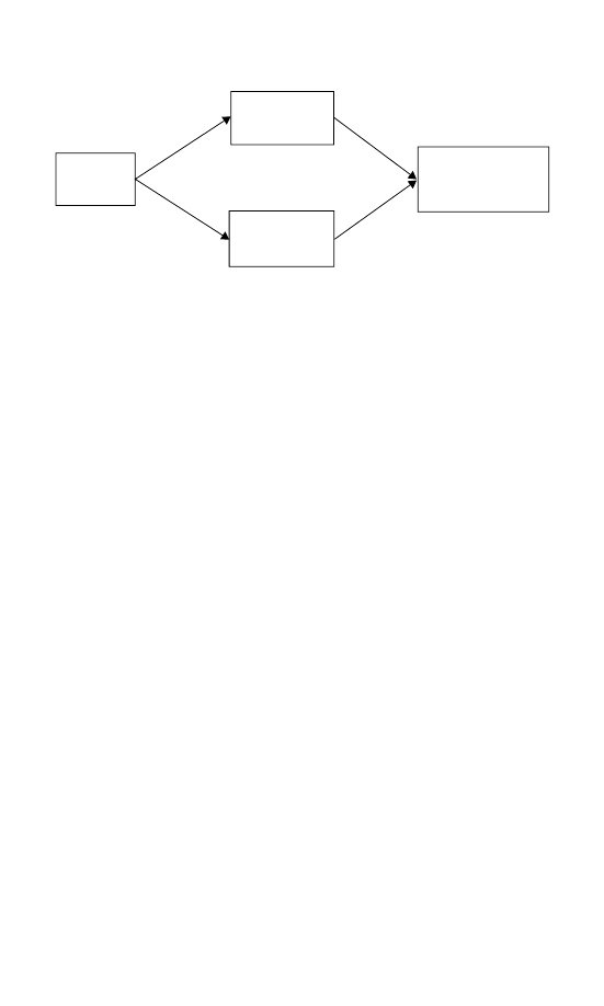
126
The Politics of Income Inequality in the United States
Public
Policy
Explicit
Redistribution
Market
Conditioning
Post-Government
Income
Distribution
figure 5.1. Policy and Two Mechanisms of Distributional Impact
conceptualizing and measuring macro policy:
micro vs. macro
To this point, I have often mentioned the term public policy but have
said little about how to define it. In this analysis, policy is concep-
tualized as the sum total of policies enacted by government. This
conceptualization has three important characteristics. First, it is only
interested in important and substantive change. Some activities by
policymakers represent failed policy attempts or symbolic activities
designed for an audience, but laws embody government policies that
at least have the potential to influence peoples’ lives. Second, policy is
viewed cumulatively – not as newly developed each year, but the result
of modifications to previous decisions. Changes occur at the margin
while most previous policy decisions remain in effect. These marginal
changes are what should influence the path of distributional outcomes.
Finally, this conceptualization of policy is highly aggregated. While it
is common to take a particularistic view of policy with each set of poli-
cies representing government’s response to a particular set of issues, a
focus on individual policies is not satisfying in the broader theoretical
context of the macro politics model.
My focus on policy at the macro level is what distinguishes it most
clearly from previous studies of public policy and distributional out-
comes, so I want to say a bit more about this aspect of the macro policy
concept. Traditionally, analysts interested in public policy divide pol-
icy into individual pieces or domains. Questions are framed in terms
of “does policy X influence outcome Y?” In the context of distribu-
tional outcomes, typical issues are the effect of transfer spending on

Macro Policy and Distributional Processes
127
distributional outcomes or the impact of welfare reform on income
inequality.
The concern with conceptualizing policy as an aggregate phe-
nomenon in the context of distributional outcomes is that such a con-
ceptualization might include policies unrelated to income inequality.
One hypothetical response to this concern might be to conceptualize
public policy at a more aggregate level than individual policies, but
not move to the highest level of aggregation. For example, this line of
thinking might lead to examining subsets of policy. One subset might
focus on policies that have distributional goals. A second subset might
focus on policies that do not. Arguably, conceptualizing such multiple
subsets of policy could even be used to generate measures of redistribu-
tional policy and market conditioning policy that are closely connected
to the mechanisms of distributional impact suggested by my applica-
tion of the macro politics model and power resources theory to income
inequality in the United States.
I have selected the more highly aggregated conception of public
policy for two primary reasons. First, the theory of distributional
outcomes that I have outlined argues that nearly every governmental
policy either redistributes income or conditions markets. I am agnos-
tic about which micro policies actually generate different distributional
outcomes, but the theory suggests that nearly all micro policies have the
potential to impact distributional outcomes via the market condition-
ing mechanism. One cannot fully ascertain the distributional impact
of government through the combination of redistribution and mar-
ket conditioning by examining just subsets of policy. Thus, the macro
policy conception is more consistent with the theory of distributional
outcomes that I have laid out and the macro politics model in general.
Second, examining the ideological tone of macro policy provides
an indicator of lower class power resources that would not be evident
with a more particularistic view of policy. Power resources theory often
thinks of micro policies as tools that those with power resources can
use to achieve desired outcomes. Left party control of government is
an indicator of lower class power resources, and left parties tweak
the tools of policy to change outcomes. Moving the conception of
policy to the macro level allows us to think of policy not just as a
set of individual tools that can change distributional outcomes, such
as transfer payments and job training, but as an indicator of power

128
The Politics of Income Inequality in the United States
resources in themselves. So, macro policy in one sense can be thought
of as a variable that intervenes between party control of government
and distributional outcomes. But the left-right content of macro policy
could be thought of as more than a mere intervening variable – it might
also be considered an additional and more precise indicator of lower
class power resources.
Macro policy as an indicator of power resources may be particularly
appropriate in the context of the United States. Despite the fact that
a connection between party control and distributional outcomes was
discovered in the analysis of the previous chapter, class-based interests
are not well-consolidated. While the Democratic Party is clearly more
oriented toward lower class interests than the Republican Party, class-
based partisan differences are not as clear in the United States as they
are in the European democracies where power resources theory has
been developed and typically tested. The reality of American politics is
that parties have been less disciplined (despite recent changes) and more
factionalized (often along regional lines) than most of their European
counterparts. In such a context, it seems unlikely that party control
is the best indicator of political power resources, and it increases the
utility of the macro policy concept.
With this aggregate conception of policy in mind, I use a measure
of policy developed by Erikson et al. (2002). This measure exam-
ines important policy change by focusing on the crucial public laws
identified by David Mayhew (2005). From this list, laws related to
domestic policy with national impact are coded as to whether they
were viewed as expanding (liberal) or contracting (conservative) gov-
ernment at the time they were passed. Laws that were ambiguous
in their expansion versus contraction of government were coded as
neutral and do not contribute to the policy change captured in this
measure. Liberal legislation is counted +1, conservative legislation
−1, and exceptionally important laws (as defined by Mayhew) are
counted +2 or
−2. Each year since 1947, a score is produced by
summing liberal minus conservative legislation – this is annual policy
change.
The current level of policy is produced by accumulating annual pol-
icy change over time. A net liberal shift in policy produces a positive
change in this policy measure. Since the late 1940s, the most important
policy changes have usually led to government expansion. In essence,
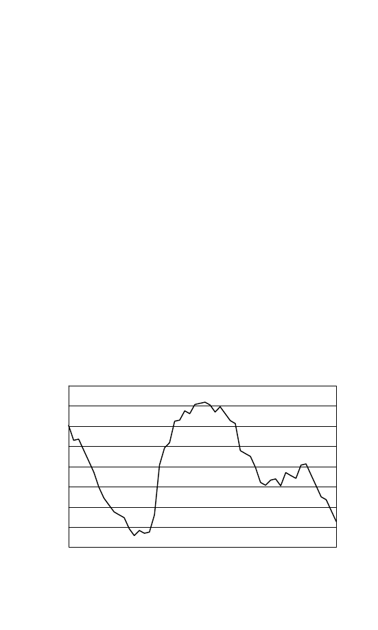
Macro Policy and Distributional Processes
129
then, the debate in the United States has not been literally about the
contraction versus expansion of government, but about how much
government should expand in response to the problems that develop
in an increasingly complex society. In the context of the post-World
War II United States, conservatives have not regularly offered propos-
als that would contract government. Rather, they have opposed new
government expansion. Given this, a measure that focuses simply on
the expansion versus contraction of government does not appropri-
ately capture policy as a result of the ideological conflicts occurring in
the governing system of the United States.
Since my interest is in determining which side of the ideological
debate is winning in political conflict, it is more appropriate to examine
the accumulation of policy relative to the long-term trend of govern-
ment expansion. During the period under analysis (1947–2000), there
was an average of 2.19 new laws passed each year that expanded
government activity. The detrended measure of policy utilized in this
analysis removes the trend of 2.19, rising only when the net increase
in government-expanding laws exceeds 2.19 and declining when the
net increase falls below 2.19. I will refer to this measure as policy lib-
eralism. It is charted in Figure 5.2 from 1947 to 2000 and shows that
the major turning points of policy occur in some expected places. A
–20
–15
–10
–5
0
5
10
15
20
1947 1951 1955 1959 1963 1967 1971 1975 1979 1983 1987 1991 1995 1999
P
o
licy li
b
e
ra
lis
m
figure 5.2. Policy Liberalism (Detrended), 1947–2000

130
The Politics of Income Inequality in the United States
sharp liberal turn in policy took place in the early 1960s as Lyndon
Johnson began his Great Society program, while policy turned in a
conservative direction around the time of Reagan’s election to the pres-
idency, and another sharp turn toward the right happened after the
Republican takeover of Congress in 1994.
policy and distributional outcomes, 1947–2000
The theoretical framework of this book suggests a particular set of
relationships between policy liberalism and distributional outcomes.
Liberal policy is expected to increase redistribution and decrease pre-
redistribution inequality, thereby decreasing overall inequality by def-
inition. With these expectations in mind, I conduct a time-series anal-
ysis of the connections between policy liberalism, pre-redistribution
inequality, and redistribution. The basic contours of the analysis are
similar to that conducted in the previous chapter. First, I extend
existing analyses of the political determinants of overt government
redistribution by examining the connection between policy liberalism
and redistribution. Then, I examine the relationship about which previ-
ous research has said the least – policy liberalism and pre-redistribution
inequality. This part of the analysis sheds light on whether market
conditioning influences income inequality. Throughout the analysis,
I again apply single equation error correction models (ECMs) to data
from 1947 to 2000.
Policy Liberalism and Government Redistribution
I found in the previous chapter that there is a direct link between the
party controlling the White House and the amount by which govern-
ment programs reduce inequality. While a variety of control variables
were included in initial models of government redistribution, in the
end only unemployment and the elderly population were linked to
government redistribution in addition to party control. Given knowl-
edge based on previous research that party control of policymaking
institutions is connected to the ideological tone of policymaking in
Washington (Erikson et al. 2002) and the close conceptual linkage
between party control and policymaking in the theoretical framework

Macro Policy and Distributional Processes
131
of my analysis, the final model of redistribution estimated in the previ-
ous chapter, with policy liberalism substituted for Democratic control
of the presidency, provides a useful framework for the analysis of policy
and redistribution.
3
Table 5.1 presents this model, which reports an ECM of changes in
redistribution regressed on lagged levels and current changes in unem-
ployment and the aged population, in addition to lagged levels and
changes in policy liberalism. This model answers two straightforward
questions. First, does policy liberalism increase government redistribu-
tion? Second, is the timing of the policy effect similar to that of party
control? The results support an affirmative answer to both questions.
table 5.1. Public Policy and Government
Redistribution,
1947–2000
Independent Variables
Redistribution
Error Correction Rate
−0.38
∗∗∗
(0.12)
Political Power Resources
Policy Liberalism
t
−1
0.01 (0.07)
Policy Liberalism
t
−1
0.05
∗∗
(0.02)
Labor Market Factors
% Unemployed
t
0.53
∗∗
(0.21)
% Unemployed
t
−1
0.57
∗
(0.29)
Demographic Factors
% Aged 65+
t
−1.56 (4.57)
% Aged 65
+
t
−1
2.93
∗∗∗
(0.94)
Response to Inequality
Pre-Redist. Inequality
t
4.94
∗∗∗
(0.72)
Constant
−14.32 (5.25)
Adj. R
2
0.77
N
52
Two-tailed significance levels:
∗∗
p
≤ 0.05;
∗∗∗
p
≤ 0.01.
Note: Table entries are time series regression coefficients
representing a single-equation error correction model
with standard errors in parentheses.
3
Estimating models with a wide variety of control variables included in the previous
chapter does not substantively change the results for policy liberalism reported here.
These more detailed results with all controls included are excluded because they are
parallel to those in the previous chapter and add nothing of substance to the simpler
results reported here.

132
The Politics of Income Inequality in the United States
As with party control, policy liberalism has a positive influence on
government redistribution that is distributed over time. A one point
positive shift in policy liberalism (an additional liberal law relative
to the long-term trend) produces no immediate impact on redistribu-
tion. However, this liberal shift does create a disequilibrium in which
redistribution is too low relative to policy liberalism. Beginning in the
year after the initial liberal shift, redistribution begins to respond by
increasing 0.05 points. In other words, a liberal shift in policy has
the short-term effect of increasing the percentage by which govern-
ment reduces inequality via explicit redistribution by 0.05 percentage
points. Substantively, this is a small impact, and even the long-run mul-
tiplier effect of a unit increase in policy liberalism on redistribution is
a mere 0.13 percentage point increase.
4
Still, this impact is consistent
with the predictions of power resources theory and the macro politics
model and, after all, is the impact of just one additional liberal law in
a given year. Thus, the importance of the connection between policy
and redistribution is real.
The results of the policy model are nearly identical to that of the
party control model estimated previously. Policy, like party control,
has an impact on redistribution that is distributed over time through
the error correction component. As in the party control model, unem-
ployment produces a positive and statistically significant increase in
redistribution in both the short and long term. The same is true for
the long-term impact of the aged population via the error correction
component. A one point increase in the percentage of the population
that is aged 65 and older increases redistribution by well over seven
points (2.93
/0.38 = 7.71). In this model, however, the aged popula-
tion has no short-term impact on redistribution. This is likely due to
the more nuanced measure of the ideological direction of government
action and lower class power resources utilized here. Change in con-
trol of the presidency can typically only occur every four years, whereas
policy liberalism can shift from year to year. This makes it less likely
that variables such as the aged population will make a difference for
redistribution in the short term. Still, the results here for party control
and policy liberalism are largely comparable.
4
A more in-depth discussion of the substantive size of policy impact on redistribution
occurs in the next chapter.

Macro Policy and Distributional Processes
133
Policy Liberalism and Pre-Redistribution Inequality
As with party control of government, the ideological tone of pol-
icy outputs directly affect government redistribution. Analyzing the
connection between policy liberalism and pre-redistribution inequal-
ity provides information about whether the effects of party control
and policy are also parallel with respect to the market conditioning
mechanism.
In Table 5.2, I present this analysis. As in the analysis of redistri-
bution, I begin with the final model of pre-redistribution inequality
estimated in the previous chapter, substituting policy liberalism for
party control of the presidency. In addition to policy liberalism as
an indicator of political power resources and union strength as an
indicator of market power resources, unemployment and immigration
are included as control variables. It is worth noting, however, that
including the wide variety of other controls that were considered in
the analysis of the previous chapter does not change the substance of
the reported results.
table 5.2. Public Policy and Pre-Redistribution Inequality,
1947–2000
Independent Variables
Pre-Redistribution Inequality
Error Correction Rate
−0.84
∗∗∗
(0.13)
Political Power Resources
Policy Liberalism
t
−1
−0.03
∗∗∗
(0.01)
Market Power Resources
% Unionized
t
−1
0.04 (0.06)
% Unionized
t
−1
−0.10
∗∗∗
(0.02)
Labor Market Factors
% Unemployed
t
−1
0.05 (0.03)
% Unemployed
t
−1
0.10
∗∗∗
(0.02)
Demographic Factors
% New Immigrants
t
−1
−0.84
∗∗∗
(0.21)
% New Immigrants
t
−1
0.57
∗∗∗
(0.18)
Adj. R
2
0.54
N
52
Two-tailed significance levels:
∗
p
≤ 0.10;
∗∗
p
≤ 0.05;
∗∗∗
p
≤ 0.01.
Note: Table entries are time series regression coefficients representing a
single-equation error correction model with standard errors in parentheses.

134
The Politics of Income Inequality in the United States
The results reported in Table 5.2 are unequivocal. Policy liberalism
and union strength, the variables of central theoretical interest, have
significant effects on income inequality. Liberal shifts in public pol-
icy produce reductions in pre-redistribution inequality, as does union
strength. Substantively, a one point increase in policy liberalism (i.e.,
the average number liberal laws passed each year is exceeded by one,
representing a 1 percent change based on the variance of this series)
reduces the ratio of the aggregate income of the top income quintile
to the bottom two quintiles by 0.03 points. This amounts to approxi-
mately a 2.5 percent change. So, a 1 percent increase in policy liberalism
produces a 3 percent reduction in inequality. This is a substantively
important impact, and given the nonstationarity of pre-redistribution
inequality in terms of its time series properties, this influence of policy
leads to a permanent change in distributional outcomes. That is, once
inequality increases or decreases in response to a change in policy, that
increase or decrease continues into the future until some countervail-
ing force emerges. Importantly, since the dependent variable in this
analysis captures inequality that exists prior to the explicit effects of
government redistribution, this shows that market conditioning is an
avenue through which policy influences distributional outcomes. While
government overtly uses transfer policies to change the income distribu-
tion, policy also influences inequality before explicit transfers. In addi-
tion, the distributional consequences of policy via market conditioning
are felt quickly since the policy effect is fully captured in the short term.
conclusion
Previous theoretical development of the macro politics model has
focused on a variety of macro-social phenomena in the United States.
Income inequality, however, has not been previously analyzed as a
component of the U.S. macro polity. Instead, the policies produced by
the U.S. national government are essentially analyzed as the final prod-
uct of the political process. In this chapter I linked insights from power
resources theory and the macro politics model to generate expecta-
tions about the connection between the ideological direction of policy
outputs and distributional outcomes.
The central question of this chapter was whether policy liberalism
reduces income inequality via redistribution and/or market condition-
ing. The answer is yes on both counts. When public policy shifts toward

Macro Policy and Distributional Processes
135
the left, the most immediate effect is a reduction in pre-redistribution
inequality – the distribution of income produced primarily by decisions
made in more or less open markets. Market decision makers observe
a shift in policy and quickly change their behavior to adapt to the
new reality of government policy. But this is not the only distribu-
tional consequence for a change in public policy. A shift to the left in
policy also creates a disequilibrium in which redistribution is too low
when compared to the ideological tone of policy. At the rate of about
38 percent each year after the policy shock, redistribution increases
to catch up with policy, eventually increasing government redistribu-
tion by 0.13 percentage points for every new liberal law (relative to
the trend) enacted. Interestingly, the effect of policy liberalism on pre-
redistribution inequality occurs more quickly than its effect on explicit
redistribution. This means that the explicit redistributive impact of gov-
ernment is slower to respond to macro political change than is the more
nebulous impact that the state achieves through market conditioning.
While the analysis in this chapter answered many questions, there
are still a few matters that remain unresolved. Is it possible that pre-
redistribution inequality responds to redistribution, thus generating
a form of reciprocal causation that has not been accounted for in the
analysis to this point? Are there indirect effects of politics on inequality
that manifest themselves via the labor market? What is the overall sub-
stantive impact of politics on the distribution of income in the United
States? I turn to these issues in the next chapter.

6
Putting the Pieces Together: Who Gets
What and How
The previous two chapters tested the central predictions of power
resources theory and the macro politics model for distributional out-
comes in the United States. Chapter 4 demonstrated that Democratic
control of the presidency is associated with lower levels of income
inequality, and this is the case because explicit redistribution is greater
and market inequality is lower when a Democrat is in the White House
as opposed to a Republican. This is consistent with the main predic-
tions of power resources theory and my extension of it to the U.S. case.
Chapter 5 focused on public policy as a central variable in the macro
politics model and assessed whether leftward shifts in macro policy pro-
duce reductions in inequality. The evidence supported the conclusion
that the macro politics model can be extended to distributional out-
comes. Like Democratic Party control, public policy liberalism reduces
inequality via both market conditioning and explicit redistribution.
The models examined in the previous two chapters are depicted in
the form of a path model in Figure 6.1. The light solid lines are the paths
analyzed in both Chapters 4 and 5. The heavy dotted lines represent
paths examined in Chapter 4 alone, and the heavy solid lines are the
paths examined in Chapter 5 alone. The essential item to note from
this diagram is that the analysis to this point has treated all explanatory
factors as influencing distributional outcomes in a single causal stage.
These models are interesting and provide clear evidence in support of a
combination of power resources theory and the macro politics model.
But when added together they are more than the sum of their parts.
136
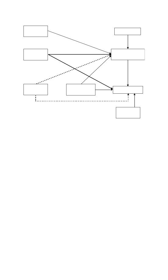
Who Gets What and How
137
Union
Strength
Policy
Liberalism
Democratic
President
Unemployment
Rate
Redistribution
Aged
Population
Immigration
Pre-Redistribution
Inequality
figure 6.1. A Depiction of the Models Examined in Chapters 4 and 5
In this chapter, I combine these previous models in order to answer
questions about the distributional process that have been unexplored
in the analysis to this point.
a more complete picture of politics and income
inequality
The strategy of modeling all explanatory variables in a single causal
stage is an appropriate way to determine the direct effects of politi-
cal factors on distributional outcomes, but this likely fails to capture
fully and accurately the overall impact of politics on the distributional
process. Specifically, this approach leaves three important unan-
swered questions. First, while it is clear that macro political dynamics
have clear and direct effects on distributional outcomes, examining
the effect of politics in a single stage leaves open the question of
whether political variables have indirect effects via their influence
on other explanatory factors. An indirect effect might occur, for
example, if Democrats reduce unemployment, which in turn reduces
pre-redistribution inequality. The second remaining question is related
to the linkages between pre-redistribution inequality and redistribution

138
The Politics of Income Inequality in the United States
– how does pre-redistribution inequality respond to explicit redistri-
bution? While pre-redistribution inequality was included as a control
variable in models of redistribution, the potential effect of redistribu-
tion on pre-redistribution inequality has not been examined. Third,
the analysis has focused only on explanatory factors hypothesized to
have a direct impact on income inequality. In the context of the macro
politics model, it is important to learn whether or not distributional
outcomes are responsive to changes in mass preferences. If a change in
public opinion can be linked to distributional outcomes, this effect will
be indirect, coming via representational mechanisms that influence the
composition of government and public policy.
Indirect Effects of Politics via Employment Policies
The models in Chapters 4 and 5 examine the direct impact of the theo-
retically central variables while controlling for potentially confounding
factors. For example, in Chapter 4, the effects of union strength
and party control of government (power resources variables) on pre-
redistribution inequality were estimated while controlling for labor
market and demographic factors. This type of analysis is useful for
determining whether power resources and macro politics variables are
directly linked to distributional outcomes while controlling for other
potential explanations. The results to this point demonstrate that such
a direct link does, in fact, exist between politics and distributional out-
comes. Along with the controls for unemployment, pre-redistribution
inequality, and the aged population, party control of government and
policy liberalism have an impact on redistribution. Similarly, the cen-
tral theoretical variables of party control, policy liberalism, and union
strength are directly connected to pre-redistribution inequality while
controlling for economic and demographic factors.
Thus far, the analysis leads to the conclusion that party control
and public policy have an influence on inequality via both market
conditioning and redistribution, but there is no basis on which to
make a judgment regarding the overall impact of politics on dis-
tributional outcomes. The approach of the previous two chapters
estimates only the direct impact of politics on redistribution and pre-
redistribution inequality, but not necessarily the total impact. The
total impact could be identical to the direct impact, but this would

Who Gets What and How
139
require an important assumption – namely, that the political variables
having a direct impact on distributional outcomes do not also influence
other explanatory variables. This assumption is almost certainly incor-
rect with respect to unemployment. Numerous previous studies have
found that party control of government influences unemployment rates
(Alesina and Rosenthal 1995, Erikson et al. 2002, Hibbs 1987, Hibbs
and Dennis 1988). The analysis to this point, however, does not
explore what impact political factors have on income inequality via
this indirect causal path.
Thus, the first complication that I introduce in this chapter is the
consideration of indirect political effects via unemployment. Rather
than treating unemployment like other control variables, it will be
treated as an endogenous variable that not only explains distributional
outcomes, but also is explained by politics. This will provide a basis
to estimate any additional impact that political variables have via their
influence on unemployment. Based on previous research, the expecta-
tion is that Democratic control of government and policy liberalism
decrease unemployment. Given that reductions in unemployment
decrease pre-redistribution inequality, the indirect impact of politi-
cal factors should augment their direct equalizing impact via market
conditioning. The indirect impact of political factors on redistribu-
tion, however, should moderate their direct impact, since any reduced
unemployment generated by Democratic control or policy liberalism
would reduce redistribution. This would counteract the increase in
redistribution that is produced by the direct effect of these variables.
Linkages Between Redistribution and Pre-Redistribution Inequality
A second issue that has not been fully addressed in Chapters 4 and
5 is the connection between pre-redistribution inequality and redistri-
bution. In my models of redistribution, I included pre-redistribution
inequality as a control variable based on the idea that higher levels of
existing inequality will induce more redistributive effort to narrow the
gap between the top and the bottom of the income distribution. This is
in line with recent studies of redistribution (Bradley et al. 2003) as well
as the classic political economy model of Meltzer and Richard (1981).
These earlier results showed that the impact of pre-redistribution
inequality on redistribution is strong and positive. This in and of itself

140
The Politics of Income Inequality in the United States
indicates the existence of an indirect path (in addition to that via
unemployment discussed above) between political factors and redis-
tribution. That is, we know that power resources and macro politics
variables are directly connected to pre-redistribution inequality. Demo-
cratic control of the presidency and leftward shifts in policy reduce
pre-redistribution inequality. Furthermore, the models in the two pre-
vious chapters show that this reduction in pre-redistribution inequality,
in turn, reduces redistribution. Thus, there is an indirect path between
political factors and redistribution. This indirect path should be
considered alongside the indirect effects that occur via unemployment.
While the impact of pre-redistribution inequality on redistribution
was considered in the earlier analysis, the potential reverse connection
was not explored. That is, I have not yet considered the possibility that
redistribution increases pre-redistribution inequality. The main reason
that this possibility has not been considered to this point is that the
comparative evidence argues against such a connection. Most recently,
Bradley et al. (2003) provided direct evidence on this point when they
found no connection between welfare state generosity and pretax and
transfer inequality. Despite the existing comparative evidence, how-
ever, it is important to consider the possibility that redistribution
influences pre-redistribution inequality in the context of the liberal U.S.
welfare state. Furthermore, unintended effects of redistribution on pre-
redistribution inequality may eliminate any gains in equality produced
by left parties and policies if more redistribution results in increases in
market inequality.
Critics of the welfare state and some public economists have made
this argument explicit. Browning (2002) discusses seven general argu-
ments against redistribution, and three of these arguments are related
to the idea that those at the bottom of the income distribution are
made worse off by redistribution. One of the main mechanisms by
which redistribution might increase pre-redistribution inequality is via
work effort. Basic microeconomic theory predicts that providing some-
one with a transfer payment will produce a reduction in their private
labor market effort. Thus, the benefits to a poor individual of a redis-
tributive government benefit will be at least partially offset by reduced
work effort. Several economic studies have found evidence consistent
with this reduced work effort hypothesis in the United States (Danziger
et al. 1981, Moffitt 1992). However, these studies do not directly
examine the impact of redistribution on market income inequality.

Who Gets What and How
141
Thus, accounting for the possibility of a two-way relationship between
redistribution and pre-redistribution inequality will provide not only
a more accurate assessment of power resources theory and the macro
politics model, but will also provide new evidence related to economic
theories of distributional outcomes.
Macro Politics and the Public Mood
The third and final question left unanswered by the approach utilized
in the previous two chapters relates to the role of public opinion in
the macro politics model. The previous models were concerned only
with estimating the impact of variables that have a direct effect on the
dependent variable. A group of independent variables are inserted on
the right-hand side of a regression equation, and those with signifi-
cant coefficients are interpreted as influencing the dependent variable
while statistically controlling for all the other independent variables.
At times, however, there are variables of theoretical interest that have
no direct effect on the outcome variable that may have only an indirect
influence via their effect on other factors that do have a direct impact.
This is precisely the situation that may be present with regard to the
macro politics model and distributional outcomes. As discussed earlier,
previous work in the macro politics tradition has been primarily con-
cerned with public policy as the outcome of the governing system. One
of the goals of my work, of course, is to extend the macro politics model
to distributional outcomes by examining the connection between pol-
icy and income inequality. The analysis in Chapter 5 accomplished just
that. However, one of the most interesting and important implications
of extending the macro politics model to distributional outcomes has
not been assessed – does the public mood influence societal outcomes?
When earlier macro politics research is combined with my anal-
ysis, it appears likely that changes in public opinion produce an
indirect impact on distributional outcomes. If shifts to the left in
the public mood produce Democratic control of government and left
policymaking, and these political variables in turn produce greater
pre-redistribution equality and more government redistribution, then
(at least indirectly) shifts to the left (or right) in public opinion
produce lower (or higher) levels of income inequality. If true, this
would be a fascinating finding with important implications for recent
examinations of inequality and American democracy (Bartels 2006,

142
The Politics of Income Inequality in the United States
2008, Weissburg 2006). The third extension to the analysis that I will
implement in this chapter, then, is an explicit consideration of public
opinion as an indirect influence on distributional outcomes.
the comprehensive model: a simultaneous
equation approach
The unexplored questions discussed to this point motivate three exten-
sions to the previous analysis. First, the indirect effects of party control
and public policy will be assessed by providing a more careful spec-
ification of the causal ordering of the explanatory variables. More
specifically, I consider unemployment as a variable which not only
affects distributional outcomes directly, but is also an intervening vari-
able that creates additional causal paths for the impact of political
power resources on redistribution and market inequality. In addition,
I treat party control of government as causally prior to public policy
rather than entering the model at the same stage. This is consistent
with macro politics findings showing that party control is a determi-
nant of public policy (Erikson et al. 2002). Second, the possibility of
a two-way connection between redistribution and pre-redistribution
inequality is examined. This provides a more appropriate estimate of
the connection between these two variables, and also opens the possi-
bility for further indirect causal paths between union strength, party
control, public policy, and distributional outcomes. Third, I include a
measure of aggregate public opinion as a determinant of party control
and public policy to test the ability of changes in mass preferences to
influence important economic outcomes.
Figure 6.2 depicts this final model that I examine in this chapter.
This figure is arranged in a similar fashion to the earlier Figure 6.1,
with the exception that public mood is added here. The heavier lines
indicate connections that were not included in the earlier analysis, and
the subscripts indicate the temporal arrangement of the variables. It is
also useful to note that Figure 6.2 is a spatially rearranged depiction
of the theoretical model originally outlined at the beginning of the
book in Figure 1.8, with important economic and demographic control
variables added here.
Two of the three wrinkles that I add to the analysis in this chapter are
essentially about specification of causal ordering – namely considering
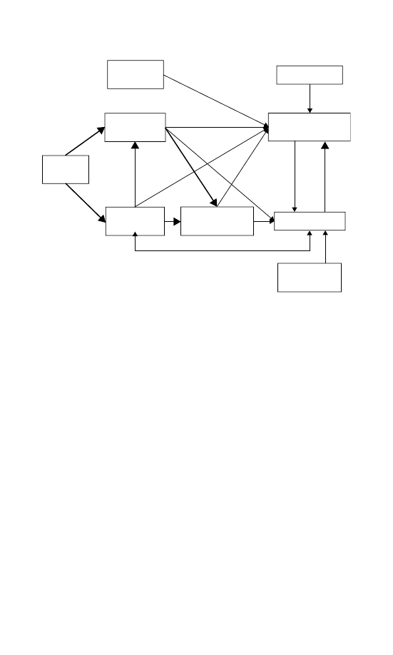
Who Gets What and How
143
Union
Strength
t–1
Immigration
t–1
Pre-Redistribution
Inequality
t
Redistribution
t
Aged
Population
t
Unemployment
Rate
t
Democratic
President
t–1
Public
Mood
t–2
Policy
Liberalism
t–1
figure 6.2. A Path Model of Macro Politics, Power Resources, and Distri-
butional Outcomes (heavy lines indicate paths added to the analysis in this
chapter)
both the direct and indirect effects of party control and policy and
adding public mood to the model in order to assess its indirect effect
on distributional outcomes. Using the impact of party control on pre-
redistribution inequality as an example helps to illustrate the idea of
direct and indirect effects. Each arrow in Figure 6.2 represents the
impact of one variable on another. There is an arrow, for example, that
runs from “Democratic President” to “Pre-Redistribution Inequality.”
This is a direct effect, because the path of the arrow is not interrupted by
other variables. There is also an indirect path (this path is only hypoth-
esized at this point) between party control and pre-redistribution
inequality that runs through unemployment, which would be called an
intervening variable. This is the case because an arrow runs not only
between “Democratic President” and “Unemployment,” but also from
“Unemployment” to “Pre-Redistribution Inequality.” Indirect effects
occur whenever there is a path linking one variable to another and this
path is interrupted by other intervening variables. One can see several
potential indirect effects hypothesized in Figure 6.2.

144
The Politics of Income Inequality in the United States
Through statistical analysis, it is possible to calculate the magnitude
of these direct and indirect effects, which can then be combined to
calculate total effects. The introduction of direct and indirect effects
to the model does not fundamentally alter the econometric techniques
applied. Accounting for the direct and indirect effects of a variable
simply requires additional error correction models (ECMs) estimated
in the usual way. Continuing with the example of the impact of party
control on pre-redistribution inequality, the direct effect of policy could
be estimated in just one ECM like this:
Pre
t
= α
0
+ α
1
Pre
t
−1
+ β
0
DemPres
t
−1
+ β
1
DemPres
t
−1
+ β
2
Unemp
t
+ β
3
Unemp
t
−1
+
t
(6.1)
This, in fact, is a simplified version of a model taken directly from
Chapter 4, with the difference being that union strength and immigra-
tion are dropped here for the sake of simplicity. The direct effect of
Democratic control of the presidency on pre-redistribution inequality
could be computed by the short-term (
β
0
) or long-term (
β
1
/α
1
) impact
of party control. But if we wish to examine the potential indirect effect
of party control via unemployment, a further model must be estimated:
Unemp
t
= γ
0
+ γ
1
Unemp
t
−1
+ λ
0
DemPres
t
−1
+ λ
1
DemPres
t
−1
+ ρ
t
(6.2)
If party control is found to have a significant influence on unem-
ployment, then the indirect effect of party control on inequality via
unemployment could be calculated by multiplying the effect of party
control on unemployment by the effect of unemployment on pre-
redistribution inequality.
1
The total effect, then, could be determined
by summing the direct and indirect effects.
Much of the model depicted in Figure 6.2 could be estimated via
a series of error correction models for each of the endogenous vari-
ables: pre-redistribution inequality, redistribution, unemployment,
1
Path coefficients are traditionally presented as standardized effects when calculating
direct and indirect effects. It is a simple matter to switch between standardized and
unstandardized effects. Standardized coefficients can be computed from unstandard-
ized coefficients as follows:
β
s
= β
u
∗ σ
x
/σ
y
, where
σ
x
and
σ
y
refer to the standard
deviation of the explanatory and outcome variables, respectively.

Who Gets What and How
145
and policy liberalism. However, the more complex model assessed
in this chapter does require a few modifications to these economet-
ric methods because of the two-way causation hypothesized between
redistribution and pre-redistribution inequality. More technically,
since reciprocal causation is hypothesized between redistribution and
pre-redistribution inequality, any regression of redistribution on pre-
redistribution inequality and vice-versa could produce biased param-
eter estimates due to correlation between the error term and an
explanatory variable. To overcome this problem, I estimate a system
of error correction equations based on the above path diagram utiliz-
ing three-stage least squares. Using three-stage least squares resolves
the bias introduced by reciprocal causation between redistribution and
pre-redistribution inequality and provides for appropriate estimates of
the direct and indirect effects of power resources and macro politics
variables. However, application of this estimation procedure in no
way limits my ability to account for the time dynamics present in the
data. I am simply re-estimating the models of the previous two chapters
using procedures that account for both time dynamics and potential
reciprocal causation.
Using the results of the earlier chapters as a guide to determine
which explanatory variables to include for each dependent variable,
the system of equations that I estimate via three-stage least squares is
as follows:
2
Y
1
= α
0
+ α
1
Y
1
+ β
0
Y
2
+ β
1
Y
3
+ β
2
Y
3
+ β
3
X
3
+ β
4
X
3
+ β
5
X
2
+ β
6
X
2
+ β
7
X
5
+ β
8
X
6
+
1
(6.3)
2
Policy liberalism was initially included as an explanation of unemployment, but was
found to be insignificant and was dropped from the analysis. The equations below
do not include a path from policy to unemployment in order to avoid additional
complexity. As in any simultaneous equation model, it is important to discuss the
identification of the model. Identification refers to the question of whether there is
enough information in the data analyzed to estimate the unknown quantities in the
model. If a model is not identified then it cannot be estimated properly. Oftentimes
it is straightforward to see that a set of simultaneous equations is identified, but in
models with such a large number of coefficients and reciprocal paths, identification is
not so obvious. In an identified model, each equation has at least as many exogenous
variables (those that do not appear on the left-hand side of any equation) excluded
on the right-hand side as it has endogenous variables (those that appear on the left-
hand side of any equation in the system) included on the right-hand side. Only the

146
The Politics of Income Inequality in the United States
Y
2
= α
2
+ α
3
Y
2
+ β
9
Y
1
+ β
10
X
4
+ β
11
X
4
+ β
12
Y
3
+ β
13
Y
3
+ β
14
X
5
+ β
15
X
5
+ β
16
X
6
+ β
17
X
6
+
2
(6.4)
Y
3
= α
4
+ α
5
Y
3
+ β
18
X
5
+ β
19
X
5
+
3
(6.5)
In addition, to examine the paths between public mood, party control,
and policy, I estimate the following equations separately using standard
time series techniques since these dependent variables are fully exoge-
nous to the system above and need not be included in the three-stage
least squares estimation:
3
X
5
= α
6
+ α
7
X
5
+ β
20
X
1
+ β
21
X
1
+
4
(6.6)
X
6
= α
8
+ α
9
X
6
+ β
22
X
5
+ β
23
X
1
+
5
(6.7)
where, for all equations:
Y
1
= Pre-Redistribution Inequality
t
Y
2
= Redistribution
t
Y
3
= Unemployment
t
X
1
= Public Mood Liberalism
t
−2
X
2
= Union Strength
t
−1
first two equations in the system estimated here include endogenous variables on the
right-hand side. In the first equation, two endogenous variables (
Y
2
and
Y
3
) are
included on the right-hand side (lagged levels are considered pre-determined since
they only appear on the right-hand side) and four exogenous variables are excluded
(
X
4
, X
4
, X
5
, and X
6
). This equation is identified. The second equation also includes
two endogenous variables on the right-hand side (
Y
1
and
Y
3
) and excludes four
exogenous variables (
X
3
, X
3
,
X
4
, and Y
4
), thus also being identified and rendering
the system as a whole identified as well.
3
These specifications largely mimic those examined by Erikson et al. (2002), with the
exception that their analysis examined election outcomes as the Democratic vote share
while I examine the outcome as a dichotomy. Though these equations are both esti-
mated using standard time series OLS, the results can be reproduced in substance by
utilizing either logit or probit to estimate the results for party control. I present the
OLS results for ease of presentation, given that discussing logit or probit results in the
context of a path analysis would greatly limit substantive interpretation. Regardless,
only the discussion of the impact of the public mood could be influenced by this sim-
plification. Given the largely parallel substantive results using logit and probit, any
impact on this discussion is a matter of degree rather than kind.

Who Gets What and How
147
X
3
= Immigration
t
−1
X
4
= Aged Population
t
X
5
= Democratic President
t
−1
X
6
= Policy Liberalism
t
−1
This is a complicated set of equations, but they are essentially a
mathematical representation of the diagram presented in Figure 6.2.
Each of the equations above has a dependent variable on the left side
of the equation and a series of explanatory variables on the right side.
The dependent variables are simply those from Figure 6.2 that have
arrows pointing toward them, and the independent variables are those
from the figure that have arrows running away from them. The model
itself is simply a combination of the models in Chapters 4 and 5 with a
couple of straightforward additions (public mood and a path between
party control and policy liberalism) that spring directly from previous
studies in the macro politics tradition.
Results
While I will not go into great detail here about the specifics of three-
stage least squares estimates since the primary purpose of this analysis
is simply to provide the basis for calculating the total impact of political
dynamics on distributional outcomes (which will be discussed below),
it is encouraging to note that the first two columns of Table 6.1 in large
part mirror the models of redistribution and pre-redistribution inequal-
ity analyzed in the previous two chapters. The coefficient estimates in
the second column for redistribution, in fact, are nearly identical to
those from Chapters 4 and 5. The direct effect of both Democratic con-
trol and left public policy is an increase in redistribution via the error
correction mechanism. In fact, the only difference between this model
and the one discussed in the previous chapters is that these coefficient
estimates are actually slightly larger, though substantively similar. The
model of pre-redistribution inequality reported in Column 1 also tells a
story similar to that of Chapters 4 and 5. Lower class power resources
and leftward shifts in macro political factors produce a direct effect
of lower levels of pre-redistribution inequality. However, the coeffi-
cient estimates of the three-stage least squares model reported here are

148
The Politics of Income Inequality in the United States
table 6.1. Estimating a Structural Model of Distributional Outcomes
Independent Variables
(1)
(2)
(3)
(4)
(5)
Error Correction Rate
−0.37
∗∗∗
−0.41
∗∗∗
−0.26
∗∗∗
n.a.
−0.25
∗∗
(0.10)
(0.12)
(0.14)
(0.10)
Democratic President
t
−1
−0.17
∗∗∗
−0.36
−0.97
∗∗
2.07
∗
−0.30
∗∗∗
(0.06)
(0.67)
(0.41)
(1.13)
(0.09)
Democratic President
t
−1
1.22
∗∗∗
−0.54
∗
0.40
(0.29)
Policy Liberalism
t
−1
−0.01
∗∗
0.06
(−0.006)
(0.06)
Policy Liberalism
t
−1
0.04
∗
(0.02)
% Unionized
t
−1
0.02
(0.03)
% Unionized
t
−1
−0.05
∗∗∗
(0.01)
% Unemployed
t
0.00
0.77
∗∗∗
(0.02)
(0.21)
% Unemployed
t
−1
0.07
∗∗∗
0.78
∗∗
(0.02)
(0.31)
% Aged 65+
t
1.77
(3.79)
% Aged 65
+
t
−1
3.21
∗∗∗
(0.98)
% Immigrants
t
−1
−0.49
∗∗∗
(0.11)
% Immigrants
t
−1
0.29
∗∗∗
(0.09)
Public Mood
t
0.01
(0.02)
Public Mood
t
−1
0.20
∗∗
0.02
∗
(0.09)
(0.01)
Pre-Redist
t
4.65
∗∗∗
(0.90)
Redist
t
0.08
∗∗
(0.01)
Constant
2.09
∗∗∗
−17.70
∗∗∗
1.71
∗∗∗
−12.15
∗∗
−1.16
∗
(0.70)
(5.85)
(0.60)
(5.18)
(0.66)
R
2
0.86
0.82
0.33
0.20
0.20
N
52
52
52
48
48
Two-tailed significance levels:
∗
p
≤ 0.10;
∗∗
p
≤ 0.05;
∗∗∗
p
≤ 0.01.
Note: Dependent variables by column are as follows: (1)
Pre-Redistribution Inequal-
ity, (2)
Redistribution, (3) Unemployment, (4) Policy Liberalism, and (5)
Democratic President. The first three columns report three-stage least squares coefficients
representing single-equation error correction models with standard errors in parentheses.
The final two columns report time series regression coefficients with standard errors in
parentheses. Public mood (liberalism) is first available in 1952, limiting the number of
years to 48 for models including public mood.

Who Gets What and How
149
slightly smaller than those in the previous analysis. This makes sense
given that an additional control for the amount of redistribution is
added to the model here.
The third column of the table presents the results for unemployment,
which were also estimated as part of the three-stage least squares sys-
tem of equations. Consistent with previous studies, Democratic control
of the White House decreases unemployment. Public policy, however,
has no direct effect on unemployment independent of party control
and is therefore dropped from the model. The last two columns of
the table assess the effect of Stimson’s (1999) public mood liberalism
measure on party control of the presidency and policy liberalism. Lib-
eral shifts in public opinion increase the likelihood of a Democratic
presidency and increase the liberalism of public policy. These results
indicate that public opinion has an indirect impact on distributional
outcomes. The results also show that macro political factors have indi-
rect paths of influence on distributional outcomes as well as a direct
influence.
Perhaps the most interesting result in Table 6.1 is that we
observe a reciprocal relationship between redistribution and pre-
redistribution inequality. As we saw in the previous chapters, higher
pre-redistribution inequality produces an increase in redistribution.
This is evidenced by the model in Column 2, in which a one-unit
change in pre-redistribution inequality produces an increase of 4.65
in redistribution. So, if the ratio of the income of the top income quin-
tile to the bottom two income quintiles increases by one, the percentage
reduction in inequality attributable to the first-order effects of explicit
redistribution increases by more than 4.5 percentage points. This effect
is likely due to the fact that when inequality goes up, eligibility for
redistributive programs goes up at the same time. It would be inappro-
priate, however, to conclude that the link between pre-redistribution
inequality and redistribution is merely due to economic downturns,
for this connection remains even while controlling for business cycle
indicators such as unemployment (and GDP and a variety of other
indicators not shown in the analysis here). We must keep in mind that
relative economic conditions indicated by income inequality are dis-
tinguishable from absolute economic outcomes like median income,
unemployment, and GDP. For example, if the gap between the rich
and poor is increasing dramatically it is possible for general economic

150
The Politics of Income Inequality in the United States
indicators to be improving while, at the same time, there are more
poor people eligible for means-tested programs. A second mechanism
that might be at work here is public opinion. Voters may respond to
increased inequality by demanding more redistribution, shifting their
mood to the left, electing more Democrats, and pressuring even Repub-
licans to provide more generous benefits. This is precisely the argument
put forward by Meltzer and Richard (1981).
What is new here is that, consistent with microeconomic theory, the
reverse is also true – redistribution conditions market outcomes, with
greater redistributive impact by government pushing pre-redistribution
inequality higher. More specifically, we see in Column 1 of the table
that when redistribution increases by a full percentage point, pre-
redistribution inequality is increased by 0.08 points. Remembering that
the average change in pre-redistribution inequality is 0.22 points, this
is a notable impact confirming that increasing redistribution can have
unintended and undesirable side-effects.
These results have an important implication for what happens when
a leftward shift occurs in the macro polity – that is, when a Demo-
crat takes over the White House or policy liberalism increases. We
know that such leftward shifts have the direct impact of reducing
pre-redistribution inequality and increasing redistribution. Interest-
ingly, though, these reductions in pre-redistribution inequality are
partly offset by simultaneous increases in pre-redistribution inequal-
ity that are spawned indirectly by the increased redistribution. By the
same token, these direct increases in redistribution can be reduced
by the simultaneous reductions in redistribution generated indirectly
by decreases in pre-redistribution inequality. Given these possibilities
and the results from the models of unemployment, party control, and
public policy, it is important to fully consider the direct and indirect
impact of politics on redistribution and pre-redistribution inequality,
as well as the overall impact of these variables on post government
inequality.
In order to facilitate the calculation of the direct and indirect
impact of macro politics, lower class power resources, labor mar-
ket, and demographic factors, I present a path diagram of the full
structural model in Figure 6.3. On each path I display the standard-
ized combined short and long-term impact of the explanatory variable
on the dependent variable, based on the coefficient estimates from
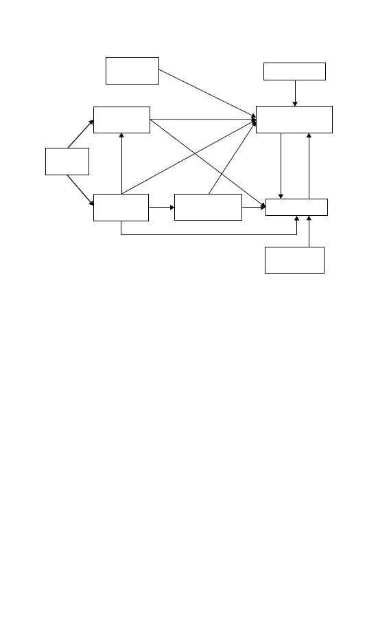
Who Gets What and How
151
Union
Strength
t–1
Policy
Liberalism
t–1
Public
Mood
t–2
Democratic
President
t–1
Unemployment
Rate
t
Redistribution
t
Aged
Population
t
0.856
0.232
0.356
0.089
0.760
0.104
.267
0.061
–0.750
–0.127
–0.076
1.02
0.103
–0.679
0.203
Immigration
t–1
Pre-Redistribution
Inequality
t
figure 6.3. Path Diagram for Full Model, Standardized Short- and Long-
Term Impact
Table 6.1. Insignificant coefficients are excluded from the diagram. For
some paths, such as that between party control and pre-redistribution
inequality, only a short-term impact is present. For others, like the
path between union strength and pre-redistribution inequality, only
an effect via the error correction component is present. In still other
cases, like the impact of unemployment on redistribution, both short-
and long-term effects are present. In all cases in which long-term effects
are present, the long-term effect is the standardized effect that would
be realized after the error correction is complete.
Comparing the Magnitude of Direct Effects
In the next section, I use these path coefficients to calculate the total
effects of the explanatory variables on distributional outcomes. At
this point, however, I want to focus on comparing the magnitude
of the direct effects presented in the figure. Comparing the variables
that directly influence redistribution, we find that the aged popula-
tion is by far the strongest predictor, with an effect that is more

152
The Politics of Income Inequality in the United States
than twice as large as the second most important explanatory factor,
pre-redistribution inequality. Of the variables that are of central the-
oretical interest, both party control and policy have important direct
effects on redistribution. However, their direct effects are small in com-
parison to factors such as unemployment and the aged population.
Much of the effect of these political variables on redistribution occurs
via indirect paths, and the indirect paths in most cases work against the
direct effects. For example, the direct impact of a Democratic president
on redistribution is positive. However, the indirect effect via unemploy-
ment is negative since Democratic presidents decrease unemployment
which, in turn, decreases redistribution.
Switching focus to pre-redistribution inequality, we again see that
party control and policy have direct effects that are much smaller than
unemployment. As well, compared to the direct effect of immigration
on pre-distribution inequality, the effect of party control is just one-
third as large and the impact of policy liberalism is approximately half
as large. In addition, many of the indirect effects of party control and
public policy actually augment their direct effect. For example, the
direct effect of Democratic control is
−0.076, which is augmented by
its indirect effect via unemployment. While redistribution has the sin-
gle largest direct impact on pre-redistribution inequality, market power
resources as indicated by union strength have the second largest impact.
All in all, lower class power resources and macro politics are impor-
tant predictors of both pre-redistribution inequality and redistribution,
but the results are actually somewhat stronger for pre-redistribution
inequality than redistribution. This again supports the conclusion
that politics influences distributional outcomes more via the market
conditioning mechanism than via redistribution in the United States.
Comparing the Magnitude of Total Effects
Even more useful than comparisons of the direct effects of the explana-
tory variables is a calculation of the total effects produced by the
combined direct and indirect impact of each variable. These total
effects are calculated for each explanatory variable in Table 6.2. The
first column of the table reports the standardized and unstandardized
total effect of each variable on pre-redistribution inequality, while
the second column reports the same information for redistribution.

Who Gets What and How
153
table 6.2. Total Effects (Standardized) of Power Resources,
Macro Politics, Demographics, and Labor Market on
Distributional Outcomes
Independent Variables
Pre-Redistribution
Inequality
Redistribution
Policy Liberalism
−0.011
0.036
(−0.102)
(0.025)
Democratic President
−1.07
−5.76
(−0.491)
(−0.202)
Union Strength
−0.193
−0.898
(−1.18)
(−0.419)
Unemployment
0.549
4.43
(0.773)
(0.478)
Immigration
1.23
5.73
(0.364)
(0.130)
Aged Population
0.950
12.16
(1.37)
(1.34)
Pre-Redistribution Inequality
7.30
(0.559)
Redistribution
0.123
(1.601)
Public Mood
−0.089
−0.611
(−0.382)
(−0.200)
Note: Table entries are combined total short- and long-term effect of a one
unit increase in the independent variable on the dependent variable. Stan-
dardized total effects are in parentheses. Effects are computed based on the
path coefficients in Figure 6.3.
Substantively, the unstandardized total effect indicates how much
the outcome variable will change after a one unit increase in the
explanatory variable, while the standardized effect indicates the num-
ber of standard deviations by which the outcome will change for a one
standard deviation change in the independent variable. All of these
effects can be readily computed based on the path coefficients from
Figure 6.3. The standardized impact of policy on pre-redistribution
inequality, for example, can be calculated by adding its direct impact
(
−0.127) to its impact via redistribution (0.061 ∗ 1.02), for a total of
−0.065. We must also account for the feedback effects produced by
the causal loop between pre-redistribution inequality and redistribu-
tion. In other words, the direct impact of policy is augmented by the

154
The Politics of Income Inequality in the United States
indirect effect that pre-redistribution inequality has on itself via redis-
tribution, and the same can be said for the indirect effect of policy
via redistribution. The causal loop provides a 57 percent augmenta-
tion to the usual effect, producing a total impact of
−0.065 ∗ 1.57, or
−0.102. Converting this standardized effect to the original metrics of
the variables provides the unstandardized impact of
−0.011.
Examining the total impact of the explanatory variables in Table
6.2 leads to a variety of interesting conclusions. First, the effects of
the central theoretical variables are as expected with regard to pre-
redistribution inequality. Policy liberalism, Democratic control of the
presidency, and union strength all work together to equalize market
income. Substantively, the impact of party control is particularly strik-
ing. Switching from Republican to Democratic control produces more
than a one-point reduction in pre-redistribution inequality. That is, the
income ratio of the top quintile to the bottom two quintiles changes
by over a point with a switch in party control. To give some idea of
exactly how large this impact is, pre-redistribution inequality moves up
or down by an average of just 0.22 each year. The impact of a switch in
party control is nearly five times this amount of typical change. Using
the standardized effects presented in parentheses in the table allows a
comparison of the size of the impact of each variable and shows that
the effect of party control (
−0.491) is somewhat smaller in magnitude
than unemployment (0.773) but is larger than the effect of immigration
(0.364).
In addition, the combined impact of political power resources on
market inequality is substantial, but not as strong as the impact of
market power resources. The standardized impact of union strength,
an indicator of market power resources, is
−1.18 while the combined
standardized impact of party control and policy, the indicators of polit-
ical power resources, totals
−0.593 (−0.491−0.102). We also see that
neither political power resources nor market power resources, consid-
ered separately, are as important as the logic of industrialism variable
of the aged population. When market and power resources variables
are combined, however, power resources have a substantially larger
impact on pre-redistribution inequality than the impact of the aged
population. Clearly, power resources variables are important predic-
tors of distributional outcomes in their own right, side by side with
other theoretical explanations.

Who Gets What and How
155
The results are more surprising for redistribution. Previous research
has focused almost entirely on the impact of politics on government
redistribution, viewing redistribution as the primary path through
which political contestation can influence distributional outcomes. The
results of this final model do not support such a conclusion, which is
a product of the fact that the analysis here examines income inequal-
ity as a two-stage process and explicitly considers the possibility of
direct and indirect effects of macro political variables. In fact, when
the direct and indirect effects of party control of the presidency on
redistribution are considered, the effect is in the opposite direction of
the prediction. Democratic control of the presidency actually reduces
redistribution rather than increasing it. This result is counterintuitive
on its face, runs against conventional wisdom, and tells a different
story than previous studies of redistribution.
The best way to understand this result is to focus on the fact that
government can use multiple mechanisms to influence distributional
outcomes, and these mechanisms feed back on one another. When gov-
ernment conditions the market in a way that increases inequality, this
market conditioning feeds back onto the redistributive state. This feed-
back actually increases the need for redistribution and nudges the redis-
tributive impact of government higher. If eligibility requirements for
explicitly redistributive programs remain steady over time while those
at the bottom become worse-off due to increased government condi-
tioned market inequality, government will redistribute more as this
change occurs. Turning to the numbers, we see this play out by again
examining Figure 6.3. Democratic control of the presidency directly
increases redistribution, with a standardized coefficient of 0.103.
But now look at its effect via unemployment. Democrats decrease
unemployment, and decreased unemployment leads to decreased redis-
tribution. Democrats also reduce pre-redistribution inequality, and a
reduction in pre-redistribution inequality translates into a reduction
of redistribution. When direct and indirect effects are combined, the
positive direct impact of Democratic Party control on redistribution
is more than offset by negative indirect effects. Because Democrats
reduce unemployment and have such a strong equalizing effect on gov-
ernment conditioned pre-redistribution inequality, less redistribution
is necessitated by economic conditions.

156
The Politics of Income Inequality in the United States
does politics really matter?
The implications of these results are twofold. First, most of the reduc-
tion in inequality that can be attributed to politics likely occurs via
the market conditioning mechanism. Second, these results raise the
possibility that reductions in pre-redistribution inequality generated
by political change are offset by indirect reductions in redistribution.
We must reconsider a fundamental question: Does politics really mat-
ter for distributional outcomes in the United States? To answer this
question, I utilize two approaches. First, I capitalize on the fact that
the overall level of post-government inequality is a perfect function of
pre-redistribution inequality and redistribution. Because of this, I am
able to decompose the overall effect of politics on post-government
inequality by utilizing information from the models estimated in the
previous section. Second, I utilize a simulation to show what the path
of income inequality would have been in the absence of the Johnson
administration and his Great Society initiatives.
Parsing the Effects of Politics on Distributional Outcomes
To determine the overall impact of politics on distributional outcomes,
I begin by isolating the impact that changes in government conditioned
market inequality and redistribution have on post-government inequal-
ity. We know that politics influences both pre-redistribution inequality
and redistribution, but I want to know whether politics influences the
final distribution of income that is a product of both state-conditioned
market forces and explicit state redistribution.
To plumb this question, it is important to remember that post-
government inequality is, in fact, defined by pre-redistribution inequal-
ity and explicit redistribution:
Pre
1
−
Redistribution
100
= Post
(6.8)
As a starting point, we can insert the observed values for pre-
redistribution inequality, redistribution, and post-government inequal-
ity from 2000 into the equation to produce the following:
5.645
1
−
65.899
100
= 1.925
(6.9)

Who Gets What and How
157
What is the impact of a unit increase in both Democratic control
and policy liberalism? The unstandardized impact of party control on
redistribution, we know from Table 6.2, is
−5.76. The impact of a
unit increase in policy liberalism on redistribution is 0.036. Thus, the
model predicts that explicit redistribution would decrease from 65.899
(the observed amount in 2000) to 60.179. Conducting similar calcula-
tions for pre-redistribution inequality predicts a decrease from 5.645
to 4.563. Inserting these values into the post-government inequality
equation produces:
4.563
1
−
60.179
100
= 1.817
(6.10)
We know from the results discussed earlier in the chapter that the total
impact of a leftward shift in politics is a decline in pre-redistribution
inequality and a simultaneous decrease in redistribution. Despite these
countervailing effects of politics on inequality via the market condition-
ing (decreasing inequality) and redistributive (increasing inequality)
mechanisms, we see here that the overall impact of a leftward shift
in the macro political landscape is a reduction in post-government
inequality.
There are several additional pieces of information that can be
gleaned from repeating the above procedure under slightly modified
circumstances. First, while I will not repeatedly go through the calcu-
lation, I have computed the effect of a policy change and a change
in party control separately. The results of this calculation indicate
that a one standard deviation increase in policy liberalism produces a
0.060 reduction in post-government inequality. A comparable increase
in party control reduces post-government inequality by 0.051. The
conclusion is that the overall impact of political power resources
and macro politics is split almost evenly between policy and partisan
effects.
Second, I can calculate the overall impact of the market condition-
ing and explicit redistribution mechanisms induced by changes in party
control and public policy. It should be obvious that the entire equal-
izing impact of Democratic control of the presidency occurs via the
market conditioning mechanism, since the total impact of Democratic
control on redistribution is actually negative. But policy liberalism
decreases inequality both by decreasing pre-redistribution inequality

158
The Politics of Income Inequality in the United States
and increasing redistribution. Since both the market conditioning and
explicitly redistributive impact of a leftward policy shift produce less
inequality, the relative importance of these mechanisms is less clear
with regard to policy liberalism. Overall, a unit-increase in policy lib-
eralism produces a reduction in post-government inequality of 0.006.
Isolating the effects via pre-redistribution inequality (market condi-
tioning) and redistribution shows that approximately 67 percent of
the total equalizing effect occurs via market conditioning and 33 per-
cent via redistribution. This is direct evidence that the lion’s share
of political influence on distributional outcomes occurs via the mar-
ket conditioning mechanism as opposed to explicit redistribution. In
welfare states such as the United States, then, the classic focus on
redistribution results in misleading conclusions.
The final important bit of information to be gleaned from Table 6.2
is that public opinion exerts a substantial impact on distributional
outcomes. The standardized impact of a liberal shift in public opin-
ion on pre-redistribution inequality is positive and substantial when
compared to other explanatory variables. As with party control and
in large part attributable to indirect effects via party control, liberal-
ism in public opinion actually reduces redistribution. Again, however,
calculating the effects on post-government inequality shows that the
reductions in redistribution do not cancel out the reductions in pre-
redistribution inequality. So more liberal public opinion results in less
inequality.
Simulating the Distributional Impact of Lyndon B. Johnson
Thus far in discussing the substantive impact of political change on
distributional outcomes, I have focused on assessing the effect that
arbitrary hypothetical changes in public policy and party control of the
presidency would have using observed data from 2000 as a baseline.
I want to move this discussion a bit closer to political reality by simu-
lating the effect of a counter-factual in the observed data. Specifically, I
use the model estimated earlier in the chapter to simulate the impact of
a Republican president replacing Lyndon Johnson from 1965 to 1968
and the erasure of the Great Society programs enacted during 1965. In
other words, what path would post-government inequality have taken
if party control of the presidency would have diverged from its actual

Who Gets What and How
159
path for 4 years in the 1960s and a permanent conservative deviation
from observed policy liberalism would have occurred since 1965?
4
While it is not fully possible to re-run history to see what would have
happened, I can use information from the estimated models to gener-
ate a prediction of post-government inequality based on the imagined
scenario that LBJ was not president and his left policies not enacted.
The counter-factual I propose for presidential control, then, is straight-
forward: replace the Democratic presidency of LBJ with a Republican.
The policy counter-factual is a bit more complicated. The year 1965
marked a watershed in liberal lawmaking, with the passage of fifteen
liberal laws. My counter-factual for policy liberalism is simply that
1965 would have been a “normal” year of lawmaking, meaning that
the usual 2.19 major liberal laws had been passed. This means the
simulation will examine a reduction of 12.81 in policy liberalism from
1965 to the present.
The first step in the simulation is to calculate predicted changes
in pre-redistribution inequality that would result from the counter-
factual. The second step is to simulate the predicted changes for
redistribution. Finally, simulated post-government inequality is calcu-
lated from simulated pre-redistribution inequality and redistribution.
One of the interesting things about this counter-factual is that it
provides a detailed picture of the dynamic effects of politics on dis-
tributional outcomes. Recall that my use of error-correction models
allows for the possibility that a portion of the impact of a change in
an explanatory variable occurs completely during a short time-frame,
such as when a change in immigration this year produces a change in
pre-redistribution inequality next year. But the ECM also accounts for
the possibility that a shift in an explanatory variable might have an
impact that is spread out over a longer time frame, such as when it
takes about 8 years to see the full impact of a change in presidential
party control on redistribution. The simulation, unlike the static esti-
mates discussed earlier, accounts for the dispersal of impact over time
that occurs via the error correction component. In the static estimates,
4
A shift in policymaking in any one year creates a permanent shift in policy liberalism
because policy liberalism is computed by accumulating policymaking over time. Thus,
a more conservative level of policymaking in a given year will automatically produce a
more conservative level of policy in all years after the conservative policy shock. More
details on the policy liberalism measure are in the previous chapter.
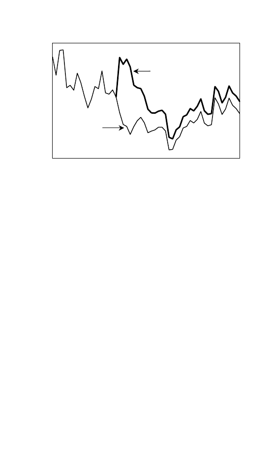
160
The Politics of Income Inequality in the United States
1.65
1.75
1.85
1.95
2.05
2.15
2.25
2.35
1947 1951 1955 1959 1963 1967 1971 1975 1979 1983 1987 1991 1995 1999
T20/B40 Ratio
Observed
Simulated
figure 6.4. Actual and Simulated Post-Government Inequality without LBJ
and 1965 Great Society Programs
I calculated the total impact that would eventually occur given a sus-
tained change in the explanatory variable. This simulation allows us
to see how long-term effects via error correction develop over time and
how an impermanent 4-year change in party control of the presidency
manifests itself over a 35-year period.
Figure 6.4 shows the observed path of post-government inequality
as well as its simulated path after replacing LBJ with a Republican
and eliminating the liberal policymaking of the Great Society with an
average year of lawmaking. The initial impact of the counter-factual
is impressive. The deviation between the simulated path of inequality
and its actual path peaks at 23 percent in 1969. However, due to the
dissipating effect of the temporary change in the presidency, the devi-
ation between the counter-factual and reality declines steadily from
1969 to 1981. Whereas simulated inequality is 23 percent higher than
observed inequality in 1969, this drops to a 4 percent discrepancy by
the 1980s and remains at a similar level to the end of the simulation.
By the end of the simulation, we are seeing only the effect of the policy
shift, which was a permanent reduction in policy liberalism that per-
sisted since 1965. While the gap between the two series is seemingly
small by the end, inequality would still have been 4 percent higher in
2000 had it not been for the Great Society.

Who Gets What and How
161
conclusion
The analysis in this chapter has clearly shown that politics matters
for distributional outcomes. When Democrats are in control of gov-
ernment and liberal policies are enacted, income inequality declines.
The mechanisms that generate this outcome are somewhat unexpected.
Redistribution is clearly the most explicit mechanism that government
uses to reduce inequality, but its impact is less responsive to macro
political change than is pre-redistribution inequality. This indicates
that political dynamics have a greater impact on distributional out-
comes via what I have called the market conditioning mechanism than
through explicit redistribution.
Furthermore, the analysis here shows that the dynamics of inequal-
ity reverberate back into the system, affecting the redistributive impact
of the state. Political change produces change in market inequality, and
changes in market inequality influence redistribution. Quite interest-
ingly, we have seen that when Democrats control the White House,
pre-redistribution inequality declines to such an extent that less redis-
tribution occurs. To the contrary, when a Republican takes over the
White House redistribution increases in tandem with overall levels of
post-government inequality.
Finally, we have seen direct evidence that public opinion shapes
income inequality. When public opinion shifts to the left, Democrats
are elected and policy moves in a liberal direction. These changes, in
turn, produce reductions in inequality. Public opinion is the engine that
drives the macro political system, and it is an engine that moves not
just politics, but also societal outcomes. The representational linkages
discovered in the macro politics model are not empty. Shifts in public
opinion are actually translated into outcomes that lie at the heart of
political contestation. These results suggest a variety of conclusions,
which I turn to in the final chapter.

7
Distribution, Redistribution, and the Future of
American Politics
The central goal of this book has been to explore the connection
between politics and distributional outcomes in America. I began with
a basic description of inequality in America and developed a theoreti-
cal framework for explaining distributional outcomes in which politics
plays a central role. I then discussed several ways in which the state
can influence distributional outcomes, categorizing these efforts into
explicit redistribution and market conditioning. The next step in the
argument was to discuss the nature of partisan and ideological dis-
agreement over distribution and redistribution in American politics. I
then moved to a series of analyses that examined how macro politi-
cal dynamics are connected to the dynamics of inequality in America.
In this concluding chapter, I synthesize the results, discuss the major
conclusions of my work, and explore predictions about the future of
American income inequality that grow out of my research.
how does politics influence who gets what?
The question of how politics influences who gets what has multiple
answers. Politics influences distributional outcomes in myriad ways,
even when we just focus on the macro level as I have done in this
book. In this section, I explore my major conclusions by providing
several answers to this question and discussing the importance of each
answer.
162

Distribution, Redistribution, the Future of American Politics 163
Politics Affects Both Distribution and Redistribution
One of the first messages that we should take is that focusing on only
redistribution or only inequality is insufficient if our goal is to under-
stand distributional outcomes. In this book I have examined both
distribution, the amount of economic inequality produced by the (gov-
ernment conditioned) market, and redistribution, how much inequality
is reduced when government takes from some and gives to others.
Breaking the distributional process into two stages accomplishes at
least two objectives. First, it provides us with an ability to examine
how “market” outcomes are influenced by political dynamics. Second,
it helps to avoid misleading conclusions that come from focusing just
on redistribution or money income inequality.
This second point deserves a bit more discussion. The standard
dependent variable in studies of American income inequality is either
family or household money income inequality. The problem with
money income is that it only partially accounts for the redistributive
impact of government. It includes benefits from cash transfer programs
but does not include in-kind benefits from programs such as food
stamps. Neither does it account for the impact of taxes. In other words,
money income is not a very useful concept because it is neither a clear
measure of market inequality nor a clear measure of post-government
inequality.
My strategy was to examine the distributional process in two explicit
stages, the first stage being primarily determined by market forces and
the second stage being influenced primarily by government policy. The
two stages combine to produce a final distribution of income, which
is a combination of market and governmental forces and can be mea-
sured utilizing the posttax post-transfer income concept. Creating the
measures necessary to follow this strategy is certainly much more time-
consuming than simply going to the latest Census publications and
recording the official level of income inequality that is defined by money
income. But following this strategy opened the door to an examina-
tion of government’s impact on both stages of the distributional process
and allowed an analysis of how market and political forces are inter-
connected. Many of the results discussed throughout the book would
simply be impossible without this two-stage conceptualization of the
distributional process in the United States.

164
The Politics of Income Inequality in the United States
The Power Resources of the Lower Classes Influence
Distributional Outcomes
If we want to know how politics influences who gets what in America,
the results here point toward power resources theory as a fruitful frame-
work. Despite the fact that power resources theory had its origins in the
expansive welfare states of Europe, the fundamental predictions apply
even in the liberal welfare state of the United States. The classic indica-
tors of both market and political power resources have their expected
impact on distributional outcomes. Decreasing levels of union mem-
bership, as an indicator of market power resources, have led to a less
equal distribution of income. In the United States, however, political
power resources take center stage as a predictor of distributional out-
comes. Left party strength produces substantial reductions in income
inequality in America.
1
This is all consistent with power resources the-
ory. In addition, to assess power resources theory in a new way that
goes beyond party control of government, I examined the ideological
tone of public policy. I find that leftward shifts in public policy reduce
economic inequities in the United States.
Who Gets What is Determined by, and is a Part of, the Macro
Political System
The macro politics literature has tended to examine the causes of
opinion change – media coverage, consumer confidence, thermostatic
feedback in response to policy – as well as the consequences of opinion
change – differential electoral outcomes and public policies. This book
moves the causal nexus forward by asking whether the macro political
dynamics that begin with the formation of public opinion and then
work themselves through representational linkage into policymaking
then also extend to policy outcomes – specifically the dynamics of
equality between the rich and the poor. The answer I have found is
a resounding yes.
That party control of government and the ideological tone of policy-
making influence distributional outcomes is an important contribution
and certainly extends the logic of the macro politics model to an
1
This is the case despite the commonly held view that there is little difference between
Democrats and Republicans in American politics. The Democrats may not be a tradi-
tional left party in the comparative sense, but differences between the American parties
are translated into divergent distributional outcomes when the electoral balance of
power shifts.

Distribution, Redistribution, the Future of American Politics 165
important societal outcome. However, that is not the end of the story.
What we have seen, by analyzing distributional outcomes in two stages,
is that just as policy affects the dynamics of inequality, the dynamics
of inequality reverberate back into the system, having causal effects
of their own. Yes, party control and policy influence market inequal-
ity, with shifts to the left decreasing inequality, but market inequality
also influences redistribution. When market inequality moves higher,
redistribution responds by shifting upward as well. By the same token,
redistribution is influenced by political dynamics but also conditions
market decisions thereby influencing the market distribution of income.
In this sense, gains and losses in economic equality are squarely within
the system of American political dynamics.
For Distributional Outcomes, Political Dynamics are Similar in
Importance to Demographic and Economic Change
Macro political dynamics, of course, are not the only factors that influ-
ence distributional outcomes. However, for far too long politics has
been relegated to the periphery. Economists in large part ignore the
role of government in producing distributional outcomes. Sociologists
have paid attention to politics, but political dynamics are still not cen-
tral to their story. Here we have seen that political change fits nicely
alongside both economic and demographic explanations of distribu-
tional outcomes. In fact, the evidence presented in this book points to
the conclusion that politics is nearly as important in explaining income
inequality as the more traditional economic and demographic expla-
nations. To minimize the importance of politics when assessing the
dynamics of inequality in the United States is pure folly. Politics is one
of the few avenues through which distributional outcomes can actually
be influenced. The aging of a population is a difficult thing to change.
So is the globalization of an economy. These factors influence inequal-
ity, and politics is one of the few ways that anything can be done. In
fact, as we have seen, politics not only directly influences distributional
outcomes, but can also indirectly influence inequality in ways such as
generating higher or lower levels of employment.
It’s the (Market) Economy, Stupid!
Typically, when people talk about the role of politics in distribu-
tional outcomes, the conversation is about explicit redistribution. The

166
The Politics of Income Inequality in the United States
debates in contemporary Washington that most often turn toward dis-
tributional concerns are those about tax cuts and benefit programs,
even ones like the marriage penalty tax that are not inherently linked
to redistributional questions. Democrats consistently criticize Repub-
licans for wanting to cut taxes for the rich, and Republicans accuse
Democrats of wanting to hand out money to the (undeserving) poor.
There is no doubt that taxes and transfers decrease inequality in Amer-
ica. When it comes to political dynamics, however, redistribution
is a relatively small part of the story. This is consistent with what
we observed when asking policymakers in Washington about their
distributional preferences.
According to the survey of House members reported in Chapter 3,
Democrats and Republicans largely agree that redistribution should
be avoided. This is why even Democrats are reticent to mention the
dreaded “R” word in debates about government programs. A favorite
critique of any expansion of an existing benefit program or new trans-
fer program, in fact, is that it is “just more redistribution.” Perhaps
because of this general agreement, the amount of redistribution that
occurs when left policies are enacted and Democrats control govern-
ment is only slightly different than when more conservative policies are
enacted by Republicans. The direct effect of a shift toward the left in
the macro polity is only a slight increase in redistribution.
The larger part of the story is market conditioning. As we saw in
Chapter 3, Democratic and Republican policymakers differ markedly
in their preferences regarding the use of the state to create conditions in
which economic opportunities are equalized. Democrats favor leftward
shifts in policy that condition the market in a way that benefits those
at the bottom, thus reducing market inequality. Policies supported by
Republicans, however, have exactly the opposite effect, moving mar-
ket inequality higher. When we look at the overall impact of political
change on post-government inequality, we see that politics has a much
greater impact via market conditioning than via explicit redistribu-
tion. It is important to note that this outcome may be unique to the
United States. In many countries, there is not such general disdain for
explicit redistribution, which brings redistribution more squarely into
the realm of political contestation and likely makes it more respon-
sive to macro political change and more important as a mechanism for
political impact on distributional outcomes.

Distribution, Redistribution, the Future of American Politics 167
Market Conditioning and Explicit Redistribution are Used in
Tandem to Influence Distributional Outcomes
While it is clear that market conditioning is the mechanism for equaliz-
ing distributional outcomes that is most responsive to macro political
dynamics, it is equally clear that policymakers do not face a choice
between either conditioning markets or explicitly redistributing income
in order to achieve distributional objectives. To the contrary, at
least when we focus on the direct effects of political dynamics on
redistribution and market inequality, we find that these mechanisms
are used in tandem. It would be incorrect to say that Democrats
favor redistribution and Republicans favor market mechanisms to
level the distributional playing field. The liberal policies favored by
Democrats both directly reduce market inequality and directly increase
redistribution. Democrats use both market mechanisms and explicit
redistribution to achieve their distributional goals. The same can be
said of Republicans, but the apparent distributional goals are differ-
ent. When Republicans enact conservative policies, the direct effect is
a reduction in redistribution and an increase in market inequality. It
simply is not the case that both parties have the same objectives but sim-
ply pursue different means to the same end. Both parties utilize market
conditioning and redistribution in pursuit of divergent distributional
outcomes.
Equalizing Distributional Outcomes Does Not Necessarily Lead to a
Bloated Traditional Welfare State
Republicans routinely charge that Democrats seek a welfare state that
is out of control, redistributing income in excessive amounts and thus
reducing the incentives necessary for innovation and economic growth.
They are partially correct, in that the increased redistribution that is
directly advocated by many Democrats does have the indirect conse-
quence of increasing pre-redistribution inequality. What unravels this
critique, however, is that the real action on distributive outcomes is
in the realm of market conditioning. The empirical evidence is clear.
When the direct and indirect effects of Democratic control of gov-
ernment are considered, they actually reduce redistribution, rather
than increase it. This is because Democrats reduce pre-redistribution
inequality by intervening in markets via market conditioning to such
an extent that redistributive programs become less necessary. At the

168
The Politics of Income Inequality in the United States
same time, Republicans indirectly increase redistribution by enacting
policies that exacerbate pre-redistribution inequality.
In the end, the distributional outcomes produced by the parties are
in line with expectations. Inequality rises when Republicans are in
charge and declines under Democratic control. However, it is interest-
ing to note that much of the equalizing impact induced by Democrats
can be attributed to market conditioning mechanisms rather than
explicit redistribution. These market conditioning mechanisms might
also be described as mechanisms that equalize economic opportuni-
ties. The caricature of Democrats as interested in equality of outcome
and Republicans as supportive of equality of opportunity seems only
partially correct. Democrats primarily achieve equality of outcome
through opening market opportunities to those at the bottom of the
pre-redistribution income scale. Republicans, it seems, oppose such
market conditioning schemes favored by Democrats and, in the pro-
cess, inadvertently induce the need for more government redistribution.
This is an ironic outcome to say the least.
Americans Can Modify Distributional Outcomes, If They Want To
Extending the macro politics model to distributional outcomes pro-
duced an additional important finding – public opinion influences dis-
tributional outcomes. Previous studies at the aggregate level have found
that public opinion influences policymaking, and this has been inter-
preted as successful democratic representation. But a well-functioning
democracy requires both representation and accountability. That is,
the policies enacted must actually make a difference. If public opinion
shifts toward the left, policy responds, but important societal out-
comes that should be influenced by changing government policy do
not respond, how successful would dynamic representation really be?
In addition, there has been recent debate about the responsiveness of
government to smaller segments of society. For example, members
of Congress may be more responsive to rich constituents than to the
poor (Bartels 2006, Bartels 2008) and Gilens (2006) argues that policy
responds to some segments of the population more than others, but
Soroka and Wlezien (2006) present evidence in favor of the idea that
macro policy is remarkably responsive to all segments of the popula-
tion. My analysis does not speak directly to the relative responsiveness
of policy and economic outcomes to different segments of the mass

Distribution, Redistribution, the Future of American Politics 169
public, but I can say that public opinion influences distributional
outcomes in the way we would expect. When public opinion shifts
toward the left, the composition of government and policies enacted
by government also shift toward the left. Then, these mass-driven
changes in government produce changes in the income distribution.
Pre-redistribution inequality is dramatically reduced, as is the over-
all level of inequality. If the mass public demands less inequality,
they can have it, and the reverse, of course, is also true. Regard-
less of one’s distributional preferences, this should be encouraging
news.
2
All of the conclusions discussed above point toward an overarch-
ing finding in support of my combination of the macro politics model
and power resources theory. While work in the macro politics tradi-
tion has focused on explaining the causes and consequences of public
opinion with a particular emphasis on how opinion is translated into
policy change, power resources theory pointed my examination of the
U.S. macro political system toward a focus on distributional outcomes.
Allowing these approaches, one from American politics and one from
comparative politics, to inform my work produced a useful framework
to study the distributional process in the United States.
By bringing these approaches together, I was not only able to
gain understanding of income inequality in America, but also able
to provide useful extensions both to the macro politics model and
power resources theory. I extended the macro politics model beyond
policymaking and found that distributional outcomes are of central
importance in U.S. macro political dynamics. Income inequality is not
only influenced by macro political change, but it is also apparent that
distributional outcomes shape the macro political system itself. With
regard to power resources theory, I found a great deal of support for
its predictions even in the least-likely case of the United States. I also
extended the logic of power resources theory to the realm of market
conditioning, finding that government-conditioned market inequality
2
Of course some historical legacies are very difficult to overcome with a mere change
in preferences. Black Americans, for example, have faced many institutional hurdles
to their economic advancement. My analysis only accounts for such historical legacies
in a very general empirical sense. Taking account of these historical processes would
require a much different analytical approach that the one employed here. Nonetheless,
the importance of history should not be dismissed.

170
The Politics of Income Inequality in the United States
is highly responsive to changes in the actualization of lower class power
resources.
The general point that can be drawn from this approach to under-
standing distributional outcomes in the United States is that commu-
nication and cross-fertilization between the fields of political science
can be very fruitful. In fact, such cross-field theoretical development
is probably most useful with regard to the largest and most impor-
tant unanswered questions in our discipline. While this may be readily
acknowledged by many of us in political science, we should actively
look for such cross-field opportunities.
american inequality in the twenty-first
century: looking forward
The last half of the twentieth century brought a great deal of change
in inequality. After decreasing for nearly 25 years, inequality began a
fairly steady march toward greater inequality during the early 1970s.
What is the future of inequality in America? There are several current
trends that shed some light on this question, and many political deci-
sions will in part determine the future path of inequality in the United
States.
There are a variety of trends which point to additional increases in
inequality in the future. Perhaps the most important of these trends is
our increasingly service-based, global economy. As service-sector jobs
that are often low-paying and free of union representation become
more prevalent, market inequality is likely to rise both because of
declining market power resources and the logic of industrialism. Like-
wise, an aging population with higher proportions of retirees and
elderly individuals with declining health puts upward pressure on mar-
ket inequality. Finally, the current trend toward ever higher executive
salaries (relative to other employees) is likely to feed an upward trend in
market income inequality. Market and demographic forces will almost
undoubtedly exacerbate economic inequality.
But as we have seen, market and demographic factors are only part
of the equation. Furthermore, market inequality is only the first stage
of the distributional process. While current trends certainly make it
seem likely that inequality will maintain its currently high level or even
increase further, the reaction of the state to these forces will in large part

Distribution, Redistribution, the Future of American Politics 171
determine the overall level of inequality present after market outcomes
are conditioned and government redistributes income. The path that
our society will choose is yet to be determined. The questions are how
we will deal with the market and demographic factors that tend to
force inequality higher and whether or not government will enact new
policies to reduce the gap between rich and poor.
Clearly, current economic and demographic trends are likely to
exert continued upward pressure on economic inequality in the United
States. If we focus on distributional outcomes as a part of the U.S. gov-
erning system, however, there is some reason to believe that income
inequality will not rise and may, in fact, fall in the near term. The
dynamics of the American macro political system begin with the for-
mation of public opinion, and we have seen that shifts in public opinion
eventually have distributional consequences. Current levels of Public
Mood liberalism suggest that equalizing changes are on the horizon.
The most recent macro public opinion data (Stimson’s Mood measure
in 2004) shows that public opinion is currently more liberal than it has
been since just before the Great Society programs were enacted in the
mid-1960s. The recent switch in party control of Congress shows that
these preferences are beginning to be translated into election outcomes
and will likely produce policy change in the near future.
If public opinion translates into greater Democratic strength in gov-
ernment and leftward shifts in public opinion, this will place downward
pressure on market income inequality. We must be careful to note
that this does not necessarily mean observed market inequality will
fall. To the contrary, if market and demographic change places suffi-
cient upward pressure on income inequality, liberal policies will simply
slow the growth of economic inequality. I suspect, however, that lib-
eral policy enactments will condition market outcomes sufficiently to
prevent market inequality from rising, and may even produce slight
reductions in inequality. The minimum wage will rise, protections
for foreign workers will be added to free trade agreements, executive
compensation will come under fire, and the elimination of workforce
discrimination will be vigorously pursued.
At the same time, Democrats will act to protect the largest redis-
tributive programs in the United States, most especially Social Security.
Privatization of Social Security, for example, will most likely not be a
serious part of the agenda if Democrats are powerful in Washington.

172
The Politics of Income Inequality in the United States
Proposals to expand the redistributive state will also be more likely to
gain traction. The most important changes on this front are likely to
come in the domain of health care. Democrats will likely try to either
create new redistributive programs to help millions of Americans pay
for health care, or they will create strong incentives or even require-
ments for employers to provide health benefits for their employees. The
former strategy for expanding health coverage would be an expansion
of the classic redistributive state, while proposals focused on employer
provision of benefits would be an example of market conditioning. In
the end, without major new redistributive programs, reduced market
inequality produced by liberal policy will decrease the need for redis-
tribution and will reduce overall levels of post-government inequality
while at the same time reducing explicit redistribution.
However, if Republicans once again gain ascendancy in Washing-
ton, tax cuts and reductions in domestic spending will likely be the
order of the day. Clearly, a current target of conservative policymak-
ers is Social Security. While it is clear that present benefit levels cannot
be maintained indefinitely, the most extreme ideas about privatizing
the program would lead to both a reduction in redistribution and an
increase in market inequality. The reasons for the reduction in redis-
tribution are obvious. Privatizing Social Security amounts to taking a
redistributive program and shifting it to the private sector. The increase
in market inequality is less certain, but without major controls on how
individuals might invest for their retirement, it is likely that some would
make very good choices and some would make rather bad ones. Those
who make good investment choices would leap far ahead of those mak-
ing worse decisions (or those who are just unlucky). This is not to say
that those at the bottom will not be better off in absolute terms (rather
than relative terms) under a private system. I do not have an answer
to that question. What seems clear, however, is that inequality would
increase under such a policy shift, and it would increase via both mech-
anisms of government influence on distributional outcomes that were
discussed in this book – market conditioning and redistribution.
The message of this book is that in the realm of distributional out-
comes, America in some part controls its own destiny. We are not
simply at the mercy of a global economy and demographic realities,
though those factors certainly do matter. Through politics, distri-
butional outcomes can be influenced dramatically. This influence is

Distribution, Redistribution, the Future of American Politics 173
not likely to occur via policies that explicitly redistribute income, but
instead can come through programs that augment the economic oppor-
tunities of the poor. The battle over distributional outcomes is an
essential part of the macro political system. If the American public
wants less inequality, they can affect this outcome by their preferences
and their voting behavior. By the same token, if Americans want to see
inequality increase as economic and demographic conditions continue
to place upward pressure on economic inequality, this outcome can
also be achieved. “Who gets what?” is in part determined by economic
and demographic factors that are difficult if not impossible to control,
but a large part of the answer to this question can be determined by
the dynamics of the macro political system – and citizens are a central
component in this system.


Appendix A: Congressional Questionnaire
«ID»
Thank-you for participating in this research project. Please answer each of the following questions
to the best of your ability.
1)
Please rank order the following outcomes from 1 to 7 with 1 being your most important priority
and 7 being the least important in your thinking when developing and voting on legislation.
_______ Increasing
Labor
Productivity
_______ Decreasing
Unemployment
_______ Increasing
Economic
Growth
_______
Decreasing Income Inequality
_______ Increasing
International
Trade
_______ Reducing
Poverty
_______ Controlling
Inflation
2)
The following is a list of occupations. On the line next to each occupation, please write about
how much (in US $) you think an average individual in each profession SHOULD earn during a
year, regardless of the amount they actually earn.
a) Computer
Programmer ..........................._____________________
b) Construction
Worker..............................._____________________
c) Janitor ....................................................._____________________
d)
CEO of Fortune 500 Company..............._____________________
e)
Fast Food Employee ..............................._____________________
f) Physician................................................._____________________
g) Plumber..................................................._____________________
h)
Factory Line Employee..........................._____________________
i) Human
Resources
Manager...................._____________________
j) Certified
Financial
Planner ....................._____________________
PLEASE COMPLETE REVERSE SIDE.
175

176
The Politics of Income Inequality in the United States
(3)
The items on this page refer to the following scale, where 1 indicates strong disagreement, 7
indicates strong agreement, and the numbers 2, 3, 4, 5, and 6 represent levels of agreement
between these two extremes.
Strongly Disagree
Strongly Agree
1
2
3
4
5
6
7
Circle the number that best approximates your opinion on each of the following statements:
(a) To ensure the best economic outcomes, government must sometimes intervene in the market.
1
2
3
4
5
6
7
(b) Society is better off when the income gap between the richest and poorest individuals is reduced.
1
2
3
4
5
6
7
(c) It is inappropriate for government to implement programs that redistribute income from the rich to
the poor.
1
2
3
4
5
6
7
(d) Government has a responsibility to modify some market processes in order to provide equal
economic opportunities to all citizens.
1
2
3
4
5
6
7
(e) Differences in income between the richest and poorest individuals in society are necessary to ensure a
strong economy.
1
2
3
4
5
6
7
(f) Government should provide explicit benefits to the following groups:
(i) Stockholders .............1
2
3
4
5
6
7
(ii) The
Aged ..................1
2
3
4
5
6
7
(iii) Small
Businesses.................1
2
3
4
5
6
7
(iv) The Poor ...................1
2
3
4
5
6
7
(v) Veterans ....................1
2
3
4
5
6
7
(vi) Corporate
Executives.................1
2
3
4
5
6
7
(vii) Children ....................1
2
3
4
5
6
7
(viii) Doctors......................1
2
3
4
5
6
7
Please include any additional comments you might have.

Appendix B: Measuring Income Inequality
over Time
The analysis focuses on three concepts related to the two stages of the
distributional process – pre-redistribution inequality, post-government
inequality, and explicit government redistribution. Measuring the con-
cepts is a relatively straightforward undertaking in the static context
of the year 2000. Data from the U.S. Census Bureau provides a wealth
of information about income at the household level. In the 2000
data, for example, we can learn with a reasonable degree of preci-
sion how much income each household received from a wide variety
of sources, such as wages, Social Security, dividends, Medicare bene-
fits, and unemployment. There are also reasonable estimates of taxes
that were paid within a household. Based on these data, the pre-
redistribution income of each household can be computed by excluding
income from all government sources. Post-government income can
be computed for each household by including income from govern-
ment sources and accounting for the amount of federal taxes paid.
With household level data on pre-redistribution income and post-
government income, a measure of inequality can be calculated for each
income concept, and the redistributional impact of government can be
calculated by finding the difference between pre-redistribution inequal-
ity and post-government inequality. Government redistribution could
then be reported in absolute or proportional terms.
This procedure works quite well going back in time to the late 1970s.
Prior to 1979, however, less detailed income data were collected. The
177

178
The Politics of Income Inequality in the United States
further one goes back in time, the less detailed the income data become.
An additional complication is the unit of analysis for which data are
available. In the cross-sectional data discussed in Chapters 1 and 2,
the unit of analysis was consistently the household – a group of related
or unrelated individuals living in the same dwelling. The household
as a unit of analysis is only available in the Census data since 1967.
Prior to that time, data were collected for families and for groups of
unrelated individuals. The household is the most appropriate unit of
analysis because households include both families living together and
unrelated individuals living together. So, the question is how to create
consistent measures of the three central concepts – pre-redistribution
inequality, post-government inequality, and explicit redistribution –
moving back to the late 1940s.
The standard practice in previous studies of American income
inequality has been to look only at inequality in family money income,
which remained available after the switch in 1967 to the household
as the standard unit of analysis in Census income data (Danziger and
Gottschalk 1995). With regard to the unit of analysis, the standard
practice is not ideal because examining families excludes unrelated indi-
viduals living together. With regard to income concept, money income
does not align well with either pre-redistribution or post-government
and certainly provides no options for examining the distributional
impact of government taxes and transfers. Thus, I will follow a
different strategy here.
The first issue is creating a series with a unit of analysis that is
consistent over time and includes the largest possible proportion of
the population. Ideally, there would be some way to examine house-
holds as the unit of analysis in the pre-1967 data. Unfortunately, this
cannot be done. Completely excluding unrelated individuals by focus-
ing only on families, however, is not a good option. Particularly as
the proportion of unrelated individuals living under the same roof
has increased over time, excluding such households from the analy-
sis provides a distorted picture of inequality over time – a picture that
includes a diminishing proportion of the total population. In order
to have measures of the three central concepts before 1967 but also
provide a consistent unit of analysis over time, I pursue an approach
of combining available information about the money income of fami-
lies and unrelated individuals. Combining information from these two

Appendix B: Measuring Income Inequality over Time
179
units of analysis produces lower estimates of inequality than measures
using the household as primary unit, but this strategy is certainly bet-
ter than examining families alone. Combining information on families
and unrelated individuals provides the opportunity to generate a long
series with a consistent unit of analysis that does not exclude unrelated
individuals.
The merging process works as follows. Since 1947, the Census
Bureau has collected the data necessary to compute inequality in money
income for unrelated individuals and families. While the individual-
level data that are necessary to compute Gini coefficients are not useful
for my purposes during the early years of income data collection,
aggregate income shares for each quintile for families and unrelated
individuals are regularly reported in Census Bureau publications. Using
this information produces an estimate of income inequality that is not
as accurate as that for households, but it provides a comparable mea-
sure during the full period of interest and allows a better estimate than
using only family income.
In 1967, for example, the first quintile of families had about 5.5 per-
cent ($26.8 billion) of aggregate family money income ($487.7 billion).
The first quintile of unrelated individuals had 3 percent ($1.40 billion)
of aggregate money income ($46.6 billion). When these two groups
are combined, the first quintile held $28.2 billion of $534.3 billion,
for an income share of 5 percent. Table b.1 shows similar data for all
five income quintiles in 1967. As the table indicates, combining families
and individuals does not reproduce the household data perfectly in that
it consistently provides a lower estimate of inequality. However, this
combination approach provides comparable money income share data
going back to 1947 that is far superior to using family income alone.
table b.1. Distribution of Money Income for Families, Unrelated
Individuals, and Households: 1967
Quintile
(%)
Families
(%)
Unrelated Individuals
(%)
Combined
(%)
Households
(%)
1
6
3
5
4
2
12
8
12
11
3
18
13
17
17
4
24
24
23
24
5
40
52
41
44

180
The Politics of Income Inequality in the United States
The second problem is creating measures of pre-redistribution
inequality and post-government inequality with less and less detailed
information about income sources as one moves back in time. In order
to generate measures of the three central distributional outcomes of
interest for my analysis, I follow a strategy that is similar to that of
Smeeding (1979) and Browning and Johnson (1979). The logic of
this method is illustrated in Table b.2. The money income received
by each income quintile is the starting point of this method, and this
distribution is reported in the first row of the table based on data
from 2000. Money income, however, includes income from govern-
ment cash transfers, so these must be removed before inequality in
pre-redistribution income can be derived. While extremely detailed
data about the distribution of cash transfer benefits is not available
consistently in income data back to 1947, budgetary data that report
the expenditures of federal government programs that distribute cash
benefits are available.
In years that detailed income data are available (particularly
after 1979), it is a straightforward matter to allocate federal cash
table b.2. A Method for Computing Income Distribution Over
Time Illustrated with Data from
2000
Money Income Quintile ($Billions)
Income Component
1
2
3
4
5
Total
1. Money Income
$267
$578
$925
$1395
$2903
$6077
Subtract:
2. Cash Transfers
$270
$141
$76
$53
$47
$587
Add:
3. Underreporting
$49
$65
$86
$111
$236
$547
Equals:
4. Pre-Redist.
$
46
$
502
$
935
$
1453
$
3092
$
6037
Share
1%
8%
16%
24%
51%
Add:
5. Cash Transfers
$270
$141
$76
$53
$47
$587
6. In-kind Benefits
$209
$85
$53
$41
$43
$431
Subtract:
7. Taxes
$17
$83
$215
$381
$961
$1657
Equals:
8. Post-Gov’t.
$
508
$
645
$
849
$
1166
$
2221
$
5398
Share
10%
12%
16%
22%
41%

Appendix B: Measuring Income Inequality over Time
181
transfer outlays across the five income quintiles. Based on the detailed
individual-level data, we know the proportion of total cash transfers
received by each income quintile. This information combined with bud-
get data on cash transfers in a given year can be used to determine the
amount of income received by each quintile. While it may seem odd to
go through this convoluted process for years in which income source
specific unit-level data are available, maintaining consistency in mea-
surement in the more recent data necessitates applying similar methods
to data over the entire period of analysis.
For earlier years when detailed income data are not available, a
similar logic applies, but we have less information available regarding
which income quintiles received transfers. Fortunately, fiscal incidence
studies have paid a great deal of attention to the distribution of gov-
ernment benefits across the income quintiles (Browning 1985). What
we have learned from fiscal incidence studies is that the distribution
of federal cash transfers across income quintiles has remained rel-
atively steady over time. Thus, we can use what is known about
the distribution of cash transfers in later years with highly detailed
unit-level data to allocate cash transfers across the income quintiles
in earlier years when the data are less detailed.
1
This adjustment is
shown in the second row of Table b.2. One further adjustment based
on known under-reporting of certain forms of income in the Census
data is shown in the third row. Adjusting for under-reporting pro-
duces pre-redistribution quintile shares which are reported in the fourth
row. The pre-redistribution quintile shares computed in this way are
almost identical to those reported in Chapter 3, with the only discrep-
ancy being slightly less inequality than in the household data reported
earlier, which is to be expected.
The fifth, sixth, and seventh rows of the table present adjustments to
pre-redistribution income that are necessary to create post-government
income – cash transfers are reintroduced, the effects of in-kind benefits
are added, and taxes are subtracted. As with cash transfers, consistently
available budgetary data are used to determine the total government
expenditures for in-kind benefits such as food stamps and Medicare.
1
The proportional allocation of cash transfers among the income quintiles in years prior
to 1979 are computed based on the formula computed with the detailed unit-level data
available in 1979.

182
The Politics of Income Inequality in the United States
Since the distribution of these benefits is essentially identical for years in
which unit-level in-kind benefit income data are available, these expen-
ditures are distributed among the five income quintiles using the same
formula each year, with the lowest quintiles receiving most of these
expenditures. For taxes, the Internal Revenue Service has reported
the total amount of revenue collected via personal tax vehicles for
many years. The distribution of these taxes for each year is based on
tax incidence research (Pechman and Okner 1974, Pechman 1985).
Despite massive changes in tax laws, for most years the top quintile
paid between 55 percent and 65 percent of these taxes and the lowest
quintile paid no more than 3 percent.
The amount of post-government income received by each income
quintile and the share of aggregate income this amount represents are
displayed at the bottom of Table b.2. Using the methods described
above, the 2000 data reported in this table are extremely close to
the estimates produced by the more detailed individual-level analy-
sis discussed in Chapter 3, again with the expected difference that
household data used in Chapter 3 produce slightly higher estimates
of post-government inequality than the estimate here. Most impor-
tantly, however, applying this method allows for a valid estimate of
pre-redistribution inequality, post-government inequality, and explicit
redistribution in every year from 1947 to 2000. The Gini coefficient
cannot be computed accurately using anything less than decile income
shares (I have only quintile shares), but calculating the T20/B40 ratio
(ratio of the aggregate income of the top 20 percent of the income
distribution to the bottom 40 percent) is possible. Using the proce-
dures discussed above, we see that the pre-redistribution T20/B40 ratio
was 5.64 and the post-government ratio was 1.93 in the year 2000 –
an absolute reduction of 3.71 and a proportional reduction of 66
percent.
It is important to point out that the proportional reduction in
inequality is higher in my data than in the LIS data utilized in
cross-national research due to the fact that cross-national studies rely
primarily on the Gini coefficient. The Gini coefficient is less sensitive to
changes in distribution at the extremes of the income distribution than
the T20/B40 ratio. The T20/B40 ratio, in fact, focuses exclusively on
changes in distribution between the top and the bottom. So, if inequal-
ity in the middle of the income distribution (inequality among those in

Appendix B: Measuring Income Inequality over Time
183
the middle two or three quintiles) remains fairly constant and redistri-
bution occurs primarily between the top and bottom of the distribution,
the T20/B40 ratio will be much more sensitive to such redistribution
than the Gini. Given the liberal welfare state regime present in the
United States, which emphasizes means-tested and targeted welfare
state programs, it is fully expected that my measure of inequality would
produce higher estimates of redistribution than a measure of redistri-
bution based on changes in the Gini coefficient. Movement over time
in the two types of measures, however, would be similar.


Bibliography
Alesina, Alberto and Edward Glaeser. 2006. Fighting Poverty in the US and
Europe: A World of Difference. New York: Oxford University Press.
Alesina, Alberto and Howard Rosenthal. 1995. Partisan Politics, Divided
Government, and the Economy. New York: Cambridge University Press.
Banerjee, Anindya. 1986. “Exploring Equilibrium Relationships in Econo-
metrics through Static Models: Some Monte Carlo Evidence.” Oxford
Bulletin of Economics and Statistics 48(3): 253–277.
Banerjee, Anindya, Juan Dolabo, John Galbraith and David F. Hendry. 1993.
Co-integration, Error Correction, and the Econometric Analysis of Non-
Stationary Data. New York: Oxford University Press.
Bartels, Larry M. 2006. “Is the Water Rising? Reflections on Inequality and
American Democracy.” PS: Political Science and Politics 39(1): 39–42.
Bartels, Larry M. 2008. Unequal Democracy: The Political Economy of a New
Guilded Age. Princeton: Princeton University Press.
Beach, Charles M. and Frederick S. Balfour. 1983. “Estimated Payroll Tax
Incidence and Aggregate Demand for Labour in the United Kingdom.”
Economica 50(197): 35–48.
Bradley, David, Evelyne Huber, Stephanie Moller, François Nielsen and
John Stephens. 2003. “Distribution and Redistribution in Post-Industrial
Democracies.” World Politics 55(2): 193–228.
Brandolini, Andrea and Timothy Smeeding. 2006. “Patterns of Economic
Inequality in Western Democracies: Some Facts on Levels and Trends.”
PS: Political Science and Politics 39(1): 21–26.
Browning, Edgar K. 1985. “Tax Incidence, Indirect Taxes, and Transfers.”
National Tax Journal 38(4): 525–533.
Browning, Edgar K. 2002. “The Case Against Income Redistribution.” Public
Finance Review 30(6): 509–530.
185

186
Bibliography
Browning, Edgar K. and William R. Johnson. 1979. The Distribution of the
Tax Burden. Washington: American Enterprise Institute for Public Policy
Research.
Campbell, Angus, Philip E. Converse, Warren E. Miller and Donald E. Stokes.
1960. The American Voter. New York: Wiley.
Dahl, Robert A. 1967. Pluralist Democracy in the United States. Chicago:
Rand McNally.
Danziger, Sheldon and Peter Gottschalk. 1995. America Unequal. New York:
Russell Sage Foundation.
Danziger, Sheldon, Robert Haveman and Robert Plotnick. 1981. “How
Income Transfers Affect Work, Savings, and the Income Distribution.”
Journal of Economic Literature 19(3): 975–1028.
Davidson, James E. H., David F. Hendry, F. Srba and S. Yeo. 1978. “Econo-
metric Modelling of the Aggregate Time-Series Relationship between
Consumers’ Expenditure and Income in the United Kingdom.” Economic
Journal 88(352): 661–692.
De Boef, Suzanna. 2001. “Modeling Equilibrium Relationships: Error Correc-
tion Models with Strongly Autoregressive Data.” Political Analysis 9(1):
78–94.
De Boef, Suzanna and Jim Granato. 1999. “Testing for Cointegrating Rela-
tionships with Near-Integrated Data.” Political Analysis 8(1): 99–117.
De Boef, Suzanna and Luke Keele. 2008. “Taking Time Seriously.” American
Journal of Political Science 52(1): 184–200.
Engle, Robert F. and Clive W. J. Granger. 1987. “Co-integration and Error
Correction: Representation, Estimation, and Testing.” Econometrica
55(2): 251–276.
Enns, Peter K. and Paul M. Kellstedt. 2008. “Policy Mood and Political Sophis-
tication: Why Everybody Moves Mood.” British Journal of Political
Science 38: 433–454.
Erikson, Robert S., Michael. MacKuen and James A. Stimson. 2002. The
Macro Polity. New York: Cambridge University Press.
Esenwein, Gregg A. 2001. The Federal Income Tax and the Treatment of
Married Couples: Background and Analysis. Technical Report RL30800
Congressional Research Service.
Esping-Andersen, Gøsta. 1990. The Three Worlds of Welfare Capitalism.
Princeton, N.J.: Princeton University Press.
Euromonitor. 2002. International Marketing Data and Statistics 2002, 26th
ed. Chicago: Euromonitor International.
Gilens, Martin. 2006. “Inequality and Democratic Responsiveness.” Paper
presented at the annual meeting of the American Political Science Associ-
ation, Philadelphia, PA, Aug. 31–Sept. 3.
Gottschalk, Peter and Timothy M. Smeeding. 1997. “Cross National Compar-
isons of Earnings and Income Inequality.” Journal of Economic Literature
35(2): 633–687.

Bibliography
187
Harris, Fredrick C., Valeria Sinclair-Chapman and Brian D. McKenzie. 2004.
Countervailing Forces in African-American Civic Activism, 1973–1994.
New York: Cambridge University Press.
Heclo, Hugh. 1974. Modern Social Politics in Britain and Sweden. New
Haven, CT: Yale University Press.
Hibbs, Douglas. 1987. The American Political Economy: Macroeconomics
and Electoral Politics. New York: Cambridge University Press.
Hibbs, Douglas A., Jr. and Christopher Dennis. 1988. “Income Distribution
in the United States.” American Political Science Review 2(2): 467–489.
Hicks, Alexander and Duane H. Swank. 1984. “Governmental Redistri-
bution in Rich Capitalist Democracies.” Policy Studies Journal 13(2):
265–287.
Hicks, Alexander and Duane H. Swank. 1992. “Politics, Institutions, and
Welfare Spending in Industrialized Democracies, 1960–1982.” American
Political Science Review 86(3): 658–674.
Hicks, Alexander and Joya Misra. 1993. “Political Resources and the Growth
of Welfare in Affluent Capitalist Democracies, 1960–1982.” American
Journal of Sociology 99(3): 668–710.
Hicks, Alexander M. 1999. Social Democracy and Welfare Capitalism: A Cen-
tury of Income Security Politics. Social democracy and welfare capitalism
Ithaca, N.Y.: Cornell University Press.
Holmlund, Bertil. 1983. “Payroll Taxes and Wage Inflation: The Swedish
Experience.” Scandinavian Journal of Economics 85(1): 1–15.
Howard, Christopher. 1999. The Hidden Welfare State: Tax Expenditures
and Social Policy in the United States. Princeton, NJ: Princeton University
Press.
Huber, Evelyne, Charles Ragin and John D. Stephens. 1993. “Social Democ-
racy, Christian Democracy, Constitutional Structure and the Welfare
State.” American Journal of Sociology 99(3): 711–749.
Huber, Evelyne and John D. Stephens. 2001. Development and Crisis of
the Welfare State: Parties and Policies in Global Markets. Chicago: The
University of Chicago Press.
Iversen, Torben. 2005. Capitalism, Democracy, and Welfare. New York:
Cambridge University Press.
Jacobs, Lawrence and Jheda Skocpal. 2005. Inequality and American Democ-
racy: What we Know and What we Need to Learn. New York: Russell
Sage Foundation.
Johnston, David Cay. 2007. Free Lunch: How the Wealthiest Americans
Enrich Themselves at Government Expense (and Stick You with the Bill).
New York: Portfolio.
Keister, Lisa A. 2000. Weath in America: Trends in Wealth Inequality. New
York: Cambridge University Press.
Kellstedt, Paul, Gregory E. McAvoy and James A. Stimson. 1996. “Dynamic
Analysis with Latent Constructs.” Political Analysis 5(1): 113–150.

188
Bibliography
Kelly, Nathan J. 2004. “Does Politics Really Matter? Policy and Government’s
Equalizing Influence in the United States.” American Politics Research
32(3): 264–284.
Kelly, Nathan J. 2005. “Political Choice, Public Policy, and Distributional
Outcomes.” American Journal of Political Science 49(4): 865–880.
Korpi, Walter. 1978. The Working Class in Welfare Capitalism: Work,
Unions, and Politics in Sweden. London: Routledge and Kegan Paul.
Korpi, Walter. 1983. The Democratic Class Struggle. London: Routledge and
Kegan Paul.
Korpi, Walter. 1985. “Power Resources Approach vs. Action and Conflict: On
Causal and Intentional Explanations in the Study of Power.” Sociological
Theory 3(2): 31–45.
Korpi, Walter. 1989. “Power, Politics, and State Autonomy in the Devel-
opment of Social Citizenship: Social Rights during Sickness in Eighteen
OECD Countries since 1930.” American Sociological Review 54(3):
309–329.
Lipset, Seymour Martin and Gary Marks. 2000. It Didn’t Happen Here: Why
Socialism Failed in the United States. New York: Norton.
Lockhart, Charles. 1991. “American Exceptionalism and Social Security:
Complementary Cultural and Structural Contributions to Social Program
Development.” Review of Politics 53(3): 510–529.
Mayhew, David R. 2005. Divided We Govern: Party Control, Lawmaking and
Investigations, 1946–2002. 2nd ed. New Haven: Yale University Press.
McCarty, Nolan, Keith Poole and Howard Rosenthal. 2006. Polarized Amer-
ica: The Dance of Ideology and Unequal Riches. Cambridge: MIT
Press.
McGuire, Kevin T. and James A. Stimson. 2004. “The Least Dangerous Branch
Revisited: New Evidence on Supreme Court Responsiveness to Public
Preferences.” Journal of Politics 66(4): 1018–1035.
Meltzer, Alan H. and Scott F. Richard. 1981. “A Rational Theory of the Size
of Government.” Journal of Political Economy 89(4): 914–927.
Moffitt, Robert. 1992. “Incentive Effects of the U.S. Welfare System: A
Review.” Journal of Economic Literature 30(1): 1–61.
Myles, John. 1984. Old Age and the Welfare State: The Political Economy of
Public Pensions. Boston: Little, Brown.
Orloff, Ann Shola. 1996. “Gender and the Social Rights of Citizenship: The
Comparative Analysis of Gender Relations and Welfare States.” American
Sociological Review 58(3): 303–328.
Page, Benjamin I. and James Roy Simmons. 2000. What Government Can
Do: Dealing with Poverty and Inequality. Chicago: University of Chicago
Press.
Page, Benjamin I. and Robert Y. Shapiro. 1992. The Rational Public: Fifty
Years of Trends in Americans’ Policy Preferences. Chicago: University of
Chicago Press.

Bibliography
189
Pampel, Fred C. and John B. Williamson. 1988. “Welfare Spending in
Advanced Industrial Democracies, 1950–1980.” American Journal of
Sociology 50(6): 1424–1456.
Pechman, Joseph A. 1985. Who Paid the Taxes, 1966–85? Washington, D.C.:
Brookings Institution.
Pechman, Joseph A. and Benjamin A. Okner. 1974. Who Bears the Tax
Burden? Washington: Brookings Institution.
Peppard, Donald M., Jr. and Douglas B. Roberts. 1977. Net Fiscal Incidence
in Michigan: Who Pays and Who Benefits? Lansing, MI: Michigan State
University.
Plotnick, Robert D., Eugene Smolensky, Eirick Evenhouse and Siobhan Reilly.
2000. The Twentieth-Century Record of Inequality and Poverty in the
United States. In The Cambridge Economic History of the United States,
ed. Stanley L. Engerman and Robert E. Gallman. Vol. 3, New York:
Cambridge University Press.
Pontusson, Jonas and Lane Kenworthy. 2005. “Rising Inequality and the Poli-
tics of Redistribution in Affluent Countries.” Perspectives on Politics 3(3):
449–471.
Quadagno, Jill. 1988. The Transformation of Old Age Security: Class and
Politics in the American Welfare State. Chicago: University of Chicago
Press.
Sawyer, Malcom. 1976. Income Distribution and Poverty in OECD Countries.
Technical Report 0474-5574 Organisation for Economic Co-operation
and Development.
Skocpol, Theda. 1979. States and Social Revolutions: A Comparative Anal-
ysis of France, Russia, and China. New York: Cambridge University
Press.
Skocpol, Theda. 1992. Protecting Soldiers and Mothers: The Political Origins
of Social Policy in the United States. Cambridge, MA: Harvard University
Press.
Skocpol, Theda and Edwin Amenta. 1986. “States and Social Policies.” Annual
Review of Sociology 12: 131–157.
Smeeding, Timothy M. 1979. “On the Distribution of Net Income: Comment.”
Southern Economic Journal 45(3): 932–944.
Soroka, Stewart N. and Christopher Wlezien. 2006. “Heterogeneity and
Homogeneity in Opinion-Policy Dynamics.” Paper presented at the
annual meeting of The American Political Science Association, Philadel-
phia, PA, Aug. 31–Sept. 3.
Stenberg, Carl W. and David B. Walker. 1977. “The Block Grant: Lessons
from Two Early Experiments.” Publius 7(2): 31–60.
Stephens, John D. 1979. The Transition from Capitalism to Socialism. London:
Macmillan.
Stimson, James A. 1999. Public Opinion in America: Moods, Cycles, and
Swings. 2nd ed. Boulder, CO: Westview Press.

190
Bibliography
Stimson, James A., Michael B. MacKuen and Robert S. Erikson. 1995.
“Dynamic Representation.” American Political Science Review 89(3):
543–565.
Stonecash, Jeffrey M., Mark D. Brewer and Mack D. Mariani. 2002. Diverging
Parties: Social Change, Realignment, and Party Polarization. Boulder:
Westview Press.
Swank, Duane. 2002. Global Capital, Political Institutions, and Policy Change
in Developed Welfare States. New York: Cambridge University Press.
Truman, David. 1951. The Governmental Process. New York: Alfred A.
Knopf.
Van Arnhem, J. Corina M. and Guert J. Schotsman. 1982. Do Parties Affect the
Distribution of Incomes? The Case of Advanced Capitalist Democracies.
In The Impact of Parties, ed. Francis G. Castles. Beverly Hills, CA: Sage
Publications.
Verba, Sidney and Gary R. Orren. 1985. Equality in America: The View From
the Top. Cambridge, MA: Harvard University Press.
Vroman, Wayne. 1974. “Employer Payroll Taxes and Money Wage
Behaviour.” Applied Economics 6(3): 189–204.
Wallerstein, Michael. 1999. “Wage-Setting Institutions and Pay Inequality
in Advanced Industrial Societies.” American Journal of Political Science
43(3): 649–680.
Weissburg, Robert. 2006. “Politicized Pseudo Science.” PS: Political Science
and Politics 39(1): 33–42.
Weitenberg, Johannes. 1969. “The Incidence of Social Security Taxes.” Public
Finance 24(2): 193–208.
Wilensky, Harold. 1975. The Welfare State and Equality. Berkeley: University
of California Press.
Wlezien, Christopher. 1995. “The Public as Thermostat: Dynamics of Pref-
erences for Spending.” American Journal of Political Science 39(4):
981–1000.

Index
absolute vs. relative economic
conditions, 149
aged population
demographic trends, 170
explanation of redistribution, 138
group-based politics, 77, 78
health care, 25, 33, 45
as influence on pre-redistribution
inequality, 115, 154
as influence on redistribution, 108,
109, 131, 132, 151, 152
position in income distribution, 37
tax system and, 57
Annual Demographic Survey, see
Current Population Study
Annual Social and Economic
Supplement, see Current
Population Study
Bush, George H.W., 97, 99, 100
Bush, George W., 44, 58
Bush, Neil, 44
Carter, Jimmy, 99, 100
cash benefits, 26
distributional effects of, 24
as income source, 94
income distribution and, 7
as income source, 4, 5
in measures of inequality, 163,
179, 180
causal ordering, 142
Census Bureau, United States
consumer expenditure data, 4
income data, 4–6, 9, 35
measuring inequality, 94, 163,
176–180
charity, 18
Christian Democratic Party, 87
Clinton, Bill, 58, 65, 97, 99, 100
Congress, U.S., 80, 168, 171
House of Representatives, 67–78
attitudes toward distributional
outcomes, 67, 74, 166
attitudes toward redistribution
and economic opportunity,
76
marriage tax penalty and,
58–63, 65, 66
in models of inequality, 114
in models of redistribution, 102,
108, 109
preferred levels of inequality, 72
preferred salary by
occupation, 70
priority of distributional
outcomes, 72
191

192
Index
Congress, U.S., (cont.)
support for group-based
benefits, 77
survey data, 67–69
influence on inequality, 109, 114
influence on redistribution, 108,
109, 111
marriage tax penalty and, 58
policy trends, 130
Senate, 102, 108, 109, 114
marriage tax penalty and,
58–60, 62, 63, 65, 66
tax policy and, 54, 56
counter-factual, 158–160
Current Population Study, 4, 5,
25, 33
deindustrialization, 102, 108–109,
114–115
Democratic Party, 164, 166–168,
171, 172
control of government
as influence on redistribution,
106, 155
as influence on unemployment,
137, 139
control of presidency, 102, 131
as influence on
pre-redistribution inequality,
99, 114–116, 143–144,
152, 154
as influence on redistribution,
100, 108–110, 152, 155
as influence on unemployment,
143, 149
influence on income inequality,
115, 140, 157
simulated effect on
inequality, 159
distributional outcomes and, 81
distributional preferences of, 67,
70–72
divided government and, 111
House survey, 68, 69
lower class interests and, 128
macro politics model and, 123,
125, 141, 146–150
marriage tax penalty and, 61, 66
opposition to Republican
proposals, 61, 62, 66
proposals, 59, 60, 62–63, 66–67
roll call voting, 61, 65
policy priorities, 70, 72, 73
preferred role of government,
74–76
relative ideological position, 92
strength in Congress, 108, 109,
114
strength in House, 102
strength in Senate, 102
support for group-based benefits,
70, 76–78
taxation and, 27, 38
welfare spending and, 92
demographics
data, 4
as influence on pre-redistribution
inequality, 115
influence on income inequality,
138, 142, 150, 165, 172, 173
future trends, 170, 171, 173
logic of industrialism and, 15,
86, 108
direct effects, 141, 151, 152
defined, 143
of Medicare, 45
of party control, 116, 125, 144
of policy, 144, 149
of political variables, 137, 139,
147, 152, 166, 167
of taxes, 28
disability benefits, 5, 35, 40, 95
distributional consequences
of benefit programs, 31, 36
group-based benefits and, 70
ideological differences and, 72
macro politics model and, 14
of market conditioning, 42–45,
47, 48
marriage tax penalty and, 66
measurement, 25, 27

Index
193
of public opinion, 171
of public policy, 13, 122, 134
tax policy and, 24, 36
distributional process, stages of
measurement, 94, 176
posttax, post-transfer inequality,
88
power resources theory, 85, 87,
88, 93
theoretical importance of, 18,
163, 165
divided government, 103, 109,
111, 116
Earned Income Credit, see taxes,
Earned Income Credit
economic conditions, United States,
2–3
consumer expenditures, 3, 4
median home price, 3
median income, 3
economic growth, 72, 73, 167
economic opportunity, 43, 76, 92
education
distributional consequences of, 13
higher education benefits, 37
logic of industrialism thesis
and, 102
market conditioning and, 42–45
as power resource, 82
tax deductions, 28
educational assistance, 5, 35, 45, 95
Eisenhower, Dwight D., 99, 100
elderly population, see aged
population
elections, 119, 121
future of inequality and, 172
future policy change and, 171
macro politics model and, 13,
123, 146
marriage tax penalty and, 58
as mechanism of
accountability, 80
as mechanism of responsiveness,
80, 121, 123
in model of income inequality, 16
political engagement and, 119
endogenous variables, 124, 125,
139, 144–146
entitlements, 31, 40
error correction models, 130,
144, 159
general description, 103–106
pre-redistribution inequality, 111
redistribution, 106, 109, 131, 132
exogenous variables, 145, 146
female labor force participation, 12,
102, 114
food stamps, 24, 31, 35, 95,
163, 180
Ford, Gerald, 2, 99, 100
GDP, see Gross Domestic Product
Gini coefficient
comparative data, 8
compared to other measures, 10,
94, 97, 181, 182
data requirements, 94, 178, 181
definition, 8
impact of government programs
on, 30, 33, 34, 36
trends in United States, 9, 10
globalization, 165, 172
Great Depression, 2, 9, 51
Great Society, 130, 156, 158,
160, 171
Gross Domestic Product, 2, 3, 149
health care, 38
benefits as income source, 26
Medicaid, 36
Medicare, 33, 45
as political issue, 40, 172
tax deductions, 18
housing subsidies, 35

194
Index
ideology
of Christian parties, 88
common space scores, 109
of U.S. Congress, 67, 70, 74, 76
conservative sentiment, 40
House survey and, 68, 69
macro politics model and, 14,
121, 122
position of U.S. parties, 92
public opinion and, 121
public policy
current debate, 172
as indicator of power
resources, 127
as influence on distributional
outcomes, 19, 125, 130, 132,
133, 164
measurement, 128, 129
taxation and, 27
in theory of income inequality, 80
immigration
as influence on pre-redistribution
inequality, 115–116, 133, 144,
152, 159
as influence on redistribution, 108
logic of industrialism and, 108
redistributive policy and, 108
in-kind benefits
distributional effects of, 24
income measurement and, 26, 94,
163, 180, 181
Medicare, 33
income concepts
money income, see money income
post-government, see
post-government income
posttax post-transfer, see
post-government income
pre-redistribution, see
pre-redistribution income
pretax pre-transfer, see
pre-redistribution income
income inequality
contemporary United States, 4–9
in comparative perspective, 7–9
government impact on, 36–48
occupations and, 6, 7
pre-redistribution, 26, 33
quintile income shares, 5, 6, 26,
27, 29
education and, 43, 44
empirical analysis
methodological techniques and,
137, 139, 142, 143
results of, 154, 164
empirical analysis of, 109, 111,
114–116
methodological techniques
and, 103
influence of party control on, 81,
99, 168
influence of political dynamics on,
156, 162
compared to economic
variables, 20, 165
direct effect of, 138
effect via economic variables
and, 165
indirect effect of, 149
macro politics model and, 80
via market conditioning and
redistribution compared, 152,
155
as mechanism of societal
influence, 165, 172
power resources theory and, 81
simulation of, 158
total effect of, 138, 139, 147
via market conditioning and
redistribution compared, 166
influence of public opinion on
indirect effect of, 138, 141,
142, 149
as mechanism of popular
control, 168
total effect of, 158, 169
influence of public policy on
macro policy and, 126–128
macro politics model and, 123
marginal changes and, 126
mechanisms of impact and, 23,
125, 134

Index
195
micro policy and, 126, 127
permanence of effect of, 134
power resources theory and,
124, 125
question introduced, 23
theoretical implications of, 164
macro politics model and, 13, 14,
80, 138, 141, 168, 169, 173
market conditioning and, 19, 41,
42, 158
marriage tax penalty and, 58
measurement of, 88, 89, 179
mechanisms of government impact
on, 20, 163, 165, 167
political disagreement over
distributional preferences
and, 74
government action and, 67,
74, 76
power resources theory and
mechanisms of impact and, 15
previous tests of, 87, 88, 90
role of class, 123
theoretical foundations, 81, 82,
85, 86, 89, 125
theoretical model, 15
simulation of post-government
inequality, 159
size of welfare state and, 167
social welfare programs and, 12
theoretical model of, 101
economic theories and, 141
implications of, 101, 170
introduced, 12, 16, 17
macro politics model and,
127, 169
policy liberalism in, 130
power resources and, 89, 90, 98
power resources theory and,
169
total effect of explanatory
variables on, 151
total effect of politics on, 156
trends in United States, 9–12
future, 170–172
Gini, 9, 10
income share, top 5 percent,
10, 11
pre-redistribution, 95, 97
two stages of distributional
process, 165
unemployment and, 142
welfare state theory and, 14, 15
income tax, see taxes, income
indirect effects
calculation of, 144, 145
causal ordering and, 143
defined, 137, 143
of feedback loop, 154
of higher order effects of policy, 29
of party control of presidency,
152, 155, 167
of political factors on
redistribution, 140
of politics on inequality, 137,
142, 155
of politics on pre-redistribution
inequality, 152
of public opinion, 158
inflation, 3, 72, 73
job training, 19, 127
Johnson, Lyndon B.
Great Society and, 130
Medicare and, 31
pre-redistribution inequality
and, 99
redistribution and, 100
simulated distributional impact of
presidency, 156, 158–160
judicial branch, 121
Kennedy, John F., 99, 100
Kennedy, Senator Ted, 63
labor market
as intervening variable, 150
logic of industrialism thesis
and, 108
market conditioning and the,
41–43, 45

196
Index
labor market (cont.)
in models of inequality, 138
power resources theory and, 90
reduction in work effort, 140
variables related to, 114, 115
labor unions
collective bargaining and, 83
direct and indirect effects on
income inequality, 142
as economic power resource, 15,
16, 18, 82, 83
influence on election
outcomes, 125
in model of pre-redistribution
inequality, 115, 133, 134, 138,
144, 151, 152, 154
power resources theory and, 15,
85, 88, 125
laws (see also legislation)
gay marriage, 54
as measure of public policy, 126,
128, 129, 134
property, 56
in simulation of distributional
outcomes, 159
tax, 181
legislation (see also laws)
education policy, 44
marriage tax penalty, 54, 58, 62,
63, 65
as measure of public policy, 128
Levin, Congressman Sander, 61
Luxembourg Income Study, 8,
87, 181
macro politics model
described, 80, 119, 121, 122
empirical support for, 169
extended to distributional
outcomes, 122–124, 164, 169
introduced, 12
macro policy and, 126, 127
model of distributional outcomes
and, 16–17, 80, 138, 141
power resources theory and,
122, 123
predictions of, 81, 122, 132
public opinion and, 141, 168
theoretical relevance of, 12–14
market conditioning
defined, 18
economic opportunity and, 168
examples of, 40–48, 172
impact compared with
redistribution, 116, 152,
156–158, 166–168
impact on redistribution, 155, 168
introduced, 18–19
macro policy and, 127
measurement, 134
as mechanism of impact on
inequality, 125, 138, 139, 167,
172
political disagreement about,
76, 92
power resources theory and
analysis of inequality, 111, 115
extension to market inequality,
89, 98, 125, 169
public policy and
predicted impact of, 125,
130, 133
short term impact of, 134
mechanisms pf distributional impact
explicit redistribution, see
redistribution market
conditioning, see market
conditioning
median income, 149
median voter, 92
Medicaid, 34–36, 95
Medicare, 24, 28, 39, 95, 108
benefits as income source,
176, 180
description of benefits, 33
distributional impact of, 31–34,
36, 38–40, 45
first-order effect of, 25
higher-order effect of, 25, 33, 45
marriage tax penalty debate and,
59, 61
money income and, 26

Index
197
payroll taxes, 28
valuation of benefits, 33
money income, 5, 95
defined, 5
distribution of, 6, 25
limitations of income concept, 25,
26, 93, 163, 177
measurement, 5, 178, 179
Nixon, Richard, 2, 99, 100
No Child Left Behind, 44
noncash transfers, see in-kind
benefits
partisanship
class-based differences, 128
disagreement over distributional
outcomes and, 67, 69, 70, 72,
73, 76
as influence on distributional
outcomes, 76, 108, 109, 157
as influence on public policy, 109
macro politics model and, 13, 14,
80, 81
marriage tax penalty and, 58, 64
measurement in Congress, 109
power resources theory and, 81
response bias in House survey,
68, 69
time-series properties, 103
party control of government
Christian Democracy, 87
as influence on distributional
outcomes, 81, 138,
142–144, 150
as influence on pre-redistribution
inequality, 90, 98, 99, 152
as influence on public policy, 130
as influence on redistribution, 17,
106, 125, 132, 133, 152
as influence on
unemployment, 139
macro politics model and, 81, 123
mechanisms of distributional
impact and, 101
power resources theory and, 15,
17, 128
as indicator of lower class
power resources, 123,
125, 127
macro politics model and,
123, 124
predicted influence on
redistribution, 84, 88, 123
Social Democracy, 87
theoretical model of distributional
outcomes and, 16
welfare spending and, 86
party control of presidency
as influence on distributional
outcomes, 99, 158–160
as influence on pre-redistribution
inequality, 100, 115, 116, 154
as influence on redistribution,
110, 155
party discipline, 128
party strength in Congress
measurement issues, 109, 114
path model, see structural model
payroll tax, see taxes, payroll
Pell Grants, 44, 45
pluralism, 81, 82, 84
policymakers, 13, 67, 70, 119, 172
post-government income, 37, 94,
163, 176, 177, 180, 181
post-government inequality,
156–158
definition, 94
effect of political dynamics on,
157, 158, 166, 172
as final stage in distributional
process, 98, 156
measurement, 176, 177, 179, 181
measurement of redistribution
and, 37, 94, 95
simulation of, 158–160
trends in United States, 95, 97
poverty, 9, 13, 72, 73

198
Index
power resources theory
applied to United States,
89–93, 164
described, 81–85
introduced, 15
macro politics model and,
122–125
model of distributional outcomes
and, 16–19, 81–85
predictions of theory, 98, 106, 111
evidence supporting, 99, 102,
108, 109, 111, 115, 169
previous evidence for, 85–89
public policy and, 127, 128
pre-redistribution income
baseline to assess program effects,
27, 29, 30, 33, 37, 38
defined, 26
measurement, 26, 176, 179, 180
post-government income and, 37
pre-redistribution inequality
definition, 94, 101
as dependent variable, 98, 99, 111
example of direct and indirect
effects, 143
indirect effect of political
dynamics on, 139
as influence on redistribution, 101,
139, 140, 155
influence of Democratic Party
on, 167
influence of policy liberalism on,
130, 133, 150
influence of political dynamics
on, 140
influence of public opinion on, 169
influence of redistribution on, 140
influence of Republican Party
on, 168
measurement, 94, 95, 176, 177,
179, 181
models of, 111, 114–116, 133,
134, 147, 152
party of president and, 99, 100
reciprocal path with
redistribution, 149, 150
in structural model, 144
total effect on, 152–155
president
as influence on distributional
outcomes
simulation of, 158–160
as influence on inequality
evidence of, 97, 99,
114–116, 140
total effect of, 154, 157
as influence on redistribution
evidence of, 97, 100, 108–111
indirect effect of, 152
total effect on, 155
influence of public opinion on, 149
macro politics model and, 80
marriage penalty tax and, 65
presidential approval, 13
progressivity, see taxes, progressivity
public assistance, 5, 13, 25, 35,
36, 94
public mood, see public opinion
public opinion
as influence on distributional
outcomes
described, 19, 168, 169, 171
evidence of, 149, 158
predicted, 138, 141, 142
tested, 143
as influence on party control of
the presidency, 149
macro politics model and, 13, 80,
120–123, 141, 164, 168, 169
response to distributional
outcomes, 150
public policy
as influence on distributional
outcomes
described, 19, 134, 164
indirect effect of, 142
predicted, 125
as influence on pre-redistribution
inequality
indirect effect of, 152
predicted, 125
as influence on redistribution

Index
199
direct effect of, 147
predicted, 125
macro, 14, 17, 109, 126–128, 168
macro politics model and, 13,
119–122, 141
extension to distributional
outcomes, 14, 17, 122, 123
micro, 14, 127
policy domains, 126, 127
policy liberalism
defined, 129
as influence on distributional
outcomes, 157, 158
as influence on
pre-redistribution inequality,
133, 134, 152
as influence on redistribution,
131, 132, 139
simulated effect of, 159, 160
in structural model, 145
total effect of, 154
unemployment and, 139
power resources theory and, 17,
18, 85, 123–125
race, 44
Reagan, Ronald, 31, 97, 99,
100, 130
reciprocal causation, 145, 149
redistribution
arguments against, 140
attitudes in U.S. House survey, 70,
75, 76
defined, 24, 94
described, 38
education programs and, 44
effect on post-government
inequality, 156–158
entitlement programs and, 31
explicit redistribution described,
24–27, 125
indirect effect of politics on,
139, 140
as influence on post-government
inequality, 98
as influence on pre-redistribution
inequality, 140, 141
influence of party control of
presidency on
described, 167, 168
evidence of, 100, 101
influence of policy liberalism
on, 130
influence of political dynamics
on, 167
influence of pre-redistribution
inequality on, 139, 140
influence of public policy on, 125,
167, 172
macro policy and, 127
macro politics model and,
123–125, 141
measurement, 95, 106, 176, 177,
181, 182
as mechanism of impact on
inequality, 125, 167, 172
in model of distributional
outcomes, 16–20
power resources theory and
predictions, 84, 85, 88–90, 92
previous studies of, 85, 88
public policy and
predicted impact of, 125
simulation of distributional
outcomes and, 159
stages of distributional process
and, 87
statistical models of, 101–110,
130–132
compared with
pre-redistribution
inequality, 116
in structural model, 144, 145
direct effect, 151, 152
indirect effect, 152
results, 147, 149–152
total effect, 152–155
trends in United States, 95–98
regression, 107, 113, 131, 133, 141,
145, 148
regulations, government, 41, 45, 46

200
Index
representation, 122, 138, 164,
168, 170
Republican Party, 164, 166–168
control of presidency
as influence on
pre-redistribution inequality,
99, 116, 154
as influence on redistribution,
100, 110
distributional outcomes and, 81
distributional preferences of, 67,
70–72
House survey, 68, 69
lower class interests and, 128
macro politics model and, 150
marriage tax penalty and, 52, 54,
58–66
policy priorities, 72, 73
preferred role of government,
74–76
relative ideological position, 92
support for group-based benefits,
76–78
taxation and, 27, 38
Republican Revolution, 52
responsiveness, 120, 168
Roosevelt, Franklin D., 31, 51
Roth, Senator William, 60, 62,
64, 66
school lunch program, 35
separation of powers, 103, 111, 116
simulation, 156, 158–160
simultaneous equation model, 145
Social Democratic Party, 87, 90
Social Security, 39, 108
as cash benefit program, 7, 24
distributional impact of, 31–34,
36–40
as income source, 5, 94, 176
marriage penalty tax and, 54,
59, 61
payroll taxes, 28, 31
as political issue, 40, 171, 172
as redistributive program, 24
stock options, 46
structural model, 150
Supplemental Security Income, 5,
35, 36
survivor benefits, 5, 35, 95
T20 /B40 ratio, 94, 96, 97, 181, 182
T20 /B40 ratio, 94, 96
T20 /B40 ratio, 97
taxes
cuts, 58, 59, 61, 63–66, 166
deductions, 18, 28, 52, 54, 56, 57,
59, 62, 64
distributional impact of, 27–31
Earned Income Credit, 28–30, 54,
57, 59, 62, 64
expenditures, 19, 28
general, 24
income, 27–30, 36, 40, 52–58, 66
marriage bias, 54–58
marriage bonus, 53, 56, 59, 62–66
marriage neutrality, 52–57, 59
marriage penalty, 52, 54, 55,
57–67, 166
payroll, 27–29, 31
progressivity, 27, 29, 30, 39, 40,
55–57
theoretical model
described, 12–20, 80–93,
119–125, 137–142
tested, 101–116, 130–134,
142–160
three-stage least squares, 145–149
Truman, Harry S., 99, 100
unemployment
benefits
distributional impact of, 35,
40, 87
as income source, 5, 94, 176
economic conditions in United
States
and, 3

Index
201
as influence on distributional
outcomes, 108, 109, 114, 116,
131–133, 138
direct effect of, 152
as intervening variable, 137,
139, 140, 142–144, 149,
152, 155
total effect of, 154
payroll taxes, 28
as policy priority, 73
in structural model, 144
veterans’ benefits, 34, 94
welfare
as cash benefit program, 7, 24,
31, 35
distributional consequences of,
36, 40
reform, 127
work disincentives, 25
welfare state
American, 24, 91, 158, 164, 182
criticisms of, 140
distributional impact of, 34, 35,
38, 40
European, 91, 164
liberal, 91, 92, 140
power resources theory and, 15,
81, 82, 85–89
state-centric theories of the,
110, 111
theories of the, 14, 15
Weller, Congressman Jerry, 60
workers’ compensation, 5, 26,
35, 94
Document Outline
- Half-title
- Title
- Copyright
- Contents
- Figures
- Tables
- Acknowledgments
- 1 Explaining Income Inequality
- 2 The Distributional Force of Government
- 3 Political Con.ict over "Who Gets What?"
- 4 Party Dynamics and Income Inequality
- 5 Macro Policy and Distributional Processes
- 6 Putting the Pieces Together: Who Gets What and How
- 7 Distribution, Redistribution, and the Future of American Politics
- HOW DOES POLITICS INFLUENCE WHO GETS WHAT?
- Politics Affects Both Distribution and Redistribution
- The Power Resources of the Lower Classes In.uence Distributional Outcomes
- Who Gets What is Determined by, and is a Part of, the Macro Political System
- For Distributional Outcomes, Political Dynamics are Similar in Importance to Demographic and Economic Change
- It’s the (Market) Economy, Stupid!
- Market Conditioning and Explicit Redistribution are Used in Tandem to In.uence Distributional Outcomes
- Equalizing Distributional Outcomes Does Not Necessarily Lead to a Bloated Traditional Welfare State
- Americans Can Modify Distributional Outcomes, If They Want To
- AMERICAN INEQUALITY IN THE TWENTY-FIRST CENTURY: LOOKING FORWARD
- HOW DOES POLITICS INFLUENCE WHO GETS WHAT?
- Appendix A: Congressional Questionnaire
- Appendix B: Measuring Income Inequality over Time
- Bibliography
- Index
Wyszukiwarka
Podobne podstrony:
0415455065 Routledge Terrorism and the Politics of Response London in a Time of Terror Nov 2008
Did Shmu el Ben Nathan and Nathan Hanover Exaggerate Estimates of Jewish Casualties in the Ukraine D
David E Levis Presidents and the Politics of Agency Design, Political Insulation in the United Stat
Freedom in the United States Analysis of the First Amendme
RES , Out of hospital airway management in the United States
Politics of Gender; Women in Nazi Germany
Changing Race Latinos, the Census and the History of Ethnicity in the United States (C E Rodriguez)
Pamela R Frese, Margaret C Harrell Anthropology and the United States Military, Coming of Age in th
Report on Nuclear Employment Strategy of the United States Specified in Section 491 of 10 U S C
Terrorists as Enemy Combatants An Analysis of How the United States Applies the Law of Armed Conflic
History of the United States' War on Drugs
Mafia in the United States text
Gambling in the United States A Quick Look at the Problem
Copper and Molybdenum?posits in the United States
Confederation And Constitution of the United States
A Brief History of the United States (thru 1880s)
więcej podobnych podstron