1

SIMULATION OF PACKET DATA NETWORKS USING OPNET

Nazy Alborz, Maryam Keyvani, Milan Nikolic, and Ljiljana Trajkovic

*

School of Engineering Science

Simon Fraser University

Vancouver, British Columbia, Canada

{nalborz, mkeyvani, milan, ljilja}@cs.sfu.ca

http://www.ensc.sfu.ca/research/cnl

*

This research was funded in part by the Canadian Foundation for Innovation Grant 910-99.

Abstract

In this paper we describe the use of the OPNET
simulation tool for modeling and analysis of packet data
networks. We simulate two types of high-performance
networks: Fiber Distributed Data Interface and
Asynchronous Transfer Mode. We examine the
performance of the FDDI protocol by varying network
parameters in two network configurations. We also
model a simple ATM network and measure its
performance under various ATM service categories.
Finally, we develop an OPNET process model for leaky
bucket congestion control algorithm. We examine its
performance and its effect on the traffic patterns (loss
and burst size) in an ATM network.

1. Introduction

Fiber Distributed Data Interface (FDDI) and
Asynchronous Transfer Mode (ATM) are two well-
known technologies used in today’s high-performance
packet data networks. FDDI network is an older and
well-established technology used in Local Area
Networks (LAN’s). ATM is an emerging technology
used as a backbone support in high-speed networks. We
use OPNET to simulate networks employing these two
technologies. Our simulation scenarios include client-
server and source-destination networks with various
protocol parameters and service categories. We also
simulate a policing mechanism for ATM networks.

In Section 2, we first describe simulation scenarios of
the FDDI protocol and two distinct network topologies.
We describe simulations of an ATM network with
emphasis on the performance comparison of various
ATM service categories in Section 3. The
implementation of a leaky bucket congestion control
algorithm as an OPNET process model is presented in
Section 4. We use the model to examine the performance
of the leaky bucket and dual leaky bucket policing
mechanisms, and to study their effect on traffic patterns
(loss and burst size) in ATM.

2. FDDI Networks

In this section we simulate the performance of the FDDI
protocol. We consider network throughput, link
utilizations, and end-to-end delay by varying network
parameters in two network configurations.

FDDI is a networking technology that supports 100
Mbps transmission rate, for up to 500 communicating
stations configured in a ring or a hub topology. FDDI
was developed and standardized by the American
National Standards Institute (ANSI) X3T9.5 committee
in 1987 [1]. It uses fiber optic cables, up to 200 km in
length (single ring), in a LAN environment. In a dual-
ring topology, maximum distance is 100 km. FDDI
supports three types of devices: single -attachment
stations, dual-attachment stations, and concentrators.
Because OPNET does not support dual-attachment
stations, we used scenarios with single -attachment
stations connected in a hub topology with FDDI
concentrators.

FDDI uses a timed-token access protocol that is similar
to Token Ring access protocol (IEEE 802.5). Timed-
token mechanism of FDDI is suitable for both
asynchronous and synchronous transmissions. Voice and
real-time traffic use synchronous transmission mode,
while other applications use asynchronous mode.

FDDI model is available in the OPNET model library.
Users can select the following model parameters: the
number of stations attached to the ring, application
traffic generation rate (load), the synchronous bandwidth
allocation at each station, the mix of asynchronous and
synchronous traffic generated at each station, the
requested value of the Target Token Rotation Time
(TTRT) by each station, station latency, and the
propagation delay separating stations on the ring (hop
propagation delay) [2]. The performance of an FDDI
network, such as throughput, link utilization, and delay,
depends on the choice of these parameters.

We simulate two distinct FDDI network configurations
shown in Figs. 1 and 3. In the first configuration we

2

consider the end-to-end delay variation with the load,
while in the second we consider the throughput. In our
simulation scenarios, we vary the model attributes and
we monitor their influence on other performance
parameters.

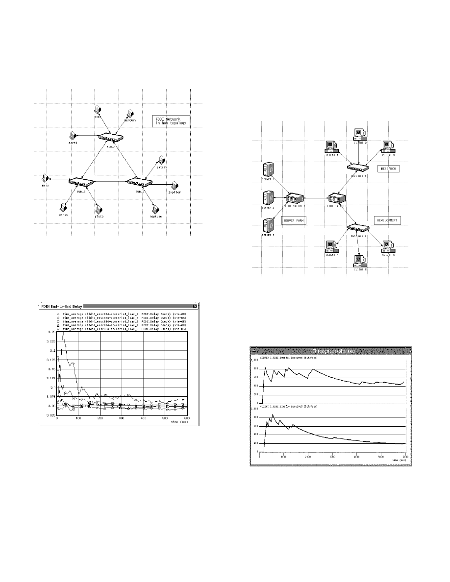
Figure 1. FDDI hub configuration. The network consists
of three concentrators (FDDI hubs) and nine stations.
The concentrators are connected with FDDI duplex links
in a dual-ring topology. The stations are attached to the
ring via concentrators, creating a hub topology.

Figure 2. FDDI end-to-end delay (sec) plots, with traffic
load as a parameter. Load, mean number of frames sent
by the source, according to an exponential distribution,
was varied from 1 to 100 packets per second.

The time-average FDDI end-to-end delay in the network
is shown in Fig. 2. We can observe that, as expected, as
network load increases, end-to-end delay in the network
decreases. We can also observe that the delay appears to

be leveling off with time, which indicates that the
network is stable.

We now consider the second network configuration. Our
goal is to estimate the performance of FDDI network for
one custom application - file transfer protocol (FTP).
The server’s processing speed is 20,000 bytes/sec.
Average file size is set to 15,000 bytes, with 10 file
transfers per hour.

Figure 3. FDDI client-server configuration. This network
topology is suitable for applications such as FTP. Clients
are connected to the network via FDDI hubs. Hubs and
servers at different locations are connected via two
FDDI switches.

Figure 4. Throughput (bits/sec) plots of Server 1 (top)
and Client 1 (bottom).

From Fig. 4 we can observe that the server’s throughput,
once stabilized, is twice as large as the client’s

3

throughput. This is expected because the number of
servers is smaller than the number of served clients in
the network. The leveling of the throughput with time
also indicates a stable network.

3. ATM service categories

In this section we describe simulations of a simple
client-server ATM network, shown in Fig. 5. The
network consists of five ATM clients (each requesting a
different service category), two ATM packet switches,
and one ATM server.

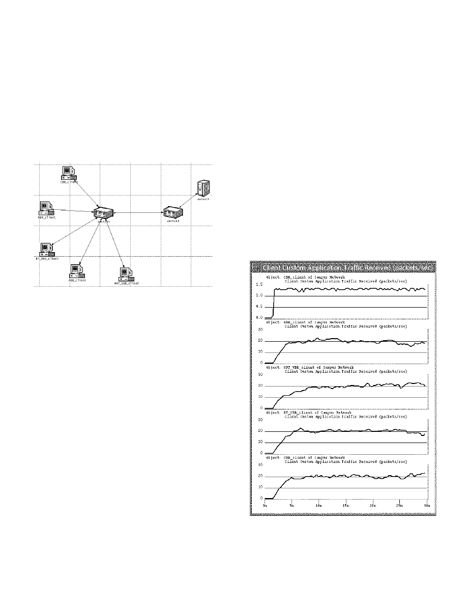
Figure 5. ATM client-server network consisting of two
switches, an ATM server, and five clients requesting five
distinct ATM service categories.

Applications in an ATM network require different
quality of service (QoS) and, therefore, different traffic
categories. For example, a voice application such as a
telephone conversation requires a small transfer delay
not noticeable to the users. However, transfer delay is
not that important for quality video applications with
unidirectional video transfers. In such applications, the
delay jitter (variation in delay) is an important QoS
parameter and should be kept small. The errors and
losses in a voice application or in a video broadcast
might not be very noticeable or important. Nevertheless
for applications such as data transfers, accuracy is
critical. An ATM network has to be able to achieve the
required performance for each of the described
applications. That is the reason that five different service
categories are supported in ATM technology: constant
bit rate (CBR), available bit rate (ABR), real time
variable bit rate (RT_VBR), non-real-time variable bit
rate (NTR_VBR), and unspecified bit rate (UBR) [3].

It is usually difficult to compare and rank the
performance of these five service categories. Each
service category has its own advantages and
disadvantages. CBR and RT_VBR traffic are mostly

deployed for real time applications, such as voice and
video, which put tight constraints on delay and delay
jitter. CBR is, however, more reliable. It guarantees
that, once the connection is set up, the source can emit
cells for any period of time, at any rate lower than or
equal to the peak cell rate (PCR), while upholding the
QoS commitments.

An ATM client-server network with CBR and ABR
clients is available in the OPNET library. In order to
observe the performance of all the service categories, we
have added three more clients. Each client sends request
packets of 1 byte to the server. The request generation
rate is identical for all clients. The connections from the
clients will only be admitted if all the intermediate nodes
in the network can support the requested bandwidth and
QoS. Once a call is admitted, it is routed through the
switches to the server. The server processes the requests
and sends to the clients response packets of 500 bytes.
Traffic patterns received by each client are shown in Fig.
6. As it can be seen, the traffic has a constant bit rate for
the CBR client, and is of a more bursty nature for the
remaining clients.

Figure 6. Traffic received (packets/sec) by CBR, ABR,
NRT_VBR, RT_VBR, and UBR clients (top to bottom)
from the server in the network shown in Fig. 5.

4

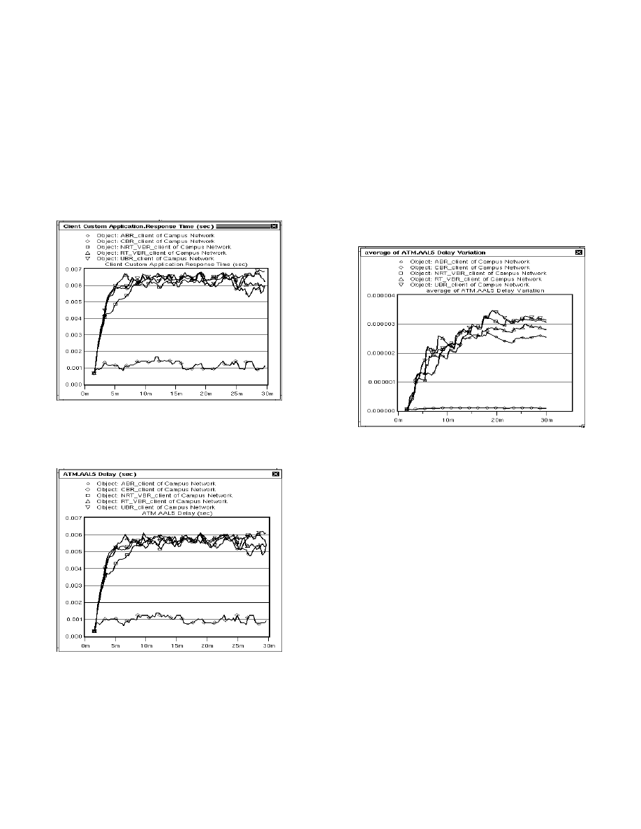
The response time for each of the clients in our network
is shown in Fig. 7. Response time is the time elapsed
between sending a request to the server and receiving a
response. As it can be seen from Fig. 7, the response
time is the smallest for the CBR source. This implies
that CBR delivers the best QoS among the five service
categories we have simulated. The delay and delay jitter
for our simulation scenario are shown in Figs. 8 and 9,
respectively. Again, it can be seen that the CBR client
has the best quality of service because it has the smallest
delay and delay jitter (almost zero). As expected, the
RT_VBR client has the second best delay jitter.

Figure 7. Response time (sec) for each client of Fig. 5.
This is the elapsed time between sending a request
packet to the server and receiving a response from it.

Figure 8. The propagation delay (sec) of packets from
each client to the server shown in Fig. 5.

4. ATM congestion control mechanism

In this section we present the OPNET implementation of
the leaky bucket congestion control algorithm. In ATM

networks, channels do not have fixed bandwidths. Thus,
users can cause congestion in the network by exceeding
their negotiated bandwidth. Prohibiting users from doing
so (policing) is important, because if excessive data
enters the public ATM network without being
controlled, the network may be overloaded and may
encounter an unexpected high cell loss. This cell loss
affects not only the violating connections, but also the
other connections in the network. This degrades the
network functionality. A policing mechanism called
leaky bucket [4, 5] was proposed to remedy this situation
for connections with CBR traffic. A variation called dual
leaky bucket (two concatenated leaky buckets) is used
for policing connections with VBR traffic.

Figure 9. Average delay jitter for different clients of the
network shown in Fig. 5.

4.1 Leaky bucket process model

The leaky bucket mechanism limits the difference
between the negotiated mean cell rate (MCR) parameter
and the actual cell rate of a traffic source. It can be
viewed as a bucket, placed immediately after each
source. Each cell generated by the traffic source carries
a token and attempts to place it in the bucket. If the
bucket is empty, the token is placed and the cell is sent
to the network. If the bucket is full, the cell is discarded.
The bucket gets emptied at a constant rate equal to the
negotiated MCR parameter of the source. The size of the
bucket is equal to an upper bound of the burst length,
and it determines the maximum number of cells that can
be sent consecutively into the network. We have
implemented the leaky bucket by creating a counter in
the OPNET process model. This counter gets
incremented each time a cell is generated by the source.
It gets decremented with a rate equal to the source’s
MCR.

5

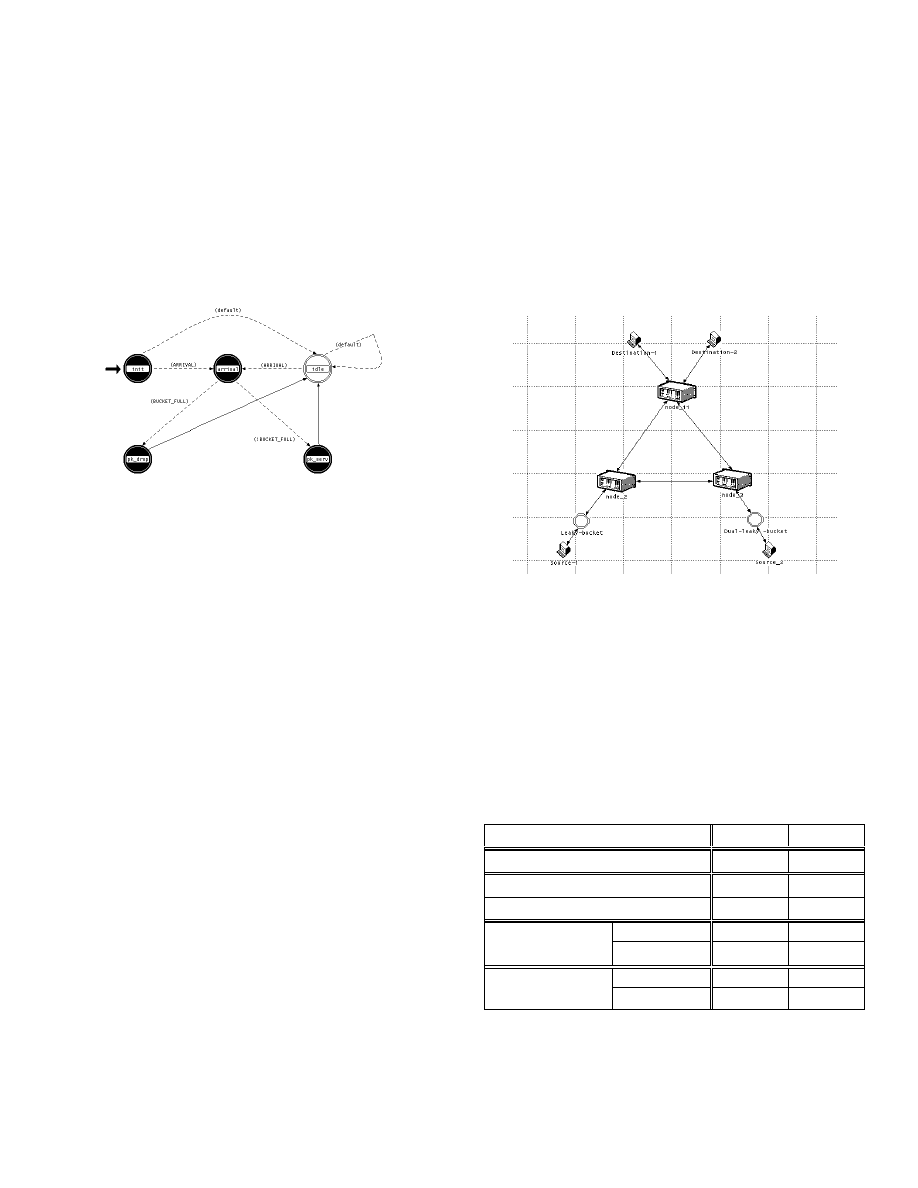
Our leaky bucket process model is shown in Fig. 10. It
contains five states. Starting from initial state, the
process can either reach arrival state when a packet
arrives, or idle state where it remains until the next cell
arrives. From arrival state, the process reaches either
serve or drop state, depending on whether the bucket is
full or empty, respectively.

Users can change the following parameters in the leaky
bucket process model:

-

leaking rate (equal to the negotiated cell rate)

-

bucket size (the upper bound on the burst size).

Figure 10. State transition diagram of the leaky bucket
process model.

Single leaky bucket is used to police CBR traffic. Since
MCR is the only parameter negotiated with the network
for this type of traffic, single leaky bucket is designed to
monitor the MCR parameter.

We implement a dual leaky bucket mechanism by
concatenating two leaky bucket process models. This
mechanism may be used to police VBR sources. In VBR
traffic, both MCR and PCR traffic parameters need to be
policed [5]. The first and the second bucket’s leaking
rates are set to the PCR and MCR of the source,
respectively. Cells are discarded when one of the two
leaky buckets has reached its threshold value.

The leaky bucket OPNET process model, named “leaky
bucket”, has been deposited into the OPNET
Contributed Model Depot [6]. This process model is
then used to create single and dual leaky bucket node
models.

4.2 ATM network model

In order to illustrate the functionality of leaky bucket
mechanisms, we model a small ATM network shown in
Fig. 11. Sources 1 and 2 have negotiated CBR and VBR
traffic, respectively. However, the sources are not
conforming to their negotiated traffic contract and the

actual traffic they send has a higher rate than their
contract. Therefore, leaky buckets are used to police
these sources. The negotiated MCR and PCR of the
sources, as well as the bucket size and the leaking rate of
the leaky buckets are shown in Table 1.

Source-1 is policed by a single leaky bucket mechanism
with leaking rate equal to the negotiated MCR. We
choose the bucket size by taking into account that the
size should be selected as small as possible in order to
limit the full-rate bursts allowed into the network.
Nevertheless, we keep the size reasonably large, because
a very small bucket size causes cells from conforming
sources to be discarded.

Figure 11. ATM network model. The model consists of a
CBR and a VBR ATM source, three ATM switches, and
two destinations. A leaky bucket process model is used
for each source.

A dual leaky bucket is used to police Source-2. The
leaking rate of the first leaky bucket is equal to the
negotiated PCR of the VBR traffic source. Its bucket
size is chosen according to both PCR and delay jitter
parameters of the connection. The leaking rate of the
second bucket is equal to the MCR negotiated by the
source. Its bucket size is the maximum burst accepted by
the network.

Table 1. Traffic rate and leaky bucket parameters set in
the network of Fig. 11.

Source-1 Source-2

Traffic type

CBR

VBR

Negotiated MCR

2

1

Negotiated PCR

-

2

leaking rate

2

2

Leaky bucket 1

bucket size

30

60

leaking rate

-

1

Leaky bucket 2

bucket size

-

40

6

4.3 Simulation results

We are interested in the performance of the leaky bucket
mechanism when used to police misbehaving sources.
During simulation, we collect the number of packets that
are discarded by leaky bucket and observe the burst size
allowed into the network. The burst size is equal to the
number of free spaces in the bucket at each instance. It
can be calculated by subtracting the number of bucket
spaces occupied by tokens from the bucket size.

Figure 12. Single leaky bucket: Burst size (cells)
allowed into the network (top). Number of lost cells
(bottom).

Fig. 12 (top) shows that the size of the burst entering the
network is limited by the bucket size (30 cells). The
number of lost cells from Source-1, after it has been
policed, is shown in Fig. 12 (bottom). This number is a
function of the leaking rate (MCR) and the bucket size.
Fig. 13 illustrates the performance of the dual leaky
bucket. The number of lost cells is a function of the
leaking rates: PCR for the first and MCR for the second
bucket.

(a)

(b)

Figure 13. Dual leaky bucket: The burst size (top), the
number of tokens in the bucket (middle), and the number
of lost cells (bottom) for the first (a) and second (b)
leaky bucket.

5. Conclusions

In this paper we focused on simulating two commonly
used packet data network technologies: FDDI and ATM.
We simulated two FDDI and two ATM network
scenarios. Our major contribution is modeling the leaky
bucket congestion control mechanism for ATM
networks. The model is available from the OPNET
Contributed Model Depot.

References

[1] ANSI X3.139-1987: Fiber Distributed Data Interface
(FDDI) - Token Ring Media Access Control (MAC)
http://www.ansi.org.
[2] I. Katzela and Mil 3, Inc., Modeling and Simulating
Communication Networks: A Hands-on Approach Using
OPNET, Upper Saddle River, NJ, Prentice Hall, 1999,
pp. 91-102.
[3] ATM Forum. Traffic Management Specification
Version 4.0 ftp://ftp.atmforum.com/pub/approved-specs/
af-tm-0056.000.pdf.
[4] E. P. Rathgeb and T. H. Theimer, “The policing
function in ATM networks,” Proceeding of the
International Switching Symposium, Stockholm,
Sweden, June 1990, vol. 5, pp.127-130.
[5] G. Niestegge, “The leaky bucket policing method in
asynchronous transfer mode networks,” International
Journal of Digital and Analog Communication Systems,
vol. 3, pp. 187-197, 1990.
[6] OPNET Contributed Model Depot:
http://www.opnet.com/services/depot/home.html.