
EXTRACTION OF ALCOHOLS FROM GASOLINE
USING SOLID PHASE MICROEXTRACTION (SPME)
Iris Stadelmann
Thesis submitted to the faculty of the
Virginia Polytechnic Institute and State University
in partial fulfillment of the requirements for the degree of
MASTER OF SCIENCE
In
Chemistry
Dr. Harold M. McNair, Chair
Dr. Herve Marand
Dr. Larry T. Taylor
May 11, 2001
Blacksburg, Virginia
Key words: GC, SPME, Sample preparation, Gasoline
Copyright 2001, Iris Stadelmann

EXTRACTION OF ALCOHOLS FROM GASOLINE USING SPME
By
Iris Stadelmann
(Abstract)
It is common practice to add oxygenates, such as ethers or alcohols, to gasoline in
areas suffering from ozone or smog problems in order to reduce pollution. The most
commonly used oxygenates are ethanol (EtOH) and methyl tert-butyl ether (MTBE).
However, MTBE is now forbidden by the environmental protection agency (EPA)
because of the possibility of ground water contamination. The current trend is to use
EtOH, therefore this work focuses on the analysis and quantification of EtOH in gasoline
by solid phase microextraction (SPME). The major problem in quantifying EtOH in
gasoline is the coelution of hydrocarbons with EtOH. There have been several
approaches to solve this problem; among the chromatographic ones, three major types
have been proposed: (1) the first one uses a detector selective for oxygen containing
compounds; (2) the second one uses two or more columns; (3) and the third one uses an
extraction step prior to GC analysis. In this work an extraction step with water is used
prior to a solid phase microextraction (SPME) sample preparation coupled to a gas
chromatographic (GC) analysis.
Solid phase microextraction is a recent technique, invented by Pawliszyn in 1989,
and available commercially since 1994. A fiber is used to extract small amounts (ppm,
ppb, ppt) of analytes from a solution, usually water. The fiber is beneficial in
concentrating analytes. Most work using SPME has been done with hydrophobic (non
polar) analytes, extracted using a polydimethylsiloxane (PDMS; non polar) coating on a
fused silica fiber. Since very little work has been done with polar analytes, the novel
approach of this work is the extraction of EtOH.
Since EtOH is the analyte of interest, a polar fiber, carboxen/polydimethyl
siloxane (Car/PDMS) is used. Two methods are used for quantification of EtOH in

iii
gasoline: the method of a standard calibration curve, and the method of standard addition.
They are both successful in quantifying the amount of EtOH in gasoline. The relative
errors, with the method of standard addition, vary from 5.3% to 14%, while the ones with
the method of calibration curve vary from 1.6% to 7.2%. Moreover, some extraction time
studies for both direct and headspace sampling are performed. Direct sampling shows the
presence of an equilibrium condition for the carboxen/PDMS fiber, for which no
extraction theory is available. Conversely, headspace sampling shows no equilibrium
state; after a sampling time of one hour, the amount of EtOH extracted decreases with
sampling time. This is probably due to displacement of EtOH by other compounds in the
fiber.

iv
ACKNOWLEDGEMENTS
I would like to thank my advisor, Dr. Harold McNair, for his knowledge and
guidance. I would also like to thank my committee members, Dr. Herve Marand and Dr.
Larry Taylor, for reviewing my thesis and giving me some good comments and
suggestions.
Thanks to the chemistry department for providing me a teaching assistantship
during my graduate studies.
Thanks to my group members for the pleasant lab environment, help, friendship
and technical knowledge. Special thanks to Dr. Yvonne Fraticelli, who gave me some
helpful suggestions in my research, to Jennifer Brown and Laura Nakovich, always
friendly and ready to help, to the usual or occasional “evening lab buddies”, who brought
life to the lab at night, to Kevin Schug, Arash Kamangepour, and Amy Kinkennon.
Thanks also to the “older” lab members who graduated some months ago, especially
Gail, Mark, and Xiling.
Thanks to my chemistry buddies, those who came in with me as well as the other
ones, especially Paco, Brian, Emre, Lee, and Luis. Special thanks to Paolo Dadone,
Aysen Tulpar, and Christos Kontogeorgakis, for their great friendship and personalities.
Paolo’s argumentative nature made for interesting and helpful discussions.
I would also like to thank my old and new friends, as well as my family, for their
love and support, and especially my parents Victor and Elizabeth, who made all this
possible.

v
Table of contents
ACKNOWLEDGEMENTS .........................................................................................iv
TABLE OF CONTENTS ..............................................................................................v
LIST OF FIGURES.....................................................................................................vii
LIST OF MULTIMEDIA OBJECTS ..........................................................................ix
CHAPTER 1- INTRODUCTION............................................................................ 1
1.1.1 History................................................................................................................1
1.1.2 Advantages and disadvantages ............................................................................2
1.1.3 Gasoline components ..........................................................................................5
CHAPTER 2 - SOLID PHASE MICROEXTRACTION........................................ 11
2.1 Introduction ...........................................................................................................11
2.3 Theory ....................................................................................................................15
2.3.1 Determination of amount of analyte extracted at equilibrium (thermodynamics)16
2.3.2 Dynamic process (kinetics) of direct SPME ......................................................20
2.3.3 Dynamic process (kinetics) of headspace SPME ...............................................21
CHAPTER 3 - EXPERIMENTAL SETUP AND METHODS................................ 25
3.2.1 Gasoline samples ..............................................................................................27
3.2.2 Mixing procedure..............................................................................................28
3.2.3 SPME conditions ..............................................................................................29

vi
3.3 GC conditions ........................................................................................................30
3.4 Data analysis ..........................................................................................................31
3.4.1 Method of calibration curve ..............................................................................32
3.4.2 Method of standard addition..............................................................................32
3.5 Salt addition ...........................................................................................................34
CHAPTER 4 - RESULTS AND DISCUSSION .................................................. 35
4.1 Linearity curves .....................................................................................................35
4.3 Standard addition curves ......................................................................................42
CHAPTER 5 – CONCLUSIONS......................................................................... 51

vii
LIST OF FIGURES
Figure
Description
Page
12
13
14
16
17
25
26
26
36
(F.I.D.) 37
37
38
38
SPME-GC of 39 ppm EtOH in the water extracted gasoline fraction
39
SPME-GC of 4.3 ppm EtOH in the water extracted gasoline fraction
40
curve 41
curve 42
44
46
47
48
49
50

viii
LIST OF TABLES
Table
Description
Page
Common components of gasoline, and some of
Twenty major components of API PS-6
7
Relation between oxygenate amounts and volumes
27
28
Regular unleaded gasoline water solubility
28
Data set 1, using 5.7 wt.% EtOH stock solution
44
Data set 2, using 6.6 wt.% EtOH stock solution
Data set 3, using 6.6 wt.% EtOH stock solution
47

ix
LIST OF MULTIMEDIA OBJECTS
Multimedia Description
Page
Object
12
13

1
CHAPTER 1 - INTRODUCTION
1.1 Background
1.1.1 History
For different reasons, it is very common to put additives in gasoline. Among those
additives, oxygenates are commonly used in order to increase the amount of oxygen
contained in gasoline. The oxygenates that are added can be either ethers (e.g., methyl
tert butyl ether (MTBE), ethyl tert butyl ether (ETBE), and tert amyl methyl ether
(TAME)) or alcohols (e.g., methanol (MeOH) and ethanol (EtOH)) [51]. Additives are
chosen based on their cost and octane enhancing capabilities [50,58]. In the 1920s,
MeOH and EtOH were already known to be octane enhancers, reducing knocking and
allowing smoother burning [29,33,63]. They started being widely used since octane
numbers in those days were quite low, therefore an improvement in engine performance
by adding alcohols could easily be noticed. Lead additives started being substituted for
alcohols since they were better octane enhancers, however they were banned in 1996
because they were major sources of lead contamination [33]. Therefore, the use of
alcohols resurfaced.
Crude oil prices also influence the amount of oxygenates added to gasoline.
Indeed, if crude oil prices are high, then it is more economical for the fuel blender to
add oxygenates. For example, in the 1970s, during a period of oil crisis, gasoline
supplies were restricted, and therefore more oxygenates were used as gasoline
supplements. Up to 10 % alcohol was added to gasoline, yielding what became known
as gasohol [54].
Methanol has been used in high concentration, in Canada, in specially designed
cars, employing a specifically designed engine (“M85 fuel flexible vehicles”) [55].
Those cars can run with a gasoline mixture containing up to 85% MeOH. A minimum
of 15% gasoline is required, in order to not only facilitate engine start during cold

2
weather, but also to add more safety to the whole blend. Indeed, MeOH burns with a
flame that is almost invisible in the daylight; thus, an ignited fuel spill would barely get
noticed. On the contrary, gasoline burns with a yellow flame, thus making the whole
blend flame more visible [55].
Currently, the Clean Air Act Amendments of 1990 require the addition of oxygen
to gasoline in areas suffering from ozone or smog problems in order to reduce pollution
[58]. Such a reformulated gasoline (RFG) has to contain at least 2% oxygen by weight
during the year and at least 2.7% oxygen by weight during the wintertime [62]. The
most commonly used oxygenates are EtOH and MTBE. However, MTBE is now
almost forbidden by the environmental protection agency (EPA) because of the
possibility of ground water contamination [14,57,61,62]. Indeed, MTBE has been
known to leak into drinking water sources from underground gasoline storage tanks,
causing a complex problem because it is very difficult to remove it from water [57].
Even though this theory has been challenged by an MTBE producer [60], the current
trend is to use EtOH, which is highly biodegradable and therefore will unlikely travel
far from spills or leaks [38,57].
1.1.2 Advantages and disadvantages
The addition of oxygenates to gasoline offers many advantages, among which:
•
more complete combustion and reduction of carbon monoxide emissions;
•
being a renewable energy source;
•
increased octane number;
•
increased volatility.
Most importantly, the use of RFG reduces air toxic emissions and CO emissions,
therefore reducing pollution emissions that cause ground level ozone problems
[3,15,21,39,47,58]. Indeed, the addition of oxygenates allows a more complete
combustion in the transient operation of the car. Furthermore, in the steady operation of
the car, it shifts the reaction equilibrium to CO
2
rather than CO [21,51]. During engine

3
start or during vehicle acceleration (i.e., transient operation), an excess of gasoline is
present in the burning chamber. This causes a lower oxygen-to-gasoline ratio, resulting
in an incomplete combustion causing higher hydrocarbon emissions since there is not
enough oxygen to burn all the gasoline hydrocarbons. Adding oxygenates increases the
oxygen-to-gasoline ratio (i.e., “richer” gasoline-air mixture, richer in oxygen), which
results in a more complete combustion [2,22]. During steady engine operation, the
oxygen-to-gasoline ratio is the stoichiometric one (“normal” gasoline-air mixture).
Adding oxygenates to the mixture produces an excess of oxygen and the reaction
equilibrium is shifted towards CO
2
rather than CO. The addition of oxygenates also
allow faster and more stable combustion.
The addition of oxygenates to gasoline is beneficial in reducing the dependency
from non-renewable energy sources. Indeed, oxygenates can be produced from
available sources (e.g., biomass, sewage, municipal and agricultural waste)
[9,17,27,28,44,45,46,56], whereas oil, a natural (non-renewable) energy source, cannot.
Methanol, also known as “wood alcohol”, can be either obtained by distillation of
wood (oldest process), or produced synthetically using natural gas, coal gas, water gas
or sewage gas at high temperature and pressure and in the presence of metallic
catalysts, as follows [29]:
CO
+
2H
2
→
−
C
O
Cr
ZnO
o
400
,
3
2
CH
3
OH (1)
Ethanol, also known as “grain alcohol”, can be produced naturally from the
fermentation of fruit juices, vegetable matter, and carbohydrates [29]. The ethanol
hence produced, called “bio-ethanol”, is wet, and therefore needs to be further distilled
to remove excess water and to be purified. The fermentation reaction is as follows:
C
6
H
12
O
6
→
yeast
2C
2
H
5
OH + 2CO
2
(2)
Ethanol can also be produced synthetically, by a hydration reaction of ethylene, as
follows [29]:
CH
2
==CH
2
→
4
2
SO
H
CH
3
CH
2
OSO
2
OH
→
heat
O
H
,
2
CH
3
CH
2
OH
(3)
Methyl tert butyl ether, can be produced in different ways, each having a common
final step which is a reaction of methanol with isobutylene [29]:
(CH
3
)
2
C == CH
2
+ CH
3
OH
(CH
3
)
3
COCH
3
(4)

4
Oxygenates have a high octane number, therefore their addition to gasoline
enhances the octane number of the gasoline mix, therefore reducing “knocking” in the
engine [9,53]. If the octane number is already at the desired level, then it is possible to
reduce the amount of other high octane compounds, like aromatics, which are
sometimes toxic (e.g. benzene, toluene, xylene), and add more oxygenates to keep the
same overall octane number.
Since they increase volatility, and thus allow for an easier engine start, oxygenates
are added to gasoline in higher quantity during the wintertime. Indeed, gasoline needs
to be mixed with air (vaporized) in order to burn in the engine, and thus it needs to be
volatile. At low temperatures, gasoline vaporizes less easily, which can result in car
stumbling or hesitating and slower engine warm-up [29]. Increased volatility of RFG is
mostly true when alcohols are used. Indeed, MTBE only slightly increases the blend’s
volatility, and ETBE and TAME do not increase the blend’s volatility [49].
There are also disadvantages in adding oxygenates to gasoline, among which:
•
corrosion;
•
lower energy content;
•
increased cost;
•
phase separation;
•
increased volatility.
Especially in older engines, oxygenates can soften hoses and gaskets [54], and
dissolve plastic parts [51]. Moreover, they can also corrode metal with different
intensities, as follows: MeOH > EtOH > MTBE [29].
Oxygenates have a lower energy content than gasoline, thus reducing the fuel
efficiency of RFG. For example, the addition of 10 volume % EtOH reduces the fuel
efficiency by only a few percents. Indeed, the combustion of EtOH releases 76,000
British thermal units (Btu) per gallon, while the combustion of conventional gasoline
releases 115,000 Btu per gallon. The combustion of RFG with 10 volume % EtOH
releases only 111,100 Btu per gallon.

5
When the oil prices are not peaking, the cost of RFG increases because of the
addition of oxygenates. So, unless there is a tax exemption for using oxygenates (and/or
they are required by law), they will not likely be added [49].
When water is present in the gasoline, phase separation can occur if alcohols are
the oxygenates used, since alcohols are very water soluble and would move to the
bottom water phase. The top (alcohol deficient) gasoline phase would then have a lower
octane number and may cause an engine to knock. Because of this problem, gasoline
oxygenated with alcohols is not transported in pipelines, which sometimes contain
water [49]. This problem is not seen with MTBE [51].
Finally, the increased volatility can lead to vapor lock in hot weather or high
altitude [54]. Gasoline can vaporize in the fuel system and prevent the fuel pump from
delivering sufficient gasoline to the engine. This would result in loss of power or engine
shutdown [51].
1.1.3 Gasoline components
Gasoline is a very complex mixture, containing hundreds of different compounds.
Those compounds can be divided into three classes:
•
aliphatic compounds (poorly water soluble);
•
aromatic compounds (moderately water soluble);
•
oxygenated compounds (optional; alcohols highly water soluble).

6
A list of some of these common gasoline components, along with some of their
physical properties, is shown in Table 1.1. An example of standard gasoline
composition is shown in Table 1.2.
Table 1.1: Common components of gasoline, and some
of their physical properties
Compound
MW
b.p.
v.p.
water
(
°°°°
C)
(mmHg) solubility
(@
20oC)
(mg/L)
AROMATIC
benzene 78
80.1
76
1780
COMPOUNDS
toluene 92
110
22
515
o-xylene 106
144.4
5
175
m-xylene 106
139.1
6
_
p-xylene 106
138.4
6.5
198
ethylbenzene 106
136.2
7
152
ALIPHATIC
methane 16
-161
gas
24
COMPOUNDS
ethane 30
-88.6
_
60.4
n-propane 44
-42.1
_
_
n-butane 58
-6.2
1823
61
n-pentane 72
30
430
_
n-hexane 86
68.7
120
9.5
n-heptane 100
98.4
35
3
n-octane 114
125.5
11
0.66
trimethyl-pentanes 114 99
_
0.56
OXYGENATED methanol 32
64.7
92
miscible
ADDITIVES
ethanol 46
78.5
43.9
miscible
methyl-t-butylether 88 252 252 miscible

7
1.2: State of the Art
The discussion in the previous section (Section 1.1) shows the need to quantify
oxygenates in gasoline. First of all, there is a need to quantify them during the blending
of gasoline for quality assurance and process control purposes. Second, there is a need
to quantify them during the delivery of gasoline, for example at gasoline stations, to
check the accuracy of blenders’ claims (e.g., consumers’ associations, regulatory
agencies), and also to check for possible contaminations [52].
The main problem encountered in performing a gas chromatographic analysis of
oxygenates in gasoline is the coelution of aliphatic compounds with oxygenates, which
leads to difficult quantification.
Table 1.2: Twenty major components of API PS-6 unleaded gasoline
(American Petroleum Institute, Washington D.C., 1988)
COMPONENT Percent
Weight
Aqueous
Solubility
(API,
1985)
(mg/L)
2-methylbutane 8.72
49.6
m-xylene 5.66
185
2,2,4-trimethylpentane 5.22
2.4
toluene 4.73
554
2-methylpentane 3.93
15.7
n-butane 3.83
61.4
1,2,4-trimethylbenzene 3.26
57
n-pentane 3.11
47.6
2,3,4-trimethylpentane 2.99
2.3
2,3,3-trimethylpentane 2.85
2.6
3-methylpentane 2.36
17.9
o-xylene 2.27
175
ethylbenzene 2
161
benzene 1.94
1780
p-xylene 1.72
156
2,3-dimethylbutane 1.66 22.5
n-hexane 1.58
12.4
1-methyl,3-ethylbenzene 1.54
40
1-methyl,4-ethylbenzene 1.54
40
3-methylhexane 1.3 5

8
There have been several approaches taken to quantify oxygenates in gasoline,
either using chromatographic techniques, or using other types of techniques, like
spectroscopy. The chromatographic approaches can be subdivided into three main
categories, based on the way they try to solve the coelution problem. Namely there are:
•
approaches using two or more columns [16,52,59];
•
approaches using a selective detector for oxygen containing compounds
[10,11,12,18,43];
•
approaches using an extraction step prior to chromatographic analysis [1,26,34].
The first two classes of approaches present the main problem of requiring specific
instrumentation.
The standard test method for quantification of low molecular weight alcohols
(such as methanol and ethanol) and MTBE in gasoline is the ASTM-D4815. This
method uses two columns and a column switching valve [59]. The sample first goes
through a polar column in order to eliminate the light non polar compounds (these go to
vent). Then the valve is switched in order to have the remainder of the sample go
through the second column and be measured. This column is non polar, so that alcohols
and MTBE elute before the heavier hydrocarbons. Finally, the valve is switched back to
its original position to backflush the heavy hydrocarbons. This is a complicated method
and it requires specific hardware.
The ASTM method is one of the two methods currently used by the EPA for
quantification of alcohols in gasoline [52]. The other method uses a water extraction
step in order to eliminate hydrocarbon interferences, followed by chromatographic
analysis of the water sample. Calibration standards are used, along with an internal
standard (isopropanol) added to the gasoline before the extraction step, in order to
quantify the amount of alcohols in gasoline [52].
Frysinger and Gaines [16] have quantified oxygenates using two-dimensional gas
chromatography. Two columns are used in order to get better resolution. The first
column separates compounds based on their volatility, while the second one separates
compounds based on their polarity. The chromatogram obtained is a 2-D retention time
plane with analytes organized by volatility and polarity properties.

9
Kanai et al. [26] have analyzed MTBE, ETBE, and TAME in gasolines by
GC/MS. They used an acetonitrile (ACN) extraction step to remove hydrocarbon
interferences. They mixed ACN with gasoline in a separatory funnel, and shook the
mixture for 5 minutes. Three layers formed after the addition of saturated sodium
chloride: a top hydrocarbon layer, a middle ACN layer (containing most of the ethers),
and a bottom aqueous layer. The top and bottom layers were discarded. The middle
layer was passed through a disposable pipette fitted with glass wool to remove any
residual water. Then the sample was heated for 25 minutes to eliminate the small
amounts of hydrocarbons present. The volume of the final sample was measured and
the sample analyzed by GC-MS. They used an internal standard to quantify the ethers;
their interference removal technique was successful in removing the hydrocarbon
interferences, however it led to a very poor recovery (12% recovery).
Agarwal [1] used diethylene glycol to extract low molecular weight alcohols from
gasoline in order to quantify them by GC, by eliminating hydrocarbon interferences. He
used propanol as an internal standard. His method had the disadvantage of using an
organic solvent.
Pauls and McCoy [34] used a water extraction step before a GC analysis using a
packed column and isopropanol as an internal standard. The disadvantage of their
method is the introduction of water inside the GC column, which results in a shorter
column lifetime.
Among the approaches using oxygen selective detectors, Verga et al. [43] and Di
sanzo [12] used an oxygenates FID (O-FID) analyzer. Diehl et al. [11] used an atomic
emission detector (AED) on a GC instrument. Diehl et al. [10] used a Fourier transform
infrared (FTIR) spectroscope as a GC detector. Goode and Thomas [18] used a
microwave-induced plasma (MIP) GC detector. These approaches all require
chromatographic instrument modification.
Finally, some non-chromatographic methods have also been used to quantify
oxygenates in gasoline. Choquette et al. [8] used Fourier transform near-infrared and
Fourier transform raman spectroscopy. They showed that their technique was capable
of quantifying four common oxygenate additives (MTBE, ETBE, TAME, and EtOH) in
single-oxygenate gasoline mixtures, however they could achieve accurate quantification

10
only in well known and fixed neat-fuel composition. Sarpal et al. [40] have analyzed
oxygenates in gasoline using
13
C NMR spectroscopy. Skloss et al. [42], Kalsi et al.
[25], and Meusinger [32], have used
1
H NMR to analyze oxygenates in gasoline. Fodor
et al. [13] and Iob et al. [23] have used FTIR spectroscopy.
A different approach to eliminating hydrocarbon interferences consists in using
solid phase microextraction (SPME). The details of SPME will be discussed in the
following chapter (Chapter 2). However, SPME uses a fiber for extracting analytes and
this could be helpful in filtering some of the hydrocarbons. Gorecki et al. [20] have
analyzed methanol, ethanol, and 2-propanol in unleaded gasoline and water using
SPME. They used a custom made polar fiber, coated with Nafion perfluorinated resin.
This fiber extracts analytes by adsorption and allowed good quantification of MeOH,
but did not allow good quantification of ethanol and 2-propanol in water. Their work
does not explain the details of the technique and only proves detection but no
quantification of either MeOH or EtOH. They observed a non-linear response of
analyte amounts extracted with this fiber at long sampling times. Indeed, since the
coating surface has a limited number of adsorption sites, analytes with a lower affinity
for the fiber are eventually displaced by the other analytes. They achieved better
linearity by using two different experimental settings. The first one consisted in using a
short extraction time with vigorous stirring; the second one consisted in using an
extraction time for which some analytes did not reach equilibrium, with no stirring.
In this work we will quantify the amount of EtOH in gasoline using a combination
of a water extraction step along with SPME-GC analysis. Our proposed method does
not require specific instrumentation like in the multiple columns [16,52,59] and
selective detector [10,11,12,18,43] cases. It also eliminates the use of organic solvent
like in [1] and [26], and avoids the insertion of water inside the GC (detrimental to the
column) like in [34].
In the following chapter we will provide some background information about
SPME, and in Chapter 3 we will describe the experimental setup and methods. In
Chapter 4 we will discuss our results, and finally we will conclude our work in Chapter
5.

11
CHAPTER 2 - SOLID PHASE MICROEXTRACTION
2.1 Introduction
Sample preparation is often a long and tedious process, and a time limiting factor
in the analysis of compounds. Indeed, on average, two-thirds of the analysis time in
chromatography is spent on sampling and sample preparation steps and only one-third
on the analysis itself! Moreover, 90% of high performance liquid chromatography
(HPLC) and gas chromatography (GC) users use two or more preparation techniques
per sample. Therefore, it is important to minimize sample preparation time and
optimize the efficiency of those steps. Solid Phase MicroExtraction is a quick sample
preparation technique, where usually no other sample preparation step is required,
hence minimizing the sample preparation time and the chance for error.
In the remainder of this chapter, we describe in detail the SPME technique
(Section 2), the theory (Section 3) and the fibers (Section 4).
2.2 Technique
SPME is a recent technique, invented by Pawliszyn in 1989 [6] and available
commercially since 1994. A fiber is used to extract small amounts (ppm, ppb levels) of
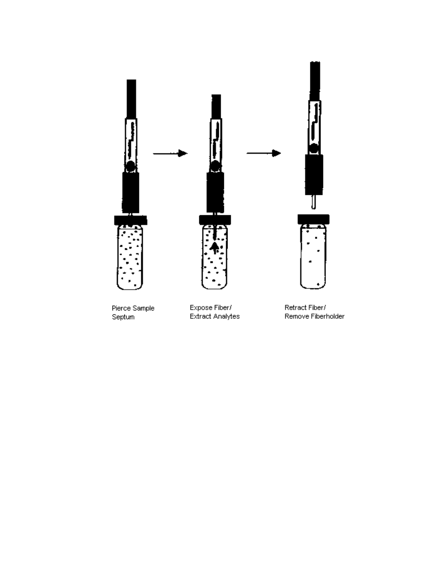
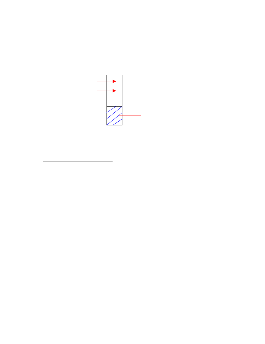
analytes from a solution, usually water. This technique is composed of two steps [31].
First, an extraction step (illustrated in Fig. 2.1), where analytes get sorbed onto the fiber
and extracted from the solution or the headspace. Then, a desorption step (shown in
Fig. 2.2), during which analytes are thermally desorbed into a heated GC injection port.
12
The extraction step can be subdivided into three substeps. First, the sample vial
septum is pierced by a septum piercing needle. Since the fiber is very fragile, the
purpose of the septum piercing needle is to protect the fiber. After the septum is
pierced, the fiber is exposed to the solution, either directly (i.e. direct sampling) or in its
gas phase (i.e. headspace sampling). This allows the analytes from the solution to
diffuse into the fiber. After a fixed amount of time the fiber is retracted inside the
septum piercing needle, and the fiber holder (Fig. 2.3) is remov ed from the solution.
Click here to see an animation of the extraction step (28.6KB)
Fig. 2.1: Extraction step
13
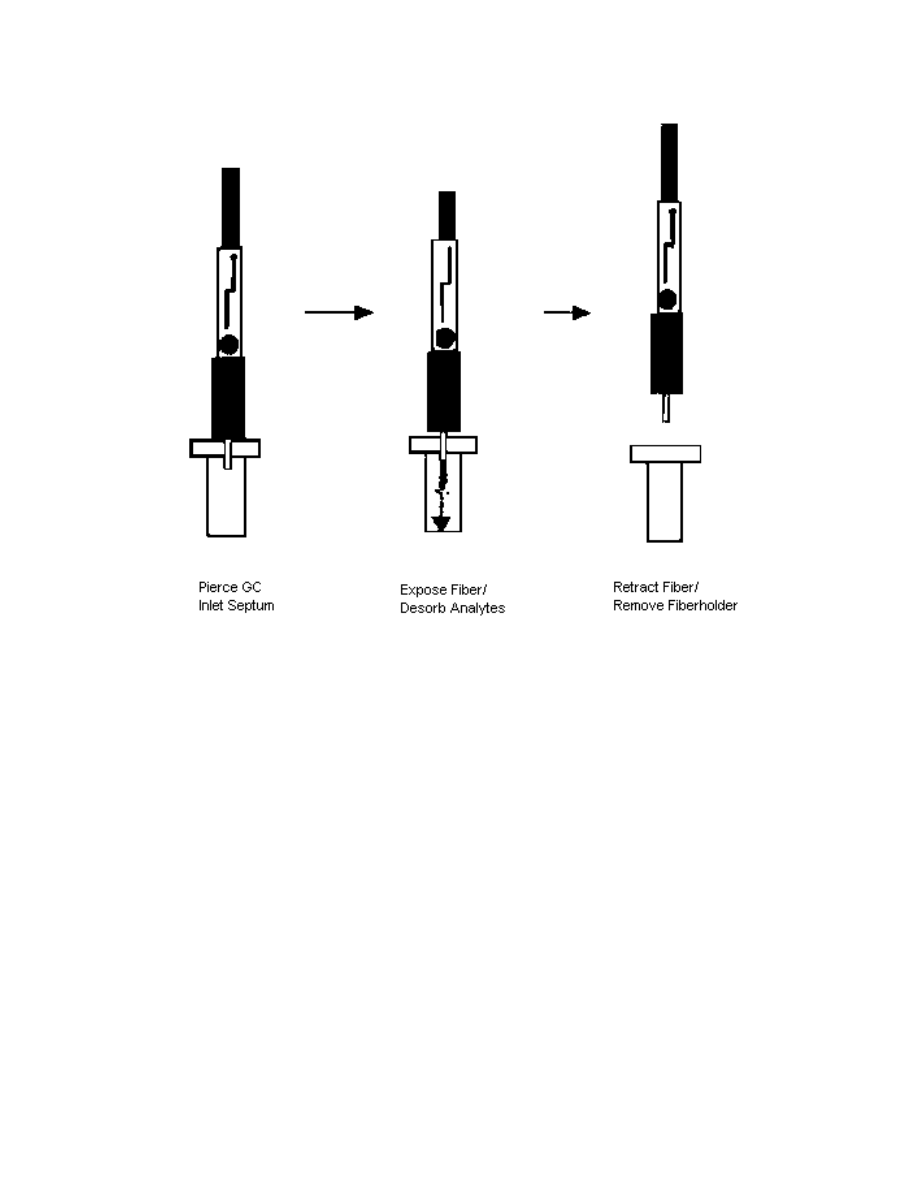
The desorption step is also composed of three substeps. First, the GC inlet septum
is pierced with the septum piercing needle. Then the fiber is exposed to the hot GC
injection port, where the analytes are thermally desorbed. The fiber is left in the GC for
a few minutes in order to allow complete desorption and cleaning. The fiber is finally
retracted inside the septum piercing needle and the fiber holder is removed from the GC
injection port.
Click here to see an animation of the desorption step (43.6KB)
Fig. 2.2: Desorption step
14
SPME offers many advantages over other sample preparation techniques
[36,48,64]:
•
it is organic solvent free;
•
it is low cost (in the order of hundreds of dollars);
•
it is highly sensitive (analytes down to the ppm, ppb, and sometimes ppt levels can be
detected [37]);
•
it uses short extraction time (in the order of minutes);
•
it is easy to use;
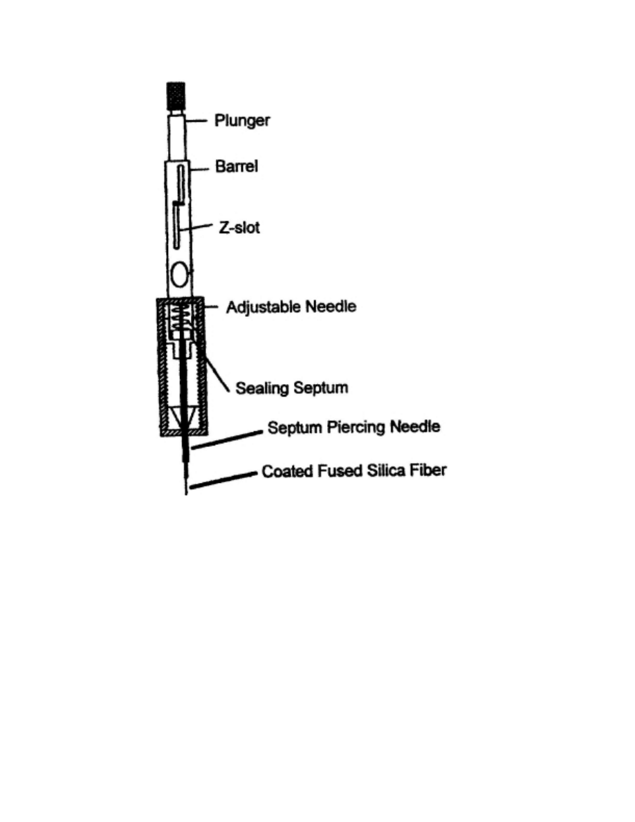
Fig. 2.3: Scheme of SPME assembly

15
•
it often does not require any other sample preparation step;
•
it can easily be automated;
•
it allows field sampling: sample the analytes on-site with a portable field sampler,
then bring the capped fiber back to the lab for the actual analysis.
However there are two main disadvantages to this technique:
•
it is limited to aqueous samples;
•
it cannot be used for highly concentrated analytes.
SPME was originally used for trace analysis of impurities in water
[4,5,7,24,30,31,36,37,]. Lately it has also been used in pharmaceutical, environmental,
foods and flavors, forensic, and toxicology applications [36,48,64]. Most work has been
done with hydrophobic (non polar) analytes, extracted using a polydimethyl siloxane
fiber (PDMS; non polar fiber, most widely used). Since very little work has been done
with polar analytes [20], the novel approach of this work consists in extracting polar
analytes (MeOH, EtOH).
2.3 Theory
Two mechanisms are possible, according to the nature of the fiber. If the fiber is a
liquid phase, the analytes are extracted by absorption; if the fiber is a porous particle
blend, the analytes are extracted by adsorption. Absorption is a non-competitive process
where analytes dissolve into the bulk of the liquid, whereas adsorption is a competitive
process where analytes bind to the surface of the solid [19]. In the adsorption case,
there is a limited number of sites where analytes can bind to. When all the sites are
occupied, the fiber is saturated. Therefore the linear range of adsorption-type fibers is
smaller than the one for absorption-type fibers. In a competitive process, analytes of
higher affinity for the coating can displace analytes of lower affinity for the fiber.
In this section we will explain some of the theory behind the use of SPME. We
will first start by analyzing the equilibrium process (thermodynamics) [35], and then
consider the dynamics that lead to equilibrium (kinetics) [2]. The thermodynamic and
kinetic expressions are derived for the absorption mechanism only. The thermodynamic
16
expression for most of the adsorption-type fibers is similar to the one for absorption-
type fibers, and the same conclusion is valid, if a sufficiently dilute solution is used.
The carboxen/PDMS fiber is an exception, and no extraction model has been developed
for it so far [19]. Indeed, this fiber has pores small enough to cause capillary
condensation, which can result in a higher extraction capacity of the fiber for some
analytes [19]. However if the analytes concentrations are low enough, capillary
condensation is negligible [19].
2.3.1 Determination of amount of analyte extracted at equilibrium
(thermodynamics)
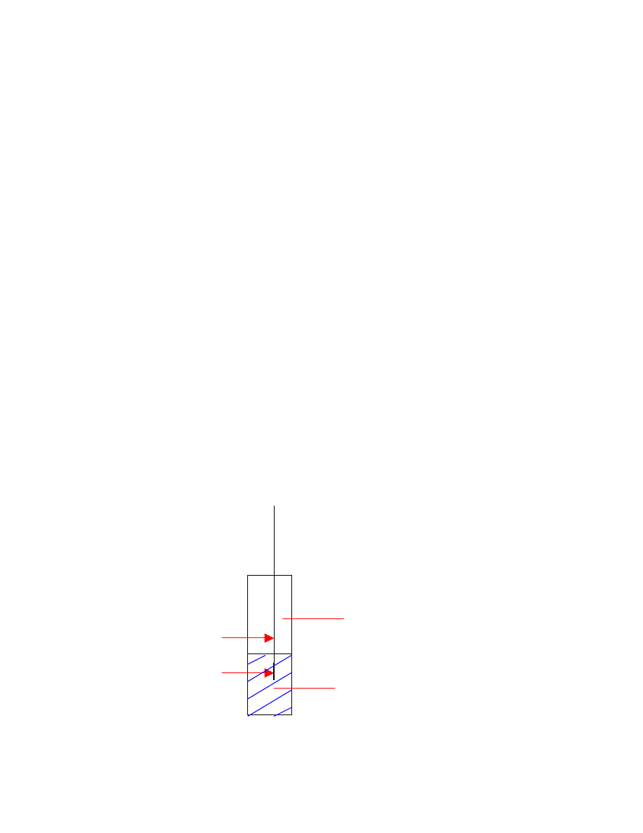
Let’s consider the following three phases, shown in Fig. 2.4 (direct sampling
mode), and Fig. 2.5 (headspace sampling mode):
•
fiber coating (f), with volume V
f
;
•
gas phase, or headspace (h), with volume V
h
;
•
homogeneous matrix (e.g. pure water) (s), with volume V
s
.
sample matrix
headspace (gas phase)
septum piercing
needle
fiber
Fig. 2.4: Direct sampling
17
Determination of coating volume:
A fused silica solid fiber is coated with a thin film of sorbent. The coating having a
cylindrical shape, its volume can be calculated using the formula for a cylindrical
section. Therefore, the volume of the fiber is:
(
)
h
r
R
V
2
2
f
−
π
=
where: R = radius of coated fiber
r = radius of uncoated fiber
h = length of the fiber
coating
thickness
=
R – r
Example: A carboxen/PDMS fiber, which has an 85
µ
m thick and 1 cm long coating,
on a fused silica rod of 110
µ
m internal diameter, would lead to a 0.5
µ
L volume for
the sorbent phase.
As long as the three volumes (fiber coating, headspace, and homogeneous matrix
volumes) are constant, the amount of analyte extracted is independent of the location of
the fiber in the system (headspace or directly in the sample) at equilibrium [35,36].
Fig. 2.5: Headspace sampling
headspace (gas phase)
sample matrix
fiber
septum piercing
needle

18
If we assume there are no losses (i.e., biodegradation or adsorption on walls of
sampling vessel), then mass is conserved, therefore the number of moles is conserved,
and the following equation can be written [35]:
s
s
h
h
f
f
s
0
V
C
V
C
V
C
V
C
∞
∞
∞
+
+
=
(1)
where:
•
C
0
is the initial concentration of the analyte in the matrix;
•
C
f
∞
, C
h
∞
, and C
s
∞
are the equilibrium concentrations of analyte in the fiber,
headspace, and solution (matrix) respectively.
The mass of analyte sorbed by the coating at equilibrium is:
f
f
V
C
n
∞
∞
=
(2)
Multiplying and dividing the right side of Eq. (2) by C
0
Vs, we obtain:
s
s
f
f
V
C
V
C
V
C
n
0
0
∞
∞
=
(3)
Replacing the denominator with the right term of Eq. (1), we get:
s
s
h
h
f
f
s
f
f
V
C
V
C
V
C
V
C
V
C
n
∞
∞
∞
∞
∞
+
+
=
0
(4)
Dividing both the numerator and denominator by
∞
s
C , we obtain:
s
s
h
h
s
f
f
s
s
f
f
V
C
V
C
C
V
C
C
V
C
V
C
n
+
+
=
∞
∞
∞
∞
∞
∞
∞
0
(5)
Let’s now define two partition coefficients that express the proportion of analyte at
equilibrium between two of the three phases:
1- Sample-coating partition coefficient:
∞
∞
=
s
f
spme
C
C
K
2- Sample-headspace partition coefficient:
∞
∞
=
s
h
hs
C
C
K
Note that a third partition coefficient (coating-headspace) could be defined, but it would
be dependent on the two previously defined partition coefficients.
Substituting these partition coefficients into Eq. (5), we get:

19
s
h
hs
f
spme
s
f
spme
V
V
K
V
K
V
C
V
K
n
+
+
=
∞
0
(6)
Let’s consider two cases: first the case where there is some headspace; second the case
where there is no headspace.
Case 1: There is headspace
Since V
f
is very small (
µ
L), generally K
spme
V
f
<< V
s
, Eq. (6) can be written as:
s
h
hs
s
f
spme
V
V
K
V
C
V
K
n
+
≅
∞
0
(7)
Dividing the numerator and denominator by V
s
, we get:
0
1
1
C
V
V
K
V
K
n
s
h
hs
f
spme
+
≅
∞
(8)
Note that the amount of analyte extracted at equilibrium by absorption is proportional
to C
0
and is dependent on the sample, headspace, and coating volumes.
Case 2: Assuming no headspace:
In the case there is no headspace ( V
h
= 0), Eq. (8) becomes:
0
C
V
K
n
f
spme
=
∞
(9)
This equation shows that the amount of analyte extracted (n) at equilibrium by
absorption, by direct sampling and in the absence of headspace, is independent of the
volume of the sample matrix (V
s
), and depends only on the initial analyte concentration
(C
0
) and coating volume (V
f
). This is very important, as it implies that it is not
necessary to sample a well defined volume of the matrix, which therefore allows easy
field sampling.
The same conclusions are valid for the adsorption process if the solution is dilute
enough.

20
2.3.2 Dynamic process (kinetics) of direct SPME
The amount of analyte extracted by the fiber, by direct sampling, is an increasing
function of time, as follows [2]:
]
1
[
/
s
t
e
n
n
τ
−
∞
−
=
(10)
where:
∞
n is the amount of analyte extracted at equilibrium, given by Eq. (9); and
τ
s
is
the time constant for direct sampling. This latter variable is a characteristic time of the
equilibrium process: the smaller the time constant the faster the equilibrium is achieved.
The time constant is dependent on mass transfer coefficients of the analyte in the
sample matrix and the polymer film, on sample and fiber volumes, on fiber-coating
coefficient, and on the surface area of the fiber coating. This time constant is directly
related to the sampling time needed to get the desired recovery percent. As we can see
in Table 2.1, extraction times higher than three time constants yield recovery percents
of at least 95%.
Table 2.1: Recovery percents for different sampling times
t
Recovery %
τ
s
63.2
2
τ
s
86.5
3
τ
s
95.0
4
τ
s
98.2
5
τ
s
99.3
6
τ
s
99.8
When the extraction time t reaches infinity (equilibrium conditions), the exponential
term reaches zero, and the amount extracted is equal to the amount extracted at
equilibrium. When t is held constant, the amount extracted is proportional to the
amount extracted at equilibrium, and hence is proportional to the initial concentration
of the analyte in the sample matrix. Thus, in theory, it does not matter what sampling
time is used, as long as the same sampling time is used for a determined set of

21
experiments. In practice, however, if the sampling time is too short, then a small error
in time measurement would lead to a large error in analyte amount extracted (high
curve slope). Therefore, in practice, it is better to choose a sampling time close to the
equilibrium condition, where the slope of the extraction time curve would start
approaching zero.
2.3.3 Dynamic process (kinetics) of headspace SPME
Headspace sampling involves two mass transfers which determine the speed of
extraction of the analytes by the fiber:
•
the mass transfer at the condensed/ headspace interface
•
the mass transfer at the headspace/ polymer interface
Case 1: Mass transfers are equal (steady state mass transfer)
The amount of analyte extracted as a function of time can be expressed as [2]:
]
1
[
/
h
t
e
n
n
τ
−
∞
−
=
(11)
Like previously,
∞
n is the amount of analyte extracted at equilibrium as given by Eq.
(8), and
τ
h
is the time constant for the headspace sampling mode. The time constant
now also depends on the evaporation constant of the solution. The same conclusions
can be reached as for the direct sampling mode.
Case 2: Mass transfers are not equal (non-steady-state mass transfer)
The amount of analyte extracted as a function of time can be expressed as the sum
of two exponential terms [2]:
]
1
[
]
1
[
2
1
/
/
τ
τ
β
α
t
t
e
e
n
−
−
−
+
−
=
(12)
The time constant
τ
2
depends only on the analyte diffusion rate in the polymer film.
The time constant
τ
1
depends on both the analyte evaporation into the headspace and
the analyte diffusion into the polymer phase. The coefficients
α
and
β
are both

22
proportional to C
0
, thus the analyte amount extracted is proportional to the initial
concentration of analyte in the solution, as long as the extraction time is held constant.
Hence, the same conclusion about the selection of a sampling time is achieved here.
2.4 Fibers
Since the fiber (coating) is the “heart” of the extraction, it is very important to
select the right fiber for the desired application. The fiber coating should be selected
based on film thickness and polarity [64].
The film thickness affects both speed and capacity. As film thickness increases,
film capacity is increased and speed is decreased. A film that is too thick may induce
carry-over of analytes from one sample to another. In today’s world, most of the time,
the fastest extraction would be wanted, meaning that the preferred choice for a fiber
would be one with a thin film. However, using a fiber with a thin film would not be
good if the fiber is not selective enough for the analytes of interest, and/or if the fiber
has a higher selectivity for other analytes (of non-interest). Therefore, in order to
determine what film capacity is wanted, we need to also take into account the amount
of analytes of non-interest that may have a high affinity for the fiber. Hence, a thin film
is best for analytes which have a significant affinity for the fiber (high fiber-coating
partition coefficient), whereas a thicker film would be preferred for other analytes.
The polarity of the fiber influences its selectivity according to the principle of
“like prefers like”: polar analytes are better extracted with a polar fiber, whereas non
polar analytes are better extracted with a non polar fiber.
Different coatings are available commercially in different thicknesses and
polarities, and the best combination of these latter needs to be determined according to
the coatings available on the market. The presently available coatings are either liquid
phases or porous particle blends. Supelco (State College, PA) has exclusive patent
rights for the sale of SPME fibers.

23
Liquid phases extract analytes by absorption, which is a non-competitive process.
Therefore the matrix composition does not affect the amount of analytes extracted, and
the linear range is broad [19]. These phases include Polydimethylsiloxane (PDMS),
Polyacrylate (PA), and Carbowax (CW). The PDMS phase is the first and most widely
used fiber. The PDMS phases are non polar and are the most commonly used due to
their versatility and durability. They are available in three film thicknesses: 100, 30,
and 7
µ
m. The PA phase is polar. At room temperature, it is not a liquid but a solid or
“glass” phase. The diffusion of the analytes in and out of the coating is slower, hence
the equilibration times are longer and the desorption temperature needs to be higher.
The CW phase is polar and water soluble. In order to reduce its water solubility it must
be crosslinked.
Porous particle blends extract analytes by adsorption, which is a competitive
process. Since there are a limited number of sites where analytes can bind to, analytes
of lower affinity for the coating can be displaced by analytes of higher affinity for the
coating. Therefore it is important to work at low analyte concentrations. The porous
particle blends have different pore sizes, and extract analytes based on their size. These
particle blends can be placed into three categories: micro-pores (< 20 A), meso-pores
(20-500 A), and macro-pores (>500 A). The carboxen coating consists of mostly micro-
pores, the divinylbenzene one consists mostly of meso-pores, and the templated resin
one consists mostly of macro-pores.
Stability of fiber coating:
If a fiber is improperly used, its coating may get stripped off, resulting in an
inefficient fiber with no more ability to extract analytes. The stability of the fiber
coating is determined by its physical attachment to the fused silica core [64]. Less
stable coatings can swell and dissolve in the presence of polar solvents or high
temperatures. Nonbonded coatings have no crosslinking agents and are therefore the
least stable. Crosslinked coatings have crosslinking agents (such as vinyl groups) which
interact with each other to form a more stable film, however they are not bonded to the
fused silica core. Finally, bonded coatings are the most stable because they not only

24
have crosslinking agents which interact with each other but they also are bonded to the
fused silica core (silanol bonds).
25
CHAPTER 3 - EXPERIMENTAL SETUP AND METHODS
3.1 Instrumentation
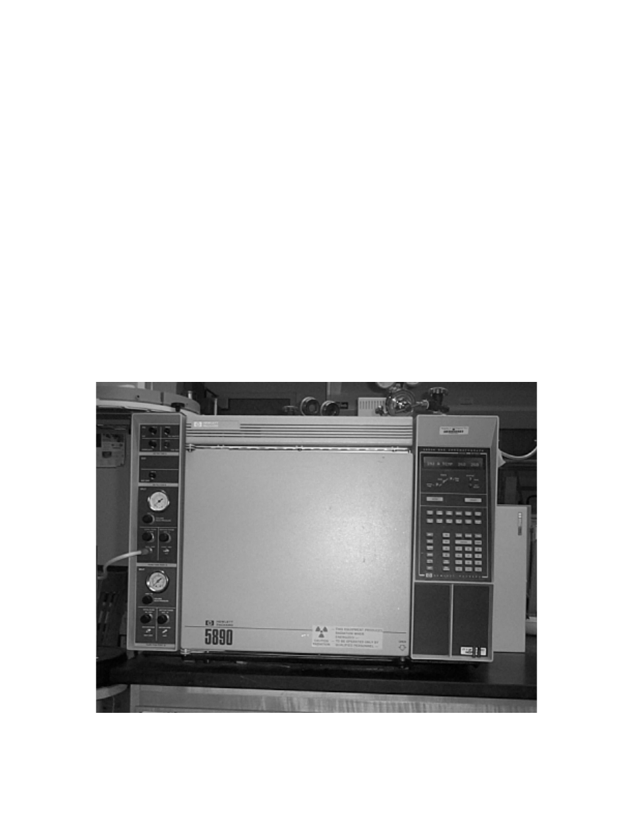
For the analysis and quantification of alcohols, we used a Hewlett Packard Model
5890 gas chromatograph, equipped with a flame ionization detector (FID) (shown in
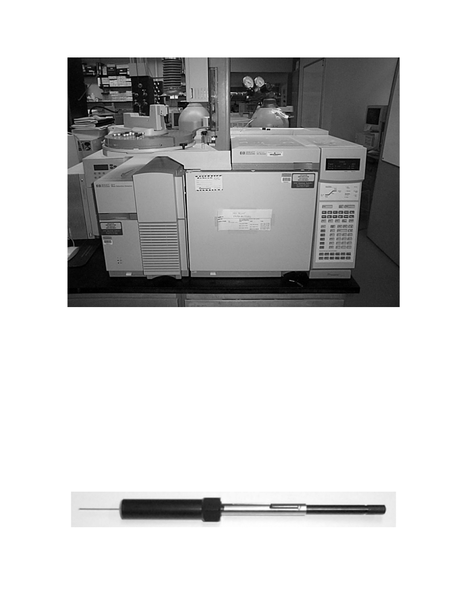
Fig. 3.1). In order to confirm peak identities, we used a HP Model 6890 gas
chromatograph, equipped with a mass selective detector HP Model 5973 (illustrated in
Fig. 3.2). Finally, for the sample preparation by SPME, we used a Supelco
fiberholder (shown in Fig. 3.3).
Fig. 3.1: HP-5890 GC
26
In the remainder of this chapter, we describe in detail the sample preparation steps
(Section 2), the GC analysis conditions (Section 3), and the data analysis techniques
that were employed (Section 4). Finally, Section 5 concludes the chapter with some
remarks on salt addition.
Fig. 3.2: GC-MS 5973, HP-6890
Fig. 3.3: Fiberholder

27
3.2 Sample preparation
3.2.1 Gasoline samples
Gasoline samples were obtained from a local gas station. In this area, oxygenates
are not required to be added since this is not a high pollution area. Indeed, due to
current gasoline and oxygenates prices, adding these to the gasoline would increase the
cost of making gasoline. Premium fuels may contain MTBE to increase the octane
number. Only regular unleaded gasoline samples will be used for this quantification
study, focused on the quantification of ethanol. Since the gasoline samples do not
contain any ethanol, we will make our own sample, containing 6.6 weight % EtOH (5.8
volume % EtOH), which corresponds to the 2 weight % oxygen required by the Clean
Air Act Amendments. The volume % of EtOH and MTBE required to obtain 2 weight
% and 2.7 weight % oxygen containing gasolines are given in Table 3.1. Densities of
ethanol and gasoline are given in Table 3.2, where the density of gasoline has been
determined by weighing a specific volume of gasoline. All the calculations used to
convert volume % oxygenates to weight % oxygenates are shown in detail in Appendix
A. We used anhydrous EtOH to prepare our “oxygenated” gasoline sample. We
assumed that the molecular interactions between any two mixing compounds are
negligible, which means that we consider the volumes additive (i.e., the total volume is
equal to the sum of the individual volumes). We also assumed that the temperature
change across experiments is negligible.
Table 3.1: Relation between oxygenate amounts and volumes
Oxygenate
Wt. % Oxygen
Vol. % Oxygenate
2.0 5.8
EtOH
2.7 7.8
2.0 11
MTBE
2.7 14.8

28
3.2.2 Mixing procedure
As mentioned in Chapter 1, it can be difficult to quantify oxygenates in gasoline
by simple gas chromatography, due to hydrocarbon interferences with the oxygenated
additives. As can be seen in Table 3.3, gasoline is composed of about 48.9 % aliphatics
and 48.6 % aromatics, with about 94.5 % of the aromatics and only 1.3 % of the
aliphatics being water soluble. Therefore, most of the aliphatic compounds (and also
some aromatic compounds) can be left behind by extracting them with water. This is
the approach that will be used here. It is similar to the one used by Pauls and McCoy
[34], who used a water extraction step before a GC analysis. Their method has the
problem of introducing water into the GC, which is detrimental for the selected column.
In this section we will describe the procedure of extraction and how to obtain the
diluted solution that will be analyzed by SPME-GC.
Table 3.3: Regular unleaded gasoline water solubility
% wt.
% wt.
Alkanes(enes) Aromatics
Neat
Gasoline
48.9% 48.6%
Water
Soluble
Fraction
1.3% 94.5%
Table 3.2: Densities at 25
°°°°
C
Compound Density
(g/mL)
EtOH 0.7760
gasoline 0.6752

29
The mixing procedure consists of five steps:
1- Mix 2 mL of gasoline with 2 mL of HPLC grade water
2- Shake well for 1 minute
3- Wait 4 minutes, until phase separation occurs
4- Discard the (top) gasoline layer
5-
Take
10
µ
L of aqueous layer and dilute to 100 mL with HPLC grade water
An original 6.6% EtOH solution would be diluted to 6.6 ppm using that procedure.
3.2.3 SPME conditions
The following conditions have been used:
•
Fiber: Carboxen-PDMS
•
Sampling type: Direct sampling in water
•
Extraction time: 10 minutes with stirring
•
Desorption time: 10 minutes at 260
°
C
Several fibers have been evaluated, however this was the fiber of choice since this
was the one showing the least amount of interfering peaks. This also is the most polar
fiber commercially available. Carboxen is a carbon molecular sieve, consisting of solid
particles (2 to 10
µ
m thick) embedded in a PDMS phase. Its small pores allow
separation of small analytes by retention in the pores. This is another interesting feature
of this fiber since the alcohols of interest are relatively small (MeOH and EtOH
molecular weights are 32 and 46 Daltons respectively).
Both direct and headspace sampling were considered. However, direct sampling is
preferred due to better sensitivity.
The extraction time, t, has to satisfy the following equation, derived in Appendix
B:
+
∆
≥
1
ln
ετ
τ
t
t
where:
∆
t is the error in extraction time measurement;
τ
is the time constant of the
extraction process; and
ε
is the maximum relative error in analyte amount extracted.

30
An extraction time of 10 minutes for direct sampling satisfies this equation and therefore
was chosen for direct sampling. The next Chapter details an extraction time study in both
direct and headspace sampling.
A desorption time of 10 minutes was experimentally chosen since it is long
enough to avoid carry-over from one sample to another.
3.3 GC conditions
The following GC conditions were used:
•
Column: HP-INNOWAX (crosslinked polyethylene glycol), 30 m long, with 1.0
µ
m
film thickness and 0.53 mm i.d. This is a polar column.
•
Oven temperature program: 65
°
C for 4 min; program to 200
°
C at 60
°
C/min
•
Injector temperature: 260
°
C
•
Detector (FID) temperature: 290
°
C
•
Operating mode: splitless, with purge valve open after 1 min
•
Column headpressure: 2 psi, linear gas velocity: 41 cm/sec
Both MeOH and EtOH are polar and have relatively low boiling points (64.6
°
C
and 78.3
o
C respectively). Therefore, a non polar column (such as DB-5) allows a fast
analysis; however, it does not allow good resolution because of the alcohols’ close
boiling points. A polar column (such as HP-INNOWAX) will solve this problem, by
allowing a higher retention of the alcohols in the column stationary phase. We used a
HP-INNOWAX column, with a 30 meter length, a 1.0
µ
m film thickness, and a 0.53
mm internal diameter. A “fat” film, as well as a big internal diameter has been chosen,
in order to obtain an even greater retention of the alcohols and therefore yield a better
separation.
We initially used the following oven temperature program (later changed to the
current temperature program). We started the oven temperature at 40
°
C, held it for 3
minutes, then ramped the temperature up to 60
°
C at 10
°
C/min in order to separate the

31
two alcohols. Finally, we ramped the temperature up to 200
°
C at 40
°
C/min and held it
at 200
°
C for 10 minutes, in order to eliminate all the remaining gasoline components.
This oven temperature program allowed good separation of methanol and ethanol.
However, an unknown compound (which was later identified as benzene by GC-MS)
was found to be interfering with the ethanol. In order to solve this interference problem
and be able to quantify EtOH, we changed the temperature program to the following
one. The temperature is first held constant at 65
°
C for 4 minutes in order to allow a
good separation of methanol and benzene. Then it is rapidly increased to 200
°
C at a
rate of 60
°
C/min and held at 200
°
C for 10 min, in order to eliminate the remaining
gasoline compounds. Note that a rate of 60
°
C/min will probably not be achieved,
however this programming ensures that the remaining compounds will be eliminated as
fast as possible. Moreover, our experimental results will not be affected by the actual
rate. We now focus solely on the EtOH and ignore the MeOH. This is feasible since our
original gasoline sample does not contain MeOH.
The injector temperature is set at 260
°
C, which is also the fiber desorption
temperature. The detector used is a flame ionization detector (FID), set at 290
°
C.
The operating mode is splitless, with the purge valve open after 1 minute. A
SPME liner (0.75 mm internal diameter) is used instead of the conventional splitless
liner (2 mm internal diameter), in order to allow a faster flow rate through the liner.
This allows the analytes to be more focused at the beginning of the column, therefore
resulting in narrower chromatographic peaks.
Finally, the column headpressure is set at 2 psi, in order to have a flow rate
through the column of 5.4 mL/min, corresponding to an average linear velocity of 41
cm/sec.
3.4 Data analysis
Two data analysis approaches are considered: the method of calibration curve
(using calibration standards), and the method of standard addition.

32
3.4.1 Method of calibration curve
In the method of calibration curve, standard solutions with different alcohol
concentrations are prepared in water. A calibration curve is then constructed, by
plotting the detector responses (peak areas) versus the alcohol concentration. The linear
portion of that curve will be used to find the alcohol concentration in an unknown
sample. This method works well if the standard solutions are prepared in the same
matrix as the actual samples. However, it may not be accurate in our case. Since the
SPME of alcohols in gasoline from water is done in a slightly different matrix than the
extraction of pure alcohols from water, the calibration curve may vary slightly.
Moreover, there is the possibility of errors due to non-quantitative transfer in the
mixing procedure. The method of calibration curve should be preferred whenever non-
oxygenated gasoline of the same type of the one to be analyzed is available. Indeed,
once the calibration curve is plotted, it can be used to analyze several gasoline samples.
Only one measurement or one set of replicates is needed to quantify the ethanol amount
in a desired gasoline sample. Therefore this method would be fast and very useful for
quality control measurements.
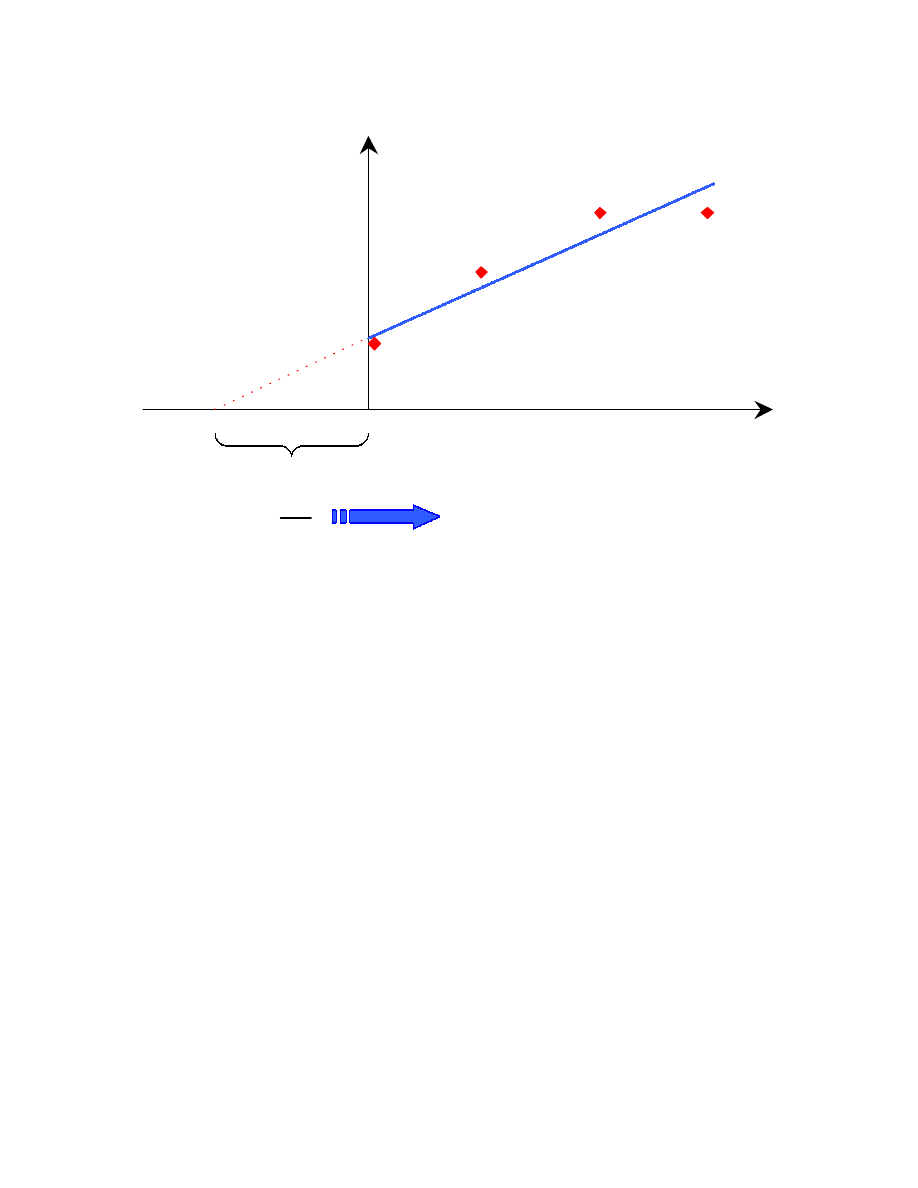
3.4.2 Method of standard addition
The method of standard addition consists in spiking different amounts of alcohols
in the oxygenated gasoline sample in order to obtain solutions with different alcohol
concentrations. The detector response can then be plotted against the added
concentration of alcohol. This is referred to as a standard addition curve (Fig. 3.4). The
unknown EtOH concentration can be found by extrapolating the best fit line to the x-
axis intercept. That intercept will be the unknown EtOH concentration. If the equation
of the best fit line is written in the form y = mx + q, then the x-axis intercept is equal to
the y-axis intercept (q) over the slope (m).
33
In this research, we spiked respectively 40, 80, 120, and 160
µ
L of EtOH in the
6.6 weight % EtOH gasoline solution, in order to get gasoline solutions of respectively
8.7, 10.7, 12.6, and 14.4 weight % EtOH. These solutions were then further extracted
with water and diluted to the desired ppm amounts for analysis. The details of these
computations are explained in Appendix A. This method is a little more time
consuming than the previous one, since each gasoline sample analysis requires 4 to 6
measurements (original sample and spiked samples) or 4 to 6 sets of measurements.
Therefore it would be good to use by the regulatory agencies, since these would be
interested in analyzing gasoline samples of various composition. In the quality control
case, however, where the gasoline samples contain the same amounts of different
components, this method does not offer any major advantage over the first one, but is
q
m x
y
+
=
A
rea C
o
u
n
ts
Added EtOH (ppm)
m
q
Unknown EtOH
concentration
Fig. 3.4: Standard addition method
Unknown EtOH
concentration

34
more time consuming. Therefore, in this case, the first method would be the preferred
one.
3.5 Salt addition
It is common, in some SPME applications, to add salt to an aqueous solution in
order to reduce the solution’s solvating power [36,48,64]. Hence, moderately water
soluble compounds may be “salted out” and go into the headspace and/or the SPME
fiber. In this case, adding salt to the solution has been tried and discarded. The salt,
after a few samplings, can get onto the fiber and is difficult to be remo ved. Also there is
an accumulation of salt in the liner, which implies that the liner needs to be taken out of
the GC and cleaned often.

35
CHAPTER 4 - RESULTS AND DISCUSSION
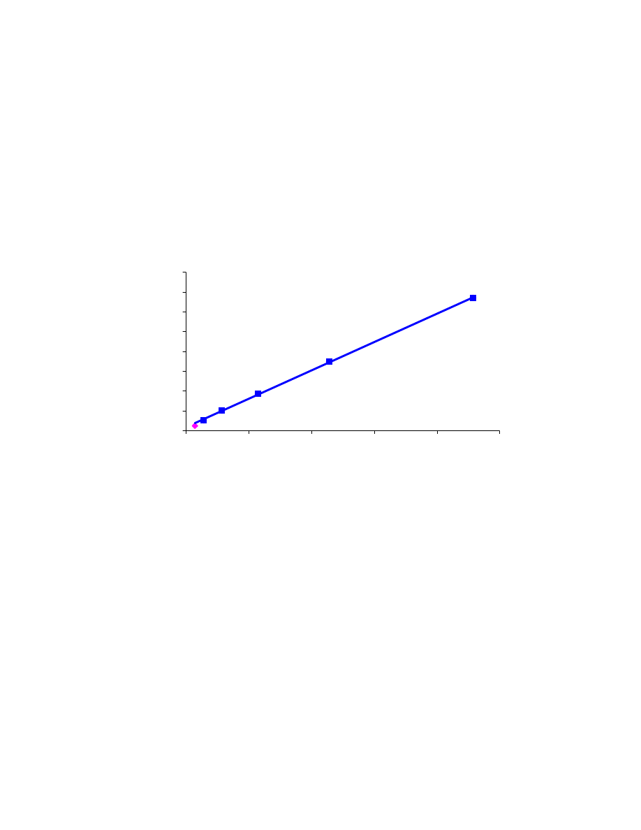
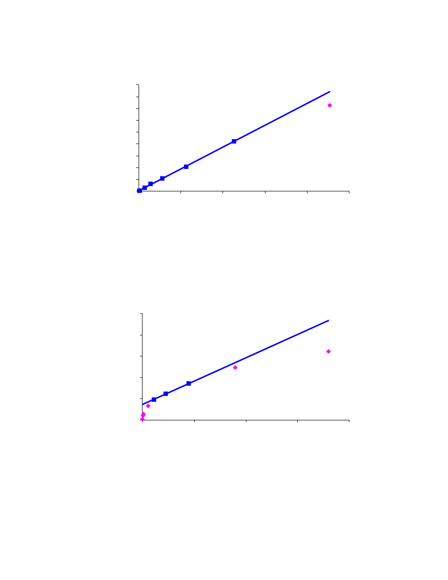
4.1 Linearity curves
In order to verify the linear range of quantitative GC methods for methanol,
ethanol, and methyl-tert-butyl-ether in water, linearity curves were experimentally
determined and are shown in Figs. 4.1, 4.2 and 4.3 respectively. In these curves the blue
points exhibit a close to linear behavior and therefore are used to fit the linear model,
obtaining a very good R
2
value. On the contrary, the pink points indicate measurements
significantly departing from linearity. The linearity ranges for the two alcohols and the
ether were found to be much larger than what has been reported in the literature [41].
Indeed, using the carboxen/PDMS fiber for the analysis of C
1
-C
8
alcohols and MTBE
in water, linear ranges of respectively 10 ppb to 1 ppm and 1 ppb to 500 ppb were
reported [41]. In this study we found the methanol curve to be linear between 14 and
229 ppm, the ethanol curve to be linear between 0.7 and 113 ppm, and the MTBE curve
to be linear between 10 and 45 ppm. The two lowest MTBE concentrations we used
were 40 ppb and 390 ppb; lower MTBE concentrations would need to be prepared and
analyzed quantitatively in order to check for linearity at lower MTBE levels.
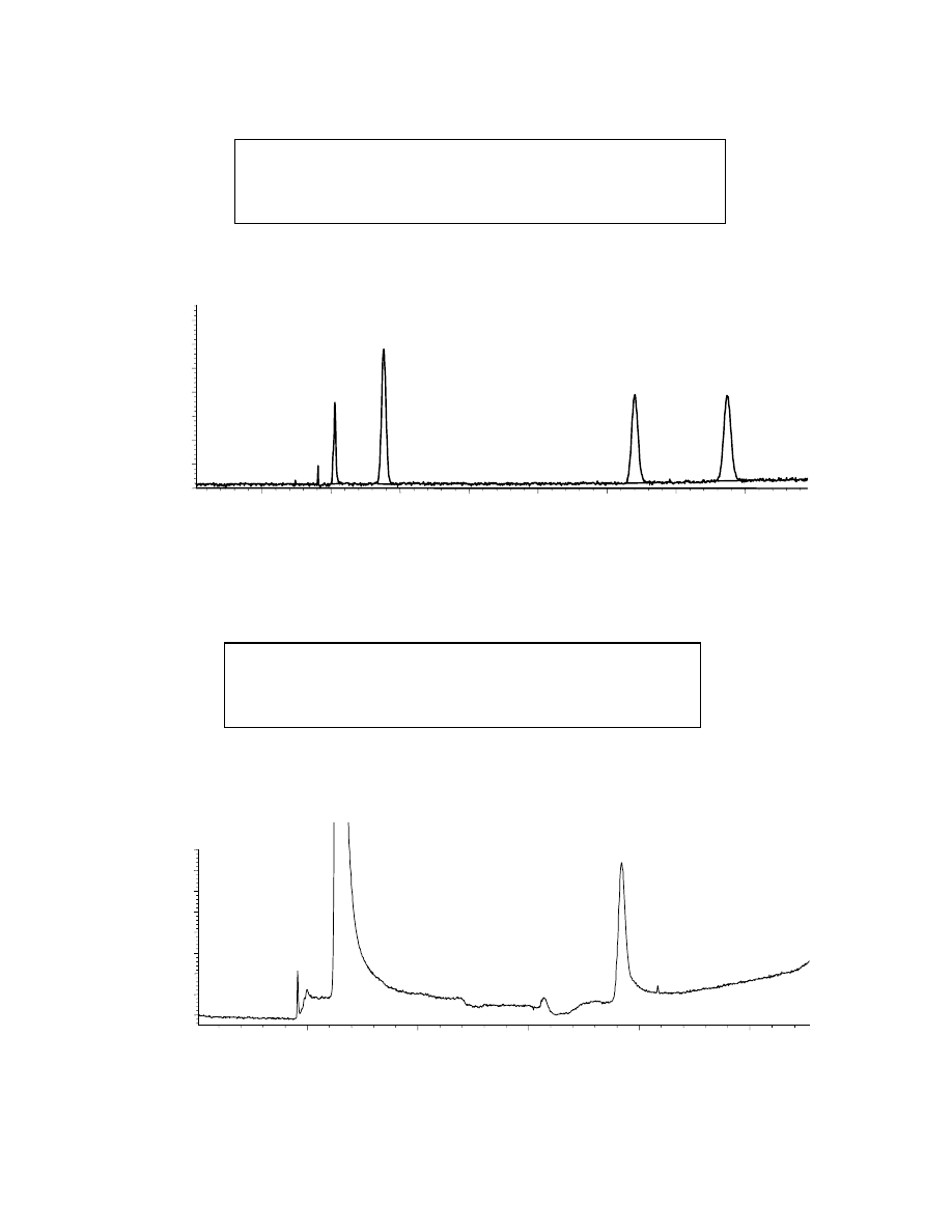
A simple GC injection of 2900 ppm MeOH, 2500 ppm EtOH and 1800 ppm
MTBE in water, through a 4 mm i.d. splitless liner, was performed for peak area
reference. The corresponding chromatogram (Fig. 4.4) showed very similar peak areas
for the three analytes. A SPME-GC experiment was then performed using a solution of
oxygenates in water that is 400 times more dilute than the one used for simple GC
injection (in order not to saturate the fiber). The corresponding chromatogram (Fig. 4.5)
showed significantly different peak areas for each of these oxygenates even though they
were spiked into water at similar concentrations. The polar fiber is more selective for
MTBE than for the alcohols. Indeed, MTBE is the least polar of these compounds,
therefore it likes the water the least and has the highest sample-coating partition
coefficient. Methanol, which is the most polar of these three oxygenates, likes to stay in
36
the water the most and therefore has the lowest sample-coating partition coefficient.
Ethanol, which is more polar than MTBE, and slightly less polar than MeOH, has an
intermediate partition coefficient, and therefore an intermediate peak area.
y = 28.7 x + 172.8
R
2
= 0.9996
0
1000
2000
3000
4000
5000
6000
7000
8000
0
50
100
150
200
250
Concentration (ppm)
Area Counts
Fig. 4.1: Linearity curve for methanol (F.I.D)
37
y = 369.6 x + 261.5
R
2
= 0.9991
0
10000
20000
30000
40000
50000
60000
70000
80000
90000
0
50
100
150
200
250
Concentration (ppm)
Area Counts
Fig. 4.2: Linearity curve for ethanol (F.I.D)
y = 1097.6 x + 36274
R
2
= 0.9989
0
50000
100000
150000
200000
250000
0
50
100
150
200
Concentration (ppm)
Area Counts
Fig. 4.3: Linearity curve for methyl-tert-butyl-ether (F.I.D)
38
min
Fig. 4.4: GC of oxygenates spiked into water
EtOH
3.87
1
2
3
4
counts
-
1300
-
1200
-
1100
-
1000
MTBE
1.38
MeOH
3.20
Column: HP-INNOWAX, 30 m
×
0.53 mm i.d.
×
1.0
µ
m f.t.
Oven: 40
°
C (3 min) to 62
°
C (0 min) @ 10
°
C/min
to 200
°
C (10 min) @ 40
°
C/min
Fig. 4.5: SPME-GC of oxygenates spiked into water
EtOH
3.84
4
1100
MTBE
1.27
2
counts
1200
min
1
3
5
800
900
1000
MeOH
3.13
1300
1400
1500
Column: HP-INNOWAX, 30 m
×
0.53 mm i.d.
×
1.0
µ
m f.t.
Oven: 40
°
C (3 min) to 62
°
C (0 min) @ 10
°
C/min
to 200
°
C (10 min) @ 40
°
C/min
39
4.2 Extraction time curves
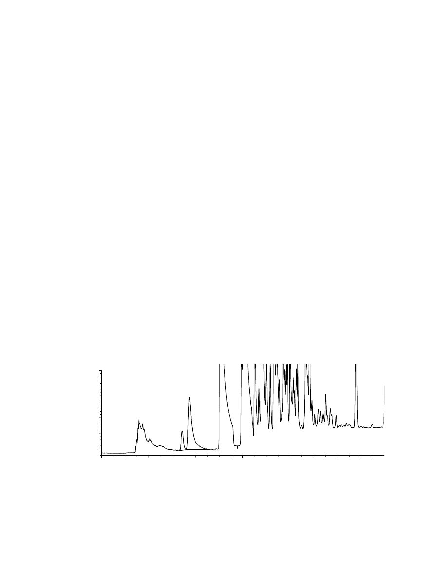
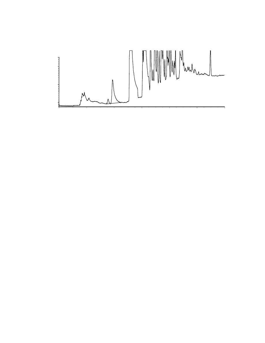
The water extraction procedure was shown to be effective in eliminating
interfering hydrocarbon peaks. Only the interfering benzene remains in the solution at
our limits of detection. Selecting the right oven temperature program, as described in
Chapter 3, allows us to obtain good separation of EtOH and benzene, as can be seen in
Figs. 4.6 and 4.7. The chromatogram in Fig. 4.6 has been obtained using a 39 ppm
EtOH in water solution, corresponding to a 5.7 weight % EtOH in the original gasoline
stock solution. The EtOH and benzene peaks are well separated, and therefore easily
quantifiable. In order to avoid fiber saturation, we decided to work with a more dilute
sample. We chose a 4.3 ppm EtOH in water diluted sample, corresponding to a 6.2
weight % EtOH in the gasoline stock solution. As seen in Fig. 4.7, EtOH was detected,
therefore our method is good for quantifying EtOH at these levels. Unfortunately, this
EtOH concentration does not fall in the linear range of quantification, therefore there
may be slight inaccuracies in the quantification of EtOH. However, a more dilute
Benzene
3.74
min
0
2
4
6
8
10
counts
-500
0
500
1000
1500
EtOH
3.43
Fig. 4.6: SPME-GC of 39 ppm EtOH in the water extracted gasoline fraction
40
solution could not be used since the EtOH peak would have been smaller than the limit
of quantification (LOQ).
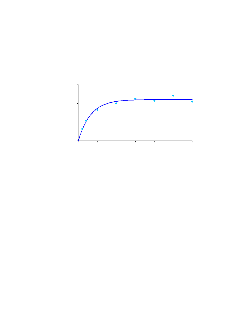
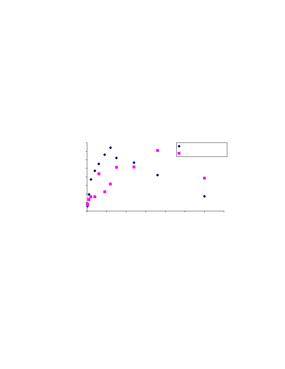
As a first step in the analysis, we performed an extraction time study, that is we
studied how the area counts for EtOH vary with different extraction times. Two
extraction time curves were plotted, one by performing direct sampling experiments
(Fig. 4.8), the other, by performing headspace sampling experiments (Fig. 4.9), both
using a 4.5 ppm EtOH in water dilute solution. These two extraction time curves only
show qualitative results, since the fiber used for the direct sampling study was stripped
off before the headspace sampling study could be done. A different fiber had to be
used, and therefore quantification was not possible.
As was shown in Chapter 2, it is not necessary to choose a sampling time close to
equilibrium, since at any time the amount of analyte extracted by the fiber is directly
proportional to the initial concentration of analyte in the solution. However, it is
important to choose an extraction time where the slope is low in order to minimize the
propagation of error, since a slight error in extraction time directly propagates into an
error in area counts. The steeper the slope, the higher the error in area counts for a
min
0
2
4
6
8
10
counts
-
600
-
400
-
200
0
200
EtOH
3.56
Benzene
3.88
Fig. 4.7: SPME-GC of 4.3 ppm EtOH in the water extracted gasoline fraction
41
given error in extraction time measurement. In the direct sampling case (Fig. 4.8), the
amount of analyte extracted increases relatively quickly during the first five minutes.
Then it levels out, until it is stable. In Appendix B, it is proven that, if the error in
sampling time measurement is 5 seconds, the sampling time has to be at least 4.2
minutes. Using a conservative approach we chose a sampling time of 10 minutes.
Using headspace sampling (Fig. 4.9), the amount of EtOH extracted increases
rapidly during the first 60 minutes. After 60 minutes, instead of increasing more slowly
and reaching a steady value, it starts decreasing. This phenomenon may be
characteristic of this carboxen/PDMS fiber, as it saturates with gasoline components.
Figure 4.9 also shows the amount of other compounds (divided by 200 in order to
properly scale the plot) extracted by the fiber during the same analysis. It can be
noticed that as the amount of EtOH extracted starts to decrease, the amount of other
compounds still increases, which seems to confirm the presence of displacement
effects. However, the last sampling point is an exception in that the amount of both
EtOH and other compounds extracted decreased. This is probably due to evaporative
losses in the sampling vial. The carboxen/PDMS fiber does not behave exactly like the
other adsorption type fibers, and no extraction theory is available for it yet [19]. Since
Fig. 4.8: Direct sampling extraction time curve
0
200
400
600
0
5
10
15
20
25
30
Extraction Time (min)
Area Counts
(
)
9685
.
0
1
440
2
3
.
3
/
=
−
=
−
R
e
A
t
42
the carboxen coating has such small pores, capillary condensation could occur, leading
to a greater adsorption capacity for some analytes [19]. This capillary condensation can
occur in addition to the possible replacement effects (where analytes with low affinity
for the fiber are displaced by analytes with higher affinity for the fiber) common to
adsorption type fibers. The capillary condensation effect is negligible if the analytes’
concentrations are low enough [19]. Thus, as long as the EtOH level stays above the
limit of quantification, it might be advisable to use a more dilute water extracted
gasoline solution. Also, using a more polar fiber (not yet commercially available) may
improve the method’s % RSD’s.
4.3 Standard addition curves
In this section, the method of standard addition is used to quantify the amount of
EtOH present in the stock solution. The stock solutions are first extracted with water
and then diluted with water to the corresponding ppm amount. The standard addition
curves are plotted using the added ppm amounts of the EtOH in the water fraction.
Fig. 4.9: Headspace sampling extraction time curve
0
500
1000
1500
2000
2500
3000
3500
4000
0
50
100
150
200
250
300
350
Extraction Time (min)
Area Counts
EtOH
Other compounds/200

43
Once the ppm amount of the EtOH in the water fraction is determined using the
standard addition curve, the weight % EtOH in the gasoline stock solution can be
calculated.
Three experimental sets using direct sampling will be presented:
1 - using a 5.7 % EtOH stock solution
2 - using a 6.6 % EtOH stock solution, prepared right before using it for obtaining
the diluted solutions
3 - using a 6.6 % EtOH stock solution, used to prepare the dilute solutions 24
hours after it was prepared
Each experiment comprises five solutions, the first being the original solution
(diluted from the stock solution) and the other four being spiked ones (diluted from the
spiked stock solution). For each solution, three replicate analyses were performed to
average out errors. The average, standard deviation and percent relative standard
deviation (% RSD) were calculated and plotted on a graph of area counts versus added
concentration of EtOH in water (in ppm). Other researchers have reported an average
value of 10 % RSD when using SPME in the same concentration levels as used in this
research, therefore a 10 % RSD will be considered as reasonable. Note that a standard
deviation is not very meaningful when only three samples are used, however it still
gives some indication about the results’ precision. It was more important for us to be
able to perform the entire study during the same day in order to avoid day-to-day
instrument and/or solutions variations; therefore more than three replicates for each
solution was not possible.
In the first set of results (Table 4.1), the %RSD values are reasonable, even
though two of them are slightly above 10%. The measurements, along with error bars
representing their standard deviation, are shown in Fig. 4.10. The R
2
value obtained for
the best fit line is slightly lower than 0.9, meaning that the line fits the results
reasonably well. The EtOH concentration in water is found to be 4.1 ppm, which
corresponds to a 6.0 weight % EtOH in gasoline. The actual weight % EtOH in gasoline
being 5.7 %, our results reflect a 5.3 % error with respect to the “true” EtOH
concentration in gasoline.
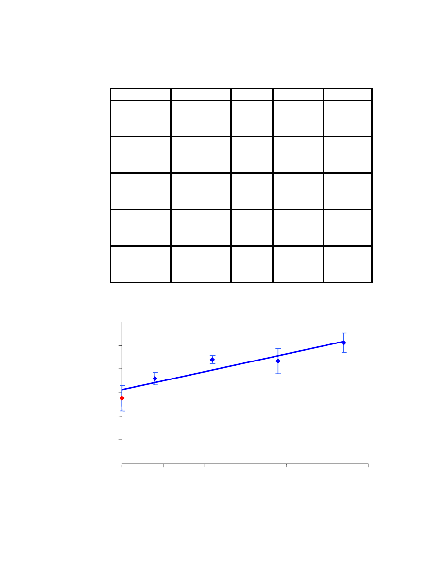
44
Table 4.1: Data set 1, using 5.7 wt.% EtOH stock solution
(3.9 ppm EtOH in water)
S olution
EtOH Ar e a Ave ra ge S td. De v.
%RS D
1
558.6
(original)
X
657.9
553.1
107.7
19.5
(3.9 ppm )
442.7
2
695.9
X + 0.4 ppm
681.1
718.7
52.8
7.3
(4.3 ppm )
779.0
3
899.5
X + 1.1 ppm
837.1
880.0
37.2
4.2
(5.0 ppm )
903.4
4
827.7
X + 1.9 ppm
986.9
866.4
106.5
12.3
(5.8 ppm )
784.7
5
962.7
X + 2.7 ppm
1081.9
1022.3
84.3
8.2
(6.6 ppm )
outlier
Fig. 4.10: Standard addition curve using result set #1
0
200
400
800
1000
1200
0
0.5
1
1.5
2
2.5
3
600
Added EtOH (ppm)
R
2
= 0.8717
Ar
ea Cou
n
ts
y = 151.7 x + 623.0
Unknown EtOH concentration in water: 4.1 ppm
Unknown EtOH concentration in gasoline:
6.0 wt.%
(5.3 % error)
5.7 wt. % EtOH stock solution

45
The second set of results is presented in Table 4.2. All five solutions show a
percent RSD less than 5.5 %. The measurements are shown in Fig. 4.11. The line fits
the results very well (R
2
= 0.9915). The EtOH concentration in water is found to be 4.1
ppm, which corresponds to a 6.0 weight % EtOH in gasoline stock solution. The actual
weight % EtOH in gasoline being 6.6 %, our results reflect a 9.1 % error with respect to
the “true” EtOH concentration in gasoline.
Table 4.2: Data set 2, using 6.6 wt.% EtOH stock solution (time 0)
(4.5 ppm EtOH in water)
Solution
EtOH Ar e a
Ave ra ge Std. De v.
%RS D
A
352.1
(original)
X
363.0
366.8
16.9
4.6
(4.5 ppm)
385.2
B
489.4
X + 1.6 pp m
441.3
469.6
25.2
5.4
(6.1 ppm)
478.1
C
577.4
X + 3.1 pp m
562.6
578.9
17.1
3.0
(7.6 ppm)
596.7
D
706.4
X + 4.7 pp m
749.6
742.7
33.4
4.5
(9.2 ppm)
772.1
E
888.5
X + 6.2 pp m
890.9
878.9
18.8
2.1
(10.7 ppm)
857.3
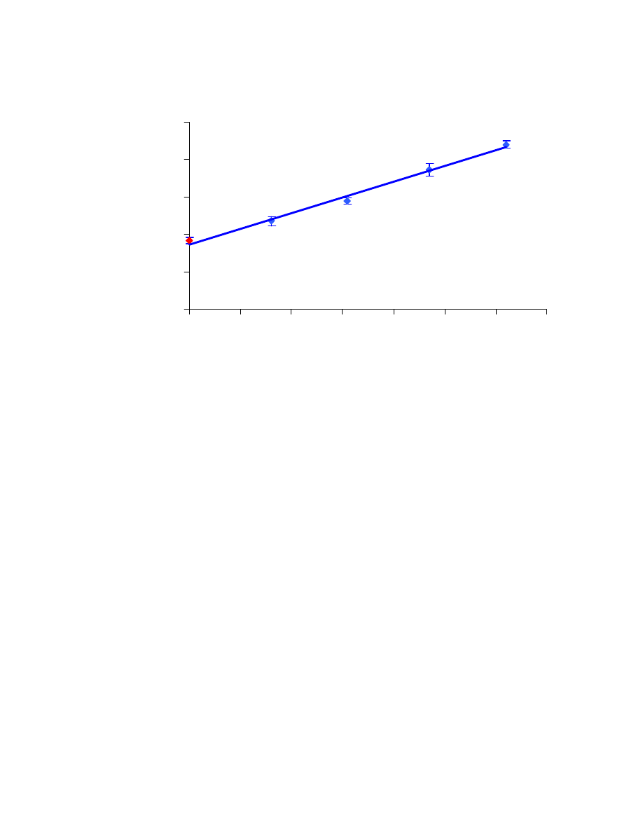
46
The third set of results is presented in Table 4.3. Most of the solutions show a
percent RSD below 6.1 %, with only one of them having a % RSD above 10 %. The
measurements are shown in Fig. 4.12. The graph shows a line that fits the results very
well (R
2
= 0.9910). The EtOH concentration in water is found to be 5.1 ppm, which
corresponds to a 7.5 weight % EtOH in gasoline stock solution, yielding a 14 % error in
the measurement of EtOH content in gasoline.
Fig. 4.11: Standard addition curve using result set #2
y = 83.7 x + 346.3
R
2
= 0.9915
0
200
400
600
800
1000
0
1
2
3
4
5
6
7
Added EtOH (ppm)
Area Counts
Unknown EtOH concentration in water: 4.1 ppm
Unknown EtOH concentration in gasoline:
6.0 wt.%
(9.1 % error)
6.6 wt. % EtOH stock solution
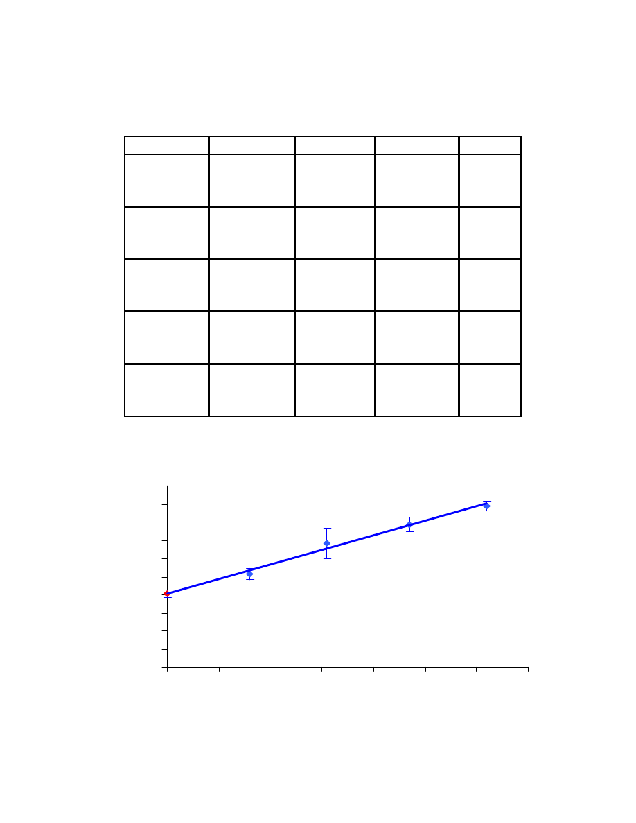
47
Table 4.3: Data set 3, using 6.6 wt.% EtOH stock solution (time 48 hours)
(4.5 ppm EtOH in water)
Solution
EtOH Ar e a
Ave ra ge
Std. De v.
%RSD
A
384.4
(original)
X
421.3
405.7
19.1
4.7
(4.5 ppm)
411.4
B
502.2
X + 1.6 ppm
487.8
512.6
31.4
6.1
(6.1 ppm)
547.8
C
769.5
X + 3.1 ppm
671.0
681.6
83.1
12.2
(7.6 ppm)
604.3
D
742.1
X + 4.7 ppm
812.0
785.9
38.2
4.9
(9.2 ppm)
803.5
E
865.5
X + 6.2 ppm
916.9
889.3
25.9
2.9
(10.7 ppm)
885.4
y = 80.0 x + 405.4
R
2
= 0.9910
0
100
200
300
400
500
600
700
800
900
1000
0
1
2
3
4
5
6
7
Adde d EtO H ( ppm )
Area Counts
6.6 w t. % EtO H stock solution
Fig. 4.12: Standard addition curve using result set #3
Unknown EtOH concentration in water: 5.1 ppm
Unknown EtOH concentration in
gasoline:
7.5 wt.%
(14 % error)
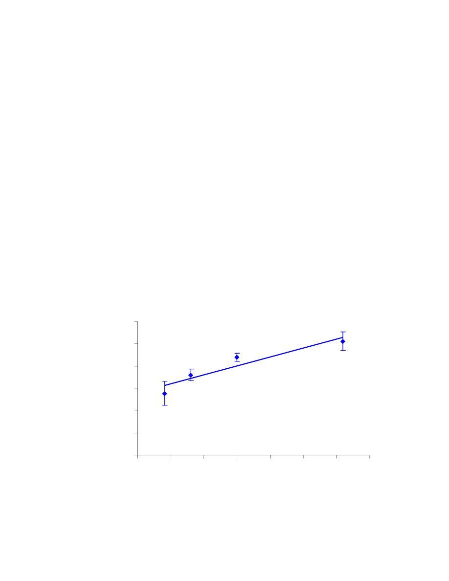
48
4.4 Calibration curves
In this section calibration curves are used to quantify the amount of EtOH present
in the stock solution. Since the gasoline samples obtained from a local gas station do
not contain alcohols, it is possible to use this method. Standard solutions with known
amounts of EtOH were prepared. Stock solutions with known amounts of EtOH can
then be anlyzed to test the accuracy of this method. In this work, for practical purposes,
we used the solutions that were prepared for the standard addition method. We selected
four solutions to be our calibration standards. The remaining solution was considered as
our unknown sample. Three results are presented, one each taken from the three data
sets previously described (Section 4.4).
From the first data set, we chose solution 4 (8.3 weight % EtOH in gasoline) to be
our unknown sample, with solutions 1,2,3 and 5 acting as the calibration standards. The
calibration curve hence obtained is shown in Fig. 4.13. The R
2
value of the best fit line
Fig. 4.13: Calibration curve using result set #1
y = 160.7 x - 1.8
R
2
= 0.8905
0
200
400
600
800
1000
1200
3.5
4
4.5
5
5.5
6
6.5
7
EtOH Concentration (ppm)
Ar
ea Cou
n
ts
Unknown EtOH concentration in water: 5.4 ppm
Unknown EtOH concentration in gasoline:
7.7 wt.%
(7.2 % error)
8.3 wt. % EtOH stock solution
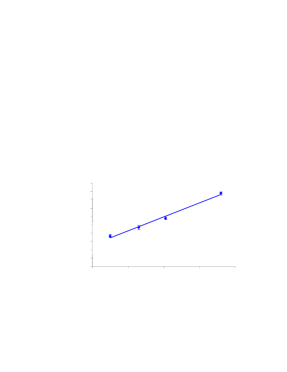
49
is slightly lower than 0.9, which is acceptable. The unknown EtOH concentration in
water is found to be 5.4 ppm, which corresponds to 9.5 weight % EtOH in gasoline.
This results in a 7.2 error %.
From the second data set, we chose solution D (12.6 weight % EtOH in gasoline)
to be our unknown sample, with solutions A,B,C, and E acting as the calibration
standards. The calibration curve is illustrated in Fig. 4.14. The R
2
value is 0.9902,
which means the best fit line fits the data very well. The unknown EtOH concentration
in water is found to be 9.3 ppm, which corresponds to 12.8 weight % EtOH in gasoline.
This results in a 1.6 error %.
y = 83.4 x - 28.9
R
2
= 0.9902
0
100
200
300
400
500
600
700
800
900
1000
3.5
5.5
7.5
9.5
11.5
EtOH Concentration (ppm)
Ar
ea Cou
n
ts
Unknown EtOH concentration in water: 9.3 ppm
Unknown EtOH concentration in gasoline:
12.8 wt.%
(1.6% error)
12.6 wt. % EtOH stock solution
Fig. 4.14: Calibration curve using result set #2
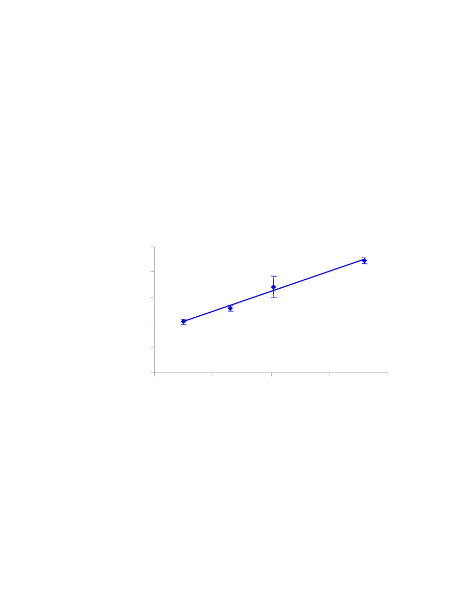
50
From the third data set, we chose solution D (12.6 weight % EtOH in gasoline) to
be our unknown sample, with solutions A,B,C, and E acting as the calibration
standards. The calibration curve is illustrated in Fig. 4.15. The R
2
value is 0.9898,
which means the line fits the data very well. The unknown EtOH concentration in water
is found to be 9.3 ppm, which corresponds to 12.8 weight % EtOH in gasoline. This
results in a 1.6 error %.
y = 79.6 x + 47.4
R
2
= 0.9898
0
200
400
600
800
1000
3.5
5.5
7.5
9.5
11.5
EtOH Concentration (ppm)
Ar
ea Cou
n
ts
Unknown EtOH concentration in water: 9.3 ppm
Unknown EtOH concentration in gasoline:
12.8 wt.%
(1.6 % error)
12.6 wt. % EtOH stock solution
Fig. 4.15: Calibration curve using result set #3

51
CHAPTER 5 - CONCLUSIONS
The Clean Air Act Amendments of 1990 require the use of reformulated gasoline
(RFG) in areas suffering from ozone or smog problems. RFG is oxygenated gasoline and
has to contain at least 2 weight % oxygen year-round, and 2.7 weight % oxygen during
the winter time. The two most common oxygenates added to gasoline to satisfy these
conditions were ethanol (EtOH) and Methyl tert butyl ether (MTBE). Since MTBE is
almost banned by the EPA because of the possibility of ground water contamination, the
current trend is to use EtOH. Therefore, this work focused on the determination and
quantification of EtOH in gasoline.
The main problem in performing a chromatographic analysis of EtOH in gasoline
is the coelution of aliphatic compounds with EtOH. In order to solve this problem,
several approaches have been used in the past, including three main chromatographic
types. One type uses a detector selective for oxygen containing compounds. Another one
uses two or more columns of different polarities. The last one uses an extraction step
prior to GC analysis. Since the first two types of approaches require modifications of
readily available instruments, we decided to use the latter approach. Indeed, we chose to
perform an extraction step with water, prior to a SPME-GC analysis. Our approach did
not require use of organic solvent as did Hiromitsu et al.’s [26] and Agarwal’s [1], and
avoided inserting water solvent in the GC, as did Pauls and McCoy [34]. When
conceiving this water extraction step, we were not aware that Pauls and McCoy [34] had
already used an extraction step with water prior to GC analysis for quantifying EtOH in
gasoline. Our approach was quite similar to his, with a similar water extraction step time
and GC analysis time. However, injecting water into the GC slightly damages the GC
column and reduces its lifetime. SPME solves this problem since no solvent is introduced
into the GC. Solid phase microextraction, recent technique invented by Dr. Pawliszyn in
1989 and commercially available since 1994, allows concentration of the analytes in the
solution and allows interferences removal by means of a fiber. Gorecki et al. [20]
attempted to use SPME-GC to quantify MeOH and EtOH in gasoline, using a custom-

52
made polar fiber. However, their work does not explain the details of the technique and
only proves detection but no quantification of either MeOH or EtOH.
In this work, a polar fiber (carboxen/PDMS) was used to perform the extraction
of EtOH from the diluted water extract. This fiber is the most polar fiber commercially
available. Two methods have been used to quantify the amount of EtOH present in a
gasoline sample: the method of standard addition; and the method of calibration curve.
The method of calibration curve should be the method of choice if gasoline “base”
samples (gasoline samples of same composition as the oxygenated gasoline sample, but
not containing EtOH) are available. These gasoline “base” samples are needed to prepare
the calibration standards. If a large number of samples have to be analyzed, this method
is less time consuming than the method of standard addition. In the case of quality control
measurements or process control in a plant, for example, where the oxygenates get
blended into “base” gasoline, this method would be the preferred one. If gasoline “base”
samples are not available, then the method of standard addition should be used, due to the
impossibility to generate calibration curves using the same extraction matrix. A different
extraction matrix may yield slightly inaccurate results. For example, for testing gasoline
samples coming from a gas station, this method would be the method of choice, since the
“base” gasoline may not be available to establish a calibration curve.
The experimental results of this work for both of these methods showed common
SPME % RSD values lower than 10%, good linearity (R
2
values mostly greater than 0.99
and sometimes of about 0.88), and most error percents in the detected EtOH quantity in
gasoline lower than 9.1%. Moreover, the study of extraction time by direct sampling very
closely confirmed an exponential law theoretically predicted for other types of fibers. The
same study conducted for headspace sampling yielded an initial increase of analyte
amount extracted with increasing sampling times. After a specific sampling time, the
amount of analyte extracted started to decrease. This might be explained by losses that
accumulate and become observable after long extraction times. Or this may be may due
to the carboxen/PDMS fiber’s specific extraction characteristics. Since this fiber does not
behave exactly like the other adsorption type fibers, no adsorption kinetic model is
available for it yet [19]. Since the carboxen coating has such small pores, capillary
condensation could occur, leading to a greater adsorption capacity for some analytes [19].

53
This capillary condensation can occur besides the possible replacement effects (where
analytes with low affinity for the fiber are displaced by analytes with higher affinity for
the fiber) common to adsorption type fibers. The capillary condensation effect is
negligible if the analytes’ concentrations are low enough [19]. Thus, using a more dilute
water extract solution might be advisable. Also, using a more polar fiber (not yet
commercially available), may improve the method’s % RSDs. This is a topic for future
research.

54
Appendix A – EtOH Content Calculations
A.1 Conversion from volume % EtOH to weight % EtOH in gasoline
This conversion is needed for concentration (in ppm) determination of the dilute
water extract solution. Indeed, by knowing the EtOH weight % in gasoline, when
performing the gasoline-water extraction, the EtOH weight transferred from the
gasoline layer to the water layer can be determined. Then the concentration of the
diluted water extract can be calculated.
We have a solution of gasoline and EtOH of total volume V, with Y volume % of
EtOH. What is the weight percent X of EtOH corresponding to this volume percent Y?
Let V
e
be the volume of EtOH added to the gasoline, and V
g
be the volume of gasoline.
Let d
e
and d
g
be the densities of EtOH and non-oxygenated gasoline respectively.
Then the total volume is:
V
=
V
e
+ V
g
(1)
The volume % EtOH can be written as:
100
×
=
g
e
V
V
Y
(2)
The weight % of EtOH, X, can be expressed as a function of densities and volumes, as
follows:
100
×
+
=
g
g
e
e
e
e
V
d
V
d
V
d
X
(3)
Dividing the numerator and denominator by d
e
V
e
, Eq. (3) becomes:
e
e
g
g
V
d
V
d
X
+
=
1
100
(4)
Solving for V
g
using Eq. (1), and then substituting this expression in Eq. (3), we obtain:
−
+
=
e
e
e
g
V
V
V
d
d
X
1
100
(5)

55
Solving for V/V
e
using Eq. (2), and then substituting this expression in Eq. (5), we get:
−
+
=
1
100
1
100
Y
d
d
X
e
g
(6)
A 5.8 volume % EtOH in gasoline solution (with 0.776 g/mL EtOH and 0.6752 g/mL
gasoline) would correspond to 6.6 weight % EtOH in gasoline.
A.2 Conversion from weight % EtOH to volume % EtOH in gasoline
We have a solution of gasoline and EtOH of total volume V, with X weight % of
EtOH. What is the volume % Y of EtOH corresponding to this weight % X?
Let’s use Eq. (6), and solve the equation for Y. First, we multiply both sides of Eq.
(6) by the denominator and divide both sides by X, this leads to:
X
Y
d
d
e
g
100
1
100
1
=
−
+
(7)
Rearranging Eq. (7), and solving for 100/Y, we get:
1
1
100
100
+
−
=
X
d
d
Y
g
e
(8)
Rearranging Eq. (8), and solving for Y, we get:
−
+
=
1
100
1
100
X
d
d
Y
g
e
(9)
Eq. (9) can also be written as:
−
+
=
X
X
d
d
Y
g
e
100
1
100
(10)

56
A.3 Spiking calculations for added ppm amount determination
Let w
te
, w
e
, and w
s
be the total EtOH weight, the EtOH weight, and the spiked
EtOH weight, respectively, in the spiked oxygenated gasoline sample.
If we mix 1 mL oxygenated gasoline with 1 mL water, and if we assume total
transfer of EtOH amount from the gasoline layer to the water layer, then, in 1 mL of
water extract there are (w
e
+ w
s
) grams of EtOH.
Therefore, in 10
µ
L of water extract , there are 10
-2
(w
e
+ w
s
) grams of EtOH.
Hence, diluting 10
µ
L of this water extract to 100 mL, we get an EtOH
concentration equal to:
ppm
)
(
100
)
(
10
1
)
(
10
100
)
(
10
2
4
2
s
e
s
e
s
e
s
e
w
w
mL
g
w
w
mL
g
w
w
mL
g
w
w
C
+
=
µ
+
=
+
=
+
=
−
−
If no EtOH is spiked into the oxygenated gasoline, then this concentration
becomes:
( )
ppm
100
e
i
w
C
=
(11)
This means that the added concentration of EtOH in the dilute water extract solution is
equal to:
( )
ppm
100
s
added
w
C
=
(12)
By finding Ci from the standard addition curve, we can find w
e
using Eq. (11).
Knowing w
e
and knowing the weight of the oxygenated gasoline (w
og
), we can calculate
the EtOH weight % in gasoline. Knowing w
e
and knowing the EtOH density, we can
also find the corresponding EtOH volume in the oxygenated gasoline sample, and thus
also calculate the EtOH volume % in gasoline.

57
Appendix B – Sampling Time calculations
Determination of sampling time needed to obtain a relative error in analyte
amount extracted lower than a specified value
The purpose is to determine the minimum sampling time required to achieve a
certain degree of accuracy in analyte amount extracted.
Let n be the amount of analyte extracted, t be the sampling time, and
ε
be the maximum
relative error in analyte amount extracted. We want:
ε
≤
∆
n
n
(1)
Let’s derive an experssion for
∆
n/n. First, using derivatives, we have:
t
n
dt
dn
∆
∆
≅
(2)
Dividing both sides of Eq. (2) by n, we get:
∆
∆
≅
t
n
n
dt
dn
n
1
1
(3)
Solving for
∆
n/n in Eq. (3), we obtain:
t
dt
dn
n
n
n
∆
≅
∆
1
(4)
From Eq. (1) and Eq. (4), it follows that:
ε
≤
∆
t
dt
dn
n
1
(5)
Dividing both sides of Eq. (5) by
∆
t, we obtain:
t
dt
dn
n
∆
≤ ε
1
(6)
The amount of analyte extracted by direct sampling, as was shown in Chapter 2, is related
to sampling time, according to the following equation (Chapter 2, Eq. 10):
)
1
(
τ
t
e
n
n
−
∞
−
=
(7)

58
Taking the derivative of n with respect to t in Eq. (7), we get:
τ
τ
t
e
n
dt
dn
−
∞
=
(8)
Dividing both sides of Eq. (8) by n, we obtain:
τ
τ
t
e
n
n
dt
dn
n
−
∞
=
1
(9)
Substituting the left side of Eq. (6) by the right side of Eq. (9) we get:
t
e
n
n
t
∆
≤
−
∞
ε
τ
τ
(10)
Substituting n in Eq. (10) with its expression in Eq. 7, and simplifying the obtained
equation, we obtain:
t
e
e
t
t
∆
≤
−
−
−
ε
τ
τ
τ
1
1
(11)
Multiplying both sides of Eq. (11) by
τ
, (
τ
> 0), we get:
t
e
e
t
t
∆
≤
−
−
−
ετ
τ
τ
1
(12)
Let’s introduce a new variable, z, such as:
τ
t
e
z
−
=
(13)
When t varies from 0 to
∞
, z varies from 0 to 1, and (1-z) varies from 0 to 1. Substituting
this new variable into Eq. (12), we obtain:
t
z
z
∆
≤
−
ετ
1
(14)
Multiplying both sides of Eq. (14) by (1-z), (1-z > 0), we get:
)
1
(
z
t
z
−
∆
≤ ετ
(15)
Developing the right side of Eq. (15), adding
z
t
∆
ετ
to both sides, and factoring out z, we
obtain:
t
t
z
∆
≤
∆
+
ετ
ετ
1
(16)

59
Dividing both sides of Eq. (16) by the term in parentheses (positif), we get:
t
t
z
∆
+
∆
≤
ετ
ετ
1
(17)
Simplifying Eq. (17), we obtain:
ετ
ετ
+
∆
≤
t
z
(18)
Substituting z in Eq. (18) by its expression in Eq.(13), we get:
ετ
ετ
τ
+
∆
≤
−
t
e
t
(19)
Taking the natural log of the expressions on both sides of Eq. (19), we obtain:
ετ
ετ
τ
+
∆
≤
−
t
t
ln
(20)
Multiplying both sides of Eq. (20) by -
τ
(negative), we get:
ετ
ετ
τ
+
∆
−
≥
t
t
ln
(21)
Rearranging Eq. (21), we obtain:
+
∆
≥
1
ln
ετ
τ
t
t
(22)
Example:
If:
τ
= 3.3 minutes = 198 seconds
∆
t = 5 seconds
ε
= 1 % = 0.01
Then:
t
≥
4.2 minutes

60
References
[1] V. K. Agarwal, “Determination of Low Relative Molecular Mass Alcohols in
Gasoline by Gas Chromatography”, Analyst, 113, 1988, 907-909.
[2] J. Ai, “Quantitation by SPME before Reaching a Partition Equilibrium”,
Applications of Solid Phase MicroExtraction, Edited by Janusz Pawliszyn, Royal
Society of Chemistry, Hertfordshire, UK, 1999, 22-37.
[3] A. A. Al-Farayedhi, A. M. Al-Dawood, and P. Gandhidasan, “Effects of Blending
MTBE with Unleaded Gasoline on Exhaust Emissions of SI Engine”, Journal of
Energy Resources Technology-Transactions of the ASME, 122(4), 2000, 230-247.
[4]
C. L. Arthur, R. Belardi, K. Pratt, S. Motlagh, and J. Pawliszyn, “Environmental
Analysis of Organic Compounds in Water Using Solid Phase Microextraction”,
Journal of High Resolution Chromatography, 15, 1992, 741-744.
[5] C. L. Arthur, L. Killam, S. Motlagh, M. Lim, D. Potter, and J. Pawliszyn, “Analysis
of Substituted Benzene Compounds in Ground-water Using SPME”, Environmental
Science & Technology, 26, 1992, 979-983.
[6] C. L. Arthur, J. Pawliszyn, “Solid Phase Microextraction with Thermal Desorption
Using Fused Silica Optical Fibers”, Analytical Chemistry, 62, 1990, 2145-2148.
[7] C. L. Arthur, D. Potter, K. Buchholz, S. Motlagh, and J. Pawliszyn, “Solid Phase
Microextraction for the Direct Analysis of Water: Theory and Practice”, LC-GC,
10, 1992, 656-661.
[8] S. Choquette, S. Chesler, and D. Duewer, “Identification and Quantitation of
Oxygenates in Gasoline Ampules Using Fourier Transform Near-Infrared and
Fourier Transform Raman Spectroscopy”, Analytical Chemistry, 68, 1996, 3525-
3533.
[9] A. Demirbas, “Conversion of Biomass using Glycerin to Liquid Fuel for Blending
Gasoline as Alternative Engine Fuel”, Energy Conversion and Management,
41(16), 2000, 1741-1748.
[10] J. W. Diehl, J. W. Finkbeiner, and F. P. DiSanzo, “Determination of Ethers and
Alcohols in Gasolines by Gas Chromatography/Fourier Transform Infrared
Spectroscopy”, Analytical Chemistry, 64, 1992, 3202-3205.
[11] J. W. Diehl, J. W. Finkbeiner, and F. P. Di Sanzo, “Determination of Ethers and
Alcohols in Reformulated Gasolines by Gas Chromatography/ Atomic Emission
Detection”, Journal of High Resolution Chromatography, 18, 1995, 108-110.

61
[12] F.P. Di Sanzo, “Determination of Oxygenates in Gasoline Range Hydrocarbons by
Capillary Column Gas Chromatography: A User’s Experience with an Oxygen-
Specific Detector (OFID)”, Journal of Chromatographic Science, 28, 1990, 73-75.
[13] G. E. Fodor, K. B. Kohl, and R. L. Mason, “Analysis of Gasoline by FT-IR
Spectroscopy”, Analytical Chemistry, 68(1), 1996, 23-30.
[14] P. M. Franklin, C. P. Koshland, D. Lucas, and R.F. Sawyer, “Clearing the Air:
Using Scientific Information to Regulate Reformulated Fuels”, Environmental
Science & Technology, 34(18), 2000, 3857-3863.
[15] P. M. Franklin, C. P. Koshland, D. Lucas, and R.F. Sawyer, “Evaluation of
Combustion By-products of MTBE as a Component of Reformulated Gasoline”,
Chemosphere, 42(5-7), 2001, 861-872.
[16] G. S. Frysinger and R. B. Gaines, “Quantitation of Oxygenates, BTEX, and Total
Aromatics in Gasoline by Comprehensive Two-Dimensional Gas
Chromatography”, presented at the 21
st
Annual International Symposium on
Capillary Chromatography & Electrophoresis, Park City, Utah, June 20-24, 1999.
[17] P. Gallagher and D. Johnson, “Some New Ethanol Technology: Cost Competition
and Adoption Effects in the Petroleum Market”, Energy Journal, 20(2), 1999, 89-
120.
[18] S. R. Goode and C. L. Thomas, “Determination of Oxygen-containing Additives in
Gasoline by Gas Chromatography-Microwave-induced Plasma Atomic Emission
Spectrometry, Journal of Analytical Atomic Spectrometry, 9, 1994, 73-78.
[19] T. Gorecki, “Solid versus Liquid Coatings”, Applications of Solid Phase
MicroExtraction, Edited by Janusz Pawliszyn, Royal Society of Chemistry,
Hertfordshire, UK, 1999, 92-108.
[20] T. Gorecki, P. Martos, J. Pawliszyn, “Strategies for the Analysis of Polar Solvents
in Liquid Matrixes”, Analytical Chemistry, 70, 1998, 19-27.
[21] D. A. Guerrieri et al., “Investigation into the Vehicle Exhaust Emissions of High
Percentage Ethanol Blends”, Gasoline: Additives, Emissions, and Performance,
Society of Automotive Engineers, Warrendale, PA, 1995, 85-96.
[22] M. O. Harpster et al., “An Experimental Study of Fuel Composition and
Combustion Chamber Deposit Effects on Emissions from a Spark Ignition Engine”,
Gasoline: Additives, Emissions, and Performance, Society of Automotive
Engineers, Warrendale, PA, 1995, 1-18.

62
[23] A. Iob, R. Buenafe, and N. M. Abbas, “Determination of Oxygenates in Gasoline
by FTIR”, Short Communication, PII:S0016-2361(98)00103-3.
[24] S. S. Johansen and J. Pawliszyn, “Trace Analysis of Hetero Aromatic Compounds
(NSO) in Water and Polluted Groundwater by Solid Phase Microextraction”,
Journal of High Resolution Chromatography, 19, 1996, 627-632.
[25] W. R. Kalsi, A. S. Sarpal, S. K. Jain, S. P. Srivastava, and A. K. Bhatnagar,
“Determination of Oxygenates in Gasoline by
1
H Nuclear Magnetic Resonance
Spectroscopy”, Energy & Fuels, 9, 1995, 574-579.
[26] H. Kanai, V. Inouye, R. Goo, R. Chow, L. Yazawa, and J. Maka, “GC/MS Analysis
of MTBE, ETBE, and TAME in Gasolines”, Analytical Chemistry, 66, 1994, 924-
927.
[27] M. Kaylen, D. L. Van Dyne, Y. S. Choi, and N. Blase, “Economic Feasibility of
Producing Ethanol from Lignocellulosic Feedstocks”, Bioresource Technology,
72(1), 2000, 19-32.
[28] H. S. Kheshgi, R. C. Prince, and G. Marland, “The Potential of Biomass Fuels in
the Context of Global Climate Change: Focus on Transportation Fuels”, Annual
Review of Energy and the Environment, 25, 2000, 199-244.
[29] G. J. Lang and F. H. Palmer, “The Use of Oxygenates in Motor Gasolines”,
Gasoline and Diesel Fuel Additives, 25, Edited by K. Owen, John Wiley & Sons,
New York, 1989, 133-168.
[30] D. Louch, S. Motlagh, and J. Pawliszyn, “Dynamics of Organic Compound
Extraction from Water using Liquid-coated Fused Silica Fibers”, Analytical
Chemistry, 64, 1992, 1187-1199.
[31] S. Magdic, A. Boyd-Boland, K. Jinno, and J. Pawliszyn, “Analysis of
Organophosphorous Insecticides from Environmental Samples by Solid Phase
Microextraction”, Journal of Chromatography A, 736, 1996, 219-228.
[32] R. Meusinger, “Qualitative and Quantitative Determination of Oxygenates in
Gasolines using
1
H Nuclear Magnetic Resonance Spectroscopy”, Analytica
Chimica Acta, 391, 1999, 277-288.
[33] F. Nadim, P. Zack, G. E. Hoag, and S. Liu, “United States Experience with
Gasoline Additives”, Energy Policy, 29, 2001, 1-5.
[34] R.E. Pauls and R.W McCoy, “Gas and Liquid Chromatographic Analyses of
Methanol, Ethanol, t-Butanol, and Methyl t-Butyl Ether in Gasoline, Journal of
Chromatographic Science, 19, 1981, 558-561.

63
[35] J. Pawliszyn, “Quantitative Aspects of SPME”, Applications of Solid Phase
MicroExtraction, Edited by Janusz Pawliszyn, Royal Society of Chemistry, 1999,
3-21.
[36] J. Pawliszyn, Solid Phase MicroExtraction, Wiley, New York, 1997.
[37] D. Potter and J. Pawliszyn, “Detection of Substituted Benzenes in Water at the
pg/mL Level Using Solid Phase Microextraction”, Journal of Chromatography A,
625, 1992, 247-255.
[38] S. B. F. Reckhorn, L. V. Zuquette, and P. Grathwohl, “Experimental Investigations
of Oxygenated Gasoline Dissolution”, Journal of Environmental Engineering-
ASCE, 127(3), 2001, 208-216.
[39] R. W. Rice, A. K. Sanyal, A. C. Elrod, and R. M. Bata, “Exhaust-Gas Emissions of
Butanol, Ethanol, and Methanol-Gasoline Blends”, Journal of Engineering for Gas
Turbines and Power-Transactions of the ASME, 113(3), 1991, 377-381.
[40] A. Sarpal, G. Kapur, S. Mukherjee, and S. Jain, “Estimation of Oxygenates in
Gasoline by
13
C NMR Spectroscopy”, Energy & Fuels, 11, 1997, 662-667.
[41] R. E. Shirey, “SPME Fibers and Selection for Specific Applications”, Solid Phase
MicroExtraction, Edited by Sue Ann Scheppers Wercinski, Dekker, New York,
1999, 59-110.
[42] T. W. Skloss, A. J. Kim, and J. F. Haw, “High-Resolution NMR Process Analyzer
for Oxygenates in Gasoline”, Analytical Chemistry, 66, 1994, 536-542.
[43] G. R. Verga, A. Sirona, W. Schneider, and J. C. Frohne, “Selective Determination
of Oxygenates in Complex Samples with the O-FID Analyzer”, Journal of High
Resolution Chromatography & Chromatography Communications, 11, 1988, 248-
252.
[44] M. Wayman, S. Chen, and K. Doan, “Bioconversion of Waste Paper to Ethanol”,
Process Biochemistry, 27(4), 1992, 239-245.
[45] A. E. Wheals, L. C. Basso, D. M. G. Alves, and H. V. Amorim, “Fuel ethanol after
25 years”, Trends biotechnology, 17, 1999, 482-487.
[46] C. E. Wyman, “Biomass Ethanol: Technical Progress, Opportunities, and
Commercial Challenges”, Annual Review of Energy and the Environment, 24,
1999, 189-226.
[47] E. Zervas, X. Montagne, and J. Lahaye, “The Influence of Gasoline Formulation on
Specific Pollutant Emissions”, Journal of the Air & Waste Management
Association, 49(11), 1999, 1304-1314.

64
[48] Applications of Solid Phase MicroExtraction, Edited by Janusz Pawliszyn, Royal
Society of Chemistry, Hertfordshire, UK, 1999.
[49] Oxygenated
Gasoline.
http://www.chevron.com/prodserv/bulletin/motorgas/ch4.html
(accessed August
2000)
[50] Chevron Gasoline Questions and Answers. Oxygenated Gasoline.
http://www.chevron.com/prodserv/gas_qanda/oxygen.html
(accessed August 2000)
[51] Chevron Technical Bulletin.
http://www.chevron.com/prodserv/bulletin/oxy-fuel/
(accessed May 2001)
[52] Environmental Protection Agency, Pt. 80, App. F, 229-235.
http://www.access.gpo.gov/nara/cfr/cfrhtml_00/Title_40/40cfr80_00.html
(accessed May 2001)
[53] Gasoline
Product Knowledge.
http://www.mobil.com/mobil_consumer/furls/gasfact/gasoline.html
(accessed
September 2000)
[54] Is Alcohol in Gasoline Good or Bad? Is there a Difference Between Ethanol and
Methanol?
http://www.straightdope.com/classics/a2_392b.html
(accessed July 2000)
[55] An Alternative Transportation Fuel for Canada.
http://publications-econergie.rncan.gc.ca/pub/atf/Methanol.cfm
(accessed July
2000)
[56] Ethanol or Gasoline.
http://www.fortunecity.com/campus/german/207/ethanol.html
(accessed July 2000)
[57] “Goodbye MTBE, Hello ethanol?”, Water Resources Research Institute News of
The University of North Carolina”, 322, 2000, 1-5.
[58] “Issues Related to Reformulated Gasoline, Oxygenated Fuels, and Biofuels”, Motor
Fuels, June 1996.
[59] “Standard Test Method for Determination of MTBE, ETBE, TAME, DIPE,
tertiary-Amyl Alcohol and C
1
to C
4
Alcohols in Gasoline by Gas
Chromatography”, Annual Book of ASTM Standards, ASTM D4815, 05-02, 1088-
1095.
[60] “Methanex Cries Foul over MTBE Ban”, C&EN, 17, 2001, 17.

65
[61] “California Regional Water Quality Control Board Central Valley Region”.
http://www.zymaxusa.com/technotes/mtbe-tech1.html
(accessed March 2001)
[62] “United States Environmental Protection Agency”.
http://www.epa.gov/fedrgstr/EPA-TOX/2000/March/Day-24/t7323.html
(accessed
March 2001)
[63] “Vehicle performance of gasoline containing oxygenates”, Paper No. C319/86,
Presented at The Institution of Mechanical Engineers’ Conference on Petroleum
Based Fuels and their Automotive Applications, November 1986.
[64] Solid Phase MicroExtraction, Edited by S. A. Scheppers Wercinski, Dekker, New
York, 1999.

66
VITA
Iris Stadelmann was born in Cannes, France. She started her chemistry studies at
the Euro-American Institute of Technology in Sophia Antipolis, France. After two years,
she transferred to Western Carolina University, NC. During her last semester she did an
internship with Rohm & Haas in Charlotte, NC. She received her B.S. in chemistry in
May 1998.
In August 1998 she enrolled in the graduate program in chemistry at Virginia
Tech, and performed research in analytical chemistry under the direction of Dr. H.
McNair. During that period she was also a teaching assistant, teaching physical and
general chemistry labs. During her first summer as a graduate student she did an
internship with S.C. Johnson Wax, in Racine, WI. She fulfilled the requirements for the
M.S. degree in chemistry in May 2001, and will start working with PharmaKinetics in
Baltimore, MD.
Wyszukiwarka
Podobne podstrony:
Enzyme assisted extraction of bioactives from plants
Analysis of chlorobenzenes in soils by HS SPME and GC MS
Isolation of lycopene from crude tomato extract via selective inclusion in deoxycholic acid
Techniques to extract bioactive compounds from food by products of plant origin
Analysis of virgin olive oil VOC by HS SPME coupled to GC MS
structure of cannabidiol a product isolated from the marihuana extract of minnesota wild hemp j am c
Bork 2005, extraction of regulatory networks from Medline
Evaluation of HS SPME for the analysis of volatile carbonyl
Determination of acrolein by HS SPME and GC MS
Extracting electrical energy from vacuum by cohesion of charged foliated conductors
HS SPME procedures for gas chromatographic analysis of biolo
SPME for the identification of MVOCs from moldy
Morimoto, Iida, Sakagami The role of refections from behind the listener in spatial reflection
materialy z alkoholi, Reactions of Alcohols, Reactions of Alcohols
Idea of God from Prehistory to the Middle Ages
Manovich, Lev The Engineering of Vision from Constructivism to Computers
Isolation of trimyristin from nutmeg (NMR)
Cytotoxic Activities of Extracts of Medicinal Plants
więcej podobnych podstron