Lieb, Yngvason Physics and mathematics of the 2nd law of thermodynamics (PR310, 1999)(96s)

Work partially supported by U.S. National Science Foundation grant PHY95-13072A01.

Work partially supported by the Adalsteinn Kristjansson Foundation, University of Iceland.

Physics Reports 310 (1999) 1—96

The physics and mathematics of the second law of thermodynamics

Elliott H. Lieb

, Jakob Yngvason

Departments of Physics and Mathematics, Princeton University, Jadwin Hall, P.O. Box 708, Princeton, NJ 08544, USA

Institut fu(r Theoretische Physik, Universita(t Wien, Boltzmanngasse 5, A 1090 Vienna, Austria

Received November 1997; editor: D.K. Campbell

Contents

1. Introduction

1.1. The basic questions

1.2. Other approaches

1.3. Outline of the paper

2. Adiabatic accessibility and construction of

entropy

2.1. Basic concepts

2.2. The entropy principle

2.3. Assumptions about the order relation

2.4. The construction of entropy for a single

system

2.5. Construction of a universal entropy in the

absence of mixing

2.6. Concavity of entropy

2.7. Irreversibility and Carathe´odory’s

principle

2.8. Some further results on uniqueness

3. Simple systems

3.1. Coordinates for simple systems

3.2. Assumptions about simple systems

3.3. The geometry of forward sectors

4. Thermal equilibrium

4.1. Assumptions about thermal contact

4.2. The comparison principle in compound

systems

4.3. The role of transversality

5. Temperature and its properties

5.1. Differentiability of entropy and the

existence of temperature

5.2. Geometry of isotherms and adiabats

5.3. Thermal equilibrium and uniqueness of

entropy

6. Mixing and chemical reactions

6.1. The difficulty of fixing entropy constants

6.2. Determination of additive entropy

constants

7. Summary and conclusions

7.1. General axioms

7.2. Axioms for simple systems

7.3. Axioms for thermal equilibrium

7.4. Axiom for mixtures and reactions

Acknowledgements

Appendix A

A.1. List of symbols

A.2. Index of technical terms

References

0370-1573/99/$ — see front matter

1999 E.H. Lieb and J. Yngvason. Published by Elsevier Science B.V.

PII: S 0 3 7 0 - 1 5 7 3 ( 9 8 ) 0 0 0 8 2 - 9

THE PHYSICS AND MATHEMATICS OF THE

SECOND LAW OF THERMODYNAMICS

Elliott H. LIEB , Jakob YNGVASON

Departments of Physics and Mathematics, Princeton University, Jadwin Hall, P.O. Box 708,

Princeton, NJ 08544, USA

Institut fu(r Theoretische Physik, Universita(t Wien, Boltzmanngasse 5, A 1090 Vienna, Austria

AMSTERDAM — LAUSANNE — NEW YORK — OXFORD — SHANNON — TOKYO

Abstract

The essential postulates of classical thermodynamics are formulated, from which the second law is deduced as the

principle of increase of entropy in irreversible adiabatic processes that take one equilibrium state to another. The entropy
constructed here is defined only for equilibrium states and no attempt is made to define it otherwise. Statistical mechanics
does not enter these considerations. One of the main concepts that makes everything work is the comparison principle
(which, in essence, states that given any two states of the same chemical composition at least one is adiabatically
accessible from the other) and we show that it can be derived from some assumptions about the pressure and thermal
equilibrium. Temperature is derived from entropy, but at the start not even the concept of ‘hotness’ is assumed. Our
formulation offers a certain clarity and rigor that goes beyond most textbook discussions of the second law.

1999

E.H. Lieb and J. Yngvason. Published by Elsevier Science B.V.

PACS: 05.70.!a

Keywords: MSC 80A05; MSC 80A10; Thermodynamics; Second law; Entropy

E.H. Lieb, J. Yngvason / Physics Reports 310 (1999) 1—96

1. Introduction

The second law of thermodynamics is, without a doubt, one of the most perfect laws in physics.

Any reproducible violation of it, however small, would bring the discoverer great riches as well as
a trip to Stockholm. The world’s energy problems would be solved at one stroke. It is not possible
to find any other law (except, perhaps, for super selection rules such as charge conservation) for
which a proposed violation would bring more skepticism than this one. Not even Maxwell’s laws of
electricity or Newton’s law of gravitation are so sacrosanct, for each has measurable corrections
coming from quantum effects or general relativity. The law has caught the attention of poets and
philosophers and has been called the greatest scientific achievement of the nineteenth century.
Engels disliked it, for it supported opposition to dialectical materialism, while Pope Pius XII
regarded it as proving the existence of a higher being (Bazarow, 1964, Section 20).

1.1. The basic questions

In this paper we shall attempt to formulate the essential elements of classical thermodynamics of

equilibrium states and deduce from them the second law as the principle of the increase of entropy.
‘Classical’ means that there is no mention of statistical mechanics here and ‘equilibrium’ means that
we deal only with states of systems in equilibrium and do not attempt to define quantities such as
entropy and temperature for systems not in equilibrium. This is not to say that we are concerned
only with ‘thermostatics’ because, as will be explained more fully later, arbitrarily violent processes
are allowed to occur in the passage from one equilibrium state to another.

Most students of physics regard the subject as essentially perfectly understood and finished, and

concentrate instead on the statistical mechanics from which it ostensibly can be derived. But many
will admit, if pressed, that thermodynamics is something that they are sure that someone else
understands and they will confess to some misgiving about the logic of the steps in traditional
presentations that lead to the formulation of an entropy function. If classical thermodynamics is
the most perfect physical theory it surely deserves a solid, unambiguous foundation free of little
pictures involving unreal Carnot cycles and the like. [For examples of ‘un-ordinary’ Carnot cycles
see (Truesdell and Bharata, 1977, p. 48).]

There are two aims to our presentation. One is frankly pedagogical, i.e., to formulate the

foundations of the theory in a clear and unambiguous way. The second is to formulate equilibrium
thermodynamics as an ‘ideal physical theory’, which is to say a theory in which there are well
defined mathematical constructs and well defined rules for translating physical reality into these
constructs; having done so the mathematics then grinds out whatever answers it can and these are
then translated back into physical statements. The point here is that while ‘physical intuition’ is
a useful guide for formulating the mathematical structure and may even be a source of inspiration
for constructing mathematical proofs, it should not be necessary to rely on it once the initial
‘translation’ into mathematical language has been given. These goals are not new, of course; see e.g.,
Duistermaat (1968), Giles (1964, Section 1.1) and Serrin (1986, Section 1.1).

Indeed, it seems to us that many formulations of thermodynamics, including most textbook

presentations, suffer from mixing the physics with the mathematics. Physics refers to the real world
of experiments and results of measurement, the latter quantified in the form of numbers. Mathe-
matics refers to a logical structure and to rules of calculation; usually these are built around

E.H. Lieb, J. Yngvason / Physics Reports 310 (1999) 1—96

numbers, but not always. Thus, mathematics has two functions: one is to provide a transparent
logical structure with which to view physics and inspire experiment. The other is to be like a mill
into which the miller pours the grain of experiment and out of which comes the flour of verifiable
predictions. It is astonishing that this paradigm works to perfection in thermodynamics. (Another
good example is Newtonian mechanics, in which the relevant mathematical structure is the
calculus.) Our theory of the second law concerns the mathematical structure, primarily. As such it
starts with some axioms and proceeds with rules of logic to uncover some non-trivial theorems
about the existence of entropy and some of its properties. We do, however, explain how physics
leads us to these particular axioms and we explain the physical applicability of the theorems.

As noted in Section 1.3 below, we have a total of 15 axioms, which might seem like a lot. We can

assure the reader that any other mathematical structure that derives entropy with minimal
assumptions will have at least that many, and usually more. (We could roll several axioms into one,
as others often do, by using sub-headings, e.g., our A1—A6 might perfectly well be denoted by
A1(i)—(vi).) The point is that we leave nothing to the imagination or to silent agreement; it is all
laid out.

It must also be emphasized that our desire to clarify the structure of classical equilibrium thermo-

dynamics is not merely pedagogical and not merely nit-picking. If the law of entropy increase is
ever going to be derived from statistical mechanics — a goal that has so far eluded the deepest
thinkers — then it is important to be absolutely clear about what it is that one wants to derive.

Many attempts have been made in the last century and a half to formulate the second law

precisely and to quantify it by means of an entropy function. Three of these formulations are classic
(Kestin, 1976) (see also Clausius (1850), Thomson (1849)), and they can be paraphrased as follows:

Clausius: No process is possible, the sole result of which is that heat is transferred from a body to

a hotter one.

Kelvin (and Planck): No process is possible, the sole result of which is that a body is cooled and

work is done.

Carathe

& odory: In any neighborhood of any state there are states that cannot be reached from it

by an adiabatic process.

The crowning glory of thermodynamics is the quantification of these statements by means of

a precise, measurable quantity called entropy. There are two kinds of problems, however. One is to
give a precise meaning to the words above. What is ‘heat’? What is ‘hot’ and ‘cold’? What is
‘adiabatic’? What is a ‘neighborhood’? Just about the only word that is relatively unambiguous is
‘work’ because it comes from mechanics.

The second sort of problem involves the rules of logic that lead from these statements to an

entropy. Is it really necessary to draw pictures, some of which are false, or at least not self evident?
What are all the hidden assumptions that enter the derivation of entropy? For instance, we all
know that discontinuities can and do occur at phase transitions, but almost every presentation of
classical thermodynamics is based on the differential calculus (which presupposes continuous
derivatives), especially Carathe´odory (1925) and Truesdell and Bharata (1977, p. xvii).

We note, in passing, that the Clausius, Kelvin—Planck and Carathe´odory formulations are all

assertions about impossible processes. Our formulation will rely, instead, mainly on assertions
about possible processes and thus is noticeably different. At the end of Section 7, where everything
is succintly summarized, the relationship of these approaches is discussed. This discussion is left to

E.H. Lieb, J. Yngvason / Physics Reports 310 (1999) 1—96

the end because it cannot be done without first presenting our results in some detail. Some readers
might wish to start by glancing at Section 7.

Of course we are neither the first nor, presumably, the last to present a derivation of the second

law (in the sense of an entropy principle) that pretends to remove all confusion and, at the same
time, to achieve an unparalleled precision of logic and structure. Indeed, such attempts have
multiplied in the past three or four decades. These other theories, reviewed in Section 1.2, appeal to
their creators as much as ours does to us and we must therefore conclude that ultimately a question
of ‘taste’ is involved.

It is not easy to classify other approaches to the problem that concerns us. We shall attempt to

do so briefly, but first let us state the problem clearly. Physical systems have certain states (which
always mean equilibrium states in this paper) and, by means of certain actions, called adiabatic
processes, it is possible to change the state of a system to some other state. (Warning: The word
‘adiabatic’ is used in several ways in physics. Sometimes it means ‘slow and gentle’, which might
conjure up the idea of a quasi-static process, but this is certainly not our intention. The usage we
have in the back of our minds is ‘without exchange of heat’, but we shall avoid defining the word
‘heat’. The operational meaning of ‘adiabatic’ will be defined later on, but for now the reader should
simply accept it as singling out a particular class of processes about which certain physically
interesting statements are going to be made.) Adiabatic processes do not have to be very gentle, and
they certainly do not have to be describable by a curve in the space of equilibrium states. One is
allowed, like the gorilla in a well-known advertisement for luggage, to jump up and down on the
system and even dismantle it temporarily, provided the system returns to some equilibrium state at
the end of the day. In thermodynamics, unlike mechanics, not all conceivable transitions are
adiabatic and it is a nontrivial problem to characterize the allowed transitions. We shall character-
ize them as transitions that have no net effect on other systems except that energy has been
exchanged with a mechanical source. The truly remarkable fact, which has many consequences, is
that for every system there is a function, S, on the space of its (equilibrium) states, with the property
that one can go adiabatically from a state X to a state ½ if and only if S(X)4S(½). This, in essence,
is the ‘entropy principle’ (EP) (see Section 2.2).

The S function can clearly be multiplied by an arbitrary constant and still continue to do its job,

and thus it is not at all obvious that the function S for system 1 has anything to do with the

function S for system 2. The second remarkable fact is that the S functions for all the thermodyn-

amic systems in the universe can be simultaneously calibrated (i.e., the multiplicative constants can
be determined) in such a way that the entropies are additive, i.e., the S function for a compound
system is obtained merely by adding the S functions of the individual systems, S"S#S.

(‘Compound’ does not mean chemical compound; a compound system is just a collection of several
systems.) To appreciate this fact it is necessary to recognize that the systems comprising a com-
pound system can interact with each other in several ways, and therefore the possible adiabatic
transitions in a compound are far more numerous than those allowed for separate, isolated
systems. Nevertheless, the increase of the function S#S continues to describe the adiabatic

processes exactly — neither allowing more nor allowing less than actually occur. The statement
S(X)#S(X)4S(X)#S(X) does not require S(X)4S(X).

The main problem, from our point of view, is this: What properties of adiabatic processes permit

us to construct such a function? To what extent is it unique? And what properties of the
interactions of different systems in a compound system result in additive entropy functions?

E.H. Lieb, J. Yngvason / Physics Reports 310 (1999) 1—96

The existence of an entropy function can be discussed in principle, as in Section 2, without

parametrizing the equilibrium states by quantities such as energy, volume, etc. But it is an
additional fact that when states are parametrized in the conventional ways then the derivatives of
S exist and contain all the information about the equation of state, e.g., the temperature ¹ is defined
by

jS(º, »)/jº"4"1/¹.

In our approach to the second law temperature is never formally invoked until the very end

when the differentiability of S is proved — not even the more primitive relative notions of ‘hotness’
and ‘coldness’ are used. The priority of entropy is common in statistical mechanics and in some
other approaches to thermodynamics such as in Tisza (1966) and Callen (1985), but the elimination
of hotness and coldness is not usual in thermodynamics, as the formulations of Clausius and Kelvin
show. The laws of thermal equilibrium (Section 5), in particular the zeroth law of thermodynamics,
do play a crucial role for us by relating one system to another (and they are ultimately responsible
for the fact that entropies can be adjusted to be additive), but thermal equilibrium is only an
equivalence relation and, in our form, it is not a statement about hotness. It seems to us that
temperature is far from being an ‘obvious’ physical quantity. It emerges, finally, as a derivative of
entropy, and unlike quantities in mechanics or electromagnetism, such as forces and masses, it is
not vectorial, i.e., it cannot be added or multiplied by a scalar. Even pressure, while it cannot be
‘added’ in an unambiguous way, can at least be multiplied by a scalar. (Here, we are not speaking
about changing a temperature scale; we mean that once a scale has been fixed, it does not mean
very much to multiply a given temperature, e.g., the boiling point of water, by the number 17.
Whatever meaning one might attach to this is surely not independent of the chosen scale. Indeed, is

the right variable or is it 1/¹? In relativity theory this question has led to an ongoing debate

about the natural quantity to choose as the fourth component of a four-vector. On the other hand,
it does mean something unambiguous, to multiply the pressure in the boiler by 17. Mechanics
dictates the meaning.)

Another mysterious quantity is ‘heat’. No one has ever seen heat, nor will it ever be seen, smelled

or touched. Clausius wrote about ‘the kind of motion we call heat’, but thermodynamics — either
practical or theoretical — does not rely for its validity on the notion of molecules jumping around.
There is no way to measure heat flux directly (other than by its effect on the source and sink) and,
while we do not wish to be considered antediluvian, it remains true that ‘caloric’ accounts for
physics at a macroscopic level just as well as ‘heat’ does. The reader will find no mention of heat in
our derivation of entropy, except as a mnemonic guide.

To conclude this very brief outline of the main conceptual points, the concept of convexity has to

be mentioned. It is well known, as Gibbs (1928), Maxwell and others emphasized, that thermo-
dynamics without convex functions (e.g., free energy per unit volume as a function of density) may
lead to unstable systems. (A good discussion of convexity is in Wightman (1979).) Despite this fact,
convexity is almost invisible in most fundamental approaches to the second law. In our treatment it
is essential for the description of simple systems in Section 3, which are the building blocks of
thermodynamics.

The concepts and goals we have just enunciated will be discussed in more detail in the following

sections. The reader who impatiently wants a quick survey of our results can jump to Section 7
where it can be found in capsule form. We also draw the readers attention to the article of Lieb and
Yngvason (1998), where a summary of this work appeared. Let us now turn to a brief discussion of
other modes of thought about the questions we have raised.

E.H. Lieb, J. Yngvason / Physics Reports 310 (1999) 1—96

1.2. Other approaches

The simplest solution to the problem of the foundation of thermodynamics is perhaps that of

Tisza (1966), and expanded by Callen (1985) (see also Guggenheim (1933)), who, following the
tradition of Gibbs (1928), postulate the existence of an additive entropy function from which all
equilibrium properties of a substance are then to be derived. This approach has the advantage of
bringing one quickly to the applications of thermodynamics, but it leaves unstated such questions
as: What physical assumptions are needed in order to insure the existence of such a function? By no
means do we wish to minimize the importance of this approach, for the manifold implications of
entropy are well known to be non-trivial and highly important theoretically and practically, as
Gibbs was one of the first to show in detail in his great work (Gibbs, 1928).

Among the many foundational works on the existence of entropy, the most relevant for our

considerations and aims here are those that we might, for want of a better word, call ‘order
theoretical’ because the emphasis is on the derivation of entropy from postulated properties of
adiabatic processes. This line of thought goes back to Carathe´odory (1909, 1925), although there
are some precursors (see Planck, 1926) and was particularly advocated by (Born, 1921, 1964). This
basic idea, if not Carathe´odory’s implementation of it with differential forms, was developed in
various mutations in the works of Landsberg (1956), Buchdahl (1958, 1960, 1962, 1966), Buchdahl
and Greve (1962), Falk and Jung (1959), Bernstein (1960), Giles (1964), Cooper (1967), Boyling
(1968, 1972), Roberts and Luce (1968), Duistermaat (1968), Hornix (1970), Rastall (1970), Zeleznik
(1976) and Borchers (1981). The work of Boyling (1968, 1972), which takes off from the work of
Bernstein (1960) is perhaps the most direct and rigorous expression of the original Carthe´odory
idea of using differential forms. See also the discussion in Landsberg (1970).

Planck (1926) criticized some of Carathe´odory’s work for not identifying processes that are not

adiabatic. He suggested basing thermodynamics on the fact that ‘rubbing’ is an adiabatic process
that is not reversible, an idea he already had in his 1879 dissertation. From this it follows that while
one can undo a rubbing operation by some means, one cannot do so adiabatically. We derive this
principle of Planck from our axioms. It is very convenient because it means that in an adiabatic
process one can effectively add as much ‘heat’ (colloquially speaking) as one wishes, but the one
thing one cannot do is subtract heat, i.e., use a ‘refrigerator’.

Most authors introduce the idea of an ‘empirical temperature’, and later derive the absolute

temperature scale. In the same vein they often also introduce an ‘empirical entropy’ and later derive
a ‘metric’, or additive, entropy, e.g., Falk and Jung (1959) and Buchdahl (1958, 1960, 1962, 1966),
Buchdahl and Greve (1962), Cooper (1967). We avoid all this; one of our results, as stated above, is
the derivation of absolute temperature directly, without ever mentioning even ‘hot’ and ‘cold’.

One of the key concepts that is eventually needed, although it is not obvious at first, is that of the

comparison principle (or hypothesis), (CH). It concerns classes of thermodynamic states and asserts
that for any two states X and ½ within a class one can either go adiabatically from X to ½, which
we write as

O½,

(pronounced ‘X precedes ½’ or ‘½ follows X’) or else one can go from ½ to X, i.e., ½

OX. Obviously,

this is not always possible (we cannot transmute lead into gold, although we can transmute
hydrogen plus oxygen into water), so we would like to be able to break up the universe of states into

E.H. Lieb, J. Yngvason / Physics Reports 310 (1999) 1—96

equivalence classes, inside each of which the hypothesis holds. It turns out that the key requirement
for an equivalence relation is that if X

O½ and ZO½ then either XOZ or ZOX. Likewise, if ½OX

and ½

OZ by then either XOZ or ZOX. We find this first clearly stated in Landsberg (1956) and it

is also found in one form or another in many places, see e.g., Falk and Jung (1959), Buchdahl (1958,
1962), Giles (1964). However, all authors, except for Duistermaat (1968), seem to take this postulate
for granted and do not feel obliged to obtain it from something else. One of the central points in our
work is to derive the comparison hypothesis. This is discussed further below.

The formulation of the second law of thermodynamics that is closest to ours is that of Giles

(1964). His book is full of deep insights and we recommend it highly to the reader. It is a classic that
does not appear to be as known and appreciated as it should. His derivation of entropy from a few
postulates about adiabatic processes is impressive and was the starting point for a number of
further investigations. The overlap of our work with Giles’s is only partial (the foundational parts,
mainly those in our Section 2) and where there is overlap there are also differences.

To define the entropy of a state, the starting point in both approaches is to let a process that by

itself would be adiabatically impossible work against another one that is possible, so that the total
process is adiabatically possible. The processes used by us and by Giles are, however, different; for
instance Giles uses a fixed external calibrating system, whereas we define the entropy of a state by
letting a system interact with a copy of itself. (According to R.E. Barieau (quoted in Hornix (1970))
Giles was unaware of the fact that predecessors of the idea of an external entropy meter can be
discerned in Lewis and Randall (1923).) To be a bit more precise, Giles uses a standard process as
a reference and counts how many times a reference process has to be repeated to counteract some
multiple of the process whose entropy (or rather ‘irreversibility’) is to be determined. In contrast, we
construct the entropy function for a single system in terms of the amount of substance in a reference
state of ‘high entropy’ that can be converted into the state under investigation with the help of
a reference state of ‘low entropy’. (This is reminiscent of an old definition of heat by Laplace and
Lavoisier (quoted in Borchers (1981)) in terms of the amount of ice that a body can melt.) We give
a simple formula for the entropy; Giles’s definition is less direct, in our view. However, when we
calibrate the entropy functions of different systems with each other, we do find it convenient to use
a third system as a ‘standard’ of comparison.

Giles’ work and ours use very little of the calculus. Contrary to almost all treatments, and

contrary to the assertion (Truesdell and Bharata, 1977) that the differential calculus is the
appropriate tool for thermodynamics, we and he agree that entropy and its essential properties can
best be described by maximum principles instead of equations among derivatives. To be sure, real
analysis does eventually come into the discussion, but only at an advanced stage (Section 3 and
Section 5 in our treatment).

In Giles, too, temperature appears as a totally derived quantity, but Giles’s derivation requires

some assumptions, such as differentiability of the entropy. We prove the required differentiability
from natural assumptions about the pressure.

Among the differences, it can be mentioned that the ‘cancellation law’, which plays a key role in

our proofs, is taken by Giles to be an axiom, whereas we derive it from the assumption of ‘stability’,
which is common to both approaches (see Section 2 for definitions).

The most important point of contact, however, and at the same time the most significant

difference, concerns the comparison hypothesis which, as we emphasized above, is a concept that
plays an essential role, although this may not be apparent at first. This hypothesis serves to divide

E.H. Lieb, J. Yngvason / Physics Reports 310 (1999) 1—96

the universe nicely into equivalence classes of mutually accessible states. Giles takes the compari-
son property as an axiom and does not attempt to justify it from physical premises. The main part
of our work is devoted to just that justification, and to inquire what happens if it is violated. (There
is also a discussion of this point in Giles (1964, Section 13.3) in connection with hysteresis.) To get
an idea of what is involved, note that we can easily go adiabatically from cold hydrogen plus
oxygen to hot water and we can go from ice to hot water, but can we go either from the cold gases
to ice or the reverse — as the comparison hypothesis demands? It would appear that the only real
possibility, if there is one at all, is to invoke hydrolysis to dissociate the ice, but what if hydrolysis
did not exist? In other examples the requisite machinery might not be available to save the
comparison hypothesis. For this reason we prefer to derive it, when needed, from properties of
‘simple systems’ and not to invoke it when considering situations involving variable composition or
particle number, as in Section 6.

Another point of difference is the fact that convexity is central to our work. Giles mentions it, but

it is not central in his work perhaps because he is considering more general systems than we do. To
a large extent convexity eliminates the need for explicit topological considerations about state
spaces, which otherwise has to be put in ‘by hand’.

Further developments of the Giles’ approach are in Cooper (1967), Roberts and Luce (1968) and

Duistermaat (1968). Cooper assumes the existence of an empirical temperature and introduces
topological notions which permits certain simplifications. Roberts and Luce have an elegant
formulation of the entropy principle, which is mathematically appealing and is based on axioms
about the order relation,

O, (in particular the comparison principle, which they call conditional

connectedness), but these axioms are not physically obvious, especially axiom 6 and the compari-
son hypothesis. Duistermaat is concerned with general statements about morphisms of order
relations, thermodynamics being but one application.

A line of thought that is entirely different from the above starts with Carnot (1824) and was

amplified in the classics of Clausius and Kelvin (cf. Kestin (1976)) and many others. It has
dominated most textbook presentations of thermodynamics to this day. The central idea concerns
cyclic processes and the efficiency of heat engines; heat and empirical temperature enter as
primitive concepts. Some of the modern developments along these lines go well beyond the study of
equilibrium states and cyclic processes and use some sophisticated mathematical ideas. A represen-
tative list of references is Arens (1963), Coleman and Owen (1974, 1977), Coleman et al. (1981),
Dafermos (1979), Day (1987, 1988), Feinberg and Lavine (1983), Green and Naghdi (1978), Gurtin
(1975), Man (1989), Pitteri (1982), Owen (1984), Serrin (1983, 1986, 1979), Silhavy (1997), Truesdell
and Bharata (1977), Truesdell (1980, 1984). Undoubtedly this approach is important for the
practical analysis of many physical systems, but we neither analyze nor take a position on the
validity of the claims made by its proponents. Some of these are, quite frankly, highly polemical and
are of two kinds: claims of mathematical rigor and physical exactness on the one hand and assertions
that these qualities are lacking in other approaches. See, for example, Truesdell’s contribution in
(Serrin, 1986, Chapter 5). The chief reason we omit discussion of this approach is that it does not
directly address the questions we have set for ourselves. Namely, using only the existence of
equilibrium states and the existence of certain processes that take one into another, when can it be
said that the list of allowed processes is characterized exactly by the increase of an entropy function?

Finally, we mention an interesting recent paper by Macdonald (1995) that falls in neither of the

two categories described above. In this paper ‘heat’ and ‘reversible processes’ are among the

E.H. Lieb, J. Yngvason / Physics Reports 310 (1999) 1—96

primitive concepts and the existence of reversible processes linking any two states of a system is
taken as a postulate. Macdonald gives a simple definition of entropy of a state in terms of the
maximal amount of heat, extracted from an infinite reservoir, that the system absorbs in processes
terminating in the given state. The reservoir thus plays the role of an entropy meter. The further
development of the theory along these lines, however, relies on unstated assumptions about
differentiability of the so defined entropy that are not entirely obvious.

1.3. Outline of the paper

In Section 2 we formally introduce the relation

O and explain it more fully, but it is to be

emphasized, in connection with what was said above about an ideal physical theory, that

O has

a well defined mathematical meaning independent of the physical context in which it may be used.
The concept of an entropy function, which characterizes this accessibility relation, is introduced
next; at the end of the section it will be shown to be unique up to a trivial affine transformation of
scale. We show that the existence of such a function is equivalent to certain simple properties of the
relation

O, which we call axioms A1—A6 and the ‘hypothesis’ CH. Any formulation of thermo-

dynamics must implicitly contain these axioms, since they are equivalent to the entropy principle,
and it is not surprising that they can be found in Giles, for example. We do believe that our
presentation has the virtue of directness and clarity, however. We give a simple formula for the
entropy, entirely in terms of the relation

O without invoking Carnot cycles or any other gedanken

experiment. Axioms A1—A6 are highly plausible; it is CH (the comparison hypothesis) that is not
obvious but is crucial for the existence of entropy. We call it a hypothesis rather than an axiom
because our ultimate goal is to derive it from some additional axioms. In a certain sense it can be
said that the rest of the paper is devoted to deriving the comparison hypothesis from plausible
assumptions. The content of Section 2, i.e., the derivation of an entropy function, stands on its own
feet; the implementation of it via CH is an independent question and we feel it is pedagogically
significant to isolate the main input in the derivation from the derivation itself.

Section 3 introduces one of our most novel contributions. We prove that comparison holds for

the states inside certain systems which we call simple systems. To obtain it we need a few new
axioms, S1—S3. These axioms are mainly about mechanical processes, and not about the entropy. In
short, our most important assumptions concern the continuity of the generalized pressure and
the existence of irreversible processes. Given the other axioms, the latter is equivalent to
Carathe´odory’s principle.

The comparison hypothesis, CH, does not concern simple systems alone, but also their products,

i.e., compound systems composed of possibly interacting simple systems. In order to compare
states in different simple systems (and, in particular, to calibrate the various entropies so that they
can be added together) the notion of a thermal join is introduced in Section 4. This concerns states
that are usually said to be in thermal equilibrium, but we emphasize that temperature is not
mentioned. The thermal join is, by assumption, a simple system and, using the zeroth law and three
other axioms about the thermal join, we reduce the comparison hypothesis among states of
compound systems to the previously derived result for simple systems. This derivation is another
novel contribution. With the aid of the thermal join we can prove that the multiplicative constants
of the entropies of all systems can be chosen so that entropy is additive, i.e., the sum of the entropies
of simple systems gives a correct entropy function for compound systems. This entropy correctly

E.H. Lieb, J. Yngvason / Physics Reports 310 (1999) 1—96

describes all adiabatic processes in which there is no change of the constituents of compound
systems. What remains elusive are the additive constants, discussed in Section 6. These are
important when changes (due to mixing and chemical reactions) occur.

Section 5 establishes the continuous differentiability of the entropy and defines inverse temper-

ature as the derivative of the entropy with respect to the energy — in the usual way. No new
assumptions are needed here. The fact that the entropy of a simple system is determined uniquely
by its adiabats and isotherms is also proved here.

In Section 6 we discuss the vexed question of comparing states of systems that differ in

constitution or in quantity of matter. How can the entropy of a bottle of water be compared with
the sum of the entropies of a container of hydrogen and a container of oxygen? To do so requires
being able to transform one into the other, but this may not be easy to do reversibly. The usual
theoretical underpinning here is the use of semi-permeable membranes in a ‘van’t Hoff box’ but
such membranes are usually far from perfect physical objects, if they exist at all. We examine in
detail just how far one can go in determining the additive constants for the entropies of different
systems in the real world in which perfect semi-permeable membranes do not exist.

In Section 7 we collect all our axioms together and summarize our results briefly.

2. Adiabatic accessibility and construction of entropy

Thermodynamics concerns systems, their states and an order relation among these states. The

order relation is that of adiabatic accessibility, which, physically, is defined by processes whose only
net effect on the surroundings is exchange of energy with a mechanical source. The glory of classical
thermodynamics is that there always is an additive function, called entropy, on the state space of
any system, that exactly describes the order relation in terms of the increase of entropy.

Additivity is very important physically and is certainly not obvious; it tells us that the entropy of

a compound system composed of two systems that can interact and exchange energy with each
other is the sum of the individual entropies. This means that the pairs of states accessible from
a given pair of states, which is a far larger set than merely the pairs individually accessible by the
systems in isolation, is given by studying the sum of the individual entropy functions. This is even
more surprising when we consider that the individual entropies each have undetermined multipli-
cative constants; there is a way to adjust, or calibrate the constants in such a way that the sum gives
the correct result for the accessible states — and this can be done once and for all so that the same
calibration works for all possible pairs of systems. Were additivity to fail we would have to rewrite
the steam tables every time a new steam engine is invented.

The other important point about entropy, which is often overlooked, is that entropy not only

increases, but entropy also tells us exactly which processes are adiabatically possible in any given
system; states of high entropy in a system are always accessible from states of lower entropy. As we
shall see this is generally true but it could conceivably fail when there are chemical reactions or
mixing, as discussed in Section 6.

In this section we begin by defining these basic concepts more precisely, and then we present the

entropy principle. Next, we introduce certain axioms, A1—A6, relating the concepts. All these
axioms are completely intuitive. However, one other assumption — which we call the comparison
hypothesis — is needed for the construction of entropy. It is not at all obvious physically, but it is an

E.H. Lieb, J. Yngvason / Physics Reports 310 (1999) 1—96

essential part of conventional thermodynamics. Eventually, in Section 3 and Section 4, this
hypothesis will be derived from some more detailed physical considerations. For the present,
however, this hypothesis will be assumed and, using it, the existence of an entropy function will be
proved. We also discuss the extent to which the entropy function is uniquely determined by the
order relation; the comparison hypothesis plays a key role here.

The existence of an entropy function is equivalent to axioms A1—A6 in conjunction with CH,

neither more nor less is required. The state space need not have any structure besides the one
implied by the order relation. However, state spaces parametrized by the energy and work
coordinates have an additional, convex structure, which implies concavity of the entropy, provided
that the formation of convex combination of states is an adiabatic process. We add this require-
ment as axiom A7 to our list of general axioms about the order relation.

The axioms in this section are so general that they encompass situations where all states in

a whole neighborhood of a given state are adiabatically accessible from it. Carathe´odory’s principle
is the statement that this does not happen for physical thermodynamic systems. In contrast, ideal
mechanical systems have the property that every state is accessible from every other one (by
mechanical means alone), and thus the world of mechanical systems will trivially obey the entropy
principle in the sense that every state has the same entropy. In the last subsection we discuss the
connection between Carathe´odory’s principle and the existence of irreversible processes starting
from a given state. This principle will again be invoked when, in Section 3, we derive the
comparison hypothesis for simple thermodynamic systems.

Temperature will not be used in this section, not even the notion of ‘hot’ and ‘cold’. There will be

no cycles, Carnot or otherwise. The entropy only depends on, and is defined by the order relation.
Thus, while the approach given here is not the only path to the second law, it has the advantage of
a certain simplicity and clarity that at least has pedagogic and conceptual value. We ask the
reader’s patience with our syllogisms, the point being that everything is here clearly spread out in
full view. There are no hidden assumptions, as often occur in many textbook presentations.

Finally, we hope that the reader will not be confused by our sometimes lengthy asides about the

motivation and heuristic meaning of our various definitions and theorems. We also hope these
remarks will not be construed as part of the structure of the second law. The definitions and
theorems are self-contained, as we state them, and the remarks that surround them are intended
only as a helpful guide.

2.1. Basic concepts

2.1.1. Systems and their state spaces

Physically speaking a thermodynamic system consists of certain specified amounts of different

kinds of matter; it might be divisible into parts that can interact with each other in a specified way.
A special class of systems called simple systems will be discussed in the next chapter. In any case the
possible interaction of the system with its surroundings is specified. It is a ‘black box’ in the sense
that we do not need to know what is in the box, but only its response to exchanging energy, volume,
etc. with other systems. The states of a system to be considered here are always equilibrium states,
but the equilibrium may depend upon the existence of internal barriers in the system. Intermediate,
non-equilibrium states that a system passes through when changing from one equilibrium state
to another will not be considered. The entropy of a system not in equilibrium may, like the

E.H. Lieb, J. Yngvason / Physics Reports 310 (1999) 1—96

temperature of such a system, have a meaning as an approximate and useful concept, but this is not
our concern in this treatment.

Our systems can be quite complicated and the outside world can act on them in several ways,

e.g., by changing the volume and magnetization, or removing barriers. Indeed, we are allowed to
chop a system into pieces violently and reassemble them in several ways, each time waiting for the
eventual establishment of equilibrium.

Our systems must be macroscopic, i.e., not too small. Tiny systems (atoms, molecules, DNA)

exist, to be sure, but we cannot describe their equilibria thermodynamically, i.e., their equilibrium
states cannot be described in terms of the simple coordinates we use later on. There is a gradual
shift from tiny systems to macroscopic ones, and the empirical fact is that large enough systems
conform to the axioms given below. At some stage a system becomes ‘macroscopic’; we do not
attempt to explain this phenomenon or to give an exact rule about which systems are ‘macro-
scopic’.

On the other hand, systems that are too large are also ruled out because gravitational forces

become important. Two suns cannot unite to form one bigger sun with the same properties (the
way two glasses of water can unite to become one large glass of water). A star with two solar masses
is intrinsically different from a sun of one solar mass. In principle, the two suns could be kept apart
and regarded as one system, but then this would only be a ‘constrained’ equilibrium because of the
gravitational attraction. In other words the conventional notions of ‘extensivity’ and ‘intensivity’
fail for cosmic bodies. Nevertheless, it is possible to define an entropy for such systems by
measuring its effect on some standard body. Giles’ method is applicable, and our formula (2.20) in
Section 2.5 (which, in the context of our development, is used only for calibrating the entropies
defined by (2.14) in Section 2.4, but which could be taken as an independent definition) would allow
it, too. (The ‘nice’ systems that do satisfy size-scaling are called ‘perfect’ by Giles.) The entropy, so
defined, would satify additivity but not extensivity, in the ‘entropy principle’ of Section 2.2.
However, to prove this would require a significant enhancement of the basic axioms. In particular,
we would have to take the comparison hypothesis, CH, for all systems as an axiom — as Giles does.
It is left to the interested reader to carry out such an extension of our scheme.

A basic operation is composition of two or more systems to form a new system. Physically, this

simply means putting the individual systems side by side and regarding them as one system. We
then speak of each system in the union as a subsystem. The subsystems may or may not interact for
a while, by exchanging heat or volume for instance, but the important point is that a state of the
total system (when in equilibrium) is described completely by the states of the subsystems.

From the mathematical point of view a system is just a collection of points called a state space,

usually denoted by

C. The individual points of a state space are called states and are denoted here

by capital Roman letters, X,½, Z, etc. From the next section on we shall build up our collection of
states satisfying our axioms from the states of certain special systems, called simple systems. (To
jump ahead for the moment, these are systems with one or more work coordinates but with only
one energy coordinate.) In the present section, however, the manner in which states are described
(i.e., the coordinates one uses, such as energy and volume, etc.) are of no importance. Not even
topological properties are assumed here about our systems, as is often done. In a sense it is amazing
that much of the second law follows from certain abstract properties of the relation among states,
independent of physical details (and hence of concepts such as Carnot cycles). In approaches like
Giles’, where it is taken as an axiom that comparable states fall into equivalence classes, it is even

E.H. Lieb, J. Yngvason / Physics Reports 310 (1999) 1—96

possible to do without the system concept altogether, or define it simply as an equivalence class of
states. In our approach, however, one of the main goals is to derive the property which Giles takes
as an axiom, and systems are basic objects in our axiomatic scheme.

Mathematically, the composition of two spaces,

C and C is simply the Cartesian product of the

state spaces

C;C. In other words, the states in C;C are pairs (X,X) with X3C and

X3C. From the physical interpretation of the composition it is clear that the two spaces C;C

and

C;C are to be identified. Likewise, when forming multiple compositions of state spaces, the

order and the grouping of the spaces is immaterial. Thus (

C;C);C, C;(C;C) and

C;C;C are to be identified as far as composition of state spaces is concerned. Strictly

speaking, a symbol like (X,2, X,) with states XG in state spaces CG, i"1,2, N thus stands for an

equivalence class of n-tuples, corresponding to the different groupings and permutations of the
state spaces. Identifications of this type are not uncommon in mathematics (the formation of direct
sums of vector spaces is an example).

A further operation we shall assume is the formation of scaled copies of a given system whose

state space is

C. If t'0 is some fixed number (the scaling parameter) the state space CR consists of

points denoted tX with X3

C. On the abstract level tX is merely a symbol, or mnemonic, to define

points in

CR, but the symbol acquires meaning through the axioms given later in Section 2.3. In

the physical world, and from Section 3 onward, the state spaces will always be subsets of some
R

L (parametrized by energy, volume, etc.). In this case tX has the concrete representation as the

product of the real number t and the vector X3R

L. Thus in this case CR is simply the image of

the set

CLRL under scaling by the real parameter t. Hence, we shall sometimes denote CR by tC.

Physically,

CR is interpreted as the state space of a system that has the same properties as the

system with state space

C, except that the amount of each chemical substance in the system has

been scaled by the factor t and the range of extensive variables like energy, volume, etc. has been
scaled accordingly. Likewise, tX is obtained from X by scaling energy, volume etc., but also the
matter content of a state X is scaled by the parameter t. From this physical interpretation it is clear
that s(tX)"(st)X and (

CR)Q"CQR and we take these relations also for granted on the abstract

level. The same apples to the identifications

C"C and 1X"X, and also (C;C)R"CR;CR

and t(X,½)"(tX, t½).

The operation of forming compound states is thus an associative and commutative binary

operation on the set of all states, and the group of positive real numbers acts by the scaling
operation on this set in a way compatible with the binary operation and the multiplicative
structure of the real numbers. The same is true for the set of all state spaces. From an algebraic
point of view the simple systems, to be discussed in Section 3, are a basis for this algebraic
structure.

While the relation between

C and CR is physically and intuitively fairly obvious, there can be

surprises. Electromagnetic radiation in a cavity (‘photon gas’), which is mentioned after Eq. (2.6), is
an interesting case; the two state spaces

C and CR and the thermodynamic functions on these

spaces are identical in this case! Moreover, the two spaces are physically indistinguishable. This will
be explained in more detail in Section 2.2.

The formation of scaled copies involves a certain physical idealization because it ignores the

molecular structure of matter. Scaling to arbitrarily small sizes brings quantum effects to the fore
and macroscopic thermodynamics is no longer applicable. At the other extreme, scaling to
arbitrarily large sizes brings in unwanted gravitational effects as discussed above. In spite of these

E.H. Lieb, J. Yngvason / Physics Reports 310 (1999) 1—96

well known limitations the idealization of continuous scaling is common practice in thermo-
dynamics and simplifies things considerably. (In the statistical mechanics literature this goes under
the rubric of the ‘thermodynamic limit’.) It should be noted that scaling is quite compatible with the
inclusion of ‘surface effects’ in thermodynamics. This will be discussed in Section 3.1.

By composing scaled copies of N systems with state spaces

C,2,C,, one can form, for

t,2, t,'0, their scaled product CR

;

;CR

whose points are (tX, tX,2, t,X,). In the

particular case that the

CH’s are identical, i.e., C"C"2"C, we shall call any space of the form

;2;CR

a multiple scaled copy of C. As will be explained later in connection with Eq. (2.11),

it is sometimes convenient in calculations to allow t"0 as scaling parameter (and even negative
values). For the moment let us just note that if

C occurs the reader is asked to regard it as the

empty set or ‘nosystem’. In other words, ignore it.

Some examples may help clarify the concepts of systems and state spaces.

(a)

C?: 1 mole of hydrogen, H. The state space can be identified with a subset of R with

coordinates º ("energy), » ("volume).

(b)

C@: mole of H. If C? and C@ are regarded as subsets of R then C@"C

+(º,»): (º,»)3C?,.

(c)

CA: 1 mole of H and mole of O (unmixed).CA"C?;C

. This is a compound system.

(d)

CB: 1 mole of HO.

(e)

CC: 1 mole of H# mole of O (mixed). Note that CCOCB and CCOCA. This system shows

the perils inherent in the concept of equilibrium. The system

CC makes sense as long as one

does not drop in a piece of platinum or walk across the laboratory floor too briskly. Real
world thermodynamics requires that we admit such quasi-equilibrium systems, although
perhaps not quite as dramatic as this one.

(f)

CD: All the equilibrium states of one mole of H and half a mole of O (plus a tiny bit of

platinum to speed up the reactions) in a container. A typical state will have some fraction of
HO, some fraction of H and some O. Moreover, these fractions can exist in several phases.

2.1.2. The order relation

The basic ingredient of thermodynamics is the relation

of adiabatic accessibility among states of a system — or even different systems. The statement X

O½,

when X and ½ are points in some (possibly different) state spaces, means that there is an adiabatic
transition, in the sense explained below, that takes the point X into the point ½.

Mathematically, we do not have to ask the meaning of ‘adiabatic’. All that matters is that a list of

all possible pairs of states X’s and ½’s such that X

O½ is regarded as given. This list has to satisfy

certain axioms that we prescribe below in subsection 2.3. Among other things it must be reflexive,
i.e., X

OX, and transitive, i.e., XO½ and ½OZ implies XOZ. (Technically, in standard mathemat-

ical terminology this is called a preorder relation because we can have both X

O½ and ½OX

without X"½.) Of course, in order to have an interesting thermodynamics result from our
O relation it is essential that there are pairs of points X,½ for which XO½ is not true.

Although the physical interpretation of the relation

O is not needed for the mathematical

development, for applications it is essential to have a clear understanding of its meaning. It is

E.H. Lieb, J. Yngvason / Physics Reports 310 (1999) 1—96

difficult to avoid some circularity when defining the concept of adiabatic accessibility. The
following version (which is in the spirit of Planck’s formulation of the second law (Planck, 1926))
appears to be sufficiently general and precise and appeals to us. It has the great virtue (as
discovered by Planck) that it avoids having to distinguish between work and heat — or even having
to define the concept of heat; heat, in the intuitive sense, can always be generated by rubbing — in
accordance with Count Rumford’s famous discovery while boring cannons! We emphasize,
however, that other definitions are certainly possible. Our physical definition is the following:

Adiabatic accessibility: A state ½ is adiabatically accessible from a state X, in symbols X

O½, if it is

possible to change the state from X to ½ by means of an interaction with some device (which may
consist of mechanical and electrical parts as well as auxiliary thermodynamic systems) and a weight, in
such a way that the device returns to its initial state at the end of the process whereas the weight may
have changed its position in a gravitational field.

Let us write

OO½ if XO½ but ½O.X .

(2.1)

In the real world ½ is adiabatically accessible from X only if X

OO½. When XO½ and also ½OX

then the state change can only be realized in an idealized sense, for it will take infinitely long time to
achieve it in the manner described. An alternative way is to say that the ‘device’ that appears in the
definition of accessibility has to return to within ‘

e’ of its original state (whatever that may mean)

and we take the limit

eP0. To avoid this kind of discussion we have taken the definition as given

above, but we emphasize that it is certainly possible to redo the whole theory using only the notion
of

OO. An emphasis on OO appears in Lewis and Randall’s discussion of the second law (Lewis

and Randall, 1923, p. 116).

Remark. It should be noted that the operational definition above is a definition of the concept of
‘adiabatic accessibility’ and not the concept of an ‘adiabatic process’. A state change leading from
X to ½ can be achieved in many different ways (usually infinitely many), and not all of them will be
‘adiabatic processes’ in the usual terminology. Our concern is not the temporal development of the
state change which, in real processes, always leads out of the space of equilibrium states. Only the
end result for the system and for the rest of the world interests us. However, it is important to clarify
the relation between our definition of adiabatic accessiblity and the usual textbook definition of an
adiabatic process. This will be discussed in Section 2.3 after Theorem 2.1 and again in Section 3; cf.
Theorem 3.8. There it will be shown that our definition indeed coincides with the usual notion
based on processes taking place within an ‘adiabatic enclosure’. A further point to notice is that the
word ‘adiabatic’ is sometimes used to mean ‘slow’ or quasi-static, but nothing of the sort is meant
here. Indeed, an adiabatic process can be quite violent. The explosion of a bomb in a closed
container is an adiabatic process.

Here are some further examples of adiabatic processes:

1. Expansion or compression of a gas, with or without the help of a weight being raised or lowered.
2. Rubbing or stirring.
3. Electrical heating. (Note that the concept of ‘heat’ is not needed here.)

E.H. Lieb, J. Yngvason / Physics Reports 310 (1999) 1—96

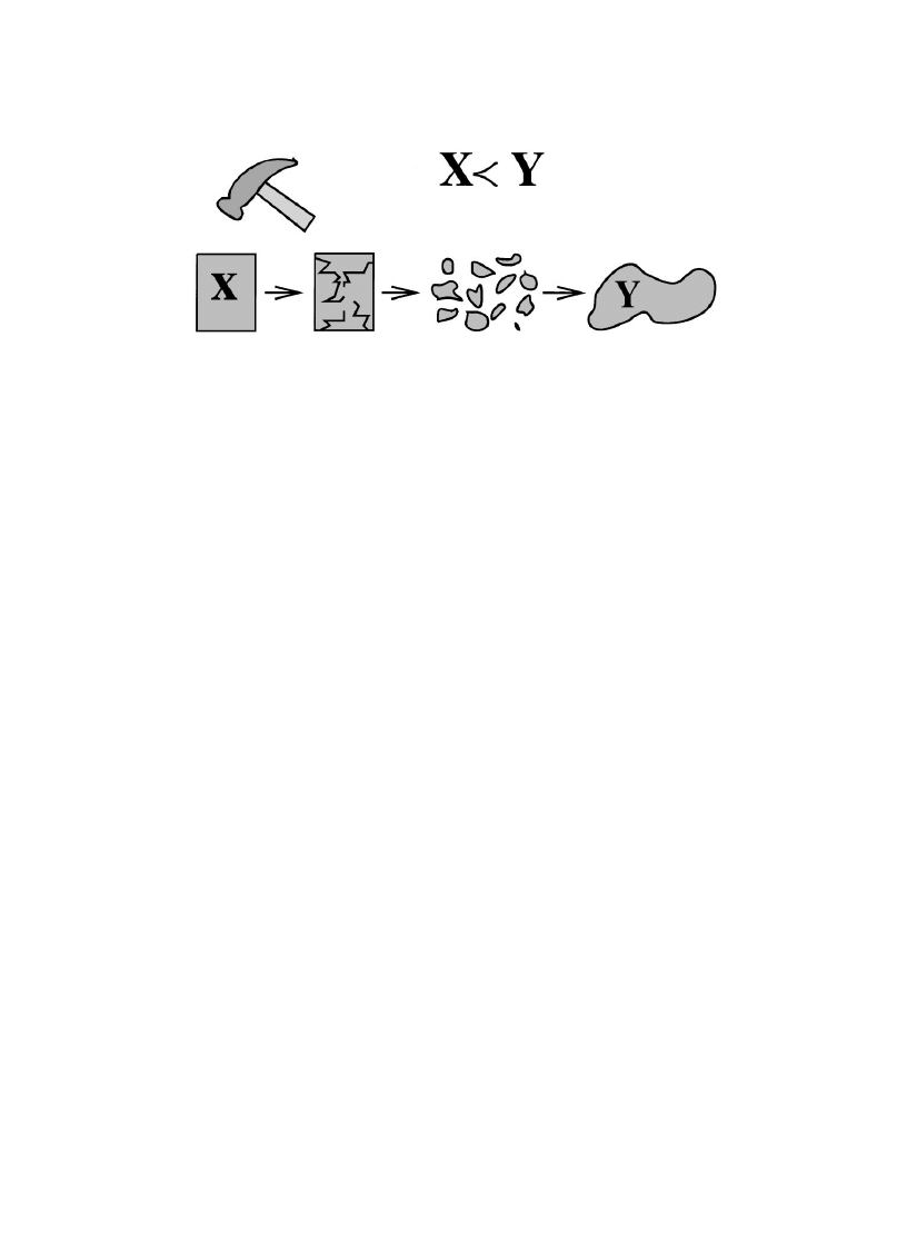
Fig. 1. An example of a violent adiabatic process. The system in an equilibrium state X is transformed by mechanical
means to another equilibrium state ½.

4. Natural processes that occur within an isolated compound system after some barriers have been

removed. This includes mixing and chemical or nuclear processes.

5. Breaking a system into pieces with a hammer and reassembling (Fig. 1).
6. Combinations of such changes.

In the usual parlance, rubbing would be an adiabatic process, but not electrical ‘heating’, because

the latter requires the introduction of a pair of wires through the ‘adiabatic enclosure’. For us, both
processes are adiabatic because what is required is that apart from the change of the system itself,
nothing more than the displacement of a weight occurs. To achieve electrical heating, one drills
a hole in the container, passes a heater wire through it, connects the wires to a generator which, in
turn, is connected to a weight. After the heating the generator is removed along with the wires, the
hole is plugged, and the system is observed to be in a new state. The generator, etc. is in its old state
and the weight is lower.

We shall use the following terminology concerning any two states X and ½. These states are said

to be comparable (with respect to the relation

O, of course) if either XO½ or ½OX. If both

relations hold we say that X and ½ are adiabatically equivalent and write

& ½

(2.2)

The comparison hypothesis referred to above is the statement that any two states in the same state
space are comparable. In the examples of systems (a)—(f) above, all satisfy the comparison
hypothesis. Moreover, every point in

CA is in the relation O to many (but not all) points in CB.

States in different systems may or may not be comparable. An example of non-comparable systems
is one mole of H and one mole of O. Another is one mole of H and two moles of H.

One might think that if the comparison hypothesis, which will be discussed further in Sec-

tions 2.3 and 2.5, were to fail for some state space then the situation could easily be remedied
by breaking up the state space into smaller pieces inside each of which the hypothesis holds.
This, generally, is false. What is needed to accomplish this is the extra requirement that com-
parability is an equivalence relation; this, in turn, amounts to saying that the condition X

and ½

OZ implies that X and ½ are comparable and, likewise, the condition ZOX and

O½ implies that X and ½ are comparable. (This axiom can be found in Giles (1964), see

E.H. Lieb, J. Yngvason / Physics Reports 310 (1999) 1—96

axiom 2.1.2, and similar requirements were made earlier by Landsberg (1956), Falk and Jung
(1959) and Buchdahl (1962, 1966).) While these two conditions are logically independent, they
can be shown to be equivalent if the axiom A3 in Section 2.3 is adopted. In any case, we do not
adopt the comparison hypothesis as an axiom because we find it hard to regard it as a physical
necessity. In the same vein, we do not assume that comparability is an equivalence relation (which
would then lead to the validity of the comparison hypothesis for suitably defined subsystems). Our
goal is to prove the comparison hypothesis starting from axioms that we find more appealing
physically.

2.2. The entropy principle

Given the relation

O for all possible states of all possible systems, we can ask whether this

relation can be encoded in an entropy function according to the following principle, which
expresses the second law of thermodynamics in a precise and quantitative way:

Entropy principle: ¹here is a real-valued function on all states of all systems (including compound

systems), called entropy and denoted by S such that

(a)

Monotonicity: ¼hen X and ½ are comparable states then

O½ if and only if S(X)4S(½) .

(2.3)

(See (2.6) below.)

(b)

Additivity and extensivity: If X and ½ are states of some (possibly different) systems and if (X,½)
denotes the corresponding state in the composition of the two systems, then the entropy is additive
for these states, i.e.,

S((X,½))"S(X)#S(½) .

(2.4)

S is also extensive, i.e., for each t'0 and each state X and its scaled copy tX,

S(tX)"tS(X) .

(2.5)

[Note: From now on we shall omit the double parenthesis and write simply S(X,½) in place of
S((X,½)).]

A logically equivalent formulation of (2.3), that does not use the word ‘comparable’ is the

following pair of statements:

& ½N

S(X)"S(½) ,

(2.6)

OO½NS(X)(S(½) .

The last line is especially noteworthy. It says that entropy must increase in an irreversible process.

Our goal is to construct an entropy function that satisfies the criteria (2.3)—(2.5), and to show that

it is essentially unique. We shall proceed in stages, the first being to construct an entropy function
for a single system,

C, and its multiple scaled copies (in which comparability is assumed to hold).

Having done this, the problem of relating different systems will then arise, i.e., the comparison
question for compound systems. In the present Section 2 (and only in this section) we shall simply

E.H. Lieb, J. Yngvason / Physics Reports 310 (1999) 1—96

complete the project by assuming what we need by way of comparability. In Section 4, the thermal
axioms (the zeroth law of thermodynamics, in particular) will be invoked to verify our assumptions
about comparability in compound systems. In the remainder of this subsection we discuss the
significance of conditions (2.3)—(2.5).

The physical content of Eq. (2.3) was already commented on; adiabatic processes not only

increase entropy but an increase of entropy also dictates which adiabatic processes are possible
(between comparable states, of course).

The content of additivity, Eq. (2.4), is considerably more far reaching than one might think from

the simplicity of the notation — as we mentioned earlier. Consider four states X, X

,½,½ and

suppose that X

O½ and XO½. Then (and this will be one of our axioms) (X, X)O(½,½), and

Eq. (2.4) contains nothing new in this case. On the other hand, the compound system can well have
an adiabatic process in which (X, X

)O(½,½) but XO.½. In this case, Eq. (2.4) conveys much

information. Indeed, by monotonicity, there will be many cases of this kind because the inequality
S(X)#S(X

)4S(½)#S(½) certainly does not imply that S(X)4S(½). The fact that the inequality

S(X)#S(X

)4S(½)#S(½) tells us exactly which adiabatic processes are allowed in the com-

pound system (assuming comparability), independent of any detailed knowledge of the manner in
which the two systems interact, is astonishing and is at the heart of thermodynamics.

Extensivity, Eq. (2.5), is almost a consequence of Eq. (2.4) alone — but logically it is independent.

Indeed, Eq. (2.4) implies that Eq. (2.5) holds for rational numbers t provided one accepts the notion
of recombination as given in Axiom A5 below, i.e., one can combine two samples of a system in the
same state into a bigger system in a state with the same intensive properties. (For systems, such as
cosmic bodies, that do not obey this axiom, extensivity and additivity are truly independent
concepts.) On the other hand, using the axiom of choice, one may always change a given entropy
function satisfying Eqs. (2.3) and (2.4) in such a way that Eq. (2.5) is violated for some irrational t,
but then the function t

| S(tX) would end up being unbounded in every t interval. Such pathologi-

cal cases could be excluded by supplementing Eqs. (2.3) and (2.4) with the requirement that S(tX)
should locally be a bounded function of t, either from below or above. This requirement, plus (2.4),
would then imply Eq. (2.5). For a discussion related to this point see Giles (1964), who effectively
considers only rational t. See also Hardy et al. (1934) for a discussion of the concept of Hamel bases
which is relevant in this context.

The extensivity condition can sometimes have surprising results, as in the case of electromagnetic

radiation (the ‘photon gas’). As is well known (Landau and Lifschitz, 1969, Section 60), the phase
space of such a gas (which we imagine to reside in a box with a piston that can be used to change
the volume) is the quadrant

C"+(º, »): 0(º(R, 0(»(R,. Thus,

CR"C

as sets, which is not surprising or even exceptional. What is exceptional is that S

, which gives the

entropy of the states in

C, satisfies

(º, »)"(const.) »

º .

It is homogeneous of first degree in the coordinates and, therefore, the extensivity law tells us that
the entropy function on the scaled copy

CR is

(º, »)"tS

(º/t,»/t)"S

(º, ») .

E.H. Lieb, J. Yngvason / Physics Reports 310 (1999) 1—96

Thus, all the thermodynamic functions on the two state spaces are the same! This unusual
situation could, in principle, happen for an ordinary material system, but we know of no
example besides the photon gas. Here, the result can be traced to the fact that particle number
is not conserved, as it is for material systems, but it does show that one should not jump
to conclusions. There is, however, a further conceptual point about the photon gas which is
physical rather than mathematical. If a material system had a homogeneous entropy (e.g.,
S(º, »)"(const.) »

º) we should still be able to distinguish CR from C, even though the

coordinates and entropy were indistinguishable. This could be done by weighing the two
systems and finding out that one weighs t times as much as the other. But the photon gas is
different: no experiment can tell the two apart. However, weight per se plays no role in thermo-
dynamics, so the difference between the material and photon systems is not thermodynamically
significant.

There are two points of view one could take about this anomalous situation. One is to continue

to use the state spaces

CR, even though they happen to represent identical systems. This is not

really a problem because no one said that

CR had to be different from C. The only concern is to

check the axioms, and in this regard there is no problem. We could even allow the additive entropy
constant to depend on t, provided it satisfies the extensivity condition (2.5). The second point of
view is to say that there is only one

C and no CR’s at all. This would cause us to consider the photon

gas as outside our formalism and to require special handling from time to time. The first alternative
is more attractive to us for obvious reasons. The photon gas will be mentioned again in connection
with Theorem 2.5.

2.3. Assumptions about the order relation

We now list our assumptions for the order relation

O. As always, X, ½, etc. will denote states

(that may belong to different systems), and if X is a state in some state space

C, then tX with t'0 is

the corresponding state in the scaled state space

CR.

(A1) Reflexivity. X

(A2) Transitivity. X

O½ and ½OZ implies XOZ.

(A3) Consistency. X

OX and ½O½ implies (X,½)O(X,½).

(A4) Scaling invariance. If X

O½, then tXOt½ for all t'0.

(A5) Splitting and recombination. For 0(t(1

(tX, (1!t)X) .

(2.7)

(If X3

C, then the right side is in the scaled product CR;C\R, of course.)

(A6) Stability. If, for some pair of states, X and ½,

(X,

eZ)O(½,eZ)

holds for a sequence of

e’s tending to zero and some states Z, Z, then

O½ .

E.H. Lieb, J. Yngvason / Physics Reports 310 (1999) 1—96

Remark. ‘Stability’ means simply that one cannot increase the set of accessible states with an
infinitesimal grain of dust.

Besides these axioms the following property of state spaces, the ‘comparison hypothesis’, plays

a crucial role in our analysis in this section. It will eventually be established for all state spaces after
we have introduced some more specific axioms in later sections.

Definition. ¼e say the comparison hypothesis (CH) holds for a state space if any two states X and

in the space are comparable, i.e., X

O½ or ½OX.

In the next subsection we shall show that, for every state space,

C, assumptions A1—A6, and CH

for all two-fold scaled products, (1!

j)C;jC, not just C itself, are in fact equivalent to the existence

of an additive and extensive entropy function that characterizes the order relation on the states in
all scaled products of

C. Moreover, for each C, this function is unique, up to an affine transforma-

tion of scale, S(X)PaS(X)#B. Before we proceed to the construction of entropy we derive
a simple property of the order relation from assumptions A1—A6, which is clearly necessary if the
relation is to be characterized by an additive entropy function.

Theorem 2.1 (Stability implies cancellation law). Assume properties A1—A6, especially A6 — the
stability law. ¹hen the cancellation law holds as follows. If X,½ and Z are states of three (possibly
distinct) systems then

(X, Z)

O(½, Z) implies XO½

(Cancellation Law) .

Proof. Let

e"1/n with n"1, 2, 3,

2. Then we have

(X,

eZ)

((1!

e)X, eX, eZ)

(by A5)

O((1!e)X, e½, eZ)

(by A1, A3 and A4)

((1!2

e)X, eX, e½, eZ) (by A5)

O((1!2e)X, 2e½, eZ)

(by A1, A3—A5).

By doing this n"1/

e times we find that (X, e Z)O(½, e Z). By the stability axiom A6 we then have

O½.

䊏

Remark. Under the additional assumption that ½ and Z are comparable states (e.g., if they are in
the same state space for which CH holds), the cancellation law is logically equivalent to the
following statement (using the consistency axiom A3):

If X

OO½ then (X, Z)OO(½, Z) for all Z.

The cancellation law looks innocent enough, but it is really rather strong. It is a partial converse of
the consistency condition A3 and it says that although the ordering in

C;C is not determined

E.H. Lieb, J. Yngvason / Physics Reports 310 (1999) 1—96

simply by the order in

C and C, there are limits to how much the ordering can vary beyond the

minimal requirements of A3. It should also be noted that the cancellation law is in accord with
our physical interpretation of the order relation in Section 2.1.2; a ‘spectator’, namely Z, cannot
change the states that are adiabatically accessible from X.

Remark about ‘Adiabatic Processes’. With the aid of the cancellation law we can now discuss the
connection between our notion of adiabatic accessibility and the textbook concept of an ‘adiabatic
process’. One problem we face is that this latter concept is hard to make precise (this was our
reason for avoiding it in our operational definition) and therefore the discussion must necessarily
be somewhat informal. The general idea of an adiabatic process, however, is that the system of
interest is locked in a thermally isolating enclosure that prevents ‘heat’ from flowing into or out of
our system. Hence, as far as the system is concerned, all the interaction it has with the external
world during an adiabatic process can be thought of as being accomplished by means of some
mechanical or electrical devices. Our operational definition of the relation

O appears at first sight

to be based on more general processes, since we allow an auxiliary thermodynamical system as part
of the device. We shall now show that, despite appearances, our definition coincides with the
conventional one.

Let us temporarily denote by

OH the relation between states based on adiabatic processes, i.e.,

OH½ if and only if there is a mechanical/electrical device that starts in a state M and ends up in

a state M

while the system changes from X to ½. We now assume that the mechanical/electrical

device can be restored to the initial state M from the final state M

by adding or substracting

mechanical energy, and this latter process can be reduced to the raising or lowering of a weight in
a gravitational field. (This can be taken as a definition of what we mean by a ‘mechanical/electrical
device’. Note that devices with ‘dissipation’ do not have this property.) Thus, X

OH½ means there is

a process in which the mechanical/electrical device starts in some state M and ends up in the same
state, a weight moves from height h to height h

, while the state of our system changes from X to ½.

In symbols,

(X, M, h)P(½, M, h

) .

(2.8)

In our definition of adiabatic accessibility, on the other hand, we have some arbitrary device,

which interacts with our system and which can generate or remove heat if desired. There is no
thermal enclosure. The important constraint is that the device starts in some state D and ends up in
the same state D. As before a weight moves from height h to height h

, while our system starts in

state X and ends up in state ½. In symbols,

(X, D, h)P(½, D, h

) .

(2.9)

It is clear that (2.8) is a special case of (2.9), so we conclude that X

OH½ implies XO½. The device in

(2.9) may consist of a thermal part in some state Z and electrical and mechanical parts in some state
M. Thus D"(Z, M), and (2.9) clearly implies that (X, Z)

OH(½, Z).

It is natural to assume that

OH satisfies axioms A1—A6, just as O does. In that case we can infer

the cancellation law for

OH, i.e., (X, Z)OH(½, Z) implies XOH½. Hence, XO½ (which is what (2.9)

says) implies X

OH½. Altogether we have thus shown that O and OH are really the same relation.

In words: adiabatic accessibility can always be achieved by an adiabatic process applied to the system

E.H. Lieb, J. Yngvason / Physics Reports 310 (1999) 1—96

plus a device and, furthermore, the adiabatic process can be simplified (although this may not be easy
to do experimentally) by eliminating all thermodynamic parts of the device, thus making the process an
adiabatic one for the system alone.

2.4. The construction of entropy for a single system

Given a state space

C we may, as discussed in Section 2.1.1, construct its multiple scaled copies,

i.e., states of the form

½"

(t½,2, t,½,)

with tG'0, ½G3C. It follows from our assumption A5 that if CH (comparison hypothesis) holds in

the state space

;2;CR

with t,2,t, fixed, then any other state of the same form,

"(t½,2,t+½+) with ½G3C, is comparable to ½ provided

tG"

H (but not, in general, if

the sums are not equal). This is proved as follows for N"M"2; the easy extension to the general
case is left to the reader. Since t#t"t#t we can assume, without loss of generality, that

t!t"t!t'0, because the case t!t"0 is already covered by CH (which was assumed)

for

;CR

. By the splitting axiom, A5, we have (t½,t½) & (t½,(t!t)½,t½) and

½,t½) & (t½,(t!t)½,t½). The comparability now follows from CH on the space

;CR

The entropy principle for the states in the multiple scaled copies of a single system will now be

derived. More precisely, we shall prove the following theorem:

Theorem 2.2 (Equivalence of entropy and assumptions A1–A6, CH). ¸et

C be a state space and let

O be a relation on the multiple scaled copies of C. ¹he following statements are equivalent.

(1)

he relation

O satisfies axioms A1—A6, and CH holds for all multiple scaled copies of C.

(2)

here is a function, S

C that characterizes the relation in the sense that if

t#2#t,"t#2#t+, (for all N51 and M51) then

(t½,2, t,½,)O(t½,2,t+½+)

holds if and only if

tGS

(½G)4

(½

H) .

(2.10)

he function S

is uniquely determined on

C, up to an affine transformation, i.e., any other function

C satisfying (2.10) is of the form SH

(X)"aS

(X)#B with constants a'0 and B.

Definition. A function S

C that characterizes the relation O on the multiple scaled copies of

C in the sense stated in the theorem is called an entropy function on C.

We shall split the proof of Theorem 2.2 into Lemmas 2.1—2.3 and Theorem 2.3 below.
At this point it is convenient to introduce the following notion of generalized ordering. While

(aX, aX,2, a,X,) has so far only been defined when all aG'0, we can define the meaning of

E.H. Lieb, J. Yngvason / Physics Reports 310 (1999) 1—96

the relation

(aX,2, a,X,)O(aX,2,a+X+)

(2.11)

for arbitrary aG3R, aG3R, N and M positive integers and XG3CG, XG3CG as follows. If any aG (or aG) is

zero we just ignore the corresponding term. Example: (0X, X)O(2X, 0X) means the same thing

as XO2X. If any aG (or aG) is negative, just move aGXG (or aGXG) to the other side and change the

sign of aG (or aG). Example:

(2X, X)O(X,!5X,2X, X)

means that

(2X, 5X, X)O(X,2X, X)

and

C;C;C. (Recall that C?;C@"C@;C?.) It is easy to check, using the

cancellation law, that the splitting and recombination axiom A5 extends to nonpositive scaling
parameters, i.e., axioms A1—A6 imply that X

(aX, bX) for all a, b3R with a#b"1, if the

relation

O for nonpositive a and b is understood in the sense just described.

For the definition of the entropy function we need the following lemma, which depends crucially

on the stability assumption A6 and on the comparison hypothesis CH for the state spaces
C\H;CH.

Lemma 2.1. Suppose X and X are two points in C with XOOX. For j3R define

SH"+X3C:((1!j)X, jX)OX, .

(2.12)

hen

(i)

For every X3

C there is a j3R such that X3SH.

(ii)

For every X3

C, sup+j: X3SH,(R.

Remark. Since X

((1!

j)X, jX) by assumption A5, the definition of SH really involves the

order relation on double scaled copies of

C (or on C itself, if j"0 or 1.)

Proof of Lemma 2.1. (i) If XOX then obviously X3S by axiom A2. For general X we claim that

(1#

a)XO(aX,X)

(2.13)

for some

a50 and hence ((1!j)X,jX)OX with j"!a. The proof relies on stability, A6, and

the comparison hypothesis CH (which comes into play for the first time): If (2.13) were not true,
then by CH we would have

(

aX,X)O(1#a)X

for all

a'0 and so, by scaling, A4, and A5

1
a

By the stability axiom A6 this would imply XOX in contradiction to XOOX.

E.H. Lieb, J. Yngvason / Physics Reports 310 (1999) 1—96

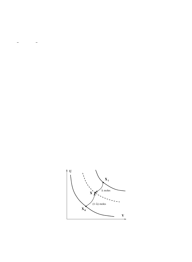
Fig. 2. The entropy of a state X is determined, according to formula 2.14, by the amount of substance in state X that can

be transformed down to X with the aid of a complementary amount of substance in the state X.

(ii) If sup

+j: X3SH,"R, then for some sequence of j’s tending to infinity we would have

((1!

j)X,jX)OX and hence (X,jX)O(X,jX) by A3 and A5. By A4 this implies

(

HX,X)O(HX,X) and hence XOX by stability, A6.

䊏

We can now state our formula for the entropy function. If all points in

C are adiabatically

equivalent there is nothing to prove (the entropy is constant), so we may assume that there are
points X, X3C with XOOX. We then define for X3C

(X) :"sup

+j: ((1!j)X,jX)OX, .

(2.14)

(The symbol a :"b means that a is defined by b.) This S

will be referred to as the canonical entropy

C with reference points X and X. This definition is illustrated in Fig. 2.

By Lemma 2.1 S

(X) is well defined and S

(X)(R for all X. (Note that by stability we could

replace

O by OO in (2.14).) We shall now show that this S

has all the right properties. The first

step is the following simple lemma, which does not depend on the comparison hypothesis.

Lemma 2.2 (

O is equivalent to 4). Suppose XOOX are states and a, a, a, a are real numbers

with a#a"a#a. ¹hen the following are equivalent.
(i)

(aX, aX)O(aX, aX)

(ii)

a4a (and hence a5a).

In particular,

holds in (i) if and only if a"a and a"a.

Proof. We give the proof assuming that the numbers a, a, a, a are all positive and a#a"

#a"1. The other cases are similar. We write a"j and a"j.

(i) N (ii). If

j'j then, by A5 and A3, ((1!j)X, jX, (j!j)X)O((1!j)X,

(

j!j)X, jX). By the cancellation law, Theorem 2.1, ((j!j)X)O((j!j)X). By scaling

invariance, A5, XOX, which contradicts XOOX.

E.H. Lieb, J. Yngvason / Physics Reports 310 (1999) 1—96

(ii) N (i). This follows from the following computation.

((1!

j)X, jX) & ((1!j)X, (j!j)X,jX) (by axioms A3 and A5)

O((1!j)X, (j!j)X,jX) (by axioms A3 and A4)

((1!

j)X,jX)

(by axioms A3 and A5) .

䊏

The next lemma will imply, among other things, that entropy is unique, up to an affine transforma-
tion.

Lemma 2.3 (Characterization of entropy). ¸et S

denote the canonical entropy (2.14) on

C with

respect to the reference points XOOX. If X3C then the equality

j"S

(X)

is equivalent to

((1!

j)X,jX) .

Proof. First, if

j"S

(X) then, by the definition of supremum, there is a sequence

e5e5250

converging to zero, such that

((1!(

j!eL))X,(j!eL)X)OX

for each n. Hence, by A5,

((1!

j)X,jX,eLX) & ((1!j#eL)X,(j!eL)X,eLX)O(X,eLX) ,

and thus ((1!

j)X,jX)OX by the stability property A6. On the other hand, since j is the

supremum we have

O((1!(j#e)X,(j#e)X)

for all

e'0 by the comparison hypothesis CH. Thus,

(X,

eX)O((1!j)X,jX,eX) ,

so, by A6, X

O((1!j)X,jX). This shows that X & ((1!j)X,jX) when j"S

(X).

Conversely, if

j3[0, 1] is such that X

((1!

j)X,jX), then ((1!j)X,jX) &

((1!

j)X,jX) by transitivity. Thus, j"j by Lemma 2.2.

䊏

Remark 1. Without the comparison hypothesis we could find that S

(X)"0 and S

(X)"1 for all

X such that XOX.

Remark 2. From Lemma 2.3 and the cancellation law it follows that the canonical entropy with
reference points XOOX satisfies 04S

(X)41 if and only if X belongs to the strip

R(X,X)

defined by

R(X,X) :"+X3C: XOXOX,LC .

E.H. Lieb, J. Yngvason / Physics Reports 310 (1999) 1—96

Let us make the dependence of the canonical entropy on X and X explicit by writing

(X)"S

"X,X) .

(2.15)

For X outside the strip we can then write

"X,X)"S

(X"X, X)\ if XOX

and

"X,X)"!

(X"X,X)

1!S

(X"X,X)

if X

OX .

Proof of Theorem 2.2. (1) N (2): Put

jG"S

(½G), jG"S

(½

G). By Lemma 2.3 we know that

½G

((1!

jG)X,jGX) and ½G & ((1!jG)X,jGX). By the consistency axiom A3 and the recom-

bination axiom A5 it follows that

(t½,2, t,½,)

tG(1!jG)X,

tGjGX

½,2,t,½,) &

G(1!jG)X,

GjGX

Statement (2) now follows from Lemma 2.2. The implication (2) N (1) is obvious.

The proof of Theorem 2.2 is now complete except for the uniqueness part. We formulate this part

separately in Theorem 2.3 below, which is slightly stronger than the last assertion in Theorem 2.2.
It implies that an entropy function for the multiple scaled copies of

C is already uniquely

determined, up to an affine transformation, by the relation on states of the form ((1!

j)X, j½), i.e.,

it requires only the case N"M"2, in the notation of Theorem 2.2.

Theorem 2.3 (Uniqueness of entropy). If S

is a function on

C that satisfies

((1!

j)X, j½)O((1!j)X, j½)

if and only if

(1!

j)SH

(X)#

jSH

(½)4(1!

j)SH

)#jSH

(½

) ,

for all

j3R and X, ½, X, ½3C, then

(X)"aS

(X)#B

with

a"S

(X)!SH

(X)'0, B"SH

(X) .

Here S

is the canonical entropy on

C with reference points XOOX.

Proof. This follows immediately from Lemma 2.3, which says that for every X there is a unique

namely

j"S

(X), such that

((1!

j)X, jX)

((1!

j)X,jX) .

E.H. Lieb, J. Yngvason / Physics Reports 310 (1999) 1—96

Hence, by the hypothesis on S

, and

j"S

(X), we have

(X)"(1!

j)SH

(X)#jSH

(X)"[SH

(X)!SH

(X)]S

(X)#S

(X) .

The hypothesis on S

also implies that a :"S

(X)!SH

(X)'0, because XOOX.

䊏

Remark. Note that S

is defined on

C and satisfies SH

(X)"aS

(X)#B there. On the space

CR a corresponding entropy is, by definition, given by SH

(tX)"tS

(X)"atS

(X)#tB"

(tX)#tB, where S

(tX) is the canonical entropy on

CR with reference points tX,tX. Thus,

(tX)OaS

(tX)#B (unless B"0, of course).

It is apparent from formula (2.14) that the definition of the canonical entropy function on

C involves only the relation O on the double scaled products C\H;CH besides the reference
points X and X. Moreover, the canonical entropy uniquely characterizes the relation on all

multiple scaled copies of

C, which implies in particular that CH holds for all multiple scaled copies.

Theorem 2.3 may therefore be rephrased as follows:

Theorem 2.4 (The relation on double scaled copies determines the relation everywhere). ¸et

O and

OH be two relations on the multiple scaled copies of C satisfying axioms A1—A6, and also CH for

C\H;CH for each fixed j3[0, 1]. If O and OH coincide on C\H;CH for each j3[0, 1], then

O and OH coincide on all multiple scaled copies of C, and CH holds on all the multiple scaled copies.

The proof of Theorem 2.2 is now complete.

2.5. Construction of a universal entropy in the absence of mixing

In the previous subsection we showed how to construct an entropy for a single system,

C, that

exactly describes the relation

O within the states obtained by forming multiple scaled copies of C.

It is unique up to a multiplicative constant a'0 and an additive constant B, i.e., to within an affine
transformation. We remind the reader that this entropy was constructed by considering just the
product of two scaled copies of

C, but our axioms implied that it automatically worked for all

multiple scaled copies of

C. We shall refer to a and B as entropy constants for the system C.

Our goal is to put these entropies together and show that they behave in the right way on

products of arbitrarily many copies of different systems. Moreover, this ‘universal’ entropy will be
unique up to one multiplicative constant — but still many additive constants. The central question
here is one of ‘calibration’, which is to say that the multiplicative constant in front of each
elementary entropy has to be chosen in such a way that the additivity rule (2.4) holds. It is not even
obvious yet that the additivity can be made to hold at all, whatever the choice of constants.

Let us note that the number of additive constants depends heavily on the kinds of adiabatic

processes available. The system consisting of one mole of hydrogen mixed with one mole of helium
and the system consisting of one mole of hydrogen mixed with two moles of helium are different.
The additive constants are independent unless a process exists in which both systems can be
unmixed, and thereby making the constants comparable. In nature we expect only 92 constants,
one for each element of the periodic table, unless we allow nuclear processes as well, in which case

E.H. Lieb, J. Yngvason / Physics Reports 310 (1999) 1—96

there are only two constants (for neutrons and for hydrogen). On the other hand, if un-mixing is not
allowed uncountably many constants are undetermined. In Section 6 we address the question of
adiabatic processes that unmix mixtures and reverse chemical reactions. That such processes exist
is not so obvious.

To be precise, the principal goal of this subsection is the proof of the following Theorem 2.5,

which is a case of the entropy principle that is special in that it is restricted to processes that do not
involve mixing or chemical reactions. It is a generalization of Theorem 2.2.

Theorem 2.5 (Consistent entropy scales). Consider a family of systems fulfilling the following
requirements:

(i)

he state spaces of any two systems in the family are disjoint sets, i.e., every state of a system in

the family belongs to exactly one state space.

(ii)

All multiple scaled products of systems in the family belong also to the family.

(iii) Every system in the family satisfies the comparison hypothesis.

For each state space

C of a system in the family let S

be some definite entropy function on

C. ¹hen

there are constants a

and B

such that the function S, defined for all states in all

C’s by

S(X)"a

(X)#B

for X3

C, has the following properties:

(a)

If X and ½ are in the same state space then

O½ if and only if S(X)4S(½) .

(b)

S is additive and extensive, i.e.,

S(X,½)"S(X)#S(½) .

(2.4

)

and, for t'0,

S(tX)"tS(X) .

(2.5

)

Remark. Note that

C and C;C are disjoint as sets for any (nonempty) state spaces C and C.

Proof. Fix some system

C and two points ZOOZ in C. In each state space C choose some

fixed point X

C in such a way that the identities

, X

) ,

(2.16)

(2.17)

hold. With the aid or the axiom of choice this can be achieved by considering the formal vector
space spanned by all systems and choosing a Hamel basis of systems

+C?, in this space such that

every system can be written uniquely as a scaled product of a finite number of the

C?’s (see Hardy et

al., 1934). The choice of an arbitrary state X

in each of these ‘elementary’ systems

C? then defines

for each

C a unique X

such that Eq. (2.17) holds. (If the reader does not wish to invoke the axiom

of choice then an alternative is to hypothesize that every system has a unique decomposition into

E.H. Lieb, J. Yngvason / Physics Reports 310 (1999) 1—96

elementary systems; the simple systems considered in the next section obviously qualify as the
elementary systems.)

For X3

C we consider the space C;C with its canonical entropy as defined in (2.14), (2.15)

relative to the points (X

, Z) and (X

, Z). Using this function we define

S(X)"S

((X, Z) "(X

, Z),(X

, Z)) .

(2.18)

Note: Eq. (2.18) fixes the entropy of X

to be zero.

Let us denote S(X) by

j which, by Lemma 2.3, is characterized by

(X, Z)

((1!

j)(X

, Z),j(X

, Z)) .

By the cancellation law this is equivalent to

(X,

jZ) & (X

jZ) .

(2.19)

By Eqs. (2.16) and (2.17) this immediately implies the additivity and extensivity of S. Moreover,

since X

O½ holds if and only if (X, Z)O(½,Z) it is also clear that S is an entropy function on any

C. Hence S and S

are related by an affine transformation, according to Theorem 2.3.

䊏

Definition (Consistent entropies). A collection of entropy functions S

on state spaces

C is called

consistent if the appropriate linear combination of the functions is an entropy function on all
multiple scaled products of these state spaces. In other words, the set is consistent if the multiplica-
tive constants a

, referred to in Theorem 2.5, can all be chosen equal to 1.

Important Remark: From the definition, Eq. (2.14), of the canonical entropy and Eq. (2.19) it

follows that the entropy (2.18) is given by the formula

S(X)"sup

+j: (X

jZ)O(X,jZ),

(2.20)

for X3

C. The auxiliary system C can thus be regarded as an ‘entropy meter’ in the spirit of Lewis

and Randall (1923) and Giles (1964). Since we have chosen to define the entropy for each system
independently, by Eq. (2.14), the role of

C in our approach is solely to calibrate the entropy of

different systems in order to make them consistent.

Remark about the photon gas. As we discussed in Section 2.2 the photon gas is special and there are
two ways to view it. One way is to regard the scaled copies

CR as distinct systems and the other is to

say that there is only one

C and the scaled copies are identical to it and, in particular, must have

exactly the same entropy function. We shall now see how the first point of view can be reconciled
with the latter requirement. Note, first, that in our construction above we cannot take the point
(º, »)"(0, 0) to be the fiducial point X

because (0, 0) is not in our state space which, according to

the discussion in Section 3 below, has to be an open set and hence cannot contain any of its
boundary points such as (0, 0). Therefore, we have to make another choice, so let us take X

(1, 1).

But the construction in the proof above sets S

(1, 1)"0 and therefore S

(º, ») will not have the

homogeneous form S

(º, »)"»º. Nevertheless, the entropies of the scaled copies will

be extensive, as required by the theorem. If one feels that all scaled copies should have the same
entropy (because they represent the same physical system) then the situation can be remedied in the

E.H. Lieb, J. Yngvason / Physics Reports 310 (1999) 1—96

following way: With S

(º, ») being the entropy constructed as in the proof using(1, 1), we note that

(º, »)"S

(º, »)#B

with the constant B

given by B

(2, 2). This follows from

simple algebra and the fact that we know that the entropy of the photon gas constructed in our
proof must equal S

to within an additive constant. (The reader might ask how we know this and

the answer is that the entropy of the ‘gas’ is unique up to additive and multiplicative constants, the
latter being determined by the system of units employed. Thus, the entropy determined by our
construction must be the ‘correct entropy’, up to an additive constant, and this ‘correct entropy’ is
what it is, as determined by physical measurement. Hopefully it agrees with the function deduced in
Landau and Lifschitz (1969).) Let us use our freedom to alter the additive constants as we please,
provided we maintain the extensivity condition (2.5). It will not be until Section 6 that we have to
worry about the additive constants per se because it is only there that mixing and chemical
reactions are treated. Therefore, we redefine the entropy of the state space

C of the photon gas

to be S

H(º, ») :"S

(º, »)#S

(2, 2) which is the same as S

(º, »). We also have to alter the

entropy of the scaled copies according to the rule that preserves extensivity, namely
S

(º, »)PS

(º, »)#tS

(2, 2)"S

(º, »)#S

(2t, 2t)"S

(º, »). In this way, all the scaled

copies now have the same (homogeneous) entropy, but we remind the reader that the same
construction could be carried out for any material system with a homogeneous (or, more exactly an
affine) entropy function — if one existed. From the thermodynamic viewpoint, the photon gas is
unusual but not special.

2.6. Concavity of entropy

Up to now we have not used, or assumed, any geometric property of a state space

C. It is an

important stability property of thermodynamical systems, however, that the entropy function is
a concave function of the state variables — a requirement that was emphasized by Maxwell, Gibbs,
Callen and many others. Concavity also plays an important role in the definition of temperature, as
in Section 5.

In order to have this concavity it is first necessary to make the state space on which entropy is

defined into a convex set, and for this purpose the choice of coordinates is important. Here, we
begin the discussion of concavity by discussing this geometric property of the underlying state
space and some of the consequences of the convex combination axiom A7 for the relation

O, to be

given after the following definition.

Definition. By a state space with a convex structure, or simply a convex state space, we mean a state
space

C, that is a convex subset of some linear space, e.g., RL. That is, if X and ½ are any two points

C and if 04t41, then the point tX#(1!t)½ is a well-defined point in C. A concave function,

S, on

C is one satisfying the inequality

S(tX#(1!t)½)5tS(X)#(1!t)S(½) .

(2.21)

Our basic convex combination axiom for the relation

O is the following.

(A7) Convex combination. Assume X and ½ are states in the same convex state space,

For t3[0, 1] let tX and (1!t)½ be the corresponding states of their t scaled and (1!t)
scaled copies, respectively. Then the point (tX,(1!t)½) in the product space

CR;C\R

E.H. Lieb, J. Yngvason / Physics Reports 310 (1999) 1—96

satisfies

(tX, (1!t)½)

OtX#(1!t)½ .

(2.22)

Note that the right side of (2.22) is in

C and is defined by ordinary convex combination of

points in the convex set

The physical meaning of A7 is more or less evident, but it is essential to note that the convex

structure depends heavily on the choice of coordinates for

C. A7 means that if we take a bottle

containing 1/4 moles of nitrogen and one containing 3/4 moles (with possibly different pressures
and densities), and if we mix them together, then among the states of one mole of nitrogen that can
be reached adiabatically there is one in which the energy is the sum of the two energies and,
likewise, the volume is the sum of the two volumes. Again, we emphasize that the choice of energy
and volume as the (mechanical) variables with which we can make this statement is an important
assumption. If, for example, temperature and pressure were used instead, the statement would not
only not hold, it would not even make much sense.

The physical example above seems not exceptionable for liquids and gases. On the other hand, it

is not entirely clear how to ascribe an operational meaning to a convex combination in the state
space of a solid, and the physical meaning of axiom A7 is not as obvious in this case. Note, however,
that although convexity is a global property, it can often be inferred from a local property of the
boundary. (A connected set with a smooth boundary, for instance, is convex if every point on the
boundary has a neighbourhood, whose intersection with the set is convex.) In such cases it suffices
to consider convex combinations of points that are close together and close to the boundary. For
small deformation of an isotropic solid the six strain coordinates, multiplied by the volume, can be
taken as work coordinates. Thus, A7 amounts to assuming that a convex combination of these
coordinates can always be achieved adiabatically. See, e.g., Callen (1985).

If X3

C we denote by A6 the set +½3C: XO½,. A6 is called the forward sector of X in C. More

generally, if

C is another system, we call the set

+½3C : XO½, ,

the forward sector of X in

Usually this concept is applied to the case in which

C and C are identical, but it can also be useful

in cases in which one system is changed into another; an example is the mixing of two liquids in two
containers (in which case

C is a compound system) into a third vessel containing the mixture (in

which case

C is simple).

The main effect of A7 is that forward sectors are convex sets.

Theorem 2.6 (Forward sectors are convex). ¸et

C and C be state spaces of two systems, with C

a convex state space. Assume that A1—A5 hold for

C and C and, in addition, A7 holds for C. ¹hen the

forward sector of X in

C, defined above, is a convex subset of C for each X3C.

Proof. Suppose X

O½ and XO½ and that 0(t(1. We want to show that XOt½#

(1!t)½. (The right side defines, by ordinary vector addition, a point in the convex set C.)

First, X

O(tX, (1!t)X)3CR;C\R, by axiom A5. Next, (tX, (1!t)X)O(t½,(1!t)½) by the

E.H. Lieb, J. Yngvason / Physics Reports 310 (1999) 1—96

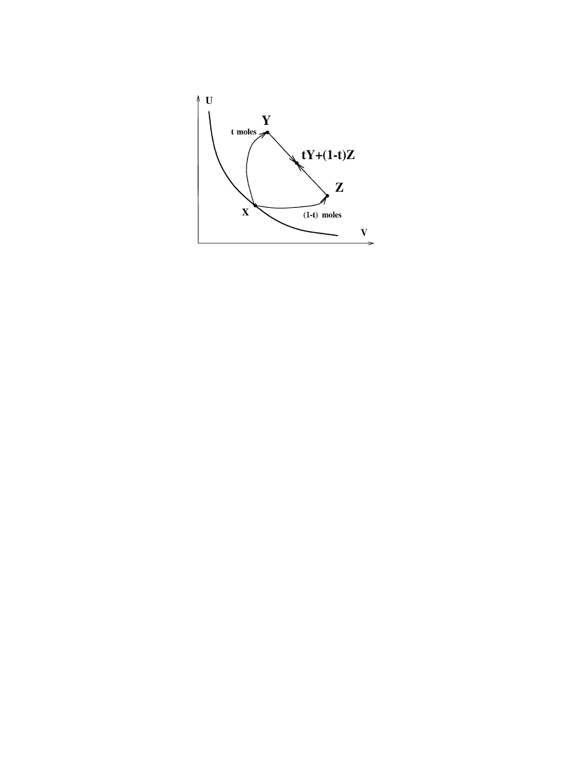
Fig. 3. This illustrates axiom A7 and Theorem 2.6 which says that if states ½ and Z can be reached adiabatically from
a state X and if the state space has a convex structure then convex combinations of ½ and Z are also in the forward sector
of X.

consistency axiom A3 and the scaling invariance axiom A4. Finally, (t½,(1!t)½)Ot½#

(1!t)½ by the convex combination axiom A7.

䊏

Fig. 3 illustrates this theorem in the case

C"C.

Theorem 2.7 (Convexity of SH). ¸et the sets SHLC be defined as in Eq. (2.12) and assume the state

space

C satisfies the convex combination axiom A7 in addition to A1—A5. ¹hen:

(i)

SH is convex.

(ii)

If X3SH

, ½3SH

and 04t41, then tX#(1!t)½3SRH

>\RH

Proof. (i) This follows immediately from the scaling, splitting and convex combination axioms A4,
A5 and A7.

(ii) This is proved by splitting, moving the states of the subsystems into forward sectors and

bringing the subsystems together at the end. More precisely, defining

j"tj#(1!t)j we have

to show that ((1!

j)X,jX)OtX#(1!t)½. Starting with ((1!j)X,jX) we split (1!j)X

into (t(1!

j)X,(1!t)(1!j)X) and jX into (tjX,(1!t)jX). Next we consider the states

(t(1!

j)X,tjX) and ((1!t)(1!j)X,(1!t)jX). By scaling invariance A4 and the splitting

property A5 we can pass from the former to (t(1!

j)X,tjX) and from the latter to

((1!t)(1!

j)½,(1!t)j½). Now we combine the parts of (t(1!j)X,tjX) to obtain tX and the

parts of ((1!t)(1!

j)½,(1!t)j½) to obtain (1!t)½, and finally we use the convex combination

property A7 to reach tX#(1!t)½.

䊏

Theorem 2.8 (Concavity of entropy). ¸et

C be a convex state space. Assume axiom A7 in addition to

A1—A6, and CH for multiple scaled copies of

C. ¹hen the entropy S

defined by (2.14) is a concave

function on

C. Conversely, if S

is concave, then axiom A7 necessarily holds a fortiori.

E.H. Lieb, J. Yngvason / Physics Reports 310 (1999) 1—96

Proof. If X3SH

,½3SH

, then by Theorem 2.7, (ii), tX#(1!t)½3SRH

>\RH

, for t,

j,j3[0,1].

By definition, this implies S

(tX#(1!t)½)5t

j#(1!t)j. Taking the supremum over all

j and j such that X3SH

,½3SH

, then gives S

(tX#(1!t)½)5tS

(X)#(1!t)S

(½). The

converse is obvious.

䊏

2.7. Irreversibility and Carathe´odory’s principle

One of the milestones in the history of the second law is Carathe´odory’s attempt to formulate the

second law in terms of purely local properties of the equivalence relation

. The disadvantage of

the purely local formulation is, as we said earlier, the difficulty of deriving a globally defined
concave entropy function. Additionally, Carathe´odory relies on differentiability (differential forms),
and we would like to avoid this, if possible, because physical systems do have points (e.g., phase
transitions) in their state spaces where differentiability fails. Nevertheless, Carathe´odory’s idea
remains a powerful one and it does play an important role in the story. We shall replace it by
a seemingly more natural idea, namely the existence of irreversible processes. ¹he existence of many
such processes lies at the heart of thermodynamics. If they did not exist, it would mean that nothing is
forbidden, and hence there would be no second law. We now show the relation between the two
concepts. There will be no mention of differentiability, however.

Carathe´odory’s principle has been criticized (see, for example, the remark attributed to Walter in

Truesdell’s paper in Serrin (1986, Chapter 5)) on the ground that this principle does not tell us
where to look for a non adiabatic process that is supposed, by the principle, to exist in every
neighborhood of every state. In Sections 3 and 5 we show that this criticism is too severe because
the principle, when properly interpreted, shows exactly where to look and, in conjunction with the
other axioms, it leads to the Kelvin—Planck version of the second law.

Theorem 2.9 (Carathe´odory’s principle and irreversible processes). ¸et

C be a state space that is

a convex subset of R

L and assume that axioms A1—A7 hold on C. Consider the following two

statements.

(1)

Existence of irreversible processes: For every point X3

C there is a ½3C such that XOO½.

(2)

Carathe´odory’s principle: In every neighborhood of every X3

C there is a point Z3C such that

Z is false.

hen (1) always implies (2). Indeed, (1) implies the stronger statement that there is a Z such that

OZ is false. On the other hand, if all the forward sectors in C have non-empty interiors (i.e., they are

not contained in lower dimensional hyperplanes) then (2) implies (1).

Proof. Suppose that for some X3

C there is a neighborhood, N6 of X such that N6 is contained

in A6, the forward sector of X. (This is the negation of the statement that in every neighbourhood of

every X there is a Z such that X

OZ is false.) Let ½3A6 be arbitrary. By the convexity of A6 (which

is implied by the axioms), X is an interior point of a line segment joining ½ and some point Z3N6.

By axiom A7, we thus have

((1!

j)Z, j½)OX

((1!

j)X, jX)

E.H. Lieb, J. Yngvason / Physics Reports 310 (1999) 1—96

for some

j3(0, 1). But we also have that ((1!j)X, j½)O((1!j)Z, j½) since Z3A6. This implies,

by the cancellation law, that ½

OX. Thus we conclude that for some X, we have that XO½ implies

& ½

. This contradicts (1). In particular, we have shown that (1) N (2).

Conversely, assuming that (1) is false, there is a point X whose forward sector is given by

+½: ½

X,. Let X be an interior point of A6

, i.e., there is a neighborhood of X, N6,

which is entirely contained in A6

. All points in N6 are adiabatically equivalent to X, however,

and hence to X, since X3N6. Thus, (2) is false.

䊏

2.8. Some further results on uniqueness

As stated in Theorem 2.2, the existence of an entropy function on a state space

C is equivalent to

the axioms A1—A6 and CH for the multiple scaled copies of

C. The entropy function is unique, up to

an affine change of scale, and according to formula (2.14) it is even sufficient to know the relation on
the double scaled copies

C\H;CH in order to compute the entropy. This was the observation

behind the uniqueness Theorem 2.4 which stated that the restriction of the relation

O to the double

scaled copies determines the relation everywhere.

The following very general result shows that it is in fact not necessary to know

O on all

C\H;CH to determine the entropy, provided the relation is such that the range of the entropy is
connected. In this case

j"1/2 suffices. By Theorem 2.8 the range of the entropy is necessarily

connected if the convex combination axiom A7 holds.

Theorem 2.10 (The relation on

C;C determines entropy). ¸et C be a set and O a relation on C;C.

et S be a real valued function on

C satisfying the following conditions:

(i)

S characterizes the relation on

C;C in the sense that

(X,½)

O(X,½) if and only if S(X)#S(½)4S(X)#S(½).

(ii)

he range of S is an interval (bounded or unbounded and which could even be a point).

et S

H be another function on C satisfying condition (i). ¹hen S and SH are affinely related, i.e., there

are numbers a'0 and B such that S

H(X)"aS(X)#B for all X3C. In particular, SH must satisfy

condition (ii).

Proof. In general, if F and G are any two real valued functions on

C;C, such that

F(X,½)4F(X

,½) if and only if G(X,½)4G(X,½), it is an easy logical exercise to show that there

is a monotone increasing function K (i.e., x4y implies K(x)4K(y)) defined on the range of F, so
that G"K

F. In our case F(X,½)"S(X)#S(½). If the range of S is the interval ¸ then the range

of F is 2¸. Thus K, which is defined on 2¸, satisfies

K(S(X)#S(½))"S

H(X)#SH(½)

(2.23)

for all X and ½ in

C because both S and SH satisfy condition (i). For convenience, define M on ¸ by

M(t)"

K(2t). If we now set ½"X in (1) we obtain

H(X)"M(S(X)), X3C

(2.24)

E.H. Lieb, J. Yngvason / Physics Reports 310 (1999) 1—96

and Eq. (2.23) becomes, in general,

(x#y))"M(x)#M(y)

(2.25)

for all x and y in ¸. Since M is monotone, it is bounded on all finite subintervals of ¸. Hence (Hardy
et al., 1934) M is both concave and convex in the usual sense, i.e.,

M(tx#(1!t)y)"tM(x)#(1!t)M(y)

for all 04t41 and x,y3¸. From this it follows that M(x)"ax#B with a50. If a were zero then
S

H would be constant on C which would imply that S is constant as well. In that case we could

always replace a by 1 and replace B by B!S(X).

䊏

Remark. It should be noted that Theorem 2.10 does not rely on any structural property of

C, which

could be any abstract set. In particular, continuity plays no role; indeed it cannot be defined
because no topology on

C is assumed. The only residue of ‘continuity’ is the requirement that the

range of S be an interval.

That condition (ii) is not superfluous for the uniqueness theorem may be seen from the following

simple counterexample.

Example. Suppose the state space

C consists of 3 points, X, X and X, and let S and SH be

defined by S(X)"SH(X)"0, S(X)"SH(X)"1, S(X)"3, SH(X)"4. These functions cor-

respond to the same order relation on

C;C, but they are not related by an affine transformation.

The following sharpening of Theorem 2.4 is an immediate corollary of Theorem 2.10 in the case

that the convexity axiom A7 holds, so that the range of the entropy is connected.

Theorem 2.11 (The relation on

C;C determines the relation everywhere). ¸et O and OH be two

relations on the multiple scaled copies of

C satisfying axioms A1—A7, and CH for C\H;CH for each

fixed

j3[0, 1]. If O and OH coincide on C;C, i.e.,

(X,½)

O(X,½) if and only if (X,½)OH(X,½)

for X, X

,½,½3C, then O and OH coincide on all multiple scaled copies of C.

As a last variation on the theme of this subsection let us note that uniqueness of entropy does even
not require knowledge of the order relation

O on all of C;C. The knowledge of O on a relatively

thin ‘diagonal’ set will suffice, as Theorem 2.12 shows.

Theorem 2.12 (Diagonal sets determine entropy). ¸et

O be an order relation on C;C and let S be

a function on

C satisfying conditions (i) and (ii) of ¹heorem 2.10. ¸et D be a subset of C;C with the

following properties:

(i)

(X, X)3D for every X3

(ii)

he set D"

+(S(X), S(½))3R: (X,½)3D, contains an open subset of R (which necessarily

contains the set

+(x, x): x3Range S,).

E.H. Lieb, J. Yngvason / Physics Reports 310 (1999) 1—96

Suppose now that

OH is another order relation on C;C and that SH is a function on C satisfying

condition (i) of ¹heorem 2.10 with respect to

OH on C;C. Suppose further, that O and OH agree on

D, i.e.,

(X,½)

O(X,½) if and only if (X,½)OH(X,½)

whenever (X,½) and (X

,½) are both in D. ¹hen O and OH agree on all of C;C and hence, by

heorem 2.10, S and S

H are related by an affine transformation.

Proof. By considering points (X, X)3D, the consistency of S and S

H implies that SH(X)"M(S(X))

for all X3

C, where M is some monotone increasing function on ¸LR. Again, as in the proof of

Theorem 2.10,

M(S(X))#M(S(½))"M([S(X)#S(½)])

(2.26)

for all (X,½)3D. (Note: In deriving Eq. (2.25) we did not use the fact that

C;C was the Cartesian

product of two spaces; the only thing that was used was the fact that S(X)#S(½) characterized the
level sets of

C;C. Thus, the same argument holds with C;C replaced by D.)

Now fix X3

C and let x"S(X). Since D contains an open set that contains the point (x, x)3R,

there is an open square

Q"(x!

e, x#e);(x!e, x#e)

in D. Eq. 1 holds on Q and so we conclude, as in the proof of Theorem 2.10, that, for
y3(x!

e, x#e) M(y)"ay#B for some a, B, which could depend on Q, a priori.

The diagonal

+(x, x): x3¸, is covered by these open squares and, by the Heine-Borel theorem,

any closed, finite section of the diagonal can be covered by finitely many squares Q, Q,2,Q,,

which we order according to their ‘diagonal point’ (xG, xG). They are not disjoint and, in fact, we can

assume that ¹G :"QG5QG> is never empty. In each interval (xG!e,xG#e), M(x)"aGx#BG but

agreement in the overlap region ¹G requires that a and BG be independent of i. Thus,

H(X)"aS(X)#B for all X3C, as claimed.

䊏

3. Simple systems

Simple systems are the building blocks of thermodynamics. In general, the equilibrium state of

a (simple or complex) system is described by certain coordinates called work coordinates and
certain coordinates called energy coordinates. Physically, the work coordinates are the parameters
one can adjust by mechanical (or electric or magnetic) actions. We denote work coordinates
collectively by » because the volume is a typical one. A simple system is characterized by the fact
that it has exactly one energy coordinate, denoted by º.

The meaning of these words will be made precise; as always there is a physical interpretation and

a mathematical one. The remark we made in the beginning of Section 2 is especially apt here; the
mathematical axioms and theorems should be regarded as independent of the numerous asides and
physical discussions that surround them and which are not intrinsic to the logical structure, even
though they are very important for the physical interpretation. The mathematical description of
simple systems will require three new assumptions, S1—S3. In our axiomatics simple systems with

E.H. Lieb, J. Yngvason / Physics Reports 310 (1999) 1—96

their energy and work coordinates are basic (primitive) concepts that are related to the other concepts
by the axioms. The statement that they are the building blocks of thermodynamics has in our
approach the precise meaning that from this section on, all systems under consideration are assumed
to be scaled products of simple systems.

From the physical point of view, a simple system is a fixed quantity of matter with a fixed

amount of each element of the periodic table. The content of a simple system can be quite
complicated. It can consist of a mixture of several chemical species, even reactive ones, in which
case the amount of the different components might change as the external parameters (e.g., the
volume) change. A simple system need not be spatially homogeneous. For example a system
consisting of two vessels, each with a piston, but joined by a heat conducting thread, is simple; it has
two work coordinates (the volumes of the two vessels), but only one energy coordinate since the
two vessels are always in thermal equilibrium when the total system is in equilibrium. This example
is meant to be informal and there is no need to define the words ‘piston’, ‘thread’ and ‘heat
conducting’. It is placed here as an attempt at clarification and also to emphasize that our
definition of ‘simple system’ is not necessarily the same as that used by other authors.

An example of a compound, i.e., non-simple system is provided by two simple systems placed

side by side and not interacting with each other. In this case the state space is just the Cartesian
product of the individual state spaces. In particular, two energies are needed to describe the state of
the system, one for each subsystem.

Some examples of simple systems are:

(a)

One mole of water in a container with a piston (one work coordinate).

(b)

A half mole of oxygen in a container with a piston and in a magnetic field (two work
coordinates, the volume and the magnetization).

(c)

Systems (a) and (b) joined by a copper thread (three work coordinates).

(d)

A mixture consisting of 7 moles of hydrogen and one mole of oxygen (one work coordinate).
Such a mixture is capable of explosively reacting to form water, of course, but for certain
purposes (e.g., in chemistry, material science and in astrophysics) we can regard a non-
reacting, metastable mixture as capable of being in an equilibrium state, as long as one is
careful not to bump the container with one’s elbow.

To a certain extent, the question of which physical states are to be regarded as equilibrium states

is a matter of practical convention. The introduction of a small piece of platinum in (d) will soon
show us that this system is not truly in equilibrium, although it can be considered to be in
equilibrium for practical purposes if no catalyst is present.

A few more remarks will be made in the following about the physics of simple systems, especially

the meaning of the distinguished energy coordinate. In the real world, it is up to the experimenter to
decide when a system is in equilibrium and when it is simple. If the system satisfies the mathemat-
ical assumptions of a simple system — which we present next — then our analysis applies and the
second law holds for it. Otherwise, we cannot be sure.

Our main goal in this section is to show that the forward sectors in the state space

C of a simple

system form a nested family of closed sets, i.e., two sectors are either identical or one is contained in
the interior of the other (Theorem 3.7). Fig. 5 below Theorem 3.7 illustrates this true state of affairs,
and also what could go wrong a priori in the arrangement of the forward sectors, but is excluded by
our additional axioms S1—S3. Nestedness of forward sectors means that the comparison principle

E.H. Lieb, J. Yngvason / Physics Reports 310 (1999) 1—96

holds within the state space

C. The comparison principle for multiple scaled copies of C, which is

needed for the definition of an entropy function on

C, will be derived in the next section from

additional assumptions about thermal equilibrium.

3.1. Coordinates for simple systems

A (equilibrium) state of a simple system is parametrized uniquely (for thermodynamic purposes)

by a point in R

L>, for some n'0 depending on the system (but not on the state).

A point in R

L> is written as X"(º, ») with º a distinguished coordinate called the internal

energy and with »"(»,2,»L)3RL. The coordinates »G are called the work coordinates.

We could, if we wished, consider the case n"0, in which case we would have a system whose

states are parametrized by the energy alone. Such a system is called a thermometer or a degenerate
simple system. These systems must be (and will be in Section 4) treated separately because they will
fail to satisfy the transversality axiom T4, introduced in Section 4. From the point of view of the
convexity analysis in the present section, degenerate simple systems can be regarded as trivial.

The energy is special, both mathematically and physically. The fact that it can be defined as

a physical coordinate really goes back to the first law of thermodynamics, which says that the
amount of work done by the outside world in going adiabatically from one state of the system to
another is independent of the manner in which this transition is carried out. This amount of work is
the amount by which a weight was raised or lowered in the physical definition given earlier of an
adiabatic process. (At the risk of being tiresomely repetitive, we remind the reader that ‘adiabatic’,
means neither ‘slow’ nor ‘isolated’ nor any restriction other than the requirement that the external
machinery returns to its original state while a weight may have risen or fallen.) Repeatedly, authors
have discussed the question of exactly what has to be assumed in order that this fact lead to
a unique (up to an additive constant) energy coordinate for all states in a system with the property
that the difference in the value of the parameter at two points equals the work done by the outside
world in going adiabatically from one point to the other. See e.g., Buchdahl (1966), Rastall (1970),
and Boyling (1972). These discussions are interesting, but for us the question lies outside the scope
of our inquiry, namely the second law. We simply take it for granted that the state space of a simple
system can be parametrized by a subset of some R

L> and that there is one special coordinate,

which we call ‘energy’ and which we label by º. Whether or not this parametrization is unique is of
no particular importance for us. The way in which º is special will become clear presently when we
discuss the tangent planes that define the pressure function.

Mathematically, we just have coordinates. The question of which physical variables to attach to

them is important in making the transition from physics to mathematics and back again. Certainly,
the coordinates have to be chosen so that we are capable of specifying states in a one-to-one
manner. Thus, º" energy and »" volume are better coordinates for water than, e.g.,
H"º#P» and P, because º and » are capable of uniquely specifying the division of a multi-
phase system into phases, while H and P do not have this property. For example, the triple point of
water corresponds to a triangle in the º, » plane (see Fig. 8 in Section 5.2), but in the H, P plane
the triple point corresponds to a line, in which case one cannot know the amount of the three
phases merely by specifying a point on the line. The fundamental nature of energy and volume as
coordinates was well understood by Gibbs and others, but seems to have gotten lost in many
textbooks. Not only do these coordinates have the property of uniquely specifying a state but they

E.H. Lieb, J. Yngvason / Physics Reports 310 (1999) 1—96

also have the advantage of being directly tied to the fundamental classical mechanical variables,
energy and length. We do not mean to imply that energy and volume always suffice. Additional
work coordinates, such as magnetization, components of the strain tensor, etc., might be needed.

Associated with a simple system is its state space, which is a non-empty convex and open subset

CLRL>. This C constitutes all values of the coordinates that the system can reach. C is open
because points on the boundary of

C are regarded as not reachable physically in a finite time, but

there could be exceptions.

The reason that

C is convex was discussed at length in Section 2.6. We assume axioms A1—A7. In

particular, a state space

C, scaled by t'0, is the convex set

CR"tC :"+tX: X3C, .

(3.1)

Thus, what was formerly the abstract symbol tX is now concretely realized as the point
(tº, t»)3R

L> when X"(º, »)3RL>.

Remark. Even if

CR happens to coincide with C as a subset of RL> (as it does, e.g., if C is the

orthant

C"RL>) it is important to keep in mind that the mole numbers that specify the material

content of the states in

CR are t-times the mole numbers for the states in C. Hence the state spaces

must be regarded as different. The photon gas, mentioned in Section 2.2 is an exception: Particle
number is not conserved, and ‘material content’ is not an independent variable. Hence the state
spaces

CR are all physically identical in this case, i.e., no physical measurement can tell them apart.

Nevertheless it is a convenient fiction to regard them as mathematically distinguishable; in the end,
of course, they must all have the same properties, e.g., entropy, as a function of the coordinates — up
to an additive constant, which can always be adjusted to be zero, as discussed after Theorem 2.5.

Usually, a forward sector, A6, with X"(º,»), contains the ‘half-lines’ +(º,»): º5º, and

+(º, »): »G5»G, i"1,2,n, but, theoretically, at least, it might not do so. In other words,

C might be a bounded subset of RL. This happens, e.g., for a quantum spin system. Such a system is
a theoretical abstraction from the real world because real systems always contain modes, other
than spin modes, capable of having arbitrarily high energy. We can include such systems with
bounded state spaces in our theory, however, but then we have to be a bit careful about our
definitions of state spaces and the forward sectors that lie in them. This partially accounts for what
might appear to be the complicated nature of the theorems in this section.

Scaling and convexity might at first sight appear to be requirements that exclude from the outset

the treatment of ‘surface effects’ in our framework. In fact, a system like a drop of a liquid, where
volume and surface effects are coupled, is not a simple system. But as we shall now argue, the state
space of such a system can be regarded as a subset of the convex state space of a simple system that
contains all the relevant thermodynamic information. The independent work coordinates of this
system are the volume » and the surface area A. Such a system could, at least in principle, be
realized by putting the liquid in a rectangular pan made out of such a material that the adhesive
energy between the walls of the pan and the liquid exactly matches the cohesive energy of the liquid.
I.e., there is no surface energy associated with the boundary beween liquid and walls, only between
liquid and air. (Alternatively, one can think of an ‘ocean’ of liquid and separate a fixed amount of it
(a ‘system’) from the rest by a purely fictitious boundary.) By making the pan (or the fictuous
boundary) longer at fixed breadth and depth and, by pouring in the necessary amount of liquid, one
can scale the system as one pleases. Convex combination of states also has an obvious operational

E.H. Lieb, J. Yngvason / Physics Reports 310 (1999) 1—96

meaning. By varying breadth and depth at fixed length the surface area A can be varied
independently of the volume ». Violations of scaling and convexity enter only when we restrict
ourselves to non-convex submanifolds of the state space, defined by subsidiary conditions like
A"(4

n)3» that are appropriate for a drop of liquid. But such coupling of work coordi-

nates is not special to surface effects; by suitable devices one can do similar things for any system
with more than one work coordinate. ¹he important point is that the thermodynamic properties of
the constrained system are derivable from those of the unconstrained one, for which our axioms hold.

It should be remarked that the experimental realization of the simple system with volume and

surface as independent work coordinates described above might not be easy in practice. In fact, the
usual procedure would be to compare measurments on the liquid in bulk and on drops of liquid,
and then, by inverting the data, infer the properties of the system where volume and surface are
independent variables. The claim that scaling and convexity are compatible with the inclusion of
surface effects amounts to saying that these properties hold after such a ‘disentanglement’ of the
coordinates.

3.2. Assumptions about simple systems

As was already stated, we assume the general axioms A1—A7 of Section II. Since the state space

C of a simple system has a convex structure, we recall from Theorem 2.6 that the forward sector of
a point X3

C, namely A6"+½3C: XO½, is a convex subset of CLRL>. We now introduce

three new axioms. It is also to be noted that the comparison hypothesis, CH, is not used here
— indeed, our chief goal in this section and the next is to derive CH from the other axioms.

The new axioms are:

(S1) Irreversibility. For each X3

C there is a point ½3C such that XOO½. In other words, each

forward sector, A6, consists of more than merely points that, like X itself, are adiabatically

equivalent to X.

We remark that axiom S1 is implied by the thermal transversality axiom T4 in Section 4. This

fact deserves to be noted in any count of the total number of axioms in our formulation of the
second law, and it explains why we gave the number of our axioms as 15 in Section 1. Axiom S1 is
listed here as a separate axiom because it is basic to the analysis of simple systems and is
conceptually independent of the notion of thermal equilibrium presented in Section 4.

By Theorem 2.9 Carathe´odory’s principle holds. This principle implies that

jA6 ,

(3.2)

where

jA6 denotes the boundary of A6. By ‘boundary’ we mean, of course, the relative boundary,

i.e., the part of the usual boundary of A6, (considered as a subset of RL>) that lies in C.

Since X lies on the boundary of the convex set A6 we can draw at least one support plane to

A6 that passes through X, i.e., a plane with the property that A6 lies entirely on one side of the

plane. Convexity alone does not imply that this plane is unique, or that this plane intersects the
energy axis of

C. The next axiom deals with these matters.

(S2) Lipschitz tangent planes. For each X3

C the forward sector A6 has a unique support plane at

X (i.e., A6 has a tangent plane at X), denoted by P6 . The tangent plane P6 is assumed to have

E.H. Lieb, J. Yngvason / Physics Reports 310 (1999) 1—96

a finite slope with respect to the work coordinates and the slope is moreover assumed to be
a locally ¸ipschitz continuous function of X.

We emphasize that this tangent plane to A6 is initially assumed to exist only at X itself. In

principle,

jA6 could have ‘cusps’ at points other than X, but Theorem 3.5 will state that this does

not occur.

The precise meaning of the statements in axiom S2 is the following: The tangent plane at

X"(º

, ») is, like any plane in RL>, defined by a linear equation. The finiteness of the slope with

respect to the work coordinates means that this equation can be written as

º!º

PG(X)(»G!»G)"0 ,

(3.3)

in which the X dependent numbers PG(X) are the parameters that define the slope of the plane

passing through X. (The slope is thus in general a vector.) The assumption that PG(X) is finite means

that the plane is never ‘vertical’, i.e., it never contains the line

+(º, »): º3R,.

The assumption that

P6 is the unique supporting hyperplane of A6 at X means that the linear

expression, with coefficients gG,

º!º

gG(»G!»G)

(3.4)

has one sign for all (º, »)3A6 (i.e., it is 50 or 40 for all points in A6) if and only if gG"PG(X) for

all i"1,2, n. The assumption that the slope of the tangent plane is locally Lipschitz continuous
means that each PG is a locally Lipschitz continuous function on C. This, in turn, means that for any

closed ball BL

C with finite radius there is a constant c"c(B) such that for all X and ½3B

"PG(X)!PG(½)"4c"X!½"

(3.5)

The function X

|P(X)"(P(X),2,PL(X)) from C to RL is called the pressure. Note: We do not

need to assume that PG50.

Physical motivation: The uniqueness of the support plane comes from the following physical

consideration. We interpret the pressure as realized by a force on a spring that is so adjusted that
the system is in equilibrium at some point (º

,»). By turning the screw on the spring we can

change the volume infinitesimally to »

#d», all the while remaining in equilibrium. In so doing

we change º

to º#dº. The physical idea is that a slow reversal of the screw can take the system

to (º

!dº, »!d»), infinitesimally. The energy change is the same, apart from a sign, in both

directions.

The Lipschitz continuity assumption is weaker than, and is implied by, the assumption that PG is

continuously differentiable. By Rademacher’s theorem, however, a locally Lipschitz continuous
function is differentiable almost everywhere, but the relatively rare points of discontinuity of
a derivative are particularly interesting.

The fact that we do not require the pressure to be a differentiable function of X is important for

real physics because phase transitions occur in the real world, and the pressure need not be
differentiable at such transition points. Some kind of continuity seems to be needed, however, and

E.H. Lieb, J. Yngvason / Physics Reports 310 (1999) 1—96

local Lipschitz continuity does accord with physical reality, as far as we know. It plays an
important role here because it guarantees the uniqueness of the solution of the differential equation
given in Theorem 3.5 below. It is also important in Section 5 when we prove the differentiability of
the entropy, and hence the uniqueness of temperature. This is really the only reason we invoke
continuity of the pressure and this assumption could, in principle, be dropped if we could be sure
about the uniqueness and differentiability just mentioned. There are, in fact statistical mechanical
models with special forces that display discontinuous pressures (see e.g., Fisher and Milton (1983))
and temperatures (which then makes temperature into an ‘interval-valued’ function, as we explain
in Section 5) (see e.g., Thirring (1983)). These models are not claimed to be realistic; indeed, there
are some theorems in statistical mechanics that prove the Lipschitz continuity of the pressure
under some assumptions on the interaction potentials, e.g., (Dobrushin and Minlos, 1967). See
Griffiths (1972).

There is another crucial fact about the pressure functions that will finally be proved in Section 5,

Theorem 5.4. The surfaces

jA6 will turn out to be the surfaces of constant entropy, S(º,»), and

evidently, from the definition of the tangent plane (3.3), the functions PG(X) are truly the pressures in

the sense that

PG(X)"

jº

j»G

(X)

(3.6)

along the (constant entropy) surface

jA6. However, one would also like to know the following two

facts, which are at the basis of Maxwell’s relations, and which are the fundamental defining
relations in many treatments:

(X)

jº

(X) ,

(3.7)

PG(X)

(X)

j»G

(X) ,

(3.8)

where ¹(X) is the temperature in the state X. Eq. (3.7) constitutes, for us, the definition of
temperature, but we must first prove that S(º, ») is sufficiently smooth in order to make sense of
Eq. (3.7). Basically, this is what Section 5 is all about.

In Theorems 3.1 and 3.2 we shall show that A6 is closed and has a non-empty interior,

Interior(A6). Physically, the points in Interior(A6) represent the states that can be reached from X,

by some adiabatic means, in a finite time. (Of course, the re-establishment of equilibrium usually
requires an infinite time but, practically speaking, a finite time suffices.) On the other hand,
the points in

jA6 require a truly infinite time to reach from X. In the usual parlance they are

reached from X only by ‘quasi-static reversible processes’. However, these boundary points can be
reached in a finite time with the aid of a tiny bit of cold matter — according to the stability
assumption. If we wish to be pedantically ‘physical’ we should exclude

jA6 from A6. This amounts

to replacing

O by OO, and we would still be able to carry out our theory, with the help of the

stability assumption and some unilluminating epsilons and deltas. Thus, the seemingly innocuous,
but important stability axiom permits us to regard certain infinitely slow processes as physically
valid processes.

E.H. Lieb, J. Yngvason / Physics Reports 310 (1999) 1—96

Our third axiom about simple systems is technical but important.

(S3) Connectedness of the boundary. We assume that

jA6 is arcwise connected.

Without this assumption counterexamples to the comparison hypothesis, CH, can be construc-

ted, even ones satisfying all the other axioms.

Physical motivation: If ½3

jA6, we think of ½ as physically and adiabatically reachable from

X by a continuous curve in

jA6 whose endpoints are X and ½. (It is not possible to go from X to

by a curve that traverses the interior of A6 because such a process could not be adiabatic.) Given

this conventional interpretation, it follows trivially that ½, Z3

jA6 implies the existence of

a continuous curve in

jA6 from ½ to Z. Therefore jA6 must be a connected set.

We call the family of relatively closed sets

+jA6,6Z

the adiabats of our system. As we shall see

later in Theorem 3.6, ½3

jA6 implies that X3jA7. Thus, all the points on any given adiabat are

equivalent and it is immaterial which one is chosen to specify the adiabat.

3.3. The geometry of forward sectors

In this subsection all points are in the state space of the same fixed, simple system

C, if not

otherwise stated.

C is, of course, regarded here as a subset of some RL>.

We begin with an interesting geometric fact that complements convexity, in some sense. Suppose

that X, ½, Z are three collinear points, with ½ in the middle, i.e., ½"tX#(1!t)Z with 0(t(1.
The convexity axiom A7 tells us that

OZ implies that XO½

(3.9)

because X

O((1!t)X, tX)O(1!t)Z, tX)O½. The next lemma is geometrically related to this, but

its origins are different. We shall use this lemma in the proof of Theorems 3.3 and 3.7 below.

Lemma 3.1 (Collinear points). ¸et ½"tX#(1!t)Z with 0(t(1 as above and suppose that

OZ. ¹hen XO½ (and hence XOZ).

Remark. Eq. (3.9) and Lemma 3.1 rely only on the convexity of

C and on axioms A1—A7. The same

properties hold for compounds of simple systems (note that the Cartesian product of two convex
sets is convex) and hence (3.9) and Lemma 3.1 hold for compounds as well.

Proof. By A7, A5, our hypothesis, and A3

(tX, (1!t)Z))

O½

(t½, (1!t)½)

O(t½, (1!t)Z) .

By transitivity, A2, and the cancellation law, Theorem 2.1, tX

Ot½. By scaling, A4, XO½.

䊏

Our first theorem in this section, about closedness, is crucial because it lies behind many of the

more complex theorems. Once again, the seemingly innocuous stability axiom A6 plays a central
role. As we said in Section 2, this axiom amounts to some kind of continuity in a setting in which, at
first, there is not even any topology on the state spaces. Now that we are in R

L>, the topology is

E.H. Lieb, J. Yngvason / Physics Reports 310 (1999) 1—96

evident and stability reveals its true character in the statement of closedness in the usual
topological sense. The following proof has some of the spirit of the proof of Lemma 3.1.

Theorem 3.1 (Forward sectors are closed). ¹he forward sector, A6, of each point X3C is a relatively

closed subset of

C, i.e., Closure(A6)5C"A6.

Proof. The proof uses only axioms A1—A7, in particular stability, A6, and convexity, A7, but not
S1—S3. What we have to prove is that if ½3

C is on the boundary of A6 then ½ is in A6. For this

purpose we can assume that the set A6 has full dimension, i.e., the interior of A6 is not empty. If, on

the contrary, A6 lay in some lower dimensional hyperplane then the following proof would work,

without any changes, simply by replacing

C by the intersection of C with this hyperplane.

Let ¼ be any point in the interior of A6. Since A6 is convex, and ½ is on the boundary of A6, the

half-open line segment joining ¼ to ½ (call it [¼,½), bearing in mind that ½

,[¼,½)) lies in A6. The

prolongation of this line beyond ½ lies in the complement of A6 and has at least one point (call it Z)

C. (This follows from the fact that C is open and ½3C.) For all sufficiently large integers n the

point ½L defined by

(n#1)

½L#

(n#1)

Z"½

(3.10)

belongs to [¼,½). We claim that (X,

LZ)O(½,L½). If this is so then we are done because, by the

stability axiom, X

O½.

To prove the last claim, first note that (X,

LZ)O(½L,LZ) because XO½L and by axiom A3. By

scaling, A4, the convex combination axiom A7, and Eq. (3.10)

½L,

1
n

n#1

(n#1)

½L,

(n#1)

n#1

(3.11)

But this last equals (½,

L½) by the splitting axiom, A5. Hence (X,LZ)O(½,L½).

䊏

The following theorem uses Theorem 3.1 in an essential way.

Theorem 3.2 (Forward sectors have interiors). For all X, the forward sector A6 has a non-empty

interior.

Proof. The proof uses the transitivity axiom, A2, convexity, A7, the existence of irreversible
processes, S1, and the tangent plane axiom S2, but neither local Lipschitz continuity of the pressure
nor the connectedness of the boundary, S3, are required for our proof here.

We start by remarking that a convex set in R

L> either has a non-empty interior, or it is

contained in a hyperplane. We therefore assume that A6 is contained in a hyperplane and show

that this contradicts the axioms. [An illustrative picture to keep in mind here is that A6 is a closed,

(two-dimensional) disc in R

and X is some point inside this disc and not on its perimeter. This disc

is a closed subset of R

and X is on its boundary (when the disc is viewed as a subset of R). The

hyperplane is the plane in R

that contains the disc.]

E.H. Lieb, J. Yngvason / Physics Reports 310 (1999) 1—96

Any hyperplane containing A6 is a support plane to A6 at X, and by axiom S2 the support plane

is unique, so A6LP6. If ½3A6, then A7LA6LP6 by transitivity, A2. By the irreversibility

axiom S1, there exists a ½3A6 such that A7OA6, which implies that the convex set A7LP6,

regarded as a subset of

P6, has a boundary point in P6. If Z3P6 is such a boundary point of A7,

then Z3A7 because A7 is closed. By transitivity, A8LA7LP6, and A8OP6 because A7OA6.

Now A7, considered as a subset of P6, has an (n!1)-dimensional supporting hyperplane at

Z (because Z is a boundary point). Call this hyperplane

P8. Since A8LA7, P8 is a supporting

hyperplane for A8, regarded as a subset of P6. Any n-dimensional hyperplane in RL> that contains

the (n!1)-dimensional hyperplane

P8LP6 clearly supports A8 at Z, where A8 is now considered

as a convex subset of R

L>. Since there are infinitely many such n-dimensional hyperplanes in RL>,

we have a contradiction to the uniqueness axiom S2.

䊏

Thanks to this last theorem it makes sense to talk about the direction of the normal to the

tangent plane

P6 (with respect to the canonical scalar product on RL>) pointing to the interior of

A6. The part of axiom S2, that requires the tangent plane to have finite slope with respect to the

work coordinates, means that the normal is never orthogonal to the energy axis. It appears natural
to extend the continuity requirement of axiom S2 by requiring not only that the slope but also the
direction of the normal depends continuously on X. Since

C is connected it then follows immediate-

ly that forward sectors are on the ‘same side’ of the tangent plane, i.e., the projection of the normal
on the energy axis is either positive for all sectors or negative for all sectors.

In fact, it is not necessary to invoke this strengthened continuity requirement to prove that

forward sectors all point the same way. It is already a consequence of axioms A1—A7, S1 and the
finite slope part of axiom S2. We shall prove this below as Theorem 3.3, but leave the reader the
option to accept it simply as a part of the continuity requirement for tangent planes if preferred.

As far as our axiomatic framework is concerned the direction of the energy coordinate and hence

of the forward sectors is purely conventional, except for the proviso that once it has been set for one
system it is set for all systems. (This follows from Theorem 4.2 in the next section.) ¼e shall adopt
the convention that they are on the positive energy side. From a physical point of view there is more
at stake, however. In fact, our operational interpretation of adiabatic processes in Section 2
involves either the raising or lowering of a weight in a gravitational field and these two cases are
physically distinct. Our convention, together with the usual convention for the sign of energy for
mechanical systems and energy conservation, means that we are concerned with a world where
adiabatic process at fixed work coordinate can never result in the raising of a weight, only in the
lowering of a weight. The opposite possibility differs from the former in a mathematically trivial
way, namely by an overall sign of the energy, but given the physical interpretation of the energy
direction in terms of raising and lowering of weights, such a world would be different from the one
we are used to.

Note that Eq. (3.7) tells us that the fact that forward sectors point upward is equivalent to the

temperature being everywhere positive. To illustrate what is involved here, let us consider a system
of N independent spins in a magnetic field, so that each spin has energy either 0 or e. In the
thermodynamic limit N, ºPR with X"º/(Ne) fixed, the entropy per spin is easily calculated
according to the rules of statistical mechanics to be S/N"!X ln X!(1!X) ln(1!X). The first
half of the energy range, 0(º/(Ne)(1/2 has positive temperature while the second half
1/2(º/(Ne)(1 has negative temperature, according to Eq. (3.7). How can we reconcile this with

E.H. Lieb, J. Yngvason / Physics Reports 310 (1999) 1—96

our formulation of simple systems? That is to say, we insist that the state space

C of our spin system

consists only of the region 0(º/(Ne)(1/2, and we ask what feature of our axioms has ruled out
the complementary region. The answer is that if we included the second half then convexity would
require that we also include the maximum entropy point X"1/2. But the forward sector of
X contains only X itself and this violates axiom S1.

This example captures the essential feature that lies behind the following general fact.

Lemma 3.2 (Range of energy in forward sectors). ¸et X"(º

, »)3C and assume that its forward

sector A6 is on the positive energy side of P6. ¹hen

A65+(º,») : º3R,"+(º,») : º5º,5C .

(3.12)

(If A6 is on the negative energy side, then (3.12) holds with ‘5’ replaced by ‘4’.)

Proof. The left side of Eq. (3.12), denoted J6, is convex and relatively closed in C by Theorem 3.1. It

is not larger than the right side because A6 lies above the tangent plane that cuts the line

¸"

+(º, ») : º3R, at X. If it is strictly smaller than the right side of Eq. (3.12), then J6 is

a compact interval. Let X denote its mid point. Then J6

, the intersection of A6

with the line ¸, is

a closed subinterval of J6 and its length is at most half the length of J6. (Here we have used

transitivity, closedness, and that X is on the boundary of J6

.) Repeating this procedure we obtain

a convergent sequence, XL, n"1, 2,2 of points in J6, such that the forward sector of its limit point

X contains only X itself in violation of S1.

䊏

The ‘same sidedness’ of forward sectors follows from Lemmas 3.1 and 3.2 together with the finite

slope of tangent planes.

Theorem 3.3 (Forward sectors point the same way). If

C is the state space of a simple system, and if

the forward sector A6 for one X3C is on the positive energy side of the tangent plane P6, then the

same holds for all states in

Proof. For brevity, let us say that a state X3

C is ‘positive’ if A6 is on the positive energy side of P6,

and that X is ‘negative’ otherwise. Let I be the intersection of

C with a line parallel to the º-axis,

i.e., I"

+(º, »)3C, º3R, for some »3RL. If I contains a positive point, ½, then it follows

immediately from Lemma 3.2 that all points, Z, that lie above it on I (i.e., have higher energy) are
also positive. In fact, one can pass from ½ to Z, and if Z were negative, then, using Lemma 3.2
again, one could pass from Z to a state X below ½, violating the positivity of ½. Lemma 3.1, on the
other hand, immediately implies that all points X below ½ are positive, for ½

OZ for some

Z strictly above ½, by S1. By the analogous argument for negative ½ we conclude that all points on
I have the same ‘sign’.

Since

C is convex, and therefore connected, the coexistence of positive and negative points would

mean that there are pairs of points of different sign, arbitrarily close together. Now if X and ½ are
sufficiently close, then the line I7 through ½ parallel to the º axis intersects both A6 and its

complement. (This follows easily from the finite slope of the tangent plane, cf. the proof of Theorem
3.5 (ii) below.) Transitivity and Lemma 3.2 imply that any point in

jA65I7 has the same sign as X,

and since all points on I7 have the same sign, this applies also to ½.

䊏

E.H. Lieb, J. Yngvason / Physics Reports 310 (1999) 1—96

From now on we adopt the convention that the forward sectors in

C are on the positive energy

side of all the tangent planes. The mathematical and physical aspects of this choice were already
discussed above.

Since negative states are thus excluded (the possibility to do so is the content of Theorem 3.3), we

may restate Lemma 3.2 in the following way, which we call Planck’s principle because Planck
emphasized the importance for thermodynamics of the fact that ‘rubbing’ (i.e., increasing the energy
at fixed work coordinate) is an irreversible process (Planck, 1926, 1954).

Theorem 3.4 (Planck’s principle). If two states, X and ½, of a simple system have the same work
coordinates, then X

O½ if and only if the energy of ½ is no less than the energy of X.

Taking our operational definition of the relation

O in Section 2 into account, the ‘only if ’ part of

this theorem is essentially a paraphrasing of the Kelvin-Planck statement in Section 1.1, but
avoiding the concept of ‘cooling’:

‘No process is possible, the sole result of which is a change in the energy of a simple system (without

changing the work coordinates) and the raising of a weight’.

This statement is clearly stronger than Carathe´odory’s principle, for it explicitly identifies states

that are arbitrarily close to a given state, but not adiabatically accessible from it.

It is worth remarking that Planck’s principle, and hence this version of the Kelvin-Planck

statement, already follows from axioms A1—A7, S1 and a part of S2, namely the requirement that
the tangent planes to the forward sectors have finite slope with respect to the work coordinates.
Neither Lipschitz continuity of the slope, nor the connectedness axiom S3, are needed for this.
However, although Planck’s principle puts severe restrictions on the geometry of forward sectors, it
alone does not suffice to establish the comparison principle. For instance, the forward sector A7 of

a point ½ on the boundary

jA6 of another forward sector could be properly contained in A6. In

such a situation the relation

O could not be characterized by an entropy function. In order to

exclude pathological cases like this we shall now study the boundary

jA6 of a forward sectors in

more detail, making full use of the axioms S2 and S3.

We denote by

o6 the projection of jA6 on RL, i.e.,

o6"+»3RL: (º,»)3jA6 for some º3R, .

(3.13)

Clearly,

o6 is a connected subset of RL because of assumption S3. Note that o6 might be strictly

smaller than the projection of A6. See Fig. 4.

Theorem 3.5 (Definition and properties of the function u

). Fix X"(º

, ») in C.

(i) ¸et ½3

jA6. ¹hen A6 has a tangent plane at ½ and it is P7.

(ii)

o6 is an open, connected subset of RL.

(iii) For each »3

o6 there is exactly one number, u6(»), such that (u6(»),»)3jA6. I.e.,

jA6"+(u6(»),»): »3o6, .

(3.14)

his u6(») is given by

u6(»)"inf+u: (u, »)3A6, .

(3.15)

E.H. Lieb, J. Yngvason / Physics Reports 310 (1999) 1—96

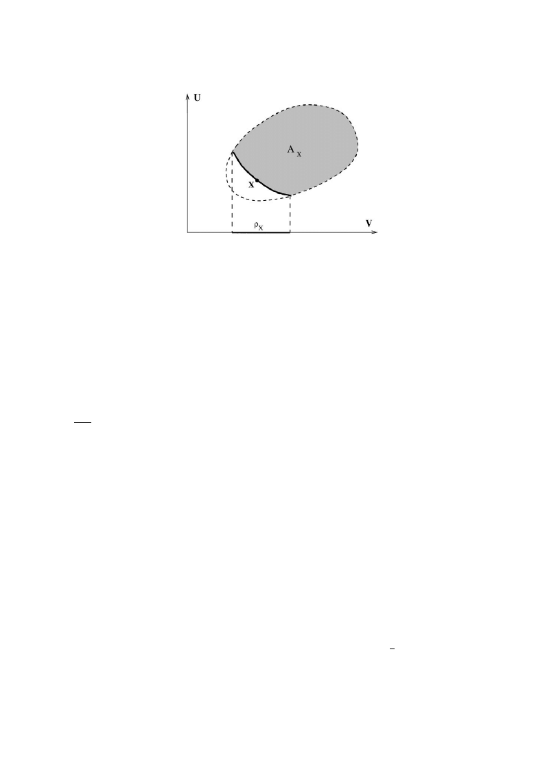
Fig. 4. This illustrates the energy º and work coordinates » of a simple system. The state space (dashed line) is always
a convex set and the forward sector A6 of any point X is always a convex subset of the state space. The heavy dark curve

denotes the boundary

jA6 of A6 and consists of points that are adiabatically equivalent to X (as Theorem 3.6 states). The

projection of this boundary on the work coordinates is

o6 which can be strictly smaller than the projection of A6.

he function u6 is continuous on o6 and locally convex, i.e., u6 is convex on any convex subset of o6.

(Note that

o6 need not be convex — or even contractible to a point.) Moreover,

A6M+(º, »): º5u6(»),»3o6,5C .

(3.16)

(iv) ¹he function u6 is a differentiable function on o6 with a locally ¸ipschitz continuous derivative

and satisfies the system of partial differential equations

ju6

j»H

(»)"!PH(u6(»),») for j"1,2,n .

(3.17)

(v) ¹he function u6 is the only continuous function defined on o6 that satisfies the differential

equation, (3.17), in the sense of distributions, and that satisfies u6(»)"º.

Remark. A solution to (3.17) is not guaranteed a priori; an integrability condition on P is needed.
However, our assumption S2 implies that P describes the boundary of A6 (cf. (i) above), so the

integrability condition is automatically fulfilled. Thus, a solution exists. It is the Lipschitz continu-
ity that yields uniqueness; indeed, it was precisely our desire to have a unique solution to (3.17) that
motivated axiom S2.

Proof. (i) Since ½3

jA6, A6 has some support plane, P, at ½. Since A6 is closed by Theorem 3.1 we

have ½3A6 and hence A7LA6 by transitivity, A2. Thus P also supports A7 at ½. By assumption

S2, A7 has a unique support plane at ½, namely P7. Therefore, P"P7.

(ii) Connectedness of

o6 follows immediately from assumption S3, i.e., jA6 is connected. The

following proof that

o6 is open does not use assumption S3. The key fact is that by (i) and S2 the

tangent plane to the convex set A6 has finite slope at any ½3jA6. Pick a ½"(º,»)3jA6. Since

C is open, the closed cylinder C"+(º, ») : "»!»"4e, "º!º"4(e, with ½ at its center lies
in

C for e'0 small enough. Since the tangent plane through ½ has finite slope, the bottom ‘disc’

E.H. Lieb, J. Yngvason / Physics Reports 310 (1999) 1—96

D\"+(º!(e, »): "»!»"(e, lies below the tangent plane for e small enough and thus

belongs to the complement of A6. Consider the intersection of A6 with the top disc,

D>"+(º#(e,»): "»!»"(e,. This intersection is compact, convex and contains the point

(º#

(e,») by Lemma 3.2 and A2 (the latter implies that A7LA6). Its boundary is also compact

and thus contains a point with minimal distance

d from the cylinder axis (i.e., from the point

(º#

(e, »)). We are obviously done if we show that d'0, for then all lines parallel to the cylinder

axis with distance (

d from the axis intersect both A6 and its complement, and hence the

boundary

jA6. Now, if d"0, it follows from Lemma 3.2 and transitivity that the vertical line

joining (º#

(e, ») and (º, ») has an empty intersection with the interior of A6. But then A6 has

a vertical support plane (because it is a convex set), contradicting S2.

(iii) The proof of Eqs. (3.14), (3.15) and (3.16) is already contained in Lemma 3.2, bearing in mind

that A7LA6 for all ½3jA6. The local convexity of u6 follows from its definition: Let CLo6 be

convex, let »

and » be in C and let 04j41. Then the point » :" j»#(1!j)» is in C

(by definition) and, by axiom A7, (

ju6(»)#(1!j)u6(»),») is in A6. Hence, by Eq. (3.15),

u6(»)4ju6(»)#(1!j)u6(»). Finally, every convex function defined on an open, convex subset

of R

L is continuous.

(iv) Fix »3

o6, let BLo6 be an open ball centered at » and let ½ :"(u6(»),»)3jA6. By (i)

above and Eq. (3.4) we have

u6(»)!u6(»)#

PG(½)(»G!»G)50

(3.18)

for all »

3B. Likewise, applying (i) above and Eq. (3.4) to the point ½ :"(u6(»),») we have

u6(»)!u6(»)#

PG(½)(»G!»G)50 .

(3.19)

As »

P», P(½)PP(½), since u6 is continuous and P is continuous. Thus, if 14j4n is fixed and

if »

G :"»G for iOj, »H"»H#e then, taking limits eP0 in the two inequalities above, we have

that

u6(»)!u6(»)

PH(½) ,

(3.20)

which is precisely (3.17).

By assumption P(½) is continuous, so u6 is continuously differentiable, and hence locally

Lipschitz continuous. But then P(u6(»),») is locally Lipschitz continuous in ».

(v) The uniqueness is a standard application of Banach’s contraction mapping principle, given

the important hypothesis that P is locally Lipschitz continuous and the connectedness of the open
set

o6. o6.

䊏

According to the last theorem the boundary of a forward sector is described by the unique

solution of a system of differential equations. As a corollary it follows that all points on the
boundary are adiabatically equivalent and thus have the same forward sectors:

Theorem 3.6 (Reversibility on the boundary). If ½3

jA6, then X3jA7 and hence A7"A6.

E.H. Lieb, J. Yngvason / Physics Reports 310 (1999) 1—96

Proof. Assume ½"(º

, »)3jA6. The boundary jA7 is described by the function u7 which solves

Eq. (3.17) with the condition u7(»)"º. But u6, which describes the boundary jA6, solves the

same equation with the same initial condition. This solution is unique on

o7 by Theorem 3.5(v), so we

conclude that

jA7LjA6 and hence o7Lo6. The theorem will be proved if we show that o6"o7.

Suppose, on the contrary, that

o7 is strictly smaller than o6. Then, since o6 is open, there is some

point »3

o6 that is in the boundary of o7, and hence »,o7 since o7 is open. We claim that jA7

is not relatively closed in

C, which is a contradiction since A7 must be relatively closed. To see

this, let »

H, for j"1, 2, 3,

2 be in

o7 and »HP» as jPR. Then u6(»H)Pu6(») since u6 is continu-

ous. But u7(»H)"u6(»H), so the sequence of points (u7(»H), ») in A6 converges to Z:"(u6(»), »)3C.

Thus, Z is in the relative closure of

jA7 but Z,jA7 because »,o7, thereby establishing

a contradiction.

䊏

We are now in a position to prove the main result in this section. It shows that

C is foliated by the

adiabatic surfaces

jA6, and that the points of C are all comparable. More precisely, XOO½ if and

only if A7 is contained in the interior of A6, and X

& ½

if and only if ½3

jA6.

Theorem 3.7 (Forward sectors are nested). ¼ith the above assumptions, i.e., A1—A7 and S1—S3, we
have the following. If A6 and A7 are two forward sectors in the state space, C, of a simple system then

exactly one of the following holds.

(a) A6"A7, i.e., X

& ½

(b) A6LInterior(A7), i.e., ½OOX.

In particular,

jA6 and jA7 are either identical or disjoint.

Proof. There are three (non-exclusive) cases:

Case 1. ½3A6

Case 2. X3A7

Case 3. X

,A7 and ½,A6.

By transitivity, case 1 is equivalent to A7LA6. Then, either ½3jA6 (in which case A7"A6 by

Theorem 3.6) or ½3Interior(A6). In the latter situation we conclude that jA7LInterior(A6), for

otherwise

jA75jA6 contains a point Z and Theorem 3.6 would tell us that jA7"jA8"jA6,

which would mean that A7"A6. Thus, case 1 agrees with the conclusion of our theorem.

Case 2 is identical to case 1, except for interchanging X and ½.
Therefore, we are left with the case that ½

,A6 and X,A7. This, we claim, is impossible for the

following reason.

Let Z be some point in the interior of A6 and consider the line segment ¸ joining ½ to Z (which

lies in

C since C is convex). If we assume ½,A6 then part of ¸ lies outside A6, and therefore

intersects

jA6 at some point ¼3jA6. By Theorem 3.6, A6 and A5 are the same set, so ¼OZ

(because X

OZ). By Lemma 3.1, ½OZ also. Since Z was arbitrary, we learn that Interior(A6)LA7.

By the same reasoning Interior(A7)LA6. Since A6 and A7 are both closed, the assumption that

,A6 and X,A7 has led us to the conclusion that they are identical.

䊏

Fig. 5 illustrates the content of Theorem 3.7. The end result is that the forward sectors are nicely

nested and thereby establishes the comparison hypothesis for simple systems, among other things.

E.H. Lieb, J. Yngvason / Physics Reports 310 (1999) 1—96

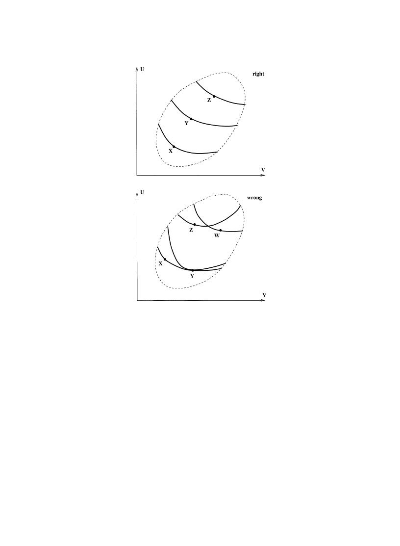
Fig. 5. The top figure illustrates how the forward sectors of a simple system are nested. The adiabats (i.e., the boundaries
of the forward sectors) do not overlap. The three points are related by X

OO½OOZ. The lower figure shows what, in

principle, could go wrong — but does not, according to Theorem 3.6. The top pair of adiabats have a point in common but
neither ¼

OZ nor ZO¼ holds. The bottom pair is a bit more subtle; XO½ and ½ is on the boundary of the forward

sector of X, but X is not in the forward sector of ½.

The adiabats

jA6 foliate C and using Theorem 3.5 it may be shown that there is always

a continuous function

p that has exactly these adiabats as level sets. (Such a function is usually

referred to as an ‘empirical entropy’.) But although the sets A6 are convex, the results established so

far do not suffice to show that there is a concave function with the adiabats as level sets. For this
and further properties of entropy we shall rely on the axioms about thermal equilibrium discussed in
the next section.

As a last topic in this section we would like to come back to the claim made in Section 2.1.2 that

our operational definition of the relation

O coincides with definitions in textbooks based on the

concept of ‘adiabatic process’, i.e., a process taking place in an ‘adiabatic enclosure’. We already
discussed the connection from a general point of view in Section 2.3, and showed that both
definitions coincide. However, there is also another point of view that relates the two, and which we

E.H. Lieb, J. Yngvason / Physics Reports 310 (1999) 1—96

now present. It is based on the idea that, quite generally, if one relation is included in another then
the two relations must coincide for simple systems. This very general result is Theorem 3.8 below.

Whatever ‘adiabatic process’ means, we consider it a minimal requirement that the relation

based on it is a subrelation of our

O, according to the operational definition in Section II.A. More

precisely, denoting this hypothetical relation based on ‘adiabatic process’ by

OH, it should be true

that X

OH½ implies XO½. Moreover, our motivations for the axioms A1—A6 and S1—S3 for

O apply equally well to OH, so we may assume that OH also satisfies these axioms. In particular,
the forward sector A

H6 of X with respect to OH is convex and closed with a nonempty interior and

with X on its boundary. The following simple result shows that

O and OH must then necessarily

coincide.

Theorem 3.8 (There are no proper inclusions). Suppose that

O and O are two relations on

multiple scaled products of a simple system

C satisfying axioms A1—A7 as well as S1—S3. If

O½ implies XO½

for all X,½3

C, then O"O.

Proof. We use superscripts (1) and (2) to denote the two cases. Clearly, the hypothesis is equivalent
to A

for all X3

C. We have to prove A

. Suppose not. Then there is a ½ such that

O½ but XO.½. By Theorem 3.7 for O we have that ½OX. By our hypothesis, ½OX,

and thus we have X

& ½

Now we use what we know about the forward sectors of simple systems. A

has a non-empty

interior, so the complement of A

in A

contains a point ½ that is not on the boundary of A

. On

the other hand, we just proved that X

& ½

, which implies that ½3

. This is a contradic-

tion.

䊏

4. Thermal equilibrium

In this section we introduce our axioms about thermal contact of simple systems. We then use

these assumptions to derive the comparison hypothesis for products of such systems. This will be
done in two steps. First we consider scaled copies of a single simple system and then products of
different systems. The key idea is that two simple systems in thermal equilibrium can be regarded as a
new simple system, to which Theorem 3.7 applies. We emphasize that the word ‘thermal’ has nothing
to do with temperature — at this point in the discussion. Temperature will be introduced in the next
section, and its existence will rely on the properties of thermal contact, but thermal equilibrium,
which is governed by the zeroth law, is only a statement about mutual equilibrium of systems and
not a statement about temperature.

4.1. Assumptions about thermal contact

We assume that a relation

O satisfying axioms A1—A6 is given, but A7 and CH are not assumed

here. We shall make five assumptions about thermal equilibrium, T1—T5. Our first axiom says that

E.H. Lieb, J. Yngvason / Physics Reports 310 (1999) 1—96

one can form new simple systems by bringing two simple systems into thermal equilibrium and that
this operation is adiabatic (for the compound system, not for each system individually).

(T1) Thermal contact. Given any two simple systems with state spaces

C and C, there is another

simple system, called the the thermal join of

C and C, whose state space is denoted by D.

The work coordinates in

D are (»,») with » the work coordinates of C and » the work

coordinates of

C. The range of the (single) energy coordinate of D is the sum of all possible

energies in

C and C for the given values of the work coordinates. In symbols:

D"+(º,»,»):º"º#º with (º,»)3C,(º,»)3C, .

(4.1)

By assumption, there is always an adiabatic process, called thermal equilibration that takes
a state in the compound system,

C;C, into a state in D which is given by the following

formula:

C;CU((º,»),(º,»))O(º#º,»,»)3D .

From the physical point of view, a state in

D is a ‘black box’ containing the two systems, with

energies º and º, respectively, such that º#º"º. The values of º and º need not be

unique, and we regard all such pairs (if there is more than one) as being equivalent since, by T2
below, they are adiabatically equivalent. This state in

D can be pictured, physically, as having the

two systems side by side (each with its own pistons, etc.) and linked by a copper thread that allows
‘heat’ to flow from one to the other until thermal equilibrium is attained. The total energy

º"º#º

can be selected at will (within the range permitted by » and »), but the individual

energies º and º will be determined by the properties of the two systems. Note that D is

convex — a fact that follows easily from the convexity of

C and C.

The next axiom simply declares the ‘obvious’ fact that we can disconnect the copper thread, once

equilibrium has been reached, and restore the original two systems.

(T2) Thermal splitting. For any point (º, », »)3D there is at least one pair of states,

(º, »)3C, (º, »)3C, with º"º#º, such that

DU(º,»,») & ((º,»),(º,»))3C;C .

In particular, the following is assumed to hold: If (º, ») is a state of a simple system

C and

j3[0, 1] then

(º,(1!

j)», j»)

(((1!

j)º, (1!j)»), (jº, j»))3C\H;CH .

We are now in a position to introduce another kind of equivalence relation among states, in

addition to

Definition. If ((º, »), (º,»))

(º#º, », ») we say that the states X"(º, ») and

½"

(º, ») are in thermal equilibrium and write

X 2

& ½

It is clear that X 2

& ½

implies ½ 2

X. Moreover, by axiom T2 and axioms A4 and A5 we always

have X 2

E.H. Lieb, J. Yngvason / Physics Reports 310 (1999) 1—96

The next axiom implies that 2

is, indeed, an equivalence relation. It is difficult to overstate its

importance since it is the key to eventually establishing the fact that entropy is additive not only with
respect to scaled copies of one system but also with respect to different kinds of systems.

(T3) Zeroth law of thermodynamics. If X 2

& ½

and if ½ 2

Z then X 2

The equivalence classes w.r.t. the relation 2

are called isotherms.

The question whether the zeroth law is really needed as an independent postulate or can be

derived from other assumptions is the subject of some controversy, see e.g., Buchdahl (1986),
Walter (1989), Buchdahl (1989). Buchdahl (1986) derives it from his analysis of the second law for
three systems in thermal equilibrium. However, it is not clear whether the zeroth law comes for free;
if we really pursued this idea in our framework we should probably find it necessary to invoke some
sort of assumption about the three-system equilibria.

Before proceeding further let us point out a simple consequences of T1—T3.

Theorem 4.1 (Scaling invariance of thermal equilibrium). If X and ½ are two states of two simple
systems (possibly the same or possibly different systems) and if

j, k'0 then the relation X 2

& ½

implies

jX 2

k½.

Proof. (X,

jX)"((º6,»6),(jº6,j»6)) & ((1#j)º6,»6,j»6) by axiom T2. But this means, by

the above definition of thermal equilibrium, that X 2

jX. In the same way, ½ 2

k½. By the zeroth

law, axiom T3, this implies

jX 2

k½.

䊏

Another simple consequence of the axioms for thermal contact concerns the orientation of

forward sectors with respect to the energy. In Theorem 3.3 in the previous section we had already
showed that in a simple system the forward sectors are either all on the positive energy side or all
on the negative energy side of the tangent planes to the sectors, but the possibility that the direction
is different for different systems was still open. The coexistence of systems belonging to both cases,
however, would violate our axioms T1 and T2. The different orientations of the sectors with respect
to the energy correspond to different signs for the temperature as defined in Section 5. Our axioms
are only compatible with systems of one sign.

Theorem 4.2 (Direction of forward sectors). ¹he forward sectors of all simple systems point the same
way, i.e., they are either all on the positive energy side of their tangent planes or all on the negative
energy side.

Proof. This follows directly from T1 and T2, because a system with sectors on the positive energy
side of the tangent planes can never come to thermal equilibrium with a system whose sectors are
on the negative side of the tangent planes. To be precise, suppose that

C has positive sectors,

C has negative sectors and that there are states X"(º,»)3C and ½"(º,»)3C such that

X 2

& ½

. (Such states exist by T2.) Then, for any sufficiently small

d'0,

(º, »)O(º#d, ») and (º, »)O(º!d, »)

E.H. Lieb, J. Yngvason / Physics Reports 310 (1999) 1—96

by Theorem 3.4 (Planck’s principle). With º :"º#º we then have the two relations

(º, », »)

((º,»), (º,»))O((º#d,»), (º,»))O(º#d,»,») ,

(º, »,»)

((º,»), (º,»))O((º,»), (º!d,»))O(º!d,»,») .

This means that starting from (º, »,»)3D we can move adiabatically both upwards and

downwards in energy (at fixed work coordinates), but this is impossible (by Theorem 3.3) because
D is a simple system, by axiom T1.

䊏

For the next theorem we recall that an entropy function on

C is a function that exactly

characterizes the relation

O on multiple scaled copies of C, in the sense of Theorem 2.2. As defined

in Section II, entropy functions S on C and S on C are said to be consistent if together they

characterize the relation

O on multiple scaled products of C and C in the sense of Theorem 2.5.

The comparison hypothesis guarantees the existence of such consistent entropy functions, by
Theorem 2.5, but our present goal is to derive the comparison hypothesis for compound systems by
using the notion of thermal equilibrium. In doing so, and also in Section 5, we shall make use of the
following consequence of consistent entropy functions.

Theorem 4.3 (Thermal equilibrium is characterized by maximum entropy). If S is an entropy function
on the state space of a simple system, then S is a concave function of º for fixed ». If S and S are

consistent entropy functions on the state spaces

C and C of two simple systems and (ºG,»G)3CG,

i"1, 2, then (º,») 2

(º,») holds if and only if the sum of the entropies takes its maximum value

at ((º,»), (º,»)) for fixed total energy and fixed work coordinates, i.e.,

max

[S(¼,»)#S((º#º)!¼),»)]"S(º,»)#S(º,») .

(4.2)

Proof. The concavity of S is true for any simple system by Theorem 2.8, which uses the convex
combination axiom A7. It is interesting to note, however, that concavity in º for fixed » follows
from axioms T1, T2 and A5 alone, even if A7 is not assumed. In fact, by axiom T1 we have, for states
(º, ») and (º

,») of a simple system with the same work coordinates,

(((1!

j)º, (1!j)»), (jº, j»))O((1!j)º#jº, (1!j)», j») .

By T2, and with º

:"(1!j)º#jº, this latter state is

equivalent to

((1!

j)º, (1!j)»), (jº, j») ,

which, by A5, is

equivalent to (º

,»). Since S is additive and non decreasing under O this

implies

(1!

j)S(º, »)#jS(º,»)4S((1!j)º#jº,») .

For the second part of our theorem, let (º,») and (º,») be states of two simple systems.

Then T1 says that for any ¼ such that (¼,»)3C and ((º#º!¼),»)3C one has

((¼,»), ((º#º)!¼),»))O(º#º,»,») .

E.H. Lieb, J. Yngvason / Physics Reports 310 (1999) 1—96

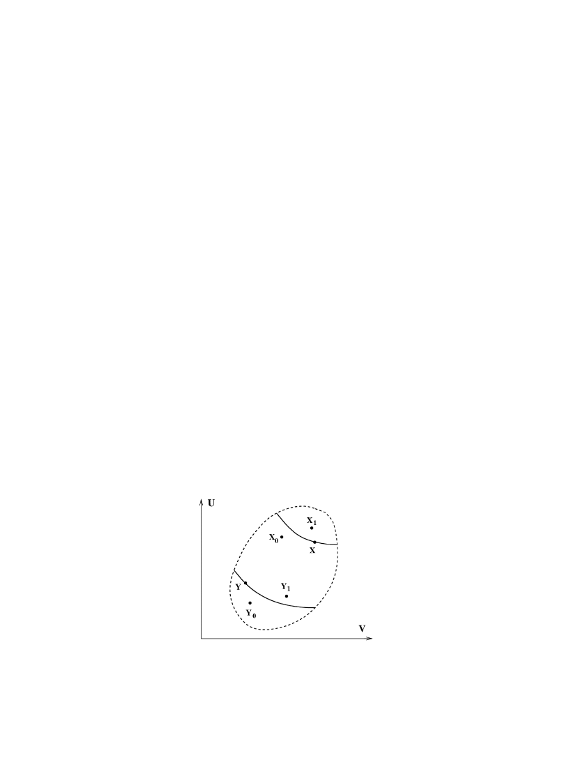
Fig. 6. This illustrates the transversality axiom T4. For every state X there are points X and X on both sides of the

adiabat through X that are in thermal equilibrium with each other. The points ½ and ½ (corresponding to some other

point ½) need not be in thermal equilibrium with X and X.

The definition of thermal equilibrium says that (º#º,»,»)

((º,»)(º,»)) if and only if

(º,») 2

(º,»). Since the sum of consistent entropies characterizes the order relation on the

product space the assertion of the lemma follows.

䊏

We come now to what we call the transversality axiom, which is crucial for establishing the

comparison hypothesis, CH, for products of simple systems.

(T4) Transversality. If

C is the state space of a simple system and if X3C, then there exist states

X 2

X with XOOXOOX.

To put this in words, the axiom requires that for every adiabat there exists at least one isotherm

(i.e., an equivalence class w.r.t. 2

), containing points on both sides of the adiabat. Note that, for

each given X, only two points in the entire state space

C are required to have the stated property.

See Fig. 6.

We remark that the condition X

OOX obviously implies axiom S1. However, as far as the

needs of this Section 4 are concerned, the weaker condition XOXOX together with XOOX

would suffice, and this would not imply S1. The strong version of transversality, stated above, will
be needed in Section 5, however.

At the end of this section we shall illustrate, by the example of ‘thermometers’, the significance of

axiom T4 for the existence of an entropy function. There we shall also show how an entropy
function can be defined for a system that violates T4, provided its thermal combination with some
other system (that itself satisfies T4) does satisfy T4.

The final thermal axiom states, essentially, that the range of temperatures that a simple system

can have is the same for all simple systems under consideration and is independent of the work
coordinates. In this section axiom T5 will be needed only for Theorem 4.9. It will also be used again
in the next section when we establish the existence and properties of temperature. (We repeat that
the word ‘temperature’ is used in this section solely as a mnemonic.)

E.H. Lieb, J. Yngvason / Physics Reports 310 (1999) 1—96

(T5) Universal temperature range. If

C and C are state spaces of simple systems then, for every

C and every »3o(C), where o denotes the projection on the work coordinates,

o(º,») :"», there is a ½3C with o(½)"», such that X 2& ½.

The physical motivation for T5 is the following. A sufficiently large copy of the first system in the

state X3

C can act as a heat bath for the second, i.e., when the second system is brought into

thermal contact with the first at fixed work coordinates, », it is always possible to reach thermal
equilibrium, but the change of X will be very small since X is so large.

This axiom is inserted mainly for convenience and one might weaken it and require it to

hold only within a group of systems that can be placed in thermal contact with each other.
However, within such a group this axiom is really necessary if one wants to have a consistent
theory.

4.2. The comparison principle in compound systems

4.2.1. Scaled copies of a single simple system

We shall now apply the thermal axioms, T4 in particular, to derive the comparison hypothesis,

CH, for multiple scaled copies of simple systems.

Theorem 4.4 (Comparison in multiple scaled copies of a simple system). ¸et

C be the state space

of a simple system and let a,2, a+, a,2, a+ be positive real numbers with a#2#a,"

#2#a+. ¹hen all points in aC;2;a,C are comparable to all points in aC;2;a+C.

Proof. We may suppose that a#2#a,"a#2#a+"1. We shall show that for

any

points

½,2,½,, ½,2,½+3C there exist points

XOOX in C such that

(a½,2, a,½,)

((1!

a)X,aX) and (a½,2,a,½,) & ((1!a)X,aX) with a,a3R. This

will prove the statement because of Lemma 2.2.

By Theorem 3.7, the points in

C are comparable, and hence there are points XOX such that all

the points ½,2,½,,½,2,½+ are contained in the strip R(X, X)"+X3C: XOXOX,; in

particular, these N#M points can be linearly ordered and X and X can be chosen from this set.

If X

X then all the points in the strip would be equivalent and the assertion would hold

trivially. Hence we may assume that XOOX. Moreover, it is clearly sufficient to prove that for

each ½3

R(X,X) one has ½ & ((1!j)X,jX) for some j3[0,1], because the general case then

follows by the splitting and recombination axiom A5 and Lemma 2.2.

If X 2

X (or, if there exist X

X and X

X with X 2

, which is just as good for

the present purpose) the existence of such a

j for a given ½ can be seen as follows. For any j3[0, 1]

the states ((1!

j)X,jX) and ((1!j)½,j½) are adiabatically equivalent to certain states in the

state space of a simple system, thanks to thermal axiom T2. Hence ((1!

j)X,jX) and

((1!

j)½, j½) are comparable. We define

j"sup+j3[0, 1]: ((1!j)X,jX)O½, .

(4.3)

Since XO½ the set on the right of (4.3) is not empty (it contains 0) and therefore j is well defined

and 04

j41. Next, one shows that ((1!j)X,jX) & ½ by exactly the same argument as in

E.H. Lieb, J. Yngvason / Physics Reports 310 (1999) 1—96

Lemma 2.3. (Note that this argument only uses that ½ and ((1!

j)X,jX) are comparable.) Thus,

our theorem is established under the hypothesis that X 2

The following Lemma 4.1 will be needed to show that we can, indeed, always choose X and

X so that X 2

Lemma 4.1 (Extension of strips). For any state space (of a simple or a compound system), if
XOOX, XOOX and if

((1!

j)X,jX) ,

(4.4)

((1!

j)X,jX) ,

(4.5)

& ((1!j)X,jX) ,

(4.6)

then

((1!

k)X,kX)

(4.7)

with

j#jj

Proof. We first consider the special case X"X, i.e., j"1. By simple arithmetic, using the

cancellation law, one obtains (4.7) from (4.5) and (4.6) with

k"k"j/(1!j#jj). The

general case now follows by inserting the splitting of X into (4.4) and recombining. 䊐

Proof of Theorem 4.4 (continued). By the transversality property, each point X lies in some strip
R(X,X) with XOOX and X 2& X. Hence the whole state space can be covered by strips

, X

) with X

and X

. Here i belongs to some index set. Since all adiabats

jA6 with X3C are relatively closed in C by axiom S3 we can even cover each X (and hence C) with

open strips

M(XG,XG)"+X:XGOOXOOXG, with XG 2& XG. Moreover, any compact

subset, C, of

C is covered by a finite number of such strips

, i"1,2, K, and if C is connected

we may assume that

. If XM denotes the smallest of the elements XG (with respect to

the relation

O) and XM the largest, it follows from Lemma 2.3 that for any X3C we have

((1!

k)XM,kXM) for some k. If a finite number of points, ½,2,½,,½,2,½+ is given, we

take C to be a polygon connecting the points, which exists because

C is convex. Hence each of

the points ½,2,½,,½,2,½+ is equivalent to ((1!j)XM, jXM) for some j, and the proof is

complete.

䊏

The comparison hypothesis, CH, has thus been established for multiple scaled copies of

a single simple system. From Theorem 2.2 we then know that for such a system the rela-
tion

O is characterized by an entropy function, which is unique up to an affine transformation

SPaS#B.

E.H. Lieb, J. Yngvason / Physics Reports 310 (1999) 1—96

4.2.2. Products of different simple systems

Our next goal is to verify the comparison hypothesis for products of different simple systems. For

this task we shall appeal to the following:

Theorem 4.5 (Criterion for comparison in product spaces). ¸et

C and C be two (possibly unrelated)

state spaces. Assume there is a relation

Osatisfying axioms A1—A6 that holds for C,C and their

scaled products. Additionally,

O satisfies the comparison hypothesis CH on C and its multiple scaled

copies and on

C and its multiple scaled copies but, a priori, not necessarily on C;C or any other

products involving both

C and C

If there are points X, X3C and ½,½3C such that

XOOX, ½OO½ ,

(4.8)

(X,½)

(X,½) ,

(4.9)

then the comparison hypothesis CH holds on products of any number of scaled copies of

C and C.

Proof. Since the comparison principle holds for

C and C these spaces have canonical entropy

functions corresponding, respectively, to the reference points X, X and ½,½. If X3C and

j"S(X"X,X) (in the notation of Eq. (2.15)) then, by Lemma 2.3,

((1!

j)X,jX)

and similarly, for ½3

C and j"S(½"½,½),

((1!

j)½,j½) .

Set

j"(j#j) and d"(j!j). We then have

(X,½)

((1!

j)X,jX,(1!j)½,j½)

by A3

((1!

j)X,!dX,jX,dX,1!j)½,d½,j½,!d½) by A5

((1!

j)X,!dX,jX,dX,(1!j)½,d½,j½,!d½) by Eq. (4.9), A3, A4

((1!

j)(X,½),j(X,½))

by A5 .

Thus, every point in

C;C":C is equivalent to a point of the form ((1!j)Z,jZ) in

(1!

j)C;jC with Z"(X,½) and Z"(X,½) fixed and j3R. But any two points of this

form (with the same Z,Z, but variable j) are comparable by Lemma 2.2.

A similar argument extends CH to multiple scaled copies of

C. Finally, by induction, CH

extends to scaled products of

C and C and C, i.e., to scaled products of arbitrarily many copies

C and C.

䊏

We shall refer to a quadruple of points satisfying Eqs. (4.8) and (4.9) as an entropy calibrator. To

establish the existence of such calibrators we need the following result.

E.H. Lieb, J. Yngvason / Physics Reports 310 (1999) 1—96

Theorem 4.6 (Transversality and location of isotherms). ¸et

C be the state space of a simple system

that satisfies the thermal axioms ¹1—¹4. ¹hen either

(i) All points in

C are in thermal equilibrium, i.e., X 2

& ½

for all X,½3

(ii) ¹here is at least one adiabat in

C (i.e., at least one jA6) that has at least two points that are not in

thermal equilibrium, i.e., Z 2

& ½

is false for some pair of points Z and ½ in

jA6.

Proof. Our proof will be somewhat indirect because it will use the fact — which we already
proved — that there is a concave entropy function, S, on

C which satisfies the maximum principle,

Theorem 4.3 (for

C"C"C). This means that if RLR denotes the range of S on C then the sets

EN"+X3C: S(X)"p,, p3R

are precisely the adiabats of

C and, moreover, X"(º,»), ½"(º,») in C satisfy X 2& ½ if and

only if ¼"º, maximizes S(º#º!¼,»)#S(¼,») over all choices of ¼ such that

(º#º!¼,»)3C and (¼,»)3C. Furthermore, the concavity of S — and hence its continuity

on the connected open set

C — implies that R is connected, i.e., R is an interval.

Let us assume now that (ii) is false. By the zeroth law, T3, 2

is an equivalence relation that

divides

C into disjoint equivalence classes. Since (ii) is false, each such equivalence class must be

a union of adiabats, which means that the equivalence classes are represented by a family of disjoint
subsets of R. Thus

R? ,

where I is some index set, R? is a subset of R, R?5R@"0 for aOb, and EN 2

EO if and only if

p and q are in some common R?.

We will now prove that each R? is an open set. It is then an elementary topological fact (using the

connectedness of

C) that there can be only one non-empty R?, i.e., (i) holds, and our proof is

complete.

The concavity of S(º, ») with respect to º for each fixed » implies the existence of an upper and

lower º-derivative at each point, which we denote by 1/¹> and 1/¹\, i.e.,

(1/¹!)(º,»)"$lim

e\[S(º$e,»)!S(º, »)] .

Theorem 4.3 implies that X 2

& ½

if and only if the closed intervals [¹\(X),¹>(X)] and

[¹\(½),¹>(½)] are not disjoint. Suppose that some R? is not open, i.e., there is p3R? and either

a sequence

p'p'p2, converging to p or a sequence p(p(p(2 converging to

p with pG,R?. Suppose the former (the other case is similar). Then (since ¹! are monotone

increasing in º by the concavity of S) we can conclude that for every ½3EN

and every X3EN

¹\

(½)'¹>(X) .

(4.10)

E.H. Lieb, J. Yngvason / Physics Reports 310 (1999) 1—96

We also note, by the monotonicity of ¹! in º, that (4.10) necessarily holds if ½3EI and k5pG;

hence (1) holds for all ½3EI for any k'p (because pGWp). On the other hand, if q4p

¹>

(Z)4¹\(X)

for Z3EO and X3EN. This contradicts transversality, namely the hypothesis that there is q(p(k,

Z3EO,½3EI such that [¹\(Z),¹>(Z)]5[¹\(½),¹>(½)] is not empty.

䊏

Theorem 4.7 (Existence of calibrators). ¸et

C and C be state spaces of simple systems and assume

the thermal axioms, ¹1—¹4, in particular the transversality property ¹4. ¹hen there exist states
X, X3C and ½,½3C such that

XOOX and ½OO½ ,

(4.11)

(X,½)

(X,½) .

(4.12)

Proof. Consider the simple system

D obtained by thermally coupling C and C. Fix some

M "(º6

,»6

C and ½M"(º7

,»7

C with XM 2& ½M. We form the combined state

(XM,½M)"(º6

#º7

,»6

,»7

D and consider the adiabat jA

(

D. By axiom T2 every

point Z3

(

can be split in at least one way as

t(Z)"((º6,»6),(º7,»7))3C;C ,

(4.13)

where (»6,»7) are the work coordinates of Z with º6#º7"º8 and where X"(º6,»6),

½"

(º7,»7) are in thermal equilibrium, i.e., X 2

& ½

. If the splitting in (4.13) is not unique, i.e., there

exist X

,½ and X,½ satisfying these conditions, then we are done for the following reason:

First, (X

,½)

,½) (by axiom T2). Second, since º6

#º7

"º6

#º7

we have

either º6

(º6

, º7

'º7

or º6

'º6

,º7

(º7

. This implies, by Theorem 3.4, that

either X

OOX and ½OO½ or XOOX and ½OO½.

Let us assume, therefore, that the thermal splitting (4.13) of each Z3

(

is unique so we can

write

t(Z)"(X,½) with uniquely determined X 2

& ½

. (This means, in particular, that alternative (i)

in Theorem 4.6 is excluded.) If some pair (X,½) obtained in this way does not satisfy X

M and

& ½

M , e.g., XOOXM holds, then it follows from axiom A3 and the cancellation law that ½MOO½,

and thus we have obtained points with the desired properties.

So let us suppose that X

M and ½

& ½

M whenever (X,½)"t(Z) and Z3jA

(

. In other

words,

t(jA

(

jA6

;jA7

. We then claim that all Z3

(

are in thermal equilibrium with

each other. By the zeroth law, T3, (and since

o(jA

(

) is open and connected, by the definition of

a simple systems) it suffices to show that all points (º, »,») in jA

(

with » fixed are in

thermal equilibrium with each other and, likewise, all points (º, »,») in jA

(

with » fixed are

in thermal equilibrium with each other. Now each fixed » in o(A6

) determines a unique point

(º,»)3jA6

(by Theorem 3.5 (iii)). Since, by assumption,

t(º, »,»)LjA6

;jA7

we must then

have

t(º, »,»)"((º,»)),(º,»))

(4.14)

with º"º!º. But (4.14), together with the zeroth law, implies that all points

(º, »,»)3jA

(

with » fixed are in thermal equilibrium with (º,») (because (4.14)

E.H. Lieb, J. Yngvason / Physics Reports 310 (1999) 1—96

shows that they all have the same

C component) and hence they are in thermal equilibrium

with each other. The same argument shows that all points with fixed » are in thermal

equilibrium.

We have demonstrated that the hypothesis X

M and ½

& ½

M for all (X,½)3t(jA

(

) implies

that all points in

(

are in thermal equilibrium. Since, by Theorem 4.6, at least one adiabat in

D contains at least two points not in thermal equilibrium, the existence of points satisfying (1) and

(2) is established.

䊏

Having established the entropy calibrators we may now appeal to Theorem 4.5 and summarize

the discussion so far in the following theorem.

Theorem 4.8 (Entropy principle in products of simple systems). Assume axioms A1—A7, S1—S3 and

1— ¹4. ¹hen the comparison hypothesis CH is valid in arbitrary scaled products of simple systems.

Hence, by ¹heorem 2.5, the relation

Oamong states in such state spaces is characterized by an entropy

function S. ¹he entropy function is unique, up to an overall multiplicative constant and one additive
constant for each simple system under consideration.

4.3. The role of transversality

It is conceptually important to give an example of a state space

C of a simple system and

a relation

O on its multiple scaled copies, so that all our axioms except ¹4 are satisfied. In this

example the comparison hypothesis CH is violated for the spaces

C;C and hence the relation can

not be characterized by an entropy function. This shows that the transversality axiom T4 is
essential for the proof of Theorem 4.8. The example we give is not entirely academic; it is based on
the physics of thermometers. See the discussion in the beginning of Section 3.1.

For simplicity, we choose our system to be a degenerate simple system, i.e., its state space is

one-dimensional. (It can be interpreted as a system with a work coordinate » in a trivial way, by
simply declaring that everything is independent of » and the pressure function is identically zero).
A hypothetical universe consisting only of scaled copies of such a system (in addition to mechanical
devices) might be referred to as a ‘world of thermometers’. The relation

O is generated, physically

speaking, by two operations: ‘rubbing’, which increases the energy, and thermal equilibration of
two scaled copies of the system.

To describe this in a more formal way we take as our state space

C"R>"+º:º'0,.

Rubbing the system increases º and we accordingly define

O on C simply by the relation 4 on

the real numbers º. On

;CH

we define the forward sector of (jº,jº) as the convex hull

of the union A

6B of two sets of points,

+(jº,jº): º4º, º4º, ,

+(jº,jº): ºM4º,ºM4º,

with

M "(j#j)\(jº#jº) .

E.H. Lieb, J. Yngvason / Physics Reports 310 (1999) 1—96

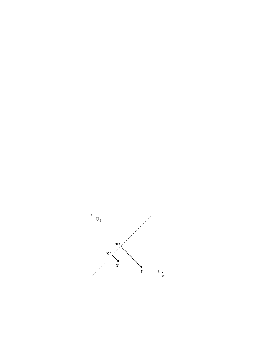
Fig. 7. This shows the state space of two ‘thermometers’, which means that there are only energy coordinates. The
forward sectors of X and ½ are shown under the assumption that the only allowed adiabatic operations are thermal
equilibration (which moves X to X

and ½ to ½) and rubbing (which increases, but never decreases the energy). We see

clearly that these sectors are not nested (i.e., one does not lie inside the other), as they are for compounds of simple
systems, satisfying the transversality axiom T4.

This choice of forward sector is minimally consistent with our axioms. The set A corresponds to
rubbing the individual thermometers while B corresponds to thermal equilibration followed by
rubbing.

The forward sector of a point (

jº,2,jLºL) in the product of more than two scaled copies of

C is then defined as the convex hull of all points of the form

(

jº,2,jGºG,2jHºH,2jLºL) with (jGºG,jHºH)O(jGºG,jHºH) .

The thermal join of

and CH

is identified with CH

. Thermal equilibration is simply

addition of the energies, and

jº is in thermal equilibrium with jº if and only if º"º.

Since the adiabats and isotherms in

C coincide (both consist only of single points) axiom T4 is

violated in this example. The forward sectors in

C;C are shown in Fig. 7. It is evident that these

sectors are not nested and hence cannot be characterized by an entropy function. This example thus
illustrates how violation of the transversality axiom T4 can prevent the existence of an entropy
function for a relation

O that is well behaved in other ways.

On the other hand we may recall the usual entropy function for a body with constant heat

capacity, namely

S(º)"ln º .

(4.15)

In the above example this function defines, by simple addition of entropies in the obvious way,
another relation,

OH, on the multiple scaled copies of C which extends the relation O previously

defined. On

C the two relations coincide (since S is a monotonous function of º), but on C;C this

is no longer the case: The inequality S(º)#S(º)4S(º)#S(º), i.e., ºº4ºº, is only

a necessary but not a sufficient condition for (º, º)O(º, º) to hold. The passage from (º, º)

to (º

,º) in the sense of the relation OH (but not O) may, however, be accomplished by coupling

each copy of

C to another system, e.g., to a Carnot machine that uses the two copies of C as heat

E.H. Lieb, J. Yngvason / Physics Reports 310 (1999) 1—96

reservoirs. From the relation

OH one could then reconstruct S in Eq. (4.15) by the method of

Section 2. The lesson drawn is that even if T4 fails to hold for a system, it may be possible to
construct an entropy function for that system, provided its thermal join with some other system
behaves normally.

A precise version of this idea is given in the following theorem.

Theorem 4.9 (Entropy without transversality). Suppose

C and C are normal or degenerate simple

systems and assume that axioms A1—A5, ¹1—¹3 and ¹5 hold for the relation

O on scaled products of

C and C. (¹hey already hold for C and C separately — by definition.) ¸et D be the thermal join of

C and C and suppose that D and C have consistent entropy functions S and S, which holds, in

particular, if ¹4 is valid for

D and C. ¹hen C has an entropy function S that is consistent with S

and satisfies

S((X,½))"S(X)#S(½)

if X 2

& ½

, where

is the canonical map C;CPD, given by (X,½)"(º6#º7,»6,»7) if

X"(º6,»6) and ½"(º7,»7).

Proof. Given X3

C we can, by axiom T5, find a ½3C with X 2& ½, and hence

Z :"

(X,½)

(X,½) by axiom T2. If ½

3C is another point with X 2& ½ and Z:"(X,½) then,

by axiom T2, (½

, Z)

(½

, X,½)

(½, (X,½

))

(½, Z

). Since S and S are consistent entropies,

this means that

S(½)#S(Z)"S(½)#S(Z) ,

S(Z)!S(½)"S(Z)!S(½) .

(4.16)

We can thus define S on C by

S(X):"S((X,½))!S(½)

(4.17)

for each X3

C and for any ½ satisfying ½ 2

X, because, according to (4.16), the right-hand side of

Eq. (4.17) is independent of ½, as long as ½ 2

To check that S is an entropy on C we show first that the relation

(X, X)O(X, X)

with X, X, X, X3C is equivalent to

S(X)#S(X)4S(X)#S(X) .

(4.18)

We pick ½,½,½,½3C with ½ 2

X,½ 2

X, etc. and insert the definition (4.17) of S into

Eq. (4.18). We then see that Eq. (4.16) is equivalent to

S((X,½))#S(½)#S((X,½))#S(½)

S((X,½))#S(½)#S((X,½))#S(½) .

E.H. Lieb, J. Yngvason / Physics Reports 310 (1999) 1—96

Since S and S are consistent entropies, this is equivalent to

(

(X,½),½,(X,½),½)O((X,½),½,(X,½),½) .

By the splitting axiom T2 this is equivalent to

(X,½,½, X,½,½)O(X,½,½, X,½,½) .

The cancellation law then tells us that this holds if and only if (X,X)O(X, X).

To verify more generally that S characterizes the relation on all multiple scaled copies of C one

may proceed in exactly the same way, using the scale invariance of thermal equilibrium (Theorem
4.1) and the hypothesis that S and S are entropy functions, which means that they characterize

the relation on all products of scaled copies of

D and C.

䊏

5. Temperature and its properties

Up to now we have succeeded in proving the existence of entropy functions that do everything

they should do, namely specify exactly the adiabatic processes that can occur among systems, both
simple and compound. The thermal join was needed in order to relate different systems, or copies of
the same system to each other, but temperature, as a numerical quantifier of thermal equilibrium,
was never used. Not even the concept of ‘hot and cold’ was used. In the present section we shall
define temperature and show that it has all the properties it is normally expected to have.
Temperature, then, is a corollary of entropy; it is epilogue rather than prologue.

One of our main results here is equation (5.3): Thermal equilibrium and equality of temperature

are the same thing. Another one is Theorem 5.3 which gives the differentiability of the entropy and
which leads to Maxwell’s equations and other manipulations of derivatives that are to be found in
the usual textbook treatment of thermodynamics.

Temperature will be defined only for simple systems (because 1/(temperature) is the variable dual

to energy and it is only the simple systems that have only one energy variable).

5.1. Differentiability of entropy and the existence of temperature

The entropy function, S, defined on the (open, convex) state space,

C, of a simple system is

concave (Theorem 2.8). Therefore (as already mentioned in the proof of Theorem 4.5) the upper and
lower partial derivatives of S with respect to º (and also with respect to ») exist at every point
X3

C, i.e., the limits

1/¹>(X)"lim

[S(º#

e,»)!S(º, »)] ,

1/¹\(X)"lim

[S(º, »)!S(º!

e,»)]

exist for every X"(º, »)3

C. The functions ¹>(X) (resp. ¹\(X)) are finite and positive everywhere

(since S is strictly monotone increasing in º for each fixed » (by Planck’s principle, Theorem 3.4).

E.H. Lieb, J. Yngvason / Physics Reports 310 (1999) 1—96

These functions are called, respectively, the upper and lower temperatures. Evidently, concavity
implies that if º(º

¹\(º,»)4¹>(º,»)4¹\(º,»)4¹>(º,»)

(5.1)

for all ». The concavity of S alone does not imply continuity of these functions. Our goal here is to
prove continuity by invoking some of our earlier axioms.

First, we prove a limited kind of continuity.

Lemma 5.1 (Continuity of upper and lower temperatures on adiabats). ¹he temperatures ¹> and

¹\

are locally ¸ipschitz continuous along each adiabat

jA6. I.e., for each X3C and each closed ball

B6 PLC of radius r and centered at X there is a constant c(X,r) such that

"¹>(X)!¹>(½)"4c(X,r)"X!½"

for all ½3

jA6 with "X!½"(r. ¹he same inequality holds for ¹\(X). Furthermore, c(X,r) is

a continuous function of X in any domain DL

C such that B6PLC for all X3D.

Proof. Recall that the pressure P(X) is assumed to be locally Lipschitz continuous and that
jº/j»G"PG on adiabats. Write X"(º,») and let the adiabatic surface through X be denoted

by (¼(»),») where ¼(») is the unique solution to the system of equations

j¼(»)

j»G

PG(¼(»),»)

with ¼(»)"º. (Thus ¼ is the function u6 of Theorem 3.5.) Similarly, for e'0 we let ¼C(»)

be the solution to

j¼C (»)

j»G

PG(¼C(»),»)

with ¼C(»)"º#e. Of course all this makes sense only if "»!»" and e are sufficiently small so

that the points (¼C(»),») lie in C. In this region (which we can take to be bounded) we let C denote

the Lipschitz constant for P, i.e.

"P(Z)!P(Z)"4C"Z!Z" for all Z, Z in the region.

Let SC denote the entropy on (¼C(»),»); it is constant on this surface by assumption. By

definition

¹>

(º,»)

lim

SC!S

¹>(¼(»), »)"lim

¼C

(»)!¼(»)

SC!S

"¹>(º, »)

lim

GC(»)#1

where GC(») :"C[¼C(»)!¼(»)!e]. The lemma will be proved if we can show that there is

a number D and a radius R'0 such that GC(»)4D"»!»" for all "»!»"(R.

Let v be a unit vector in the direction of »!» and set »(t)"»#tv, so that

(0)"», »(t)"» for t""»!»". Set ¼C(t) :"¼C(»(t)) and P(º,t) :"v) P(º, »(t)). Fix ¹'0

E.H. Lieb, J. Yngvason / Physics Reports 310 (1999) 1—96

so that C¹4

and so that the ball B62 with center X and radius 2¹ satisfies B62LC. Then, for

04t4¹ and

e small enough

(t)"º#

P(¼(t),t)dt ,

¼C

(t)!

e"º#

P(¼C(t)!e#e,t)dt .

Define

gC" sup

XRX2

[¼C(t)!e!¼(t)]" sup

XRX2

GC(»(t)) .

By subtracting the equation for ¼ from that of ¼C we have that

"GC(»(t))"4

C[1#gC]dt4tC[1#gC] .

By taking the supremum of the left side over 04t4¹ we obtain gC4¹C[1#gC], from which we

see that gC41 (because ¹C4). But then "GC(»(t)"42tC or, in other words, "GC(»)"42"»!»"C

whenever

"»!»"(¹, which was to be proved.

䊏

Before addressing our next goal — the equality of ¹> and ¹\ — let us note the maximum entropy

principle, Theorem 4.2, and its relation to ¹!. The principle states that if X"(º,») and

X"(º,») are in C then X 2

X if and only if the following is true:

S(X)#S(X)"sup

+S(º#º!¼,»)#S(¼,»):(º#º!¼,»)3C

and (¼,»)3C, .

(5.2)

Since S is concave, at every point X3

C there is an upper temperature and lower temperature, as

given in (5.1). This gives us an ‘interval-valued’ function on

C which assigns to each X the interval

(X)"[¹\(X), ¹>(X)] .

If S is differentiable at X then ¹\(X)"¹>(X) and the closed interval ¹(X) is then merely the

single number (

jS/jº)(X). If ¹\(X)"¹>(X) we shall abuse the notation slightly by thinking of

(X) as a number, i.e., ¹(X)"¹\(X)"¹>(X).

The significance of the interval ¹(X) is that Eq. (5.2) is equivalent to

X 2

X if and only if ¹(X)5¹(X)O .

In other words, if

jS/jº makes a jump at X then one should think of X as having all the

temperatures in the closed interval ¹(X).

In Theorem 5.1 we shall prove that the temperature is single-valued, i.e., ¹\(X)"¹>(X). Thus,

we have the following fact relating thermal equilibrium and temperature:

X 2

X if and only if ¹(X)"¹(X) .

(5.3)

E.H. Lieb, J. Yngvason / Physics Reports 310 (1999) 1—96

Theorem 5.1 (Uniqueness of temperature). At every point X in the state space of a simple system,

we have

¹>

(X)"¹\(X) ,

i.e., ¹(X) is the number [(

jS/jº)(X)]\.

Proof. The proof will rely heavily on the zeroth law, on the continuity of ¹! on adiabats, on

transversality, on axiom T5 and on the maximum entropy principle for thermal equilibrium,
Theorem 4.2.

Assume that Z3

C is a point for which ¹>(Z)'¹\(Z). We shall obtain a contradiction from

this.

Part 1: We claim that for every ½3

jA8, ¹>(½)"¹>(Z) and ¹\(½)"¹\(Z). To this end define

the (conceivably empty) set KL

C by K"+X3C : ¹>(X)"¹\(X)3¹(Z),. If X3K and X3K

then ¹(X)"¹(X)3¹(Z) by the zeroth law (since X 2

Z and X 2

Z, and thus X 2

X).

Therefore, there is a single number ¹

H3¹(Z) such that ¹(X)"¹H for all X3K.

Now suppose that ½3

jA8 and that ¹>(½)(¹>(Z). By the continuity of ¹> on jA8 (Lemma

5.1) there is then another point ¼3

jA8 such that ¹\(Z)4¹>(¼)(¹>(Z), which implies that

Z. We write ¼"(º5,»5) and consider f5(º)"S(º,»5), which is a concave function of

one variable (namely º) defined on some open interval containing º5. It is a general fact about

concave functions that the set of points at which f5 is differentiable (i.e., ¹>"¹\) is dense and

that if º'º'º'2'º5 is a decreasing sequence of such points converging to º5 then

(ºG) converges to ¹>(º5). We denote the corresponding points (ºG,»5) by ¼G and note that, for

large i, ¹(¼G)3¹(Z). Therefore ¹(¼G)"¹H for all large i and hence ¹>(¼)"¹H.

Now use continuity again to find a point R3

jA8 such that ¹H"¹>(¼)(¹>(R)(¹>(Z).

Again there is a sequence RG"(ºG,»0) with ¹>(RG)"¹\(RG)"¹(RG) converging downward to

R and such that ¹(RG)P¹>(R)'¹H. But for large i, ¹(RG)3¹(Z) so ¹(RG)"¹H. This is a contra-

diction, and we thus conclude that

¹>(½)"¹>(

for all ½3

jA8 when ¹>(Z)'¹\(Z).

Likewise ¹\(½)"¹\(Z) under the same conditions.

Part 2: Now we study

o8LRL, which is the projection of jA8 on RL. By Theorem 3.3, o8 is open

and connected. It is necessary to consider two cases.

Case 1:

o8 is the projection of C, i.e., o8"+»3RL:(º,»)3C for some º3R,"o(C). In this case

we use the transversality axiom T4, according to which there are points X and ½ in

C with

OOZOO½, (and hence S(X)(S(Z)(S(½)), but with X 2

& ½

. We claim that every X with

S(X)(S(Z)

has

¹>

(X)4¹\(Z). Likewise, we claim that S(½)'S(Z) implies that

¹\(½)5¹>(

Z). These two facts will contradict the assumption that ¹(½)

5¹(X) is not empty. To

prove that ¹>(X)4¹\(Z) we consider the line (º, »6)5C. As º increases from the value º6, the

temperature ¹>(º, »6) also cannot decrease (by the concavity of S). Furthermore,

(º6,»6)O(º, »6) if and only if º5º6 by Theorem 3.4. Since o8"o(C) there is (by Theorem 3.4)

some º'º6 such that (º,»6)3jA8. But ¹\(º,»6)"¹\(Z) as we proved above. However,

¹>

(X)4¹\(º,»6) by (5.1). A similar proof shows that ¹\(½)5¹>(Z) when S(½)'S(Z).

E.H. Lieb, J. Yngvason / Physics Reports 310 (1999) 1—96

Case 2:

o8Oo(C). Here we use T5. Both o8 and o(C) are open sets and o8Lo(C). Hence, there is

a point » in

oN8, the closure of o8, such that »3o(C). Let l4:"¸45C"+(º,»):º3R and

(º, »)3

C,. If X3l4 then either ZOOX or XOOZ. (This is so because we are dealing with

a simple system, which implies that X

YZ or XOZ, but we cannot have X

Z because then

jA8, which is impossible since l45jA8 is empty.) Suppose, for example, that ZOOX or,

equivalently, S(X)'S(Z). Then S(½)'S(Z) for all ½3l4 (by continuity of S, and by the fact that

S(½)OS(Z) on l4).

Now A6 has a tangent plane P6 at X, which implies that o65o8 is not empty. Thus there is

a point

¼"

(º,»)3jA6 with »3o65o8 and S(¼)"S(X)'S(Z) .

By definition, there is a point (º,»)3jA8 with º(º. By concavity of º | S(º,») we have

that ¹\(¼)5¹>(º,»)"¹>(Z). By continuity of ¹\ along the adiabat jA6 we conclude that

¹\

(X)5¹>(Z). The same conclusion holds for every ½3l4 and thus the range of temperature on

the line l4 is an interval (t,t) with t5¹>(Z).

By similar reasoning, if R is in the set

+(º, ») : »3o8, S(º,»)(S(Z), then ¹>(R)4¹\(Z).

Hence the temperature range on any line l4

with »

K 3o8 satisfies t4¹\(Z). This contradicts T5

since ¹\(Z)(¹>(Z). A similar proof works if XOOZ.

䊏

Having shown that the temperature is uniquely defined at each point of

C we are now in

a position to establish our goal.

Theorem 5.2 (Continuity of temperature). ¹he temperature ¹(X)"¹>(X)"¹\(X) is a continuous

function on the state space,

CLRL>, of a simple system.

Proof. Let X, X, X,2 be points in C such that XHPX as jPR. We write XH"(ºH,»H), we

let AH denote the adiabat jA6

, we let ¹H"¹(XH) and we set lH"+(º,»H): (º, »H)3C,. We know

that ¹ is continuous and monotone along each lH because ¹>"¹\ everywhere by Theorem 5.1.

We also know that ¹ is continuous on each AH by Lemma 5.1. In fact, if we assume that all the XH’s

are in some sufficiently small ball, B centered at X, then by Lemma 5.1 we can also assume that

for some c(R

"¹(X)!¹(½)"4c"X!½"

whenever X and ½ are in B and X and ½ are on the same adiabat, AH. Lemma 5.1 also states that

c can be taken to be independent of X and ½ in the ball B.

By assumption, the slope of the tangent plane

P6 is locally Lipschitz continuous, i.e., the

pressure P(X) is locally Lipschitz continuous. Therefore (again, assuming that B is taken small
enough) we can assume that each adiabat AH intersects l in some point, which we denote by ½H.

Since

"XH!X"P0 as jPR, we have that ½HPX as well. Thus,

"¹(XH)!¹(X)"4"¹(XH)!¹(½H)"#"¹(½H)!¹(X)" .

As jPR, ¹(½H)!¹(X)P0 because ½H and X are in l. Also, ¹(XH)!¹(½H)P0 because

"¹(XH)!¹(½H)"(c"XH!½H"4c"XH!X"#c"½H!X".

䊏

E.H. Lieb, J. Yngvason / Physics Reports 310 (1999) 1—96

Theorem 5.3 (Differentiability of S ). ¹he entropy, S, is a continuously differentiable function on the
state space

C of a simple system.

Proof. The adiabat through a point X3

C is characterized by the once continuously differentiable

function, u6(»), on RL. Thus, S(u6(»), ») is constant, so (in the sense of distributions)

jº

ju6

j»H

Since 1/¹"

jS/jº is continuous, and ju6/j»H"!PH is Lipschitz continuous, we see that jS/j»H

is a continuous function and we have the well known formula

j»H

䊏

We are now in a position to give a simple proof of the most important property of temperature,

namely its role in determining the direction of energy transfer, and hence, ultimately, the linear
ordering of systems with respect to heat transfer (even though we have not defined ‘heat’ and have
no intention of doing so). The fact that energy only flows ‘downhill’ without the intervention of
extra machinery was taken by Clausius as the foundation of the second law of thermodynamics, as
we said in Section 1.

Theorem 5.4 (Energy flows from hot to cold). ¸et (º,») be a point in a state space C of a simple

system and let (º,») be a point in a state space C of another simple system. ¸et ¹ and ¹ be

their respective temperatures and assume that ¹'¹. If (º,») and (º,») are two points with

the same respective work coordinates as the original points, with the same total energy

º#º"º#º

, and for which the temperatures are equal to a common value, ¹ (the existence

of such points is guaranteed by axioms ¹1 and ¹2), then

(º and º'º .

Proof. By assumption ¹'¹ and we claim that

¹5¹5¹

(5.4)

(At least one of these inequalities is strict because of the uniqueness of temperature for each state.)
Suppose that inequality (5.4) failed, e.g., ¹'¹'¹. Then we would have that º'º and

'º and at least one of these would be strict (by the strict monotonicity of º with respect to ¹,

which follows from the concavity and differentiability of S). This pair of inequalities is impossible in
view of the condition º#º"º#º.

Since ¹ satisfies Eq. (5.4), the theorem now follows from the monotonicity of º with respect

to ¹.

䊏

From the entropy principle and the relation

1/¹"(

jS/jº)\

E.H. Lieb, J. Yngvason / Physics Reports 310 (1999) 1—96

between temperature and entropy we can now derive the usual formula for the Carnot efficiency

g!:"1!(¹/¹)

(5.5)

as an upper bound for the efficiency of a ‘heat engine’ that undergoes a cyclic process. Let us define
a thermal reservoir to be a simple system whose work coordinates remains unchanged during some
process (or which has no work coordinates, i.e. is a degenerate simple system). Consider a combined
system consisting of a thermal reservoir and some machine, and an adiabatic process for this
combined system. The entropy principle says that the total entropy change in this process is

DS #DS50 .

(5.6)

Let !Q be the energy change of the reservoir, i.e., if Q50, then the reservoir delivers energy,
otherwise it absorbs energy. If ¹ denotes the temperature of the reservoir at the end of the process,
then, by the convexity of S in º, we have

DS4!Q/¹ .

(5.7)

Hence

DS !(Q/¹)50 .

(5.8)

Let us now couple the machine first to a ‘high temperature reservoir’ which delivers energy Q and

reaches a final temperature ¹, and later to a ‘low temperature reservoir’ which absorbs energy

Q and reaches a final temperature ¹. The whole process is assumed to be cyclic for the

machine so the entropy changes for the machine in both steps cancel. (It returns to its initial state.)
Combining Eqs. (5.6), (5.7) and (5.8) we obtain

Q/¹#Q/¹40

(5.9)

which gives the usual inequality for the efficiency

g :"(Q#Q)/Q:

g41!(¹/¹)"g! .

(5.10)

In text book presentations it is usually assumed that the reservoirs are infinitely large, so that their
temperature remains unchanged, but formula (5.10) remains valid for finite reservoirs, provided

and ¹ are properly interpreted, as above.

5.2. Geometry of isotherms and adiabats

Each adiabat in a simple system is the boundary of a convex set and hence has a simple

geometric shape, like a ‘bowl’. It must be an object of dimension n when the state space in question
is a subset of R

L>. In contrast, an isotherm, i.e., the set on which the temperature assumes a given

value ¹, can be more complicated. When n"1 (with energy and volume as coordinates) and when
the system has a triple point, a portion of an isotherm (namely the isotherm through the triple
point) can be two-dimensional. See Fig. 8 where this isotherm is described graphically.

One can ask whether isotherms can have other peculiar properties. Axiom T4 and Theorem 4.5

already told us that an isotherm cannot coincide completely with an adiabat (although they could
coincide over some region). If this were to happen then, in effect, our state space would be cut into

E.H. Lieb, J. Yngvason / Physics Reports 310 (1999) 1—96

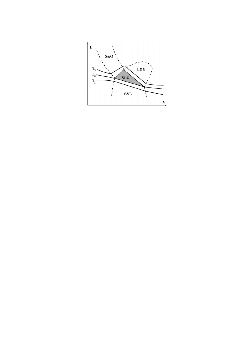
Fig. 8. This shows isotherms in the (º, ») plane near the triple point of a simple system. If one substituted pressure or
temperature for º or » as a coordinate then the full two-dimensional region would be compressed into a one-
dimensional region. In the triple point region the temperature is constant, which shows that isotherms need not be
one-dimensional curves.

two non-communicating pieces, and we have ruled out this pathology by fiat. However, another
possible pathology would be that an isotherm consists of several disconnected pieces, in which case
we could not pass from one side of an adiabat to another except by changing the temperature. Were
this to happen then the pictures in the textbooks would really be suspect, but fortunately, this
perversity does not occur, as we prove next.

There is one technical point that must first be noted. By concavity and differentiability of the

entropy, the range of the temperature function over

C is always an interval. There are no gaps. But

the range need not go from 0 to R — in principle. (Since we defined the state spaces of simple
systems to be open sets, the point 0 can never belong to the range.) Physical systems ideally always
cover the entire range (0,R), but there is no harm, and perhaps even a whiff of physical reality, in
supposing that the temperature range of the world is bounded. Recall that in axiom T5 we said that
the range must be the same for all systems and, indeed, for each choice of work coordinate within
a simple system. Thus, for an arbitrary simple system,

C, and »3o(C)

:"inf

+¹(X) : X3C,"inf+¹(º, ») : º3R such that (º, »)3C, ,

¹ :"sup+¹(

X) : X3

C,"sup+¹(º, ») : º3R such that (º, »)3C, .

Theorem 5.5 (Isotherms cut adiabats). Suppose XOXOX and X and X have equal temperatures,

(X)"¹(X)"¹.

(1)

If ¹(¹(¹ then there is a point X

X with ¹(X

)"¹. In other words: ¹he

isotherm through X cuts every adiabat between X and X.

(2)

If ¹"¹ , then either there is an X

X with ¹(X

)"¹, or, for any ¹(¹ there exist

points X

, X and X with XOX & XOX and ¹(X)"¹(X)"¹(X)"¹.

E.H. Lieb, J. Yngvason / Physics Reports 310 (1999) 1—96

(3)

If ¹"¹, then either there is an X

X with ¹(X

)"¹, or, for any ¹'¹ there exist

points X

, X and X with XOX & XOX and ¹(X)"¹(X)"¹(X)"¹.

Proof. Step 1. First we show that for every ¹ with ¹(¹(¹ the sets X:"

+½:¹(½)'¹, and X:"+½: ¹(½)(¹, are open and connected. The openness follows from

the continuity of ¹. Suppose that

X and X are non-empty, open sets satisfying X"X6X. We

shall show that

X5X is not empty, thereby showing that X is connected.By axiom T5, the range

of ¹, restricted to points (º, »)3

C, with » fixed, is independent of », and hence o(X)"o(C),

where

o denotes the projection (º, ») | ». It follows that o(X)6o(X)"o(C) and, since o is an

open mapping and

o(C) is connected, we have that o(X)5o(X) is not empty. Now if

(º,»)3XLX and if (º,»)3XLX, then, by the monotonicity of ¹(º,») in º for fixed », it

follows that the line joining (º,»)3X and (º,»)3X lies entirely in X"X6X. Since X and

X are open, X5X is not empty and X is connected. Similarly, X is connected.

Step 2. We show that if ¹(¹(¹ , then there exist points X, X, with X

and ¹(X)4¹4¹(X). We write the proof for X, the existence of X is shown in the same

way. In the case that »6

o(A6) the existence of X follows immediately from the monotonicity of

(º, ») in º for fixed ». If »6

, o(A6) we first remark that by axiom T5 and because ¹(¹

there exists X

OX with ¹(¹(X). Also, by monotonicity of ¹ in º there exists X with

OXOX and ¹(X)'¹. Hence X and X both belong to X, and XOXOX. Now X is

nonempty, open and connected, and

jA6 splits C!jA6 into disjoint, open sets. Hence X must cut

jA6, i.e., there exists an X3X5jA6.

Having established the existence of X and X we now appeal to continuity of ¹ and

connectedness of

jA6 (axiom S4) to conclude that there is an X3jA6 with ¹(X)"¹. This

completes the proof of assertion (1).

Step 3. If ¹"¹ and »6

o(A6), then the existence of X3jA6 with ¹(X)"¹ follows from

monotonicity of ¹ in º. Let us now assume that all points on

jA6 have temperatures strictly less

than ¹ . By axiom A5 and by continuity and monotonicity of ¹ in º, there is for every ¹(¹

an X

OX with ¹(X)"¹. For the same reasons there is an X with XOXOX and

)"¹. By the argument of step 2 there is thus an X3jA6 with ¹(X)"¹. Thus assertion

(2) is established. The case ¹"¹ (assertion (3)) is treated analogously.

䊏

5.3. Thermal equilibrium and uniqueness of entropy

In Section 2 we have encountered two general uniqueness theorems for entropy. The first,

Theorem 2.4, relies only on axioms A1—A6, and CH for the double scaled copies of

C, and states

that an entropy function on

C is uniquely determined, up to an affine transformation of scale, by

the relation

O on the double scaled copies. In the second, Theorem 2.10, it is further assumed that

the range of the entropy is connected which, in particular, is the case if the convex combination
axiom A7 holds. Under this condition the relation

O on C;C determines the entropy. Both these

uniqueness results are of a very general nature and rely only on the structure introduced in
Section 2. The properties of entropy and temperature that we have now established on the basis of
axioms A1—A7, S1—S3 and T1—T5, allow us to supplement these results now with a uniqueness
theorem of a different kind.

E.H. Lieb, J. Yngvason / Physics Reports 310 (1999) 1—96

Theorem 5.6 (Adiabats and isotherms in

C determine the entropy). ¸et O and OH be two relations on

the multiple scaled copies of a simple system

C satisfying axioms A1—A7, S1—S3 and ¹1—¹5. ¸et 2

and 2

denote the corresponding relations of thermal equilibrium between states in

C. If O and

OH coincide on C and the same holds for the relations 2

and 2

, then

O and OH coincide

everywhere. In other words: ¹he adiabats in

C together with the isotherms determine the relation O on

all multiple scaled copies of

C and hence the entropy is uniquely determined up to an affine

transformation of scale.

Proof. Let S and S

H be (concave and continuously differentiable) entropies characterizing respec-

tively the relations

O and OH. (The existence follows from axioms A1—A7, S1—S3, and T1—T4, as

shown in the previous sections.) For points X,½3

C we have S(X)"S(½) if and only if X

& ½

which holds if and only if S

H(X)"SH(½), because O and OH coincide on C by assumption. Hence

S and S

H have the same level sets, namely the adiabats of the simple system. Thus, we can write

H(X)"f (S(X))

for some strictly monotone function, f, defined on the range of S — which is some interval ILR. We
claim that f is differentiable on I and therefore

jSH

jº

(X)"f

(S(X))

jº

(X) .

(5.11)

To prove the differentiability note that

jS/jº is never zero (since S is strictly monotonic in º by

Planck’s principle, Theorem 3.4). This implies that for each fixed » in

o(C) the function º | S(º, »)

has a continuous inverse K(S,»). (This, in turn, implies that I is open.) Thus, if X"(º, ») and
S(º, »)"

p and if p,p,2 is any sequence of numbers converging to p, the sequence of numbers

ºH

:"K(

pH,») converges to º. Hence

H(ºH,»)!SH(º,»)

ºH!º

f (

pH)!f(p)

pH!p

S(ºH,»)!S(ºH,»)

ºH!º

from which we deduce the differentiability of f and the formula (5.11).

Now consider the function

G(X)"

jSH

jº

which is continuous because S and S

H are continuously differentiable and (jS/jº)O0. By

Eq. (5.11), with g"f

G(X)"g(S(X)) ,

and we now wish to prove that g:IPR is a constant function (call it a). This will prove our theorem
because it implies that

H(º, »)"aS(º, »)#B(») .

This, in turn, implies that B(») is constant on adiabats. However, the projection of an adiabat,

jA6,

on R

L is an open set (because the pressure, which defines the tangent planes, is finite everywhere).

E.H. Lieb, J. Yngvason / Physics Reports 310 (1999) 1—96

Thus, the projection

o(C) is covered by open sets on each of which B(») is constant. But o(C) is

connected (indeed, it is convex) and therefore B(») is constant on all of

o(C).

To show that g is constant, it suffices to show this locally. We know that X

| G(X)"g(S(X)) is

constant on adiabats, and it is also constant on isotherms because the level sets of

jS/jº and

jSH/jº both coincide with the isotherms. We now invoke the transversality property and Theorem
5.5. Let

pL be any fixed point in the range I of S, i.e., pL"S(XK) for some XK3C. By the transversality

property there are points X,X such that

p"S(X)(pL(S(X)"p

and X 2

X. Now let p"S(X) be any other point in the open interval (p, p). By Theorem 5.5

there are points X

K and X

X such that X

K and X both lie on the same isotherm (namely

the isotherm through X and X). But this means that g(p)"G(S(X))"G(S(XK))"g(pL), so g is

constant.

䊏

Remark. The transversality property is essential for this uniqueness theorem. As a counter-
example, suppose that every isotherm is an adiabat. Then any concave S that has the adiabats as its
level sets would be an acceptable entropy.

6. Mixing and chemical reactions

6.1. The difficulty of fixing entropy constants

We have seen in Sections 2 and 4 that the entropies of all simple systems can be calibrated once

and for all so that the entropy of any compound system made up of any combination of the basic
simple systems is exactly the sum of the individual entropies. This global entropy works (i.e., it
satisfies the entropy principle of Section 2.2 and tells us exactly which processes can occur) in those
cases in which the ‘masses’ of the individual systems are conserved. That is, splitting and
recombination of simple systems is allowed, but not mixing of different systems or (chemical or
nuclear) reactions.

Nature does allow us to mix the contents of different simple systems, however, (which is not to be

confused with the formation of a compound system). Thus, we can mix one mole of water and one
mole of alcohol to form two moles of whiskey. The entropy of the mixture is certainly not the sum
of the individual entropies, as would be the case if we were forming a compound system.
Nevertheless, our previous analysis, namely Theorem 2.5, does tell us the entropy of the mixture
— up to an additive constant! ¹he multiplicative constant can be, and will be henceforth, fixed by the
entropy function of one standard system, e.g., one mole of mercury. The reason that the multiplica-
tive constant is fixed for the mixture is, as we have stressed, the notion of thermal equilibrium.
Another way to say this is that once the unit of energy (say Joules) and of temperature (say Kelvin)
have been fixed, then the entropy of every system, simple and compound, is fixed up to an additive
constant. Our assumptions A1—A7, S1—S3 and T1—T5 guarantee this.

A similar discussion applies to chemical reaction products. After all, the solution of alcohol in

water can be considered a chemical reaction if one wishes. It requires a certain amount of chemical

E.H. Lieb, J. Yngvason / Physics Reports 310 (1999) 1—96

sophistication, which was not available before the enlightenment, to distinguish a mixture from
a chemical compound.

The question addressed in this section is this: to what extent can the additive constants (denoted

by the letter B, in conformity with Theorems 2.3 and 2.5) be determined so that whenever a mixture
or reaction occurs adiabatically we can say that the entropy has not decreased? To what extent is
this determination unique?

One thing that conceivably might have to be discarded, partially at least, is the idea that

comparability is an equivalence relation. As stated in Section 1, to have an equivalence relation
would require that whenever X

OZ and ½OZ then XO½ or ½OX (and similarly for ZOX and

O½). If one were to resort to the standard devices of semi-permeable membranes and van’t Hoff

boxes, as in the usual textbooks, then it would be possible to maintain this hypothesis, even for
mixing and chemical reactions. In that case, one would be able to prove that the additive entropy
constants are uniquely determined for all matter, once they have been chosen for the 92 chemical
elements.

Alas, van’t Hoff boxes do not exist in nature, except in imperfect form. For example, Fermi,

(1956, p. 101), in a discussion of the van’t Hoff box, writes that “The equilibria of gaseous reactions
can be treated thermodynamically by assuming the existence of ideal semi-permeable membranes”,
but then goes on to state that “We should notice, finally, that in reality no ideal semi-permeable
membranes exist. The best approximation of such a membrane is a hot palladium foil, which
behaves like a semi-permeable membrane for hydrogen”. Nevertheless, the rest of Fermi’s dis-
cussion is based on the existence of such membranes!

We are not saying that the comparison hypothesis must be discarded for chemical reactions and

mixtures; we are only raising the logical possibility. As a result, we shall try to organize our
discussion without using this hypothesis.

Therefore, we shall have to allow the possibility that if a certain kind of process is theoretically

possible then entropy increase alone does not determine whether it will actually occur; in particular
cases it might conceivably be necessary to have a certain minimum amount of entropy increase
before a reaction can take place. Moreover, the entropy principle of Section 2.2 conceivably
might not hold in full generality in the sense that there could be irreversible processes for which
entropy does not strictly increase. What we do show in this section is that it is possible,
nevertheless, to fix the entropy constants of all substances in such a way, that the entropy never
decreases in an adiabatic process. This weak form of the entropy principle is stated in Theorem 6.2.
However, it is only because of a technicality concerned with uncountably many dimensions that we
cannot prove the entropy principle in the strong form and there is no doubt that the ‘good case’
mentioned at the end of this section actually holds in the real world. For all practical purposes
we do have the strong form because the construction of the constants is done inductively in such
a way that at each stage it is not necessary to revise the constants previously obtained; this means
that in the finite world in which we live we are actually dealing, at any given moment, with the
countable case.

A significant point to notice about the additive constants, B, is that they must scale correctly

when the system scales; a somewhat subtler point is that they must also obey the additivity law
under composition of two or more systems,

C;C, in order that Eq. (2.4) holds. As we shall see in

Section 6.2, this latter requirement will not be met automatically and it will take a bit of effort to
achieve it.

E.H. Lieb, J. Yngvason / Physics Reports 310 (1999) 1—96

As a final introductory remark let us mention a computational device that is often used, and

which seems to eliminate the need for any special discussion about mixing, reactions or other
variations in the amount of matter. This device is simply to regard the amount of a substance (often
called the ‘particle number’ because of our statistical mechanical heritage) as just one more work
coordinate. The corresponding ‘pressure’ is called the chemical potential in this case. Why does this
not solve our problems? The answer, equally simply, is that the comparison hypothesis will not
hold within a state space since the extended state space will ‘foliate’ into sheets, in each of which the
particle number is fixed. Axiom S2 will fail to hold. If particle number is introduced as a work
coordinate then the price we will have to pay is that there will be no simple systems. Nothing will have
been gained. The question we address here is a true physical question and cannot be eliminated by
introducing a mathematical definition.

6.2. Determination of additive entropy constants

Let us consider a collection of systems (more precisely, state spaces), containing simple and/or

compound systems. Certain adiabatic state changes are possible, and we shall be mainly interested
in those that take us from one specified system to another, e.g., X

O½ with X3C and ½3C.

Although there are uncountably many systems (since, in our convention, changing the amount of
any component means changing the system), we shall always deal in the following with processes
involving only finitely many systems at one time. In our notation the process of making one mole of
water from hydrogen and oxygen is carried out by letting X be a state in the compound system
C consisting of one mole of H and one half mole of O and by taking ½ to be a state in the simple

system,

C, consisting of one mole of water.

Each system has a well defined entropy function, e.g., for

C there is S

, and we know from

Section 4 that these can be determined in such a way that the sum of the entropies increases in any
adiabatic process in any compound space

C;C;2 . Thus, if XG3CG and ½G3CG then

(X,X,2)O(½,½,2) if and only if S(X)#S(X)#24S(½)#S(½)#2 ,

(6.1)

where we have denoted S

by SG for short. The additive entropy constants do not matter here since

each function SG appears on both sides of this inequality.

Now we consider relations of the type

O½ with X3C, ½3C .

(6.2)

Our goal is to find constants B(

C), one for each state space C, in such a way that the entropy defined

S(X) :"S

(X)#B(

C) for X3C

(6.3)

satisfies

S(X)4S(½)

(6.4)

whenever Eq. (6.2) holds.

Additionally, we require that the newly defined entropy satisfies scaling and additivity under

composition. Since the initial entropies S

(X) already satisfy them, these requirements become

E.H. Lieb, J. Yngvason / Physics Reports 310 (1999) 1—96

conditions on the additive constants B(

C):

B(tC;tC)"tB(C)#tB(C)

(6.5)

for all state spaces

C, C under consideration and t,t'0.

As we shall see, the additivity requirement is not trivial to satisfy, the reason being that a given

substance, say hydrogen, can appear in many different compound systems with many different
ratios of the mole numbers of the constituents of the compound system.

The condition (6.4) means that

C)!B(C)4S

(½)!S

(X)

whenever X

O½. Let us denote by D(C, C) the minimal entropy difference for all adiabatic

processes that can take us from

C to C, i.e.,

C, C) :"inf+S

(½)!S

(X) : X

O½, .

(6.6)

It is to be noted that D(

C, C) can be positive or negative and D(C, C)OD(C, C) in general. Clearly

C, C)"0. Definition (6.6) makes sense only if there is at least one adiabatic process that goes

from

C to C, and it is convenient to define D(C, C)"#R if there is no such process. In terms of

the D(

C, C)’s condition (6.4) means precisely that

C, C)4B(C)!B(C)4D(C, C) .

(6.7)

Although D(

C, C) has no particular sign, we can assert the crucial fact that

C, C)4D(C, C) .

(6.8)

This is trivially true if D(

C, C)"#R or D(C, C)"#R. If both are (R the reason (6.8) is

true is simply (6.1): By the definition (6.6), there is a pair of states X3

C and ½3C such that XO½

and S

(½)!S

(X)"D(

C, C) (or at least as closely as we please). Likewise, we can find ¼3C and

C, such that ZO¼ and S

(¼)!S

(Z)"D(

C, C). Then, in the compound system C;C we

have that (X,Z)

O(¼,½), and this, by Eq. (6.1), implies Eq. (6.8). Thus D(C, C)'!R if there is at

least one adiabatic process from

C to C.

Some reflection shows us that consistency in the definition of the entropy constants B(

C) requires

us to consider all possible chains of adiabatic processes leading from one space to another via
intermediate steps. Moreover, the additivity requirement leads us to allow the use of a ‘catalyst’ in
these processes, i.e., an auxiliary system, that is recovered at the end, although a state change within
this system might take place.

For this reason we now define new quantities, E(

C, C) and F(C, C), in the following way. First,

for any given

C and C we consider all finite chains of state spaces, C"C,C,2,C,"C such that

CG,CG>)(R for all i, and we define

C, C) :"inf+D(C,C)#2#D(C,\,C,), ,

(6.9)

where the infimum is taken over all such chains linking

C with C. Note that E(C, C)4D(C, C)

and E(

C, C) could be (R even if there is no direct adiabatic process linking C and C, i.e.,

E.H. Lieb, J. Yngvason / Physics Reports 310 (1999) 1—96

C, C)"R. We then define

C, C) :"inf+E(C;C,C;C), ,

(6.10)

where the infimum is taken over all state spaces

C. (These are the ‘catalysts’.)

The following properties of F(

C, C) are easily verified:

C ,C)"0 ,

(6.11)

F(t

C, tC)"tF(C, C) for t'0 ,

(6.12)

C;C,C;C)4F(C,C)#F(C,C) ,

(6.13)

C;C,C;C)"F(C,C) for all C .

(6.14)

In fact, Eqs. (6.11) and (6.12) are also shared by the D’s and the E’s. The ‘subadditivity’ (6.13) holds
also for the E’s, but the ‘translational invariance’ (6.14) might only hold for the F’s.

From (6.13) and (6.14) it follows that the F’s satisfy the ‘triangle inequality’

C, C)4F(C, C)#F(C, C)

(6.15)

(put

C"C, C"C, C"C"C.) This inequality also holds for the E’s as is obvious from the

definition (6.9). A special case (using Eq. (6.11)) is the analogue of Eq. (6.8):

C, C)4F(C, C) .

(6.16)

(This is trivial if F(

C, C) or F(C, C) is infinite, otherwise use (6.15) with C"C.)

Obviously, the following inequalities hold:

C, C)4!E(C, C)4!F(C, C)4F(C, C)4E(C, C)4D(C, C) .

The importance of the F’s for the determination of the additive constants is made clear in the

following theorem:

Theorem 6.1 (Constant entropy differences). If

C and C are two state spaces then for any two points

C and ½3C

O½ if and only if S

(X)#F(

C, C)4S

(½) .

(6.17)

Remarks. (1). Since F(

C, C)4D(C, C) the theorem is trivially true when F(C, C)"#R, in the

sense that there is then no adiabatic process from

C to C. The reason for the title ‘constant entropy

differences’ is that the minimum jump between the entropies S

(X) and S

(½) for X

O½ to be

possible is independent of X.

(2). There is an interesting corollary of Theorem 6.1. We know, from the definition (6.6), that

O½ only if S

(X)#D(

C, C)4S

(½). Since D(

C, C)4F(C, C), Theorem 6.1 tells us two things:

O½ if and only if S

(X)#F(

C, C)4S

(½) ,

(6.18)

(X)#D(

C, C)4S

(½)

if and only if

(X)#F(

C, C)4S

(½) .

(6.19)

We cannot conclude from this, however, that D(

C, C)"F(C, C).

E.H. Lieb, J. Yngvason / Physics Reports 310 (1999) 1—96

Proof. The ‘only if ’ part is obvious because F(

C, C)4D(C, C), and thus our goal is to prove the ‘if’

part. For clarity, we begin by assuming that the infima in Eqs. (6.6), (6.9) and (6.10) are minima, i.e.,
there are state spaces

C,C,C,2,C, and states XG3CG and ½G3CG, for i"0,2,N and states

I 3C and ½I3C such that

I , X)O½

XGO½G> for i"1,2,N!1
X,O(½I,½)

(6.20)

and F(

C, C) is given by

C, C)"D(C;C,C)#D(C,C)#2#D(C,,C;C)

(½

I )#

SH(½H)!S

I )!

SH(XH) .

(6.21)

In (6.21) we used the abbreviated notation SH for S

and we used the fact that S

From the assumed inequality S

(X)#F(

C, C)4S

(½) and (6.21) we conclude that

(X)#S

(½

I )#

SH(½H)4S

I )#S

(½)#

SH(XH) .

(6.22)

However, both sides of this inequality can be thought of as the entropy of a state in the compound
space

CK :"C;C;C;C;2;C,. The entropy principle (6.1) for CK then tell us that

(X,½

I ,½,2,½,)O(XI,½,X,2,X,) .

(6.23)

On the other hand, using Eq. (6.20) and the axiom of consistency, we have that

I , X,X,2,X,)O(½I,½,½,2,½,) .

(6.24)

the

consistency

axiom

again,

have

from

Eq. (6.24)

that

I ,½, X,2,X,)O

(½,½

I ,½,½,2,½,). From transitivity we then have

(X,½

I ,½,½,2,½,)O(½,½I,½,½,2,½,) ,

and the desired conclusion, X

O½, follows from the cancellation law.

If F(

C, C) is not a minimum, then, for every e'0, there is a chain of spaces C,C,C,2,C, and

corresponding states as in Eq. (6.20) such that Eq. (6.21) holds to within

e and Eq. (6.22) becomes

(for simplicity of notation we omit the explicit dependence of the states and N on

(X)#S

(½

I )#

SH(½H)4S

I )#S

(½)#

SH(XH)#e .

(6.25)

Now choose any auxiliary state space

CI, with entropy function SI, and two states Z,Z3CI with

ZOOZ. The space C itself could be used for this purpose, but for clarity we regard CI as distinct.

Define

d(e) :"[SI(Z)!SI(Z)]\e. Recalling that dSI(Z)"SI(dZ) by scaling, we see that Eq. (6.25)

implies the following analogue of Eq. (6.23):

(

dZ,X,½I,½,2,½,)O(dZ,XI,½,X,2,X,) .

(6.26)

E.H. Lieb, J. Yngvason / Physics Reports 310 (1999) 1—96

Proceeding as before, we conclude that

(

dZ,X,½I,½,½,2,½,)O(dZ,½,½I,½,½,2,½,) ,

and thus (X,

dZ)O(½,dZ) by the cancellation law. However, dP0 as eP0 and hence XO½ by

the stability axiom.

䊏

According to Theorem 6.1 the determination of the entropy constants B(

C) amounts to satisfying

the estimates

C, C)4B(C)!B(C)4F(C, C)

(6.27)

together with the linearity condition (6.5). It is clear that Eq. (6.27) can only be satisfied with finite
constants B(

C) and B(C), if F(C, C)'!R. While the assumptions made so far do not exclude

C, C)"!R as a possibility, it follows from Eq. (6.16) that this can only be the case if at

the same time F(

C, C)"#R, i.e., there is no chain of intermediate adiabatic processes in the sense

described above that allows a passage from

C back to C. For all we know this is not the situation

encountered in nature and we exclude it by an additional axiom. Let us write

COC and say that

C is connected to C if F(C, C)(R, i.e. if there is a finite chain of state spaces, C,C,C,2,C, and

states such that Eq. (6.20) holds with X

I 3C and ½I3C. Our new axiom is the following:

(M) Absence of sinks. If

C is connected to C then C is connected to C, i.e., COCNCOC.

The introduction of this axiom may seem a little special, even artificial, but it is not. For one

thing, it is not used in Theorem 6.1 which, like the entropy principle itself, states the condition
under which adiabatic process from X to ½ is possible. Axiom M is only needed for setting the
additive entropy constants so that Eq. (6.17) can be converted into a statement involving S(X) and
S(½) alone, as in Theorem 6.2. Second, axiom M should not be misread as saying that if we can
make water from hydrogen and oxygen then we can make hydrogen and oxygen directly from
water (which requires hydrolysis). What it does require is that water can eventually be converted
into its chemical elements, but not necessarily in one step and not necessarily reversibly. The
intervention of irreversible processes involving other substances is allowed. Were axiom M to fail in
this case then all the oxygen in the universe would eventually turn up in water and we should have
to rely on supernovae to replenish the supply from time to time.

By axiom M (and the obvious transitivity of the relation

O for state spaces), connectedness

defines an equivalence relation between state spaces, and instead of

COC we can write

C&C

(6.28)

to indicate that the

O relation among state spaces goes both ways. As already noted, C&C is

equivalent to !R(F(

C, C)(R and !R(F(C, C)(R.

Without further assumptions (note, in particular, that no assumptions about ‘semi-permeable

membranes’ have been made) we can now derive the entropy principle in the following weak
version:

Theorem 6.2 (Weak form of the entropy principle). Assume axiom M in addition to A1—A7, S1—S3,
T1—T5. ¹hen the entropy constants B(

C) can be chosen in such a way that the entropy S, defined on all

E.H. Lieb, J. Yngvason / Physics Reports 310 (1999) 1—96

states of all systems by (6.3), satisfies additivity and extensivity (2.4), (2.5), and moreover

O½ implies S(X)4S(½) .

(6.29)

Proof. The proof is a simple application of the Hahn—Banach theorem (see, e.g., the appendix to
Giles (1964) and Reed and Simon (1972)). Consider the set S of all pairs of state spaces (

C, C). On

S we define an equivalence relation by declaring (

C, C) to be equivalent to (C;C,C;C) for all

C. Denote by [C,C] the equivalence class of (C,C) and let L be the set of all these equivalence

classes.

On L we define multiplication by scalars and addition in the following way:

C, C]:"[tC, tC] for t'0 ,

C, C]:"[!tC,!tC] for t(0 ,

C, C]:"[C, C]"[C, C] ,

[

C,C]#[C,C]:"[C;C,C;C] .

With these operations L becomes a vector space, which is infinite dimensional in general. The zero
element is the class [

C, C] for any C, because by our definition of the equivalence relation (C, C) is

equivalent to (

C;C, C;C), which in turn is equivalent to (C, C). Note that for the same reason

[

C, C] is the negative of [C, C].

Next, we define a function H on L by

H([

C, C]) :"F(C, C) .

Because of Eq. (6.14), this function is well defined and it takes values in (!R,R]. Moreover, it
follows from Eqs. (6.12) and (6.13) that H is homogeneous, i.e., H(t[

C, C])"tH([C, C]), and

subadditive, i.e., H([

C,C]#[C,C])4H([C,C])#H([C,C]). Likewise,

G([

C, C]) :"!F(C, C)

is homogeneous and superadditive, i.e., G([

C,C]#[C,C])5G([C,C])#G([C,C]). By

Eq. (6.16) we have G4F so, by the Hahn—Banach theorem, there exists a real-valued linear
function ¸ on L lying between G and H; i.e.,

C, C)4¸([C, C])4F(C, C) .

(6.30)

Pick any fixed

C and define

C) :"¸([C;C,C]) .

By linearity, ¸ satisfies ¸([

C, C])"!¸(![C, C])"!¸([C, C]). We then have

C)!B(C)"¸([C;C,C])#¸([C,C;C])"¸([C,C])

and hence Eq. (6.27) is satisfied.

䊏

From the proof of Theorem 6.2 it is clear that the indeterminacy of the additive constants B(

can be traced back to the non uniqueness of the linear function ¸([

C, C]) lying between

E.H. Lieb, J. Yngvason / Physics Reports 310 (1999) 1—96

G([

C, C])"!F(C, C) and H([C, C])"F(C, C). This non uniqueness has two possible sources:

One is that some pairs of state spaces

C and C may not be connected, i.e., F(C, C) may be infinite

(in which case F(

C, C) is also infinite by axiom M). The other possibility is that there is a finite, but

positive ‘gap’ between G and H, i.e.,

C, C)(F(C, C)

(6.31)

might hold for some state spaces, even if both sides are finite.

In nature only states containing the same amount of the chemical elements can be transformed

into each other. Hence F(

C, C)"#R for many pairs of state spaces, in particular, for those that

contain different amounts of some chemical element. The constants B(

C) are therefore never

unique: For each equivalence class of state spaces (with respect to &) one can define a constant
that is arbitrary except for the proviso that the constants should be additive and extensive under
composition and scaling of systems. In our world, where there are 92 chemical elements (or, strictly
speaking, a somewhat larger number, N, since one should count different isotopes as different
elements), and this leaves us with at least 92 free constants that specify the entropy of one mole of
each of the chemical elements in some specific state.

The other possible source of non uniqueness, a non-zero gap (6.31) is, as far as we know, not

realized in nature, although it is a logical possibility. The true situation seems rather to be the
following: The equivalence class [

C] (with respect to &) of every state space C contains a distin-

guished state space

K([C])"jC;2;j,C, ,

where the

CG are the state spaces of one mole of each of the chemical elements, and the numbers

(

j,2,j,) specify the amount of each chemical element in C. We have

K([tC])"tK([C]) ,

(6.32)

K([C;C])"K([C]);K([C]) .

(6.33)

Moreover (and this is the crucial ‘experimental fact’),

K([C]), C])"F(C, K([C]))

(6.34)

for all

C. Note that Eq. (6.34) is subject to experimental verification by measuring on the one hand

entropy differences for processes that synthesize chemical compounds from the elements (possibly
through many intermediate steps and with the aid of catalysts), and on the other hand for processes
where chemical compounds are decomposed into the elements.

It follows from Eqs. (6.15), (6.16) and (6.34) that

C, C)"F(C, K([C]))#F(K([C]), C) ,

(6.35)

C, C)"F(C, C)

(6.36)

for all

C&C. Moreover, an explicit formula for B(C) can be given in this good case:

C)"F(C, K([C]) .

(6.37)

E.H. Lieb, J. Yngvason / Physics Reports 310 (1999) 1—96

If F(

C, C)"R, then (6.27) holds trivially, while for C&C we have by Eqs. (6.35) and (6.36)

C)!B(C)"F(C, C)"!F(C, C) ,

(6.38)

i.e., the inequality (6.27) is saturated. It is also clear that in this case B(

C) is unique up to the choice

of arbitrary constants for the fixed systems

C,2,C,. The particular choice (6.37) corresponds to

putting B(

CG)"0 for the chemical elements i"1,2,N.

From Theorem 6.1 it follows that in the good case just described the comparison principle holds

in the sense that all states belonging to systems in the same equivalence class are comparable, and the
relation

O is exactly characterized by the entropy function, i.e., the full entropy principle holds.

If there is a genuine gap, Eq. (6.31), then for some pair of state spaces we might have only the

weak version of the entropy principle, Theorem 6.2. Moreover, it follows from Theorem 6.1 that in
this case there are no states X3

C and ½3C such that X

& ½

. Hence, in order for the full entropy

principle to hold as far as

C and C are concerned, it is only necessary to ensure that XOO½

implies S(X)(S(½), and this will be the case (again by Theorem 6.1) if and only if

C, C)(B(C)!B(C)(F(C, C) .

(6.39)

In other words, we would have the full entropy principle, gaps notwithstanding, if we could be sure

that whenever Eq. (6.31) holds then the inequalities in Eq. (6.30) are both strict inequalities.

We are not aware of a proof of the Hahn—Banach theorem that will allow us to conclude that

Eq. (6.30) is strict in all cases where Eq. (6.31) holds. If, however, the dimension of the linear space
L considered in the proof of Theorem 6.2 were finite then the Hahn—Banach theorem would allow
us to choose the B’s in this way. This is a consequence of the following lemma.

Lemma 6.1 (Strict Hahn–Banach). ¸et » be a finite dimensional, real vector space and p : »PR
subadditive, i.e., p(x#y)4p(x)#p(y) for all x, y3», and homogenous, i.e., p(

jx)"jp(x) for

all

j50, x3». ¹hen there is a linear functional ¸ on », such that !p(!x)4¸(x)4p(x) for all

x3». Moreover, for those x for which !p(!x)(p(x) holds we have the strict inequalities

p(!x)(¸(x)(p(x).

Proof. Note first that subadditivity implies that p(x)!p(!y)4p(x#y)4p(x)#p(y) for all
x, y3».

Define

»"+

x: !p(!x)"p(x)

,. If x3» and y3», then p(x)#p(y)"

p(x)!p(!y)4p(x#y)4p(x)#p(y) and hence p(x)#p(y)"p(x#y). (Note that x need not
belong to ».) If x3» and j50, then p(jx)"jp(x)"j(!p(!x))"!p(!jx), and if j(0 we

have, in the same way, p(

jx)"p((!j)(!x))"(!j)p(!x)"j(!p(!x))"jp(x). Thus » is

a linear space, and p is a linear functional on it. We define ¸(x)"p(x) for x3».

Let »

be an algebraic complement of », i.e., all x3» can be written as x"y#z with y3»,

z3»

and the decomposition is unique if xO0. On » the strict inequality !p(!x)(p(x) holds

for all xO0. If ¸ can be defined on »

such that !p(!x)(¸(x)(p(x) for all »UxO0 we

reach our goal by defining ¸(x#y)"¸(x)#¸(y) for x3»

, y3». Hence it suffices to consider

the case that »"+0,.

E.H. Lieb, J. Yngvason / Physics Reports 310 (1999) 1—96

Now suppose »L» is a linear space and ¸ has been extended from +0, to » such that our

requirements are fulfilled on », i.e., !p(!x)(¸(x)(p(x) for x3», xO0. Define, for x3»

N (x)" inf

WZ4

+p(x#y)!¸(y), .

By subadditivity it is clear that for all x

p(!x)4!p

N (!x)4pN(x)4p(x) .

Since » is finite dimensional (by assumption) and p continuous (by convexity) the infimum is, in
fact, a minimum for each x, i.e., p

N (x)"p(x#y)!¸(y) with some y3», depending on x.

Suppose » is not the whole of ». Pick x linearly independent of ». On the space spanned by

and x we define

(

jx#x)"(j/2)(pN(x)!pN(!x))#¸(x) .

if x3», j3R.

Then

jx#x)!¸(jx#x)"p(jx#x)!¸(x)!¸(jx)5pN(jx)!¸(jx)50

and equality holds in the last inequality if and only if p

N (jx)"!pN(!jx), i.e.,

jx#y)#p(!jx#y)"¸(y#y)4p(y#y) .

(6.40)

for some y, y

3» (depending on jx). On the other hand,

jx#y)#p(!jx#y)5p(y#y)

by subadditivity, so Eq. (6.40) implies

(y#y

)"p(y#y) .

(6.41)

By our assumption about » this hold only if y#y"0. But then

p(!

jx#y)"p(!jx!y)

and from Eqs. (6.40) and (6.41) we get !p(!

jx!y)"p(jx#y) and hence jx"!y3».

Since x , » this is only possible for j"0, in which case p(x)"¸(x) and hence (by our

assumption about »), x"0. Thus the statement ¸(x)"p(x) for some x lying in the span of

» and

x implies that x"0. In the same way one shows that ¸(x)"!p(!x) implies x"0.

Thus, we have succeeded in extending ¸ from » to the larger space span+»,x,. Proceeding by

induction we obtain ¸ satisfying our requirements on all ».

䊏

Since the proof of the above version of the Hahn—Banach theorem proceeds inductively over

subspaces of increasing dimension it generalizes in a straightforward way to spaces of countable
algebraic dimension. Moreover, in such spaces the condition (6.39) could be fulfilled at any
induction step without modifying the constants previously defined. Hence, even in cases where
Eq. (6.36) is violated, this hypothetical weakening of the full entropy principle could never be
detected in real experiments involving only finitely many systems.

E.H. Lieb, J. Yngvason / Physics Reports 310 (1999) 1—96

7. Summary and conclusions

In this final section we recall our notation for the convenience of the reader and collect all the

axioms introduced in Sections 2—4 and 6. We then review the logical structure of the paper and the
main conclusions.

Our axioms concern equilibrium states, denoted by X,½, etc., and the relation

O of adiabatic

accessibility between them. If X

O½ and ½OX we write X

& ½

, while X

OO½ means that XO½,

but not ½

OX. States belong to state spaces C, C,

2 of systems, that may be simple or compound.

The composition of two state spaces

C, C is the Cartesian product C;C (the order of the factors is

unimportant); the composition of X3

C and ½3C is denoted (X,½)3C;C. A state X3C may be

scaled by a real parameter t'0, leading to a state tX in a scaled state space

CR, sometimes written

C. For simple systems the states are parametrized by the energy coordinate º3R and the work

coordinates »3R

The axioms are grouped as follows:

7.1. General axioms

(A1) Reflexivity. X

(A2) Transitivity. X

O½ and ½OZ implies XOZ.

(A3) Consistency. X

OX and ½O½ implies (X,½)O(X,½).

(A4) Scaling invariance. If X

O½, then tXOt½ for all t'0.

(A5) Splitting and recombination. For 0(t(1, X

(tX, (1!t)X).

(A6) Stability. If (X,

eZ)O(½,eZ) holds for a sequence of e’s tending to zero and some states Z,

Z, then XO½.

(A7) Convex combination. Assume X and ½ are states in the same state space,

C, that has a convex

structure. If t3[0, 1] then (tX, (1!t)½)

OtX#(1!t)½.

7.2. Axioms for simple systems

Let

C, a convex subset of RL> for some n'0, be the state space of a simple system.

(S1)

Irreversibility. For each X3

C there is a point ½3C such that XOO½. (Note: This axiom is

implied by T4, and hence it is not really independent.)

(S2)

Lipschitz tangent planes. For each X3

C the forward sector A6"+½3C: XO½, has

a unique support plane at X (i.e., A6 has a tangent plane at X). The slope of the tangent plane

is assumed to be a locally ¸ipschitz continuous function of X.

(S3)

Connectedness of the boundary. The boundary

jA6 of a forward sector is connected.

7.3. Axioms for thermal equilibrium

(T1) Thermal contact. For any two simple systems with state spaces

C and C, there is another

simple system, the thermal join of

C and C, with state space

D"+(º,»,»): º"º#º with (º,»)3C,(º,»)3C, .

E.H. Lieb, J. Yngvason / Physics Reports 310 (1999) 1—96

Moreover,

C;CU((º,»), (º,»))O(º#º,»,»)3D .

(T2) Thermal splitting. For any point (º, »,»)3D there is at least one pair of states,

(º,»)3C, (º,»)3C, with º"º#º, such that

(º, »,»)

((º,»), (º,»)) .

In particular, if (º, ») is a state of a simple system

C and j3[0, 1] then

(º, (1!

j)», j»)

(((1!

j)º, (1!j)»), (jº, j»))3C\H;CH .

If (º, »,»)

((º,»),(º,»)) we write (º,») 2

(º,»).

(T3) Zeroth law. If X 2

& ½

and if ½ 2

Z then X 2

(T4) Transversality. If

C is the state space of a simple system and if X3C, then there exist states

X 2

X with XOOXOOX.

(T5) Universal temperature range. If

C and C are state spaces of simple systems then, for every

C and every » in the projection of C onto the space of its work coordinates, there is

a ½3

C with work coordinates » such that X 2& ½.

7.4. Axiom for mixtures and reactions

Two state spaces,

C and C are said to be connected, written COC, if there are state spaces

C,C,C,2,C, and states XG3CG and ½G3CG, for i"1,2,N and states XI3C and ½I3C such

that (X

I , X)O½, XGO½G> for i"1,2,N!1, and X,O(½I,½).

(M) Absence of sinks. If

C is connected to C then C is connected to C, i.e., COCNCOC.

The main goal of the paper is to derive the entropy principle (EP) from these properties of

here is a function, called entropy and denoted by S, on all states of all simple and compound

systems, such that

(a)

Monotonicity: If X

OO½, then S(X)(S(½), and if X

& ½

, then S(X)"S(½).

(b)

Additivity and extensivity: S((X, X

))"S(X)#S(X) and S(tX)"tS(X).

Differentiability of S as function of the energy and work coordinates of simple systems is also

proved and temperature is derived from entropy.

A central result on our road to the EP is a proof, from our axioms, of the comparison hypothesis

(CH) for simple and compound systems, which says that for any two states X,½ in the same state
space either X

O½ or ½OX holds. This is stated in Theorem 4.8. The existence of an entropy

function is discussed already in Section 2 on the basis of Axioms A1—A6 alone assuming in addition
CH. In the subsequent sections CH is derived from the other axioms. The main steps involved in
this derivation of CH are as follows.

The comparison hypothesis (which, once proved, is more appropriately called the comparison

principle) is first derived for simple systems in Theorem 3.7 in Section 3. This proof uses both the
special axioms S1—S3 of Section 3 and the general axioms A1—A7 introduced in Section 2. On the

E.H. Lieb, J. Yngvason / Physics Reports 310 (1999) 1—96

other hand, it should be stressed that Theorem 3.7 is independent of the discussion in Sections 2.4
and 2.5, where an entropy function is constructed, assuming the validity of CH.

The extension of CH to compound systems relies heavily on the axioms for thermal equilibrium

that are discussed in Section 4. The key point is that by forming the thermal join of two simple
systems we obtain a new simple system to which Theorem 3.7 can be applied. The extension of CH
from simple to compound systems is first carried out for products of scaled copies of the same
simple system (Theorem 4.4). Here the transversality axiom T4 plays an essential role by reducing
the consideration of states of the compound system that are not in thermal equilibrium to states in
the thermal join.

The proof of CH for products of different simple systems requires more effort. The main step here

is to prove the existence of ‘entropy calibrators’ (Theorem 4.7). This says that for each pair of simple
systems

C,C there exist four states, X,X3C, ½,½3C such that XOOX, ½OO½, but

(X,½)

(X, X). In establishing this property, we find it convenient to make use of the existence

of an entropy function for each of the spaces

C and C separately, which, as shown in Sections 2.4

and 2.5, follows from axioms A1—A6 and the already established property CH for products of
scaled copies of the same simple system.

Once CH has been established for arbitrary products of simple systems the entropy principle for

all adiabatic state changes, except for mixing of different substances and chemical reactions, follows
from the considerations of Sections 2.4 and 2.5. An explicit formula for S is given in Eq. (2.20): We
pick a reference system with two states ZOOZ, and for each system C a reference point X

C is

chosen in such a way that XR

and X

, X

). Then, for X3

S(X)"sup

+j: (X

jZ)O(X,jZ), .

(For

j(0, (X

jZ)O(X,jZ) means, per definition, that (X

jZ)O(X,!jZ), and for j"0

that X

OX.)

In Section 5 we prove that for a simple system the entropy function is a once continuously

differentiable function of the energy and the work coordinates. The convexity axiom A7, which
leads to concavity of the entropy, and the axiom S2 (Lipschitz tangent planes) are essential here.
We prove that the usual thermodynamic relations hold, in particular ¹"(

jS/jº)\ defines the

absolute temperature. Up to this point neither temperature nor hotness and coldness have actually
been used. In this section we also prove (in Theorem 5.6) that the entropy for every simple system is
uniquely determined, up to an affine change of scale, by the level sets of S and ¹, i.e., by the adiabats
and isotherms regarded only as sets, and without numerical values.

In the final Section 6 we discuss the problem of fixing the additive entropy constants when

processes that change the system by mixing and chemical reactions are taken into account. We
show that, even without making any assumptions about the existence of unrealistic semi-permeable
membranes, it is always possible to fix the constants in such a way that the entropy remains
additive, and never decreases under adiabatic processes. This is not quite the full entropy principle,
since there could still be states with X

OO½, but S(X)"S(½). This abnormal possibility, however,

is irrelevant in practice, and we give a necessary and sufficient condition for the situation to occur
that seems to be realized in nature: The entropy of every substance is uniquely determined once an
arbitrary entropy constant has been fixed for each of the chemical elements, and X

OO½ implies

that S(X)(S(½).

E.H. Lieb, J. Yngvason / Physics Reports 310 (1999) 1—96

After this summary of the logical structure of the paper we add some remarks on the relation of

our treatment of the second law and more conventional formulations, e.g., the classical statements
of Kelvin, Clausius and Carathe´odory paraphrased in Section 1.1. What immediately strikes the
eye is that these classical formulations are negative statements: They claim that certain processes
are not possible. Thus, the Clausius formulation essentially says that thermal contact leads to an
irreversible process. On the other hand, what the founding fathers seem to have taken for granted,
is that there also exist reversible processes. Thus the Clausius inequality,

dQ/¹40, which

ostensibly follows from his version of the second law and is the starting point for most textbook
discussions of entropy, does not by itself lead to an entropy function. What is needed in this
formulation is the existence of reversible processes, where equality holds (or at least processes that
approximate equality arbitrarily closely). One might even question the possibility of attaching
a precise meaning to ‘

dQ’ and ‘¹’ for irreversible processes. (See, however, Eq. (5.8) and the

discussion preceding it, where the symbols are given a precise meaning in a concrete situation.)

The basic question we set out to examine is this: Why can adiabatic processes within a system be

exactly characterized by the increase (more precisely, non-decrease) of an additive entropy func-
tion? In Section 2, where the comparison principle CH is assumed, an answer is already given: It is
because all reasonable notions of adiabatic accessibility should satisfy axioms A1—A6, and these
axioms, together with CH, are equivalent to the existence of an additive entropy function that
characterizes the relation. This is expressed in Theorem 2.2. If we now look at axioms A1—A6 and
the comparison principle we see that these are all positive statements about the relation

O: They all

say that certain elementary processes are possible (provided some other processes are possible), and
none of them says that some processes are impossible. In particular, the trivial case, when
everything is accessible form everything else, is not in conflict with A1—A6 and the comparison
principle: It corresponds to a constant entropy.

From this point of view the existence of an entropy function is an issue that can, to a large extent,

be discussed independently of the second law, as originally formulated by the founders (as given in
Section 1.1). ¹he existence of entropy has more to do with comparability of states and reversibility
than with irreversibility. In fact, one can conceive of mathematical examples of a relation

O that

is characterized by a function S and satisfies A1—A6 and CH, but S is constant in a whole
neighborhood of some points — and the Clausius inequality fails. Conversely, the example of the
‘world of thermometers’, discussed in Section 4.4 and Fig. 7 is relevant in this context. Here the
second law in the sense of Clausius holds, but the Clausius equality

dQ/¹"0 cannot be achieved

and there is no entropy that characterizes the relation for compound systems!

In our formulation the reversibility required for the definition of entropy is a consequence of the

comparison principle and the stability axiom A3. (The latter allows us to treat reversible processes
as limiting cases of irreversible processes, which are, strictly speaking the only processes realized in
nature.) This is seen most directly in Lemma 2.3, which characterizes the entropy of a state in terms
of adiabatic equivalence of this state with another state in a compound system. This lemma depends
crucially on CH (for the compound system) and A3.

So one may ask what, in our formulation, corresponds to the negative statements in the classical

versions of the second law. The answer is: It is axiom S1, which says that from every state of
a simple system one can start an irreversible adiabatic process. In combination with A1—A6 and the
convexity axiom A7, this is equivalent to Carathe´odory’s principle. Moreover, together with the
other simple system axioms, in particular the assumption about the pressure, S2, it leads to

E.H. Lieb, J. Yngvason / Physics Reports 310 (1999) 1—96

Planck’s principle, Theorem 3.4, which states the impossibility of extracting energy adiabatically
from a simple system at fixed work coordinates. Hence, the entropy not only exists, but also it is
nowhere locally constant. This additional property of entropy is a precise version of the classical
statements of the second law. By contrast, an entropy having level sets like the temperature in
Fig. 8 would allow the construction of a perpetual motion machine of the second kind.

It would be mistake, however, to underestimate the role played by the axioms other than S1.

They are all part of the structure of thermodynamics as presented here, and conspire to produce an
entropy function that separates precisely the possible from the impossible and has the convexity
and regularity properties required in the practical application of thermodynamics.

Acknowledgements

We are deeply indebted to Jan Philip Solovej for many useful discussions and important insights,

especially in regard to Sections 3 and 6. Our thanks also go to Fredrick Almgren for helping us
understand convex functions, to Roy Jackson, Pierluigi Contucci, Thor Bak and Bernhard
Baumgartner for critically reading our manuscript and to Martin Kruskal for emphasizing the
importance of Giles’ book to us. We thank Robin Giles for a thoughtful and detailed review with
many helpful comments. We thank John C. Wheeler for a clarifying correspondence about the
relationship between adiabatic processes, as usually understood, and our definition of adiabatic
accessibility. Some of the rough spots in our story were pointed out to us by various people during
various public lectures we gave, and that is also very much appreciated.

A significant part of this work was carried out at Nordita in Copenhagen and at the Erwin

Schro¨dinger Institute in Vienna; we are grateful for their hospitality and support.

Appendix A

A.1. ¸ist of symbols

A.1.1. Some standard mathematical symbols
a3A or A U a

means ‘the point a is an element of the set A’.

, A

means ‘the point a is not an element of the set A’.

ALB or BMA

means ‘the set A is in the set B’.

is the set of objects that are in the set A and in the set B.

is the set of objects that are either in the set A or in the set B or in both sets.

is the set consisting of pairs (a, b) with a3A and b3B.

+a : P,

means the set of objects a having property P.

a :"b or b": a

means ‘the quantity a is defined by b’.

PNQ

means ‘P implies Q’.

is n-dimensional Euclidean space whose points are
n-tuples(x,2, xL) of real numbers.

[s, t]

means the closed interval s4x4t.

means the boundary of a set A.

E.H. Lieb, J. Yngvason / Physics Reports 310 (1999) 1—96

A.1.2. Special symbols
X

O½

(‘X precedes ½’) means that the state ½ is
adiabatically accessible from the state X.

(Section 2.1.2)

O.½

(‘X does not precede ½’) means that ½ is not adiabatically
accessible from X.

(Section 2.1.2)

OO½

(‘X strictly precedes ½’) means that ½ is adiabatically
accessible from X, but X is not accessible from ½.

(Section 2.1.2)

& ½

(‘X is adiabatically equivalent to ½’) means that
X

O½ and ½OX.

(Section 2.1.2)

X 2

& ½

means that the states X and ½ are in thermal equilibrium.

(Section 4.1)

the ‘forward sector’ of a state X3

C, i.e., +½3C: XO½,.

(Section 2.6)

a copy of the state X, but scaled by a factor t.

(Section 2.1.1)

the state space consisting of scaled states tX, with X3

(Section 2.1.1)

tX#(1!t)½

a convex combination of states X and ½ in a
state space with a convex structure.

(Section 2.6)

R(X,X)

the ‘strip’

+X3C : XOXOX, between the adiabats

through X and X3C, XOX.

(Section 2.4)

the projection of

jA6 onto the space of work coordinates,

for X in the state space of a simple system

CLRL>,

i.e.,

o6"+»3RL:(º,»)3jA6 for some º3R,.

(Section 3.3)

the projection onto the space of work coordinates of a
simple system

i.e., if X"(º, »)3

C, then o(X)"».

(Section 4.1)

A.2. Index of technical terms

Additivity of entropy . . . . . . . . . . . . . . . . . . . . . . . . . . . . . . . . . . . . . . . . . . . . . . . . . . . . . . . . . . . . . . .

(Section 2.2)

Adiabat . . . . . . . . . . . . . . . . . . . . . . . . . . . . . . . . . . . . . . . . . . . . . . . . . . . . . . . . . . . . . . . . . . . . . . . . . . . . .

(Section 3.2)

Adiabatic accessibility . . . . . . . . . . . . . . . . . . . . . . . . . . . . . . . . . . . . . . . . . . . . . . . . . . . . . . . . . . . . . .

(Section 2.1.2)

Adiabatic equivalence . . . . . . . . . . . . . . . . . . . . . . . . . . . . . . . . . . . . . . . . . . . . . . . . . . . . . . . . . . . . . .

(Section 2.1.2)

Adiabatic process . . . . . . . . . . . . . . . . . . . . . . . . . . . . . . . . . . . . . . . . . . . . . . . . . . . . . . . . . . . . . . . . . . .

(Section 2.1.1)

Boundary of a forward sector . . . . . . . . . . . . . . . . . . . . . . . . . . . . . . . . . . . . . . . . . . . . . . . . . . . . .

(Section 3.2)

Canonical entropy . . . . . . . . . . . . . . . . . . . . . . . . . . . . . . . . . . . . . . . . . . . . . . . . . . . . . . . . . . . . . . . . . .

(Section 2.4)

Cancellation law . . . . . . . . . . . . . . . . . . . . . . . . . . . . . . . . . . . . . . . . . . . . . . . . . . . . . . . . . . . . . . . . . . . .

(Section 2.3)

Carathe´odory+s principle . . . . . . . . . . . . . . . . . . . . . . . . . . . . . . . . . . . . . . . . . . . . . . . . . . . . . . . . . .

(Section 2.7)

Carnot efficiency . . . . . . . . . . . . . . . . . . . . . . . . . . . . . . . . . . . . . . . . . . . . . . . . . . . . . . . . . . . . . . . . . . . .

(Section 5.1)

Comparable states . . . . . . . . . . . . . . . . . . . . . . . . . . . . . . . . . . . . . . . . . . . . . . . . . . . . . . . . . . . . . . . . . .

(Section 2.1.2)

Comparison hypothesis (CH) . . . . . . . . . . . . . . . . . . . . . . . . . . . . . . . . . . . . . . . . . . . . . . . . . . . . . .

(Section 2.3)

Composition of systems . . . . . . . . . . . . . . . . . . . . . . . . . . . . . . . . . . . . . . . . . . . . . . . . . . . . . . . . . . . .

(Section 2.1.1)

Consistent entropies . . . . . . . . . . . . . . . . . . . . . . . . . . . . . . . . . . . . . . . . . . . . . . . . . . . . . . . . . . . . . . . .

(Section 2.5)

Convex state space . . . . . . . . . . . . . . . . . . . . . . . . . . . . . . . . . . . . . . . . . . . . . . . . . . . . . . . . . . . . . . . . .

(Section 2.6)

Degenerate simple system ("thermometer) . . . . . . . . . . . . . . . . . . . . . . . . . . . . . . . . . . . . . .

(Section 3.1)

Entropy . . . . . . . . . . . . . . . . . . . . . . . . . . . . . . . . . . . . . . . . . . . . . . . . . . . . . . . . . . . . . . . . . . . . . . . . . . . . .

(Section 2.2)

Entropy calibrator . . . . . . . . . . . . . . . . . . . . . . . . . . . . . . . . . . . . . . . . . . . . . . . . . . . . . . . . . . . . . . . . .

(Section 4.1)

E.H. Lieb, J. Yngvason / Physics Reports 310 (1999) 1—96

Entropy constants . . . . . . . . . . . . . . . . . . . . . . . . . . . . . . . . . . . . . . . . . . . . . . . . . . . . . . . . . . . . . . . . . .

(Section 2.5)

Entropy function on a state space . . . . . . . . . . . . . . . . . . . . . . . . . . . . . . . . . . . . . . . . . . . . . . . .

(Section 2.4)

Entropy principle (EP) . . . . . . . . . . . . . . . . . . . . . . . . . . . . . . . . . . . . . . . . . . . . . . . . . . . . . . . . . . . . .

(Section 2.2)

Extensivity of entropy . . . . . . . . . . . . . . . . . . . . . . . . . . . . . . . . . . . . . . . . . . . . . . . . . . . . . . . . . . . . . .

(Section 2.2)

First law of thermodynamics . . . . . . . . . . . . . . . . . . . . . . . . . . . . . . . . . . . . . . . . . . . . . . . . . . . . . .

(Section 3.1)

Forward sector . . . . . . . . . . . . . . . . . . . . . . . . . . . . . . . . . . . . . . . . . . . . . . . . . . . . . . . . . . . . . . . . . . . . .

(Section 2.6)

Generalized ordering . . . . . . . . . . . . . . . . . . . . . . . . . . . . . . . . . . . . . . . . . . . . . . . . . . . . . . . . . . . . . . .

(Section 2.4)

Internal energy . . . . . . . . . . . . . . . . . . . . . . . . . . . . . . . . . . . . . . . . . . . . . . . . . . . . . . . . . . . . . . . . . . . . .

(Section 3.1)

Irreversible process . . . . . . . . . . . . . . . . . . . . . . . . . . . . . . . . . . . . . . . . . . . . . . . . . . . . . . . . . . . . . . . . .

(Section 2.7)

Isotherm . . . . . . . . . . . . . . . . . . . . . . . . . . . . . . . . . . . . . . . . . . . . . . . . . . . . . . . . . . . . . . . . . . . . . . . . . . . .

(Section 4.1)

Lipschitz continuity . . . . . . . . . . . . . . . . . . . . . . . . . . . . . . . . . . . . . . . . . . . . . . . . . . . . . . . . . . . . . . . .

(Section 3.2)

Lower temperature . . . . . . . . . . . . . . . . . . . . . . . . . . . . . . . . . . . . . . . . . . . . . . . . . . . . . . . . . . . . . . . . .

(Section 5.1)

Multiple scaled copy . . . . . . . . . . . . . . . . . . . . . . . . . . . . . . . . . . . . . . . . . . . . . . . . . . . . . . . . . . . . . . .

(Section 2.1.1)

Planck+s principle . . . . . . . . . . . . . . . . . . . . . . . . . . . . . . . . . . . . . . . . . . . . . . . . . . . . . . . . . . . . . . . . . .

(Section 3.3)

Pressure . . . . . . . . . . . . . . . . . . . . . . . . . . . . . . . . . . . . . . . . . . . . . . . . . . . . . . . . . . . . . . . . . . . . . . . . . . . . .

(Section 3.2)

Reference points for entropy . . . . . . . . . . . . . . . . . . . . . . . . . . . . . . . . . . . . . . . . . . . . . . . . . . . . . . .

(Section 2.4)

Second law of thermodynamics . . . . . . . . . . . . . . . . . . . . . . . . . . . . . . . . . . . . . . . . . . . . . . . . . . .

(Section 2.2)

Scaled copy . . . . . . . . . . . . . . . . . . . . . . . . . . . . . . . . . . . . . . . . . . . . . . . . . . . . . . . . . . . . . . . . . . . . . . . . .

(Section 2.1.1)

Scaled product . . . . . . . . . . . . . . . . . . . . . . . . . . . . . . . . . . . . . . . . . . . . . . . . . . . . . . . . . . . . . . . . . . . . . .

(Section 2.1.1)

Simple system . . . . . . . . . . . . . . . . . . . . . . . . . . . . . . . . . . . . . . . . . . . . . . . . . . . . . . . . . . . . . . . . . . . . . . .

(Section 3)

Stability . . . . . . . . . . . . . . . . . . . . . . . . . . . . . . . . . . . . . . . . . . . . . . . . . . . . . . . . . . . . . . . . . . . . . . . . . . . . .

(Section 2.3)

State . . . . . . . . . . . . . . . . . . . . . . . . . . . . . . . . . . . . . . . . . . . . . . . . . . . . . . . . . . . . . . . . . . . . . . . . . . . . . . . . .

(Section 2.1.1)

State space . . . . . . . . . . . . . . . . . . . . . . . . . . . . . . . . . . . . . . . . . . . . . . . . . . . . . . . . . . . . . . . . . . . . . . . . . .

(Section 2.1.1)

Subsystem . . . . . . . . . . . . . . . . . . . . . . . . . . . . . . . . . . . . . . . . . . . . . . . . . . . . . . . . . . . . . . . . . . . . . . . . . . .

(Section 2.1.1)

System . . . . . . . . . . . . . . . . . . . . . . . . . . . . . . . . . . . . . . . . . . . . . . . . . . . . . . . . . . . . . . . . . . . . . . . . . . . . . . .

(Section 2.1.1)

Temperature . . . . . . . . . . . . . . . . . . . . . . . . . . . . . . . . . . . . . . . . . . . . . . . . . . . . . . . . . . . . . . . . . . . . . . . .

(Section 5.1)

Thermal contact . . . . . . . . . . . . . . . . . . . . . . . . . . . . . . . . . . . . . . . . . . . . . . . . . . . . . . . . . . . . . . . . . . . .

(Section 4.1)

Thermal equilibration . . . . . . . . . . . . . . . . . . . . . . . . . . . . . . . . . . . . . . . . . . . . . . . . . . . . . . . . . . . . . .

(Section 4.1)

Thermal equilibrium . . . . . . . . . . . . . . . . . . . . . . . . . . . . . . . . . . . . . . . . . . . . . . . . . . . . . . . . . . . . . . .

(Section 4.1)

Thermal join . . . . . . . . . . . . . . . . . . . . . . . . . . . . . . . . . . . . . . . . . . . . . . . . . . . . . . . . . . . . . . . . . . . . . . . .

(Section 4.1)

Thermal reservoir . . . . . . . . . . . . . . . . . . . . . . . . . . . . . . . . . . . . . . . . . . . . . . . . . . . . . . . . . . . . . . . . . .

(Section 5.1)

Thermal splitting . . . . . . . . . . . . . . . . . . . . . . . . . . . . . . . . . . . . . . . . . . . . . . . . . . . . . . . . . . . . . . . . . . .

(Section 3.3)

Thermometer ("degenerate simple system) . . . . . . . . . . . . . . . . . . . . . . . . . . . . . . . . . . . . .

(Section 3.1)

Transversality . . . . . . . . . . . . . . . . . . . . . . . . . . . . . . . . . . . . . . . . . . . . . . . . . . . . . . . . . . . . . . . . . . . . . . .

(Section 4.1)

Upper temperature . . . . . . . . . . . . . . . . . . . . . . . . . . . . . . . . . . . . . . . . . . . . . . . . . . . . . . . . . . . . . . . . .

(Section 5.1)

Work coordinate . . . . . . . . . . . . . . . . . . . . . . . . . . . . . . . . . . . . . . . . . . . . . . . . . . . . . . . . . . . . . . . . . . .

(Section 3.1)

Zeroth law of thermodynamics . . . . . . . . . . . . . . . . . . . . . . . . . . . . . . . . . . . . . . . . . . . . . . . . . . . .

(Section 4.1)

References

Arens, R., 1963. An axiomatic basis for classical thermodynamics. J. Math. Anal. and Appl. 6, 207—229.
Bazarow, I.P., 1964. Thermodynamics. Pergamon Press, Oxford.
Bernstein, B., 1960. Proof of Carathe´odory’s local theorem and its global application to thermodynamics. J. Math. Phys.

1, 222—264.

E.H. Lieb, J. Yngvason / Physics Reports 310 (1999) 1—96

Borchers, H.J., 1981. Some remarks on the second law of thermodynamics. Rep. Math. Phys. 22, 29—48.
Born, M., 1964. Natural Philosophy of Cause and Chance. Dover, New York.
Born M., 1921. Kritische Bemerkungen zur traditionellen Darstellung der Thermodynamik. Phys. Zeits. 22, 218—224,

249—254, 282—286.

Boyling, J.B., 1968. Carathe´odory’s principle and the existence of global integrating factors. Commun. Math. Phys. 10,

52—68.

Boyling, J.B., 1972. An axiomatic approach to classical thermodynamics. Proc. Roy. Soc. London A 329, 35—70.
Buchdahl, H.A., 1958. A formal treatment of the consequences of the second law of thermodynamics in Carathe´odory’s

formulation. Phys. 152, 425—439.

Buchdahl, H.A., 1960. The concepts of classical thermodynamics. Am. J. Phys. 28, 196—201.
Buchdahl, H.A., 1962. Entropy concept and ordering of states. I. Z. Phys. 168, 316—321.
Buchdahl, H.A., Greve, W., 1962. Entropy concept and ordering of states. II. Z. Phys. 168, 386—391.
Buchdahl, H.A., 1966. The Concepts of Classical Thermodynamics. Cambridge University Press, Cambridge.
Buchdahl H.A., 1986. On the redundancy of the zeroth law of thermodynamics. J. Phys. A 19, L 561—L 564.
Buchdahl, H.A., 1989. Reply to comment by J. Walters on On the redundancy of the zeroth law of thermodynamics.

J. Phys. A 22, 343.

Callen, H.B., 1985. Thermodynamics and an Introduction to Thermostatistics. Wiley, New York.
Carnot S., 1824. Reflexions sur la puissance motrice du feu, Bachelier, Paris. Engl. transl.: Fox, R., 1986. Reflexions on the

Motive Power of Fire. Manchester Univ. Press, Manchester.

Carathe´odory, C., 1909. Untersuchung u¨ber die Grundlagen der Thermodynamik. Math. Annalen 67, 355—386.
Carathe´odory, C., 1925. U®ber die Bestimmung der Energie und der absoluten Temperatur mit Hilfe von reversiblen

Prozessen. Sitzungsber. Preuss. Akad. Wiss., Phys. Math. Kl., 39—47.

Clausius, R., 1850. U®ber die bewegende Kraft der Wa¨rme und die Gesetze, welche sich daraus fu¨r die Wa¨rmelehre selbst

ableiten lassen. Ann. Phys. Chem. 79, 368—397. English translation in: Kestin, 1976.

Coleman, B.D., Owen, D.R., 1974. A mathematical foundation for thermodynamics. Arch. Rat. Mech. Anal. 54,

1—104.

Coleman, B.D., Owen, D.R., 1977. On the thermodynamics of semi-systems with restrictions on the accessibility of states.

Arch. Rat. Mech. Anal. 66, 173—181.

Coleman, B.D., Owen, D.R., Serrin, J., 1981. The second law of thermodynamics for systems with approximate cycles.

Arch. Rat. Mech. Anal. 77, 103—142.

Cooper, J.L.B., 1967. The foundations of thermodynamics. J. Math. Anal. Appl. 17, 172—193.
Dafermos, C., 1979. The second law of thermodynamics and stability. Arch. Rat. Mech. Anal. 70, 167—179.
Day, W.A., 1987. A comment on a formulation of the second law of thermodynamics. Arch. Rat. Mech. Anal. 98, 211—227.
Day, W.A., 1988. A Commentary on Thermodynamics. Springer, New York.
Dobrushin, R.L., Minlos, R.A., 1967. Existence and continuity of pressure in classical statistical mechanics. Theory

Probab. Appl. 12, 535—559.

Duistermaat, J.J., 1968. Energy and entropy as real morphisms for addition and order. Synthese 18, 327—393.
Falk, G., Jung, H., 1959. In: Flu¨gge, S. (Ed.), Axiomatik der Thermodynamik in Handbuch der Physik, vol. III/2, pp.

199—175.

Feinberg, M., Lavine, R., 1983. Thermodynamics based on the Hahn—Banach theorem: the Clausius inequality. Arch.

Rat. Mech. Anal. 82, 203—293.

Fermi, E., 1956. Thermodynamics. Dover, New York.
Fisher, M.E., Milton, G.W., 1983. Continuous fluids with a discontinuity in the pressure. J. Stat. Phys. 32, 413—438. See

also Classifying first order phase transitions. Physica A 138, 22—54 (1986).

Gibbs, J.W., 1928. On the equilibrium of heterogeneous substances in Collected Works of J. Willard Gibbs, vol. 1.

Longmans, New York, pp. 55—349.

Giles, R., 1964. Mathematical Foundations of Thermodynamics. Pergamon, Oxford.
Green, A.H., Naghdi, P.M., 1978. The second law of thermodynamics and cyclic processes. J. Appl. Mech. 45, 487—492.
Griffiths, R.B., 1972. Rigorous results and theorems. In: Domb, C., Lebowitz, J. (Eds.), Phase Transitions and Critical

Phenomena, vol. 1, Sec. IX. A. Academic Press, New York.

Guggenheim, E.A., 1933. Modern Thermodynamics by the Methods of Willard Gibbs. Methuen, London.

E.H. Lieb, J. Yngvason / Physics Reports 310 (1999) 1—96

Gurtin, M.E., 1975. Thermodynamics and stability. Arch. Rat. Mech. Anal. 59, 63—96.
Hardy, G.H., Littlewood, J.E., Polya, G., 1934. Inequalities. Cambridge University Press, Cambridge.
Hornix, W.J., 1970. An axiomatization of classical phenomenological thermodynamics. In: Brainard, A.J., Stuart, E.B.,

Gal-Or, B. (Eds.), A Critical Review of Thermodynamics. Mono Book Corp., Baltimore, pp. 235—253.

Kestin, J., 1976. The Second Law of Thermodynamics. Benchmark Papers on Energy/5. Dowden, Hutchinson and Ross,

Stroudsburg, PA.

Landau, L.D., Lifschitz, E.M., 1969. Course of Theoretical Physics vol. 5, Statistical Physics, trans. by Sykes, E.M.,

Kearsley, M.J., Addison-Wesley, Reading, MA.

Landsberg, P.T., 1956. Foundations of thermodynamics. Rev. Mod. Phys. 28, 363—392.
Landsberg, P.T., 1970. Main Ideas in the Axiomatics of Thermodynamics. Pure and Appl. Chem. 20, 215—227.
Lewis, G.N., Randall, M., 1923. Thermodynamics and the Free Energy of Chemical Substances. McGraw-Hill, New

York.

Lieb E.H., Yngvason, J., 1998. A guide to entropy and the second law of thermodynamics. Not. Amer. Math. Soc. 45,

571—581. **

Macdonald, A., 1995. A new statement of the second law of thermodynamics. Am. J. Phys. 63, 1122—1127.
Man, C.-S., 1989. Thermodynamics based on a work inequality. Arch. Rat. Mech. Anal. 106, 1—62.
Owen, D.R., 1984. A First Course in the Mathematical Foundations of Thermodynamics. Springer, Heidelberg.
Pitteri, M., 1982. Classical thermodynamics of homogeneous systems based upon Carnot’s general axioms. Arch. Rat.

Mech. Anal. 80, 333—385.

Planck, M., 1926. U®ber die Begru¨ndung des zweiten Hauptsatzes der Thermodynamik. Sitzungsber. Preuss. Akad. Wiss.,

Phys. Math. Kl., 453—463.

Rastall, P., 1970. Classical thermodynamics simplified. J. Math. Phys. 11, 2955—2965.
Reed, M., Simon, B., 1972. Methods of Modern Mathematical Physics, vol. 1. Academic Press, New York.
Roberts, F.S., Luce, R.D., 1968. Axiomatic thermodynamics and extensive measurement. Synthese 18, 311—326.
Serrin, J., 1983. The structure and laws of thermodynamics. Proc. Int. Congress of Math., Warsaw, pp. 1717—1728.
Serrin, J. (Ed.), 1986. New Perspectives In: Thermodynamics. Springer, Berlin.
Serrin, J., 1979. Conceptual analysis of the classical second laws of thermodynamics. Arch. Rat. Mech. Anal. 70, 355—371,

Arch. Rat. Mech. Anal. 80, 333—385.

[ ilhavy´, M., 1997. The Mechanics and Thermodynamics of Continuous Media. Springer, Heidelberg.

Thirring W., 1983. A course in mathematical physics, vol. 4, Remark 2.3.30. Springer, New York.
Thomson, W., (Lord Kelvin), 1849. An account of Carnot’s theory of the motive power of heat; with numerical results

deduced from Regnault’s experiments on steam. Trans. Roy. Soc. Edinburgh 16, 541—574.

Tisza, L., 1966. Generalized Thermodynamics. MIT Press, Cambridge.
Truesdell, C.A., Bharata, S., 1977. The Concepts and Logic of Classical Thermodynamics as a Theory of Heat Engines.

Springer, Heidelberg.

Truesdell C.A., 1980. The Tragicomical History of Thermodynamics, Springer, New York, pp. 1822—1854.
Truesdell, C.A., 1984. Rational Thermodynamics. Springer, New York.
Walter, J., 1989. On H. Buchdahl’s project of a thermodynamics without empirical temperature as a primitive concept.

J. Phys. A 22, 341—342.

Wightman A.S., 1979. Convexity and the notion of equilibrium states in thermodynamics and statistical mechanics. In:

R.H. Israel (Ed.), Convexity in the Theory of Lattice Gases. Princeton University Press, Princeton, NJ.

Zeleznik, F.J., 1976. Thermodynamics. J. Math. Phys. 17, 1579—1610.

E.H. Lieb, J. Yngvason / Physics Reports 310 (1999) 1—96

Wyszukiwarka

Podobne podstrony:
The Promise for AGB Stars Physics and Chemistry of the Inner Circumstellar Envelope, and the Mass L
Paul Hollander Political Will and Personal Belief, The Decline and Fall of Soviet Communism (1999)
p977 1 Quantum physics and the topology of knots
Philosophy Of Mind Minds,Machines,And Mathematics A Review Of Shadows Of The Mind By Roger Penrose
Kranz Stephen The History and Concept of Mathematical Proof
Guide to the properties and uses of detergents in biology and biochemistry
African Filmmaking North and South of the Sahara
Sterne The Life and Opinions of Tristram Shandy, Gentleman
SHSBC418 The Progress and Future of Scientology
The?uses and?fects of the Chernobyl Nuclear Reactor Melt
Preliminary Analysis of the Botany, Zoology, and Mineralogy of the Voynich Manuscript
Kinesio taping compared to physical therapy modalities for the treatment of shoulder impingement syn
ebook Martial Arts The History and Philosophy of Wing Chun Kung Fu
Herrick The History and Theory of Rhetoric (27)
Becker The quantity and quality of life and the evolution of world inequality

więcej podobnych podstron