M. Khoshnevisan, S. Saxena, H. P. Singh, S. Singh, F. Smarandache
RANDOMNESS AND OPTIMAL ESTIMATION
IN DATA SAMPLING
(second edition)
American Research Press
Rehoboth
2002
0.00
500.00
1000.00
1500.00
2000.00
2500.00
3000.00
0.05
1
2
3
4
5
6
7
8
∆
PRE / ARB*1000
PRE
ARB*1000
ARB(MMSE Esti.)
PRE Cut-off Point

2
M. Khoshnevisan, S. Saxena, H. P. Singh, S. Singh, F. Smarandache
RANDOMNESS AND OPTIMAL ESTIMATION
IN DATA SAMPLING
(second edition)
Dr. Mohammad Khoshnevisan, Griffith University, School of Accounting and
Finance, Queensland, Australia;
Dr. Housila P. Singh and Dr. S. Saxena, School of Statistics, Vikram University,
UJJAIN, 456010, India;
Dr. Sarjinder Singh, Department of Mathematics and Statistics. University of
Saskatchewan, Canada;
Dr. Florentin Smarandache, Department of Mathematics, UNM, USA.
American Research Press
Rehoboth
2002

3
This book can be ordered in microfilm format from:
ProQuest
Information
&
Learning
(University
of
Microfilm
International)
300
N.
Zeeb
Road
P.O. Box 1346, Ann Arbor
MI
48106-1346,
USA
Tel.:
1-800-521-0600
(Customer
Service)
http://wwwlib.umi.com/bod/ (Books on Demand)
Copyright 2002 by American Research Press & Authors
Rehoboth, Box 141
NM 87322, USA.
Many books can be downloaded from:
http://www.gallup.unm.edu/~smarandache/eBooks-otherformats.htm.
This book has been peer reviewed and recommended for publication by:
Dr. V. Seleacu, Department of Mathematics / Probability and Statistics, University of
Craiova, Romania;
Dr. Sabin Tabirca, University College Cork, Department of Computer Science and
Mathematics, Ireland;
Dr. Vasantha Kandasamy, Department of Mathematics, Indian Institute of Technology,
Madras, Chennai – 600 036, India.
ISBN: 1-931233-68-3
Standard Address Number 297-5092
Printed in the United States of America

4
Forward
The purpose of this book is to postulate some theories and test them numerically.
Estimation is often a difficult task and it has wide application in social sciences and
financial market. In order to obtain the optimum efficiency for some classes of
estimators, we have devoted this book into three specialized sections:
Part 1. In this section we have studied a class of shrinkage estimators for shape
parameter beta in failure censored samples from two-parameter Weibull distribution
when some 'a priori' or guessed interval containing the parameter beta is available in
addition to sample information and analyses their properties. Some estimators are
generated from the proposed class and compared with the minimum mean squared error
(MMSE) estimator. Numerical computations in terms of percent relative efficiency and
absolute relative bias indicate that certain of these estimators substantially improve the
MMSE estimator in some guessed interval of the parameter space of beta, especially for
censored samples with small sizes. Subsequently, a modified class of shrinkage
estimators is proposed with its properties.
Part2. In this section we have analyzed the two classes of estimators for population
median M
Y
of the study character Y using information on two auxiliary characters X and
Z in double sampling. In this section we have shown that the suggested classes of
estimators are more efficient than the one suggested by Singh et al (2001). Estimators
based on estimated optimum values have been also considered with their properties. The
optimum values of the first phase and second phase sample sizes are also obtained for the
fixed cost of survey.
Part3. In this section, we have investigated the impact of measurement errors on a family
of estimators of population mean using multiauxiliary information. This error
minimization is vital in financial modeling whereby the objective function lies upon
minimizing over-shooting and undershooting.
This book has been designed for graduate students and researchers who are active in the
area of estimation and data sampling applied in financial survey modeling and applied
statistics. In our future research, we will address the computational aspects of the
algorithms developed in this book.
The Authors

5
Estimation of Weibull Shape Parameter by Shrinkage Towards An
Interval Under Failure Censored Sampling
Housila P. Singh
1
, Sharad Saxena
1
,
Mohammad Khoshnevisan
2
, Sarjinder
Singh
3
, Florentin Smarandache
4
1
School of Studies in Statistics, Vikram University, Ujjain - 456 010 (M. P.), India
2
School of Accounting and Finance, Griffith University, Australia
3
Department of Mathematics and Statistics, University of Saskatchewan, Canada
4
Department of Mathematics, University of New Mexico, USA
Abstract
This paper is speculated to propose a class of shrinkage estimators for shape parameter
β
in failure censored samples from two-parameter Weibull distribution when some ‘apriori’ or
guessed interval containing the parameter
β
is available in addition to sample information and
analyses their properties. Some estimators are generated from the proposed class and compared
with the minimum mean squared error (MMSE) estimator. Numerical computations in terms of
percent relative efficiency and absolute relative bias indicate that certain of these estimators
substantially improve the MMSE estimator in some guessed interval of the parameter space of
β
,
especially for censored samples with small sizes. Subsequently, a modified class of shrinkage
estimators is proposed with its properties.
Key Words & Phrases:
Two-parameter Weibull distribution, Shape parameter, Guessed interval, Shrinkage
estimation technique, Absolute relative bias, Relative mean square error, Percent relative
efficiency.
2000 MSC: 62E17
1. INTRODUCTION
Identical rudiments subjected to identical environmental conditions will fail at different and
unpredictable times. The ‘time of failure’ or ‘life length’ of a component, measured from some specified
time until it fails, is represented by the continuous random variable X. One distribution that has been used
extensively in recent years to deal with such problems of reliability and life-testing is the Weibull
distribution introduced by Weibull(1939), who proposed it in connection with his studies on strength of
material.
The Weibull distribution includes the exponential and the Rayleigh distributions as special cases.
The use of the distribution in reliability and quality control work was advocated by many authors following
Weibull(1951), Lieblin and Zelen(1956), Kao(1958,1959), Berrettoni(1964) and Mann(1968 A).
Weibull(1951) showed that the distribution is useful in describing the ‘wear-out’ or fatigue failures.

6
Kao(1959) used it as a model for vacuum tube failures while Lieblin and Zelen(1956) used it as a model for
ball bearing failures. Mann(1968 A) gives a variety of situations in which the distribution is used for other
types of failure data. The distribution often becomes suitable where the conditions for “strict randomness”
of the exponential distribution are not satisfied with the shape parameter
β having a characteristic or
predictable value depending upon the fundamental nature of the problem being considered.
1.1 The Model
Let
x
1
, x
2
, …, x
n
be a random sample of size n from a two-parameter Weibull distribution,
probability density function of which is given by :
(
)
(
)
{
}
f x
x
x
x
; ,
exp
/
;
,
,
α β
βα
α
α
β
β β
β
=
−
>
>
>
−
−1
0
0
0
(1.1)
where
α being the characteristic life acts as a scale parameter and β is the shape parameter.
The
variable
Y = ln x follows an extreme value distribution, sometimes called the log-Weibull
distribution [e.g. White(1969)], cumulative distribution function of which is given by :
( )
F y
y u
b
y
u
b
= −
−
−
− ∞ < < ∞ − ∞ < < ∞ >
1
0
exp
exp
;
,
,
(1.2)
where b = 1/
β and u = ln α are respectively the scale and location parameters.
The inferential procedures of the above model are quite complex. Mann(1967 A,B, 1968 B)
suggested the generalised least squares estimator using the variances and covariances of the ordered
observations for which tables are available up to n = 25 only.
1.2 Classical Estimators
Suppose
x
1
, x
2
, …, x
m
be the m smallest ordered observations in a sample of size n from Weibull
distribution. Bain(1972) defined an unbiased estimator for b as
b
y
y
nK
u
i
m
m n
i
m
∧
=
−
= −
−
∑
( , )
1
1
,
(1.3)
where
(
)
K
n
v
v
m n
i
m
i
m
( , )
= −
−
=
−
∑
1
1
1
E
,
(1.4)

7
and
v
y
u
b
i
i
=
−
are ordered variables from the extreme value distribution with u = 0 and b =
1.The estimator
b
u
∧
is found to have high relative efficiency for heavily censored cases. Contrary to this,
the asymptotic relative efficiency of
b
u
∧
is zero for complete samples.
Engelhardt and Bain(1973) suggested a general form of the estimator as
b
y
y
nK
g
i
m
g m n
i
m
∧
=
= −
−
∑
( , , )
1
,
(1.5)
where g is a constant to be chosen so that the variance of
b
g
∧
is least and K
(g,m,n)
is an unbiasing constant.
The statistic
hb
b
g
∧
has been shown to follow approximately
χ
2
- distribution with h degrees of freedom,
where
h
Var b b
g
=
∧
2
. Therefore, we have
[
]
(
)
E
h
h
jp
h
jp
jp
jp
β
β
∧ −
=
−
+
1
2
2
2
2
Γ
Γ
( / )
/
; j = 1,2
(1.6)
where
β
∧
=
−
h
t
2
is an unbiased estimator of
β with Var
( )
)
4
(
2
ˆ
2
−
β
=
β
h
and
t
hb
g
=
∧
having density
(
)
0
;
2
exp
2
2
/
1
)
(
1
)
2
/
(
2
/
>
β
−
β
Γ
=
−
t
t
t
h
t
f
h
h
.
The MMSE estimator of
β, among the class of estimators of the form C
β
∧
; C being a constant for
which the mean square error (MSE) of C
β
∧
is minimum, is
β
∧
=
−
M
h
t
4
,
(1.7)
having absolute relative bias and relative mean squared error as
ARB
{ }
β
∧
=
−
M
h
2
2
,
(1.8)
and
RMSE
2
2
−
=
∧
h
M
β
,
(1.9)

8
respectively.
1.3 Shrinkage Technique of Estimation
Considerable amount of work dealing with shrinkage estimation methods for the parameters of the
Weibull distribution has been done since 1970. An experimenter involved in life-testing experiments
becomes quite familiar with failure data and hence may often develop knowledge about some parameters of
the distribution. In the case of Weibull distribution, for example, knowledge on the shape parameter
β can
be utilised to develop improved inference for the other parameters. Thompson(1968 A,B) considered the
problem of shrinking an unbiased estimator
$ξ
of the parameter
ξ
either
towards a natural origin
ξ
0
or
towards an interval
( )
ξ ξ
1
2
,
and suggested the shrunken estimators
h
h
$ (
)
ξ
ξ
+ −
1
0
and
h
h
$ (
)
ξ
ξ
ξ
+ −
+
1
2
1
2
, where 0 < h < 1 is a constant. The relevance of such type of shrunken
estimators lies in the fact that, though perhaps they are biased, has smaller MSE than
$ξ
for
ξ
in some
interval around
ξ
0
or
ξ
ξ
1
2
2
+
, as the case may be. This type of shrinkage estimation of the Weibull
parameters has been discussed by various authors, including Singh and Bhatkulikar(1978), Pandey(1983),
Pandey and Upadhyay(1985,1986) and Singh and Shukla(2000). For example, Singh and
Bhatkulikar(1978) suggested performing a significance test of the validity of the prior value of
β (which
they took as 1). Pandey(1983) also suggested a similar preliminary test shrunken estimator for
β.
In the present investigation, it is desired to estimate
β
in the presence of a prior information
available in the form of an interval
(
)
2
1
,
β
β
and the sample information contained in
βˆ
. Consequently,
this article is an attempt in the direction of obtaining an efficient class of shrunken estimators for the scale
parameter
β
. The properties of the suggested class of estimators are also discussed theoretically and
empirically. The proposed class of shrunken estimators is furthermore modified with its properties.
2. THE PROPOSED CLASS OF SHRINKAGE ESTIMATORS
Consider a class of estimators
β
∗
( , )
p q
for
β in model (1.1) defined by

9
+
+
+
=
∧
∗
p
q
p
w
q
β
β
β
β
β
β
2
2
2
1
2
1
)
,
(
,
(2.1)
where p and q are real numbers such that
p
≠ 0
and q > 0, w is a stochastic variable which may in
particular be a scalar, to be chosen such that MSE of
β
∗
( , )
p q
is minimum.
Assuming
w a scalar and using result (1.6), the MSE of
β
∗
( , )
p q
is given by
MSE
{
}
[
]
Γ
+
Γ
−
∆
+
−
∆
β
=
β
+
∗
)
2
/
(
2
)
2
/
(
2
2
1
2
)
1
(
2
2
2
2
)
,
(
h
p
h
h
w
q
p
p
q
p
{
}
[
]
Γ
+
Γ
−
∆
−
∆
+
+
)
2
/
(
2
)
2
/
(
2
2
1
)
1
(
h
p
h
h
w
q
p
p
(2.2)
where
β
β
+
β
=
∆
2
2
1
.
Minimising (2.2) with respect to w and replacing
β by its unbiased estimator
β
∧
, we get
)
(
2
2
)
1
(
2
1
2
1
p
w
q
w
p
p
+
∧
∧
∧
+
−
+
−
=
β
β
β
β
β
β
.
(2.3)
where
w p
( )
=
(
)
[
]
[
]
h
h
p
h
p
p
−
+
+
2
2
2
2
2
Γ
Γ
/
( / )
,
(2.4)
lies between 0 and 1, {i.e., 0 < w(p)
≤
1} provided gamma functions exist, i.e.,
)
2
/
( h
p
−
>
.
Substituting (2.3) in (2.1) yields a class of shrinkage estimators for
β in a more feasible form as
{
}
)
(
1
2
)
(
2
ˆ
2
1
)
,
(
p
w
q
p
w
t
h
q
p
−
β
+
β
+
−
=
β
.
(2.5)
2.1 Non-negativity

10
Clearly, the proposed class of estimators (2.5) is the convex combination of
(
)
{
}
t
h
/
2
−
and
(
)
{
}
2
/
2
1
β
+
β
q
and hence
)
,
(
ˆ
q
p
β
is always positive as
(
)
{
}
0
/
2
>
−
t
h
and q > 0.
2.2 Unbiasedness
If w(p) = 1, the proposed class of shrinkage estimators
)
,
(
ˆ
q
p
β
turns into the unbiased estimator
$β
,
otherwise it is biased with
Bias
{
}
[
]
)
(
1
1
)
,
(
p
w
q
q
p
−
−
∆
β
=
β
∧
(2.6)
and thus the absolute relative bias is given by
ARB
{
}
[
]
)
(
1
1
)
,
(
p
w
q
q
p
−
−
∆
=
β
∧
.
(2.7)
The condition for unbiasedness that w(p) = 1, holds iff, censored sample size m is indefinitely
large, i.e., m
→ ∞. Moreover, if the proposed class of estimators
q)
(p,
βˆ
turns into
βˆ
then this case does not
deal with the use of prior information.
A more realistic condition for unbiasedness without damaging the basic structure of
q)
(p,
βˆ
and
utilizes prior information intelligibly can be obtained by (2.7). The ARB of
q)
(p,
βˆ
is zero when
1
−
∆
=
q
(or
1
−
=
∆ q
).
2.3 Relative Mean Squared Error
The MSE of the suggested class of shrinkage estimators is derived as
MSE
{
} {
}
{
}
−
+
−
−
∆
β
=
β
∧
)
4
(
)
(
2
)
(
1
1
2
2
2
2
)
,
(
h
p
w
p
w
q
q
p
, (2.8)
and relative mean square error is therefore given by
RMSE
{
} {
}
{
}
)
4
(
)
(
2
)
(
1
1
2
2
2
)
,
(
−
+
−
−
∆
=
β
∧
h
p
w
p
w
q
q
p
.
(2.9)
It is obvious from (2.9) that RMSE
{ }
)
,
(
ˆ
q
p
β
is minimum when
1
−
∆
=
q
(or
1
−
=
∆ q
).
2.4 Selection of the Scalar ‘p’

11
The convex nature of the proposed statistic and the condition that gamma functions contained in
w(p) exist, provides the criterion of choosing the scalar p. Therefore, the acceptable range of value of p is
given by
{
}
)
2
/
(
and
1
)
(
0
|
h
p
p
w
p
−
>
≤
<
,
∀ n, m.
(2.10)
2.5 Selection of the Scalar ‘q’
It is pointed out that at
1
−
∆
=
q
, the proposed class of estimators is not only unbiased but renders
maximum gain in efficiency, which is a remarkable property of the proposed class of estimators. Thus
obtaining significant gain in efficiency as well as proportionately small magnitude of bias for fixed
∆
or
for fixed
(
)
β
β
1
and
(
)
β
β
2
, one should choose q in the vicinity of
1
−
∆
=
q
. It is interesting to note
that if one selects smaller values of q then higher values of
∆
leads to a large gain in efficiency (along
with appreciable smaller magnitude of bias) and vice-versa. This implies that for smaller values of q, the
proposed class of estimators allows to choose the guessed interval much wider, i.e., even if the
experimenter is less experienced the risk of estimation using the proposed class of estimators is not higher.
This is legitimate for all values of p.
2.3 Estimation of Average Departure: A Practical Way of selecting q
The
quantity
(
)
{
}
β
β
+
β
=
∆
2
2
1
, represents the average
departure of natural origins
1
β and
2
β from the true value
β . But in practical situations it is hardly possible to get
an idea about ∆ . Consequently, an unbiased estimator of
∆ is proposed, namely
(
)
[
]
1
)
2
/
(
)
2
/
(
4
ˆ
2
1
+
Γ
Γ
β
+
β
=
∆
h
h
t
.
(2.12)
In section 2.5 it is investigated that, if q =
−
∆
1
, the
suggested class of estimators yields favourable results.
Keeping in view of this concept, one may select q as
(
)
[
]
)
2
/
(
1
)
2
/
(
4
ˆ
2
1
1
h
h
t
q
Γ
+
Γ
β
+
β
=
∆
=
−
.
(2.13)
Here this is fit for being quoted that this is the
criterion of selecting q numerically and one should

12
carefully notice that this doesn’t mean q is replaced by
(2.13) in
)
,
(
ˆ
q
p
β
.
3.
COMPARISION OF ESTIMATORS AND EMPIRICAL STUDY
James and Stein(1961) reported that minimum MSE is a highly desirable property and it is
therefore used as a criterion to compare different estimators with each other. The condition under which the
proposed class of estimators is more efficient than the MMSE estimator is given below.
MSE
{ }
β
∧
( , )
p q
does not exceed the MSE of MMSE estimator
M
∧
β
if -
(
)
(
)
1
1
1
1
−
−
+
<
∆
<
−
q
G
q
G
(3.1)
where
{
}
{
}
G
w p
h
w p
h
=
−
−
−
−
2
1
1
2
4
2
2
( )
(
)
( )
(
)
.
Besides minimum MSE criterion, minimum bias is also important and therefore should be
incorporated under study. Thus, ARB
{ }
)
,
(
ˆ
q
p
β
is less than ARB
{ }
M
βˆ
if -
(
)
(
)
1
)
(
1
)
(
1
)
2
(
2
1
1
)
2
(
2
1
−
−
−
−
+
<
∆
<
−
−
−
q
w
h
q
w
h
p
p
(3.2)
3.1 The Best Range of Dominance of
∆
The intersection of the ranges of
∆ in (3.1) and (3.2) gives the best range of dominance of ∆
denoted by
Best
∆
. In this range, the proposed class of estimators is not only less biased than the MMSE
estimator but is more efficient than that. The four possible cases in this regard are:
(i) if
[
]
(
)
G
p
w
h
−
<
−
−
−
1
)
(
1
)
2
(
2
1
and
[
]
(
)
G
p
w
h
+
<
−
−
+
1
)
(
1
)
2
(
2
1
then
Best
∆
=
{
}
[
]
−
−
+
−
−
−
1
1
)
(
1
)
2
(
2
1
,
1
q
p
w
h
q
G
(ii) if
[
]
(
)
G
p
w
h
−
<
−
−
−
1
)
(
1
)
2
(
2
1
and
(
)
[
]
−
−
+
<
+
)
(
1
)
2
(
2
1
1
p
w
h
G
then
Best
∆
is the same as defined in (3.1).

13
(iii) if
(
)
[
]
−
−
−
<
−
)
(
1
)
2
(
2
1
1
p
w
h
G
and
(
)
[
]
−
−
+
<
+
)
(
1
)
2
(
2
1
1
p
w
h
G
then
Best
∆
=
[
]
{
}
+
−
−
−
−
−
1
1
1
,
)
(
1
)
2
(
2
1
q
G
q
p
w
h
(iv) if
(
)
[
]
−
−
−
<
−
)
(
1
)
2
(
2
1
1
p
w
h
G
and
[
]
(
)
G
p
w
h
+
<
−
−
+
1
)
(
1
)
2
(
2
1
then
Best
∆
is the same as defined in (3.2).
3.2 Percent Relative Efficiency
To elucidate the performance of the proposed class of estimators
β
∧
( , )
p q
with the MMSE
estimator
M
∧
β
, the Percent Relative Efficiencies (PREs) of
)
,
( q
p
∧
β
with respect to
M
∧
β
have been computed
by the formula:
PRE
(
) {
}
{
}
[
]
100
)
(
2
)
4
(
)
(
1
1
)
2
(
)
4
(
2
,
2
2
2
)
,
(
×
+
−
−
−
∆
−
−
=
∧
∧
p
w
h
p
w
q
h
h
M
q
p
β
β
(3.5)
The PREs of
β
∧
( , )
p q
with respect to
$β
M
and ARBs of
β
∧
( , )
p q
for fixed n = 20 and different values
of p, q, m
(
)
β
β
=
∆
1
1
and
(
)
β
β
=
∆
2
2
or
∆
are compiled in Table 3.1 with corresponding values of h
[which can be had from Engelhardt(1975)] and w(p). The first column in every m corresponds to PREs and
the second one corresponds to ARBs of
β
∧
( , )
p q
. The last two rows of each set of q includes the range of
dominance of
∆
and
Best
∆
. The ARBs of
$β
M
has also been given at the end of each set of table.

14
Table 3.1
PREs of proposed estimator
β
∧
( , )
p q
with respect to MMSE estimator
m
∧
β
and ARBs of
β
∧
( , )
p q
p = -2
m
→
6 8 10 12
h
→
10.8519 15.6740 20.8442 26.4026
q
↓
∆
1
↓
∆
2
↓
∆↓ w(p)→
0.1750 0.3970 0.5369 0.6305
0.1 0.2
0.15
35.33 0.7941 40.20 0.5804 45.57 0.4457 50.60 0.3556
0.4 0.6
0.50
42.62 0.7219 47.90 0.5276 53.49 0.4052 58.53 0.3233
0.4 1.6
1.00
57.66 0.6188 63.18 0.4522 68.54 0.3473 72.99 0.2771
1.0 2.0
1.50
82.21 0.5156 86.53 0.3769 89.95 0.2894 92.27 0.2309
0.25 1.6 2.4
2.00
126.15 0.4125 124.06 0.3015 120.83 0.2315 117.72 0.1847
2.0 3.0
2.50
215.89 0.3094 187.20 0.2261 164.84 0.1737 149.86 0.1386
2.5 3.5
3.00
438.90 0.2063 294.12 0.1507 222.82 0.1158 186.17 0.0924
3.5
3.5 3.50
1154.45
0.1031 447.47 0.0754 282.42 0.0579 217.84 0.0462
3.8
4.2 4.00
2528.52
0.0000 541.60 0.0000 310.07 0.0000 230.93 0.0000
Range of
∆→
(1.74,
6.25)
(2.90,
5.09)
(1.70,
6.29)
(3.02,
4.97)
(1.68,
6.31)
(3.08,
4.91)
(1.66,
6.33)
(3.11,
4.88)
∆
Best
→
(2.90, 5.09)
(3.02, 4.97)
(3.08, 4.91)
(3.11, 4.88)
0.1 0.2
0.15
38.21 0.7632 43.26 0.5577 48.75 0.4284 53.81 0.3418
0.4 0.6
0.50
57.66 0.6188 63.18 0.4522 68.54 0.3473 72.99 0.2771
0.4 1.6
1.00
126.15 0.4125 124.06 0.3015 120.83 0.2315 117.72 0.1847
1.0 2.0
1.50
438.90 0.2063 294.12 0.1507 222.82 0.1158 186.17 0.0924
0.50 1.6 2.4
2.00
2528.52 0.0000 541.60 0.0000 310.07 0.0000 230.93 0.0000
2.0 3.0
2.50
438.90 0.2063 294.12 0.1507 222.82 0.1158 186.17 0.0924
2.5 3.5
3.00
126.15 0.4125 124.06 0.3015 120.83 0.2315 117.72 0.1847
3.5 3.5
3.50
57.66 0.6188 63.18 0.4522 68.54 0.3473 72.99 0.2771
3.8 4.2
4.00
32.76 0.8250 37.45 0.6030 42.68 0.4631 47.65 0.3695
Range of
∆→
(0.87,
3.13)
(1.45,
2.55)
(0.85,
3.15)
(1.51,
2.49)
(0.84,
3.16)
(1.54,
2.46)
(0.83,
3.17)
(1.56,
2.44)
∆
Best
→
(1.45, 2.55)
(1.51, 2.49)
(1.54, 2.46)
(1.56, 2.44)
0.1 0.2
0.15
41.45 0.7322 46.67 0.5351 52.25 0.4110 57.30 0.3279
0.4 0.6
0.50
82.21 0.5156 86.53 0.3769 89.95 0.2894 92.27 0.2309
0.4 1.6
1.00
438.90 0.2063 294.12 0.1507 222.82 0.1158 186.17 0.0924
1.0 2.0
1.50
1154.45 0.1031 447.47 0.0754 282.42 0.0579 217.84 0.0462
0.75 1.6 2.4
2.00
126.15 0.4125 124.06 0.3015 120.83 0.2315 117.72 0.1847
2.0 3.0
2.50
42.62 0.7219 47.90 0.5276 53.49 0.4052 58.53 0.3233
2.5 3.5
3.00
21.07 1.0313 24.58 0.7537 28.74 0.5789 32.94 0.4619
3.5 3.5
3.50
12.51 1.3407 14.82 0.9798 17.67 0.7525 20.70 0.6004
3.8 4.2
4.00
8.27 1.6501 9.87 1.2059 11.90 0.9262 14.09 0.7390
Range of
∆→
(0.58,
2.09)
(0.97,
1.70)
(0.57,
2.10)
(1.01,
1.66)
(0.56,
2.11)
(1.03,
1.64)
(0.56,
2.11)
(1.04,
1.63)
∆
Best
→
(0.97, 1.70)
(1.01, 1.66)
(1.03, 1.64)
(1.04, 1.63)
ARB of MMSE Estimator
→
0.2259 0.1463 0.1061 0.0820

15
Table 3.1 continued …
p = -1
m
→
6 8 10 12
h
→
10.8519 15.6740 20.8442 26.4026
q
↓
∆
1
↓
∆
2
↓
∆↓ w(p)→
0.7739 0.8537 0.8939 0.9180
0.1 0.2
0.15
101.69 0.2176 101.09 0.1408 100.79 0.1022 100.61 0.0789
0.4 0.6
0.50
105.60 0.1978 103.55 0.1280 102.55 0.0929 101.96 0.0718
0.4 1.6
1.00
110.98 0.1696 106.84 0.1097 104.87 0.0796 103.73 0.0615
1.0 2.0
1.50
115.99 0.1413 109.79 0.0914 106.91 0.0663 105.27 0.0513
0.25 1.6 2.4
2.00
120.43 0.1130 112.32 0.0731 108.65 0.0531 106.56 0.0410
2.0 3.0
2.50
124.13 0.0848 114.38 0.0549 110.04 0.0398 107.59 0.0308
2.5 3.5
3.00
126.91 0.0565 115.89 0.0366 111.05 0.0265 108.34 0.0205
3.5 3.5
3.50
128.65 0.0283 116.82 0.0183 111.67 0.0133 108.79 0.0103
3.8 4.2
4.00
129.23 0.0000 117.13 0.0000 111.87 0.0000 108.94 0.0000
Range of
∆→
(0.00,
8.00)
(0.00,
8.00)
(0.00,
8.00)
(0.00,
8.00)
(0.00,
8.00)
(0.00,
8.00)
(0.00,
8.00)
(0.00,
8.00)
∆
Best
→
(0.00, 8.00)
(0.00, 8.00)
(0.00, 8.00)
(0.00, 8.00)
0.1 0.2
0.15
103.38 0.2091 102.16 0.1353 101.56 0.0982 101.20 0.0759
0.4 0.6
0.50
110.98 0.1696 106.84 0.1097 104.87 0.0796 103.73 0.0615
0.4 1.6
1.00
120.43 0.1130 112.32 0.0731 108.65 0.0531 106.56 0.0410
1.0 2.0
1.50
126.91 0.0565 115.89 0.0366 111.05 0.0265 108.34 0.0205
0.50 1.6 2.4
2.00
129.23 0.0000 117.13 0.0000 111.87 0.0000 108.94 0.0000
2.0 3.0
2.50
126.91 0.0565 115.89 0.0366 111.05 0.0265 108.34 0.0205
2.5 3.5
3.00
120.43 0.1130 112.32 0.0731 108.65 0.0531 106.56 0.0410
3.5 3.5
3.50
110.98 0.1696 106.84 0.1097 104.87 0.0796 103.73 0.0615
3.8 4.2
4.00
100.00 0.2261 100.00 0.1463 100.00 0.1061 100.00 0.0820
Range of
∆→
(0.00,
4.00)
(0.00,
4.00)
(0.00,
4.00)
(0.00,
4.00)
(0.00,
4.00)
(0.00,
4.00)
(0.00,
4.00)
(0.00,
4.00)
∆
Best
→
(0.00, 4.00)
(0.00, 4.00)
(0.00, 4.00)
(0.00, 4.00)
0.1 0.2
0.15
105.05 0.2006 103.21 0.1298 102.31 0.0942 101.77 0.0728
0.4 0.6
0.50
115.99 0.1413 109.79 0.0914 106.91 0.0663 105.27 0.0513
0.4 1.6
1.00
126.91 0.0565 115.89 0.0366 111.05 0.0265 108.34 0.0205
1.0 2.0
1.50
128.65 0.0283 116.82 0.0183 111.67 0.0133 108.79 0.0103
0.75 1.6 2.4
2.00
120.43 0.1130 112.32 0.0731 108.65 0.0531 106.56 0.0410
2.0 3.0
2.50
105.60 0.1978 103.55 0.1280 102.55 0.0929 101.96 0.0718
2.5 3.5
3.00
88.71 0.2826 92.40 0.1828 94.37 0.1327 95.59 0.1025
3.5 3.5
3.50
72.93 0.3674 80.65 0.2377 85.17 0.1725 88.13 0.1333
3.8 4.2
4.00
59.57 0.4521 69.50 0.2925 75.85 0.2123 80.24 0.1640
Range of
∆→
(0.00,
2.67)
(0.00,
2.67)
(0.00,
2.67)
(0.00,
2.67)
(0.00,
2.67)
(0.00,
2.67)
(0.00,
2.67)
(0.00,
2.67)
∆
Best
→
(0.00, 2.67)
(0.00, 2.67)
(0.00, 2.67)
(0.00, 2.67)
ARB of MMSE Estimator
→
0.2259 0.1463 0.1061 0.0820

16
Table 3.1 continued …
p = 1
m
→
6 8 10 12
h
→
10.8519 15.6740 20.8442 26.4026
q
↓
∆
1
↓
∆
2
↓
∆↓ w(p)→
0.6888 0.7737 0.8251 0.8779
0.1 0.2
0.15
99.00 0.2996 97.51 0.2178 97.21 0.1684 99.20 0.1175
0.4 0.6
0.50
106.26 0.2723 103.17 0.1980 101.80 0.1531 102.17 0.1069
0.4 1.6
1.00
117.09 0.2334 111.34 0.1697 108.25 0.1312 106.18 0.0916
1.0 2.0
1.50
128.15 0.1945 119.34 0.1415 114.39 0.1093 109.82 0.0763
0.25 1.6 2.4
2.00
138.88 0.1556 126.79 0.1132 119.95 0.0875 113.00 0.0611
2.0 3.0
2.50
148.56 0.1167 133.27 0.0849 124.67 0.0656 115.60 0.0458
2.5 3.5
3.00
156.33 0.0778 138.31 0.0566 128.27 0.0437 117.53 0.0305
3.5 3.5
3.50
161.41 0.0389 141.52 0.0283 130.54 0.0219 118.72 0.0153
3.8 4.2
4.00
163.17 0.0000 142.63 0.0000 131.31 0.0000 119.12 0.0000
Range of
∆→
(0.20,
7.80)
(0.00,
8.00)
(0.30,
7.70)
(0.00,
8.00)
(0.36,
7.64)
(0.00,
8.00)
(0.24,
7.76)
(0.00,
8.00)
(0.20, 7.80)
(0.30, 7.70)
(0.36, 7.64)
(0.24, 7.76)
0.1 0.2
0.15
102.07 0.2879 99.92 0.2093 99.18 0.1618 100.49 0.1130
0.4 0.6
0.50
117.09 0.2334 111.34 0.1697 108.25 0.1312 106.18 0.0916
0.4 1.6
1.00
138.88 0.1556 126.79 0.1132 119.95 0.0875 113.00 0.0611
1.0 2.0
1.50
156.33 0.0778 138.31 0.0566 128.27 0.0437 117.53 0.0305
0.50 1.6 2.4
2.00
163.17 0.0000 142.63 0.0000 131.31 0.0000 119.12 0.0000
2.0 3.0
2.50
156.33 0.0778 138.31 0.0566 128.27 0.0437 117.53 0.0305
2.5 3.5
3.00
138.88 0.1556 126.79 0.1132 119.95 0.0875 113.00 0.0611
3.5 3.5
3.50
117.09 0.2334 111.34 0.1697 108.25 0.1312 106.18 0.0916
3.8 4.2
4.00
96.01 0.3112 95.12 0.2263 95.25 0.1749 97.90 0.1221
Range of
∆→
(0.10,
3.90)
(0.55,
3.45)
(0.15,
3.85)
(0.71,
3.29)
(0.18,
3.82)
(0.79,
3.21)
(0.12,
3.88)
(0.66,
3.34)
∆
Best
→
(0.55, 3.45)
(0.71, 3.29)
(0.79, 3.21)
(0.66, 3.34)
0.1 0.2
0.15
105.20 0.2762 102.36 0.2009 101.15 0.1553 101.75 0.1084
0.4 0.6
0.50
128.15 0.1945 119.34 0.1415 114.39 0.1093 109.82 0.0763
0.4 1.6
1.00
156.33 0.0778 138.31 0.0566 128.27 0.0437 117.53 0.0305
1.0 2.0
1.50
161.41 0.0389 141.52 0.0283 130.54 0.0219 118.72 0.0153
0.75 1.6 2.4
2.00
138.88 0.1556 126.79 0.1132 119.95 0.0875 113.00 0.0611
2.0 3.0
2.50
106.26 0.2723 103.17 0.1980 101.80 0.1531 102.17 0.1069
2.5 3.5
3.00
77.96 0.3891 80.11 0.2829 82.50 0.2187 88.98 0.1526
3.5 3.5
3.50
57.31 0.5058 61.51 0.3678 65.66 0.2843 75.76 0.1984
3.8 4.2
4.00
42.96 0.6225 47.58 0.4526 52.22 0.3499 63.80 0.2442
Range of
∆→
(0.07,
2.60)
(0.37,
2.30)
(0.10,
2.57)
(0.47,
2.20)
(0.12,
2.55)
(0.52,
2.14)
(0.08,
2.59)
(0.44,
2.23)
∆
Best
→
(0.37, 2.30)
(0.47, 2.20)
(0.52, 2.14)
(0.44, 2.23)
ARB of MMSE Estimator
→
0.2259 0.1463 0.1061 0.0820

17
Table 3.1 continued …
p = 2
m
→
6 8 10 12
h
→
10.8519 15.6740 20.8442 26.4026
q
↓
∆
1
↓
∆
2
↓
∆↓ w(p)→
0.3131 0.4385 0.5392 0.6816
0.1 0.2
0.15
48.51 0.6612 45.00 0.5405 45.90 0.4435 60.53 0.3065
0.4 0.6
0.50
57.95 0.6011 53.31 0.4913 53.85 0.4032 68.81 0.2786
0.4 1.6
1.00
76.84 0.5152 69.55 0.4211 68.94 0.3456 83.20 0.2388
1.0 2.0
1.50
106.11 0.4293 93.70 0.3509 90.35 0.2880 101.08 0.1990
0.25 1.6 2.4
2.00
154.14 0.3435 130.87 0.2808 121.15 0.2304 122.65 0.1592
2.0 3.0
2.50
237.92 0.2576 189.27 0.2106 164.85 0.1728 147.06 0.1194
2.5 3.5
3.00
388.87 0.1717 277.82 0.1404 222.08 0.1152 171.43 0.0796
3.5 3.5
3.50
627.92 0.0859 386.26 0.0702 280.49 0.0576 190.36 0.0398
3.8 4.2
4.00
789.74 0.0000 444.03 0.0000 307.45 0.0000 197.63 0.0000
Range of
∆→
(1.41,
6.59)
(2.68,
5.32)
(1.60,
6.40)
(2.96,
5.04)
(1.68,
6.32)
(3.08,
4.92)
(1.47,
6.53)
(2.97,
5.03)
∆
Best
→
(2.68, 5.32)
(2.96, 5.04)
(3.08, 4.92)
(2.97, 5.03)
0.1 0.2
0.15
52.26 0.6354 48.32 0.5194 49.09 0.4262 63.91 0.2946
0.4 0.6
0.50
76.84 0.5152 69.55 0.4211 68.94 0.3456 83.20 0.2388
0.4 1.6
1.00
154.14 0.3435 130.87 0.2808 121.15 0.2304 122.65 0.1592
1.0 2.0
1.50
388.87 0.1717 277.82 0.1404 222.08 0.1152 171.43 0.0796
0.50 1.6 2.4
2.00
789.74 0.0000 444.03 0.0000 307.45 0.0000 197.63 0.0000
2.0 3.0
2.50
388.87 0.1717 277.82 0.1404 222.08 0.1152 171.43 0.0796
2.5 3.5
3.00
154.14 0.3435 130.87 0.2808 121.15 0.2304 122.65 0.1592
3.5 3.5
3.50
76.84 0.5152 69.55 0.4211 68.94 0.3456 83.20 0.2388
3.8 4.2
4.00
45.14 0.6869 42.00 0.5615 42.99 0.4608 57.36 0.3184
Range of
∆→
(0.71,
3.29)
(1.34,
2.66)
(0.80,
3.20)
(1.48,
2.52)
(0.84,
3.16)
(1.54,
2.46)
(0.74,
3.26)
(1.49,
2.51)
∆
Best
→
(1.34, 2.66)
(1.48, 2.52)
(1.54, 2.46)
(1.49, 2.51)
0.1 0.2
0.15
56.45 0.6096 52.00 0.4983 52.60 0.4090 67.54 0.2826
0.4 0.6
0.50
106.11 0.4293 93.70 0.3509 90.35 0.2880 101.08 0.1990
0.4 1.6
1.00
388.87 0.1717 277.82 0.1404 222.08 0.1152 171.43 0.0796
1.0 2.0
1.50
627.92 0.0859 386.26 0.0702 280.49 0.0576 190.36 0.0398
0.75 1.6 2.4
2.00
154.14 0.3435 130.87 0.2808 121.15 0.2304 122.65 0.1592
2.0 3.0
2.50
57.95 0.6011 53.31 0.4913 53.85 0.4032 68.81 0.2786
2.5 3.5
3.00
29.50 0.8587 27.83 0.7019 28.97 0.5760 41.00 0.3980
3.5 3.5
3.50
17.73 1.1163 16.90 0.9125 17.83 0.7488 26.50 0.5175
3.8 4.2
4.00
11.79 1.3739 11.30 1.1230 12.01 0.9216 18.33 0.6369
Range of
∆→
(0.47,
2.20)
(0.89,
1.77)
(0.53,
2.13)
(0.99,
1.68)
(0.56,
2.11)
(1.03,
1.64)
(0.49,
2.18)
(0.99,
1.68)
∆
Best
→
(0.89, 1.77)
(0.99, 1.68)
(1.03, 1.64)
(0.99, 1.68)
ARB of MMSE Estimator
→
0.2259 0.1463 0.1061 0.0820
18
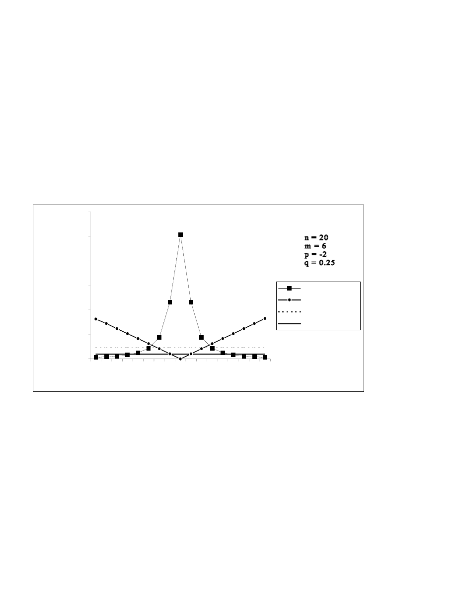
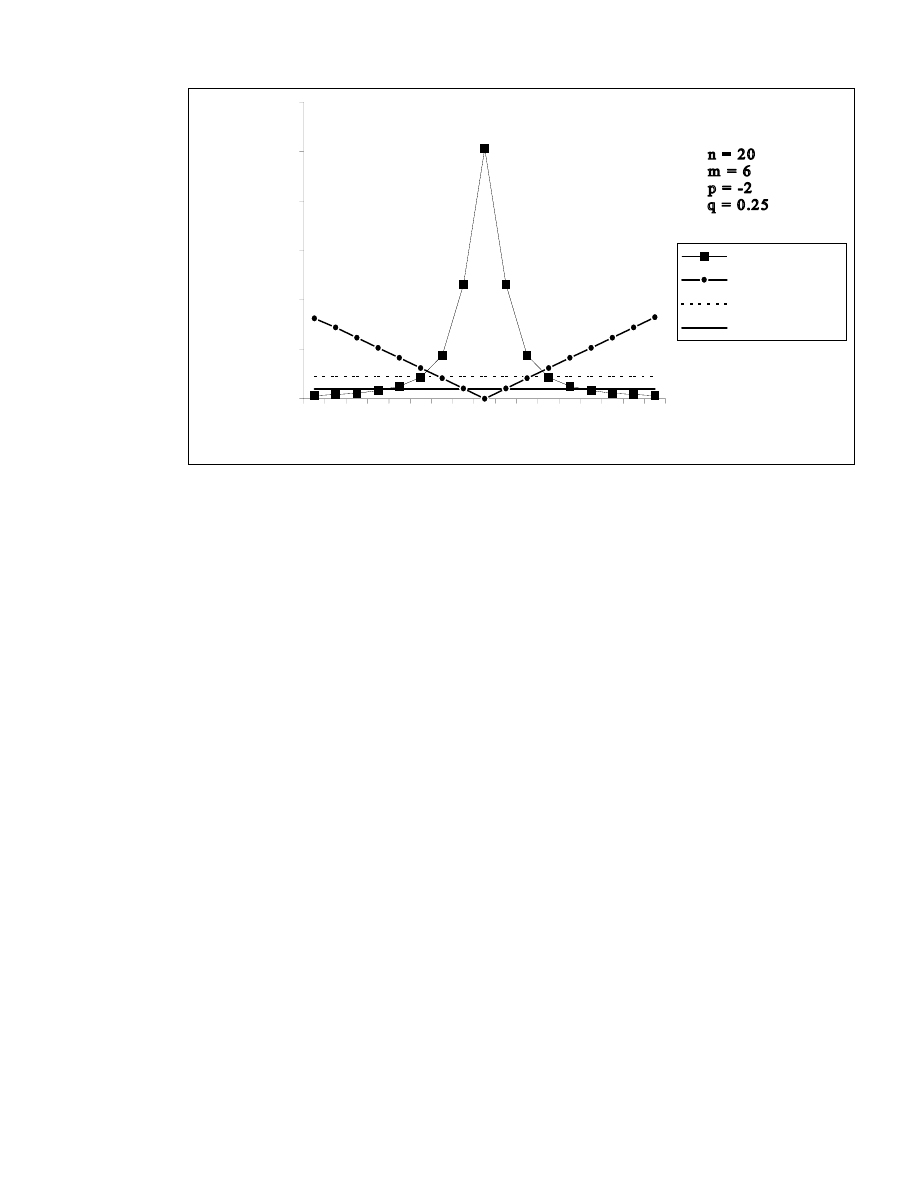
It has been observed from Table 3.1, that on keeping m, p, q fixed, the relative efficiencies of the
proposed class of shrinkage estimators increases up to
∆ = q
−1
, attains its maximum at this point and then
decreases symmetrically in magnitude, as
∆ increases in its range of dominance for all n, p and q. On the
other hand, the ARBs of the proposed class of estimators decreases up to
∆ = q
−1
, the estimator becomes
unbiased at this point and then ARBs increases symmetrically in magnitude, as
∆ increases in its range of
dominance. Thus it is interesting to note that, at q =
∆
−1
, the proposed class of estimators is unbiased with
largest efficiency and hence in the vicinity of q =
∆
−1
also, the proposed class not only renders the massive
gain in efficiency but also it is marginally biased in comparison of MMSE estimator. This implies that q
plays an important role in the proposed class of estimators. The following figure illustrates the discussion.
Figure 3.1
The effect of change in censored sample size m is also a matter of great interest. For fixed p, q and
∆
, the gain in relative efficiency diminishes, and ARB also decreases, with increment in m. Moreover, it
appears that to get better estimators in the class, the value of w(p) should be as small as possible in the
interval (0,1]. Thus, to choose p one should not consider the smaller values of w(p) in isolation, but also the
wider length of the interval of
∆.
0.00
500.00
1000.00
1500.00
2000.00
2500.00
3000.00
0.05
1
2
3
4
5
6
7
8
∆
PRE / ARB*1000
PRE
ARB*1000
ARB(MMSE Esti.)
PRE Cut-off Point

19
4. MODIFIED CLASS OF SHRINKAGE ESTIMATORS AND ITS PROPERTIES
The proposed class of estimators
)
,
(
ˆ
q
p
β
is not uniformly better than
βˆ
. It will be better if
1
β
and
2
β
are in the vicinity of true value
β
. Thus, the centre of the guessed interval
(
)
2
/
2
1
β
+
β
is of much
importance in this case. If we partially violate this, i.e., only the centre of the guessed interval is not of
much importance, but the end points of the interval
1
β
and
2
β
are itself equally important then we can
propose a new class of shrinkage estimators for the shape parameter
β
by using the suggested class
)
,
(
ˆ
q
p
β
as
[
]
{
}
[
]
[
]
[
]
β
−
<
β
β
−
≤
≤
β
−
−
β
+
β
+
−
β
−
>
β
=
β
2
2
1
2
2
1
1
1
)
,
(
)
2
(
if
,
)
2
(
)
2
(
if
,
)
(
1
2
)
(
2
)
2
(
if
,
~
h
t
h
t
h
p
w
q
p
w
t
h
h
t
q
p
(4.1)
which has
{ }
{
}
−
η
∆
+
η
−
η
−
∆
+
−
η
−
−
η
+
η
−
∆
β
=
β
1
2
,
2
,
2
,
)
(
1
1
2
,
1
2
,
)
(
2
,
1
~
Bias
2
2
2
1
2
1
1
1
)
,
(
h
I
h
I
h
I
p
w
q
h
I
h
I
p
w
h
I
q
p
(4.2)
and
{ }
(
)
(
)
(
)
{
}
{
}
{
}
{
}
{
}
{
}
−
−
∆
−
η
−
−
η
+
−
−
∆
η
−
η
−
∆
+
−
η
−
−
η
−
−
+
η
−
∆
∆
+
η
−
∆
∆
−
−
∆
β
=
β
1
)
(
1
1
2
,
1
2
,
)
(
2
2
)
(
1
2
,
2
,
)
(
1
2
2
,
2
2
,
4
2
)
(
2
,
2
2
,
2
1
~
MSE
2
1
2
1
2
1
2
2
2
2
1
1
1
2
1
2
)
,
(
p
w
q
h
I
h
I
p
w
p
w
q
h
I
h
I
p
w
q
h
I
h
I
h
h
p
w
h
I
h
I
q
p
(4.3)
where
1
1
1
1
2
−
∆
−
=
η
h
,
1
2
2
1
2
−
∆
−
=
η
h
and
( )
∫
η
−
ω
−
ω
Γ
=
ω
η
0
1
)
(
1
,
du
u
e
I
u
.

20
This modified class of shrinkage estimators is proposed in accordance with Rao(1973) and it
seems to be more realistic than the previous one as it deals with the case where the whole interval is taken
as apriori information.
5. NUMERICAL ILLUSTRATIONS
The percent relative efficiency of the proposed estimator
)
,
(
~
q
p
β
with respect to MMSE
estimator
m
∧
β
has been defined as
PRE
{
}
{ }
{ }
100
~
MSE
ˆ
MSE
ˆ
,
~
)
,
(
)
,
(
×
β
β
=
β
β
q
p
m
m
q
p
(5.1)
and it is obtained for n = 20 and different values of p, q, m,
1
∆
and
2
∆
(or
∆
). The findings are
summarised in Table 5.1 with corresponding values of h and w(p).
Table 5.1
PREs of proposed estimator
)
,
(
~
q
p
β
with respect to MMSE estimator
m
∧
β
n = 20
p
→
-1
1
m
→
6 8 10 12 6 8 10 12
h
→
10.8519 15.6740 20.8442 26.4026 10.8519 15.6740 20.8442 26.4026
q
↓
∆
1
↓
∆
2
↓
∆↓ w(p)→ 0.7739 0.8537 0.8939 0.9180 0.6888 0.7737 0.8251 0.8779
0.2 0.3
0.25
50.80 41.39 34.91 30.59 49.84 40.10 34.66 31.15
0.4 0.6
0.50
117.60 81.01 67.45 63.17 113.90 79.57 65.63 61.55
0.6 0.9
0.75
261.72 227.42 203.08 172.06 227.59 191.97 172.31 156.69
0.25 0.8 1.2
1.00
548.60 426.98 342.54 286.06 454.93 355.31 293.42 262.79
1.0 1.5
1.25
649.95 470.44 375.91 314.98 636.21 504.49 427.74 353.74
1.2 1.8
1.50
268.31 189.82 150.17 125.21 286.06 210.91 168.38 135.01
1.5 2.0
1.75
80.46 53.66 39.90 31.38 82.35 55.10 40.79 31.74
0.2 0.3
0.25
50.84 41.32 34.76 30.39 49.90 40.03 34.45 30.87
0.4 0.6
0.50
120.81 82.01 67.97 63.49 118.31 81.13 66.48 62.03
0.6 0.9
0.75
298.17 253.12 221.74 184.38 271.73 225.47 198.40 173.57
0.50 0.8 1.2
1.00
642.86 473.19 368.65 303.15 583.65 433.16 344.05 292.64
1.0 1.5
1.25
626.09 435.87 345.16 289.53 658.77 481.87 390.95 317.87
1.2 1.8
1.50
247.90 175.97 140.57 118.43 264.16 191.09 152.66 124.73
1.5 2.0
1.75
78.41 52.66 39.39 31.11 79.96 53.72 40.02 31.36
0.2 0.3
0.25
50.89 41.24 34.60 30.19 49.97 39.95 34.23 30.59
0.4 0.6
0.50
124.02 83.01 68.50 63.81 122.74 82.68 67.32 62.50
0.6 0.9
0.75
339.92 282.24 242.46 197.73 325.66 266.36 229.58 192.68
0.75 0.8 1.2
1.00
723.50 510.42 389.34 316.87 710.96 504.67 388.35 317.53
1.0 1.5
1.25
566.19 392.47 312.16 263.77 597.64 421.61 337.17 278.26

21
1.2 1.8
1.50
224.67 161.95 131.14 111.81 233.41 169.19 136.65 114.63
1.5 2.0
1.75
76.05 51.59 38.85 30.83 76.93 52.14 39.17 30.95

22
Table 5.1 continued …
p
→
-2
2
m
→
6 8 10 12 6 8 10 12
h
→
10.8519 15.6740 20.8442 26.4026 10.8519 15.6740 20.8442 26.4026
q
↓
∆
1
↓
∆
2
↓
∆↓ w(p)→ 0.7739 0.8537 0.8939 0.9180 0.6888 0.7737 0.8251 0.8779
0.2 0.3
0.25
46.04 34.18 30.92 30.53 46.77 34.81 30.96 31.23
0.4 0.6
0.50
92.48 72.59 59.44 53.42 98.00 73.36 59.48 54.88
0.6 0.9
0.75
106.83 95.44 92.75 90.11 128.68 102.24 93.16 100.45
0.25 0.8 1.2
1.00
145.02 131.16 126.15 122.15 191.47 145.23 126.97 144.22
1.0 1.5
1.25
220.29 243.10 282.54 320.74 305.32 273.81 284.60 368.42
1.2 1.8
1.50
208.14 211.32 202.36 179.81 250.20 220.57 202.56 175.49
1.5 2.0
1.75
82.08 57.89 43.07 33.36 84.21 57.95 43.06 33.12
0.2 0.3
0.25
46.28 34.31 30.86 30.24 46.95 34.91 30.90 30.87
0.4 0.6
0.50
103.18 76.82 61.54 54.80 107.21 77.31 61.57 56.08
0.6 0.9
0.75
157.81 135.64 127.02 118.59 181.60 142.94 127.44 128.23
0.50 0.8 1.2
1.00
267.16 228.67 207.62 190.69 331.58 246.71 208.58 212.20
1.0 1.5
1.25
445.44 443.06 448.55 438.38 541.60 467.49 449.42 432.21
1.2 1.8
1.50
289.70 240.03 198.56 163.98 298.93 238.16 198.30 156.40
1.5 2.0
1.75
84.92 57.28 42.13 32.67 84.44 57.03 42.12 32.44
0.2 0.3
0.25
46.50 34.43 30.78 29.92 47.13 34.99 30.82 30.50
0.4 0.6
0.50
114.64 81.04 63.59 56.13 116.87 81.23 63.61 57.24
0.6 0.9
0.75
247.11 202.90 181.31 160.85 266.60 209.00 181.65 167.34
0.75 0.8 1.2
1.00
543.26 418.40 345.15 293.90 596.79 430.93 345.67 302.22
1.0 1.5
1.25
704.42 541.77 447.06 381.03 696.36 532.12 446.25 358.48
1.2 1.8
1.50
280.39 203.46 160.74 132.95 269.47 199.82 160.55 129.07
1.5 2.0
1.75
81.39 54.49 40.40 31.66 80.35 54.26 40.39 31.52
It has been observed from Table 5.1 that likewise
)
,
(
ˆ
q
p
β
the PRE of
)
,
(
~
q
p
β
with respect to
m
βˆ
decreases as censoring fraction (m/n) increases. For fixed m, p and q the relative efficiency increases up to
a certain point of
∆
, procures its maximum at this point and then starts decreasing as
∆
increases. It
seems from the expression in (4.3) that the point of maximum efficiency may be a point where either any
one of the following holds or any two of the following holds or all the following three holds-
(i)
the lower end point of the guessed interval, i.e.,
1
β
coincides exactly with the true value
β
, i.e.,
1
∆
= 1.
(ii)
the upper end point of the guessed interval, i.e.,
2
β
departs exactly two times from the true value
β
, i.e.,
2
∆
= 2.
(iii)
1
−
=
∆ q
This leads to say that on contrary to
)
,
(
ˆ
q
p
β
, there is much importance of
1
∆
and
2
∆
in addition to
∆
.
The discussion is also supported by the illustrations in Table 5.1. As well, the range of dominance of

23
average departure
∆
is smaller than that is obtained for
)
,
(
ˆ
q
p
β
but this does not humiliate the merit of
)
,
(
~
q
p
β
because still the range of dominance of
∆
is enough wider.
6. CONCLUSION AND RECOMMENDATIONS
It has been seen that the suggested classes of shrunken estimators have considerable gain in
efficiency for a number of choices of scalars comprehend in it, particularly for heavily censored samples,
i.e., for small m. Even for buoyantly censored samples, i.e., for large m, so far as the proper selection of
scalars is concerned, some of the estimators from the suggested classes of shrinkage estimators are more
efficient than the MMSE estimators subject to certain conditions. Accordingly, even if the experimenter has
less confidence in the guessed interval
(
)
2
1
,
β
β
of
β, the efficiency of the suggested classes of shrinkage
estimators can be increased considerably by choosing the scalars p and q appropriately.
While dealing with the suggested class of shrunken estimators
)
,
(
ˆ
q
p
β
it is recommended that one
should not consider the substantial gain in efficiency in isolation, but also the wider range of dominance of
∆
, because enough flexible range of dominance of
∆
will leads to increase the possibility of getting
better estimators from the proposed class. Thus it is recommended to use the proposed class of shrunken
estimators in practice.
REFERENCES
BAIN, L. J. (1972) : Inferences based on Censored Sampling from the Weibull or Extreme-value
distribution, Technometrics, 14, 693-703.
BERRETTONI, J. N. (1964) : Practical Applications of the Weibull distribution, Industrial Quality
Control, 21, 71-79.
ENGELHARDT, M. and BAIN, L. J. (1973) : Some Complete and Censored Sampling Results for the
Weibull or Extreme-value distribution, Technometrics, 15, 541-549.
ENGELHARDT, M. (1975) : On Simple Estimation of the Parameters of the Weibull or Extreme-value
distribution, Technometrics, 17, 369-374.
JAMES, W. and STEIN, C. (1961) : (A basic paper on Stein-type estimators), Proceedings of the 4
th
Berkeley Symposium on Mathematical Statistics, Vol. 1, University of California Press, Berkeley, CA,
361-379.
KAO, J. H. K. (1958) : Computer Methods for estimating Weibull parameters in Reliability Studies,
Transactions of IRE-Reliability and Quality Control, 13, 15-22.

24
KAO, J. H. K. (1959) : A Graphical Estimation of Mixed Weibull parameters in Life-testing Electron
Tubes, Technometrics, 1, 389-407.
LIEBLEIN, J. and ZELEN, M. (1956) : Statistical Investigation of the Fatigue Life of Deep Groove Ball
Bearings, Journal of Res. Natl. Bur. Std., 57, 273-315.
MANN, N. R. (1967 A) : Results on Location and Scale Parameter Estimation with Application to the
Extreme-value distribution, Aerospace Research Labs, Wright Patterson AFB, AD.653575, ARL-67-0023.
MANN, N. R. (1967 B) : Table for obtaining Best Linear Invariant estimates of parameters of Weibull
distribution, Technometrics, 9, 629-645.
MANN, N. R. (1968 A) : Results on Statistical Estimation and Hypothesis Testing with Application to the
Weibull and Extreme Value Distribution, Aerospace Research Laboratories, Wright-Patterson Air Force
Base, Ohio.
MANN, N. R. (1968 B) : Point and Interval Estimation for the Two-parameter Weibull and Extreme-value
distribution, Technometrics, 10, 231-256.
PANDEY, M. (1983) : Shrunken estimators of Weibull shape parameters in censored samples, IEEE Trans.
Reliability, R-32, 200-203.
PANDEY, M. and UPADHYAY, S. K. (1985) : Bayesian Shrinkage estimation of Weibull parameters,
IEEE Transactions on Reliability, R-34, 491-494.
PANDEY, M. and UPADHYAY, S. K. (1986) : Selection based on modified Likelihood Ratio and
Adaptive estimation from a Censored Sample, Jour. Indian Statist. Association, 24, 43-52.
RAO, C. R. (1973) : Linear Statistical Inference and its Applications, Sankhya, Ser. B, 39, 382-393.
SINGH, H. P. and SHUKLA, S. K. (2000) : Estimation in the Two-parameter Weibull distribution with
Prior Information, IAPQR Transactions, 25, 2, 107-118.
SINGH, J. and BHATKULIKAR, S. G. (1978) :Shrunken estimation in Weibull distribution, Sankhya, 39,
382-393.
THOMPSON, J. R. (1968 A) : Some Shrinkage Techniques for Estimating the Mean, The Journal of
American Statistical Association, 63, 113-123.
THOMPSON, J. R. (1968 B) : Accuracy borrowing in the Estimation of the Mean by Shrinkage to an
Interval , The Journal of American Statistical Association, 63, 953-963.
WEIBULL, W. (1939) : The phenomenon of Rupture in Solids, Ingenior Vetenskaps Akademiens
Handlingar, 153,2.
WEIBULL, W. (1951) : A Statistical distribution function of wide Applicability, Journal of Applied
Mechanics, 18, 293-297.

25
WHITE, J. S. (1969) : The moments of log-Weibull order Statistics, Technometrics,11, 373-386.

26
A General Class of Estimators of Population Median Using Two Auxiliary
Variables in Double Sampling
Mohammad Khoshnevisan
1
, Housila P. Singh
2
, Sarjinder Singh
3
, Florentin
Smarandache
4
1
School of Accounting and Finance, Griffith University, Australia
2
School of Studies in Statistics, Vikram University, Ujjain - 456 010 (M. P.), India
3
Department of Mathematics and Statistics, University of Saskatchewan, Canada
4
Department of Mathematics, University of New Mexico, Gallup, USA
Abstract:
In this paper we have suggested two classes of estimators for population median M
Y
of the study character
Y using information on two auxiliary characters X and Z in double sampling. It has been shown that the
suggested classes of estimators are more efficient than the one suggested by Singh et al (2001). Estimators
based on estimated optimum values have been also considered with their properties. The optimum values
of the first phase and second phase sample sizes are also obtained for the fixed cost of survey.
Keywords: Median estimation, Chain ratio and regression estimators, Study variate, Auxiliary variate,
Classes of estimators, Mean squared errors, Cost, Double sampling.
2000 MSC: 60E99
1. INTRODUCTION
In survey sampling, statisticians often come across the study of variables which have highly skewed
distributions, such as income, expenditure etc. In such situations, the estimation of median deserves special
attention. Kuk and Mak (1989) are the first to introduce the estimation of population median of the study
variate Y using auxiliary information in survey sampling. Francisco and Fuller (1991) have also
considered the problem of estimation of the median as part of the estimation of a finite population
distribution function. Later Singh et al (2001) have dealt extensively with the problem of estimation of
median using auxiliary information on an auxiliary variate in two phase sampling.
Consider a finite population U={1,2,
…,i,...,N}. Let Y and X be the variable for study and auxiliary
variable, taking values Y
i
and X
i
respectively for the i-th unit. When the two variables are strongly related
but no information is available on the population median M
X
of X, we seek to estimate the population
median M
Y
of Y from a sample S
m
, obtained through a two-phase selection. Permitting simple random
sampling without replacement (SRSWOR) design in each phase, the two-phase sampling scheme will be as
follows:
(i)
The first phase sample S
n
(S
n
⊂U) of fixed size n is drawn to observe only X in order to
furnish an estimate of M
X
.
(ii)
Given
S
n
, the second phase sample S
m
(S
m
⊂S
n
) of fixed size m is drawn to observe Y
only.
Assuming that the median M
X
of the variable X is known, Kuk and Mak (1989) suggested a ratio estimator
for the population median M
Y
of Y as

27
X
X
Y
M
M
M
M
ˆ
ˆ
ˆ
1
=
(1.1)
where
Y
Mˆ
and
X
Mˆ
are the sample estimators of M
Y
and M
X
respectively based on a sample S
m
of size
m. Suppose that y
(1)
, y
(2)
,
…, y
(m)
are the y values of sample units in ascending order. Further, let t be an
integer such that Y
(t)
≤ M
Y
≤Y
(t+1)
and let p=t/m be the proportion of Y, values in the sample that are less
than or equal to the median value M
Y
, an unknown population parameter. If
pˆ
is a predictor of p, the
sample median
Y
Mˆ
can be written in terms of quantities as
( )
p
Q
Y
ˆ
ˆ
where
5
.
0
ˆ
=
p
. Kuk and Mak
(1989) define a matrix of proportions (P
ij
(x,y)) as
Y
≤ M
Y
Y > M
Y
Total
X
≤ M
X
P
11
(x,y) P
21
(x,y)
P
⋅1
(x,y)
X > M
X
P
12
(x,y) P
22
(x,y)
P
⋅2
(x,y)
Total
P
1
⋅(x,y) P
2
⋅(x,y)
1
and a position estimator of M
y
given by
( )
( )
Y
Y
p
Y
p
Q
M
ˆ
ˆ
ˆ
=
(1.2)
−
+
≈
−
+
=
⋅
⋅
m
y
x
p
m
m
y
x
p
m
y
x
p
y
x
p
m
m
y
x
p
y
x
p
m
m
p
x
x
x
x
Y
)
,
(
ˆ
)
(
)
,
(
ˆ
2
)
,
(
ˆ
)
,
(
ˆ
)
(
)
,
(
ˆ
)
,
(
ˆ
1
ˆ
where
12
11
2
12
1
11
with
)
,
(
ˆ
y
x
p
ij
being the sample analogues of the P
ij
(x,y) obtained from the population and m
x
the number
of units in S
m
with X
≤ M
X
.
Let
)
(
~
y
F
YA
and
)
(
~
y
F
YB
denote the proportion of units in the sample S
m
with X
≤ M
X
, and X>M
X
,
respectively that have Y values less than or equal to y. Then for estimating M
Y
, Kuk and Mak (1989)
suggested the 'stratification estimator' as
( )
{
}
5
.
0
~
:
inf
ˆ
)
(
≥
=
y
Y
St
Y
F
y
M
(1.3)
where
[
]
)
(
)
(
~
~
2
1
)
(
ˆ
y
YB
y
YA
Y
F
F
y
F
+
≅
It is to be noted that the estimators defined in (1.1), (1.2) and (1.3) are based on prior knowledge of the
median M
X
of the auxiliary character X. In many situations of practical importance the population median
M
X
of X may not be known. This led Singh et al (2001) to discuss the problem of estimating the
population median M
Y
in double sampling and suggested an analogous ratio estimator as
X
X
Y
d
M
M
M
M
ˆ
ˆ
ˆ
ˆ
1
1
=
(1.4)

28
where
1
ˆ
X
M
is sample median based on first phase sample S
n
.
Sometimes even if M
X
is unknown, information on a second auxiliary variable Z, closely related to X but
compared X remotely related to Y, is available on all units of the population. This type of situation has
been briefly discussed by, among others, Chand (1975), Kiregyera (1980, 84), Srivenkataramana and Tracy
(1989), Sahoo and Sahoo (1993) and Singh (1993). Let M
Z
be the known population median of Z.
Defining
−
=
−
−
=
−
=
−
=
1
M
M
ˆ
e
and
1
ˆ
,
1
ˆ
,
1
ˆ
,
1
ˆ
Z
1
Z
4
3
1
2
1
0
Z
Z
X
X
X
X
Y
Y
M
M
e
M
M
e
M
M
e
M
M
e
such that E(e
k
)
≅0 and e
k
<1 for k=0,1,2,3; where
2
ˆ
M
and
1
2
ˆ
M
are the sample median estimators based
on second phase sample S
m
and first phase sample S
n
. Let us define the following two new matrices as
Z
≤ M
Z
Z > M
Z
Total
X
≤ M
X
P
11
(x,z) P
21
(x,z)
P
⋅1
(x,z)
X > M
X
P
12
(x,z) P
22
(x,z)
P
⋅2
(x,z)
Total
P
1
⋅(x,z) P
2
⋅(x,z)
1
and
Z
≤ M
Z
Z > M
Z
Total
Y
≤ M
Y
P
11
(y,z) P
21
(y,z)
P
⋅1
(y,z)
Y > M
Y
P
12
(y,z) P
22
(y,z)
P
⋅2
(y,z)
Total
P
1
⋅(y,z) P
2
⋅(y,z)
1
Using results given in the Appendix-1, to the first order of approximation, we have
E(e
0
2
) =
N-m
N (4m)
-1
{M
Y
f
Y
(M
Y
)}
-2
,
E(e
1
2
) =
N-m
N (4m)
-1
{M
X
f
X
(M
X
)}
-2
,
E(e
2
2
) =
N-n
N (4n)
-1
{M
X
f
X
(M
X
)}
-2
,
E(e
3
2
) =
N-m
N (4m)
-1
{M
Z
f
Z
(M
Z
)}
-2
,
E(e
4
2
) =
N-n
N (4n)
-1
{M
Z
f
Z
(M
Z
)}
-2
,
E(e
0
e
1
) =
N-m
N (4m)
-1
{4P
11
(x,y)-1}{M
X
M
Y
f
X
(M
X
)f
Y
(M
Y
)}
-1
,
E(e
0
e
2
) =
N-n
N (4n)
-1
{4P
11
(x,y)-1}{M
X
M
Y
f
X
(M
X
)f
Y
(M
Y
)}
-1
,
E(e
0
e
3
) =
N-m
N (4m)
-1
{4P
11
(y,z)-1}{M
Y
M
Z
f
Y
(M
Y
)f
Z
(M
Z
)}
-1
,
E(e
0
e
4
) =
N-n
N (4n)
-1
{4P
11
(y,z)-1}{M
Y
M
Z
f
Y
(M
Y
)f
Z
(M
Z
)}
-1
,
E(e
1
e
2
) =
N-n
N (4n)
-1
{M
X
f
X
(M
X
)}
-2
,
E(e
1
e
3
) =
N-m
N (4m)
-1
{4P
11
(x,z)-1}{M
X
M
Z
f
X
(M
X
)f
Z
(M
Z
)}
-1
,

29
E(e
1
e
4
) =
N-n
N (4n)
-1
{4P
11
(x,z)-1}{M
X
M
Z
f
X
(M
X
)f
Z
(M
Z
)}
-1
,
E(e
2
e
3
) =
N-n
N (4n)
-1
{4P
11
(x,z)-1}{M
X
M
Z
f
X
(M
X
)f
Z
(M
Z
)}
-1
,
E(e
2
e
4
) =
N-n
N (4n)
-1
{4P
11
(x,z)-1}{M
X
M
Z
f
X
(M
X
)f
Z
(M
Z
)}
-1
,
E(e
3
e
4
) =
N-n
N (4n)
-1
(f
Z
(M
Z
)M
Z
)
-2
where it is assumed that as N
→∞ the distribution of the trivariate variable (X,Y,Z) approaches a continuous
distribution with marginal densities f
X
(x), f
Y
(y) and f
Z
(z) for X, Y and Z respectively. This assumption
holds in particular under a superpopulation model framework, treating the values of (X, Y, Z) in the
population as a realization of N independent observations from a continuous distribution. We also assume
that f
Y
(M
Y
), f
X
(M
X
) and f
Z
(M
Z
) are positive.
Under these conditions, the sample median
Y
Mˆ
is consistent and asymptotically normal (Gross, 1980) with
mean M
Y
and variance
( )
( )
{
}
2
1
4
−
−
−
Y
Y
M
f
m
N
m
N
In this paper we have suggested a class of estimators for M
Y
using information on two auxiliary variables X
and Z in double sampling and analyzes its properties.
2. SUGGESTED CLASS OF ESTIMATORS
Motivated by Srivastava (1971), we suggest a class of estimators of M
Y
of Y as
( )
( )
( )
{
}
v
u
g
M
M
M
g
Y
g
Y
g
Y
,
ˆ
:
ˆ
=
=
(2.1)
where
Z
Z
X
X
M
M
v
M
M
u
ˆ
ˆ
,
ˆ
ˆ
1
1
=
=
and g(u,v) is a function of u and v such that g(1,1)=1 and such that it satisfies
the following conditions.
1.
Whatever be the samples (S
n
and S
m
) chosen, let (u,v) assume values in a closed convex sub-
space, P, of the two dimensional real space containing the point (1,1).
2.
The function g(u,v) is continuous in P, such that g(1,1)=1.
3.
The first and second order partial derivatives of g(u,v) exist and are also continuous in P.
Expanding g(u,v) about the point (1,1) in a second order Taylor's series and taking expectations, it is found
that
( )
(
)
)
(
0
ˆ
1
−
+
=
n
M
M
E
Y
g
Y
so the bias is of order n
−1
.
Using a first order Taylor's series expansion around the point (1,1) and noting that g(1,1)=1, we have

30
( )
(
) ( )
( )
( )
]
0
1
,
1
1
,
1
1
[
ˆ
1
2
4
1
2
1
0
−
+
+
−
+
+
≅
n
g
e
g
e
e
e
M
M
Y
g
Y
or
( )
(
)
(
) ( )
( )
[
]
1
,
1
1
,
1
2
4
1
2
1
0
g
e
g
e
e
e
M
M
M
Y
Y
g
Y
+
−
+
≅
−
(2.2)
where g
1
(1,1) and g
2
(1,1) denote first order partial derivatives of g(u,v) with respect to u and v respectively
around the point (1,1).
Squaring both sides in (2.2) and then taking expectations, we get the variance of
)
(
ˆ
g
Y
M
to the first degree
of approximation, as
( )
(
)
( )
(
)
,
1
1
1
1
1
1
4
1
ˆ
2
−
+
−
+
−
=
B
N
n
A
n
m
N
m
M
f
M
Var
Y
Y
g
Y
(2.3)
where
( )
(
)
( )
(
) ( )
( )
(
)
−
+
=
1
,
4
2
1
,
1
)
1
,
1
(
11
1
1
y
x
P
g
M
f
M
M
f
M
g
M
f
M
M
f
M
A
X
X
X
Y
Y
Y
X
X
X
Y
Y
Y
(2.4)
( )
(
)
( )
( )
(
) ( )
( )
(
)
−
+
=
1
,
4
2
1
,
1
1
,
1
11
2
z
y
P
g
M
f
M
M
f
M
g
M
f
M
M
f
M
B
Z
Z
Z
Y
Y
Y
Z
Z
Z
Z
Y
Y
Y
(2.5)
The variance of
( )
g
Y
Mˆ
in (2.3) is minimized for
(
)
( )
( )
(
)
(
)
( )
( )
(
)
1
,
4
)
1
,
1
(
1
,
4
)
1
,
1
(
11
2
11
1
−
−
=
−
−
=
z
y
P
M
f
M
M
f
M
g
y
x
P
M
f
M
M
f
M
g
Y
Y
Y
Z
Z
Z
Y
Y
Y
X
X
X
(2.6)
Thus the resulting (minimum) variance of
( )
g
Y
M
is given by
( )
(
)
( )
(
)
( )
(
)
( )
(
)
−
−
−
−
−
−
−
=
1
,
4
1
1
1
,
4
1
1
1
1
4
1
ˆ
Var
min.
11
2
11
2
z
y
P
N
n
y
x
P
n
m
N
m
M
f
M
Y
Y
g
Y
(2.7)
Now, we proved the following theorem.
Theorem 2.1 - Up to terms of order n
-1
,
( )
( )
(
)
( )
(
)
( )
(
)
−
−
−
−
−
−
−
≥
2
11
2
11
2
Y
1
,
4
1
1
1
,
4
1
1
1
1
4
1
M
ˆ
Var
z
y
P
N
n
y
x
P
n
m
N
m
M
f
Y
y
g
with equality holding if

31
( )
( )
( )
(
)
( )
( )
( )
(
)
1
,
4
)
1
,
1
(
1
,
4
)
1
,
1
(
11
2
11
1
−
−
=
−
−
=
z
y
P
M
f
M
M
f
M
g
y
x
P
M
f
M
M
f
M
g
Y
Y
Y
z
z
z
Y
Y
Y
x
x
x
It is interesting to note that the lower bound of the variance of
( )
g
y
Mˆ
at (2.1) is the variance of the linear
regression estimator
( )
(
) (
)
1
2
1
1
ˆ
ˆ
ˆ
ˆ
ˆ
ˆ
ˆ
Z
Z
X
X
Y
l
Y
M
M
d
M
M
d
M
M
−
+
−
+
=
(2.8)
where
( )
( )
( )
(
)
( )
( )
( )
(
)
,
1
,
ˆ
4
ˆ
ˆ
ˆ
ˆ
ˆ
,
1
,
ˆ
4
ˆ
ˆ
ˆ
ˆ
ˆ
11
2
11
1
−
=
−
=
z
y
p
M
f
M
f
d
y
x
p
M
f
M
f
d
Y
Y
Z
Z
y
Y
x
X
with
( )
y
x
p
,
ˆ
11
and
( )
z
y
p
,
ˆ
11
being the sample analogues of the
( )
y
x
p
,
11
and
( )
z
y
p
,
11
respectively
and
( )
(
)
X
X
Y
Y
M
f
M
f
ˆ
,
ˆ
ˆ
and
( )
Z
Z
M
fˆ
can be obtained by following Silverman (1986).
Any parametric function g(u,v) satisfying the conditions (1), (2) and (3) can generate an asymptotically
acceptable estimator. The class of such estimators are large. The following simple functions g(u,v) give
even estimators of the class
( )
( )
( )
( )
(
)
(
)
,
1
1
1
1
,
,
,
2
1
−
−
−
+
=
=
v
u
v
u
g
v
u
v
u
g
β
α
β
α
( )
( )
(
) (
)
( )
( )
(
) (
)
{
}
1
4
3
1
1
1
,
,
1
1
1
,
−
−
−
−
−
=
−
+
−
+
=
v
u
v
u
g
v
u
v
u
g
β
α
β
α
( )
( )
1
,
,
2
1
2
1
5
=
+
+
=
w
w
v
w
u
w
v
u
g
β
α
( )
( )
(
)
( )
( )
(
) (
)
{
}
1
1
exp
,
,
1
,
7
6
−
+
−
=
−
+
=
v
u
v
u
g
v
u
v
u
g
β
α
α
α
β
Let the seven estimators generated by g
(i)
(u,v) be denoted by
( )
( )
( ) (
)
7
to
1
,
,
ˆ
ˆ
=
=
i
v
u
g
M
M
i
Y
g
Yi
. It is
easily seen that the optimum values of the parameters
α,β,w
i
(i-1,2) are given by the right hand sides of
(2.6).
3. A WIDER CLASS OF ESTIMATORS
The class of estimators (2.1) does not include the estimator
(
) (
)
(
)
2
1
1
2
1
1
,
,
ˆ
ˆ
ˆ
ˆ
d
d
M
M
d
M
M
d
M
M
Z
Z
X
X
Y
Yd
−
+
−
+
=
being constants.

32
However, it is easily shown that if we consider a class of estimators wider than (2.1), defined by
( )
(
)
v
u
M
G
M
Y
G
Y
,
,
ˆ
ˆ
1
=
(3.1)
of M
Y
, where G(
⋅) is a function of
Y
Mˆ
, u and v such that
(
)
Y
Y
M
M
G
=
1
,
1
,
and
(
)
1
1
,
1
,
1
=
Y
M
G
.
(
)
1
,
1
,
1
Y
M
G
denoting the first partial derivative of G(
⋅) with respect to
Y
Mˆ
.
Proceeding as in Section 2 it is easily seen that the bias of
( )
G
Y
Mˆ
is of the order n
−1
and up to this order of
terms, the variance of
( )
G
Y
Mˆ
is given by
( )
(
)
( )
(
)
( )
(
)
(
)
( )
(
)
(
)
( )
(
)
( )
( )
( )
( )
(
)
( )
(
)
]
1
,
4
2
1
,
1
,
1
1
1
,
4
2
1
,
1
,
1
,
1
,
1
1
1
1
[
4
1
M
ˆ
Var
11
3
11
2
2
2
Y
−
+
−
+
−
+
−
+
−
=
z
y
P
M
G
M
f
M
M
f
M
M
f
M
f
N
n
y
x
P
M
G
M
f
M
M
f
M
G
M
f
M
M
f
n
m
N
m
M
f
Y
Z
Z
Z
Y
Y
Z
Z
Z
Y
Y
Y
X
X
X
Y
Y
Y
X
X
X
Y
Y
Y
Y
G
(3.2)
where G
2
(M
Y
1,1) and G
3
(M
Y
1,1) denote the first partial derivatives of u and v respectively around the point
(M
Y
,(1,1).
The variance of
( )
G
Y
Mˆ
is minimized for
(
)
(
)
( )
( )
(
)
(
)
( )
( )
( )
(
)
1
,
4
1
,
1
,
1
,
4
1
,
1
,
11
3
11
2
−
−
=
−
−
=
z
y
P
M
f
M
f
M
M
G
y
x
P
M
f
M
f
M
M
G
Y
Y
Z
Z
Z
Y
Y
Y
X
X
X
Y
(3.3)
Substitution of (3.3) in (3.2) yields the minimum variance of
( )
G
Y
Mˆ
as
( )
(
)
( )
(
)
( )
(
)
( )
(
)
(
)
)
(
Y
2
11
2
11
2
Y
M
ˆ
min.Var
]
1
,
4
1
1
1
,
4
1
1
1
1
[
4
1
M
ˆ
Var
min.
g
Y
Y
G
z
y
P
N
n
y
x
P
n
m
N
m
M
f
=
−
−
−
−
−
−
−
=
(3.4)
Thus we established the following theorem. Theorem 3.1 - Up to terms of order n
-1
,

33
( )
(
)
( )
(
)
( )
(
)
( )
(
)
−
−
−
−
−
−
−
≥
2
11
2
11
2
Y
1
,
4
1
1
1
,
4
1
1
1
1
4
1
M
ˆ
Var
z
y
P
N
n
y
x
P
n
m
N
m
M
f
Y
Y
G
with equality holding if
(
)
(
)
( )
( )
(
)
(
)
( )
( )
( )
(
)
1
,
4
1
,
1
,
1
,
4
1
,
1
,
11
3
11
2
−
−
=
−
−
=
z
y
P
M
f
M
f
M
M
G
y
x
P
M
f
M
M
f
M
G
Y
Y
Z
Z
Z
Y
Y
Y
X
X
x
Y
If the information on second auxiliary variable z is not used, then the class of estimators
( )
G
Y
Mˆ
reduces to
the class of estimators of M
Y
as
( )
(
)
u
M
H
M
Y
H
Y
,
ˆ
ˆ
=
(3.5)
where
(
)
u
M
H
Y
,
ˆ
is a function of
(
)
u
M
Y
,
ˆ
such that
(
)
Y
Y
M
M
H
=
1
,
and
(
)
,
1
1
,
1
=
Y
M
H
(
)
( )
(
)
1
,
1
ˆ
1
,
Y
M
Y
Y
M
H
M
H
∂
⋅
∂
=
. The estimator
( )
H
Y
Mˆ
is reported by Singh et al (2001).
The minimum variance of
( )
H
Y
Mˆ
to the first degree of approximation is given by
( )
(
)
( )
(
)
( )
(
)
−
−
−
−
=
2
11
2
Y
1
,
4
1
1
1
1
4
1
M
ˆ
min.Var
y
x
P
n
m
N
m
M
f
Y
Y
H
(3.6)
From (3.4) and (3.6) we have
( )
(
)
( )
(
)
( )
(
)
( )
(
)
2
11
2
Y
Y
1
,
4
4
1
1
1
M
ˆ
min.Var
M
ˆ
minVar
−
−
=
−
z
y
P
M
f
N
n
Y
Y
G
H
(3.7)
which is always positive. Thus the proposed class of estimators
( )
G
Y
Mˆ
is more efficient than the estimator
( )
H
Y
Mˆ
considered by Singh et al (2001).
4. ESTIMATOR BASED ON ESTIMATED OPTIMUM VALUES
We denote
(
)
( )
( )
(
)
( )
( )
( )
(
)
1
,
4
1
,
4
11
2
11
1
−
=
−
=
z
y
P
M
f
M
M
f
M
y
x
P
M
f
M
M
f
M
Y
Y
Y
Z
Z
Z
Y
Y
Y
X
X
X
α
α
(4.1)

34
In practice the optimum values of g
1
(1,1)(=-
α
1
) and g
2
(1,1)(=-
α
2
) are not known. Then we use to find out
their sample estimates from the data at hand. Estimators of optimum value of g
1
(1,1) and g
2
(1,1) are given
as
( )
( )
2
2
1
1
ˆ
1
,
1
ˆ
ˆ
1
,
1
ˆ
α
α
−
=
−
=
g
g
(4.2)
where
( )
( )
( )
(
)
( )
( )
( )
(
)
1
,
4
ˆ
ˆ
ˆ
ˆ
ˆ
ˆ
ˆ
1
,
ˆ
4
ˆ
ˆ
ˆ
ˆ
ˆ
ˆ
ˆ
11
2
11
1
−
=
−
=
z
y
p
M
f
M
M
f
M
y
x
p
M
f
M
M
f
M
Y
Y
Y
Z
Z
Z
Y
Y
Y
X
X
X
α
α
(4.3)
Now following the procedure discussed in Singh and Singh (19xx) and Srivastava and Jhajj (1983), we
define the following class of estimators of M
Y
(based on estimated optimum) as
( )
(
)
2
1
*
ˆ
,
ˆ
,
,
*
ˆ
ˆ
α
α
v
u
g
M
M
Y
g
Y
=
(4.4)
where g*(
⋅) is a function of
2
1
ˆ
,
ˆ
,
,
(
α
α
v
u
) such that
(
)
(
)
( )
(
)
(
)
( )
(
)
(
)
( )
(
)
(
)
( )
(
)
0
ˆ
*
,
,
1
,
1
0
ˆ
*
,
,
1
,
1
*
,
,
1
,
1
*
,
,
1
,
1
1
,
1
,
1
*
2
1
2
1
2
1
2
1
,
,
1
,
1
2
2
1
*
4
,
,
1
,
1
1
2
1
*
3
2
,
,
1
,
1
2
1
*
2
1
,
,
1
,
1
2
1
*
1
2
1
=
∂
⋅
∂
=
=
∂
⋅
∂
=
−
=
∂
⋅
∂
=
−
=
∂
⋅
∂
=
=
α
α
α
α
α
α
α
α
α
α
α
α
α
α
α
α
α
α
α
α
α
α
g
g
g
g
v
g
g
u
g
g
g
and such that it satisfies the following conditions:
1.
Whatever be the samples (S
n
and S
m
) chosen, let
2
1
ˆ
ˆ
,
,
α
α
v
u
assume values in a closed convex sub-
space, S, of the four dimensional real space containing the point (1,1,
α
1
,
α
2
).
2.
The function g*(u,v,
α
1
,
α
2
) continuous in S.
3.
The first and second order partial derivatives of
(
)
2
1
ˆ
,
ˆ
,
,
*
α
α
v
u
g
exst. and are also continuous in
S.
Under the above conditions, it can be shown that
( )
(
)
( )
1
*
0
ˆ
−
+
=
n
M
M
E
Y
g
Y

35
and to the first degree of approximation, the variance of
( )
*
ˆ
g
Y
M
is given by
( )
(
)
( )
g
g
Y
M
Y
*
M
ˆ
min.Var
ˆ
Var
=
(4.5)
where
( )
(
)
g
Y
Mˆ
min.Var
is given in (2.7).
A wider class of estimators of M
Y
based on estimated optimum values is defined by
( )
(
)
*
2
*
1
*
ˆ
,
ˆ
,
,
,
ˆ
*
ˆ
α
α
v
u
M
G
M
Y
G
Y
=
(4.6)
where
( )
( )
( )
(
)
( )
( )
( )
(
)
1
,
ˆ
4
ˆ
ˆ
ˆ
ˆ
ˆ
ˆ
1
,
ˆ
4
ˆ
ˆ
ˆ
ˆ
ˆ
ˆ
11
*
2
11
*
1
−
=
−
=
z
y
p
M
f
M
f
M
y
x
p
M
f
M
f
M
Y
Y
Z
Z
Z
Y
Y
X
X
X
α
α
(4.7)
are the estimates of
(
)
( )
( )
(
)
( )
( )
( )
(
)
1
,
4
1
,
4
11
*
2
11
*
1
−
=
−
=
z
y
P
M
f
M
f
M
y
x
P
M
f
M
f
M
Y
Y
Z
Z
Z
Y
Y
X
X
x
α
α
(4.8)
and G*(
⋅) is a function of
(
)
*
2
*
1
ˆ
,
,
,
,
ˆ
α
α
v
u
M
Y
such that
(
)
(
)
( )
(
)
(
)
( )
(
)
*
1
,
,
1
,
1
,
*
2
*
1
*
2
,
,
1
,
1
,
*
2
*
1
*
1
*
2
*
1
*
2
*
1
*
2
*
1
*
,
,
1
,
1
1
ˆ
*
,
,
1
,
1
,
,
,
1
,
1
,
*
α
α
α
α
α
α
α
α
α
α
α
−
=
∂
⋅
∂
=
=
∂
⋅
∂
=
=
Y
Y
M
Y
M
Y
Y
Y
Y
u
G
M
G
M
G
M
G
M
M
G
(
)
( )
(
)
*
2
,
1
,
1
*
2
*
1
*
3
*
2
*,
1
*
,
,
1
,
1
α
α
α
α
−
=
∂
⋅
∂
=
∂
Y
M
Y
v
G
M
G
(
)
( )
(
)
0
ˆ
*
,
,
1
,
1
*
2
*
1
,
,
1
,
1
,
*
1
*
2
*
1
*
4
=
∂
⋅
∂
=
α
α
α
α
α
Y
M
Y
G
M
G

36
(
)
( )
(
)
0
ˆ
*
,
,
1
,
1
*
2
*
1
,
,
1
,
1
,
*
2
*
2
*
1
*
5
=
∂
⋅
∂
=
α
α
α
α
α
Y
M
Y
G
M
G
Under these conditions it can be easily shown that
( )
(
)
( )
1
*
0
ˆ
−
+
=
n
M
M
E
Y
G
Y
and to the first degree of approximation, the variance of
( )
*
ˆ
G
Y
M
is given by
(
)
( )
(
)
G
Y
G
Y
M
M
ˆ
min.Var
ˆ
Var
*
=
(4.9)
where
( )
G
Y
Mˆ
min.Var
is given in (3.4).
It is to be mentioned that a large number of estimators can be generated from the classes
( )
*
ˆ
g
Y
M
and
( )
*
ˆ
G
Y
M
based on estimated optimum values.
5. EFFICIENCY OF THE SUGGESTED CLASS OF ESTIMATORS FOR FIXED COST
The appropriate estimator based on on single-phase sampling without using any auxiliary variable is
Y
Mˆ
,
whose variance is given by
( )
( )
(
)
2
4
1
1
1
ˆ
Var
Y
Y
Y
M
f
N
m
M
−
=
(5.1)
In case when we do not use any auxiliary character then the cost function is of the form C
0
-mC
1
, where C
0
and C
1
are total cost and cost per unit of collecting information on the character Y.
The optimum value of the variance for the fixed cost C
0
is given by
( )
−
=
N
C
G
V
M
Y
1
ˆ
Var
.
Opt
0
0
(5.2)
where
( )
(
)
2
0
4
1
Y
Y
M
f
V
(5.3)
When we use one auxiliary character X then the cost function is given by
,
2
0
n
C
Gm
C
+
=
(5.4)
where C
2
is the cost per unit of collecting information on the auxiliary character Z.
The optimum sample sizes under (5.4) for which the minimum variance of
( )
H
Y
Mˆ
is optimum, are
37
(
)
(
)
[
]
2
1
1
1
0
1
1
0
0
opt
/
m
C
V
C
V
V
C
V
V
C
+
−
−
=
(5.5)
(
)
[
]
2
1
1
1
0
2
1
0
opt
/
n
C
V
C
V
V
C
V
C
+
−
=
where V
1
=V
0
(4P
11
(x,y)-1)
2
.
Putting these optimum values of m and n in the minimum variance expression of
( )
H
Y
Mˆ
in (3.6), we get
the optimum
( )
(
)
H
Y
Mˆ
min.Var
as
( )
(
)
[
]
(
)
(
)
−
+
−
=
N
V
C
C
V
C
V
V
M
H
Y
0
0
2
2
1
1
1
0
ˆ
min.Var
.
Opt
(5.7)
Similarly, when we use an additional character Z then the cost function is given by
(
)
n
C
C
m
C
C
3
2
1
0
+
+
=
(5.8)
where C
3
is the cost per unit of collecting information on character Z.
It is assumed that C
1
>C
2
>C
3
. The optimum values of m and n for fixed cost C
0
which minimizes the
minimum variance of
( )
(
)
)
(
ˆ
or
ˆ
G
Y
g
Y
M
M
(2.7) (or (3.4)) are given by
(
)
(
)
(
)(
)
[
]
2
1
3
2
1
1
0
1
1
0
0
opt
m
V
V
C
C
C
V
V
C
V
V
C
−
+
+
−
−
=
(5.9)
(
)
(
)
(
)(
)
[
]
2
1
3
2
1
1
0
3
2
2
1
0
opt
n
V
V
C
C
C
V
V
C
C
V
V
C
−
+
+
−
+
−
=
(5.10)
where V
2
=V
0
(4P
11
(y,z)-1)
2
.
The optimum variance of
( )
( )
(
)
G
Y
g
Y
M
M
ˆ
or
ˆ
corresponding to optimal two-phase sampling strategy is
( )
(
)
( )
(
)
[
]
(
)
(
)(
)
−
−
+
+
−
=
N
V
C
V
V
C
C
C
V
V
M
M
G
Y
g
Y
2
0
2
2
1
3
2
1
1
0
]
[
ˆ
min.Var
or
ˆ
min.Var
Opt
(5.11)
Assuming large N, the proposed two phase sampling strategy would be profitable over single phase
sampling so long as
( )
[
]
( )
(
)
( )
(
)
[
]
G
Y
g
Y
Y
M
M
M
ˆ
min.Var
or
ˆ
min.Var
.
Opt
ˆ
Opt.Var
>

38
−
−
−
<
+
2
1
1
0
0
1
3
2
i.e.
V
V
V
V
V
C
C
C
(5.12)
When N is large, the proposed two phase sampling is more efficient than that Singh et al (2001) strategy if
( )
(
)
( )
(
)
[
]
( )
(
)
[
]
H
Y
G
Y
g
Y
M
M
M
ˆ
min.Var
Opt
ˆ
min.Var
or
ˆ
min.Var
Opt
<
2
1
1
1
3
2
i.e.
V
V
V
C
C
C
−
<
+
(5.13)
6. GENERALIZED CLASS OF ESTIMATORS
We suggest a class of estimators of M
Y
as
( )
( )
(
)
{
}
w
v
u
M
F
M
M
Y
F
Y
F
Y
,
,
,
ˆ
ˆ
:
ˆ
=
=
ℑ
(6.1)
where
Z
Z
Z
Z
X
X
M
M
w
M
M
v
M
M
u
/
ˆ
,
/
ˆ
,
ˆ
/
ˆ
=
′
=
′
=
and the function F(
⋅) assumes a value in a
bounded closed convex subset W
⊂ℜ
4
, which contains the point (M
Y
,1,1,1)=T and is such that
F(T)=M
Y
⇒F
1
(T)=1, F
1
(T) denoting the first order partial derivative of F(
⋅) with respect to
Y
Mˆ
around the
point T=(M
Y
,1,1,1). Using a first order Taylor's series expansion around the point T, we get
( )
(
)
)
(
0
)
(
)
1
(
)
(
)
1
(
)
(
)
1
(
)
(
ˆ
)
(
ˆ
1
4
3
2
1
−
+
−
+
−
+
−
+
=
+
=
n
T
F
w
T
F
v
T
F
u
T
F
M
M
T
F
M
Y
Y
F
Y
(6.2)
where F
2
(T), F
3
(T) and F
4
(T) denote the first order partial derivatives of
(
)
w
v
u
M
F
Y
,
,
,
ˆ
with respect to u,
v and w around the point T respectively. Under the assumption that F(T)=M
Y
and F
1
(T)=1, we have the
following theorem.
Theorem 6.1. Any estimator in
ℑ is asymptotically unbiased and normal.
Proof: Following Kuk and Mak (1989), let P
Y
, P
X
and P
Z
denote the proportion of Y, X and Z values
respectively for which Y
≤M
Y
, X
≤M
X
and Z
≤M
Z
; then we have
( )(
)
,
0
2
1
2
1
ˆ
2
1
+
−
=
−
−
n
P
M
f
M
M
p
Y
Y
Y
Y
Y
(
)(
)
,
0
2
1
2
1
ˆ
2
1
+
−
=
−
−
n
P
M
f
M
M
p
X
X
X
X
X
(
)(
)
+
−
=
−
′
−
2
1
0
2
1
2
1
ˆ
n
P
M
f
M
M
p
X
X
X
X
x
( )(
)
+
−
=
−
−
2
1
0
2
1
2
1
ˆ
n
P
M
f
M
M
p
Z
Z
Z
Z
z

39
and
( )(
)
+
−
=
−
′
−
2
1
0
2
1
2
1
ˆ
n
P
M
f
M
M
p
Z
z
Z
Z
Z
Using these expressions in (6.2), we get the required results.
Expression (6.2) can be rewritten as
( )
(
)
(
)
)
(
)
1
(
)
(
)
1
(
)
(
1
ˆ
ˆ
4
3
2
T
F
w
T
F
v
T
F
u
M
M
M
M
Y
Y
Y
F
Y
−
+
−
+
−
+
−
≅
−
or
( )
(
)
)
(
)
(
)
(
ˆ
4
3
3
4
2
2
1
0
T
F
e
T
F
e
T
F
e
e
e
M
M
M
Y
Y
F
Y
+
+
−
+
≅
−
(6.3)
Squaring both sides of (6.3) and then taking expectation, we get the variance of
( )
F
Y
Mˆ
to the first degree
of approximation, as
( )
(
)
( )
(
)
,
1
1
1
1
1
1
4
1
ˆ
Var
3
2
1
2
−
+
−
+
−
=
A
N
n
A
n
m
A
N
m
M
f
M
Y
Y
F
Y
(6.4)
where
( )
( )
( )
(
)
( )
( )
−
+
+
=
)
(
1
,
4
2
)
(
1
4
11
2
4
2
1
T
F
M
f
M
M
f
z
y
P
T
F
M
f
M
M
f
A
Z
Z
Z
Y
Y
Z
Z
Z
Y
Y
( )
(
)
( )
(
)
( )
( )
−
+
−
+
=
)
(
)
(
1
)
,
(
4
(
2
)
(
)
1
)
,
(
4
(
2
)
(
4
2
11
2
11
2
2
2
T
F
T
F
M
f
M
M
f
z
x
P
T
F
y
x
P
T
F
M
f
M
M
f
M
f
M
M
f
A
Z
Z
z
Y
Y
X
X
X
Y
Y
X
X
X
Y
Y
( )
( )
( )
( )
( )
( )
+
−
+
=
)
(
)
(
2
)
(
)
1
)
,
(
4
(
2
)
(
4
3
3
11
2
3
3
T
F
T
F
M
f
M
M
f
T
F
z
y
P
T
F
M
f
M
M
f
M
f
M
M
f
A
Z
Z
Z
Y
Y
Z
Z
Z
Y
Y
Z
Z
Z
Y
Y
The
( )
(
)
F
Y
Mˆ
Var
at (6.4) is minimized for

40
( )
(
)
( )
(
)
( )
(
)
( )
(
)
(
)
( )
(say)
]
1
,
4
1
[
]
1
,
4
1
,
4
1
,
4
[
)
(
2
2
11
11
11
11
2
a
M
f
M
f
M
z
x
P
z
y
P
z
x
P
y
x
P
T
F
Y
Y
X
X
X
−
=
⋅
⋅
−
−
−
−
−
−
−
=
(6.5)
( )
(
)
( )
(
)
( )
(
)
( )
(
)
( )
(
)
( )
( )
(say)
]
1
,
4
1
[
]
1
,
4
1
,
4
1
,
4
[
1
,
4
)
(
2
2
11
11
11
11
11
3
a
M
f
M
f
M
z
x
P
z
x
P
z
y
P
y
x
P
z
x
P
T
F
Y
Y
Z
Z
Z
−
=
⋅
⋅
−
−
−
−
−
−
−
−
=
( )
(
)
( )
(
)
( )
(
)
( )
(
)
( )
( )
(say)
]
1
,
4
1
[
]
1
,
4
1
,
4
1
,
4
[
)
(
3
2
11
11
11
11
4
a
M
f
M
f
M
z
x
P
z
x
P
y
x
P
z
y
P
T
F
Y
Y
Z
Z
Z
−
=
⋅
⋅
−
−
−
−
−
−
−
=
Thus the resulting (minimum) variance of
( )
F
Y
Mˆ
is given by
( )
(
)
( )
(
)
( )
(
)
( )
(
)
( )
(
)
( )
(
)
( )
(
)
( )
[
]
2
11
2
2
2
11
2
11
2
11
2
2
Y
1
,
4
1
4
1
1
1
ˆ
min.Var
1
,
4
1
1
1
,
4
1
,
4
1
1
1
1
1
f
4
1
ˆ
minVar
−
−
−
−
=
−
−
−
−
+
−
−
−
−
−
=
z
x
P
D
M
f
n
m
M
z
y
P
N
n
y
x
P
z
x
P
D
n
m
N
m
M
M
Y
Y
G
Y
Y
F
Y
(6.6)
where
( )
(
)
( )
(
)
( )
(
)
[
]
1
.
4
1
,
4
1
,
4
11
11
11
−
−
−
−
=
z
x
P
y
x
P
z
y
P
D
(6.7)
and
( )
(
)
G
Y
Mˆ
min.Var
is given in (3.4)
Expression (6.6) clearly indicates that the proposed class of estimators
( )
F
Y
Mˆ
is more efficient than the
class of estimator
( )
( )
(
)
g
Y
G
Y
M
M
ˆ
or
ˆ
and hence the class of estimators
( )
H
Y
Mˆ
suggested by Singh et al
(2001) and the estimator
Y
Mˆ
at its optimum conditions.
The estimator based on estimated optimum values is defined by
( )
(
)
{
}
3
2
1
*
*
ˆ
,
ˆ
,
ˆ
,
,
,
,
ˆ
*
ˆ
:
ˆ
*
a
a
a
w
v
u
M
F
M
M
p
Y
F
Y
F
Y
=
=
(6.8)
where

41
( )
(
)
( )
(
)
( )
(
)
[
]
( )
(
)
( )
( )
⋅
−
−
−
−
−
−
=
Y
Y
x
x
x
M
f
M
f
M
z
x
p
z
y
p
z
x
p
y
x
p
a
ˆ
ˆ
ˆ
ˆ
ˆ
]
1
,
ˆ
4
1
[
1
,
ˆ
4
1
,
ˆ
4
1
,
ˆ
4
ˆ
2
11
11
11
11
1
( )
(
)
( )
(
)
( )
(
)
( )
(
)
[
]
( )
(
)
[
]
( )
( )
⋅
−
−
−
−
−
−
−
=
Y
Y
Z
Z
Z
M
f
M
f
M
z
x
p
z
x
p
z
y
p
y
x
p
z
x
p
a
ˆ
ˆ
ˆ
ˆ
ˆ
1
,
ˆ
4
1
1
,
ˆ
4
1
,
ˆ
4
1
,
ˆ
4
1
,
ˆ
4
ˆ
2
11
11
11
11
11
2
( )
(
)
( )
(
)
( )
(
)
[
]
( )
(
)
[
]
( )
( )
⋅
−
−
−
−
−
−
=
Y
Y
Z
Z
Z
M
f
M
f
M
z
x
p
z
x
p
y
x
p
z
y
p
a
ˆ
ˆ
ˆ
ˆ
ˆ
1
,
ˆ
4
1
1
,
ˆ
4
1
,
ˆ
4
1
,
ˆ
4
2
11
11
11
11
3
(6.9)
are the sample estimates of a
1
, a
2
and a
3
given in (6.5) respectively, F*(
⋅) is a function of
(
)
3
2
1
ˆ
,
ˆ
,
ˆ
,
,
,
,
ˆ
a
a
a
w
v
u
M
Y
such that
( )
1
ˆ
*
*)
(
*
*)
(
*
*
1
=
∂
⋅
∂
=
⇒
=
T
Y
Y
M
F
T
F
M
T
F
( )
1
*
2
*
*)
(
*
a
u
F
T
F
T
−
=
∂
⋅
∂
=
( )
2
*
3
*
*)
(
*
a
v
F
T
F
T
−
=
∂
⋅
∂
=
( )
3
*
4
*
*)
(
*
a
w
F
T
F
T
−
=
∂
⋅
∂
=
( )
0
ˆ
*
*)
(
*
*
1
5
=
∂
⋅
∂
=
T
a
F
T
F
( )
0
ˆ
*
*)
(
*
*
2
6
=
∂
⋅
∂
=
T
a
F
T
F
( )
0
ˆ
*
*)
(
*
*
3
7
=
∂
⋅
∂
=
T
a
F
T
F
where T* = (M
Y
,1,1,1,a
1
,a
2
,a
3
)
Under these conditions it can easily be shown that
( )
(
)
( )
1
*
0
ˆ
−
+
=
n
M
M
E
Y
F
Y
42
and to the first degree of approximation, the variance of
( )
*
ˆ
F
Y
M
is given by
( )
(
)
( )
F
Y
F
Y
M
M
ˆ
min.Var
ˆ
Var
*
=
(6.10)
where
( )
(
)
F
Y
Mˆ
min.Var
is given in (6.6).
Under the cost function (5.8), the optimum values of m and n which minimizes the minimum variance of
( )
F
Y
Mˆ
is (6.6) are given by
(
)
(
)
(
)(
)
]
[
/
m
3
2
3
2
1
1
3
1
0
1
3
1
0
0
opt
C
C
V
V
V
C
V
V
V
C
V
V
V
C
+
−
−
+
−
−
−
−
=
(6.11)
(
)
(
)
(
)(
)
]
[
/
n
3
2
3
2
1
1
3
1
0
2
3
2
1
0
opt
C
C
V
V
V
C
V
V
V
C
V
V
V
C
+
+
−
+
−
−
−
−
=
where
( )
(
)
[
]
2
11
0
2
3
1
,
4
1
−
−
=
z
x
P
V
D
V
(6.12)
for large N, the optimum value of
( )
(
)
F
Y
Mˆ
min.Var
is given by
( )
(
)
[
]
(
)
(
)(
)
[
]
0
3
2
3
2
1
1
3
1
0
ˆ
min.Var
Opt.
C
C
C
V
V
V
C
V
V
V
M
F
Y
+
+
−
+
−
−
=
(6.13)
The proposed two-phase sampling strategy would be profitable over single phase-sampling so long as
( )
[
]
( )
(
)
[
]
F
Y
M
Y
M
ˆ
min.Var
Opt.
ˆ
Var
Opt.
>
2
3
2
1
3
1
0
0
1
3
2
i.e.
+
−
−
−
−
<
+
V
V
V
V
V
V
V
c
C
C
(6.14)
It follows from (5.7) and (6.13) that
( )
(
)
[
]
( )
[
]
H
Y
F
Y
M
M
ˆ
min.Var
Opt.
ˆ
min.Var
Opt.
<
(
)
+
−
−
+
>
+
−
−
−
−
−
1
2
1
3
2
1
1
1
3
2
3
2
1
3
1
0
1
0
V
if
C
C
C
V
V
V
V
C
C
C
V
V
V
V
V
V
V
(6.15)
for large N.
Further we note from (5.11) and (6.13) that

43
( )
(
)
[
]
( )
(
)
[
]
G
Y
g
Y
F
Y
M
M
M
ˆ
or
ˆ
min.Var
Opt.
ˆ
min.Var
Opt.
<
(
)
(
)
(
)
2
2
1
3
2
1
3
1
0
1
0
1
3
2
if
−
−
+
−
−
−
−
−
<
+
V
V
V
V
V
V
V
V
V
V
C
C
C
(6.16)
REFERENCES
Chand, L. (1975): Some ratio-type estimators based on two or more auxiliary variables. Unpublished Ph.D.
dissertation, Iowa State University, Ames, Iowa.
Francisco, C.A. and Fuller, W.A. (1991): Quntile estimation with a complex survey design. Ann. Statist.
19, 454-469.
Kiregyera, B. (1980): A chain ratio-type estimator in finite population double sampling using two auxiliary
variables. Metrika, 27, 217-223.
Kiregyera, B. (1984): Regression-type estimators using two auxiliary variables and the model of double
sampling from finite populations. Metrika, 31, 215-226.
Kuk, Y.C.A. and Mak, T.K. (1989): Median estimation in the presence of auxiliary information. J.R.
Statist. Soc. B, (2), 261-269.
Sahoo, J. and Sahoo, L.N. (1993): A class of estimators in two-phase sampling using two auxiliary
variables. Jour. Ind. Statist. Assoc., 31, 107-114.
Singh, S., Joarder, A.H. and Tracy, D.S. (2001): Median estimation using double sampling. Aust. N.Z. J.
Statist. 43(1), 33-46.
Singh, H.P. (1993): A chain ratio-cum-difference estimator using two auxiliary variates in double sampling.
Journal of Raishankar University, 6, (B) (Science), 79-83.
Srivenkataramana, T. and Tracy, D.S. (1989): Two-phase sampling for selection with probability
proportional to size in sample surveys. Biometrika, 76, 818-821.
Srivastava, S.K. (1971): A generalized estimator for the mean of a finite population using multiauxiliary
information. Jour. Amer. Statist. Assoc. 66, 404-407.
Srivastava, S.K. and Jhajj, H.S. (1983): A class of estimators of the population mean using multi-auxiliary
information. Cal. Statist. Assoc. Bull., 32, 47-56.

44
A Family of Estimators of Population Mean Using Multiauxiliary
Information in Presence of Measurement Errors
Mohammad Khoshnevisan
1
, Housila P. Singh
2
, Florentin Smarandache
3
1
School of Accounting and Finance, Griffith University , Gold Coast Campus, Queensland, Australia
2
School of Statistics, Vikram University, UJJAIN 456010, India
3
Department of Mathematics, University of New Mexico, Gallup, USA
Abstract
This paper proposes a family of estimators of population mean using information on several auxiliary
variables and analyzes its properties in the presence of measurement errors.
Keywords: Population mean, Study variate, Auxiliary variates, Bias, Mean squared error, Measurement
errors.
2000 MSC: 62E17
1. INTRODUCTION
The discrepancies between the values exactly obtained on the variables under consideration for sampled
units and the corresponding true values are termed as measurement errors. In general, standard theory of
survey sampling assumes that data collected through surveys are often assumed to be free of measurement
or response errors. In reality such a supposition does not hold true and the data may be contaminated with
measurement errors due to various reasons; see, e.g., Cochran (1963) and Sukhatme et al (1984).
One of the major sources of measurement errors in survey is the nature of variables. This may happen in
case of qualitative variables. Simple examples of such variables are intelligence, preference, specific
abilities, utility, aggressiveness, tastes, etc. In many sample surveys it is recognized that errors of
measurement can also arise from the person being interviewed, from the interviewer, from the supervisor or
leader of a team of interviewers, and from the processor who transmits the information from the recorded
interview on to the punched cards or tapes that will be analyzed, for instance, see Cochran (1968). Another
source of measurement error is when the variable is conceptually well defined but observations can be
obtained on some closely related substitutes termed as proxies or surrogates. Such a situation is

45
encountered when one needs to measure the economic status or the level of education of individuals, see
Salabh (1997) and Sud and Srivastava (2000). In presence of measurement errors, inferences may be
misleading, see Biemer et al (1991), Fuller (1995) and Manisha and Singh (2001).
There is today a great deal of research on measurement errors in surveys. An attempt has been made to
study the impact of measurement errors on a family of estimators of population mean using multiauxiliary
information.
2. THE SUGGESTED FAMILY OF ESTIMATORS
Let Y be the study variate and its population mean
µ
0
to be estimated using information on p(>1) auxiliary
variates X
1
, X
2
, ...,X
p
. Further, let the population mean row vector
(
)
p
µ
µ
µ
µ
,
,
,
2
1
~
L
=
′
of the vector
(
)
p
X
X
X
X
,
,
2
1
~
=
′
. Assume that a simple random sample of size n is drawn from a population, on the
study character Y and auxiliary characters X
1
, X
2
, ...,X
p
. For the sake of simplicity we assume that the
population is infinite. The recorded fallible measurements are given by
.
,
,
2
,
1
;
,
,
2
,
1
,
n
j
p
i
X
x
E
Y
y
ij
ij
ij
j
j
j
L
L
=
=
+
=
+
=
η
where Y
j
and X
ij
are correct values of the characteristics Y and X
i
(i=1,2,..., p; j=1,2,..., n).
For the sake of simplicity in exposition, we assume that the error E
j
's are stochastic with mean 'zero' and
variance
σ
(0)
2
and uncorrelated with Y
j
's. The errors
η
ij
in x
ij
are distributed independently of each other
and of the X
ij
with mean 'zero' and variance
σ
(i)
2
(i=1,2,...,p). Also E
j
's and
η
ij
's are uncorrelated although
Y
j
's and X
ij
's are correlated.
Define

46
(
)
(
)
(
)
∑
∑
=
=
×
×
=
=
=
=
=
=
n
j
ij
i
n
j
j
p
T
p
p
T
i
i
i
x
n
x
y
n
y
e
u
u
u
u
p
i
x
u
1
1
1
1
2
1
1
1
1
,
,
1
,
1
,
,
,
,
,
2
,
1
,
L
L
L
µ
With this background we suggest a family of estimators of
µ
0
as
(
)
T
g
u
y
g ,
ˆ
=
µ
(2.1)
where
(
)
T
u
y
g ,
is a function of
p
u
u
u
y
,
,
,
,
2
1
L
such that
(
)
( )
(
)
1
,
0
,
0
0
=
∂
⋅
∂
⇒
=
T
T
e
e
u
y
g
g
µ
µ
and such that it satisfies the following conditions:
1. The function
(
)
T
u
y
g ,
is continuous and bounded in Q.
2. The first and second order partial derivatives of the function
(
)
T
u
y
g ,
exist and are continuous and
bounded in Q.
To obtain the mean squared error of
g
µˆ
, we expand the function
(
)
T
u
y
g ,
about the point (
µ
0,
e
T
) in a
second order Taylor's series. We get
(
)
(
) ( )
(
)
(
)
( )
(
)
T
T
e
T
e
T
g
g
e
u
y
g
y
e
g
,
1
,
0
0
0
0
,
ˆ
µ
µ
µ
µ
µ
−
+
∂
⋅
∂
−
+
=
(
)
{
( )
(
)
(
)(
)
( )
( )
(
)
T
T
u
y
T
u
y
y
g
e
u
y
y
g
y
7
*
*
*
,
1
0
,
2
2
2
0
2
2
1
∂
⋅
∂
−
−
+
∂
⋅
∂
−
+
µ
µ
(
)
( )
(
)
(
)
}
e
u
u
y
g
e
u
T
T
−
−
+
*
*,
2
r
(2.2)

47
where
(
)
(
)
( )
( )
⋅
<
<
−
+
=
−
+
=
1
0
0
;
1
0
,
*
,
*
g
e
u
e
u
y
y
θ
θ
µ
θ
µ
denote the p element column vector of first partial derivatives of g(
⋅) and g
(2)
(
⋅) denotes a p×p matrix of
second partial derivatives of g(
⋅) with respect to u.
Noting that g(
µ
0
,e
T
)=
µ
0
, it can be shown that
( )
)
(
ˆ
1
0
−
+
=
n
O
E
g
µ
µ
(2.3)
which follows that the bias of
g
µˆ
is of the order of n
-1
, and hence its contribution to the mean squared
error of
g
µˆ
will be of the order of n
-2
.
From (2.2), we have to terms of order n
-1
,
( )
(
) (
)
( )
(
)
{
}
(
)
[
(
)(
)
( )
(
)
( )
(
)
(
)
(
)(
)
( )
(
)
(
)
]
T
T
T
T
e
T
T
e
e
T
e
T
g
g
e
u
e
u
g
g
e
u
y
y
E
g
e
u
y
E
,
1
,
1
,
1
0
2
0
2
,
1
0
0
0
0
0
2
ˆ
MSE
µ
µ
µ
µ
µ
µ
µ
µ
−
−
+
−
−
+
=
=
−
+
−
=
[
( )
(
)
( )
(
)
( )
(
)
(
)
( )
(
)
(
)
]
T
T
T
e
T
e
e
T
g
A
g
g
b
C
C
n
,
1
,
1
,
1
0
2
0
2
0
2
0
0
0
0
2
1
µ
µ
µ
µ
µ
+
+
+
=
(2.4)
where b
T
=(b
1
,b
2
,
…,b
p
), b
i
,=
ρ
0i
C
0
C
i
,(i=1,2,
…,p);
C
i
=
σ
i
/
µ
i
, C
(i)
=
σ
i
/
µ
i
, (i=1,2,
…,p) and C
0=
σ
0
/
µ
0
,
( )
( )
( )
( )
p
p
p
p
p
p
p
p
p
p
p
p
p
p
p
p
C
C
C
C
C
C
C
C
C
C
C
C
C
C
C
C
C
C
C
C
C
C
C
C
C
C
C
C
C
C
C
C
×
+
+
+
+
=
2
2
3
3
2
2
1
1
3
3
2
3
2
3
3
2
23
3
1
13
2
2
3
2
23
2
2
2
2
2
1
12
1
1
3
1
13
2
1
12
2
1
2
1
A
L
M
M
M
M
L
L
L
ρ
ρ
ρ
ρ
ρ
ρ
ρ
ρ
ρ
ρ
ρ
ρ
The
( )
g
ˆ
MSE
µ
at (2.4) is minimized for
( )
(
)
b
A
g
T
e
1
0
,
1
0
−
−
= µ
µ
(2.5)

48
Thus the resulting minimum MSE of
g
µˆ
is given by
( )
(
)
( )
[
]
b
A
b
C
C
n
T
g
1
2
0
2
0
2
0
/
ˆ
min.MSE
−
−
+
= µ
µ
(2.6)
Now we have established the following theorem.
Theorem 2.1 = Up to terms of order n
-1
,
( )
(
)
( )
[
]
b
A
b
C
C
n
MSE
T
g
1
2
0
2
0
2
0
/
ˆ
−
−
+
≥ µ
µ
(2.7)
with equality holding if
( )
(
)
b
A
g
T
e
1
0
,
1
0
−
−
= µ
µ
It is to be mentioned that the family of estimators
g
µˆ
at (2.1) is very large. The following estimators:
( )
∑
∑
=
=
=
=
p
i
i
p
i
i
i
i
g
x
y
1
1
1
,
1
;
ˆ
ω
µ
ω
µ
[Olkin (1958)]
( )
,
1
,
ˆ
1
1
2
−
=
∑
∑
=
=
p
i
i
i
i
p
i
i
g
x
y
ω
µ
ω
µ
[Singh (1967)]
( )
∑
∑
∑
=
=
=
=
=
p
i
i
p
i
i
i
p
i
i
i
g
x
y
1
1
1
3
,
1
,
ˆ
ω
ω
µ
ω
µ
[Shukla (1966) and John (1969)]
( )
∑
∑
∑
=
=
=
=
=
p
i
i
p
i
i
i
p
i
i
i
g
x
y
1
1
1
4
,
1
;
ˆ
ω
µ
ω
ω
µ
[Sahai et al (1980)]
( )
∑
∏
=
=
=
=
p
i
i
p
i
i
i
g
i
x
y
1
1
5
,
1
,
ˆ
ω
µ
µ
ω
[Mohanty and Pattanaik (1984)]
( )
∑
∑
=
−
=
=
=
p
i
i
p
i
i
i
i
g
x
y
1
1
1
6
,
1
,
ˆ
ω
µ
ω
µ
[Mohanty and Pattanaik (1984)]

49
( )
∑
∏
=
=
=
=
p
i
i
p
i
i
i
g
i
x
y
1
1
7
,
1
,
ˆ
ω
µ
µ
ω
[Tuteja and Bahl (1991)]
( )
∑
∑
=
−
=
=
=
p
i
i
p
i
i
i
i
g
x
y
1
1
1
8
,
1
,
ˆ
ω
µ
ω
µ
[Tuteja and Bahl (1991)]
( )
∑
∑
+
=
=
+
=
+
=
1
1
1
1
9
.
1
,
ˆ
p
i
i
p
i
i
i
i
p
g
x
y
ω
µ
ω
ω
µ
( )
∑
∑
+
=
=
+
=
+
=
1
1
1
1
10
.
1
,
ˆ
p
i
i
p
i
i
i
i
p
g
x
y
ω
µ
ω
ω
µ
( )
;
;
ˆ
ˆ
1
1
1
1
1
11
=
=
+
=
=
+
=
+
+
=
∑
∑
∑
∑
q
i
p
q
i
i
i
q
i
p
q
i
i
i
i
i
i
g
x
x
y
ω
ω
µ
µ
ω
µ
[Srivastava (1965) and Rao
and
Mudhalkar
(1967)]
( )
(
)
constants
suitably
are
s
'
ˆ
1
12
i
p
i
i
i
g
i
x
y
α
µ
µ
α
∏
=
=
[Srivastava (1967)]
( )
∏
=
−
=
p
i
i
i
g
i
x
y
1
13
2
ˆ
α
µ
µ
[Sahai and Rey (1980)]
( )
(
)
{
}
∏
=
−
+
=
p
i
i
i
i
i
i
g
x
x
y
1
14
ˆ
µ
α
µ
µ
[Walsh (1970)]
( )
=
∑
=
p
i
i
i
g
u
y
1
15
log
exp
ˆ
θ
µ
[Srivastava (1971)]
( )
(
)
−
=
∑
=
p
i
i
i
g
u
y
1
16
1
exp
ˆ
θ
µ
[Srivastava (1971)]
( )
(
)
{
}
∑
∑
=
=
=
=
p
i
i
p
i
i
i
i
i
g
u
y
1
1
17
,
1
;
log
/
exp
ˆ
ω
ω
θ
ω
µ
[Srivastava (1971)]
( )
(
)
∑
=
−
+
=
p
i
i
i
i
g
x
y
1
18
ˆ
µ
α
µ

50
etc. may be identified as particular members of the suggested family of estimators
g
µˆ
. The MSE of these
estimators can be obtained from (2.4).
It is well known that
( )
(
)
( )
(
)
2
0
2
0
2
0
/
V
C
C
n
y
+
= µ
(2.8)
It follows from (2.6) and (2.8) that the minimum variance of
g
µˆ
is no longer than conventional unbiased
estimator
y
.
On substituting
σ
(0)
2
=0,
σ
(i)
2
=0
∀i=1,2,…,p in the equation (2.4), we obtain the no-measurement error case.
In that case, the MSE of
g
µˆ
, is given by
( )
( )
(
)
( )
(
)
(
)
( )
(
)
(
)
[
]
( )
*
ˆ
MSE
*
*
*
*
2
1
ˆ
MSE
,
1
,
1
,
1
0
2
0
2
0
0
0
0
g
e
T
e
e
T
g
T
T
T
g
A
g
g
b
C
n
µ
µ
µ
µ
µ
µ
µ
=
+
+
=
(2.9)
where
(
)
T
p
p
g
U
Y
g
X
X
X
Y
g
,
*
,
,
,
,
*
ˆ
2
2
1
1
=
=
µ
µ
µ
µ
L
(2.10)
and
(
)
p
i
,
,
2
,
1
X
and
Y
i
L
=
are the sample means of the characteristics Y and X
i
based on true
measurements. (Y
j
,X
ij
, i=1,2,
…,p; j=1,2,…,n). The family of estimators
*
ˆ
g
µ
at (2.10) is a generalized
version of Srivastava (1971, 80).
The MSE of
*
ˆ
g
µ
is minimized for
( )
(
)
0
1
,
1
*
*
0
µ
µ
b
A
g
T
e
−
−
=
(2.11)
Thus the resulting minimum MSE of
*
ˆ
g
µ
is given by

51
( )
[
]
(
)
2
2
0
1
2
0
2
0
1
*
*
ˆ
min.MSE
R
n
b
A
b
C
n
T
g
−
=
−
=
−
σ
µ
µ
(2.12)
where A*=[a*
ij
] be a p
×p matrix with a*
ij
=
ρ
ij
C
i
C
j
and R stands for the multiple correlation coefficient of
Y on X
1
,X
2
,
…,X
p
.
From (2.6) and (2.12) the increase in minimum MSE
( )
g
µˆ
due to measurement errors is
obtained as
( )
( )
( )
[
]
0
*
*
ˆ
min.MSE
ˆ
min.MSE
1
1
2
0
2
0
>
−
+
=
−
−
−
b
A
b
b
A
b
C
n
T
T
g
g
µ
µ
µ
This is due to the fact that the measurement errors introduce the variances fallible measurements of study
variate Y and auxiliary variates X
i
. Hence there is a need to take the contribution of measurement errors
into account.
3. BIASES AND MEAN SQUARE ERRORS OF SOME PARTICULAR ESTIMATORS IN THE
PRESENCE OF MEASUREMENT ERRORS.
To obtain the bias of the estimator
g
µˆ
, we further assume that the third partial derivatives of
(
)
T
u
y
g ,
also exist and are continuous and bounded. Then expanding
(
)
T
u
y
g ,
about the point
(
) (
)
T
T
e
u
y
,
,
0
µ
=
in a third-order Taylor's series we obtain
(
)
(
) ( )
(
)
(
)
( )
(
)
T
T
e
T
e
T
g
g
e
u
y
g
y
e
g
,
1
,
0
0
0
0
,
ˆ
µ
µ
µ
µ
µ
−
+
∂
⋅
∂
−
+
=
(
)
{
( )
(
)
(
)(
)
( )
(
)
T
T
e
T
u
g
e
u
y
y
g
y
,
1
0
,
2
2
2
0
0
0
2
2
1
µ
µ
µ
µ
−
−
+
∂
⋅
∂
−
+
(
)
( )
(
)
(
)
(
)
}
e
u
g
e
u
T
e
T
−
−
+
,
2
0
µ

52
(
)
(
)
(
)
T
u
y
g
u
e
u
y
y
*
,
6
1
*
3
0
∂
∂
−
+
∂
∂
−
+
µ
(3.1)
where g
(12)
(
µ
0
,e
T
) denotes the matrix of second partial derivatives of
(
)
T
u
y
g ,
at the point
(
) (
)
T
T
e
u
y
,
,
0
µ
=
.
Noting that
( )
( )
(
)
1
,
0
0
0
=
∂
⋅
∂
=
T
e
T
y
g
e
u
g
µ
µ
( )
(
)
0
,
2
2
0
=
∂
⋅
∂
T
e
y
g
µ
and taking expectation we obtain the bias of the family of estimators
g
µˆ
to the first degree of
approximation,
( )
(
)
( )
(
)
(
)
(
)
{
}
( )
(
)
+
−
−
=
T
T
e
T
e
T
g
g
b
n
e
u
g
e
u
E
B
,
12
0
,
2
0
0
2
2
1
ˆ
µ
µ
µ
µ
(3.2)
where b
T
=(b
1
,b
2
,
…,b
p
) with bi=
ρ
oi
C
0
C
i
; (i=1,2,
…, p). Thus we see that the bias of
g
µˆ
depends also upon
the second order partial derivatives of the function on
(
)
T
u
y
g ,
at the point (
µ
0
,e
T
), and hence will be
different for different optimum estimators of the family.
The biases and mean square errors of the estimators
( )
18
to
1
;
ˆ
=
i
i
g
µ
up to terms of order n
-1
along with
the values of g
(1)
(
µ
0
,e
T
), g
(2)
(
µ
0
,e
T
) and g
(12)
(
µ
0
,e
T
) are given in the Table 3.1.

Table 3.1 Biases and mean squared errors of various estimators of
µ
0
ESTIMATOR
g
(1)
(
µ
0
,e
T
) g
(2)
(
µ
0
,e
T
) g
(12)
(
µ
0
,e
T
)
BIAS MSE
( )
1
ˆ
g
µ
~
0
ω
µ
−
p
p
W
×
~
0
2
µ
~
ω
−
where W
pxp
=dig(
ω
1
,
ω
2
,...,
ω
p
)
−
×
~
~
0
ω
µ
T
p
p
T
b
W
C
n
[
]
~
~
~
2
)
(
2
0
2
0
2
ω
ω
ω
µ
A
b
C
C
n
T
T
o
+
−
+
where
( )
( )
( )
(
)
2
2
2
2
2
2
2
1
2
1
,
,
,
p
p
T
C
C
C
C
C
C
C
+
+
+
=
L
( )
2
ˆ
g
µ
~
0
ω
µ
matrix)
(null
~
p
p
O
×
~
ω
~
0
ω
µ
T
b
n
( )
[
]
~
~
~
2
0
2
0
2
0
2
ω
ω
ω
µ
A
b
C
C
n
T
T
+
+
+
( )
3
ˆ
g
µ
~
~
~
0
*
µ
ω
ω
µ
T
−
where
T
*
~
ω
=
(
ω
1
,*
ω
2
,*...,
ω
p
*) with
(
ω
i
,*=
ω
i
µ
i
)
(i=1,2,...,p)
~
~
~
~
~
~
0
*
*
2
ω
µ
µ
ω
ω
ω
µ
T
T
T
~
~
~
*
µ
ω
ω
T
−
−
~
~
~
~
~
~
~
~
~
0
*
*
µ
ω
ω
ω
µ
µ
ω
ω
ω
µ
T
T
T
T
T
b
A
n
( )
+
−
+
~
~
~
~
~
~
~
~
~
2
0
2
0
2
0
*
*
*
2
ω
µ
µ
ω
ω
ω
µ
ω
ω
µ
T
T
T
T
T
A
b
C
C
n
( )
4
ˆ
g
µ
~
~
~
0
µ
ω
ω
µ
T
matrix)
(null
~
p
p
O
×
~
~
~
µ
ω
ω
T
~
~
~
0
µ
ω
ω
µ
T
T
b
n
( )
+
+
+
~
~
~
~
~
~
~
~
~
2
0
2
0
2
0
2
ω
µ
µ
ω
ω
ω
µ
ω
ω
µ
T
T
T
T
T
A
b
C
C
n
( )
5
ˆ
g
µ
~
0
ω
µ
−
+
× p
p
T
W
~
~
~
0
ω
ω
µ
~
ω
−
−
+
×
~
~
~
~
0
2
2
ω
ω
ω
µ
T
p
p
T
T
b
W
C
A
n
[
]
~
~
~
2
)
(
2
0
2
0
2
ω
ω
ω
µ
A
b
C
C
n
T
T
o
+
−
+

54
( )
6
ˆ
g
µ
~
0
ω
µ
−
~
~
0
2
ω
ω
µ
T
~
ω
−
[
]
~
~
~
0
ω
ω
ω
µ
T
T
b
A
n
−
[
]
~
~
~
2
)
(
2
0
2
0
2
ω
ω
ω
µ
A
b
C
C
n
T
T
o
+
−
+
( )
7
ˆ
g
µ
~
0
ω
µ
−
× p
p
T
W
~
~
~
0
ω
ω
µ
~
ω
+
−
×
~
~
~
~
0
2
2
ω
ω
ω
µ
T
p
p
T
T
b
W
C
A
n
[
]
~
~
~
2
)
(
2
0
2
0
2
ω
ω
ω
µ
A
b
C
C
n
T
T
o
+
+
+
( )
8
ˆ
g
µ
~
0
ω
µ
−
× p
p
T
W
~
~
~
0
2
ω
ω
µ
~
ω
+
−
×
~
~
~
~
0
ω
ω
ω
µ
T
p
p
T
T
b
W
C
A
n
[
]
~
~
~
2
)
(
2
0
2
0
2
ω
ω
ω
µ
A
b
C
C
n
T
T
o
+
+
+

55
Table 3.1 Biases and mean squared errors of various estimators of
µ
0
ESTIMATOR
g
(1)
(
µ
0
,e
T
) g
(2)
(
µ
0
,e
T
) g
(12)
(
µ
0
,e
T
)
BIAS MSE
( )
9
ˆ
g
µ
~
0
ω
µ
−
p
p
W
×
~
0
2
µ
~
ω
−
−
×
~
~
0
ω
µ
T
p
p
T
b
W
C
n
( )
[
]
~
~
~
2
0
2
0
2
0
2
ω
ω
ω
µ
A
b
C
C
n
T
T
+
+
+
( )
10
ˆ
g
µ
~
0
ω
µ
~
O
~
ω
~
0
ω
µ
T
b
n
( )
[
]
~
~
~
2
0
2
0
2
0
2
ω
ω
ω
µ
A
b
C
C
n
T
T
+
+
+
( )
11
ˆ
g
µ
( )
0
~
1
µ
ω
( )
0
1
~
2
µ
p
p
W
×
( )
~
1
ω
where
( )
1
~
ω
=(-
ω
1
,-
ω
2
,..., -
ω
q
, -
ω
q+1
,...,
ω
p
)
1
×p
( )
,
0
0
0
0
0
0
0
0
0
0
0
0
0
0
0
0
0
0
0
0
0
0
0
0
0
0
0
0
0
0
0
0
3
2
1
1
~
p
p
q
p
p
W
×
×
=
L
L
M
L
M
M
L
M
M
M
L
L
L
L
M
L
M
M
L
M
M
M
L
L
L
L
L
L
ω
ω
ω
ω
( )
( )
−
1
~
1
~
0
*
ω
µ
T
T
b
W
C
n
C*
T
=(C
1
2
+C
(1)
2
,
…,
C
q
2
+C
(q)
2
;
…0)
( )
( )
( )
+
−
+
1
~
1
~
1
~
2
)
(
2
0
2
0
2
ω
ω
ω
µ
A
b
C
C
n
T
T
o

56
( )
12
ˆ
g
µ
0
~
µ
α
∝
−
× p
p
T
~
~
~
0
α
α
µ
~
α
−
where
T
~
α
=(
α
1
,
α
2
,...,
α
p
)
1
×p
~
∝
=diag(
α
1
,
α
2
,...,
α
p
)
+
∝
−
×
~
~
~
~
0
2
2
α
α
α
µ
T
p
p
T
T
b
C
A
n
[
]
~
~
~
2
)
(
2
0
2
0
2
α
α
α
µ
A
b
C
C
n
T
T
o
+
+
+
( )
13
ˆ
g
µ
0
~
µ
α
−
∝
−
−
× p
p
T
~
~
~
0
α
α
µ
~
α
−
−
−
∝
×
~
~
~
~
0
2
2
α
α
α
µ
T
T
p
p
T
b
A
C
n
[
]
~
~
~
2
)
(
2
0
2
0
2
α
α
α
µ
A
b
C
C
n
T
T
o
+
−
+
( )
14
ˆ
g
µ
0
~
µ
α
−
~
~
0
2
α
α
µ
~
α
−
[
]
~
~
~
0
α
α
α
µ
T
T
T
b
C
A
n
−
−
[
]
~
~
~
2
)
(
2
0
2
0
2
α
α
α
µ
A
b
C
C
n
T
T
o
+
−
+

57
Table 3.1 Biases and mean squared errors of various estimators of
µ
0
ESTIMATOR
g
(1)
(
µ
0
,e
T
) g
(2)
(
µ
0
,e
T
) g
(12)
(
µ
0
,e
T
)
BIAS MSE
( )
15
ˆ
g
µ
~
0
θ
µ
,
,
~
~
~
0
Θ
−
× p
p
T
θ
θ
µ
v 0
~
θ
where
p
p×
Θ
~
=diag{
θ
1
,
θ
2
,
… θ
p
}
+
Θ
−
×
~
~
~
~
0
2
2
θ
θ
θ
µ
T
p
p
T
T
b
C
A
n
( )
[
]
~
~
~
2
0
2
0
2
0
2
θ
θ
θ
µ
A
b
C
C
n
T
T
+
+
+
( )
16
ˆ
g
µ
~
0
θ
µ
T
~
~
0
θ
θ
µ
~
θ
[
]
~
~
~
0
2
2
θ
θ
θ
µ
T
T
b
A
n
+
( )
[
]
~
~
~
2
0
2
0
2
0
2
θ
θ
θ
µ
A
b
C
C
n
T
T
+
+
+
( )
17
ˆ
g
µ
~
0
θ
µ
,
*
0
~
µ
p
p
×
Θ
~
θ
where
p
p
×
Θ*
~
=diag{
θ
1
−1
1
1
ω
θ
…,θ
p
−1
p
p
ω
θ
}
[
]
~
~
0
2
*
2
θ
µ
T
p
p
T
b
C
n
+
Θ
×
[
]
~
~
~
2
)
(
2
0
2
0
2
θ
θ
θ
µ
A
b
C
C
n
T
T
o
+
+
+
( )
18
ˆ
g
µ
*
~
α
p
p
O
×
~
p
p
O
×
~
where
T
*
~
α
=(
α
1*
,
α
2*
,...,
α
p*
) with
~
*
i
α
=(
α
i
,
µ
i
, i=1,2,...,p)
Unbiased
+
+
+
*
*
*
2
1
~
~
~
0
2
)
(
2
0
α
α
α
µ
A
b
C
C
n
T
T
o

4. ESTIMATORS BASED ON ESTIMATED OPTIMUM
It may be noted that the minimum MSE (2.6) is obtained only when the optimum values of constants
involved in the estimator, which are functions of the unknown population parameters
µ
0
,
b and A, are
known quite accurately.
To use such estimators in practice, one has to use some guessed values of the parameters
µ
0
,
b and A, either
through past experience or through a pilot sample survey. Das and Tripathi (1978, sec.3) have illustrated
that even if the values of the parameters used in the estimator are not exactly equal to their optimum values
as given by (2.5) but are close enough, the resulting estimator will be better than the conventional unbiased
estimator
y
. For further discussion on this issue, the reader is referred to Murthy (1967), Reddy (1973),
Srivenkataramana and Tracy (1984) and Sahai and Sahai (1985).
On the other hand if the experimenter is unable to guess the values of population parameters due to lack of
experience, it is advisable to replace the unknown population parameters by their consistent estimators. Let
φˆ
be a consistent estimator of
φ=A
-1
b. We then replace
φ by
φˆ
and also
µ
0
by
y
if necessary, in the
optimum
g
µˆ
resulting in the estimator
( )
est
g
µˆ
, say, which will now be a function of
y
, u and
φ. Thus we
define a family of estimators (based on estimated optimum values) of
µ
0
as
( )
(
)
T
T
est
g
u
y
g
φ
µ
ˆ
,
,
*
*
ˆ
=
(4.1)
where g**(
⋅) is a function of
(
)
T
T
u
y
φˆ
,
,
such that
(
)
( )
(
)
1
*
*
,
all
for
,
,
*
*
,
,
0
0
0
0
=
∂
⋅
∂
⇒
=
T
T
e
T
T
y
g
e
g
φ
µ
µ
µ
φ
µ
( )
(
)
( )
(
)
φ
µ
µ
µ
φ
µ
0
1
0
,
,
0
0
*
*
−
=
−
=
∂
⋅
∂
=
∂
⋅
∂
−
b
A
u
g
u
g
T
T
T
e
e
(4.2)

59
and
( )
(
)
0
ˆ
*
*
,
,
0
=
∂
⋅
∂
T
T
e
g
φ
µ
φ
With these conditions and following Srivastava and Jhajj (1983), it can be shown to the first degree of
approximation that
( )
(
)
( )
( )
[
]
b
A
b
C
C
n
T
est
g
1
2
0
2
0
2
0
g
ˆ
min.MSE
ˆ
MSE
−
−
+
=
=
µ
µ
µ
Thus if the optimum values of constants involved in the estimator are replaced by their consistent
estimators and conditions (4.2) hold true, the resulting estimator
( )
est
g
µˆ
will have the same asymptotic
mean square error, as that of optimum
g
µˆ
. Our work needs to be extended and future research will explore
the computational aspects of the proposed algorithm.
REFERENCES
Biermer, P.P., Groves, R.M., Lyberg, L.E., Mathiowetz, N.A. and Sudman, S. (1991): Measurement errors
in surveys, Wiley, New York.
Cochran, W. G. (1963): Sampling Techniques, John Wiley, New York.
Cochran, W.G. (1968): Errors of measurement in statistics, Technometrics, 10(4), 637-666.
Das, A.K. and Tripathi, T.P. (1978): Use of auxiliary information in estimating the finite population
variance. Sankhya, C, 40, 139-148.
Fuller, W.A. (1995): Estimation in the presence of measurement error. International Statistical Review, 63,
2, 121-147.
John, S. (1969): On multivariate ratio and product estimators. Biometrika, 533-536.
Manisha and Singh, R.K. (2001): An estimation of population mean in the presence of measurement errors.
Jour. Ind. Soc. Agri. Statist., 54 (1), 13-18.

60
Mohanty, S. and Pattanaik, L.M. (1984): Alternative multivariate ratio estimators using geometric and
harmonic means. Jour. Ind. Soc.Agri. Statist., 36, 110-118.
Murthy, M.N. (1967): Sampling Theory and Methods, Statistical Publishing Society, Calcutta.
Olkin, I. (1958): Multivariate ratio estimation for finite population. Biometrika, 45, 154-165.
Rao, P.S.R.S. and Mudholkar, G.S. (1967): Generalized multivariate estimators for the mean of a finite
population. Jour. Amer. Statist. Assoc. 62, 1009-1012.
Reddy, V.N. and Rao, T.J. (1977): Modified PPS method of estimation, Sankhya, C, 39, 185-197.
Reddy, V.N. (1973): On ratio and product methods of estimation. Sankhya, B, 35, 307-316.
Salabh (1997): Ratio method of estimation in the presence of measurement error, Jour. Ind. Soc. Agri.
Statist., 52, 150-155.
Sahai, A. and Ray, S.K. (1980): An efficient estimator using auxiliary information. Metrika, 27, 271-275.
Sahai, A., Chander, R. and Mathur, A.K. (1980): An alternative multivariate product estimator. Jour. Ind.
Soc. Agril. Statist., 32, 2, 6-12.
Sahai, A. and Sahai, A. (1985): On efficient use of auxiliary information. Jour. Statist. Plann. Inference, 12,
203-212.
Shukla, G. K. (1966): An alternative multivariate ratio estimate for finite population. Cal. Statist. Assoc.
Bull., 15, 127-134.
Singh, M. P. (1967): Multivariate product method of estimation for finite population. Jour. Ind. Soc. Agri.
Statist., 19, (2) 1-10.
Srivastava, S.K. (1965): An estimator of the mean of a finite population using several auxiliary characters.
Jour. Ind. Statist. Assoc., 3, 189-194.
Srivastava, S.K. (1967): An estimator using auxiliary information in sample surveys. Cal. Statist. Assoc.
Bull., 16, 121-132.
Srivastava, S.K. (1971): A generalized estimator for the mean of a finite population using multiauxiliary
information. Jour. Amer. Statist. Assoc. 66, 404-407.
Srivastava, S.K. (1980): A class of estimators using auxiliary information in sample surveys. Canad. Jour.
Statist., 8, 253-254.

61
Srivastava, S.K. and Jhajj, H.S. (1983): A class of estimators of the population mean using multi-auxiliary
information. Cal. Statist. Assoc. Bull., 32, 47-56.
Srivenkataramana, T. and Tracy, D.S. (1984):: Positive and negative valued auxiliary variates in Surveys.
Metron, xxx(3-4), 3-13.
Sud, U.C. and Srivastava, S.K. (2000): Estimation of population mean in repeat surveys in the presence of
measurement errors. Jour. Ind. Soc. Ag. Statist., 53 (2), 125-133.
Sukhatme, P.V., Sukhatme, B.V., Sukhatme, S. and Ashok, C. (1984): Sampling theory of surveys with
applications. Iowa State University Press, USA.
Tuteja, R.K. and Bahl, Shashi (1991): Multivariate product estimators. Cal. Statist. Assoc. Bull., 42, 109-
115.
Tankou, V. and Dharmadlikari, S. (1989): Improvement of ratio-type estimators. Biom. Jour. 31 (7), 795-
802.
Walsh, J.E. (1970): Generalization of ratio estimate for population total. Sankhya, A, 32, 99-106.

62
CONTENTS
Forward …………………………………………………………………………………4
Estimation of Weibull Shape Parameter by Shrinkage Towards An
Interval Under Failure Censored Sampling,
by Housila P. Singh, Sharad Saxena,
Mohammad Khoshnevisan, Sarjinder Singh,
Florentin Smarandache …………………………………………………………..5
A General Class of Estimators of Population Median Using Two Auxiliary
Variables in Double Sampling,
by Mohammad Khoshnevisan , Housila P. Singh, Sarjinder Singh, Florentin
Smarandache ……………………………………………………………………26
A Family of Estimators of Population Mean Using Multiauxiliary
Information in Presence of Measurement Errors,
by Mohammad Khoshnevisan , Housila P. Singh, Florentin Smarandache
……..44

63
The purpose of this book is to postulate some theories and test them
numerically. Estimation is often a difficult task and it has wide application in
social sciences and financial market. In order to obtain the optimum efficiency for
some classes of estimators, we have devoted this book into three specialized
sections.
Y
≤ M
Y
Y > M
Y
Total
X
≤ M
X
P
11
(x,y) P
21
(x,y)
P
⋅1
(x,y)
X > M
X
P
12
(x,y) P
22
(x,y)
P
⋅2
(x,y)
Total
P
1
⋅(x,y) P
2
⋅(x,y)
1
$ 9.95
Wyszukiwarka
Podobne podstrony:
Issues in international relations 2nd ed
Issues in international relations 2nd ed
Clinical Advances in Cognitive Psychotherapy Theory and Application R Leahy, E Dowd (Springer, 200
Clinical Advances in Cognitive Psychotherapy Theory and Application R Leahy, E Dowd (Springer, 200
Juggler How To Be A Pickup Artist 2nd ed final
Electronics A Complete Course 2nd Ed
AD&D 2nd Ed Karta Postaci (2), Pozostałe rpg, Ad&d
10 Data Storage in Data Blocksid 10809 ppt
TICPP 2nd ed Vol two TicV2
International relations theory 2nd ed
Juggler How To Be A Pickup Artist 2nd ed final
Mathematica package for anal and ctl of chaos in nonlin systems [jnl article] (1998) WW
International relations theory 2nd ed
Minkowski Spacetime R Coster (2002) WW
Minkowski Metrics [jnl article] (2002) WW
Warhammer FRP Character Sheet 2nd ed
revision 4 project 3 2nd ed
więcej podobnych podstron