
Crash course in MATLAB
c
Tobin A. Driscoll
∗
June 2, 2003
The purpose of this document is to give a medium-length introduction to the essentials of
MATLAB and how to use it well. I’m aiming for a document that’s somewhere between a two-
page introduction for a numerical methods course and the excellent but longer Getting Started and
other user guides found in the online docs. I use it in a week-long “boot camp” for graduate
students at the University of Delaware in the summer after their first year of study.
I assume no knowledge of MATLAB at the start, though a working familiarity with basic linear
algebra is pretty important. The first four sections cover the basics needed to solve even simple
exercises. (There is also a little information about using MATLAB to make graphics for a technical
paper.) The remaining sections go more deeply into issues and capabilities that should at least be
in the consciousness of a person trying to implement a project of more than a hundred lines or so.
The version of MATLAB at this writing is 6.5 (Release 13). Simulink and the optional toolboxes
are not covered.
Please don’t redistribute or alter this document without my permission. I’m not stingy with
such permission, but I like to have an idea of where my work goes.
1
Introduction
MATLAB is a software package for computation in engineering, science, and applied mathemat-
ics. It offers a powerful programming language, excellent graphics, and a wide range of expert
knowledge. MATLAB is published by and a trademark of The MathWorks, Inc.
The focus in MATLAB is on computation, not mathematics. Hence symbolic expressions and
manipulations are not possible (except through a clever interface to Maple). All results are not
only numerical but inexact, thanks to the rounding errors inherent in computer arithmetic. The
limitation to numerical computation can be seen as a drawback, but it is a source of strength
too: MATLAB generally runs circles around Maple, Mathematica, and the like when it comes to
numerics.
On the other hand, compared to other numerically oriented languages like C++ and FOR-
TRAN, MATLAB is much easier to use and comes with a huge standard library. The only major
unfavorable comparison here is a gap in execution speed. This gap is maybe not as dramatic as
∗
Department of Mathematical Sciences,
Ewing Hall,
University of Delaware,
Newark,
DE 19716;
driscoll@math.udel.edu
.
1

1
INTRODUCTION
2
popular lore has it, and it can often be narrowed or closed with good MATLAB programming (see
section
), but MATLAB is not the best tool for high-performance computing.
The MATLAB niche is numerical computation on workstations for nonexperts in computation.
This is a huge niche—one way to tell is to look at the number of MATLAB-related books on
math-
works.com
. Even for hard-core supercomputer users, MATLAB can be a valuable environment
in which to explore and fine-tune algorithms before more laborious coding in C.
1.1
The fifty-cent tour
When you start MATLAB, you get a multipaneled desktop and perhaps a few other new windows
as well. The layout and behavior of the desktop and its components are highly customizable.
The component that is the heart of MATLAB is called the Command Window. Here you can
give MATLAB commands typed at the prompt,
>>
. Unlike FORTRAN, and other compiled com-
puter languages, MATLAB is an interpreted environment—you give a command, and MATLAB
tries to follow it right away before asking for another.
In the default desktop you can also see the Launch Pad. The Launch Pad is a window into
the impressive breadth of MATLAB. Individual toolboxes add capability in specific methods or
specialties. Often these represent a great deal of expert knowledge. Most have friendly demon-
strations that hint at their capabilities, and it’s easy to waste a day on these. You may notice that
many toolboxes are related to electrical engineering, which is a large share of MATLAB’s clientele.
Another major item, not exactly a toolbox, is Simulink, which is a control- and system-oriented
interface to MATLAB’s dynamic simulation facilities.
Notice at the top of the desktop that MATLAB has a notion of current directory, just like
UNIX does. In general MATLAB can only “see” files in the current directory and on its own path.
Commands for working with the directory and path include
cd
,
what
,
addpath
, and
pathedit
(in addition to widgets and menu items). We will return to this subject in section
You can also see a tab for the workspace next to the Launch Pad. The workspace shows you
what variables are currently defined and some information about their contents. At startup it is,
naturally, empty.
In this document I will often give the names of commands that can be used at the prompt. In
many (maybe most) cases these have equivalents among the menus, buttons, and other graphical
widgets. Take some time to explore these widgets. This is one way to become familiar with the
possibilities in MATLAB.
1.2
Help
MATLAB is a huge package. You can’t learn everything about it at once, or always remember how
you have done things before. It is essential that you learn how to teach yourself more using the
online help.
There are two levels of help:
• If you need quick help on the syntax of a command, use
help
. For example,
help plot
tells you all the ways in which you can use the
plot
command. Typing
help
by itself gives
you a list of categories that themselves yield lists of commands.

1
INTRODUCTION
3
• Use
helpdesk
or the menu/graphical equivalent to get into the Help Browser. This in-
cludes HTML and PDF forms of all MATLAB manuals and guides, including toolbox man-
uals. The MATLAB: Getting Started and the MATLAB: Using MATLAB manuals are excellent
places to start. The MATLAB Function Reference will always be useful.
1.3
Basic commands and syntax
If you type in a valid expression and press Enter, MATLAB will immediately execute it and return
the result.
>> 2+2
ans =
4
>> 4ˆ2
ans =
16
>> sin(pi/2)
ans =
1
>> 1/0
Warning: Divide by zero.
ans =
Inf
>> exp(i*pi)
ans =
-1.0000 + 0.0000i
Notice some of the special expressions here:
pi
for π,
Inf
for
∞, and
i
for
√
−
1. Another is
NaN
,
which stands for not a number.
NaN
is used to express an undefined value. For example,
>> Inf/Inf
ans =
NaN
You can assign values to variables.

1
INTRODUCTION
4
>> x = sqrt(3)
x =
1.7321
>> 3*z
??? Undefined function or variable ’z’.
Observe that variables must have values before they can be used. When an expression returns a single
result that is not assigned to a variable, this result is assigned to
ans
, which can then be used like
any other variable.
>> atan(x)
ans =
1.0472
>> pi/ans
ans =
3
In floating-point arithmetic, you should not expect “equal” values to have a difference of ex-
actly zero. The built-in number
eps
tells you the maximum error in arithmetic on your particular
machine. For simple operations, the relative error should be less than this number. For instance,
>> exp(log(10)) - 10
ans =
1.7764e-15
>> ans/10
ans =
1.7764e-16
>> eps
ans =
2.2204e-16
Here are a few other demonstration statements.
>> % This is a comment.
>> x = rand(100,100);
% ; means "don’t print out"
>> s = ’Hello world’;
% quotes enclose a string
>> t = 1 + 2 + 3 + ...

1
INTRODUCTION
5
4 + 5 + 6
% ... continues a line
t =
21
Once variables have been defined, they exist in the workspace. You can see what’s in the
workspace from the desktop or by using
>> who
Your variables are:
ans
s
t
x
1.4
Saving work
If you enter
save myfile
, all the variables in the workspace will be saved to a file
myfile.mat
in the current directory. Later you can use
load myfile
to recover the variables.
If you right-click in the Command History window and select “Create M-File. . . ”, you can
save all your typed commands to a text file. This can be very helpful for recreating what you have
done. Also see section
1.5
Exercises
1. Evaluate the following mathematical expressions in MATLAB.
(a) tanh
(
e
)
(b) log
10
(
2
)
(c)
sin
−
1
−
1
2
(d) 123456 mod 789 (remainder after division)
2. What is the name of the built-in function that MATLAB uses to:
(a) Compute a Bessel function of the second kind?
(b) Test the primality of an integer?
(c) Multiply two polynomials together?

2
ARRAYS AND MATRICES
6
2
Arrays and matrices
The heart and soul of MATLAB is linear algebra. In fact, “MATLAB” was originally a contraction
of “matrix laboratory.” More so than any other language, MATLAB encourages and expects you
to make heavy use of arrays, vectors, and matrices.
Some language: An array is a collection of numbers, called elements or entries, referenced
by one or more indices running over different index sets. In MATLAB, the index sets are always
sequential integers starting with 1. The dimension of the array is the number of indices needed to
specify an element. The size of an array is a list of the sizes of the index sets.
A matrix is a two-dimensional array with special rules for addition, multiplication, and other
operations. It represents a mathematical linear transformation. The two dimensions are called the
rows
and the columns. A vector is a matrix for which one dimension has only the index 1. A row
vector
has only one row and a column vector has only one column.
Although an array is much more general and less mathematical than a matrix, the terms are
often used interchangeably. What’s more, in MATLAB there is really no formal distinction—not
even between a scalar and a 1
×
1 matrix. The commands below are sorted according to the
array/matrix distinction, but MATLAB will let you mix them freely. The idea (here as elsewhere)
is that MATLAB keeps the language simple and natural. It’s up to you to stay out of trouble.
2.1
Building arrays
The simplest way to construct a small array is by enclosing its elements in square brackets.
>> A = [1 2 3; 4 5 6; 7 8 9]
A =
1
2
3
4
5
6
7
8
9
>> b = [0;1;0]
b =
0
1
0
Separate columns by spaces or commas, and rows by semicolons or new lines. Information about
size and dimension is stored with the array.
>> size(A)
ans =
1
Because of this, array sizes are not usually passed explicitly to functions as they are in FORTRAN.

2
ARRAYS AND MATRICES
7
3
3
>> ndims(A)
ans =
2
>> size(b)
ans =
3
1
>> ndims(b)
ans =
2
Notice that there is really no such thing as a one-dimensional array in MATLAB. Even vectors are
technically two-dimensional, with a trivial dimension. Table
lists more commands for obtaining
information about an array.
Table 1: Matrix information commands.
size
size in each dimension
length
size of longest dimension (esp. for vectors)
ndims
number of dimensions
find
indices of nonzero elements
Arrays can be built out of other arrays, as long as the sizes are compatible.
>> [A b]
ans =
1
2
3
0
4
5
6
1
7
8
9
0
>> [A;b]
??? Error using ==> vertcat
All rows in the bracketed expression must have the same
number of columns.
>> B = [ [1 2;3 4] [5;6] ]
B =
1
2
5

2
ARRAYS AND MATRICES
8
3
4
6
One special array is the empty matrix, which is entered as
[]
.
An alternative to the bracket notation is the
cat
function. This is one way to construct arrays
of more than two dimensions.
>> cat(3,A,A)
ans(:,:,1) =
1
2
3
4
5
6
7
8
9
ans(:,:,2) =
1
2
3
4
5
6
7
8
9
Bracket constructions are suitable only for very small matrices. For larger ones, there are many
useful functions, some of which are shown in Table
Table 2: Commands for building matrices.
eye
identity matrix
zeros
all zeros
ones
all ones
diag
diagonal matrix (or, extract a diagonal)
toeplitz
constant on each diagonal
triu
upper triangle
tril
lower triangle
rand
,
randn
random entries
linspace
evenly spaced entries
repmat
duplicate vector across rows or columns
An especially important construct is the colon operator.
>> 1:8
ans =
1
2
3
4
5
6
7
8

2
ARRAYS AND MATRICES
9
>> 0:2:10
ans =
0
2
4
6
8
10
>> 1:-.5:-1
ans =
1.0000
0.5000
0
-0.5000
-1.0000
The format is
first:step:last
. The result is always a row vector, or the empty matrix if
last
<
first
.
2.2
Referencing elements
It is frequently necessary to access one or more of the elements of a matrix. Each dimension is
given a single index or vector of indices. The result is a block extracted from the matrix. Some
examples using the definitions above:
>> A(2,3)
ans =
6
>> b(2)
% b is a vector
ans =
1
>> b([1 3])
% multiple elements
ans =
0
0
>> A(1:2,2:3)
% a submatrix
ans =
2
3
5
6
>> B(1,2:end)
% special keyword
ans =
2
5
>> B(:,3)
% "include all" syntax

2
ARRAYS AND MATRICES
10
ans =
5
6
>> b(:,[1 1 1 1])
ans =
0
0
0
0
1
1
1
1
0
0
0
0
The colon is often a useful way to construct these indices. There are some special syntaxes:
end
means the largest index in a dimension, and
:
is short for
1:end
—i.e. everything in that dimen-
sion. Note too from the last example that the result need not be a subset of the original array.
Vectors can be given a single subscript. In fact, any array can be accessed via a single subscript.
Multidimensional arrays are actually stored linearly in memory, varying over the first dimension,
then the second, and so on. (Think of the columns of a matrix being stacked on top of each other.)
In this sense the array is equivalent to a vector, and a single subscript will be interpreted in this
context. (See
sub2ind
and
ind2sub
for more details.)
>> A
A =
1
2
3
4
5
6
7
8
9
>> A(2)
ans =
4
>> A(7)
ans =
3
>> A([1 2 3 4])
ans =
1
4
7
2
>> A([1;2;3;4])
ans =
1

2
ARRAYS AND MATRICES
11
4
7
2
>> A(:)
ans =
1
4
7
2
5
8
3
6
9
The output of this type of index is in the same shape as the index. The potentially ambiguous
A(:)
is always a column vector.
Subscript referencing can be used on either side of assignments.
>> B(1,:) = A(1,:)
B =
1
2
3
3
4
6
>> C = rand(2,5)
C =
0.8125
0.4054
0.4909
0.5909
0.5943
0.2176
0.5699
0.1294
0.8985
0.3020
>> C(:,4) = []
% delete elements
C =
0.8125
0.4054
0.4909
0.5943
0.2176
0.5699
0.1294
0.3020
>> C(2,:) = 0
% expand the scalar into the submatrix
C =
0.8125
0.4054
0.4909
0.5943
0
0
0
0
>> C(3,1) = 3
% create a new row to make space
C =

2
ARRAYS AND MATRICES
12
0.8125
0.4054
0.4909
0.5943
0
0
0
0
3.0000
0
0
0
An array is resized automatically if you delete elements or make assignments outside the current
size. (Any new undefined elements are made zero.) This can be highly convenient, but it can also
cause hard-to-find mistakes.
A different kind of indexing is logical indexing. Logical indices usually arise from a relational
operator
(see Table
). The result of applying a relational operator is a logical array, whose ele-
Table 3: Relational operators.
==
equal to
˜=
not equal to
<
less than
>
greater than
<=
less than or equal to
>=
greater than or equal to
ments are 0 and 1 with interpretation as “false” and “true.”
Using a logical array as an index
returns those values where the index is 1 (in the single-index sense above).
>> B>3
ans =
0
0
0
0
1
1
>> B(ans)
ans =
4
6
>> b(b==0)
ans =
0
0
>> b([1 1 1])
% first element, three copies
ans =
0
0
0
2
In a recent version of MATLAB the commands
false
and
true
were introduced for creating logical arrays.

2
ARRAYS AND MATRICES
13
>> b(logical([1 1 1]))
% every element
ans =
0
1
0
2.3
Matrix operations
The arithmetic operators
+
,
-
,
*
,
ˆ
are interpreted in a matrix sense. When appropriate, scalars are
“expanded” to match a matrix.
>> A+A
ans =
2
4
6
8
10
12
14
16
18
>> ans-1
ans =
1
3
5
7
9
11
13
15
17
>> 3*B
ans =
3
6
9
9
12
18
>> A*b
ans =
2
5
8
>> B*A
ans =
30
36
42
61
74
87
>> A*B
3
This gives scalar addition more of an array rather than a matrix interpretation.

2
ARRAYS AND MATRICES
14
??? Error using ==> *
Inner matrix dimensions must agree.
>> Aˆ2
ans =
30
36
42
66
81
96
102
126
150
The apostrophe
’
produces the complex-conjugate transpose of a matrix.
>> A*B’-(B*A’)’
ans =
0
0
0
0
0
0
>> b’*b
ans =
1
>> b*b’
ans =
0
0
0
0
1
0
0
0
0
A special operator,
\
(backslash), is used to solve linear systems of equations.
>> C = [1 3 -1; 2 4 0; 6 0 1];
>> x = C\b
x =
-0.1364
0.3182
0.8182
>> C*x - b
ans =
1.0e-16 *
0.5551
0

2
ARRAYS AND MATRICES
15
0
Several functions from linear algebra are listed in Table
; there are many others.
Table 4: Functions from linear algebra.
rank
rank
det
determinant
norm
norm (2-norm, by default)
expm
matrix exponential
lu
LU factorization (Gaussian elimination)
qr
QR factorization
chol
Cholesky factorization
eig
eigenvalue decomposition
svd
singular value decomposition
2.4
Array operations
Array operations simply act identically on each element of an array. We have already seen some
array operations, namely
+
and
-
. But
*
,
’
,
ˆ
,and
/
have particular matrix interpretations. To get a
elementwise behavior, precede the operator with a dot.
>> A
A =
1
2
3
4
5
6
7
8
9
>> C
C =
1
3
-1
2
4
0
6
0
1
>> A.*C
ans =
1
6
-3
8
20
0
42
0
9
>> A*C

2
ARRAYS AND MATRICES
16
ans =
23
11
2
50
32
2
77
53
2
>> A./A
ans =
1
1
1
1
1
1
1
1
1
>> (B+i)’
ans =
-1.0000 - 1.0000i
3.0000 - 1.0000i
-2.0000 - 1.0000i
4.0000 - 1.0000i
-3.0000 - 1.0000i
6.0000 - 1.0000i
>> (B+i).’
ans =
-1.0000 + 1.0000i
3.0000 + 1.0000i
-2.0000 + 1.0000i
4.0000 + 1.0000i
-3.0000 + 1.0000i
6.0000 + 1.0000i
There is no difference between
’
and
.’
for real-valued arrays. Most elementary functions, such
as
sin
,
exp
, etc., act elementwise.
>> B
B =
1
2
3
3
4
6
>> cos(pi*B)
ans =
-1
1
-1
-1
1
1
>> exp(A)
ans =
1.0e+03 *
0.0027
0.0074
0.0201
0.0546
0.1484
0.4034
1.0966
2.9810
8.1031
>> expm(A)
ans =

2
ARRAYS AND MATRICES
17
1.0e+06 *
1.1189
1.3748
1.6307
2.5339
3.1134
3.6929
3.9489
4.8520
5.7552
It’s easy to forget that
exp(A)
is an array function. Use
expm(A)
to get the matrix exponential
I
+
A
+
A
2
/
2
+
A
3
/
6
+ · · ·
.
Elementwise operators are often useful in functional expressions. Consider evaluating a Taylor
approximation to sin
(
t
)
:
>> t = (0:0.25:1)*pi/2
t =
0
0.3927
0.7854
1.1781
1.5708
>> t - t.ˆ3/6 + t.ˆ5/120
ans =
0
0.3827
0.7071
0.9245
1.0045
This is easier and better than writing a loop for the calculation. (See section
Another kind of array operation works in parallel along one dimension of the array, returning
a result that is one dimension smaller.
>> C
C =
1
3
-1
2
4
0
6
0
1
>> sum(C,1)
ans =
9
7
0
>> sum(C,2)
ans =
3
6
7
Other functions that behave this way include

2
ARRAYS AND MATRICES
18
Table 5: “Parallel” functions.
max
sum
mean
any
min
diff
median
all
sort
prod
std
cumsum
2.5
Exercises
1.
(a) Check the help for
diag
and use it (maybe more than once) to build the 16
×
16 matrix
D
=
−
2
1
0
0
· · ·
0
1
1
−
2
1
0
· · ·
0
0
0
1
−
2
1
0
· · ·
0
..
.
. .. ... ... ... ...
..
.
0
· · ·
0
1
−
2
1
0
0
0
· · ·
0
1
−
2
1
1
0
0
· · ·
0
1
−
2
(b) Now read about
toeplitz
and use it to build D. (Use the full MATLAB reference from
helpdesk
, which has more to say than just
help toeplitz
.)
(c) Use
toeplitz
and whatever else you need to build
1 2 3 4
0 1 2 3
0 0 1 2
0 0 0 1
1
1
2
1
3
1
4
1
2
1
1
2
1
3
1
3
1
2
1
1
2
1
4
1
3
1
2
1
4 3 2 1
3 2 1 2
2 1 2 3
1 2 3 4
Do not just enter the elements directly—your solutions should be just as easy to use if
the matrices were 100
×
100.
2. Let A be a random 8
×
8 matrix. Find the maximum values (a) in each column, (b) in each
row, and (c) overall. Also (d) find the row and column indices of all elements that are larger
than 0.25.
3. A magic square is an n
×
n matrix in which each integer 1, 2, . . . , n
2
appears once and for
which all the row, column, and diagonal sums are identical. MATLAB has a command
magic
that returns magic squares. Check its output at a few sizes and use MATLAB to
verify the summation property. (The “antidiagonal” sum will be the trickiest.)
4. Suppose we represent a standard deck of playing cards by a vector
v
containing one copy of
each integer from 1 to 52. Show how to “shuffle”
v
by rearranging its contents in a random
order. (Note: There is one very easy answer to this problem—if you look hard enough.)

2
ARRAYS AND MATRICES
19
5. Examine the eigenvalues of the family of matrices
D
N
= −
N
2
−
2
1
0
0
· · ·
1
1
−
2
1
0
· · ·
0
0
1
−
2
1
· · ·
0
. .. ... ...
..
.
0
0
· · ·
1
−
2
1
1
0
0
· · ·
1
−
2
where D
N
is N
×
N, for several growing values of N; for example, N
=
4, 8, 16, 32. (This
is one approximate representation of the second-derivative operator for periodic functions.
The smallest eigenvalues are integer multiples of a simple number.)
6. Use several random instances of an m
×
n matrix A to convince yourself that
k
A
k
2
F
=
K
∑
i
=
1
σ
2
i
,
where K
=
min
{
m, n
}
,
{
σ
1
, . . . , σ
K
}
are the singular values of A, and
k · k
F
is the Frobenius
norm (root-mean-square of the elements of A).

3
SCRIPTS AND FUNCTIONS
20
3
Scripts and functions
An M-file is a regular text file containing MATLAB commands, saved with the filename extension
.m
. There are two types, scripts and functions. MATLAB comes with a pretty good editor that is
tightly integrated into the environment. Start it using
open
or
edit
. However, you are free to use
any text editor.
An M-file should be saved in the path in order to be executed. The path is just a list of direc-
tories (folders) in which MATLAB will look for files. Use
editpath
or menus to see and change
the path.
There is no need to compile either type of M-file. Simply type in the name of the file (without the
extension) in order to run it. Changes that are saved to disk will be included in the next call to the
function or script. (You can alter this behavior with
mlock
.)
One important type of statement in an M-file is a comment, which is indicated by a percent
sign
%
. Any text on the same line after a percent sign is ignored (unless
%
appears as part of
a string in quotes). Furthermore, the first contiguous block of comments in an M-file serves as
documentation for the file and will be typed out in the command window if
help
is used on the
file. For instance, say the following is saved as
myscript.m
on the path:
% This script solves the nasty homework problem assigned by
% Professor Driscoll.
x = rand(1);
% He’ll never notice.
Then at the prompt one would find
>> help myscript
This script solves the nasty homework problem assigned by
Professor Driscoll.
3.1
Using scripts effectively
A script is mostly useful as a “driver” for a multistep task. The commands in a script are literally
interpreted as though they were typed at the prompt. Good reasons to use scripts are
• Creating or revising a long, complex sequence of commands.
• Reproducing or interpreting your work at a later time.
• Running a CPU-intensive job in the background, allowing you to log off.
The last point here refers specifically to UNIX. For example, suppose you wrote a script called
run.m
that said:
result = execute_big_routine(1);
result = another_big_routine(result);
result = an_even_bigger_routine(result);
save rundata result

3
SCRIPTS AND FUNCTIONS
21
At the UNIX prompt in the directory of
run.m
, you would enter (using
csh
style)
nice +19 matlab < run.m >! run.log &
which would cause your script to run in the background with low priority. The job will continue
to run until finished, even if you log off. The output that would have been typed to the screen is
redirected to
run.log
. You will usually need at least one
save
command to save your results.
Use it often in the script in case of a crash or other interruption. Also take pains to avoid taking
huge chunks of memory or disk space when running in an unattended mode.
3.2
Functions
Functions are the main way to extend the capabilities of MATLAB. Each function must start with
a line such as
function [out1,out2] = myfun(in1,in2,in3)
The variables
in1
, etc. are input arguments, and
out1
etc. are output arguments. You can have
as many as you like of each type (including zero) and call them whatever you want. The name
myfun
should match the name of the disk file.
Here is a function that implements (badly, it turns out) the quadratic formula.
function [x1,x2] = quadform(a,b,c)
d = sqrt(bˆ2 - 4*a*c);
x1 = (-b + d) / (2*a);
x2 = (-b - d) / (2*a);
From MATLAB you could call
>> [r1,r2] = quadform(1,-2,1)
r1 =
1
r2 =
1
One of the most important features of a function is its local workspace. Any arguments or
other variables created while the function executes are available only to the executing function
statements. Conversely, variables in the command-line workspace (called the base workspace)
are normally not visible to the function. If during the function execution, more functions are
called, each of those calls also sets up a private workspace. These restrictions are called scoping,
and they make it possible to write complex programs without worrying about name clashes. The
values of the input arguments are copies of the original data, so any changes you make to them will
not change anything outside the function’s scope.
In general, the only communication between
4
MATLAB does avoid copying (i.e., “passes by reference”) if the function never alters the data.

3
SCRIPTS AND FUNCTIONS
22
a function and its caller is through the input and output arguments (though see section
for
exceptions). You can always see the variables defined in the current workspace by typing
who
or
whos
.
A single M-file may hold more than one function definition. A new function header line in a
file ends the primary function and starts a new subfunction. As a silly example, consider
function [x1,x2] = quadform(a,b,c)
d = discrim(a,b,c);
x1 = (-b + d) / (2*a);
x2 = (-b - d) / (2*a);
function D = discrim(a,b,c)
D = sqrt(bˆ2 - 4*a*c);
A subfunction has its own workspace; thus, changes made to
a
inside
discrim
would not prop-
agate into the rest of
quadform
. In addition, the subfunctions themselves have a limited scope.
In the example the subfunction
discrim
is available only to the primary function
quadform
, not
to the command line.
Another important aspect of function M-files is that most of the functions built into MATLAB
(except core math functions) are themselves M-files that you can read and copy. This is an excellent
way to learn good programming practice—and dirty tricks.
3.3
Debugging and profiling
Here are Toby’s Fundamental Laws of Computer Programming:
1. It never works the first time.
2. It could always work better.
To debug a program that doesn’t work, you can set breakpoints in one or more functions. (See
the Breakpoints menu in the Editor.) When MATLAB reaches a breakpoint, it halts and lets you
inspect and modify all the variables currently in scope—in fact, you can do anything at all from
the command line. You can then continue execution normally or step by step. It’s also possible to
set non-specific breakpoints for error and warning conditions. See
help debug
for all the details.
Sometimes a program spends most of its running time on just a few lines of code. These lines
are then obvious candidates for optimization. You can find such lines by profiling, which keeps
track of time spent on every line of every function. Profiling is also a great way to determine
function dependencies (who calls whom). Turn it on by entering
profile on
. After running
functions of interest, type
profile report
to get a report in your web browser. When you
don’t need profiling any more, enter
profile off
to avoid slowing down execution.
5
In other words, MATLAB uses only directory listings to see what functions are available at the prompt. However,
see section

3
SCRIPTS AND FUNCTIONS
23
3.4
Inline functions
From time to time you may need a quick function definition that is temporary—you don’t care if
the function is around tomorrow. You can avoid writing M-files for these functions using a special
syntax. For example:
>> sc = inline(’sin(x) + cos(x)’)
sc = Inline function: sc(x) = sin(x) + cos(x)
>> sc([0 pi/4 pi/2 3*pi/4 pi])
ans =
1.0000 1.4142 1.0000 0.0000 -1.0000
You can also define functions of more than one variable, and name the variables explicitly:
>> w = inline(’cos(x - c*t)’,’x’,’t’,’c’)
w =
Inline function: w(x,t,c) = cos(x - c*t)
>> w(pi,1,pi/2)
ans =
6.1232e-17
One use of inline functions is described in section
3.5
Function functions
In many cases you need to use the name of a function as an argument to another function. For
example, the function
fzero
finds a root of a scalar function of one variable. So we could say
>> fzero(’sin’,3)
ans =
3.1416
>> fzero(’exp(x)-3*x’,1)
ans =
0.6191
If you need to find the root of a more complicated function, or a function with a parameter, then
you can write it in an M-file and pass the name of that function. Say we have
function f = demo(x,a)
exp(x) - a*x;
Then we can use
>> fzero(@demo,1,[],3)
ans =
0.6191

3
SCRIPTS AND FUNCTIONS
24
>> fzero(@demo,1,[],4)
ans =
0.3574
Here we used the empty matrix
[]
as a placeholder so that
fzero
knows that the last argument
is a parameter. (The online help tells you that the third argument is reserved for another use.)
Note the new syntax:
@demo
is called a function handle and it gives
fzero
a way to accept
your function as an input argument. See
help funfun
to get a list of all of MATLAB’s function
functions for optimization, integration, and differential equations.
Function handles are also a way to get subfunctions passed outside of their parents. Consider
this example.
function answer = myfun(data)
% ...blah, blah...
r = fzero(@solveit,x0);
% ...blah, blah...
function f = solveit(x)
f = exp(1+cos(x)) - 1.5;
Ordinarily
fzero
could not be aware of the subfunction
solveit
, but when the primary
myfun
creates a handle to it, then it can be used anywhere. This allows you to keep related functions in
just one file, and it’s often useful in rootfinding, optimization, and solving differential equations.
You will probably have to write function functions of your own. Say you want to use the
bisection method of root finding. Here is a (crude) version.
function x = bisect(f,a,b)
fa = feval(f,a);
fb = feval(f,b);
while (b-a) > 1e-8
m = (a+b)/2;
fm = feval(f,m);
if fa*fm < 0
b = m;
fb = fm;
else
a = m;
fa = fm;
end
end
x = (a+b)/2;
(The full descriptions of
while
and
if
are in section
.) Note how
feval
is used to evaluate
the generic function
f
. The syntax
f(a)
would produce an error in most cases. Now we can call
>> bisect(@sin,3,4)

3
SCRIPTS AND FUNCTIONS
25
ans =
3.1416
To see how to use optional extra parameters in
bisect
as we did with
fzero
, see section
3.6
Exercises
1. Write a function
quadform2
that implements the quadratic formula differently from
quadform
above (page
). Once
d
is computed, use it to find
x
1
=
−
b
−
sign
(
b
)
d
2a
,
which is the root of largest magnitude, and then use the identity x
1
x
2
=
c
/
a to find x
2
.
Use both
quadform
and
quadform2
to find the roots of x
2
− (
10
7
+
10
−
7
)
x
+
1. Do you see
why
quadform2
is better?

4
MORE ON FUNCTIONS
26
4
More on functions
4.1
Loops and conditionals
To write programs of any complexity you need to be able to use iteration and decision making.
These elements are available in MATLAB much like they are in any other major language. For
decisions, there are
if
and
switch
, and for iterations there are
for
and
while
.
if and switch
Here is an example illustrating most of the features of
if
.
if isinf(x) || ˜isreal(x)
disp(’Bad input!’)
y = NaN;
elseif (x == round(x)) && (x > 0)
y = prod(1:x-1)
else
y = gamma(x)
end
The conditions for
if
statements may involve the relational operators of Table
, or functions
such as
isinf
that return logical values. Numerical values can also be used, with nonzero mean-
ing true, but
if x˜=0
is better practice than
if x
.
Individual conditions can be combined using
&&
(logical AND)
||
(logical OR)
˜
(logical NOT)
Compound conditions can be short-circuited. As a condition is evaluated from left to right, it may
become obvious before the end that truth or falsity is assured. At that point, evaluation of the
condition is halted. This makes it convenient to write things like
if (length(x) >= 3) && (x(3)==1)
that are otherwise awkward.
The
if
/
elseif
construct is fine when only a few options are present. When a large number
of options are possible, it’s customary to use
switch
instead. For instance:
switch units
case ’length’
disp(’meters’)
case ’volume’
disp(’liters’)
case ’time’
disp(’seconds’)
otherwise
disp(’I give up’)
end

4
MORE ON FUNCTIONS
27
The switch expression can be a string or a number. The first matching
case
has its commands
If
otherwise
is present, it gives a default option if no case matches.
for and while
This illustrates the most common type of
for
loop:
>> f = [1 1];
>> for n = 3:10
f(n) = f(n-1) + f(n-2);
end
You can have as many statements as you like in the body of the loop. The value of the index
n
will change from 3 to 10, with an execution of the body after each assignment. But remember that
3:10
is really just a row vector. In fact, you can use any row vector in a
for
loop, not just one
created by a colon. For example,
>> x = 1:100; s = 0;
>> for j = find(isprime(x))
s = s + x(j);
end
This finds the sum of all primes less than 100. (For a better version, though, see page
A warning: If you are using complex numbers, you might want to avoid using
i
as the loop
index. Once assigned a value by the loop,
i
will no longer equal
√
−
1. However, you can always
use
1i
for the imaginary unit.
As we saw in the bisection program on page
, it is sometimes necessary to repeat statements
based on a condition rather than a fixed number of times. This is done with
while
.
while x > 1
x = x/2;
end
The condition is evaluated before the body is executed, so it is possible to get zero iterations. It’s
often a good idea to limit the number of repetitions, to avoid infinite loops (as could happen above
if
x==Inf
). This can be done using
break
.
n = 0;
while x > 1
x = x/2;
n = n+1;
if n > 50, break, end
end
A
break
immediately jumps execution to the first statement after the loop.
6
Execution does not “fall through” as in C.

4
MORE ON FUNCTIONS
28
4.2
Errors and warnings
MATLAB functions may encounter statements that are impossible to execute (for example, multi-
plication of incompatible matrices). In that case an error is thrown: execution of the function halts,
a message is displayed, and the output arguments of the function are ignored. You can throw er-
rors in your own functions with the
error
statement, called with a string that is displayed as
the message. Similar to an error is a warning, which displays a message but allows execution to
continue. You can create these using
warning
.
Sometimes you would like the ability to recover from an error in a subroutine and continue
with a contingency plan. This can be done using the
try
–
catch
construct. For example, the
following will continue asking for a statement until you give it one that executes successfully.
done = false;
while ˜done
state = input(’Enter a valid statement: ’,’s’);
try
eval(state);
done = true;
catch
disp(’That was not a valid statement!’)
end
end
Within the
catch
block you can find the most recent error message using
lasterr
.
4.3
Scoping exceptions
Once in a while the scoping rules for functions get in the way. Although you can almost always
do what you need within the rules, it’s nice to know how to bend them.
The least useful and most potentially troublesome violation of scoping comes from global
variables
. Any function (or the user at the command line) can declares a variable to be
global
before assigning it a value. Then any other workspace may also declare it global and see or change
its value. At one time global values were more or less necessary in MATLAB, but that is no longer
the case. They should not be used, for example, to pass extra parameters into “function functions.”
As described in section
, there are better and more stable means of doing so. The primary
problem with global variables is that it becomes possible to have conflicting names, or to lose
track of what functions may modify a value. Input and output parameters make this information
much more apparent.
A more interesting type of variable is called persistent. One use of persistent variables is to
compute some preliminary data that needs to be used on subsequent calls. Although the data
could be returned to the caller and passed back in to the function, that is inconvenient when such
data are meaningless to the caller. Consider this example.
function y = persistfib(n)
persistent f

4
MORE ON FUNCTIONS
29
if length(f)<n
f = [1 1];
for k = 3:n
f(k) = f(k-2) + f(k-1);
end
end
y = f(n);
The first time this function is called,
f
will be empty.
So the loop will run, defining
f
as a vector
of Fibonacci numbers up to the needed length. Unlike an ordinary variable, though,
f
is not
destroyed when the function exits, and if a future call requests a previously computed value,
it will be returned for free. The same effect could be achieved with a
global
variable, but a
persistent
variable is accessible only to the function that created it. In fact, different functions
can use the same name for a
persistent
variable without interference.
A more radical violation of scoping rules are the functions
assignin
and
evalin
. These
allow the assignment of variables or execution of statements in a workspace other than the local
one—either the caller’s or the base workspace. This can be used to change the state of the user’s
environment invisibly. While occasionally indispensable, this ability should be sipped delicately,
not gulped.
4.4
Exercises
1. Write a function
newton(fdf,x0,tol)
that implements Newton’s iteration for rootfind-
ing on a scalar function:
x
n
+
1
=
x
n
−
f
(
x
n
)
f
0
(
x
n
)
The first input is a handle to a function computing f and f
0
, and the second input is an
initial root estimate. Continue the iteration until either
|
f
(
x
n
+
1
)|
or
|
x
n
+
1
−
x
n
|
is less than
tol
. You might want a “safety valve” as well to avoid an infinite loop.
2. Modify
newton
from the previous exercise so that it works on a system of equations F
(
x
)
.
The function
fdf
now returns the vector
F
and the Jacobian matrix
J
, and the update is
written mathematically as
x
n
+
1
=
x
n
−
J
−
1
F
(
x
n
)
,
although in numerical practice one does not compute the inverse of the Jacobian.
3. Write a function
I=trap(f,a,b,n)
that implements the trapezoidal quadrature rule:
Z
b
a
f
(
x
)
dx
≈
h
2
f
(
x
0
) +
2 f
(
x
1
) +
2 f
(
x
2
) + · · · +
2 f
(
x
n
−
1
) +
f
(
x
n
)
,
where h
= (
b
−
a
)/
n and x
i
=
a
+
ih. Test your function on sin
(
x
) +
cos
(
x
)
for 0
≤
x
≤
π
/
3.
For a greater challenge, write a function
simp
for Simpson’s rule,
Z
b
a
f
(
x
)
dx
≈
h
3
f
(
x
0
) +
4 f
(
x
1
) +
2 f
(
x
2
) +
4 f
(
x
3
) +
2 f
(
x
4
) + · · · +
4 f
(
x
n
−
1
) +
f
(
x
n
)
.
7
persistent
variables, unlike others, are initialized to the empty matrix.

4
MORE ON FUNCTIONS
30
(This formula requires n to be even. You may choose to check the input for this.)
4. The degree-n Chebyshev polynomial is defined by
T
n
(
x
) =
cos
n cos
−
1
(
x
)
,
−
1
≤
x
≤
1.
We have T
0
(
x
) =
1, T
1
(
x
) =
x, and a recursion relation:
T
n
+
1
(
x
) =
2xT
n
(
x
) −
T
n
−
1
(
x
)
,
n
≥
1.
Write a function
chebeval(x,N)
that evaluates all the Chebyshev polynomials of degree
less than or equal to
N
at all of the points in column vector
x
. The result should be a matrix
of size
length(x)
by
N+1
.
5. One way to compute the exponential function e
x
is to use its Taylor series expansion around
x
=
0. Unfortunately, many terms are required if
|
x
|
is large. But a special property of the
exponential is that e
2x
= (
e
x
)
2
. This leads to a scaling and squaring method: Divide x by
2 repeatedly until
|
x
| <
1
/
2, use a Taylor series (16 terms should be more than enough),
and square the result repeatedly. Write a function
expss(x)
that does this. (The function
polyval
can help with evaluating the Taylor expansion.) Test your function on x values
−
30,
−
3, 3, 30.
6. Let
x
and
y
be column vectors of the vertices of a polygon (given in order). Write func-
tions
polyperim(x,y)
and
polyarea(x,y)
that compute the perimeter and area of the
polygon. For the area, use a formula based on Green’s theorem:
A
=
1
2
n
∑
k
=
1
x
k
y
k
+
1
−
x
k
+
1
y
k
.
Here n is the number of vertices and it’s understood that x
n
+
1
=
x
1
and y
n
+
1
=
y
1
.
7. If a data source produces symbol k with probability p
k
, the first-order entropy of the source is
defined as
H
1
= −
∑
k
p
k
log
2
p
k
.
Essentially H
1
is the number of bits needed per symbol to encode a long message; i.e., it mea-
sures the amount of information content (and therefore the potential success of compression
strategies). The value H
1
=
0 corresponds to one symbol only—no information—while for
M symbols of equal probability, H
1
=
log
2
M.
Write a function
[H,M] = entropy(v)
that computes entropy for a vector
v
. The prob-
abilities should be computed empirically, by counting occurrences of each unique symbol
and dividing by the length of
v
. (The built-in functions
find
and
unique
may be help-
ful.) Try your function on some carefully selected examples with different levels of informa-
tion content. Once source of data is to use
load clown; v = X(:);
. You can also find
data sources from
help gallery
and (if you have the Image Processing Toolbox)
help
imdemos
. You might also want to stick with integer data by using
round
.
5
GRAPHICS
31
5
Graphics
Graphical display is one of MATLAB’s greatest strengths—and most complicated subjects. The
basics are quite simple, but you also get complete control over practically every aspect of each
graph, and with that power comes complexity.
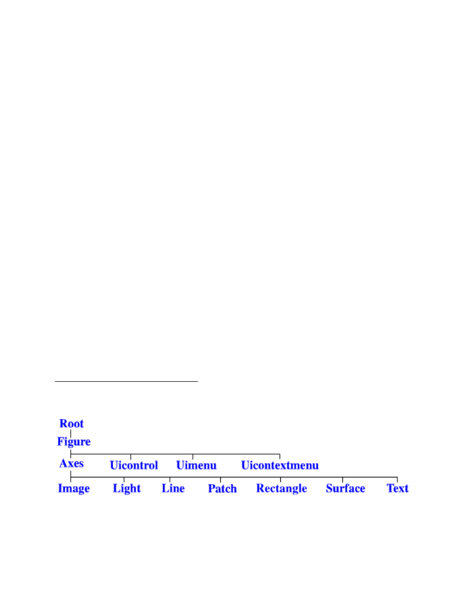
Graphical objects are classified by type. The available types lie in a strict hierarchy, as shown
in Figure
. Each figure has its own window. Inside a figure is one or more axes (ignore the other
types on this level until section
). You can make an existing figure or axes “current” by clicking
on it.
Inside the axes are drawn data-bearing objects like lines and surfaces. While there are functions
called
line
and
surface
, you will very rarely use those. Instead you use friendlier functions that
create these object types.
5.1
2-D plots
The most fundamental plotting command is
plot
. Basically, it plots points, given by vectors of x
and y coordinates, with straight lines drawn in between them.
Here is a simple example.
>> t = pi*(0:0.02:2);
>> plot(t,sin(t))
A new line object is drawn in the current axes of the current figure (these are created if necessary).
The line may appear to be a smooth, continuous curve. However, it’s really just a game of “connect
the dots,” as you can see by entering
>> plot(t,sin(t),’o-’)
Now a circle is drawn at each of the points that are being connected. Just as
t
and
sin(t)
are
really vectors, not functions, curves in MATLAB are really joined line segments.
If you now say
8
A significant difference from Maple and other packages is that if the viewpoint is rescaled to zoom in, the “dots”
are not recomputed to give a smooth curve.
Figure 1: Graphics object hierarchy.

5
GRAPHICS
32
>> plot(t,cos(t),’r’)
you will get a red curve representing cos
(
t
)
. The curve you drew earlier is erased. To add curves,
rather than replacing them, use
hold
.
>> plot(t,sin(t),’b’)
>> hold on
>> plot(t,cos(t),’r’)
You can also do multiple curves in one shot, if you use column vectors:
>> t = (0:0.01:1)’;
>> plot(t,[t t.ˆ2 t.ˆ3])
Here you get no control (well, not easily) over the colors used.
Other useful 2D plotting commands are given in Table
. See a bunch more by typing
help
graph2d
.
Table 6: 2D plotting commands
figure
Open a new figure window.
subplot
Multiple axes in one figure.
semilogx
,
semilogy
,
loglog
Logarithmic axis scaling.
axis
,
xlim
,
ylim
Axes limits.
legend
Legend for multiple curves.
Send to printer.
You may zoom in to particular portions of a plot by clicking on the magnifying glass icon in
the figure and drawing a rectangle. See
help zoom
for more details.
5.2
3-D plots
Plots of surfaces and such for functions f
(
x, y
)
also operate on the “connect the dots” principle,
but the details are more difficult. The first step is to create a grid of points in the xy-plane. These
are the points where f is evaluated to get the “dots.”
Here is a typical example:
>> x = pi*(0:0.02:1);
>> y = 2*x;
>> [X,Y] = meshgrid(x,y);
>> surf(X,Y,sin(X.ˆ2+Y))
The key step is in using
meshgrid
to make the xy grid. To see this underlying grid, try
plot(X(:),Y(:),’k.’)
.
The command
surf
makes a solid-looking surface;
mesh
makes a “wireframe” surface. In both
cases color as well as apparent height signal the values of f . Use the rotation button in the figure
window (counterclockwise arrow) to manipulate the 3D viewpoint.
The most common 3D plotting commands are shown in Table

5
GRAPHICS
33
Table 7: 3D plotting commands
surf
,
mesh
,
waterfall
Surfaces in 3D.
colorbar
Show color scaling.
plot3
Curves in space.
pcolor
Top view of a colored surface.
contour
,
contourf
Contour plot.
5.3
Annotation
A bare graph with no labels or title is rarely useful. The last step before printing or saving is
usually to label the axes and maybe give a title. For example,
>> t = 2*pi*(0:0.01:1);
>> plot(t,sin(t))
>> xlabel(’time’)
>> ylabel(’amplitude’)
>> title(’Simple Harmonic Oscillator’)
By clicking on the “A” button in the figure window, you can add text comments anywhere on
the graph. You can also use the arrow button to draw arrows on the graph. This combination is
often a better way to label curves than a legend.
5.4
Quick function plots
Sometimes you don’t want the hassle of picking out the plotting points for yourself, especially if
the function varies more in some places than in others. There is a series of commands for plotting
functional expressions directly.
>> ezplot(’exp(3*sin(x)-cos(2*x))’,[0 4])
>> ezsurf(’1/(1+xˆ2+2*yˆ2)’,[-3 3],[-3 3])
>> ezcontour(’xˆ2-yˆ2’,[-1 1],[-1 1])
5.5
Handles and properties
Every rendered object has a handle, which is basically an ID number. This handle can be used
to look at and change the object’s properties, which control just about every aspect of the object’s
appearance and behavior. (You can see a description of all property names in the Help Browser.)
Handles are returned as outputs of most plotting commands. You can get the handles of the
current figure, current axes, or current object (most recently clicked) from
gcf
,
gca
, and
gco
. The
handle of a figure is just the integer number of the figure window, and the Root object has handle
zero.
Properties are accessed by the functions
get
and
set
, or by enabling “Edit Plot” in a figure’s
Tools menu and double-clicking on the object. Here is just a taste of what you can do:

5
GRAPHICS
34
>> h = plot(t,sin(t))
>> set(h,’color’,’m’,’linewidth’,2,’marker’,’s’)
>> set(gca,’pos’,[0 0 1 1],’visible’,’off’)
Here is a way to make a “dynamic” graph or simple animation:
>> clf, axis([-2 2 -2 2]), axis equal
>> h = line(NaN,NaN,’marker’,’o’,’linesty’,’-’,’erasemode’,’none’);
>> t = 6*pi*(0:0.02:1);
>> for n = 1:length(t)
set(h,’xdata’,2*cos(t(1:n)),’ydata’,sin(t(1:n)))
pause(0.05)
end
Because of the way handle graphics works, plots in MATLAB are usually created first in a basic
form and then modified to look exactly as you want. An exception is modifying property defaults.
Every property of every graphics type has a default value used if nothing else is specified for an
object. You can change the default behavior by resetting the defaults at any level above the object’s
type. For instance, to make sure that all future Text objects in the current figure have font size 10,
say
>> set(gcf,’defaulttextfontsize’,10)
If you want this to be the default in all current and future figures, use the root object
0
rather than
gcf
.
5.6
Color
The coloring of lines and text is easy to understand. Each object has a Color property that can be
assigned an RGB (red, green, blue) vector whose entries are between zero and one. In addition
many one-letter string abbreviations are understood (see
help plot
).
Surfaces are different. To begin with, the edges and faces of a surface may have different
color schemes, accessed by EdgeColor and FaceColor properties. You specify color data at all the
points of your surface. In between the points the color is determined by shading. In flat shading,
each face or mesh line has constant color determined by one boundary point. In interpolated
shading
, the color is determined by interpolation of the boundary values. While interpolated
shading makes much smoother and prettier pictures, it can be very slow to render, particularly on
printers.
Finally, there is faceted shading which uses flat shading for the faces and black for the
edges. You select the shading of a surface by calling
shading
after the surface is created.
Furthermore, there are two models for setting color data:
Indirect
Also called indexed. The colors are not assigned directly, but instead by indexes in a
lookup table called a colormap. This is how things work by default.
Direct
Also called truecolor. You specify RGB values at each point of the data.
9
In fact it’s often faster on a printer to interpolate the data yourself and print it with flat shading. See
interp2
to
get started on this.

5
GRAPHICS
35
Truecolor is more straightforward, but it produces bigger files and is more platform-dependent.
Use it only for photorealistic images.
Here’s how indirect mapping works. Just as a surface has XData, YData, and ZData properties,
with axes limits in each dimension, it also has a CData property and “color axis” limits. The color
axis is mapped linearly to the colormap, which is a 64
×
3 list of RGB values stored in the figure.
A point’s CData value is located relative to the color axis limits in order to look up its color in
the colormap. By changing the figure’s colormap, you can change all the surface colors instantly.
Consider these examples:
>> [X,Y,Z] = peaks;
% some built-in data
>> surf(X,Y,Z), colorbar
>> caxis
% current color axis limits
ans =
-6.5466
8.0752
>> caxis([-8 8]), colorbar
% a symmetric scheme
>> shading interp
>> colormap pink
>> colormap gray
>> colormap(flipud(gray))
% reverse order
By default, the CData of a surface is equal to its ZData. But you can make it different and
thereby display more information. One use of this is for functions of a complex variable.
>> [T,R] = meshgrid(2*pi*(0:0.02:1),0:0.05:1);
>> [X,Y] = pol2cart(T,R);
>> Z = X + 1i*Y;
>> W = Z.ˆ2;
>> surf(X,Y,abs(W),angle(W)/pi)
>> axis equal, colorbar
>> colormap hsv
% ideal for this situation
5.7
Saving figures
It often happens that a figure needs to be changed long after its creation. You can save the com-
mands that created the figure as a script (section
), but this has drawbacks. If the data take a
long time to generate, rerunning the script will waste time. Also, graphical edits will be lost.
Instead, you can save figures in a native format. Just enter
>> saveas(gcf,’myfig.fig’)
to save the current figure in a file
myfig.fig
. Later you can enter
openfig myfig
to recreate
it, and continue editing.
5.8
Graphics for publication
There are three major issues that come up when you want to include some MATLAB graphics in
a document:
5
GRAPHICS
36
• file format
• size and position
• color
It helps to realize that what you see on the screen is not really what you get on paper.
To a certain extent, the file format you should use depends on your computer platform and
word processor. The big difference is between vector (representing the lines in an image) and
bitmap (a literal pixel-by-pixel snapshot) graphics. Bitmaps are great for photographs, but for
most other scientific applications they are a bad idea. These formats fix the resolution of your
image forever, but the resolution of your screen, your printer, and a journal’s printer are all very
different. These formats include GIF, JPEG, PNG, and TIFF.
Vector formats are usually a much
better choice. They include EPS and WMF.
EPS files (encapsulated postscript) are usually the right choice for documents in L
A
TEX. (They
also work in MS Word if you use a postscript printer.) For example, to save MATLAB Figure 2 as
file
myfig.eps
, use
>> saveas(2,’myfig.eps’)
A common problem with publishing MATLAB graphs has to do with size. By default, MAT-
LAB figures are rendered at 8 inches by 6 inches on paper. This is great for private use, but too
large for most journal papers. It’s easy in L
A
TEX and other word processors to rescale the image to
a more reasonable size. Most of the time, this is the wrong way to do things. The proper way is to
scale the figure before saving it.
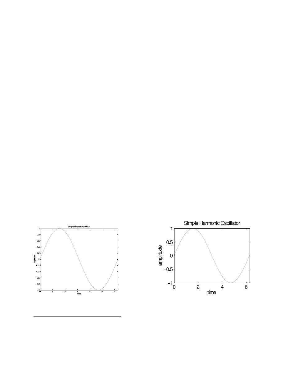
Here are two versions of an annotated graph. On the left, the figure was saved at default size
and then rescaled in L
A
TEX. On the right, the figure was rescaled first.
On the figure that is shrunk in L
A
TEX, the text has become so small that it’s hard to read. To pre-
shrink a figure, before saving you need to enter
10
JPEG is especially bad for line drawings since it is also “lossy.”

5
GRAPHICS
37
>> set(gcf,’paperpos’,[0 0 3 2.25])
where the units are in inches. (Or see the File/Page Setup menu of the figure.) Unfortunately,
sometimes the axes or other elements need to be repositioned. To make the display match the
paper output, you should enter
>> set(gcf,’unit’,’inch’,’pos’,[0 0 3 2.25])
It might be desirable to incorporate such changes into a function. Here is one that also forces a
smaller font size of 8 for all Axes and Text objects (see section
function h = journalfig(size)
pos = [0 0 size(:)’];
h = figure(’unit’,’inch’,’position’,pos,’paperpos’,pos);
set(h,’defaultaxesfontsize’,8,’defaulttextfontsize’,8)
movegui(h,’northeast’)
Most monitors are in color, but most journals do not accept color. Colored lines are automat-
ically converted to black when saved in a non-color format. The colors of surfaces are converted
to grayscale, but by default the colors on a surface range from blue to red, which in grayscale are
hard to tell apart. You might consider using
colormap(gray)
or
colormap(flipud(gray))
,
whichever gives less total black. Finally, the edges of mesh surfaces are also converted to gray,
and this usually looks bad. Make them all black by entering
>> set(findobj(gcf,’type’,’surface’),’edgecolor’,’k’)
If you do want to publish color figures, you must add an
’epsc’
argument in
saveas
.
I recommend saving each figure in graphical (EPS) format and in
fig
format (section
) with
the same name, all in a separate figure directory for your paper. That way you have the figures,
and the means to change or recreate them, all in one place.
5.9
Exercises
1. Recall the identity
e
=
lim
n
→
∞
r
n
,
r
n
=
1
+
1
n
n
.
Make a standard and a log-log plot of e
−
r
n
for n
=
5, 10, 15, . . . , 500. What does the log-log
plot say about the asymptotic behavior of e
−
r
n
?
2. Play the “chaos game.” Let P
1
, P
2
, and P
3
be the vertices of an equilateral triangle. Start
with a point anywhere inside the triangle. At random, pick one of the three vertices and
move halfway toward it. Repeat indefinitely. If you plot all the points obtained, a very clear
pattern will emerge. (Hint: This is particularly easy to do if you use complex numbers. If
z
is complex, then
plot(z)
is equivalent to
plot(real(z),imag(z))
.)
3. Make surface plots of the following functions over the given ranges.

5
GRAPHICS
38
(a)
(
x
2
+
3y
2
)
e
−
x
2
−
y
2
,
−
3
≤
x
≤
3,
−
3
≤
y
≤
3
(b)
−
3y
/(
x
2
+
y
2
+
1
)
,
|
x
| ≤
2,
|
y
| ≤
4
(c)
|
x
| + |
y
|
,
|
x
| ≤
1,
|
y
| ≤
1
4. Make contour plots of the functions in the previous exercise.
5. Make a contour plot of
f
(
x, y
) =
e
−(
4x
2
+
2y
2
)
cos
(
8x
) +
e
−
3
((
2x
+
1
/
2
)
2
+
2y
2
)
for
−
1.5
<
x
<
1.5,
−
2.5
<
y
<
2.5, showing only the contour at the level f
(
x, y
) =
0.001.
You should see a friendly message.
6. Parametric surfaces are easily done in MATLAB. Plot the surface represented by
x
=
u
(
3
+
cos
(
v
))
cos
(
2u
)
,
y
=
u
(
3
+
cos
(
v
))
sin
(
2u
)
,
z
=
u sin
(
v
) −
3u
for 0
≤
u
≤
2π, 0
≤
v
≤
2π. (Define
U
and
V
as a grid over the specified limits, use them to
define
X
,
Y
, and
Z
, and then use
surf(X,Y,Z)
.)

6
OPTIMIZING PERFORMANCE
39
6
Optimizing performance
One often hears the complaint that “MATLAB is too slow.” While it’s true that even the best
MATLAB code may not keep up with good C code, the gap is not necessarily wide. In fact, on
core linear algebra routines such as matrix multiplication and linear system solution, there is very
little difference in performance. By writing good MATLAB programs, you can often nearly recover
the speed of compiled code.
It’s good to start by profiling your code (section
) to find out where the bottlenecks are.
6.1
Use functions, not scripts
Scripts are always read and executed one line at a time (interpreted). No matter how many times
you execute the same script, MATLAB must spend time parsing your syntax. By contrast, func-
tions are effectively compiled into memory when called for the first time or modified. Subsequent
invocations skip the interpretation step.
As a rule of thumb, scripts should be called only from the command line, and they should
themselves call only functions, not other scripts.
6.2
Preallocate memory
MATLAB hides the tedious process of allocating memory for variables. This generosity can cause
you to waste a lot of runtime, though. Consider an implementation of Euler’s method for the
vector differential equation y
0
=
Ay in which we keep the value at every time step:
A = rand(100);
y = ones(100,1);
dt = 0.001;
for n = 1:(1/dt)
y(:,n+1) = y(:,n) + dt*A*y(:,n);
end
This takes about 7.3 seconds on a certain computer. Almost all of this time, though, is spent on a
noncomputational task.
When MATLAB encounters the statement
y = ones(100,1)
, it asks the operating system
for a block of memory to hold 100 numbers. On the first execution of the loop, it becomes clear
that we actually need space to hold 200 numbers, so a new block of this size is requested. On the
next iteration, this also becomes obsolete, and more memory is allocated. The little program above
requires 1001 memory allocations of increasing size, and this task occupies most of the execution
time. Also, the obsoleted space is wasted on the machine, because MATLAB generally can’t give
it back to the operating system.
Changing the second line to
y = ones(100,1001)
changes none of the mathematics but
does all the required memory allocation at once. This is called preallocation. With preallocation
the program takes about 0.4 seconds on the same computer as before.
11
In a pinch, you can write a time-consuming function alone in C and link the compiled code into MATLAB. See
section
and the online help under “External interfaces.”

6
OPTIMIZING PERFORMANCE
40
6.3
Vectorize
Vectorization refers to the removal of
for
and
while
loops in which the iterations can be run “in
parallel.” The classic example comes from a basic implementation of Gaussian elimination:
n = length(A);
for k = 1:n-1
for i = k+1:n
s = A(i,k)/A(k,k);
for j = k:n
A(i,j) = A(i,j) - s*A(k,j);
end
end
end
Look at the innermost loop on
j
. Each iteration of the loop is independent of all the others. This
parallelism is a big hint that we could do without the loop:
n = length(A);
for k = 1:n-1
for i = k+1:n
s = A(i,k)/A(k,k);
cols = k:n;
A(i,cols) = A(i,cols) - s*A(k,cols);
end
end
This version is also more faithful to the idea of a row operation, since it recognizes vector arith-
metic. Now the innermost remaining loop is also in parallel. So it too can be removed:
n = length(A);
for k = 1:n-1
rows = k+1:n;
cols = k:n;
s = A(rows,k)/A(k,k);
A(rows,cols) = A(rows,cols) - s*A(k,cols);
end
You have to flex your linear algebra muscles a bit to see that the product in the next-to-last line is
sensible and correct (in fact, it’s a vector outer product).
We reduced the original three-loop version down to one (unavoidable) loop. Why? Until about
2002, a very good answer was that the vectorized form was much faster—by a factor of hundreds—
because loops executed slowly in MATLAB. But MathWorks has been changing this. In fact, on
my Linux machine the original code now executes faster than the vectorized code does!
At this writing, MATLAB is rather picky about what loops it can optimize and on what plat-
forms it will do so. But it’s clear that code vectorization is no longer critical in every case and
may just be a question of taste in the near future. To my way of thinking, for instance, the first
vectorization we did in the Gaussian elimination code remains valuable—it’s easier to write and

6
OPTIMIZING PERFORMANCE
41
to read. The second vectorization is harder to justify, though it does lend a new perspective on the
linear algebra going on.
The details of what loops may be accelerated comparable to vectorized code are spelled out in
the “Programming and Data Types” section of the online manual. One thing not currently accel-
erated is a call to a user-defined function. Hence, for example, “function functions” (section
should try to keep calls to
feval
outside loops when possible, and this might require some vec-
torization.
There are other contexts in which vectorization remains very natural, speed considerations
aside. One of these is the evaluation of a mathematical expression such as t sin
(
t
2
)
for all elements
of a vector:
t.*sin(t.ˆ2)
is plainer and shorter than a loop. Similarly, once you understand the
cumsum
function, computing partial sums of a geometric series by
s = cumsum( (1/3).ˆ(0:100) );
is shorter more transparent than the equivalent loop, which also requires a preallocation (sec-
tion
s = ones(1,101);
for j = 1:100, s(j+1) = s(j) + 3ˆ(-j); end
The “parallel” functions, like
sum
and
diff
, in Table
can make code more readable.
The bottom line on loops in MATLAB seems to be: They should not be written casually. You
either need to look for a vectorized alternative or take care that your loop is not unnecessarily
making your code orders of magnitude slower (see section
on profiling tools). In the future
MATLAB may be more and more forgiving when it comes to loops.
6.4
Use masking
An advanced way to remove loops is by masking. Let’s say that we have a vector
x
of values at
which we want to evaluate the function
f
(
x
) =
(
1
+
cos
(
2π x
)
,
|
x
| ≤
1
2
0,
|
x
| >
1
2
.
Here is the standard loop method:
f = zeros(size(x));
for j = 1:length(x)
if abs(x(j)) <= 0.5
f(j) = 1 + cos(2*pi*x(j));
end
end
The shorter way is to use a mask.
f = zeros(size(x));
mask = (abs(x) < 0.5);
f(mask) = 1 + cos(2*pi*x(mask));

6
OPTIMIZING PERFORMANCE
42
The mask is a logical index into
x
(see page
). You could refer, if needed, to the unmasked points
by using
˜mask
.
Consider a new version of the sum-of-primes idea from page
sum( find( isprime(1:100) ) )
Here
find
converts a logical index into an absolute one. The only disadvantage of doing so in
general is that referring to the unmasked elements becomes more difficult.
6.5
Exercises
1. Rewrite
trap
or
simp
(page
) so that it does not use any loops. (Hint: Set up a vector
of all x values and evaluate
f
for it. Then set up a vector of quadrature weights and use an
inner product.)
2. Reconsider the function
chebeval
(page
) that evaluates Chebyshev polynomials at mul-
tiple points. Write the function so that it performs as efficiently as you can make it. Among
other things, you have to choose whether to use the definition or the recursion.
3. Consider again “shuffling” a vector of integers from 1 to 52, this time with a physical in-
terpretation of a shuffle. Divide the cards into two stacks, and merge the stacks together
from the bottom up. Then, each time a pair of cards is to fall off the bottom of each stack,
a random decision is made as to which falls first. This can be implemented without loops
in as little as four lines. (It can be interesting to start with a perfectly ordered deck and see
how many shuffles it takes to “randomize” it. One very crude measure of randomness is
corrcoef(1:52,v)
.)
4. Rewrite the function
entropy
on page
without any loops using
sort
,
diff
,
find
, and
(perhaps)
sum
.
5. In the function
newton
(page
), suppose that input
x0
is actually a vector of initial guesses,
and you want to run Newton’s method on each. Keep track of an error vector and use
masking to rewrite
newton
so that it still uses only one loop.
6. Rewrite
expss
from page
so that it works on a vector input and as fast as possible. (You
should consider, for example, whether making use of
persistent
variables might help.)

7
ADVANCED DATA STRUCTURES
43
7
Advanced data structures
Not long ago, MATLAB viewed every variable as a matrix or array. While this point of view is
ideal for simplicity, it is too limited for some tasks. A few additional data types are provided.
7.1
Strings
As we have seen, a string in MATLAB is enclosed in single forward quotes. In fact a string is
really just a row vector of character codes. Because of this, strings can be concatenated using
matrix concatenation.
>> str = ’Hello world’;
>> str(1:5)
ans =
Hello
>> double(str)
ans =
72
101
108
108
111
32
119
111
114
108
100
>> char(ans)
ans =
Hello world
>> [’Hello’,’ ’,’world’]
ans =
Hello world
You can convert a string such as ’3.14’ into its numerical meaning (not its character codes) by
using
eval
or
str2num
on it. Conversely, you can convert a number to string representation
using
num2str
or the much more powerful
sprintf
(see below). If you want a quote character
within a string, use two quotes, as in
’It’’s Cleve’’s fault’
.
Multiple strings can be stored as rows in an array. However, arrays have to have to be rect-
angular (have the same number of columns in each row), so strings may have to be padded with
extra blanks at the end. The function
str2mat
does this.
>> str2mat(’Goodbye’,’cruel’,’world’)
ans =
Goodbye cruel world
>> size(ans)
ans = 3 8

7
ADVANCED DATA STRUCTURES
44
There are lots of string handling functions. See
help strfun
. Here are a few:
>> upper(str)
ans =
HELLO WORLD
>> strcmp(str,’Hello world’)
ans =
1
>> findstr(’world’,str)
ans =
7
Formatted output
For the best control over conversion of numbers to strings, use
sprintf
or (for direct output)
fprintf
. These are closely based on the C function printf, with the important enhancement that
format specifiers are “recycled” through all the elements of a vector or matrix (in the usual row-
first order).
For example, here’s a script that prints out successive Taylor approximations for e
1
/
4
.
x=0.25;
n=1:8;
c=1./cumprod([1 n]);
for k=1:9,
T(k)=polyval(c(k:-1:1),x);
end
fprintf(’\n
T_n(x)
|T_n(x)-exp(x)|\n’);
fprintf(’----------------------------------\n’);
fprintf(’%15.12f
%8.3e\n’, [T;abs(T-exp(x))] )
T_n(x)
|T_n(x)-exp(x)|
----------------------------------
1.000000000000
2.840e-01
1.250000000000
3.403e-02
1.281250000000
2.775e-03
1.283854166667
1.713e-04
1.284016927083
8.490e-06
1.284025065104
3.516e-07
1.284025404188
1.250e-08
1.284025416299
3.892e-10
1.284025416677
1.078e-11

7
ADVANCED DATA STRUCTURES
45
7.2
Cell arrays
Collecting objects (such as strings) that have different sizes is a recurring problem. Suppose you
want to tabulate the Chebyshev polynomials: 1, x, 2x
2
−
1, 4x
3
−
3x, etc. In MATLAB one ex-
presses a polynomial as a vector (highest degree first) of its coefficients. The number of coeffi-
cients needed grows with the degree of the polynomial. Although you can put all the Chebyshev
coefficients into a triangular array, this is an inconvenient complication.
Cell arrays
are used to gather (potentially) dissimilar objects into one variable. They are in-
dexed like regular numeric arrays, but their elements can be absolutely anything. A cell array is
created or referenced using curly braces
{}
rather than parentheses.
>> str =
{
’Goodbye’, ’cruel’, ’world’
}
str =
’Goodbye’
’cruel’
’world’
>> str
{
2
}
ans =
cruel
>> T = cell(1,9);
>> T(1:2) =
{
[1], [1 0]
}
;
>> for n = 2:8,
T
{
n+1
}
= [2*T
{
n
}
0] - [0 0 T
{
n-1
}
];
end
>> T
T =
Columns 1 through 5
[1]
[1x2 double]
[1x3 double]
[1x4 double]
[1x5 double]
Columns 6 through 9
[1x6 double]
[1x7 double]
[1x8 double]
[1x9 double]
>> T
{
4
}
ans =
4
0
-3
0
Cell arrays can have any size and dimension, and their elements do not need to be of the same
size or type. Cell arrays may even be nested. Because of their generality, cell arrays are mostly just
containers; they do not support any sort of arithmetic.
One special cell syntax is quite useful. The idiom
C
{
:
}
for cell array
C
is interpreted as a
comma-separated list of the elements of
C
, just as if they had been typed. For example,
>> str2mat(str
{
:
}
)
% same as str2mat(’Goodbye’,’cruel’,’world’)

7
ADVANCED DATA STRUCTURES
46
ans =
Goodbye
cruel
world
The special cell array
varargin
is used to pass optional arguments into functions. For exam-
ple, consider these modifications to the bisection algorithm on page
function x = bisect(f,a,b,varargin)
fa = feval(f,a,varargin
{
:
}
);
fb = feval(f,b,varargin
{
:
}
);
...
If arguments beyond the first three are passed in to
bisect
, they are passed along to
f
. Naturally,
in other contexts you are free to look at the elements of
varargin
and interpret them yourself.
There is also a
varargout
for optional outputs.
7.3
Structures
Structures are much like cell arrays, but they are indexed by names rather than by numbers.
Say you are keeping track of the grades of students in a class. You might start by creating a
student
struct
(structure) as follows:
>> student.name = ’Clinton, Bill’;
>> student.SSN = 123456789;
>> student.homework = [10 10 7 9 10];
>> student.exam = [98 94];
>> student
student =
name: ’Clinton, Bill’
SSN: 123456789
homework: [10 10 7 9 10]
exam: [98 94]
The name of the structure is
student
. Data is stored in the structure according to named fields,
which are accessed using the dot notation above. The field values can be anything.
Probably you have more students.
>> student(2).name = ’Bush, G. W.’;
>> student(2).SSN = 987654321;

7
ADVANCED DATA STRUCTURES
47
>> student(2).homework = [4 6 7 3 0];
>> student(2).exam = [53 66];
>> student
student =
1x2 struct array with fields:
name
SSN
homework
exam
Now you have an array of structures. As always, this array can be any size and dimension. How-
ever, all elements of the array must have the same fields.
Struct arrays make it easy to extract data into cells:
>> [roster
{
1:2
}
] = deal(student.name)
roster =
’Clinton, Bill’
’Bush, G. W.’
In fact,
deal
is a very handy function for converting between cells and structs. See online help for
many examples.

8
GRAPHICAL USER INTERFACES
48
8
Graphical user interfaces
Most of us rely on graphical user interfaces (GUI) at least part of the time. They are especially
useful to nonexpert users. Adding a GUI to a software package is not too hard in MATLAB, once
you have acquired the skill. Although GUI programming is not inherently stimulating, a well-
designed GUI is appreciated by others and makes your work more significant.
By the way, the principles of GUI programming are pretty universal, so learning them in MAT-
LAB is good training for writing GUIs in other environments, such as Java.
8.1
GUI programming style
Scientific programs are usually written in a procedural style: You give a list of instructions, tell the
computer to start execution at the beginning, and wait for the computer to finish the instructions.
This model doesn’t hold up for GUI programming. A GUI creates buttons, menus, and other
objects (collectively called widgets) and then waits for the user to do something. When an action
is taken, the GUI may be expected to respond in some way, then resume waiting. This is event-
driven
programming, and it requires a different style that at first may seem cumbersome.
Each widget has a state and perhaps a callback function. The state of a widget includes its
label, position, and current value. The callback is a function that is executed in the base workspace
each time the widget is selected or has its value changed. In MATLAB there can also be callback
functions for certain other events, such as pressing keys, moving the mouse in the figure window,
or resizing the figure window.
Most GUIs, for example, have a “quit” button that, when pressed, might ask for confirmation
and then destroy the window that the GUI is in. Here is a sketch of this behavior in MATLAB:
uicontrol(’style’,’pushbutton’,’label’,’Quit’,’callback’,@GUIQuit)
% later on in the file...
function GUIQuit
a = questdlg(’Really quit?’,’Confirm quit’,’Yes’,’No’,’No’);
if strcmp(a,’Yes’)
delete(gcbf)
end
Remember that
@GUIQuit
is a function handle in MATLAB. The built-in
questdlg
opens a win-
dow with a question and gets an answer from the user. The function
gbcf
stands for “get callback
figure,” i.e., the handle of the figure that the button is in.
In addition to creating the widgets and filling in the appropriate callback actions, GUI pro-
grams usually need a mechanism for holding “global” data. For instance, some widgets may hold
settings that affect the actions of the callbacks, so their handles should be public knowledge.
8.2
Using guide for layout
Laying out the physical appearance of the GUI is the first and easiest step. Before using the com-
puter, you should invest some time with paper or chalkboard deciding what elements should be

8
GRAPHICAL USER INTERFACES
49
in your GUI and what they will do. GUIs tend to be more globally coupled than other types of
programs, so making changes later on can take a fair amount of work.
Once you are ready, type
guide
to get a GUI for making GUIs. Using
guide
you can add
widgets and axes to a figure and make it all look the way you want. Double-click on a widget
to edit its properties. Always important are the String, which is usually the label of the widget,
and the Tag, which is an internal designation. It is usually wise to give the tags some consistency.
For instance, a slider that controls a quantity β would be
BetaSlider
, the quit button would be
QuitButton
, etc. Leave the Callback property set to “automatic,” unless you are sure you can
delete it.
After the GUI looks OK and all widgets have the correct properties, ask
guide
to “activate”
the figure. This will create a
fig
file (section
) that records the layout of the GUI, and an M-file
(section
) with the skeleton of the function that will implement the GUI.
8.3
Creating callbacks
The skeleton created by
guide
has a short main section followed by empty “stubs” for callback
functions. You are expected to edit the skeleton in order to make the callbacks work as intended.
The main section of the GUI M-file takes one of two possible actions:
• If the GUI M-file is called with no input arguments (as when it is typed at the command line),
then the GUI is launched, either by loading the
fig
file or by bringing forward a preexisting
GUI window.
• Otherwise, the input arguments represent a callback invocation, and the main section passes
control to the correct callback subfunction. This is called a switchyard programming model.
The standard callback assigned to a GUI widget involves the Tag property of the widget. For
example, the callback for a button with the Tag
QuitButton
in a GUI figure named
mygui
will
have callback
mygui(’QuitButton_Callback’,gcbo,[],guidata(gcbo))
The argument
gcbo
(“get callback object”) gives the handle of the widget whose callback is ex-
ecuting. The second argument is always empty in MATLAB 6.0 but in the future may contain
information about the event that caused the callback invocation.
The function
guidata
provides the standard mechanism for storing global data in a GUI.
There are two ways to call it:
data = guidata(h);
guidata(h,data)
The first call retrieves
data
and the second stores it.In both cases,
h
is the handle of the GUI figure
or any object in it. By default when using
guide
,
data
is a structure (section
) whose fields are
the Tag names of GUI widgets and whose values are the handles of those widgets. Thus you at
least have access to all the tagged widgets in the GUI. But
data
is an ordinary structure, so you
can add fields holding whatever objects you like. Just remember to store
data
again after making
any changes to it.
12
Often a cell array (section
) of strings here is interpreted as one string per text line.

8
GRAPHICAL USER INTERFACES
50
8.4
An example
Here is a function that creates a simple GUI, for a “Monte Carlo” estimate of π. It has a slider called
NumberSlider
that sets the number of samples, a
ComputeButton
that causes the estimate to
be computed, and two other buttons that create different plots of the data. Don’t be too concerned
with the gritty details of each callback—just try to see the overall structure, and how the global
data are passed around.
function varargout = montecarlo(varargin)
if nargin == 0
% LAUNCH GUI
fig = openfig(mfilename,’reuse’);
set(fig,’Color’,get(0,’defaultUicontrolBackgroundColor’));
handles = guihandles(fig);
guidata(fig, handles);
NumberSlider_Callback(handles.NumberSlider,[],handles);
if nargout > 0
varargout1 = fig;
end
elseif ischar(varargin1) % INVOKE NAMED SUBFUNCTION OR CALLBACK
try
[varargout1:nargout] = feval(varargin:); % FEVAL switchyard
catch
disp(lasterr);
end
end
function varargout = NumberSlider_Callback(h, eventdata, handles, varargin)
set(handles.PointsButton,’enable’,’off’)
set(handles.ConvergenceButton,’enable’,’off’)
function varargout = ComputeButton_Callback(h, eventdata, handles, varargin)
setptr(handles.MonteCarloFigure,’watch’)
rand(’state’,sum(100*clock))
% alter seed state
N = get(handles.NumberSlider,’value’);
N = round(N);
x = 2*rand(N,2) - 1;
absx2 = sum( x.ˆ2, 2);
estimate = cumsum( absx2<1 );
estimate = 4 * estimate ./ (1:N)’;
setptr(handles.MonteCarloFigure,’arrow’)
handles.x = x;
handles.estimate = estimate;
guidata(h,handles);
set(handles.PointsButton,’enable’,’on’)
set(handles.ConvergenceButton,’enable’,’on’)

8
GRAPHICAL USER INTERFACES
51
function varargout = PointsButton_Callback(h, eventdata, handles, varargin)
x = handles.x;
figure
t = pi*(0:0.01:2);
plot(cos(t),sin(t),’r’,’linewidth’,2)
hold on
plot(x(:,1),x(:,2),’k.’,’markersize’,1)
axis equal, axis square
axis([-1.05 1.05 -1.05 1.05])
function varargout = ConvergenceButton_Callback(h, eventdata, handles, varargin)
est = handles.estimate;
figure
loglog( 1:length(est), abs(pi-est) )
function varargout = QuitButton_Callback(h, eventdata, handles, varargin)
delete(gcbf)

9
OBJECT-ORIENTED PROGRAMMING
52
9
Object-oriented programming
Object-oriented programming
(OOP) is a paradigm meant to aid in the development and main-
tenance of large programming projects. It some ways it differs significantly from the functional
programming that dominates the history of computing (and most current scientific computing).
Although not designed with an interactive system like MATLAB in mind, OOP brings benefits to
it as well, chiefly in the design of self-contained packages.
The major concepts of OOP are
Encapsulation
Different kinds of data are collected into one named object. An object’s contents
cannot be altered directly. Instead one must use procedures called methods for operating on
the data.
Inheritance
Objects can be defined in a hierarchy in which “child” objects can inherit data formats
and methods from its “parent.”
Overloading
Operators and functions that are already defined in other contexts can be extended
to work with new object types.
Each of these is supported by MATLAB, although not to the extent of a language such as Java
or C++.
9.1
OOP in MATLAB
You define a class of objects that spells out the data held by an object and the methods defined
for it. The methods are regular functions in a special directory whose name must start with the
at-sign @. If that directory is on the MATLAB path, you can then create instances of the class to
hold data.
Every class must include a special method called the constructor, which has the same name as
the class directory (without @). The constructor lays out in a structure (section
) the template
of data needed for this object and initializes the data as it sees fit. Once the structure is ready,
the constructor calls
class
to create an object instance. (Users and other functions may also use
class
to inquire about an object’s type.) Once an instance is constructed, the methods in the class
directory are the only functions that can operate on it.
The constructor may choose to signify that the current class is a child of another existing class.
In that case, the child object inherits all of the data fields and methods of the parent class. Inher-
itance is often used to implement the “is a” relationship; object types that are more specific than
some other type may logically inherit from that type. For instance, a circle is a special kind of
ellipse. Anything you might want to know about or do to an ellipse could also be asked of a circle.
However, a circle is more specific and might support additional operations not known to ellipses
(like a “radius” method).
Methods in a class directory that have the same name as other MATLAB functions will over-
load
those functions when called on an instance of the object. For example, a
circle
class might
13
MathWorks has made integration with Java a priority in recent years, however, so in a sense this is changing.

9
OBJECT-ORIENTED PROGRAMMING
53
have a method called
plot
that knows how to plot a circle. You are even allowed to overload
built-in operators such as
+,*,/,.*
, etc. Each of these actually has a full function name (
plus
or
uplus
,
mtimes
,
mrdivide
, and
times
for the examples above) that can be overloaded. You
can also overload transposition, array concatenation, and array subscript referencing, so that (for
instance)
p(i)
might return the ith vertex of polygon
p
. (For a complete list of overloadable
operators, type
help *
.) Another important overloadable function is
display
, which controls
what MATLAB types out when an object is the result of an expression that does not end with a
semicolon.
9.2
An OOP example
Let’s look at an object class for polygons. Here is the constructor, in
@polygon/polygon.m
.
function p = polygon(x,y)
superiorto(’double’);
if nargin==0
% Template call.
p.x = [];
p.y = [];
else
if length(x)˜=length(y) | length(x)<3
error(’Invalid vertex data.’)
end
p.x = x;
p.y = y;
end
p = class(p,’polygon’);
Note that the data defining
p
are created just like a structure (section
). The call to
class
must
be done after all the fields of
p
have been created. The
nargin==0
case is important: If a MAT-file
containing a polygon object is loaded into the workspace, MATLAB will call the constructor with
no arguments in order to see what fields a polygon ought to have. Finally, the call to
superiorto
is useful for overloading. It says that function calls that have both polygons and doubles (i.e.
numbers, or arrays of numbers) should look first for polygon methods before applying functions
for doubles. The default behavior is to give priority based on ordering of the function arguments,
so
p+2
and
2+p
would be interpreted differently.
Next we write a function
@polygon/display.m
:
function display(p)
n = length(p.x);
if n < 10
% Show all vertices
fprintf(’\n
Polygon with vertices\n\n’)
fprintf(’
(%8.3g,%8.3g)\n’,[p.x’; p.y’])

9
OBJECT-ORIENTED PROGRAMMING
54
else
% Summary only
fprintf(’\n
Polygon with %i vertices\n’,n)
end
fprintf(’\n’)
Now, if you enter
p=polygon([-0.5,1,-1],[2,0,2])
, you will see
Polygon with vertices
(
-0.5,
2)
(
1,
0)
(
-1,
2)
However, trying to reference
p.x
from the command line will give an error. Only
polygon
meth-
ods are permitted to access the object data directly.
Next we extend
plot
to understand polygons.
function h = plot(p,varargin)
if nargin==1
% Default plot style
varargin =
{
’b.-’,’markersize’,10,’markeredgecolor’,’k’
}
;
end
xx = p.x([1:end 1]);
yy = p.y([1:end 1]);
hh = plot(xx,yy,varargin
{
:
}
);
axis equal
if nargout > 0,
h = hh;
end
You can then use
plot(p)
to see a plot of the polygon.
It might be nice to be able to rotate a polygon about a specified center.
function q = rotate(p,center,theta)
xy(:,1) = p.x - center(1);
xy(:,2) = p.y - center(2);
A = [cos(theta) -sin(theta); sin(theta) cos(theta)];
xy = (A*xy’)’;
% or xy*A’;
q = polygon( xy(:,1)+center(1), xy(:,2)+center(2) );
Translation can be expressed by adding a 2-element vector.
function q = plus(p,v)
if isa(v,’polygon’)
tmp = v;
v = p;
p = tmp;
end
q = polygon( p.x+v(1), p.y+v(2) );

9
OBJECT-ORIENTED PROGRAMMING
55
Notice how the order of arguments was checked. In practice you would probably want to do more
error checking.
Another useful function is the ability to extract the numerical values of the vertices. A conve-
nient syntax is to define a method
double
, which in other contexts already means “conversion to
numerical values.”
function xy = double(p)
xy = [p.x p.y];
Much more could be added to the
polygon
class, but let’s consider creating a child class
square
. A square is a polygon, so inheritance is appropriate. However, a square might be spec-
ified by its center, orientation, and side length. The constructor
@square/square.m
could read
as follows.
function s = square(varargin)
superiorto(’double’);
if nargin==0
p = polygon;
s.center = [];
elseif nargin==2
% x, y given
[x,y] = deal( varargin: );
p = polygon(x,y);
s.center = [ mean(x) mean(y)];
else
% center, angle, sidelen given
[cen,ang,len] = deal( varargin: );
s.center = cen;
x = (0.5*len)*[-1 -1 1 1];
y = (0.5*len)*[1 -1 -1 1];
p = rotate(polygon(x,y),[0 0],ang) + cen;
end
s = class(s,’square’,p);
The last line defines
square
to be a child of class
polygon
. The object
s
will have a field named
“polygon” in which the parent instance
p
is stored and can be accessed. Every method defined for
polygons can be applied to
s
, unless it is overloaded for squares. A
square
object can also store
other kinds of data, as with the “center” field here.
Thus, if you create a
square
without a semicolon, you will get the usual
polygon
output.
This is fine, but it might be nice to signal that this is in fact a square. So we write a method
@square/display.m
:
function display(s)
xy = double(s.polygon);

9
OBJECT-ORIENTED PROGRAMMING
56
fprintf(’\n
Square with corners\n\n’)
fprintf(’
(%8.3g,%8.3g)\n’,xy’)
fprintf(’\n’)
This will overload the
@polygon/display
method when a square is involved. We can also
create a method for a
square
that has no
polygon
counterpart:
function c = center(s)
c = s.center;
9.3
Exercises
1. Use the functions you already have for polygon perimeter and area (page
) to add these
capabilities to the
polygon
class.
2. Add the ability to scale a
polygon
through the syntax of scalar multiplication. For instance,
2*p
should double all the vertices in
p
. You might then figure out how to make
-p
be
interpreted as
(-1)*p
.
3. Add the ability to extract or change a single vertex (or, if you’re ambitious, multiple vertices)
of a polygon. See the help for
subsref
and
subsasgn
.
4. Create a class
ivp
for initial-value problems for ordinary differential equations. It should
store at least the ODE (probably using a function handle) and an initial condition. Consider
how to do this so that a method
solve
could invoke a built-in ODE solver such as
ode45
to solve the IVP numerically. This too could be stored in the object so that future calls could
evaluate or plot the solution (see help for
deval
).

10
LINKING TO FORTRAN OR C
57
10
Linking to Fortran or C
[This section is really just a sketch right now.–TAD]
There are three ways that MATLAB can interface to code written in Fortran or C:
• Calling Fortran or C routines from MATLAB (MEX interface).
• Calling MATLAB functions from C or Fortran (Engine services).
• Converting MATLAB code to standalone C (MATLAB–C Compiler).
The first option is useful when you want to speed up the execution of a slow MATLAB function, or
when you want to take advantage of previously written code, such as that available on
netlib
.
The second option can use MATLAB as a computational “backend” for a “frontend” interface
written in another language, or to use MATLAB graphics from another program. The final option
can create fast, independent programs that were originally developed in the convenient MATLAB
environment.
Here we discuss only MEX files. The discussion centers on Fortran, but C files are very similar
(and perhaps a bit easier).
10.1
How MEX files work
MEX files work like alternatives to M-files. The name of a MEX file on the path can be invoked
in MATLAB just like any other function. A MEX file is created by compiling code consisting of
two main parts: a computational part, which is usually ordinary code, and a gateway section that
knows how to exchange data with MATLAB.
There are some major differences between MEX files and M-files:
• Since they come from compiled and linked Fortran or C, MEX files are platform-dependent
and need to be constructed in a separate step.
• Memory management is much more the responsibility of the programmer than in M-files.
They do not get their own workspace, but can operate in the caller’s workspace.
• MEX files do not carry documentation that can be found by
help
. Instead, you put the
documentation into an otherwise empty M-file of the same name.
Every variable in MATLAB has a value that is called an
mxArray
in a MEX file. An
mxArray
has information about the data type of the variable (double, string, cell array, etc.), its size, and
pointers to its data. The data of a double-class array are stored in separate arrays of real and
imaginary parts, in the Fortran row-varying-first order.
The MEX gateway operates on an
mxArray
through routines whose names start with
mx
.
There are also functions starting with
mex
for working with the MATLAB process (e.g., to evaluate
commands). These external functions are linked automatically when you compile the code using
the
mex
script provided with MATLAB.
14
It’s worth mentioning here as well that MATLAB can instantiate and act on objects from any externally defined
Java class directly. See the online help for
java
.

10
LINKING TO FORTRAN OR C
58
10.2
Examples and outline
Some MEX examples are in the directory
extern/examples/refbook
found in the main MAT-
LAB installation directory. These are discussed in the online “External Interfaces” manual. To try
them, follow the instructions in the manual.
The gateway always begins with the line
subroutine mexfunction(nlhs,plhs,nrhs,prhs)
This is how the gateway will access the input (RHS) and output (LHS) arguments to the MEX
function call. The basic outline is
1. Get basic info (sizes, classes, etc.) about input arguments and check their validity.
2. Create an
mxArray
for each of the
nlhs
outputs.
3. Call the computational section, using indirection to make the MATLAB data look like regular
Fortran arrays.
4. Store the computational results in the output arguments, free any temporary variables, and
exit.
Document Outline
- Introduction
- Arrays and matrices
- Scripts and functions
- More on functions
- Graphics
- Optimizing performance
- Advanced data structures
- Graphical user interfaces
- Object-oriented programming
- Linking to Fortran or C
Wyszukiwarka
Podobne podstrony:
Dr Sulo Crash Course in NLP
04 Survival Russian a Course in Conversational Russian
A course in descriptive grammar, presentation 1
9 hot and young crash course
Crash Course Present Simple
A Complete Course In Astrology (Horoscope Interpretation)
Ash R B A course in commutativ Nieznany
04 Survival Russian a Course in Conversational Russian
A Course in Miracles Frequently Asked Questions Doug Thompson (Share Me) (ebook)
Rubenstein A Course in Game Theory SOLUTIONS
Letter of requesting course in England(1)
Crash Course HAVE
A translation course in building vocabulary
A short course in Scrying by Benjamin Rowe
Crash Course Past Simple
więcej podobnych podstron