A Performance Prediction Model for the CUDA GPGPU Platform

Kishore Kothapalli

Rishabh Mukherjee

Suhail Rehman

Suryakant Patidar

P. J. Narayanan

Kannan Srinathan

International Institute of Information Technology, Hyderabad

Gachibowli, Hyderabad, India – 500 032.

Email:

{

kkishore@,rishabh m@research., rehman@research.

}

iiit.ac.in

{

skp@research., pjn@, srinathan@

}

iiit.ac.in

Abstract

The significant growth in computational power of mod-
ern Graphics Processing Units(GPUs) coupled with the
advent of general purpose programming environments
like NVIDA’s CUDA, has seen GPUs emerging as a
very popular parallel computing platform. However, de-
spite their popularity, there is no performance model of
any GPGPU programming environment. The absence
of such a model makes it difficult to definitively as-
sess the suitability of the GPU for solving a particular
problem and is a significant impediment to the main-
stream adoption of GPUs as a massively parallel (su-
per)computing platform.

In this paper we present a performance prediction

model for the CUDA GPGPU platform. This model
encompasses the various facets of the GPU architec-
ture like scheduling, memory hierarchy and pipelin-
ing among others.

We also perform experiments

that demonstrate the effects of various memory access
strategies. The proposed model can be used to analyze
pseudo code for a CUDA kernel to obtain a performance
estimate, in a way that is similar to performing asymp-
totic analysis. We illustrate the usage of our model and
its accuracy, with three case studies: Matrix Multiplica-
tion, List Ranking, and histogram generation.

1

Introduction

Over the past decade, the processing power of
the Graphics Processing Units (GPUs) has increased
tremendously. The latest GPU from Nvidia, GeForce
GTX280, has a raw computing power of close to one
TFLOPS at a cost of about $400. Given this enormous
computational power, researchers have started looking
at ways to utilize this efficiently for non-graphics based
applications also.

This is termed as GPGPU (Gen-

eral Purpose Graphics Processing Units). To this end,

Nvidia now supports a C like programming language
called CUDA [4] (Compute Unified Device Architec-
ture) that allows a programmer to explicitly request that
certain portions of the code be run on the GPU

1

.

The advent of CUDA has led to several high-speed

implementations on the GPU. A few prominent ones are
given below. Image processing and filtering algorithms
are studied in [13, 26, 17]. Graph algorithms such as
BFS, Shortest paths, graph cuts, etc. are reported on the
GPU [25, 11] for large graphs. Data parallel primitives
such as parallel-prefix scan[23, 18], reduction, and sort-
ing [23] have also been studied. GPUs have also been
used to implement numerical algorithms including the
FFT [9].

Speed-up of the order of 200 over conventional CPU

implementations are reported for certain problems such
as the

n-body simulation[17, Chapter 31]. At the other

extreme, there are problems where the best reported
speedup is just about 3 [15]. While the speed-up re-
ported does depend on the hardware available at the
time it is reported, it is in general not possible to ex-
plain the origins of the speed-ups or the varying perfor-
mance across different problems. Also the relationship
between the different facets of these implementations is
not clearly understood and as such it is hard to adopt a
structured approach to optimize these implementations.
These problems are complicated by the fact that leading
manufacturers of GPUs do not divulge architectural de-
tails of their product, apart from a high level technical
specification point of view.

Thus there is a significant need to understand the

computational abilities of modern-day GPUs so as to
use them efficiently. When one considers multiproces-
sor architectures, there are several issues that one has to
contend with apart from computations, viz. the mem-
ory hierarchy, the interprocess communication, syn-

1

Another popular vendor of GPUs, AMD similarly supports a

combination of a low-level interface, the Compute Abstraction Layer
(CAL) and extensions to Brook.

1

chronization, and the like. When working at a purely al-
gorithmic level, and ignoring the effects of memory hi-
erarchy, cost of synchronization, etc., the PRAM model
[6] has been a highly successful model and can give
tight asymptotic bounds on the runtime and the total
work done. But, the abstraction of the PRAM model
does not help one to choose a right algorithm for a given
architecture, for example the GPU. Hence, it is of inter-
est to see how much of architectural details should be
modeled carefully so that one can work at a level of ab-
straction that can be used to analyze algorithms and at
the same time make reasonably accurate claims.

The benefits of such a model are manifold, some of

which are given below. Firstly, it helps augment the
PRAM model to understand the limits of parallelizabil-
ity of algorithms on the GPUs. A second benefit is to
provide an informative profile of a GPU program so as
to be able to identify bottlenecks. As in the case of se-
quential architectures, we feel that a good simulator is
the need of the hour when one wishes to evaluate the
effect of certain design choices for future versions of
GPUs. Our model can help efforts in this direction.

In this paper, we propose a model for the same. Our

model coupled with relevant case-studies shall formal-
ize several aspects of GPU programming that serves to
bridge the gap between the algorithmic developments
and the application engineering. Using our model, one
can make educated claims about a program in execution
on the GPU. Note, however, that our aim is not to pro-
vide any guidelines on how to program using GPU for
good performance. This is best served by existing man-
uals such as [4]. The focus of our work is to explain the
behavior of the GPU and additionally understand the
nature of problems that scale well on the GPU.

1.1

Related Work

The parallel algorithms community has developed sev-
eral models to design and analyze parallel algorithms
such as the network model [14], the PRAM model [6],
the Log-P model [5], the QRQW model [7, 8], among
others. These models help the algorithm designer to ex-
ploit the parallelism in the problem. However, as these
are mostly architecture independent they fail to help the
algorithm designer leverage any specific advantages of-
fered by the architecture or work around the ill-effects
of any architectural limitations on the performance of
the algorithm.

As far as modeling for performance on multiproces-

sor architectures is concerned, there is very little re-
ported work. In [21], the authors discuss the parame-
ter space and present ways to prune the size of such a
space and get a highly optimized code. The result is a
gain of about 17% for a particular medical imaging ap-

plication [21]. However, our work does not target code
or runtime optimizations. An extension of this work ap-
pears in [22] where the authors consider the multi-GPU
design space optimization. However, they need a model
to predict the baseline implementation on a single GPU.
Our work can exactly fill that need. So we place our
work as complementary to that of [22]. A model sim-
ilar to ours appears in [16] where also the authors rely
on separating memory and compute requirements. But
their model is applicable only for a class of programs
called ”Iterative Stencil Loops”.

1.2

Our Results

In this paper, we propose a fairly complete performance
model for the Nvidia GPU. Our model tries to abstract
the GPU computational model by considering impor-
tant features of the present generation Nvidia GPU GTX
280. We use a combination of the BSP model of Valiant
[24], the PRAM model of Fortune and Wyllie [6], and
the extension to PRAM model proposed by Gibbons et
al. called the QRQW model [8]. We note that none
of the models individually can explain the behavior of a
GPU. We also note that slight modifications are required
to these models to model GPU computations accurately.

The proposed model outlines the relationship be-

tween the various components of the GPU architecture
like the number of cores, effects of memory latency,
memory access conflicts, cost of computing, schedul-
ing, pipelining, etc. This model can be used to analyze
pseudo-code for a CUDA kernel and finally predict the
performance, almost analogous to the way asymptotic
analysis is carried out in the case of sequential comput-
ing.

We devise experiments that showcase the effects of

memory access related issues like coalescing and bank
conflicts and the corresponding latency penalties in-
curred. We further demonstrate the use of our model on
three real-world parallel algorithms - matrix multiplica-
tion, list ranking, and histogram generation. These case
studies have been chosen so that one of them is compute
intensive, one is (global) memory intensive, and one is
shared memory based. Thus, these three case studies
cover the scope of the proposed model.

1.3

Organization of the Paper

The rest of the paper is organized as follows. In Section
2, we provide a basic introduction to the GPU computa-
tional model. In Section 3 we describe the proposed per-
formance model. Section 4 corroborates the proposed
model using targeted experiments. This is followed by
three case studies in Section 5. The paper ends with
some concluding remarks after mentioning a few limi-
tations of our model.

2

2

GPU Architecture and CUDA

Nvidia’s unified architecture (see also Figure 1(a)) for
its current line of GPUs supports both graphics and
general computing.

In general purpose computing,

the GPU is viewed as a massively multi-threaded ar-
chitecture containing hundreds of processing elements
(cores). Each core comes with a 4 stage pipeline. 8
Cores, also known as symmetric processors are grouped
in a SIMD fashion into a Symmetric Multiprocessor
(SM), so that each core in an SM executes the same
instruction. The GTX280 has 30 of these SMs, which
makes for a total of 240 processing cores. Each core can
store a number of thread contexts. Data fetch latencies
are tolerated by switching threads. Nvidia implements
a zero-overhead scheduling system by quick switching
of thread contexts in the hardware.

The CUDA API, Figure 1(b), allows a user to create

large number of threads to execute code on the GPU.
Threads are also grouped into blocks and blocks make
up a grid. Blocks are serially assigned for execution on
each SM. The blocks themselves are divided into SIMD
groups called warps, each containing 32 threads. An
SM executes one warp at a time. CUDA has a zero over-
head scheduling which enables warps that are stalled on
a memory fetch to be swapped for another warp. For
this purpose, Nvidia recommends at least 1024 threads
be assigned to an SM to keep an SM fully ’occupied’.

The GPU also has various memory types at each

level. A set of 32-bit registers is evenly divided among
the threads in each SM. 16 Kilobyte of shared mem-
ory per SM acts as a user-managed cache and is avail-
able for all the threads in a Block. The GTX 280 also
comes with 1 GB of off-chip global memory which can
be accessed by all the threads in the grid, but may in-
cur hundreds of cycles of latency for each fetch/store.
Global memory can also be accessed through two read-
only caches known as the constant memory and texture
memory for efficient access for each thread of a warp.

Computations that are to be performed on the GPU

are specified in the code as explicit Kernels. Prior to
launching the kernel, all the data required for the com-
putation must be transferred from the Host (CPU) mem-
ory to the GPU (Global) memory. A Kernel invocation
will hand over the control to the GPU, and the speci-
fied GPU code will be executed on this data. Barrier
Synchronization for all the threads in a block can be de-
fined by the user in the kernel code. Apart from this,
all the threads launched in a grid are independent and
their execution or ordering cannot be controlled by the
user. Global synchronization of all threads can only be
performed across separate kernel launches. For more
details, we refer the interested reader to [4, 18].

3

Our Performance Model for the
GPU

The model we present for the GPU is a combination of
known models of parallel computation with small ex-
tensions. Given the complex architecture of the GPU,
it turns out that none of these models suffice individu-
ally and a combination of them with a few extensions is
required. The models we use are:

• The BSP model of Valiant [24],

• The PRAM model of Fortune and Wylie [6], and

• The QRQW model of Gibbons, Matias, and Ra-

machandran [7, 8]

A brief summary of these models is given in Ap-

pendix A. In the following we describe our modeling
of the GPU using the above three models.

3.1

Synchronization Model

As discussed in Section 2, CUDA programs are written
in units called kernels. Threads start synchronously at
the beginning of each kernel and are synchronized at the
end of each kernel. Thus, the basic unit of synchroniza-
tion is the kernel. This fits the BSP model of parallel
computing quite closely, with an implicit call to syn-
chronize at the end of each kernel. Notice however that
while in the BSP model, synchronization is at regular
intervals of

L time units, our model does away with this

requirement. Given the lack of any routing infrastruc-
ture in the GPU, we rely on the BSP model only as far
as the notion of super-steps [24] is concerned.

A further facet of the GPU is that threads in a block

can all be synchronized explicitly within a kernel by a
call to the primitive

syncthreads()

. This puts

a barrier for threads in a block and it is guaranteed that
executing this call and thereby synchronizing threads in
a block takes 4 cycles, plus additional wait time depend-
ing on the circumstances. But this being an explicit and
optional call, threads need not be synchronized every 4
cycles.

It thus implies that the time taken by a GPU program

can be expressed as the sum of the times taken by the
super-steps, or kernels. For the sake of simplicity, we
ignore the effect of intra-kernel synchronization steps
such as

syncthreads() on the overall runtime. At the

end, we discuss a way to extend our model to handle
also intra-kernel synchronization.

3.2

GPU a. la. (QRQW) PRAM

The other parts of the GPU model are not as straight-
forward. We will propose a model for the GPU that

3

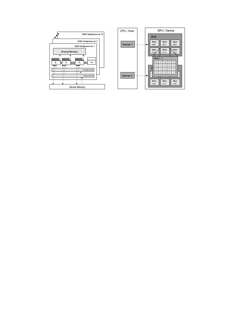
(a) CUDA GPU Memory Hierarchy

(b) Execution Model

Figure 1: The CUDA Computation Model.

accounts for its memory hierarchy along with computa-
tion.

The PRAM model (see also Appendix A is an exten-

sion of the traditional RAM model for sequential com-
putation. It does not distinguish between memory ac-
cess operations and computational operations and as-
sumes that both cost a unit of time. It also ignores other
costs such as synchronization. However, present par-
allel computer architectures, including the GPU have
a deep memory hierarchy or a significantly complex
memory access model. Hence, it is required to address
the cost of memory accesses and computational opera-
tions separately.

3.2.1

Cost of Computation

Notice that the fundamental element of computation in
a GPU program is a thread in a kernel. A thread can
be viewed as performing some memory reads, computa-
tions, and memory writes. To look at the cost of compu-
tation is by far the easiest. For a crude estimate one can
simply treat all operations equally and for a unit time or
same number of cycles [16]. However, the GPU is not
a very versatile architecture. The time taken by compu-
tational operations can vary from 4 cycles for a simple
addition to 16 cycles for a 32-bit integer multiplication
and many more for an integer modulus. Thus, to get
better results, one has to consider the cycle requirement
of the computational operations in a thread.

Hence we propose to arrive at the cycles required

by the computation in a thread. For this, we can use
published architectural details to see the cycles required

by each operation and add them up. For example, if
the thread has two integer additions and two multipli-
cations, then it requires

2 · 4 + 2 · 16 = 72 cycles [4].

This number of cycles can also be obtained as a function
of the input size as is done in typical asymptotic analy-
sis. Obtained in this fashion, let

Ncomp be the cycles

required for computation in a thread.

3.2.2

Cost of Memory Accesses

There is a deep memory hierarchy in the GPU with a
large variation in the access time for each level of the
memory hierarchy. See Figure 1 for the available mem-
ory hierarchy. Two important members of this hierarchy
are the global memory and the shared memory. We first
consider memory access to global memory and then fo-
cus on the shared memory.

Accessing Global Memory

Reading/writing from/to a cell from the global mem-

ory has a cost of 400–600 cycles [4]. In our work, we
take the average value of 500 cycles per read. Hence,
to estimate the time taken by memory reads of a thread
one has to be more careful.

The above number does not account for any cache or

cache-like effects. The effect of spatial and temporal
locality on caches in sequential computation is well un-
derstood. However, there the situation is simple as one
is interested in the locality exhibited by a single pro-
gram in its memory accesses. With parallel architec-
tures such as the GPU, it is however dependent also on

4

the locality exhibited by a set of concurrently executing
threads.

Recall that on the GPU, threads are executed as a

batch of threads called a warp. GPU accesses global
memory in contiguous chunks of 128 Bytes called a seg-
ment. Threads in a half-warp that are concurrently un-
der execution benefit from inter-thread spatial locality
if they access locations within a segment. In this case,
one transaction of reading one segment from the global
memory suffices to serve all the threads in the warp that
exhibit inter-thread spatial locality. If a transaction ben-
efits

k threads in warp, then the average access cost per

access for these

k threads in this situation can be taken

to be

500+k

k

.

This phenomenon of benefiting from inter-thread lo-

cality is called in GPU parlance as coalesced reads.
The effect of coalescing on data accesses is significant
enough, up to a factor or 16 when

N

t

= 32, so that

many works reported in the literature devote enough at-
tention to optimize the program to benefit from coalesc-
ing effects (see e.g., [23, 10]).

When a thread in a half-warp accessing cells in the

global memory does not benefit from inter-thread spa-
tial locality, the access time is as high as 500 cycles.
Here, each access translates to a separate transaction to
the global memory. This is called non-coalesced read in
the GPU parlance and can have a significant impact of
the performance of a program executing on the GPU.

Accessing Shared Memory

GPU provides a shared memory for threads which is

ideally useful for frequently accessed variables that are
needed by threads. This is a low-access cost memory in
the hierarchy, about 4 cycles per access, but comes with
several restrictions. Shared memory is of very small
size and has to be shared over all threads scheduled on
an SM. Furthermore, if more than one thread is access-
ing the same bank in the shared memory at the same
time, this results in a memory contention, which can in-
crease the access cost.

In the case of a memory contention, the GPU behav-

ior is close to that of a QRQW Asynchronous PRAM
model with a linear cost function. If there are

k threads

in contention, the access cost is

4k cycles. However,

the QRQW model as proposed in [8] is a purely shared
memory based model like the PRAM. So the QRQW
model alone cannot explain the GPU model in its en-
tirety as it ignores other factors such as synchronization.

We add that, if the accesses made by threads are not

deterministic, but are randomized, then one can con-
sider the expected number of conflicts and conflicts with
high probability to estimate the cost of accesses to the
shared memory.

Finally, let

Nmemory be the number of cycles re-

quired for all the memory accesses by a thread. This
number includes the cost of both global memory and
shared memory accesses by a thread in a kernel.

3.3

Effect of Scheduling

The above model of separating memory accesses
and computations works as far as a single thread is
concerned.

However, parallel architectures employ

scheduling to hide the memory latency. It can also be in-
ferred that the actual scheduling employed will be pre-
emptive in nature. More details about the effect and
nature of scheduling can be obtained only by knowing
the actual scheduling performed inside the GPU. This,
unfortunately, is not public knowledge.

Hence, we take the following approach. Let

C(T )

denote the number of cycles required by a thread. The
best effect of scheduling is to completely hide laten-
cies. So the number of cycles required by a thread is
C(T ) = max{Ncomp, Nmemory}. We call this the
MAX model. If scheduling does not help at all, then
the number of cycles required by a thread is

C(T ) =

Ncomp + Nmemory. We call this the SUM model. In
either case, the presence of a 4-stage pipeline in each
core of the GPU has its own effect which is analyzed in
the following.

3.4

The Overall Model

We now combine the ideas from the above sections to
estimate the time taken by a program

P in execution on

the GPU. The BSP model allows us to look at time as
the sum of the times across various kernels. Thus, given
a CUDA program with

r kernels K

1

, K

2

, · · · , K

r

, the

time taken is

P

r

i=1

T (K

i

) where T (K

i

) gives the time

taken by kernel

K

i

. Thus, we have:

T (P ) =

r

X

i=1

T (K

i

)

(1)

For a kernel

K, we now have to consider the GPU ex-

ecution model. Recall that blocks are assigned to SMs
and each block consists of

N

w

warps. Each warp con-

sists of

N

b

threads and threads in each warp are exe-

cuted in parallel. Though it is possible that each SM
gets blocks in a batch of up to 8 blocks so as to hide idle
times, this is equivalent to having all blocks execute in
a serial order for the purposes of estimating the run-
time. One has to finally take care of the fact that each
of the

N

c

cores(SPs) in an SM on the GPU has a

D-

deep pipeline that has the effect of executing

D threads

in parallel.

5

In addition, it is also required to estimate the cycle

requirement of a single thread. This can be done by
estimating the compute and memory access times as
discussed in Sections 3.2.1 and 3.2.2. We take the ap-
proach that the number of cycles required by a kernel
is the maximum required by some thread in that ker-
nel. Let the maximum number of cycles required by
any thread executing the kernel

K be C

T

(K). Thus,

C

T

(K) can be expressed as the maximum over all

C(T ) for T a thread executing the kernel K. Therefore,

C

T

(K) = max

T

C(T ).

(2)

Notice that if we are using the MAX (SUM) model,

then the

C

T

(K) term in the above should be obtained

using the MAX (resp. SUM) model .

Finally, the time taken for executing kernel

K is esti-

mated as follows. Let

N

B

(K) be the number of blocks

assigned to each SM in sequence in the kernel

K ,

N

w

(K) be the number of warps in each block in the

kernel

K, N

t

(K) be the number of threads in a warp in

the kernel

K. Then, the number of cycles required for

kernel

K, denoted C(K) is:

C(K) = N

B

(K) · N

w

(K) · N

t

(K) · C

T

(K) ·

1

N

C

· D

(3)

To get the time taken, we have to multiply Equation

(3) by the clock rate of the GPU as in the equation be-
low, where

R is the clock rate of a GPU core.

T (K) =

C(K)

R

(4)

Since it is possible to have a different structure on the

number of blocks, number of warps per block etc. in
each kernel, we parameterize these quantities according
to the kernel.

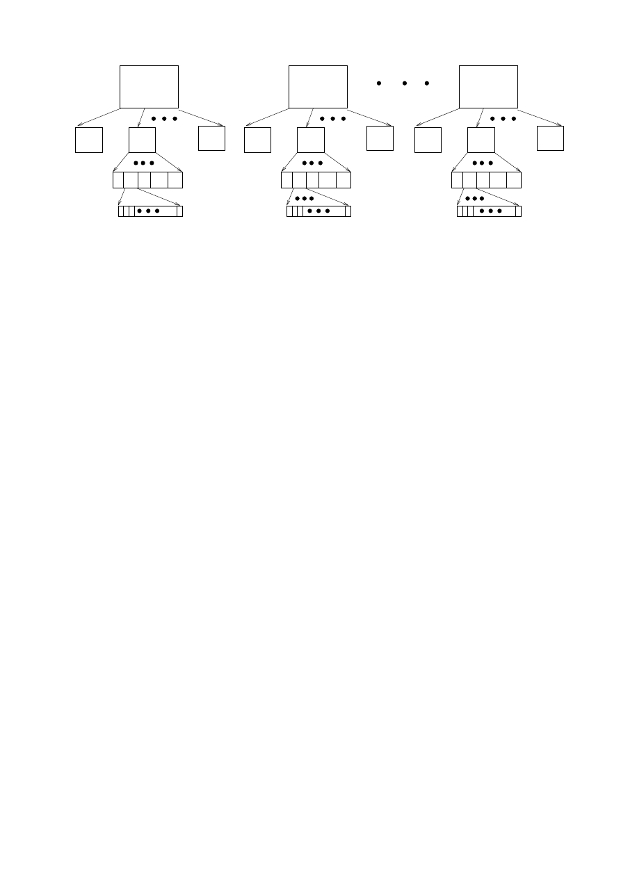
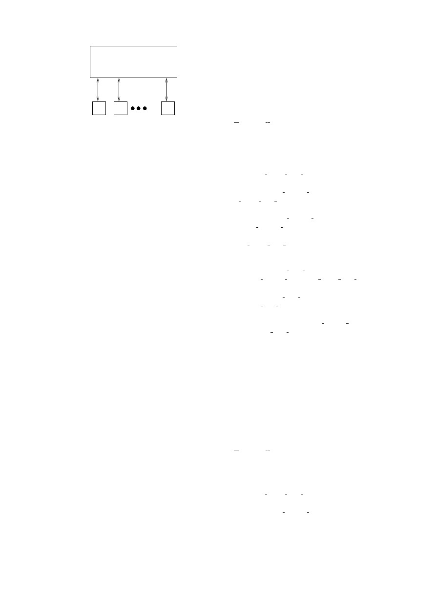
To illustrate Equations (3, 4), Figure 2 is useful. Each

of the SMs in the GPU get multiple blocks of a ker-
nel. In the picture we consider

N

B

= 8. Each of

these blocks are executed on the SM by considering
each block as a set of

N

w

warps. Each warp is then

treated as a set of

N

t

threads. It is these threads that

are essentially executed in parallel on the 8 cores of the
SM. In Figure 2, we have used

N

w

= 16 and N

t

= 32.

Unlike sequential computation, there is another ele-

ment that has an impact on the performance of GPU
programs. Multiprocessors employ time-sharing as a la-
tency hiding technique. Within the context of the GPU,
this time-sharing is in the form of each SM handling
more than one block of threads at the same time. To
model this situation and its effect, let us assume that
each SM gets

b blocks of threads that it can time-share.

Notice that when we use the MAX or the sum model
to estimate the time taken by a kernel, all the

b blocks

then require

b times the time taken by a single block.

The number of blocks assigned sequentially to an SM
N

B

effectively reduces by a factor of

b. So there is no

net effect of time sharing as long as latencies are hidden
well. So, our Equation (4) stands good even in the case
of time sharing.

3.5

A Few Reflections on the Model

At this stage we find it pertinent to discuss two issues
related to the model. The first question the reader is
likely to have is: ”Is it required to model at such a low
level where one has to count the number of cycles for
each operation?”. The performance of a CUDA kernel
can vary drastically with small changes in memory ac-
cess strategies. Using shared memory may yield up to
20 times better performance than using global memory
and using coalesced global memory accesses may re-
sult in as much as 5 times performance increase over
non-coalesced access. Arithmetic operations also have
highly varying cycle requirement such as 4 cycles for
operations like integer addition to 48 cycles for inte-
ger modulus. Any model that does not capture these
changes is unlikely to be accurate.

The second question that a reader would have is:

”How difficult is it to perform such an analysis?”. In
our view, performing such an analysis for arithmetic op-
erations would be not be significantly harder then per-
forming an asymptotic analysis. Unlike other architec-
tures the GPU does not have any sort of implicit caching
across different types of memories. Storing data in a
particular type of memory, and then, the strategy to ac-
cess it is the explicit choice of the user. As there is no
scope for issues like cache misses, analyzing memory
access patterns in our model is no easier or harder than
it is in the case of asymptotic analysis.

In the following, with the help of a carefully chosen

set of experiments, we first corroborate our model and
then proceed to case studies.

4

Corroborating the Model

We show the results of some basic experiments that cor-
roborate our model.

4.1

Coalesced/Non-coalesced Access

To understand the effect of coalesced vs. non-coalesced
memory accesses on the performance of a thread, we set
up the following simple experiment.

Experiment 1.

We set up an experiment that con-

trols how many threads in a warp can benefit from a

6

2

W

2

W

2

W

SM 1

Block 1

W

1

32 Threads

16

W

Block 2

Block 8

SM 2

Block 1

W

1

32 Threads

16

W

Block 2

Block 8

SM 30

Block 1

W

1

32 Threads

16

W

Block 2

Block 8

Figure 2: The threads in a warp are executed in parallel. Groups of warps are arranged into block and block are
assigned to SMs.

coalesced access. This is controlled by the parame-
ter

stride

in the code Listing 1. (see Appendix B).

stride

denotes the gap between the elements that are

accessed in sequence by a single thread. Hence, threads
in a half-warp can benefit from a coalesced access if the
value of

stride

is large. For example, when

s

tride

= 32, each thread of a warp gets consecutive elements,
which ensures complete coalescing. When the

stride

is 1, each thread across a warp gets elements that are
displaced by 32, hence is guaranteed to be completely
non-coalesced and requires 16 memory transactions to
be serviced for a half-warp. In order to ensure a fair
comparison, in our code, the number of accesses by a
thread is independent of

stride

.

In the code given in Listing 1, the amount of com-

putation per iteration is very small compared to the
memory access latency for

stride = 1

. However,

as we increase the value of

stride

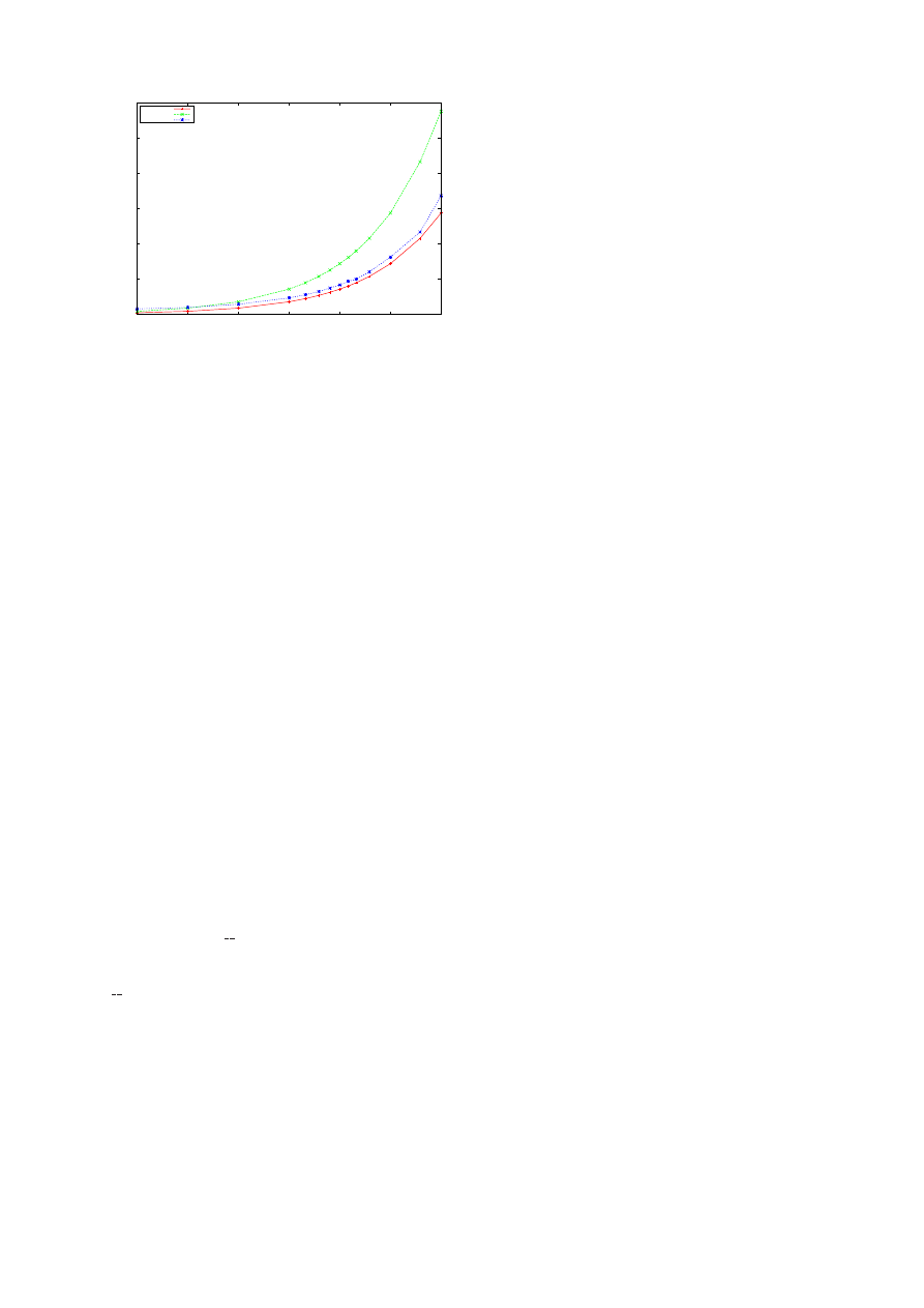
, memory access

and computation take about the same number of cycles.
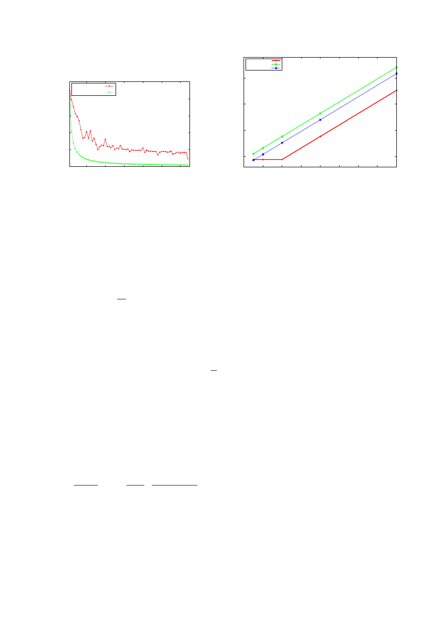
Using the MAX model, we predict the runtime of this
kernel and plot it along with the actual runtime in Fig-
ure 3(a) plots the program runtime for various values of

stride

. It must be noted that a purely memory ac-

cess base code, i.e., with little compute, is difficult to
model due to limited knowledge about the memory ac-
cess hardware.

4.2

Understanding access conflicts

To understand the validity of our model in the case of
access conflicts, we performed the following experi-
ment.

Experiment 2.

In this experiment, keeping the over-

all structure of the global accesses as in Experiment 1,
each thread now writes an element to the shared mem-
ory. The access pattern to the shared memory is con-

trolled by a variable

bank

which can be given a value

between 0 to 16. With a larger value of

bank

we can

thus increase the number of bank conflicts.

The kernel in Listing 2 (in Appendix B) has about

16 cycles of compute per iteration and there are 64000
iterations. The number of cycles required for memory is
about

bank

×4 per iteration. The actual runtime and the

runtime predicted by our model is plotted in Figure 3(b).
As can be seen, there is indeed a linear dependency on
the number of conflicts and the program runtime.

5

Case Studies

In this section, we further validate our model by con-
sidering non-trivial problems as case studies. The case
studies we consider are matrix multiplication, list rank-
ing, and histogram generation. These case studies cover
all the features of our model. The matrix multiplica-
tion kernel is compute intensive, the list ranking kernel
is global memory intensive and is a popular case study
for irregular algorithms, and the histogram case study
makes use of shared memory resulting in bank conflicts.
Hence, the choice of our case studies is justified. For
simplicity, we drop the parameter

K in quantities such

as

N

B

(K) and simply write N

B

.

5.1

Case Study 1: Matrix Multiplication

We shall start with matrix multiplication which is a
highly popular problem in parallel computing with sev-
eral applications. The algorithm considered here [4,
Chapter 6] launches one thread per element of the prod-
uct matrix

C in A × B = C. To improve data locality,

we can keep a block of rows from the matrix

A and a

block of columns from the matrix

B in the shared mem-

7

0

10

20

30

40

50

10

20

30

40

50

60

Time (ms)

Stride across iterations (words)

Actual Time

Predicted Time

(a) Effect of coalescing

500

1000

1500

2000

0

2

4

6

8

10

12

14

16

Time (ms)

No. of Bank Conflicts

MAX Time
SUM Time

Actual Time

(b) Effect of Access Conflicts

Figure 3: Studies to corroborate the model.

ory. These blocks can be multiplied to get partial re-
sults. As the access to elements in the shared memory
can be made to be non-conflicting, by choosing the ac-
cess pattern carefully [4], the algorithm benefits from
fast accesses to the shared memory as well as maintain-
ing coalesced access from global memory.

For multiplying matrices of size

N × N , the total

number of blocks is

N

2

256

with each block consisting of

N

w

= 8 warps at the rate of N

t

= 32 threads per warp.

So each SM gets

N

B

= N

2

/256 · 30 blocks.

As per the implementation above, the work done

per block/thread scales with the number of rows and
columns. The dimensions of a thread block are

16 × 16.

Each thread then loads a value from matrices

A and B

into shared memory, iteratively computes each element
of

C

sub

and writes it back to memory. This requires

N

16

iterations for each thread. The number of computation
cycles required per thread for a matrix of

N rows and

columns can be counted to be

Ncomp = 760N/16.

As each thread performs 3 global and 2 shared mem-

ory accesses, the cycles spent in memory operations in
this thread can be counted to be

Nmemory = 240N/16.

Thus, when using the MAX model, the com-

pute time dominates the memory time.

Let

C

T

=

max{Ncomp, Nmemory}. Using Equation 4, the to-
tal time required for multiplying the matrices under the
MAX model is:

N

2

256 · 30

· 8 · 32 ·

760N

16

·

1

32 × 1.3 × 10

9

At

N = 128, the estimated time using the MAX

model comes to around 11 ms which compares favor-
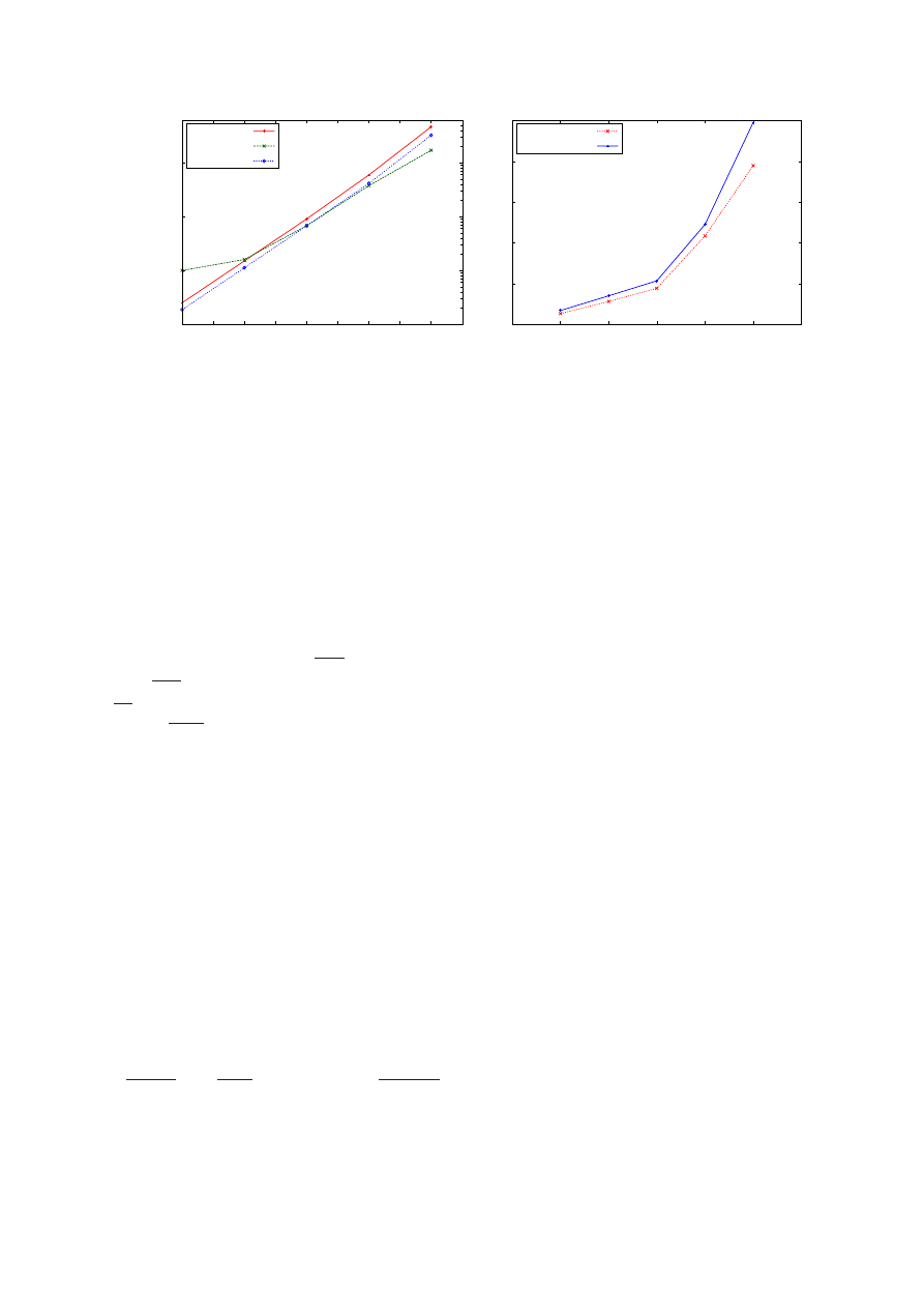
ably with the actual time of 16 ms. The predicted run

time of this algorithm for both the SUM and MAX
models for various values of

N are plotted in Figure

4(a). Matrix multiplication requires block synchroniza-
tion which is difficult to predict and hence there is a
some deviation from the actual runtime.

5.2

Case Study 2: List Ranking

In parallel computing, list ranking is one of the fun-
damental operations with applications to several prob-
lems. While list ranking does not figure at all as an im-
portant problem in sequential computing, the difficulty
of the problem in parallel computing is recognized early
by Wyllie [14]. Using various techniques, several algo-
rithms to solve this problem are proposed [12, 1, 3].

For symmetric multiprocessors, Hellman and J`aJ`a

[12] proposed an algorithm for list ranking that has
a runtime of

O(log n) with high probability when the

number of processors is small compared to the size of
the input. Their algorithm suggests that the

n/p sub-

lists are ranked locally and a list of size

n/p be ranked

sequentially. Several implementations of this algorithm
are reported on various multi-core architectures includ-
ing the most recent one on the Cell BE [2].

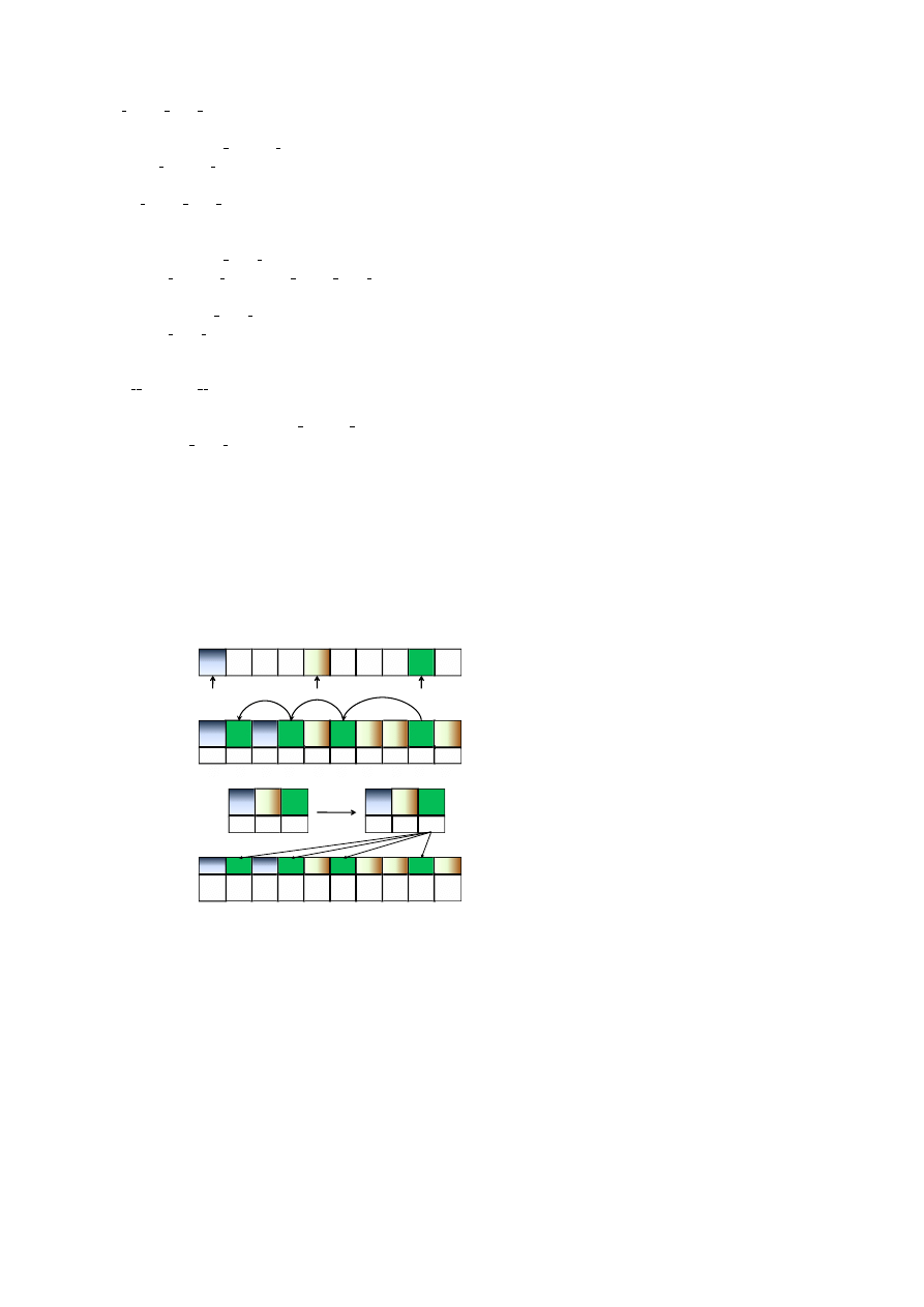
A recursive variant of the algorithm, developed for

GPU, proceeds as follows [20]. Initially,

p splitters (lo-

cal leaders) are chosen at equi-distant points in the suc-
cessor array. Using these splitters, elements of the list
are ranked locally till the next splitter is reached. Now,
recursively, the list of splitters is ranked. Finally, the
(global) ranks are computed using the local rank and
the rank of the splitter to which the element belongs.

8

0.01

0.1

1

10

12

13

14

15

16

17

18

19

20

21

Time (ms)

logarithm (no. of elements)

SUM Time

Actual Time

MAX Time

(a) Matrix Multiplication

0

5

10

15

20

25

17

18

19

20

21

22

23

Time (ms)

logarithm (list size)

Estimated Time

Actual Time

(b) List Ranking

Figure 4: Figure (a) shows the estimated and actual times of the matrix multiplication kernel on square matrices of
size

2

6

× 2

6

to

2

11

× 2

11

. Figure (b) shows the estimated and the actual time taken by the list ranking kernel on lists

of size varying from

2

18

elements to

2

22

elements.

Figure 7 (in Appendix C) shows an illustration.

In this case study, we focus on the local ranking as-

pect of the recursive variant of the Hellman-J`aJ`a [12]
algorithm. During the local ranking phase, it can be
noticed that the elements accessed each thread exhibit
no particular spatial locality. Hence, this kernel falls
under the simple model of the GPU as a PRAM with
non-coalesced accesses to the global memory.

With

N elements and p =

N

log N

splitters, we re-

quire

N

log N

threads. These threads are grouped into

N

512

blocks of 512 threads each.

Of these at most

N

B

= ⌈

N

512·30

⌉ blocks are assigned to any single SM

on the GPU. Each of these blocks consists of

N

w

= 16

warps of

N

t

= 32 threads each.

Since we are working with a random list, some

threads process more work than others.

Typically,

the most likely size of the sublist was observed to be
4 log N elements, which also confirms to known results
on probability. The memory cycles taken by a thread
can be computed as follows. Each thread involves 3
reads/writes to the global memory for each element that
this thread is traversing. All these accesses are non-
coalesced. So with about

4 log N elements per sublist,

Nmemory = 4 log N · 3 · 500. The compute in each
thread is very minimal. So we ignore this completely
and set

C

T

(K) = Nmemory.

The overall time taken by the kernel to compute the

local ranks for each sublist can then be computed using
Equation 4 as:

N

512 · 30

· 16 ·

32

8 × 4

· 4 log N · 3 · 500 ·

1

1.3 × 10

9

For

N = 2

22

we get the time per SM to be

≈ 21.0

millisecond. This compares favorably with the actual
time for this kernel for

N = 2

22

at 24 millisecond. Fig-

ure 4(b) shows the comparison of the estimate and the
actual times over various list sizes, ranging from 256 K
to 4 M elements. We note that since the computation in
each thread is very minimal to the memory access cost,
the models MAX and SUM exhibit identical behavior.
So we show only the estimates from the MAX model.

5.3

Case Study 3: Histogram Generation

Counting elements of the same category is a common

problem spreading across a wide variety of applications.
It is one of the basic primitives in the field of statistics,
image processing, and data engineering. Let

N obser-

vations be chosen independently and uniformly at ran-
dom between

1 through B, both inclusive. Let us as-

sume that these

N observations are to be placed into B

bins.

In this case study we test our model against the shared

memory access patterns. Each block loads its share
of input data one by one from the global memory in
a coalesced manner and updates the histogram in the
shared memory. When the block has gone through all
its data the shared memory histogram is copied to the
global memory in a coalesced manner. These local his-
tograms can then be added together to obtain the global
histogram. See [19] for more details. In this case study,
we only compare the estimates from our model with that
of the actual time for computing the local histograms.

9

0

1

2

3

4

5

6

1

2

4

8

16

32

64

Time (ms)

No. of Elements (in Million)

MAX
SUM

Actual

Figure 5: The estimated and the actual runtime of the
histogram kernel on various input sizes.

Obtaining the global histogram from these local his-
tograms is an easy operation and hence is omitted from
the timing analysis.

For correctness, threads in a block should compute

the local histogram of the block using atomic opera-
tions. However, our model at this point does not account
for atomic operations. Hence, for the purposes of this
case study, we let all these increment operations conflict
in the shared memory. We thus time the kernel ignoring
the correctness of the result.

In our implementation [19], each thread builds the lo-

cal histogram of

N/1920 × 256 elements into 256 bins.

This involves reading each element from the global
memory in a coalesced manner and updating the count
in the appropriate bin in the shared memory. Thus, the
amount of compute and the memory access per element
is very small.

Using the model described in Section 3, we obtained

the estimates for the runtime according to both the
MAX and the SUM variants. The actual and the esti-
mated times are plotted in Figure 5. The plot suggests
that latency hiding works very well in this kernel.

6

Limitations of Our Model

Our model however has a few drawbacks. Our model
does not consider the effect of intra-block synchroniza-
tion calls such as

syncthreads(). However, the model

can be extended for this by treating each kernel as
being composed of sub-kernels separated by calls to

syncthreads().

Our model at present does not handle atomic opera-

tions. These are to be handled by serializing the threads
participating in the atomic operation. Our early results
in this direction are encouraging, and this aspect shall
be included in the full version of the paper.

Also, we did not specifically mention the effect of

computational divergence among threads in a warp, and
atomic operations on data in global and shared memory
cells. Bringing these parameters into a future model re-
quires a better understanding of the architecture and the
scheduling aspects of the GPU.

7

Conclusions

In this paper we proposed a performance model for the
Nvidia GPU by using popular models in the parallel al-
gorithm community. Our effort is a step to bridge the
gap between the theory and practice of parallel pro-
gramming on the GPU. In future, we wish to use this
model to develop a simulator for the GPU that can ease
further architectural developments of GPGPU.

References

[1] A

NDERSON

, R. J.,

AND

M

ILLER

, G. L. A Simple Ran-

domized Parallel Algorithm for List-Ranking. Informa-
tion Processing Letters 33, 5 (1990), 269–273.

[2] B

ADER

, D. A., A

GARWAL

, V.,

AND

M

ADDURI

, K. On

the Design and Analysis of Irregular Algorithms on the
Cell Processor: A Case Study of List Ranking. In Proc.
of IEEE IPDPS (2007), pp. 1–10.

[3] C

OLE

, R.,

AND

V

ISHKIN

, U. Faster Optimal Parallel

Prefix sums and List Ranking. Information and Compu-
tation 81, 3 (1989), 334–352.

[4] C

ORPORATION

, N. CUDA: Compute Unified Device

Architecture Programming Guide. Tech. rep., 2007.

[5] C

ULLER

, D., K

ARP

, R., P

ATTERSON

, D., A. S

AHAY

,

K. E. S., S

ANTOS

, E., S

UBRAMONIAN

, R.,

AND VON

E

ICKEN

, T. LogP: Towards a Realistic Model of Parallel

Computation. In Proc. ACM PPoPP (1993), pp. 1–12.

[6] F

ORTUNE

, S.,

AND

W

YLLIE

, J. Parallelism in Random

Access Machines. In Proc. ACM STOC (1978), pp. 114–
118.

[7] G

IBBONS

, P. B., M

ATIAS

, Y.,

AND

R

AMACHAN

-

DRAN

, V. The queue-read queue-write asynchronous

pram model. In In Proc. of EURO-PAR (1996).

[8] G

IBBONS

, P. B., M

ATIAS

, Y.,

AND

R

AMACHAN

-

DRAN

, V.

The Queue-Read Queue-Write PRAM

Model: Accounting for Contention in Parallel Algo-
rithms. SIAM J. Comp. 28, 2 (1999), 733–769.

[9] G

OVINDARAJU

, N.,

AND

M

ANOCHA

, D.

Cache-

efficient Numerical Algorithms using Graphics Hard-
ware. Parallel Computing 33, 10-11 (2007), 663–684.

[10] G

UTIERREZ

, E., R

OMERO

, S., T

RENAS

, M. A.,

AND

Z

APATA

, E. L. Memory Locality Exploitation Strate-

gies for FFT on the CUDA Architecture. In Proc. of
High Performance Computing for Computational Sci-
ence - (2008), pp. 430–443.

10

[11] H

ARISH

, P.,

AND

N

ARAYANAN

, P. J.

Accelerating

Large Graph Algorithms on the GPU using CUDA. In
Proc. of HiPC (2007).

[12] H

ELMAN

, D. R.,

AND

J `

A

J `

A

, J. Designing Practical

Efficient Algorithms for Symmetric Multiprocessors. In
Proc. ALENEX (1999), pp. 37–56.

[13] H

OPF

, M.,

AND

E

RTL

, T.

Hardware Accelerated

Wavelet Transformations. In Proc. EG Symposium on
Visualization (2000), pp. 93–103.

[14] J `

A

J `

A

, J. Introduction to Parallel Algorithms. Addison-

Wesley, 1992.

[15] L

UO

, Y.,

AND

D

URAISWAMI

, R. Canny Edge Detec-

tion on Nvidia CUDA. In Proc. of IEEE Computer Vi-
sion and Pattern Recognition (2008), pp. 1–8.

[16] M

ENG

, J.,

AND

S

KADRON

, K. Performance modeling

and automatic ghost zone optimization for iterative sten-
cil loops on gpus. In Proc. of ACM ICS (2009).

[17] N

GUYEN

, H. GPU Gems 3. Addison-Wesley Profes-

sional, 2007.

[18] N

ICKOLLS

, J., B

UCK

, I., G

ARLAND

, M.,

AND

S

KADRON

, K.

Scalable Parallel Programming with

CUDA. ACM Queue 6, 2 (2008), 40–53.

[19] P

ATIDAR

, S.,

AND

N

ARAYANAN

, P. J. Scalable split

and gather primitives for the gpu. Tech. rep., 2009.

[20] R

EHMAN

,

M.

S.,

K

OTHAPALLI

,

K.,

AND

N

ARAYANAN

, P. J.

Fast and Scalable List Rank-

ing on the GPU. In Proc. of ACM ICS (2009).

[21] R

YOO

, S., R

ODRIGUES

, C. I., S

TONE

, S., B

AGH

-

SORKHI

, S. S., U

ENG

, S.-Z., S

TRATTON

, J. A.,

AND

H

WU

, W. W. Program Optimization Space Pruning for a

Multithreaded GPU. In Proc. the Intl. Symp. Code Gen.
and Opt. (2008), pp. 195–204.

[22] S

CHAA

, D.,

AND

K

AELI

, D. Exploring the multiple-

gpu design space. In Proc. of the IEEE (IPDPS) (2009).

[23] S

ENGUPTA

, S., H

ARRIS

, M., Z

HANG

, Y.,

AND

O

WENS

, J. D. Scan Primitives for GPU Computing. In

Proc. ACM Symp. Graphics Hardware (2007), pp. 97–
106.

[24] V

ALIANT

, L. G. A Bridging Model for Parallel Com-

putation. Comm. ACM 33, 8 (1990), 103 – 111.

[25] V

INEET

, V.,

AND

N

ARAYANAN

, P. J. CUDA Cuts: Fast

Graph Cuts on the GPU. In Proceedings of the CVPR
Workshop on Visual Computer Vision on GPUs (2008).

[26] V

IOLA

, I., K

ANITSAR

, A.,

AND

G

ROLLER

, E.

Hardware-Based Nonlinear Filtering and Segmentation
using High-Level Shading Languages. In Proc. IEEE
Visualization (2003), pp. 309–316.

A

A Brief Review of the BSP,
PRAM, and QRQW Models

In this section, we attempt a short review of the three
models of parallel computation that we use in our work.

A.1

The BSP Model

Valiant [24] proposed a bridging model called the Bulk
Synchronous Parallel (BSP) model that aimed to bring
together hardware and software practitioners.

The

model, which Valiant [24] shows can be easily realized
also in hardware existing at that time, has three main
parameters:

• A number of components that can perform compu-

tation and memory accesses;

• A router that transfers messages between compo-

nents; and

• A facility for synchronizing all (or a subset) of the

components at regular intervals of

L time units. L

is also called as the periodicity parameter.

Valiant suggests hashing to distribute memory ac-

cesses uniformly across the components. The perfor-
mance of a router is captured by its ability to route

h-

relations, where each component is the source and the
destination of at most

h messages. Using the model one

can then state the runtime of a parallel program in terms
of the parameters

L, p, g, and the input size n. In the

above,

p refers to the number of (physical) processors

and

g is the time taken by the router to route a permu-

tation. The key idea of the model is to find a value of

L

so that optimality of runtime can be achieved, i.e., truly
balance the local computation with message exchange
time.

A.2

The PRAM Model

The PRAM model of parallel computation is a natu-
ral extension of the von Neumann model of sequential
computation. Consider a set of processors each with
a unique identifier called a processor index or proces-
sor number. Each processor is equipped with a local
memory. Moreover, the processors can communicate
with each other by exchanging data via a shared mem-
ory. Shared memory is sometimes also referred to as
global memory. A schematic is shown in Figure 6. It
is often also assumed that the processors operate in a
synchronous manner. This model is called the PRAM
(Parallel Random Access Memory) model.

Naturally, when the memory is shared between pro-

cessors there can be contention for concurrent reads and

11

1

P

2

P

n

P

Shared Memory

Figure 6: Model of a PRAM.

writes. Depending on whether they are allowed or not,
several variants of the PRAM model are possible with
rules for resolving concurrent writes. In the Exclusive
Read Exclusive Write (EREW) PRAM, any concurrent
reads/writes are forbidden. In the Concurrent Read Ex-
clusive Write (CREW) PRAM, concurrent reads are al-
lowed but concurrent writes are forbidden. In the most
powerful model, the Concurrent Read Concurrent Write
(CRCW) PRAM, concurrent reads and writes are al-
lowed. Special semantics are needed to handle concur-
rent writes.

A.3

The QRQW Model

To offset the limitation of the PRAM model to han-
dle memory contentions and their effect on the per-
formance of a parallel program, Gibbons, Matias, and
Ramachandran [8] introduced the Queue-Read-Queue-
Write (QRQW) model. Here, in its simplest form, pro-
cessors are allowed to contend for reading and writ-
ing at the same time. Contending accesses are queued.
This, this model falls in between the Exclusive Read
Exclusive Write (EREW) PRAM and the Concurrent
Read Concurrent Write (CRCW) PRAM. The advan-
tage of this model becomes clear when one sees that the
EREW model of the PRAM is too strict and the CRCW
model of the PRAM is too powerful. Hence, the QRQW
model tries to separate the highly contentious accesses
and accesses with very low contention. Most hardware
realizations can support the latter better than the for-
mer. Moreover, it is observed that most existing ma-
chine models behave in a QRQW fashion.

In its general form, the model can also work with

a contention function

f (.) that governs contentious ac-

cesses to the memory. While

f being a linear function,

we get the QRQW PRAM and, for example,

f (i) = ∞

for

i > 1 and f (1) = 1 is the EREW PRAM. The work

of [8] studies variants such as synchronous and asyn-
chronous QRQW PRAM.

B

Code Listing

B.1

Code for understanding the effect of
coalescing

#define STRIDE

32

#define OFFSET

0

global

void

coalesing(

float

*a,

int

N)

{

//Calculate Thread Start, End and

Stride

int

n elem per thread = N /

(gridDim.x * blockDim.x);

int

block start idx =

n elem per thread * blockIdx.x *
blockDim.x;

int

thread start idx =

block start idx

+ (threadIdx.x / STRIDE)

* n elem per thread * STRIDE

+ ((threadIdx.x +

OFFSET) % STRIDE);

int

thread end idx =

thread start idx + n elem per thread

* STRIDE;

if

(thread end idx

>

N)

thread end idx = N;

for

(

int

idx=thread start idx; idx

<

thread end idx; idx+=STRIDE)

{

a[idx] = a[idx] + a[idx];

}

}

B.2

Code for understanding Access Con-
flicts

#define STRIDE

6

#define OFFSET

0

#define BANK

1

global

void

conflicts(

float

*a,

int

N)

{

//Calculate Thread Start, End and

Stride

int

n elem per thread = N /

(gridDim.x * blockDim.x);

int

block start idx =

12

n elem per thread * blockIdx.x *
blockDim.x;

int

thread start idx =

block start idx

+ (threadIdx.x / STRIDE)

* n elem per thread * STRIDE

+ ((threadIdx.x +

OFFSET) % STRIDE);

int

thread end idx =

thread start idx + n elem per thread

* STRIDE;

if

(thread end idx

>

N)

thread end idx = N;

//Shared Memory Declaration

shared

int

S[

512

];

for

(

int

idx=thread start idx; idx

<

thread end idx; idx+=STRIDE)

{

for

(

int

i=

0

;i

<

10000

;i++)

S[(threadIdx.x*BANK)%

512

]=a[idx];

}

}

C

List Ranking Illustration

0

1

2

3

4

5

6

7

8

9

4

8

1

3

7

-

6

2

9

5

0

3

1

2

0

1

2

3

0

1

8

3

1

4

6

7

-

2

1

-

0

4

2

2

1

-

0

6

2

0

3

0

2

5

9

2

1

0

1

2

3

1

0

5

1

4

6

3

8

9

2

7

Successor

Array

Local Ranks

New List

Successor Array

Global Ranks

Rank

Local Ranks

Final Ranks

After Ranking

(a)

(b)

(c)

(d)

Add 2

Figure 7: Illustration of the recursive Hellman-J`aJ`a al-
gorithm. The picture is reproduced from [20].

13