Anatomy of a Market Crash: A Market

Microstructure Analysis of the Turkish

Overnight Liquidity Crisis

∗

J´

on Dan´ıelsson

London School of Economics

Burak Salto˘

glu

Marmara University

June 2003

Abstract

An order flow model, where the coded identity of the counterparties
of every trade is known, hence providing institution level order flow, is
applied to both stable and crisis periods in a large and liquid overnight
repo market in an emerging market economy. Institution level order
flow is much more informative than cross sectionally aggregated or-
der flow. The informativeness of institution level order flow increases
with financial instability, with considerable heterogeneity in the yield
impact across institutions.

JEL: F3, G1, D8. Keywords: order flow model, financial crisis, in-
stitution identity, Turkey

∗

We thank Amil Dasgupta, Jan Duesing, Gabriele Galati, Charles Goodhart, Junhui

Luo, Andrew Patton, Dagfinn Rimes, Jean–Pierre Zigrand, the editor, and an anonymous
referee for valuable comments. We are grateful to the Istanbul Stock Exchange for provid-
ing some of the data. Corresponding author J´

on Dan´ıelsson, Department of Accounting

and Finance, London School of Economics, Houghton Street London, WC2A 2AE, U.K.
[e-mail], tel. [phone]. Our papers can be downloaded from
www.RiskResearch.org.

1

Introduction

A liquidity crisis hit Turkey in November 2000. At its peak, annual inter-
est rates reached 2000% overnight. The crisis was short lived, but had far
reaching implications for the Turkish financial system. Our objective is to
analyze the crisis episode with empirical market microstructure methods,
making use of an unique dataset containing details of each transaction in the
overnight repo market, including coded institutional identities. This enables
us to explicitly document the impact of individual trading strategies on the
crisis.

Traditional methods for analyzing financial crisis focus on macroeconomic
explanations, making use of low frequency macro variables, thus mostly ig-
noring factors such as institutional structures and the trading of financial
assets. In contrast, empirical market microstructure provides an efficient
framework for analyzing price formation and informational linkages in finan-
cial markets. Applied to financial crises, market microstructure methods
emphasize decision making at the most detailed level, providing a play–by–
play level analysis of how a crisis progresses. Our main investigative tool is
an order flow

1

model, enabling us to explore the impact of individual trading

strategies on yields. Order flow models have had considerable success in ex-
plaining price changes in developed markets,

2

but we are not aware of any

applications of order flow models to emerging markets crisis.

Most applications of order flow models focus on price determination with
aggregate order flow, i.e. the sum total flow from market borrow and lend
orders, separately. An exception is Fan and Lyons (2000) who study the price
impact of individual flows from several different categories of institutions and

1

Borrow (buy) order flow is the total transaction volume in a given time period for

trades when a market borrow order was used. Lend (sell) order flow is defined analo-
gously. In defining order flow one must distinguish between borrower and lender initiated
transactions. While every trade consummated in a market has both a lender and a bor-
rower, the important member of this pair is the aggressive trader, the individual actively
wishing to transact at another agent’s prices. The convention in the order flow literature
is to use the terms buy and sell, while for repos the terminology is e.g. borrow/lend,
take/give, long/short. In this paper we use the repo terminology, and use borrow/lend
instead of buy/sell.

2

Initially with equities (see e.g. Hasbrouck, 1991), and foreign exchange (see e.g. Evans

and Lyons, 2002). Recently several market microstructure studies focus on fixed income
markets, primarily U.S. Treasuries, e.g. Fleming (2001), Cohen and Shin (2002), and
Brandt and Kavajecz (2002), while Hartmann et al. (2001) study the microstructure of
the overnight Euro money market. A few empirical market microstructure studies of
US financial crises are available, e.g., Blume et al. (1989) who consider the relationship
between order imbalances and stock prices in the 1987 crash.

2

Furfine (2002) who analyzes US interbank payment flows, knowing the ex-
posure of each bank to every other bank. Several authors make use of data
sets containing limited information about institutional identities, e.g. the
Olsen HFDF93 indicative quote dataset containing the identity of quoting
institutions in FX markets. Peiers (1997) and de Jong et al. (2001) use the
HFDF93 data to study the leadership hypothesis of Goodhart (1988), while
Covrig and Melvin (2002) examine with similar data whether Japanese or
foreign banks are more informed when trading USD/YEN, and Hasbrouck
(1995) analyzes the price discovery process on related financial equity mar-
kets. Most of these models are based on the notion of efficient martingale
prices, where a risk neutral institution observes a noisy signal of the “true”
price process. This is rooted in asset price theories where the noisy signal
represents information. This modelling approach is not directly applicable to
the study of overnight liquidity; the yields are not martingales, the institu-
tions are not necessarily risk neutral, and the order flow not only represents
information about fundamentals and portfolio shifts, but also the individual
demand and supply functions for liquidity.

Our data derives from the Turkish overnight repo market, spanning most
of the year 2000. The overnight repos are traded on the Istanbul stock
exchange (ISE), an electronic closed limit order system, where credit risk
is minimal. The data set contains detailed information on each transaction
in the sample period, i.e. whether the transaction was a market borrow or
market lend, the annual interest rate, quantity, and most importantly the
coded identity of the counterparties. We therefore identify four key variables
measuring each financial institution’s trading activity: borrowing volume
split into volume from market orders and transacted limit orders, ditto for
the lending volume. We term this institution level order flow, in contrast to
cross sectionally aggregate order flow.

We estimate our model at two levels of temporal aggregation, daily and five–
minute. We observe a structural break about ten days prior to the main crisis
day, on day 225 (Nov 20), and therefore split the sample into two subsamples:
the stable period on days 1–224 (Jan 4 to Nov 17), and the crisis period
spanning days 225–240. It might be of interest to also consider the post crisis
time period, however that would not be a realistic control case: The post
crisis period includes the Christmas holidays, when trading was very sparse.
Furthermore, subsequent to the crisis, several important financial institutions
were taken over by the authorities, including the biggest purchaser of repos,
while at the same time the government was actively attempting to stabilize
the market.

The model is estimated over the full sample at the daily frequency, while the

3

five–minute frequency model is estimated separately for each subsample. We
employ three different model specifications: interest rate changes regressed
on own lags, aggregate order flow, or institution level order flow.

We obtain the following main results:

Result A Aggregate order flow is a significant but small determinant of

overnight interest rates, with less explanatory power during
the crisis than when markets are more stable

Result B Transacted limit order flow has a significant impact on interest

rate changes. Its yield impact is generally different than the
yield impact of market order flow

Result C Institution level order flow has much higher explanatory power

than aggregate order flow, its coefficients are generally of the
expected sign, and demonstrate considerable heterogeneity

Result D Institution level order flow is much more informative during

the crisis than when markets are more stable

The aggregate order flow results are generally consistent with conclusions
from empirical microstructure studies and theories of informed trading (see
e.g. O’Hara, 1994; Lyons, 2001). There are however important differences
between the overnight liquidity markets and the better studied equity and
foreign exchange markets, suggesting that most standard theories of market
maker and limit order markets do not fully reflect the market structure in our
case. These differences relate to the type of asset, and how it is traded. In
our case the asset is generally only traded once, and then consumed, where
the individual supply/demand functions for liquidity play an important role
in determining trading strategies. Both our statistical analysis and local
news accounts suggest that some borrowers were desperate for liquidity, es-
pecially during the crisis, when not being able to borrow may have resulted
in bankruptcy. In contrast, the lenders had more elastic supply functions,
implying that they had the market power, especially if they colluded in the
runup to the crisis, as was claimed by the local press.

Aggregate order flow is a small but significant determinant of interest rate
changes, more so at higher temporal aggregation levels but less during the
crisis, suggesting that the informativeness of aggregate order flow decreases
with financial instability and higher sampling frequencies. We find that insti-
tution level order flow is a much stronger determinant of interest rates than
aggregate order flow, regardless of time aggregation and the degree of finan-
cial stability. Furthermore, while the informativeness of aggregate order flow

4

decreases in the crisis period, the informativeness of institution level order
flow increases during the crisis, when it explains 52% of interest rate changes.
In most cases, the institution level regression coefficients have the expected
signs and are significant. There is considerable heterogeneity in the yield
impact of institution level order flow, both between different institutions and
market and limit orders. Some institutions are yield takers, i.e. their trad-
ing does not affect the interest rates much, whilst others have a significant
impact on yield. In some cases there is a considerable difference in the yield
impact of an institution’s limit and market orders. The order flow of some
institutions is highly predictable, while for others the predictability is lower.
In general, order flow predictability decreases during the crisis but its yield
impact increases.

Lend order flow is decreasing throughout the latter part of the sample, while
borrow order flow first increases and then starts to drop few days prior to the
crisis. We would expect this e.g. if good credits are able to lock into longer–
term funding. Since the order book is closed, and banks only learn of the
identity of their counterparties after a trade, the high informativeness of in-
stitution level order flow suggests this is a well informed market. Institution
level order flow depends on the positions held by a bank and its institu-
tional customers and trends in the personal and corporate lending books.
It can be expected to be heavily serially correlated, with highly persistent
demand/supply schedules. An institution with a big funding requirement
today is likely to have a big funding requirement tomorrow. By aggregat-
ing order flow information across institutions, we loose an essential part of
the picture by disregarding the asymmetry in the informativeness of differ-
ent institutions, especially because of the heterogeneity in the elasticities of
supply/demand. There is considerable heterogeneity in the trading strate-
gies and degree of price leadership across the various institutions, and limit
orders have a significant but different degree of informativeness from market
orders. This is especially prevalent during the crisis, when other factors, such
as fundamentals and portfolio shifts, became relatively less relevant for price
determination, causing lower informativeness of aggregate order flow during
the crisis.

These results also underscore the relevance of market microstructure in the
analysis of financial crisis. Macroeconomic analysis, focussing on low fre-
quency variables such trade balances, GDP, inflation, and central bank re-
serves, is likely to miss the salient features of the crisis. On a macroeconomic
timescale the crisis happens in a blink of an eye. The 2000 Turkish crisis
played out in the financial markets. Arguably, individual trading strate-
gies, and not macroeconomic fundamentals were the main direct cause of

5

the crisis. Market microstructure analysis provides here the missing pieces
of the puzzle, providing guidelines to national supervisors and supranational
organizations in the design of robust financial architectures.

2

Crisis, Market Structure, Data, and Infor-
mation

The main visible impact of the 2000 Turkish financial crisis was in the
overnight money market. The effect on other markets, longer maturity in-
terest rates, foreign exchange, and equities was relatively minor in relation.
Essentially, the crisis was about supply and demand of overnight liquidity.

2.1

Crisis

Turkey has a long history of financial instability.

3

Inflation was high through-

out the 1990s, close to 100%. Turkey signed its 16

th

standby agreement with

the IMF at the end of 1999, stipulating the maintenance of price levels, with
exchange rates to be determined by a crawling peg, leaving interest rates
floating. The government could not intervene in the overnight money mar-
ket as a condition of its IMF mandate.

As a part of the restructuring program the short foreign currency positions
of Turkish banks were to be limited to 20% of their total assets. Many banks,
however, exceeded this ceiling by using “off–balance sheet” transactions and
various derivative instruments, often using local bonds or Eurobonds as col-
lateral. If the value of the collateral drops, as when domestic yields increased
in the latter part of 2000, banks face margin calls. When some of the off–
balance sheet deals went against the banks, they often used the overnight
market as a source of funds to cover the resulting margin calls, leading to
increasing yields, particularly at the shortest end of the yield curve. This in
turn, caused difficulties for banks speculating on the yield curve, and a drop
in the value of the collateral, further fuelling demand for overnight liquid-
ity. Effectively, a vicious feedback loop between short yield increases, margin
calls, and short liquidity demand was formed.

Several large financial institutions started running into serious difficulties in
the second half of 2000, partly as a result of a yield curve inversion. Some of

3

See

e.g.

(see

e.g.

Eichengreen,

2001)

and

www.nber.org/crisis/turkey

agenda.html.

6

these banks were effectively starving off bankruptcy by borrowing overnight
including the largest borrower in the overnight market, Demirbank. This was
a key factor in fuelling rapid increases in liquidity demand, especially late
in 2000, and is the main reason for why the demand for liquidity was very
inelastic for many institutions. Neither the supervisors, the IMF, nor the
rating agencies seem to have taken much notice of these events, indeed, the
resulting crisis apparently took most interested parties by complete surprise.

Banks experiencing difficulties started to dump assets, contributing to a
sharp stock market drop, including Demirbank who tried unsuccessfully to
sell its 3 and 9 month Tbills in November. The government tried to “talk
down” the crisis and the IMF signalled its support. This was not successful.
Rumors started to spread in the local financial community in late November
claiming some banks were close to fail. At the same time solvent local banks
started to limit their exposure to banks rumored to be in trouble. Towards
the end of November, many foreign creditors withdrew their credit lines, and
along with solvent domestic investors, sold the domestic currency, leading to
a rapid capital outflow, starting November 22. The Central Bank (CB) pro-
vided some liquidity to the market, (but it did not intervene in the overnight
repo market), inadvertently promoting additional demand for foreign cur-
rency. Subsequently, the CB stopped providing liquidity on Nov 30, 2000.
The ever increasing demand for overnight money, fuelled rapidly increasing
yields, culminated on December 1 when the overnight interest rate reached
its peak at (simple annual) 2000%. That day local newspapers claimed the
liquidity shortage triggering the crisis was caused by large banks deliberately
withholding liquidity from the market in order to squeeze Demirbank.

Total capital outflow during this period reached an estimated USD 6 bil-
lion, eroding approximately 25% of the foreign exchange reserves of the Cen-
tral Bank. This led to an IMF emergency loan announced on Dec 5. This
briefly stabilized the economy, however uncertainty remained and financial
bankruptcies continued. (See the Chronicle of the Crisis in the Appendix for
an overview of crisis events, and the role played by the largest borrower of
overnight money, Demirbank)

2.2

Market Structure

The Bonds and Bills Market which works under the Istanbul Stock Exchange
(ISE) is the only organized, semi–automated market for both outright pur-
chases and sales and repo/reverse repo transactions in Turkey. The average
daily volume of overnight repo transactions exceeded 3 Billion USD in the

7

sample period. Financial institutions communicate their orders via telephone
to ISE staff who act as blind brokers. The repo market operates on a multi-
ple price–continuous trading system. All orders are continuously entered into
the computer system and the orders

4

automatically matched. Members are

subsequently informed about the executed transaction.

5

In order to trade on

the ISE, member institutions need to provide collateral in the form of Tbills.
If this collateral is eroded institutions can no longer trade. Historically, prac-
tically no institution has defaulted on ISE trading obligations, and traders
in ISE consider counterparty credit risk to be negligible.

Traders do not know the identity of counterparties prior to trading, and other
traders do not know that the trade took place, except by observing that a
particular limit order has vanished from the screen. Market participants
have a choice of either limit quotes or market orders, with a minimum quote
size of 5

×10

11

Turkish Liras (TRL). The limit orders are one–sided, i.e.,

traders either enter lend or borrow quotes where these quotes are firm in the
sense that the quoting institution is committed to lend/borrow until it either
withdraws the quote or another institution hits the limit order with a market
order. Each trader sees the five best bid/ask limits. The actual deal finalizes
at 4:30 pm, i.e. the daily deals settle just at the end of same day at 4:30
pm. Transaction costs for overnight repos are 0.00075%. Trading takes place
between 10 am and 2 pm with a one hour lunch break. (See Figure 5 for a
plot of the intra day seasonality pattern). For details see the ISE factbook
at website www.ise.gov.tr.

In addition to the organized market, an informal market based on Reuters
quotes exists.

Since the institution level identities of indicative Reuters

quotes is known, it serves as an important source of information. How-
ever, as in many other markets indicative Reuters quotes tend to be a form
of advertising with the actual quotes containing little information (see e.g.
Dan´ıelsson and Payne, 2002). Finally, some trading takes place at the Cen-
tral Bank. While the exact volume in these two latter markets is unknown
(it does not appear to be recorded), it is assumed by market participants to

4

Bid orders are matched with equal or lower priced ask orders and ask orders are

matched with equal or higher priced bid orders

5

Various tasks such as daily marking-to-market of securities (government bonds, trea-

sury bills) during the validity period of the repo transaction, computing margin excess
deficit automatically and making margin calls if necessary, and ensuring securities and
cash transfers at the close of the transaction are performed by the ISE Bonds and Bill
Market and Settlement and Custody Bank Inc. (Takasbank). However, clearing and set-
tlement operations are handled by the ISE Settlement and Custody Bank Inc., which
is the institution inaugurated by the ISE and its members and institution safekeeps the
underlying securities.

8

be much smaller than the organized market.

2.3

Data

The dataset contains details of all transactions in the overnight repo market
for 240 days from the beginning of year 2000 (Jan 4) to Dec 11. During this
period, 256,141 transactions are recorded. For each transaction we know the
interest rate, volume, and whether the trade was borrow or lend initiated,
providing signed order flow. Furthermore, we know the coded institutional
identity of the counterparties in each trade, enabling us to identify the in-
stitution level order flow, see Section 3.1. The sample contains 136 different
financial institutions.

The main crisis occurs on day 234 (Dec 1). Statistical analysis of the data
and newspaper accounts of the crisis indicate that the buildup to the crisis
starts a few days earlier. Effectively, we observe a structural break about
ten days prior, around day 225 (Nov 20) suggesting that it is necessary to
estimate the model separately for each of the two periods. As a result, we
split the data up into two main subsamples: days 1 to 224 referred to as the
stable period, and days 225 to 240 referred to as the crisis period.

2.4

Information Available to Market Participants

Information is at the heart of market microstructure analysis, see e.g. Easley
and O’Hara (1987), O’Hara (1994), and Lyons (2001). In the Turkish market,
several channels of information are open to market participants.

First, large local banks have extensive dealings with big foreign banks, im-
plying that the local actions of foreign banks can be inferred by their local
counterparties. Second, institutions know the identity of their own coun-
terparties after executing trades, and therefore observe whether the trading
patterns of their counterparties are unusual. The third information source
is Reuters indicative quotes, where the identity of quoting institutions is
known. While the accuracy of the indicative quotes, especially the spread, is
likely to decrease during the crisis, it may still be a valuable source of infor-
mation, at least by providing the identities of quoting institutions. Fourth,
indirect information channels, (traders gossip, news, etc.) are very active in
the Turkish market. Finally, observing interest rate movements, both in the
overnight market as well as on longer maturities provides valuable insights
to traders. For example, a large yield drop for long maturity bonds, cou-
pled with a large yield increase in the overnight market may suggest that

9

institutions speculating on the yield curve are experiencing difficulties. By
combining these information sources it is possible for market participants
to get a fairly accurate picture of market activity. Hence, the information
content of institution level order flow has the potential to be considerable.

3

Model Specifications

Order flow affects asset prices because it conveys information, (see e.g. O’Hara,
1994; Lyons, 2001, for an overview). In their preference for limit or market
orders, traders reveal their private information. In such models, sell market
orders reflect selling pressure, and buy market orders buying pressure. Typ-
ically, the underlying asset is assumed to follow a martingale process, where
order flow helps in explaining contemporaneous price movements, but does
not forecast asset price movements. Most order flow models focus on market
orders, since in the absence of other information, limit order flow is simply
the reverse of market order flow.

Order flow models have been successfully applied to equity markets (see e.g.
Hasbrouck, 1991), foreign exchange markets (see e.g. Evans and Lyons, 2002),
and fixed income markets (see e.g. Brandt and Kavajecz, 2002). They are
typically found to have considerable explanatory power when measured by
R

2

, often in the range of 40% to 60% as in the Evans and Lyons (2002)

study of daily exchange rates. However, Brandt and Kavajecz (2002) find
much lower

R

2

for order flow models when applied to the lowest maturity

US government bonds.

In constructing our model we need to take into account several unique fea-
tures of the overnight repo market and the Turkish economic situation.

1. Turkey is an emerging markets economy, with a small number of large

market players and light supervision.

2. Overnight repos represent liquidity which is needed for the regular run-

ning of the banking system. It can be very costly for individual insti-
tutions not to obtain this liquidity. Most financial institutions in this
market trade for liquidity reasons and not for speculative reasons.

3. The overnight repo has a lifetime of one trading day. Throughout

the trading day market participants are trading an asset that only
exchanges hands after trading ceases. Since a one day repo today is
not the same asset as a one day repo tomorrow, the observed prices
over time are prices of the same units of different assets. Most market

10

participants trade only on one side of the market, i.e they either borrow
or lend, but not both.

4. We can not assume the repos follow a martingale process, e.g. because

of the short life time of the asset. For most other types of assets,
the underlying price process is a martingale whereby the asset price
reflects fundamentals or the intrinsic value of the asset, with market
efficiency ensuring random walk. Here, after first being traded, the
asset is generally not traded again, but consumed. The yields therefore
reflect the price of a diminishing quantity of supply, with the agents
supply and demand functions determining the price. As a consequence,
order flow reflects the short term demand and supply for liquidity, above
and beyond the impact of portfolio shifts and fundamentals.

These features of the overnight repo markets and the specific situation in
Turkey imply that the theoretic environment of the one day repo market
differs from better known equity and foreign exchange markets, and longer
maturity fixed–income markets. While market efficiency dictates that such
market prices cannot be forecasted with either own lags or lagged order flow,
this is not the case for one day repos. The trading volume of individual insti-
tutions is predictable due to persistence in demand/supply needs, implying
that both order flow and interest rates can be forecasted to some extent.

It is beyond the scope of this paper to develop and test theories about trading
in overnight liquidity markets. Instead, we focus on establishing empirical
stylized facts. To this end we consider three different model specifications,
where interest rate changes are regressed on own lags, aggregate order flow,
or institution level order flow. The models are estimated at both daily and
five–minute frequencies where the daily model covers the entire data sample
whilst the five–minute model is estimated for the crisis and stable periods
separately, i.e. days 1–224 and 225–240. We use two main diagnostic tools.
First, the explanatory power of the models is measured by centered

R

2

.

Second, we gauge the importance of institution level order flow by recording
parameter values, signs, and significance.

3.1

Notation

We use three types of variables in our analysis, interest rates, aggregate or-
der flow, and institution level order flow. Most empirical order flow models
use changes in asset prices as the dependent variable, implying a linear rela-
tionship between order flow and prices. In our case, this is not a reasonable

11

assumption because of the extreme differences between price changes in the
stable and crisis periods. Hence, we use log interest rate differences, where
order flow affects relative and not absolute rate changes. The interest rate
variable,

R

t

, records the last observation in each time interval. For the daily

data it is the closing interest rate, and for the five–minute aggregated data
it is the last observation in each interval. Hence, the dependent variable is
∆

r

t

≡ log R

t

− log R

t−1

.

Borrow order flow,

b

t

, is defined as the sum of transaction volume from

market borrow orders over the time interval. If

v

τ

is the transacted volume

of trade at time

τ, and ι

τ

is an indicator variable that takes the value one if

the trade at time

τ was a market borrow, and zero otherwise, then

b

t

≡

τ

v

τ

ι

τ

, t − 1 ≤ τ < t.

The definition of lend order flow,

l

t

, is equivalent.

The data sample contains observations on 136 different financial institutions,
where each institution is known by a random identity code, i.e., a number
between 0 and 135. For each transaction, we know the identity code of both
counterparties and whether each transaction was lender or borrower initiated,
i.e., if the market order was a lend or borrow. For each institution we know
its borrow volume and sell volume and whether the volume results from the
institutions market orders or executed limit orders. Note that this is not
the limit order flow, only limit orders resulting in a transaction in the time
interval. As a result we record four separate variables for each institution

i

in the time interval

t − 1 to t:

Financial institution

i

volume split into

borrow volume

from

lend volume

from

its market

orders

b

m

t

(

i)

its executed

limit orders

b

l

t

(

i)

its market

orders

l

m

t

(

i)

its executed

limit orders

l

l

t

(

i)

Hence, the

b() and l() signals the institutions borrowing and lending, while

12

m

indicates the institution flow from market orders, and

l

is the flow from its

executed limit orders. (

i) identifies the institution.

We define the entire vector of institution level order flow as:

W

t

≡






b

m

t

(0)

l

l

t

(0)

b

l

t

(0)

l

m

t

(0)

..

.

..

.

..

.

..

.

b

m

t

(135)

l

l

t

(135)

b

l

t

(135)

l

m

t

(135)






Since we only use a subset of the institution level order flow, we denote

W as

the matrix of the institution level order flows that are used in the estimation.

3.2

Models

3.2.1

Interest Rate Model

The baseline interest rate model is a regression of interest rate changes on
own lags.

∆

r

t

= log(

R

t

)

− log(R

t−1

) =

c + α

N

(

L)∆r

t−1

+

t

(1)

where

R

t

is the repo rate,

c is a constant,

N

(

L) is the lag operator with N

lags, and

t

is a white noise innovation term.

3.2.2

Aggregate Order Flow Model

In the standard order flow model price changes are regressed on net order
flow, i.e. buy minus sell flow, see e.g. Hasbrouck (1991) and Evans and
Lyons (2002). This is a reasonable assumption when buy and sell order flow
are assumed to be equally informative, as in the foreign exchange markets.
Several authors studying equity markets, e.g. Harris and Hasbrouck (1996)
and Lo et al. (2002) suggest that the informativeness of buy and sell order
flow might not be equal. In our case not only are the statistical properties of
borrow and lend order flow significantly different, see Tables 1 and 2, in most
cases the financial institutions are either lenders or borrowers, not both.

Given the relationship between order flow and interest rate changes, includ-
ing lagged order flow also captures some of the information in lagged rate
changes, without increasing the number of parameters to be estimated. We
hence exclude lagged interest rate changes from the model.

∆

r

t

=

c + β

N

(

L)b

t

+

δ

N

(

L)l

t

+

t

.

(2)

13

where

b is borrow order flow and l lend order flow.

3.2.3

Institution Level Order Flow

We are not aware of any published empirical market microstructure studies
where the institutional identities of the counterparties of every transaction
are known. However, several authors have analyzed price formation when
some information about the identity of individual institutions is available,
typically indicative quotes in foreign exchange markets. Many such studies
use the Olsen HFDF93 dataset, e.g. Peiers (1997) and de Jong et al. (2001),
while Covrig and Melvin (2002) consider whether Japanese or foreign banks
are more informed while trading YEN/USD, and Wei and Kim (1997) use
data on the foreign currency positions of large market participants. Alter-
natively, Hasbrouck (1995) analyzes the price discovery process on related
financial markets. Most of these studies are based on the idea that prices
follow a single unobserved efficient martingale process from which the price
quotes of banks are derived. The quotes then equal the efficient price times
an idiosyncratic component that can be either noise or reflect the strategic
behavior of a bank. Hasbrouck (1995) specifies a multivariate time series
model of the vector of prices, while de Jong et al. (2001) use quotes in a sim-
ilar manner. Their model allows for measurement of lead and lag relations
between the quote revisions of individual banks, identifying price leaders in
the market, where the quotes of different banks are cointegrated.

Unfortunately, this theoretic approach can not be used in our context. As
discussed above, not only are our yields not martingales, the institutions are
not necessarily risk neutral. In addition, the order flow only partially derives
from information in the traditional sense (fundamentals and portfolio shifts),
since liquidity supply and demand considerations also play a significant part
in the yield impact of order flow. Perhaps the best methodology would
relate to global games models of the type used by Dasgupta et al. (2001),
unfortunately, the derivation of reduced form equations of such models is
somewhat challenging. As a result, we extend the aggregate order for model
in a manner similar to Fan and Lyons (2000), by including order flow from
key institutions separately in the model.

The sample contains 136 different financial institutions, implying 544 insti-
tution level order flow variables

b

m

(

i), b

l

(

i), l

l

(

i), l

m

(

i)

. Counting lagged

observations, the number of dependent variables is potentially very large,
causing estimation problems where the matrix of explanatory variables might
not have full rank. It is, however, not necessary to include all institution level
order flows since most institutions are either lenders or borrowers not both,

14

and most institutions have a very small market share (see Figure 6). Hence,
in the empirical analysis we only use order flow from the 4 largest lenders and
borrowers, representing 63% of total borrow volume and 40% of total lend
volume. We aggregate the rest of the institutions into one variable called
residual order flow,

b

r

and

l

r

, on the borrow and lend side, respectively. This

means that the explanatory power of

R

2

will be lower than it would be if all

institution level order flow variables were used. The institution level order
flow model is:

∆

r

t

=

c + β

r

N

(

L)l

r

t

+

δ

r

N

(

L)b

r

t

+ Γ

N

(

L)W

t

+

t

(3)

where

W

t

is the matrix containing the order flow from the selected institu-

tions.

3.3

Temporal Aggregation Levels

We have several choices in selecting temporal aggregation levels. The higher
the temporal aggregation, the more representative the model is of long run
phenomena, while lower levels of temporal aggregation enable us to measure
high frequency strategic behavior. We use two temporal aggregation levels,
daily and five–minute. The daily frequency is chosen to give a birds eye view
of the market, in particular the effects of learning throughout the day. The
daily models are estimated over the entire sample. The five–minute data
sample has 5546 observations in the stable period, or 25 per day on average,
and 378 observations in the crisis period, or 24 per day on average.

6

A key problem arises due to overnight interest rate changes (close to open),
since they have a standard error of about 25 times the five–minute intraday
interest rate changes. Since our objective is to understand the relationship
between order flow and interest rate changes, and since the overnight change
is affected by other factors, we disregard the overnight interest rate changes.
Given the long lag structures at the five–minute aggregation levels this spec-
ification will likely bias the contribution of order flow to interest rate changes
somewhat downwards.

6

The reason for the discrepancy is that trading does not always start at 10 am, but

usually sometime after, see Figure 5. Indeed, there are 36 five–minute intervals in the
trading day.

15

3.4

Diagnostics

We have a choice of several methodologies for evaluating and comparing the
different models, but we follow standard practice and use centered

R

2

to

provide a direct measure of the explanatory power of each model. Given
the high number of observations, we do not suffer from the small sample
properties of

R

2

. We assess the importance of both aggregate order flow and

institution level order flow with the estimated coefficient values, signs, and
significance. After estimating (2) and (3) we test for causality by excluding
each order flow variable from the model, one at a time. We report the

p−value

of the test.

4

Results

4.1

Overview

Trading volume in the Turkish repo market during our sample, see Figure 3,
fluctuated from about 1.5 quadrillion, (qn. or 10

15

) Turkish liras (TRL) to

3qn., (the exchange rate was about 500,000 TRL to 1 USD, see Figure 4).
Trading volume peaked few days before the crisis at 3.0 qn. and dropped
to 1.5 qn. on the main crisis day, when volume was 22% below average.
Interestingly, as shown in Figure 2, early in the sample borrow order flow
is generally higher than lend order flow, but from day 130 this reverses and
lend order flow becomes much higher. Superficially, this might be interpreted
as signalling dropping yields, but this is not the case, as can be seen in the
order flow regressions discussed in Section 4.3 below.

The relative trading volume of the largest borrowing and lending institutions
is shown in Figure 6. On the borrowing side we note that one institution
has almost 30% of trading volume and the second–largest more than 20%.
The market share distribution of institutions on the lend side is much more
even. The intra day seasonality is shown in Figure 5, trading volume picks up
slowly in the morning trading session, but is more constant in the afternoon.
There are a few trades after 2 PM, these happen after very heavy trading
days when the trading system needs to “catch up”.

We present the sample statistics in Table 1. The log interest rate changes,
∆

r, are not normally distributed, with a negative 1

st

order autoregressive

coefficient (AR1) signifying mean reversal, and significant 5

th

order autore-

gressive coefficients. Most other variables are not normally distributed, and
exhibit significant positive autocorrelation. By focusing on the crisis period,

16

a less precise picture emerges because only 16 observations are available, and
hence it is difficult to obtain any statistical significance.

We observe a large difference between the AR1 coefficients of the various or-
der flow variables. For aggregate order flow, the borrow order flow AR1 coef-
ficient is 0.86, and 0.53 on the lending side. In general, the largest borrowing
institutions have the highest AR1 coefficients implying higher predictability
of the borrowing institutions order flow. The value of the AR1 coefficients is
lower during the crisis period, suggesting lower order flow predictability at
that time.

4.2

The Explanatory Power of Order Flow

Table 3 shows the explanatory power of order flow at the daily frequency
while Table 6 shows the five–minute results. The order flow is in units of
trillion (tn. or 10

12

) TRL. At the daily frequency, regressing ∆

r only on own

lags results in about 16% explanation of interest rate changes, measured by
centered

R

2

. By using aggregate order flow instead, the explanatory power

drops to 6%. In contrast, the institution level order flow regressions have
52% explanatory power.

At the five–minute frequency a different picture merges. Here, lagged inter-
est rate changes have practically no explanatory power. In the stable period
aggregate order flow explains 12% of interest rate changes, while in the crisis
period it only explains 6%. By comparison, the explanatory power of insti-
tution level order flow increases from 23% in the stable period to 55% in the
crisis period.

4.3

The Impact of Institutions

4.3.1

Daily Aggregation

We show the impact of individual institutions at the daily frequency in Ta-
bles 4 and 5. Column 3 shows the contemporaneous impact of order flow on
interest rate changes, with the significance value in column 2 (

p−exclude).

Column 5 shows the sum of coefficients for lags 1 to 3. Table 4 shows the
results from the aggregate order flow regression. Contemporaneously, only
lend order flow is significant, but both coefficients have the expected sign,
positive for borrowing and negative for lending. This results reverses for the
lags, for reasons discussed below. The results for the institution level order
flow are presented in Table 5. At the top of the table we show the residual

17

order flow, followed by the borrowing institutions, with the lending institu-
tions at the bottom. Most of the contemporaneous coefficients have the right
sign, but not significantly. The same asymmetry between contemporaneous
and lagged coefficients is present in the institution level results.

There is a big difference between market order flow and traded limit order
flow for the two largest borrowing institutions where the price impact of limit
orders is more than double that of market orders. This result is reversed for
institution 12, which order flow furthermore has the highest price impact of
any institution. On the lending side the dominant institution is 24, with an
equal yield impact of market and executed limit order flow.

4.3.2

5–Minute Aggregation

In focussing on the five–minute frequency in Tables 7 and 8 we do not observe,
nor do we expect, any asymmetry between contemporaneous and lagged co-
efficients, and hence we simply report the coefficient sum and the significance
level. For the aggregate order flow in Table 7, all coefficients have the ex-
pected sign, and all but one are significant. A similar result obtains from
the institution level order flow in Table 8 where all coefficients have the right
sign. In the stable period all coefficients are significant, while in the crisis
period that is not the case. There are several reasons for this, the degrees of
freedom in the crisis period are much lower, and a top four institution in the
entire sample may have a low trading volume during the crisis.

The same asymmetry between market and traded limit orders for the top two
borrowers at the daily frequency is present here. The price impact of limit
orders is much higher than for market orders. In most cases, the coefficient
values in the crisis period are significantly higher than in the stable period.

5

Analysis

Order flow has considerable explanatory power for interest rate changes, es-
pecially institution level order flow. This confirms results from other mar-
kets and asset types. The institution level variables have the expected signs,
with considerable heterogeneity between institutions. The market efficiently
observes institution level information when necessary, and considers some
institutions to be more informative than others, reflecting the split between
informed and noise traders. By aggregating order flow information across
institutions, we loose an essential part of the picture by disregarding the

18

asymmetry in the informativeness of different institutions. We obtain the
following main results:

Result A Aggregate order flow is a significant but small determinant of

overnight interest rates, with less explanatory power during
the crisis than when markets are more stable

Result B Transacted limit order flow has a significant impact on interest

rate changes. Its yield impact is generally different than the
yield impact of market order flow

Result C Institution level order flow has much higher explanatory power

than aggregate order flow, its coefficients are generally of the
expected sign, and demonstrate considerable heterogeneity

Result D Institution level order flow is much more informative during

the crisis than when markets are more stable

5.1

Result A: Aggregate Order Flow

Aggregate order flow is a significant determinant of yield at the five–minute
sampling frequency during the stable period, but less so at the daily fre-
quency and in the crisis period. These results broadly correspond to Brandt
and Kavajecz (2002) who find low explanatory power of order flow for low ma-
turity U.S. Treasury bonds. The coefficients on contemporaneous aggregate
order flow have the expected signs, but the sign reverses for the lagged coef-
ficients at the daily frequency. We suspect the reason is that banks are not
able to fully respond to changes in aggressive borrowing and lending (market
orders) immediately. Instead, the banks adjust their order flow over time,
where e.g. aggressive lending today, bringing with it lower yields, attracts
more aggressive borrowers tomorrow, raising yields.

5.2

Result B: Impact of Limit Orders

Most theoretical and empirical research on order flow models focusses on
market orders.

The main reason is probably lack of data since in most

cases limit orders are simply the inverse of market orders.

By studying

institution level order flow, we can explicitly measure the impact of market
orders and transacted limit orders, i.e. those limits executed in a given time
interval. For the largest 2 borrowers, and the largest 3 lenders, market order
flow is higher than limit orders, a result which reverses for most smaller

19

institutions. In accordance with theories of informed trading, we expect the
largest institutions to be best informed, and hence to favor market orders.

The limit order flow flow of the largest borrowers, has a much stronger yield
impact than market order flow. This may be because these borrowers are
seen as having highly inelastic demand for liquidity, with the preference for
order type providing information about the degree of demand elasticity to
the market.

5.3

Result C: Institution Level Order Flow

An extensive literature exists on the impact of individual institutions on
price formation, e.g., Peiers (1997), de Jong et al. (2001), Covrig and Melvin
(2002), Fan and Lyons (2000), Wei and Kim (1997), and Hasbrouck (1995).
Of these studies, perhaps Fan and Lyons (2000) is closest to our methodology.
As noted in Section 3.2.3, important institutional structural differences exist
between foreign exchange and equity markets on one hand and overnight
liquidity on the other.

Generally, we find institution level order flow to be a much stronger deter-
minant of yield changes than aggregate order flow. At the daily frequency,
the explanatory power of the aggregate order flow model is 5% measured by
R

2

, and 52% for the institution level order flow model. Similar results are

obtained at the 5 minute frequency. Clearly, much information is lost by
aggregating institution level order flow into aggregate order flow. The reason
for this becomes clear when we focus on individual institutions, and integrate
the statistical analysis with news of actual events in Turkey.

In the sample statistics, the order flow of most borrowing institutions has
higher AR1 coefficients than that of lenders. The higher predictability of
borrower order flow, implies that relative market power is in the hands of
the lenders. The impact of not transacting for a lender are lower than for
a borrower. The borrower may need the money to sustain other trading
strategies, e.g. to meet margin calls, whilst the lender simply forgoes some
earnings. Hence we suspect that the elasticity of demand is lower than the
elasticity of supply. In general, there is considerable heterogeneity in the
elasticities of demand/supply among institutions, implying that the yield
impact of the various institution order flows is far from uniform. In turn,
this causes much information to be lost when institution level order flow is
summed up into aggregate order flow.

20

5.4

Result D: Institution Level Order Flow During
Crisis

The predictability of institution level order flow drops in the crisis period,
but the yield impact is higher. By looking at the AR1 coefficients from the
sample statistics, they are about 0.2 lower in magnitude in the crisis period,
on average. The lower persistence in behavior may signal that banks are
more engaged in strategic trading in the crisis period, than in the stable
period, resulting in lower predictability. This effect is especially strong for
the lenders. Such behavior is in accordance with events before and during
the crisis, see Sections 2.1 and A. The large borrowers were rumored to
be in serious difficulties, and subject to liquidity squeezes from the lenders.
The post crisis examination of financial institutions that defaulted, which
includes the largest borrowers, suggests they were financing margin calls on
the overnight market, rolling loans over in the forlorn hope that the market
might move in the right direction.

We only have results from the order flow regressions at the 5 minute fre-
quency. The institution level order flow model becomes especially strong
during the crisis, with

R

2

increasing by 32% (to 55%). This is in contrast to

the aggregate order flow model where the

R

2

actually drops in the crisis. The

individual regression coefficients increase in magnitude in the crisis period,
with the lenders coefficients increasing by 190% and the borrowers by 150%,
on average.

The importance of individual institutions becomes clear during the crisis.
Consider the bank with ID=24 who by supplying limit orders exerts a con-
siderable downward pressure on yields. The same effect is observable for 2
other lenders, ID=27 and ID=30, the three largest lenders. Since the supply
of limits is more readily observable by other banks than market orders, per-
haps this signals some form of collusion by the lenders. After all, rumors of
collusion in yield manipulation were strong during and after the crisis.

The stronger impact of institution level order flow during the crisis indicates
that banks became more informed in the crisis period. There are several
reasons for this. First institutions are less willing to or able to hide their
trading strategies. Second, since the market is more volatile, monitoring
trading activity and gathering information is more important. Third, insti-
tutions continuing to borrow overnight liquidity even with rates increasing to
stratospheric levels, might be perceived as desperate demanders of liquidity,
thus becoming a target for their more fortunate competitors. This would be
in accordance with the news accounts of the crisis.

21

6

Conclusion

Aggregate order flow in the Turkish overnight repo market is an important
contributor to interest rates, but still plays a secondary role to institution
level order flow. In the sample period there was considerable heterogeneity
in the trading behavior of individual institutions, where most institutions
traded for liquidity reasons, and borrowers were often desperate to obtain
funds. Some banks, especially suppliers of liquidity, were more speculative
and manipulative in their trading behavior. In aggregate, many of these
differences disappear. The results from the crisis period are especially inter-
esting. While aggregate order flow dropped in importance, the yield impact
of institution level order flow increased, highlighting the role of institutions
and individual trading strategies in the understanding of financial crisis.

Taken together, our results are consistent with established results from order
flow analysis in other markets, highlighting the role of information in the
formulation of interest rates. At the same time, the unique structure of
the overnight repo markets and the special situation in Turkey gives rise to
empirical results that may require extending existing theoretical frameworks.

Since financial crises are more prevalent in emerging markets, their national
supervisory authorities, as well as supranational bodies such as the IMF, may
want to pay more attention to actual trading patterns in financial markets
in emerging economies, instead of macroeconomic variables, or daily market
summary variables. Our results accentuate the importance of the financial
markets in emerging markets. While the IMF and the government focussed
their attention on macroeconomic factors in Turkey, the crisis potential of
the market for liquidity was left unchecked. This suggests that the supervi-
sory authorities ignore the microstructure of liquidity markets at their peril.
Indeed, most supervisors in developed markets pay close attention to high
frequency trading patterns, especially in the very important overnight liq-
uidity market. Our results suggest that emerging markets supervisors and
supra-national organizations may want to do the same.

22

A

Chronicle of the Crisis

20 Nov. Start of crisis. Rumors about instability, with some banks suppos-

edly being in trouble. Two banks cut their credit lines.

21 Nov. Demirbank, tries unsuccessfully to sell its treasury bonds with Feb

2001 and a Aug 2001 maturities. Bond yields at their highest rate of
the year to date.

22 Nov. Fire sales of equities and fixed income assets. Bond prices collapse.

The Prime Minister warns banks and the public not pay much attention
to “Rumors and Gossips”. The Treasury Exchequer claims the central
bank (CB) is trying to provide some liquidity to the market. This is
the first indication that the liquidity crisis is taken seriously by the
authorities.

23. Nov “Black Wednesday”. Banks buy large amounts of USD, while the

CB finally provides liquidity.

24. Nov Major commercial banks increase credit and deposit interest rates.

CB’s funds are helpful in relaxing the market sentiment but many banks
continue to buy USD.

25 Nov Minister of Economics announces that “we will make the banks pay

for the cost of the crisis created by gossip mongering”.

27 Nov Purchases of TBills with maturities in July and August 2001.

28. Nov The CB and the Treasury appear together, along with market

maker banks in the Tbill market, but without Demirbank. This is the
first sign that Demirbank may be taken over by the Turkish Financial
Service Authority.

29. Nov Johannes Linn, vice president of the World Bank, declares there

will be some financial assistance to Turkey. But markets do not take
this seriously, and repo rates go up.

30. Nov Economic officials issued various communiques in an attempt to

calm the market. But the CB announced that it was back to its Net
Domestic Assets target, refusing to provide additional funds to the
domestic market, causing repo rates to go up again.

1. Dec The CB stopped providing liquidity, large capital outflows ensued.

Local newspapers said a squeezed bank (Demirbank) was creating a lot
of problems.

23

2. Dec CB firmly states it is not providing liquidity to the market.

4. Dec The IMF managing director, Horst K¨

ohler, declares the IMF is to

help Turkey. IMF executives to investigate the repo transactions among
banks, and explore their impact on the CB’s money lending. Repo rates
still high.

6. Dec. Demirbank stops all banking functions. Demirbank said to have

done 4,926 billion TRL worth of transactions in ISE repo market be-
tween 20 – 24 Nov, and, 3.271 billion between 24 Nov - 1 Dec.

A.0.1

Demirbank: Role of an institution

Demirbank was established in 1953, and was the 9

th

biggest bank in Turkey.

It is known to be the largest borrower of overnight money before the crisis
with a large portfolio of government bonds financed by foreign borrowing and
overnight repos. Demirbank owned a 5.5 bn. (in USD terms) government
bond portfolio, constituting up to 15% of the whole Tbill stocks of Turkey,
while only having 300 million USD in capital. At the end of November, rumor
has it that Demirbank got squeezed by two competitors. It gets margin calls
from Deutsche Bank (who supposedly loses large amounts in the bankruptcy
of Demirbank).

In the postmortem analysis Demirbank was found to have been highly lever-
aged and executing very risky trading strategies, but this was not obvious to
the outside financial community. For example, on July 14, 2000 Demirbank
received $110 mn. syndicated loan at Libor plus 75 basis points coordinated
by ABN AMRO and Dai Ichi Kangyo. Standard & Poors upgraded its rat-
ings of Demirbank on Nov 22, assigning it B+ long-term and B short–term
ratings (“Positive Outlook”), meanwhile the crisis was underway, and Demir-
bank was becoming shunned by local banks. Demirbank gets taken over by
government on December 6, and was eventually sold to HSBC.

24

References

Blume, M. E., MacKinlay, A., and Terker, B. (1989). Order imbalances and

stock price movements on October 19 and 29, 1987. Journal of Finance,
44:827–848.

Brandt, M. W. and Kavajecz, K. A. (2002). Price discovery in the U.S.

treasury market: The impact of orderflow and liquidity on the yield curve.
mimeo Wharton School, University of Pennsylvania.

Cohen, B. H. and Shin, H. S. (2002).

Positive feedback trading under

stress: Evidence from the us treasury securities market. Working Paper,
Bank for International Settlements and the London School of Economics,
www.bis.org/cgfs/cgfsconf2002.htm.

Covrig, V. and Melvin, M. (2002). Asymmetric information and price dis-

covery in the FX market: does Tokyo know more about the yen? Journal
of Empirical Finance, 9:271 285.

Dan´ıelsson, J. and Payne, R. (2002). Real trading patterns and prices in spot

foreign exchange markets. Journal of International Money and Finance,
12(2):203–222.

Dasgupta, A., Corsetti, G., Morris, S., and Shin, H. S. (2001). Does one

Soros make a difference? A theory of currency crises with large and small
traders. Review of Economic Studies, forthcoming.

de Jong, F., Mahieu, R., Schotman, P., and van Leeuwen, I. (2001). Price

discovery on foreign exchange markets with differentially informed traders.
www.fee.uva.nl/fm/PAPERS/FdeJong/banks.pdf.

Easley, D. and O’Hara, M. (1987). Price, trade size, and information in

securities markets. Journal of Financial Economics, 19:69–90.

Eichengreen, B. (2001).

Crisis prevention and management: Any new

lessons from Argentina and Turkey?

http://emlab.berkeley.edu/

users/eich0engr/POLICY.HTM.

Evans, M. D. and Lyons, R. K. (2002). Order flow and exchange rate dy-

namics. Journal of Political Economy, 110(1):170–180.

Fan, M. and Lyons, R. (2000). Customer–dealer trading in the foreign ex-

change market. Typescript U. C. Berkely.

25

Fleming,

M.

J.

(2001).

Measuring

treasury

market

liquidity.

www.newyorkfed.org/rmaghome/economist/fleming/fleming.html.

Furfine, C. H. (2002). Interbank exposures: Quantifying the risk of contagion.

Journal Money Credit and Banking, forthcoming.

Goodhart, C. A. E. (1988). The foreign exchange market: A random walk

with a dragging anchor. Economica, 55(220):437–460.

Harris, L. and Hasbrouck, J. (1996). Market vs. limit orders: The superdot

evidence on order submission strategy. Journal of Financial and Quanti-
tative Analysis, 31(2):213–231.

Hartmann, P., Manna, M., and Manzanares, A. (2001). The microstructure

of the euro money market. Journal Money Credit and Banking, 20(6):895–
948.

Hasbrouck, J. (1991). Measuring the information content of stock trades.

Journal of Finance, 46(1):179–206.

Hasbrouck, J. (1995). One security, many markets: Determining the contri-

butions to price discovery. Journal of Finance, 50(4):1175–1199.

Lo, A. W., MacKinlay, A. C., and Zhang, J. (2002). Econometric models of

limit–order executions. Journal of Financial Economics, 65(1):31–71.

Lyons, R. (2001). The Microstructure Approach to Exchange Rates. MIT

Press, Boston, U.S.A.

O’Hara, M. (1994). Market Microstructure Theory. Blackwell.

Peiers, B. (1997). Informed traders, intervention, and price leadership: A

deeper view of the microstructure of the foreign exchange market. Journal
of Finance, 52(4):1589–1614.

Wei, S.-J. and Kim, J. (1997). The big players in the foreign exchange market:

Do they trade on information or noise? NBER Working Paper No. w6256.

26

Table 1: Sample Statistics, Daily Aggregation

The order flow of the 4 largest institutions.

p(JB) is the significance level of the Jarque–

Bera test normality, AR1 is the first order autocorrelation coefficient,

p (Q (5)) is the

significance level of the 5

th

order autocorrelation. Order flow is in units of 10

15

, (qn.)

Turkish Liras (TRL).

days

variable

mean

s.e.

skewness

kurtosis

p(JB)

AR1

p(Q(5))

Stable period

r

40.8

17.4

2.30

8.74

0.00

0.48

0.00

∆

r

0.267

35.6

-0.36

2.63

0.00

-0.27

0.00

l

0.992

0.306

0.23

0.44

0.15

0.86

0.00

b

0.945

0.178

-1.30

5.03

0.00

0.53

0.00

b

m

(2)

0.223

0.087

0.23

0.92

0.01

0.63

0.00

b

l

(2)

0.208

0.117

0.73

0.06

0.00

0.83

0.00

b

m

(4)

0.293

0.185

0.20

-0.85

0.02

0.82

0.00

b

l

(4)

0.254

0.206

1.07

0.34

0.00

0.89

0.00

b

m

(8)

0.052

0.035

0.80

0.58

0.00

0.73

0.00

b

l

(8)

0.061

0.038

0.31

-0.65

0.02

0.75

0.00

b

m

(12)

0.064

0.031

0.43

0.17

0.03

0.58

0.00

b

l

(12)

0.077

0.034

0.14

-0.20

0.59

0.70

0.00

l

l

(24)

0.126

0.040

-0.02

-0.15

0.90

0.56

0.00

l

m

(24)

0.154

0.057

0.49

0.35

0.01

0.70

0.00

l

l

(27)

0.065

0.020

-0.28

0.21

0.18

0.27

0.00

l

m

(27)

0.102

0.031

-0.16

0.61

0.11

0.67

0.00

l

l

(30)

0.125

0.038

0.10

1.19

0.00

0.56

0.00

l

m

(30)

0.135

0.063

0.41

-0.43

0.02

0.84

0.00

l

l

(48)

0.047

0.019

0.13

0.01

0.72

0.53

0.00

l

m

(48)

0.035

0.017

0.49

0.21

0.01

0.56

0.00

Crisis period

r

225

167

1.26

0.33

0.13

0.60

0.01

∆

r

4.62

56.0

1.01

1.08

0.20

-0.14

0.12

l

1.235

0.311

0.13

-1.01

0.71

0.53

0.01

b

0.815

0.237

1.08

0.27

0.23

0.44

0.13

b

m

(2)

0.089

0.083

0.95

0.05

0.32

0.73

0.00

b

l

(2)

0.166

0.150

0.78

-0.32

0.45

0.87

0.00

b

m

(4)

0.271

0.149

1.31

1.84

0.04

0.27

0.89

b

l

(4)

0.423

0.222

0.25

-1.35

0.52

0.42

0.16

b

m

(8)

0.073

0.036

-0.60

-1.25

0.39

0.84

0.00

b

l

(8)

0.054

0.026

-0.36

-1.45

0.44

0.78

0.00

b

m

(12)

0.077

0.044

0.37

-0.89

0.66

0.42

0.54

b

l

(12)

0.080

0.030

0.39

-0.86

0.66

0.19

0.87

l

l

(24)

0.044

0.022

0.57

0.05

0.67

0.28

0.41

l

m

(24)

0.083

0.033

0.78

-0.68

0.40

0.46

0.01

l

l

(27)

0.063

0.027

0.05

-0.72

0.85

0.01

0.82

l

m

(27)

0.151

0.029

-0.13

-0.57

0.88

0.03

0.71

l

l

(30)

0.111

0.059

1.01

0.23

0.27

0.63

0.04

l

m

(30)

0.198

0.074

0.33

-0.38

0.83

0.38

0.06

l

l

(48)

0.035

0.021

-0.04

-0.67

0.87

0.33

0.22

l

m

(48)

0.039

0.026

0.43

-0.11

0.79

0.47

0.44

27

Table 2: The Relative Trading Volume of the Largest 4 Institutions

ID is the institutional code.

Rank

Lending Institutions

Borrowing Institutions

ID

%

ID

%

1

24

13.9

4

28.6

2

30

13.5

2

21.6

3

27

8.8

12

7.3

4

48

4.2

8

5.9

Table 3:

R

2

for the Daily Log Interest Rate Equation for the Three Model

Specifications. Full sample

Results for an equation with log annualized interest rate changes (∆

r) regressed on either

lagged ∆

r, contemporary and lagged order flow (b, l), or contemporary and lagged residual

order flow (

l

r

, b

r

) and institution level order flow, (

W). The number of lags is 3. DW is

the Durbin-Watson statistic.

Right hand side variables

R

2

DW

lags of ∆

r

0.157

l, b

0.053

2.44

l

r

,

b

r

,

W

0.522

2.54

Table 4: Significance of the Aggregate Order Flow at the Daily Frequency.
Full Sample

Daily log annualized interest rate changes (∆

r) regressed on contemporary and lagged

aggregate order flow (

l, b). The number of lags is 3. The order flow variables are in

units of TRL tn. (10

12

). The sum of regression coefficients are reported, separately for

contemporaneous and lagged order flow.

p–exclude is the significance level of whether the

coefficients are different than zero, lower values rejection of that hypothesis.

Variable

Contemporaneous

Lags 1–3

p–exclude coefficient p–exclude coefficient sum

b

0.03

3.84

0.36

-3.19

l

0.24

-1.94

0.07

2.13

28

Table 5: Significance of the Institution Level Order Flow at the Daily Fre-
quency. Full Sample

Daily log annualized interest rate changes (∆

r) regressed on contemporary and lagged

residual order flow (

l

r

, b

r

) and institution level order flows. The number of lags is 3. The

order flow variables are in units of TRL tn. (10

12

). The sum of regression coefficients

are reported, separately for contemporaneous and lagged order flow.

p–exclude is the

significance level of whether the coefficients are different than zero, lower values rejection

of that hypothesis.

Variable

Contemporaneous

Lags 1–3

p–exclude coefficient p–exclude coefficient sum

b

r

0.34

3.96

0.32

-9.0

l

r

0.79

-1.15

0.11

14.3

b

m

(2)

0.26

5.47

0.72

-7.5

b

l

(2)

0.08

12.69

0.02

-25.3

b

m

(4)

0.14

5.34

0.31

-7.6

b

l

(4)

0.11

10.59

0.18

-17.1

b

m

(8)

0.50

8.00

0.59

-11.3

b

l

(8)

0.78

-3.57

0.93

-10.2

b

m

(12)

0.00

42.48

0.03

-18.7

b

l

(12)

0.18

16.78

0.01

-30.7

l

l

(24)

0.02

-28.45

0.01

49.4

l

m

(24)

0.00

-28.57

0.00

34.8

l

l

(27)

0.97

1.22

0.17

28.9

l

m

(27)

0.94

-1.82

0.05

-48.7

l

l

(30)

0.22

-14.09

0.23

32.1

l

m

(30)

0.35

-8.08

0.02

12.1

l

l

(48)

0.50

14.59

0.27

-26.8

l

m

(48)

0.83

-5.08

0.33

-15.0

29

Table 6:

R

2

for the 5 Minute Log Interest Rate Equation for the Three Model

Specifications.

Results for an equation with log annualized interest rate changes (∆

r) regressed on either

lagged ∆

r, contemporary and lagged order flow (b, l), or contemporary and lagged resid-

ual order flow (

l

r

, b

r

) and institution level order flow, (

W). DW is the Durbin-Watson

statistic. The number of lags is 11.

Right hand side variables

R

2

DW

Stable period

∆

r

0.01

l, b

0.12

2.05

l

r

,

b

r

,

W

0.23

2.09

Crisis period

∆

r

0.04

2.00

l, b

0.06

1.96

l

r

,

b

r

,

W

0.55

2.14

Table 7: Significance of the Aggregate Order Flow at the 5 minute Frequency.
Full Sample

5 minute log annualized interest rate changes (∆

r) regressed on contemporary and lagged

aggregate order flow (

l, b) and institution level order flows. The number of lags is 3. The

order flow variables are in units of TRL tn. (10

12

). The sum of regression coefficients

are reported, separately for contemporaneous and lagged order flow.

p–exclude is the

significance level of whether the coefficients are different than zero, lower values rejection

of that hypothesis.

Stable period

Crisis period

Variable

p–exclude Coefficient sum p–exclude Coefficient sum

b

0.00

0.44

0.00

0.98

l

0.00

-0.09

0.41

-0.15

30

Table 8: Significance of the Institution Level Order Flow at the 5 minute
Frequency. Full Sample

5 minute log annualized interest rate changes (∆

r) regressed on contemporary and lagged

residual order flow and institution level order flows. The number of lags is 3. The order flow

variables are in units of TRL tn. (10

12

). The sum of regression coefficients are reported,

separately for contemporaneous and lagged order flow.

p–exclude is the significance level

of whether the coefficients are different than zero, lower values rejection of that hypothesis.

Stable period

Crisis period

Variable

p–exclude Coefficient sum p–exclude Coefficient sum

b

r

0.00

0.83

0.00

2.87

l

r

0.00

-1.03

0.06

-1.65

b

m

(2)

0.00

0.57

0.09

2.54

b

l

(2)

0.00

1.73

0.00

5.05

b

m

(4)

0.00

0.59

0.01

2.55

b

l

(4)

0.00

1.84

0.00

4.31

b

m

(8)

0.00

0.66

0.18

3.24

b

l

(8)

0.00

2.37

0.15

4.63

b

m

(12)

0.00

1.28

0.74

0.60

b

l

(12)

0.00

1.28

0.27

3.10

l

l

(24)

0.00

-1.55

0.00

-17.43

l

m

(24)

0.00

-1.29

0.83

-0.54

l

l

(27)

0.00

-2.45

0.03

-5.37

l

m

(27)

0.00

-0.32

0.88

-0.26

l

l

(30)

0.00

-1.74

0.08

-3.47

l

m

(30)

0.00

-0.65

0.66

-0.58

l

l

(48)

0.05

-1.41

0.95

-0.30

l

m

(48)

0.04

-1.44

0.29

-3.60

31

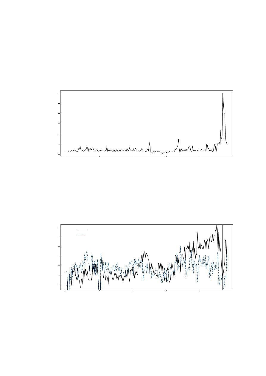
Figure 1: Interest Rates

Note: Annualized daily yields. The last transaction of day.

Day

100

100

150

200

200

300

400

500

600

50

0

0

Figure 2: Daily Lend and Borrow Order Flow,

b, l,

Note: In units of quadrillion, (qn.or 10

15

) Turkish liras (TRL).

Day

100

150

200

50

0

0.6

0

.8

1.0

1

.2

1.4

1

.6

1.8

234

l
b

32

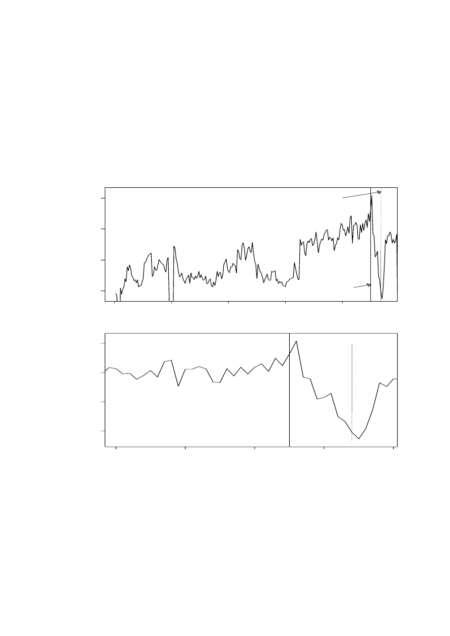
Figure 3: Daily Trading Volume in qn. TRL.

Note: In units of quadrillion, (qn.or 10

15

) Turkish liras (TRL).

100

150

200

50

0

1.5

2.0

2

.5

3.0

crisis period

Crisis day

Start of

(a) The Whole Sampling Period

200

225

220

230

240

210

1.5

2.0

2

.5

3.0

Stable period

Crisis period

Crisis day

234

(b) Days 200–240

33

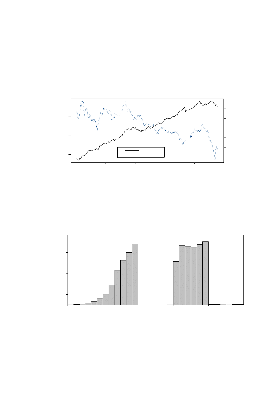
Figure 4: USD Exchange Rates and the Stock Market

Note: ISE (Istanbul Stock Exchange) is the main stock market index. USD is the exchange
rate of TRL/USD

ISE

ISE

USD

USD

Day

100

150

200

8,000

12,000

16,000

20,000

50

0

550,000

600,000

650,000

Figure 5: Intra Day Seasonality

Note: Average number of trades in each 10 minute interval.

n

u

m

b

er

of

trades

hour

100

10

11

12

13

14

60

20

30

80

0

120

34

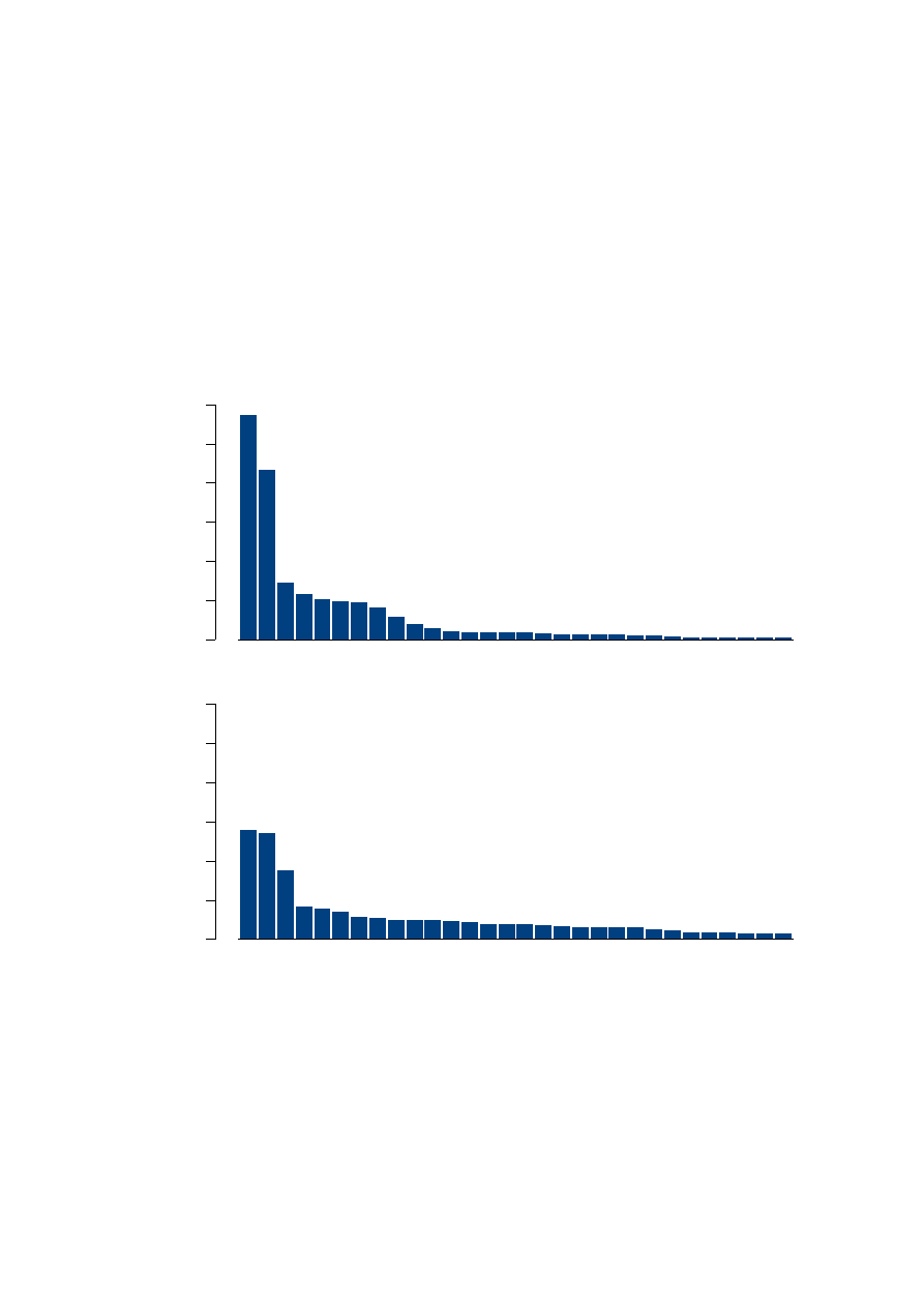
Figure 6: The Relative Trading Volume Of The 30 Largest Institutions

Note: In some cases the same institution might appear both as a borrowing and lending

institution.

0%

5%

15%

25%

10%

20%

30%

(a) Borrowers

0%

5%

15%

25%

10%

20%

30%

(b) Lenders

35