
Lecture Notes in Mathematics
1844
Editors:
J.--M. Morel, Cachan
F. Takens, Groningen
B. Teissier, Paris

3
Berlin
Heidelberg
New York
Hong Kong
London
Milan
Paris
Tokyo

Karl Friedrich Siburg
The Principle of Least Action in
Geometry and Dynamics
1 3

Author
Karl Friedrich Siburg
Fakult¨at f¨ur Mathematik
Ruhr-Universit¨at Bochum
44780 Bochum, Germany
e-mail: siburg@math.ruhr-uni-bochum.de
Library of Congress Control Number:
2004104313
Mathematics Subject Classification (2000): 37J , 53D, 58E
ISSN
0075-8434
ISBN
3-540-21944-7 Springer-Verlag Berlin Heidelberg New York
This work is subject to copyright. All rights are reserved, whether the whole or part of the material is
concerned, specif ically the rights of translation, reprinting, reuse of illustrations, recitation, broadcasting,
reproduction on microf ilm or in any other way, and storage in data banks. Duplication of this publication
or parts thereof is permitted only under the provisions of the German Copyright Law of September
9, 1965,
in its current version, and permission for use must always be obtained from Springer-Verlag. Violations are
liable for prosecution under the German Copyright Law.
Springer-Verlag Berlin Heidelberg New York a member of BertelsmannSpringer
Science + Business Media GmbH
http://www.springer.de
c
Springer-Verlag Berlin Heidelberg
2004
Printed in Germany
The use of general descriptive names, registered names, trademarks, etc. in this publication does not imply,
even in the absence of a specif ic statement, that such names are exempt from the relevant protective laws
and regulations and therefore free for general use.
Typesetting: Camera-ready TEX output by the author
SPIN:
11002192
41/3142/du-543210 - Printed on acid-free paper

Preface
The motion of classical mechanical systems is determined by Hamilton’s dif-
ferential equations:
˙x(t) = ∂
y
H(x(t), y(t))
˙
y(t) =
−∂
x
H(x(t), y(t))
For instance, if we consider the motion of n particles in a potential field, the
Hamiltonian function
H =
1
2
n
i=1
y
2
i
− V (x
1
, . . . , x
n
)
is the sum of kinetic and potential energy; this is just another formulation of
Newton’s Second Law.
A distinguished class of Hamiltonians on a cotangent bundle T
∗
X con-
sists of those satisfying the Legendre condition. These Hamiltonians are ob-
tained from Lagrangian systems on the configuration space X, with coordi-
nates (x, ˙
x) = (space, velocity), by introducing the new coordinates (x, y) =
(space, momentum) on its phase space T
∗
X. Analytically, the Legendre con-
dition corresponds to the convexity of H with respect to the fiber variable y.
The Hamiltonian gives the energy value along a solution (which is preserved
for time–independent systems) whereas the Lagrangian describes the action.
Hamilton’s equations are equivalent to the Euler–Lagrange equations for the
Lagrangian:
d
dt
∂
˙x
L(x(t), ˙
x(t)) = ∂
x
L(x(t), ˙
x(t)).
These equations express the variational character of solutions of the La-
grangian system. A curve x : [t
0
, t
1
]
→ R
n
is a Euler–Lagrange trajectory
if, and only if, the first variation of the action integral, with end points held
fixed, vanishes:
δ
t
1
t
0
L(x(t), ˙
x(t)) dt
x(t
1
)
x(t
0
)
= 0.

VI
Preface
In other words, solutions extremize the action with fixed end points on each
finite time interval.
This is not quite what one usually remembers from school
1
, namely that
solutions should minimize the action. The crucial point here is that the min-
imizing property holds only for short times. For instance, when looking at
geodesics on the round sphere, the movement along a great circle ceases to be
the shortest connection as soon as one comes across the antipodal point.
However, under certain circumstances there may well be action minimizing
trajectories. The investigation of these minimal objects is one of the central
topics of the present work. In fact, they do not always exist as genuine solu-
tions, but they do so as invariant measures. This is the outcome of a theory by
Mather and Ma˜
n´
e which generalizes Aubry–Mather theory from one to more
degrees of freedom. In particular, there exist action minimizing measures with
any prescribed “asymptotic direction” (described by a homological rotation
vector). Associating to each such rotation vector the action of a minimal mea-
sure, we obtain the minimal action functional
α : H
1
(X,
R) → R.
By construction, the minimal action does not describe the full dynamics but
concentrates on a very special part of it. The fundamental question is how
much information about the original system is contained in the minimal ac-
tion?
The first two chapters of this book provide the necessary background on
Aubry–Mather and Mather–Ma˜
n´
e theories. In the following chapters, we in-
vestigate the minimal action in four different settings:
1. convex billiards
2. fixed points and invariant tori
3. Hofer’s geometry
4. symplectic geometry.
We will see that the minimal action plays an important role in all four situa-
tions, underlining the significance of that particular variational principle.
1. Convex billards. Can one hear the shape of a drum? This was Kac’ pointed
formulation of the inverse spectral problem: is a manifold uniquely determined
by its Laplace spectrum? We do know now that this is not true in full gen-
erality; for the class of smooth convex domains in the plane, however, this
problem is still open.
We ask a somewhat weaker question for the length spectrum (i.e., the set
of lengths of closed geodesics) rather than the Laplace spectrum, which is
closely related to the previous one: how much geometry of a convex domain
is determined by its length spectrum? The crucial observation is that one can
consider this geometric problem from a more dynamical viewpoint. Namely,
1
depending on the school, of course. . .

Preface
VII
following a geodesic inside a convex domain that gets reflected at the bound-
ary, is equivalent to iterating the so–called billiard ball map. The latter is a
monotone twist map for which the minimal action is defined.
The main results from Chapter 3 can be summarized as follows.
Theorem 1. For planar convex domains, the minimal action is invariant un-
der continuous deformations of the domain that preserve the length spectrum.
In particular, every geometric quantity that can be written in terms of the
minimal action is automatically a length spectrum invariant.
In fact, the minimal action is a complete invariant and puts all previously
known ones (e.g., those constructed in [2, 19, 63, 87]) into a common frame-
work.
2. Fixed points and invariant tori. We consider a symplectic diffeomorphism
in a neighbourhood of an elliptic fixed point in
R
2
. If the fixed point is of
“general” type, the symplectic character of the map makes it possible (under
certain restrictions) to find new symplectic coordinates in which the map
takes a particularly simple form, the so–called Birkhoff normal form. The
coefficients of this normal form, called Birkhoff invariants, are symplectically
invariant.
The Birkhoff normal form describes an asymptotic approximation, in the
sense that it coincides with the original map only up to a term that vanishes
asymptotically when one approaches the fixed point. In general, it does not
give any information about the dynamics away from the fixed point.
The main result in this context introduces the minimal action as a sym-
plectically invariant function that contains the Birkhoff normal form, but also
reflects part of the dynamics near the fixed point.
Theorem 2. Associated to an area–preserving map near a general elliptic
fixed point there is the minimal action α, which is symplectically invariant.
It is a local invariant, i.e., it contains information about the dynamics
near the fixed point. Moreover, the Taylor coefficients of the convex conjugate
α
∗
are the Birkhoff invariants.
Area–preserving maps near a fixed point occur as Poincar´
e maps of closed
characteristics of three–dimensional contact flows. A particular example is
given by the geodesic flow on a two–dimensional Riemannian manifold. In
this case, the minimal action is determined by the length spectrum of the
surface, and we obtain the following result.
Theorem 3. Associated to a general elliptic closed geodesic on a two–dimen-
sional Riemannian manifold there is the germ of the minimal action, which is
a length spectrum invariant under continuous deformations of the Riemannian
metric.
The minimal action carries information about the geodesic flow near the
closed geodesic; in particular, it determines its C
0
–integrability.

VIII
Preface
In higher dimensions, we consider a symplectic diffeomorphism φ in a
neighbourhood of an invariant torus Λ. If we assume that the dynamics on Λ
satisfy a certain non–resonance condition, one can transform φ into Birkhoff
normal form again. If this normal form is positive definite the map φ deter-
mines the germ of the minimal action α, and we will show again that the
minimal action contains the Birkhoff invariants as Taylor coefficients of α
∗
.
3. Hofer’s geometry. Whereas the first three settings had many features in
common, the viewpoint here is quite different. Instead of looking at a single
Hamiltonian system, we investigate all Hamiltonian systems on a symplectic
manifold (M, ω) at once, collected in the Hamiltonian diffeomorphism group
Ham(M, ω). It is one of the cornerstones of symplectic topology that this group
carries a bi–invariant Finsler metric d, usually called Hofer metric, which is
constructed as follows.
Think of Ham(M, ω) as infinite–dimensional Lie group whose Lie algebra
consists of all smooth, compactly supported functions H : M
→ R with mean
value zero. Introduce any norm
· on those functions that is invariant under
the adjoint action H
→ H ◦ψ
−1
. Then the Hofer distance of a diffeomorphism
φ from the identity is defined as the infimum of the lengths of all paths in
Ham(M, ω) that connect φ to the identity:
d(id, φ) = inf
1
0
H
t
dt | ϕ
1
H
= φ
.
The problem is to choose the norm
·. The Hamiltonian system is determined
by the first derivatives of H, but
dH
C
0
, for instance, is not invariant under
the adjoint action. It turns out that the oscillation norm
· = osc := max − min
is the right choice although it seems to have nothing to do with the dynamics.
Loosely speaking, the Hofer metric generates a C
−1
–topology and measures
how much energy is needed to generate a given map.
The resulting geometry is far from being understood completely. This is
due to the fact that, despite its simple definition, the Hofer distance is very
hard to compute. After all, one has to take all Hamiltonians into account
that generate the same time–1–map. A fundamental question concerns the re-
lation between the Hofer geometry and dynamical properties of a Hamiltonian
diffeomorphism: does the dynamical behaviour influence the Hofer geometry
and, vice versa, can one infer knowledge about the dynamics from Hofer’s
geometry? Only little is known in this direction.
In Chap. 5, we take up this question for Hamiltonians on the cotan-
gent bundle T
∗
T
n
satisfying a Legendre condition. This leads to convex La-
grangians on T
T
n
for which the minimal action α is defined. On the other
hand, the Hamiltonians under consideration are unbounded and do not fit
into the framework of Hofer’s metric. Therefore, we have to restrict them to

Preface
IX
a compact part of T
∗
T
n
, e.g., to the unit ball cotangent bundle B
∗
T
n
, but in
such a way that we stay in the range of Mather’s theory.
Let α denote the minimal action associated to a convex Hamiltonian diffeo-
morphism on B
∗
T
n
. Our main result in this context shows that the oscillation
of α
∗
, which is nothing but α(0), is a lower bound for the Hofer distance. This
establishes a link between Hofer’s geometry of convex Hamiltonian mappings
and their dynamical behaviour.
Theorem 4. If φ
∈ Ham(B
∗
T
n
) is generated by a convex Hamiltonian then
d(id, φ)
≥ osc α
∗
= α(0).
4. Symplectic geometry. Consider the cotangent bundle T
∗
T
n
with its canon-
ical symplectic form ω
0
= dλ. Here, λ is the Liouville 1–form which is y dx in
local coordinates (x, y). Suppose H : T
∗
T
n
→ R is a convex Hamiltonian. Be-
cause H is time–independent the energy is preserved under the corresponding
flow, i.e., all trajectories lie on (fiberwise) convex (2n
−1)–dimensional hyper-
surfaces Σ =
{H = const.}. Of particular importance in classical mechanics
are so–called KAM–tori. i.e., invariant tori carrying quasiperiodic motion.
These are graphs over the base manifold
T
n
, with the additional property
that the symplectic form ω
0
vanishes on them; submanifolds with the latter
property are called Lagrangian submanifolds.
We want to study symplectic properties of Lagrangian submanifolds on
convex hypersurfaces. To do so, we observe that a Lagrangian submanifold
possesses a Liouville class a
Λ
, induced by the pull-back of the Liouville form
λ to Λ. The Liouville class is invariant under Hamiltonian diffeomorphisms,
i.e., it belongs to the realm of symplectic geometry. On the other hand, be-
ing a graph is certainly not a symplectic property. Our starting question in
this context is as follows: is it possible to move a Lagrangian submanifold Λ
on some convex hypersurface Σ by a Hamiltonian diffeomorphism inside the
domain U
Σ
bounded by Σ?
In a first part, we will see that, under certain conditions on the dynamics
on Λ, it is impossible to move Λ at all; we call this phenomenon boundary
rigidity. In fact, the Liouville class a
Λ
already determines Λ uniquely.
Theorem 5. Let Λ be a Lagrangian submanifold with conservative dynamics
that is contained in a convex hypersurface Σ, and let K be another Lagrangian
submanifold inside U
Σ
. Then
a
Λ
= a
K
⇐⇒ Λ = K.
What can happen if boundary rigidity fails? Surprisingly, even if it is pos-
sible to push Λ partly inside the domain U
Σ
, it cannot be done completely.
Certain pieces of Λ have to stay put, and we call them non–removable inter-
sections. In the case where Σ is some distinguished “critical” level set, these
non–removable intersections always contain an invariant subset with specific

X
Preface
dynamical behaviour; this subset is the so–called Aubry set from Mather–
Ma˜
n´
e theory. This result reveals a hidden link between aspects of symplectic
geometry and Mather–Ma˜
n´
e theory in modern dynamical systems.
Finally, we come back to the somewhat annoying fact that the property
of being a Lagrangian section is not preserved under Hamiltonian diffeomor-
phisms. For this, we consider
Theorem 6. Let U be a (fiberwise) convex subset U of T
∗
T
n
. Then every
cohomology class that can be represented as the Liouville class of some La-
grangian submanifold in U , can actually be represented by a Lagrangian sec-
tion contained in U .
So, from this rather vague point of view at least, Lagrangian sections actually
do belong to symplectic geometry.
Furthermore, the above result allows symplectic descriptions of seemingly
non–symplectic objects: the stable norm from geometric measure theory, and
also our favourite, the minimal action.
Theorem 7. The stable norm of a Riemannian metric g on
T
n
, and the min-
imal action of a convex Lagrangian L : T
T
n
→ R, both admit a symplectically
invariant description.
This closes the circle for our investigation of the Principle of Least Action
in geometry and dynamics.
Acknowledgement
: On behalf of the many people who supported and
encouraged me, I cordially thank Leonid Polterovich from Tel Aviv University
and Gerhard Knieper from the Ruhr–Universit¨
at Bochum.
This book was written while I was a Heisenberg Research Fellow. I am
grateful to the Deutsche Forschungsgemeinschaft for its generous support.

Contents
1
Aubry–Mather theory . . . . . . . . . . . . . . . . . . . . . . . . . . . . . . . . . . . . .
1
1.1
Monotone twist mappings . . . . . . . . . . . . . . . . . . . . . . . . . . . . . . . .
1
1.2
Minimal orbits . . . . . . . . . . . . . . . . . . . . . . . . . . . . . . . . . . . . . . . . . .
6
1.3
The minimal action for monotone twist mappings . . . . . . . . . . . .
8
2
Mather–Ma˜
n´
e theory . . . . . . . . . . . . . . . . . . . . . . . . . . . . . . . . . . . . . . 15
2.1
Mather’s minimal action . . . . . . . . . . . . . . . . . . . . . . . . . . . . . . . . . 15
2.1.1
The minimal action for convex Lagrangians . . . . . . . . . . . 16
2.1.2
A bit of symplectic geometry . . . . . . . . . . . . . . . . . . . . . . . 21
2.1.3
Invariant tori and the minimal action . . . . . . . . . . . . . . . . 23
2.2
Ma˜
n´
e’s critical value . . . . . . . . . . . . . . . . . . . . . . . . . . . . . . . . . . . . . 26
2.2.1
The critical value for convex Lagrangians . . . . . . . . . . . . . 26
2.2.2
Weak KAM solutions . . . . . . . . . . . . . . . . . . . . . . . . . . . . . . 29
2.2.3
The Aubry set . . . . . . . . . . . . . . . . . . . . . . . . . . . . . . . . . . . . 32
3
The minimal action and convex billiards . . . . . . . . . . . . . . . . . . . 37
3.1
Convex billiards . . . . . . . . . . . . . . . . . . . . . . . . . . . . . . . . . . . . . . . . . 38
3.2
Length spectrum invariants . . . . . . . . . . . . . . . . . . . . . . . . . . . . . . . 45
3.2.1
Classical invariants . . . . . . . . . . . . . . . . . . . . . . . . . . . . . . . . 49
3.2.2
The Marvizi–Melrose invariants . . . . . . . . . . . . . . . . . . . . . 52
3.2.3
The Gutkin–Katok width . . . . . . . . . . . . . . . . . . . . . . . . . . . 55
3.3
Laplace spectrum invariants . . . . . . . . . . . . . . . . . . . . . . . . . . . . . . 56
4
The minimal action near fixed points and invariant tori . . . . 59
4.1
The minimal action near plane elliptic fixed points . . . . . . . . . . . 60
4.2
Contact flows in three dimensions . . . . . . . . . . . . . . . . . . . . . . . . . 68
4.2.1
Spectral invariants . . . . . . . . . . . . . . . . . . . . . . . . . . . . . . . . . 71
4.2.2
Length spectrum invariants of surfaces . . . . . . . . . . . . . . . 74
4.3
The minimal action near positive definite invariant tori . . . . . . . 76

XII
Contents
5
The minimal action and Hofer’s geometry . . . . . . . . . . . . . . . . . 81
5.1
Hofer’s geometry of Ham(M, ω) . . . . . . . . . . . . . . . . . . . . . . . . . . . 82
5.2
Estimates via the minimal action . . . . . . . . . . . . . . . . . . . . . . . . . . 89
6
The minimal action and symplectic geometry . . . . . . . . . . . . . . 97
6.1
Boundary rigidity in convex hypersurfaces . . . . . . . . . . . . . . . . . . 98
6.1.1
Graph selectors for Lagrangian submanifolds . . . . . . . . . . 98
6.1.2
Boundary rigidity . . . . . . . . . . . . . . . . . . . . . . . . . . . . . . . . . 102
6.2
Non–removable intersections . . . . . . . . . . . . . . . . . . . . . . . . . . . . . . 105
6.2.1
Mather–Ma˜
n´
e theory for minimizing hypersurfaces . . . . . 105
6.2.2
The Aubry set and non–removable intersections . . . . . . . 110
6.3
Symplectic shapes and the minimal action . . . . . . . . . . . . . . . . . . 114
6.3.1
Lagrangian sections in convex domains . . . . . . . . . . . . . . . 115
6.3.2
Symplectic descriptions of the stable norm and the
minimal action . . . . . . . . . . . . . . . . . . . . . . . . . . . . . . . . . . . . 117
References . . . . . . . . . . . . . . . . . . . . . . . . . . . . . . . . . . . . . . . . . . . . . . . . . . . . . 121
Index . . . . . . . . . . . . . . . . . . . . . . . . . . . . . . . . . . . . . . . . . . . . . . . . . . . . . . . . . . 127

1
Aubry–Mather theory
The Principle of Least Action states that, for sufficiently short times, tra-
jectories of a Lagrangian system minimize the action amongst all paths in
configuration space with the same end points. If the time interval becomes
larger, however, the Euler–Lagrange equations describe just critical points of
the action functional; they may well be saddle points.
In the eighties, Aubry [5] and Mather [64] discovered independently that
monotone twist maps on an annulus possess orbits of any given rotation num-
ber which minimize the (discrete) action with fixed end points on all time
intervals. Roughly speaking, the rotation number of a geodesic describes the
direction in which the geodesic, lifted to the universal cover, travels. Those
minimal orbits turned out to be of crucial importance for a deeper under-
standing of the complicated orbit structure of monotone twist mappings.
Later, Mather [69] developed a similar theory for Lagrangian systems in
higher dimensions. There was, however, an old example by Hedlund [41] of
a Riemannian metric on
T
3
, having only three directions for which minimal
geodesics existed. Therefore, Mather’s generalization deals with minimal in-
variant measures instead of minimal orbits.
A different approach was suggested by Ma˜
n´
e [62] who introduced a certain
critical energy value at which the dynamics of a Lagrangian systems change.
It turned out that this approach essentially contains Mather’s theory, but in
a more both geometrical and dynamical setting.
We will deal with these generalizations of Aubry–Mather theory to higher
dimensions in Chap. 2.
1.1 Monotone twist mappings
Let
S
1
× (a, b) ⊂ S
1
× R = T
∗
S
1
be a plane annulus with
S
1
=
R/Z, where we allow the cases a = −∞ or
b = +
∞ (or both). Given a diffeomorphism φ of S
1
×(a, b) we consider a lift
φ
K.F. Siburg: LNM 1844, pp. 1–13, 2004.
c
Springer-Verlag Berlin Heidelberg 2004

2
1 Aubry–Mather theory
of φ to the universal cover
R × (a, b) of S
1
× (a, b) with coordinates x, y. Since
φ is a diffeomorphism, so is
φ, and we have
φ(x + 1, y) =
φ(x, y) + (1, 0). In
this section, we will always work with (fixed) lifts for which we drop the tilde
again and keep the notation φ.
In the case when a or b is finite we assume that φ extends continuously to
R × [a, b] by rotations by some fixed angles:
φ(x, a) = (x + ω
−
, a)
and
φ(x, b) = (x + ω
+
, b).
(1.1)
The numbers ω
±
are unique after we have fixed the lift. For simplicity, we set
ω
±
=
±∞ if a = −∞ or b = ∞.
Definition 1.1.1. A monotone twist map is a C
1
–diffeomorphism
φ :
R × (a, b) → R × (a, b)
(x
0
, y
0
)
→ (x
1
, y
1
)
satisfying φ(x
0
+ 1, y
0
) = φ(x
0
, y
0
) + (1, 0) as well as the following conditions:
1. φ preserves orientation and the boundaries of
R × (a, b), in the sense that
y
1
(x
0
, y
0
)
→ a, b as y
0
→ a, b;
2. if a or b is finite φ extends to the boundary by a rotation, i.e., it satisfies
(1.1);
3. φ satisfies a monotone twist condition
∂x
1
∂y
0
> 0;
(1.2)
4. φ is exact symplectic; in other words, there is a C
2
–function h, called a
generating function for φ, such that
y
1
dx
1
− y
0
dx
0
= dh(x
0
, x
1
).
(1.3)
The interval (ω
−
, ω
+
)
⊂ R, which can be infinite, is called the twist interval
of φ.
Remark 1.1.2. The twist condition (1.2) states that images of verticals are
graphs over the x–axis; see Fig. 1.1. This implies that φ can be described
in the coordinates x
0
, x
1
rather than x
0
, y
0
. In other words, for every choice
of x–coordinates x
0
and x
1
(corresponding to the configuration space), there
are unique choices y
0
and y
1
for the y–coordinates (corresponding to the
velocities) such that the image of (x
0
, y
0
) under φ is (x
1
, y
1
).
Remark 1.1.3. A generating function h for a twist map φ is defined on the
strip
{(ξ, η) ∈ R
2
| ω
−
< η
− ξ < ω
+
}
1.1 Monotone twist mappings
3
f
x
y
Fig. 1.1. The twist condition
and can be extended continuously to its closure. It is unique up to additive
constants. Equation (1.3) is equivalent to the system
∂
1
h(x
0
, x
1
) =
−y
0
∂
2
h(x
0
, x
1
) = y
1
(1.4)
Here, the expression ∂
i
denotes the partial derivative of a function with respect
to the i–th variable. The equivalent of the twist condition (1.2) for a generating
function is
∂
1
∂
2
h < 0.
(1.5)
Finally, a generating function satisfies the periodicity condition h(ξ +1, η +
1) = h(ξ, η).
Monotone twist maps are not as artificial as they might seem. They ap-
pear in a variety of situations, often unexpected and detected only by clever
coordinate choices. In the following, we give a few examples. The reader my
consult
Example 1.1.4. The simplest example is what is called an integrable twist map
which, by definition, preserves the radial coordinate
1
. In this case, the prop-
erty of being area–preserving implies that an integrable twist map is of the
following form:
φ(x
0
, y
0
) = (x
0
+ f (y
0
), y
0
)
with f
> 0. Then the generating function (up to additive constants) is given
by
1
In the context of integrable Hamiltonian systems, this means that (
x, y) are al-
ready the angle–action–variables.
4
1 Aubry–Mather theory
h = h(x
1
− x
0
),
with h
= f
−1
; in other words, h is strictly convex.
Example 1.1.5. In some sense the “simplest” non–integrable monotone twist
map is the so–called standard map
φ : (x, y)
→
x + y +
k
2π
sin 2πx, y +
k
2π
sin 2πx
where k
≥ 0 is a parameter. This map has been the subject of extensive
analytical and numerical studies. Famous pictures illustrate the transition
from integrability (k = 0) to “chaos” (k
≈ 10).
Example 1.1.6. A particularly interesting class of monotone twist maps comes
from planar convex billiards; we will deal with convex billiards in Chap. 3.
The investigation of such systems goes back to Birkhoff [15] who introduced
them as model case for nonlinear dynamical systems; for a modern survey see
[101].
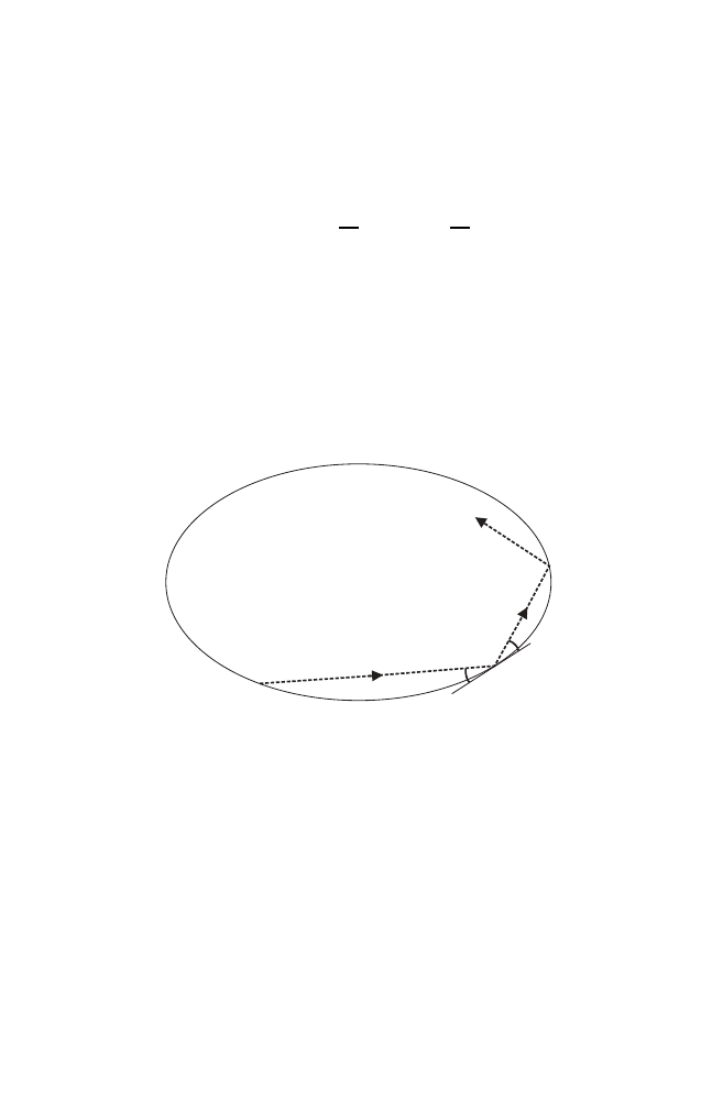
Fig. 1.2. The billard in a strictly convex domain
Given a strictly convex domain Ω in the Euclidean plane with smooth
boundary ∂Ω, we play the following game. Let a mass point move freely inside
Ω, starting at some initial point on the boundary with some initial direction
pointing into Ω. When the “billiard ball” hits the boundary, it gets reflected
according to the rule “angle of incidence = angle of reflection”; see Fig. 1.2.
The billiard map associates to a pair (point on the boundary, direction), re-
spectively (s, ψ) = (arclength parameter divided by total length, angle with
the tangent), the corresponding data when the points hits the boundary again.
The lift of this map, which is then defined on
R × (0, π), is not a monotone
twist map.
1.1 Monotone twist mappings
5
However, elementary geometry shows [101] that the map preserves the
2–form
sin ψ dψ
∧ ds = d(− cos ψ) ∧ ds.
Hence the billiard map preserves the standard area form dx
∧ dy in the new
coordinates
(x, y) = (s,
− cos ψ) ∈ R × (−1, 1).
Moreover, if you increase the angle with the positive tangent to ∂Ω for the
initial direction, the point where you hit ∂Ω again will move around ∂Ω in
positive direction. This means that
∂x
1
∂y
0
> 0,
so the billiard map in the new coordinates does satisfy the monotone twist
condition.
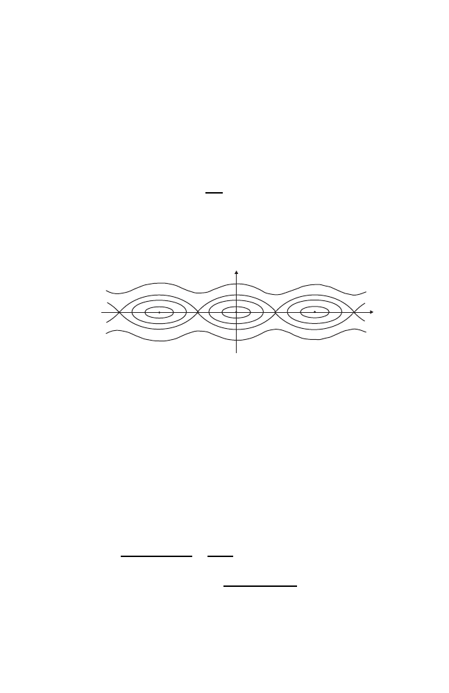
x
y
Fig. 1.3. The phase portrait of the mathematical pendulum
Example 1.1.7. Consider a particle moving in a periodic potential on the real
line. According to Newton’s Second Law, the motion of the particle is deter-
mined by the differential equation
¨
x(t) = V
(x(t)).
This can be written as a Hamiltonian system
˙x(t) = ∂
y
H(x(t), y(t))
˙
y(t) =
−∂
x
H(x(t), y(t))
with the Hamiltonian H(x, y) = y
2
/2
−V (x). For small enough t > 0, we have
∂x(t; x(0), y(0))
∂y(0)
=
∂
∂y(0)
t
0
˙
x(τ ; x(0), y(0)) dτ
=
t
0
∂y(τ ; x(0), y(0))
∂y(0)
dτ
> 0.

6
1 Aubry–Mather theory
Therefore the time–t–map ϕ
t
H
is a monotone twist map provided t is small.
In fact, this holds true not only for Hamiltonians of the form “kinetic energy
+ potential energy”, but for more general Hamiltonians which are fiberwise
convex in the second variable (corresponding to the momentum).
A particular case is that of a mathematical pendulum where x is the
angle to the vertical and V
(x) =
− sin 2πx. The phase portrait in R × R, see
Fig. 1.3, shows two types of invariant curves: closed circles around the stable
equilibrium (“librational” circles), and curves homotopic to the real line above
and below the separatrices (“rotational” curves).
Note that, by the monotone twist condition, an orbit ((x
i
, y
i
))
i
∈Z
of a
monotone twist map φ is completely determined by the sequence (x
i
)
i
∈Z
via
the relations
y
i
= ∂
2
h(x
i
−1
, x
i
) =
−∂
1
h(x
i
, x
i+1
).
Similarly, an arbitrary sequence (ξ
i
)
i
∈Z
corresponds to an orbit of a monotone
twist map φ if and only if
∂
2
h(ξ
i
−1
, ξ
i
) + ∂
1
h(ξ
i
, ξ
i+1
) = 0
(1.6)
for all i
∈ Z. Thus, on a formal level, orbits of a monotone twist mapping may
be regarded as “critical points” of the discrete action “functional”
(ξ
i
)
i
∈Z
→
i
∈Z
h(ξ
i
, ξ
i+1
)
on
R
Z
. This point of view leads to the following notion of minimal orbits.
1.2 Minimal orbits
Let φ : (x
0
, y
0
)
→ (x
1
, y
1
) be a monotone twist map with generating function
h(x
0
, x
1
). We have seen above that the φ–orbit of a point (x
0
, y
0
) is com-
pletely determined by the sequence (x
i
) of the first coordinates. Moreover, an
arbitrary sequence (ξ
i
) corresponds to an orbit if, and only if, it satisfies the
recursive relation (1.6). Loosely speaking, orbits are “critical points” of the
action “functional”
(ξ
i
)
i
∈Z
→
i
∈Z
h(ξ
i
, ξ
i+1
).
In this section, we are interested in minima, i.e. in points which minimize the
action.
This, of course, makes only sense if we restrict the action of a sequence
(ξ
i
)
i
∈Z
to finite parts. In analogy to the classical Principle of Least Action,
we define minimal orbits in such a way that they minimize the action with
the end points held fixed.

1.2 Minimal orbits
7
Definition 1.2.1. Let h be a generating function of a monotone twist map
φ. A sequence (x
i
)
i
∈Z
with ξ
i
∈ R is called minimal if every finite segment
minimizes the action with fixed end points, i.e., if
l
−1
i=k
h(x
i
, x
i+1
)
≤
l
−1
i=k
h(ξ
i
, ξ
i+1
)
for all finite segments (ξ
k
, . . . , ξ
l
)
∈ R
l
−k+1
with ξ
k
= x
k
and ξ
l
= x
l
.
By (1.6), each minimal sequence (x
i
)
i
∈Z
corresponds to a φ–orbit
((x
i
, y
i
))
i
∈Z
; these are called minimal orbits of φ.
Given an orbit (x
i
, y
i
) in
S
1
× (a, b), the twist map φ induces a circle
mapping on the first coordinates x
i
. This leads to the definition of the rotation
number of an orbit of a monotone twist map.
Definition 1.2.2. The rotation number of an orbit ((x
i
, y
i
))
i
∈Z
of a mono-
tone twist map is given by
ω := lim
|i|→∞
x
i
i
= lim
|i|→∞
x
i
− x
0
i
if this limit exists.
Example 1.2.3. The simplest orbits for which the rotation number always ex-
ists are periodic orbits, i.e., orbits ((x
i
, y
i
))
i
∈Z
with
x
i+q
= x
i
+ p
for all i
∈ Z, where p, q are integers with q > 0. In order to have q as the
minimal period one assumes that p and q are relatively prime. Then the
rotation number is given by
ω =
p
q
.
The questions arises whether there are orbits for a monotone twist map of
any given rotation number in the twist interval. Actually, this is the core of
Aubry–Mather theory, which yields an affirmative answer. The classical result
in this context is a theorem by G.D. Birkhoff [15] who proved that monotone
twist maps possess periodic orbits for each rational rotation number in their
twist interval. Perhaps because monotone twist maps were not that popular
in the mid-20th century, it took 60 years to generalize Birkhoff’s result to all
rotation numbers.
Theorem 1.2.4 (Birkhoff ). Let φ be a monotone twist map with twist in-
terval (ω
−
, ω
+
), and p/q
∈ (ω
−
, ω
+
) a rational number in lowest terms. Then
φ possesses at least two periodic orbits with rotation number p/q.

8
1 Aubry–Mather theory
Proof. The proof is a nice illustration of the use of variational methods in the
construction of specific orbits for monotone twist maps.
Consider the finite action functional
H(ξ
0
, . . . , ξ
q
) :=
q
−1
i=0
h(ξ
i
, ξ
i+1
)
on the set of all ordered (q + 1)–tuples with
ξ
0
≤ ξ
1
≤ . . . ≤ ξ
q
= ξ
0
+ p.
Since these tuples form a compact set, the continuous function H has a min-
imum, corresponding to a periodic orbit of the monotone twist map φ. What
we need to show is that this minimum does not lie on the boundary, which
consists of degenerate orbits of length less than q.
Suppose that there is a periodic orbit with
ξ
j
−1
< ξ
j
= ξ
j+1
< ξ
j+2
for some index j; the case of more than two equal values is treated analogously.
Then the recursive relation (1.6) yields
∂
2
h(ξ
j
−1
, ξ
j
) + ∂
1
h(ξ
j
, ξ
j+1
) = 0
∂
2
h(ξ
j
, ξ
j+1
) + ∂
1
h(ξ
j+1
, ξ
j+2
) = 0
Since ξ
j
= ξ
j+1
, substracting the two equations gives
∂
2
h(ξ
j
−1
, ξ
j
)
− ∂
2
h(ξ
j
, ξ
j
) + ∂
1
h(ξ
j+1
, ξ
j+1
)
− ∂
1
h(ξ
j+1
, ξ
j+2
) = 0.
This can be written as
∂
1
∂
2
h(η
1
, ξ
j
) (ξ
j
−1
− ξ
j
) + ∂
2
∂
1
h(ξ
j+1
, η
2
) (ξ
j+1
− ξ
j+2
) = 0,
where η
1
, η
2
are two intermediate values. But the left hand side is strictly
negative, due to (1.6) and the assumptions, which is a contradiction.
Birkhoff’s theorem is sharp in the sense that, in general, one cannot expect
more than two periodic orbits with a given rotation number. For example, in
the elliptical billiard, there are precisely two 2–periodic orbits, corresponding
to the two axes of symmetry.
1.3 The minimal action for monotone twist mappings
Of particular importance for the dynamics of a (projection of a) monotone
twist map φ :
S
1
× (a, b) → S
1
× (a, b) are closed invariant curves. They fall
into two classes: an invariant curve is either contractible or homotopically non-
trivial. Lifted to the strip
R × (a, b), this means that we consider φ–invariant
curves which are either closed or homotopic to
R.

1.3 The minimal action for monotone twist mappings
9
Definition 1.3.1. An invariant circle of a monotone twist map φ is an em-
bedded, homotopically nontrivial, φ–invariant curve in
S
1
×(a, b), respectively,
its lift to
R × (a, b).
Example 1.3.2. Considering the phase space
R × R of the mathematical pen-
dulum (see Fig. 1.3), the librational circles around the stable equilibria are
not invariant circles according to our definition. On the other hand, the rota-
tional curves above and below the separatrices do represent invariant circles.
Finally, the union of all the upper, respectively lower, separatrices also form
(non–smooth) invariant circles.
It turns out that invariant circles of monotone twists maps cannot take
any form. Indeed, another classical result by G.D. Birkhoff states that they
must project injectively onto the base. More precisely, we have the following
theorem.
Theorem 1.3.3 (Birkhoff ). Any invariant circle of a monotone twist map
is the graph of a Lipschitz function.
There are essentially two different proofs of this result. The original topo-
logical approach is indicated in [15,
§44] and [16, §3]; precise, and even more
general, proofs along this line can be found in [28, 42, 51, 66, 70]. The second
approach [94] is different and more dynamical. We give a sketch of its main
idea here and refer to [94] for details.
Proof ([94]). Assume, by contradiction, that there is an invariant circle Γ of
a monotone twist map φ which is not a graph. Then we have a situation like
that indicated in Fig. 1.4.
Let us apply φ once and see what happens to the area of the domain Ω
0
.
Since the preimage φ
−1
(v
1
) is a graph in view of the monotone twist condition,
and since φ is area–preserving, the application of φ pushes more area into the
fold, i.e., the area of Ω
1
is bigger than that of Ω
0
.
Now iterate φ, and consider the domains Ω
n
for n
≥ 1. Each application
lets the area of Ω
n
grow:
|Ω
n
| > |Ω
n
−1
| > . . . > |Ω
1
| > |Ω
0
|.
On the other hand, everything takes place in a bounded domain because Γ is
an invariant curve. Therefore, we conclude that sup
n
|Ω
n
| < ∞ which implies
the areas of the additional pieces tend to zero:
lim
n
→∞
|Ω
n
\ Ω
n
−1
| = 0.
But it is easy to see that this means that Γ must have a point of self–
intersection and, hence, is not embedded.
This contradiction proves the theorem.
10
1 Aubry–Mather theory
f
G
G
v
1
W
1
W
0
f
(v )
0
v
0
f
(v )
1
-1
Fig. 1.4. Applying a monotone twist map in a non–graph situation
Let us return to the question whether there are orbits of any given rotation
number for a monotone twist map. Theorem 1.2.4 asserts that there are always
periodic orbits for a given rational rotation number in the twist interval. By
taking limits of these orbits, one can construct also orbits of irrational rotation
numbers. All of these orbits are minimal.
Minimal orbits resemble invariant circles in the sense that they, too, project
injectively onto the base. In other words, minimal orbits lie on Lipschitz
graphs. Moreover, if there happens to be an invariant circle, then every orbit
on it is minimal.
The following theorem is the basic result in Aubry–Mather theory. The
reader may consult [6, 34, 51, 72, 74] for more details.
Theorem 1.3.4. A monotone twist map possesses minimal orbits for every
rotation number in its twist interval; for rational rotation numbers there are
always at least two periodic minimal orbits.
Every minimal orbit lies on a Lipschitz graph over the x–axis. Moreover,
if there exists an invariant circle then every orbit on that circle is minimal.
Remark 1.3.5. Theorem 1.3.4 remains true if one considers the more general
setting of a monotone twist map on an invariant annulus
{(x, y) | u
−
(x)
≤
y
≤ u
+
(x)
} between the graphs of two functions u
±
; see [72].
From the existence of orbits of any given rotation number, we can build a
function which will play a central role in our discussion. Namely, consider a
monotone twist with generating function h. Then we associate to each ω in
the twist interval the average h–action of some (and hence any) minimal orbit
((x
i
, y
i
))
i
∈Z
having that rotation number ω.

1.3 The minimal action for monotone twist mappings
11
Definition 1.3.6. Let φ be a monotone twist map with generating function h
and twist interval (ω
−
, ω
+
). Then the minimal action of φ is defined as the
function α : (ω
−
, ω
+
)
→ R with
α(ω) := lim
N
→∞
1
2N
N
−1
i=−N
h(x
i
, x
i+1
).
The minimal action can be seen as a “marked” Principle of Least Action:
it gives the (average) action of action–minimizing orbits, together with the
information to which topological type the corresponding minimal orbits be-
long. We wills see in Chap. 4 how this relates to the marked length spectrum
of a Riemannian manifold.
Does the minimal action tell us anything about the dynamics of the under-
lying twist map? This question is central from the dynamical systems point of
view. It turns out that, indeed, the minmal action does contain information
about the dynamical behaviour of the twist map.
The following theorem lists useful analytical properties of the minimal
action α.
Theorem 1.3.7. Let φ be a monotone twist map, and α its minimal action.
The the following holds true.
1. α is strictly convex; in particular, it is continuous.
2. α is differentiable at all irrational numbers.
3. If ω = p/q is rational, α is differentiable at p/q if and only if there is an
φ–invariant circle of rotation number p/q consisting entirely of periodic
minimal orbits.
4. If Γ
ω
is an φ–invariant circle of rotation number ω then α is differentiable
at ω with α
(ω) =
Γ
ω
y dx.
Proof. Everything is well known and can be found in [72, 68], except perhaps
for the precise value of α
(ω) in the last part. This follows from the more
general Thm. 2.1.24 and Rem. 2.1.7 in the next section.
For later purposes, we need a certain continuity property of the minimal
action as a functional. Namely, what happens with the minimal action if we
perturb the monotone twist map? It turns out that, at least for perturbations
of integrable twist maps, the minimal action behaves continuously. This is
made precise in the next proposition.
Proposition 1.3.8. Let h
0
be a generating function for an integrable twist
map such that
h
0
(s) = c(s
− γ)
k
+
O((s − γ)
k+1
)
as s
→ γ with c > 0 and k ≥ 2. Let h be a generating function for another
(not necessarily integrable) twist map such that

12
1 Aubry–Mather theory
h(ξ, η) = h
0
(η
− ξ) + O((η − ξ − γ)
k+m
)
as η
− ξ → γ with 2m ∈ N \ {0}.
Then the corresponding minimal actions α
0
and α satisfy
α
0
(ω) = h
0
(ω),
as well as
α(ω) = α
0
(ω) +
O((ω − γ)
k+m
)
as ω
→ γ.
Proof. Let us first convince ourselves that α
0
= h
0
. This follows from the fact
that all orbits of rotation number ω lie on the invariant circle
S
1
×{(h
0
)
−1
(ω)
}
and have the same average action h
0
(ω). Hence the minimal action α
0
(ω) is
indeed h
0
(ω).
For the continuity of the minimal action with respect to the generat-
ing function, we will use a monotonicity argument which is standard in the
calculus of variations; compare also [8]. Let us consider the minimal action
α = lim
N
→∞
1/2N
N
−1
i=−N
h(x
i
, x
i+1
), where (x
i
) is h–minimal, i.e.,
h(x
i
, x
i+1
)
≤ h(ξ
i
, ξ
i+1
)
for all finite sequences (ξ
i
) with the same end points. Note that the action
of an arbitrary segment (not necessarily part of an orbit) is monotone in the
generating function: if h
1
≤ h
2
then
i
h
1
(ξ
i
, ξ
i+1
)
≤
i
h
2
(ξ
i
, ξ
i+1
).
Moreover, the minimality of a sequence (x
i
) is defined by a minimization
process over all sequences (ξ
i
), a set which does not depend on the generating
function h. Hence, not just the action, but also the minimal action is monotone
in the generating function.
The monotonicity of the minimal action implies the second assertion.
Later, we will apply this proposition when γ = ω
−
is the lower boundary
point of the twist interval. Note that in this case we may have k = 3, for
instance, which would be forbidden if γ were a point in the twist interval
because then h
0
would not fulfill the generating function condition ∂
1
∂
2
h
0
=
−h
0
< 0.
Finally, since α is a convex function by Thm. 1.3.7, it possesses a convex
conjugate (or Fenchel transform) α
∗
defined by
α
∗
(I) := sup
ω
(ωI
− α(ω)).
(1.7)
Actually, α is strictly convex, so the supremum is a maximum, and α
∗
is a
convex, real-valued C
1
–function with

1.3 The minimal action for monotone twist mappings
13
(α
∗
)
(α
(ω)) = ω
whenever α
(ω) exists [90, Thm. 11.13]. Flat parts of α
∗
correspond to points
of non–differentiability of α.
2
2
See [90] for any question about smooth or non–smooth convex analysis.

2
Mather–Ma˜
n´
e theory
It was well known that the theory of Aubry and Mather concerning action–
minimizing orbits is valid only in two dimensions. For, there is a classical
example by Hedlund [41] of a Riemannian metric on
T
3
such that minimal
geodesics exist only in three directions. Hedlund’s construction modifies the
flat metric on
T
3
in such a way that there are three directions, corresponding
to three disjoint “highway tunnels”, along which the metric is very small, so
that the particle can travel along these highways and gather almost no action.
Hedlund shows that any minimal geodesic changes between the tunnels only
finitely often. Therefore, the asymptotic directions of minimal geodesics are
confined to the three tunnel directions.
Hedlund’s example showed that any generalization of Aubry–Mather the-
ory to higher dimensions could not deal with minimal orbits. Instead, Mather
[69] developed a corresponding theory of action–minimizing invariant mea-
sures for positive definite Lagrangian systems. Later, Ma˜
n´
e [62] gave another
approach using a so-called critical value. This value singled out the energy
value at which certain dynamically relevant orbits appear. Essentially, these
are two sides of one coin.
In this section, we will give an introduction to the relevant notions and
results. For further details we refer to [21, 29, 72].
2.1 Mather’s minimal action
The setting for Mather’s generalization of the theory of minimal orbits to
higher dimensions are convex Lagrangian (or Hamiltonian) systems on the
tangent (or cotangent) bundle of a compact manifold; we will restrict ourselves
to the case of the n–dimensional torus
T
n
=
R
n
/
Z
n
.
K.F. Siburg: LNM 1844, pp. 15–35, 2004.
c
Springer-Verlag Berlin Heidelberg 2004
16
2 Mather–Ma˜
n´
e theory
2.1.1 The minimal action for convex Lagrangians
For the convenience of the reader, we present a quick review of the classical
Lagrangian calculus of variations; for details we refer to [29, 33]. We denote
by x, p the canonical coordinates on the tangent bundle T
T
n
=
T
n
× R
n
. Any
C
2
–function L :
S
1
× T T
n
→ R, the so-called Lagrangian, gives rise to the
Euler–Lagrange flow ϕ
L
on T
T
n
, defined as follows.
The action of a C
1
–curve γ : [a, b]
→ T
n
is defined as the integral
A(γ) :=
b
a
L(t, γ(t), ˙γ(t))dt.
Curves that extremize the action among all curves with the same end points
are characterized by the Euler–Lagrange equation
d
dt
∂L
∂p
(t, γ(t), ˙γ(t)) =
∂L
∂x
(t, γ(t), ˙γ(t))
(2.1)
for all t
∈ [a, b]. Equation (2.1) is equivalent to
∂
2
L
∂p
2
(t, γ(t), ˙γ(t)) ¨
γ(t) =
∂L
∂x
(t, γ(t), ˙γ(t))
−
∂
2
L
∂x∂p
(t, γ(t), ˙γ(t)) ˙γ(t).
(2.2)
If the Lagrangian satisfies the so-called Legendre condition
det
∂
2
L
∂p
2
= 0,
then one can solve (2.2) for ¨
γ and, therefore, define a time–dependent vector
field X
L
(t, x, p) = ((x, p), (p, X
π
L
(t, x, p)) on T
T
n
such that the solutions of
¨
γ(t) = X
π
L
(t, γ(t), ˙γ(t)) are precisely the curves satisfying the Euler–Lagrange
equation (2.1). The vector field X
L
is called the Euler–Lagrange vector field,
and its flow is called the Euler–Lagrange flow ϕ
L
. It turns out that ϕ
L
is C
1
,
even if L is only C
2
.
Definition 2.1.1. A convex Lagrangian is a C
2
–function
L :
S
1
× T T
n
→ R
such that the following conditions hold.
1. Restricted to every fiber
{t} × T
x
T
n
, L is strictly convex; this means that
L has fiberwise positive definite Hessian:
∂
2
L
∂p
2
> 0.

2.1 Mather’s minimal action
17
2. L has fiberwise superlinear growth (with respect to some, and hence any,
Riemannian metric on
T
n
); this means that
lim
|p|→∞
L(x, p)
|p|
=
∞
uniformly in x.
3. The Euler–Lagrange flow ϕ
L
is complete, i.e., its solutions exist for all
times.
Example 2.1.2. A prime example of a flow generated by a convex Lagrangian
is the geodesic flow on
T
n
with respect to some Riemannian metric, where one
considers the free motion of a particle on
T
n
. The Lagrangian is then given
by
L(x, p) =
1
2
|p|
2
x
.
If one adds a potential V on
T
n
, the Lagrangian changes to
L(x, p) =
1
2
|p|
2
x
− V (x).
Remark 2.1.3. A Lagrangian is by no means uniquely defined by the Euler–
Lagrange flow. Indeed, if L generates the flow ϕ
L
, then also the new La-
grangian
L(x, p)
− ν
x
(p),
where ν is any closed 1–form on
T
n
, generates the same ϕ
L
.
This can be seen as follows. The actions of a curve γ with respect to L
and L
− ν differ by the term
γ
ν. Since ν is closed, Stokes’ Theorem im-
plies that this term does not depend on the curve γ (in the same homotopy
class). Therefore the actions differ only by some additive constant, and so the
extremal curves are the same.
Note that for convex L, the new Lagrangian L
ν
is also convex.
Let L be a convex Lagrangian. In the following, we will not deal with
orbits of the Euler–Lagrange flow ϕ
L
, but rather with invariant probability
measures. To do so, we denote by
M
L
the set of ϕ
L
–invariant probability
measures on T
T
n
. For µ
∈ M
L
we call
A(µ) =
L dµ
∈ R ∪ {+∞}
its action. To each µ
∈ M
L
, one associates the linear functional
H
1
(
T
n
,
R) → R , [ν] →
ν dµ
where we view a 1-form ν as a function on T
T
n
that is linear on the fibers.
By duality, there is a unique class ρ(µ)
∈ H
1
(
T
n
,
R) such that

18
2 Mather–Ma˜
n´
e theory
ν dµ =
[ν], ρ(µ)
(2.3)
for all [ν]
∈ H
1
(
T
n
,
R).
Definition 2.1.4. Let µ
∈ M
L
be an invariant measure for a convex La-
grangian L. Then the class ρ(µ)
∈ H
1
(
T
n
,
R), defined by (2.3), is called the
rotation vector of µ.
Remark 2.1.5. The rotation vector of an invariant measure is related to
Schwartzman’s asymptotic cycles [91]; see [21].
In analogy to Aubry–Mather theory in two dimensions, we want to min-
imize the action of all invariant measures having the same rotation vector.
Although the tangent bundle of
T
n
is not compact, this can be dealt with
by taking its one point compactification, adding a point at infinity; see [69].
Then
M
L
becomes compact with respect to the vague (weak
∗
) topology [14],
and we actually can minimize the action over the set of invariant probability
measures having a given rotation vector.
Definition 2.1.6. Let L be a convex Lagrangian. Then the function
α : H
1
(
T
n
,
R) → R
h
→ min{A(µ) | µ ∈ M
L
, ρ(µ) = h
}
is called the minimal action of L.
Any invariant measure µ
∈ M
L
realizing this minimum, i.e. with A(µ) =
α(ρ(µ)), is called a minimal measure. For a fixed rotation vector h
∈ H
1
(
T
n
,
R),
the set of all minimal measures with ρ(µ) = h is denoted by
M
h
.
Remark 2.1.7. In the case of one degree of freedom (n = 1), the theory of
Mather–Ma˜
n´
e reproduces the discrete Aubry–Mather theory from Chap. 1.
To see this, one uses the result by Moser [78] that every monotone twist
map on the cylinder is the time–1–map of a convex Lagrangian; see also [93].
Then it is shown in [67] that the minimal action α(ρ(µ)) in the continuous
setting considered here is, perhaps after adding a constant, the same as the
minimal action α(ω) in the discrete framework of Aubry–Mather theory where
ρ(µ) = ω. Hence we need not distinguish between the two.
Remark 2.1.8. The relation between minimizing measures and globally mini-
mizing orbits is quite delicate, and we refer to [21] for details. We mentioned
Hedlund’s example [41] showing that minimal orbits for an arbitrary rotation
vector need not always exist. At least, every trajectory that lies in the union
of all supports of minimal measures in
M
h
minimizes the action among all
curves in the universal cover
R
n
with the same end points [69, Prop. 3]. The
dynamics on the set of minimizing trajectories is not limited to any particular
behaviour—it can be as complicated as that of any vector field on the base
manifold [60].

2.1 Mather’s minimal action
19
Let us consider the minimal action α. Recall from Thm. 1.3.7 that, in the
two-dimensional discrete setting of Aubry–Mather theory, the minimal action
is a strictly convex function. We want to prove a similar result for the higher
dimensional case.
Proposition 2.1.9. The minimal action α : H
1
(
T
n
,
R) → R is a convex,
superlinear function.
Proof. Let h
1
, h
2
∈ H
1
(
T
n
,
R) and λ ∈ [0, 1]. Choose minimal measures
µ
1
, µ
2
∈ M
L
such that ρ(µ
i
) = h
i
. Then the convex combination
µ := λµ
1
+ (1
− λ)µ
2
lies in
M
L
and has rotation vector ρ(µ) = λh
1
+ (1
− λ)h
2
. Since both µ
1
and
µ
2
are minimal, we conclude that
α(λh
1
+ (1
− λ)h
2
)
≤ A(µ) = λα(h
1
) + (1
− λ)α(h
2
),
which proves the convexity of α.
As for the superlinearity, we refer to [69] or [29][Thm. 4.4.5].
Remark 2.1.10. In contrast to the two–dimensional case, the function α need
not be strictly convex.
As a convex function, α possesses a convex conjugate
α
∗
: H
1
(
T
n
,
R) → R
(2.4)
c
→ sup
h
∈H
1
(
c, h − α(h))
(2.5)
Since α is superlinear, the supremum is a maximum and attained at h
c
∈
H
1
(
T
n
,
R) if, and only if,
α(h)
≥ α(h
c
) +
c, h − h
c
for all h, in other words, if c is a subgradient of α at h
c
; compare, for instance,
[90, 29]. We arrive at the following equivalent formulations for the minimality
of a measure µ:
• there exists a homology class h ∈ H
1
(
T
n
,
R), namely the rotation vector
ρ(µ), such that µ minimizes the action
L dµ amongst all measures in
M
L
with rotation vector h;
• there exists a cohomology class c = [ν] ∈ H
1
(
T
n
,
R), namely any subgra-
dient of α at ρ(µ), such that µ minimizes
L
− ν dµ amongst all measures
in
M
L
.
Note that L
− ν is again a convex Lagrangrian and generates the same flow
as L because ν is closed. Therefore,
M
L
−ν
=
M
L
; see Rem. 2.1.3.
Let us continue with the idea to prove results, analogous to those in Aubry–
Mather theory, in the more general setting of Mather’s theory of minimal

20
2 Mather–Ma˜
n´
e theory
measures. Recall that Thm. 1.3.4 stated that minimal orbits of monotone
twist maps always lie on Lipschitz graphs. Thus, one is lead to the conjecture
that the supports of minimal measures (corresponding to minimal orbits)
should lie on Lipschitz graphs over
T
n
(seen as the zero section in T
T
n
).
In fact, this conjecture is true. The following is Mather’s so-called Lipschitz
Graph Theorem from [69]; see also [21].
Theorem 2.1.11. For every h
∈ H
1
(
T
n
,
R), the union of the supports of all
minimal measures in
M
h
lies on a Lipschitz graph over
T
n
. Moreover, the
Lipschitz constant depends only on the Lagrangian L and not on the rotation
vector h.
Important dynamical objects for twist maps are invariant circles; in higher
dimensions, the corresponding objects are invariant tori. We know from
Thm. 1.3.4 that orbits on invariant circles are automatically minimal. What
is the corresponding result in higher dimensions? We point out that invariant
tori of convex Lagrangian systems are only shown to be graphs under cer-
tain assumptions on their dynamics; see [10] for a generalization of Birkhoff’s
Theorem 1.3.3 to higher dimensions.
In order to deal with invariant tori, it is convenient to reformulate every-
thing in the Hamiltonian, rather than in the Lagrangian, framework. Given a
convex Lagrangian L :
S
1
× T T
n
→ R, the so-called Legendre transformation
:
S
1
× T T
n
→ S
1
× T
∗
T
n
(t, x, p)
→ (t, x, y := ∂
p
L)
(2.6)
is a diffeomorphism between the tangent and the cotangent bundle. It yields
the convex Hamiltonian H :
S
1
× T
∗
T
n
→ R defined by
H(t, x, y) :=
y, p − L(t, x, p)|
p=(∂
p
L)
−1
(y)
.
The Hamiltonian H gives rise to the Hamiltonian flow ϕ
H
on the cotangent
bundle via the Hamiltonian equations, written in local coordinates as
˙
x(t) = ∂
y
H(t, x(t), y(t))
˙
y(t) =
−∂
x
H(t, x(t), y(t))
(2.7)
Then the Legendre transformation provides a conjugation between the Hamil-
tonian flow ϕ
H
on T
∗
T
n
and the Euler–Lagrange flow ϕ
L
on T
T
n
. We refer
to [33, 21] for more details.
Given a Hamiltonian flow ϕ
H
on T
∗
T
n
, we denote its time–t–map by
ϕ
t
H
: T
∗
T
n
→ T
∗
T
n
.
This yields a one–to–one correspondence between ϕ
L
–invariant probability
measures and ϕ
H
– or ϕ
1
H
–invariant ones. For simplicity, we do not introduce
three different notations but write µ for any of those. Likewise, we define the
minimal action associated to a convex Hamiltonian H to be that associated to
L and write α in either case. We say that a ϕ
H
– or ϕ
1
H
–invariant probability
measure is minimal if its ϕ
L
–invariant counterpart is.

2.1 Mather’s minimal action
21
2.1.2 A bit of symplectic geometry
The Hamiltonian viewpoint is the viewpoint of symplectic geometry. Let us
recall a few notions; see [73] for a comprehensive introduction to symplectic
geometry.
Definition 2.1.12. A symplectic form ω on a manifold M is a closed non-
degenerate 2–form. A symplectic manifold (M, ω) is a manifold M , equipped
with a symplectic form ω.
Example 2.1.13. The 2n–dimensional Euclidean space
R
2n
, together with the
so–called canonical symplectic form
ω
0
:= dy
∧ dx =
n
i=1
dy
i
∧ dx
i
,
is called the standard symplectic space. Note that the dimension of a symplectic
manifold must always be even in view of the nondegeneracy condition on the
2-form ω.
Example 2.1.14. An important example of a symplectic manifold is the cotan-
gent bundle T
∗
X of an n–dimensional manifold X. It carries a canonical
symplectic form ω = dλ that is not just closed but even exact. Here, the
1-form λ is the so–called Liouville form which, in local coordinates, is given
by
λ := y dx =
n
i=1
y
i
dx
i
.
This local definition admits a global interpretation as follows. Let
θ : T
∗
X
→ X
be the canonical projection, and ξ
∈ T
(x,y)
T
∗
X. Then
λ
(x,y)
(ξ) = (θ
∗
y
x
)(ξ).
Of particular interest in symplectic geometry are submanifolds Λ
⊂ M of
s symplectic manifold (M, ω) on which the symplectic form vanishes:
ω
|
T Λ
= 0.
Such submanifolds are called isotropic. It follows from the nondegeneracy of
ω that dim Λ
≤ 1/2 dim M for isotropic submanifolds Λ.
Definition 2.1.15. A Lagrangian submanifold Λ of a symplectic manifold
(M, ω) is an isotropic manifold of maximal dimension; in other words, we
have
dim Λ =
1
2
dim M
and
ω
|
T Λ
= 0.

22
2 Mather–Ma˜
n´
e theory
Example 2.1.16. In the standard symplectic space, the submanifold
{(x, y) ∈
R
2n
| y = 0} is a Lagrangian submanifold, whereas {(x, y) ∈ R
2n
| x = 0} is
not.
Example 2.1.17. Let ν be a 1–form on some manifold X. Then the graph
gr ν :=
{(x, ν
x
)
| x ∈ X}
is a Lagrangian submanifold of (T
∗
X, dλ) if, and only if, the 1–form ν is
closed. Such a Lagrangian manifold, which projects injectively onto the base,
is called a Lagrangian graph or Lagrangian section.
In our case where M = T
∗
T
n
, any Lagrangian submanifold that is diffeo-
morphic to
T
n
is called a Lagrangian torus. For instance, if n = 1, any circle
on the cylinder is a Lagrangian torus (or circle, rather).
We want to define Hamiltonian flows on symplectic manifolds. To do so,
let H :
S
1
× M → R be a time–periodic Hamiltonian on some symplectic
manifold (M, ω), and denote by H
t
: M
→ R the function for fixed t.
Definition 2.1.18. The Hamiltonian vector field X
H
on M associated to a
Hamiltonian H is defined by
i
X
H
ω =
−dH
t
,
where i
X
H
ω := ω(X
H
,
·) is the usual contraction of a form by a vector field.
Example 2.1.19. If (M, ω) = (
R
2n
, ω
0
) is the standard symplectic space then
the Hamiltonian vector field is given by
X
H
(x, y) = J
∇H
t
(x, y),
where J is the 2n
× 2n–matrix
J :=
0 1
−1 0
.
In other words, we arrive at our familiar system (2.7).
The invariance group of a symplectic manifold consists of all diffeomor-
phisms that leave the symplectic form invariant.
Definition 2.1.20. A map φ : M
→ M of a symplectic manifold (M, ω) is
called symplectic if it preserves the symplectic form ω:
φ
∗
ω = ω.
Example 2.1.21. Certainly, the identity is symplectic. More generally, every
time–t–map ϕ
t
H
of a Hamiltonian flow is symplectic since, by Cartan’s formula
for the Lie derivative, we have
d
dt
(ϕ
t
H
)
∗
ω = L
X
H
ω = di
X
H
ω + i
X
H
dω = d(
−dH
t
) = 0.

2.1 Mather’s minimal action
23
Example 2.1.22. On a cotangent bundle T
∗
X with coordinates (x, y) and
canonical symplectic form (see Ex. 2.1.14), we have the symplectic shift map-
ping
(x, y)
→ (x, y − ν)
where ν is some closed 1–form on X.
2.1.3 Invariant tori and the minimal action
Let us return to our original setting. We know from Thm. 1.3.4 that invariant
circles of monotone twist maps carry minimal orbits. In higher dimensions,
a similar statement is true. Namely, let φ = ϕ
1
H
be generated by a convex
Hamiltonian on
S
1
× T
∗
T
n
, and suppose that φ possesses an invariant La-
grangian torus Λ which is a graph. This situation occurs, for instance, in
KAM–theory where one considers small perturbations of convex, completely
integrable Hamiltonian systems.
Definition 2.1.23. Consider a cotangent bundle θ : T
∗
X
→ X with its
canonical symplectic form ω = dλ. We denote by
L the class of all Lagrangian
submanifolds of T
∗
X which are Lagrangian isotopic to the zero section
O.
Given Λ
∈ L, the natural projection θ|
Λ
: Λ
→ X induces an isomorphism
between the cohomology groups H
1
(X,
R) and H
1
(Λ,
R). The preimage a
Λ
∈
H
1
(X,
R) of [λ|
Λ
]
∈ H
1
(Λ,
R) under this isomorphism is called the Liouville
class of Λ.
The next theorem, firstly, says that Λ consists of supports of minimal
measures and, secondly, shows that the Liouville class of Λ is a subgradient of
the minimal action. Recall that a vector v
∈ R
n
is a subgradient of a function
f :
R
n
→ R at x ∈ R
n
if
f (y)
≥ f(x) + v, y − x
for all y
∈ R
n
. If we have a strict inequality for all y
= x, we say that v is a
subgradient with only one point of tangency. For instance, if f is differentiable
at x then, of course, its gradient
∇f(x) is its unique subgradient at x. See
[90] for more details.
Theorem 2.1.24. Let φ = ϕ
1
H
be generated by a convex Hamiltonian H on
S
1
× T
∗
T
n
. Suppose that φ possesses an invariant Lagrangian torus Λ in
(T
∗
T
n
, dλ) such that Λ is homologous to the zero section and φ
|
Λ
is conjugated
to a translation on
T
n
by some fixed vector ρ.
Then every φ–invariant probability measure with support in Λ is minimal,
and a
Λ
∈ H
1
(
T
n
,
R) is a subgradient of the minimal action α of H at ρ with
only one point of tangency. Vice versa, every minimal measure of rotation
vector ρ has support in Λ.

24
2 Mather–Ma˜
n´
e theory
We point out that an observation by Herman [43, Prop. 3.2] shows that
the condition on Λ being Lagrangian can be dropped if the vector (1, ρ) is
rationally independent, e.g. for invariant KAM–tori; in this case the minimal
measure supported on Λ is unique.
Proof. We proceed in three steps and reduce each to the previous one. First of
all, by a higher-dimensional version of Birkhoff’s Theorem [10] the tori ϕ
t
H
(Λ)
are graphs for all t
∈ [0, 1]; for our assumption on ϕ|
Λ
says, in particular, that
ϕ
|
Λ
preserves a measure which is positive on open sets (cf. [10, Prop. 1.2.(ii)]).
Note that, as a Lagrangian graph, ϕ
t
H
(Λ) is the graph of a closed 1-form ν
t
;
by invariance, ν
0
= ν
1
.
Case 1 : Our starting point is the simplest possible, where Λ =
O is the
zero section and remains invariant under the flow, i.e.
ν
t
= 0
for all t. Then
0 = y(t) = ∂
p
L(t, x(t), ˙
x(t))
and
0 =
d
dt
∂
p
L(t, x(t), ˙
x(t)) = ∂
x
L(t, x(t), ˙
x(t))
for all orbits starting (and hence lying) on
O. Note that
−1
O, the preimage
of
O under the Legendre transformation, will depend on t unless ˙x(t) = ρ for
all t.
In any case, we have
∇L
t
|
−1
O
= 0 which, by convexity of L, implies that
L
t
(x, p) = min L
t
⇐⇒ (x, p) ∈
−1
O.
Consequently, an invariant measure µ
∈ M
L
is globally minimizing if, and
only if, its support lies in
−1
O. Since all orbits in O have rotation vector ρ
we see that for any such µ we have
L dµ =
1
0
min L
t
dt = α(ρ).
In addition, α(h) > α(ρ) if h
= ρ, so 0 = a
O
is a subgradient of α at ρ with
only one point of tangency.
Case 2 : Next we consider the case when Λ is still the zero section but does
not stay invariant under the flow; more precisely, we assume that
ν
t
= dS
t
for some function S
t
on
T
n
with ν
0
= ν
1
. (S
t
is a generating function in the
simplest case where the Lagrangian ϕ
t
H
(
O) is a graph.)
We define the new Hamiltonian
K(t, x, y) = ∂
t
S
t
(x) + H(t, x, y + dS
t
(x)).

2.1 Mather’s minimal action
25
It is convex, and if we write ϕ
t
H
(x, y) = (x(t), y(t)) the transformation law of
Hamiltonian vector fields yields
ϕ
t
K
(x, y) = ϕ
t
∂
t
S
t
◦ ϕ
t
H
(x, y) = (x(t), y(t)
− dS
t
(x(t))).
Therefore, ϕ
1
K
= ϕ
1
H
= ϕ and ϕ
t
K
(x, 0) = (x(t), 0).
Now we are in the first case with H replaced by K. This changes the
(minimal) action only by an additive constant [67], and the same conclusions
hold as before.
Case 3 : In the general case, we apply the symplectic shift
(x, y)
→ (x, y − ν
0
).
This maps Λ onto the zero section
O and the 1–form λ onto λ = λ − λ|
Λ
; the
new flow ϕ
t
H
maps
O onto the graph of ν
t
= ν
t
− ν
0
. A generating function
for ϕ
t
H
is given by
S
t
(x) =
t
0
−
H(s, ϕ
s
H
◦ (ϕ
t
H
)
−1
(x, ν
t
(x))) ds.
Thus we are back in Case 2, but this time with with a different 1-form
λ
instead of λ. It is shown in [67] that the actions behave like
A(µ) = A(µ) +
[λ − λ], ρ(µ) = A(µ) − a
Λ
, ρ(µ)
.
From Case 2 we know that every µ with support in Λ minimizes
A(µ) among
all measures with ρ(µ) = ρ. But under this constraint the correction term
a
Λ
, ρ
is a mere constant, so µ minimizes A(µ), too. Moreover, 0 is a sub-
gradient of
α(h) = α(h) − a
Λ
, h
at ρ with only one point of tangency. That
means that
α(h)
≥ α(ρ) + a
Λ
, h
− ρ
with equality only for h = ρ, so a
Λ
is a subgradient of α at ρ with only one
point of tangency.
This finishes the proof of the theorem.
Corollary 2.1.25. If, under the assumptions of Theorem 2.1.24, the invari-
ant torus Λ is invariant under the flow of H (and not just its time–1–map)
then
α
∗
(a
Λ
) =
1
0
H(t,
·)|
Λ
dt.
Proof. Theorem 2.1.24 implies that α
∗
(a
Λ
) =
a
Λ
, ρ
− α(ρ) =
λ
|
Λ
− L dµ
for every invariant measure µ supported in Λ. Since Λ is invariant under the
Hamiltonian flow, the function H(t,
·) is constant on Λ with H = λ|
Λ
− L.
Remark 2.1.26. If H is autonomous, Corollary 2.1.25 determines the energy
level of invariant tori with given α
∗
(a
Λ
); compare [25].

26
2 Mather–Ma˜
n´
e theory
2.2 Ma˜
n´
e’s critical value
Another approach to a generalization of Aubry–Mather theory to higher di-
mensions was suggested by Ma˜
n´
e [62]. Its main idea is to single out a certain
energy level at which a significant change of the dynamical behaviour takes
place. This produces a “critical” energy value for each convex Lagrangian.
It turns out that this value is the minimum of the actions of all invariant
measures in
M
L
, and that one can recover Mather’s minimal action from it
(and vice versa).
2.2.1 The critical value for convex Lagrangians
Let L : T
T
n
→ R be a time-independent convex Lagrangian on the tangent
bundle of the n–torus. Let : T
T
n
→ T
∗
T
n
be the Legendre transformation,
and H : T
∗
T
n
→ R the Hamiltonian corresponding to L. The push–forward
of the Euler–Lagrange flow ϕ
L
on T
T
n
by the Legendre transformation is
the Hamiltonian flow ϕ
H
on T
∗
T
n
with respect to the canonical symplectic
structure on T
∗
T
n
; see Sect. 2.1.2. The energy of L is the function E : T
T
n
→
R defined by
E(x, p) :=
∂L
∂p
(x, p), p
− L(x, p) = H((x, p)).
It is a first integral of the Euler–Lagrange flow ϕ
L
.
Recall that a curve γ : [a, b]
→ T
n
is called absolutely continuous if for
every > 0 there exists δ > 0 so that for each finite collection of pair-
wise disjoint open intervals (s
i
, t
i
) in [a, b] of total length less than δ one has
i
dist(γ(t
i
), γ(s
i
)) < ; here dist is any Riemannian distance on
T
n
. As be-
fore, the action of an absolutely continuous curve γ : [a, b]
→ T
n
is defined
by
A
L
(γ) :=
b
a
L(γ(t), ˙γ(t)) dt.
We keep the subscript L in order to distinguish between the actions for dif-
ferent Lagrangians.
Given two points x
1
, x
2
∈ T
n
and some T > 0, denote by
C
T
(x
1
, x
2
) the set
of absolutely continuous curves γ : [0, T ]
→ T
n
with γ(0) = x
1
and γ(T ) = x
2
.
For each k
∈ R, we define
Φ
k
(x
1
, x
2
; T ) := inf
{A
L+k
(γ)
| γ ∈ C
T
(x
1
, x
2
)
}
as the infimum of the (L + k)–actions over all curves connecting x
1
and x
2
in
time T .
Definition 2.2.1. Let L : T
T
n
→ R be a convex Lagrangian. Then the action
potential Φ
k
:
T
n
× T
n
→ R ∪ {−∞} of L is defined as
2.2 Ma˜
n´
e’s critical value
27
Φ
k
:
T
n
× T
n
→ R ∪ {−∞}
(x
1
, x
2
)
→ inf
T >0
Φ
k
(x
1
, x
2
; T )
The critical value of L is given by
c(L) := inf
{k ∈ R | Φ
k
(x, x) >
−∞ for some x ∈ T
n
}.
x
y
go around
many times
g
g
Fig. 2.1. If A
L+k
(
γ) < 0 then Φ
k
(
x, y) = −∞
Remark 2.2.2. Observe that if there is some closed curve γ with A
L+k
(γ) < 0
then immediately Φ
k
(x, y) =
−∞ for all x, y. This follows by considering the
curve going from x to some point on γ, going around as many times as one
wishes (gathering as much negative action as one wants), and finally going to
y; see Fig. 2.1. Thus, we could replace the word “some” in the definition of
c(L) by “all”. Since the action potential is monotone in k, we then have
c(L) = sup
{k ∈ R | there is a closed curve γ with A
L+k
(γ) < 0
},
(2.8)
which gives another description of the critical value.
Remark 2.2.3. We will explain why c(L) is a real number. Think of some
Lagrangian, and pick a point x
∈ T
n
. Consider the infimum of the actions of
all closed curves through x. Since the time interval is free, you will get
−∞ for
the infimum as soon as you have just one closed curve with negative action.
Now let L be a fixed Lagrangian. We want to see what happens if we
shift L by some constant k. If k <
− min
x
L(x, 0) then L(x, 0) + k is negative
at some point x, we can choose the constant curve at x, and end up with
Φ
k
(x, x) =
−∞. On the other hand, the fact that L is convex implies that L
is bounded from below. Therefore, if k >
− min L then L + k is positive, and
we must have Φ
k
(x
1
, x
2
; T ) > 0 for all x
1
, x
2
, T . This shows that
c(L) <
∞
is a real number.

28
2 Mather–Ma˜
n´
e theory
The critical value can in fact be characterized in a variety of ways [60, 20,
22, 23]. Each of these characterizations gives new insight into the geometry
or the dynamics of the given Lagrangian system. In the following, we will
explain the relation between the critical value and the minimal action defined
in Sect. 2.1.
Let
M
L
be the set of invariant probability measures on T
T
n
. The next
result, due to Ma˜
n´
e [60], states that the critical value of a convex Lagrangian is
equal to the minmal action of all measures in
M
L
, regardless of their rotation
vector.
Proposition 2.2.4.
c(L) =
− min{A
L
(µ)
| µ ∈ M
L
}.
Proof. First of all, one can show that
min
{A
L
(µ)
| µ ∈ M
L
} = min{A
L
(µ
γ
)
| γ abs. cont. curve}
where µ
γ
is the measure equally distributed along some absolutely continuous
curve γ; see [21]. So we will prove that
−c(L) = min{A
L
(µ
γ
)
| γ abs. cont. curve}.
For any curve γ, we have A
L+c(L)
(µ
γ
)
≥ 0 by definition of c(L). Therefore,
−c(L) ≤ min{A
L
(µ
γ
)
| γ abs. cont. curve}.
To prove the reversed inequality, we observe that, whenever k < c(L), there
exists a curve γ with A
L+k
(µ
γ
) < 0, which implies
−k ≥ min{A
L
(µ
γ
)
| γ abs. cont. curve}.
Now let k tend to c(L).
Remark 2.2.5. The fact that there is an invariant measure µ with A
L
(µ) =
inf
{A
L
(µ)
| µ ∈ M
L
} follows from the compactness of M
L
as in Sect. 2.1.1.
Recall that
α
∗
(c) = max
h
∈H
1
(
c, h − α(h))
is the convex conjugate of the minimal action α : H
1
(
T
n
,
R) → R defined in
Def. 2.1.6. Therefore,
α
∗
(0) =
− min
h
min
{A
L
(µ)
| ρ(µ) = h} = − min{A
L
(µ)
| µ ∈ M
L
},
which yields the following description of the (convex conjugate of the) minimal
action in terms of the critical value.

2.2 Ma˜
n´
e’s critical value
29
Corollary 2.2.6. For every closed 1–form ν on
T
n
, we have
c(L
− ν) = α
∗
([ν]).
Thus, at least in the case of the torus, the theories of the minimal action
and the critical value are equivalent.
It turns out the critical value c(L) of a convex Lagrangian can be, in fact,
recovered also from the Hamiltonian H, as the following result [22] shows.
Namely, we have
c(L) =
inf
u
∈C
∞
(T
n
,
R)
max
x
∈T
n
H(x, du(x)).
(2.9)
In other words, the critical value is a minimax value of H over all exact
Lagrangian graphs. We will give a purely symplectic description of the critical
value in Sect. 6.3.2.
Let L : T
T
n
→ R be a convex Lagrangian, and M
L
denote the set of
invariant probability measures on T
T
n
.
Definition 2.2.7. A measure µ
0
∈ M
L
is called globally minimizing if it
minimizes the action amongst all invariant measures, i.e., if
A
L
(µ
0
) = min
{A
L
(µ)
| µ ∈ M
L
}.
The Mather set in T
T
n
is defined as the closure of the union of the supports
of globally minimizing measures:
˜
M := ∪{supp(µ) | µ globally minimizing}.
Note that a globally minimizing measure must have zero rotation vector.
Therefore, in view of Thm. 2.1.11, the set ˜
M is a Lipschitz graph with respect
to the canonical projection
τ : T
T
n
→ T
n
.
We call the set
M := τ( ˜
M)
the projected Mather set. It is known [25] that ˜
M is contained in the energy
level E
−1
(c(L)). Finally, we define the Mather set in T
∗
T
n
as the image of
˜
M under the Legendre transform:
˜
M
∗
:= ( ˜
M).
2.2.2 Weak KAM solutions
In the study of the dynamics of a Lagrangian system on T
T
n
, a particular
role is played by invariant tori. Since we consider time–independent convex
Lagrangians, we know that the energy E(x, p) on T
T
n
(or the Hamiltonian
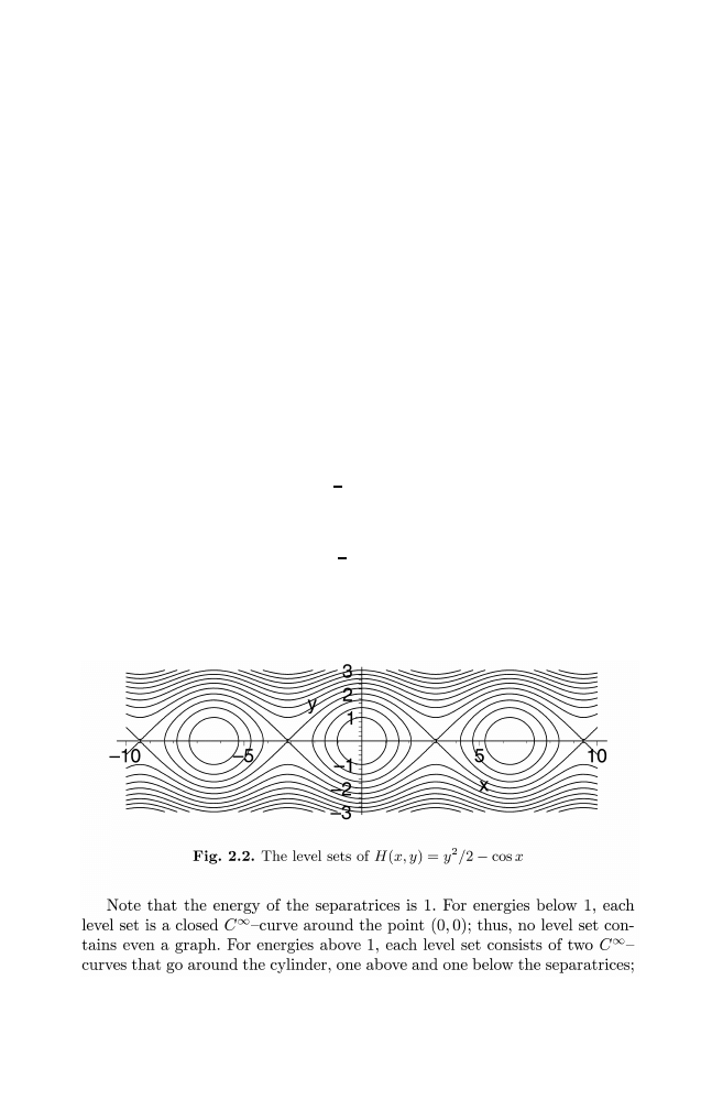
30
2 Mather–Ma˜
n´
e theory
H(x, y) on T
∗
T
n
) is an integral of the corresponding flow. If an invariant
torus is a graph of some closed 1–form ν, then ν must satisfy the equation
H(x, ν
x
) = k = const. Actually, we can restrict ourselves to exact 1–form by
considering L
− ν instead of L; compare Rem. 2.1.3. Finding a smooth exact
invariant torus gr du, where f :
T
n
→ R is some smooth function, is then
equivalent to finding a smooth solution of the (time–independent) Hamilton–
Jacobi equation
H(x, du(x)) = k
(2.10)
Now, smooth solutions of the Hamilton–Jacobi equation will, in general,
not always exist. There is a general theory, developed by Fathi [29], that deals
with Lipschitz continuous solutions of (2.10) and gives another approach to
the critical value. Recall from (2.9) that the critical value is characterized as
the infimum of energy values k such that the sublevel set
{H < k} contains a
smooth solution of (2.10). Moreover, the only energy level that might support
a C
1+Lip
–solution of (2.10) is the level H
−1
(c(L)) where c(L) is the critical
value.
Example 2.2.8. It might be instructive to consider the simplest nontrivial case.
Let L : T
S
1
→ R be the Lagrangian of the mathematical pendulum:
L(x, p) =
1
2
|p|
2
− cos(2πx).
The corresponding Hamiltonian is given by
H(x, y) =
1
2
|y|
2
− cos(2πx)
whose level sets are shown in Fig. 2.2. Since we are in one degree of freedom,
the level sets of H consist of solutions of the Hamiltonian flow, and we end
up with the phase portrait of the pendulum (Fig. 1.3).

2.2 Ma˜
n´
e’s critical value
31
but none of these curves is exact, i.e., the graph of an exact 1–form. The
energy level H
−1
(1), however, is the union of two graphs of differentials of
C
1+Lip
–functions u
±
on
S
1
, namely the upper and lower separatrix.
Therefore, the critical value is 1. In fact, c(L) = max V for any Lagrangian
L(x, p) = 1/2
|p|
2
x
− V (x) on T T
n
.
Given a continuous function u :
T
n
→ R, we write
u
≺ L + c
whenever u(x)
− u(y) ≤ Φ
c
(y, x) for all x, y
∈ T
n
. Here, Φ
c
is the action
potential for the critical value
c := c(L).
Remark 2.2.9. Fathi showed that a function u satisfies u
≺ L + c if, and only
if, it is Lipschitz continuous and fulfills the inequality
H(x, du(x))
≤ c
for almost every x
∈ T
n
; see [29]. In other words, for Lipschitz continuous
functions u, the condition u
≺ L + c is equivalent to u being a subsolution of
the Hamilton–Jacobi equation (2.10).
Note that, by Rademacher’s theorem, Lipschitz functions are differentiable
almost everywhere.
Definition 2.2.10. We say that a continuous function u
+
:
T
n
→ R is a
positive weak KAM solution if u
+
satisfies the following two conditions:
1. u
+
≺ L + c
2. for all x
∈ T
n
there exists an absolutely continuous curve γ
x
+
: [0,
∞) → T
n
such that γ
x
+
(0) = x and
u
+
(γ
x
+
(t))
− u
+
(x) =
t
0
(L + c)(γ
x
+
(s), ˙γ
x
+
(s)) ds
for all t
≥ 0.
Similarly, we say that a continuous function u
−
:
T
n
→ R is a negative
weak KAM solution if u
−
satisfies the following two conditions:
1. u
−
≺ L + c
2. for all x
∈ T
n
, there exists an absolutely continuous curve γ
x
−
: (
−∞, 0] →
T
n
such that γ
x
−
(0) = x and
u
−
(x)
− u
−
(γ
x
−
(
−t)) =
0
−t
(L + c)(γ
x
−
(s), ˙γ
x
−
(s)) ds
for all t
≥ 0.

32
2 Mather–Ma˜
n´
e theory
We denote by
S
±
the set of all positive (respectively, negative) weak KAM
solutions. A pair of functions (u
−
, u
+
) is said to be conjugate if u
±
∈ S
±
and
u
−
= u
+
on the projected Mather set
M.
Fathi’s Weak KAM–Theorem asserts that positive and negative weak
KAM solutions always exist [29]. Moreover, at any point x
0
of differentia-
bility of a weak KAM solution u, Conditions 1 and 2 of the above definition
imply that u satisfies
H(x
0
, du(x
0
)) = c.
In fact, the points x
0
of differentiablity of u
+
(respectively, u
−
) are precisely
those for which the curve γ
x
0
+
(resp. γ
x
0
−
) is unique. The following result [29,
Thm. 5.1.2] states that any function u with u
≺ L+c can be squeezed between
a (unique) pair of conjugate functions.
Theorem 2.2.11. If u :
T
n
→ R is a function such that u ≺ L+c, then there
exists a unique pair of conjugate functions (u
−
, u
+
) such that
u
+
≤ u ≤ u
−
.
Finally, we will need the notion of Peierls barrier which goes back to
Mather [71].
Definition 2.2.12. The Peierls barrier h :
T
n
× T
n
→ R is defined by
h(x, y) := lim inf
T
→∞
Φ
c
(x, y; T ).
The function h is Lipschitz continuous and, by definition, satisfies
h(x, y)
≥ Φ
c
(x, y).
Moreover, the Peierls barrier can be written as
h(x, y) = max
(u
−
,u
+
)
(u
−
(y)
− u
+
(x))
(2.11)
where the maximum is taken over all pairs (u
−
, u
+
) of conjugate functions;
see [29].
2.2.3 The Aubry set
By definition, two conjugate functions u
±
coincide on the projected Mather
set
M. In general, however, there is a bigger set with this property. To define
this set we set
I
(u
−
,u
+
)
:=
{x ∈ T
n
| u
−
(x) = u
+
(x)
}.

2.2 Ma˜
n´
e’s critical value
33
Definition 2.2.13. The projected Aubry set
A is the set of points in T
n
at
which all pairs of conjugate functions coincide:
A :=
(u
−
,u
+
)
I
(u
−
,u
+
)
where the intersection is taken over all pairs of conjugate functions.
It follows from the definition of conjugacy that
M ⊂ A.
In order to define the Aubry set in T
∗
T
n
, we note that the functions u
−
and u
+
are differentiable at every point x
∈ I
(u
−
,u
+
)
with the same derivative.
Moreover, the map
I
(u
−
,u
+
)
x → du
−
(x) = du
+
(x)
∈ T
∗
T
n
is Lipschitz continuous [29, Thm. 5.2.2]. That map defines a set
˜
I
(u
−
,u
+
)
⊂ T
∗
T
n
that projects injectively onto
I
(u
−
,u
+
)
and contains the Mather set. The Aubry
set in T
∗
T
n
is defined as
˜
A
∗
:=
(u
−
,u
+
)
˜
I
(u
−
,u
+
)
where, again, the intersection is taken over all pairs (u
−
, u
+
) of conjugate
functions. As the notation suggests, one can prove that
A = θ( ˜
A
∗
)
where θ : T
∗
T
n
→ T
n
is the canonical projection. As usual, we denote the
preimage of ˜
A
∗
under the Legendre transform by ˜
A and call it the Aubry set
in T
T
n
.
The sets ˜
M and ˜
A are compact and invariant under the Euler–Lagrange
flow φ
t
. It turns out that the Aubry set consists of a distinguished kind of
orbits. To make this precise, we give the following definition due to Ma˜
n´
e.
Recall that c = c(L) denotes the critical value of the Lagrangian L.
Definition 2.2.14. We say that an absolutely continuous curve γ : [a, b]
→
T
n
is semistatic if
A
L+c
(γ) = Φ
c
(γ(a), γ(b)).
An absolutely continuous curve on an infinite interval is called semistatic if
it is semistatic on every finite interval.
Semistatic curves are solutions of the Euler–Lagrange equation because
of their minimizing properties. It is not hard to check that semistatic curves
have energy precisely c.

34
2 Mather–Ma˜
n´
e theory
Definition 2.2.15. An absolutely continuous curve γ : [a, b]
→ T
n
is called
static if it is semistatic and satisfies
Φ
c
(γ(a), γ(b)) + Φ
c
(γ(b), γ(a)) = 0.
An absolutely continuous curve on an infinite interval is called static if it is
static on every finite interval.
In fact, one does not even need to require that a static curve be semistatic.
If one defines static curves by the condition that A
L+c
(γ) =
−Φ
c
(γ(b), γ(a))
then it follows that a static curve is semistatic [21].
The following proposition gives a useful characterization of the Aubry set.
Its proof is well known to experts; nevertheless, we include it for the sake of
completeness.
Proposition 2.2.16. The Aubry set ˜
A consists precisely of those orbits whose
projections to
T
n
are static curves.
Proof. Take (x, v)
∈ ˜
A. We want to show that the curve
γ(t) := τ (φ
t
(x, v))
is a static curve. By the definition of ˜
A and [29, Thm. 5.2.2] we have for any
pair (u
−
, u
+
) of conjugate functions that
u
+
(γ(t))
− u
−
(γ(s)) = u
+
(γ(t))
− u
+
(γ(s)) = A
L+c
(γ
|
[s,t]
)
for all s
≤ t. Using (2.11) we can choose a pair (u
−
, u
+
) of conjugate functions
for which the Peierls barrier h satisfies
h(γ(t), γ(s)) = u
−
(γ(s))
− u
+
(γ(t)).
Therefore, we can estimate
A
L+c
(γ
|
[s,t]
)+Φ
c
(γ(t), γ(s))
≤ u
+
(γ(t))
−u
−
(γ(s))+h(γ(t), γ(s)) = 0. (2.12)
It is easy to show that Φ
c
satisfies the triangle inequality
Φ
c
(x, y)
≤ Φ
c
(x, z) + Φ
c
(z, y)
as well as Φ
c
(x, x) = 0 for all x
∈ T
n
. Hence we have
0 = Φ
c
(γ(s), γ(s))
≤ Φ
c
(γ(s), γ(t)) + Φ
c
(γ(t), γ(s))
≤ A
L+c
(γ
|
[s,t]
) + Φ
c
(γ(t), γ(s))
≤ 0
in view of (2.12). This implies that γ is a static curve.

2.2 Ma˜
n´
e’s critical value
35
Suppose now that γ :
R → T
n
is a static curve. Then γ is a semistatic curve
with energy c, and given s < t and > 0, there exists a curve ¯
γ connecting
γ(t) to γ(s) such that
A
L+c
γ
|
[s,t]
+ A
L+c
(¯
γ)
≤ .
Looking at the loop formed by γ
|
[s,t]
and ¯
γ, we conclude that h(γ(t), γ(t))
≤ 0.
But h(x, x)
≥ Φ
c
(x, x) = 0 for all x
∈ T
n
, and hence h(γ(t), γ(t)) = 0. It
follows from (2.11) that γ(t)
∈ A, and thus (γ(t), ˙γ(t)) ∈ ˜
A, as we wanted to
prove.
We refer the interested reader to [21, 29] for more details on Mather–Ma˜
n´
e
theory.

3
The minimal action and convex billiards
In the classical spectral problem one would like to calculate or estimate the
spectrum of a given Riemannian manifold. The inverse spectral problem asks
the opposite question: how much information about the underlying manifold
is encoded in its spectrum? In other words, to what extent is the geometry
determined by the spectrum? Or, formulated by Kac [49] in his famous title:
can one hear the shape of a drum?
The term “spectrum” can have different meanings here. Either it stands for
the eigenvalue spectrum of the Laplacian, or it means the length spectrum of
the geodesic flow. These two interpretations are not completely independent,
and there are subtle relations via the Poisson relation; see, for instance, [18,
38]. It is known by now that the answer to Kac’ question is negative. There
are whole families of isospectral, non–isometric manifolds; see, e.g., the survey
in [35]. An in–depth survey on positive results concerning the inverse spectral
problem has recently been given by Zelditch in [105].
In the following, we want to consider the inverse spectral problem for
strictly convex domains Ω in
R
2
. The Laplace spectrum with Dirichlet bound-
ary conditions describes the sound you hear when you beat the “drum” Ω. The
notion of length spectrum needs some explanation because Ω has a bound-
ary. By definition, geodesics in a bounded domain Ω are geodesics (in our
case, straight lines) that get reflected at the boundary according to the law
“angle of reflection = angle of incidence”. Such geodesics are often called bro-
ken geodesics. Then the length spectrum consists of the lengths of all closed
(broken) geodesics, together with their multiples.
One way to think of broken geodesics is to image a room Ω lined with
mirrors on its side ∂Ω; broken geodesics are light rays in this mirrored cham-
ber. Another way of looking at broken geodesics is to think of sound travelling
inside the room Ω. Finally, and this is the point of view that we will adopt,
broken geodesics are the trajectories of a billiard “ball” (which is just a point
rather) being played inside the billiard table Ω and going around without
friction.
K.F. Siburg: LNM 1844, pp. 37–57, 2004.
c
Springer-Verlag Berlin Heidelberg 2004

38
3 The minimal action and convex billiards
The main question is whether we can recognize the domain Ω, respectively
its boundary curve, from the knowledge of its length spectrum. One way to
attack this problem is to construct length spectrum invariants (LS–invariants,
for short) and to relate them to geometry. Difficulties may arise in a twofold
way – to prove that a certain geometric quantity is an LS–invariant, or to give
a geometric meaning to some known LS–invariant.
The crucial observation is that, for planar convex domains, one can find
coordinates such that the billiard ball map is a monotone twist map. Moreover,
the length of a closed geodesic is, up to sign, the action of the corresponding
orbit; hence length maximizing geodesics correspond to minimal orbits. This
observation allows us to apply techniques from Aubry–Mather theory. We
will see that the minimal action is invariant under continuous deformations of
the domain that preserve the length spectrum. In addition, many geometric
quantities—such as the lengths and Lazutkin parameters of convex caustics—
can be read off from the minimal action. Note that, once we know that the
minimal action is an LS–invariant, the proof that some geometric quantity
obtained from it is also an invariant becomes trivial. Finally, we show that
the asymptotics of the minimal action is determined by the Dirichlet spectrum
of Ω.
3.1 Convex billiards
Let Ω be a strictly convex domain in
R
2
with C
3
–boundary ∂Ω. As for the
regularity of ∂Ω, we just point out the surprising observation by Halpern [40]
that a C
2
–curve ∂Ω may produce a geodesic flow which is not defined for
all times. Our C
3
–condition guarantees the completeness of the flow. In this
chapter, we will always assume that the length l(∂Ω) of the boundary curve
is normalized to 1.
A broken geodesic in Ω is completely determined by its reflection points,
together with the angles of reflection. The map
φ :
S
1
× (0, π) → S
1
× (0, π)
(s
0
, ψ
0
)
→ (s
1
, ψ
1
)
that associates to a pair (s, ψ)=(arclength on ∂Ω, angle with the positive
tangent) the corresponding data at the next reflection, is called the billiard
map associated to Ω. Let us denote by
h(s, s
) =
−|P (s) − P (s
)
|
the negative Euclidean distance between two points on ∂Ω. Elementary ge-
ometry (see Fig. 3.1) shows that
∂h
∂s
(s
0
, s
1
) = cos ψ
0
∂h
∂s
(s
0
, s
1
) =
− cos ψ
1
(3.1)
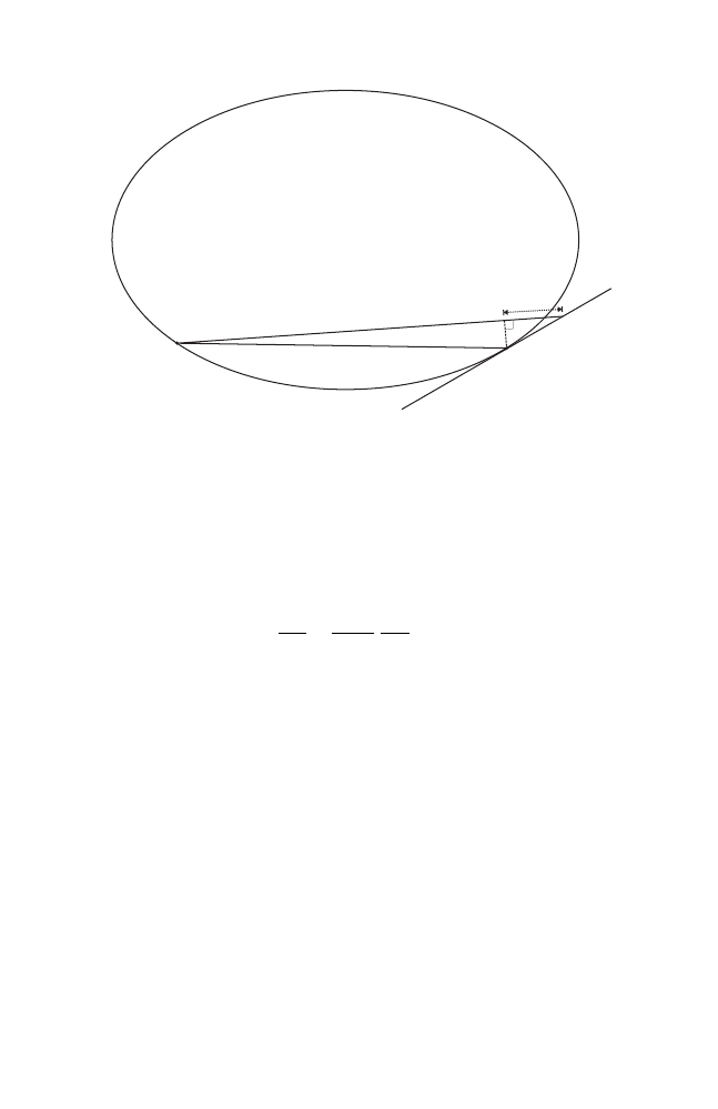
3.1 Convex billiards
39
P(s )
P(s )
0
1
Fig. 3.1. Proof of (3.1)
as well as ∂s
1
/∂ψ
0
> 0.
Thus, if we lift everything to the universal cover and introduce new coor-
dinates (x, y) = (s,
− cos ψ) ∈ R × (−1, 1), we have
y
1
dx
1
− y
0
dx
0
= dh(x
0
, x
1
)
as well as
∂x
1
∂y
0
=
1
sin ψ
0
∂s
1
∂ψ
0
> 0.
This proves the following proposition.
Proposition 3.1.1. In the coordinates (x, y), the billiard map
φ :
R × (−1, 1) → R × (−1, 1)
is a twist map, with the negative Euclidean distance being a generating func-
tion.
Moreover, we may extend the billiard map to the closed strip
S
1
× [−1, 1]
by fixing the boundaries pointwise.
A periodic orbit of the billiard map φ corresponds to a closed (broken)
geodesic inside the domain Ω. In order to distinguish topologically different
closed geodesics, we associate to each periodic orbit its rotation number as
defined in Def. 1.2.2. Let us give a more geometric definition here.
Definition 3.1.2. The rotation number of a periodic billiard trajectory (re-
spectively, a closed broken geodesic) is the rational number
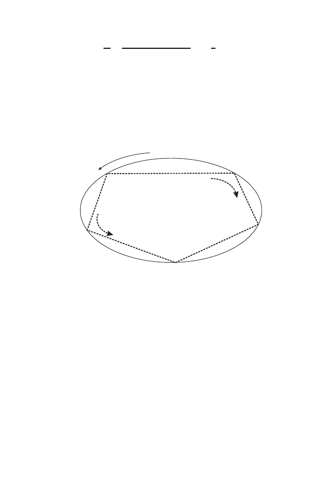
40
3 The minimal action and convex billiards
m
n
=
winding number
number of reflections
∈
0,
1
2
,
where the winding number m
≥ 1 is defined as follows. Fix the positive orien-
tation of ∂Ω and pick any reflection point of the closed geodesic on ∂Ω; then
follow the trajectory and measure how many times it goes around ∂Ω in the
positive direction until it comes back to the starting point.
Note that we restrict ourselves to rotation numbers less than or equal to
1/2, since a closed geodesic with rotation number ω can be seen as one with
rotation number 1
− ω, traversed in the backward direction; see Fig. 3.2.
(fixed) orientation
of the boundary
rotation number 1/5
in this direction
rotation number 4/5
in this direction
Fig. 3.2. Closed geodesics of rotation number 1/5 and 4/5
It was G.D. Birkhoff who introduced convex billiards as a conceptually
simple, yet mathematically complicated, dynamical system. Applied to convex
billiards, Birkhoff’s theorem (Thm. 1.2.4) shows that for every m/n
∈ (0, 1/2]
in lowest terms, there are at least two closed geodesics of rotation number
m/n. In fact, one of them is an inscribed n–gon with winding number m, that
maximizes the perimeter amongst all such n–gons; the other one corresponds
to a saddle point of the length functional.
Example 3.1.3. Consider 2–periodic billiard trajectories in a strictly convex
domain Ω. Geometrically, they correspond exactly to diameters of Ω, i.e.,
segments that meet the boundary at a right angle at both ends. Therefore,
we have n = 2 and m = 1. Already the ellipse is an example with precisely
two 2–periodic billard trajectories, showing that the lower bound in Birkhoff’s
theorem is sharp.
Definition 3.1.4. The marked length spectrum of a strictly convex domain
Ω is the map
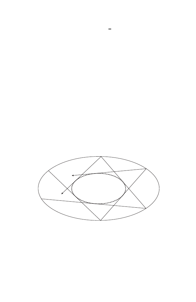
3.1 Convex billiards
41
ML(Ω) : Q ∩
0,
1
2
→ R
that associates to any m/n in lowest terms the maximal length of closed
geodesics having rotation number m/n.
The length spectrum of Ω is defined as the set
L(Ω) := N {lengths of closed geodesics in Ω} ∪ N l(∂Ω).
Note that, due to Birkhoff’s theorem, the marked length spectrum is a
well defined map. Moreover, l(∂Ω) = 1 by our standing assumption that the
boundary length is normalized to 1.
The length spectrum contains information about all closed geodesics, al-
beit in an “unformatted” form. In contrast, the marked length spectrum does
give the labelling by the rotation number but only for the closed geodesics of
maximal length.
Have you ever visited the great basilica in Rome and stood in its huge dome
(42m in diameter)? If you are inside the domed roof and try to communicate
with a friend on the other side of the dome. Rather than shouting into the air,
get close to the circular wall and whisper along the wall – you will be heard
clearly on the other side.
This is the effect of what is usually called a “whispering gallery”. The
sound waves get reflected and travel along the wall, always staying close to it.
In the context of billiards, such a whispering gallery is called a caustic.
Fig. 3.3. A convex caustic
Definition 3.1.5. Let Ω be a strictly convex bounded domain in
R
2
. A convex
caustic is a closed C
1
–curve in the interior of Ω, bounding itself a strictly
convex domain, with the property that each trajectory that is tangent to it
stays tangent after each reflection; see Fig. 3.3.
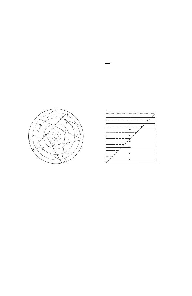
42
3 The minimal action and convex billiards
More generally, a caustic is defined a a continuous curve inside Ω with the
above property; it need not be differentiable, nor bound a convex domain. For
our purposes, however, it is sufficient to restrict ourselves to convex caustics.
Example 3.1.6. The simplest example is given by the disk Ω of perimeter 1.
In the original coordinates (s, ψ), the billiard map is given by
(s
1
, ψ
1
) = (s
0
+
ψ
0
π
, ψ
0
).
Since it preserves the angle, it is an integrable twist map in the coordinates
(x, y) = (s,
− cos ψ). Its phase space is foliated by invariant circles; the phase
portrait is shown in Fig. 3.4. Moreover, the disk Ω is foliated by concentric
circles, each of which is a convex caustic for the circular billiard; see also
Fig. 3.4.
(a) Caustics are concentric cir-
cles
x
y
(b) Phase portrait
Fig. 3.4. The billiard inside a disk
Example 3.1.7. The next simple example is the billiard inside an ellipse. It is
known that this system possesses an integral, i.e., there is a (non–constant)
quantity which is preserved along a trajectory [24]. This integral has the fol-
lowing geometric interpretation.
Consider the billiard inside an ellipse with foci F
1
, F
2
. Then each trajectory
either
1. always intersects the open segment between the two foci, or
2. always passes through the two foci alternately, or
3. never intersects the closed segment between the foci.
In fact, each trajectory, which does not pass through a focal point, is always
tangent to precisely one confocal conic section, either a confocal ellipse (in
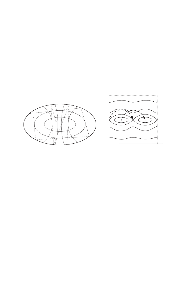
3.1 Convex billiards
43
which case the trajectory never intersects the segment between the foci) or
the two branches of a confocal hyperbola (where the trajectory always in-
tersects the segment between the foci); see Fig. 3.5. The eccentricity of the
corresponding conic section, for example, can be taken as an integral for the
elliptical billiard. For proofs and further remarks, the reader may consult
[24, 101].
Thus, the confocal ellipses inside an elliptical billiard are convex caustics
in accordance with Def. 3.1.5, so the elliptical billiard is foliated by convex
caustics (up to the segment between the foci). The branches of the confocal
hyperbolae can then be seen as caustics in the more general sense mentioned
above.
(a) Caustics are confocal ellipses and hy-
perbolae
x
y
(b) Phase portrait
Fig. 3.5. The billiard inside an ellipse
The phase portrait of an elliptical billiard is also shown in Fig. 3.5. Al-
though it looks like the phase portrait of the pendulum (Fig. 1.3), the dynam-
ics are quite different. The points (0, 0) and (1/2, 0) and its translates do not
represent equilibrium points anymore, but belong to the two–periodic orbits
corresponding one of the half–axes of the ellipse, and similarly for the other
half–axis. Their rotation number is 1/2, which implies that the islands are not
fixed, but “wander”: they are mapped onto each other.
Bounding the islands we see separatrices, corresponding to the orbits
through the foci. The invariant curves above and below the seperatrices rep-
resent the orbits not intersecting the segment between the foci (i.e., being
tangent to confocal hyperbola).
As an aside, we mention here that a famous conjecture, usually attributed
to Birkhoff, states that the elliptical is, in fact, the only convex billiard with
an integral.
44
3 The minimal action and convex billiards
Let us return to the general case of a convex billiard Ω. Suppose for a
moment that the billiard possesses a convex caustic
c. Then one can associate
the following two parameters to
c :
1. its rotation number ω
∈ (0, 1/2), defined as the rotation number of the
circle homeomorphism on
c induced by the geodesic flow via the points of
tangency;
2. its length l(
c).
It turns out that there is a third parameter associated to a convex caustic,
the so–called Lazutkin parameter.
Definition 3.1.8. Let Ω be a convex billiard with a convex caustic
c. Then
the Lazutkin parameter of
c is defined as
Q(
c) = |A − P | + |P − B| − |
AB
|,
where P is any point on ∂Ω and A, B
∈ c are the points of tangency of c seen
from P ; see Fig. 3.6. Moreover,
|
AB
| denotes the length of the caustic’s part
from A to B, where we have oriented the caustic according to the geodesics
touching it.
P
A
B
Fig. 3.6. The Lazutkin parameter of a convex caustic
In fact, if
c is not a caustic but just any closed convex curve inside Ω, the
Lazutkin parameter can be defined in the same manner but may depend on
the point P
∈ ∂Ω. It is independent of P if, and only if, c is a caustic [55, 1].
Therefore, the Lazutkin parameter of a caustic is well defined.
What is the relation between (convex) caustics of a convex billiard Ω and
invariant circles for the corresponding billiard map φ? Certainly, to a convex
caustic in Ω corresponds an invariant circle for the billiard map, i.e. a simply
closed, homotopically nontrivial curve Γ in
S
1
× (−1, 1) with φ(Γ ) = Γ . The
converse, however, is not entirely true. By a theorem of Birkhoff (see [94]

3.2 Length spectrum invariants
45
and the references therein), invariant circles of twist maps are graphs and
therefore do give rise to caustics; but these caustics need neither be convex
nor differentiable.
Finally, one may ask whether convex caustics exist for some arbitrarily
given convex billiard. Lazutkin proved [55] that the billiard map of a convex
billiard with sufficiently smooth boundary possesses a Cantor set of invariant
circles near the boundary, a result which is based on Moser’s twist theorem
on invariant curves [75] (hence the condition on being sufficiently smooth).
Fortunately, invariant circles near the boundary always correspond to caus-
tics which are convex C
1
–curves, so every convex billiard with C
∞
–boundary
possesses (uncountably many) convex caustics according to Def.3.1.5.
3.2 Length spectrum invariants
In this section, we start to investigate which geometric data of a strictly
convex domain Ω
⊂ R
2
are determined by its length spectrum. Recall from
Def. 3.1.4 that the length spectrum is the set
L(Ω) consisting of all multiples
of lengths of closed (broken) geodesics in Ω. The marked length, on the other
hand, is the map associating to every rational m/n the maximal length of a
closed geodesic of rotation number m/n. In order to study the length spectrum
one looks for length spectrum invariants, i.e., quantities that depend only on
the length spectrum; see Def. 3.2.1 below. In particular, we are interested in
invariants that carry some geometric information about the domain Ω.
In general, it is not clear to what extent the marked length spectrum is
determined by the length spectrum, or vice versa. For this reason, we make
the following definition.
Definition 3.2.1. A quantity (number, function, etc.) is called a (marked)
length spectrum invariant if for any two strictly convex domains Ω
0
, Ω
1
⊂ R
2
with the same (marked) length spectrum this quantity is the same.
We will write LS–invariant for length spectrum invariant, and MLS–
invariant for marked length spectrum invariant.
As mentioned before, the notions of LS–invariant and MLS–invariant may
differ. For continuous deformations of smooth (C
∞
) domains, however, one
has the following result.
Proposition 3.2.2. Suppose Ω
s
, s
∈ [0, 1], is a continuous family of strictly
convex domains with C
∞
–boundaries such that
L(Ω
s
) =
L(Ω
0
) for all s. Then
ML(Ω
s
) =
ML(Ω
0
)
for all s.

46
3 The minimal action and convex billiards
Proof. Pick a rational rotation number m/n and a closed geodesic in Ω
s
of ro-
tation number m/n having maximal length. We claim that the corresponding
value
ML(Ω
s
)(m/n) is independent of s.
The chosen geodesic corresponds to a periodic orbit of the corresponding
twist map, respectively, to an (n + 1)–tuple with ξ
0
< ξ
1
< . . . < ξ
n
= ξ
0
+ m
which is a minimum of the finite action functional
H
s
(ξ
0
, . . . , ξ
n+1
) =
n
i=0
h
s
(ξ
i
, ξ
i+1
),
where the generating function h
s
is nothing but the negative length function
in Ω
s
. By Sard’s Theorem, the critical values of H
s
, i.e., the values of
L(Ω
s
),
form a set of Lebesgue measure zero. In general, the maxima of a family of
smooth functions depend continuously on the parameter. In our case, they lie
in a set of Lebesgue measure zero, so they must stay constant.
This means that the maximal length of closed geodesics having a fixed
rotation number m/n does not depend on s. Hence the functions
ML(Ω
s
), s
∈
[0, 1], are all the same.
Corollary 3.2.3. For continuous deformations of smooth strictly convex do-
mains Ω
s
, MLS–invariants are also LS–invariants. In other words, if a certain
quantity stays invariant under deformations with
ML(Ω
s
) =
ML(Ω
0
), it is
also invariant under deformations with
L(Ω
s
) =
L(Ω
0
).
We have seen in the previous section that the billiard map associated to a
convex domain Ω is a monotone twist map on
S
1
×(−1, 1) generated by h, the
negative distance between points on ∂Ω. Therefore, closed geodesics of maxi-
mal length correspond to minimal orbits, and the marked length spectrum is
essentially nothing but the minimal action; more precisely,
α
m
n
=
−
1
n
ML(Ω)
m
n
(3.2)
for every m/n
∈ (0, 1/2] in lowest terms.
This simple observation turns out quite fruitful because it implies the
following principle.
Main Principle. Every quantity that can be calculated from the minimal
action is, by tautology, a marked length spectrum invariant.
Remark 3.2.4. One of the main advantages of this principle is that the actual
proof that a certain quantity is a MLS–invariant becomes trivial, once it is
clear how the quantity can e calculated from the minimal action; we will see
applications of this remark in the following sections.
Vice versa, we see from the identity (3.2) that every MLS–invariant must
be hidden in the minimal action—the only question is how. Let us formulate
the above principle as a theorem.
3.2 Length spectrum invariants
47
Theorem 3.2.5. The minimal action α : [0, 1]
→ R for the billiard map
of a strictly convex C
3
–domain Ω
⊂ R
2
is a complete MLS–invariant, i.e.,
ML(Ω
0
) =
ML(Ω
1
) if and only if α
0
= α
1
.
Moreover, α is a strictly convex function on [0, 1], symmetric with respect
to the point 1/2, and three times differentiable at the boundary points with
α
(0) =
−l(∂Ω) = −1.
Proof. The first assertion follows from (3.2) and the continuity of α. The strict
convexity is contained in Proposition 1.3.7; the symmetry property is obvious.
For the last part, we make use of a special choice of coordinates near the
boundary
{ψ = 0} which is due to Lazutkin [55, 56]. Namely, let us introduce
ξ = C
s
0
ρ
−2/3
(τ ) dτ
,
η = 4Cρ
1/3
(s) sin
ψ
2
where ρ
∈ C
1
(
S
1
,
R) is the radius of curvature and C = (
1
0
ρ
−2/3
)
−1
. Then
{ψ = 0} corresponds to {η = 0}, and the invariant symplectic form sin ψ dψ ∧
ds takes the form
1
4C
3
η dη
∧ dξ = d
1
8C
3
η
2
dξ
.
Moreover, one calculates that
φ(ξ, η) = (ξ + η, η) +
O(η
2
)
as η
→ 0. Hence φ is a perturbation of the integrable twist map (ξ, η) →
(ξ + η, η), and we obtain for the generating function
1
h(ξ
0
, ξ
1
) =
1
24C
3
(ξ
1
− ξ
0
)
3
+
O((ξ
1
− ξ
0
)
4
)
as ξ
1
−ξ
0
→ 0. Prop. 1.3.8 implies that the minimal action—in the coordinates
ξ, η—can be written as
α
ξ,η
(ω) =
1
24C
3
ω
3
+
O(ω
4
)
as ω
→ 0.
Transforming back to the coordinates x, y means adding the linear term
−ω to the action [67] because the cohomology class [y dx − (8C
3
)
−1
η
2
dξ] is
−1; the latter is due to the fact that the boundary {ψ = 0} corresponds to
{y = −1} respectively {η = 0}. Summarizing, we have for the minimal action
α(ω) =
−ω +
1
24C
3
ω
3
+
O(ω
4
)
(3.3)
as ω
→ 0. By symmetry, an analogous formula holds near ω = 1.
1
Note that the exponent in the first term is 3, due to the nonstandard form of the
symplectic form.
48
3 The minimal action and convex billiards
Recall from (1.7) that the convex conjugate of α is defined as α
∗
(I) =
max
ω
[ωI
− α(ω)] with (α
∗
)
(α
(ω)) = ω. Hence, in view of Theorem 3.2.5,
the domain of definition of α
∗
is the interval [
−1, 1]. By way of illustration,
let us calculate the minimal action and its convex conjugate in the simplest
example.
Example 3.2.6. Take Ω to be the disk of perimeter 1 in
R
2
. The billiard map
is integrable and given by (s
1
, ψ
1
) = (s
0
+ ψ
0
/π, ψ
0
) with generating function
h(s, s
) =
−
1
π
sin π(s
− s
).
The whole phase space is foliated by invariant circles
{y = const.}, and
the minimal action is just
α(ω) =
−
1
π
sin πω.
In view of the identity sin arccos(
−x) =
√
1
− x
2
, its convex conjugate is
α
∗
(I) =
1
π
arccos(
−I) · I +
1
− I
2
∈ [0, 1]
for I
∈ [−1, 1]. The graphs of α and its convex conjugate α
∗
are depicted in
Fig. 3.7.
–0.4
–0.3
–0.2
–0.1
0
0.1
y
0.2
0.4
0.6
0.8
1
x
(a) The minimal action
α
0
0.2
0.4
0.6
0.8
1
y
–1
–0.8 –0.6 –0.4 –0.2
0.2
0.4
0.6
0.8
1
x
(b) The convex conjugate
α
∗
Fig. 3.7. The minimal action for the disk and its convex conjugate
The asymptotics for ω
→ 0 and I → −1, respectively, are as follows:
α(ω) =
−ω +
π
2
6
ω
3
−
π
4
120
ω
5
+
O(ω
7
)
α
∗
(I) =
√
2
π
2
3
(I + 1)
3/2
+
1
30
(I + 1)
5/2
+
3
560
(I + 1)
7/2
+
O((I + 1)
9/2
)
α can be extended to an odd smooth function on
R. α
∗
has a singularity of
order 3/2 at I =
−1; the function (α
∗
)
2/3
is smooth.

3.2 Length spectrum invariants
49
If we ask whether the minimal action can be recovered from the length
spectrum instead of the marked length spectrum, we have the following result
for continuous deformations.
Corollary 3.2.7. For continuous deformations of smooth strictly convex do-
mains, α is an LS–invariant function on [0, 1].
Proof. Immediate from Corollary 3.2.3.
Finally, we point out that the minimal action is actually invariant under
arbitrary symplectic (i.e., area–preserving) coordinate changes in the phase
space. For, by (3.11), the actions of periodic orbits are symplectically invari-
ant, and they determine α.
3.2.1 Classical invariants
What kind of geometric data can be recovered from the (marked) length
spectrum? It is well known, for instance, that the perimeter and the diameter
of the domain Ω are invaraints of the spectrum, a fact which follows readily
from the Main Principle.
Proposition 3.2.8. The boundary length l(∂Ω), the diameter diam Ω, and
the curvature integral
ρ
−2/3
are MLS–invariants.
Proof. This is an immediate consequence of our Main Principle, together with
(3.3),since l(∂Ω) =
−α
(0), diamΩ =
−α(1/2), and (
ρ
−2/3
)
3
= 4α
(0).
Remark 3.2.9. In view of Cor. 3.2.7, the above quantities are LS–invariants
for continuous deformations of smooth strictly convex domains.
Are there other geometric data hidden in the minimal action? The follow-
ing theorem shows that the parameters connected to a convex caustic can be
read off from the minimal action.
Theorem 3.2.10. Let Ω be a strictly convex C
3
–domain in
R
2
, and suppose
that
c
ω
is a convex caustic of rotation number ω. Then the length of
c
ω
and
its Lazutkin parameter are given by
l(
c
ω
) =
−α
(ω)
and
Q(
c
ω
) = α
∗
(α
(ω)).
Proof. Call T (s) and N (s) the unit tangent vector and unit inward normal, re-
spectively, at a point P (s)
∈ ∂Ω, and set U(s) = cos ψ(s)T (s) + sin ψ(s)N(s);
here, ψ(s)
∈ (0, π/2) is the unique angle such that the ray from P (s) having
direction U (s) touches
c
ω
. Then there is a function τ (s) such that

50
3 The minimal action and convex billiards
A(s) = P (s) + τ (s)U (s)
∈ c
ω
and
˙
A(s) = T (s) + ˙τ (s)U (s) + τ (s) ˙
U (s)
U(s).
Since ˙
A(s)
= 0, we can write
| ˙
A(s)
| = ˙
A(s), U (s)
= cos ψ(s) + ˙τ(s)
so that
l(
c
ω
) =
S
1
| ˙
A
| ds =
S
1
cos ψ ds =
−
Γ
ω
y dx =
−α
(ω)
by Proposition 1.3.7.
By definition of the Lazutkin parameter (see Fig. 3.6), we have
(N + 1)Q(
c
ω
) =
|A
1
− P
1
| +
N
i=1
|P
i
− P
i+1
| + |P
N +1
− B
N +1
| −
N +1
i=1
|
A
i
B
i
|
for N
≥ 1. Hence
Q(
c
ω
) = lim
N
→∞
1
N
N
i=1
|P
i
− P
i+1
| − lim
N
→∞
1
N
N
i=1
|
A
i
B
i
|
=
−α(ω) − ωL(c
ω
)
= ωα
(ω)
− α(ω)
= α
∗
(α
(ω))
Corollary 3.2.11. The length and Lazutkin parameter of a convex caustic are
MLS–invariants, respectively, LS–invariants under continuous deformations.
Remark 3.2.12. The result that lengths and Lazutkin parameters of convex
caustics are spectrally determined is due to Amiran [2]. The above proof,
however, is new.
Remark 3.2.13. In view of Theorem 3.2.10, one might call
−α
and α
∗
the
generalized “length” and “Lazutkin parameter”, even if there is no convex
caustic of the corresponding rotation number.
Given a convex caustic
c, one can reconstruct ∂Ω by wrapping a string of
length l(
c) + Q(c) around c, pulling it tight, and going along c. These “string
length parameters” of convex caustics are, of course, also MLS–invariants of
the domain Ω.
The following result shows how analytical properties of α translate into
geometric properties of Ω.

3.2 Length spectrum invariants
51
Proposition 3.2.14. Let Ω
⊂ R
2
be a strictly convex C
3
–domain with as-
sociated minimal action α : [0, 1]
→ R. Then the following statements are
equivalent:
1. α is differentiable at the point 1/2;
2. ∂Ω is a curve of constant width.
Proof. The differentiability of α at 1/2 is, in view of Thm. 1.3.7, equivalent to
the existence of an invariant circle consisting entirely of minimal 2–periodic
orbits, i.e., diameters of the same length.
Another well known fact is the spectral rigidity of the disk, i.e., that the
disk is completely determined by its spectrum. In our context, we have the
following rigidity result.
Theorem 3.2.15. Let Ω
⊂ R
2
be a strictly convex C
3
–domain with associated
minimal action α : [0, 1]
→ R. Then the following statements are equivalent:
1. α is differentiable;
2. α is analytic;
3. Ω is a disk.
Proof. Since 3.
⇒ 2. ⇒ 1. in view of Example 3.2.6, it suffices to show 1. ⇒ 3.
According to Thm. 1.3.7, the differentiability of α at the point 1/2 is
equivalent to the existence of an invariant circle consisting of minimal periodic
orbits. Taking limits of these curves, we obtain invariant circles for all rotation
numbers, consisting entirely of minimal orbits.
We claim that they foliate the phase space. Indeed, if there was a gap, its
boundary curves would necessarily have the same rotation number (otherwise,
there would be rotation numbers without invariant circles). But this is impos-
sible, due to the graph property of the set of minimal orbits in Theorem 1.3.4.
Now the assertion follows from Bialy’s result [9] that the only billiard
whose phase space is foliated by invariant circles is a circular one.
Remark 3.2.16. We conjecture that the statement “α is differentiable near the
point 1/2
⇒ Ω is a disk” is true, which would mean that the differentiability
of a minimal action, stemming from a strictly convex billard, near 1/2 already
implies its global differentiability.
Corollary 3.2.17. Suppose Ω is a strictly convex C
3
–domain with the same
marked length spectrum as the disk of the same perimeter. Then Ω is a disk.
Remark 3.2.18. In view of Corollary 3.2.3, we have the following rigidity result
for deformations: any continuous deformation of the disk (inside the class of
smooth convex domains) that preserves the length spectrum must be trivial.
Remark 3.2.19. Corollary 3.2.17 has an analogue in differential geometry: a
Riemannian 2–torus, having the same marked length spectrum as a flat torus,
is flat [7, Thm. 6.1].

52
3 The minimal action and convex billiards
3.2.2 The Marvizi–Melrose invariants
So far, we have considered the most general case of domains with C
3
–
boundaries where we do not know, for instance, whether there are any con-
vex caustics at all. If we assume smooth enough boundaries, however, then
Moser’s twist theorem [75] can be applied and guarantees the existence of a
Cantor family of convex caustics that accumulate at the boundary ∂Ω; this
was first proven by Lazutkin [55]. From now on, we assume that Ω is smooth
(C
∞
). Then there is the following KAM–theorem by Kovachev and Popov
[52, Thm. 2] which is based on the work of P¨
oschel [89].
Theorem 3.2.20. Let Ω be a smooth strictly convex domain of unit boundary
length. Then there are symplectic coordinates (θ, I) near
{y = −1} ↔ {I =
−1} such that the billiard map φ : (θ
0
, I
0
)
→ (θ
1
, I
1
) is generated by
S(θ
0
, I
1
) = θ
0
I
1
+ K(I
1
)
3/2
+ R(θ
0
, I
1
),
i.e.,
I
0
= ∂
1
S = I
1
+ ∂
1
R
θ
1
= ∂
2
S = θ
0
+
3
2
K(I
1
)
1/2
K
(I
1
) + ∂
2
R
(3.4)
Here, K
∈ C
∞
(
R, R) with K(−1) = 0, K
(
−1) > 0, and R ∈ C
∞
(
R
2
,
R)
is 1–periodic in the first variable. Moreover, there exists a Cantor set
C
∗
⊂
[
−1, −1 +
∗
) with
−1 ∈ C
∗
, where
∗
> 0 is some small number, such that
R
≡ 0 on R × C
∗
.
We see that the perturbation term R vanishes on
R × C
∗
with all its
derivatives. Each curve
R × {I}, I ∈ C
∗
, gives rise to an invariant circle for
the billiard map on which it is conjugated to the rigid rotation
(θ, I)
→ (θ + ω, I)
(3.5)
with ω = 3/2K(I)
1/2
K
(I). Since these invariant circles lie near the boundary,
they correspond to a Cantor set of convex caustics near and accumulating at
∂Ω.
In view of (3.5), θ
0
I
1
+ α
∗
(I
1
) generates φ : (θ
0
, I
0
)
→ (θ
1
, I
1
) on the
Cantor set
R×C
∗
of invariant circles accumulating at
R×{−1}. We also know
from Theorem 3.2.20 that φ is generated by S = θ
0
I
1
+ K(I
1
)
3/2
+ R(θ
0
, I
1
),
where K is smooth and R vanishes with all its derivatives on
R × C
∗
. Since
α
∗
(
−1) = 0 = K(−1), we must have that
α
∗
(I) = K(I)
3/2
(3.6)
for all I
∈ C
∗
. Thus, α
∗
yields a generating function for φ, restricted to a
Cantor set of invariant KAM–circles.
The smooth function K can be written as
K(I) = K
(
−1) · (I + 1) + O((I + 1)
2
)
(3.7)

3.2 Length spectrum invariants
53
with K
(
−1) > 0. Combining (3.6) and (3.7) we obtain that
α(ω) = a
1
ω + a
3
ω
3
+
O(ω
5
)
is smooth on the Cantor set
C =
3
2
K(I)
1/2
K
(I)
| I ∈ C
∗
(3.8)
containing 0.
Let us return to the original question which geometric data can be re-
covered from the (marked) length spectrum. Concerning the lengths and
Lazutkin parameters of convex caustics—whose existence is now guaranteed
by Thm. 3.2.20— Cor. 3.2.11 immediately implies the following assertion.
Theorem 3.2.21. The function ω
→ (l(c
ω
), Q(
c
ω
)), defined on a Cantor set
in [0, 1] containing 0 and 1, is an MLS–invariant, respectively an LS–invariant
under continuous deformations.
Remark 3.2.22. Again, we point out that Thm. 3.2.21 is not new: it is the
main result in [88]. Popov’s proof, however, relies on the existence of invariant
KAM–circles, and a good part of it is hard analysis. Our approach is simpler
and shows that the invariance property of the caustic parameters is definitely
not a phenomenon inside KAM–theory.
In the smooth case, Theorem 3.2.10 also implies a functional dependence
of l(
c) and Q(c).
Theorem 3.2.23. There is a formal power series expansion
l = 1 +
k
≥1
b
k
Q
2k/3
as Q
→ 0, whose coefficients are MLS–invariants, respectively LS–invariants
under continuous deformations.
Proof. l(
c
ω
) =
−α
(ω) and Q(
c
ω
)
2/3
= α
∗
(α
(ω))
2/3
= K(α
(ω)) are smooth
functions on
C with K
(
−1) > 0. The claim follows from the implicit function
theorem.
Remark 3.2.24. Cor. 3.2.23 was first stated explicitly in [2, (3.1)]. It follows,
however, already from formulae obtained by Lazutkin, namely (1.11) and
(1.12) in [55], where he expresses the length and his parameter in terms of the
rotation number.
Let us go on and see if there are other spectral invariants hidden in the
minimal action. In 1982, Marvizi and Melrose [63] defined a sequence of MLS–
invariants by investigating an integrable approximation of the billiard map

54
3 The minimal action and convex billiards
near the boundary. The Marvizi–Melrose invariants are given by the asymp-
totics of a so–called interpolating Hamiltonian. By definition, an interpolating
Hamiltonian is a smooth function ζ on
S
1
× [−1, 1], whose time–ζ
1/2
–map is
the billiard map, up to a diffeomorphism that fixes the boundary to infinite
order. The integral invariants are then defined as the Taylor coefficients of
J (r) :=
1
ζ
(ζ
−1
(r))
(3.9)
at r = 0 for any interpolating Hamiltonian ζ in action–angle–variables.
We claim that, in the context of minimal action, we can find a quite simple
interpolating Hamiltonian. Indeed, from (3.4) and (3.6), we see that
ζ(I) :=
3
2
2/3
K(I) =
3
2
α
∗
(I)
2/3
is an interpolating Hamiltonian, at least on a Cantor set containing the bound-
ary. Since the Taylor coefficients of (3.9) at the boundary point r = 0 only
depend on the behaviour of ζ(I) on any sequence accumulating at 0, they only
depend on the Taylor coefficients of α
∗
at the corresponding boundary point
−1. Summarizing, we obtain the following result.
Theorem 3.2.25. The integral invariants of Marvizi and Melrose are alge-
braically equivalent to the Taylor coefficients of α
∗
at
−1.
Marvizi and Melrose [63] go further and prove an asymptotic formula for
the lengths of closed geodesics which is then shown to be spectrally deter-
mined. In order to integrate this formula into our context, we consider a
closed geodesic g
mn
of rotation number m/n. Its length is given by
l(g
mn
) =
−
g
mn
h.
(3.10)
We want to rewrite this in (θ, I)–coordinates and relate it to the generating
function S(θ
0
, I
1
) from Theorem 3.2.20. We have the following transforma-
tions:
Φ : (θ, I)
→ (x, y) with
Φ
∗
(y dx)
− I dθ = dH
Ψ = Φ
−1
◦ φ ◦ Φ
θ
1
dI
1
+ I
0
dθ
0
= dS
with
S = θ
0
I
1
+ K(I
1
)
3/2
+ R(θ
0
, I
1
)
A straightforward calculation shows that the generating function transforms
according to the formula
Ψ
∗
(I dθ)
− I dθ = d(h ◦ Φ + H − H ◦ Ψ).
(3.11)
On the other hand, we can write the left hand side as

3.2 Length spectrum invariants
55
I
1
dθ
1
− I
0
dθ
0
= (
−θ
1
dI
1
− I
0
dθ
0
) + (θ
1
dI
1
+ I
1
dθ
1
)
=
−dS +
∂S
∂I
1
dI
1
+ I
1
d(
∂S
∂I
1
)
= d
I
1
∂S
∂I
1
− S
= dS
∗
From this we conclude that
−h ◦ Φ = H − H ◦ Ψ − S
∗
+ const.
Summed over a closed orbit, the term H
− H ◦ Ψ adds to zero, so (3.10) yields
1
n
l(g
mn
) =
1
n
g
mn
−S
∗
+
const.
n
.
Since S
∗
= (K(I)
3/2
)
∗
+ I ∂R/∂I
− R has the same Taylor series at the
boundary point as (K(I)
3/2
)
∗
, which coincides on
S
1
× C with (α
∗
)
∗
= α,
we see that l(g
mn
)/n has the same Taylor series for n
→ ∞ as −α. Loosely
speaking, all closed geodesics become minimal as they approach ∂Ω. More
precisely,
l(g
mn
) = m +
k
≥1
c
mk
n
−2k
where
c
mk
=
−
m
2k+1
(2k + 1)!
α
(2k+1)
(0).
(3.12)
This formula implies the following
Theorem 3.2.26. If Ω is smooth, the asymptotics of the length spectrum as
n
→ ∞ are equivalent to that of the minimal action as ω → 0.
3.2.3 The Gutkin–Katok width
Another application of Theorem 3.2.5 concerns regions in Ω which are free of
convex caustics. Gutkin and Katok gave estimates for their area in terms of
the geometry of Ω. In particular, they proved [39, Prop. 1.3] that a convex
caustic
c
ω
with rotation number ω cannot lie too far from the boundary:
max
P
∈c
ω
d(P, ∂Ω) <
diamΩ
· Q(c
ω
).
See Fig. 3.8 for an illustration.
We will see that the Gutkin–Katok width
diamΩ
· Q(c
ω
) has an MLS–
invariant interpretation. Indeed, in view of Prop. 3.2.8 and Theorem 3.2.10,
this number can also be written as
diamΩ
· Q(c
ω
) =
−α(1/2) · α
∗
(α
(ω)).
According to our Main Principle, this proves the following result.

56
3 The minimal action and convex billiards
no caustic of rotation
number
in this region
w
Fig. 3.8. The Gutkin–Katok width
Theorem 3.2.27. Suppose Ω
0
, Ω
1
are two strictly convex C
3
–domains with
the same marked length spectrum. Then, for a fixed rotation number ω, every
convex caustic
c
ω
in Ω
0
, respectively Ω
1
, is contained in a strip around ∂Ω
0
,
respectively ∂Ω
1
, of one and the same width.
3.3 Laplace spectrum invariants
As already mentioned in the introduction, there is a relation between the
length spectrum
L(Ω) of a strictly convex domain and the spectrum of the
Laplacian with Dirichlet boundary conditions:
u = λ
2
u
in Ω
u = 0
on ∂Ω
(3.13)
Indeed, due to a Poisson relation for compact Riemannian manifolds with
geometrically convex boundary [38], the expression
σ(t) =
λ
2
∈spec
cos λt
is well defined as a distribution, which is smooth away from
L(Ω) [3]. More
precisely, if T > 0 is in the singular support of σ then T lies in the length
spectrum of Ω.
Conversely, whether some given T
∈ L(Ω) belongs to the singular support
of σ, depends on possible cancellations of singularities stemming from different
closed geodesics of the same length. It is known [38] that T lies in the singular
support of sigma if there is exactly one closed geodesic of length T , whose
Poincar´
e map does not have an eigenvalue 1. Marvizi and Melrose [63] showed
that a much weaker non–coincidence condition on Ω suffices to conclude that
almost all maximal lengths of geodesics having rotation number 1/n lie in

3.3 Laplace spectrum invariants
57
the singular support of σ. Popov [88] generalized this to geodesics of rotation
number m/n with m > 1, provided (m, n) is “near” the Cantor set described in
(3.8). In particular, that non–coincidence condition is satisfied by all curvature
functions in a C
1
–neighbourhood of the constants.
Thus, the values α(1/n), respectively α(m/n), with sufficiently large n are
spectral invariants of the domain. This is also true for the coefficients c
1k
in
(3.12), and hence for the Taylor coefficients of
−α at 0. Therefore we can state
the following result which is an analogue of [63, Thm. 7.4].
Theorem 3.3.1. Suppose Ω
⊂ R
2
is a smooth strictly convex domain with
unit boundary length, such that 1 is not a limit point of lengths of closed
geodesics having fixed rotation number m/n with m > 1. Then the Taylor
series of the minimal action at 0 is completely determined by the Dirichlet
spectrum (3.13).
Applying Popov’s more general result, one can show that also the values
of α on the Cantor set
C (and hence all the caustic parameters L(c) and Q(c))
are spectral invariants under the non–coincidence condition in [88, (6.1)].
For an exhaustive treatise on the inverse (Laplace) spectral problem prob-
lem we refer to the survey by Zelditch [105].

4
The minimal action near fixed points and
invariant tori
When investigating a dynamical system it is often a first important step to
transform it into a form as simple as possible. If the system belongs to some re-
stricted class these normal forms should be invariant under the corresponding
invariance transformations.
In classical mechanics, the class under consideration consists of Hamilto-
nian systems, respectively symplectic transformations. We consider a symplec-
tic map near a fixed point (in two dimensions), respectively, near an invariant
torus (in arbitrary dimensions). Under certain nondegeneracy conditions on
the linearization of the map , G.D. Birkhoff constructed a normal form that
is invariant under symplectic coordinate changes. This Birkhoff normal form
describes an integrable approximation of the original map. Its asymptotics at
the fixed point define a set of symplectic invariants; for obvious reasons, we
call these Birkhoff invariants asymptotic.
The goal of this chapter is the construction of a new local symplectic invari-
ant that, in particular, includes the asymptotic Birkhoff invariants. To do so,
we will associate to the germ of a symplectic map at a fixed point/invariant
torus the germ of its minimal action. This is symplectically invariant and,
in contrast to the Birkhoff normal form, reflects part of the dynamical be-
haviour in a neighbourhood of the fixed point/invariant torus. We show that
the classical Birkhoff invariants are encoded in the minimal action as the Tay-
lor coefficients of its convex conjugate. Moreover, in the integrable case, the
minimal action determines the map completely, a fact which is also not true
for the Birkhoff normal form (unless the map is analytic).
Symplectic mappings near a fixed point appear as Poincar´
e section maps of
a closed trajectory. We explain this for the geodesic flow on a compact surface.
It turns out that the minimal action depends only on the length spectrum of
the Riemannian manifold. Therefore, the minimal action is a new local length
spectrum invariant for compact two–dimensional manifolds.
In the final section we investigate the role of the minimal action near an
invariant torus of a symplectic map.
K.F. Siburg: LNM 1844, pp. 59–80, 2004.
c
Springer-Verlag Berlin Heidelberg 2004

60
4 The minimal action near fixed points and invariant tori
4.1 The minimal action near plane elliptic fixed points
We consider an area–preserving diffeomorphism φ of the plane in the vicinity
of a fixed point. We can shift the fixed point into the origin, so we assume that
φ(0) = 0. Moreover, we are only interested in the local behaviour of φ near
0. Therefore, we call two diffeomorphisms equivalent if they coincide on some
open neighbourhood of the origin. In other words, we consider the equivalence
class of φ, i.e., we consider the germ of a symplectic diffeomorphism at the
fixed point 0
∈ (R
2
, Ω) where Ω is some area form on
R
2
. In the following,
whenever we pick a representative φ : U
→ R
2
, we assume that U is a simply
connected neighbourhood of 0; this is no loss of generality. Then, by Poincar´
e’s
Lemma, the symplectic form Ω is exact, i.e., there is a 1–form λ with Ω = dλ.
Suppose for a moment that there is a point p
∈ U \ {0} whose iterates
p
i
= φ
i
(p) exist for all i
∈ Z. We want to define the average action and the
rotation number of the orbit (p
i
)
i
∈Z
. Since φ is symplectic, the 1–form φ
∗
λ
−λ
on U is closed, hence exact:
φ
∗
λ
− λ = dS.
Definition 4.1.1. Let φ : U
→ R
2
be a symplectic diffeomorphism, and λ be
a (local) primitive of the area form Ω.
Any function S : U
→ R satisfying φ
∗
λ
− λ = dS is called a generating
function for φ. Any two generating functions differ by some additive constant,
and we normalize S by setting S(0) = 0; this makes the generating function
unique.
If (p
i
)
i
∈Z
is an orbit of φ then the average action of (p
i
) is defined as
A((p
i
)) := lim
N
→∞
1
2N
N
−1
i=−N
S(p
i
)
if this limits exists.
Remark 4.1.2. As an aside, we remark that the normalization of the generating
function is in accordance with setting H(t, 0) = 0 when H is a Hamiltonian
whose flow generates φ and leaves 0 fixed; for, then the generating function
λ
− H dt vanishes at 0.
Lemma 4.1.3. The average action does not depend on the choice of the 1–
form λ. Moreover, it is invariant under local symplectic coordinate changes Φ
fixing the origin.
Proof. We claim that the definition of the average action does not depend on
the choice of the 1–form λ. Indeed, taking another 1–form λ
with dλ
= dλ =
Ω, the closed 1–form λ
− λ is exact: λ
− λ = dF . The new (normalized)
generating function is given by S
= S + φ
∗
F
− F . But the average of φ
∗
F
over an orbit is the same as that of F , so the summation of φ
∗
F
− F over the
orbit vanishes. This proves our first claim.
4.1 The minimal action near plane elliptic fixed points
61
Moreover, we claim that the average action is invariant under local sym-
plectic coordinate changes Φ fixing the origin. Such a transformation Φ is
generated by some function F , due to Poincar´
e’s Lemma. Then a short
calculation shows that the generating function for Φ
◦ φ ◦ Φ
−1
is given by
Φ
∗
S + F
− (Φ ◦ φ ◦ Φ
−1
)
∗
F . Now the claim follows by the same argument as
above.
Next, we want to define the rotation number of an orbit (p
i
)
i
∈Z
in U
\ {0}.
Roughly speaking, this is its average winding number around the origin. More
precisely, we introduce polar coordinates on
R
2
\ {0} = S
1
× (0, ∞), and lift
φ : U
\ {0} → R
2
\ {0} to a map
φ which is then defined on some strip
in the universal cover
R × (0, ∞) of S
1
× (0, ∞). Since φ is an orientation–
preserving diffeomorphism,
φ is a diffeomorphism of degree 1. Given an orbit
(
p
i
) of
φ projecting onto (p
i
) and a natural number N , we choose a curve
Γ : [
−N, N] → R × (0, ∞) with
Γ (i) =
p
i
. Call Γ : [
−N, N] → R
2
\ {0} the
projection of
Γ , and close it up to a closed curve Γ
N
by adding a “short”
piece (whose lift upstairs lies inside one fundamental domain); see Fig. 4.1.
0
p
p
p
-N
0
N
G
N
p
p
-1
1
Fig. 4.1. The rotation number of an orbit (p
i
)
i∈Z
Then we define the rotation number of (
p
i
) to be
ρ((
p
i
),
φ) := lim
N
→∞
1
2N
[Γ
N
]
∈ H
1
(
R
2
\ {0}, R)
if this limit exists. Clearly, if we fix the lift
φ, the class ρ does not depend
on the particular choice of (
p
i
) and Γ
N
. Moreover, choosing a different lift φ
means adding the class [φ
−
φ] of the deck transformation φ
−
φ. Finally, we
have a canonical identification H
1
(
R
2
\ {0}, R) = R if we take as generator of
H
1
(
R
2
\ {0}, R) the class represented by the positively oriented unit circle.

62
4 The minimal action near fixed points and invariant tori
Definition 4.1.4. The rotation number of an orbit (p
i
)
i
∈Z
contained in U
\
{0} is defined as the real number
ρ((p
i
)) := ρ((
p
i
),
φ),
where
p
i
and
φ are defined as above. It is well defined up to integer shifts, and
invariant under conjugation by homeomorphisms.
Analogous to Aubry–Mather theory, we introduce the following variational
principle for the symplectic map φ : U
\{0} → R
2
\{0}. Having fixed some lift
φ of φ, we denote by α(ω) the infimum of average actions of orbits in U
\ {0}
with rotation number ω where, as usual, the infimum over the empty set is
∞.
Definition 4.1.5. Consider the germ of a symplectic diffeomorphism at the
fixed point 0. Then the minimal action is defined as the function
α :
R → (−∞, ∞]
ω
→ inf{A((p
i
))
| ρ((p
i
)) = ω
}
(4.1)
taking the infimum of average actions over all orbits of a given rotation num-
ber.
The minimal action is well defined up to additive integers in the rotation
number ω. What are the invariance properties of the minimal action?
Proposition 4.1.6. The minimal action is invariant under (local) symplectic
diffeomrophisms.
Proof. In view of Lemma 4.1.3, the average action is invariant under symplec-
tic coordinate changes, whereas the rotation number, as a real number up to
integer shifts, is even invariant under homeomorphisms.
Thus, we have constructed a symplectic invariant function, associated to
a symplectic germ at a fixed point. The only problem is that this invariant
may be trivial: the minimal action could well be infinite, i.e.,
α
≡ +∞,
because it is not clear whether there are any orbits in U
\{0} at all. Therefore,
we have to find situations where the minimal action is a nontrivial invariant,
i.e., a real–valued function.
At this point we will make four additional assumptions on the symplectic
map. First of all, we assume smoothness.
I. φ is a symplectic C
∞
–diffeomorphism defined on a simply connected open
neighbourhood U of 0
∈ (R
2
, Ω) with φ(0) = 0.

4.1 The minimal action near plane elliptic fixed points
63
Secondly, we make some restrictions on the linearization of φ at the fixed
point. As a symplectic mapping, the eigenvalues λ
1
and λ
2
of Dφ(0) are inverse
to each other, i.e.,
λ
2
=
1
λ
1
.
We will assume that both eigenvalues have modulus 1. More precisely, we
make the following definition.
Definition 4.1.7. A fixed point 0 of a symplectic map is called elliptic if
Dφ(0) has eigenvalues λ, λ
∈ S
1
\ {±1}.
Our second assumption for our setting is then the ellipticity of the fixed
point.
II. 0 is an elliptic fixed point of φ.
If 0 is an elliptic fixed point of φ then its linearization Dφ(0) is a rotation.
In order to remove the ambiguity in the rotation number, we write
λ = e
2πia
with 0
≤ a < 1 and fix the lift
φ in such a way that
φ(θ, r)
→ (θ + a, r) as
r
→ 0. This means that we associate to the fixed point the rotation number
a (and not some integer shift a + k of it).
In the following, we want to construct a certain normal form of φ in the
neighbourhood of an elliptic fixed point. This idea goes back to Birkhoff who
proved the existence of a normal form under some additional assumptions on
the eigenvalue λ. We will assume that λ satisfies the following condition.
III. λ satisfies the non–resonance condition λ
k
= 1 for 1 ≤ k ≤ 4.
Then, under the assumptions I.–III., there is an analytic symplectic change
of coordinates fixing the fixed point 0 and transforming φ into a certain normal
form in the standard symplectic space (
R
2
, Ω
0
= dx
∧ dy). This is the ocntent
of the next theorem, a proof of which can be found in [76].
Theorem 4.1.8 (Birkhoff normal form). Suppose a map φ satisfies the
conditions I.–III. Then there is an analytic symplectic change of coordinates
transforming φ into the form
x
y
→
cos 2πΘ
− sin 2πΘ
sin 2πΘ cos 2πΘ
x
y
+
O((x
2
+ y
2
)
2
)
Θ = a + b(x
2
+ y
2
)
(4.2)
as x
2
+ y
2
→ 0. The numbers a, b are called the Birkhoff invariants of φ; they
are symplectically invariant. The leading term in (4.2) is called the Birkhoff
normal form of the map φ.

64
4 The minimal action near fixed points and invariant tori
The symplectic invariance of the Birkhoff invariants means that the process
of transforming φ into normal form yields the same result, regardless of the
symplectic coordinates you chose at the beginning to represent φ.
Our last assumption on the map φ is a nonlinearity condition on the
Birkhoff normal form.
IV. b
= 0, respectively, b > 0.
Note that it is no loss of generality to assume that the second Birkhoff
invariant is positive, i.e, b > 0. Indeed, if b < 0 we consider φ
−1
instead of φ;
this map has
−b > 0 as second Birkhoff invariant.
Definition 4.1.9. Suppose a map φ meets all four conditions I.–IV. Then the
fixed point 0 is called a general elliptic fixed point of φ.
We point out that the notion a general elliptic fixed point is intrinsic,
i.e., the above conditions are invariant under smooth symplectic coordinate
transformations.
In the following, we will construct the minimal action associated to a
general elliptic fixed point. There is, however, a sligth detail to consider here.
Since the rotation number of the fixed point is assumed to be a, the map φ will
cease to have orbits of rotation numbers less than a. Therefore, the minimal
action α will only be defined on some closed half–interval [a, a + ), where the
action of the fixed point is assumed to be zero:
α(a) = 0.
Since we are interested in the local behaviour of φ, we pass to considering
the germ of φ at the fixed point 0. Consequently, we need to introduce the
following notion.
Definition 4.1.10. The half–sided germ of a function at a point x
∈ R is
the equivalence class of functions defined on intervals [x, z), where two such
functions are equivalent if they agree on some (maybe smaller) interval [x, y).
Finally, in accordance with Def. 1.3.1, the term invariant circle always
means an invariant circle that goes around the fixed point.
The following is the main result in this section. Recall that λ = e
2πia
with
0
≤ a < 1.
Theorem 4.1.11. Given the germ of a symplectic diffeomorphism φ at a gen-
eral elliptic fixed point, the half–sided germ of the minimal action α at the point
a is a nontrivial symplectic invariant. In addition, one has the following:
1. The Birkhoff invariants are the Taylor coefficients of the convex conjugate
α
∗
at 0.
2. φ possesses an invariant circle of rotation number p/q, consisting of peri-
odic orbits, if and only if α is differentiable at p/q.

4.1 The minimal action near plane elliptic fixed points
65
3. If φ has an invariant circle of rotation number ω, its enclosed area is given
by α
(ω).
Proof. Let α :
R → (−∞, ∞] be the minimal action for φ. We may assume
that φ is already given in the form (4.2); since α is symplectically invariant this
does not change anything. To prove that α is nontrivial (i.e. not identically
∞) we introduce symplectic polar coordinates (θ, r) ∈ S
1
× (0, ∞) on R
2
\ {0}
by
x =
√
2r cos 2πθ
y =
√
2r sin 2πθ
It is a straightforward calculation to show that
1
2
(x dy
− y dx) = 2πr dθ
so that the map
(
R
2
\ {0}, dx ∧ dy) → (S
1
× (0, ∞), 2πdr ∧ dθ)
(x, y)
→ (θ, r)
is exact symplectic with respect to the 1–forms 1/2 (x dy
− y dx) and 2πdr dθ,
respectively. Hence the average action of corresponding orbits stays the same
if we pass to (θ, r)–coordinates. The map φ has the form
φ : (θ
0
, r
0
)
→ (θ
1
, r
1
) = (θ
0
+ a + 2br
0
, r
0
) +
O(r
3/2
0
)
(4.3)
as r
0
→ 0. For small enough r
0
> 0, φ satisfies the monotone twist condition
∂θ
1
/∂r
0
= 2b +
O(r
1/2
0
) > 0.
Since φ is smooth, KAM–theory applies and yields the existence of invari-
ant circles accumulating at the fixed point, respectively the boundary circle
S
1
× {0}; see [56, 77]. On each of these circles Γ
ω
the map φ is conjugated to
the rotation by some Diophantine number ω near a; since the twist constant
b is positive we have ω > a.
Therefore, perhaps after restriction to a smaller domain, φ is defined on an
invariant annulus in
S
1
× (0, ∞) with lower boundary S
1
× {0}. This annulus
itself is divided into a sequence of invariant annuli A
k
, approaching
S
1
× {0}
as k
→ ∞ and being bounded by KAM–circles Γ
ω
±
k
with rotation numbers
ω
+
k
> ω
−
k
> a. According to (4.3), the map φ on each A
k
∪ A
k+1
is a smooth
monotone twist map whose generating function with r
1
dθ
1
− r
0
dθ
0
= dh is
given by
h(ξ, η) =
1
4b
(η
− ξ − a)
2
+
O((η − ξ − a)
5/2
)
(4.4)
as η
− ξ → a. The function
h
0
(s) =
1
4b
(s
− a)
2

66
4 The minimal action near fixed points and invariant tori
describes the integrable twist map φ
0
(θ
0
, r
0
) = (θ
0
+ a + 2br
0
, r
0
) approxi-
mating φ. Notice that h is normalized according to our convention; namely,
h(ξ, η)
→ 0 as η − ξ → a which means that the (hypothetical) value of h at
the fixed point is 0.
Now we apply Aubry–Mather theory for φ on each “double” annulus A
k
∪
A
k+1
. In view of Theorem 1.3.4 and Remark 1.3.5, there are minimal orbits for
every rotation number ω
∈ (ω
−
k
, ω
+
k+1
). This allows us to define the minimal
action α in the sense of Section 1.2, which is a strictly convex function on the
interval (ω
−
k
, ω
+
k+1
).
We claim that this α is the minimal action as defined in (4.1). First of
all, the notions of average action and rotation number agree. Therefore, the
only thing to check is that the set of orbits over which we minimize is the
same in both settings. This follows from the fact that all orbits of rotation
numbers ω
∈ (ω
−
k
, ω
+
k+1
) lie in the annulus A
k
∪ A
k+1
. Indeed, suppose that a
monotone twist map possesses two invariant circles Γ
ω
±
of rotation numbers
ω
−
< ω
+
. Then, if an orbit lies outside the annulus formed by Γ
ω
−
and Γ
ω
+
,
its rotation number must lie outside (ω
−
, ω
+
); this is a simple consequence of
the twist property.
Thus, the minimal action α is a real valued, strictly convex function on each
interval (ω
−
k
, ω
+
k+1
). Note that the annuli A
k
∪ A
k+1
overlap so each rotation
number ω
±
k
is an interior point at some stage, and the different pieces of α
really fit together. Moreover, as k
→ ∞, the rotation numbers ω
±
k
tend to
a and the average actions to zero, so that the minimal action extends to a
strictly convex function α : [a, a + δ)
→ R with α(a) = 0.
This proves the first part of the theorem. The assertion that the minimal
action determines the existence of periodic invariant circles as well as the
enclosed areas of invariant circles follows immediately from Proposition 1.3.7.
It remains to prove that the minimal action encodes the Birkhoff invariants.
For this, we consider the convex conjugate α
∗
(I) = max
ω
[ωI
− α(ω)] which
is a strictly convex C
1
–function defined on some interval [0, δ
∗
). Applying
Theorem 1.3.8, we conclude from (4.4) that
α(ω) = h
0
(ω) +
O((ω − a)
5/2
) =
1
4b
(ω
− a)
2
+
O((ω − a)
5/2
)
(4.5)
as ω
→ a which implies an analogous formula for α
∗
(I) as I
→ 0 [90, Ex. 8.8]:
α
∗
(I) = h
∗
0
(I) +
O(I
5/2
) = aI + bI
2
+
O(I
5/2
).
(4.6)
Hence the Taylor coefficients of α
∗
at 0 are indeed the Birkhoff invariants a
and b, and the theorem is completely proven.
Remark 4.1.12. Theorem 4.1.11 shows that the minimal action is a local in-
variant in the sense that it contains information not just about the asymptotic
behaviour of φ at the fixed point, but also about the dynamics away from it.

4.1 The minimal action near plane elliptic fixed points
67
Remark 4.1.13. The assumption that φ is smooth is not really necessary; in
fact, Theorem 4.1.11 is true for C
5
–diffeomorphisms [77]. For the sake of
simplicity, however, we restrict ourselves to the smooth case.
Remark 4.1.14. If the Birkhoff normal form approximates the given map φ up
to order (x
2
+ y
2
)
k
with k
≥ 2, then the Taylor coefficients of α
∗
exist up
to order k and Theorem 1.3.8 implies that they are precisely the k Birkhoff
invariants of φ.
Remark 4.1.15. The fact that the Birkhoff invariants are encoded in the ac-
tions of periodic orbits (via the labelled length spectrum) was first formulated
by Colin de Verdiere [19]. The minimal action, respectively its convex conju-
gate, can be viewed as an extension of the labelled length spectrum from the
rational numbers to the reals.
Remark 4.1.16. The minimal action α may be seen as a “partial integral” for
the map φ. This goes as follows. Consider the set
M ⊂ U \ {0} of minimal
orbits. Then the function p
→ α(ρ(φ
i
(p))) from
M to R is constant along
orbits but certainly not constant everywhere.
In general, the “partial integral” mentioned in Rem. 4.1.16 is neither de-
fined in a whole neighbourhood of 0, nor is it differentiable. In the special
situation when φ possesses a genuine integral, however, the minimal action
turns out to be an integral. In this context, we recall the definition of integra-
bility for an area–preserving map.
Definition 4.1.17. Suppose that φ is a smooth area–preserving map defined
near the elliptic fixed point 0. Then φ is called integrable if, perhaps after
restricting φ to some smaller neighbourhood U of 0, there is a smooth fibration
of U
\ {0} by invariant circles. More generally, φ is called C
0
–integrable if
there is a C
0
–fibration by invariant circles.
Theorem 4.1.18. Given the germ of a symplectic diffeomorphism φ at a gen-
eral elliptic fixed point, let α denote the associated minimal action. Then the
following holds true:
1. If φ is integrable, α
∗
is an integrable Hamiltonian generating φ.
2. If α is differentiable then φ is C
0
–integrable.
Proof. In order to prove the first assertion, we pass to angle–action coor-
dinates (θ
0
, I
0
)
∈ S
1
× (0, ) in which we have φ : (θ
0
, I
0
)
→ (θ
1
, I
1
) =
(θ
0
+ H
(I
0
), I
0
) with a smooth strictly convex Hamiltonian H. Repeating
the calculation following (3.11) we compute that I
1
dθ
1
− I
0
dθ
0
= dS
∗
with
S(θ
0
, I
1
) = θ
0
I
1
+ H(I
1
), which means that S
∗
= H
∗
is a generating function
for the integrable twist map φ. Hence H = α
∗
is an autonomous integrable
Hamiltonian generating φ.
We show the second assertion. According to Thm. 1.3.7, the minimal action
is differentiable at irrational numbers, and it is differentiable at rationals if

68
4 The minimal action near fixed points and invariant tori
and only if there is an invariant circle of (periodic) minimal orbits of the
corresponding rotation number. Therefore, if α is differentiable we obtain
invariant circles for all rotation numbers by taking limits of rational ones, so
φ is C
0
–integrable.
Remark 4.1.19. We see that, in the integrable case, the dynamics of φ are
completely determined by the symplectic invariant α. This is not true for the
Birkhoff normal form unless φ is analytic; see [47].
Note that, as a strictly convex function, α is differentiable if and only if it
is C
1
[90, Thm. 11.13].
Finally, we just mention that there are higher order Birkhoff normal forms
near an elliptic fixed point if the eigenvalue λ = e
2πia
at the fixed point
satisfies non–resonance conditions of higher order. For instance, if λ is not a
root of unity the Birkhoff normal form is a formal power series. In general, the
coordinate transformation bringing φ to that normal form will be a divergent
power series. We refer to [98] for proofs and more details. Everything in this
section can also be formulated in this more general context, but we forgo such
extensions.
4.2 Contact flows in three dimensions
Let M be a smooth compact three–dimensional manifold
1
. We want to define
something like the odd–dimensional analogue of a symplectic form.
Definition 4.2.1. A smooth 1–form η on M is called a contact form if
η
∧ dη = 0
pointwise, i.e., if η
∧ dη is a volume form on M.
This definition means that the kernel of a contact form η defines a maxi-
mally non–integrable hyperplane field in T M ; see, e.g., [73] for more details
and further references on contact geometry. Any contact form defines a unique
vector field, and hence a unique flow on M , as follows.
Definition 4.2.2. Let η be a contact form on M . Then the Reeb vector field
X on M is defined by the equations
i
X
dη = 0
and
i
X
η = 1.
(4.7)
The corresponding flow on M is called the Reeb flow. Periodic trajectories of
the Reeb flow are also called closed characteristics.
1
Most of what is said in this section can be formulated for odd–dimensional man-
ifolds in higher dimensions. We are only interested in the 3–dimensional case,
however.

4.2 Contact flows in three dimensions
69
Example 4.2.3. The basic example is the contact form η
0
on
R
3
given by
η
0
:= dz
− ydx
where x, y, z are coordinates on
R
3
. Note that ydx is the standard Liouville
form on
R
2
whose differential is the standard symplectic form dy
∧ dx from
Ex. 2.1.13.
Example 4.2.4. Here comes a less trivial and very important example. Let
(N, g) be a 2–dimensional Riemannian manifold, and M := T
∗
1
N its unit
cotangent bundle. Let λ be the canonical Liouville form; see Ex. 2.1.14. Then
the restriction
η := λ
|
T
∗
1
N
is a contact form on M . The corresponding Reeb vector field is the Hamilto-
nian vector field on T
∗
1
N , conjugate to the geodesic vector field on T
1
N given
by the convex Lagrangian 1/2 g
x
(v, v).
Let η be a contact form on a 3–dimensional manifold M . Assume γ is a
periodic trajectory of (prime) period T of the Reeb flow. In the following we
want to reduce the 3–dimensional Reeb flow near the closed characteristic γ
to a 2–dimensional mapping. For this, we consider a transverse local section
W at some point p
∈ γ. This is a 2–dimensional manifold, and we equip it
with the symplectic form ω := i
∗
dη where i : W
→ M is the inclusion. For
each point in W , we follow its trajectory until the first time it returns to the
local section W again. Then we map the original point to that first return
point. By continuity, this map is defined on some small neighbourhood of p
in W . This is the so–called Poincar´
e map; see Fig. 4.2. The map associating
to each point in W the time it returns to W is called the first return time.
Let us identify the small neighbourhood of p in W with a small neighbour-
hood U of 0 in
R
2
. Denote by
φ : U
→ U
the Poincar´
e map, and by
S : U
→ R
the first return time. It follows that φ(0) = 0 and S(0) = T .
It is well known that the Poincar´
e map φ is symplectic—this is just a
reformulation of the fact that time and energy are conjugate variables in
Hamiltonian mechanics. In fact, φ is even exact symplectic as the following
observation shows; compare, for instance, [32, Prop. 2.1].
Lemma 4.2.5. The Poincar´
e map φ defined above is exact symplectic with
the first return time S being a generating function S:
φ
∗
η
− η = dS.
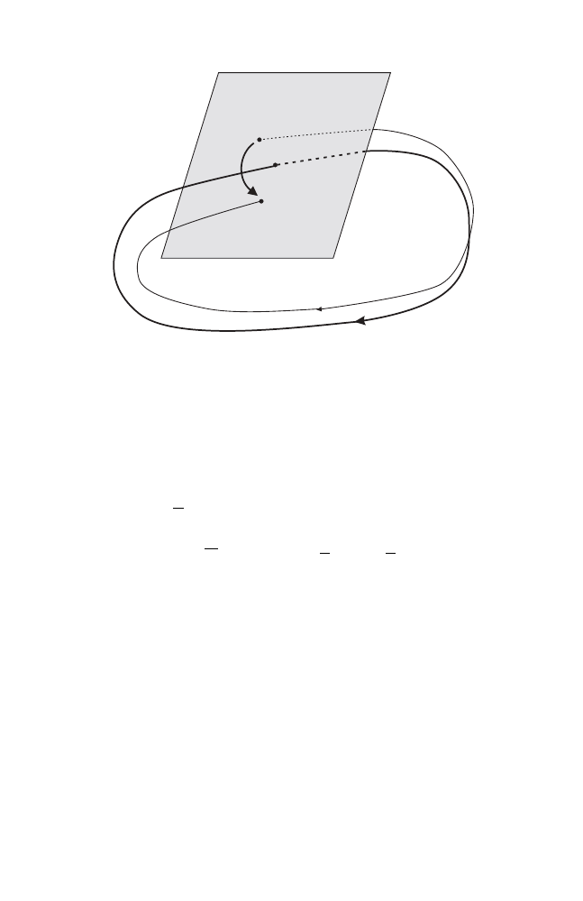
70
4 The minimal action near fixed points and invariant tori
g
p
W
Fig. 4.2. The Poincar´e map of a closed characteristic γ
In other words, the time is a generating function for the Poincar´
e return
map.
Proof. Let X be the Reeb flow, and denote its flow by ψ
t
. Consider the family
of mappings
f
t
(z) := ψ
tS(z)
(z).
Then f
1
= φ and
d
dt
f
t
(z) = S(z)X(f
t
(z)). Therefore
φ
∗
η
− η =
1
0
d
dt
f
∗
t
η dt =
1
0
f
∗
t
(i
d
dt
f
t
dη + di
d
dt
f
t
η) dt = dS
in view of (4.7).
The general question will be how much information about the geometry
of the contact manifold M is encoded in the closed characteristics. This is
the analogue of the question formulated and dealt with in Ch. 3 for convex
domains in the plane, where we asked how much information is hidden in the
length spectrum. In the setting of Reeb flows, however, the notion of length
has no meaning yet. Therefore we replace the length spectrum by the period
spectrum.
Definition 4.2.6. Let M be a 3–dimensional compact manifold. The period
spectrum
P(η) of a contact form η on M is defined as the set of periods of
all closed characteristics, together with all their (non–negative) multiples.

4.2 Contact flows in three dimensions
71
In the following, let us consider a continuous deformation η
s
, s
∈ [0, 1], of
contact forms on M such that each (M, η
s
) has the same period spectrum:
P(η
s
) =
P(η
0
)
for each s. How can the dynamics of the corresponding Reeb flows change
during the deformation?
4.2.1 Spectral invariants
Fran¸coise and Guillemin [32] conjectured that, in any odd dimension, such a
deformation preserving the period spectrum must be trivial, if it also fixes the
set of (symplectic conjugacy classes of) linearized Poincar´
e maps at the closed
characteristics. They proved that, if γ
s
is a nondegenerate elliptic closed char-
acteristic without resonances, the Birkhoff invariants of γ
s
stay fixed during
the deformation. This was generalized by Popov [87] who showed that the
Birkhoff invariants as well as the Liouville classes of invariant tori stay fixed,
even allowing resonances and dropping the condition that the deformation
preserves the linearized Poincar´
e maps.
What we will do is to show that, for the three–dimensional case, there is
a stronger invariant than just the Birkhoff normal form, namely the minimal
action. In order to apply the results from Sect. 4.1, we reduce the three–
dimensional Reeb flow to its two–dimensional Poincar´
e map near a closed
characteristic. For the latter, we assume that this reduction leads to a map
with a general elliptic fixed point (see Def. 4.1.9).
Definition 4.2.7. A closed trajectory γ of a three–dimensional Reeb flow is
called a general elliptic closed characteristic if the corresponding Poincar´
e
map φ has 0 as a general elliptic fixed point.
Note that this definition is independent of the choices of the point on
γ and the transverse section because two Poincar´
e maps are symplectically
conjugated and the conditions I.–IV. stated at the beginning of Sect. 4.1 are
invariant under such conjugations.
Then, applying the theory from Sect. 4.1, we can associate to a general
elliptic closed characteristic γ the half–sided germ of the minimal action α.
To be really consistent with our notation from the previous section where we
assumed that generating functions satisfy S(0) = 0, we replace the first return
time S(
·) by S(·) − T , where T is the (prime) period of γ; for simplicity, we
use the same letter S for the shifted first return time.
Now let η
s
, s
∈ [0, 1], be a continuous family of contact forms on M,
all having the same period spectrum, such that there is a continuous family
of general elliptic closed characteristics γ
s
. The next result states that the
corresponding minimal actions α
s
do not depend on s.

72
4 The minimal action near fixed points and invariant tori
Theorem 4.2.8. Suppose η
s
, s
∈ [0, 1], is a continuous deformation of contact
forms such that
P(η
s
) =
P(η
0
),
together with a continuous family of general elliptic closed characteristics γ
s
.
Then, as germs, we have
α
s
= α
0
for all s
∈ [0, 1].
Proof. Associated to each closed characteristic γ
s
, we have the half–sided
germ of the minimal action α
s
for the corresponding Poincar´
e return map.
Being continuous, each α
s
is uniquely defined by its values on
Q. We will
show below that, for a fixed rational rotation number p/q, the values α
s
(p/q)
vary continuously with s. Postponing the proof, we claim that these values
must be constant. Indeed, the period spectrum
P(η
s
), which is independent
of s by assumption, has Lebesgue measure 0 in
R. This follows from Sard’s
Theorem since closed characteristics correspond to critical points of a smooth
function. We had seen a similar argument in the proof of Prop. 3.2.2; for a
detailed proof see, for instance, [87, Prop. 3.2]. Therefore the values α
s
(p/q)
vary continuously in a set of measure zero, so they must stay fixed.
It remains to prove that α
s
(p/q) is continuous in s. For this, we recall from
Theorem 1.3.4 that for rational rotation numbers there is always a periodic
minimal orbit. Besides being periodic, these so–called Birkhoff orbits have
the additional property that they are ordered as if they were orbits of a rigid
rotation, and they can be found by minimizing the (discrete) action on the
compact space of ordered periodic sequences [51, Thm. 9.3.7]. As minima, the
corresponding minimal values α
s
(p/q) are indeed continuous in s.
In fact, one can even eliminate the assumption that we are given a family
of general elliptic closed characteristics. Its existence follows already from the
preservation of the period spectrum, as the next lemma shows; compare [87,
Lemma 3.5] for a similar argument.
In the general theory of dynamical systems, the eigenvalues of a linearized
Poincar´
e map Dφ(0) of some closed trajectory γ are called the Floquet mul-
tipliers of γ. .
Lemma 4.2.9. Suppose η
s
, s
∈ [0, 1], is a continuous deformation of contact
forms preserving the period spectrum, such that η
0
admits a general elliptic
closed characteristic γ
0
.
Then there is a continuous family of general elliptic closed characteristics
γ
s
for each η
s
, s
∈ [0, 1]. Moreover, their periods and Floquet multipliers do
not depend on s.
Proof. First of all, the condition that γ
0
is general guarantees that 1 is not a
Floquet multiplier of γ
0
. This implies that one can continue the fixed point
of the Poincar´
e map, corresponding to γ
0
, uniquely as a fixed point for small

4.2 Contact flows in three dimensions
73
s > 0, corresponding to a periodic trajectory γ
s
. This is a standard technique,
using the Implicit Function Theorem; see [98], for instance. Moreover, because
everything changes continuously with s, the new closed characteristics γ
s
are
general elliptic provided s is small enough, say, for s
∈ [0, δ). In addition,
since the period spectrum has Lebesgue measure 0, the periods of γ
s
are all
the same.
To each γ
s
we associate the germ of the minimal action α
s
. Thm. 4.2.8
implies
α
s
= α
0
.
It follows that the Birkhoff invariants of the Poincar´
e map, which are the
Taylor coefficients of α
∗
s
in view of Thm. 4.1.11, do not change along the
deformation. In particular, the Floquet multipliers stay fixed during the de-
formation. This proves the assertion for s
∈ [0, δ) where δ ∈ (0, 1] is assumed
to be maximal.
We want to show that δ = 1. Assume, on the contrary, that δ < 1. Then,
taking limits of the closed characteristics γ
s
as s
→ δ, we find a closed char-
acteristic for s = δ. Moreover, the Poincar´
e maps of γ
s
converge in the C
∞
–
topology to the Poincar´
e map of γ
δ
. Our assumption that the period spec-
trum remains unchanged implies that γ
δ
satisfies the conditions I.–III. from
Sect. 4.1. On the other hand, applying Thm. 4.1.11 again, we know that the
Birkhoff invariants of γ
δ
are the same as those of γ
0
. Thus, γ
δ
is again a gen-
eral elliptic closed characteristic. This proves that the set of parameters s, for
which there is a continuous family of general elliptic closed characteristics,
beginning with γ
0
, is open and closed in [0, 1]. Hence δ = 1, and the proof of
the lemma is finished.
Now we can translate our results for fixed points of symplectic mappings
into the language of contact geometry. Again, we point out that the minimal
action is a period spectrum invariant under continuous deformations of the
contact form.
Theorem 4.2.10. Suppose η
s
, s
∈ [0, 1], is a continuous family of contact
forms on a three–dimensional manifold with
P(η
s
) =
P(η
0
),
such that η
0
admits a general elliptic closed characteristic γ
0
.
Then there is a continuous family of general elliptic closed characteristics
γ
s
for s
∈ [0, 1] whose half–sided germs of minimal actions α
s
do not depend
on s:
α
s
= α
0
.
In particular, this implies the following:
1. The Birkhoff invariants of γ
0
and γ
1
are the same.
2. The Poincar´
e map φ
1
possesses an invariant circle of rotation number
p/q, consisting entirely of periodic orbits, if and only if φ
0
does.

74
4 The minimal action near fixed points and invariant tori
3. If φ
0
and φ
1
each have an invariant circle of rotation number ω, their
enclosed areas agree.
4. If φ
0
is integrable then φ
1
is C
0
–integrable.
Proof. Under the above assumptions, Lemma 4.2.9 implies that we have a
family of minimal actions α
s
which, by Thm. 4.2.8, are all equal. Thus, the
half–sided germ of the minimal action
α
s
= α
0
=: α
is a period spectrum invariant.
We prove the four implications. Since the Birkhoff invariants are the Taylor
coefficients of α
∗
(Thm. 4.1.11), they are invariant too. Moreover, φ
1
possesses
a periodic invariant circle of rotation number p/q if and only if α is differen-
tiable at p/q (Thm. 1.3.7); since α is invariant, the same holds true for φ
0
. A
similar argument proves the third statement because the area enclosed by an
invariant circle is given by α
(ω) (Thm. 1.3.7). Finally, if φ
0
is integrable then
α
∗
is an integrable Hamiltonian (Thm. 4.1.18); in particular, α is smooth,
which implies the C
0
–integrability of φ
1
.
4.2.2 Length spectrum invariants of surfaces
We consider a compact surface, i.e., a smooth compact two–dimensional Rie-
mannian manifold (M, g). As usual, the length spectrum
L(M, g)
is the set of lengths of all closed geodesics on M , together with all their
multiples. The question is how much information about the dynamics of the
geodesic flow is encoded in
L(M, g).
According to Ex. 4.2.4, the Hamiltonian vector field on the unit cotangent
bundle T
∗
1
M , conjugate to the geodesic vector field on the unit tangent bundle
T
1
M , is the Reeb vector field of the contact form
η := λ
|
T
∗
1
M
where λ is the canonical Liouville form on the cotangent bundle T
∗
M ; see
Ex. 2.1.14. Therefore, we may repeat the results from Sect. 4.2.1 for the case
of geodesic flows.
For this, we assume we have a continuous deformation g
s
, s
∈ [0, 1], of
Riemannian metrics on M starting at g
0
= g such that the length spectrum
is preserved:
L(M, g
s
) =
L(M, g
0
)
for all s
∈ [0, 1]. In addition, we suppose that g
0
possesses a general elliptic
closed geodesic γ
0
. Then, according to Lemma 4.2.9, there is a family of general

4.2 Contact flows in three dimensions
75
elliptic closed geodesics γ
s
for g
s
. Let us call α
s
the corresponding half–sided
germs of minimal actions. Thm. 4.2.10 implies that
α
s
= α
0
for all s
∈ [0, 1]. We may formulate a more pointed version of this as the
following principle.
Invariance Principle. Every quantity that can be calculated from the min-
imal action α is, by tautology, a length spectrum invariant under continuous
deformations of the Riemannian metric.
More precisely, we have the following result which is Thm. 4.2.10 applied
to the framework of Riemannian geometry.
Theorem 4.2.11. Suppose g
s
, s
∈ [0, 1], is a continuous family of Rieman-
nian metrics on a compact two–dimensional manifold that preserves the length
spectrum, such that g
0
admits a general elliptic closed geodesic γ
0
.
Then there is a continuous family of general elliptic closed geodesics γ
s
whose half–sided germs of minimal actions do not depend on s. In particular,
this implies the following:
1. The Birkhoff invariants of γ
0
and γ
1
are the same.
2. The Poincar´
e map φ
1
possesses an invariant circle of rotation number
p/q, consisting of periodic orbits, if and only if φ
0
does.
3. If φ
0
and φ
1
each have an invariant circle of rotation number ω, their
enclosed areas agree.
4. If the geodesic flow of g
0
is integrable near γ
0
then the geodesic flow of g
1
is C
0
–integrable near γ
1
.
Notice that an invariant circle of the Poincar´
e map gives rise to a two–
dimensional invariant torus of the geodesic flow around the closed geodesic;
see Fig. 4.3.
Remark 4.2.12. Concerning the last part of C
0
–integrability, there is the fol-
lowing unpublished result by G. Forni and S. Zelditch, announced in [103]; see
also [105]. Suppose you are given an analytic, rotationally symmetric metric
g on S
2
with certain additional nondegeneracy conditions. In this case, the
geodesic flow is integrable by Clairaut’s Theorem. Forni and Zelditch showed
that, if h is another metric with the same Laplace spectrum as g, the geodesic
flow of h is C
0
–integrable.
This remark leads to the question whether the Laplace spectrum charac-
terizes a manifold up to isometries. For instance, Kac’ question “Can one hear
the shape of a drum?” asked if there are non–isometric domains in the plane
with the same Laplace spectrum. It is well known that the answer is yes [35].
The Laplace spectrum is related to the length spectrum via trace formulae
76
4 The minimal action near fixed points and invariant tori
Fig. 4.3. Invariant tori of an integrable geodesic flow around a closed geodesic
and Poisson relations; we refer to [18, 38, 103] for details and more references.
Zelditch [104] showed that a special class of real analytic surfaces of revolution
is completely determined by the Laplace spectrum. The Birkhoff normal form
is still an essential ingredient for the proof but does not suffice to obtain the
full result.
4.3 The minimal action near positive definite invariant
tori
In this section, we formulate appropriate versions of the results of Sect. 4.1
for invariant tori of symplectic mappings in higher dimensions, rather than
for fixed points of area–preserving maps in the plane. The basic ideas are very
similar to those in Sect. 4.1.
Let (M, ω) be a 2n–dimensional symplectic manifold, and φ : M
→ M be
a smooth symplectic diffeomorphism; see Sect. 2.1.2 for definitions. Suppose
that Λ
⊂ M is an n–dimensional submanifold which is invariant under φ:
φ(Λ) = Λ.
Suppose further that φ
|
Λ
is smoothly conjugate to the translation on the
n–dimensional torus
T
n
by some vector ρ
∈ R
n
satisfying the Diophantine
condition
|k
0
+ k
· ρ| ≥ C |k|
−τ
(4.8)
for all k
0
∈ Z and k ∈ Z
n
\ {0}, where C and τ are some positive constants.
Under these assumptions, it follows from a remark by Herman [43] that
Λ is actually a Lagrangian submanifold of M . Therefore, by Weinstein’s La-
grangian neighbourhood theorem [73], there exists a neighbourhood of Λ in M

4.3 The minimal action near positive definite invariant tori
77
which is symplectically diffeomorphic to a neighbourhood of the zero section
in the cotangent bundle T
∗
Λ with its standard symplectic form. Note that Λ
is diffeomorphic to
T
n
and invariant under φ. Therefore, it follows that we
can find symplectic coordinates (x, y) in a neighbourhood of the zero section
T
n
× {0} in T
∗
T
n
=
T
n
× R
n
such that
φ(x, y) = (x + ρ + A(x)y, B(x)y) +
O(|y|
2
)
where A(x), B(x) are n
×n–matrices depending on the point x ∈ T
n
. Since the
standard symplectic form dy
∧ dx is preserved under the symplectic map φ,
B(x) is the identity matrix and A(x) is symmetric. Finally, the Diophantine
condition (4.8) guarantees that, by averaging A(x) over
T
n
, one can choose
symplectic coordinates in which the matrix A(x) becomes independent of x;
see [69] for details, or Thm. 4.3.6 for a refined version of this result.
Summarizing, under the above assumptions, there are symplectic coordi-
nates (x, y) near the zero section in T
∗
T
n
such that the map φ takes the
form
φ(x, y) = (x + ρ + Ay, y) +
O(|y|
2
)
(4.9)
where A is some n
× n–matrix.
In the end, we want to interpolate φ by a Hamiltonian, respectively La-
grangian, flow and apply Mather’s theory on minimizing measures. In order
to do so, we need some positive definiteness condition.
Definition 4.3.1. Let φ be a symplectic diffeomorphism with an invariant
torus Λ, such that there are symplectic coordinates near Λ in which (4.9)
holds. Then Λ is called positive definite if the matrix A in (4.9) is positive
definite.
Remark 4.3.2. It is actually sufficient to assume that A is just definite. For, if
A is negative definite, one considers φ
−1
instead of φ.
Remark 4.3.3. The positive definiteness of Λ is a well defined notion. Indeed,
if we choose different coordinates (x
, y
) leading to a representation
φ(x
, y
) = (x
+ ρ + A
y
, y
) +
O(|y
|
2
)
with a different symmetric matrix A
then one can calculate that A
= B
AB
where B is some invertible matrix. Hence A
is positive definite if, and only
if, A is.
The following elementary lemma shows that the locally defined symplectic
diffeomorphism φ can be embedded in a global Hamiltonian flow on T
∗
T
n
gen-
erated by a convex Hamiltonian. Therefore, it fits into the setting of Mather–
Ma˜
n´
e theory.
Lemma 4.3.4 ([69]). Let Λ be a positive definite invariant torus of a sym-
plectic diffeomorphism φ defined in a neighbourhood of Λ. Then φ can be
written as the restriction of the time–1–map of a Hamiltonian flow on T
∗
T
n
generated by a convex Hamiltonian on
S
1
× T
∗
T
n
.

78
4 The minimal action near fixed points and invariant tori
Applying Mather–Ma˜
n´
e theory to the extended convex Hamiltonian, re-
spectively Lagrangian, yields the corresponding minimal action defined on
H
1
(
T
n
,
R). A priori, this function depends on the extension of φ and the
choice of interpolating Lagrangian.
Concerning the dependence on the Lagrangian, Mather showed [67, 69]
that there is a one–to–one correspondence between invariant measures of L
and invariant measures of its time–1–map, and that the choice of a different
interpolating Lagrangian affects the minimal action only by an affine function
of the rotation vector. Let us identify H
1
(
T
n
,
R) = R
n
in such a way that
the homological rotation vector of the unique invariant measure supported on
T
n
× {0} is mapped onto ρ. Then, up to irrelevant additive constants, the
minimal action does not depend on the interpolating Lagrangian anymore.
The dependence on the extension is more crucial. It follows from the a
priori bound on the Lipschitz constant in Thm. 2.1.11, however, that minimal
invariant measures of rotation vectors near ρ (the rotation vector of the in-
variant torus Λ) lie also near Λ; see [69]. This localization result implies that
the germ of the minimal action at ρ does not depend on the extension of φ.
Summarizing, we have the following result.
Proposition 4.3.5 ([69, 8]). Associated to the germ of a symplectic diffeo-
morphism at a positive definite invariant torus with rotation vector ρ, there
is the germ of the corresponding minimal action at ρ, which is a symplectic
invariant.
In the following, we want to show that the germ of the minimal action
contains the Birkhoff invariants of the invariant torus, just as we did in
Thm. 4.1.11 for the setting of a fixed point. The Birkhoff normal form of
a symplectic diffeomorphism near an invariant torus is described in the fol-
lowing classical result; compare [26, App. 2] or [55, Prop. 9.13].
Theorem 4.3.6 (Birkhoff normal form). Let Λ be a positive definite in-
variant torus of a symplectic diffeomorphism φ such that φ
|
Λ
is conjugate to
the translation by a vector ρ satisfying the Diophantine condition (4.8).
Then, for each N
≥ 2, there is a symplectic change of coordinates trans-
forming φ into the form
φ(x, y) = (x +
∇P
N
(y), y) +
O(|y|
N
)
(4.10)
as y
→ 0 where P
N
is a polynomial of degree N . The coefficients of P
N
are
called the Birkhoff invariants of φ; they are symplectically invariant.
Note that, according to (4.9), one has
P
N
(y) = ρ
· y +
1
2
Ay
· y + O(|y|
3
)
if one ignores irrelevant additive constants.

4.3 The minimal action near positive definite invariant tori
79
Analogously to Sect. 4.1, we will show that the minimal action near an
invariant torus comprises its Birkhoff invariants. This result was also proven
by Bernard [8], with a slightly different approach.
Theorem 4.3.7. Let Λ be a positive definite invariant torus of a symplectic
diffeomorphism φ such that φ
|
Λ
is conjugate to the translation on
T
n
by a
vector ρ satisfying the Diophantine condition (4.8).
Then the germ of the corresponding minimal action α at ρ is a symplectic
invariant. Moreover, the Birkhoff invariants of φ are the Taylor coefficients
of α
∗
at 0.
Proof. In view of Thm. 4.3.6, we can assume that φ is already given in the
form
φ(x, y) = (x +
∇P
N
(y), y) +
O(|y|
N
)
(4.11)
for any given N
≥ 2. Let us denote by
φ
0
(x, y) := (x +
∇P
N
(y), y)
the integrable part, i.e., the Birkhoff normal form, of φ. Then φ
0
can be written
as the time–1–map of the flow of the integrable Hamiltonian
H
0
(x, y) := ρ
· y +
1
2
Ay
· y + O(|y|
3
) = P
N
(y).
Since A is assumed to be positive definite, the Hamiltonian H
0
: T
∗
T
n
→ R
is convex and possesses a corresponding convex Lagrangian L
0
: T
T
n
→ R
which is the convex conjugate P
∗
N
of the polynomial P
N
. A quick calculation
shows that
L
0
(x, p) =
1
2
A
−1
(p
− ρ) · (p − ρ).
(4.12)
Up to now, everything was defined only in a neighbourhood of the invari-
ant torus Λ. Lemma 4.3.4, however, allows us to extend the map and the con-
vex Hamiltonian to the whole cotangent bundle T
∗
T
n
. Moreover, Prop. 4.3.5
guarantees that the germ of the minimal action corresponding to the extended
convex Hamiltonian, respectively Lagrangian, is a symplectic invariant which
is independent of the extension. Therefore, thinking in terms of germs now,
the minimal action α
0
corresponding to the integrable Lagrangian L
0
is given
by
α
0
= L
0
= P
∗
N
(4.13)
where we identified H
1
(
T
n
,
R) = R
n
as above.
Next, we want to show a continuity property of the minimal action with
respect to the Lagrangian, similar to Prop. 1.3.8 for the two–dimensional case.
For this, we make use of the following characterization of the convex conjugate
of the minimal action by Ma˜
n´
e’s critical value, given in Cor. 2.2.6. Namely,
we have
α
∗
([ν]) = c(L
− ν)

80
4 The minimal action near fixed points and invariant tori
for every closed 1–form on
T
n
, where the critical value c(L) is defined in
Def. 2.2.1. The main point is that the critical value c(L) is monotone in the
Lagrangian, i.e., if two Lagrangians satisfy the pointwise inequality L
1
≤
L
2
then c(L
1
)
≥ c(L
2
); this can be seen most easily by looking at (2.8).
Reformulated for the minimal action, we conclude that
L
1
≤ L
2
=
⇒ α
∗
L
1
≥ α
∗
L
2
⇐⇒ α
L
1
≤ α
L
2
.
Having proven the monotonicity of the minimal action with respect to the
Lagrangian, it follows from (4.11) and (4.13) that
α(h) = α
0
(h) +
O(|h|
N
) = P
∗
N
(h) +
O(|h|
N
).
Since the coefficients of P
N
are the Birkhoff invariants of φ, the theorem is
proven.

5
The minimal action and Hofer’s geometry
The classical dynamical way of investigating Hamiltonian systems is to look at
one single system at a time. The development of symplectic topology changed
this and added a more geometric point of view. Namely, for a given symplectic
manifold (M, ω) one has the infinite–dimensional Lie group Ham(M, ω) of all
Hamiltonian diffeomorphisms. It was an astonishing discovery by Hofer in
1990 [44], later extended by Lalonde and McDuff [53], that this group comes
equipped with an intrinsic geometry given by a bi–invariant Finsler metric.
This opened the field of studying the geometry, and even the topology, of
Ham(M, ω) both of which are sometimes a bit mysterious.
On the other hand, definite progress has been made: geodesics in Hofer’s
geometry are completely understood [12], the existence of minimal geodesics
has been established in some situations [45, 54, 92]—there are even purely
symplectic bounds for the first eigenvalue of the Laplacian [83]. The methods
that enter into the proofs are manifold: they range from dynamical systems
over symplectic geometry to algebraic geometry. For recent developments in
the study of the geometry of Hamiltonian diffeomorphism groups we refer to
[46, 54, 82, 84, 85].
The motivation for the subsequent work was to find connections between
the two branches in Hamiltonian mechanics mentioned above, the classical dy-
namical and the modern geometric one. In a sense, the geometric viewpoint
seems simpler—the full dynamical system is being described by one Hamilto-
nian function and corresponds to one path in the Hamiltonian diffeomorphism
group. The central problem is to deduce dynamical properties of the system
from geometric properties of the path.
A distinguished class of Hamiltonian systems is rooted in classical me-
chanics. These are mechanical systems where the Hamiltonian is composed of
two parts: kinetic energy plus potential energy. An essential feature of such
systems is that they satisfy the Legendre condition which allows to switch
between Hamiltonian and Lagrangian mechanics.
The main result of this chapter describes a relation between Hofer’s ge-
ometry and Mather’s theory of minimal action. We will see that minimizing
K.F. Siburg: LNM 1844, pp. 81–95, 2004.
c
Springer-Verlag Berlin Heidelberg 2004

82
5 The minimal action and Hofer’s geometry
measures play an important role, for the dynamics as well as for the geometry
of a Hamiltonian system.
5.1 Hofer’s geometry of Ham(
M, ω)
Consider a Hamiltonian flow on a symplectic manifold. In classical mechanics,
for instance, the flow of a Hamiltonian of the form H(x, y) = 1/2
|y|
2
− V (x),
where V is some smooth potential, describes the motion of a particle in the
potential V ; compare Ex. 1.1.7. The value of the Hamiltonian, the energy, is
constant along the trajectories; in the case indicated above, it is the sum of
kinetic and potential energy.
Instead of following a trajectory continuously, we might also consider a
“stroboscopic” picture of it, by looking at it only at discrete times, e.g., at all
integer times. From the dynamical systems point of view, this means that we
consider the time–1–map rather than the flow. In the case of a Hamiltonian
flow, the time–1–map is a Hamiltonian diffeomorphism. Given a Hamiltonian
diffeomorphism, one might ask the following “economical” question. Is it pos-
sible to generate the given map by a Hamiltonian flow with less energy?
This idea will eventually lead to a bi–invariant metric on the group of
Hamiltonian diffeomorphisms, the so–called Hofer metric, which is one of the
cornerstones of modern symplectic topology. The resulting geometry is called
Hofer’s geometry. Its geometric features, and its connection to dynamics, seem
somewhat strange and are being studied quite intensively.
Let us, first of all, define Hofer’s metric and deduce some simple properties.
For a detailed exposition we refer to [46, 85]. Let (M, ω) be a symplectic man-
ifold, i.e., a 2n–dimensional manifold M with a closed, nondegenerate 2–form
ω; compare Sect. 2.1.2. A Hamiltonian diffeomorphism is a diffeomorphism
φ : M
→ M which can be written as the time–1–map of a Hamiltonian flow,
i.e.,
φ = ϕ
1
H
for some time–periodic Hamiltonian H :
S
1
×M → R. Let us denote by H
t
the
function H(t,
·) on M. In the following, we will normalize the Hamiltonians,
so that the ambiguity of adding constants is removed.
Definition 5.1.1. Let (M, ω) be a symplectic manifold without boundary. If
M is open, the set of admissible Hamiltonians is defined as
H := {H : S
1
× M → R | supp H
t
is compact for every t
},
where supp denotes the support of a function. If M is compact, we set
H := {H : S
1
× M → R |
M
H
t
dω
n
= 0 for every t
}.
In any case, the group of Hamiltonian diffeomorphisms of a symplectic
manifold (M, ω) is given by

5.1 Hofer’s geometry of Ham(
M, ω)
83
Ham(M, ω) :=
{φ : M → M | φ = ϕ
1
H
for some H
∈ H}.
A Hamiltonian H :
S
1
× M → R defines a path t → ϕ
t
H
in the diffeomor-
phism group Ham(M, ω). We measure the length of this path by
(H) :=
S
1
osc H
t
dt
where osc := max
− min denotes the oscillation of a function on M. For H ∈
H, it is clear that (H) = 0 if, and only if, H = 0. Like in the case of Finsler
geometry we measure the distance from the identity in Ham(M, ω) by taking
the infimum of lengths of all connecting paths.
Definition 5.1.2. The distance from the identity, or energy, of an element
φ
∈ Ham(M, ω) is defined as
d(id, φ) := inf
{(H) | H ∈ H such that φ = ϕ
1
H
}.
Remark 5.1.3. Note that (H) measures the C
0
–data of the Hamiltonian (cor-
responding to the energy) and not the C
1
–data (which define the flow). There-
fore, d(id, φ) indeed describes the minimal amount of energy necessary to
generate a given map φ. On the other hand, it seems that d measures the
“wrong” kind of data, at least from the dynamical systems viewpoint. Eliash-
berg and Polterovich [27]proved, however, that this is the only way of defining
a bi–invariant metric.
Let us extend the distance to a bi–invariant function d : Ham(M, ω)
×
Ham(M, ω)
→ [0, ∞) by setting
d(φ, ψ) := d(id, ψ
◦ φ
−1
).
It follows quite easily from the definition of d and the transformation law
of Hamiltonian vector fields that d defines a bi–invariant pseudo–metric on
Ham(M, ω), i.e., a function with
d(φ
◦ χ, ψ ◦ χ) = d(χ ◦ φ, χ ◦ ψ) = d(φ, ψ)
that satisfies all the axioms of a metric, except that it might be degenerate.
It is not clear at all whether d(id, φ) = 0 should imply φ = id; compare
Rem. 5.1.3. It was Hofer [44] who discovered that the pseudo–distance d is
actually a genuine metric.
Theorem 5.1.4 (Hofer). The pseudo–metric d is nondegenerate and, there-
fore, a bi–invariant metric on the Hamiltonian diffeomorphism group
Ham(M, ω).
This metric is called Hofer’s metric. It is intrinsically defined, i.e., via the
lengths of paths inside the group itself. Consequently, it defines a Finsler geom-
etry on Ham(M, ω). Of particular importance are globally length–minimizing
paths.
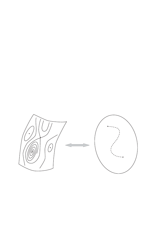
84
5 The minimal action and Hofer’s geometry
Definition 5.1.5. Let (M, ω) be a symplectic manifold and H
∈ H an admis-
sible Hamiltonian. Then H is said to generate a minimal geodesic if
d(id, ϕ
1
H
) = (H).
Hofer’s geometry allows also the notions of geodesics, conjugate points,
etc. We refer to [12, 54, 84, 85, 92] for further definitions and results.
We want to pursue the following idea here. A Hamiltonian dynamical sys-
tem corresponds to one single path in the Hamiltonian diffeomorphism group,
and vice versa. Therefore, this path contains all information about the Hamil-
tonian dynamical system (like periodic orbits, heteroclinic connections, etc.).
The group Ham(M, ω), on the other hand, is equipped with a geometry com-
ing from Hofer’s metric, and the path has certain properties with respect
to this geometry (like being a geodesic, etc.). What kind of relations exist
between the (finite–dimensional) dynamics of the Hamiltonian flow and the
(infinite–dimensional) Hofer geometry of the corresponding path? In particu-
lar, what kind of information about Hofer’s geometry can be retrieved from
the classical dynamics? Take a look at Fig. 5.1 to see the two viewpoints of a
Hamiltonian system, the dynamical and the geometric one.
M
Ham(M, )
w
id
f
d y n a m i c a l
g e o m e t r i c
Fig. 5.1. Two viewpoints of a Hamiltonian system
In the following, we go back to the phase space of classical mechanics
and consider the cotangent bundle T
∗
T
n
with its canonical symplectic form
ω
0
= dλ. In order to include Hamiltonians satisfying the Legendre condition
(see Sect. 2.1.1) into the framework of Hofer’s geometry, we have to restrict
them to a compact part of T
∗
T
n
; otherwise, they would violate the compact

5.1 Hofer’s geometry of Ham(
M, ω)
85
support condition. Denote by
B
∗
T
n
:=
T
n
× {|y| ≤ 1}
the unit ball cotangent bundle of the torus. We also restrict the class of ad-
missible Hamiltonians and consider the set
H
0
consisting of all smooth Hamil-
tonians H :
S
1
× B
∗
T
n
→ R that satisfy the following two conditions:
1. H :
S
1
× B
∗
T
n
→ R vanishes on the boundary of B
∗
T
n
, i.e., H(
·, ·, y) = 0
whenever
|y| = 1;
2. H :
S
1
× B
∗
T
n
→ R admits a smooth extension
H :
S
1
× T
∗
T
n
→ R
which is only a function of t and
|y|
2
outside
S
1
× B
∗
T
n
.
As before, we consider the group
Ham(B
∗
T
n
) :=
{φ : B
∗
T
n
→ B
∗
T
n
| φ = ϕ
1
H
for some H
∈ H
0
}
of Hamiltonian diffeomorphisms generated by Hamiltonians in
H
0
.
In order to prove estimates for d(id, φ) when φ is generated by a convex
Hamiltonian H
∈ H
0
, we need the following notion. As usual, ϕ
H
denotes the
flow corresponding to a Hamiltonian function H.
Definition 5.1.6. Given any H
∈ H
0
, the set
σ
c
(H) :=
Γ
λ
− Hdt | Γ contractible 1–periodic orbit of ϕ
H
is called the contractible action spectrum of H.
Note that
λ
−Hdt corresponds to the action integral
L dt. Thus, σ
c
(H)
collects the actions of all 1–periodic trajectories of the Hamiltonian flow that
belong to contractible orbits. Hofer proved [45] that this set plays a crucial
role in the geometry of the Hamiltonian diffeomorphism group Ham(
R
2n
, ω
0
).
We will see here that the smallest action of a contractible orbit yields a lower
bound for the energy of a map which is generated by a convex Hamilto-
nian. The following theorem is a slight generalization of a result by Bialy and
Polterovich [12, Prop. 4.3.A].
Theorem 5.1.7. Suppose φ
∈ Ham(B
∗
T
n
) is generated by a convex Hamil-
tonian H
∈ H
0
. Then
d(id, φ)
≥ inf σ
c
(H) > 0.
Proof. The first, main step is to show that
d(id, φ)
≥ inf σ
c
(H).
(5.1)
86
5 The minimal action and Hofer’s geometry
The second step will be to prove that
inf σ
c
(H) > 0.
(5.2)
For the first inequality we could essentially use a proof of Hofer and Zehn-
der [46] if φ was defined on all of T
∗
T
n
and had compact support. So we will
build an appropriate “nice” extension
φ : T
∗
T
n
→ T
∗
T
n
of φ : B
∗
T
n
→ B
∗
T
n
, and find a procedure how to extend any given K
∈ H
0
with ϕ
1
K
= φ to a Hamiltonian on
S
1
× T
∗
T
n
whose time–1–map coincides
with φ.
Let us fix, once and for all, some > 0. We define the map φ in the
following way. By definition of
H
0
, there is an extension
H :
S
1
× T
∗
T
n
→ R
of H :
S
1
× B
∗
T
n
→ R which is a function of t and |y|
2
for
|y| ≥ 1. Since H
is convex and satisfies the boundary condition H = 0 on
{|y| = 1}, we have
H
≤ 0. This implies that the derivative H
t
(1), seen as a function of
|y|
2
, is
positive. Therefore, we can pick an extension H with the following properties:
1. H
t
> 0 for 1
≤ |y| < 2
2. 0
≤ H ≤ for |y| ≥ 1
3. H = for
|y| ≥ 2.
Note that for
|y(0)| ≥ 1 the time–t–map ϕ
t
H
(x(0), y(0)) = (x(t), y(t)) is given
by
x(t)
= x(0) + y(0)
t
0
H
s
(
|y(0)|
2
) ds
y(t)
= y(0)
(5.3)
In other words, outside B
∗
T
n
, the flow of H at time t is just the geodesic flow
at time
t
0
H
s
ds. Let us call
φ := ϕ
1
H
.
Given any (not necessarily convex) K
∈ H
0
with ϕ
1
K
= φ, we claim that
we can extend K to a smooth function K :
S
1
× T
∗
T
n
→ R such that
1. K is a function of t and
|y|
2
for
|y| ≥ 1
2. 0
≤ K ≤ 3 for |y| ≥ 1
3. K = for
|y| ≥ 2
4. ϕ
1
K
= ϕ.
Of course, only the last point has to be checked. For that we pick any extension
K satisfying the first three conditions with 0
≤
K
≤ for |y| ≥ 1, and define
K(t, x, y) :=
K
t
(
|y|
2
) +
S
1
(H
t
(
|y|
2
)
−
K
t
(
|y|
2
)) dt
if
|y| ≥ 1
K(t, x, y)
if
|y| ≤ 1

5.1 Hofer’s geometry of Ham(
M, ω)
87
By (5.3), K fulfills all four requirements provided it is smooth, which can be
seen as follows. The smooth diffeomorphisms ϕ
1
K
and ϕ
1
H
coincide on
{|y| ≤
1
}, hence all their derivatives at points on {|y| = 1} are the same. Therefore,
S
1
(H
t
(
|y|
2
)
−
K
t
(
|y|
2
)) dt is a smooth function on
{|y| ≥ 1} that vanishes
with all its derivatives on
{|y| = 1}. Thus, K is the extension we were looking
for.
We are going to prove (5.1). The flow of the extended Hamiltonian H :
S
1
× T
∗
T
n
→ R has no (non–constant) contractible 1–periodic orbits outside
B
∗
T
n
. We eliminate all non–contractible 1-periodic orbits of ϕ
H
by choosing
an appropriate covering of
T
n
. Moreover, we can embed the compact part
of T
∗
T
n
with
|y| ≤ 2 symplectically into R
2n
and view φ = ϕ
1
H
as being
generated by the compactly supported Hamiltonian H
− : S
1
× R
2n
→
(
−∞, 0]. For the contractible action spectrum we have
σ
c
(H
− ) = (σ
c
(H) + )
∪ {0}.
Let us call d
0
the usual Hofer metric on the group Ham(
R
2n
, ω
0
) of Hamil-
tonian diffeomorphisms generated by compactly supported Hamiltonians on
S
1
× R
2n
. In this, setting, Hofer and Zehnder proved that the inequality
d
0
(id, φ)
≥ inf σ
c
(H) +
(5.4)
holds; see [46, Ch. 5] for details. Now we pick any K
∈ H
0
such that ϕ
1
K
= φ
and
d(id, φ)
≥
S
1
osc K
t
dt
− .
As described above, we can extend K to K with ϕ
1
K
= φ and
S
1
osc K
t
dt
≥
S
1
osc K
t
dt
− 6,
so that we can estimate
d(id, φ)
≥
S
1
osc K
t
dt
− 7.
(5.5)
We point out here that non–contractible periodic orbits of ϕ
K
and ϕ
H
are homotopic with fixed end points because ϕ
1
K
= ϕ
1
H
. Thus, the covering
needed to eliminate those orbits does not depend on the particular choice of
Hamiltonian generating φ.
From (5.4) we conclude that
S
1
osc K
t
dt
≥ d
0
(id, φ)
≥ inf σ
c
(H) +
which, together with (5.5), finally implies that

88
5 The minimal action and Hofer’s geometry
d(id, φ)
≥ inf σ
c
(H)
− 6.
Since > 0 was arbitrarily small, this finishes the proof of (5.1).
As the final step, we have to show that the contractible action spectrum
σ
c
(H) consists of positive numbers. This is already done in [12] and repeated
here for the convenience of the reader. Pick any contractible 1–periodic orbit
Γ = (x(t), y(t))
0≤t≤1
, and let Λ = gr ν be a Lagrangian section in B
∗
T
n
(ν
is a closed 1–form on
T
n
). It follows that
Γ
λ
− Hdt =
Γ
λ
− π
∗
ν
− Hdt
=
S
1
(y
− ν) ∂
y
H
− H
dt
≥
S
1
−H(t, x(t), ν(x(t))) dt
by the convexity of H
≥
S
1
min(
−H(t, ·)|
Λ
) dt.
The convexity of H, in conjunction with the zero boundary condition, implies
that H
≤ 0. Therefore, we have
S
1
min(
−H(t, ·)|
Λ
) dt > 0
and, hence, inf σ
c
(H) > 0.
This proves (5.2) and completes the proof of Thm. 5.1.7.
Remark 5.1.8. Thm. 5.1.7 holds also true if we replace the flat norm
| · | by
| · |
g
where g is any Riemannian metric on
T
n
without contractible closed
geodesics.
Remark 5.1.9. Iturriaga and S´
anchez–Morgado generalized Thm. 5.1.7 to gen-
eral cotangent bundles; see [48].
The action spectrum of an arbitrary convex Hamiltonian H defies compu-
tation. If we restrict ourselves to integrable Hamiltonians H = H(t, y), how-
ever, the only contractible periodic solutions are constant. Therefore, σ
c
(H)
consists of all values
−
S
1
H
t
(y
0
) dt where y
0
is a critical point of H
t
for all
t. Thm. 5.1.7 then states that
d(id, ϕ
1
H
)
≥ min
y
0
−
S
1
H
t
(y
0
) dt
where y
0
is as above. Note that, in this inequality, the left hand side involves
all Hamiltonians generating the map ϕ
1
H
, not just the convex ones.
In fact, we can give a characterization of those integrable convex Hamil-
tonians that generate a minimal geodesic.

5.2 Estimates via the minimal action
89
Theorem 5.1.10. Let H = H(t, y) be an integrable convex Hamiltonian in
H
0
. Then H generates a minimal geodesic if, and only if, all H
t
attain their
minimum at one and the same point y
min
.
Proof. Suppose H(t, y) is convex and has a fixed minimal point y
min
. Then
K(y) :=
S
1
H(t, y) dt
∈ H
0
is convex, generates the same time–1–map as H, and has the same energy:
(K) =
S
1
osc K
t
dt =
−K(y
min
) =
S
1
osc H
t
dt = (H).
But then σ
c
(K) =
{−K(y
min
)
} implies, by Theorem 5.1.7, that K generates
a minimal geodesic. Since (K) = (H), H generates a minimal geodesic, too.
Conversely, the existence of a fixed minimal point is necessary for a Hamil-
tonian H
∈ H
0
in order to generate a minimal geodesic. This is proven in [54,
Prop. 2.1]. In fact, if H does not have a fixed minimal point then there exists
a strictly shorter connection between the identity and ϕ
1
H
.
Remark 5.1.11. In the case of Ham(
R
2n
, ω
0
), a Hamiltonian with (isolated)
fixed minimal and maximal points generates a minimal geodesic as long as
it does not generate non–constant closed orbits; see [92]. The proof involves
perturbations of the Hamiltonian near the fixed minimal and maximal points.
Since this is only local, a generalized version of Thm. 5.1.10 should hold for
non–integrable convex Hamiltonians.
In particular, Thm. 5.1.10 states that every time–independent, convex, in-
tegrable Hamiltonian describes a minimal geodesic. This implies the following
result.
Corollary 5.1.12. The diameter of (Ham(B
∗
T
n
), d) is infinite.
5.2 Estimates via the minimal action
Consider a convex Hamiltonian H :
S
1
× B
∗
T
n
→ R in H
0
, and extend it by
some function of t and
|y|
2
to a convex Hamiltonian H :
S
1
× T
∗
T
n
→ R.
Associated to this extension we have the minimal action
α := α
H
: H
1
(
T
n
,
R) → R.
Our aim in this section is to relate the function α to the Hofer distance d(id, φ)
of the time–1–map φ := ϕ
1
H
on B
∗
T
n
.
The idea why this should be possible at all is prompted by the following
observation. Suppose for a moment that H = H
0
(y) is integrable and convex.
Then Thm. 5.1.10 states that H
0
generates a minimal geodesic:

90
5 The minimal action and Hofer’s geometry
d(id, φ) = osc H
0
.
On the other hand, we know from Cor. 2.1.25 that α
∗
= H
0
if we identify
H
1
(
T
n
,
R
n
) =
R
n
. Hence we obtain
d(id, φ) = osc
B
∗
T
n
H
0
= osc
B
α
∗
(5.6)
where the oscillation of α
∗
is taken over the unit ball B
⊂ R
n
. Thus, if we view
α
∗
|
B
as an integrable Hamiltonian on B
∗
T
n
, it generates a minimal geodesic
in Ham(B
∗
T
n
)!
Since α
∗
= 0 on the boundary of the unit ball B, we have osc α
∗
=
− min α
∗
, which is nothing but α(0) by (2.4), so that we may rewrite (5.6) as
d(id, φ) = α(0).
(5.7)
Unfortunately, already the simplest non–integrable example will show that
(5.6), respectively (5.7), does not hold in general.
Example 5.2.1. Consider the Lagrangian
L(x, p) =
p
2
2
− V (x)
of a particle in a periodic potential in one degree of freedom, e.g., the motion
of a mathematical pendulum. We assume that V attains its minimum at x = 0
with V (0) = 0. Of course, the corresponding Hamiltonian
H(x, y) =
y
2
2
+ V (x)
does not belong to
H
0
because it does not satisfy the boundary conditions.
Therefore we fix a cut off function β : [0, 1]
→ [0, 1] with β(s) = 1 if s ≤ 1/2,
and consider the modified Hamiltonian
H(x, y) :=
1
2
(y
2
− 1) + β(y
2
)V (x).
If max V is sufficiently small, H is a convex function and does belong to
H
0
.
Moreover, we assume that the outer separatrices, defined by H =
−1/2 +
max V , lie in the region
{y
2
≤ 1/2} where β plays no role anymore. Then
these separatrices are the graphs
y(x) =
±
2(max V
− V (x)),
and the region between them is filled by fixed points, periodic orbits, and
maybe also further separatrices; see Fig. 5.2.
What is the value α(0) of the minimal action in this example? Setting
p = 0 and x = x
max
such that V (x
max
) = max V , we see that a minimal
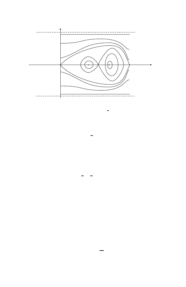
5.2 Estimates via the minimal action
91
y
x
x
+1
max
x
max
1
-1
Fig. 5.2. The level sets of H(x, y) =
1
2
(
y
2
− 1) + β(y
2
)
V (x)
measure of zero rotation vector is concentrated on the fixed point (x
max
, 0),
and hence we have
α(0) =
1
2
− max V.
(5.8)
This means that α does not “see” the entire region between the outer sepa-
ratrices.
Observe now that a C
2
-small potential V will admit only non–constant
periodic orbits of period greater than one. Therefore, by a criterion due to
Hofer [45, 92], H generates a minimal geodesic, so that
d(id, φ) =
1
2
>
1
2
− max V = α(0),
(5.9)
and (5.7) does indeed not hold.
We saw that the distance from the identity of the time–1–map of a convex
Hamiltonian can be smaller than α(0). But what happens if we do not restrict
the time to being at most 1 but let it tend to infinity? In fact, from the
geometric point of view, the time t = 1 is not distinguished at all. If we
consider a path in Ham(M, ω), a more relevant piece of information would be
the average distance from the identity over all times. This idea leads to the
following notion.
Definition 5.2.2. The asymptotic distance from the identity of an element
φ
∈ Ham(M, ω) is defined as
d
∞
(id, φ) := lim
N
→∞
1
N
d(id, φ
N
).

92
5 The minimal action and Hofer’s geometry
Remark 5.2.3. It follows from the triangle inequality that d
∞
≤ d. Hence the
limit in Def. 5.2.2 always exists. Moreover, lower estimates for the asymptotic
distance d
∞
are stronger than the same estimates for the distance d.
The asymptotic distance was introduced by Bialy and Polterovich [13]. It
measures the deviation of a path from being a minimal geodesic. Note that, in
general, minimal geodesics will eventually lose the property of being shortest
connections.
In the following, we will give an estimate of the asymptotic distance of a
convex Hamiltonian H by α(0) where α is the minimal action for some convex
extension of H. To do so, we must first show that the value α(0) does not
depend on the particular extension.
Let H :
S
1
× B
∗
T
n
→ R be a convex Hamiltonian in H
0
. Consider any
convex extension H :
S
1
×T
∗
T
n
→ R of H that is a function t and |y|
2
outside
B
∗
T
n
, and let α
H
: H
1
(
T
n
,
R) → R be the corresponding minimal action.
Lemma 5.2.4. The value α
H
(0) is independent of the particular extension
H.
Proof. We identify H
1
(
T
n
,
R) = R
n
in such a way that [λ
|
T
n
×{y}
] = y. Note
that, for
|y| ≥ 1, the torus T
n
× {y} is invariant under each ϕ
t
H
which is a
fixed rotation there. Cor. 2.1.25 implies that
α
∗
H
(y) =
1
0
H
t,
1
2
|y|
2
dt
for
|y| ≥ 1; in particular, α
∗
H
(y) = 0 whenever
|y| = 1. Since α
∗
H
is convex it
must attain its negative minimum in the unit ball where H = H. Therefore,
− min α
∗
H
= α
H
(0) does not depend on the choice of extension of H.
In view of Lemma 5.2.4 we may ignore the particular choice of extension,
and drop the index H. We state the main result of this section.
Theorem 5.2.5. Suppose φ
∈ Ham(B
∗
T
n
) is generated by a convex Hamil-
tonian. Then
d
∞
(id, φ)
≥ osc α
∗
= α(0).
Proof. Fix any convex H
∈ H
0
such that ϕ
1
H
= φ. Recall from Thm. 5.1.7
that
d(id, φ)
≥ inf σ
c
(H)
where σ
c
(H) is the contractible action spectrum of H. Each contractible 1–
periodic orbit is the support of an invariant probability measure with rotation
vector zero. Hence
inf σ
c
(H)
≥ α(0)
with α(0) =
− min α
∗
= osc α
∗
.
This proves that d(id, φ)
≥ α(0). The theorem follows by observing that
α(N h, φ
N
) = N α(h, φ).

5.2 Estimates via the minimal action
93
Remark 5.2.6. Bialy and Polterovich proved in [12, Thm. 1.4.A] that the Hofer
distance is bounded from below by the quantity
C
H
= sup
Λ
S
1
min(
−H
t
|
Λ
) dt > 0
where Λ runs over all Lagrangian sections in B
∗
T
n
. In general, the dynamical
meaning of C
H
is not quite clear. For autonomous Hamiltonians, however,
this number agrees with our lower bound since
C
H
=
− inf
c
∈H
1
inf
[ν]=c
max H(x, ν(x)) =
− inf
c
∈H
1
α
∗
(c) = α(0),
where the second last equality follows from Cor. 2.2.6 and (2.9).
Remark 5.2.7. The first nontrivial class of examples where d
∞
could actually
be calculated is given by compactly supported autonomous Hamiltonians on
a surface of infinite area; see [86].
Remark 5.2.8. Iturriaga and S´
anchez–Morgado [48] gave a generalized version
of Thm. 5.2.5 and proved the estimate d(id, φ)
≥ α(0) for convex Hamiltonians
on general cotangent bundles.
Let us continue Ex. 5.2.1 of the motion of a particle in a 1–dimensional
periodic potential.
Example 5.2.9 (cont.). Consider the Lagrangian
L(x, p) =
p
2
2
− V (x)
of a particle in a periodic potential in one degree of freedom. Let us cut off the
corresponding Hamiltonian so that the new Hamiltonian H belongs to
H
0
, and
denote by φ its time–1–map. We had seen in (5.8) that α(0) = 1/2
− max V
so that Thm. 5.2.5 yields
d
∞
(id, φ)
≥
1
2
− max V.
We claim that we can estimate
d
∞
(id, φ)
≤
1
2
−
1
2
max V.
In order to prove the claim, we make use of a curve shortening procedure
for autonomous Hamiltonians due to Bialy and Polterovich [13, Thm. 3.3.A].
They showed that
d
∞
(id, φ)
≤ inf
K
∈H
0
osc(H + H
◦ ϕ
1
K
)
2
.
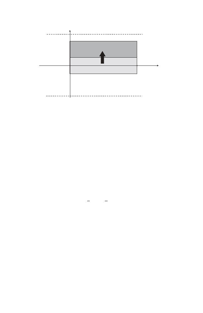
94
5 The minimal action and Hofer’s geometry
y
x
x
+1
max
x
max
1
-1
1/4
-1/4
3/4
Fig. 5.3. The map ϕ
1
K
shifts the lower rectangle onto the upper one
We will construct a Hamiltonian K
∈ H
0
such that
osc(H + H
◦ ϕ
1
K
)
≤ 1 − max V
in the following way. Lift everything to the universal cover
R×[−1, 1] of B
∗
T
1
.
Fix some point x
max
where the potential V attains its maximum. Suppose that
the outer separatrices, where H =
−1/2+max V , lie in the region {|y| ≤ 1/4}.
Neglecting small pertubations near
{x = x
max
} and {x = x
max
+ 1
}, we can
pick a K
∈ H
0
such that K(x, y) = x/2 for (x, y)
∈ [x
max
, x
max
+ 1]
×
[
−3/4, 3/4]. Then ϕ
1
K
shifts the rectangle [x
max
, x
max
+ 1]
× [−1/4, 1/4] onto
[x
max
, x
max
+ 1]
× [1/4, 3/4], so the set {−1/2 ≤ H ≤ −1/2 + max V } will be
mapped into the region where H
≥ −1/2 + max V ; see Fig. 5.3. Hence at each
point we have
0
≥ H + H ◦ ϕ
1
K
≥ −
1
2
+
−
1
2
+ max V
=
−1 + max V,
and our claim is proven.
This example prompts the following question.
Open problem. Suppose φ
∈ Ham(B
∗
T
n
) is generated by a convex Hamil-
tonian. Is it true that
d
∞
(id, φ) = osc α
∗
= α(0)?
If the answer were yes, this would mean that α
∗
, seen as a non–smooth
Hamiltonian, generated an asymptotically shortest connection. Thus, one
would be lead to the investigation of non–smooth Hamiltonians and sym-
plectic homeomorphisms in the context of Hofer geometry.

5.2 Estimates via the minimal action
95
Finally, Thm. 5.2.5 can be applied to obtain converse KAM–results, in
the sense that the location of invariant KAM–tori can be restricted to certain
domains in phase space. See [59, 58] for classical estimates involving minimal
orbits, and [12, 13] for results using Hofer’s metric d in the autonomous case.
For instance, Thm. 5.2.5 and Cor. 2.1.25 immediately imply the following
result.
Corollary 5.2.10. Suppose φ
∈ Ham(B
∗
T
n
) is generated by a convex Hamil-
tonian H
∈ H
0
whose flow possesses an invariant KAM–torus Λ. Then
S
1
H
t
|
Λ
dt
≥ −d
∞
(id, φ).

6
The minimal action and symplectic geometry
A hypersurface in a cotangent bundle is called convex if it bounds a fiberwise
strictly convex domain. In this chapter, we will deal with Lagrangian sub-
manifolds that lie in a convex hypersurface. A particularly important class of
examples is given by invariant tori in classical mechanics where the hyper-
surface is the level set of a convex Hamiltonian H. However, we will consider
this situation from the symplectic point of view, which is different from the
dynamical one. For instance, the property of being a Lagrangian section is
not a symplectic property.
In the first section, we establish a boundary rigidity phenomenon which,
roughly speaking, can be formulated as follows. Certain Lagrangian subman-
ifolds Λ in a convex hypersurface Σ cannot be mapped by a Hamiltonian
diffeomorphism into the domain bounded by Σ. In fact, under certain as-
sumptions on the dynamics on Λ, it is not possible to move Λ at all, so Λ is
indeed “boundary rigid”.
Furthermore, even when boundary rigidity fails, we often find another
phenomenon called non–removable intersection. In this case, the Lagrangian
submanifold Λ can partly be moved into the domain Σ but certain pieces of
Λ stay put. At this point the link between symplectic geometry and Mather–
Ma˜
n´
e theory appears. Namely, if Σ is the Ma˜
n´
e critical level set of H, these
“non–removable intersections” always contain the Aubry set of Σ.
Finally, we discuss Lagrangian submanifolds lying in the open domain U
bounded by a convex hypersurface. This leads to the notion of the shape
of U , a symplectic invariant that describes all Liouville classes that can be
represented by Lagrangian submanifolds in U . We will see that each class in
the shape of a convex domain can actually be represented by a Lagrangian
section. This allows us to give symplectic descriptions of, firstly, the stable
norm in Riemannian geometry and, secondly, the convex conjugate of Mather’s
minimal action.
This chapter is based on joint work with Gabriel P. Paternain and Leonid
Polterovich [81].
K.F. Siburg: LNM 1844, pp. 97–119, 2004.
c
Springer-Verlag Berlin Heidelberg 2004

98
6 The minimal action and symplectic geometry
6.1 Boundary rigidity in convex hypersurfaces
Let us recall some notation from Sect. 2.1.2. We denote by θ : T
∗
X
→ X
the cotangent bundle of a closed manifold X. It comes equipped with the
canonical symplectic form ω = dλ where λ is the Liouville form. We write
O
for the zero section, and denote by
L the class of all Lagrangian submanifolds
of T
∗
X which are Lagrangian isotopic to
O. The Liouville class of Λ ∈ L is
the class a
Λ
∈ H
1
(X,
R) defined as the preimage of [λ
Λ
] under the canonical
isomorphism H
1
(X,
R) → H
1
(Λ,
R); see Def. 2.1.23.
Definition 6.1.1. A Lagrangian submanifold Λ
∈ L is exact if a
Λ
= 0. The
class of all exact Lagrangian submanifolds in
L is denoted by L
0
.
Finally, we define what we mean by a convex hypersurface in a cotangent
bundle. Convexity will be a fundamental concept in this chapter. We refer to
[81] for more general results concerning the non–convex case.
Definition 6.1.2. A smooth, closed, fiberwise strictly convex hypersurface
Σ
⊂ T
∗
X is called a convex hypersurface.
Fiberwise strict convexity means that Σ intersects each fiber T
∗
x
X along a
hypersurface whose second fundamental form is positive definite.
In this section, we will establish a phenomenon called boundary rigidity
which, roughly speaking, can be formulated as follows. Certain Lagrangian
submanifolds lying in a convex hypersurface cannot be deformed into the
domain bounded by that hypersurface. Boundary rigidity may seem unrelated
to Mather–Ma˜
n´
e theory. However, as Thm. 6.2.11 will show, boundary rigidity
can be seen as a particular case of non–removable intersection, to be discussed
in Sect. 6.2. Moreover, the latter does have relations to Mather–Ma˜
n´
e theory,
as we will see in Sect. 6.2.2. Thus, there is indeed some indirect connection to
minimal action here.
6.1.1 Graph selectors for Lagrangian submanifolds
A particular example of an exact Lagrangian submanifold in T
∗
X is given by
the graph of the differential of a smooth function f : X
→ R. A general exact
Lagrangian submanifold Λ, of course, need not be a graph. However, we will
see that, even in this case, it is possible to extract a “graph part” inside Λ.
The following theorem was outlined by Sikorav (in a talk held at Chap-
eron’s seminar) and proven by Chaperon (in the framework of generating
functions) and Oh (via Floer homology).
Theorem 6.1.3 (Sikorav, Chaperon [17], Oh [80]). Let Λ
⊂ T
∗
X be an
exact Lagrangian submanifold in
L
0
. Then there exists a Lipschitz continuous
function Φ : X
→ R, which is smooth on an open set X
0
⊂ X of full measure,
such that
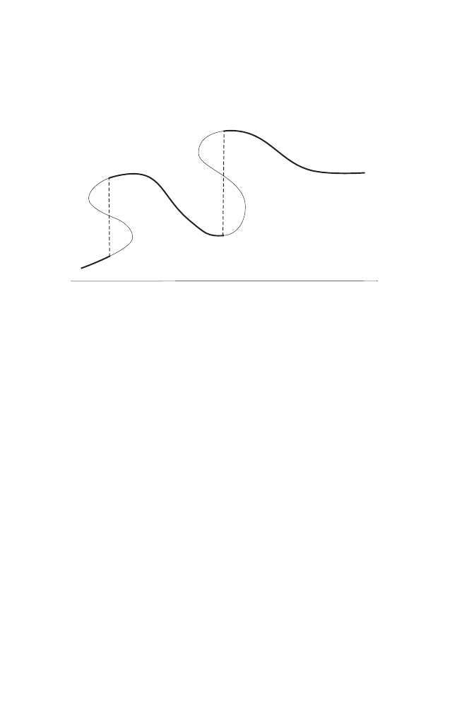
6.1 Boundary rigidity in convex hypersurfaces
99
(x, dΦ(x))
∈ Λ
(6.1)
for every x
∈ X
0
. Moreover, if dΦ(x) = 0 for all x
∈ X
0
then Λ coincides
with the zero section
O.
gr d
F
X
L
Fig. 6.1. A graph selector of an exact Lagrangian submanifold Λ
Definition 6.1.4. Let Λ
⊂ T
∗
X be an exact Lagrangian submanifold in
L
0
.
Any function Φ : X
→ R satisfying (6.1) is called a graph selector of Λ;
compare Fig. 6.1.
We will prove Thm. 6.1.3 by using generating functions quadratic at in-
finity, a powerful tool of symplectic topology in cotangent bundles. Although
this proof of Thm 6.1.3 is well known to experts, it was probably published
in [81]; we repeat it here for the convenience of the reader.
Let X be a closed manifold, and E a finite–dimensional real vector space.
Denote by
O
E
the zero section of T
∗
E and set
V := T
∗
X
× O
E
⊂ T
∗
X
× T
∗
E = T
∗
(X
× E).
Definition 6.1.5. A smooth function S : X
× E → R is called a generating
function quadratic at infinity if
S(x, ξ) = Q
x
(ξ)
outside a compact subset of X
× E, where Q
x
is a smooth family of nonde-
generate quadratic forms on E, and gr dS is transversal to V in T
∗
(X
× E).
In particular, W := gr dS
∩ V is a smooth closed submanifold of V of
the same dimension as X. Let χ : V
→ T
∗
X be the natural projection. One

100
6 The minimal action and symplectic geometry
can show that the restriction of χ to W is a Lagrangian immersion; see [4,
Sect. 19]. If χ
|
W
is an embedding then
Λ := χ(W )
is a Lagrangian submanifold of T
∗
X. In this case we say that Λ possesses a
generating function S quadratic at infinity, which means that
Λ =
{(x, d
x
S(x, ξ))
| x ∈ X, ξ ∈ E, d
ξ
S(x, ξ) = 0
}.
(6.2)
Proof (Thm. 6.1.3). Let Λ
∈ L
0
be given. Then Λ possesses a generating
function S : X
× E → R quadratic at infinity [99]. The graph selector Φ :
X
→ R will be defined by the following minimax procedure.
Fix a scalar product on E. Let B
x
: E
→ E be a self–adjoint operator
so that Q
x
(ξ) = (B
x
ξ, ξ). Denote by E
−
x
the subspace of E generated by all
eigenvectors of B
x
with negative eigenvalues. Set
E
a
x
:=
{ξ ∈ E | S
x
(ξ)
≤ a}
where a
∈ R and S
x
(
·) := S(x, ·). Pick an N > 0 such that S(x, ξ) = Q
x
(ξ)
whenever
|Q
x
(ξ)
| ≥ N. All quadratic forms Q
x
have the same index which
we denote by m. The homology group H
m
(E
N
x
, E
−N
x
;
Z
2
) is isomorphic to
Z
2
, and its generator A
x
is represented by the m-dimensional disc in E
−
x
whose boundary lies in
{Q
x
(ξ) =
−N}. For a ∈ [−N, N], consider the natural
morphism
I
a,x
: H
m
(E
a
x
, E
−N
x
;
Z
2
)
→ H
m
(E
N
x
, E
−N
x
;
Z
2
).
Now define the function Φ : X
→ R by
Φ(x) := inf
{a | A
x
∈ Image(I
a,x
)
}.
We claim that Φ has all the properties stated in Thm. 6.1.3.
It follows from the definition that each value Φ(x) is a critical value of S
x
.
Consider the subset X
0
⊂ X consisting of all those x for which S
x
is a Morse
function whose critical points have pairwise distinct critical values. In any
neighbourhood U of a point in X
0
there exists a smooth function ϕ : U
→ E
such that ϕ(x) is a critical point of S
x
and Φ(x) = S(x, ϕ(x)). Differentiating
with respect to x and taking into account that d
ξ
S(x, ϕ(x)) = 0 we get that
dΦ(x) = d
x
S(x, ϕ(x)). Thus, in view of (6.2), we have
(x, dΦ(x))
∈ Λ
for all x
∈ X
0
.
Claim. X
0
is an open subset of X of full measure.
Proof. Let θ : T
∗
X
→ X be the natural projection. Then S
x
is a Morse
function if, and only if, x is a regular value of θ
|
Λ
; see, e.g., [4, Sect. 21.2].

6.1 Boundary rigidity in convex hypersurfaces
101
Denote the set of these x
∈ X by X
1
. It is an open subset of X and, by Sard’s
Theorem, has full measure.
Let U
⊂ X
1
be a sufficiently small open subset. The critical points of S
x
depend smoothly on x
∈ U. Denote them by ϕ
1
(x), . . . , ϕ
d
(x), and put
a
ij
(x) := S(x, ϕ
i
(x))
− S(x, ϕ
j
(x))
for i
= j. Note that
da
ij
(x) = d
x
S(x, ϕ
i
(x))
− d
x
S(x, ϕ
j
(x))
= 0
since the map (x, ξ)
→ (x, d
x
S(x, ξ)) is an embedding of W = gr dS
∩ V into
T
∗
X. Therefore the sets
{x ∈ U | a
ij
(x) = 0
} are smooth hypersurfaces. It
follows from the definition of X
0
that
X
0
∩ U = U \ ∪
i
=j
{x ∈ U | a
ij
(x) = 0
},
so X
0
∩ U is indeed an open subset of full measure in X ∩ U.
Claim. If dΦ(x) = 0 for all x
∈ X
0
then Λ coincides with the zero section of
T
∗
X.
Proof. Identify X with the zero section of T
∗
X. Since X
0
has full measure,
its closure equals X. Hence Λ contains X since dΦ(x) = 0 for x
∈ X
0
, and
thus Λ = X.
Claim. Φ is a Lipschitz function on X.
Proof. Since X is compact it suffices to prove this locally. Let U
⊂ X be a
sufficiently small open subset. There exists a smooth family of linear au-
tomorphisms F
x
: E
→ E with x ∈ U, and a quadratic form Q on E,
such that Q
x
◦ F
x
= Q for all x
∈ U. It is easy to see that the function
S
(x, ξ) := S(x, F
x
ξ) is again a generating function of Λ over U quadratic a
infinity, and the functions Φ
and Φ coincide on U . Let us now work with S
instead of S, because the functions S
x
with x
∈ U equal the same quadratic
form Q outside a compact subset of E.
There exists a positive constant C such that for all x, y
∈ U and ξ ∈ E we
have
|S
(x, ξ)
− S
(y, ξ)
| ≤ C|x − y|.
(6.3)
Fix any > 0 and x
∈ U, and set
a(y) := Φ(x) + + C
|x − y|
where y
∈ U. It follows from inequality (6.3) that E
a(x)
x
⊂ E
a(y)
y
for all y
∈ U.
By definition, the pair (E
a(x)
x
, E
−N
) contains a relative cycle representing the
class A
x
. Therefore, the same holds for the pair (E
a(y)
y
, E
−N
). This implies
that Φ(y)
≤ a(y), so that

102
6 The minimal action and symplectic geometry
Φ(y)
− Φ(x) ≤ C|x − y| + .
Since > 0 was arbitrary we have
Φ(y)
− Φ(x) ≤ C|x − y|.
Interchanging x and y shows that Φ is Lipschitz continuous, as we wanted to
prove.
Summarizing, the function Φ satisfies all requirements and is indeed a
graph selector of Λ. This finishes the proof of Thm. 6.1.3.
6.1.2 Boundary rigidity
Let Σ be a hypersurface in a cotangent bundle T
∗
X. Denote by σ the charac-
teristic foliation of Σ, i.e., the 1–dimensional foliation tangent to the kernel of
ω
|
T Σ
. Note that σ is orientable and tangent to each Lagrangian submanifold
contained in Σ.
Given a convex hypersurface Σ, we denote by U
Σ
the closed(!) domain in
T
∗
X bounded by Σ.
Definition 6.1.6. An orientable 1–dimensional foliation on a closed manifold
is called conservative if it admits a non–vanishing tangent vector field whose
flow preserves a measure which is absolutely continuous with respect to some
(and hence any) Riemannian measure on that manifold.
Recall that a
Λ
∈ H
1
(X,
R) is the Liouville class of Λ ∈ L.
Theorem 6.1.7. Let Λ
∈ L be a Lagrangian submanifold that is contained in
some convex hypersurface Σ such that the restriction σ
|
Λ
of the characteristic
foliation is conservative. Let K
∈ L be
1
any Lagrangian submanifold lying
inside U
Σ
. Then
a
K
= a
Λ
⇐⇒ K = Λ.
In particular, Λ cannot be deformed inside U
Σ
by an exact Lagrangian
isotopy, i.e., by a Lagrangian isotopy that preserves the Liouville class. This
is the reason for the name “boundary rigidity”.
Proof. First of all, by the multi–dimensional Birkhoff theorem [11], Λ is a
Lagrangian section, i.e., Λ = gr ν for some closed 1–form ν. By applying the
symplectic shift (x, p)
→ (x, p − ν
x
) we may assume that Λ =
O is the zero
section. Note that the transformed hypersurface, again denoted by Σ, remains
convex.
Suppose now there is another Lagrangian submanifold K
⊂ U
Σ
, obtained
from Λ by an exact Lagrangian deformation. Thm. 6.1.3 implies that K admits
1
We denote Lagrangian submanifolds by Greek letters, so this is a capital
κ and
not a capital
k. . .
6.1 Boundary rigidity in convex hypersurfaces
103
a graph selector Φ : X
→ R, i.e., a function such that (x, dΦ(x)) ∈ K for all
x
∈ X
0
where X
0
⊂ X is a set of full measure.
Pick a convex Hamiltonian function H : T
∗
X
→ R such that Σ is a regular
level set of H. Since Λ is the zero section, the vector ∂
p
H(x, 0) gives the outer
normal direction to the hypersurface Σ
∩ T
∗
x
X
⊂ T
∗
x
X. Because Σ is convex
and K is contained in U
Σ
we have
dΦ(x)
· ∂
p
H(x, 0) < 0
(6.4)
for all x
∈ X
0
with dΦ(x)
= 0; see Fig 6.2.
S
S
U
H
p
K
Fig. 6.2. An illustration for the inequality (6.4)
Let V be a non–singular vector field on Λ, tangent to the characteristic
foliation, whose flow ϕ
t
preserves a measure µ which is absolutely continuous
with respect to some Riemannian measure. Then the Hamiltonian differential
equations for H show that V is collinear to the vector field ∂
p
H(x, 0) on Λ.
In view of (6.4), we may assume that
dΦ(x)
· V (x) < 0
(6.5)
for all x
∈ X
0
with dΦ(x)
= 0. On the other hand, we claim that
X
0
dΦ(x)
· V (x)dµ(x) = 0.
(6.6)
Then the theorem is an immediate consequence of (6.6). Indeed, combining
(6.6) and (6.5) we see that dΦ must vanish on X
0
, and hence
K =
O = Λ
in view of Thm. 6.1.3.

104
6 The minimal action and symplectic geometry
It remains to prove (6.6). Since the function Φ is Lipschitz continuous, the
function t
→ Φ(ϕ
t
(x))
− Φ(x) is also Lipschitz continuous on [0, 1] for every
x
∈ X. By Rademacher’s theorem, it is differentiable almost everywhere with
Φ(ϕ
1
(x))
− Φ(x) =
1
0
d
dt
Φ(ϕ
t
(x))dt.
Since the flow ϕ
t
preserves the measure µ we have
0 =
X
[Φ(ϕ
1
(x))
− Φ(x)] dµ(x) =
X
1
0
d
dt
Φ(ϕ
t
(x))dt dµ(x).
Since X
0
has full measure with respect to µ and since ϕ
t
preserves µ, we have
0 =
1
0
X
d
dt
Φ(ϕ
t
(x))dµ(x) dt
=
1
0
ϕ
−t
(X
0
)
dΦ(ϕ
t
(x))
· V (ϕ
t
(x))dµ(x) dt
=
1
0
X
0
dΦ(x)
· V (x)dµ(x) dt
=
X
0
dΦ(x)
· V (x)dµ(x).
This proves (6.6) and finishes the proof of the theorem.
As the following example shows, the assumption about the dynamics of
the characteristic foliation cannot be omitted.
Example 6.1.8. Consider Σ =
{H = 1} ⊂ T
∗
T
2
where
H(x
1
, x
2
, y
1
, y
2
) := (y
1
− sin x
1
)
2
+ (y
2
− cos x
1
)
2
.
(6.7)
Then Σ contains the zero section Λ =
O. However, the restriction σ|
O
of the
characteristic foliation is a Reeb foliation with exactly two limit cycles and,
therefore, not conservative. We claim that
O is not boundary rigid either.
Indeed, the exact Lagrangian torus K = gr df with
f (x
1
, x
2
) :=
− cos x
1
does lie in U
Σ
.
It is worth mentioning that K intersects Σ precisely at the two limit
cycles of the characteristic foliation. As we will see in Section 6.2.2, this is no
coincidence.

6.2 Non–removable intersections
105
6.2 Non–removable intersections
6.2.1 Mather–Ma˜
n´
e theory for minimizing hypersurfaces
In this section, we will see that many of the concepts presented in Sect. 2.2
do not really depend on the Lagrangian (or the Hamiltonian), but can rather
be formulated in the more general framework of convex hypersurfaces. We
concentrate on the torus
T
n
here, but all results and proofs in this section
are, word by word, valid for general closed manifolds; see [81].
As usual, we let θ : T
∗
T
n
→ T
n
be the cotangent bundle of the torus
T
n
,
equipped with the canonical symplectic form ω = dλ, where λ is the Liou-
ville form. Let Σ
⊂ T
∗
T
n
be a convex hypersurface, and σ its characteristic
foliation. Recall that σ is orientable; we choose the orientation defined by the
Hamiltonian vector field of any convex Hamiltonian having Σ as a regular
level set. Denote by U
Σ
the closed domain in T
∗
T
n
bounded by Σ.
Definition 6.2.1. A convex hypersurface Σ is minimizing if the interior of
U
Σ
does not contain a Lagrangian submanifold from
L
0
, but any open neigh-
bourhood of U
Σ
does.
Remark 6.2.2. It will turn out that, in defining minimizing hypersurfaces, one
can restrict to Lagrangian sections, rather than Lagrangian submanifolds.
Indeed, Thm. 6.3.4 ensures that we obtain precisely the same concept.
Remark 6.2.3. Suppose Σ is a minimizing hypersurface, and H is a convex
Hamiltonian having Σ as a regular level set H
−1
(k). Then, in view of (2.9),
k = c(L) is the Ma˜
n´
e critical value of the Lagrangian L corresponding to H.
Proposition 6.2.4. If a convex hypersurface Σ contains a Lagrangian sub-
manifold Λ
∈ L
0
then Σ is minimizing.
Proof. Any open neighbourhood of U
Σ
contains the Lagrangian submanifold
Λ
∈ L
0
. On the other hand, any other Lagrangian submanifold K
∈ L
0
must intersect Λ by Gromov’s theorem [36], so it cannot lie completely in the
interior of U
Σ
.
In the following, we are going to replace the concept of minimizing measure
for a convex Lagrangian L by a notion that depends only on the foliation σ
of an energy surface, and not on the particular choice of L. The appropriate
notion is that of a foliation cycle, introduced by Sullivan [100]. We briefly
review these ideas.
Let M be a closed n–dimensional manifold and let Ω
p
be the real vector
space of smooth p–forms on M . This vector space has a natural topology
which makes it a locally convex linear space. A continuous linear functional
f : Ω
p
→ R is called a p–current. With a natural topology, the space Ω
∗
p
of
p–currents becomes a locally convex linear space. Given a p–current f , we

106
6 The minimal action and symplectic geometry
define its boundary ∂f as the (p
− 1)–current such that ∂f(ω) = f(dω) for all
ω
∈ Ω
p
−1
. Currents with zero boundary are called cycles.
Given a foliation of M , Sullivan considers a distinguished subset of Ω
∗
1
that he calls foliation currents. This subset is defined as follows. Let V be
a vector field tangent to the foliation. For each x
∈ M, let δ
x
: Ω
1
→ R be
the Dirac 1–current defined by δ
x
(ω) := ω
x
(V (x)). By definition, foliation
currents are the elements of the closed convex cone in Ω
∗
1
generated by all the
Dirac currents.
Definition 6.2.5. A foliation cycle is a foliation current f
∈ Ω
∗
1
whose
boundary ∂f is zero.
Suppose now that V is a non–vanishing vector field on M . Then V defines
a map µ
→ f
V,µ
from measures to 1–currents given by
f
V,µ
(ω) :=
M
ω(V ) dµ.
Sullivan [100, Prop. II.24] shows that this map yields continuous bijections
between the following objects:
1. nonnegative measures on M and foliation currents;
2. measures on M , invariant under the flow of V , and foliation cycles.
In our setting, the manifold M will be a minimizing hypersurface Σ
⊂
T
∗
T
n
. Pick a convex Hamiltonian H such that
Σ = H
−1
(k)
is a regular level set, and let L be the corresponding Lagrangian. In view of
Remark 6.2.3, we have
k = c := c(L).
The following simple observation allows us to translate the notion of globally
minimizing measure into the languange of foliation cycles of the characteristic
foliation. Namely, if (x, v) is a point in the critical energy level E
−1
(c)
⊂ T T
n
then
L(x, v) + c = λ(d(V (x, v)))
(6.8)
where V is the Euler–Lagrange vector field of L, and the Legendre transform.
By Prop. 2.2.4, an invariant measure µ is globally minimizing if
T
T
n
L +
c dµ = 0. We also know from [25] that globally minimizing measures have their
support contained in the energy level E
−1
(c). Hence, the correct translation
of the notion of globally minimizing measures into the language of foliation
cycles is the following.
Definition 6.2.6. Let Σ be a minimizing hypersurface in T
∗
T
n
, and σ its
characteristic foliation. A foliation cycle f of σ is called minimizing if, and
only if, f (λ) = 0.

6.2 Non–removable intersections
107
Minimizing foliation cycles are precisely those which can be represented by
measures
∗
µ on T
∗
T
n
, where µ is some minimizing measure for some Hamil-
tonian H with Σ = H
−1
(k). Observe also that, if we have two Hamiltonians
H
1
, H
2
with the same regular level set Σ, and two minimizing measures µ
1
, µ
2
of H
1
, H
2
representing the same foliation cycle f , then the supports µ
1
and
µ
2
will coincide. Hence it makes sense to talk about the support of a foliation
cycle f of σ.
Now, the Mather set of a minimizing hypersurface Σ is defined as the clo-
sure of the union of the supports of all minimizing foliation cycles. It coincides
with the Mather set ˜
M
∗
in T
∗
T
n
of any convex Hamiltonian H having Σ as
regular level set.
In order to go further and define the Aubry set of Σ, we first have to
explain what a weak KAM solution should be in our setting. Given a point
(x, p)
∈ Σ, let Γ
±
(x, p) be the oriented positive (respectively, negative) half
of the leaf Γ
(x,p)
of σ through (x, p).
Definition 6.2.7. Let Σ be a minimizing hypersurface in T
∗
T
n
. A function
u
+
:
T
n
→ R is called a positive weak KAM solution of Σ if the following
two conditions hold:
1. u
+
is Lipschitz, and (x, du
+
(x))
∈ U
Σ
for almost every x
∈ T
n
;
2. for every x
∈ T
n
, there exists (x, p)
∈ Σ such that, if (y, p
) is a point in
Γ
+
(x,p)
, then
u
+
(y)
− u
+
(x) =
Γ
+
(x,p)
(y,p
)
λ
where Γ
+
(x,p)
(y, p
) is the oriented part of the leaf between (x, p) and (y, p
).
Similarly, a function u
−
:
T
n
→ R is called a negative weak KAM solution
of Σ if the following two conditions hold:
1. u
−
is Lipschitz, and (x, du
−
(x))
∈ U
Σ
for almost every x
∈ T
n
;
2. for every x
∈ T
n
, there exists (x, p)
∈ Σ such that, if (y, p
) is a point in
Γ
−
(x,p)
, then
u
−
(x)
− u
−
(y) =
Γ
−
(x,p)
(y,p
)
λ
where Γ
−
(x,p)
(y, p
) is the oriented part of the leaf between (y, p
) and (x, p).
Again, (6.8) shows that the sets
S
±
=
S
±
(Σ)
of positive (respectively, negative) weak KAM solutions depend only on Σ
and not on the particular choice of H. A pair of functions (u
−
, u
+
) is called
conjugate if u
±
∈ S
±
and u
−
= u
+
on the projected Mather set. Setting
I
(u
−
,u
+
)
:=
{x ∈ T
n
| u
−
(x) = u
+
(x)
}

108
6 The minimal action and symplectic geometry
for a pair of conjugate functions, we see as before that the functions u
±
are differentiable on
I
(u
−
,u
+
)
with the same derivative. Therefore, the map
x
→ du
−
(x) = du
+
(x) defines a set ˜
I
(u
−
,u
+
)
in T
∗
T
n
that contains the
Mather set of Σ. The Aubry set of Σ in T
∗
T
n
is then given by
˜
A
∗
= ˜
A
∗
(Σ) :=
∩
(u
−
,u
+
)
˜
I
(u
−
,u
+
)
where the intersection is taken over all pairs (u
−
, u
+
) of conjugate functions.
Having defined the Aubry set, one would now like to study the dynamics
on it and single out a certain dynamically relevant set inside the Aubry set.
For this, we need the following general definition.
Definition 6.2.8. Let ϕ
t
be a continuous flow on a compact metric space
(X, d). Given > 0 and T > 0, a strong (, T )–chain from x to y in X is a
finite sequence (x
i
, t
i
)
1≤i≤n
in X
× R such that x
1
= x, x
n
= y, and t
i
> T
for all i, as well as
n
−1
i=1
d(ϕ
t
i
(x
i
), x
i+1
) < .
A point x
∈ X is said to be strongly chain recurrent if for all > 0 and
T > 0, there exists a strong (, T )–chain that begins and ends in x. The set of
strongly chain recurrent points in X is denoted by
R.
The set
R contains the nonwandering set
2
, but it is easy to give examples
showing that it could be strictly larger. The notion of strong chain recur-
rence strengthens the usual notion of chain recurrence where one requires
only d(ϕ
t
i
(x
i
), x
i+1
) < for every single i.
Given a smooth orientable 1–dimensional foliation σ on a closed manifold,
the strong chain recurrent set of σ is the strong chain recurrent set of the flow
of any non–vanishing vector field V tangent to σ. In the case where σ is the
characteristic foliation of a hypersurface Σ
⊂ T
∗
T
n
, we denote by
R
∗
(σ)
⊂ Σ
the strong chain recurrent set in T
∗
T
n
, and by
R(σ) ⊂ T T
n
its preimage
under the Legendre transform.
Theorem 6.2.9. Let Σ be a minimizing hypersurface in T
∗
T
n
, and Λ
⊂ Σ
be an exact Lagrangian submanifold (not necessarily in
L). Then
R
∗
(σ
|
Λ
)
⊂ ˜
A
∗
(Σ).
In particular,
R
∗
(σ
|
Λ
) is a Lipschitz graph over
T
n
.
2
A point
x ∈ X is nonwandering if, and only if, for every neighbourhood U of x
there exists a
T > 1 such that φ
T
(
U) ∩ U = ∅; this implies that there are also
arbitrarily large
T with that property.

6.2 Non–removable intersections
109
Proof. Choose a convex Hamiltonian H having Σ as a regular level set, and
let L be the corresponding Lagrangian. For the proof, we will work in the
tangent bundle T
T
n
.
Endow T
T
n
and
T
n
with auxiliar Riemannian distances d
T
T
n
and d
T
n
in
such a way that the natural projection τ : T
T
n
→ T
n
does not increase the
distances. Consider (x, v)
∈ R and consider the curve γ with
γ(t) := τ (ϕ
t
L
(x, v)).
In view of Prop. 2.2.16, it suffices to show that γ is static. This will imply
that
R ⊂ ˜
A.
Take s
≤ t and set
ξ := ϕ
s
L
(x, v)
,
η := ϕ
t
L
(x, v).
We claim that, for any given > 0, there exists a strong (, 1)–chain from
η to ξ. To see this, let us start with a strong (δ, T )–chain from x
1
:= η to
x
n+1
:= η where T > 1 is large compared to t
− s, and replace x
n+1
by
ϕ
t
n
−(t−s)
L
(x
n
). If δ > 0 is chosen sufficiently small, the point ϕ
t
n
−(t−s)
L
(x
n
)
lies in an –neighbourhood of ξ, and we obtain a strong (, 1)–chain from η to
ξ. Let us call this chain (η
i
, t
i
)
1≤i≤n+1
with η
1
= η, η
n+1
= ξ, t
i
> 1, and
n
i=1
d
T
T
n
(ϕ
t
i
L
(η
i
), η
i+1
) < .
Set p
i
:= τ (η
i
) and q
i
:= τ (ϕ
t
i
L
(η
i
)). Using (6.8) and the fact that Λ is exact,
we have
Φ
c
(p
i
, q
i
)
≤ A
L+c
(τ
◦ ϕ
t
L
(η
i
)
|
[0,t
i
]
) = g(φ
t
i
(η
i
))
− g(η
i
),
(6.9)
where g :
−1
(Λ)
→ R is a smooth function such that d(g ◦
−1
|
Λ
) = λ
|
Λ
.
Recall that the action potential Φ
c
satisfies the triangle inequality
Φ
c
(x, y)
≤ Φ
c
(x, z) + Φ
c
(z, y)
and Φ
c
(x, x) = 0. Hence we can estimate
Φ
c
(p
1
, p
n+1
)
≤ Φ
c
(p
1
, q
1
) + Φ
c
(q
1
, p
2
) + . . . + Φ
c
(p
n
, q
n
) + Φ
c
(q
n
, p
n+1
).
Given p, q
∈ T
n
let γ : [0, d
T
n
(p, q)]
→ T
n
be a unit speed minimizing geodesic
from p to q. Then we have
Φ
c
(p, q)
≤
d
Tn
(p,q)
0
(L + c)(t, γ(t), ˙γ(t)) dt
≤ κ
1
d
T
n
(p, q)
where κ
1
:= max
{|(L + c)(x, v)| | (x, v) ∈ T T
n
and
|v| = 1}. Thus

110
6 The minimal action and symplectic geometry
i
Φ
c
(q
i
, p
i+1
)
≤ κ
1
i
d
T
n
(q
i
, p
i+1
)
≤ κ
1
.
(6.10)
Combining (6.10) and(6.9), we obtain
Φ
c
(p
1
, p
n+1
)
≤
i
Φ
c
(p
i
, q
i
) + Φ
c
(q
i
, p
i+1
)
≤ κ
1
+ κ
2
+ g(ξ)
− g(η),
where κ
2
is a Lipschitz constant for g. On the other hand,
Φ
c
(p
n+1
, p
1
)
≤ A
L+c
(γ
|
[s,t]
) = g(η)
− g(ξ).
Therefore, we obtain
0 = Φ
c
(p
1
, p
1
)
≤ Φ
c
(p
1
, p
n+1
) + Φ
c
(p
n+1
, p
1
)
≤ (κ
1
+ κ
2
).
Since > 0 was arbitrary, we conclude that
Φ
c
(p
1
, p
n+1
) + Φ
c
(p
n+1
, p
1
) = 0.
Using the triangle inequality for Φ
c
as in the proof of Prop. 2.2.16, we finally
see that γ is a static curve.
6.2.2 The Aubry set and non–removable intersections
Let Σ
⊂ T
∗
T
n
be a convex hypersurface bounding the closed domain U
Σ
.
We want to study the following question. Suppose Σ contains a Lagrangian
submanifold Λ
∈ L. Is it possible to deform Λ into the interior of U
Σ
? In
other words, if you think of Σ being an energy surface H
−1
(k) of a convex
Hamiltonian, can one push Λ into the region where H < k? Compare Fig. 6.3
for an illustration.
Of course, there is no problem in deforming Λ into the interior of U
Σ
by
a Lagrangian isotopy: just apply symplectic shifts (x, y)
→ (x, y − ν
x
) with
some closed 1–form ν. So the whole point is to ask for exact Lagrangian
isotopies which preserve the Liouville class. In fact, one can forgo the isotopy
and ask whether there exists another Lagrangian K in the interior of U
Σ
with
a
K
= a
Λ
.
It turns out that there are situations where any such Lagrangian K cannot
lie completely in the interior of U
Σ
. In fact, we will see that it cannot even be
disjoint from Λ. In this case we say that a non–removable intersection phe-
nomenon occurs for Λ. It is clear now that boundary rigidity from Sect. 6.1.2
can be seen as a particular case of non–removable interesctions.
The following theorem establishes a non–removable intersection phe-
nomenon in the context of Mather–Ma˜
n´
e theory.
Theorem 6.2.10. Let Σ be a minimizing hypersurface such that U
Σ
contains
a Lagrangian submanifold Λ
∈ L
0
. Then
˜
A
∗
⊂ Λ ∩ Σ.
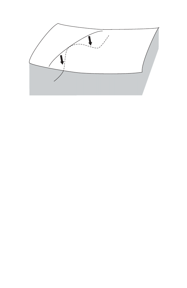
6.2 Non–removable intersections
111
L
K
S
S
U
Fig. 6.3. A deformation of Λ into the domain U
Σ
Proof. Let u :
T
n
→ R be a graph selector of Λ, whose existence is guaranteed
by Thm. 6.1.3. The function u is Lipschitz continuous and satisfies
(x, du(x))
∈ Λ
(6.11)
for every point x
∈ T
n
where U is differentiable; these points form a set of
full measure. Choose a Hamiltonian H such that Σ is a regular level set of H.
Rem. 6.2.3 shows that
Σ = H
−1
(c)
where c = c(L) is the critical value of the Lagrangian L corresponding to H.
By Rem. 2.2.9 and Thm. 2.2.11, there exists a pair of conjugate functions
(u
−
, u
+
) with
u
+
≤ u ≤ u
−
.
At any point x
∈ I
(u
−
,u
+
)
, the three functions are differentiable with the same
derivative. Hence du(x) exists for each x
∈ I
(u
−
,u
+
)
and satisfies (x, du(x))
∈
Σ.
We claim that we have
(x, du(x))
∈ Λ
for every x
∈ I
(u
−
,u
+
)
. This is the main step of the proof since, a priori, we
only know that this is true for almost every x.
In order to prove our claim we let
C
x
(Λ) := conv(Λ
∩ T
∗
x
T
n
)
denote the convex hull of Λ
∩ T
∗
x
T
n
. The set Λ
∩ T
∗
x
T
n
is compact, so C
x
(Λ)
is compact, too, as well as

112
6 The minimal action and symplectic geometry
C(Λ) :=
∪
x
∈T
n
C
x
(Λ).
This implies that for any point x of differentiability of u we have
(x, du(x))
∈ C(Λ);
see [90]. But since Σ
∩T
∗
x
T
n
is strictly convex, and (6.11) holds with Λ
⊂ U
Σ
,
the point (x, du(x)) is an extreme point of C
x
(Λ). But any extreme point in
the convex hull conv(Λ
∩ T
∗
x
T
n
) belongs to Λ
∩ T
∗
x
T
n
itself, and therefore we
have (x, du(x))
∈ Λ. This proves our claim.
Now, by definition of the Aubry set, ˜
A is contained in ˜I
(u
−
,u
+
)
for any
pair of conjugate functions. This finishes the proof of the theorem.
As mentioned before, Thm. 6.2.10 can be applied in order to estab-
lish boundary rigidity results. The following theorem is a generalization of
Thm. 6.1.7, because the assumption on the dynamics on Σ are weaker. Note,
however, that the proof of Thm. 6.1.7 did not need Mather–Ma˜
n´
e theory.
Theorem 6.2.11. Let Λ
∈ L be a Lagrangian submanifold contained in some
convex hypersurface Σ such that the restriction σ
|
Λ
of the characteristic foli-
ation is strongly chain recurrent. Let K
∈ L be any Lagrangian submanifold
lying inside U
Σ
. Then
a
K
= a
Λ
⇐⇒ K = Λ.
Proof. Since the multi–dimensional Birkhoff theorem is valid if σ
|
Λ
is chain
recurrent [11, Prop. 1.2], we may, as in the proof of Thm. 6.1.7, apply a
symplectic shift and assume that Λ =
O ⊂ T
∗
T
n
. By Prop. 6.2.4 the shifted
hypersurface obtained from Σ is still minimizing since it contains
O. But then
Thm. 6.2.9 implies that
O ⊂ ˜
A
∗
. Since the natural projection θ
|
˜
A
∗
: ˜
A
∗
→ A
is a homeomorphism [29] we must have
˜
A
∗
=
O.
Thm. 6.1.3 states that K possesses a graph selector; choose one. As in the
proof of Thm. 6.2.10, it will be differentiable at every point in θ( ˜
A
∗
) =
T
n
with zero derivative. But this means that K coincides with the zero section,
and so
K =
O = Λ
as we wanted to prove.
Example 6.2.12 (cont.). Let us come back to Ex. 6.1.8. Recall that we consider
the zero section
O of T
∗
T
2
lying inside the convex hypersurface
Σ =
{(y
1
− sin x
1
)
2
+ (y
2
− cos x
1
)
2
= 1
}.
The restriction σ
|
O
of the characteristic foliation is a Reeb foliation; see
Fig. 6.4. Denote by Z the union of the two limit cycles. Note that Z is the
strong chain recurrent set of σ
|
O
, and so, by Thm. 6.2.9, we have
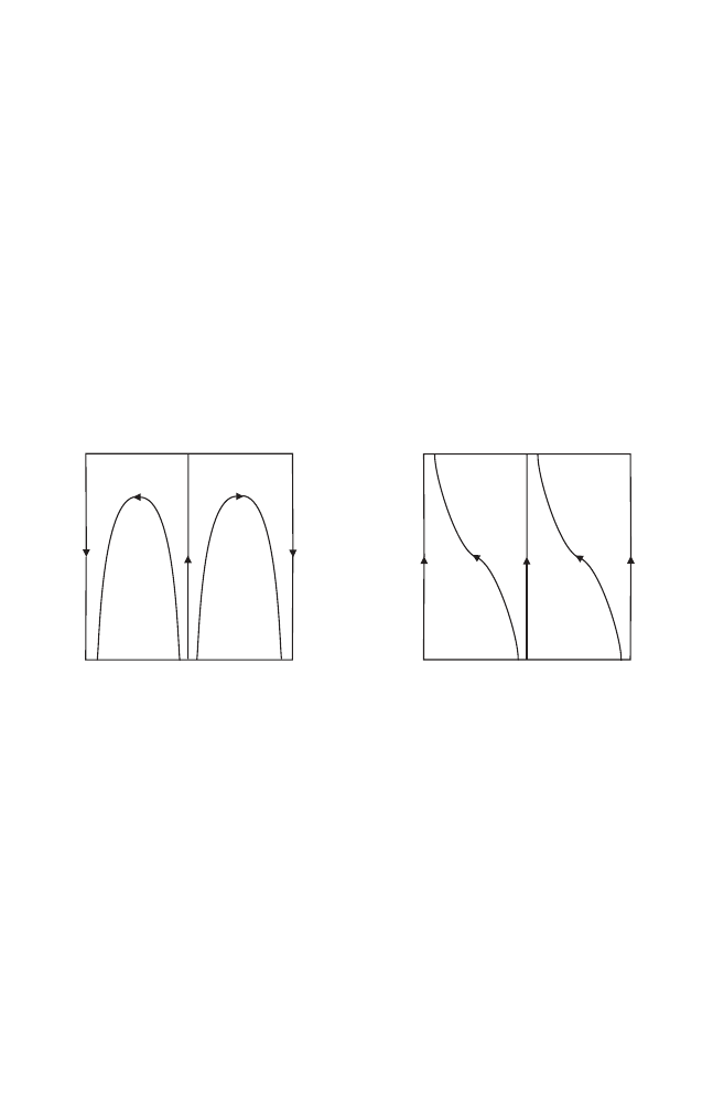
6.2 Non–removable intersections
113
Z
⊂ ˜
A
∗
.
(6.12)
Since Σ contains the zero section it is minimizing in view of Prop. 6.2.4.
Applying Thm. 6.2.10, we see that
Z
⊂ K ∩ Σ
for every Lagrangian submanifold K
∈ L
0
contained in U
Σ
. This explains the
remark at the end of Ex. 6.1.8.
In fact, we can show that the Aubry and Mather sets of Σ coincide with
Z:
˜
M
∗
= Z = ˜
A
∗
.
Indeed, we noticed in Ex. 6.1.8 that the graph of df with f (x
1
, x
2
) =
− cos x
1
intersects Σ precisely along Z. Hence, by Thm. 6.2.10, we obtain ˜
A
∗
⊂ Z.
Together with (6.12) this yields Z = ˜
A
∗
. Furthermore, each of the two limit
cycles in Z is a foliation cycle; it vanishes on the Liouville form since λ
|
O
= 0.
Hence we also see that ˜
M
∗
= Z.
Fig. 6.4. The dynamics on the zero section in Ex. 6.2.12 (left) and Ex. 6.2.13 (right)
Example 6.2.13. Let us investigate the zero setion in T
∗
T
2
with different dy-
namics. For this, we pick a diffeomorphism f : S
1
→ S
1
with exactly two fixed
points such that the fixed points are neither attractors nor repellors. Let V
be the unit norm vector field on
T
2
obtained by suspending f . Write
V (x
1
, x
2
) =: (a
1
(x
1
, x
2
), a
2
(x
1
, x
2
))
and let H be the convex Hamiltonian
H(x
1
, x
2
, y
1
, y
2
) := (y
1
− a
1
(x
1
, x
2
))
2
+ (y
2
− a
2
(x
1
, x
2
))
2
.
Consider the convex hypersurface Σ :=
{H = 1} ⊂ T
∗
T
2
. Since Σ contains
the zero section
O it is minimizing in view of Prop. 6.2.4. If we identify O

114
6 The minimal action and symplectic geometry
with
T
2
then V is tangent to the characteristic foliation σ
|
O
. Note that σ
|
O
is strongly chain recurrent, hence
O is boundary rigid by Thm. 6.2.11.
In this example, we will find that
˜
M
∗
= Z
= O = ˜
A
∗
.
Indeed, Theorems 6.2.9 and 6.2.10 yield ˜
A
∗
⊂ O and O ⊂ ˜
A
∗
, respectively, so
˜
A
∗
=
O. On the other hand, the same argument as in Ex. 6.2.12 shows that
˜
M
∗
= Z.
6.3 Symplectic shapes and the minimal action
This section deals with certain symplectic properties of domains in a cotangent
bundle (T
∗
X, ω = dλ) of some closed manifold X. Namely, given some domain
U
⊂ T
∗
X, we ask which cohomology classes in H
1
(X,
R) can be represented as
Liouville classes of Lagrangian submanifolds lying in U . We refer to Def. 2.1.23
for the definition of the Liouville class of a Lagrangian submanifold in
L .
Definition 6.3.1. The shape of a subset U
⊂ T
∗
X is defined as
sh(U ) :=
{a
Λ
∈ H
1
(X,
R) | Λ ∈ L with Λ ⊂ U}.
The notion of shape allows an elegant formulation of Gromov’s theorem
on Lagrangian intersections proven in [36]: shapes of disjoint subsets in T
∗
X
are disjoint. As a consequence, if Σ is a hypersurface in T
∗
X bounding the
domain U
Σ
, then every Lagrangian submanifold Λ
∈ L with a
Λ
∈ ∂sh(U
Σ
)
must intersect Σ.
The shape of U is an exact symplectic invariant of U ; in particular, it is
preserved by Hamiltonian diffeomorphisms of T
∗
X. From the dynamical point
of view, a very important class of Lagrangian submanifolds are Lagrangian
sections, i.e., graphs of closed 1–forms. This leads to the following definition.
Definition 6.3.2. The sectional shape of a subset U
⊂ T
∗
X is defined as
sh
0
(U ) :=
{a
Λ
∈ H
1
(X,
R) | Λ ∈ L is a section with Λ ⊂ U}.
It is clear that
sh
0
(U )
⊂ sh(U).
In contrast to the shape, however, the sectional shape is not preserved under
Hamiltonian diffeomorphisms and does, therefore, not belong to the realm of
symplectic geometry.
The question arises whether there are natural situations in which the sec-
tional shape and the shape coincide. We will see that this is the case for the
class of fiberwise convex domains. For simplicity, we call a subset U
⊂ T
∗
X
convex if it is fiberwise convex.

6.3 Symplectic shapes and the minimal action
115
6.3.1 Lagrangian sections in convex domains
Suppose U
⊂ T
∗
X be an open convex domain. We want to prove that every
class a
∈ sh(U) can be represented by a Lagrangian section of the cotangent
bundle. Indeed, this an immediate consequence of the following theorem
3
. Let
us denote the fiberwise convex hull of a set S
⊂ T
∗
X by conv(S).
Theorem 6.3.3. Given a Lagrangian submanifold Λ
∈ L, the fiberwise convex
hull conv(W ) of any neighbourhood W of Λ contains a Lagrangian section
Λ
0
∈ L with a
Λ
0
= a
Λ
.
Proof. We may assume that Λ is an exact Lagrangian submanifold, by apply-
ing the symplectic shift (x, y)
→ (x, y − ν
x
) where ν is the closed 1–form on
X representing the Liouville class a
Λ
.
Let Φ : X
→ R be a graph selector of Λ as described in Thm. 6.1.3; namely,
Φ is Lipschitz continuous, smooth on an open subset X
0
⊂ X of full measure,
and satisfies
gr dΦ
|
X
0
⊂ Λ.
(6.13)
The proof of Thm. 6.3.3 is divided into two steps.
Smoothing: We are going to regularize the Lipschitz continuous function Φ by
a convolution argument, similar to the proof of Prop. 7 in [22]. For this, we
embed X into some Euclidean space
R
N
. Denote by V
r
the r–neighbourhood
of X in
R
N
, where r > 0 is chosen small enough so that the orthogonal
projection
π : V
r
→ X
is well defined. We extend Φ : X
→ R to a function ¯
Φ : V
r
→ R by setting
¯
Φ := Φ
◦ π.
For each s
∈ (0, r/2) we pick a smooth cut–off function u : [0, ∞) → [0, ∞)
with support in [0, s] such that u is constant near 0 and satisfies
R
N
u(
|z|)dz = 1.
Define the function ¯
Ψ : V
s
→ R to be the convolution
¯
Ψ (z) := ( ¯
Φ
∗ u)(z) =
R
N
¯
Φ(y)u(
|z − y|)dy.
Since ¯
Φ is Lipschitz continuous, it is differentiable almost everywhere and
weakly differentiable. Therefore, ¯
Ψ is a smooth function on V
s
with
3
A slightly more general version of it was proven independently in [30, App.].

116
6 The minimal action and symplectic geometry
d ¯
Ψ (z) =
R
N
¯
Φ(y)d
z
u(
|z − y|)dy
=
−
R
N
¯
Φ(y)d
y
u(
|z − y|)dy
=
R
N
d ¯
Φ(y)u(
|z − y|)dy.
Denote by
Ψ := ¯
Ψ
|
X
the restriction of ¯
Ψ to X, and let B
s
(x)
⊂ V
s
⊂ R
N
be the open ball of radius
s centered at x
∈ X. Because X
0
has full measure in X, we conclude that
dΨ (x) =
π
−1
(X
0
)∩B
s
(x)
d ¯
Φ(y)
|
T
x
X
u(
|x − y|)dy.
(6.14)
Note that, for this formula to make sense, we identify each T
y
R
N
(where
y
∈ R
N
) with
R
N
, and each T
x
X (where x
∈ X) with a linear subspace of
R
N
.
Analising formula (6.14): For each x
∈ X, we write
P
x
: T
x
R
N
∼
=
R
N
→ T
x
X
for the orthogonal projection. Write
| · | for the Euclidean norm on R
N
and
| · |
∗
for the dual norm on (
R
N
)
∗
. Introduce a distance function on T
∗
X by
setting
dist((x, ξ), (y, η)) :=
|x − y| + |ξ ◦ P
x
− η ◦ P
y
|
∗
.
(6.15)
For x
∈ X, we define the set
G
s
(x) :=
{(x, d ¯
Φ(y)
|
T
x
X
))
| y ∈ π
−1
(X
0
)
∩ B
s
(x)
} ⊂ T
∗
X.
For a subset Z
⊂ T
∗
X, we denote by W
(Z) the –neighbourhood of Z with
respect to the distance defined in (6.15).
Claim. For every > 0 there is an s > 0 such that
G
s
(x)
⊂ W
/2
(gr dΦ
|
X
0
)
for each x
∈ X.
Proof. Pick any point
η
1
= (x, d ¯
Φ(y)
|
T
x
X
)
∈ G
s
(x)
with x
∈ X and y ∈ π
−1
(X
0
)
∩B
s
(x). We will show that the distance between
η
1
and
η
2
:= (π(y), dΦ(π(y)))
∈ gr dΦ|
X
0

6.3 Symplectic shapes and the minimal action
117
becomes as small as we wish, uniformly in x and y, when s
→ 0.
Indeed, denote by c > 0 the Lipschitz constant of Φ with respect to the
induced distance on X
⊂ R
N
. Let Q
y
be the differential of the projection π
at y, where we consider Q
y
as an endomorphism of
R
N
. Finally, write
· for
the operator norm on End(
R
N
). Now we can estimate
dist(η
1
, η
2
) =
|x − π(y)| + |d ¯
Φ(y)
|
T
x
X
◦ P
x
− dΦ(π(y)) ◦ P
π(y)
|
∗
=
|x − π(y)| + |dΦ(π(y)) ◦ Q
y
◦ P
x
− dΦ(π(y)) ◦ P
π(y)
|
∗
≤ |x − y| + |y − π(y)| + cQ
y
◦ P
x
− P
π(y)
.
Note that
|x − y| + |y − π(y)| ≤ 2s → 0 as s → 0. Therefore, it remains to
handle the term
Q
y
◦ P
x
− P
π(y)
. Using that P
x
= P
π(y)
= 1 we obtain
Q
y
◦ P
x
− P
π(y)
= Q
y
◦ P
x
− P
π(y)
◦ P
x
+ P
π(y)
◦ P
x
− P
π(y)
◦ P
π(y)
≤ Q
y
− P
π(y)
+ P
x
− P
π(y)
→ 0
as s
→ 0, and the convergence is uniform in x ∈ X and y ∈ B
s
(x).
This finishes the proof of our claim.
Now the proof of Thm. 6.3.3 follows immediately. Namely, given any > 0,
we choose s as given in our claim. Then (6.14) and (6.13) imply that
(x, dΨ (x))
∈ conv(W
/2
(
G
s
(x)))
⊂ conv(W
(gr dΦ
|
X
0
))
⊂ conv(W
(Λ))
for each x
∈ X. Therefore, the Lagrangian section Λ
0
:= gr dΨ satisfies
Λ
0
⊂ conv(W
(Λ)).
Since > 0 was arbitrary the proof of Thm. 6.3.3 is completed.
6.3.2 Symplectic descriptions of the stable norm and the minimal
action
In this final section, we focus on Lagrangian submanifolds contained in some
convex subset of a cotangent bundle. Recall Def. 6.3.1 and Def. 6.3.2 of the
shape and sectional shape of a subset U
⊂ T
∗
T
n
, respectively. We mentioned
the fact that the shape is preserved under Hamiltonian diffeomorphisms,
whereas the sectional shape is not.
The following theorem is the main result of this section. It states that for
open convex sets U
⊂ T
∗
T
n
both notions coincide.
Theorem 6.3.4. Let U
⊂ T
∗
T
n
be open and convex. Then every class a
∈
sh(U ) can be represented by a Lagrangian section of the cotangent bundle. In
other words,
sh
0
(U ) = sh(U ).

118
6 The minimal action and symplectic geometry
Proof. Let a
∈ sh(U) be represented by a Lagrangian Λ ∈ L contained in U.
Since U is open and convex, it contains the fiberwise convex hull conv(W ) of
some small neighbourhood W of Λ. Now, Thm. 6.3.3 guarantees that there is
a Lagrangian section Λ
0
⊂ W with a
Λ
0
= a
Λ
.
By taking convex combinations of Lagrangian sections, the following is a
direct consequence of Thm.6.3.4.
Corollary 6.3.5. The shape of an open convex subset of T
∗
T
n
is an open
convex subset of H
1
(
T
n
,
R).
Note that the shape of an open subset is always open; this follows imme-
diately from Weinstein’s Lagrangian neighbourhood theorem. Therefore, the
main statement here is about convexity.
Example 6.3.6. Take a Riemannian metric g on
T
n
and consider the corre-
sponding open unit co–ball bundle
B
∗
g
T
n
:=
{(x, p) ∈ T
∗
T
n
| |p|
g
< 1
}.
In geometric measure theory, one defines a particular norm on H
1
(
T
n
,
R),
called the stable norm. Let us illustrate the stable co–norm here, i.e., the corre-
sponding dual norm
· on H
1
(
T
n
,
R). If we write (h) for the minimal length
of a closed geodesic representing an integer homology class h
∈ H
1
(
T
n
,
Z) then
h := lim
N
→∞
(N h)
N
.
Let us denote by B
∗
st
T
n
⊂ H
1
(
T
n
,
R) the open unit ball of the stable norm.
Gromov proved [37] that
B
∗
st
T
n
= sh
0
(B
∗
g
T
n
).
In view of Thm. 6.3.4, we now have the following result.
Theorem 6.3.7. Let g be a Riemannian metric on
T
n
and B
∗
g
T
n
the corre-
sponding unit ball bundle. Then the unit ball of the stable norm coincides with
the shape of B
∗
g
T
n
:
B
∗
st
T
n
= sh(B
∗
g
T
n
).
Thus, for the Riemannian case, Theorem 6.3.4 leads to a geometric de-
scription of the symplectic shape of a Riemannian unit co–ball bundle and,
vice versa, to a symplectic characterization of the unit stable norm ball.
We come back to our favourite setting and consider a convex Lagrangian
L : T
T
n
→ R. Recall from Ch. 2 that, associated to L, there is the minimal
action α : H
1
(
T
n
,
R) → R and its convex conjugate α
∗
: H
1
(
T
n
,
R) → R. The
following result translates Mather’s variational construction of the minimal
action into the language of symplectic geometry.

6.3 Symplectic shapes and the minimal action
119
Theorem 6.3.8. Let L : T
T
n
→ R be a convex Lagrangian, and H : T
∗
T
n
→
R the corresponding convex Hamiltonian. Then the convex conjugate α
∗
:
H
1
(
T
n
,
R) → R of the minimal action of L can be written as
α
∗
(c) = inf
{k ∈ R | c ∈ sh({H < k})}.
Proof. Recall from (2.9) that the critical value c(L) of L allows the represen-
tation
c(L) = inf
u
max
x
H(x, du(x)).
It describes c(L) as the least value k such that the sublevel set
{H < k}
contains an exact Lagrangian section. Moreover, Cor. 2.2.6 showed that the
convex conjugate α
∗
: H
1
(
T
n
,
R) → R of the minimal action can be calculated
via the critical value as
α
∗
([ν]) = c(L
− ν).
Therefore, we have
α
∗
(c) = inf
{k ∈ R | c ∈ sh
0
(
{H < k})}.
Since H is convex, each sublevel set
{H < k} is a (fiberwise) convex subset
of T
∗
T
n
. Therefore, Thm. 6.3.4 implies that
sh
0
(
{H < k}) = sh({H < k}).
This finishes the proof of Thm. 6.3.8.

References
1. Amiran, E. (1988): Caustics and evolutes for convex planar domains. J. Diff.
Geom., 28, 345–357
2. Amiran, E. (1993): A dynamical approach to symplectic and spectral invariants
for billiards. Commun. Math. Phys., 154, 99–110
3. Anderson, K., Melrose, R. (1977): The propagation of singularities along gliding
rays. Invent. math., 41, 23–95
4. Arnold, V.I., Gusein–Zade, S.M., Varchenko, A.N. (1985): Singularities of dif-
ferentiable maps. Vol. I. The classification of critical points, caustics and wave
fronts. Birkh¨
auser
5. Aubry, S. (1983): The twist map, the extended Frenkel–Kontorova model and
the devil’s staircase. Physica, 7D, 240–258
6. Bangert, V. (1988): Mather sets for twist maps and geodesics on tori. In: Kirch-
graber, U., Walther, H.–O. (eds) Dynamics Reported 1. J. Wiley & Sons and
B.G. Teubner
7. Bangert, V. (1994): Geodesic rays, Busemann functions and monotone twist
maps. Calc. Var. Partial Differ. Equ., 2, 49–63
8. Bernard, P. (2003): The action spectrum near positive definite invariant tori.
Bull. Soc. math. France, 131, 603–616
9. Bialy, M. (1993): Convex billiards and a theorem by E. Hopf. Math. Z., 214,
147–154
10. Bialy, M., Polterovich, L. (1992): Hamiltonian systems, Lagrangian tori and
Birkhoff’s theorem. Math. Ann., 292, 619–627
11. Bialy, M., Polterovich, L. (1992): Hamiltonian diffeomorphisms and Lagrangian
distributions. Geom. Funct. Anal., 2, 173–210
12. Bialy, M., Polterovich, L. (1994): Geodesics of Hofer’s metric on the group of
Hamiltonian diffeomorphisms. Duke Math. J., 76, 273–292
13. Bialy, M., Polterovich, L. (1996): Invariant tori and symplectic topology. Amer.
Math. Soc. Transl., 171, 23–33
14. Billingsley, P. (1968): Convergence of probability measures. Wiley
15. Birkhoff, G.D. (1922): Surface transformations and their dynamical applica-
tions. Acta Math., 43, 1–119 [Reprinted in: Collected Mathematical Papers.
AMS 1950]
16. Birkhoff, G.D. (1932): Sur quelques courbes ferm´
ees remarquables. Bull. Soc.
Math. France, 60, 1–26 [Reprinted in: Collected Mathematical Papers. AMS
1950]
K.F. Siburg: LNM 1844, pp. 121–125, 2004.
c
Springer-Verlag Berlin Heidelberg 2004

122
References
17. Chaperon, M. (1991): Lois de conservation et g´
eom´
etrie symplectique. C. R.
Acad. Sci., 312, 345–348
18. Colin de Verdi`
ere, Y. (1973): Spectre du Laplacien et longueurs des g´
eod´
esiques
p´
eriodiques I. Comp. Math., 27, 83–106
19. Colin de Verdi`
ere, Y. (1984): Sur les longueurs des trajectoires p´
eriodiques d’un
billard. In: Dazord, Desolneux (eds) G´
eom´
etrie symplectique et de contact.
Sem. Sud–Rhod. G´
eom.
20. Contreras, G., Delgado, J., Iturriaga, R. (1997): Lagrangian flows: the dy-
namics of globally minimizing orbits II. Bol. Soc. Bras. Mat., Nova Ser., 28,
155–196
21. Contreras, G., Iturriaga, R. (1999): Global Minimizers of Autonomous La-
grangians. 22
o
Col´
oquio Brasiliero de Matem´
atica. IMPA
22. Contreras, G., Iturriaga, R., Paternain, G., Paternain, M. (1999): Lagrangian
graphs, minimizing measures and Ma˜
n´
e’s critical values. Geom. Funct. Anal.,
8, 788–809
23. Contreras, G., Iturriaga, R., Paternain, G., Paternain, M. (2000): The Palais–
Smale condition and Ma˜
n´
e’s critical value. Ann. Henri Poincar´
e, 1, 655–684
24. Cornfeld, I.P., Fomin, S.V., Sinai, Y.G. (1982): Ergodic Theory. Springer
25. Dias Carneiro, M.J. (1995): On minimizing measures of the action of au-
tonomous Lagrangians. Nonlinearity, 8, 1077–1085
26. Douady, R. (1988): Stabilit´
e ou instabilit´
e des points fixed elliptiques. Ann.
Sci. ´
Ec. Norm. Sup., 21, 1–46
27. Eliashberg, Y., Polterovich, L. (1993): Biinvariant metrics on the group of
Hamiltonian diffeomorphisms. Int. J. Math., 4, 727–738
28. Fathi, A. (1983): Appendix to Ch. I of [42]
29. Fathi, A. (to appear): Weak KAM Theorem in Lagrangian Dynamics. Cam-
bridge University Press
30. Fathi, A., Maderna, E. (2002): Weak KAM theorem on non compact manifolds.
Preprint
31. Forni, G., Zelditch, S.: unpublished, announced in [103]
32. Fran¸
coise, J.P., Guillemin, V. (1991): On the period spectrum of a symplectic
mapping. J. Funct. Anal., 100, 317–358
33. Giaquinta, M., Hildebrandt, S. (1996): Calculus of Variations. Springer
34. Gol´
e, C. (1992): A new proof of the Aubry–Mather’s theorem. Math. Z., 210,
441–448
35. Gordon, C: (2000): Survey of isospectral manifolds. In: Handbook of differential
geometry, Vol. I. North–Holland
36. Gromov, M. (1985): Pseudoholomorphic curves in symplectic manifolds. Invent.
math., 81, 307–347
37. Gromov, M. (1999): Metric Structures for Riemannian and Non–Riemannian
Spaces. Birkh¨
auser
38. Guillemin, V., Melrose, R. (1979): The Poisson summation formula for mani-
folds with boundary. Adv. Math., 32, 204–232
39. Gutkin, E., Katok, A. (1995): Caustics for inner and outer billiards. Commun.
Math. Phys., 173, 101–133
40. Halpern, B. (1977): Strange billiard tables. Trans. Amer. Math. Soc., 232,
297–305
41. Hedlund, G.A. (1932): Geodesics on a two–dimensional Riemannian manifold
with periodic coefficients. Ann. Math., 33, 719–739

References
123
42. Herman, M. (1983): Sur les courbes invariantes par les diff´
eomorphismes de
l’anneau. Ast´
erisque, 103–104
43. Herman, M. (1989): In´
egalit´
es a priori pour des tores Lagrangiens invariants
par des diff´
eomorphismes symplectiques. Publ. Math. IHES, 70, 47–101
44. Hofer, H. (1990): On the topological properties of symplectic maps. Proc. Royal
Soc. Edinb., 115 A, 25–38
45. Hofer, H. (1993): Estimates for the energy of a symplectic map. Comment.
Math. Helv., 68, 48–72
46. Hofer, H., Zehnder, E. (1994): Symplectic Invariants and Hamiltonian Dynam-
ics. Birkh¨
auser
47. Ito, H. (1989): Convergence of Birkhoff normal forms for integrable systems.
Comment. Math. Helv., 64, 412–461
48. Iturriaga, R., S´
anchez–Morgado, H. (2000): A minimax selector for a class of
Hamiltonians on cotangent bundles. Internat. J. Math. 11, 1147–1162
49. Kac, M. (1966): Can one hear the shape of a drum?. Amer. Math. Monthly,
73, 1–23
50. Katok, A. (1992): Minimal orbits for small perturbations of completely inte-
grable Hamiltonian systems. In: McGehee, R., Meyer, K. (eds) Twist Mappings
and Their Applications. IMA Volumes in Mathematics and its Applications 44.
Springer
51. Katok, A., Hasselblatt, B. (1995): Introduction to the Modern Theory of Dy-
namical Systems. Cambridge University Press
52. Kovachev, V., Popov, G. (1990): Invariant tori for the billiard ball map. Trans.
Amer. Math. Soc., 317, 45–81
53. Lalonde, F., McDuff, D. (1995): The geometry of symplectic energy. Ann.
Math., 141, 349–371
54. Lalonde, F., McDuff, D. (1995): Hofer’s
L
∞
–geometry: energy and stability of
Hamiltonian flows I & II. Invent. math., 122, 1–33 & 35–69
55. Lazutkin, V. (1973): The existence of caustics for a billiard problem in a convex
domain. Math. USSR Izvestija, 7, 185–214
56. Lazutkin, V. (1993): KAM Theory and Semiclassical Approximations to Eigen-
functions. Springer
57. LeCalvez, P. (1991): Propri´
et´
es dynamiques des diff´
eomorphismes de l’anneau
et du tore. Ast´
erisque, 204
58. MacKay, R.S., Meiss, J.D., Stark, J. (1989): Converse KAM theory for sym-
plectic twist maps. Nonlinearity, 2, 555–570
59. MacKay, R.S., Percival, I.C. (1985): Converse KAM: Theory and Practice.
Commun. Math. Phys., 98, 469–512
60. Ma˜
n´
e, R. (1992): On the minimizing measures of Lagrangian dynamical sys-
tems. Nonlinearity, 5, 623–638
61. Ma˜
n´
e, R. (1996): Generic properties and problems of minimizing measures of
Lagrangian systems. Nonlinearity, 9, 273–310
62. Ma˜
n´
e, R. (1996): Lagrangian flows: the dynamics of globally minimizing orbits.
In: Ledrappier et al. (eds.) International Congress on Dynamical Systems in
Montevideo (a tribute to Ricardo Ma˜
n´
e), Pitman Research Notes in Math.
362, 120–131 (1996). Reprinted in Bol. Soc. Bras. Mat., Nova Ser., 28, 141–
153 (1997)
63. Marvizi, S., Melrose, R. (1982): Spectral invariants of convex planar regions.
J. Diff. Geom., 17, 475–502

124
References
64. Mather, J.N. (1982): Existence of quasi–periodic orbits for twist homeomor-
phisms of the annulus. Topology, 21, 457–467
65. Mather, J.N. (1982): Glancing billiards. Ergod. Th. & Dynam. Sys., 2, 397–403
66. Mather, J.N. (1984): Non–existence of invariant circles. Ergod. Th. & Dynam.
Sys., 4, 301–309
67. Mather, J.N. (1989): Minimal measures. Comment. Math. Helv., 64, 375–394
68. Mather, J.N. (1990): Differentiability of the minimal average action as a func-
tion of the rotation number. Bol. Soc. Bras. Mat., Nova Ser., 21, 59–70
69. Mather, J.N. (1991): Action minimizing invariant measures for positive definite
Lagrangian systems. Math. Z., 207, 169–207
70. Mather, J.N. (1991): Variational construction of orbits for twist diffeomor-
phisms. J. Amer. Math. Soc., 4, 207–263
71. Mather, J.N. (1993): Variational construction of connecting orbits. Ann. Inst.
Fourier, 43, 1349–1386
72. Mather, J.N., Forni, G. (1992): Action minimizing orbits in Hamiltonian sys-
tems. In: Graffi (ed) Transition to Chaos in Classical and Quantum Mechanics.
Springer LNM 1589
73. McDuff, D., Salamon, D. (1995): Introduction to Symplectic Topology. Oxford
University Press
74. Meiss, J.D. (1992): Symplectic maps, variational principles, and transport. Rev.
Mod. Phys., 64, 795–848
75. Moser, J. (1962): On invariant curves of area–preserving mappings of an an-
nulus. Nachr. Akad. Wiss. G¨
ottingen, Math.-Phys. Kl., 1–20
76. Moser, J. (1977): Proof of a generalized form of a fixed point theorem due to
G.D. Birkhoff. In: do Carmo, Palis (eds) Geometry and Topology. Springer
LNM 597
77. Moser, J. (1977): Stable and random motion in dynamical systems. Princeton
University Press
78. Moser, J. (1986): Monotone twist mappings and the calculus of variations.
Ergod. Th. & Dynam. Sys., 6, 401–413
79. Moser, J. (1986): Recent developments in the theory of Hamiltonian systems.
SIAM Rev., 28, 459–485
80. Oh, Y.–G. (1997): Symplectic topology as the geometry of action functional.
I. Relative Floer theory on the cotangent bundle. J. Diff. Geom., 46, 499–577
81. Paternain, G.P., Polterovich, L., Siburg, K.F. (2003): Boundary rigidity for La-
grangian submanifolds, non-removable intersections, and Aubry–Mather the-
ory. Moscow Math. J. 3, 593–619 (Special issue on the occasion of V.I. Arnold’s
65th birthday)
82. Polterovich, L. (1998): Precise measurements in symplectic topology. In: Balog
et al. (eds) European Congress of Mathematics. Prog. Math. 169. Birkh¨
auser
83. Polterovich, L. (1998): Symplectic aspects of the first eigenvalue. J. Reine
Angew. Math., 502, 1–17
84. Polterovich, L. (1998): Geometry on the group of Hamiltonian diffeomorphisms.
Doc. Math. J. DMV, Extra Vol. ICM
85. Polterovich, L. (2001): The Geometry of the Group of Symplectic Diffeomor-
phisms. Birkh¨
auser
86. Polterovich, L., Siburg, K.F. (2000): On the asymptotic geometry of area–
preserving maps. Math. Res. Letters, 7, 233–243
87. Popov, G. (1993): Length spectrum invariants of Riemannian manifolds. Math.
Z., 213, 311–351

References
125
88. Popov, G. (1994): Invariants of the length spectrum and spectral invariants of
planar convex domains. Commun. Math. Phys., 161, 335–364
89. P¨
oschel, J. (1982): Integrability of Hamiltonian systems on Cantor sets. Comm.
Pure Appl. Math., 35, 653–695
90. Rockafellar, R.T., Wets, R.J.–B. (1998): Variational Analysis. Springer
91. Schwartzman, S. (1957): Asymptotic cycles. Ann. Math., 66, 270–284
92. Siburg, K.F. (1995): New minimal geodesics in the group of symplectic diffeo-
morphisms. Calc. Var. Partial Differ. Equ., 3, 299–309
93. Siburg, K.F. (1998): Rigidity of integrable twist maps and a theorem of Moser.
Ergod. Th. & Dynam. Sys., 18, 725–730
94. Siburg, K.F. (1998): A dynamical systems approach to Birkhoff’s Theorem.
Enseign. Math., 44, 291–303
95. Siburg, K.F. (1998): Action minimizing measures and the geometry of the
Hamiltonian diffeomorphism group. Duke Math. J., 92, 295–319
96. Siburg, K.F. (1999): Aubry–Mather theory and the inverse spectral problem
for planar convex domains. Israel J. Math., 113, 285–304
97. Siburg, K.F. (2000): Symplectic invariants of elliptic fixed points. Comment.
Math. Helv., 75, 681–700
98. Siegel, C.L., Moser, J. (1971): Lectures on Celestial Mechanics. Springer
99. Sikorav, J.–C. (1987): Problemes d’intersections et de points fixes en geometrie
hamiltonienne. Comment. Math. Helv., 62, 62–73
100. Sullivan, D. (1976): Cycles for the dynamical study of foliated manifolds and
complex manifolds. Invent. math., 36, 225–255
101. Tabachnikov, S. (1995): Billiards. Panoramas et Synth`
eses 1, Soc. Math. France
102. Zehnder, E. (1973): Homoclinic orbits near elliptic fixed points. Comm. Pure
Appl. Math., 26, 131–182
103. Zelditch, S. (1998): Normal forms and inverse spectral theory. Journ´
ees
´
Equations aux d´
eriv´
ees partielles, 2–5 June 1998, GDR 1151 (CNRS)
104. Zelditch, S. (1998): The inverse spectral problem for surfaces of revolution. J.
Diff. Geom., 49, 207–264
105. Zelditch, S. (2003): The inverse spectral problem. Preprint

Index
C
0
–integrable, 67
action
of a curve, 16
of an invariant measure, 17
of an orbit, 60
potential, 26
asymptotic distance, 91
Aubry set, 33, 108
billiard, 4
as a twist map, 39
circular, 42, 48
elliptic, 42
map, 38
Birkhoff invariants, 63
Birkhoff normal form, 63, 78
boundary rigidity, 102
caustic, 41
characteristic foliation, 102
closed characteristic, 68
general elliptic, 71
conjugate functions, 32, 107
conservative, 102
constant width, 51
contact form, 68
contractible action spectrum, 85
convex conjugate, 12
of the minimal action, 12, 19
convex hull, 111
convex hypersurface, 98
critical value, 27
Diophantine condition, 76
elliptic fixed point, 63
general, 64
energy
of a Hamiltonian diffeomorphism, 83
of a Lagrangian, 26
Euler–Lagrange
equation, 16
flow, 16
exact
Lagrangian submanifold, 98
symplectic map, 2
first return time, 69
Floquet multiplier, 72
foliation cycle, 106
generating function
for a Poincar´
e map, 69
for a twist map, 2
for an area–preserving map, 60
quadratic at infinity, 99
geodesic
broken, 37
vector field, 69
globally minimizing measure, 29
graph selector, 99
Gutkin–Katok width, 55
Hamilton–Jacobi equation, 30
Hamiltonian
admissible, 82, 85
convex, 20
diffeomorphisms, group of, 82

128
Index
flow, 20
vector field, 22
Hofer metric, 83
invariant circle, 9
isotropic, 21
KAM–theory, 52, 65
converse, 94
Lagrangian
convex, 16
graph, 22
section, 22
submanifold, 21
Lazutkin parameter, 44
Legendre
condition, 16
transformation, 20
length spectrum, 40, 74
invariant, 45
marked, 40
Liouville
class, 23, 98
form, 21
Marvizi–Melrose invariants, 54
Mather set, 29, 107
minimal
geodesic, 84, 89
measure, 18
orbit, 7
minimal action
of a closed characteristic, 73
of a closed geodesic, 75
of a Lagrangian, 18
of a pos. def. inv. torus, 79
of a twist map, 11
of an area–preserving map, 62
minimizing hypersurface, 105
non–removable intersection, 110
non–resonance condition, 63
Peierls barrier, 32
pendulum, 6, 30, 90, 93
period spectrum, 70
Poincar´
e map, 69
positive definite invariant torus, 77
Reeb vector field, 68
rotation
number, 7, 39, 62
vector, 18
semistatic, 33
separatrix, 6, 43
shape, 114
sectional, 114
stable norm, 118
static, 34
strongly chain recurrent, 108
subgradient, 23
superlinear growth, 17
symplectic
form, 21
canonical, 21
manifold, 21
map, 22
shift, 23
theorem
Aubry–Mather, 10
Birkhoff, 7
Birkhoff’s graph, 9
Hofer, 83
Mather’s graph, 20
twist condition, 2
twist map, 2
integrable, 3
weak KAM solution, 31, 107
Wyszukiwarka
Podobne podstrony:
Habermas, Jurgen The theory of communicative action Vol 1
Habermas, Jurgen The theory of communicative action Vol 2
Berkeley A Treatise Concerning the Principles of Human Knowledge
Historia filozofii nowożytnej, 16. Berkeley - a treatise concerning the principles of human knowledg
Historia filozofii nowożytnej, 16. Berkeley - a treatise concerning the principles of human knowledg
86 1225 1236 Machinability of Martensitic Steels in Milling and the Role of Hardness
54 767 780 Numerical Models and Their Validity in the Prediction of Heat Checking in Die
Illiad, The Role of Greek Gods in the Novel
THE IMPORTANCE OF SOIL ECOLOGY IN SUSTAINABLE AGRICULTURE
Catalogue of the Collection of Greek Coins In Gold, Silber, Electrum and Bronze
Changes in the quality of bank credit in Poland 2010
Hume An Enquiry Concerning the Principles of Morals
The Grass Is Always Greener the Future of Legal Pot in the US
FIDE Trainers Surveys 2013 07 02, Uwe Boensch The system of trainer education in the German Chess F
Oren The use of board games in child psychotherapy
The Extermination of Psychiatrie Patients in Latvia During World War II
Tilman Karl Mannheim Max Weber ant the Problem of Social Rationality in Theorstein Veblen(1)
Evidence and Considerations in the Application of Chemical Peels in Skin Disorders and Aesthetic Res
The Study of Solomonic Magic in English
więcej podobnych podstron