Team-Fly

Page iii

Data Mining Cookbook

Modeling Data for Marketing, Risk, and Customer Relationship Management

Olivia Parr Rud

Page iv

Publisher: Robert Ipsen

Editor: Robert M. Elliott

Assistant Editor: Emilie Herman

Managing Editor: John Atkins

Associate New Media Editor: Brian Snapp

Text Design & Composition: Argosy

Designations used by companies to distinguish their products are often claimed as trademarks. In all instances where
John Wiley & Sons, Inc., is aware of a claim, the product names appear in initial capital or ALL CAPITAL LETTERS.
Readers, however, should contact the appropriate companies for more complete information regarding trademarks and
registration.

Published by John Wiley & Sons, Inc.

No part of this publication may be reproduced, stored in a retrieval system or transmitted in any form or by any means,
electronic, mechanical, photocopying, recording, scanning or otherwise, except as permitted under Sections 107 or 108
of the 1976 United States Copyright Act, without either the prior written permission of the Publisher, or authorization
through payment of the appropriate per-copy fee to the Copyright Clearance Center, 222 Rosewood Drive, Danvers, MA
01923, (978) 750-8400, fax (978) 750-4744. Requests to the Publisher for permission should be addressed to the
Permissions Department, John Wiley & Sons, Inc., 605 Third Avenue, New York, NY 10158-0012, (212) 850-6011, fax
(212) 850-6008, E-Mail: PERMREQ @ WILEY.COM.

This publication is designed to provide accurate and authoritative information in regard to the subject matter covered. It
is sold with the understanding that the publisher is not engaged in professional services. If professional advice or other
expert assistance is required, the services of a competent professional person should be sought.

This title is also available in print as 0-471-38564-6

For more information about Wiley product, visit our web site at

www.Wiley.com

Page v

What People Are Saying about Olivia Parr Rud's Data Mining Cookbook

In the Data Mining Cookbook, industry expert Olivia Parr Rud has done the impossible: She has made a very complex
process easy for the novice to understand. In a step-by -step process, in plain English, Olivia tells us how we can benefit
from modeling, and how to go about it. It's like an advanced graduate course boiled down to a very friendly, one -on-one
conversation. The industry has long needed such a useful book.

Arthur Middleton Hughes
Vice President for Strategic Planning,
M\S Database Marketing

This book provides extraordinary organization to modeling customer behavior. Olivia Parr Rud has made the subject
usable, practical, and fun.

. Data Mining Cookbook is an essential resource for companies aspiring to the best strategy

for success— customer intimacy.

William McKnight
President, McKnight Associates, Inc.

In today's digital environment, data flows at us as though through a fire hose. Olivia Parr Rud's Data Mining Cookbook
satisfies the thirst for a user-friendly "cookbook" on data mining targeted at analysts and modelers responsible for
serving up insightful analyses and reliable models.

Data Mining Cookbook includes all the ingredients to make it a valuable resource for the neophyte as well as the
experienced modeler. Data Mining Cookbook starts with the basic ingredients, like the rudiments of data analysis, to
ensure that the beginner can make sound interpretations of moderate -sized data sets. She finishes up with a closer look at
the more complex statistical and artificial intelligence methods (with reduced emphasis on mathematical equations and
jargon, and without computational formulas), which gives the advanced modeler an edge in developing the best possible
models.

Bruce Ratner
Founder and President, DMStat1

Page vii

Betty

for

her

strength

and

drive.

Don

for

his

intellect.

Page ix

CONTENTS

Acknowledgments

Foreword

xvii

Introduction

xix

About the Author

xxiii

About the Contributors

xxv

Part One: Planning the Menu

Chapter 1: Setting the Objective

Defining the Goal

Profile Analysis

Segmentation

Response

Risk

Activation

Cross-Sell and Up-Sell

Attrition

Net Present Value

Lifetime Value

Choosing the Modeling Methodology

Linear Regression

Logistic Regression

Neural Networks

Genetic Algorithms

Classification Trees

The Adaptive Company

Hiring and Teamwork

Product Focus versus Customer Focus

Summary

Chapter 2: Selecting the Data Sources

Types of Data

Sources of Data

Internal Sources

External Sources

Selecting Data for Modeling

Data for Prospecting

Data for Customer Models

Data for Risk Models

Constructing the Modeling Data Set

How big should my sample be?

Page x

Sampling Methods

Developing Models from Modeled Data

Combining Data from Multiple Offers

Summary

Part Two: The Cooking Demonstration

Chapter 3: Preparing the Data for Modeling

Accessing the Data

Classifying Data

Reading Raw Data

Creating the Modeling Data Set

Sampling

Cleaning the Data

Continuous Variables

Categorical Variables

Summary

Chapter 4: Selecting and Transforming the Variables

Defining the Objective Function

Probability of Activation

Risk Index

Product Profitability

Marketing Expense

Deriving Variables

Summarization

Ratios

Dates

Variable Reduction

Continuous Variables

Categorical Variables

Developing Linear Predictors

Continuous Variables

Categorical Variables

Interactions Detection

Summary

Chapter 5: Processing and Evaluating the Model

101

Processing the Model

102

Splitting the Data

103

Method 1: One Model

108

Method 2: Two Models— Response

119

Page xi

Method 2: Two Models— Activation

119

Comparing Method 1 and Method 2

121

Summary

124

Chapter 6: Validating the Model

125

Gains Tables and Charts

125

Method 1: One Model

126

Method 2: Two Models

127

Scoring Alternate Data Sets

130

Resampling

134

Jackknifing

134

Bootstrapping

138

Decile Analysis on Key Variables

146

Summary

150

Chapter 7: Implementing and Maintaining the Model

151

Scoring a New File

151

Scoring In-house

152

Outside Scoring and Auditing

155

Implementing the Model

161

Calculating the Financials

161

Determining the File Cut -off

166

Champion versus Challenger

166

The Two -Model Matrix

167

Model Tracking

170

Back-end Validation

176

Model Maintenance

177

Model Life

177

Model Log

178

Summary

179

Part Three: Recipes for Every Occasion

181

Chapter 8: Understanding Your Customer: Profiling and Segmentation

183

What is the importance of understanding your customer?

184

Types of Profiling and Segmentation

184

Profiling and Penetration Analysis of a Catalog Company's
Customers

190

RFM Analysis

190

Penetration Analysis

193

Developing a Customer Value Matrix for a Credit

Team-Fly

Page xii

Card Company

198

Customer Value Analysis

198

Performing Cluster Analysis to Discover Customer Segments

203

Summary

204

Chapter 9: Targeting New Prospects: Modeling Response

207

Defining the Objective

207

All Responders Are Not Created Equal

208

Preparing the Variables

210

Continuous Variables

210

Categorical Variables

218

Processing the Model

221

Validation Using Boostrapping

224

Implementing the Model

230

Summary

230

Chapter 10: Avoiding High-Risk Customers: Modeling Risk

231

Credit Scoring and Risk Modeling

232

Defining the Objective

234

Preparing the Variables

235

Processing the Model

244

Validating the Model

248

Bootstrapping

249

Implementing the Model

251

Scaling the Risk Score

252

A Different Kind of Risk: Fraud

253

Summary

255

Chapter 11: Retaining Profitable Customers: Modeling Churn

257

Customer Loyalty

258

Defining the Objective

258

Preparing the Variables

263

Continuous Variables

263

Categorical Variables

265

Processing the Model

268

Validating the Model

270

Bootstrapping

271

Page xiii

Implementing the Model

273

Creating Attrition Profiles

273

Optimizing Customer Profitability

276

Retaining Customers Proactively

278

Summary

278

Chapter 12: Targeting Profitable Customers: Modeling Lifetime Value

281

What is lifetime value?

282

Uses of Lifetime Value

282

Components of Lifetime Value

284

Applications of Lifetime Value

286

Lifetime Value Case Studies

286

Calculating Lifetime Value for a Renewable Product or Service

290

Calculating Lifetime Value: A Case Study

290

Case Study: Year One Net Revenues

291

Lifetime Value Calculation

298

Summary

303

Chapter 13: Fast Food: Modeling on the Web

305

Web Mining and Modeling

306

Defining the Objective

306

Sources of Web Data

307

Preparing Web Data

309

Selecting the Methodology

310

Branding on the Web

316

Gaining Customer Insight in Real Time

317

Web Usage Mining— A Case Study

318

Summary

322

Appendix A: Univariate Analysis for Continuous Variables

323

Appendix B: Univariate Analysis of Categorical Variables

347

Recommended Reading

355

What's on the CD-ROM?

357

Index

359

Page xv

ACKNOWLEDGMENTS

A few words of thanks seem inadequate to express my appreciation for those who have supported me over the last year.

I had expressed a desire to write a book on this subject for many years. When the opportunity became a reality, it
required much sacrifice on the part of my family. And as those close to me know, there were other challenges to face. So
it is a real feeling of accomplishment to present this material.

First of all, I'd like to thank my many data sources, all of which have chosen to remain anonymous. This would not have
been possible without you.

During the course of writing this book, I had to continue to support my family. Thanks to Jim Sunderhauf and the team
at Analytic Resources for helping me during the early phases of my writing. And special thanks to Devyani Sadh for
believing in me and supporting me for a majority of the project.

My sincere appreciation goes to Alan Rinkus for proofing the entire manuscript under inhumane deadlines.

Thanks to Ruth Rowan and the team at Henry Stewart Conference Studies for giving me the opportunity to talk to
modelers around the world and learn their interests and challenges.

Thanks to the Rowdy Mothers, many of whom are authors yourselves. Your encouragement and writing tips were
invaluable.

Thanks to the editorial team at John Wiley & Sons, including Bob Elliott, Dawn Kamper, Emilie Herman, John Atkins,
and Brian Snapp. Your gentle prodding and encouragement kept me on track most of the time.

Finally, thanks to Brandon, Adam, Vanessa, and Dean for tolerating my unavailability for the last year.

Page xvii

FOREWORD

I am a data miner by vocation and home chef by avocation, so I was naturally intrigued when I heard about Olivia Parr
Rud's Data Mining Cookbook. What sort of cookbook would it be, I wondered? My own extensive and eclectic cookery
collection is comprised of many different styles. It includes lavishly illustrated coffee-table books filled with lush
photographs of haute cuisine classics or edible sculptures from Japan's top sushi chefs. I love to feast my eyes on this
sort of culinary erotica, but I do not fool myself that I could reproduce any of the featured dishes by following the
skimpy recipes that accompany the photos! My collection also includes highly specialized books devoted to all the
myriad uses for a particular ingredient such as mushrooms or tofu. There are books devoted to the cuisine of a particular
country or region; books devoted to particular cooking methods like steaming or barbecue; books that comply with the
dictates of various health, nutritional or religious regimens; even books devoted to the use of particular pieces of kitchen
apparatus. Most of these books were gifts. Most of them never get used.

But, while scores of cookbooks sit unopened on the shelf, a few— Joy of Cooking, Julia Child— have torn jackets and
colored Post-its stuck on many pages. These are practical books written by experienced practitioners who understand
both their craft and how to explain it. In these favorite books, the important building blocks and basic techniques
(cooking flour and fat to make a roux; simmering vegetables and bones to make a stock; encouraging yeast dough to rise
and knowing when to punch it down, knead it, roll it, or let it rest) are described step by step with many illustrations.
Often, there is a main recipe to illustrate the technique followed by enough variations to inspire the home chef to
generalize still further.

I am pleased to report that Olivia Parr Rud has written just such a book. After explaining the role of predictive and
descriptive modeling at different stages of the customer lifecycle, she provides case studies in modeling response, risk,
cross-selling, retention, and overall profitability. The master recipe is a detailed, step-by-step exploration of a net present
value model for a direct-mail life insurance marketing campaign. This is an excellent example because it requires
combining estimates for response, risk, expense, and profitability, each of which is a model in its own right. By
following the master recipe, the reader gets a thorough introduction to every step in the data mining process,

Page xviii

from choosing an objective function to selecting appropriate data, transforming it into usable form, building a model set,
deriving new predictive variables, modeling, evaluation, and testing. Along the way, even the most experienced data
miner will benefit from many useful tips and insights that the author has gleaned from her many years of experience in
the field.

At Data Miners, the analytic marketing consultancy I founded in 1997, we firmly believe that data mining projects
succeed or fail on the basis of the quality of the data mining process and the suitability of the data used for mining. The
choice of particular data mining techniques, algorithms, and software is of far less importance. It follows that the most
important part of a data mining project is the careful selection and preparation of the data, and one of the most important
skills for would-be data miners to develop is the ability to make connections between customer behavior and the tracks
and traces that behavior leaves behind in the data. A good cook can turn out gourmet meals on a wood stove with a
couple of cast iron skillets or on an electric burner in the kitchenette of a vacation condo, while a bad cook will turn out
mediocre dishes in a fancy kitchen equipped with the best and most expensive restaurant-quality equipment. Olivia Parr
Rud understands this. Although she provides a brief introduction to some of the trendier data mining techniques, such as
neural networks and genetic algorithms, the modeling examples in this book are all built in the SAS programming
language using its logistic regression procedure. These tools prove to be more than adequate for the task.

This book is not for the complete novice; there is no section offering new brides advice on how to boil water. The reader
is assumed to have some knowledge of statistics and analytical modeling techniques and some familiarity with the SAS
language, which is used for all examples. What is not assumed is familiarity with how to apply these tools in a data
mining context in order to support database marketing and customer relationship management goals. If you are a
statistician or marketing analyst who has been called upon to implement data mining models to increase response rates,
increase profitability, increase customer loyalty or reduce risk through data mining, this book will have you cooking up
great models in no time.

MICHAEL J. A. BERRY
FOUNDER, DATA MINERS, INC
CO -AUTHOR, DATA MINING TECHNIQUES AND
MASTERING DATA MINING

Page xix

INTRODUCTION

What is data mining?

Data mining is a term that covers a broad range of techniques being used in a variety of industries. Due to increased
competition for profits and market share in the marketing arena, data mining has become an essential practice for
maintaining a competitive edge in every phase of the customer lifecycle.

Historically, one form of data mining was also known as ''data dredging." This was considered beneath the standards of
a good researcher. It implied that a researcher might actually search through data without any specific predetermined
hypothesis. Recently, however, this practice has become much more acceptable, mainly because this form of data
mining has led to the discovery of valuable nuggets of information. In corporate America, if a process uncovers
information that increases profits, it quickly gains acceptance and respectability.

Another form of data mining began gaining popularity in the marketing arena in the late 1980s and early 1990s. A few
cutting edge credit card banks saw a form of data mining, known as data modeling, as a way to enhance acquisition
efforts and improve risk management. The high volume of activity and unprecedented growth provided a fertile ground
for data modeling to flourish. The successful and profitable use of data modeling paved the way for other types of
industries to embrace and leverage these techniques. Today, industries using data modeling techniques for marketing
include insurance, retail and investment banking, utilities, telecommunications, catalog, energy, retail, resort, gaming,
pharmaceuticals, and the list goes on and on.

What is the focus of this book?

There are many books available on the statistical theories that underlie data modeling techniques. This is not one of
them! This book focuses on the practical knowledge needed to use these techniques in the rapidly evolving world of
marketing, risk, and customer relationship management (CRM).

Page xx

Most companies are mystified by the variety and functionality of data mining software tools available today. Software
vendors are touting "ease of use" or "no analytic skills necessary." However, those of us who have been working in this
field for many years know the pitfalls inherent in these claims. We know that the success of any modeling project
requires not only a good understanding of the methodologies but solid knowledge of the data, market, and overall
business objectives. In fact, in relation to the entire process, the model processing is only a small piece.

The focus of this book is to detail clearly and exhaustively the entire model development process. The details include the
necessary discussion from a business or marketing perspective as well as the intricate SAS code necessary for
processing. The goal is to emphasize the importance of the steps that come before and after the actual model processing.

Who should read this book?

As a result of the explosion in the use of data mining, there is an increasing demand for knowledgeable analysts or data
miners to support these efforts. However, due to a short supply, companies are hiring talented statisticians and/or junior
analysts who understand the techniques but lack the necessary business acumen. Or they are purchasing comprehensive
data mining software tools that can deliver a solution with limited knowledge of the analytic techniques underlying it or
the business issues relevant to the goal. In both cases, knowledge may be lacking in essential areas such as structuring
the goal, obtaining and preparing the data, validating and applying the model, and measuring the results. Errors in any
one of these areas can be disastrous and costly.

The purpose of this book is to serve as a handbook for analysts, data miners, and marketing managers at all levels. The
comprehensive approach provides step-by -step instructions for the entire data modeling process, with special emphasis
on the business knowledge necessary for effective results. For those who are new to data mining, this book serves as a
comprehensive guide through the entire process. For the more experienced analyst, this book serves as a handy
reference. And finally, managers who read this book gain a basic understanding of the skills and processes necessary to
successfully use data models.

Page xxi

How This Book Is Organized

The book is organized in three parts. Part One lays the foundation. Chapter 1 discusses the importance of determining
the goal or clearly defining the objective from a business perspective. Chapter 2 discusses and provides numerous cases
for laying the foundation. This includes gathering the data or creating the modeling data set. Part Two details each step
in the model development process through the use of a case study. Chapters 3 through 7 cover the steps for data cleanup,
variable reduction and transformation, model processing, validation, and implementation. Part Three offers a series of
case studies that detail the key steps in the data modeling process for a variety of objectives, including profiling,
response, risk, churn, and lifetime value for the insurance, banking, telecommunications, and catalog industries.

As the book progresses through the steps of model development, I include suitable contributions from a few industry
experts who I consider to be pioneers in the field of data mining. The contributions range from alternative perspectives
on a subject such as multi-collinearity to additional approaches for building lifetime value models.

Tools You Will Need

To utilize this book as a solution provider, a basic understanding of statistics is recommended. If your goal is to generate
ideas for uses of data modeling from a managerial level then good business judgement is all you need. All of the code
samples are written in SAS. To implement them in SAS, you will need Base SAS and SAS/STAT. The spreadsheets are
in Microsoft Excel. However, the basic logic and instruction are applicable to all software packages and modeling tools.

The Companion CD-ROM

Within chapters 3 through 12 of this book are blocks of SAS code used to develop, validate, and implement the data
models. By adapting this code and using some common sense, it is possible to build a model from the data preparation
phase through model development and validation. However, this could take a considerable amount of time and introduce
the possibility of coding errors. To simplify this task and make the code easily accessible for a variety of model types, a
companion CD-ROM is available for purchase separately.

Team-Fly

Page xxii

The CD -ROM includes full examples of all the code necessary to develop a variety of models, including response,
approval, attrition or churn, risk, and lifetime or net present value. Detailed code for developing the objective function
includes examples from the credit cards, insurance, telecommunications, and catalog industries. The code is well
documented and explains the goals and methodology for each step. The only software needed is Base SAS and
SAS/STAT.

The spreadsheets used for creating gains tables and lift charts are also included. These can be used by plugging in the
preliminary results from the analyses created in SAS.

While the steps before and after the model processing can be used in conjunction with any data modeling software
package, the code can also serve as a stand-alone modeling template. The model processing steps focus on variable
preparation for use in logistic regression. Additional efficiencies in the form of SAS macros for variable processing and
validation are included.

What Is Not Covered in This Book

A book on data mining is really not complete without some mention of privacy. I believe it is a serious part of the work
we do as data miners. The subject could fill an entire book. So I don't attempt to cover it in this book. But I do encourage
all companies that use personal data for marketing purposes to develop a privacy policy. For more information and some
simple guidelines, contact the Direct Marketing Association at (212) 790-1500 or visit their Web site at

www.the-

dma.org

Summary

Effective data mining is a delicate blend of science and art. Every year, the number of tools available for data mining
increases. Researchers develop new methods, software manufacturers automate existing methods, and talented analysts
continue to push the envelope with standard techniques. Data mining and, more specifically, data modeling, is becoming
a strategic necessity for companies to maintain profitability. My desire for this book serves as a handy reference and a
seasoned guide as you pursue your data mining goals.

Page xxiii

ABOUT THE AUTHOR

Olivia Parr Rud is executive vice president of Data Square, LLC. Olivia has over 20 years' experience in the financial
services industry with a 10-year emphasis in data mining, modeling, and segmentation for the credit card, insurance,
telecommunications, resort, retail, and catalog industries. Using a blend of her analytic skills and creative talents, she has
provided analysis and developed solutions for her clients in the areas of acquisition, retention, risk, and overall
profitability.

Prior to joining Data Square, Olivia held senior management positions at Fleet Credit Card Bank, Advanta Credit Card
Bank, National Liberty Insurance, and Providian Bancorp. In these roles, Olivia helped to integrate analytic capabilities
into every area of the business, including acquisition, campaign management, pricing, and customer service.

In addition to her work in data mining, Olivia leads seminars on effective communication and managing transition in the
workplace. Her seminars focus on the personal challenges and opportunities of working in a highly volatile industry and
provide tools to enhance communication and embrace change to create a "win-win" environment.

Olivia has a BA in Mathematics from Gettysburg College and an MS in Decision Science, with an emphasis in statistics,
from Arizona State University. She is a frequent speaker at marketing conferences on data mining, database design,
predictive modeling, Web modeling and marketing strategies.

Data Square is a premier database marketing consulting firm offering business intelligence solutions through the use of
cutting-edge analytic services, database design and management, and e-business integration. As part of the total solution,
Data Square offers Web-enabled data warehousing, data marting, data mining, and strategic consulting for both
business-to-business and business-to -consumer marketers and e-marketers.

Data Square's team is comprised of highly skilled analysts, data specialists, and marketing experts who collaborate with
clients to develop fully integrated CRM and eCRM strategies from acquisition and cross-sell/up -sell to retention, risk,
and lifetime value. Through profiling, segmentation, modeling, tracking, and testing, the team at Data Square provides
total business intelligence solutions

Page xxiv

for maximizing profitability. To find more about our Marketing Solutions: Driven by Data, Powered by Strategy, visit us
at

www.datasquare.com

or call (203) 964 -9733.

Page xxv

ABOUT THE CONTRIBUTORS

Jerry Bernhart is president of Bernhart Associates Executive Search, a nationally recognized search firm concentrating
in the fields of database marketing and analysis. Jerry has placed hundreds of quantitative analysts since 1990. A well-
known speaker and writer, Jerry is also a nominated member of The Pinnacle Society, an organization of high achievers
in executive search. Jerry is a member DMA, ATA, NYDMC, MDMA, CADM, TMA, RON, IPA, DCA, US-
Recruiters.com, and The Pinnacle Group (pending).

His company, Bernhart Associates Executive Search, concentrates exclusively in direct marketing, database marketing,
quantitative analysis, and telemarketing management. You can find them on the Internet at

www.bernhart.com

. Jerry is

also CEO of directmarketingcareers.com, the Internet's most complete employment site for the direct marketing
industry. Visit

http://www.directmarketingcareers.com

William Burns has a Ph.D. in decision science and is currently teaching courses related to statistics and decision
making at Cal State San Marcos. Formerly he was a marketing professor at UC-Davis and the University of Iowa. His
research involves the computation of customer lifetime value as a means of making better marketing decisions. He also
is authoring a book on how to apply decision-making principles in the selection of romantic relationships. He can be
reached at WBVirtual@aol.com.

Mark Van Clieaf is managing director of MVC Associates International. He leads this North American consulting
boutique that specializes in organization design and executive search in information-based marketing, direct marketing,
and customer relationship management. Mark has led a number of research studies focused on best practices in CRM, e-
commerce and the future of direct and interactive marketing. These studies and articles can be accessed at

www.mvcinternational.com

. He works with a number of leading Fortune 500 companies as part of their e-commerce and

CRM strategies.

Allison Cornia is database marketing manager for the CRM/Home and Retail Division of Microsoft Corporation. Prior
to joining Microsoft, Allison held the position of vice president of analytic services for Locus Direct Marketing Group,
where she led a group of statisticians, programmers, and project managers in developing customer solutions for database
marketing programs in a

Page xxvi

variety of industries. Her clients included many Fortune 1000 companies. Allison has been published in the Association
of Consumer Research Proceedings, DM News, Catalog Age , and regularly speaks at the NCDM and DMA conferences.
Creating actionable information and new ways of targeting consumers is her passion. Allison lives in the Seattle area
with her husband, three sons, dog, guinea pig, and turtle.

Arthur Middleton Hughes, vice president for strategic planning of M\S Database Marketing in Los Angeles
(

www.msdbm.com

), has spent the last 16 years designing and maintaining marketing databases for clients, including

telephone companies, banks, pharmaceuticals, dot-coms, package goods, software and computer manufacturers, resorts,
hotels, and automobiles. He is the author of The Complete Database Marketer, second edition (McGraw Hill, 1996), and
Strategic Database Marketing, second edition (McGraw Hill, 2000). Arthur may be reached at ahughes@msdbm.com.

Drury Jenkins, an e-business strategy and technology director, has been a business analyst, solution provider, and IT
generalist for 19 years, spanning multiple industries and solution areas and specializing in e-business initiatives and
transformations, CRM, ERP, BPR, data mining, data warehousing, business intelligence, and e-analytics. Mr. Jenkins
has spent the last few years helping the c-level of Fortune 500 and dot -com companies to generate and execute e-
business/CRM blueprints to meet their strategic B -to-B and B -to-C objectives. He earned a computer science degree and
an MBA from East Carolina University and is frequently an invited writer and speaker presenting on e-business, eCRM,
business intelligence, business process reengineering, and technology architectures. Drury can be reached for consulting
or speaking engagements at drury.jenkins@nc.rr.com.

Tom Kehler has over 20 years of entrepreneurial, technical, and general management experience in bringing marketing,
e-commerce, and software development solutions to large corporations. His company, Recipio, delivers marketing
solutions via technology that allows real time continuous dialogue between companies and their customers. Prior to
Recipio, Mr. Kehler was CEO of Connect, Inc., which provides application software for Internet-based electronic
commerce. Prior to that, Mr. Kehler was Chairman and CEO of IntelliCorp, which was the leading provider of
knowledge management systems.

Recipio offers solutions that elicit customer insight and translate this information to actionable steps that enhance
competitiveness through better, more customer-centric products; highly targeted, effective marketing campaigns; and
ultimately, greatly enhanced customer loyalty. Learn more about Recipio at

www.recipio.com

Page xxvii

Kent Leahy has been involved in segmentation modeling/data mining for the last 18 years, both as a private consultant
and with various companies, including American Express, Citibank, Donnelley Marketing, and The Signature Group.
Prior to his work in database marketing, he was a researcher with the Center for Health Services and Policy Research at
Northwestern University. He has published articles in the Journal of Interactive Marketing, AI Expert, Direct Marketing,
DMA Research Council Newsletter, Research Council Journal, Direct Marketing, and DM News. He has presented
papers before the National Joint Meeting of the American Statistical Association, the Northeast Regional Meeting of the
American Statistical Association, the DMA National Conference, and the NCDM. He holds a Masters degree in
Quantitative Sociology from Illinois State University and an Advanced Certificate in Statistics/Operations Research
from the Stern Graduate School of Business at New York University. He has also completed further postgraduate study
in statistics at Northwestern University, DePaul University, and the University of Illinois-Chicago. He resides in New
York City with his wife Bernadine.

Ronald Mazursky , president of Card Associates, has over 17 years of credit card marketing, business management, and
consulting experience at Chase Manhattan Bank, MasterCard International, and Card Associates (CAI). His experience
includes U.S. and international credit card and service marketing projects that involve product development and product
management on both the bank level and the industry level. This enables CAI to offer valuable "inside" perspectives to
the development and management of consumer financial products, services, and programs.

Ron's marketing experience encompasses new account acquisition and portfolio management. Ron relies on client-
provided databases for purposes of segmentation and targeting. His experience includes market segmentation strategies
based on lifestyle and lifecycle changes and geo -demographic variables. Ron has recently published a syndicated market
research study in the bankcard industry called CobrandDynamics. It provides the first and only attitudinal and behavioral
benchmarking and trending study by cobrand, affinity, and loyalty card industry segment. Ron can be contacted at Card
Associates, Inc., (212) 684-2244, or via e -mail at RGMazursky@aol.com.

Jaya Kolhatkar is director of risk management at Amazon.com. Jaya manages all aspects of fraud control for
Amazon.com globally. Prior to her current position, she oversaw risk management scoring and analysis function at a
major financial institution for several years. She also has several years' experience in customer marketing scoring and
analysis in a direct marketing environment. She has an MBA from Villanova University.

Bob McKim is president and CEO of MS Database Marketing, Inc., a technology -driven database marketing company
focused on maximizing the value of

Page xxviii

their clients' databases. MS delivers CRM and prospect targeting solutions that are implemented via the Web and
through traditional direct marketing programs. Their core competency is in delivering database solutions to marketing
and sales organizations by mining data to identify strategic marketing opportunities. Through technology, database
development, and a marketing focus, they deliver innovative strategic and tactical solutions to their clients. Visit their
Web site at

www.msdbm.com

Shree Pragada is vice president of customer acquisitions for Fleet Financial Group, Credit Cards division in Horsham,
Pennsylvania. Using a combination of his business, technical, and strategic experience, he provides an integrated
perspective for customer acquisitions, customer relationship management, and optimization systems necessary for
successful marketing. He is well versed in implementing direct marketing programs, designing test strategies,
developing statistical models and scoring systems, and forecasting and tracking performance and profit.

Devyani Sadh, Ph.D., is CEO and founder of Data Square, a consulting company specializing in the custom design and
development of marketing databases and analytical technologies to optimize Web-based and off-line customer
relationship management. Devyani serves as lecturer at the University of Connecticut. In addition, she is the newsletter
chair of the Direct Marketing Association's Research Council.

Prior to starting Data Square, Devyani founded Wunderman, Sadh and Associates, an information -based company that
provided services to clients such as DMA's Ad Council, GE, IBM, MyPoints, Pantone, SmithKline Beecham, and
Unilever. Devyani also served as head of statistical services at MIT, an Experian company. There she translated
advanced theoretical practices into actionable marketing and communications solutions for clients such as America
Online, Ameritech, American Express, Bell South, Disney, Kraft General Foods, Lotus Corporation, Seagram Americas,
Sun Microsystems, Mitsubishi, Midas, Michelin, and Perrier. Devyani can be reached at devyani@datasquare.com.

Page 1

PART ONE—
PLANNING THE MENU

Page 2

Imagine you are someone who loves to cook! In fact, one of your favorite activities is preparing a gourmet dinner for an
appreciative crowd! What is the first thing you do? Rush to the cupboards and start throwing any old ingredients into a
bowl? Of course not! You carefully plan your meal. During the planning phase, there are many things to consider: What
will you serve? Is there a central theme or purpose? Do you have the proper tools? Do you have the necessary
ingredients? If not, can you buy them? How long will it take to prepare everything? How will you serve the food, sit-
down or buffet style? All of these steps are important in the planning process.

Even though these considerations seem quite logical in planning a gourmet dinner, they also apply to the planning of
almost any major project. Careful planning and preparation are essential to the success of any data mining project. And
similar to planning a gourmet meal, you must first ask, ''What do I want to create?" Or "What is my goal?" "Do I have
the support of management?" "How will I reach my goal?" "What tools and resources will I need?" "How will I evaluate
whether I have succeeded?" "How will I implement the result to ensure its success?"

The outcome and eventual success of any data modeling project or analysis depend heavily on how well the project
objective is defined with respect to the specific business goal and how well the successful completion of the project will
serve the overall goals of the company. For example, the specific business goal might be to learn about your customers,
improve response rates, increase sales to current customers, decrease attrition, or optimize the efficiency of the next
campaign. Each project may have different data requirements or may utilize different analytic methods, or both.

We begin our culinary data journey with a discussion of the building blocks necessary for effective data modeling. In
chapter 1, I introduce the steps for building effective data models. I also provide a review of common data mining
techniques used for marketing risk and customer relationship management. Throughout this chapter, I detail the
importance of forming a clear objective and ensuring the necessary support within the organization. In chapter 2 I
explore the many types and sources of data used for data mining. In the course of this chapter, I provide numerous case
studies that detail data sources that are available for developing a data model.

Page 3

Chapter 1—
Setting the Objective

In the years following World War II, the United States experienced an economic boom. Mass marketing swept the
nation. Consumers wanted every new gadget and machine. They weren't choosy about colors and features. New products
generated new markets. And companies sprang up or expanded to meet the demand.

Eventually, competition began to erode profit margins. Companies began offering multiple products, hoping to compete
by appealing to different consumer tastes. Consumers became discriminating, which created a challenge for marketers.
They wanted to get the right product to the right consumer. This created a need for target marketing— that is, directing
an offer to a "target" audience. The growth of target marketing was facilitated by two factors: the availability of
information and increased computer power.

We're all familiar with the data explosion. Beginning with credit bureaus tracking our debt behavior and warranty cards
gathering demographics, we have become a nation of information. Supermarkets track our purchases, and Web sites
capture our shopping behavior whether we purchase or not! As a result, it is essential for businesses to use data just to
stay competitive in today's markets.

Targeting models, which are the focus of this book, assist marketers in targeting their best customers and prospects.
They make use of the increase in available data as well as improved computer power. In fact, logistic regression,

Team-Fly

Page 4

which is used for numerous models in this book, was quite impractical for general use before the advent of computers.
One logistic model calculated by hand took several months to process. When I began building logistic models in 1991, I
had a PC with 600 megabytes of disk space. Using SAS, it took 27 hours to process one model! And while the model
was processing, my computer was unavailable for other work. I therefore had to use my time very efficiently. I would
spend Monday through Friday carefully preparing and fitting the predictive variables. Finally, I would begin the model
processing on Friday afternoon and allow it to run over the weekend. I would check the status from home to make sure
there weren't any problems. I didn't want any unpleasant surprises on Monday morning.

In this chapter, I begin with an overview of the model-building process. This overview details the steps for a successful
targeting model project, from conception to implementation. I begin with the most important step in developing a
targeting model: establishing the goal or objective. Several sample applications of descriptive and predictive targeting
models help to define the business objective of the project and its alignment with the overall goals of the company. Once
the objective is established, the next step is to determine the best methodology. This chapter defines several methods for
developing targeting models along with their advantages and disadvantages. The chapter wraps up with a discussion of
the adaptive company culture needed to ensure a successful target modeling effort.

Defining the Goal

The use of targeting models has become very common in the marketing industry. (In some cases, managers know they
should be using them but aren't quite sure how!) Many applications like those for response or approval are quite
straightforward. But as companies attempt to model more complex issues, such as attrition and lifetime value, clearly
and specifically defining the goal is of critical importance. Failure to correctly define the goal can result in wasted
dollars and lost opportunity.

The first and most important step in any targeting-model project is to establish a clear goal and develop a process to
achieve that goal. (I have broken the process into seven major steps; Figure 1.1 displays the steps and their companion
chapters.)

In defining the goal, you must first decide what you are trying to measure or predict. Targeting models generally fall into
two categories, predictive and descriptive. Predictive models calculate some value that represents future activity. It can
be a continuous value, like a purchase amount or balance, or a

Page 5

Figure

1.1

Steps

for

successful

target

modeling.

probability of likelihood for an action, such as response to an offer or default on a loan. A descriptive model is just as it
sounds: It creates rules that are used to group subjects into descriptive categories.

Companies that engage in database marketing have multiple opportunities to embrace the use of predictive and
descriptive models. In general, their goal is to attract and retain profitable customers. They use a variety of channels to
promote their products or services, such as direct mail, telemarketing, direct sales, broadcasting, magazine and
newspaper inserts, and the Internet. Each marketing effort has many components. Some are generic to all industries;
others are unique to certain industries. Table 1.1 displays some key leverage points that provide targeting model
development opportunities along with a list of industry types that might use them.

One effective way to determine the objective of the target modeling or profiling project is to ask such questions as these:

•

Do you want to attract new customers?

•

Do you want those new customers to be profitable?

•

Do you want to avoid high -risk customers?

Page 6

Table 1.1

Targeting Model Opportunities by Industry

INDUSTRY

RESPONSE

RISK

ATTRITION

CROSS-SELL
& UP-SELL

NET PRESENT
VALUE

LIFETIME
VALUE

Banking

Insurance

Telco

Retail

Catalog

Resort

Utilities

Publishing

•

Do you want to understand the characteristics of your current customers?

•

Do you want to make your unprofitable customers more profitable?

•

Do you want to retain your profitable customers?

•

Do you want to win back your lost customers?

•

Do you want to improve customer satisfaction?

•

Do you want to increase sales?

•

Do you want to reduce expenses?

These are all questions that can be addressed through the use of profiling, segmentation, and/or target modeling. Let's
look at each question individually:

•

Do you want to attract new customers? Targeted response modeling on new customer acquisition campaigns will bring

in more customers for the same marketing cost.

•

Do you want those new customers to be profitable? Lifetime value modeling will identify prospects with a high

likelihood of being profitable customers in the long term.

•

Do you want to avoid high-risk customers? Risk or approval models will identify customers or prospects that have a

high likelihood of creating a loss for the company. In financial services, a typical loss comes from nonpayment on a
loan. Insurance losses result from claims filed by the insured.

•

Do you want to understand the characteristics of your current customers? This involves segmenting the customer base

through profile analysis. It is a valuable exercise for many reasons. It allows you to see the characteristics of your most
profitable customers. Once the segments are

Page 7

defined, you can match those characteristics to members of outside lists and build targeting models to attract more
profitable customers. Another benefit of segmenting the most and least profitable customers is to offer varying levels of
customer service.

•

Do you want to make your unprofitable customers more profitable? Cross-sell and up-sell targeting models can be

used to increase profits from current customers.

•

Do you want to retain your profitable customers? Retention or churn models identify customers with a high likelihood

of lowering or ceasing their current level of activity. By identifying these customers before they leave, you can take
action to retain them. It is often less expensive to retain them than it is to win them back.

•

Do you want to win back your lost customers? Win -back models are built to target former customers. They can target

response or lifetime value depending on the objective.

•

Do you want to improve customer satisfaction? In today's competitive market, customer satisfaction is key to success.

Combining market research with customer profiling is an effective method of measuring customer satisfaction.

•

Do you want to increase sales? Increased sales can be accomplished in several ways. A new customer acquisition

model will grow the customer base, leading to increased sales. Cross-sell and up-sell models can also be used to increase
sales.

•

Do you want to reduce expenses? Better targeting through the use of models for new customer acquisition and

customer relationship management will reduce expenses by improving the efficiency of your marketing efforts.

These questions help you express your goal in business terms. The next step is to translate your business goal into
analytic terms. This next section defines some of the common analytic goals used today in marketing, risk, and customer
relationship management.

Profile Analysis

An in-depth knowledge of your customers and prospects is essential to stay competitive in today's marketplace. Some of
the benefits include improved targeting and product development. Profile analysis is an excellent way to get to know
your customers or prospects. It involves measuring common characteristics within a population of interest.
Demographics such as average age, gender (percent male), marital status (percent married, percent single, etc.), and
average length of residence are typically included in a profile analysis. Other

Page 8

measures may be more business specific, such as age of customer relationship or average risk level. Others may cover a
fixed time period and measure average dollars sales, average number of sales, or average net profits. Profiles are most
useful when used within segments of the population of interest.

Segmentation

Targeting models are designed to improve the efficiency of actions based on marketing and/or risk. But before targeting
models are developed, it is important to get a good understanding of your current customer base. Profile analysis is an
effective technique for learning about your customers.

A common use of segmentation analysis is to segment customers by profitability and market potential. For example, a
retail business divides its customer base into segments that describe their buying behavior in relation to their total buying
behavior at all retail stores. Through this a retailer can assess which customers have the most potential. This is often
called "Share of Wallet" analysis.

A profile analysis performed on a loan or credit card portfolio might be segmented into a two-dimensional matrix of risk
and balances. This would provide a visual tool for assessing the different segments of the customer database for possible
marketing and/or risk actions. For example, if one segment has high balances and high risk, you may want to increase
the Annual Percentage Rate (APR). For low-risk segments, you may want to lower the APR in hopes of retaining or
attracting balances of lower-risk customers.

Response

A response model is usually the first type of targeting model that a company seeks to develop. If no targeting has been
done in the past, a response model can provide a huge boost to the efficiency of a marketing campaign by increasing
responses and/or reducing mail expenses. The goal is to predict who will be responsive to an offer for a product or
service. It can be based on past behavior of a similar population or some logical substitute.

A response can be received in several ways, depending on the offer channel. A mail offer can direct the responder to
reply by mail, phone, or Internet. When compiling the results, it is important to monitor the response channel and
manage duplicates. It is not unusual for a responder to mail a response and then respond by phone or Internet a few days
later. There are even situations in which a company may receive more than one mail response from the same person.
This is especially common if a prospect receives multiple or follow-up offers for the same product or service that are
spaced several weeks apart. It is important to establish some rules for dealing with multiple responses in model
development.

Page 9

A phone offer has the benefit of instant results. A response can be measured instantly. But a nonresponse can be the
result of several actions: The prospect said "no," or the prospect did not answer, or the phone number was incorrect.

Many companies are combining channels in an effort to improve service and save money. The Internet is an excellent
channel for providing information and customer service. In the past, a direct mail offer had to contain all the information
about the product or service. This mail piece could end up being quite expensive. Now, many companies are using a
postcard or an inexpensive mail piece to direct people to a Web site. Once the customer is on the Web site, the company
has a variety of available options to market products or services at a fraction of the cost of direct mail.

Risk

Approval or risk models are unique to certain industries that assume the potential for loss when offering a product or
service. The most well-known types of risk occur in the banking and insurance industries.

Banks assume a financial risk when they grant loans. In general, these risk models attempt to predict the probability that
a prospect will default or fail to pay back the borrowed amount. Many types of loans, such as mortgages or car loans, are
secured. In this situation, the bank holds the title to the home or automobile for security. The risk is limited to the loan
amount minus resale value of the home or car. Unsecured loans are loans for which the bank holds no security. The most
common type of unsecured loan is the credit card. While predictive models are used for all types of loans, they are used
extensively for credit cards. Some banks prefer to develop their own risk models. Others banks purchase standard or
custom risk scores from any of the several companies that specialize in risk score development.

For the insurance industry, the risk is that of a customer filing a claim. The basic concept of insurance is to pool risk.
Insurance companies have decades of experience in managing risk. Life, auto, health, accident, casualty, and liability are
all types of insurance that use risk models to manage pricing and reserves. Due to heavy government regulation of
pricing in the insurance industry, managing risk is a critical task for insurance companies to maintain profitability.

Many other industries incur risk by offering a product or service with the promise of future payment. This category
includes telecommunications companies, energy providers, retailers, and many others. The type of risk is similar to that
of the banking industry in that it reflects the probability of a customer defaulting on the payment for a good or service.

Page 10

The risk of fraud is another area of concern for many companies but especially banks and insurance companies. If a
credit card is lost or stolen, banks generally assume liability and absorb a portion of the charged amounts as a loss. Fraud
detection models are assisting banks in reducing losses by learning the typical spending behavior of their customers. If a
customer's spending habits change drastically, the approval process is halted or monitored until the situation can be
evaluated.

Activation

Activation models are models that predict if a prospect will become a full -fledged customer. These models are most
applicable in the financial services industry. For example, for a credit card prospect to become an active customer, the
prospect must respond, be approved, and use the account. If the customer never uses the account, he or she actually ends
up costing the bank more than a nonresponder. Most credit card banks offer incentives such as low-rate purchases or
balance transfers to motivate new customers to activate. An insurance prospect can be viewed in much the same way. A
prospect can respond and be approved, but if he or she does not pay the initial premium, the policy is never activated.

There are two ways to build an activation model. One method is to build a model that predicts response and a second
model that predicts activation given response. The final probability of activation from the initial offer is the product of
these two models. A second method is to use one-step modeling. This method predicts the probability of activation
without separating the different phases. We will explore these two methodologies within our case study in part 2.

Cross-Sell and Up-Sell

Cross-sell models are used to predict the probability or value of a current customer buying a different product or service
from the same company (cross-sell). Up-sell models predict the probability or value of a customer buying more of the
same products or services.

As mentioned earlier, selling to current customers is quickly replacing new customer acquisition as one of the easiest
way to increase profits. Testing offer sequences can help determine what and when to make the next offer. This allows
companies to carefully manage offers to avoid over-soliciting and possibly alienating their customers.

Attrition

Attrition or churn is a growing problem in many industries. It is characterized by the act of customers switching
companies, usually to take advantage of "a

Page 11

better deal." For years, credit card banks have lured customers from their competitors using low interest rates.
Telecommunications companies continue to use strategic marketing tactics to lure customers away from their
competitors. And a number of other industries spend a considerable amount of effort trying to retain customers and steal
new ones from their competitors.

Over the last few years, the market for new credit card customers has shrunk considerably. This now means that credit
card banks are forced to increase their customer base primarily by luring customers from other providers. Their tactic
has been to offer low introductory interest rates for anywhere from three months to one year or more on either new
purchases and/or balances transferred from another provider. Their hope is that customers will keep their balances with
the bank after the interest converts to the normal rate. Many customers, though, are becoming quite adept at keeping
their interest rates low by moving balances from one card to another near the time the rate returns to normal.

These activities introduce several modeling opportunities. One type of model predicts the act of reducing or ending the
use of a product or service after an account has been activated. Attrition is defined as a decrease in the use of a product
or service. For credit cards, attrition is the decrease in balances on which interest is being earned. Churn is defined as the
closing of one account in conjunction with the opening of another account for the same product or service, usually at a
reduced cost to the consumer. This is a major problem in the telecommunications industry.

Net Present Value

A net present value (NPV) model attempts to predict the overall profitability of a product for a predetermined length of
time. The value is often calculated over a certain number of years and discounted to today's dollars. Although there are
some standard methods for calculating net present value, many variations exist across products and industries.

In part 2, "The Cooking Demonstration," we will build a net present value model for direct mail life insurance. This
NPV model improves targeting to new customers by assigning a net present value to a list of prospects. Each of the five
chapters in part 2 provides step-by-step instructions for different phases of the model-building process.

Lifetime Value

A lifetime value model attempts to predict the overall profitability of a customer (person or business) for a
predetermined length of time. Similar to the net present value, it is calculated over a certain number of years and
discounted

Page 12

to today's dollars. The methods for calculating lifetime also vary across products and industries.

As markets shrink and competition increases, companies are looking for opportunities to profit from their existing
customer base. As a result, many companies are expanding their product and/or service offerings in an effort to cross-
sell or up -sell their existing customers. This approach is creating the need for a model that goes beyond the net present
value of a product to one that defines the lifetime value of a customer or a customer lifetime value (LTV) model.

In chapter 12, we take the net present value model built in part 2 and expand it to a lifetime value model by including
cross-sell and up-sell potential.

Choosing the Modeling Methodology

Today, there are numerous tools for developing predictive and descriptive models. Some use statistical methods such as
linear regression and logistic regression. Others use nonstatistical or blended methods like neural networks, genetic
algorithms, classification trees, and regression trees. Much has been written debating the best methodology. In my
opinion, the steps surrounding the model processing are more critical to the overall success of the project than the
technique used to build the model. That is why I focus primarily on logistic regression in this book. It is the most widely
available technique. And, in my opinion, it performs as well as other methods, especially when put to the test of time.
With the plethora of tools available, however, it is valuable to understand their similarities and differences.

My goal in this section is to explain, in everyday language, how these techniques work along with their strengths and
weaknesses. If you want to know the underlying statistical or empirical theory, numerous papers and books are
available. (See

http://dataminingcookbook.wiley.com

for references.)

Linear Regression

Simple linear regression analysis is a statistical technique that quantifies the relationship between two continuous
variables: the dependent variable or the variable you are trying to predict and the independent or predictive variable. It
works by finding a line through the data that minimizes the squared error from each point. Figure 1.2 shows a
relationship between sales and advertising along with the regression equation. The goal is to be able to predict sales
based on the amount spent on advertising. The graph shows a very linear relationship between sales and advertising. A
key measure of the strength of the relation -

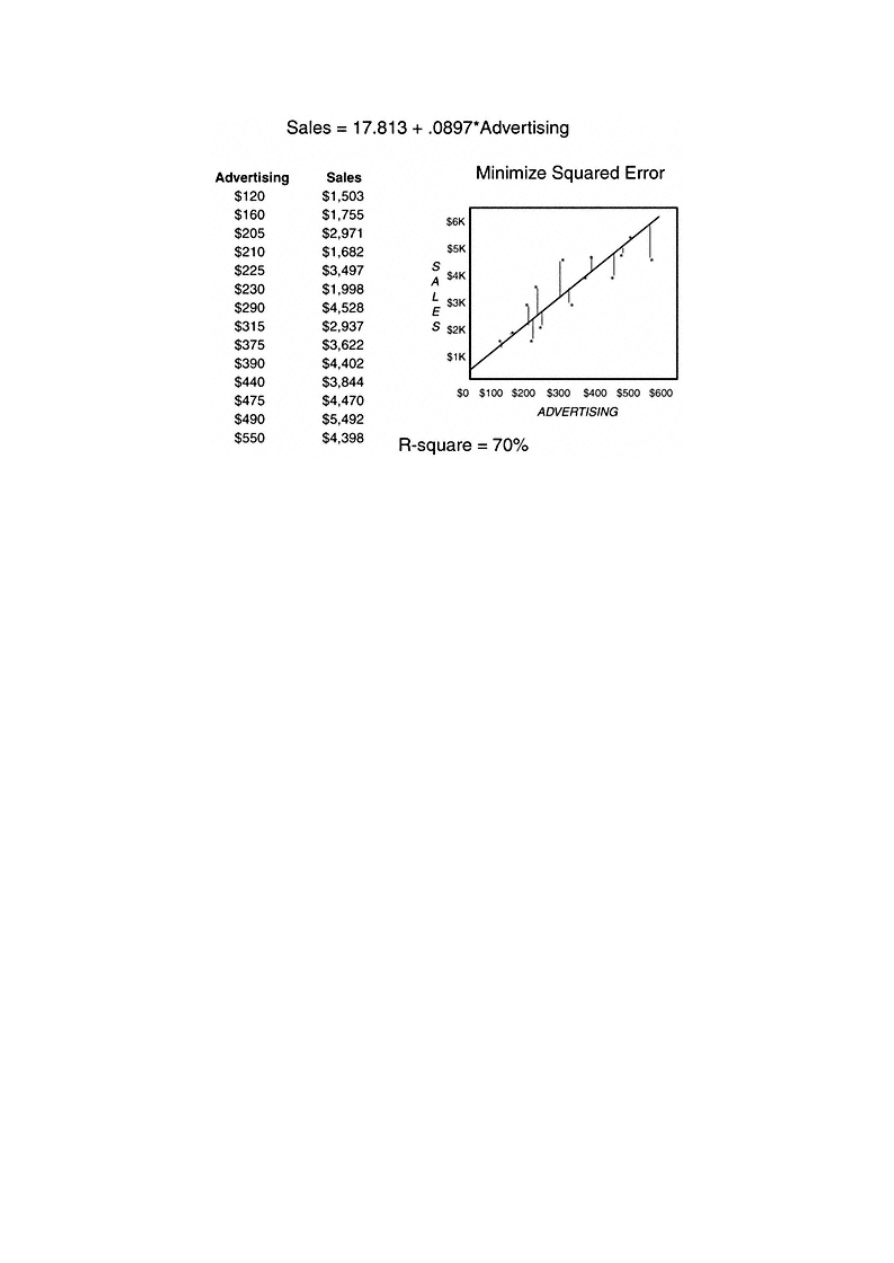
Page 13

Figure

1.2

Simple

linear

regression— linear

relationship.

ship is the R-square. The R-square measures the amount of the overall variation in the data that is explained by the
model. This regression analysis results in an R-square of 70%. This implies that 70% of the variation in sales can be
explained by the variation in advertising.

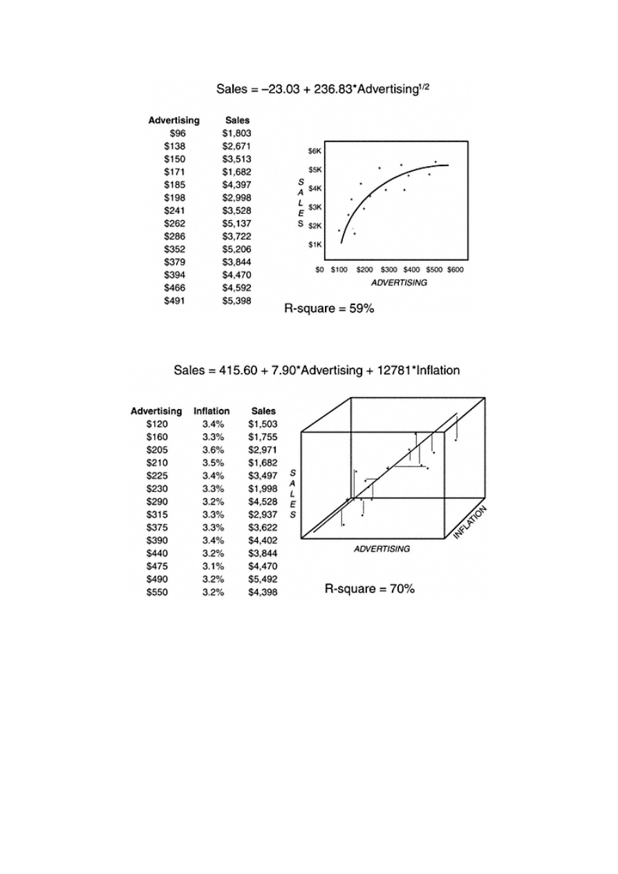
Sometimes the relationship between the dependent and independent variables is not linear. In this situation, it may be
necessary to transform the independent or predictive variable to allow for a better fit. Figure 1.3 shows a curvilinear
relationship between sales and advertising. By using the square root of advertising we are able to find a better fit for the
data.

When building targeting models for marketing, risk, and customer relationship management, it is common to have many
predictive variables. Some analysts begin with literally thousands of variables. Using multiple predictive or independent
continuous variables to predict a single continuous variable is called multiple linear regression. In Figure 1.4,
advertising dollars and the inflation rate are linearly correlated with sales.

Targeting models created using linear regression are generally very robust. In marketing, they can be used alone or in
combination with other models. In chapter 12 I demonstrate the use of linear regression as part of the lifetime value
calculation.

Team-Fly

Page 14

Figure

1.3

Simple

linear

regression— curvilinear

relationship.

Figure

1.4

Multiple

linear

regression.ting

the

Objective

Page 15

Logistic Regression

Logistic regression is very similar to linear regression. The key difference is that the dependent variable is not
continuous; it is discrete or categorical. This makes it very useful in marketing because we are often trying to predict a
discrete action such as a response to an offer or a default on a loan.

Technically, logistic regression can be used to predict outcomes for two or more levels. When building targeting models
for marketing, however, the outcome usually has a two-level outcome. In order to use regression, the dependent variable
is transformed into a continuous value that is a function of the probability of the event occurring.

My goal in this section is to avoid heavy statistical jargon. But because this is the primary method used in the book, I am
including a thorough explanation of the methodology. Keep in mind that it is very similar to linear regression in the
actual model processing.

In Figure 1.5, the graph displays a relationship between response (0/1) and income in dollars. The goal is to predict the
probability of response to a catalog that sells high-end gifts using the prospect's income. Notice how the data points have
a value of 0 or 1 for response. And on the income axis, the values of 0 for response are clustered around the lower values
for income. Conversely, the values of 1 for response are clustered around the higher values for income. The sigmoidal
function or s-curve is formed by averaging the 0s and 1s for each

Figure

1.5

Logistic

regression.

Page 16

value of income. It is simple to see that higher-income prospects respond at a higher rate than lower -income prospects.

The processing is as follows:

1. For each value of income, a probability (p) is calculated by averaging the values of
response.

2. For each value of income, the odds are calculated using the formula p/(1–p) where p is the probability.

3. The final transformation calculates the log of the odds: log(p/(1–p)).

The model is derived by finding the linear relationship of income to the log of the odds using the equation:

where

are the coefficients and X

. X

are the predictive variables. Once the predictive coefficients or weights

(

s) are derived, the final probability is calculated using the following formula:

This formula can also be written in a simpler form as follows:

Similar to linear regression, logistic regression is based on a statistical distribution. Therefore it enjoys the same benefits
as linear regression as a robust tool for developing targeting models.

Neural Networks

Neural network processing is very different from regression in that it does not follow any statistical distribution. It is
modeled after the function of the human brain. The process is one of pattern recognition and error minimization. You
can think of it as taking in information and learning from each experience.

Neural networks are made up of nodes that are arranged in layers. This construction varies depending on the type and
complexity of the neural network. Figure 1.6 illustrates a simple neural network with one hidden layer. Before the
process begins, the data is split into training and testing data sets. (A third group is held out for final validation.) Then
weights or ''inputs" are assigned to each of the nodes in the first layer. During each iteration, the inputs are processed
through the system and compared to the actual value. The error is measured and fed back through the system to adjust
the weights. In most cases,

Page 17

Figure

1.6

Neural

network.

the weights get better at predicting the actual values. The process ends when a predetermined minimum error level is
reached.

One specific type of neural network commonly used in marketing uses sigmoidal functions to fit each node. Recall that
this is the same function that is used in logistic regression. You might think about this type of neural network as a series
of "nested" logistic regressions. This technique is very powerful in fitting a binary or two -level outcome such as a
response to an offer or a default on a loan.

One of the advantages of a neural network is its ability to pick up nonlinear relationships in the data. This can allow
users to fit some types of data that would be difficult to fit using regression. One drawback, however, is its tendency to
over-fit the data. This can cause the model to deteriorate more quickly when applied to new data. If this is the method of
choice, be sure to validate carefully. Another disadvantage to consider is that the results of a neural network are often
difficult to interpret.

Genetic Algorithms

Similar to neural networks, genetic algorithms do not have an underlying distribution. Their name stems from the fact
that they follow the evolutionary

Page 18

process of "survival of the fittest." Simply put, many models are compared and adjusted over a series of iterations to find
the best model for the task. There is some variation among methods. In general, though, the models are altered in each
step using mating, mutation, and cloning.

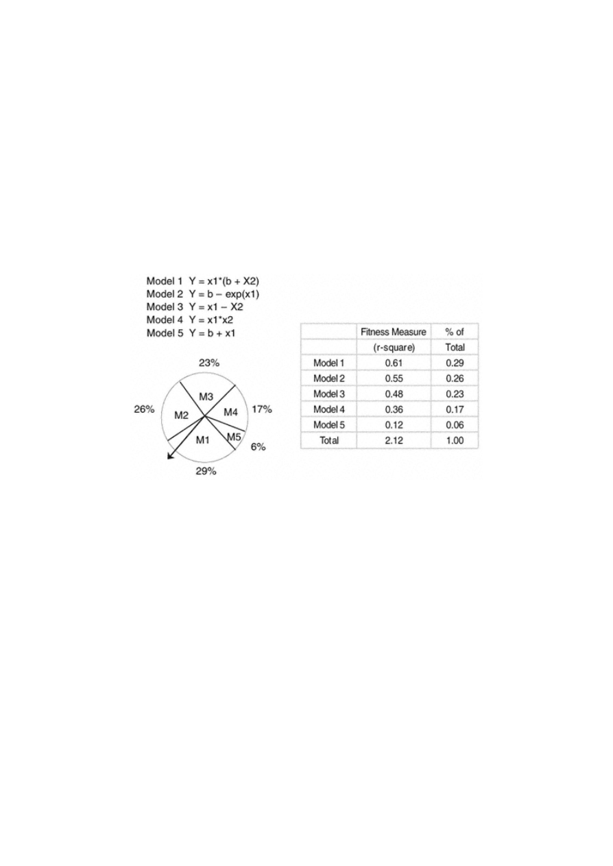
As with all modeling methods, the first step is to determine the objective or goal of the model. Then a measure is
selected to evaluate model fit. Let's say we want to find the best model for predicting balances. We use R-square to
determine the model fit. In Figure 1.7 we have a group of models that represent the "first generation" of candidate
models. These were selected at random or created using another technique. Each model is tested for its ability to predict
balances. It is assigned a value or weight that reflects its ability to predict balances in comparison to its competitors. In
the right-hand column, we see that the "% of Total" is calculated by dividing the individual R -square by the sum of the
R-squares. This "% of Total" is treated like a weight that is then used to increase or decrease the model's chances to
survive in the next generation of tests. In addition to the weights, the models are randomly subjected to other changes
such as mating, mutation, and cloning. These involve randomly switching variables, signs, and functions. To control the
process, it is necessary to establish rules for each process. After many iterations, or generations, a winning model will
emerge. It does an excellent job of fitting a model. It, however, requires a lot of computer power. As computers continue
to become more powerful, this method should gain popularity.

Figure

1.7

Genetic

algorithms.

Page 19

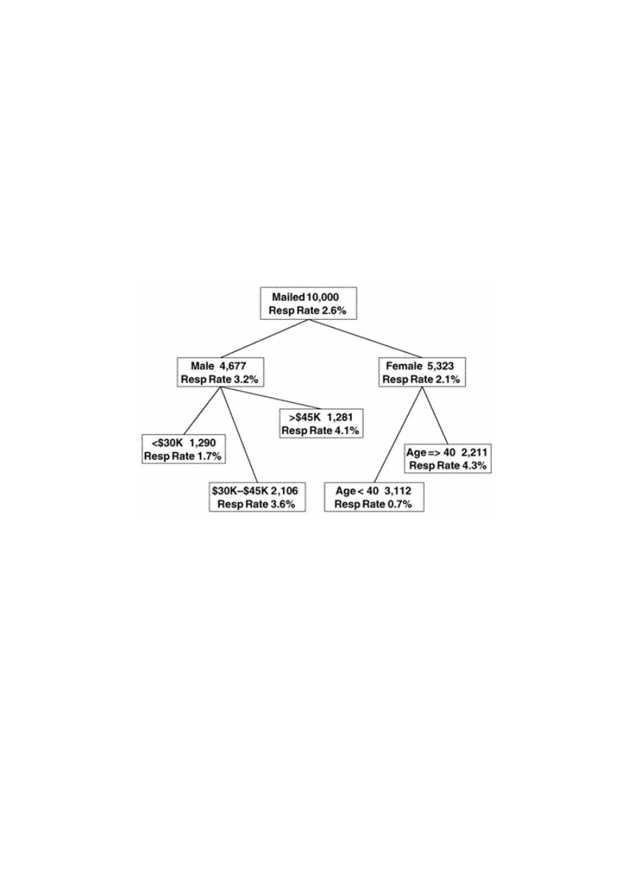
Classification Trees

The goal of a classification tree is to sequentially partition the data to maximize the differences in the dependent
variable. It is often referred to as a decision tree. The true purpose of a classification tree is to classify the data into
distinct groups or branches that create the strongest separation in the values of the dependent variable.

Classification trees are very good at identifying segments with a desired behavior such as response or activation. This
identification can be quite useful when a company is trying to understand what is driving market behavior. It also has an
advantage over regression in its ability to detect nonlinear relationships. This can be very useful in identifying
interactions for inputs into other modeling techniques. I demonstrate this in chapter 4.

Classification trees are "grown" through a series of steps and rules that offer great flexibility. In Figure 1.8, the tree
differentiates between responders and nonresponders. The top node represents the performance of the overall campaign.
Sales pieces were mailed to 10,000 names and yielded a response rate of 2.6%. The first split is on gender. This implies
that the greatest difference between responders and nonresponders is gender. We see that males are much more
responsive (3.2%) than females (2.1%). If we stop after one split, we would

Figure

1.8

Classification

tree

for

response.

Page 20

consider males the better target group. Our goal, though, is to find groups within both genders that discriminate between
responders and nonresponders. In the next split, these two groups or nodes are considered separately.

The second-level split from the male node is on income. This implies that income level varies the most between
responders and nonresponders among the males . For females, the greatest difference is among age groups. It is very easy
to identify the groups with the highest response rates. Let's say that management decides to mail only to groups where
the response rate is more than 3.5%. The offers would be directed to males who make more than $30,000 a year and
females over age 40.

A definite advantage of classification trees over other techniques is their ability to explain the results. I often develop
complex logistic models for scoring and build a tree to explain the results to the marketers. Although the outcome is
never identical, the tree does a good job of uncovering key drivers in the market. Due to their broad applicability,
classification trees will continue to be a valuable tool for all types of target modeling.

The Adaptive Company

Every year more companies are embracing analytics to help them improve their marketing efforts. Doing so is no longer
a luxury. The analytic approach to marketing is necessary for survival. There are many challenges in making a
successful transition, however. One of the biggest challenges is being able to adapt quickly to change.

This is one situation in which smaller, leaner companies often have an advantage. Because adapting often requires total
company realignment, some older, larger companies find it difficult to embrace the analytic approach for several
reasons. First, their data systems don't support the information needs of the new paradigm. Second, the decision makers
often don't understand the sophisticated technologies required to drive the business. This can make them resistant to
using them. And third, the company personnel and compensation structures aren't designed to support the new approach.

The companies that are leading the pack are those that have managers and senior executives who support an analytic
approach to marketing, risk, and customer relationship management. So many facets of the organizational structure need
to be aligned to make it work. And all levels of management must agree to the goal and understand the ramifications.
Consider the credit card bank whose management team was frustrated with their low approval rates. They asked the
analytic group to build an acquisition model that targeted more

Page 21

approvable responders. The model was successfully developed with the caveat that response rates would decline
slightly. But the overall number of accounts per piece mailed would be higher, leading to higher profits per piece mailed.
Management approved the model-building project. When the model was implemented and response rates dropped,
though, panic set in and the model was withdrawn from use.

To be successful, every area of the company must be willing to work toward the same goals. The finance department
must be willing to work with other areas of the company to align revenue and profitability measures. The information
technology group must support the hardware, software, and data needs of the analysts. The employees involved in the
day-to-day production of goods and services must be willing to support the analytic approach by providing information
and incorporating procedures to facilitate the flow of information. And finally, if the company has made a commitment
to support an analytic approach, the rewards and incentives for all employees must be aligned with that commitment.

Hiring and Teamwork

Hiring talented analysts is key to the success of this approach. Human resources personnel must be trained to understand
and identify the skills and education necessary to succeed in highly technical positions. Jerry Bernhart, of Bernhart and
Associates, shares his insights in hiring a good market analyst:

It has been my experience that in recruiting the best quantitative analysts it is not enough for them to know just the
statistical tools. They must know how to apply them to real-world marketing problems. A hammer is a hammer, but the best
carpenters know how to swing it. There is a big difference between the number cruncher who understands it from a
textbook perspective and the true market analyst who can interpret it and apply it to the business.

When interviewing junior-level candidates with little or no on-the-job experience in research or analysis you certainly can't
expect them to give you a treatise on strategic marketing. However, you can use scenario-driven interviewing to reveal
whether or not they have at least an intuitive understanding of what it means to solve a marketing problem.

Once you hire them, keep them challenged. When you ask what motivates a market analyst, money is rarely at the top of the
list. Rather, what you'll hear most often is that they want an opportunity where they can learn and apply new analytical
methodologies. Good analysts tend to be highly creative, always looking for better ways to solve problems.

I totally concur with Jerry's views. The basic knowledge is important, but the breakthroughs come from the analyst's
ability to creatively blend and adapt the latest tools and techniques.

Page 22

Once you hire a good analyst, retaining him or her can be a challenge. The marketplace has many opportunities for this
type of talent. As Jerry said, money is rarely a top motivator. So here are a few tips for managers: Give your analysts
opportunities to learn and expand their skill base, supply them with leading-edge hardware and software, create
opportunities for challenge and variety, and offer them flexible hours and workplace options. Jodi Barnes Nelson, Ph.D.,
a professor of Human Resources at North Carolina State University, comments on the organizational structure of the
future:

The virtual organization is quickly becoming a reality. We saw this in academia in the late 1980s with the wide acceptance
of e-mail and listservs. Researchers in far-reaching places could now participate in joint projects with colleagues. As
organizations down-size, rightsize, and globalize, the boundary-less organization becomes a reality.

Finally, management must encourage teamwork and develop leadership incentives to meet the company goals. For
example, if the company decides that attracting profitable customers is the primary goal, accountability and incentives
need to be assigned to promote that goal. Consider the credit card bank that wanted to attract new profitable customers.
The analyst developed a targeting model that attracted customers who were likely to build balances and retain those
balances. When responses came in and it was time to approve the account, the risk department stepped in and declined
the prospects with the greatest profit potential. Why? Because they had a risk level that was unacceptable. And the risk
department was not striving for profitable customers; it was simply tasked with managing risk. So the risk department
did not consider the fact that the higher-risk customers were much more likely to maintain balances at higher rates,
thereby making them much more profitable.

Product Focus versus Customer Focus

As mentioned earlier, many companies are making the transition from a product focus to a customer focus. The reason
for this transition is simple: In many industries it is becoming more difficult to attract new customers. It has become
more efficient to broaden the company focus and develop new products for existing customers. This evolution from a
product focus to a customer focus has been a gradual process. Mark Van Clieaf, Managing Director of MVC Associates
International, details the history of this transition:

Marketing decision sciences have played a role in each of "three waves" of becoming customer centric over the last 15
years. First came the loyalty/frequency wave. This started with many of the continuity clubs (books, music), airlines, and
catalog companies. Initially good information-based marketing differentiated customers based on

Barnes Nelson, J., Ph.D. 1997. "The Boundaryless Organization: Implications for Job Analysis, Recruitment and

Selection." Human Resources Planning 20(4):39–49.

Page 23

simple RFM metrics (recency, frequency, monetary value). Many loyalty programs were developed to attempt to recognize,
differentiate, and reward tiers of better customers.

The second wave, customer value optimization, aimed for more precise matching of product to customer, with some level of
tailoring products and services to smaller niches of customer segments. Where the first and second waves were essentially
about products in search of customers, the third wave starts with customers and what can be done to meet their needs with
products and services, whether individually or bundled. The third wave has seen a select few companies begin to use
marketing decision sciences to create a single customer view across multiple product categories or lines of business. This
customer view also includes the duration of the relationship beyond the one-year profit-and-loss statement and the financial
implications for optimizing pricing and marketing spending over multiple years. This single view allows for the creation of
new bundled value propositions.

One of the most difficult aspects of this transition has been from the "silo" structure where each manager owns a product
to a market-based structure where each manager is responsible for a share of the market. If a company is expanding its
products and services, the customer focus becomes critically important. Consider the company that relied heavily on its
current customers for increased sales. Its new customer acquisition efforts were only marginally successful. So the
company met its annual revenue goals by cross-selling and up-selling its current customers. Because each manager was
responsible for a single product, all the managers were soliciting the same customers. Soon the customers started
complaining about the number of telemarketing calls they were receiving. Many cancelled their accounts. One incident
was reported where a customer had two solicitors from different divisions of the same company on the phone at the
same time (using call waiting). On further analysis, it was determined that the customers deemed the most profitable
were receiving as many as 30 calls a month. In essence, the company was abusing its best customers. The company was
finally motivated to adopt a customer value approach to marketing that evaluated every offer based on a total customer
value proposition.

Summary

As we move into the chapters ahead, we will become immersed in the intricate steps involved in developing targeting
models. Remember to stay focused on the overall goal of the project. At every step, you should evaluate whether the
process is continuing to meet your goals. And keep in mind that the successful company is able to adapt to the rapid
changes in technology and market dynamics with ease. This success is made possible by a team of talented analysts who

Team-Fly

Page 24

receive the respect and company support necessary to contribute creatively and effectively.

Once you have defined your objective and chosen the methodology, the next step is to determine the best source of data
for the analysis. In the next chapter, I discuss the foundation of good analysis — the data. I will describe many types of
data along with some typical sources and uses. I use multiple examples to describe some typical data sources for
marketing, risk, and customer relationship management.

Page 25

Chapter 2—
Selecting the Data Sources

The world of data mining is experiencing an information explosion. The amount and complexity of data are expanding.
And as companies embrace Web sites as a marketing and CRM tool, the amount of data is increasing exponentially.

To enhance their data mining efforts, many companies are diligently collecting, combining, and scrubbing data.
Companies new to data mining are revamping their databases to allow for easier access and extractability. Companies
whose primary business is to collect, enhance, and sell data are springing up every day. All of this can be a bit
overwhelming. So, in this chapter, I start at the beginning. The first step in making the best use of any data source is to
understand the nature of the data as well as how it is gathered and managed.

Chapter 2 begins with a discussion of various types of data along with the strengths and weakness of each type. The next
section discusses some typical data sources with descriptions and cases from both internal and external repositories. The
final section of the chapter offers some ideas for creating targeting model data sets; this section also includes numerous
case studies. To create your own targeting model data set, you can use the definitions and case studies in this chapter as
a template, creatively modifying these cases to develop a customized fit for your unique objective.

Page 26

Types of Data

No matter where it comes from, data falls into three basic types: demographic, behavioral, and psychographic or
attitudinal. Each type has its strengths and weaknesses.

Demographic data generally describes personal or household characteristics. It includes characteristics such as
gender, age, marital status, income, home ownership, dwelling type, education level, ethnicity, and presence of children.
Demographic data has a number of strengths. It is very stable, which makes it appealing for use in predictive modeling.
Characteristics like marital status, home ownership, education level, and dwelling type aren't subject to change as
frequently as behavioral data such as bank balances or attitudinal characteristics like favorite political candidate. And
demographic data is usually less expensive than attitudinal and behavioral data, especially when purchased on a group
level. One of the weaknesses of demographic data is that it is difficult to get on an individual basis with a high degree of
accuracy. Unless it is required in return for a product or service, many people resist sharing this type of information or
supply false information.

Behavioral data is a measurement of an action or behavior. Behavioral data is typically the most predictive type of
data. Depending on the industry, this type of data may include elements like sales amounts, types and dates of purchase,
payment dates and amounts, customer service activities, insurance claims or bankruptcy behavior, and more. Web site
activity is another type of behavioral data. A Web site can be designed to capture sales as well as click stream behavior
or the exact path of each Web site visitor.

Behavioral data usually does a better job of predicting future behavior than the other types of data. It is, however,
generally the most difficult and expensive data to get from an outside source. This will be discussed in more detail
in the next section.

Psychographic or attitudinal data is characterized by opinions, lifestyle characteristics, or personal values.
Traditionally associated with market research, this type of data is mainly collected through surveys, opinion polls, and
focus groups. It can also be inferred through magazine and purchase behavior. Due to increased competition, this type of
data is being integrated into customer and prospect databases for improved target modeling and analysis.

Psychographic data brings an added dimension to predictive modeling. For companies that have squeezed all the
predictive power out of their demographic and behavioral data, psychographic data can offer some improve-

Page 27

ment. It is also useful for determining the life stage of a customer or prospect. This creates many opportunities for
developing products and services around life events such as marriage, childbirth, college, and retirement.

The biggest drawback to psychographic data is that it denotes intended behavior that may be highly, partly, or
marginally correlated with actual behavior. Data may be collected through surveys or focus groups and then applied
to a larger group of names using segmentation or another statistical technique. If data is applied using these
methods, it is recommended that a test be constructed to validate the correlation.

Table 2.1 provides a quick reference and comparison of the three main types of data. The rating is based on individual-
level data. If data is collected on a group and inferred on an individual level, it is generally less predictive and less
expensive. The stability is about the same.

Table 2.1 Data Types and Characteristics

PREDICTIVE POWER

STABILITY

COST

Demographic

Medium

High

Low

Behavioral

High

Low

High

Psychographic

Medium

High

Sources of Data

Data for modeling can be generated from a number of sources. Those sources fall into one of two categories: internal or
external. Internal sources are those that are generated through company activity such as customer records, Web site, mail
tapes from mail or phone campaigns, or databases and/or data warehouses that are specifically designed to house
company data. External sources of data include companies such as the credit bureaus, list brokers and compilers, and
corporations with large customer databases like publishers and catalogers.

Internal Sources

Internal sources are data sources that are housed within a company or establishment. They are often the most predictive
data for modeling because they represent information that is specific to the company's product or service.

Page 28

Some typical sources are the customer database, transaction database, offer history database, solicitation tapes, and data
warehouses. The next section details the typical features and components of those databases.

Customer Database

A customer database is typically designed with one record per customer. In some organizations, it may be the only
database. If that is the case, it may contain all the sales and/or activity records for every customer. It is more common,
though, that the customer database contains the identifying information that can be linked to other databases such as a
transaction database to obtain a current snapshot of a customer's performance. Even though there may be wide variation
among companies and industries, the following list details some key elements in a typical customer database:

Customer ID. A unique numeric or alphanumeric code that identifies the customer throughout his or her entire
lifecycle. Some companies may use an account number for this function, but this can be risky if the account numbers are
subject to change. For example, credit card banks assign a new account number when a card is lost or stolen. The
customer ID allows each account number to be linked to the unique customer, thereby preserving the entire customer
history. It is essential in any database to effectively link and tract the behavior of and actions taken on an individual
customer.

Household ID. A unique numeric or alphanumeric code that identifies the household of the customer through his or her
entire lifecycle. This identifier is useful in some industries where more than one member of a household shares products
or services.

Account number. A unique numeric or alphanumeric code that relates to a particular product or service. One customer
can have several account numbers.

Customer name. The name of a person or a business. It is usually broken down into multiple fields: last name, first
name, middle name or initial, salutation.

Address. The street address, typically broken into components such as number, street, suite or apartment number, city,
state, and zip + 4. Some customer databases have a line for a P.O. Box. With population mobility about 10% per year,
additional fields that contain former addresses are useful for tracking and matching customers to other files.

Phone number. Current and former numbers for home and work.

Demographics. Characteristics such as gender, age, and income may be stored for profiling and modeling.

Page 29

Products or services. The list of products and product identification numbers that varies by company. An insurance
company may list all the policies along with policy numbers. A bank may list all the products across different divisions
of the bank including checking, savings, credit cards, investments, loans, and more. If the number of products and the
product detail are extensive, this information may be stored in a separate database with a customer and household
identifier.

Offer detail. The date, type of offer, creative, source code, pricing, distribution channel (mail, telemarketing, sales rep,
e-mail), and any other details of an offer. Most companies look for opportunities to cross-sell or up -sell their current
customers. There could be numerous ''offer detail" fields in a customer record, each representing an offer for an
additional product or service.

Model scores. Response, risk, attrition, profitability, scores, and/or any other scores that are created or purchased.

Transaction Database

The transaction database contains records of customer activity. It is often the richest and most predictive information,
but it can be the most difficult to utilize. In most cases, each record represents a single transaction, so there may be
multiple records for each customer. The transaction database can take on various forms depending on the type of
business. In order to use this data for modeling, it must be summarized and aggregated to a customer level. Number of
records per customer can differ. The following list is typical of what might be found in a transaction database:

Customer ID. A unique numeric or alphanumeric code that identifies the customer throughout his or her entire
lifecycle. Some companies may use an account number for this function.

Account number. A unique numeric or alphanumeric code that relates to a particular product or service.

Sales activity. The amount of the transaction.

Date of activity. Date the transaction occurred.

A credit card transaction database will typically contain dates, charge amounts, returns, payments, and fee activity
including late fees, overlimit fees, and/or annual fees. A useful summarization for modeling is monthly totals for each
field. A catalog company's transaction database will typically contain dates, source codes that identify the specific
catalog, sales, and returns.

Page 30

Offer History Database

The offer history database contains details about offers made to prospects, customers, or both. The most useful format is
a unique record for each customer or prospect. Variables created from this database are often the most predictive in
response and activation targeting models. It seems logical that if you know someone has received your offer every
month for six months, they are less likely to respond than someone who is seeing your offer for the first time. As
competition intensifies, this type of information is becoming increasing important.

A customer offer history database would contain all cross-sell, up-sell, and retention offers. A prospect offer history
database would contain all acquisition offers as well as any predictive information from outside sources. It is also useful
to store former addresses on the prospect offer history database.

TIP

It is common to purchase prospect data repeatedly from the same source. The goal may
be to purchase new names or to get fresh information about existing names. In either
case, it is useful to arrange with the data seller to assign a unique identifier to each
prospect that is housed on the seller's database. Then when additional names are
purchased or current names are refreshed, the match rate is much higher.

With an average amount of solicitation activity, this type of database can become very large. It is important to perform
analysis to establish business rules that control the maintenance of this database. Fields like "date of first offer" are
usually correlated with response behavior. The following list details some key elements in an offer history database:

Prospect ID/customer ID. A unique numeric or alphanumeric code that identifies the prospect for a specific length of
time.

Prospect name.

The name of a person or a business. It is usually broken down into multiple fields: last name, first

name, middle name or initial, salutation.

Address.

The street address, typically broken into components such as number, street, suite or apartment number, city,

state, zip + 4. As in the customer database, some prospect databases have a line for a P.O. Box.

These elements appear only on a prospect offer history database. The customer database would support the customer offer

history database with additional data.

Page 31

Additional fields that contain former addresses are useful for matching prospects to outside files.

Phone number. Current and former numbers for home and work.

Offer detail. Includes the date, type of offer, creative, source code, pricing, distribution channel (mail, telemarketing,
sales rep, e-mail), and any other details of the offer. There could be numerous groups of "offer detail" fields in a
prospect or customer record, each representing an offer for an additional product or service.

Offer summary. Date of first offer (for each offer type), best offer (unique to product or service), etc.

Model scores.

Response, risk, attrition, profitability scores, and/or any other scores that are created or purchased.

Predictive data.

Includes any demographic, psychographic, or behavioral data.

Solicitation Mail and Phone Tapes

Solicitation tapes are created from either a customer database or a prospect list to provide pertinent information for a
campaign. The tapes are usually shipped to a processor for mailing or a telemarketing shop for phone offers. If the goal
is to eventually build a model from a specific campaign, the solicitation tape should contain the following information:

Customer or prospect ID. Described previously, this field can be used to match back to the customer or prospect
database.

Predictive data. If data is purchased from an outside list company for the purpose of building a model, the predictive
data for model development is included on the solicitation tape.

Data Warehouse

A data warehouse is a structure that links information from two or more databases. Using the data sources mentioned in
the previous section, a data warehouse brings the data into a central repository, performs some data integration, clean-
up, and summarization, and distributes the information data marts. Data marts are used to house subsets of the data from
the central repository that has been selected and prepared for specific end users. (They are often called departmental data
warehouses.) An analyst who wants to get data for a targeting model accesses the relevant data mart. The meta data
provides a directory for the data marts. Figure 2.1 shows how the data gets from the various data sources, through the
central repository to the data marts.

Page 32

Figure 2.1 displays just one form of a data warehouse. Another business might choose an entirely different structure.
The purpose of this section is to illustrate the importance of the data warehouse as it relates to accessing data for
targeting model development.

Drury Jenkins, an expert in business intelligence systems, talks about the data warehouse and how it supports business
intelligence with special emphasis on modeling and analytics:

Business intelligence is the corporate ability to make better decisions faster. A customer-focused business intelligence
environment provides the infrastructure that delivers information and decisions necessary to maximize the most critical of
all corporate assets— the customer base. This infrastructure combines data, channels, and analytical techniques to enhance
customer satisfaction and profitability through all major customer contact points. For marketers this means the ability to
target the right customer, at the right time, in the right place, and with the right product. The channels include traditional as
well as the fast-growing electronic inbound and outbound. The analytical techniques include behavior analysis, predictive
modeling, time-series analysis, and other techniques.

The key aspect to supplying the necessary data is the creation of a total view for each individual customer and their needs.
Integration of customer data must provide a single, unified and accurate view of their customers across the entire
organization. The

Figure

2.1

typical

data

warehouse.electing

the

Data

Sources

Page 33

ultimate goal is to achieve a complete picture of a customer's interaction with the entire organization, only achieved by
gathering and staging the appropriate data. In addition to pulling in demographics and other external data, numerous internal
data are necessary.

Too often, obtainable data are fragmented and scattered over multiple computer sites and systems, hidden away in
transaction database systems or personal productivity tools such as spreadsheets or micro databases. These disparate data
were created in the most part by the explosive growth of client/server applications over the last decade, creating
independent transaction-oriented databases. Implementing independent On Line Transaction Processing (OLTP) customer
contact point systems, as opposed to an integrated Customer Relationship Management (CRM) approach, has also added to
the disparate data problems. These customer service, sales force automation, call center, telesales, and marketing
applications look at customers from different views, making it difficult to create a holistic view of the customer.

Identifying what data are needed for the customer-focused environment should begin with business drivers. It should end
with innovative thinking about what information is needed and how it can be used to increase your customer base and
loyalty. Once the data elements and usage are identified, a business intelligence architecture must exist that supports the
necessary infrastructure. The most simplistic way to look at business intelligence architecture is by three segments:

• Gathering the important data

• Discovering and analyzing data while transforming to pertinent information

• Delivering the information

The second segment refers to analyzing data about customers and prospects through data mining and model development.
The third segment also includes data analysis along with other information exploitation techniques that deliver information
to employees, customers, and partners. The most misunderstood segment is probably the first, gathering the important data.

Numerous terms are used to describe the data gathering and storing aspect of a business intelligence environment. The
primary term, data warehousing, has a metamorphosis of its own. Then we add in terms like data mart, central repository,
meta data, and others. The most important data repository aspect is not its form, but instead the controls that exist. Business
intelligence infrastructure should consist of the following control components:

• Extracting and staging data from sources

• Cleaning and aligning data/exception handling

• Transporting and loading data

• Summarizing data

• Refreshing process and procedures

• Employing meta data and business rules

Team-Fly

Page 34

The first five activities involve pulling, preparing, and loading data. These are important and must be a standard and
repeatable process, but what is the role of meta data?

• Central control repository for all databases

• Repository for data hierarchies

• Repository for data rules, editing, transformations

• Repository for entity and dimension reference data

• Optimizes queries

• Common business definitions

• Hides complexity

• Links legacy systems to the warehouse repositories

• User and application profiling

There are two types of meta data— system and business. System meta data states the sources, refresh date, transformations,
and other mechanical controls. Business meta data is used by analysts to understand where data is found as well as
definitions, ownership, last update, calculations, and other rule-based controls. It is easy to see the importance of meta data
to the business intelligence environment.

Data Warehousing: Mistakes and Best Practices

Drury also shares some common data warehousing mistakes, keys to success, and industry "best
practices."

What are some of the common data warehousing mistakes?

•

Not implementing a comprehensive meta data strategy

•

Not deploying a centralized warehouse administration tool

•

Not cleaning or intergrating transactional data

•

Expecting the warehouse to stay static

•

Underestimating refresh and update cycles

•

Using a poor definition and approach

•

Poor design and data modeling

•

Using inexperienced personnel

Page 35

There are a lot of data warehouse horror stories; however, there are also a lot of phenomenal success
stories. What are the keys to a successful implementation?

•

Executive sponsorship is a must.

•

A full-time project team with experienced staff is necessary.

•

Both IT and business units must be involved in the project.

•

Business analysts who understand the business objective as well as the data warehouse and the data mining

technology must be involved.

•

The project's scope must be focused and achievable.

•

Activities must support the business goals.

•

An iterative approach must be used to build, test, and implement the solution.

•

Proven technology components must be used.

•

Data quality is a priority.

•

Think globally. Act locally.

•

Implement short term. Plan long term.

Now let's look at some data warehousing "Best Practices":

•

Transactional systems flow up to a consolidating layer where cleansing, integration, and alignment occur.

This Operational Data Store (ODS) layer feeds a dimensionally modeled data warehouse, which typically
feeds application or departmentalized data marts.

•

Data definitions are consistent, data is cleaned, and a clear understanding of a single system of record

exists— "one version of the truth."

•

Meta data standards and systems are deployed to ease the change process. All new systems are meta data

driven for cost, speed, and flexibility.

•

Technology complexity of databases is hidden by catalog structures. Clean interfaces to standard desktop

productivity tools. Self-service is set up for end users with business meta data, so they can get their own data
with easy-to -use tools.

As in data mining and model development, building and implementing a data warehouse require careful planning,
dedicated personnel, and full company support. A well-designed data warehouse provides efficient access to multiple
sources of internal data.

Page 36

External Sources

The pressure is on for many companies to increase profits either through acquiring new customers or by increasing sales
to existing customers. Both of these initiatives can be enhanced through the use of external sources.

External sources consist mainly of list sellers and compilers. As you would expect, list sellers are companies that sell
lists. Few companies, however, have the sale of lists as their sole business. Many companies have a main business like
magazine sales or catalog sales, with list sales as a secondary business. Depending on the type of business, they usually
collect and sell names, addresses, and phone numbers, along with demographic, behavioral, and/or psychographic
information. Sometimes they perform list "hygiene" or clean-up to improve the value of the list. Many of them sell their
lists through list compilers and/or list brokers.

List compilers are companies that sell a variety of single and compiled lists. Some companies begin with a base like the
phone book or driver's license registration data. Then they purchase lists, merge them together, and impute missing
values. Many list compliers use survey research to enhance and validate their lists.

There are many companies that sell lists of names along with contact information and personal characteristics. Some
specialize in certain types of data. The credit bureaus are well known for selling credit behavior data. They serve
financial institutions by gathering and sharing credit behavior data among their members. There are literally hundreds of
companies selling lists from very specific to nationwide coverage. (For information regarding specific companies, go to

http://dataminingcookbook.wiley.com

Selecting Data for Modeling

Selecting the best data for targeting model development requires a thorough understanding of the market and the
objective. Although the tools are important, the data serves as the frame or information base. The model is only as good
and relevant as the underlying data.

Securing the data might involve extracting data from existing sources or developing your own. The appropriate selection
of data for the development and validation of a targeting model is key to the model's success. This section describes
some of the different sources and provides numerous cases from a variety of industries. These cases are typical of those
used in the industry for building targeting models.

Page 37

The first type of data discussed in this section is prospect data. This data is used for prospecting or acquiring new
customers. For most companies this task is expensive, so an effective model can generate considerable savings. Next I
discuss customer data. This data is used to cross-sell, up -sell, and retain existing customers. And finally, I discuss
several types of risk data. This is appropriate for both prospects and customers.

Data for Prospecting

Data from a prior campaign is the best choice for target modeling. This is true whether or not the prior campaign
matches the exact product or service you are modeling. Campaigns that have been generated from your company will be
sensitive to factors like creative and brand identity. This may have a subtle effect on model performance.

If data from a prior campaign is not available, the next best thing to do is build a propensity model. This modeling
technique takes data from an outside source to develop a model that targets a product or service similar to your primary
targeting goal.

TIP

For best results in model development, strive to have the population from which the data
is extracted be representative of the population to be scored.

More and more companies are forming affinity relationships with other companies to pool resources and increase
profits. Credit card banks are forming partnerships with airlines, universities, clubs, retailers, and many others.
Telecommunications companies are forming alliances with airlines, insurance companies, and others. One of the
primary benefits is access to personal information that can be used to develop targeting models.

Modeling for New Customer Acquisition

Data from a prior campaign for the same product and to the same group is the optimal choice for data in any targeting
model. This allows for the most accurate prediction of future behavior. The only factors that can't be captured in this
scenario are seasonality, changes in the marketplace, and the effects of multiple offers. (Certain validation methods,
discussed in chapter 6, are designed to help control for these time-related issues.)

As I mentioned earlier, there are a many ways to create a data set for modeling. But many of them have similar
characteristics. The following cases are designed to provide you with ideas for creating your own modeling data sets.

Page 38

Case 1—
Same Product to the Same List Using a Prior Campaign

Last quarter, ABC Credit Card Bank purchased approximately 2 million names from Quality Credit Bureau for an
acquisition campaign. The initial screening ensured that the names passed ABC's minimum risk criteria. Along with the
names, ABC purchased more than 300 demographic and credit attributes. It mailed an offer of credit to the entire list of
names with an annualized percentage rate (APR) of 11.9% and no annual fee. As long as all payments are received
before the monthly due date, the rate is guaranteed not to change for one year. ABC captured the response from those
campaigns over the next eight weeks. The response activity was appended to the original mail tape to create a modeling
data set.

Over the next four weeks, ABC Credit Card Bank plans to build a response model using the 300+ variables that were
purchased at the time of the original offer. Once the model is constructed and validated, ABC Credit Card Bank will
have a robust tool for scoring a new set of names for credit card acquisition. For best results, the prospect should be sent
the same offer (11.9% APR with no annual fee) using the same creative. In addition, they should be purchased from
Quality Credit Bureau and undergo the same minimum risk screening.

Case 2—
Same Product to the Same List with Selection Criteria Using Prior Campaign

Outside Outfitters is a company that sells clothing for the avid sports enthusiast. Six months ago, Outside Outfitters
purchased a list of prospects from Power List Company. The list contained names, addresses, and 35 demographic and
psychographic attributes. Outside Outfitters used criteria that selected only males, ages 30 to 55. They mailed a catalog
that featured hunting gear. After three months of performance activity, response and sales amounts were appended to the
original mail file to create a modeling data set.

Using the 35 demographic and psychographic attributes, Outside Outfitters plans to develop a predictive model to target
responses with sales amounts that exceeded $20. Once the model is constructed and validated, Outside Outfitters will
have a robust tool for scoring a new set of names for targeting $20+ purchases from their hunting gear catalog. For best
results, the names should be purchased from Power List Company using the same selection criteria.

A targeting model that is developed for a similar product and/or to a similar group is often called a propensity model.
Data from a prior campaign from a similar product or group works well for this type of model development. After you
score the data and select the names for the campaign, be sure to take a random or stratified sample from the group of
names that the model did not select. This will allow you to re-create the original group of names for model redevel-

Page 39

opment. (This technique is explained later in the chapter.) It is advisable to adjust the performance forecasts when using
a propensity model.

Case 3—
Same Product to New List Using Prior Campaign

ABC Credit Card Bank from Case 1 wants to develop a response model for its standard 11.9% APR offer that can be
used to score names on the MoreData Credit Bureau with the same minimum risk screening. All the other terms and
conditions are the same as the prior campaign. The most cost-effective method of getting data for model development is
to use the model that was developed for the Quality Credit Bureau. ABC plans to mail the top 50% of the names selected
by the model. To ensure a data set for developing a robust response model that is more accurate for the MoreData Credit
Bureau, ABC will take a random or stratified sample of the names not selected by the model.

Case 4—
Similar Product to Same List Using Prior Campaign

XYZ Life Insurance Company is a direct mail insurance company. Its base product is term life insurance. The
campaigns have an average response rate of about 1.2%. XYZ Life routinely buys lists from Value List Inc., a full-
service list company that compiles data from numerous sources and provides list hygiene. Its selection criteria provide
rules for selecting names from predetermined wealth and life-stage segments. XYZ Life wants to offer a whole life
insurance policy to a similar list of prospects from Value List. It has a mail tape from a previous term life campaign with
the buyers appended. It knows that the overall response rate for whole life insurance is typically 5% lower than the
response rate for term life insurance. XYZ Life is able to build a propensity model on the term product to assist in
targeting the whole life product. It will purchase a list with the same wealth and life -stage selection criteria from Value
List. The overall expectations in performance will be reduced by a minimum of 5%. When the model is implemented,
XYZ Life will sample the portion of names below the model cut-off to create a full modeling data set for refining the
model to more effectively target the whole life buyers.

Case 5—
Similar Product to Same List Using Prior Campaign

RST Cruise Company purchases lists from TLC Publishing Company on a regular basis for its seven-day Caribbean
cruise. RST is interested in using the performance on this campaign to develop a model for an Alaskan cruise. It has a
campaign mail tape from the Caribbean cruise campaign with cruise booking information appended. RST can build a
propensity model to target the cruise population using the results from the Caribbean cruise campaign. Its knowledge

Page 40

of the industry tells RST that the popularity of the Alaskan cruise is about 60% of the popularity of the Caribbean cruise.

Case 6—
Similar Product to New List with No Prior Campaign

Health Nut Corporation has developed a unique exercise machine. It is interested in selling it through the mail. It has
identified a subset of 2,500 names from Lifestyle List Company that have purchased exercise equipment in the last three
years. It is interested in developing a ''look-alike" model to score the list using 35 demographic and lifestyle attributes
that are available from most list sellers. To do this, it will use the full 2,500 names of past buyers of exercise equipment
and a random sample of 20,000 names from the remainder of the list. Health Nut Corporation plans to build a purchase
model using the 35 attributes purchased from Lifestyle List Company. Once the model is constructed and validated,
Health Nut Corporation will have a robust tool for scoring the Lifestyle List Company and other lists with similar
predictive variables.

Case 7—
Same Product to Affinity Group List

RLI Long Distance is forming a partnership with Fly High Airlines. RLI plans to offer one frequent flier mile for every
dollar spent on long distance calls. RLI would like to solicit Fly High Airlines frequent fliers to switch their long
distance service to RLI. The frequent flier database has 155 demographic and behavioral attributes available for
modeling. Because RLI has a captive audience and expects a high 25% activation rate, it decides to collect data for
modeling with a random mailing to all the frequent flier members. After eight weeks, RLI plans to create a modeling
data set by matching the new customers to the original offer data with the 155 attributes appended.

Data for Customer Models

As markets mature in many industries, attracting new customers is becoming increasingly difficult. This is especially
true in the credit card industry, where banks are compelled to offer low rates to lure customers away from their
competitors. The cost of acquiring a new customer has become so expensive that many companies are expanding their
product lines to maximize the value of existing customer relationships. Credit card banks are offering insurance or
investment products. Or they are merging with full-service banks and other financial institutions to offer a full suite of
financial services. Telecommunications companies are expanding their product and service lines or merging with cable
and Internet companies. Many companies in a variety of industries are viewing their customers as their key asset.

This creates many opportunities for target modeling. A customer who is already happy with your company's service is
much more likely to purchase another

Page 41

product from you. This creates many opportunities for cross-sell and up-sell target modeling. Retention and renewal
models are also critical to target customers who may be looking to terminate their relationship. Simple steps to retain a
customer can be quite cost-effective.

Modeling for Cross-sell, Up-sell, Retention, and Renewal

Data from prior campaigns is also the best data for developing models for customer targeting. While most customer
models are developed using internal data, overlay or external data is sometimes appended to customer data to enhance
the predictive power of the targeting models. The following cases are designed to provide you with ideas for creating
your own modeling data sets for cross-sell, up -sell, and retention.

TIP

Many list companies will allow you to test their overlay data at no charge. If a list
company is interested in building a relationship, it usually is willing to provide its full list
of attributes for testing. The best methodology is to take a past campaign and overlay
the entire list of attributes. Next, develop a model to see which attributes are predictive
for your product or service. If you find a few very powerful predictors, you can
negotiate a price to purchase these attributes for future campaigns.

Case 8—
Cross-sell

Sure Wire Communications has built a solid base of long distance customers over the past 10 years. It is now expanding
into cable television and wants to cross-sell this service to its existing customer base. Through a phone survey to 200
customers, Sure Wire learned that approximately 25% are interested in signing up for cable service. To develop a model
for targeting cable customers, it wants a campaign with a minimum of 5,000 responders. It is planning to mail an offer to
a random sample of 25,000 customers. This will ensure that with as low as a 20% response rate, it will have enough
responders to develop a model.

Case 9—
Up-sell Using Life-Stage Segments

XYZ Life Insurance Company wants to develop a model to target customers who are most likely to increase their life
insurance coverage. Based on past experience and common sense, it knows that customers who are just starting a family
are good candidates for increased coverage. But it also knows that other life events can trigger the need for more life
insurance. To enhance its customer file, XYZ is planning to test overlay data from Lifetime List Company. Lifetime
specializes in life-stage segmentation. XYZ feels that this additional segmentation will increase the power of its model.
To improve the results of the campaign, XYZ Life is planning to make the offer to all of its customers in Life Stage III.
These are the customers who have a high probability of being in the process

Page 42

of beginning a family. XYZ Life will pull a random sample from the remainder of the names to complete the mailing.
Once the results are final, it will have a full data set with life-stage enhancements for model development.

Case 10—
Retention/Attrition/Churn

First Credit Card Bank wants to predict which customers are going to pay off their balances in the next three months.
Once they are identified, First will perform a risk assessment to determine if it can lower their annualized percentage
rate in an effort to keep their balances. Through analysis, First has determined that there is some seasonality in balance
behavior. For example, balances usually increase in September and October due to school shopping. They also rise in
November and December as a result of holiday shopping. Balances almost always drop in January as customers pay off
their December balances. Another decrease is typical in April when customers receive their tax refunds. In order to
capture the effects of seasonality, First decided to look at two years of data. It restricted the analysis to customers who
were out of their introductory period by at least four months. The analysts at First structured the data so that they could
use the month as a predictor along with all the behavioral and demographic characteristics on the account. The modeling
data set was made up of all the attriters and a random sample of the nonattriters.

TIP

When purchasing attributes for modeling, it is important to get the attribute values that
are valid at the time of name selection. Remember to account for processing time
between the overlay and the actual rollout.

Data for Risk Models

Managing risk is a critical component to maintaining profitability in many industries. Most of us are familiar with the
common risk inherent in the banking and insurance industries. The primary risk in banking is failure to repay a loan. In
insurance, the primary risk lies in a customer filing a claim. Another major risk assumed by banks, insurance companies,
and many other businesses is that of fraud. Stolen credit cards cost banks and retailers millions of dollars a year. Losses
from fraudulent insurance claims are equally staggering.

Strong relationships have been identified between financial risk and some types of insurance risk. As a result, insurance
companies are using financial risk models to support their insurance risk modeling efforts. One interesting
demonstration of this is the fact that credit payment behavior is predictive of auto insurance claims. Even though they
seem unrelated, the two behaviors are clearly linked and are used effectively in risk assessment.

Page 43

Risk models are challenging to develop for a number of reasons. The performance window has to cover a period of
several years to be effective, which makes them difficult to validate. Credit risk is sensitive to the health of the economy.
And the risk of claims for insurance is vulnerable to population trends.

Credit data is easy to obtain. It's just expensive and can be used only for an offer of credit. Some insurance risk data,
such as life and health, is relatively easy to obtain, but obtaining risk data for the automotive insurance industry can be
difficult.

Modeling for Risk

Due to the availability of credit data from the credit bureaus, it is possible to build risk models on prospects. This creates
quite an advantage to banks that are interested in developing their own proprietary risk scores. The following cases are
designed to provide you with ideas for creating your own risk modeling data sets.

Case 11—
Credit Risk for Prospects

High Street Bank has been very conservative in the past. Its product offerings were limited to checking accounts, savings
accounts, and secured loans. As a way of attracting new customers, it is interested in offering unsecured loans. But first
it wants to develop a predictive model to identify prospects that are likely to default. To create the modeling and
development data set, it decides to purchase data from a credit bureau. High Street Bank is interested in predicting the
risk of bankruptcy for a prospect for a three-year period. The risk department requests 12,000 archived credit files from
four years ago, 6,000 that show a bankruptcy in the last three years and 6,000 with no bankruptcy. This will give it a
snapshot of the customer at that point in time.

Case 12—
Fraud Risk for Customers

First Credit Card Bank wants to develop a model to predict fraud. In the transaction database it captures purchase
activity for each customer including the amount, date, and spending category. To develop a fraud model, it collects
several weeks of purchase data for each customer. The average daily spending is calculated within each category. From
this information, it can establish rules that trigger an inquiry if a customer's spending pattern changes.

Case 13—
Insurance Risk for Customers

CCC Insurance Company wants to develop a model to predict comprehensive automobile claims for a one- to four-year
period. Until now, it has been using simple segmentation based on demographic variables from the customer database. It
wants to improve its prediction by building a model with overlay

Team-Fly

Page 44

data from Sure Target List Company. Sure Target sells demographic, psychographic, and proprietary segments called
Sure Hits that it developed using cluster analysis. To build the file for overlay, CCC randomly select 5,000 names from
the customers with at least a five -year tenure who filed at least one claim in the last four years. It randomly selects
another 5,000 customers with at least a five -year tenure who have never filed a claim. CCC sends the files to Sure Target
List Company with a request that the customers be matched to an archive file from five years ago. The demographic,
psychographic, and proprietary segments represent the customer profiles five years earlier. The data can be used to
develop a predictive model that will target customers who are likely to file a claim in the next four years.

Constructing the Modeling Data Set

When designing a campaign for a mail or telephone offer with the goal of using the results to develop a model, it is
important to have complete representation from the entire universe of names. If it is cost-prohibitive to mail the entire
list, sampling is an effective alternative. It is critical, though, that the sample size is large enough to support both model
development and validation. This can be determined using performance estimates and confidence intervals.

How big should my sample be?

This question is common among target modelers. Unfortunately, there is no exact answer. Sample size depends on many
factors. What is the expected return rate on the target group? This could be performance based such as responders,
approved accounts, or activated accounts, or risk based such as defaults or claims filed. How many variables are you
planning to use in the model? The more variables you have, the more data you need. The goal is to have enough records
in the target group to support all levels of the explanatory variables. One way to think about this is to consider that the
significance is measured on the cross-section of every level of every variable.

Figure 2.2 displays a data set consisting of responders and nonresponders. The two characteristics or variables
represented are region and family size. Region has four levels: East, South, Midwest, and West. Family size has values of
1 through 8. Each level of region is crossed with each level of family size. To use every level of these variables to
predict response, each cross-section must have a minimum number of observations or values. And this is true among the
responders and nonresponders. There is no exact minimum number, but a good rule of thumb is at least 25 observations.
The more observations there are in the cell, the more likely it is that the value will have predictive power.

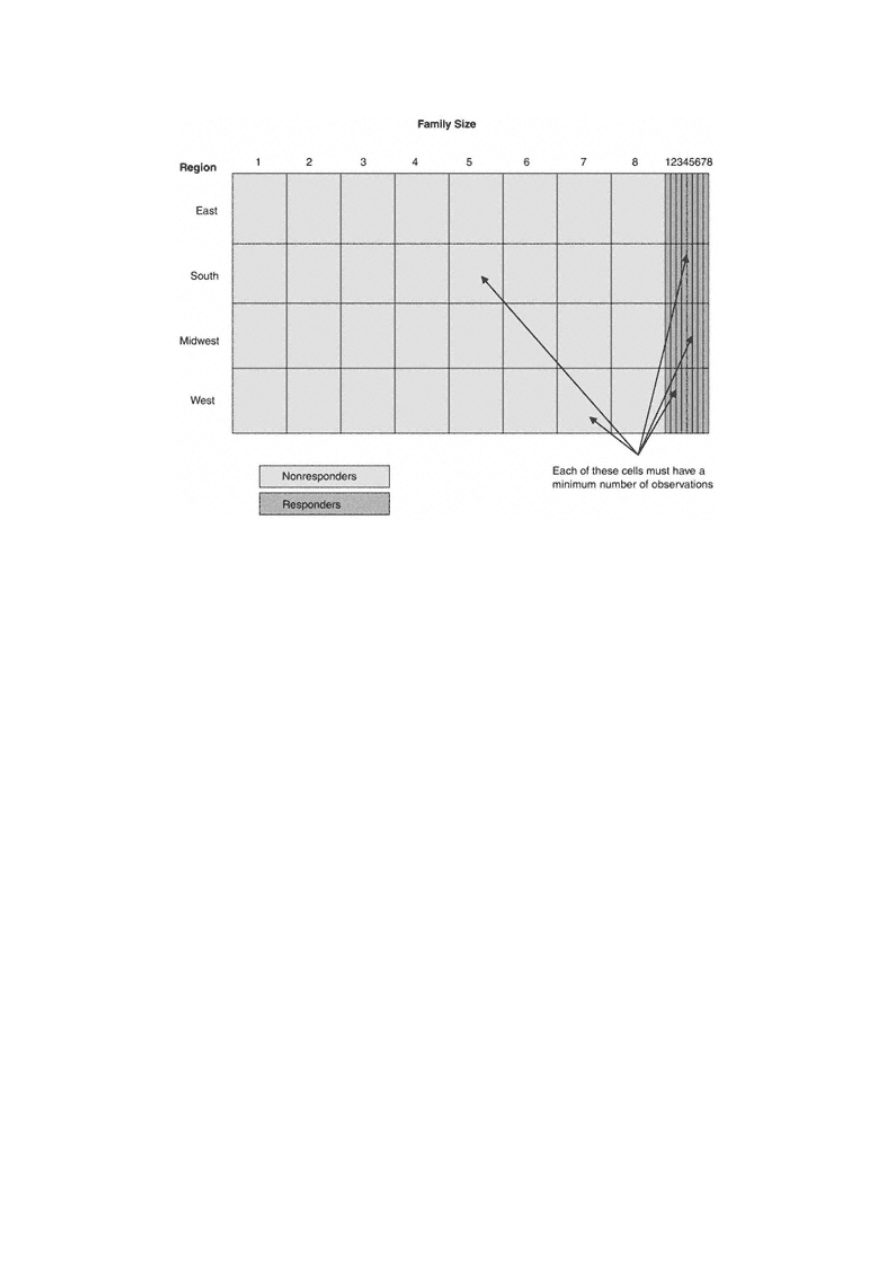
Page 45

Figure

2.2

Cross-section

variable

levels.

The optimal sample size also depends on the predictive power of the variables. It is more difficult to find predictive
power with a small sample. But if you do, you will generally have a robust model. Keep in mind that if you have much
smaller samples available for model development, it is still possible to build a model. It is just a little more difficult to
find the strong predictive relationships.

Sampling Methods

In most situations a simple random sample will serve your modeling needs. If you plan to develop a model to replace a
current model, it is important to capture the behavior of the prospects that your current model would not normally select.
This can be accomplished by soliciting a randomly selected group of the names outside of the normal selects, as shown
in Figure 2.3. The idea is to select an "nth" random sample. When constructing the modeling data set, use a weight equal
to "n" for the random sample to re-create the entire universe. Be prepared for this to be a hard sell to management. This
group of names does not perform as well as the group that the model selects. Consequently, or for this portion of the
population, the company will probably lose money. Therefore, it is necessary to convince management of the value in
this information.

Page 46

Figure

2.3

Sampling

for

full

representation.

Stratified sampling works well if you have a characteristic that you want to use as a predictor but the prevalence of that
characteristic is very low. Stratified sampling simply means that you sample different segments of the population at
different rates or "nths." For example, let's say you know that gender is a strong predictor for your product, but the list
you are using to create your sample for model development is made up mostly of males. At some future date you plan to
use the model to score a different list that is more evenly split on gender. When you select the names for your offer, pull
a 1/1,000 sample from the males and a 1/100 sample from the females. This will pull in 10 times as many females as
males.

To select different sample sizes within the population, you create separate random samples within each distinct group.
The following SAS code details the steps:

data male(where=(ranuni(5555)<.001))
female(where=(ranuni(5555)<.01));
set.libname.list;
if gender = 'M' then output male;
else output female;
run;

data libname.sample;
set male female;
if gender = 'M' then weight = 1000; else weight = 100;
run;

Page 47

You may want to use weights in the modeling process to maintain the correct proportions. In the last section of the code,
the data is joined together and weights are assigned to re-create the original sample proportions.

Developing Models from Modeled Data

Many analysts who are tasked with building a model have similar complaints. They are asked to build a model on data
that was collected from a campaign where a model was used for the original name selection. In other words, they do not
have a full representation of the universe of available names. Unfortunately, this is very often the case. When this
occurs, you have a couple of choices. If the available sample represents greater than 80% of the total universe of names,
you have a good chance of developing a model that will generalize to the entire universe. Depending on the strength of
the new model and its ability to rank order the names, you might want to sample the nonselected names when you
implement the model so you can perform additional validation.

If the available sample represents less than 80% of the total universe of names, you have two choices. You can mail a
random sample of the entire population and wait for the results to build the model. Most companies would not tolerate
this delay. Another choice is to include the names that were not solicited in the nontarget group. Because these names
were not selected by the previous model they would presumably have a lower return rate. The resulting model would not
be optimal, but it could provide improved targeting until a better model development sample is available.

Combining Data from Multiple Offers

Many campaigns consist of multiple offers to the same prospect or customer. For example, a bank mails a credit offer to
a list of 100,000 prospects. Two weeks later the bank mails the same offer to the "best" 50,000 prospects from the same
list. "Best" is defined by a score to rank the probability of response. And a third offer is mailed two weeks later to the
"best" 25,000. In this situation, constructing the model development sample is not straightforward. You can't just look at
the first mailing because a nonresponder in the first mailing might be a responder in a later mailing. If you combine all
three mailings, though, you can have multiple records for the same person and the possibility of different outcomes for
each.

One method for constructing the model development sample is to combine all three mailings. Then reduce the total mail
file to one unique record per person. And finally, append the response activity to each record from any of the three

Page 48

mailings. This will allow you to take advantage of all the response activity. The model should be very robust; however,
it will not accurately calculate probabilities. Therefore this model should be used only for ranking the names from most
responsive to least responsive.

Summary

We've seen that data for developing targeting models comes in many forms and from many sources. In the course of
business there are a myriad of ways to create and simulate model development data to target almost any goal. And
finally, constructing the development data set leaves room for using your creativity. The most important point to
remember is this: "Your model is only as good as your data!"

Now that we've planned the menu and gathered the ingredients, we are really ready to get cookin'. In part 2, we get into
the nitty gritty. Beginning in chapter 3, we develop a model using a case study that takes us through chapter 7. So get
your apron on and let's start cooking!

Page 49

PART TWO—
THE COOKING DEMONSTRATION

Page 50

Have you ever seen the commercials for a miracle food processor? It slices! It dices! It purees! It mixes, chops, and
blends! This is where we begin our cooking demonstration! We start with raw data. We slice and dice the data and fill in
where there are missing ingredients. We finally get the data ready for processing! Once the data ingredients are ready,
we start cooking, testing, and evaluating our creation. Then we prepare to serve the finished product!

We begin our case study in part 2. Over the next five chapters, I develop a net present value model for a life insurance
direct-mail campaign. Chapter 3 introduces the components of the model and discuss steps for preparing the data.
Chapter 4 describes how the variables are selected and transformed to create the best fit. Chapter 5 is where the fun
begins! We process the model and look at the initial results. Chapter 6 takes the model through some rigorous validation.
And, finally, chapter 7 details the implementation, back-end validation, and maintenance.

As we delve into the details that take us through our case study, I include portions of the SAS code necessary to
complete the task. As I explain the steps in the text, I refer to sections of the code that appear in boldface. These are the
key steps for each data step or procedure and can be modified to fit data for numerous objectives over a variety of
industries.

So don your aprons and let's start cooking!

Page 51

Chapter 3—
Preparing the Data for Modeling

Data preparation is one of the most important steps in the model development process. From the simplest analysis to the
most complex model, the quality of the data going in is key to the success of the project. The famous saying ''Garbage
in, garbage out" is quite fitting in this case. The ability of a model to produce robust results is as dependent on good data
as it is on effective techniques.

Gaining access to the data and understanding its characteristics are the first steps to ensuring a good model. I begin
chapter 3 with basic steps for reading in and combining data from multiple sources. Once the modeling data set is built, I
begin the extremely boring but critically important task of cleaning the data. This involves looking for and handling data
errors, outliers, and missing values. Once the data is accessed and cleaned, I create some routine variables through
summarization, ratios, and date math. On completion of these steps, I have a data set worthy of modeling.

Accessing the Data

Before I begin the modeling process, I need to understand how data is classified and the various ways in which data is
transported. Obtaining the data in a usable format is the first step in the data preparation process. Depending on the type
of model you are developing, you may have to extract the data yourself or request it from an outside source. If you are
developing a model using data on

Page 52

existing customers, you may be able to pull the desired records from a data warehouse. This data typically arrives in a
usable format such as an SAS data set. If you are developing a model on an outside list or a prospect file, however, you
may have some choices about the record format of the data.

If you are obtaining data for model development from an outside source or a separate internal source, request the data in
ASCII (American Standard for Computer Information Interchange). An ASCII file is also known as a flat file or text
file. The rows represent individual records or observations, and the columns or fields represent the characteristics or
variables related to the records. An ASCII file comes in two basic record length formats, fixed and variable. (The format
of the record should not be confused with the format of the data, which is discussed later.)

A fixed format is the easiest to read because it uses a fixed amount of space for each characteristic. Each row of data is
the same length. The disadvantage of the fixed format is that it uses space for blank fields. Therefore, if many of the
fields have missing values, it can be wasteful.

Figure 3.1 displays the first five records of a sample flat file in a fixed record format. The first nine spaces contain the
prospect ID. The next space contains a geographic indicator. In the fifth record, the value for the geographic indicator is
missing. Following the geographic indicator is the zip code. Notice that the zip code has nine digits. This is typically
read in two separate fields. The last three fields are each one digit representing age group, gender, and marital status.

Notice the spaces in the first, second, and fifth rows. They will be read as missing values. They serve as placeholders to
keep each field lined up with the proper field name. The following code reads in the fixed format data:

data libname.fixed;
infile 'C:\fixedfile.txt' missover recl=22;
input
pros_id 1 -9 /*unique prospect identifier*/
region $ 10 /*region of country*/
zip5 $ 11-15 /*five digit zipcode*/
zip4 $ 16-19 /*four digit zip extension*/

0 -- 5 -- 10 -- 15 -- 20 --

000000001S800143437B S
000000002N19380 CFD
000000003S008083522BMW
000000004W945912441EMD
000000005 696441001AFS

Figure

3.1

Fixed

format.

Page 53

age_grp $ 20 /*age group*/
gender $ 21 /*gender*/
marital $ 22 /*marital status*/
;
run;

The code states exactly where each record begins and ends. It also uses a "$" before the variable to designate whether
the format of the data is character or numeric. (Other data formats may be used for certain types of data. Contact your
data source for guidance in reading alternate data formats.)

A variable format has the same structure for each row. The difference is in the column values or fields. If a column
value is missing, no space is used for that field. A placeholder or delimiter is used to separate each value. Some
examples of delimiters are commas, slashes, and spaces.

Figure 3.2 displays the first five records of a sample flat file in a variable format with a comma delimiter. The data is
identical to the fixed format data; it is just separated using commas. There is one major advantage of this type of format.
If there are a lot of missing values, the data takes up less space.

Notice how the spaces for missing values have two commas in a row. That tells the program to hold a space for the next
variable in line. The "$" denotes a character variable. The following code reads in the variable format data:

data libname.variable;
infile 'C:\varfile.txt' delimiter=',';
input
pros_id /*unique prospect identifier*/
region $ /*region of country*/
zip5 $ /*five digit zipcode*/
zip4 $ /*four digit zip extension*/
age_grp $ /*age group*/
gender $ /*gender*/
marital $ /*marital status*/
;
run;

0 -- 5 -- 10 -- 15 -- 20 --
000000001,S,80014,3437,B,,S
000000002,N,19380,,C,F,D
000000003,S,00808,3522,B,M,W
000000004,W,94591,2441,E,M,D
000000005,,69644,1001,A,F,S

Figure

3.2

Variable

format.

Team-Fly

Page 54

It is also important to request all supporting documentation such as a file layout and data dictionary. The file layout will
tell you the variable names, the starting position of the data and length of field for each character, and the type of
variable. The data dictionary will provide the format and a detailed description of each variable. It is also recommended
to get a "data dump" or printout of the first 25–100 records. This is invaluable for seeing just what you are getting.

Classifying Data

There are two classes of data, qualitative and quantitative. Qualitative data use descriptive terms to differentiate values.
For example, gender is generally classified into "M" or male and "F" or female. Qualitative data can be used for
segmentation or classification. Quantitative data is characterized by numeric values. Gender could also be quantitative if
prior rules are established. For example, you could say that the values for gender are 1 and 2 where 1 = "M" or male and
2 = "F" or female. Quantitative data is used for developing predictive models. There are four types of quantitative data.

Nominal data is numeric data that represents categories or attributes. The numeric values for gender (1 & 2) would be
nominal data values. One important characteristic of nominal data is that it has no relative importance. For example,
even though male = 1 and female = 2, the relative value of being female is not twice the value or a higher value than that
of being male. For modeling purposes, a nominal variable with only two values would be coded with the values 0 and 1.
This will be discussed in more detail in chapter 4.

Ordinal data is numeric data that represents categories that have relative importance. They can be used to rank strength
or severity. For example, a list company assigns the values 1 through 5 to denote financial risk. The value 1,
characterized by no late payments, is considered low risk. The value 5, characterized by a bankruptcy, is considered high
risk. The values 2 through 4 are characterized by various previous delinquencies. A prospect with a risk ranking of 5 is
definitely riskier than a prospect with a ranking of 1. But he or she is not five times as risky. And the difference in their
ranks of 5 – 1 = 4 has no meaning.

Interval data is numeric data that has relative importance and has no zero point. Also, addition and subtraction are
meaningful operations. For example, many financial institutions use a risk score that has a much finer definition than the
values 1 through 5, as in our previous example. A typical range is from 300 to 800. It is therefore possible to compare
scores by measuring the difference.

Continuous data is the most common data used to develop predictive models. It can accommodate all basic arithmetic
operations, including addition,

Page 55

subtraction, multiplication, and division. Most business data such as sales, balances, and minutes, is continuous
data.

Reading Raw Data

Data formats are used to read each column or data field in its most useful form. The two most common formats are
character and numeric. If you do not have a sample of the data to view and you are not sure of the type of data, it is
advisable to read in the first 25–50 records with every field in character format. This takes very little time, allows you to
test your code, and lets you print the first few records to get a good look at the data.

To create the modeling data set for our insurance case study I begin with two separate files:

The original acquisition campaign offer file has 729,228 records. It contains a prospect identifier along with 43
demographic, credit, and segmentation characteristics. It is a flat file with a fixed record length. It was a direct mail offer
that was rolled out to the state of New York six months ago.

The performance file has 13,868 records and represents the responders to this campaign. It contains a prospect
identifier and an activation flag. The activation flag indicates that the prospect passed the risk screening and paid the
first premium. The file is a flat file with a fixed record length.

The input process begins with knowing the format of the data. The following code reads the entire campaign offer file
and prints the first 25 records. The first line sets up the library, acqmod. The second line creates an SAS data set,
acqmod.campaign. The infile statement identifies the flat file to read. The missover option tells the program to skip over
missing values. And the recl=109 defines the length of each line so the program knows when to go to a new record. The
"$" denotes a character or nonnumeric variable. The variable names are all held to seven characters to allow for numeric
extensions later in the processing:

libname acqmod 'c:\insur\acquisit\modeldata';

data acqmod.campaign;
infile 'F:\insur\acquisit\camp.txt' missover recl=109;
input
pros_id 1-9 /*unique prospect identifier*/
pop_den $ 13 /*population density code*/
trav_cd $ 14 /*travel indicator*/
bankcrd $ 15 /*presence of bankcard*/
deptcrd $ 16 /*presence of dept store card*/
fin_co $ 17 /*pres of finance co. loan*/
premcrd $ 18 /*pres of premium bankcard*/
upsccrd $ 19 /*pres of upscale bankcard*/
apt_ind $ 20 /*apartment indicator*/

Page 56

pob_ind $ 21 /*P.O.Box indicator*/
clustr1 $ 22 -23 /*statistical grouping*/
inc_est 24 -27 /*estimated income in dollars*/
inc_grp $ 28 /*income group*/
sgle_in $ 29 /*marital status = single*/
opd_bcd $ 30 -35 /*bankcard open date*/
occu_cd $ 36 /*occupation code*/
finl_id $ 37 /*finance loan identifier*/
gender $ 38 /*gender*/
ssn_ind $ 39 /*presence of SOC SEC Number*/
driv_in $ 40 /*driver indicator*/
mob_ind $ 41 /*mail order buyer indicator*/
mortin1 $ 42 /*presence of first mortgage*/
mortin2 $ 43 /*presence of second mortgage*/
autoin1 $ 44 /*presence of one auto loan*/
autoin2 $ 45 /*presence of two auto loans*/
infd_ag 46 -47 /*inferred age*/
age_ind $ 48 /*indicator - how age derived*/
dob_yr $ 49 -52 /*year of birth*/
homeq_r $ 53 /*home equity range*/
hom_equ $ 54 -61 /*home equity*/
childin $ 62 /*presence of child indicator*/
homevlr $ 63 /*home value range*/
clustr2 $ 64 /*statistical grouping*/
tot_acc 65 -67 /*total credit accounts*/
actopl6 68 -70 /*# accts open in last 6 mos*/
credlin 71 -77 /*total credit lines*/
tot_bal 78 -84 /*total credit card balances*/
inql6m 85 -87 /*# credit inq. last 6 months*/
age_fil 88 -90 /*age of file*/
totopac 91 -93 /*total open credit accounts*/
no30day 94 -96 /*number 30 day late ever*/
no90eve 97 -99 /*number 90 day late ever*/
nobkrpt 100 -102 /*number of bankruptcies*/
amtpdue 103 -109 /*total currently past due*/
;
run;

options obs=25;
proc print;
title 'XYZ Life Insurance Campaign Data - 25 Records';
run;

The next code reads the performance data and prints the first 25 records. It also creates a variable respond that has the
value of 1 for every record. Before I begin to read in the campaign data, I reset the obs=max option. This overwrites the
options obs=25 in the previous step.

options obs=max;

Page 57

data acqmod.response;
infile 'F:\insur\acquisit\perform.txt' missover recl=10;
input
pros_id 1-9 /*unique prospect identifier*/
activate $ 10 /*activation indicator*/
;
respond = 1;
run;

options obs=25;
proc print;
title 'Life Insurance Performance Data - 25 Records';
run;

At this point, I have both the prospect file and responder file read into SAS data sets. In the next section, I combine them
to make the modeling data set.

Creating the Modeling Data Set

In chapter 2, I described sources of data for model development. In many cases it is necessary to combine data from
several sources. As explained earlier, I have two data sets that need to be combined to create the final data set: the
original campaign data file and the performance data. The performance file contains only those prospects who responded
and a flag to indicate whether they activated. Both files contain a unique identifier, called a prospect ID (pros_id), for
each record that can be used to match the policyholders back to the original campaign data. To combine files in a data
step using SAS, it is necessary to sort the data by the field being used to combine the data. In our case study, I am using
prospect ID. Before I create the modeling data set, I should consider whether I want to reduce the size of the modeling
data set using sampling.

options obs=max;

proc sort data=acqmod.campaign;
by pros_id;
run;

proc sort data=acqmod.response;
by pros_id;
run;

data acqmod.both;
merge acqmod.campaign acqmod.response;
by pros_id;
run;
;

Page 58

TIP

In many cases, you are asked to merge files that do not have a unique identifier for
matching. In this situation, the most common method for merging is using name and
address. There are an unlimited number of ways to configure the name and address for
matching. The most cost-effective way to act on this is to use a proven software package.
They make use of years of experience and offer great flexibility.

Sampling

Computer power has improved dramatically over the last few years. It might be argued that sampling isn't necessary for
saving time and space, but it still makes good sense. It speeds up the process and generally produces the same results.

In target modeling, the target group is often a small percentage (< 10%) of the total population. In this situation, the best
approach is to keep the entire target group and extract a random sample from the nontarget group. A sample of 50,000 to
75,000 for the nontarget group is usually optimal. You can always use less. It just becomes more difficult to develop a
model with a high number of variables. If your results are significant, however, your model will be more robust.

In the case study, I have 13,868 responders and 715,360 nonresponders. My target group is actually a subset of the
responders. I keep all of the responders and take a 1/10th random sample from the nonresponders. The following code
creates the final data set. A frequency is run on the performance variables using weights for verification. The output
from the frequency is seen in Figure 3.3. This exercise allows you to validate that the weights have been applied
correctly. The final sample configuration is displayed in Table 3.1.

options obs=max;

data nonresp(where=(ranuni(5555)<.1));
set acqmod.both(where=(respond^=1));
run;

data acqmod.model;
set acqmod.both(where=(respond=1)) nonresps;
if respond = 1 then smp_wgt = 1;
else smp_wgt = 10;
respond = (respond = 1);
run;

proc freq;
weight smp_wgt;
table respond activate /missing;
run;

Page 59

Figure

3.3

Sample

frequences.

The sample frequencies show the number of records in the file and the sample. This is summarized in Table
3.1.

WARNING

It is important to match the responders to the file and determine who are the
nonresponders before you take the sample. Otherwise, you might not get all the data for
the responders.

Table 3.1

Modeling Sample Data Set

GROUP

CAMPAIGN

SAMPLE

WEIGHT

Actives

1,602

Responders/Nonactive

12,806

Nonresponders

715,360

71,536

Total

729,768

85,944

Page 60

Cleaning the Data

I now have the complete data set for modeling. The next step is to examine the data for errors, outliers, and missing
values. This is the most time-consuming, least exciting, and most important step in the data preparation process. Luckily
there are some effective techniques for managing this process.

First, I describe some techniques for cleaning and repairing data for continuous variables. Then I repeat the process for
categorical variables.

Continuous Variables

To perform data hygiene on continuous variables, PROC UNIVARIATE is a useful procedure. It provides a great deal
of information about the distribution of the variable including measures of central tendency, measures of spread, and the
skewness or the degree of imbalance of the data.

For example, the following code will produce the output for examining the variable estimated income
(inc_est).

proc univariate data=acqmod.model plot;
weight smp_wgt;
var inc_est;
run;

The results from PROC UNIVARIATE for estimated income (inc_est) are shown in Figure 3.4. The values are in
thousands of dollars.

There is a lot of information in this univariate analysis. I just look for a few key things. Notice the measures in bold. In
the moments section, the mean seems reasonable at $61.39224. But looking a little further I detect some data issues.
Notice that the highest value in the extreme values is 660. In Figure 3.5, the histogram and box plot provide a good
visual analysis of the overall distribution and the extreme value. I get another view of this one value. In the histogram,
the bulk of the observations are near the bottom of the graph with the single high value near the top. The box plot also
shows the limited range for the bulk of the data. The box area represents the central 50% of the data. The distance to the
extreme value is very apparent. This point may be considered an outlier.

Outliers and Data Errors

An outlier is a single or low-frequency occurrence of the value of a variable that is far from the mean as well as the
majority of the other values for that variable. Determining whether a value is an outlier or a data error is an art as well as
a science. Having an intimate knowledge of your data is your best strength.

Figure

3.4

Initial

univariate

analysis

estimated

income.

Figure

3.5

Histogram

and

box

plot

of estimated

income.

Page 62

Common sense and good logic will lead you to most of the problems. In our example, the one value that seems
questionable is the maximum value (660). It could have an extra zero. One way to see if it is a data error is to look at
some other values in the record. The variable estimated income group serves as a check for the value. The following
code prints the record:

proc print data=acqmod.model(where=(inc_est=660));
var inc_grp;
run;

The following output shows the estimated income group is ''K":

OBS INC_GRP
85206 K

Based on the information provided with the data, I know the range of incomes in group K to be between $65,000 and
$69,000. This leads us to believe that the value 660 should be 66. I can verify this by running a PROC MEANS for the
remaining records in group K.

proc means data=acqmod.model maxdec = 2;
where inc_grp = 'K' and inc_est ^= 660;
var inc_est;
run;

The following SAS output validates our suspicion. All the other prospects with estimated income group = K have
estimated income values between 65 and 69.

Analysis Variable : INC_EST (K)
N Mean Std Dev Minimum Maximum
--------------------------------------------
4948 66.98 1.41 65.00 69.00
--------------------------------------------

Here I replace the value 660 with 66. When substituting a new value for a missing value, it is always a good idea to
create a new variable name. This maintains the integrity of the original data.

data acqmod.model;
set acqmod.model;
if inc_est = 660 then inc_est2 = 66;
else inc_est2 = inc_est;
run;

In Figure 3.6, we see the change in the histogram and the box plot as a result of correcting the outlier. The distribution is
still centered near a lower range of values, but the skewness is greatly decreased.

Team-Fly

Figure

3.6

Histogram

and

box

plot

of estimated

income

with

corrections.

If you have hundreds of variables, you may not want to spend a lot of time on each variable with missing or incorrect values. Time
techniques for correction should be used sparingly. If you find an error and the fix is not obvious, you can treat it as a missing value.

Outliers are common in numeric data, especially when dealing with monetary variables. Another method for dealing with outliers is to develop a
capping rule. This can be accomplished easily using some features in PROC UNIVARIATE. The following code produces an output data set with the
standard deviation (incstd) and the 99th percentile value (inc99 ) for estimated income (inc_est).

proc univariate data=acqmod.model noprint;
weight smp_wgt;
var inc_est;
output out=incdata std=incstd pctlpts=99 pctlpre=inc;
run;

data acqmod.model;
set acqmod.model;
if (_n_ eq 1) then set incdata(keep= incstd inc99);
if incstd > 2*inc99 then inc_est2 =
min(inc_est,(4*inc99));
else inc_est2 = inc_est;
run;

Page 64

The code in bold is just one example of a rule for capping the values of a variable. It looks at the spread by seeing if the
standard deviation is greater than twice the value at the 99th percentile. If it is, it caps the value at four times the 99th
percentile. This still allows for generous spread without allowing in obvious outliers. This particular rule only works for
variables with positive values. Depending on your data, you can vary the rules to suit your goals.

Missing Values

As information is gathered and combined, missing values are present in almost every data set. Many software packages
ignore records with missing values, which makes them a nuisance. The fact that a value is missing, however, can be
predictive. It is important to capture that information.

Consider the direct mail company that had its customer file appended with data from an outside list. Almost a third of its
customers didn't match to the outside list. At first this was perceived as negative. But it turned out that these customers
were much more responsive to offers for additional products. After further analysis, it was discovered that these
customers were not on many outside lists. This made them more responsive because they were not receiving many direct
mail offers from other companies. Capturing the fact that they had missing values improved the targeting model.

In our case study, we saw in the univariate analysis that we have 84 missing values for income. The first step is to create
an indicator variable to capture the fact that the value is missing for certain records. The following code creates a
variable to capture the information:

data acqmod.model;
set acqmod.model;
if inc_est2 = . then inc_miss = 1;
else inc_miss = 0;
run;

The goal for replacing missing values is twofold: to fill the space with the most likely value and to maintain the overall
distribution of the variable.

Single Value Substitution

Single value substitution is the simplest method for replacing missing values. There are three common choices: mean,
median, and mode. The mean value is based on the statistical least-square -error calculation. This introduces the least
variance into the distribution. If the distribution is highly skewed, the median may be a better choice. The following
code substitutes the mean value for estimated income (inc_est2):

Page 65

data acqmod.model;
set acqmod.model;
if inc_est2 = . then inc_est3 = 61;
else inc_est3 = inc_est2;
run;

Class Mean Substitution

Class mean substitution uses the mean values within subgroups of other variables or combinations of variables. This
method maintains more of the original distribution. The first step is to select one or two variables that may be highly
correlated with income. Two values that would be highly correlated with income are home equity ( hom_equ) and
inferred age (infd_ag). The goal is to get the average estimated income for cross-sections of home equity ranges and age
ranges for observations where estimated income is not missing. Because both variables are continuous, a data step is
used to create the group variables, age_grp and homeq_r. PROC TABULATE is used to derive and display the values.

data acqmod.model;
set acqmod.model;
if 25 <= infd_ag <= 34 then age_grp = '25-34'; else
if 35 <= infd_ag <= 44 then age_grp = '35-44'; else
if 45 <= infd_ag <= 54 then age_grp = '45-54'; else
if 55 <= infd_ag <= 65 then age_grp = '55-65';
if 0 <= hom_equ<=100000 then homeq_r = '$0 -$100K'; else
if 100000<hom_equ<=200000 then homeq_r = '$100-$200K'; else
if 200000<hom_equ<=300000 then homeq_r = '$200-$300K'; else
if 300000<hom_equ<=400000 then homeq_r = '$300-$400K'; else
if 400000<hom_equ<=500000 then homeq_r = '$400-$500K'; else
if 500000<hom_equ<=600000 then homeq_r = '$500-$600K'; else
if 600000<hom_equ<=700000 then homeq_r = '$600-$700K'; else
if 700000<hom_equ then homeq_r = '$700K+';
run;

proc tabulate data=acqmod.model;
where inc_est2^=.;
weight smp_wgt;
class homeq_r age_grp;
var inc_est2;
table homeq_r ='Home Equity',age_grp='Age Group'*
inc_est2=' '*mean=' '*f=dollar6.
/rts=13;
run;

The output in Figure 3.7 shows a strong variation in average income among the different combinations of home equity
and age group. Using these values for missing value substitution will help to maintain the distribution of the data.

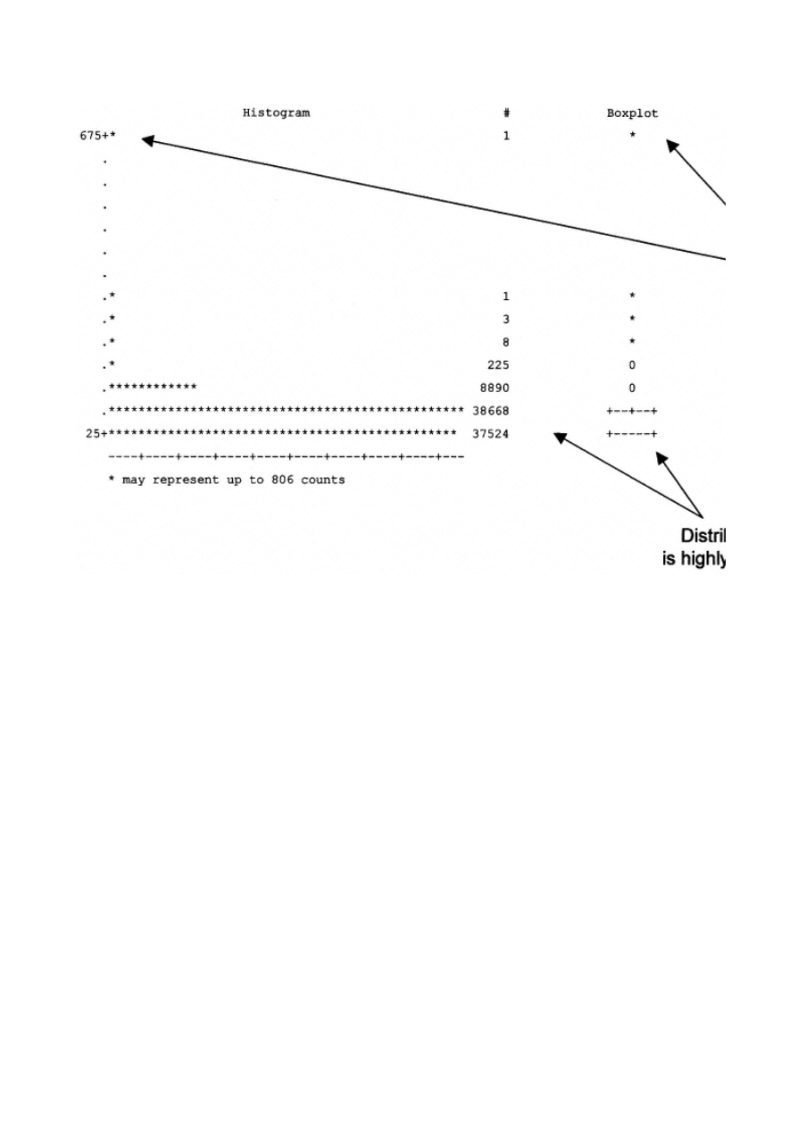
Figure

3.7

Values

for

class

mean

substitution.

The final step is to develop an algorithm that will create a new estimated income variable (inc_est3 ) that has no missing values.

data acqmod.model;
set acqmod.model;
if inc_est2 = . then do;
if 25 <= infd_ag <= 34 then do;
if 0 <= hom_equ<=100000 then inc_est3= 47; else
if 100000<hom_equ<=200000 then inc_est3= 70; else
if 200000<hom_equ<=300000 then inc_est3= 66; else
if 300000<hom_equ<=400000 then inc_est3= 70; else
if 400000<hom_equ<=500000 then inc_est3= 89; else
if 500000<hom_equ<=600000 then inc_est3= 98; else
if 600000<hom_equ<=700000 then inc_est3= 91; else
if 700000<hom_equ then inc_est3= 71;
end; else
if 35 <= infd_ag <= 44 then do;
if 0 <= hom_equ<=100000 then inc_est3= 55; else
if 100000<hom_equ<=200000 then inc_est3= 73; else
" " " "
" " " "
if 700000<hom_equ then inc_est3= 101;
end; else
if 45 <= infd_ag <= 54 then do;
if 0 <= hom_equ<=100000 then inc_est3= 57; else
if 100000<hom_equ<=200000 then inc_est3= 72; else
" " " "
" " " "

Page 67

if 700000<hom_equ then inc_est3= 110;
end; else
if 55 <= infd_ag <= 65 then do;
if 0 <= hom_equ<=100000 then inc_est3= 55; else
if 100000<hom_equ<=200000 then inc_est3= 68; else
" " " "
" " " "
if 700000<hom_equ then inc_est3= 107;
end;
end;
run;

Regression Substitution

Similar to class mean substitution, regression substitution uses the means within subgroups of other variables. The
advantage of regression is the ability to use continuous variables as well as look at many variables for a more precise
measurement. The resulting regression score is used to impute the replacement value.

In our case study, I derive values for estimated income (inc_est2) using the continuous form of age (infd_ag), the mean
for each category of home equity (hom_equ), total line of credit (credlin), and total credit balances (tot_bal). The
following code performs a regression analysis and creates an output data set (reg_out ) with the predictive coefficients.

proc reg data=acqmod.model outest=reg_out;
weight smp_wgt;
inc_reg: model inc_est2 = infd_ag hom_equ credlin tot_bal/ selection =
backward;
run;

Figure 3.8 shows a portion of the regression output. The parameter estimates are saved in the data set (reg_out ) and used
in PROC SCORE.

The following code is used to score the data to create inc_reg, the substitute value for income. A new data set is created
called acqmod.model2. This creates a backup data set.

proc score data=acqmod.model score=reg_out out=acqmod.model2
type=parms predict;
var infd_ag hom_equ credlin tot_bal;
run;

The following code creates inc_est3 using the regression value:

data acqmod.model2;
set acqmod.model2;
if inc_est2 = . then inc_est3 = inc_reg;
else inc_est3 = inc_est2;
run;

Page 68

Figure

3.8

Output

for

regression

substitution.

One of the benefits of regression substitution is its ability to sustain the overall distribution of the data. To measure the
effect on the spread of the data, I look at a PROC MEANS for the variable before (inc_est2) and after (inc_est3) the
substitution:

proc means data=acqmod.model2 n nmiss mean std min max;
weight smp_wgt;
var inc_est2 inc_est3;
run;

I see in Figure 3.9 that the distribution is almost identical for both variables. The 84 values from the regression (inc_reg)
that replaced the missing values in inc_est2 are a good match for the distribution.

These actions can be performed on all of the continuous variables. See Appendix A for univariate analysis of remaining
continuous variables. Now I must examine the quality of the categorical variables.

Page 69

Figure

3.9

Means

comparison

missing

replacement..

Categorical Variables

As I described earlier, categorical variables are very different from continuous variables. It is still important to look at
their distributions and handle any missing values.

Data Errors

A simple frequency is the best way to examine categorical variables for errors. Most categorical variables have a small
enough number of levels to view individually.

proc freq data=acqmod.model2;
weight smp_wgt;
table pop_den trav_cd bankcrd apt_ind clustr1 inc_grp sgle_in opd_bcd
occu_cd finl_id hh_ind gender ssn_ind driv_in mob_ind mortin1 mortin2
autoin1 autoin2 infd_ag age_ind dob_yr homeq_r childin homevlr clustr2
/ missing;
run;

In Figure 3.10, I see that population density (pop_den) has four values, A, B, C, and P. I requested the missing option in
our frequency, so I can see the number of missing values. The data dictionary states that the correct values for pop_den
are A, B, and C. I presume that the value P is an error. I have a couple of choices to remedy the situation. I can delete it
or replace it. For the purposes of this case study, I give it the value of the mode, which is C.

Missing Values

When modeling with nonnumeric (categorical) variables, the best way to handle missing values is to treat them as an
additional category. This will be covered in greater detail in chapter 4.

See Appendix B for simple frequencies of the remaining categorical variables.

Page 70

Figure

3.10

Frequency

population

density.

Summary

In this chapter I demonstrated the process of getting data from its raw form to useful pieces of information. The process
uses some techniques ranging from simple graphs to complex univariate outputs. But, in the end, it becomes obvious
that with the typically large sample sizes used in marketing, it is necessary to use these techniques effectively. Why?
Because the quality of the work from this point on is dependent on the accuracy and validity of the data.

Now that I have the ingredients, that is the data, I am ready to start preparing it for modeling. In chapter 4, I use some
interesting techniques to select the final candidate variables. I also find the form or forms of each variable that
maximizes the predictive power of the model.

Page 71

Chapter 4—
Selecting and Transforming the Variables

At this point in the process, the data has been carefully examined and refined for analysis. The next step is to define the
goal in technical terms. For our case study, the objective is to build a net present value (NPV) model for a direct mail
life insurance campaign. In this chapter, I will describe the components of NPV and detail the plan for developing the
model.

Once the goal has been defined, the next step is to find a group of candidate variables that show potential for having
strong predictive power. This is accomplished through variable reduction. To select the final candidate variables I use a
combination of segmentation, transformation, and interaction detection.

Defining the Objective Function

In chapter 1, I stressed the importance of having a clear objective. In this chapter, I assign a technical definition — called
the objective function— to the goal. Recall that the objective function is the technical definition of your business goal.

In our case study, the first goal is to predict net present value. I define the objective function as the value in today's
dollars of future profits for a life insurance product. The NPV for this particular product consists of four major
components: the probability of activation, the risk index, the product profitability, and the marketing expense. They are
each defined as follows:

Page 72

Probability of activation. A probability calculated by a model. The individual must respond, be approved by risk, and
pay his or her first premium.

Risk index. Indices in matrix of gender by marital status by age group based on actuarial analysis. This value can also
be calculated using a predictive model.

Product profitability. Present value of product-specific, three-year profit measure that is provided by the product
manager.

Marketing expense. Cost of package, mailing, and processing (approval, fulfillment).

The final model is a combination of these four components:

Net Present Value = P(Activation) × Risk Index × Product Profitability – Marketing Expense

For our case study, I have specific methods and values for these measures.

Probability of Activation

To calculate the probability of activation, I have two options: build one model that predicts activation or build two
models, one for response and one for activation, given response (model build on just responders to target actives). To
determine which method works better, I will develop the model both ways.

Method 1: One model. When using one model, the goal is to target active accounts, that is, those responders who paid
their first premium. To use the value ''activate" in the analysis, it must be in a numeric form, preferably 0 or 1. We know
from the frequency in chapter 3 that the values for the variable, activate, are as follows: activate = 1, respond but not
activated = 0, no response = (missing). To model activation from the original offer, I must give nonresponders the value
of 0. I create a new variable, active, and leave the original variable, activate, untouched.

data acqmod.model2;
set acqmod.model2;
if activate = . then active = 0;
else active = activate;
run;

We will now use the variable active as our dependent variable.

Method 2: Two models. When using two models, the goal is to build one model to target response and a second model
to target activation, given response. The probability of activation, P(A), is the product of the probability of response, P
(R), times the probability of activation, given response, P(A|R). For this method, I do not have to recode any of the
dependent vari-

Team-Fly

ables. The variables respond and activate are properly coded with the values of 0 and 1.

There are advantages and disadvantages to each method. Method 1 introduces less variance than the two-model approach in Method 2
simply because you are getting closer to your final goal with one model. The advantage of Method 2 is that it allows variables to enter the
model that may have the opposite relationship between response and activation. For example, if age is positively correlated with response
and negatively correlated with activation, it probably will not have any predictive power in Method 1. The opposite relationships will cancel
each other out. Method 2, on the other hand, might have the variable age with a positive sign for response and a negative sign for activation.
Another advantage to Method 2 is the ability to validate the models on the back end. In other words, if the model fails to perform as
expected, it might be caused by a change in the market that is affecting response. In that situation, you could rebuild the response portion of
the model. As we work through the case study, we track both methods to see which works better for our analysis.

Risk Index

The risk component of the NPV model is an index that was derived from a segmentation analysis on former customers. It represents an
adjustment to the final NPV based on age group, gender, and marital status. As you can see in Table 4.1, young married females have a
strong positive effect on profits. Conversely, single, elderly males have a negative effect on profits.

Product Profitability

For our case study, we received a value for the product profitability from the product manager of $811.30. This is based on the average
profits on the whole life policy, discounted in today's dollars. I will cover the methodology for discounting in chapter 12.

Table 4.1

Risk Matrix

MALE

FEMALE

AGE

MARRIED

SINGLE

DIVORCED

WIDOWED

MARRIED

SINGLE

DIVORCE

< 40

1.09

1.06

1.04

1.01

1.14

1.10

1.07

40–49

1.01

1.02

0.96

0.95

1.04

1.07

1.01

50–59

0.89

0.83

0.81

0.78

0.97

0.99

0.95

60+

0.75

0.65

0.72

0.70

0.94

0.89

0.84

Page 74

Marketing Expense

The marketing expense for this product is $.78. This is a combination of the cost of the mail piece, $.45, postage of $.23
per piece, and $.10 for processing.

Deriving Variables

Once the data is deemed correct and missing values have been handled, the next step is to look for opportunities to
derive new variables. This is a situation where knowledge of the data and the customer is critical. Combining variables
through summarization or division can improve predictive power. Additional analysis of dates and the use of "date
math" can assist in discovering new predictive variables.

Summarization

Summarization is an approach used to combine variables. This is done in certain cases where huge amounts of data are
generated. Some common methods include addition, subtraction, and averaging.

Consider the amount of data in an active credit card transaction file. Daily processing includes purchases, returns, fees,
and interchange income. Interchange income is the revenue that credit card banks collect from retailers for processing
payments through their system. To make use of this information, it is typically aggregated to daily, weekly, monthly, or
yearly totals and averages. For example, let's say you want to know the total monthly purchases for a group of
customers. And you want to know if that total is changing from month to month. First, you summarize the daily
purchases to get a monthly total. Then you subtract the months to get the difference.

The following code is not part of the case study, but it does represent an example of how to calculate the monthly totals,
average daily purchases, and amount of monthly change:

data ccbank.dailyact;
set ccbank.dailyact;

janpurch = sum(of pur0101 -pur0131); /* Summarize daily purchases */
febpurch = sum(of pur0201 -pur0208);
| | | | | |
decpurch = sum(of pur1201 -pur1231);
janavep = janpurch/31; /* Average daily purchases */
febavep = febpurch/28;

change1 = janpurch - febpurch; /* Calculate monthly change */

Page 75

change2 = febpurch - marpurch;
run;

Ratios

Ratios are another variable form that is very useful for certain types of prediction. Many values have additional meaning
when compared to some other factor. In this example, I have the variable credit line (credlin2 ). (Some variables now
have a "2" on the end after having missing values replaced.) It represents the total credit line for all credit accounts. A
total credit line is something people tend to build over time. To capture the value, I create a variable equal to the ratio of
credit line to age of file (age_fil2). The following code creates the variable crl_rat.

data acqmod.model2;
set acqmod.model2;

if age_fil2 > 0 then crl_rat=credlin2/age_fil2;
else crl_rat = 0;
run;

Dates

Dates are found in almost every data set. They can be very predictive as time measures or used in combination with
other dates or different types of variables. In order to use them it is necessary to get them into a format that supports
"date math." Date math is the ability to perform mathematical functions on dates. This includes addition, subtraction,
multiplication, and division. SAS has numerous formats to capture date values. Once you put a date into an SAS format,
it is stored as a whole number that represents the number of days since January 1, 1960. If you have two dates, you can
compare them easily using this information.

In our case study, I have a date variable called bankcard open date (opd_bcd ). It contains six characters. The first four
characters represent the year; the last two characters represent the month. The first step is to get the date into an SAS
format. The mdy format takes the values inside the parentheses and assigns them to month, day, and year. For months, I
use the substr command to pick the values. It begins in the fifth position and takes two characters in substr(opd_bcd,
5,2). Year is pulled the same way, beginning in the first position and taking four characters.

Next, I create the variable fix_dat. This represents December 31, 1999. In the calculation, I use (fix_dat – opd_bcd2)/30
to represent the approximate number of months from the first bankcard open date to the end of 1999. Using date

Page 76

math, I create a variable that represents the ratio of the current balance to the age in months of the oldest bankcard. I call
this variable bal_rat.

data acqmod.model2;
set acqmod.model2;
opd_bcd2 = mdy(substr(opd_bcd,5,2),'01',substr
(opd_bcd,1,4));
fix_dat = mdy('12','31','1999');

if opd_bcd ^= '000000' then
bal_rat = tot_bal2/((fix_dat - opd_bcd2)/30);
else bal_rat = 0;
run;

Variable Reduction

There are many opportunities to create variables through combinations and permutations of existing variables. This is
one reason why familiarity with the data and the industry is so valuable. Once you've extracted, formatted, and created
all eligible variables, it's time to narrow the field to a few strong contenders.

Continuous Variables

If you have fewer than 50 variables to start, you may not need to reduce the number of variables for final eligibility in
the model. As the amount of data being collected continues to grow, the need for variable reduction increases. Some
analysts, especially those using credit and transaction-level data, may be starting with 3,000+ eligible variables.
Performing an in-depth analysis on each variable is not an efficient use of time. Many of the variables are correlated
with each other. If you eliminate some that might have predictive power, usually some other ones will step in to do the
job.

In the classic text Applied Logistic Regression [Hosmer and Lemshow, Wiley 1990], the authors recommend performing
a univariate logistic regression on each variable. But with a large number of variables, this can be very time-consuming.
It is simpler to use a procedure in SAS called PROC LOGISTIC. This is the same procedure that is used to build the
final model, but it also works well as a variable reduction tool.

As an option in the model processing, choose selection=stepwise maxstep=1 and details . (In chapter 5, I will cover the
selection options in more detail.) This will run very quickly because you are running only one step in the modeling
process.

Page 77

Method 1:
One Model

title1 "XYZ Insurance - Data Reduction";
proc logistic data=acqmod.model2 descending;
weight smp_wgt;
model active = inc_est3 inc_miss infd_ag2 hom_equ2 tot_acc2 actopl62
tot_bal2 inql6m2 age_fil2 totopac2 credlin2 crl_rat bal_rat no30day2
nobkrpt amtpdue no90eve
/selection= stepwise maxstep=1 details ;
run;

Part of the output will contain the table shown in Figure 4.1. From this table we can see the univariate predictive power
of each continuous variable.

To select the final variables, look in the last column. A good rule of thumb is to keep all variables with a probability of
chi-square of less than .5000. In our set of variables, all but NO30DAY and CRL_RAT remains in the candidate variable
set. So I will eliminate those two variables from consideration.

Let's repeat this exercise for the models in Method 2. We want to keep all variables that are eligible for any of the
models.

Figure

4.1

Analysis

variables

not

the

model.

Page 78

Chi-Square Statistic

In simple terms, the chi -square statistic measures the difference between what you expect to happen and
what actually happens. The formula reads:

If the chi-square value is large, then the p-value associated with the chi-square is small. The p -value
represents the probability that the event occurred by chance. The chi -square statistic is the underlying test for
many modeling procedures including logistic regression and certain classification trees.

Method 2:
Two Models

title2 "Modeling Response";
proc logistic data=acqmod.model2 descending;
weight smp_wgt;
model respond = inc_est3 inc_miss infd_ag2 hom_equ2 tot_acc2 actopl62
tot_bal2 inql6m2 age_fil2 totopac2 credlin2 crl_rat bal_rat no30day2
nobkrpt amtpdue no90eve /selection= stepwise maxstep=1 details;
run;

Figure 4.2 shows the univariate or individual predictive power of each variable when modeling response. All variables
have predictive power with estimated income (inc_est3 ) being the strongest predictor.

For predicting response, every variable is shown to be significant at the univariate level. I will allow all the variables to
be candidates in the final model. If we were looking at hundreds of variables, one way to reduce the number is to select
the 50 variables with the highest chi -square score.

title2 "Modeling Activiate";
proc logistic data=acqmod.model2 descending;
weight smp_wgt;
model activate = inc_est3 inc_miss infd_ag2 hom_equ2 tot_acc2 actopl62
tot_bal2 inql6m2 age_fil2 totopac2 credlin2 crl_rat bal_rat no30day2
nobkrpt amtpdue no90eve /selection= stepwise maxstep=1 details;
run;

In Figure 4.3, the univariate logistic regression results for activation given response shows three variables that are not
significant at a level above Pr > .5000. These three variables will be dropped from consideration in the final model.

Page 79

Figure

4.2

Analysis

variables

not

the

model— respond.

Figure

4.3

Analysis

variables

not

the

model— activate|response.

Page 80

Categorical Variables

As mentioned in chapter 2, categorical variables are those variables that have discrete values. An easy way to determine
if they have predictive power is to perform a simple chi-square test using PROC FREQ. The missing option is included
to see if the missing status has predictive power.

Method 1:
One Model

proc freq data=acqmod.model2;
weight smp_wgt;
table active*(pop_den bankcrd)
/missing chisq ;
run;

The frequency distribution in Figure 4.4 provides a lot of information. We can see that there are enough observations in
each level of the variable for significance testing. A good rule of thumb is at least 25 observations in each cell. The chi-
square statistic (24.817) shows high significance. There is a probability of

.001 (significance level) that no significant

relationship exists between activation and population density. To enter the final model, I want a significance level less
than .5. This variable is a good candidate for the final model.

The column percent equates to the different activation rates for each level of population density (pop_den). The group
for which pop_den is missing has a .09% activation rate. This compares to group A (densely populated) with an
activation rate of .11%. Groups B and C are almost identical with activation rates of .07%. Later in the chapter, I will
discuss how these values are used for collapsing the variable.

In Figure 4.5 we see that the chi-square statistic for the relationship between activation and the presence of a bankcard is
0.352 with a significance level of 0.553. This means that there is no statistically significant difference in activation rate
between those prospects with bankcards and those without. The column percents are very close at 13% and 15%. This
variable is not a good candidate for the final model processing.

Method 2:
Two Models

To evaluate variables in the two-model approach, we have to examine each variable for response (model 1) and
activation given response (model 2). The following code tests the predictive power of population density (pop_den) and
presence of bankcard (bankcrd) in predicting response.

Page 81

Figure

4.4

Table

active

population

density.

proc freq data=acqmod.model2;
weight smp_wgt;
table respond*(pop_den bankcrd)
/missing chisq;
run;

Page 82

Figure

4.5

Table

active

bankcard.

In Figure 4.6, the chi-square statistic of 85.859 shows a highly significant relationship between response and population
density. The column percents also show great variation in response rate between the different levels of population
density. This variable is a very good candidate for the final model.

Team-Fly

Page 83

Figure

4.6

Table

respond

population

density.

In Figure 4.7, the chi-square statistic of .515 shows a marginally significant relationship between response and the
presence of a bankcard. The column percents also show very little variation in response rate between the different

Page 84

Figure

4.7

Table

respond

bankcard.ecting.

Page 85

levels of population density. This variable is not a good candidate for the final model. Because the significance level is
< .5, I will keep it for further analysis.

proc freq data=acqmod.model2;
where respond = 1;
weight smp_wgt;
table activate*(pop_den bankcrd)
/missing chisq;
run;

In Figure 4.8, the chi-square statistic of 9.640 shows a fairly significant relationship between activation given response
and population density. The column percents also show some variation in response rate between the different levels of
population density. This variable is a good candidate for the final model.

In Figure 4.9, the chi-square statistic of .174 shows a no statistically significant relationship between activation given
response and presence of a bankcard. The column percents also show very little variation in activation rate between the
different levels of population density (7.27 versus 7.68). With a significance level of .676, this variable is not a good
candidate for the final model.

Developing Linear Predictors

As described in chapter 1, logistic regression is a powerful and robust statistical technique for predicting the probability
of an event occurring. By robust, I mean that the model will perform well and hold up over time. Because the predictors
are linear in the log of the odds (as defined in chapter 1), the trick is to get the predictors as linear as possible. There are
several ways to accomplish this. In our case study, I will demonstrate some techniques that are rigorous and thorough.
As a result, the predictors will be robust and have strong predictive power.

In our case study, we have a group of 20 variables that will be analyzed for final presentation in the model. Some are
continuous, and some are categorical. Logistic regression sees all predictive variables as continuous. So for the
noncontinuous variables, I will use indicator variables to trick the model into thinking they are continuous.

Continuous Variables

A continuous variable with no missing values can be used ''as is" as a predictor in a logistic model. To get the best model
fit and predictive power, however, it is often useful to transform and/or segment the continuous variable to create a more
linear relationship. One way to determine the best transformation or seg-

Page 86

Figure

4.8

Table

activate

population

density.

mentation of a continuous variable is to create several variations and use a forward logistic regression to select the best
fit. The first step is to break the continuous variable into segments.

Page 87

Figure

4.9

Table

activate

bankcard.

Page 88

Segmentation

Some analysts and modelers put all continuous variables into segments and treat them as categorical variables. This may
work well to pick up nonlinear trends. The biggest drawback is that it loses the benefit of the relationship between the
points in the curve that can be very robust over the long term. Another approach is to create segments for obviously
discrete groups. Then test these segments against transformed continuous values and select the winners. Just how the
winners are selected will be discussed later in the chapter. First I must create the segments for the continuous variables.

In our case study, I have the variable estimated income (inc_est3). To determine the best transformation and/or
segmentation, I first segment the variable into 10 groups. Then I will look at a frequency of est_inc3 crossed by the
dependent variable to determine the best segmentation.

An easy way to divide into 10 groups with roughly the same number of observations in each group is to use PROC
UNIVARIATE. Create an output data set containing values for the desired variable (inc_est3 ) at each tenth of the
population. Use a NOPRINT option to suppress the output. The following code creates the values, appends them to the
original data set, and produces the frequency table.

proc univariate data=acqmod.model2 noprint;
weight smp_wgt;
var inc_est3;
output out=incdata pctlpts= 10 20 30 40 50 60 70 80 90 100
pctlpre=inc;
run;

data acqmod.model2;
set acqmod.model2;
if (_n_ eq 1) then set incdata;
retain inc10 inc20 inc30 inc40 inc50 inc60 inc70 inc80 inc90 inc100;
run;

data acqmod.model2;
set acqmod.model2;
if inc_est3 < inc10 then incgrp10 = 1; else
if inc_est3 < inc20 then incgrp10 = 2; else
if inc_est3 < inc30 then incgrp10 = 3; else
if inc_est3 < inc40 then incgrp10 = 4; else
if inc_est3 < inc50 then incgrp10 = 5; else
if inc_est3 < inc60 then incgrp10 = 6; else
if inc_est3 < inc70 then incgrp10 = 7; else
if inc_est3 < inc80 then incgrp10 = 8; else
if inc_est3 < inc90 then incgrp10 = 9; else
incgrp10 = 10;
run;

Page 89

proc freq data=acqmod.model2;
weight smp_wgt;
table (activate respond active)*incgrp10;
run;

From the output, we can determine linearity and segmentation opportunities. First we look at inc_est3 (in 10 groups)
crossed by active (one model).

Method 1:
One Model

In Figure 4.10 the column percent shows the active rate for each segment. The first four segments have a consistent
active rate of around .20%. Beginning with segment 5, the rate drops steadily until it reaches segment 7 where it levels
off at around .10%. To capture this effect with segments, I will create a variable that splits the values between 4 and 5.
To create the variable I use the following code:

data acqmod.model2;
set acqmod.model2;
if incgrp10 <= 4 then inc_low = 1; else inc_low = 0;
run;

At this point we have three variables that are forms of estimated income: inc_miss, inc_est3, and inc_low. Next, I will
repeat the exercise for the two-model approach.

Method 2:
Two Models

In Figure 4.11 the column percents for response follow a similar trend. The response rate decreases steadily down with a
slight bump at segment 4. Because the trend downward is so consistent, I will not create a segmented variable

In Figure 4.12 we see that the trend for activation given response seems to mimic the trend for activation alone. The
variable inc_low, which splits the values between 4 and 5, will work well for this model.

Transformations

Years ago, when computers were very slow, finding the best transforms for continuous variables was a laborious
process. Today, the computer power allows us to test everything. The following methodology is limited only by your
imagination.

In our case study, I am working with various forms of estimated income (inc_est3). I have created three forms for each
model: inc_miss, inc_est3, and inc_low. These represent the original form after data clean-up (inc_est3) and two
segmented forms. Now I will test transformations to see if I can make

Page 90

Figure

4.10

Active

income

group.

Page 91

Figure

4.11

Response

income

group.

Page 92

Figure

4.12

Activation

income

group.

Team-Fly

Page 93

inc_est3 more linear. The first exercise is to create a series of transformed variables. The following code creates new
variables that are continuous functions of income:

data acqmod.model2;
set acqmod.model2;
inc_sq = inc_est3**2; /*squared*/
inc_cu = inc_est3**3; /*cubed*/
inc_sqrt = sqrt(inc_est3); /*square root*/
inc_curt = inc_est3**.3333; /*cube root*/
inc_log = log(max(.0001,inc_est3)); /*log*/
inc_exp = exp(max(.0001,inc_est3)); /*exponent*/

inc_tan = tan(inc_est3); /*tangent*/
inc_sin = sin(inc_est3); /*sine*/
inc_cos = cos(inc_est3); /*cosine*/

inc_inv = 1/max(.0001,inc_est3); /*inverse*/
inc_sqi = 1/max(.0001,inc_est3**2); /*squared inverse*/
inc_cui = 1/max(.0001,inc_est3**3); /*cubed inverse*/
inc_sqri = 1/max(.0001,sqrt(inc_est3)); /*square root inv*/
inc_curi = 1/max(.0001,inc_est3**.3333); /*cube root inverse*/

inc_logi = 1/max(.0001,log(max(.0001,inc_est3))); /*log inverse*/
inc_expi = 1/max(.0001,exp(max(.0001,inc_est3))); /*exponent inv*/

inc_tani = 1/max(.0001,tan(inc_est3)); /*tangent inverse*/
inc_sini = 1/max(.0001,sin(inc_est3)); /*sine inverse*/
inc_cosi = 1/max(.0001,cos(inc_est3)); /*cosine inverse*/
run;

Now I have 22 forms of the variable estimated income. I have 20 continuous forms and 2 categorical forms. I will use
logistic regression to find the best form or forms of the variable for the final model.

Method 1:
One Model

The following code runs a logistic regression on every eligible form of the variable estimated income. I use the maxstep
= 2 option to get the two best-fitting forms (working together) of estimated income.

proc logistic data=acqmod.model2 descending;
weight smp_wgt;
model active = inc_est3 inc_miss inc_low
inc_sq inc_cu inc_sqrt inc_curt inc_log inc_exp
inc_tan inc_sin inc_cos inc_inv inc_sqi inc_cui inc_sqri inc_curi
inc_logi inc_expi inc_tani inc_sini inc_cosi
/selection = stepwise maxstep = 2 details;

Page 94

The result of the stepwise logistic shows that the binary variable, inc_low, has the strongest predictive power. The only
other form of estimated income that works with inc_low to predict active is the transformation (inc_sqrt). I will
introduce these two variables into the final model for Method 1.

Summary of Stepwise Procedure

Variable Number Score Wald Pr >
Step Entered In Chi -Square Chi-Square Chi-Square
1 INC_LOW 1 96.0055 . 0.0001
2 INC_SQRT 2 8.1273 . 0.0044

Method 2:
Two Models

The following code repeats the process of finding the best forms of income. But this time I am predicting response.

proc logistic data=acqmod.model2 descending;
weight smp_wgt;
model respond = inc_est3 inc_miss inc_low
inc_sq inc_cu inc_sqrt inc_curt inc_log inc_exp
inc_tan inc_sin inc_cos inc_inv inc_sqi inc_cui inc_sqri inc_curi
inc_logi inc_expi inc_tani inc_sini inc_cosi
/ selection = stepwise maxstep = 2 details;

run;

When predicting response (respond), the result of the stepwise logistic shows that the inverse of estimated income,
inc_inv, has the strongest predictive power. Notice the extremely high chi-square value of 722.3. This variable does a
very good job of fitting the data. The next strongest predictor, the inverse of the square root (inc_sqri), is also predictive.
I will introduce both forms into the final model.

Summary of Forward Procedure

Variable Number Score Wald Pr >
Step Entered In Chi -Square Chi-Square Chi-Square

1 INC_INV 1 722.3 . 0.0001
2 INC_SQRI 2 10.9754 . 0.0009

And finally, the following code determines the best fit of estimated income for predicting actives, given that the prospect
responded. (Recall that activate is missing for nonresponders, so they will be eliminated from processing automatically.)

proc logistic data=acqmod.model2 descending;
weight smp_wgt;

Page 95

model activate = inc_est3 inc_miss inc_low
inc_sq inc_cu inc_sqrt inc_curt inc_log inc_exp
inc_tan inc_sin inc_cos inc_inv inc_sqi inc_cui inc_sqri inc_curi
inc_logi inc_expi inc_tani inc_sini inc_cosi
/ selection = stepwise maxstep = 2 details;

run;

When predicting activation given response (activation|respond), the only variable with predictive power is inc_low. I
will introduce that form into the final model.

Summary of Stepwise Procedure

Variable Number Score Wald Pr >
Step Entered In Chi -Square Chi-Square Chi-Square

1 INC_LOW 1 10.4630 . 0.0012

At this point, we have all the forms of estimated income for introduction into the final model. I will repeat this process
for all continuous variables that were deemed eligible for final consideration.

Categorical Variables

Many categorical variables are powerful predictors. They, however, are often in a form that is not useful for regression
modeling. Because logistic regression sees all predictors as continuous, I must redesign the variables to suit this form.
The best technique is to create indicator variables. Indicator variables are variables that have a value of 1 if a condition
is true and 0 otherwise.

Method 1:
One Model

Earlier in the chapter, I tested the predictive power of pop_den. The frequency table shows the activation rate by class of
pop_den.

In Figure 4.13, we see that the values B and C have identical activation rates of .13%. I will collapse them into the same
group and create indicator variables to define membership in each class or group of classes.

data acqmod.model2;
set acqmod.model2;
if pop_den = 'A' then popdnsA = 1; else popdensA = 0;
if pop_den in ('B','C') then popdnsBC = 1; else popdnsBC = 0;
run;

Notice that I didn't define the class of pop_den that contains the missing values. This group's activation rate is
significantly different from A and ''B & C."

Page 96

Figure

4.13

Active

population

density.

But I don't have to create a separate variable to define it because it will be the default value when both popdnsA and
popdnsBC are equal to 0. When creating indicator variables, you will always need one less variable than the number of
categories.

Method 2:
Two Models

I will go through the same exercise for predicting response and activation given response.

In Figure 4.14, we see that the difference in response rate for these groups seems to be most dramatic between class A
versus the rest. Our variable popdnsA will work for this model.

Figure 4.15 shows that when modeling activation given response, we have little variation between the classes. The
biggest difference is between "B & C" versus "A and Missing." The variable popdnsBC will work for this model.

At this point, we have all the forms of population density for introduction into the final model. I will repeat this process
for all categorical variables that were deemed eligible for final consideration.

Page 97

Figure

4.14

Response

population

density.

Figure

4.15

Activation

population

density.

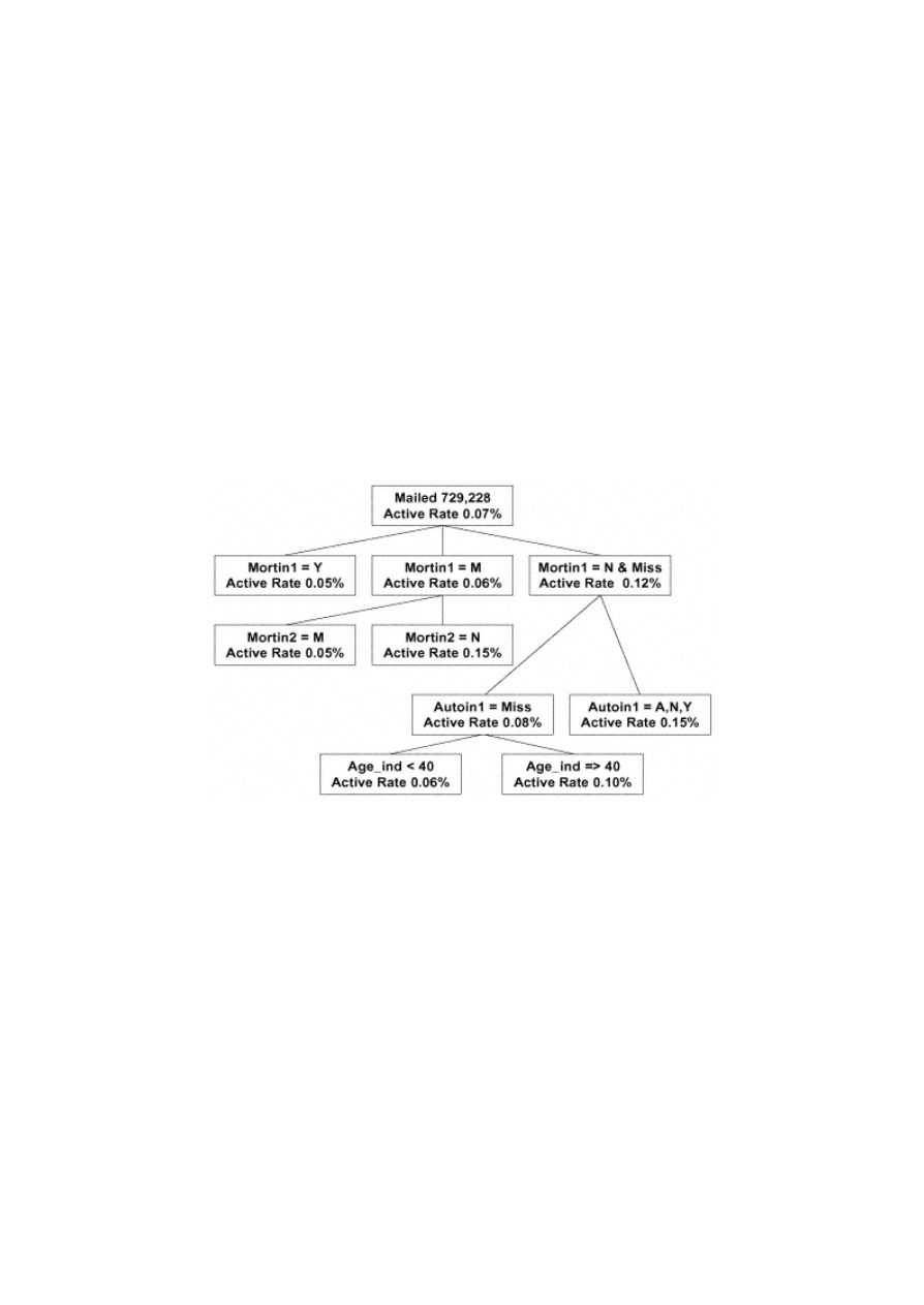
Page 98

Interactions Detection

An interaction between variables is said to be present if the relationship of one predictor varies for different levels of
another predictor. One way to find interactions between variables is to create combinations and test them for
significance. If you are starting out with hundreds of variables, this may not be a good use of time. In addition, if you
have even as many as 50 variables with univariate predictive power, you may not add much benefit by finding
interactions.

Many of the data mining software packages have a module for building classification trees. They offer a quick way to
discover interactions. In Figure 4.16, a simple tree shows interactions between mortin1, mortin2, autoin1, and age_ind .

The following code creates three variables from the information in the classification tree. Because these branches of the
tree show strong predictive power, these three indicator variables are used in the final model processing.

data acqmod.model2;
set acqmod.model2;
if mortin1 = 'M' and mortin2 = 'N' then mortal1 = 1;
else mortal1 = 0;
if mortin1 in ('N', ' ') and autoind1 = ' ' and infd_ag => 40)
then mortal2 = 1; else mortal2 = 0;

Figure

4.16

Interaction

detection

using

classification

trees.

Page 99

if mortin1 in ('N', ' ')
and autoin1 ^= ' ' then mortal3 = 1;
else mortal3 = 0;
run;

Summary

The emphasis of this chapter was on reducing the number of eligible variables. I did a lot of work ahead of time so that I
could have a clear goal and clean, accurate data. I started out with the development of some new variables that provide
added predictive power. In preparation for the final model processing, I used some simple techniques to reduce the
number of variables. These techniques eliminated variables that were marginal and unpredictive. They are especially
useful when you start out with hundreds of variables.

Next, through the use of some clever coding, I molded the remaining variables into strong predictors. And every step of
the way, I worked through the one-model and two-model approaches. We are now ready to take our final candidate
variables and create the winning model. In chapter 5, I perform the final model processing and initial validation.

Page 101

Chapter 5—
Processing and Evaluating the Model

Have you ever watched a cooking show? It always looks so easy, doesn't it? The chef has all the ingredients prepared
and stored in various containers on the countertop. By this time the hard work is done! All the chef has to do is
determine the best method for blending and preparing the ingredients to create the final product. We've also reached that
stage. Now we're going to have some fun! The hard work in the model development process is done. Now it's time to
begin baking and enjoy the fruits of our labor.

There are many options of methodologies for model processing. In chapter 1, I discussed several traditional and some
cutting-edge techniques. As we have seen in the previous chapters, there is much more to model development than just
the model processing. And within the model processing itself, there are many choices.

In the case study, I have been preparing to build a logistic model. In this chapter, I begin by splitting the data into the
model development and model validation data sets. Beginning with the one -model approach, I use several variable
selection techniques to find the best variables for predicting our target group. I then repeat the same steps with the two-
model approach. Finally, I create a decile analysis to evaluate and compare the models.

Page 102

Processing the Model

As I stated in chapter 3, I am using logistic regression as my modeling technique. While many other techniques are
available, I prefer logistic regression because (1) when done correctly it is very powerful, (2) it is straightforward, and
(3) it has a lower risk of over-fitting the data. Logistic regression is an excellent technique for finding a linear path
through the data that minimizes the error. All of the variable preparation work I have done up to this point has been to fit
a function of our dependent variable, active, with a linear combination of the predictors.

As described in chapter 1, logistic regression uses continuous values to predict a categorical outcome. In our case study,
I am using two methods to target active accounts. Recall that active has a value of 1 if the prospect responded, was
approved, and paid the first premium. Otherwise, active has a value of 0. Method 1 uses one model to predict the
probability of a prospect responding, being approved, and paying the first premium, thus making the prospect an
"active." Method 2 uses two models: one to predict the probability of responding; and the second uses only responders to
predict the probability of being approved and activating the account by paying the first premium. The overall probability
of becoming active is derived by combining the two model scores.

Following the variable reduction and creation processes in chapter 4, I have roughly 70 variables for evaluation in the
final model. Some of the variables were created for the model in Method 1 and others for the two models in Method 2.
Because there was a large overlap in variables between the models in Method 1 and Method 2, I will use the entire list
for all models. The processing might take slightly longer, but it saves time in writing and tracking code.

The sidebar on page 104 describes several selection methods that are available in SAS's PROC LOGISTIC. In our final
processing stage, I take advantage of three of those methods, Stepwise, Backward , and Score. By using several methods,
I can take advantage of some variable reduction techniques while creating the best fitting model. The steps are as
follows:

Why Use Logistic Regression?

Every year a new technique is developed and/or automated to improve the targeting model development
process. Each new technique promises to improve the lift and save you money. In my experience, if you take
the time to carefully prepare and transform the variables, the resulting model will be equally powerful and
will outlast the competition.

Page 103

Stepwise. The first step will be to run a stepwise regression with an artificially high level of significance. This will
further reduce the number of candidate variables by selecting the variables in order of predictive power. I will use a
significance level of .30.

Backward. Next, I will run a backward regression with the same artificially high level of significance. Recall that this
method fits all the variables into a model and then removes variables with low predictive power. The benefit of this
method is that it might keep a variable that has low individual predictive power but in combination with other variables
has high predictive power. It is possible to get an entirely different set of variables from this method than with the
stepwise method.

Score. This step evaluates models for all possible subsets of variables. I will request the two best models for each
number of variables by using the BEST=2 option. Once I select the final variables, I will run a logistic regression
without any selection options to derive the final coefficients and create an output data set.

I am now ready to process my candidate variables in the final model for both Method 1 (one-step model) and Method 2
(two-step model). I can see from my candidate list that I have many variables that were created from base variables. For
example, for Method 1 I have four different forms of infd_age: age_cui, age_cos, age_sqi, and age_low. You might ask,
"What about multicollinearity?" To some degree, my selection criteria will not select (forward and stepwise) and
eliminate (backward) variables that are explaining the same variation in the data. But it is possible for two or more forms
of the same variable to enter the model. Or other variables that are correlated with each other might end up in the model
together. The truth is, multicollinearity is not a problem for us. Large data sets and the goal of prediction make it a
nonissue, as Kent Leahy explains in the sidebar on page 106.

Splitting the Data

One of the cardinal rules of model development is, "Always validate your model on data that was not used in model
development." This rule allows you to test the robustness of the model. In other words, you would expect the model to
do well on the data used to develop it. If the model performs well on a similar data set, then you know you haven't
modeled the variation that is unique to your development data set.

This brings us to the final step before the model processing — splitting the file into the modeling and validation data sets.

Team-Fly

Page 104

TIP

If you are dealing with sparse data in your target group, splitting the data can leave you
with too few in the target group for modeling. One remedy is split the nontarget group
as usual. Then use the entire target group for both the modeling and development data
sets. Extra validation measures, described in chapter 6, are advisable to avoid over-
fitting.

Rather than actually creating separate data sets, I assign a weight that has a value equal to "missing." This technique
maintains the entire data set through the model while using only the "nonmissing" data for model development.

Selection Methods

SAS's PROC LOGISTIC provides several options for the selection method that designate the order in which
the variables are entered into or removed from the model.

Forward. This method begins by calculating and examining the univariate chi-square or individual
predictive power of each variable. It looks for the predictive variable that has the most variation or greatest
differences between its levels when compared to the different levels of the target variable. Once it has
selected the most predictive variable from the candidate variable list, it recalculates the univariate chi-square
for each remaining candidate variable using a conditional probability. In other words, it now considers the
individual incremental predictive power of the remaining candidate variables, given that the first variable has
been selected and is explaining some of the variation in the data. If two variables are highly correlated and
one enters the model, the chi-square or individual incremental predictive power of the other variable (not in
the model) will drop in relation to the degree of the correlation.

Next, it selects the second most predictive variable and repeats the process of calculating the univariate chi-
square or the individual incremental predictive power of the remaining variables not in the model. It also
recalculates the chi-square of the two variables now in the model. But this time it calculates the multivariate
chi-square or predictive power of each variable, given that the other variable is now explaining some of the
variation in the data.

Again, it selects the next most predictive variable, repeats the process of calculating the univariate chi-square
power of the remaining variables not in the model, and recalculates the multivariate chi-square of the three
variables now in the model. The process repeats until there are no significant variables in the remaining
candidate variables not in the model.

Page 105

The actual split can be 50/50, 60/40, 70/30, etc. I typically use 50/50. The following code is used to create a weight
value (splitwgt). I also create a variable, records, with the value of 1 for each prospect. This is used in the final
validation tables:

data acqmod.model2;
set acqmod.model2;
if ranuni(5555) < .5 then splitwgt = smp_wgt;
else splitwgt = .;
records = 1;
run;

Stepwise. This method is very similar to forward selection. Each time a new variable enters the model, the
univariate chi-square of the remaining variables not in the model is recalculated. Also, the multivariate chi-
square or incremental predictive power of each predictive variable in the model is recalculated. The main
difference is that if any variable, newly entered or already in the model, becomes insignificant after it or
another variable enters, it will be removed.

This method offers some additional power over selection in finding the best set of predictors. Its main
disadvantage is slower processing time because each step considers every variable for entry or removal.

Backward. This method begins with all the variables in the model. Each variable begins the process with a
multivariate chi-square or a measure of predictive power when considered in conjunction with all other
variables. It then removes any variable whose predictive power is insignificant, beginning with the most
insignificant variable. After each variable is removed, the multivariate chi-square for all variables still in the
model is recalculated with one less variable. This continues until all remaining variables have multivariate
significance.

This method has one distinct benefit over forward and stepwise. It allows variables of lower significance to
be considered in combination that might never enter the model under the forward and stepwise methods.
Therefore, the resulting model may depend on more equal contributions of many variables instead of the
dominance of one or two very powerful variables.

Score. This method constructs models using all possible subsets of variables within the list of candidate
variables using the highest likelihood score (chi-square) statistic. It does not derive the model coefficients. It
simply lists the best variables for each model along with the overall chi-square.

Page 106

Multicollinearity: When the Solution Is the Problem

Kent Leahy, discusses the benefits of multicollinearity in data analysis.

As every student of Statistics 101 knows, highly correlated predictors can cause problems in a regression or
regression-like model (e.g., logit). These problems are principally ones of reliability and interpretability of
the model coefficient estimates. A common solution, therefore, has been to delete one or more of the
offending collinear model variables or to use factor or principal components analysis to reduce the amount of
redundant variation present in the data.

Multicollinearity (MC), however, is not always harmful, and deleting a variable or variables under such
circumstances can be the real problem. Unfortunately, this is not well understood by many in the industry,
even among those with substantial statistical backgrounds.

Before discussing MC, it should be acknowledged that without any correlation between predictors, multiple
regression (MR) analysis would merely be a more convenient method of processing a series of bivariate
regressions. Relationships between variables then actually give life to MR, and indeed to all multivariate
statistical techniques.

If the correlation between two predictors (or a linear combination of predictors) is inordinately high,
however, then conditions can arise that are deemed problematic. A distinction is thus routinely made
between correlated predictors and MC. Although no universally acceptable definition of MC has been
established, correlations of .70 and above are frequently mentioned as benchmarks.

The most egregious aspect of MC is that it increases the standard error of the sampling distribution of the
coefficients of highly collinear variables. This manifests itself in parameter estimates that may vary
substantially from sample -to -sample. For example, if two samples are obtained from a given population, and
the same partial regression coefficient is estimated from each, then it is considerably more likely that they
will differ in the presence of high collinearity. And the higher the intercorrelation, the greater the likelihood
of sample-to-sample divergence.

MC, however, does not violate any of the assumptions of ordinary least-squares (OLS) regression, and thus
the OLS parameter estimator under such circumstances is still BLUE (Best Linear Unbiased Estimator). MC
can, however, cause a substantial decrease in ''statistical power," because the amount of variation held in
common between two variables and the dependent variable can leave little remaining data to reliably
estimate the separate effects of each. MC is thus a lack of data condition necessitating a larger sample size to
achieve the

Page 107

same level of statistical significance. The analogy between an inadequate sample and MC is cogently and
clearly articulated by Achen [1982]:

"Beginning students of methodology occasionally worry that their independent variables are correlated with the
so -called multicollinearity problem. But multi-collinearity violates no regression assumptions. Unbiased,
consistent estimates will occur, and the standard errors will be correctly estimated. The only effect of
multicollinearity is to make it harder to get coefficient estimates with small standard errors. But having a small
number of observations also has that effect. Thus, "What should I do about multicollinearity?" is a question
like "What should I do if I don't have many observations?"

If the coefficient estimates of highly related predictors are statistically significant, however, then the
parameter estimates are every bit as reliable as any other predictor. As it turns out, even if they are not
significant, prediction is still unlikely to be affected, the reason being that although the estimates of the
separate effects of collinear variables have large variances, the sum of the regression coefficient values tends
to remain stable, and thus prediction is unlikely to be affected.

If MC is not a problem, then why do so many statistics texts say that it is? And why do so many people
believe it is? The answer has to do with the purpose for which the model is developed. Authors of statistical
texts in applied areas such as medicine, business, and economics assume that the model is to be used to
"explain" some type of behavior rather that merely "predict'' it. In this context, the model is assumed to be
based on a set of theory-relevant predictors constituting what is referred to as a properly "specified" model.
The goal here is to allocate unbiased explanatory power to each variable, and because highly correlated
variables can make it difficult to separate out their unique or independent effects, MC can be problematic.
And this is why statistics texts typically inveigh against MC.

If the goal is prediction, however, and not explanation, then the primary concern is not so much in knowing
how or why each variable impacts on the dependent variable, but rather on the efficacy of the model as a
predictive instrument. This does not imply that explanatory information is not useful or important, but
merely recognizes that it is not feasible to develop a properly or reasonably specified model by using
stepwise procedures with hundreds of variables that happen to be available for use. In fact, rarely is a model
developed in direct response applications that can be considered reasonably specified to the point that
parameter bias is not a real threat from an interpretive standpoint.

The important point is that the inability of a model to provide interpretive insight doesn't necessarily mean
that it can't predict well or otherwise assign

continues

Achen, C. H . (1982). Interpreting and Using Regression. Beverly Hills, CA: SAGE.

Page 108

(Continued)

hierarchical probabilities to an outcome measure in an actionable manner. This is patently obvious from the
results obtained from typical predictive segmentation models in the industry.

Establishing that MC does not have any adverse effects on a model, however, is not a sufficient rationale for
retaining a highly correlated variable in a model. The question then becomes "Why keep them if they are at
best only innocuous?"

The answer is that not all variation between two predictors is redundant. By deleting a highly correlated
variable we run the risk of throwing away additional useful predictive information, such as the independent
or unique variation accounted for by the discarded predictor or that variation above and beyond that
accounted by the two variables jointly.

In addition, there are also variables or variable effects that operate by removing non-criterion-related
variation in other model predictors that are correlated with it, thereby enhancing the predictive ability of
those variables in the model. By deleting a highly correlated variable or variables, we thus may well be
compromising or lessening the effectiveness of our model as a predictive tool.

In summary, an erroneous impression currently exists both within and outside the industry that highly but
imperfectly correlated predictors have a deleterious effect on predictive segmentation models. As pointed out
here, however, not only are highly correlated variables not harmful in the context of models generated for
predictive purposes, but deleting them can actually result in poorer predictive instruments. As a matter of
sound statistical modeling procedures, highly but imperfectly correlated predictors (i.e., those that are not
sample specific) should be retained in a predictive segmentation model, providing (1) they sufficiently
enhance the predictive ability of the model and (2) adequate attention has been paid to the usual reliability
concerns, including parsimony.

Now I have a data set that is ready for modeling complete with eligible variables and weights. The first model I process
utilizes Method 1, the one model approach.

Method 1:
One Model

The following code creates a model with variables that are significant at the .3 or less level. I use a keep = option in the
model statement to reduce the number of variables that will be carried along in the model processing. This will reduce
the processing time. I do keep a few extra variables (shown in italics) that will be used in the validation tables. The
descending option instructs the model to target the highest value of the dependent variable. Because the values for

Page 109

active are 0 and 1, the model will create a score that targets the probability of the value being 1: an active account. I
stipulate the model sensitivity with the sle=, which stands for sensitivity level entering, and sls=, which stands for
sensitivity level staying. These are the sensitivity levels for variables entering and remaining in the model.

proc logistic data=acqmod.model2(keep= active age_cui age_cos age_sqi
age_low inc_sqrt inc_sqri inc_inv inc_low mortal1 mortal2 mortal3
hom_log hom_cui hom_curt hom_med sgle_in infd_ag2 gender
toa_low toa_tan toa_cu toa_curt tob_med tob_sqrt tob_log tob_low
inq_sqrt top_logi top_cu top_med top_cui top_low crl_med crl_tan crl_low
rat_log rat_tan rat_med rat_low brt_med brt_logi brt_low popdnsA
popdnsBC trav_cdd apt_indd clus1_1 clus1_2 sgle_ind occ_miss finl_idd
hh_ind_d gender_d driv_ind mortin1n mort1mis mort2mis auto2mis childind
occ_G finl_idm gender_f driv_ino mob_indd mortin1y auto1mis auto2_n
clu2miss no90de_d actopl6d no30dayd splitwgt records smp_wgt respond
activate pros_id) descending;
weight splitwgt;
model active = age_cui age_cos age_sqi age_low inc_sqrt inc_sqri inc_inv
inc_low mortal1 mortal2 mortal3 hom_log hom_cui hom_curt hom_med toa_low
toa_tan toa_cu toa_curt tob_med tob_sqrt tob_log tob_low inq_sqrt
top_logi top_cu top_med top_cui top_low crl_med crl_tan crl_low rat_log
rat_tan rat_med rat_low brt_med brt_logi brt_low popdnsA popdnsBC
trav_cdd apt_indd clus1_1 clus1_2 sgle_ind occ_miss finl_idd hh_ind_d
gender_d driv_ind mortin1n mort1mis mort2mis auto2mis childind occ_G
finl_idm gender_f driv_ino mob_indd mortin1y auto1mis auto2_n clu2miss
no90de_d actopl6d no30dayd
/selection = stepwise sle=.3 sls=.3;
run;

In Figure 5.1, we see the beginning of the output for the stepwise selection. Notice how 42,675 observations were
deleted from the model processing. These are the observations that have missing weights. By including them in the data
set with missing weights, they will be scored with a probability that can be used for model validation.

My stepwise logistic regression selected 28 variables that had a level of significance <= .3. The list appears in Figure
5.2. These will be combined with the results of the backward logistic regression to create a final list of variables for the
score selection process.

I now run a backward regression to see if the list of candidate variables includes variables not captured in the stepwise
selection.

rat_log rat_tan rat_med rat_low brt_med brt_logi brt_low popdnsA
popdnsBC trav_cdd apt_indd clus1_1 clus1_2 sgle_ind occ_miss finl_idd
hh_ind_d gender_d driv_ind mortin1n mort1mis mort2mis auto2mis childind
occ_G finl_idm gender_f driv_ino mob_indd mortin1y auto1mis auto2_n
clu2miss no90de_d actopl6d no30dayd splitwgt records smp_wgt respond
activate pros_id) descending;
weight splitwgt;
model active = age_cui age_cos age_sqi age_low inc_sqrt inc_sqri inc_inv
inc_low mortal1 mortal2 mortal3 hom_log hom_cui hom_curt hom_med toa_low
toa_tan toa_cu toa_curt tob_med tob_sqrt tob_log tob_low inq_sqrt
top_logi top_cu top_med top_cui top_low crl_med crl_tan crl_low rat_log
rat_tan rat_med rat_low brt_med brt_logi brt_low popdnsA popdnsBC
trav_cdd apt_indd clus1_1 clus1_2 sgle_ind occ_miss finl_idd hh_ind_d
gender_d driv_ind mortin1n mort1mis mort2mis auto2mis childind occ_G
finl_idm gender_f driv_ino mob_indd mortin1y auto1mis auto2_n clu2miss
no90de_d actopl6d no30dayd
/selection = backward sls=.3;
run;

In Figure 5.3, the list of variables from the backward selection is slightly different from the stepwise selection.

Next, I take the combination of variables and put them into PROC LOGISTIC with a score selection method. (The variables appear in caps because they
were cut and pasted from the stepwise and backward selection output.) The only coding difference is the selection = score best=2.

Figure

5.1

Logistic

output:

first

page

using

stepwise

method.

proc logistic data=acqmod.model2(keep= HOM_CUI BRT_LOGI AGE_COS AGE_SQI
AGE_LOW INC_SQRT MORTAL1 MORTAL3 HOM_LOG HOM_MED TOA_TAN TOA_CU TOB_SQRT TOB_LOG INQ_SQRT
TOP_LOGI TOP_CU TOP_CUI CRL_LOW RAT_LOG RAT_TAN RAT_MED
BRT_MED POPDNSBC APT_INDD SGLE_IND GENDER_D CHILDIND OCC_G NO90DE_D
ACTOPL6D
respond activate pros_id active splitwgt records smp_wgt) descending;
weight splitwgt;
model active =HOM_CUI BRT_LOGI AGE_COS AGE_SQI AGE_LOW INC_SQRT MORTAL1
MORTAL3 HOM_LOG HOM_MED TOA_TAN TOA_CU TOB_SQRT TOB_LOG INQ_SQRT
TOP_LOGI TOP_CU TOP_CUI CRL_LOW RAT_LOG RAT_TAN RAT_MED BRT_MED POPDNSBC
APT_INDD SGLE_IND GENDER_D CHILDIND OCC_G NO90DE_D ACTOPL6D
/selection=score best=2 ;
run;

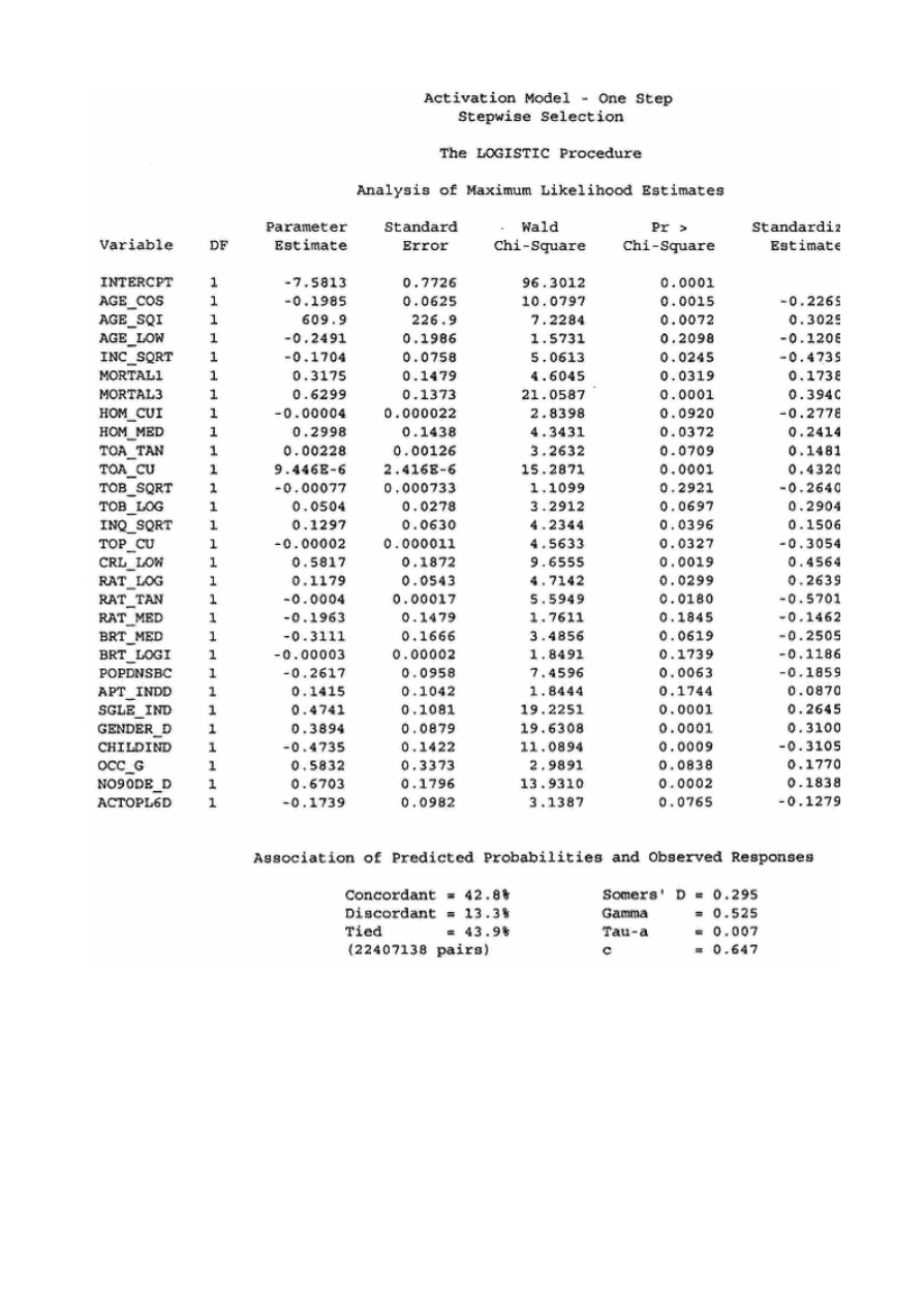
Figure

5.2

Logistic

output:

final

page

using

stepwise

method.

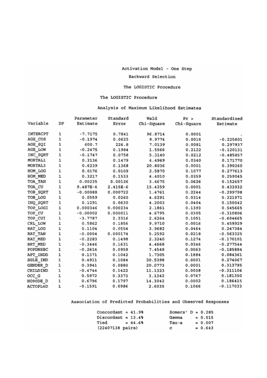
The results from the Score selection method are seen in Figure 5.4. This selection method gives us 63 variable lists, 2 for each model with 1
through 30 variables and 1 for a model with 31 variables. It also lists the overall score for the model fit. There are a number of issues to
consider when selecting the model from the list of Score. If management wants a simple model with 10 or fewer variables, then the decision
is easy. I usually start looking at about 20 variables. I examine the change in the overall score to see where adding 1 more variable can
make a big difference. For this model I select 25 variables.

Figure

5.3

Backward

selection

variable

list.ocessing

and

Evaluating

the

Model

Team-Fly

The first step in evaluating the results of the model is to look at a decile analysis. To create a decile analysis, I first sort the records by descending
model score. Then I divide the records into 10 equal groups. The statistics you choose in your table can provide a lot of information about the
predictive power of the model. The following code creates a preliminary decile analysis in SAS's PROC TABULATE. It allows us to examine how
well the model sorts our target group, the actives. I create one table using the data on which the model was built and a second one using the validation
data. But before I create the tables, I must rerun the model with the selected subset and create an output data set. The following code reruns the model
to get the estimates for the 25-variable model. It creates an output data set called acqmod.out_act1. The output data set contains a value,
predicted probability for each record. This will be used in the validation tables.

Figure

5.4

Output

from

best

subsets.

Page 114

proc logistic data=acqmod.model2(keep=
HOM_CUI AGE_COS AGE_SQI INC_SQRT MORTAL1 MORTAL3 HOM_MED TOA_TAN TOA_CU
TOB_LOG INQ_SQRT TOP_LOGI TOP_CU TOP_CUI CRL_LOW RAT_LOG BRT_MED
POPDNSBC APT_INDD SGLE_IND GENDER_D CHILDIND OCC_G NO90DE_D ACTOPL6D
respond activate pros_id active splitwgt records smp_wgt) descending;
weight splitwgt;
model active =
HOM_CUI AGE_COS AGE_SQI INC_SQRT MORTAL1 MORTAL3 HOM_MED TOA_TAN TOA_CU
TOB_LOG INQ_SQRT TOP_LOGI TOP_CU TOP_CUI CRL_LOW BRT_LOG BRT_MED
POPDNSBC APT_INDD SGLE_IND GENDER_D CHILDIND OCC_G NO90DE_D ACTOPL6D;
output out=acqmod.out_act1 pred=pred;
run;

The following code sorts the data by the predicted value pred. The descending option brings the highest predicted
probabilities to the beginning of the data set.

proc sort data=acqmod.out_act1;
by descending pred;
run;

What Is the Right Number of Variables?

I'm often asked this question! There is no right answer. I've seen models with as few as 5 variables and as
many as 100. In the case study, I looked for a point where the increased predictive power for each new
variable was tapering off. This is a good rule of thumb when you are just considering model efficiency.

In considering model performance, I think there are a few basic considerations. One argument for a specific
number of variables could be robustness. It's not clear whether a model with a large number of variables is
more robust than a model with a small number of variables. It depends on the market. With a large number
of variables, the model will be less sensitive to changes to the inputs from any one variable. If your market is
very stable, you might be better off with a large number of variables. On the other hand, if your market
behavior reflects changing trends, you might want fewer variables that capture those changes more
dynamically.

Another consideration might be processing simplicity. Unless the processing is totally automated, models
with large numbers of variables are more prone to errors in scoring.

And finally, business issues can determine the best number of variables. If companies want to avoid biased
selections based on certain demographics, a higher number of variables would spread the effect. On the other
hand, some managers are more comfortable with fewer variables because they can understand the
components that are driving the model. Business knowledge and experience are your best guide.

Page 115

The following code calculates the total sum of the weights, sumwgt, in the data set. The goal is to divide the data set into
10 equal groups or deciles. By creating deciles of the file, sorted by probabilities of becoming active, we can evaluate
how well the model score pulls the true actives (active = 1) to the best decile (decile 0).

There are several other methods for creating deciles within the SAS system. PROC RANK is a procedure designed for
that purpose. Another technique is to use the decile identifiers available from PROC UNIVARIATE. Both PROC
RANK and PROC UNIVARIATE use values to identify the decile cutoffs. Because I am using a sample with weights,
there are many groups that have the same exact probability. And using those techniques everyone with the same
probability goes into the same decile. Therefore, it is difficult to create deciles of equal size.

proc univariate data=acqmod.out_act1
(where=( splitwgt =.)) noprint;
weight smp_wgt;
var pred active;
output out=preddata sumwgt=sumwgt;
run;

The following code appends the sumwgt or the weighted total number of records to the file and creates a new data set
with only the model data (where splitwgt =1). Next, a variable is created called number that assigns a unique value to
each observation in order of predicted probability to become active. The deciles are created using cutoffs at each tenth of
the file. And finally, a variable, activ_r, is created that represents a numeric form of activate. This is used in the table
below.

/* DECILE CREATION */
data acqmod.mod_dec;
set acqmod.out_act1 (where=( splitwgt =.));
if (_n_ = 1) then set preddata;
retain sumwgt;
number+smp_wgt;
if number < .1*sumwgt then mod_dec = 0; else
if number < .2*sumwgt then mod_dec = 1; else
if number < .3*sumwgt then mod_dec = 2; else
if number < .4*sumwgt then mod_dec = 3; else
if number < .5*sumwgt then mod_dec = 4; else
if number < .6*sumwgt then mod_dec = 5; else
if number < .7*sumwgt then mod_dec = 6; else
if number < .8*sumwgt then mod_dec = 7; else
if number < .9*sumwgt then mod_dec = 8; else
mod_dec = 9;
activ_r = (activate = '1');
run;

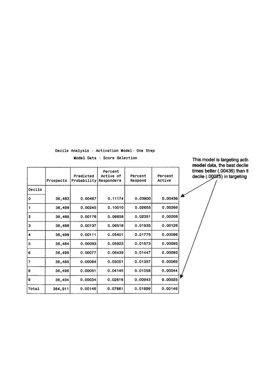
The following code uses PROC TABULATE to create the decile analysis, a table that calculates the number of observations (records) in
each decile, the average predicted probability per decile, the percent active per responders (target of Method 2, model 2), the response
rate (target of Method 2, model 1), and the active rate (target of Method 1).

title1 "Decile Analysis - Activation Model - One Step";
title2 "Model Data - Score Selection";
proc tabulate data=acqmod.mod_dec;
weight smp_wgt;
class mod_dec;
var respond active pred records activ_r;
table mod_dec='Decile' all='Total',
records='Prospects'*sum=' '*f=comma10.
pred='Predicted Probability'*(mean=' '*f=11.5)
activ_r='Percent Active of Responders'*(mean=' '*f=11.5)
respond='Percent Respond'*(mean=' '*f=11.5)
active='Percent Active'*(mean=' '*f=11.5)
/rts = 9 row=float;
run;

In Figure 5.5, the decile analysis shows the model's ability to rank order the prospects by their active behavior. To clarify, each
prospect's probability of becoming active is considered its rank. The goal of the model is to rank order the prospects so as to bring the
true actives to the lowest decile. At first glance we can see that the best decile (0) has 17.5 as many actives as the worst decile

Figure

5.5

Decile

analysis

using

model

data.

Page 117

(9). And as we go from decile 0 to decile 9, the percent active value is monotonically decreasing with a strong decrease
in the first three deciles. The only exception is the two deciles in the middle with the same percent active rate. This is not
unusual since the model is most powerful in deciles 0 and 9, where it gets the best separation. Overall, the model score
does a good job of targeting active accounts. Because the model was built on the data used in Figure 5.5, a better test
will be on the validation data set.

Another consideration is how closely the ''Percent Active" matches the "Predicted Probability." The values in these
columns for each decile are not as close as they could be. If my sample had been larger, they would probably be more
equal. I will look for similar behavior in the decile analysis for the validation data set.

Preliminary Evaluation

Because I carried the validation data through the model using the missing weights, each time the model is processed, the
validation data set is scored along with the model data. By creating a decile analysis on the validation data set we can
evaluate how well the model will transfer the results to similar data. As mentioned earlier, a model that works well on
alternate data is said to be robust. In chapter 6, I will discuss additional methods for validation that go beyond simple
decile analysis.

The next code listing creates the same table for the validation data set. This provides our first analysis of the ability of
the model to rank order data other than the model development data. It is a good test of the robustness of the model or its
ability to perform on other prospect data. The code is the same as for the model data decile analysis except for the
(where=( splitwgt = .)) option. This accesses the "hold out" sample or validation data set.

proc univariate data=acqmod.out_act1
(where=( splitwgt = .)) noprint;
weight smp_wgt;
var pred active;
output out=preddata sumwgt=sumwgt;
run;

data acqmod.val_dec;
set acqmod.out_act1(where=( splitwgt = .)) ;
if (_n_ eq 1) then set preddata;
retain sumwgt;
number+smp_wgt;
if number < .1*sumwgt then val_dec = 0; else
if number < .2*sumwgt then val_dec = 1; else
if number < .3*sumwgt then val_dec = 2; else
if number < .4*sumwgt then val_dec = 3; else

if number < .5*sumwgt then val_dec = 4; else
if number < .6*sumwgt then val_dec = 5; else
if number < .7*sumwgt then val_dec = 6; else
if number < .8*sumwgt then val_dec = 7; else
if number < .9*sumwgt then val_dec = 8; else
val_dec = 9;
activ_r = (activate = '1');
run;

title1 "Decile Analysis - Activation Model - One Step";
title2 "Validation Data - Score Selection";
PROC tabulate data=acqmod.val_dec;
weight smp_wgt;
class val_dec;
var respond active pred records activ_r;
table val_dec='Decile' all='Total',
records='Prospects'*sum=' '*f=comma10.
pred='Predicted Probability'*(mean=' '*f=11.5)
activ_r='Percent Active of Responders'*(mean=' '*f=11.5)
respond='Percent Respond'*(mean=' '*f=11.5)
active='Percent Active'*(mean=' '*f=11.5)
/rts = 9 row=float;
run;

The validation decile analysis seen in Figure 5.6 shows slight degradation from the original model. This is to be expected. But the rank
ordering is still strong

Figure

5.6

Decile

analysis

using

validation

data.

Page 119

with the best decile attracting almost seven times as many actives as the worst decile. We see the same degree of
difference between the "Predicted Probability" and the actual "Percent Active" as we saw in the decile analysis of the
model data in Figure 5.5. Decile 0 shows the most dramatic difference, but the other deciles follow a similar pattern to
the model data. There is also a little flipflop going on in deciles 5 and 6, but the degree is minor and probably reflects
nuances in the data. In chapter 6, I will perform some more general types of validation, which will determine if this is a
real problem.

Method 2:
Two Models — Response

The process for two models is similar to the process for the single model. The only difference is that the response and
activation models are processed separately through the stepwise, backward, and Score selection methods. The code
differences are highlighted here:

proc logistic data=acqmod.model2
(keep=variables) descending;
weight splitwgt;
model respond = variables
/selection = stepwise sle=.3 sls=.3;
run;
proc logistic data=acqmod.model2
(keep=variables) descending;
weight splitwgt;
model respond = variables
/selection = backward sls=.3;
run;

proc logistic data=acqmod.model2
(keep=variables) descending;
weight splitwgt;
model respond = variables
/selection = score best=2;
run;

The output from the Method 2 response models is similar to the Method 1 approach. Figure 5.7 shows the decile analysis
for the response model calculated on the validation data set. It shows strong rank ordering for response. The rank
ordering for activation is a little weaker, which is to be expected. There are different drivers for response and activation.
Because activation is strongly driven by response, the ranking for activation is strong.

Method 2:
Two Models — Activation

As I process the model for predicting activation given response (active|response), recall that I can use the value activate
because it has a value of missing for nonresponders. This means that the nonresponders will be eliminated from the
model processing. The following code processes the model:

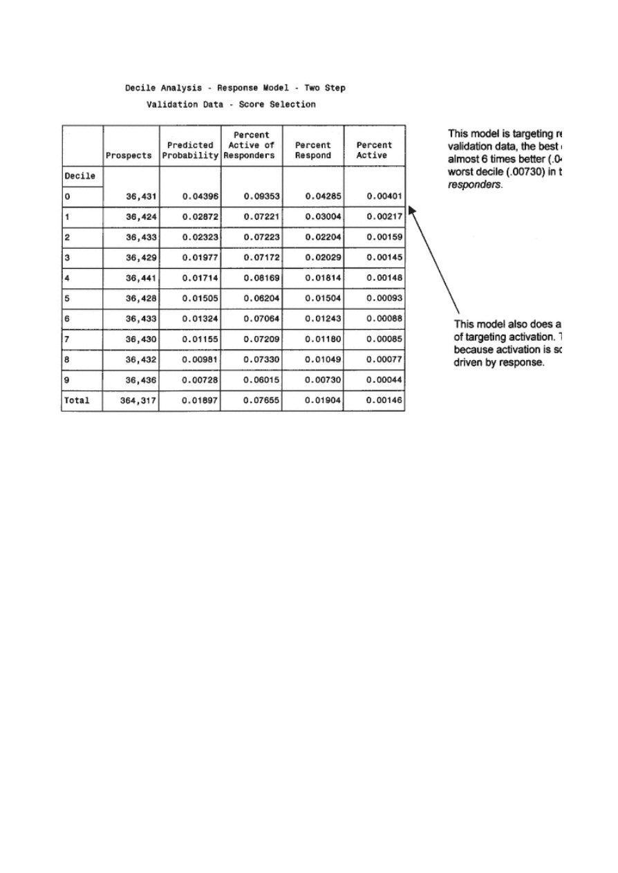
Figure

5.7

Method

response

model

decile

analysis.

proc logistic data=acqmod.model2
(keep=variables) descending;
weight splitwgt;
model activate = variables
/selection = stepwise sle=.3 sls=.3;
run;

proc logistic data=acqmod.model2
(keep=variables) descending;
weight splitwgt;
model activate = variables
/selection = backward sls=.3;
run;

proc logistic data=acqmod.model2
(keep=variables) descending;
weight splitwgt;
model activate = variables
/selection = score best=2;
run;

The output from the Method 2 activation models is similar to the Method 1 approach. Figure 5.8 shows the decile analysis for the activation
model calculated on the validation data set. It shows strong rank ordering for activation given response. As expected, it is weak when
predicting activation for the entire file. Our next step is to compare the results of the two methods.

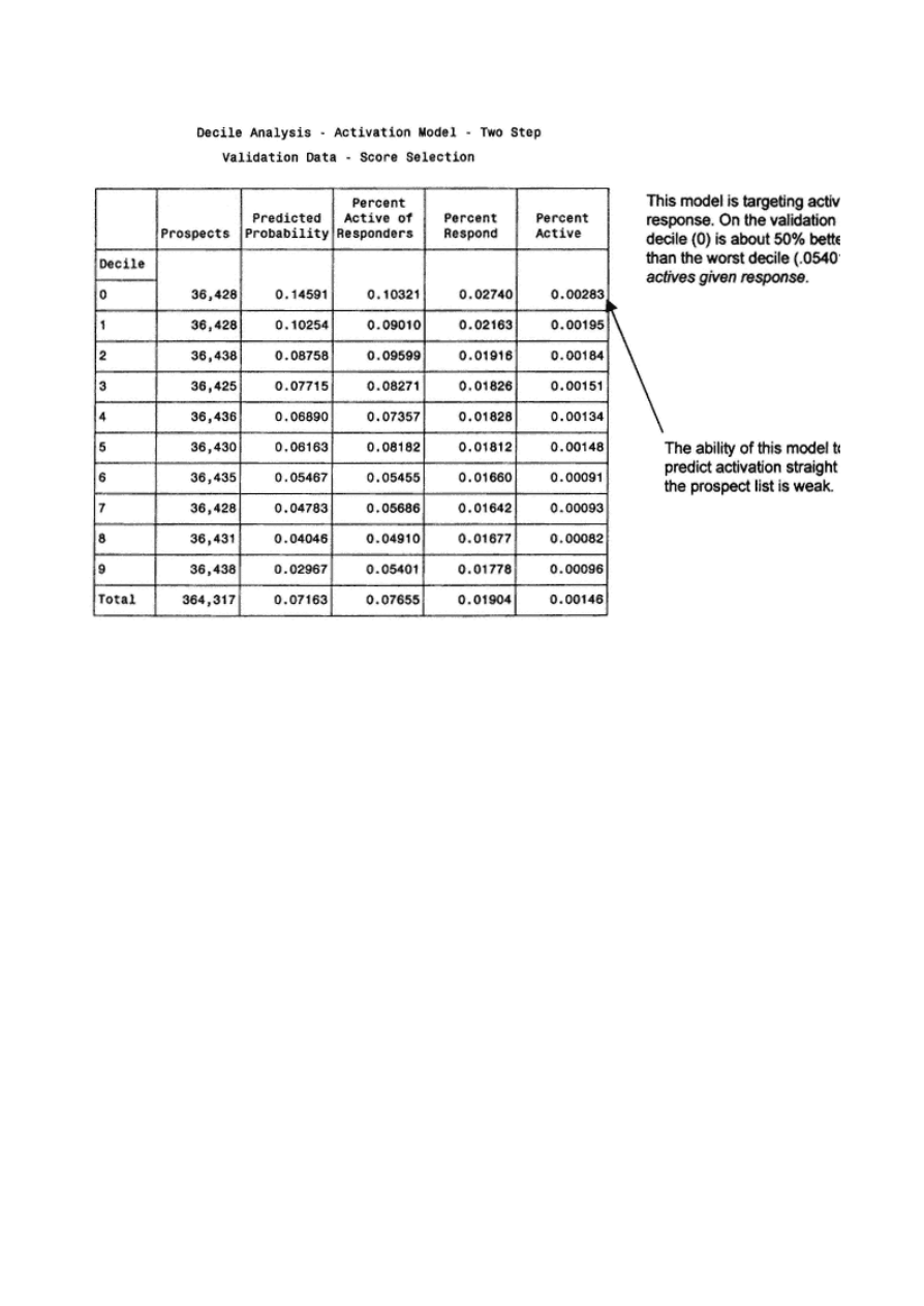
Figure

5.8

Method

activation

model

decile

analysis.

Comparing Method 1 and Method 2

At this point, I have several options for the final model. I have a single model that predicts the probability of an active account that was
created using Method 1, the single -model approach. And I have two models from Method 2, one that predicts the probability of response
and the other that predicts the probability of an active account, given response (active|response).

To compare the performance between the two methods, I must combine the models developed in Method 2. To do this, I use a simplified
form of Bayes' Theorem. Let's say:

P(R) = the probability of response (model 1 in Method 2)

P(A|R) = the probability of becoming active given response (model 2 in Method 2)

P(A and R) = the probability of responding and becoming active

Then:

P(A and R) = P(R)* P(A|R)

Therefore, to get the probability of responding and becoming active, I multiply the probabilities created in model 1 and model 2.

Team-Fly

Page 122

Following the processing of the score selection for each of the two models in Method 2, I reran the models with the final
variables and created two output data sets that contained the predicted scores, acqmod.out_rsp2 and acqmod.out_act2.
The following code takes the output data sets from the Method 2 models built using the score option. The where=
( splitwgt = .) option designates both probabilities are taken from the validation data set. Because the same sample was
used to build both models in Method 2, when merged together by pros_id the names should match up exactly. The
rename=(pred=predrsp) creates different names for the predictors for each model.

proc sort data=acqmod.out_rsp2 out=acqmod.validrsp
(where=( splitwgt = .) rename=(pred=predrsp)) ;
by pros_id;
run;

proc sort data=acqmod.out_act2 out=acqmod.validact
(where=( splitwgt = .) rename=(pred=predact)) ;
by pros_id;
run;

data acqmod.blend;
merge acqmod.validrsp acqmod.validact;
by pros_id;
run;

data acqmod.blend;
set acqmod.blend;
predact2 = predrsp*predact;
run;

To compare the models, I create a decile analysis for the probability of becoming active derived using Method 2
(predact2 ) with the following code:

proc sort data=acqmod.blend;
by descending predact2;
run;

proc univariate data=acqmod.blend noprint;
weight smp_wgt;
var predact2;
output out=preddata sumwgt=sumwgt;
run;

data acqmod.blend;
set acqmod.blend;
if (_n_ eq 1) then set preddata;
retain sumwgt;
number+smp_wgt;
if number < .1*sumwgt then act2dec = 0; else

Page 123

if number < .2*sumwgt then act2dec = 1; else
if number < .3*sumwgt then act2dec = 2; else
if number < .4*sumwgt then act2dec = 3; else
if number < .5*sumwgt then act2dec = 4; else
if number < .6*sumwgt then act2dec = 5; else
if number < .7*sumwgt then act2dec = 6; else
if number < .8*sumwgt then act2dec = 7; else
if number < .9*sumwgt then act2dec = 8; else
act2dec = 9;
run;

title1 "Decile Analysis - Model Comparison";
title2 "Validation Data - Two Step Model";
PROC tabulate data=acqmod.blend;
weight smp_wgt;
class act2dec;
var active predact2 records;
table act2dec='Decile' all='Total',
records='Prospects'*sum=' '*f=comma10.
predact2='Predicted Probability'*(mean=' '*f=11.5)
active='Percent Active'*(mean=' '*f=11.5)
/rts = 9 row=float;
run;

In Figure 5.9, the decile analysis of the combined scores on the validation data for the two -model approach shows a
slightly better performance than the one -model approach in Figure 5.6. This provides confidence in our results. At first
glance, it's difficult to pick the winner.

Figure

5.9

Combined

model

decile

analysis.

Page 124

Summary

This chapter allowed us to enjoy the fruits of our labor. I built several models with strong power to rank order the
prospects by their propensity to become active. We saw that many of the segmented and transformed variables
dominated the models. And we explored several methods for finding the best-fitting model using two distinct
methodologies. In the next chapter, I will measure the robustness of our models and select a winner.

Page 125

Chapter 6—
Validating the Model

The masterpiece is out of the oven! Now we want to ensure that it was cooked to perfection. It's time for the taste test!

Validating the model is a critical step in the process. It allows us to determine if we've successfully performed all the
prior steps. If a model does not validate well, it can be due to data problems, poorly fitting variables, or problematic
techniques. There are several methods for validating models. In this chapter, I begin with the basic tools for validating
the model, gains tables and gains charts. Marketers and managers love them because they take the modeling results right
to the bottom line. Next, I test the results of the model algorithm on an alternate data set. A major section of the chapter
focuses on the steps for creating confidence intervals around the model estimates using resampling. This is gaining
popularity as an excellent method for determining the robustness of a model. In the final section I discuss ways to
validate the model by measuring its effect on key market drivers.

Gains Tables and Charts

A gains table is an excellent tool for evaluating the performance of a model. It contains actionable information that can
be easily understood and used by non-

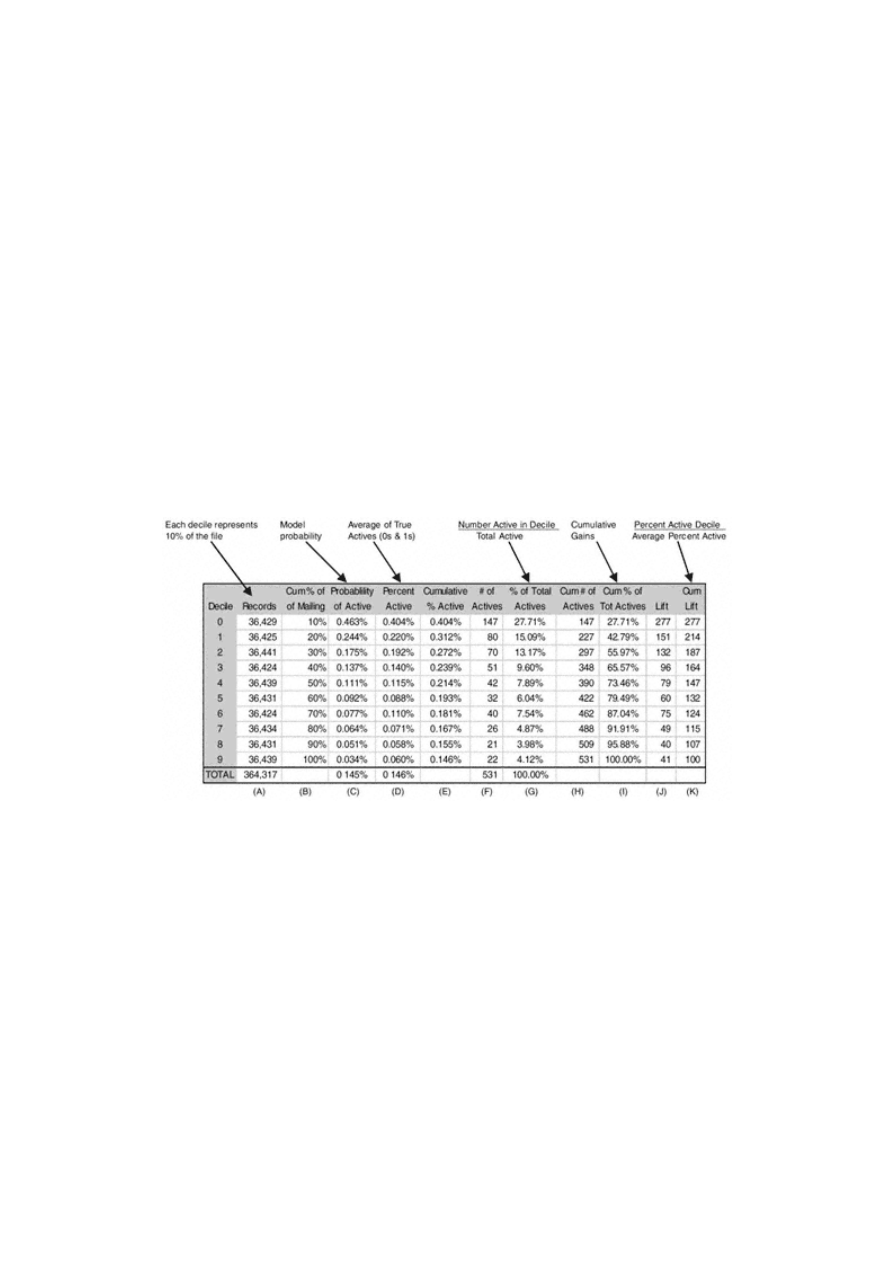
Page 126

technical marketers and managers. Using our case study, I will demonstrate the power of a gains table for Method 1.

Method 1:
One Model

Recall that in Method 1 I developed a score for targeting actives using the one-model approach. To further validate the
results of the model, I put the information from the decile analysis in Figure 5.6 into a spreadsheet; now I can create the
gains table in Figure 6.1.

Column A mirrors the decile analysis in Figure 5.6. It shows each decile containing 10% of the total mail file.

Column B is cumulative percent of file for validation portion of the prospect data set.

Column C, as in Figure 5.6, is the average Probability of Activation for each decile as defined by the model.

Column D, as in Figure 5.6, is the average Percent Actives in the validation data set for each decile. This represents the
number of true actives in the validation data set divided by the total prospects for each decile.

Column E is a cumulative calculation of column D or Cumulative Percent Actives. At each decile you can estimate the
number of true actives for a given "Depth of File" or from decile 0 to a designated decile. If we consider the value for
decile 4, we can say that the average Percent Active for deciles 0 through 4 is 0.214%.

Column F is the number of true actives in the decile (Col. A * Col. D).

Figure

6.1

Enhanced

gains

table

validation

data.alidating

the

Model

Page 127

Column G is column F divided by the sum of column F. This represents the percent Actives of the Total Actives that are
contained in each decile. If we consider the value in Decile 1, we can say that 27.71% of all Actives in the validation
data set were put into decile 1 by the model.

Column H is a cumulative of column F. This represents the total Number of Actives for a given ''Depth of File" or from
decile 0 to a designated decile.

Column I is column H divided by the number of total actives. At each decile you can determine the Cumulative Percent
of Total Actives that are contained in decile 0 through a given decile. If we consider the value in decile 1, we can say that
42.79% of all Actives are in deciles 0 and 1.

Column J is the "lift" of each decile. The lift is calculated by dividing the decile percent active by the overall percent
active in column D. The value of 277 in decile 0 means that the prospects in decile 0 are 277% more likely to activate
than the overall average.

Column K is the cumulative Lift through a specific decile. It is calculated by dividing a decile value in column E by the
overall percent active.

The lift measurement is a favorite among marketers for evaluating and comparing models. At each decile it demonstrates
the model's power to beat the random approach or average performance. In Figure 6.1, we see that decile 0 is 2.77 times
the average. Up to and including decile 3, the model performs better than average. Another way to use lift is in
cumulative lift . This means to a given "Depth of File": the model performs better than random. If we go through decile 3,
we can say that for the first four deciles, the model performs 64% better than average. Figure 6.2, a validation gains
chart, provides a visual interpretation of the concept of Lift.

The gains chart is an excellent visual tool for understanding the power of a model. It is designed to compare the percent
of the target group to the percent of the prospect file through the rank ordered data set. At 50% of the file we can capture
74% of the active accounts— a 47% increase in Actives. (This will be discussed in more detail in chapter 7.)

Method 2:
Two Models

Recall that in Method 2, I built a model to target Response and a second model to target Actives given response.

In Figure 6.3 we see the ability of the Method 2 model to rank order the data. When comparing the active rate for the
deciles, the power of the model is slightly better than the Method 1 model in distinguishing actives from nonresponders
and nonactive responders. The lift measures imitate the similarity.

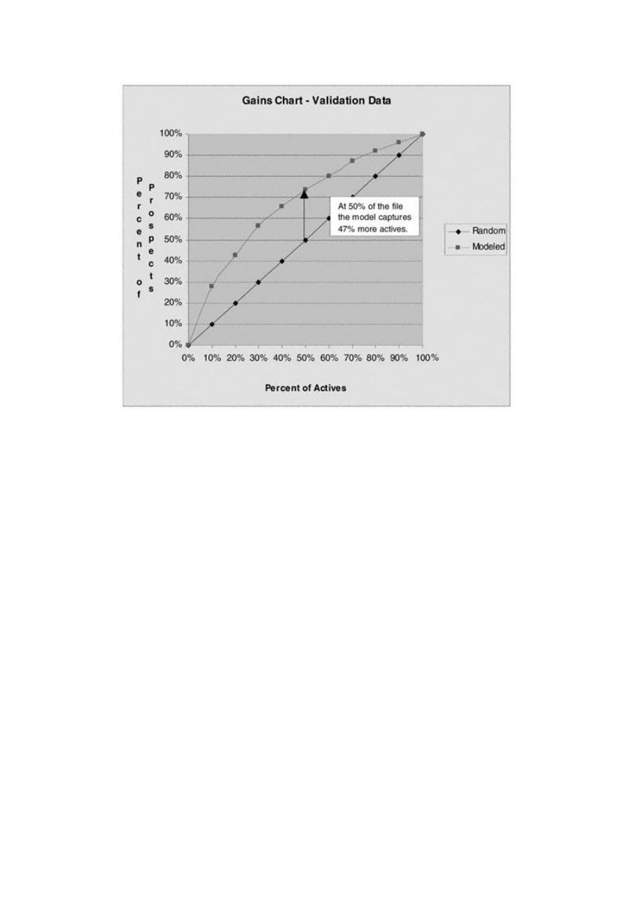
Page 128

Figure

6.2

Validation

gains

chart.

Recall that the response model in the two-model approach did a good job of predicting actives overall. The gains chart in
Figure 6.4 compares the activation model from the one -model approach to the response and combination models
developed using the two-model approach. The response model seems to do almost as well as the active models. Again,
this supports our theory that the probability of being active is strongly driven by response.

In conclusion, Method 1 and Method 2 produce very similar results when modeling the probability of an account being
active. This may not always be the case. It is worth exploring both methods to determine the best method for each
situation. In the next sections, I will compare the stability of the models through further validation. In chapter 7, I will
discuss alternate ways to use the Method 2 models in the implementation process.

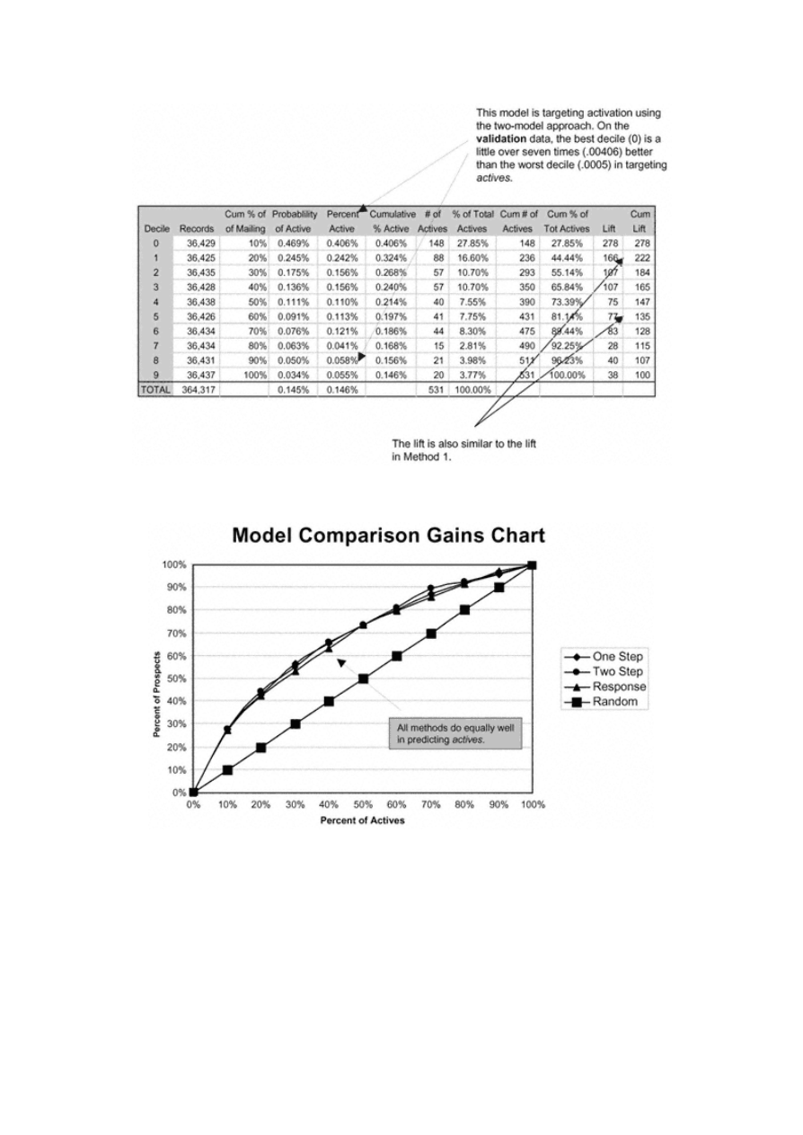
Page 129

Figure

6.3

Enhanced

gains

table

validation

data.

Figure

6.4

Gains

chart

comparing

models

from

Method

and

Method

Page 130

Scoring Alternate Data Sets

In business, the typical purpose of developing a targeting model is to predict behavior on a data set other than that on
which the model was developed. In our case study, I have our "hold out" sample that I used for validation. But because it
was randomly sampled from the same data set as the model development data, I expect it to deliver a performance very
similar to that of the model development data. The best way to test the robustness of the model is to score a campaign
that more closely reflects the intended use. For example, a similar campaign from a different time period is optimal
because most models are designed for future use in the same general market. Other options include campaigns from
different geographic regions or for a slightly different product.

Our case study deals with the insurance industry, which is highly regulated. Therefore, it is quite common to begin
marketing in just one or two states. Expansion typically happens on a state-by-state basis. For our case study, the goal is
to use the model for name selection in a new state with the hope of improving on random selection. Our model was
developed on a campaign in the state of New York. Now I will validate the scoring algorithm on the results from the
state of Colorado.

I will concentrate on the Method 1 approach for this validation because the mechanics and results should be similar. The
same processing will be performed on the Method 2 combined model for comparison. The first step is to read in the data
from the Colorado campaign. The input statement is modified to read in only the necessary variables.

data acqmod.colorado;
infile 'F:\insur\acquisit\camp3.txt' missover recl=99;
input
prosp_id 1-9 /*unique prospect identifier*/
pop_den $ 13 /*population density code*/
| | | | |
| | | | |
no90eve 97-99 /*number of payments over 90 days */
;
run;

The next step is to create the variable transformations needed for the model scoring. The code is a reduced version of the
code used in chapter 4 to create the original variables so it won't be repeated here. I rerun the logistic model on the
original (New York) data to create a data set with one observation using outest=acqmod.nyscore . This data set contains
the coefficients of the model. The output from acqmod.nyscore is seen in Figure 6.5.

Figure

6.5

Coefficient

data

set.

proc logistic data=acqmod.colorado descending
outest=acqmod.nyscore;
weight splitwgt;
model active =
HOM_CUI AGE_COS AGE_SQI INC_SQRT MORTAL1 MORTAL3 HOM_MED TOA_TAN TOA_CU
TOB_LOG INQ_SQRT TOP_LOGI TOP_CU TOP_CUI CRL_LOW RAT_LOG BRT_MED
POPDNSBC APT_INDD SGLE_IND GENDER_D CHILDIND OCC_G NO90DE_D ACTOPL6D;
run;

proc print data = acqmod.nyscore;
run;

The final scoring is carried out using PROC SCORE. The procedure multiplies the coefficients in the model from (acqmod.nyscore
values in the data set to be scored (acqmod.colorado) and creates a new data set (acqmod.validco), which contains the estimates or betas for each
observation. The line beginning with 'id' brings additional variables into the scored data set.

proc score data=acqmod.colorado
out=acqmod.validco predict score=acqmod.nyscore type=parms;
id respond activate pros_id activ_r activate splitwgt records smp_wgt;
VAR HOM_CUI AGE_COS AGE_SQI INC_SQRT MORTAL1 MORTAL3 HOM_MED TOA_TAN
TOA_CU TOB_LOG INQ_SQRT TOP_LOGI TOP_CU TOP_CUI CRL_LOW RAT_LOG BRT_MED
POPDNSBC APT_INDD SGLE_IND GENDER_D CHILDIND OCC_G NO90DE_D ACTOPL6D;
run;

The output for PROC SCORE gives us the sum of the betas. Recall from chapter 1 that we use it in the following equation to calculate the
probability:

The rank ordering for the estimate and the predicted probability (pred) are the same. I sort the file by descending estimate and find the sum of the weights
(sumwgt) to create a decile analysis.

Team-Fly

Page 132

proc sort data=acqmod.validco;
by descending estimate;
run;

proc univariate data=acqmod.validco noprint;
weight smp_wgt;
var estimate;
output out=preddata sumwgt=sumwgt;
run;

data acqmod.validco;
set acqmod.validco;
active = (activate='1');
pred = exp(estimate)/(1+exp(estimate));
if (_n_ eq 1) then set preddata;
retain sumwgt;
number+smp_wgt;
if number < .1*sumwgt then val_dec = 0; else
if number < .2*sumwgt then val_dec = 1; else
if number < .3*sumwgt then val_dec = 2; else
if number < .4*sumwgt then val_dec = 3; else
if number < .5*sumwgt then val_dec = 4; else
if number < .6*sumwgt then val_dec = 5; else
if number < .7*sumwgt then val_dec = 6; else
if number < .8*sumwgt then val_dec = 7; else
if number < .9*sumwgt then val_dec = 8; else
val_dec = 9;
records = 1;
run;

title1 "Gains Table - Colorado";
title2 "Validation Data";
PROC tabulate data=acqmod.validco;
weight smp_wgt;
class val_dec;
var respond active pred records activ_r;
table val_dec='Decile' all='Total',
records='Prospects'*sum=' '*f=comma10.
pred='Predicted Probability'*(mean=' '*f=11.5)
active='Percent Active'*(mean=' '*f=11.5)
/rts = 9 row=float;
run;

In Figure 6.6, we see that the Method 1 model does show a loss of power when scored on the campaign from another
state. This is probably due to some population differences between states. Figure 6.7 shows similar results from the
Method 2 model. In any case, the performance is still much better than random with the best decile showing three times
the active rate of the worst decile.

Page 133

Figure

6.6

Alternate

state

gains

table— Method

Figure

6.7

Alternate

state

gains

table— Method

Page 134

Therefore, in the typical application this type of model would be very efficient in reducing the costs related to entering a
new state. The model could be used to score the new state data. The best approach is to mail the top two or three deciles
and sample the remaining deciles. Then develop a new model with the results of the campaign.

At this point the Method 1 model and the Method 2 model are running neck and neck. The next section will describe
some powerful tools to test the robustness of the models and select a winner.

Resampling

Resampling is a common-sense, nonstatistical technique for estimating and validating models. It provides an empirical
estimation (based on experience and observation) instead of a parametric estimation (based on a system or distribution).
Consider the basic premise that over-fitting is fitting a model so well that it is picking up irregularities in the data that
may be unique to that particular data set. In model development, resampling is commonly used in two ways: (1) it avoids
over-fitting by calculating model coefficients or estimates based on repeated sampling; or (2) it detects over-fitting by
using repeated samples to validate the results of a model. Because our modeling technique is not prone to over-fitting the
data, I will focus on the use of resampling as a validation technique. This allows us to calculate confidence intervals
around our estimates.

Two main types of resampling techniques are used in database marketing: jackknifing and bootstrapping. The following
discussion and examples highlight and compare the power of these two techniques.

Jackknifing

In its purest form, jackknifing is a resampling technique based on the "leave -one-out" principle. So, if N is the total
number of observations in the data set, jackknifing calculates the estimates on N – 1 different samples each having N – 1
observations. This works well for small data sets. In model development, though, we are dealing with large data sets that
can be cumbersome to process. A variation of the jackknifing procedure works well on large data sets. It works on the
same principle as leave-one-out. Instead of just one record, it leaves out a group of records. Overall, it gives equal
opportunity to every observation in the data set.

In our case study, the model was developed on a 50% random sample, presumed to be representative of the entire
campaign data set. A 50% random sample was held out for validation. In this section, I use jackknifing to estimate the
pre-

Page 135

dicted probability of active, the actual active rate, and the lift for each decile using 100–99% samples. I will show the
code for this process for the Method 1 model. The process will be repeated for the Method 2 model, and the results will
be compared.

The program begins with the logistic regression to create an output file (acqmod.resamp) that contains only the
validation data and a few key variables. Each record is scored with a predicted value (pred).

proc logistic data=acqmod.model2 descending;
weight splitwgt;
model active =HOM_CUI AGE_COS AGE_SQI INC_SQRT MORTAL1 MORTAL3 HOM_MED
TOA_TAN TOA_CU TOB_LOG INQ_SQRT TOP_LOGI TOP_CU TOP_CUI CRL_LOW RAT_LOG
BRT_MED POPDNSBC APT_INDD SGLE_IND GENDER_D CHILDIND OCC_G NO90DE_D
ACTOPL6D;
output out=acqmod.resamp(where=(splitwgt=.) keep=pred active records
smp_wgt splitwgt) pred=pred;
run;

The following code begins a macro that creates 100 jackknife samples. Using a do loop, each iteration eliminates 1% of
the data. This is repeated 100 times. The ranuni (5555) function with the positive seed (5555) ensures the same random
number assignment for each iteration of the do loop. The resulting samples each have a different 1% eliminated.

%macro jackknif;
%do prcnt = 1 %to 100;
data acqmod.outk&prcnt;
set acqmod.resamp;
if .01*(&prcnt-1) < ranuni(5555) < .01*(&prcnt) then delete;
run;

The following code is similar to that in chapter 5 for creating deciles. In this case, this process is repeated 100 times to
create 100 decile values. The value &prcnt increments by 1 during each iteration.

proc sort data=acqmod.outk&prcnt;
by descending pred;
run;

proc univariate data=acqmod. outk&prcnt noprint;
weight smp_wgt;
var pred;
output out=preddata sumwgt=sumwgt;
run;

data acqmod.outk&prcnt;
set acqmod.outk&prcnt;
if (_n_ eq 1) then set preddata;

Page 136

retain sumwgt;
number+smp_wgt;
if number < .1*sumwgt then val_dec = 0; else
if number < .2*sumwgt then val_dec = 1; else
if number < .3*sumwgt then val_dec = 2; else
if number < .4*sumwgt then val_dec = 3; else
if number < .5*sumwgt then val_dec = 4; else
if number < .6*sumwgt then val_dec = 5; else
if number < .7*sumwgt then val_dec = 6; else
if number < .8*sumwgt then val_dec = 7; else
if number < .9*sumwgt then val_dec = 8; else
val_dec = 9;
run;

In proc summary, the average values for active rate (actmn&samp) and predicted probability (prdmn&samp) are
calculated for each decile. This is repeated and incremented 100 times; 100 output data sets (jkmns&prcnt ) are created
with the average values.

proc summary data=acqmod. outk&prcnt;
var active pred;
class val_dec;
weight smp_wgt;
output out=acqmod. jkmns&prcnt mean=actmn&prcnt prdmn&prcnt;
run;

To calculate the lift for each decile, the value for the overall predicted probability of active and the actual active rate are
needed. These are extracted from the output file from proc summary. There is one observation in the output data set
where the decile value (val_dec) is missing (.). That represents the overall means for each requested variable.

data actomean(rename=(actmn&prcnt=actom&prcnt) drop=val_dec);
set acqmod.jkmns&prcnt(where=(val_dec=.) keep=actmn&prcnt val_dec);
run;

The overall values are appended to the data sets and the lifts are calculated.

data acqmod.jkmns&prcnt;
set acqmod.jkmns&prcnt;
if (_n_ eq 1) then set actomean;
retain actom&prcnt;
liftd&prcnt = 100*actmn&prcnt/actom&prcnt;

After this process is repeated 100 times, the macro is terminated.

%end;
%mend;

%jackknif;

Page 137

The 100 output files are merged together by decile. The values for the mean and standard deviation are calculated for the
predicted probability of active, the actual active rate, and the lift. The corresponding confidence intervals are also
calculated.

data acqmod.jk_sum(keep = prdmjk lci_p uci_p
actmjk lci_a uci_a lftmjk lci_l uci_l val_dec);
merge
acqmod.jkmns1 acqmod.jkmns2 acqmod.jkmns3 . . . . . . . . . . . . acqmod.jkmns99
acqmod.jkmns100;
by val_dec;
prdmjk = mean(of prdmn1 -prdmn100); /* predicted probability */
prdsdjk = std(of prdmn1 -prdmn100);

actmjk = mean(of actmn1 -actmn100); /* active rate */
actsdjk = std(of actmn1 -actmn100);

lftmjk = mean(of liftd1 -liftd100); /* lift on active rate */
lftsdjk = std(of liftd1 -liftd100);

lci_p = prdmjk - 1.96*actsdjk; /* confidence itnerval on predicted */
uci_p = prdmjk + 1.96*actsdjk;

lci_a = actmjk - 1.96*actsdjk; /* confidence itnerval on actual */
uci_a = actmjk + 1.96*actsdjk;

lci_l = lftmjk - 1.96*lftsdjk; /* confidence itnerval on lift */
uci_l = lftmjk + 1.96*lftsdjk;
run;

Proc format and proc tabulate create the gains table for validating the model. Figure 6.8 shows the jackknife estimates,
along with the confidence intervals for the predicted probability of active, the actual active rate, and the lift.

proc format;
picture perc
low-high = '009.999%' (mult=1000000);

proc tabulate data=acqmod.jk_sum;
var prdmjk lci_p uci_p
actmjk lci_a uci_a lftmjk lci_l uci_l;
class val_dec;
table (val_dec='Decile' all='Total'),
(prdmjk='JK Est Prob'*mean=' '*f=perc.
lci_p ='JK Lower CI Prob'*mean=' '*f=perc.
uci_p ='JK Upper CI Prob'*mean=' '*f=perc.

actmjk='JK Est % Active'*mean=' '*f=perc.
lci_a ='JK Lower CI % Active'*mean=' '*f=perc.
uci_a ='JK Upper CI % Active'*mean=' '*f=perc.

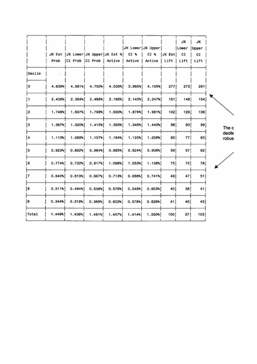
Figure

6.8

Jackknife

confidence

interval

gains

table— Method

lftmjk='JK Est Lift'*mean=' '*f=6.
lci_l ='JK Lower CI Lift'*mean=' '*f=6.
uci_l ='JK Upper CI Lift'*mean=' '*f=6.)
/rts=6 row=float;
run;

Similar processing was performed to create jackknife estimates for the Method 2 model. Figure 6.9 shows very similar results to Method 1. Figure 6.10
compares the upper and lower bounds of the confidence intervals to judge stability. Method 1 appears to provide a smoother lift curve.

Bootstrapping

Similar to jackknifing, bootstrapping is an empirical technique for finding confidence intervals around an estimate. The major difference is that
bootstrapping uses full samples of the data that are pulled from the original full sample with replacement. In other words, with a sample size of
random samples are drawn from the original sample. Because the bootstrap sample is pulled with replacement, it is possible for one observation to be
represented several

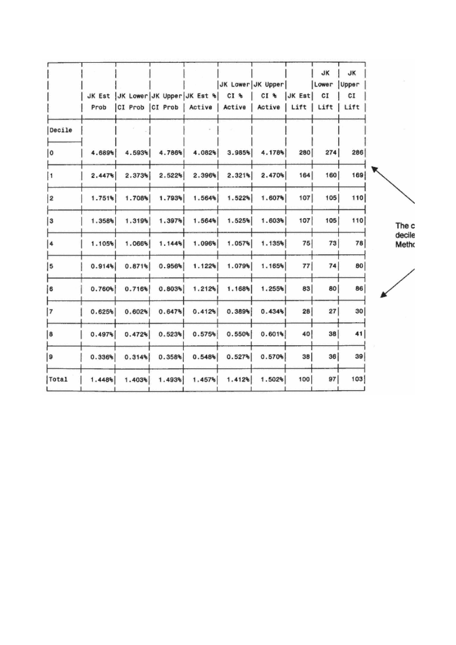
Figure

6.9

Jackknife

confidence

interval

gains

table— Method

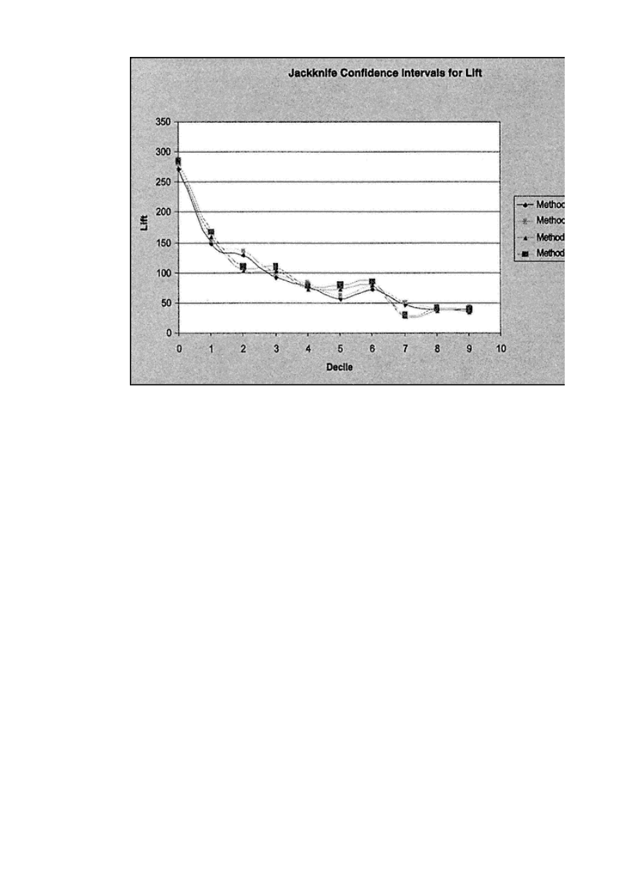
Figure

6.10

Jackknife

confidence

interval

model

comparison

graph.

Page 140

times and another observation to be missed completely. This process is repeated many times. Many industry experts
consider it a better tool for validation; however, it is more rigorous to perform.

To calculate a bootstrap confidence interval, I must first calculate the bootstrap estimate using the following
formula:

In order to calculate a confidence interval, I must derive a standard error for the bootstrap. I use the standard deviation of
the set of bootstrap estimates (BSi). A 95% bootstrap confidence intervals is derived using the following formula:

Due to the large samples in marketing data, it is often impractical and unnecessary to pull the number of samples equal
to the number of observations used in the analysis. As I did in the jackknifing example, I will modify the technique. I
begin with the same output sample that I used in the jackknifing example (acqmod.resamp). The first few steps create
decile values on the whole validation data set. This is similar to the decile analysis I created in chapter 5.

proc sort data=acqmod.resamp;
by descending pred;
run;

proc univariate data=acqmod.resamp noprint;
weight smp_wgt;
var pred active;
output out=preddata sumwgt=sumwgt mean= predmean actmean;
run;

data acqmod.resamp;
set acqmod.resamp;
if (_n_ eq 1) then set preddata;
retain sumwgt predmean actmean;
number+smp_wgt;
if number < .1*sumwgt then val_dec = 0; else
if number < .2*sumwgt then val_dec = 1; else
if number < .3*sumwgt then val_dec = 2; else
if number < .4*sumwgt then val_dec = 3; else
if number < .5*sumwgt then val_dec = 4; else
if number < .6*sumwgt then val_dec = 5; else
if number < .7*sumwgt then val_dec = 6; else
if number < .8*sumwgt then val_dec = 7; else
if number < .9*sumwgt then val_dec = 8; else
val_dec = 9;
run;

Team-Fly

Page 141

Using the decile values as class values, proc summary calculates the overall mean for the active rate and the predicted
probability for each decile. These values are used in the final bootstrap calculation.

proc summary data=acqmod.resamp;
var active pred smp_wgt;
class val_dec ;
weight smp_wgt;
output out=acqmod.fullmean mean=actmnf prdmnf ;
run;

The next two steps grab the overall mean from the data set acqmod.fullmean and attach it to every record in
acmod.fullmean . This will be used in the final lift calculation.

data actfmean(rename=(actmnf=actomn_g) drop=val_dec);
set acqmod.fullmean(where=
(val_dec=.) keep=actmnf val_dec);
run;

data acqmod.fullmean;
set acqmod.fullmean;
if (_n_ eq 1) then set actfmean;
retain actomn_g;
run;

Now I begin the bootstrap resampling process. This program is designed to pull 1/100th of the file and repeat this
process 100 times with replacement. This creates one bootstrap sample. This can be repeated hundreds of times. In
practice, though, it is unusual to find value in pulling more than 25 bootstrap samples.

The program is designed to have one macro that repeats the entire process 25 times. This process will be described in
detail as we go through the code. The second macro is embedded in the beginning of the first macro. This embedded
macro pulls the 1/100th samples using a ranuni (–1) function. The negative seed (-1) uses the time of day to assign the
random values to each observation. This ensures that each sample is independent of the prior sample or samples that
have been pulled. Each of the 100 iterations is pulled from acqmod.resamp, implying full replacement of the prior
sample.

%macro bootst25;
%do samp = 1 %to 25;

%macro bootstrp;
%do prcnt = 1 %to 100;
data acqmod.modbs&prcnt;
set acqmod.resamp;
if .01*(&prcnt-1) < ranuni(-1) < .01*(&prcnt) then output
acqmod.modbs&prcnt;
run;

Page 142

%end;
%mend;

%bootstrp

The next step combines the 100 - 1/100th samples to create the first bootstrap sample.

data acqmod.allbs&samp;
set
acqmod.modbs1 acqmod.modbs2 acqmod.modbs3 . . acqmod.modbs100;
run;

The next few steps create the deciles (val_dec) for each of the 25 bootstrap samples.

proc sort data=acqmod.allbs&samp;
by descending pred;
run;

proc univariate data=acqmod.allbs&samp noprint;
weight smp_wgt;
var pred;
output out=preddata sumwgt=sumwgt;
run;

data acqmod.allbs&samp;
set acqmod.allbs&samp;
if (_n_ eq 1) then set preddata;
retain sumwgt;
number+smp_wgt;
if number < .1*sumwgt then val_dec = 0; else
if number < .2*sumwgt then val_dec = 1; else
if number < .3*sumwgt then val_dec = 2; else
if number < .4*sumwgt then val_dec = 3; else
if number < .5*sumwgt then val_dec = 4; else
if number < .6*sumwgt then val_dec = 5; else
if number < .7*sumwgt then val_dec = 6; else
if number < .8*sumwgt then val_dec = 7; else
if number < .9*sumwgt then val_dec = 8; else
val_dec = 9;
run;

As in the jackknife example, the average values for the active rate (actmn&samp) and predicted probability
(prdmn&samp ) are calculated using proc summary.

proc summary data=acqmod.allbs&samp;
var active pred smp_wgt;
class val_dec;

Page 143

weight smp_wgt;
output out=acqmod.bsmns&samp mean=actmn&samp prdmn&samp;
run;

The following code pulls the overall mean for each sample (where= (val_dec=.)) and renames it ( actomn&samp) to
designate that it is the overall mean for the sample.

data actomean(rename=(actmn&samp=actomn&samp ) drop=val_dec);
set acqmod.bsmns&samp( where=(val_dec=.) keep=actmn&samp val_dec);
run;

The overall mean is then appended to each bootstrap sample to create the lift value (liftd&samp) for each bootstrap
sample. At this point, I have created all the values for which I want confidence intervals. The bootst25 macro iterates 25
times to create the 25 bootstrap samples.

data acqmod.bsmns&samp;
set acqmod.bsmns&samp;
if (_n_ eq 1) then set actomean;
retain actomn&samp;
liftd&samp = 100*actmn&samp/actomn&samp;
run;

%end;
%mend;

%bootst25

At this point, the macro processing is finished, and we have our 25 bootstrap samples. The following code combines the
25 bootstrap samples with the data set containing the values for the original validation sample (acqmod.fullmean) using
the decile value. It then calculates the mean and standard deviation for each estimate: active rate, predicted probability,
and lift. Following the formula for bootstrap coefficients, it concludes with calculations for the bootstrap estimates and
confidence intervals for the three estimates.

data acqmod.bs_sum(keep = liftf bsest_p prdmnf lci_p uci_p bsest_a
actmnf
lci_a uci_a bsest_l lftmbs lci_l uci_l val_dec actomn_g);
merge acqmod.bsmns1 acqmod.bsmns2 acqmod.bsmns3
. . . . . . . . . . . . . . . .acqmod.bsmns24
acqmod.bsmns25 acqmod.fullmean;
by val_dec;
prdmbs = mean(of prdmn1 -prdmn25);
prdsdbs = std(of prdmn1 -prdmn25);

actmbs = mean(of actmn1 -actmn25);
actsdbs = std(of actmn1 -actmn25);

Page 144

lftmbs = mean(of liftd1 -liftd25);
lftsdbs = std(of liftd1 -liftd25);

liftf = 100*actmnf/actomn_g;

bsest_p = 2*prdmnf - prdmbs;
lci_p = bsest_p - 1.96*actsdbs;
uci_p = bsest_p + 1.96*actsdbs;

bsest_a = 2*actmnf - actmbs;
lci_a = bsest_a - 1.96*actsdbs;
uci_a = bsest_a + 1.96*actsdbs;

bsest_l = 2*liftf - lftmbs;
lci_l = bsest_l - 1.96*lftsdbs;
uci_l = bsest_l + 1.96*lftsdbs;
run;

Finally, the code that follows produces the gains table seen in Figure 6.11. The results are very similar to the results seen
using the jackknifing technique. The range of values around all the estimates are fairly close, indicating a robust model.

proc format;
picture perc
low-high = '09.999%' (mult=1000000);

proc tabulate data=acqmod.bs_sum;
var liftf bsest_p prdmnf lci_p uci_p bsest_a actmnf
lci_a uci_a bsest_l lftmbs lci_l uci_l;
class val_dec;
table (val_dec='Decile' all='Total'),
(prdmnf='Actual Prob'*mean=' '*f=perc.
bsest_p='BS Est Prob'*mean=' '*f=perc.
lci_p ='BS Lower CI Prob'*mean=' '*f=perc.
uci_p ='BS Upper CI Prob'*mean=' '*f=perc.

actmnf ='Percent Active'*mean=' '*f=perc.
bsest_a='BS Est % Active'*mean=' '*f=perc.
lci_a ='BS Lower CI % Active'*mean=' '*f=perc.
uci_a ='BS Upper CI % Active'*mean=' '*f=perc.

liftf ='Lift'*mean=' '*f=4.
bsest_l='BS Est Lift'*mean=' '*f=4.
lci_l ='BS Lower CI Lift'*mean=' '*f=4.
uci_l ='BS Upper CI Lift'*mean=' '*f=4.)
/rts=6 row=float;
run;

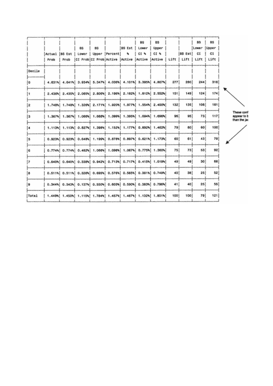
Figure

6.11

Bootstrap

confidence

interval

gains

table— Method

Page 146

In Figure 6.12, the bootstrapping gains table on the Method 2 model shows the same irregularities as the jackknifing
showed. In Figure 6.13, the instability of the Method 2 model is very visible. As we continue with our case study, I
select the Method 1 model as the winner and proceed with further validation.

Adjusting the Bootstrap Sample for a Larger File

Confidence intervals will vary by sample size. If you are planning to calculate estimates and confidence
intervals for evaluation on a file larger than your current sample, this can be accomplished by adjusting the
size of the bootstrap. For example, if you have a sample of 50,000 names and you are interested in finding
confidence intervals for a file with 75,000 names, you can pull 150 – 1/100th samples. This would give you a
bootstrap sample of 75,000. Repeat this 25+ times for a robust estimate on the larger file.

Decile Analysis on Key Variables

The modeling techniques discussed up till now are great for selecting the best names to offer. But this is not always
enough. In many industries there is a need for managers to know what factors are driving the models. Hence, many of
these techniques are given the label ''black box." This is a fair criticism. It probably would have succeeded in
suppressing the use of models if not for one reason— they work! Their success lies in their ability to quantify and
balance so many factors simultaneously.

We are still, however, stuck with a model that is difficult to interpret. First of all, a unit change in the coefficient is
interpreted in the log of the odds. That might be meaningful if the model had only a couple of variables. Today's models,
however, are not designed to interpret the coefficients; they are designed to predict behavior to assist in marketing
selections. So I need to employ other techniques to uncover key drivers.

Because many marketers know the key drivers in their markets, one way to show that the model is attracting the usual
crowd is to do a decile analysis on key variables. The following code creates a gains table on some key variables. (Each
variable is in numeric form.)

proc tabulate data=acqmod.var_anal;
weight smp_wgt;
class val_dec ;
var infd_ag2 mortin1n mortin2n gender_d apt_indn credlin2

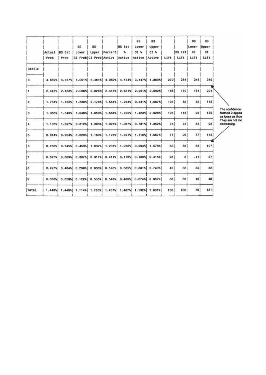
Figure

6.12

Bootstrap

confidence

interval

gains

table— Method

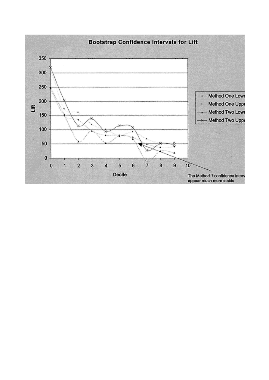
Figure

6.13

Bootstrap

confidence

interval

model

comparison

graph.

inc_est2 tot_bal2 tot_acc2 amtpdue sgle_ind
table val_dec=' ' all='Total',
infd_ag2='Infrd Age'*mean=' '*f=6.1
inc_est3='Est Income (000)'*mean=' '*f=dollar6.1
amtpdue='Amount Past Due'*mean=' '*f=dollar6.1
credlin2='Average Credit Line'*mean=' '*f=dollar10.1
tot_bal2='Average Total Balance'*mean=' '*f=dollar10.1
tot_acc2='Average Total Accounts'*mean=' '*f=9.1
mortin1n='% 1st Mort'*pctsum>val_dec all>=' '*f=7.2
mortin2n='% 2nd Mort'*pctsum<val_dec all>=' '*f=7.2
sgle_ind='% Single'*pctsum<val_dec all>=' '*f=7.2
gender_d='% Male'*pctsum<val_dec all>=' '*f=7.2
apt_indn='% in Apart -ment'*pctsum<val_dec all>=' '*f=7.2
/rts = 10 row=float box=' Decile';
run;

The resulting gains table in Figure 6.14 displays the trends for key variables across deciles. Inferred age is displayed as an average
value per decile. It is clear that the younger prospects have a higher likelihood of becoming active. Financial trends can be seen in
the next four columns. The remaining variables show the percentages of a given condition. For first mortgage indicator, the percent
with a first mortgage is higher in the lower deciles. This is also true for the second mortgage indicator. The final three columns
show the percentage of males, singles, and apartment dwellers. Each of these characteristics is positively correlated with response.
By creating this type of table with key model

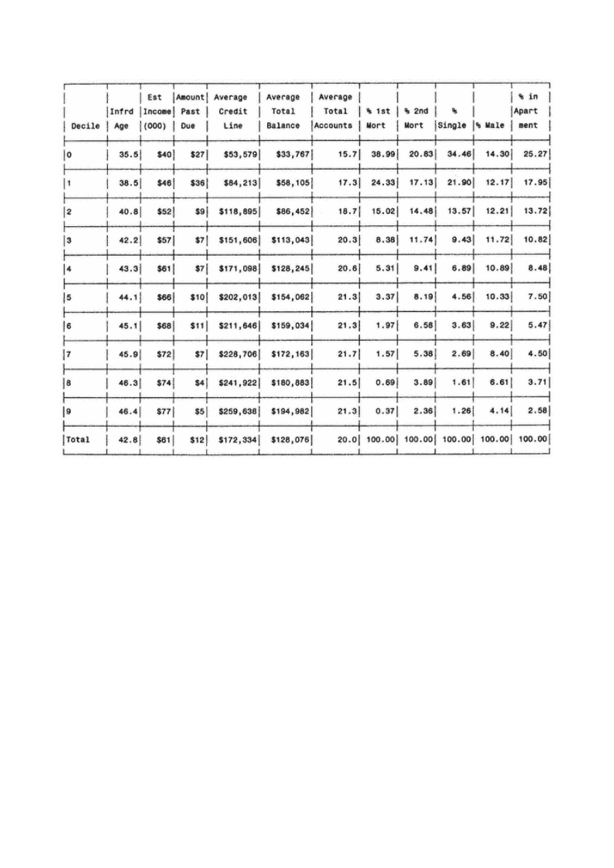
Page 149

Figure

6.14

Key

variable

validation

gains

table.

Page 150

drivers, you can verify that the prospects in the best deciles resemble your typical best prospects.

Summary

In this chapter, we learned some common -sense methods for validating a model. The reason for their success is simple.
Rather than explain a relationship, the models assign probabilities and rank prospects, customers, or any other group on
their likelihood of taking a specific action. The best validation techniques simply attempt to simulate the rigors of actual
implementation through the use of alternate data sets, resampling, and variable decile analysis. Through these methods,
we've concluded that Method 1 produced a more stable model. Now that we're satisfied with the finished product, let's
explore ways to put the models in practice.

Team-Fly

Page 151

Chapter 7—
Implementing and Maintaining the
Model

Our masterpiece survived the taste tests! Now we must make sure it is served in style.

Even though I have worked diligently to create the best possible model, the results can be disastrous if the model is not
implemented correctly. In this chapter, I discuss the steps for automated and manual scoring, including auditing
techniques. Next, I describe a variety of name selection scenarios that are geared toward specific goals like maximizing
profits, optimizing marketing efficiency or capturing market share. And finally, I describe some methods for model
tracking and troubleshooting. These are all designed to keep your data kitchen in good order!

Scoring a New File

A model is generally designed to score a new data set with the goal of improving the name selection for a new
campaign. This is typically done in one of two ways: The data set is brought in-house to be scored, or the scoring
algorithm is sent out for scoring by the data vendor or service bureau. In either case, you need to ensure that the data
being scored is similar to the data on which the model was developed by performing prescoring validation. If the new
data is from the same source as the model development data, the characteristics

Page 152

should be very similar. If the new names are from a different source, it may be necessary to factor in those differences
when projecting the model performance. They both, however, warrant scrutiny to ensure the best results.

Scoring In-house

As I demonstrated in chapter 6, the PROC LOGISTIC technique in SAS provides an option that creates a data set
containing the coefficients and other critical information for scoring a new data set. Using PROC SCORE, it simply
matches the file containing the scoring algorithm to the file needing to be scored. This can be done only after the new
data set is read into SAS and processed to create the final variables to be scored.

Data Validation

Recall how I scored data from an alternate state using the one-step model developed in our case study. Because the data
was from the same campaign, I knew the variables were created from the same source. We therefore knew that any
differences in characteristics were due to geography.

Similarly, a model implemented on data from the same source as the model development data should have similar
characteristics and produce similar scores. These differences are quantified using descriptive statistics, as shown in the
alternate state case in chapter 6. Although it is not usually the intention, it is not uncommon for a model to be developed
on data from one source and to be used to score data from another source. In either case, key drivers can be identified
and quantified to manage model performance expectations:

Population or market changes. These are the most common causes of shifting characteristic values and scores. These
changes affect all types and sources of data. The fast-growing industries are most vulnerable due to rapid market
changes. This has been apparent in the credit card industry over the last 10 years, with huge shifts in average debt and
risk profiles. Newer competitive industries like telecom and utilities will experience rapid shifts in market characteristics
and behavior.

Different selection criteria. As I discussed in chapter 2, model development data typically is extracted from a prior
campaign. The selection criteria for this prior campaign may or may not have been designed for future model
development. In either case, there is often a set of selection criteria that is business-based. In other words, certain rules,
perhaps unrelated to the goal of the model, are used for name selection and extraction. For example, a life insurance
product may not be approved for someone under age 18. Or a certain product may be appropriate only for adults with
children. Banks often have rules about not offering loan products to anyone

Page 153

who has a bankruptcy on his or her credit report. In each of these cases, certain groups would be excluded from the
file and by default be ineligible for model development. Therefore, it is important to either match the selection
criteria in scoring or account for the differences.

Variation in data creation. This is an issue only when scoring data from a different source than that of the model
development data. For example, let's say a model is developed using one list source, and the main characteristics used in
the model are age and gender. You might think that another file with the same characteristics and selection criteria
would produce similar scores, but this is often not the case because the way the characteristic values are gathered may
vary greatly. Let's look at age. It can be self-reported. You can just imagine the bias that might come from that. Or it can
be taken from motor vehicle records, which are pretty accurate sources. But it's not available in all states. Age is also
estimated using other age -sensitive characteristics such as graduation year or age of credit bureau file. These estimates
make certain assumptions that may or may not be accurate. Finally, many sources provide data cleansing. The missing
value substitution methodology alone can create great variation in the values.

Market or Population Changes

Now we've seen some ways in which changes can occur in data. In chapter 6, I scored data from an alternate state and
saw a considerable degradation in the model performance. A simple way to determine what is causing the difference is
to do some exploratory data analysis on the model variables. We will look at a numeric form of the base values rather
than the transformed values to see where the differences lie. The base variables in the model are home equity
(hom_equ), inferred age (infd_age ), credit line (credlin), estimated income (inc_est), first mortgage indicator (mortin1n),
second mortgage indicator (mortin2n), total open credit accounts (totopac), total credit accounts (tot_acc), total credit
balances (tot_bal), population density (popdensbc), apartment indicator (apt_indd ), single indicator (sgle_ind), gender
(gender_d ), child indicator, (childind), occupational group (occu_g), number of 90-day delinquencies (no90de_e ), and
accounts open in the last six months (actopl6d ). (For some categorical variables, I analyze the binary form that went into
the model.) The following code creates a comparative nonweighted means for the New York campaign (the data on
which the model was developed) and the more recent Colorado campaign:

proc means data=acqmod.model2 maxdec=2;
VAR INFD_AG CREDLIN HOM_EQU INC_EST MORTIN1N MORTIN2N TOTOPAC TOT_ACC
TOT_BAL POPDNSBC APT_INDD SGLE_IND GENDER_D CHILDIND OCC_G NO90DE_D
ACTOPL6D;
run;

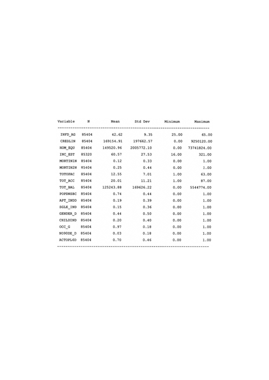
Page 154

proc means data=acqmod.colorad2 maxdec=2;
VAR INFD_AG CREDLIN HOM_EQU INC_EST MORTIN1N MORTIN2N TOTOPAC TOT_ACC
TOT_BAL POPDNSBC APT_INDD SGLE_IND GENDER_D CHILDIND OCC_G NO90DE_D
ACTOPL6D;
run;

In Figures 7.1 and 7.2, we compare the values for each variable. We see that there are some large variations in mean
values and maximum values. The average credit line is almost 50% higher in New York. The home equity values are
over 300% higher for New York. And total credit balances are twice as high in New York. These differences would
account for the differences in the model scores.

Different Selection Criteria

To determine if name selects have been done properly, it would be necessary to look at a similar analysis and check
ranges. For example, if we knew that the name selects for Colorado should have been between 25 and 65, it is easy to
check this on the means analysis.

Figure

7.1

Means

analysis

model

variables

for

New

York.

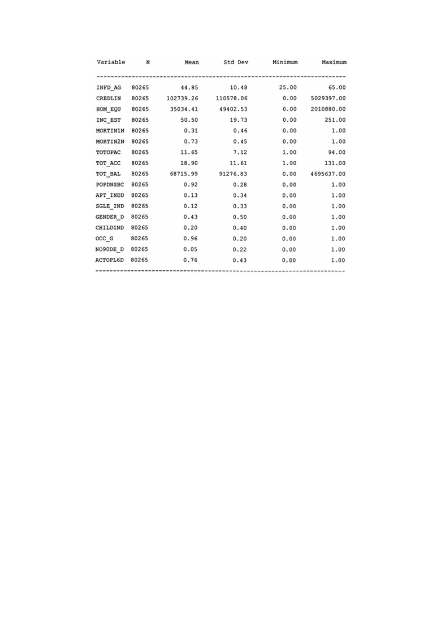
Page 155

Figure

7.2

Means

analysis

model

variables

for

Colorado.

Variation in Data Sources

This is the toughest type of discrepancy to uncover. It requires researching the source of each variable or characteristic
and understanding how it is created. If you are combining data from many sources on an ongoing basis, doing this
research is worthwhile. You need to make sure the measurements are consistent. For example, let's say the variable,
presence of children, turns out to be predictive from one data source. When you get the same variable from another data
source, though, it has no predictive power. If may be a function of how that variable was derived. One source may use
census data, and another source may use files from a publishing house that sells children's magazines. There will always
be some variations from different sources. The key is to know how much and plan accordingly.

Outside Scoring and Auditing

It is often the case that a model is developed in-house and sent to the data vendor or service bureau for scoring. This
requires that the data processing code (including all the variable transformations) be processed off-site. In this

Page 156

situation, it is advisable to get some distribution analysis from the data provider. This will give you an idea of how well
the data fits the model. In some cases, the data processing and scoring algorithm may have to be translated into a
different language. This is when a score audit is essential.

A score audit is a simple exercise to validate that the scores have been applied correctly. Let's say that I am sending the
data processing code and scoring algorithm to a service bureau. And I know that once it gets there it is translated into
another language to run on a mainframe. Our goal is to make sure the coding translation has been done correctly. First I
rewrite the code so that it does not contain any extraneous information. The following code highlights what I send:

******* CAPPING OUTLIERS ******;
%macro cap(var, svar);
proc univariate data=acqmod.audit noprint;
var &var;
output out=&svar.data std=&svar.std pctlpts= 99 pctlpre=&svar;
run;

data acqmod.audit;
set acqmod.audit;
if (_n_ eq 1) then set &svar.data(keep= &svar.std &svar.99);
if &svar.std > 2*&svar.99 then &var.2 = min(&var,(4*&svar.99)); else
&var.2 = &var;
run;

%mend;
%cap(infd_ag, age)
%cap(tot_acc, toa)
%cap(hom_equ, hom)
%cap(actop16, acp)
%cap(tot_bal, tob)
%cap(inql6m, inq)
%cap(totopac, top)
%cap(credlin, crl)
%cap(age_fil, aof)

This capping rule works only for variables with nonnegative values. With a slight adjustment, it can work for all values.
Also, please note that as a result of the capping macro, each continuous variable has a '2' at the end of the variable name.

********* DATES *********;
data acqmod.audit;
set acqmod.audit;
opd_bcd3 = mdy(substr(opd_bcd2,5,2),'01',substr(opd_bcd2,1,4));
fix_dat = mdy('12','01','1999');

Page 157

if opd_bcd3 => '190000' then
bal_rat = tot_bal2/((fix_dat - opd_bcd3)/30);
else bal_rat = 0;
run;

The following code creates the variable transformations for inferred age (infd_ag). This step is repeated for all
continuous variables in the model. PROC UNIVARIATE creates the decile value (age10) needed for the binary form of
age. Age_cos and age_sqi are also created. They are output into a data set called acqmod.agedset;

************* INFERRED AGE *************;

data acqmod.agedset;
set acqmod.audit(keep=pros_id infd_ag2);
age_cos = cos(infd_ag2);
age_sqi = 1/max(.0001,infd_ag2**2);
run;

Now I sort each data set containing each continuous variable and its transformations.

%macro srt(svar);
proc sort data = acqmod.&svar.dset;
by pros_id;
run;
%mend;
%srt(age)
%srt(inc)
%srt(hom)
%srt(toa)
%srt(tob)
%srt(inq)
%srt(top)
%srt(crl)
%srt(brt)

proc sort data = acqmod.audit;
by pros_id;
run;

Finally, I merge each data set containing the transformations back together with the original data set (acqmod.audit) to
create acqmod.audit2:

data acqmod.audit2;
merge
acqmod.audit
acqmod.agedset(keep = pros_id age_cos age_sqi)
acqmod.incdset(keep = pros_id inc_sqrt)
acqmod.homdset(keep = pros_id hom_cui hom_med)

Page 158

acqmod.toadset(keep = pros_id toa_tan toa_cu)
acqmod.tobdset(keep = pros_id tob_log)
acqmod.inqdset(keep = pros_id inq_sqrt)
acqmod.topdset(keep = pros_id top_logi top_cu top_cui)
acqmod.crldset(keep = pros_id crl_low)
acqmod.brtdset(keep = pros_id brt_med brt_log);
by pros_id;
run;

The final portion of the code is the scoring algorithm that calculates the predicted values (pres_scr). It begins by
calculating the sum of the estimates (sum_est). It is then put into the logistic equation to calculate the probability:

data acqmod.audit2;
set acqmod.audit2;
estimate = -7.65976
- 0.000034026 * hom_cui
- 0.18209 * age_cos
+ 372.299 * age_sqi
- 0.20938 * inc_sqrt
+ 0.32729 * mortal1
+ 0.62568 * mortal3
+ 0.30335 * hom_med
+ 0.0023379 * toa_tan
+ 0.0000096308 * toa_cu
+ 0.040987 * tob_log
+ 0.11823 * inq_sqrt
+ 0.00031204 * top_logi
- 0.000024588 * top_cu
- 3.41194 * top_cui
+ 0.63959 * crl_low
+ 0.14747 * brt_log
- 0.30808 * brt_med
- 0.25937 * popdnsbc
+ 0.13769 * apt_indd
+ 0.4890 * sgle_ind
+ 0.39401 * gender_d
- 0.47305 * childind
+ 0.60437 * occ_g
+ 0.68165 * no90de_d
- 0.16514 * actopl6d;
pred_scr = exp(estimate)/(1+exp(estimate));
smp_wgt = 1;
run;

Once the service bureau has scored the file, your task is to make sure it was scored correctly. The first step is to request
from the service bureau a random sample of the scored names along with the scores they calculated and all of the
necessary attributes or variable values. I usually request about 5,000 records. This allows for some analysis of expected
performance. It is important to get a

Page 159

random sample instead of the first 5,000 records. There is usually some order in the way a file is arranged, so a random
sample removes the chance of any bias.

Once the file arrives, the first task is to read the file and calculate your own scores. Then for each record you must
compare the score that you calculate to the score that the service bureau sent you. The following code reads in the data:

libname acqmod 'c:\insur\acquisit\modeldata';

data acqmod.test;
infile 'F:\insur\acquisit\audit.txt' missover recl=72;
input
pop_den $ 1 /*population density*/
apt_ind $ 2 /*apartment indicator*/
inc_est 3 -6 /*estimated income in dollars*/
sngl_in $ 7 /*marital status = single*/
opd_bcd $ 8 -13 /*bankcard open date*/
occu_cd $ 14 /*occupation code*/
gender $ 15 /*gender*/
mortin1 $ 16 /*presence of first mortgage*/
mortin2 $ 17 /*presence of second mortgage*/
infd_ag 18-19 /*inferred age*/
homeq_r $ 21 /*home equity range*/
hom_equ $ 22-29 /*home equity*/
childin $ 30 /*presence of child indicator*/
tot_acc 31-33 /*total credit accounts*/
actopl6 34-36 /*# accts open in last 6 mos*/
credlin 37-43 /*total credit lines*/
tot_bal 44-50 /*total credit card balances*/
inql6mo 51-53 /*# credit inquiry last 6 months*/
age_fil 54-56 /*age of file*/
totopac 57-59 /*total open credit accounts*/
no90eve 60-62 /*number 90 day late ever*/
sumbetas 63-67 /*sum of betas*/
score 68-72 /*predicted value*/
;
run;

The code to create the variable transformations and score the file is identical to the previous code and won't be repeated
here. One additional variable is created that compares the difference in scores (error). Once I have read in the data and
scored the new file, I test the accuracy using proc means:

data acqmod.test;
set acqmod.test;
estimate = -7.65976
- 0.000034026 * hom_cui
| | |
| | |
- 0.16514 * actopl6d
;

Page 160

pred_scr = exp(estimate)/(1+exp(estimate));
error = score - pred_scr;
run;

proc means data = acqmod.test;
var error;
run;

Figure 7.3 shows the average amount of error or difference in the scores calculated at the service bureau and the scores
calculated in our code. Because the error is greater than .0001, I know the error is not due to rounding. A simple way to
figure out the source of the error is to create a variable that identifies those records with the large error. Then I can run a
regression and see which variables are correlated with the error.

In Figure 7.3 we see that the maximum error is .3549141. This indicates that there is a problem with the code. One
simple way to determine which variable or variables are the culprits is to run a regression with the error as the dependent
variable. The following code runs a stepwise regression with one step.

proc reg data= acqmod.test;
model error= hom_cui age_cos age_sqi inq_sqrt morta11 mortal3 hom_med
toa_tan toa_cu tob_log top_logi top_cu top_cui crl_low rat_log
brt_med popdnsbc apt_indd sgle_ind gender_d childind occ_g no90de_d
actopl6d/
selection = maxr stop=1;
run;

We see from the output in Figure 7.4 that the variable gender_d is highly correlated with the error. After a discussion
with the service bureau, I discover that the coefficient for the variable, gender_d had been coded incorrectly. This error
is corrected, another sample file is provided, and the process is repeated until

Figure

7.3

Score

comparison

error.mplementing

and

Maintaining

the

Model

Team-Fly

Page 161

Figure

7.4

Regression

error.

the maximum error rate is less than .0001. (The minimum error rate must also be greater than -.0001.)

Implementing the Model

We have done a lot of work to get to this point. Now we have an opportunity to see the financial impact of our efforts.
This stage is very rewarding because we can relate the results of our work to the bottom line. And management will
definitely notice!

Calculating the Financials

Recall that in chapter 4 I defined net present value (NPV) as the value in today's dollars of future profits for a life
insurance campaign. When averaged over a group of prospects, it might also be considered the lifetime value. However,
we are not considering future sales at this stage. That model is developed in chapter 12. So I will use the term average
net present value to differentiate it from the lifetime value model in chapter 12.

The average NPV consists of four major components: the probability of activation, the risk index, the net present value
of the product profitability, and the

Page 162

marketing expense. (These are defined in detail in chapter 4.) They are combined as follows::

Average Net Present Value = P(Activation) × Risk Index × NPV of Product Profitability – Marketing Expense

The probability of activation comes directly from our model. The risk index uses the values from Table 4.1. Table 7.1
shows how the NPV of the 3-year product profitability is derived. Gross profit is revenues minus costs. Net present
value of profits is gross profit divided by the discount rate. This is discussed in more detail in chapter 12. The sum of the
net present value over 3 years divided by the number of initial customers equals $811.30. This is called the average net
present value or lifetime value for each customer for a single product.

The first step is to assign a risk score to each prospect based on a combination of gender, marital status, and inferred age
group from Table 4.1:

data acqmod.test;
set acqmod.test;
if gender = 'M' then do;
if marital = 'M' then do;
if infd_ag2 < 40 then risk_adj = 1.09;
else if infd_ag2 < 50 then risk_adj = 1.01;
else if infd_ag2 < 60 then risk_adj = 0.89;
else risk_adj = 0.75;
end;
else if marital = 'S' then do;
if infd_ag2 < 40 then risk_adj = 1.06;
| | | | |
| | | | |
else if marital = 'W' then do;

Table 7.1

Average Net Present Value Calculation for Single Product

INITIAL SALE

1ST YEAR

RENEWAL

2ND YEAR

RENEWAL

3RD YEAR

Initial customers

50,000

35,500

28,045

Renewal rate

71%

79%

85%

Total revenue

$30,710,500

$21,804,455

$17,225,519

Policy maintenance & claims

$9,738,150

$8,004,309

$7,184,680

Gross profit

$20,972,350

$13,800,146

$10,040,839

Discount rate

1.00

1.15

1.32

Net present value

$20,972,350

$12,000,127

$7,592,317

Cumulative net present value

$20,972,350

$32,972,477

$40,564,794

Average net present value

419.45

659.45

811.30

Page 163

if infd_ag2 < 40 then risk_adj = 1.05;
else if infd_ag2 < 50 then risk_adj = 1.01;
else if infd_ag2 < 60 then risk_adj = 0.92;
else risk_adj = 0.78;
end;
end;

The next step assigns the average net present value of the product profitability, prodprof. And finally the average net
present value (npv_3yr) is derived by multiplying the probability of becoming active (pred_scr) times the risk
adjustment index (risk_adj) times the sum of the discounted profits from the initial policy (prodprof) minus the initial
marketing expense:

prodprof = 811.30;
npv_3yr= pred_scr*risk_adj*prodprof - .78;
run;
proc sort data=acqmod.test;
by descending npv_3yr;
run;

data acqmod.test;
set acqmod.test;
smp_wgt=1;
sumwgt=5000;
number+smp_wgt;
if number < .1*sumwgt then val_dec = 0; else
if number < .2*sumwgt then val_dec = 1; else
if number < .3*sumwgt then val_dec = 2; else
if number < .4*sumwgt then val_dec = 3; else
if number < .5*sumwgt then val_dec = 4; else
if number < .6*sumwgt then val_dec = 5; else
if number < .7*sumwgt then val_dec = 6; else
if number < .8*sumwgt then val_dec = 7; else
if number < .9*sumwgt then val_dec = 8; else
val_dec = 9;
run;

proc tabulate data=acqmod.test;
weight smp_wgt;
class val_dec;
var records pred_scr risk_adj npv_3yr;
table val_dec='Decile' all='Total',
records='Prospects'*sum=' '*f=comma10.
pred_scr='Predicted Probability'*(mean=' '*f=11.5)
risk_adj = 'Risk Index'*(mean=' '*f=6.2)
npv_3yr = 'Total 3-Year Net Present Value'
*(mean=' '*f=dollar8.2)
/rts = 9 row=float;
run;

Page 164

TIP

If you have a very large file and you want more choices for determining where to make a
cut-off, you can create more groups. For example, if you wanted to look at 20 groups
(sometimes called twentiles), just divide the file into 20 equal parts and display the
results.

A model is a powerful tool for ranking customers or prospects. Figure 7.5 shows the expected active rate, average risk
index, and three-year present

Figure

7.5

Decile

analysis

scored

file.

Page 165

value by decile for the new file based on the sample that was scored. The model, however, does not provide the rules for
making the final name selections. The decision about how deep to go into a file is purely a business decision.

In Figure 7.6, I plug the expected active rate for each decile into the NPV formula. The columns in the table are used to
calculate the NPV projections necessary to make an intelligent business decision:

Prospects. The number of prospects in the scored file.

Predicted active rate. The rate per decile from Figure 7.5.

Risk index. The average risk based on a matrix provided by actuarial (see Table 4.1).

Product profitability. The expected profit from the initial policy discounted in today's dollars. The values are the same
for every prospect because the model targets only one product. The calculation for discounting will be explained in
chapter 12.

Average NPV. The average three-year profit from the one product offered, discounted in today's
dollars.

Average cumulative NPV. The cumulative of average NPV.

Sum of cumulative NPV. The cumulative total dollars of NPV.

Figure

7.6

NPV

model

gains

table.

Page 166

Determining the File Cut-off

Once the file has been scored and the financials have been calculated, it's time to decide how many names to select or
how much of the file to solicit. This is typically called the file cut-off. Figure 7.6 does an excellent job of providing the
information needed for name selection. It, however, doesn't give the answer. There are a number of considerations when
trying to decide how many deciles to solicit. For example, at first glance you might decide to cut the file at the fifth
decile. The reason is rather obvious: This is last decile in which the NPV is positive. There are a number of other good
choices, however, depending on your business goals.

Let's say you're a young company going after market share. Management might decide that you are willing to spend
$0.25 to bring in a new customer. Then you can cross-sell and up-sell additional products. This is a very reasonable
approach that would allow you to solicit eight deciles. (In chapter 12, I will develop a lifetime value model that
incorporates cross-sell and up-sell potential.)

Perhaps your company decides that it must make a minimum of $0.30 on each customer to cover fixed expenses like
salaries and building costs. In this situation, you would solicit the first four deciles. Another choice could be made based
on model efficiency. If you look at the drop in NPV, the model seems to lose its high discrimination power after the
third decile.

It's important to note that any decision to cut the file at a certain dollar (or cents) amount does not have to be made using
deciles. The decile analysis can provide guidance while the actual cut -off could be at mid -decile based on a fixed
amount. In our previous example, the average for decile 4 is $0.30. But at some point within that decile, the NPV drops
below $0.30, so you might want to cut the file at an NPV of $0.30. The main point to remember is that selecting the file
cut-off is a business decision. The decile analysis can provide guidance, but the decision must be clear and aligned with
the goals of the business.

Champion versus Challenger

In many situations, a model is developed to replace an existing model. It may be that the old model is not performing. Or
perhaps some new predictive information is available that can be incorporated into a new model. Whatever the reason, it
is important to compare the new model, or the ''Challenger," to the existing model, or "Champion." Again, depending on
your goals, there are a number of ways to do this.

In Figure 7.7, we see the entire file represented by the rectangle. The ovals represent the names selected by each model.
If your "Champion" is doing well, you

Page 167

Figure

7.7

Champion

versus

Challenger.

might decide to mail the entire file selected by the "Champion" and mail a sample from the portion of the "Challenger"
oval that was not selected by the "Champion." This allows you to weight the names from the sample so you can track
and compare both models' performance.

At this point, I have calculated an expected net present value for a single product. This is an excellent tool for estimating
the long-term profitability of a customer based on the sale of a single product. We know that one of our company goals
is to leverage the customer relationship by selling additional products and services to our current customer base. As
mentioned previously, in chapter 12 I expand our case study to the level of long-term customer profitability by
considering the present value of future potential sales. I will integrate that into our prospect model to calculate lifetime
value.

The Two-Model Matrix

I decided against using the two -model approach because of instability. However, it may be preferred in certain situations
because of its flexibility. Because the models have been built separately, it is possible to manage the components
separately. This may be very useful for certain business strategies. It can also make the model performance easier to
track. In other words, you can monitor response and activation separately.

The code is similar to the one -model code. The difference is that the decile values have to be calculated and blended
together. The first step is to sort the

Page 168

validation data by the response score (predrsp ), create deciles called rsp_dec, and output a new data set. The steps are
repeated to create deciles in a new data set based on activation called act_dec.

proc sort data=acqmod.out_rsp2(rename=(pred=predrsp));
by descending predrsp;
run;

proc univariate data=acqmod.out_rsp2(where=( splitwgt = .)) noprint;
weight smp_wgt;
var predrsp;
output out=preddata sumwgt=sumwgt;
run;

data acqmod.validrsp;
set acqmod.out_rsp2(where=( splitwgt = .));
if (_n_ eq 1) then set preddata;
retain sumwgt;
number+smp_wgt;
if number < .1*sumwgt then rsp_dec = 0; else
if number < .2*sumwgt then rsp_dec = 1; else
if number < .3*sumwgt then rsp_dec = 2; else
if number < .4*sumwgt then rsp_dec = 3; else
if number < .5*sumwgt then rsp_dec = 4; else
if number < .6*sumwgt then rsp_dec = 5; else
if number < .7*sumwgt then rsp_dec = 6; else
if number < .8*sumwgt then rsp_dec = 7; else
if number < .9*sumwgt then rsp_dec = 8; else
rsp_dec = 9;
run;

proc sort data=acqmod.out_act2(rename=(pred=predact));
by descending predact;
run;

proc univariate data=acqmod.out_act2(where=(splitwgt = .)) noprint;
weight smp_wgt;
var predact active;
output out=preddata sumwgt=sumwgt;
run;

data acqmod.validact;
set acqmod.out_act2(where=( splitwgt = .));
if (_n_ eq 1) then set preddata;
retain sumwgt;
number+smp_wgt;
if number < .1*sumwgt then act_dec = 0; else
if number < .2*sumwgt then act_dec = 1; else

Page 169

if number < .3*sumwgt then act_dec = 2; else
if number < .4*sumwgt then act_dec = 3; else
if number < .5*sumwgt then act_dec = 4; else
if number < .6*sumwgt then act_dec = 5; else
if number < .7*sumwgt then act_dec = 6; else
if number < .8*sumwgt then act_dec = 7; else
if number < .9*sumwgt then act_dec = 8; else
act_dec = 9;
activ_r = 0; activ_r = activate;
run;

Next, the two data sets are sorted and merged by pros_id. PROC TABULATE is used create a cross-matrix of values.

proc sort data=acqmod.validrsp;
by pros_id;
run;

proc sort data=acqmod.validact;
by pros_id;
run;

data acqmod.blend;
merge acqmod.validrsp acqmod.validact;
by pros_id;
run;

proc tabulate data=acqmod.blend;
weight smp_wgt;
class rsp_dec act_dec;
var respond active records activ_r;
table (rsp_dec='Response Decile' all='Total')*
(records='Count'*sum=' '*f=comma7.
activ_r='Actv Rate'*(mean=' '*f=percent5.2)
respond='Resp Rate'*(mean=' '*f=percent5.2)),
(act_dec='Active Decile' all='Total') /rts = 21 row=float;
run;

The resulting table is very busy and uninteresting, but the values are transferred to a spreadsheet and graph. In Figure
7.8, we see a three-dimensional graph that shows the frequency of each response decile crossed with each
active|response decile. This could be used to determine cut-offs that meet certain minimum response rates as well as
minimum approval rates. As mentioned previously, it is also useful if you want to track model performance separately.
For example, the response model could stop performing while the approval model continues to do well. In this case, you
would have to rebuild only the response model.

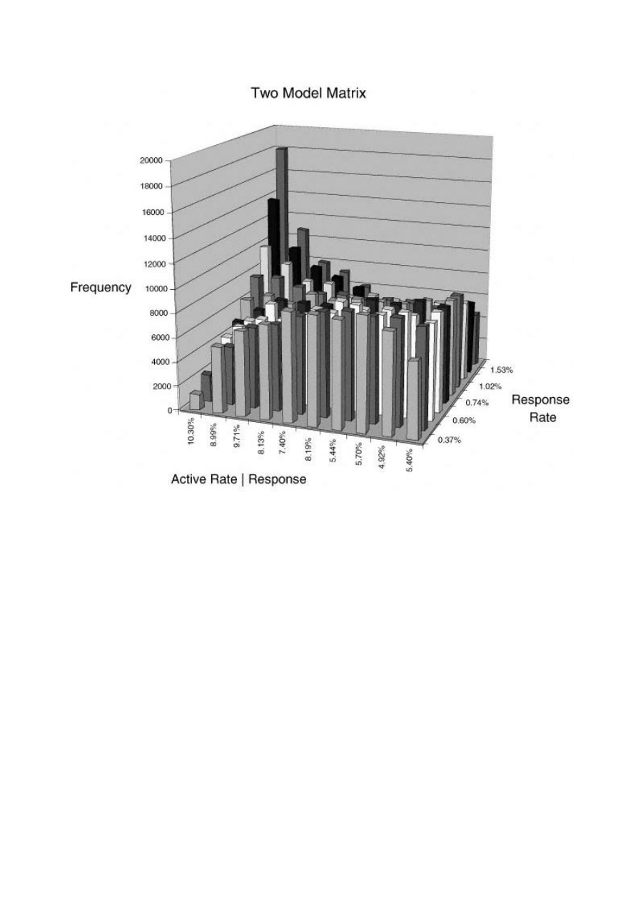
Page 170

Figure

7.8

Two

Model

Approach.

Model Tracking

Throughout this book, I have stressed that the steps surrounding model development are key to the success of a model.
At this point, if things don't go as expected it may be necessary to figure out what went wrong. In the accompanying
sidebar, Allison Cornia presents her top 10 list for sleuthing out the problem.

When Good Models Go Bad

Allison Cornia, Vice President at Microsoft Corporation, discusses her top 10 list of techniques for tracking
problems in models.

Building a good model isn't just about sound analytic work. A good targeted-marketing campaign is like a
precisely engineered motor. Every part of the process depends on another for success. And every once in a
while, a target-marketing campaign doesn't work as planned. "Response wasn't very high." "The cus-

Team-Fly

Page 171

tomers didn't materialize." "Sales barely even moved enough for a rounding error." Knowing that
something is not working is easy. Figuring out where the campaign went wrong is the difficult part. As a
modeler, you may be surprised at what happens to your work when you are finished. With so many steps to
the process, how do you know where things went wrong? What do you do when you have a proven offer
and creative but the campaign flops? The following list is my top 10 troubleshooting tips when it appears
that your arrow has not hit its target.

1. Check the phones. This sounds really obvious, but if the phones aren't ringing within days (for direct
mail) or minutes (for e -mail and direct TV) after the offer has hit, check your inbound call system. I had one
customer call me and say, "The phones aren't ringing. The models (the data) are bad!" I furiously checked
the data processing and reviewed the analytical procedures looking for why response was so far off. Later I
learned that the Vice President of Marketing for the marketing company was terminated for a faulty phone
system.

It seems really elementary. But the stories abound where the phone number was printed incorrectly or
pointed to the wrong department, or the system just plain didn't work. It is crucial to make sure the inbound
path is configured properly as well. I recently had an experience as a consumer in which, when I followed
the automated attendant's instructions, it dead-ended me every time. And as result, the company did not get
my business. So the message here is to test the system. And not just from your phone at the office, but have
people in different parts of the country call at different times prior to launch.

And in this day of dot -commerce, the same applies with a slight twist. Check the Web site. If you are sending
people to a specific URL, make sure they get there without receiving an error message. Make sure they can
click through to suggested sites, make real sure they can click on the "BUY NOW'' button, and be absolutely
sure they can complete their transaction. In these early days of e-commerce, those that give purchasers an
effortless and secure transaction experience are going to be winning now and dominating in the future.

2. Track the mail. With first-class mail, it is reasonably easy to predict delivery times. However, it is not
entirely infallible. If you have shipped mail to other parts of the country, make sure you know what day the
mail actually dropped. The USPS is beta testing a new bar code on mail that allows people to track first-class
mail much like overnight deliveries. Once this software is released and becomes more widely available, it
will be easier to judge when the calls/clicks should start arriving. I always lose sleep after a mail drop
because I know that until the phones start to ring, people are apt to get anxious and point fingers at the data.
Timing on the mail drop should also be evaluated to avoid the "dead seasons" in direct response (i.e., the
week of Christmas).

continues

Page 172

(Continued)

3. Listen in on your call center. If response seems high and/or acceptable but conversion rates are low,
listen in on customer calls. Are your customers getting through in acceptable amounts of time? Or are they
spending lots of time on hold? Is the Web site up to the traffic load, or are people unable to access the site?
Listen to the call reps. Are they courteous and helpful? Are they answering questions correctly about the
products they are selling? This can be helpful in a number of ways. First and foremost, you will be able to
tell what kind of experience your customers are having and how well that meets expectations. Second, if
there is a bad fit between the data and the creative, the call center representatives will tell you with their
comments or lack of sales. In one example from the financial services sector, a large well -known dot.com
mortgager sent out a great offer. However, it was a new product, and the target data was difficult to define
based on the product definition. While response was phenomenal, the conversion rates were low as many
responders were not qualified for the product. By talking to the call center reps, we could tell many of the
problems with the targeting, and adjustments could be made before the next wave of mail went out.

4. Check the implementation of the model/targeting. Whether you are using an algorithm or a
segmentation schema, make sure that the "scoring" or implementation has gone correctly. Most people will
perform a validation of the coding on a small sample that is usually held out from the modeling process. In
today's environment of "big data," it is difficult and sometimes impossible to validate scores on entire
databases. Most of the time, the culprit is not an error in the coding or scoring but the underlying data in the
database. Because of the size of most data marts, not every field may have been "vetted" properly. While the
sample may have had "clean" data in it, the database to which you are applying it may have values that are
widely skewed, corrupt, dirty, or not there at all. One way to counteract this is to take several samples from
the database and apply the scores/schema. Look at the underlying data. Does it mirror what you would
expect to find? If you are lucky enough to be able to vet your entire database, do it. Anything other than
being able to validate in the entire environment pales in comparison.

5. Was the right group pulled? Again, this might seem elementary but I have seen many examples where
the model/schema was applied properly, but the data extracted for the fulfillment house was incorrect. Make
sure that your programmers understand that "1'' is the top decile and "10" is really not the group you are
after. Most of us in the industry have heard horror stories about score reversals. A direct marketing agency
had to credit its customer a half million dollars in mailings because a programmer inverted a decile score.

Page 173

How can you tell this has happened to you? If response rates seem extremely low but still have somewhat
of a pulse, and if the offer is a proven offer, this may be an area that you want to investigate further. How
can you confirm it? First, take the mail file and have this group's data (that would have been used to score
them) appended. Score the model or apply the schema. Are they in the correct deciles/groups? If the answer
is yes, you may need to look elsewhere for the source of your problem. If the answer is no, perform one
other check. Go back to the main file/database where these persons' scores are stored. Pull out those names
that were mailed and confirm that they belong to the deciles/groups they should. This two-part validation
will answer two issues: Was the data scored properly to begin with, and was the model inverted? In the
example of the direct marketing agency, the problem lay with having two databases in two different IT
environments. The mainframe held the main database and was where the models were scored. A copy of
these scores and deciles was extracted and given to an IT group in a relational setting. The scores were
added to the relational environment and in doing so, the programmers ignored the decile codes and
redeciled with the highest scores being assigned to decile 10 instead of 1. In revalidating and investigating
all the efforts, if we had just compared the individual scores on the file in the relational setting without
comparing back to the mainframe, we would have missed the problem. The cautionary tale here is that it
can happen, so be careful not to let it.

6. Like a good farmer, check your crop rotation. This is another elementary point in database
management, but again it can be overlooked. I was once asked if "list fatigue" existed, and I believe it does
but can be avoided/minimized. One tactic is to develop some sound business rules that allow you to
systematically rotate your lists. In direct marketing, the rule of thumb is usually 90-day intervals. There are
some exceptions, though. With in-house files/databases, in-depth profiling will tell you what your frequency
should be for talking to the customer. Some customers love constant communications (frequent purchasers,
heavy users), while others would prefer you never talk to them (the opt-outs). E-mail solicitations have
become very popular, mainly due to the low costs associated with producing them, but caution should be
exercised in how often you fill up someone's inbox with offers. Even though we have all become somewhat
numb to the amount of mailbox stuffers we receive, e-mail solicitations have a slightly more invasive feel
than direct mail, similar to telemarketing calls. I often wonder how businesses that I haven't bought from get
my e-mail address. If we as direct marketers can appreciate this distinction with e-mail and refrain from
spamming our hearts out, we can probably assure ourselves that we won't be regulated in how often we can
e-mail people and preserve a low-cost alternative for talking to our customers.

continues

Page 174

(Continued)

How can you tell if list fatigue is setting in? Are response and conversion rates gradually declining in a nice
steady curve? Can you tell me the average number of times a person is mailed and with what frequency?
Do you have business rules that prevent you from over-communicating to customers? If the answers to
these questions are yes, no, and no, chances are you aren't rotating your crops enough.

7. Does your model/schema have external validity? This is a question that sometimes is forgotten. You
have great analysts who build technically perfect models. But can anyone interpret them in the context of the
business? If the answer is no, your models/schemas do not have external validity. External validity to
modeling is analogous to common sense. For example, let's take a look at a financial services model that
finds that one of the factors in a model to predict demand for a high-interest-rate mortgage is someone's
FICO score. FICO is weighted positively, which would be interpreted to mean that someone with a really
high FICO score is more likely to convert. Well, any mortgage banker in the crowd will tell you that goes
against what really happens. People with high FICO scores are people with excellent credit and therefore
would most likely not be interested in, or likely to borrow at, high interest rates. Try evaluating and
interpreting analytical work with a marketing manager's perspective. It will help you to evaluate whether
your model/schema has external validity.

8. Does your model have good internal validity? When I refer to internal validity, I am referring to the
validity of the model/schema building process itself. There are many ways to prevent a badly built
model/schema from ever seeing the light of day. One good approach is to have the model/schema building
process formalized with validation checks and reviews built into the process. Good modelers always keep a
"hold-out" sample for validating their work. Documentation at every step of the process is good so in the
case that something goes wrong, one can follow the model-building process much like a story. Not every
modeler is very thorough. Having a formalized documentation/process can help to avoid errors. Having
modelers review each other's work is also helpful. Often, I am asked to decipher whether a model is "good"
or not by just looking at the algorithm. That in itself is not enough to determine the quality of the model.
Understanding the underlying data, as well as the process by which the modeler built the algorithm, is
crucial. In one such case, the model seemed to be valid. On reviewing the data, however, I found the culprit.
The algorithm included an occupation code variable. However, when I looked at the data, this variable was
an alphanumeric code that would have had to be transformed to be of any use in a model. And that hadn't
happened. This example brings up another related issue. With the explosion in the importance and demand
for dataminers, there are many groups/people operating out there who are less than thorough when building
models/schemas. If someone builds you a model, ask him or her to detail the process by which he

Page 175

or she built it and by what standards he or she evaluated it. If you aren't sure how to evaluate his or her
work, hire or find someone who can.

9. Bad ingredients make bad models. Nothing will ruin a model or campaign faster than bad data. Model-
building software has become so automated that anyone can build a model with a point and click. But the
real service that an experienced analyst brings is being able to detect bad data early on. EDA, or exploratory
data analysis, is the first step toward building a good model/schema and avoiding the bad data experience. If
you are the analyst, don't take someone's word that the data is what it is; check it out for yourself. Know your
data inside and out. I once had an experience where the client gave me all the nonresponders but told me they
were responders. Only when I got to the part where I checked my external validity did I find the problem and
correct it. If you work in database marketing, don't assume that others understand data the same way.
Confirm how samples are pulled, confirm data content, and examine files very closely. If you are working
with appended data, make sure that the data is clean. This is more difficult because you may not be as
familiar with it. Ask for ranges of values for each field and for the mean scores/frequencies for the entire
database that the data came from. A related issue with appended data is that it should make sense with what
you are trying to predict. Financial data is a very powerful ingredient in a model/schema to predict demand
for financial services, but as a predictor for toothpaste purchase behavior, it is not. Choose your ingredients
wisely.

10. Sometimes good models, like good horses, need to be put out to pasture. Good models, built on well-
chosen data, will perform over time. But like all good things, models do have a life cycle. Because not every
market is the same and consumers tend to change over time, it almost ensures that the process of prediction
will not be an event. How can you tell if it is time to refresh/rebuild your model? Have you seen a complete
drop-off in response/conversion without a change in your creative/offer or the market at large? If yes, it's
time to rebuild. But nobody wants to wait until that happens; you would prefer to be proactive about
rebuilding models. So, that said, how do you know when it's time? The first clue is to look at the market
itself. Is it volatile and unpredictable? Or is it staid and flat? Has something changed in the marketplace
recently (i.e., legislation, new competitors, new product improvements, new usage) that has changed overall
demand? Are you communicating/distributing through new channels (i.e., the Internet)? Have you changed
the offer/creative? All of the preceding questions will help you to determine how often and when new
models should be built. If you are proactive by watching the market, the customers, and the campaigns you
will know when it is time. One suggestion is to always be testing a "challenger" to the "established champ."
When the challenger starts to out-perform the champ consistently, it's time to retire the champ.

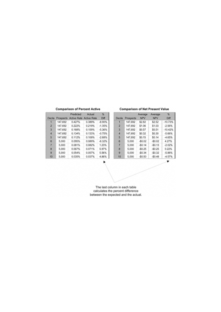
Page 176

Back-end Validation

In my opinion, the most exciting and stressful part of the modeling process is waiting for the results to come in. I usually
set up a daily monitoring program to track the results. That approach can be dangerous, though, because you can't
determine the true performance until you have a decent sample size. My advice is to set up a tracking program and then
be patient. Wait until you have at least a couple hundred responders before you celebrate.

In the case study, I am predicting the probability of a prospect becoming an active account. This presumes that the
prospect responds. I can multiply the number of early responders times the expected active rate, given response, to get a
rough idea of how the campaign is performing.

Once all of the results are in, it is critical to document the campaign performance. It is good to have a standard report.
This becomes part of a model log (described in the next section). For the case study, the company mailed deciles 1
through 5 and sampled deciles 6 through 10. In Figure 7.9, the model results are compared with the expected
performance shown in Figure 7.6. Each component within each decile is compared.

We notice a slight difference in the expected performance and the actual performance. But overall, model performance is
good. For both the "active rate"

Figure

7.9

Back-end

validation

report.

Page 177

and the "average NPV," the rank ordering is strong and the variation from expected performance is at or below 10%.

Model Maintenance

I have worked with modelers, marketers, and managers for many years. And I am always amazed at how little is known
about what models exist within the corporation, how they were built, and how they have been used to date. After all the
time and effort spent developing and validating a model, it is worth the extra effort to document and track the model's
origin and utilization. The first step is to determine the expected life of the model.

Model Life

The life of a model depends on a couple of factors. One of the main factors is the target. If you are modeling response, it
is possible to redevelop the model within a few months. If the target is risk, it is difficult to know how the model
performs for a couple of years. If the model has an expected life of several years, it is always possible to track the
performance along the way.

Benchmarking

As in our case study, most predictive models are developed on data with performance appended. If the performance
window is three years, it should contain all the activity for the three-year period. In other words, let's say you want to
predict bankruptcy over a three -year period. You would take all names that are current for time T. The performance is
then measured in the time period between T + 6 to T + 36 months. So when the model is implemented on a new file, the
performance can be measured or benchmarked at each six-month period.

If the model is not performing as expected, then the choice has to be made whether to continue use, rebuild, or refresh.

Rebuild or Refresh?

When a model begins to degrade, the decision must be made to rebuild or refresh the model. To rebuild means to start
from scratch, as I did in chapter 3. I would use new data, build new variables, and rework the entire process. To refresh
means that you keep the current variables and rerun the model on new data.

Page 178

It usually makes sense to refresh the model unless there is an opportunity to introduce new predictive information. For
example, if a new data source becomes available it might make sense to incorporate that information into a new model.
If a model is very old, it is often advisable to test building a new one. And finally, if there are strong shifts in the
marketplace, a full -scale model redevelopment may be warranted. This happened in the credit card industry when low
introductory rates were launched. The key drivers for response and balance transfers were changing with the drop in
rates.

Model Log

A model log is a register that contains information about each model such as development details, key features, and an
implementation log. Table 7.2 is an example of a model log for our case study.

A model log saves hours of time and effort as it serves as a quick reference for managers, marketers, and analysts to see
what's available, how models were

Table 7.2

Sample Model Log

NAME OF MODEL

LIFEA2000

Dates of development

3/00–4/00

Model developer

O. Parr Rud

Overall objective

Increase NPV

Specific target

Accounts with premium amount > 0

Model development data (date)

NewLife600 (6/99)

First campaign implementation

NewLife750 (6/00)

Implementation date

6/15/00

Score distribution (validation)

Mean = .037, St Dev = .00059, Min = .00001,
Max = .683

Score distribution (implementation)

Mean = .034, St Dev = .00085, Min = .00001,
Max =.462

Selection criteria

Decile 5

Selection business logic

> $.05 NPV

Preselects

Age 25–65; minimum risk screening

Expected performance

$726M NPV

Actual performance

$703M NPV

Model details

Sampled lower deciles for model validation and redevelopment

Key drivers

Population density, life stage variables

Page 179

developed, who's the target audience, and more. It tracks models over the long term with details such as the following:

Model name or number. Select a name that reflects the objective or product. Combining it with a number allows for
tracking redevelopment models.

Date of model development. Range of development time.

Model developer. Name of person who developed model.

Model development data. Campaign used for model development.

Overall objective. Reason for model development.

Specific target. Specific group of interest or value estimated.

Development data. Campaign used for development.

Initial campaign. Initial implementation campaign.

Implementation date. First use date.

Score distribution (validation). Mean, standard deviation, minimum and maximum values of score on validation
sample.

Score distribution (implementation). Mean, standard deviation, minimum and maximum values of score on
implementation sample.

Selection criteria. Score cut-off or depth of file.

Selection business logic. Reason for selection criteria.

Preselects. Cuts prior to scoring.

Expected performance. Expected rate of target variable; response, approval, active, etc.

Actual performance. Actual rate of target variable; response, approval, active, etc.

Model details. Characteristics about the model development that might be unique or unusual.

Key drivers. Key predictors in the model.

I recommend a spreadsheet with separate pages for each model. One page might look something like the page in Table
7.2. A new page should be added each time a model is used. This should include the target population, date of score,
date of mailing, score distribution parameters, preselects, cut-off score, product code or codes, and results.

Summary

In this chapter, I estimated the financial impact of the model by calculating net present value. This allowed me to assess
the model's impact on the company's

Page 180

bottom line. Using decile analysis, the marketers and managers are able to select the number of names to solicit to best
meet their business goals.

As with any great meal, there is also the clean-up! In our case, tracking results and recording model development are
critical to the long-term efficiency of using targeting models.

Team-Fly

Page 181

PART THREE —
RECIPES FOR EVERY OCCASION

Page 182

Do you like holiday dinners? Are you a vegetarian? Do you have special dietary restrictions? When deciding what to
cook, you have many choices!

Targeting models also serve a variety of marketing tastes. Determining who will respond, who is low risk, who will be
active, loyal, and above all, profitable—

these are all activities for which segmentation and targeting can be valuable. In

this part of the book, I cover a variety of modeling objectives for several industries. In chapter 8, I begin with profiling
and segmentation, a prudent first step in any customer analysis project. I provide examples for both the catalog and
financial services industry using both data -driven and market-driven techniques. In chapter 9 I detail the steps for
developing a response model for a business -to -business application. In chapter 10 I develop a risk model for the
telecommunication industry. And in chapter 11, I develop a churn or attrition model for the credit card industry. Chapter
12 continues the case study from chapters 3 through 7 with the development of a lifetime value model for the direct-mail
life insurance industry.

If your work schedule is anything like mine, you must eat fast food once in a while. Well, that's how I like to describe
modeling on the Web. It's designed to handle large amounts of data very quickly and can't really be done by hand. In
chapter 13, I discuss how the Web is changing the world of marketing. With the help of some contributions from leading
thinkers in the field, I discuss how modeling, both traditional and interactive, can be used on a Web site for marketing,
risk, and customer relationship management.

Page 183

Chapter 8—
Understanding Your Customer:
Profiling and Segmentation

The methodologies discussed in this chapter could have easily been included at the beginning of this book, but because
they don't really fit into the realm of predictive modeling, I decided to write a separate chapter. The cases in this chapter
describe several techniques and applications for understanding your customer. Common sense tells us that it's a good
first step to successful customer relationship management. It is also an important step for effective prospecting. In other
words, once you know what customer attributes and behaviors are currently driving your profitability, you can use these
to direct your prospecting efforts as well. (In fact, when I decided on a title for this chapter, I was hesitant to limit it to
just ''customer.") The first step in effective prospecting is learning how to find prospects that look like your customers. It
is also useful to segment and profile your prospect base to assist acquisition efforts. The goal in both cases is to identify
what drives customer profitability.

This chapter begins by defining profiling and segmentation and discussing some of the types and uses of these
techniques. Some typical applications are discussed with references to the data types mentioned in chapter 2. The second
half of the chapter details the process using three case studies. The first is from the catalog industry, in which I perform
some simple profile and penetration analyses. Next, I develop a customer value matrix for a credit card customer
database. The final case study illustrates the use of cluster analysis to discover segments.

Page 184

What is the importance of understanding your customer?

This sounds like a dumb question, doesn't it? You would be amazed, though, at how many companies operate for
years— pumping out offers for products and services— without a clue of what their best customer looks like. For every
company in every industry, this is the most important first step to profitable marketing.

Similar to modeling, before you begin any profiling or segmentation project, it is important to establish your objective.
This is crucial because it will affect the way you approach the task. The objective can be explained by reviewing the
definitions of profiling and segmentation.

Profiling is exactly what it implies: the act of using data to describe or profile a group of customers or prospects. It can
be performed on an entire database or distinct sections of the database. The distinct sections are known as segments.
Typically they are mutually exclusive, which means no one can be a member of more than one segment.

Segmentation is the act of splitting a database into distinct sections or segments. There are two basic approaches to
segmentation: market driven and data driven. Market-driven approaches allow you to use characteristics that you
determine to be important drivers of your business. In other words, you preselect the characteristics that define the
segments. This is why defining your objective is so critical. The ultimate plans for using the segments will determine the
best method for creating them. On the other hand, data-driven approaches use techniques such as cluster analysis or
factor analysis to find homogenous groups. This might be useful if you are working with data about which you have
little knowledge.

Types of Profiling and Segmentation

If you've never done any segmentation or modeling, your customer base may seem like a big blob that behaves a certain
way, depending on the latest stimulus. If you do a little digging, you will find a variety of demographic and
psychographic characteristics as well as a multitude of buying behaviors, risk patterns, and levels of profitability among
the members of your database. This is the beauty of segmentation and profiling. Once you understand the distinct groups
within the database, you can use this knowledge for product development, customer service customization, media and
channel selection, and targeting selection.

Page 185

RFM:
Recency, Frequency, Monetary Value

One of the most common types of profiling originated in the catalog industry. Commonly called RFM, it is a method of
segmenting customers on their buying behavior. Its use is primarily for improving the efficiency of marketing efforts to
existing customers. It is a very powerful tool that involves little more than creating segments from the three groups.

Recency. This value is the number of months since the last purchase. It is typically the most powerful of the three
characteristics for predicting response to a subsequent offer. This seems quite logical. It says that if you've recently
purchased something from a company, you are more likely to make another purchase than someone who did not recently
make a purchase.

Frequency. This value is the number of purchases. It can be the total of purchases within a specific time frame or
include all purchases. This characteristic is second to recency in predictive power for response. Again, it is quite
intuitive as to why it relates to future purchases.

Monetary value. This value is the total dollar amount. Similar to frequency, it can be within a specific time frame or
include all purchases. Of the three, this characteristic is the least powerful when it comes to predicting response. But
when used in combination, it can add another dimension of understanding.

These three characteristics can be used alone or in combination with other characteristics to assist in CRM efforts.
Arthur M. Hughes, in his book Strategic Database Marketing (Probus, 1994), describes a number of excellent
applications for RFM analysis. In the second half of the chapter, I will work through a case study in which I calculate
RFM for a catalog company.

Demographic

Have you ever seen the ad that shows a 60's flower child living in a conservative neighborhood? The emphasis is on
finding the individual who may not fit the local demographic profile. In reality, though, many people who live in the
same area behave in a similar fashion.

As I mentioned in chapter 2, there are many sources of demographic data. Many sources are collected at the individual
level with enhancements from the demographics of the surrounding geographic area. Segmenting by values such as age,
gender, income, and marital status can assist in product development, creative design, and targeting.

There are several methods for using demographics to segment your database and/or build customer profiles. Later on in
the chapter, I will create a customer

Page 186

value matrix using a combination of demographic and performance measures for a database of credit card customers.

Life Stage

Whether we like it or not, we are all aging! And with few exceptions, our lives follow patterns that change over time to
meet our needs. These patterns are clustered into groups defined by demographics like age, gender, marital status, and
presence of children to form life stage segments.

Life stage segments are typically broken into young singles; couples or families; middle-aged singles, couples, or
families; and older singles or couples. Additional enhancements can be achieved by overlaying financial, behavioral, and
psychographic data to create well-defined homogeneous segments. Understanding these segments provides opportunities
for businesses to develop relevant products and fine -tune their marketing strategies.

At this point, I've spent quite a bit of time explaining and stressing the importance of profiling and segmentation. You
can see that the methodologies vary depending on the application. Before I get into our case studies, it is worthwhile to
stress the importance of setting an objective and developing a plan. See the accompanying sidebar for a discussion from
Ron Mazursky on the keys to market segmentation.

Ten Keys to Market Segmentation

Ron Mazursky, a consultant with many years' experience in segmentation for the credit card industry and
president of Card Associates, Inc., shares his wisdom on market segmentation. Notice the many parallels to
basic data modeling best practices .

Pat was in the office early to develop the budget and plans for the coming year when Sal came in.

"Good morning, Pat. Remember the meeting we had last week? Well, I need you to make up for the shortfall
in income we discussed. Come up with a plan to make this happen. Let's discuss it on Friday." Sal left the
office after a few pleasantries. Pat thought to himself, "Not much more to say. Lots to think about. Where do
I start?"

If this hasn't happened to you yet, it will. Senior management tends to oversee corporate goals and
objectives. Unfortunately, more often than not, clear and precise business objectives are not agreed to and
managed carefully. As a result,

Page 187

business lines may end up with contradictory goals and strategies, leading to unintended outcomes.

We need to manage business lines by specific objectives. These objectives should be targeted and
measurable. By targeted, we mean well defined by identifying criteria, such as demographic, geographic,
psychographic, profitability, or behavioral. By measurable, we mean that all objectives should have a
quantitative component, such as dollars, percents, or other numbers-based measures.

In determining our strategy to improve performance, we typically need to identify a process for segmenting
our customer or prospect universe to focus our efforts. Market segmentation frequently involves classifying a
population into identifiable units based on similarities in variables. If we look at the credit card universe
(where Sal and Pat work), we can identify segments based on behavioral tendencies (such as spending, credit
revolving, credit score), profitability tendencies (such as high, medium, low), psychographic tendencies
(such as value-added drivers like rewards, discounts, insurance components— core features and benefit
drivers like lower rates, lower or no fees, balance transfer offers, Internet access— and affinity drivers like
membership in clubs, alumni organizations, charities), and more.

The process of market segmentation can be pursued through various models. We will present but one
approach. Modify it as you develop your segmentation skills. You can be assured that this approach is not
"cast in stone." With different clients and in different scenarios, I always adjust my approach as I evaluate a
specific situation.

Ten Keys to Market Segmentation

1. Define your business objectives. At the start of any segmentation process, agree on and clearly state your
goals using language that reflects targeting and measurement. Business objectives can be (1) new account,
sales, or usage driven; (2) new product driven; (3) profitability driven; or (4) product or service positioning
driven.

2. Assemble your market segmentation team. Staff this team from within your organization and supplement
it, as necessary, with outside vendors. The key areas of your organization ought to be included, such as
marketing, sales, market research, database analysis, information systems, financial analysis, operations, and
risk management. This will vary by organization and industry.

3. Review and evaluate your data requirements. Make sure you have considered all necessary data elements
for analysis and segmentation purposes. Remember to view internal as well as external data overlays. Types
of data could include survey, geo-demographic overlays, and transactional behavior. Data

continues

Page 188

(Continued)

must be relevant to your business objectives. You are reviewing all data to determine only the necessary
elements because collecting and analyzing data on all customers or prospects is very time-consuming and
expensive.

4. Select the appropriate basis of analysis. Data is collected on different bases—

at different times you might

use individual-specific, account-level, or household-level data. First understand what data is available. Then
remember what is relevant to your business objective.

5. Identify a sample from the population for analysis. Who do you want to analyze for segmentation
purposes? Very often the population is too large (and too expensive) to analyze as a whole. A representative
sample should be chosen based on the business objective.

6. Obtain data from the various sources you've identified for the sample you've selected. The analytical
database may contain transactional data, survey data, and geo-demographic data. Data will likely be
delivered to you in different formats and will need to be reformatted to populate a common analytical
database.

7. "Clean" the data where necessary. In some cases, records can contain data that might not be representative
of the sample. These "outliers" might need to be excluded from the analysis or replaced with a representative
(minimum, maximum, or average) value.

8. Select a segmentation method that is appropriate for the situation. There are three segmentation methods
that could be employed: predefined segmentation, statistical segmentation, or hybrid segmentation. The
predefined segmentation method allows the analyst to create the segment definitions based on prior
experience and analysis. In this case, you know the data, you work with a limited number of variables, and
you determine a limited number of segments. For example, in Sal and Pat's business, we've had experience
working with purchase inactive segments, potential attriter segments, and potential credit usage segments.
The appropriate segments will be defined and selected based on the business objective and your knowledge
of the customer base.

9. The statistical method should be employed when there are many segments involved and you have little or
no experience with the population being investigated. In this case, through statistical techniques (i.e., cluster
analysis), you create a limited number of segments (try to keep it under 15 segments). This method could be
employed if you were working on a new customer base or a

Page 189

list source where you had no prior experience. Hybrid segmentation allows you to combine predefined
segmentation with statistical segmentation, in any order, based on your success in deriving segments. The
combination of methods will yield a greater penetration of the customer base, but it will likely cost
significantly more than applying only one approach.

10. Determine how well the segmentation worked. Now that we've applied the segmentation method
appropriate for the situation, we need to evaluate how well the segmentation method performed. This
evaluation analysis can be conducted via quantitative and qualitative steps. The analysis should determine
whether all individuals within each segment are similar (profile, frequency distributions), whether each
segment is different from the other segments, and whether each segment allows for a clear strategy that will
meet the business objective.

Segments should pass the following RULEs in order to be tested:

•

Relevant to the business objective

•

Understandable and easy to characterize

•

Large enough to warrant a special offering

•

Easy to develop unique offerings

Apply the segmentations that have passed the above RULEs to various list sources and test the appropriate
tactics. After testing, evaluate the results behaviorally and financially to determine which segmentations and
offerings should be expanded to the target population. How did they perform against the business objectives?

By the time you've reached this last step, you may have what you think are a number of winning
segmentations and tactics. We often fail to remember the business objectives until it is too late. It is critical
that you have designed the segmentations to satisfy a business objective and that you have evaluated the
market tests based on those same business objectives.

It feels great having actionable, well-defined segments, but do they achieve your original set of business
objectives? If not, the fall -out could be costly on other fronts, such as lower profitability, reduced product
usage, or negative changes in attitude or expectations.

By keeping your business objectives in mind throughout the development, testing, and analysis stages, you
are more assured of meeting your goals, maximizing your profitability and improving your customers' long -
term behavior.

Page 190

Profiling and Penetration Analysis of a Catalog Company's Customers

Southern Area Merchants (SAM) is a catalog company specializing in gifts and tools for the home and garden. It has
been running a successful business for more than 10 years and now has a database of 35,610 customers. But SAMs
noticed that its response rates have been dropping, and so it is interested in learning some of the key drivers of response.
It is also interested in expanding its customer base. It is therefore looking for ways to identify good prospects from
outside list sources. The first step is to perform RFM analysis.

RFM Analysis

As mentioned earlier, recency, frequency, and monetary value are typically the strongest drivers of response for a
catalog company. To discover the effects of these measures on SAM's database, I identify the variables in the database:

lstpurch. Months since last purchase or recency.

numpurch. Number of purchases in the last 36 months or frequency.

totpurch. Total dollar amount of purchases in the last 36 months or monetary value.

The first step is to get a distribution of the customers' general patterns. I use PROC FREQ to calculate the number
customers in each subgroup of recency, frequency, and monetary value. To make it more useful, I begin by creating
formats to collapse the subgroups. PROC FORMAT creates templates that can be used in various summary procedures.
The following code creates the formats and produces the frequencies:

proc format;
value recency
low-1 = '0-1 Months'
2-3 = '2-3 Months'
4-7 = '4-7 Months'
8-12 = '8-12 Months'
13-high = '13+ Months'
;
value count
. = 'Unknown'
0-1 = '0-1'
2-4 = '2-4'
5-10 = '5-10'
11-<21 = '11-20'
21-high = '21-30' ;

Team-Fly

Page 191

value sales
low-<100 = '< $100'
101-200 = '$100-$200'
201-300 = '$200-$300'
301-400 = '$300-$400'
401-500 = '$400-$500'
500-high = '$500+'
;
run;

proc freq data=ch08.customer;
format lstpurch recency. numpurch count. totpurch sales.;
table lstpurch numpurch totpurch/missing;
run;

Figure 8.1 provides a good overview of customer buying habits for SAMs. I can see that the majority of customers
haven't purchased anything for at least four

Figure

8.1

RFM

analysis.

Page 192

months. A large percentage of customers made between two and four purchases in the last year with 85% making fewer
than five purchases. The total dollar value of yearly total purchases is mainly below $100, with almost 85% below $300.

The next step is to look at the response rate from a recent catalog mailing to see how these three drivers affect response.
The following code sorts the customer file by recency and creates quintiles (equal fifths of the file). By calculating the
response rate for each decile, I can determine the relationship between recency and response.

proc sort data=ch08.customer;
by lstpurch;
run;

data ch08.customer;
set ch08.customer;
rec_ord = _n_;
run;

proc univariate data=ch08.customer noprint;
var rec_ord;
output out=ch08.rec_dec pctlpts= 20 40 60 80 100 pctlpre=rec;
run;

data freqs;
set ch08.customer;
if (_n_ eq 1) then set ch08.rec_dec;
retain rec20 rec40 rec60 rec80 rec100;
run;

data freqs;
set freqs;
if rec_ord <= rec20 then Quantile = 'Q1'; else
if rec_ord <= rec40 then Quantile = 'Q2'; else
if rec_ord <= rec60 then Quantile = 'Q3'; else
if rec_ord <= rec80 then Quantile = 'Q4'; else
Quantile = 'Q5';
label Quantile='Recency Quantile';
run;

proc tabulate data=freqs;
class quantile;
var respond;
table quantile='Quantile'*respond=' '*mean=' '*f=10.3, all='Response
Rate'/rts=12 row=float box='Recency';
run;

This process is repeated for frequency and monetary value. PROC TABULATE displays the response rate for each
quintile. The results for all three measures

Page 193

are shown in Figure 8.2. We can see that the measure with the strongest relationship to response is recency.

Figure 8.3 compares recency, frequency, and monetary value as they relate to response. Again, we can see that the
recency of purchase is the strongest driver. This is a valuable piece of information and can be used to target the next
catalog. In fact, many catalog companies include a new catalog in every order. This is a very inexpensive way to take
advantage of recent purchase activity.

Penetration Analysis

As I said earlier, SAM wants to explore cost-effective techniques for acquiring new customers. Penetration analysis is an
effective method for comparing the distribution of the customer base to the general population. As I mentioned in
chapter 2, many companies sell lists that cover a broad base of the population.

The methodology is simple. You begin with a frequency distribution of some basic demographic variables. In our case, I
select age, gender, length of residence, income, population density, education level, homeowner status, family size, child
indicator.

Figure

8.2

RFM

quintiles

response.

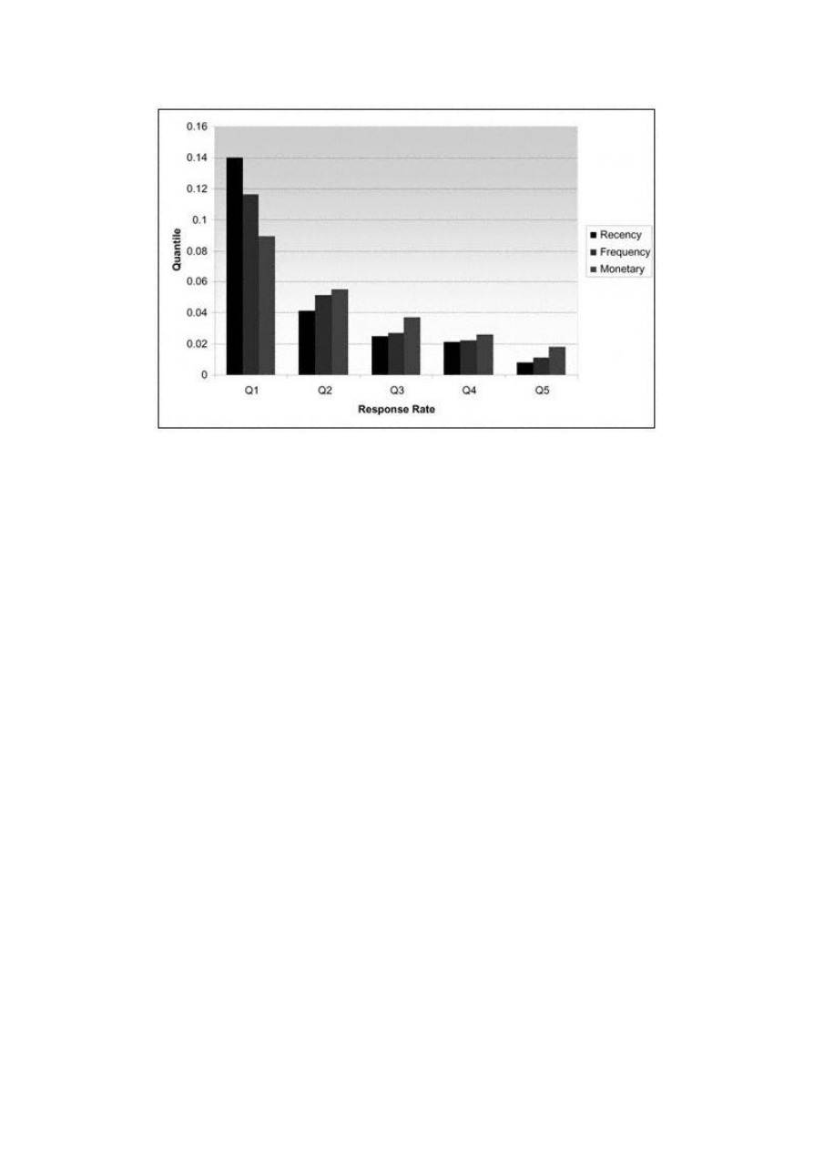
Page 194

Figure

8.3

Histogram

RFM

quintiles

response.

proc format;
value age
0-29 = ' < 30'
30-34 = '30-34'
35-39 = '35-39'
40-44 = '40-44'
45-49 = '45-49'
50-54 = '50-54'
55-64 = '55-64'
65-high = '65+'
;
value $gender
' ' = 'Unknown'
'M' = 'Male'
'F' = 'Female'
value count
. = 'Unknown'
0-2 = '0-2'
3-5 = '3-5'
6-10 = '6-10'
11->21 = '11-20'
21-high = '21-30'
;
run;

Page 195

proc freq data=ch08.customer;
format age age. length count.;
table age length /missing;
run;

Figure 8.4 shows the output from PROC FREQ for the first two variables. This gives us information about the
distribution of our customers. Notice how 33% of the customers are between the ages of 45 and 50. In order to make use
of this information for new acquisition marketing, we need to compare this finding to the general population. The next
PROC FREQ creates similar profiles for the general population:

proc freq data=ch08.pop;
format age age. length count.;
table age length /missing;
run;

Figure

8.4

Customer

profiles.

Page 196

Figure

8.5

Market

profiles.

Notice how Figure 8.5 displays the same distributions as Figure 8.4 except this time they are on the general population.
Figure 8.6 shows a market comparison graph of age. Table 8.1 brings the information from the two analyses together
and creates a measure called a penetration index. This is derived by dividing the customer percentage by the market
percentage for each group and multiplying by 100.

Figure 8.6 provides a graphical display of the differences in distribution for the various age groupings. SAM would be
wise to see new customers in the 35–44 age group. This age range is more prominent in its customer base than in the
general population.

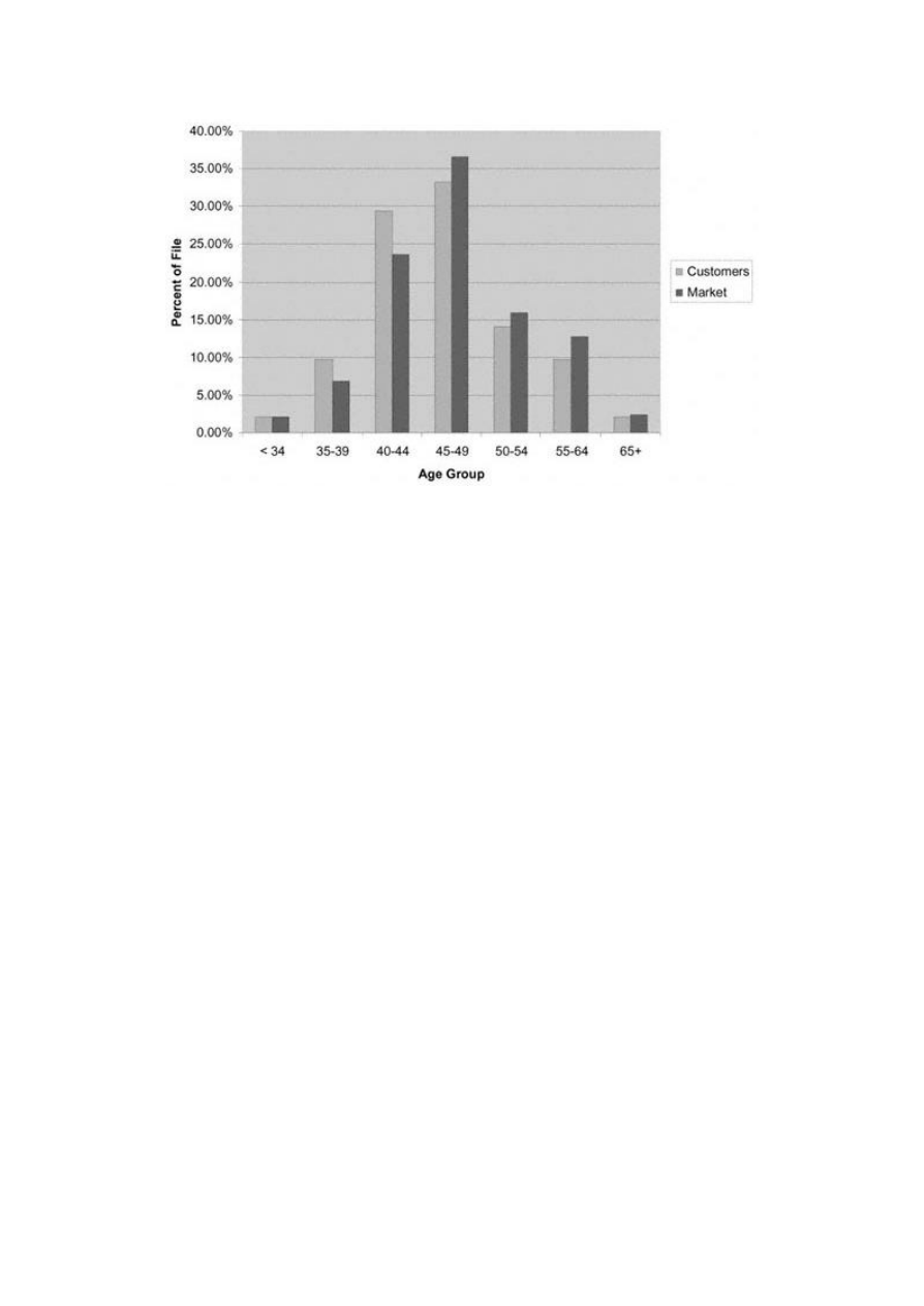
Page 197

Figure

8.6

Penetration

comparison

graph

age.

Table 8.1

Penetration Analysis

AGE

CUSTOMERS

PERCENT

CUSTOMERS

MARKET

PERCENT

MARKET

PENETRATO

INDEX

< 34

725

2.04%

117,062

2.06%

35–39

3,445

9.67%

387,464

6.81%

142

40–44

10,440

29.32%

1,341,725

23.58%

124

45–49

11,795

33.12%

2,084,676

36.63%

50–54

5,005

14.06%

900,779

15.83%

55–64

3,435

9.65%

726,869

12.77%

65+

765

2.15%

131,835

2.32%

Total

35,610

5,690,410

continues

Page 198

(Continued)

LENGTH

CUSTOMERS

PERCENT

CUSTOMERS

MARKET

PERCENT

MARKET

PENETRATION

INDEX

Unknown

0.21%

69,938

1.23%

0–2

10,135

28.46%

1,071,136

18.82%

151

3–5

9,090

25.53%

900,779

15.83%

161

6–10

9,785

27.48%

1,027,565

18.06%

152

11–20

6,035

16.95%

1,308,626

23.00%

21–30

490

1.38%

1,312,366

23.06%

Total

35,610

5,690,410

Developing a Customer Value Matrix for a Credit Card Company

Our second case study expands the use of profiling and segmentation to a customer view that reflects behavior as well as
demographics. Risk is a form of behavior that has implications in many industries. As we saw in our life insurance case
study in chapters 3 through 7, the risk of claims is a strong profit driver in the insurance industry. Credit card banks are
also vulnerable to the effect of risk. A slight increase in bankruptcies and charge -offs can quickly erode small profit
margins.

To understand our customer base with respect to revenue and risk, I perform a customer value analysis. This allows me
to segment the customer base with respect to profitability leading to improved customer relationship management.

Customer Value Analysis

Credit card profitability is achieved by balancing revenue (less costs) and risk. An effective way to segment the market
is by a combination of risk and net revenue. The first step is to determine the splitting values for risk and revenue. In this
case, I use $150 for revenue and 650 for risk. These values are not cast in stone. The revenue value of $150 represents
some revolving activity or high transaction activity. Accounts with revenues higher than $150 are worth considering for
more marketing efforts. The risk score of 650 corresponds to an average charge-off rate that the bank considers
tolerable. Accounts with scores below 650 are considered high risk.

Page 199

The following code uses PROC FORMAT to split the population into two groups by both revenue and risk:

proc format;
value revenue
low-<151 = 'Low Revenue'
151-high = 'High Revenue'
;
value risk
low-<651 = 'High Risk'
651-high = 'Low Risk'
;
run;

Next, I use PROC TABULATE to create a customer value matrix. The procedure uses the previous formats to split the
groups. The table statement crosses revenue (acctrev) by risk score (riskscr) with the number and percent of customers
(records):

proc tabulate data=ch08.profit;
format acctrev revenue. riskscr risk.;
class acctrev riskscr;
var records;
table (acctrev=' ' all='Total'),( riskscr=' ' all='Total')
*(records='#'*sum=' '*f=comma8. records='%'*pctsum=' '*f=8.2)
/rts=15 box='Customer Value Matrix';
run;

The results of the analysis are displayed in Figure 8.7. This matrix gives us an instant view of the customer database
with respect to revenue and risk. We see that over 66% are considered high revenue and almost 53% are low risk. Our
best customers, low risk and high revenue, make up 33% of our customer base.

Figure

8.7

Customer

value

matrix.

Page 200

The next step is to see what they look like. I will profile the customers within each segment.

The following data step creates a new variable called segment . This variable has a value for each of our four segments.
Following the data step, I format the segment values for use in our profile table:

data ch08.profit;
set ch08.profit;
if riskscr < 651 then do;
if acctrev < 151 then segment = '1' ;
else segment = '2';
end;
else do;
if acctrev < 151 then segment = '3' ;
else segment = '4';
end;
run;

proc format;
value $ segment
'1' = 'High Risk Low Revenue'
'2' = 'High Risk High Revenue'
'3' = 'Low Risk Low Revenue'
'4' = 'Low Risk High Revenue'
;
run;

Using PROC TABULATE, I profile each segment by finding the average values of selected demographic and behavioral
variables within each segment. The following code calculates the mean, minimum, and maximum for each selected
variable:

proc tabulate data=ch08.profit;
format segment $segment.;
class segment;
var records age length numkids income male riskscr acctrev;
table records='Total Customers'*sum=' '*f=comma9.
riskscr='Risk Score'*(mean='Mean'*f=comma5. min='Min'
*f=comma4. max='Max'*f=comma4.)
acctrev='Account Revenues'*(mean='Mean'*f=dollar6. min='Min'
*f=dollar5. max='Max'*f=dollar5.)
age='Age'*(mean='Mean'*f=comma5. min='Min'
*f=comma4. max='Max'*f=comma4.)
length='Length of Residence'*(mean='Mean'*f=comma5. min='Min'
*f=comma4. max='Max'*f=comma5.)
numkids='Number of Children'*(mean='Mean'*f=comma6.2 min='Min'
*f=comma4. max='Max'*f=comma4.)

Team-Fly

Page 201

income='Income (000)'*(mean='Mean'*f=dollar6. min='Min'
*f=dollar5. max='Max'*f=dollar5.)
male='Percent Male'*(mean='Mean'*f=percent6.2 min='Min'
*f=percent4. max='Max'*f=percent4.),
(segment=' ' all='Total')
/rts=30 box='Customer Profiles';
run;

In Figure 8.8, we see the variables across the rows and the segments in columns. This facilitates easy comparison of
different values within the groups. I like to check the extreme values (min and max) for irregularities.

Once I am comfortable with the range of the variables, I display the mean values only in a table that is useful for
developing marketing strategies. In Figure 8.9, the averages for each variable are displayed, and each segment is named
for its overall character.

Managers and marketers find this type of analysis very useful for developing marketing strategies. Let's look at each
segment separately:

Consummate consumers. These are the most profitable customers. They are low risk and generate high revenues.
Banks can use this knowledge to offer extra services and proactively offer lower rates in the face of steep competition.

Risky revenue. These are also profitable customers. Their main liability is that they are high risk. Many banks see this
as a reason to reduce balances. With higher pricing, though, these customers can be the most profitable because they are
less likely to attrite.

Business builders. These are the most challenging customers. They would be profitable if they carried balances, but
they tend to pay their full balance every month. Some in the industry call them the ''dreaded transactors." These
customers can sometimes be lured to revolve (carry balances) with low rates, but this can be a losing proposition for the
bank. Another option is to charge an annual fee. Some banks are successful with a creative blending of purchase
incentives and temporary low rates.

Balance bombs. No one wants these customers. They are risky and do not revolve balances. Some banks identify these
customers so they can reduce their credit lines and raise their interest rates to dissuade them from continuing the
relationship.

Every industry has drivers that can be effectively segmented. This simple exercise can provide direction and generate
ideas for improved customer profitability.

Page 202

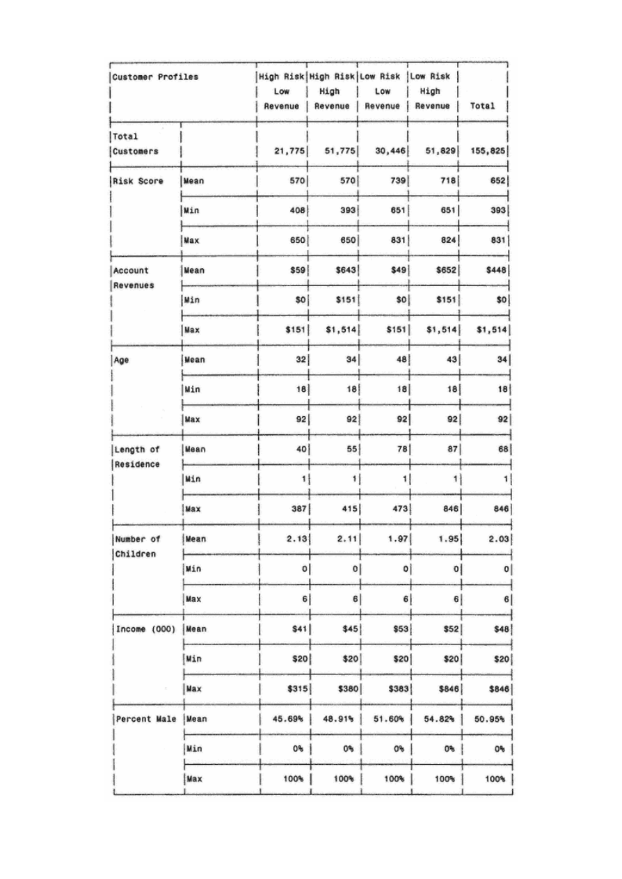
Figure

8.8

Customer

profiles

segment.

Page 203

Figure

8.9

Customer

profiles

segment,

simplified.

Performing Cluster Analysis to Discover Customer Segments

Cluster analysis is a family of mathematical and statistical techniques that divides data into groups with similar
characteristics. Recall that in chapter 4, I used frequencies to find similar groups within variable ranges. Clustering
performs a similar process but in the multivariate sense. It uses Euclidean distance to group observations together that
are similar across several characteristics, while attempting to separate observations that are dissimilar across those same
characteristics.

It is a process with many opportunities for guidance and interpretation. Several algorithms are used in clustering. In our
case study, I use PROC FASTCLUS. This is designed for use on large data sets. It begins by randomly assigning cluster
seeds or centers. The number of seeds is equal to the number of clusters requested. Each observation is assigned to the
nearest seed. The seed is then reassigned to the mean in each cluster. The process is repeated until the change in the seed
becomes sufficiently small.

To illustrate the methodology, I use two variables from the catalog data in our earlier case study. Before I run the cluster
analysis I must standardize the

Page 204

variables. Because the clustering algorithm I am using depends on distance between variable values, the scales of the
variables must be similar. Otherwise, the variable with the largest scale will dominate the clustering procedure. The
following code standardizes the variables using PROC STANDARD:

proc standard mean=0 std=1 out=stan;
var age income;
run;

The programming to create the clusters is very simple. I designate three clusters with random seeds (random=5555).
Replace=full directs the program to replace all the seeds with the cluster means at each step. I want to plot the results, so
I create an output dataset call outclus.

proc fastclus data=stan maxclusters=3 random=5555 replace=full
out=outclus;
var age income;
run;

In Figure 8.10, the output displays the distance from the seeds to the farthest point as well as the distances between
clusters. The cluster means do show a notable difference in values for age and income. For an even better view of the
clusters, I create a plot of the clusters using the following code:

proc plot;
plot age*income=cluster;
run;

The plot in Figure 8.11 shows three distinct groups. We can now tailor our marketing campaigns to each group
separately. Similar to the profile analysis, understanding the segments can improve targeting and provide insights for
marketers to create relevant offers.

Summary

In any industry, the first step to finding and creating profitable customers is determining what drives profitability. This
leads to better prospecting and more successful customer relationship management. You can segment and profile your
customer base to uncover those profit drivers using your knowledge of your customers, products, and markets. Or you
can use data-driven techniques to find natural clusters in your customer or prospect base. Whatever the method, the
process will lead to knowledge and understanding that is critical to maintaining a competitive edge.

Be on the lookout for new opportunities in the use of segmentation and profiling on the Internet. In chapter 13, I will
discuss some powerful uses for profiling, segmentation, and scoring on demand.

Page 205

Figure

8.10

Cluster

analysis

age

and

income.

Page 206

Figure

8.11

Plot

clusters

age

and

income.

Page 207

Chapter 9—
Targeting New Prospects:
Modeling Response

The first type of predictive model that most companies endeavor to use is the response model. Recall from chapter 1 that
a response model simply estimates the probability of response to an offer. Response is one of the easiest dynamics to
model and can be validated very quickly. In part 2, our case study predicted activation. But in the two-model approach, I
developed a model to predict response and another to predict activation given response. In this chapter, I will perform a
similar exercise. To provide a slightly different perspective, I will use a business-to-business example. Our case study
for this chapter involves predicting the propensity to respond to an offer to buy office supplies from an office supply
retail chain. I will use some predictive variables that are familiar. And I will introduce another group of variables that are
unique to business-to-business modeling. In addition, I will demonstrate how weights can be used to improve the results.
The actual modeling process will follow the same steps as were demonstrated in part 2.

Defining the Objective

Downing Office Products contracts with large companies to sell office supplies, office furniture, and technical
equipment. It also has many retails stores through which it collects information about its customers. It is interested in
increasing sales to new and existing customers through a combination of direct

Page 208

mail and telemarketing. Downing's marketing director decided to purchase business names and other company
information to develop a response model. The company also purchased census information with local demographic data
for each business on the list.

To build a response model, the data set needs to contain responders and nonresponders along with predictive information
about both groups. To get a pure data set for modeling, Downing would have to purchase a sample (or the entire file),
solicit the businesses, and model the results. Because many of Downing's customers were on the list, the decision was
made to build a propensity model. A propensity model is a model that predicts the propensity to take an action. In this
case, I want to build a model that predicts the propensity to respond to an offer to buy products from Downing.

To create the modeling data set, the Downing customer file was matched to the purchased list of business prospects. For
the names that matched, 12 -month sales figures were overlaid onto the file of business names. For Downing Office
Products, a response is defined as someone who buys office products.

The first step is to specifically define the dependent variable as someone with 12 -month sales (sales12mo ) greater than
zero:

data ch09.downing;
set ch09.downing;
if sale12mo > 0 then respond = 1; else respond = 0;
run;

Table 9.1 displays the result of the file overlay. Downing has already benefited from prior sales to over half of the
business list. Its goal is to leverage those relationships as well as develop new ones.

All Responders Are Not Created Equal

While I am interested in predicting who will respond, all responders are not alike. Some responders may spend less than
$100 a year while others spend many thousand of dollars. My real goal is to predict dollar sales, but that would require
using linear regression. Linear regression works best if the dependent variable, or the variable I am trying to predict, is
normally distributed. In our

Table 9.1

Downing Business List Frequency and Weights

GROUP

LIST

PERCENT

WEIGHT

Responders

26,306

51.5%

f(12-month sales)

Nonresponders

24,761

48.5%

Total

51,067

100%

Team-Fly

case, all the nonresponders have 12-monthe sales of zero. This would make it difficult to fit a model using linear
regression.

Instead, I can improve the results by using a weight to cause the model to favor the high spenders. It is important to note that the use of weights in
this case will distort the population. So the resulting model will not yield an accurate point estimate. In other words, the resulting probability will not
be an accurate estimate, but the file will still rank properly. If the model is built using weights, the highest spending responders should rank near the
top. This will become clearer as we work through the case study.

Because I am dealing with a binary outcome (response) with a meaningful continuous component (sales), I want to look at the distribution of sales.
The variable that represents 12-month sales is sale12mo. The following code produces the univariate output seen in Figure 9.1.

proc univariate data = ch09.downing plot;
where sale12mo > 0;
var sale12mo;
run;

The output in Figure 9.1 shows that over 50% of Downing's customers have 12-month sales of less than $100. And over 25% have 12
less than $50. To help the model target the higher-dollar customers, I will use a function of the sales amount as a weight.

Figure

9.1

Univariate

analysis

dependent

variable.

Page 210

As I mentioned previously, for responders I will define the weight as a function of the 12-month sales. The weights work
exactly as they did when I took a sample in the case study in part 2. The higher the weight, the more that observation is
represented in the file. It makes sense that if I use a function of the 12-month sales amount as a weight, the model
prediction will lean toward the higher-sales responders.

To create the weight for the responders, I am going to take the 12-month sales value divided by the average 12 -month
sales value for all responders. By using this fraction, I can create higher representation among the big spenders without
inflating the overall numbers in the sample. This will help to keep the coefficients in the normal range. The weight for
nonresponders is 1. The weight that is used to favor big spenders is called boostwgt. The following code creates
boostwght:

proc univariate data=ch09.downing noprint;
var sale12mo;
output out=wgtdata mean=s12mmean;
run;

data ch09.downing;
set ch09.downing;
if (_n_ = 1) then set wgtdata;
if respond = 1 then boostwgt = sale12mo/s12mmean;
else boostwgt = 1;
run;

I will use the weight boostwgt to assist in transforming the variables. This will help me find the form of the variable that
fits a model to target big spenders.

Preparing the Variables

As in our case study, the first step is to prepare the variables for entry into the model. The business data that was
purchased has more than 250 predictive variables. The first step is to perform some simple procedure to eliminate
weaker variables.

Continuous Variables

Many of these variables are numeric or continuous. Before I spend a lot of time looking at each variable individually, I
am going to put them all through a stepwise logistic with only one step. (This is the same technique I used in chapter 4.)
The first step defines the intercept. With the details option, I can look at the list of variables not in the model. This lists
the univariate chi -square or indi-

vidual predictive power of each variable. The following code, with an abbreviated variable list, is used to produce the univariate chi
values:

proc logistic data=ch09.downing descending;
weight boostwgt;
model respond = p1prshh p2prshh p3prshh pamsy —- pzafflu peduca pzincom
pzsesi /selection=stepwise maxstep=1 details;
run;

The output in Figure 9.2 shows the list of univariate chi -square values for each variable. Because I am using the weight, all the chi
are inflated. Of the 221 continuous variables examined, I select 33 of the most significant. These variables will be examined more closely.

The next step is to look for missing values and outliers. Because of the high number of variables, I use PROC
MEANS:

proc means data=ch09.downing n nmiss min mean max maxdec = 2;
weight boostwgt;
var pamsy pid80c4 pid80c8 plor2_5 pmobile —— pzsesi
;
run;

In Figure 9.3, the output from PROC MEANS shows two variables with missing values. In chapter 4 I discussed a number of ways to handle
missing values. Because that is not the emphasis of this chapter, I will just use mean substitution. For each variable, I also create a new variable to
identify which records have missing values. The following code replaces the missing values for pid80c4 and ppbluec and creates four new
variables , pid80crn, pc4_miss, ppbluecn, and pec_miss. (Note: I'm using the first and last two letters to create a three-character reference to each
variable.)

Figure

9.2

Univariate

chi -square.

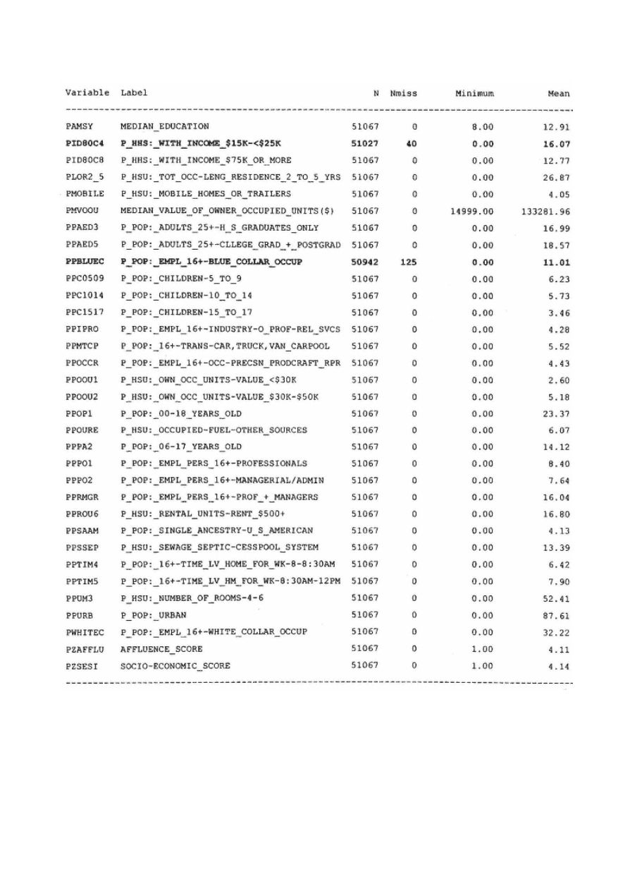
Figure

9.3

Means

analysis

continuous

variables.

data ch09.downing;
set ch09.downing;
if pid80c4 = . then do;
pid80c4n = 16.07;
pc4_miss = 1;
end;
else do;
pid80c4n = pid80c4;

pc4_miss = 0;
end;
if ppbluec = . then do;
ppbluecn = 11.01;
pec_miss = 1;
end;
else do;

Page 213

ppbluecn = ppbluec;
pec_miss = 0;
end;
run;

There do not appear to be any outliers, so I will begin transforming the variables. Recall the method in chapter 4. The
first step is to segment the continuous variables into 10 equal buckets. Then I look at a frequency analysis to see if there
are any obvious ways to segment the variable to create indicator (0/1) variables. The following code creates the buckets
and produces the frequency for the variable for median education, pamsy:

proc univariate data=ch09.downing noprint;
weight boostwgt;
var pamsy;
output out=psydata pctlpts= 10 20 30 40 50 60 70 80 90 100 pctlpre=psy;
run;

data freqs;
setch09.downing;
if (_n_ eq 1) then set psydata;
retain psy10 psy20 psy30 psy40 psy50 psy60 psy70 psy80 psy90 psy100;
run;

data freqs;
set freqs;
if pamsy < psy10 then psygrp10 = 1; else
if pamsy < psy20 then psygrp10 = 2; else
if pamsy < psy30 then psygrp10 = 3; else
if pamsy < psy40 then psygrp10 = 4; else
if pamsy < psy50 then psygrp10 = 5; else
if pamsy < psy60 then psygrp10 = 6; else
if pamsy < psy70 then psygrp10 = 7; else
if pamsy < psy80 then psygrp10 = 8; else
if pamsy < psy90 then psygrp10 = 9; else
psygrp10 = 10;
run;

proc freq data= freqs;
weight boostwgt;
table respond*psygrp10;
run;

In Figure 9.4, I see that the output gave us only 4 groups. I was expecting 10 groups. This is probably due to the limited
number of values for pamsy. In the next step, I print out the values for the different deciles of pamsy to see why I have
only 4 groups:

proc print data=psydata;
run;

Page 214

The following output validates my suspicions. The groupings in Figure 9.3 will work for our segmentation.

OBS PSY10 PSY20 PSY30 PSY40 PSY50 PSY60 PSY70 PSY80 PSY90
PSY100

1 12 12 12 12 12 13 13 14 16 18

Based on the response rates for the groups in Figure 9.3, I will create two binary variables by segmenting pamsy at the
values for PSY60 and PSY90. When you look at the column percent for respond = 1, you'll notice that as the values for
pamsy increase, the response percents have a nice upward linear trend, so the continuous form may be more powerful.
We will look at that in the next step.

data ch09.downing;
set ch09.downing;
if pamsy < 13 then pamsy13 = 1; else pamsy13 = 0;
if pamsy < 16 then pamsy16 = 1; else pamsy16 = 0;
run;

Figure

9.4

Segmentation

analysis.

Page 215

Again going back to the techniques in chapter 4, I use a quick method to determine the best transformation for the
continuous variables. First, I transform pamsy using a variety of functions. Then I use logistic regression with the
selection=stepwise maxstep = 2 options to find the best fitting transformation:

data ch09.downing;
set ch09.downing;

psy_sq = pamsy**2; /*squared*/
psy_cu = pamsy**3; /*cubed*/
psy_sqrt = sqrt(pamsy); /*square root*/
psy_curt = pamsy**.3333; /*cube root*/
psy_log = log(max(.0001,pamsy)); /*log*/
psy_exp = exp(max(.0001,pamsy)); /*exponent*/

psy_tan = tan(pamsy); /*tangent*/
psy_sin = sin(pamsy); /*sine*/
psy_cos = cos(pamsy); /*cosine*/

psy_inv = 1/max(.0001,pamsy); /*inverse*/
psy_sqi = 1/max(.0001,pamsy**2); /*squared inverse*/
psy_cui = 1/max(.0001,pamsy**3); /*cubed inverse*/
psy_sqri = 1/max(.0001,sqrt(pamsy)); /*square root inv*/
psy_curi = 1/max(.0001,pamsy**.3333); /*cube root inverse*/

psy_logi = 1/max(.0001,log(max(.0001,pamsy))); /*log inverse*/
psy_expi = 1/max(.0001,exp(max(.0001,pamsy))); /*exponent inv*/

psy_tani = 1/max(.0001,tan(pamsy)); /*tangent inverse*/
psy_sini = 1/max(.0001,sin(pamsy)); /*sine inverse*/
psy_cosi = 1/max(.0001,cos(pamsy)); /*cosine inverse*/

run;

proc logistic data=ch09.downing descending;
weight boostwgt;
model respond = pamsy pamsy13 pamsy16 psy_sq psy_cu psy_sqrt psy_curt
psy_log psy_exp psy_tan psy_sin psy_cos psy_inv psy_sqi psy_cui psy_sqri
psy_curi psy_logi psy_expi psy_tani psy_sini psy_cosi / selection = step-
wise maxstep=2 details;
run;

In Figure 9.5, we see the results of the stepwise logistic on pamsy. The two strongest forms are the natural form, psy_sq
and pamsy13 (pamsy < 13). These two forms will be candidates for the final model.

This process is repeated for the remaining 32 variables. The winning transformations for each continuous variable are
combined into a new data set called acqmod.down_mod;

Figure

9.5

Variable

transformation

selection.

Table 9.2 is a summary of the continuous variables and the transformations that best fit the objective function.

The next step is to analyze and prepare the categorical variables.

Table 9.2

Summary of continuous Variable Transformations

VARIABLE

PREFIX

SEGMENTS

TRANSFORMATION 1

TRANSFORMATION 2

DESCRIPTION

pamsy

psy

''< 12, 13, 14, 16"

pamsy13

Median Education

pid80c4

pc4

sqrt

cui

Income $15K

pid80c8

pc8

<5.1

sqrt

logi

Income $75K+

plor2_5

p_5

as is

tan

Length of

Residence

2-5 Years

(table continued on next page)

Team-Fly

(table continued from previous page)

VARIABLE

PREFIX

SEGMENTS

TRANSFORMATION 1

TRANSFORMATION 2

DESCRIPTION

pmobile

ple

<.5

curt

Mobile Homes in Area

pmvoou

pou

<65600

sqrt

cui

Median Value of

Home

ppaed3

pd3

<21.3

as is

low

% 25+ Years & High

School Grad

ppaed5

pd5

sqrt

curt

% 25+ Years &

College Grad

ppbluec

pec

<9.4

as is

low

% 16+ Years Blue

Collar

ppc0509

p09

< 6.9 & < 7.3

as is

% w/Children 5

ppc1014

p14

as is

% w/Children 10

ppc1517

p17

< 4.1

as is

% w/Children 15

ppipro

pro

curt

cosi

% Empl 16+ Years

Industry Services

ppmtcp

pcp

< 7.3

sqrt

curi

"% Trans: Car, Van

Truck, Carpool"

ppoccr

pcr

< 4.9

sqrt

tani

% Empl 16+ Years

Product Craft

ppoou1

pu1

curt

tan

% Homes Valued <

$30K

ppoou2

pu2

< 14.1

curt

tan

% Homes Valued

$30K–$

ppop1

pp1

as is

% 0–18 Years Old

ppoure

pre

< 2.1 >18.9

med

sqrt

% Occupied Full

Other Sources

pppa2

pa2

as is

% 6–17 Years Old

pppo1

po1

< 4.8

sqrt

logi

% Empl 16+ Years

Professional

pppo2

po2

as is

logi

% Empl 16+ Years

Managerial

continues

(Continued)

VARIABLE

PREFIX

SEGMENTS

TRANSFORMATION 1

TRANSFORMATION 2

DESCRIPTION

pprmgr

pgr

< 10.3

as is

logi

% Empl 16+ Years Prof

& Managerial

pprou6

pu6

curt

logi

% Rental Units w/ Rent

$500+

ppsaam

pam

< 6.8

as is

cosi

% Single Ancestry

American

ppssep

pep

curt

cui

% Sewage/Cesspool/

Septic System

pptim4

pm4

as is

sin

% Pop Leave for Work

8–8:30 AM

pptim5

pm5

< 4.3

curt

logi

% Pop Leave for Work

8–12:00 AM

ppum3

pm3

% Number of Rooms 4

ppurb

prb

cos

% Urban

pwhitec

ptc

< 19.6

log

% Employee 16+ White

Collar

pzafflu

plu

< 7

low

sqrt

Affluence Score

pzsesi

psi

sqrt

cosi

Socio-Economic Score

Categorical Variables

As discussed in Chapter 4, logistic regression uses only numeric variables. And it sees all variables as continuous. In order to use
categorical variables, I must create indicator, or binary, variables to state whether a given situation is true or false.

I have 15 categorical variables. The first step is to run a frequency against the weighted response variable. I also request the missing
option and a chi -square test of significance:

proc freq data=ch09.down_mod;
weight boostwgt;
table respond*(buslevel subsidcd heircode strucode afflcode poprange

Page 219

geogarea emplsize indscode mfglocal legalsta mktbilty offequip whitcoll
printer)/ chisq missing;
run;

Figure 9.6 displays the output for the first variable, buslevel . It shows that each value for buslevel has a significantly
different response rate.

The values for this variable represent the status of the business. The following list details the values: 0 = Single Entity; 1
= Headquarters; 2 = Branch. To capture the values, I create two indicator variables, bus_sgle and bus_hdqt, each

Figure

9.6

Frequency

business

level

weighted

response.

Page 220

having the values of 0 and 1. If they are both equal to 0, then the value = 2 or Branch.

I run frequencies for all categorical variables and analyze the results. I create indicator variables for each categorical
variable to capture the difference in weighted response. The following code creates indicator (0/1) variables for all
categorical variables in the final model:

data ch09.down_mod;
set ch09.down_mod;

bus_sgle = (buslevel = '0');
bus_hdqt = (buslevel = '1');

subsudz = (subsidcd = '3');

heir_mis = (heircode = ' ');

autonent = (strucode = 'AE');
branch = (strucode = 'BR');
sub_head = (strucode = 'SH');
subsid = (strucode = 'SU');

multaffl = (afflcode = '0');
pop_high = (poprange in (' ', '0'));
pop_num = max(0, poprange);

geog_low = (geogarea in ('04','07','10'));

empl_100 = (emplsize = 'A');
empl_500 = (emplsize = 'E');
empl1000 = (emplsize = 'R');

ind_high = (indscode in ('A','B','C','L','N','U','Y'));
ind_low = (indscode in ('D','J','T','Z'));

mfgloc_y = (mfglocal = 'Y');
mfgloc_n = (mfglocal = 'N');

offequ_y = (offequip = 'Y');

whiteco1 = (whitcoll in (' ','A'));
whiteco2 = (whitcoll in ('B','C'));

print_h = (printer = 'C');
run;

Page 221

Processing the Model

I now have a full list of candidate variables. As I did in part 2, I am running logistic regression with three different
selection options. First, I will run the backward and stepwise selection on all variables. I will then take the combination
of winning variables from both methods and put it into a logistic regression using the score selection. I will begin
looking at models with about 20 variables and find where the score increase begins to diminish with each new variable.

The following code processes the backward selection procedure. The first section of code splits the file into modeling
and validation data sets. Due to the large number of variables, I used the option sls=.0001. This keeps only the variables
whose level of significance is very high. In other words, the probability that the variable is not truly predictive is less
than .0001:

data ch09.down_mod;
set ch09.down_mod;
if ranuni(5555) < .5 then splitwgt = 1;
else splitwgt = .;

modwgt = splitwgt*boostwgt;
records=1;
run;

proc logistic data=ch09.down_mod descending;
weight modwgt;
model respond = AUTONENT BUS_HDQT BUS_SGLE EMPL1000 EMPL_100 EMPL_500
GEOG_LOW HEIR_MIS IND_HIGH IND_LOW MFGLOC_N MFGLOC_Y MULTAFFL OFFEQU_Y
P09_CU P14_CU P17_CU PA2_CU PAMSY13 PSY_SQ PC4_CUI PC4_SQRT
PC8_LOGI PC8_SQRT PCR_SQRT PCR_TANI PD3_LOW PD5_CURT PD5_SQRT PEC_LOW
PEP_CUI PEP_CURT PGR_LOGI PID80C4 PID80C8 PLE_CU PLE_CURT PLOR2_5
PLU_LOW PLU_SQRT PM3_CU PM4_SIN PM5_CURT PM5_LOGI PMOBILE PMVOOU
PO1_LOGI PO1_SQRT PO2_LOGI POP_HIGH POP_NUM POU_CUI POU_SQRT PP1_CU
PPAED3 PPAED5 PPBLUEC PPC0509 PPC1014 PPC1517 PPIPRO PPMTCP
PPOCCR PPOOU1 PPOOU2 PPOP1 PPOURE PPPA2 PPPO1 PPPO2
PPRMGR PPROU6 PPSAAM PPSSEP PPTIM4 PPTIM5 PPUM3 PPURB
PRB_COS PRB_CU PRE_MED PRE_SQRT PRINT_H PRO_COSI PRO_CURT PSI_COSI
PSI_SQRT PTC_LOG PTC_SQ PU1_CURT PU1_TAN PU2_CURT PU2_TAN PU6_CURT
PU6_LOGI PWHITEC PZAFFLU PZSESI P_5_TAN SUBSUDZ WHITECO1 WHITECO2
/selection=backward sls=.0001;
run;

The next code performs a logistic regression on the same variables with the selection=stepwise option. In this model, I
used the options, sle=.0001 and sls=.0001. These options specify the level of significance to enter and stay in the model.

Page 222

proc logistic data=ch09.down_mod descending;
weight modwgt;
model respond = AUTONENT BRANCH BUS_HDQT EMPL1000 EMPL_100
EMPL_500
| | | | | | |
| | | | | | |
PU6_LOGI P_5_TAN SUBSUDZ WHITECO1 WHITECO2
/selection=stepwise sle=.0001 sls=.0001;
run;

As I expect, the backward selection has many more variables. But the stepwise selection has five variables that were not
selected by the backward selection method, ppipro , pm3_cu, pppa2, ptc_sq, and pu1_curt. I add these five variables to
the list and run the logistic regression using the score selection. I want the best model based on the highest score so I use
the option, best=1;

proc logistic data=ch09.down_mod descending;
weight modwgt;
model respond = AUTONENT BUS_HDQT EMPL1000 EMPL_100 EMPL_500 GEOG_LOW
IND_HIGH IND_LOW MFGLOC_N MFGLOC_Y MULTAFFL PA2_CU PAM_SQ PC8_SQRT
PD3_LOW PD5_CURT PD5_SQRT PEC_LOW PEP_CUI PGR_LOGI PLE_CU PLE_CURT
PLU_LOW PM3_CU PPIPRO PPPA2 PTC_SQ PU1_CURT PM5_CURT PM5_LOGI
PMOBILE PMVOOU PO2_LOGI POP_HIGH POP_NUM POU_CUI POU_SQRT PP1_CU
PPAED3 PPAED5 PPBLUEC PPC1517 PPMTCP PPOCCR PPOOU1 PPOP1
PPPO1 PPRMGR PPROU6 PPURB PRB_COS PRB_CU PRE_MED PRE_SQRT
PRINT_H PSI_SQRT PU2_CURT PU6_CURT PU6_LOGI PZAFFLU PZSESI SUBSUDZ
WHITECO1 WHITECO2 /selection = score best=1;
run;

Figure 9.7 shows an abbreviated output from the logistic with selection=score. I look for a point where the amount of
increase in score starts to diminish. I end up selecting a model with 30 variables. I rerun these variables in a regular
logistic to create an output data set that contains the predicted values. My goal is to create a gains table so that I can
evaluate the model's ability to rank responders and 12-month sales. The following code runs the logistic regression,
creates an output scoring file (ch09.coeff), creates deciles, and builds a gains table. Notice that I do not use the weight in
the validation gains table:

proc logistic data=ch09.down_mod descending outest=ch09.coeff;
weight modwgt;
model respond = AUTONENT BUS_HDQT EMPL1000 EMPL_100 IND_HIGH IND_LOW
MFGLOC_N MFGLOC_Y MULTAFFL PA2_CU PC8_SQRT PD5_SQRT PEC_LOW PEP_CUI
PLU_LOW PM5_CURT PM5_LOGI PO2_LOGI POP_HIGH POP_NUM PPC1517 PPMTCP
PPOOU1 PPPA2 PRB_COS PRE_MED PRINT_H PU6_LOGI PZAFFLU SUBSUDZ WHITECO1
WHITECO2
output out=ch09.scored(where=(splitwgt=.)) p=pred;
run;

proc sort data=ch09.scored;

Figure

9.7

Logistic

regression

using

score

selection.

by descending pred;
run;

proc univariate data=ch09.scored noprint;
var records;
output out=preddata sum=totrec;
run;

data ch09.scored;
set ch09.scored;
if (_n_ eq 1) then set preddata;
retain totrec;
number+1;
if number < .1*totrec then val_dec = 0; else

if number < .2*totrec then val_dec = 1; else
if number < .3*totrec then val_dec = 2; else
if number < .4*totrec then val_dec = 3; else
if number < .5*totrec then val_dec = 4; else

Page 224

if number < .6*totrec then val_dec = 5; else
if number < .7*totrec then val_dec = 6; else
if number < .8*totrec then val_dec = 7; else
if number < .9*totrec then val_dec = 8; else
val_dec = 9;
run;

proc tabulate data=ch09.scored;
class val_dec;
var respond sale12mo pred records;
table val_dec='Decile' all='Total',
records='Prospects'*sum=' '*f=comma10.
pred='Predicted Probability'*mean=' '*f=11.5
respond='Percent Respond'*mean=' '*f=11.5
sale12mo='Sales'*sum=' '*f=dollar11. /rts = 9 row=float;
run;

Figure 9.8 shows the listing of parameter estimates for the final model. The most predictive variables are shown in bold.
These can be used to assist in solicitation design and other marketing decisions. The validation gains table created in
proc tabulate can be seen in Figure 9.9. These values are expanded into a spreadsheet that can be seen in Figure 9.10.
This table calculates cumulative values for response, 12-month sale, and lift. Notice how the lift is much greater for 12-
months sales than it is for lift. Again, this is a direct result of the weighting used to attract big-spending responders.

In Figure 9.9 the model shows good rank ordering of prospects by response and sales. The deciles are all monotonically
decreasing with a strong decline, especially in 12-month sales. In Figure 9.10 the cumulative values and lift measures
show the true power of this model. Notice how the lift for sales is so much better than the lift for response. This is a
result of the weighting.

Figure 9.10 also provides a wealth of information for making marketing decisions. As we did in chapter 7, we can use
this table to decide how many deciles we want to solicit. For example, if we want target businesses with greater than
$100 in sales, we would solicit through decile 5.

Figure 9.11 provides a visual account of the power of the model. Notice how the curve for 12-month sales is higher than
the curve for response. This reflects the higher lift in the prediction of 12-month sales.

Validation Using Boostrapping

As I discussed in chapter 6, an excellent method for determining the robustness of your model is to create bootstrap
samples and calculate confidence inter-

Figure

9.8

Parameter

estimates.

vals. The following code is a variation on the code in chapter 6. It calculates confidence intervals for response, 12-month sales
sales. The program uses some macro language to reduce the amount of code. The first step creates a small sample to speed processing. Since my
sample weight is artificial, I need to create a false sample weight equal to 1. This prevents having to change the program:

data ch09.bs_all;
set ch09.scored(keep= pred respond splitwgt records sale12mo val_dec);
smp_wgt=1;
run;

I use PROC UNIVARIATE to get the overall mean values for respond (rspmean) and 12-month sales (salmean).

proc univariate data=ch09.bs_all noprint;
weight smp_wgt;
var respond sale12mo;
output out=preddata sumwgt=sumwgt mean= rspmean salmean;
run;

Team-Fly

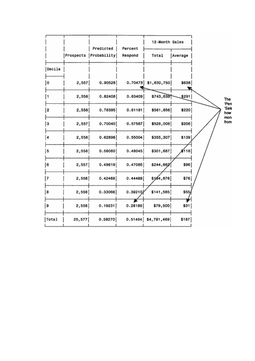
Figure

9.9

Validation

decile

analysis.

Figure

9.10

Validation

gains

table

with

lift.

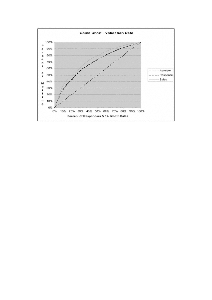
Page 227

Figure

9.11

Validation

gains

chart.

The following data step appends the overall mean values to every record:

data ch09.bs_all;
set ch09.bs_all;
if (_n_ eq 1) then set preddata;
retain sumwgt rspmean salmean;
run;

PROC SUMMARY creates mean values of respond (rspmnf) and 12-month sales (salmnf) for each decile (val_dec):

proc summary data=ch09.bs_all;
var respond sale12mo;
class val_dec;
output out=ch09.fullmean mean= rspmnf salmnf ;
run;

The next data step uses the output from PROC SUMMARY to create a separate data set (salfmean) with the two overall
mean values renamed. The overall mean values are stored in the observation where val_dec has a missing value ( val_dec
= .). These will be used in the final bootstrap calculation:

Page 228

data salfmean( rename=(salmnf=salomn_g rspmnf=rspomn_g ) drop=val_dec);
set ch09.fullmean( where=(val_dec=.) keep=salmnf rspmnf val_dec);
smp_wgt=1;
run;

In the next data step, the means are appended to every value of the data set ch09.fullmean. This will be accessed in the
final calculations following the macro.

data ch09.fullmean;
set ch09.fullmean;
if (_n_ eq 1) then set salfmean;
retain salomn_g rspomn_g;
run;

The bootstrapping program is identical to the one in chapter 6 up to the point where the estimates are calculated. The
following data step merges all the bootstrap samples and calculates the bootstrap estimates:

data ch09.bs_sum(keep=liftf bsest_r rspmnf lci_r uci_r bsest_s salmnf
lci_s uci_s bsest_l lftmbs lci_l uci_l val_dec salomn_g);
merge ch09.bsmns1 ch09.bsmns2 ch09.bsmns3 ch09.bsmns4 ch09.bsmns5
ch09.bsmns6 ch09.bsmns7 ch09.bsmns8 ch09.bsmns9 ch09.bsmns10
ch09.bsmns11 ch09.bsmns12 ch09.bsmns13 ch09.bsmns14 ch09.bsmns15
ch09.bsmns16 ch09.bsmns17 ch09.bsmns18 ch09.bsmns19 ch09.bsmns20
ch09.bsmns21 ch09.bsmns22 ch09.bsmns23 ch09.bsmns24 ch09.bsmns25
ch09.fullmean;
by val_dec;
rspmbs = mean(of rspmn1 -rspmn25); /* mean of response */
rspsdbs = std(of rspmn1 -rspmn25); /* st dev of response */

salmbs = mean(of salmn1 -salmn25); /* mean of sales */
salsdbs = std(of salmn1 -salmn25); /* st dev of sales */

lftmbs = mean(of liftd1 -liftd25); /* mean of lift */
lftsdbs = std(of liftd1 -liftd25); /* st dev of lift */

liftf = 100*salmnf/salomn_g; /* overall lift for sales */

bsest_r = 2*rspmnf - rspmbs; /* boostrap est - response */
lci_r = bsest_r - 1.96*rspsdbs; /* lower conf interval */
uci_r = bsest_r + 1.96*rspsdbs; /* upper conf interval */

bsest_s = 2*salmnf - salmbs; /* boostrap est - sales */
lci_s = bsest_s - 1.96*salsdbs; /* lower conf interval */
uci_s = bsest_s + 1.96*salsdbs; /* upper conf interval */

bsest_l = 2*liftf - lftmbs; /* boostrap est - lift */
lci_l = bsest_l - 1.96*lftsdbs; /* lower conf interval */
uci_l = bsest_l + 1.96*lftsdbs; /* upper conf interval */
run;

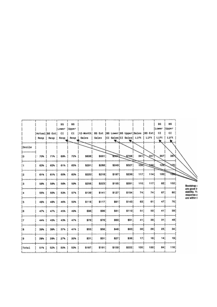
Finally, I use PROC TABULATE to display the bootstrap and confidence interval values by decile.

proc tabulate data=ch09.bs_sum;
var liftf bsest_r rspmnf lci_r uci_r bsest_s salmnf
lci_s uci_s bsest_l lftmbs lci_l uci_l;
class val_dec;
table (val_dec='Decile' all='Total'),
(rspmnf='Actual Resp'*mean=' '*f=percent6.
bsest_r='BS Est Resp'*mean=' '*f=percent6.
lci_r ='BS Lower CI Resp'*mean=' '*f=percent6.
uci_r ='BS Upper CI Resp'*mean=' '*f=percent6.

salmnf ='12-Month Sales'*mean=' '*f=dollar8.
bsest_s='BS Est Sales'*mean=' '*f=dollar8.
lci_s ='BS Lower CI Sales'*mean=' '*f=dollar8.
uci_s ='BS Upper CI Sales'*mean=' '*f=dollar8.

liftf ='Sales Lift'*mean=' '*f=6.
bsest_l='BS Est Lift'*mean=' '*f=6.
lci_l ='BS Lower CI Lift'*mean=' '*f=6.
uci_l ='BS Upper CI Lift'*mean=' '*f=6.)
/rts=10 row=float;
run;

Figure

9.12

Bootstrap

analysis.

Page 230

The results of the bootstrap analysis give me confidence that the model is stable. Notice how the confidence intervals are
fairly tight even in the best decile. And the bootstrap estimates are very close to the actual value, providing additional
security. Keep in mind that these estimates are not based on actual behavior but rather a propensity toward a type of
behavior. They will, however, provide a substantial improvement over random selection.

Implementing the Model

In this case, the same file containing the score will be used for marketing. The marketing manager at Downing Office
Products now has a robust model that can be used to solicit businesses that have the highest propensity to buy the
company's products.

The ability to rank the entire business list also creates other opportunities for Downing. It is now prepared to prioritize
sales efforts to maximize its marketing dollar. The top scoring businesses (deciles 7–9) are targeted to receive a personal
sales call. The middle group (4–8) is targeted to receive several telemarketing solicitations. And the lowest group
(deciles 0–3) will receive a postcard directing potential customers to the company's Web site. This is expected to provide
a substantial improvement in yearly sales.

Summary

Isn't it amazing how the creative use of weights can cause those high spenders to rise to the top? This case study is an
excellent example of how well this weighting technique works. You just have to remember that the estimated
probabilities are not accurate predictors. But the ability of the model to rank the file from most profitable to least
profitable prospects is superior to modeling without weights. In addition, the mechanics of working with business data
are identical to those of working with individual and household data.

Response models are the most widely used and work for almost any industry. From banks and insurance companies
selling their products to phone companies and resorts selling their services, the simplest response model can improve
targeting and cut costs. Whether you're targeting individuals, families, or business, the rules are the same: clear
objective, proper data preparation, linear predictors, rigorous processing, and thorough validation. In our next chapter,
we try another recipe. We're going to predict which prospects are more likely to be financially risky.

Page 231

Chapter 10—
Avoiding High-Risk Customers:
Modeling Risk

Most businesses are interested in knowing who will respond, activate, purchase, or use their services. As we saw in our
case study in part 2, many companies need to manage another major component of the profitability equation, one that
does not involve purchasing or using products or services. These businesses are concerned with the amount of risk they
are taking by accepting someone as a customer. Our case study in part 2 incorporated the effect of risk on overall
profitability for life insurance. Banks assume risk through loans and credit cards, but other business such as utilities and
telcos also assume risk by providing products and services on credit. Virtually any company delivering a product or
service with the promise of future payment takes a financial risk.

In this chapter, I start off with a description of credit scoring, its origin, and how it has evolved into risk modeling. Then
I begin the case study in which I build a model that predicts risk by targeting failure to pay on a credit-based purchase
for the telecommunications or telco industry. (This is also known as an approval model.) As in chapter 9, I define the
objective, prepare the variables, and process and validate the model. You will see some similarities in the processes, but
there are also some notable differences due to the nature of the data. Finally, I wrap up the chapter with a brief
discussion of fraud modeling and how it's being used to reduce losses in many industries.

Page 232

Credit Scoring and Risk Modeling

If you've ever applied for a loan, I'm sure you're familiar with questions like, ''Do you own or rent?" "How long have
you lived at your current address?" and "How many years have you been with your current employer?" The answers to
these questions— and more— are used to calculate your credit score. Based on your answers (each of which is assigned a
value), your score is summed and evaluated. Historically, this method has been very effective in helping companies
determine credit worthiness.

Credit scoring began in the early sixties when Fair, Isaac and Company developed the first simple scoring algorithm
based on a few key factors. Until that time, decisions to grant credit were primarily based on judgment. Some companies
were resistant to embrace a score to determine credit worthiness. As the scores proved to be predictive, more and more
companies began to use them.

As a result of increased computer power, more available data, and advances in technology, tools for predicting credit
risk have become much more sophisticated. This has led to complex credit scoring algorithms that have the ability to
consider and utilize many different factors. Through these advances, risk scoring has evolved from a simple scoring
algorithm based on a few factors to the sophisticated scoring algorithms we see today.

Over the years, Fair, Isaac scores have become a standard in the industry. While its methodology has been closely
guarded, it recently published the components of its credit-scoring algorithm. Its score is based on the following
elements:

Past payment history

•

Account payment information on specific types of accounts (e.g., credit cards, retail accounts, installment loans,

finance company accounts, mortgage)

•

Presence of adverse public records (e.g., bankruptcy, judgments, suits, liens, wage attachments), collection items,

and/or delinquency (past due items)

•

Severity of delinquency (how long past due)

•

Amount past due on delinquent accounts or collection items

•

Time since (recency of) past due items (delinquency), adverse public records (if any), or collection items (if any)

•

Number of past due items on file

Page 233

•

Number of accounts paid as agreed

Amount of credit owing

•

Amount owing on accounts

•

Amount owing on specific types of accounts

•

Lack of a specific type of balance, in some cases

•

Number of accounts with balances

•

Proportion of credit lines used (proportion of balances to total credit limits on certain types of revolving accounts)

•

Proportion of installment loan amounts still owing (proportion of balance to original loan amount on certain types of

installment loans)

Length of time credit established

•

Time since accounts opened

•

Time since accounts opened, by specific type of account

•

Time since account activity

Search for and acquisition of new credit

•

Number of recently opened accounts, and proportion of accounts that are recently opened, by type of account

•

Number of recent credit inquiries

•

Time since recent account opening(s), by type of

account

•

Time since credit inquiry(s)

•

Reestablishment of positive credit history following past payment problems

Types of credit established

•

Number of (presence, prevalence, and recent information on) various types of accounts (credit cards, retail accounts,

installment loans, mortgage, consumer finance accounts, etc.)

Over the past decade, numerous companies have begun developing their own risk scores to sell or for personal use. In
this case study, I will develop a risk score that is very similar to those available on the market. I will test the final scoring
algorithm against a generic risk score that I obtained from the credit bureau.

Page 234

Defining the Objective

Eastern Telecom has just formed an alliance with First Reserve Bank to sell products and services. Initially, Eastern
wishes to offer cellular phones and phone services to First Reserve's customer base. Eastern plans to use statement
inserts to promote its products and services, so marketing costs are relatively small. Its main concern at this point is
managing risk.

Since payment behavior for a loan product is highly correlated with payment behavior for a product or service, Eastern
plans to use the bank's data to predict financial risk over a three-year period. To determine the level of risk for each
customer, Eastern Telecom has decided to develop a model that predicts the probability of a customer becoming 90+
days past due or defaulting on a loan within a three-year period.

To develop a modeling data set, Eastern took a sample of First Reserve's loan customers. From the customers that were
current 36 months ago, Eastern selected all the customers now considered high risk or in default and a sample of those
customers who were still current and considered low risk. A high-risk customer was defined as any customer who was
90 days or more behind on a loan with First Reserve Bank. This included all bankruptcies and charge-offs. Eastern
created three data fields to define a high -risk customer: bkruptcy to denote if they were bankrupt, chargoff to denote if
they were charged off, and dayspdue, a numeric field detailing the days past due.

A file containing name, address, social security number, and a match key (idnum) was sent to the credit bureau for a data
overlay. Eastern requested that the bureau pull 300+ variables from an archive of 36 months ago and append the
information to the customer file. It also purchased a generic risk score that was developed by an outside source.

The file was returned and matched to the original extract to combine the 300+ predictive variables with the three data
fields. The following code takes the combined file and creates the modeling data set. The first step defines the
independent variable, highrisk. The second step samples and defines the weight, smp_wgt. This step creates two
temporary data sets, hr and lr, that are brought together in the final step to create the data set ch10.telco:

data ch10.creddata;
set ch10.creddata;
if bkruptcy = 1 or chargoff = 1 or dayspdue => 90 then highrisk = 1;
else highrisk = 0;
run;

data hr lr(where=(ranuni(5555) < .14));
set ch10.creddata;

Team-Fly

Page 235

if highrisk = 1 then do;
smp_wgt=1;
output hr;
end;
else do;
smp_wgt=7;
output lr;
end;
run;

data ch10.telco;
set hr lr;
run;

Table 10.1 displays the original population size and percents, the sample size, and the weights: The overall rate of high-
risk customers is 3.48%. This is kept intact by the use of weights in the modeling process. The next step is to prepare the
predictive variables.

Table 10.1 Population and Sample Frequencies and Weights

GROUP

POPULATION

PERCENT

SAMPLE

WEIGHT

High Risk

10,875

3.48%

10,875

Low Risk

301,665

96.5%

43,095

TOTAL

312,540

100%

53,970

The overall rate of high-risk customers is 3.48%. This is kept intact by the use of weights in the modeling process. The
next step is to prepare the predictive variables.

Preparing the Variables

This data set is unusual in that all the predictive variables are continuous except one, gender. Because there are so many
(300+) variables, I have decided to do things a little differently. I know that when data is sent to an outside source for
data overlay that there will be missing values. The first thing I want to do is determine which variables have a high
number of missing values. I begin by running PROC MEANS with an option to calculate the number of missing values,
nmiss. To avoid having to type in the entire list of variable names, I run a PROC CONTENTS with a short option. This
creates a variable list (in all caps) without any numbers or extraneous information. This can be cut and pasted into open
code:

proc contents data=ch10.telco short;
run;

proc means data=ch10.telco n nmiss mean min max maxdec=1;

var AFADBM AFMAXB AFMAXH AFMINB AFMINH AFOPEN AFPDBAL AFR29 AFR39 . . .
. .
. . . . . . . . . . . . . . . . UTR4524 UTR7924 UTRATE1 UTRATE2 UTRATE3;
run;

Figure 10.1 displays a portion of the results of PROC MEANS. Remember, there are 300+ variables in total, so my first goal is to look for an effective
way to reduce the number of variables. I decide to look for variables with good coverage of the data by selecting variables with less than 1,000 missing
values. There are 61 variables that meet this criterion.

With 61 variables, I am going to streamline my techniques for faster processing. The first step is to check the quality of the data. I look for outliers and
handle the missing values. Rather than look at each variable individually, I run another PROC MEANS on the 61 variables that I have chosen for
consideration. Figure 10.2 shows part of the output.

Figure

10.1

Means

continuous

variables.

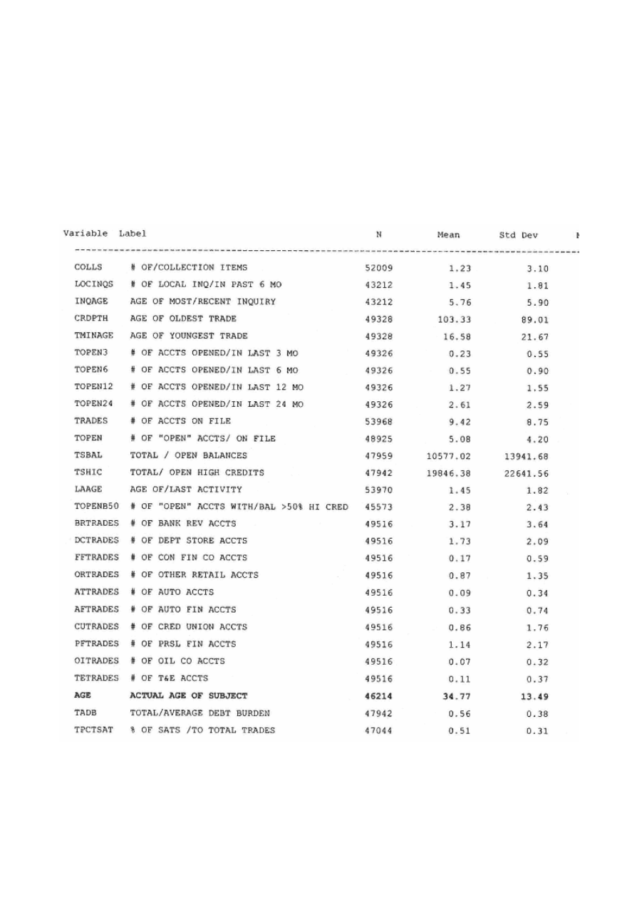
At this point, the only problem I see is with the variable age. The minimum age does not seem correct because we have no customers under the age of
18. In Figure 10.3, the univariate analysis of age shows that less than 1% of the values for age are below 18, so I will treat any value of
missing.

As I said, I am going to do things a bit differently this time to speed the processing. I have decided that because the number of missing values for each
variable is relatively small, I am going to use mean substitution to replace the values. Before I replace the missing values with the mean, I want to create
a set of duplicate variables. This allows me to keep the original values intact.

To streamline the code, I use an array to create a set of duplicate variables. An array is a handy SAS option that allows you to assign a name to a group
of variables. Each of the 61 variables is duplicated with the variable names rvar1, rvar2, rvar3, though rvar61. This allows me to perform the same
calculations on every variable just by naming the array . In fact, I am going to use several

Figure

10.2

Means

selected

variables.

Figure

10.3

Univariate

analysis

age.

arrays. This will make it much easier to follow the code because I won't get bogged down in variable names.

In the following data step, I create an array called riskvars. This represents the 61 variables that I've selected as preliminary candidates. I also create
an array called rvar. This represents the group of renamed variables, rvar1–rvar61. The "do loop" following the array names takes each of the 61
variables and renames it to rvar1-rvar61.

data riskmean;
set ch10.telco;
array riskvars (61)
COLLS LOCINQS INQAGE . . . . . . . . . . TADB25 TUTRADES TLTRADES ;
array rvar (61) rvar1-rvar61;
do count = 1 to 61;
rvar(count) = riskvars(count);
end;
run;

Page 239

NOTE: An array is active only during the data step and must be declared by name for each new data step.

The next step calculates the means for each of the 61 variables and creates an output data set called outmns with the
mean values mrvar1-mrvar61.

proc summary data=riskmean;
weight smp_wgt;
var rvar1-rvar61;
output out=outmns mean = mrvar1-mrvar61;
run;

In this next data step, I append the mean values from outmns to each record in my original data set ch10.telco. Next, I
assign the same array name, rvars, to rvars1–rvars61 . I also assign two more arrays: mrvars represents the means for
each variable; and rvarmiss indicates (0/1) if a customer has a missing value for each variable. The "do loop" creates the
variables in the array, rvarmiss, represented by rvarm1-rvarm6. These are variables with the value 0/1 to indicate which
customers had missing values for each variable. Then it assigns each mean value in the array, mrvars, to replace each
missing value for rvar1 –rvar61. The last line in the data step replaces the values for age, rvar44, that are below 18 with
the mean for age, mrvar44:

data ch10.telco;
set ch10.telco;
if (_n_ eq 1) then set outmns;
retain mrvar1 -mrvar61;

array rvars (61) rvar1-rvar61;
array mrvars (61) mrvar1 -mrvar61;
array rvarmiss (61) rvarm1-rvarm61;
do count = 1 to 61;
rvarmiss(count) = (rvars(count) = .);
if rvars(count) = . then rvars(count) = mrvars
(count);
end;
if rvar44 < 18 then rvar44 = mrvar44; /* Age */
run;

The next step finds the best transformation for each continuous variable. The steps are the same as I demonstrated in part
2, chapter 4. I now have variables with the names rvar1 –rvar61. I can use a macro to completely automate the
transformation process. I use a macro "do loop" to begin the processing. The first step uses PROC UNIVARIATE to
calculate the decile values. The next data step appends those values to the original data set, ch10.telco, and creates
indicator (0/1) variables, v1_10 – v61_10, v1_20 – v61_20,

. v1_90 – v61_90 to indicate whether the value is above or

below each decile value. The final

Page 240

portion of the data step takes each of the 61 variables through the whole set of possible transformations:

%macro cont;
%do i = 1 %to 61;

title "Evaluation of var&i";
proc univariate data=ch10.telco noprint;
weight smp_wgt;
var rvar&i;
output out=svardata pctlpts= 10 20 30 40 50 60 70 80 90 pctlpre=svar;
run;

data freqs&i;
set ch10.telco(keep= smp_wgt highrisk rvar&i rvarm&i obsnum);
if (_n_ eq 1) then set svardata;
retain svar10 svar20 svar30 svar40 svar50 svar60 svar70 svar80 svar90;
v&i._10 = (rvar&i < svar10);
v&i._20 = (rvar&i < svar20);
v&i._30 = (rvar&i < svar30);
v&i._40 = (rvar&i < svar40);
v&i._50 = (rvar&i < svar50);
v&i._60 = (rvar&i < svar60);
v&i._70 = (rvar&i < svar70);
v&i._80 = (rvar&i < svar80);
v&i._90 = (rvar&i < svar90);

v&i._sq = rvar&i**2; /* squared */
v&i._cu = rvar&i**3; /* cube root */
v&i._sqrt = sqrt(rvar&i); /* square root */
| | | | | |
| | | | | |
v&i._cosi = 1/max(.0001,cos(rvar&i)); /* cosine inverse */
run

While we're still in the macro, a logistic regression is used to select the best-fitting variables. I use maxstep=3 because
the missing indicator variables, rvarm1-rvarm61, may turn out to be predictive for many variables. And I know that
groups of variables have the exact same customers with missing values. For certain groups of variables, the missing
value indicator variable will be redundant.

proc logistic data=freqs&i descending;
weight smp_wgt;
model highrisk = v&i._10 v&i._20 v&i._30 v&i._40 v&i._50 v&i._60 v&i._70
v&i._80 v&i._90 rvar&i rvarm&i v&i._sq v&i._cu v&i._sqrt v&i._curt
v&i._log v&i._tan v&i._sin v&i._cos v&i._inv v&i._sqi v&i._cui v&i._sqri
v&i._curi v&i._logi v&i._tani v&i._sini v&i._cosi
/ selection = stepwise maxstep=3;
title "Logistic for var&i";
run;

Page 241

The final step sorts the data so that it can be remerged after the final candidate variables are selected.

proc sort data=freqs&i;
by obsnum;
run;
%end;
%mend;
%cont;

At this point, I have 61 logistic regression outputs from which to select the final variables. Table 10.2 displays the
winning transformation for each variable. Notice how many have the missing identifier as a strong predictor.

To avoid selecting a missing value indicator that will be redundant for several variables, I run a means on the 61 missing
indicator variables, rvarm1–rvarm61, and look for similar means. In Figure 10.4, notice how adjacent variables have
similar means rates. This implies that they probably matched to the same customers.

After the top two transformations are selected for each of the 61 variables, the data sets are merged back to the original
data set, ch10.telco, to create a modeling data set ch10, telco2. Finally, an indicator variable called male is created from
the lone categorical variable, gender.

Table 10.2

Final List of Candidate Variables

RVAR

DESCRIPTION

TRANS 1

TRANS 2

TRANS 3

# of collection items

v1_curt

v1_70

rvarm1

# local inq/last 6 mos

rvarm2

v2_sq

v2_cu

age of most recent inquiry

rvarm3

v3_tani

v3_cu

age of oldest trade

rvarm4

v4_curt

v4_60

age of youngest trade

rvarm5

v5_sqrt

v5_70

# accts open in last 3 mos

rvarm6

v6_sqrt

# accts open in last 6 mos

rvarm7

v7_curt

# accts open in last 12 mos

rvarm8

v8_curt

v8_cos

# accts open in last 324 mos

rvarm9

v9_curt

v9_60

# of accts on file

v10_curt

v10_90

v10_40

continues

Page 242

(Continued)

RVAR

DESCRIPTION

TRANS 1

TRANS 2

TRANS 3

# of open accts on file

rvarm11

v11_curt

v11_30

total open balances

rvarm12

v12_curt

v12_tan

total open high credits

rvarm13

v13_curt

rvar13

age of last activity

v14_logi

v14_80

rvar14

# accts with past due bal

v15_70

v15_80

amount of past due balances

rvarm16

v16_curt

v16_log

# of accts currently satisfactory

rvarm17

v17_log

v17_10

# of accts currently 30 days

rvarm18

v18_sini

# of accts currently 60 days

rvarm19

v19_sini

# of accts currently 90+ days

v20_sini

rvarm20

v20_90

# of accts currently bad debt

v21_70

rvarm21

v21_90

# of accts piad satisfactorily

vrvarm22

v22_log

v22_10

# of accts 30 days late

rvarm23

v23_sin

v23_cosi

# of accts 60 days late

rvarm24

v24_tani

# of accts 90+ days late

v25_90

rvarm25

v25_sqri

# of accts bad debt

v26_70

rvarm26

v26_90

# of accts sat in past 24 mos

rvarm27

v27_curt

v27_logi

# of accts 30 days in past 24 mos

v28_70

rvarm28

v28_cos

# of accts 60 days in past 24 mos

v29_80

rvarm29

v29_cosi

total # of open accts with bal > 0

v30_30

rvarm30

v30_logi

average number of months open

v31_70

rvarm31

v31_log

# of open accts w/bal > 75% utilization

v32_30

v32_80

rvarm32

# of open accts w/bal > 50% utilization

v33_20

rvarm33

v33_sini

# of bank revolving accts

v34_curt

rvarm34

v34_sq

# of dept store accts

rvarm35

v35_curt

v35_cosi

# of con finance co accts

rvarm36

rvar36

# of other retail accts

rvarm37

v37_curt

v37_90

(table continued on next page)

Page 243

(table continued from previous page)

RVAR

DESCRIPTION

TRANS 1

TRANS 2

TRANS 3

# of auto accts

rvarm38

# of auto finance accts

rvarm39

v39_tan

v39_cos

# of credit union accts

rvarm40

v40_log

v40_tani

# of personal fin accts

rvarm41

# of oil co accts

rvarm42

v42_sqrt

# of t&e accts

rvarm43

v43_sin

actual age of customer

v44_10

rvarm44

v44_90

total average debt burden

rvarm45

v45_90

v45_cos

% of satisfactories to total trades

rvarm46

v46_curt v46_90

# of 90+ bad debt accts in 24 mos

v47_70

v47_80

v47_90

% of all accts that are open

rvarm48

v48_cui

v48_90

# of 90-120 bad debt/pub rec derog in 24 mos

v49_log

v49_70

v49_sini

# of bad debt/pub rec derog w/i 24 mos

v50_70

v50_log

# of accts curr sat with bal > $0

rvarm51

v51_log

v51_logi

months open for all trades

rvarm52

v52_log

v52_curi

# of open trades inc/closed narratives

rvarm53

v53_sqri

v53_10

% of open trades in 24 mos to tot open trades

rvarm54

v54_tani

v54_80

% of open accts open in last 12 months

rvarm55

v55_tani

v55_sin

% of open accts open in last 6 months

rvarm56

v56_tani

v56_sin

% of open accts open in last 3 months

rvar57

rvarm57

v57_tani

# of inq in last 12 mos

rvarm58

rvar58

v58_cos

# of trades with bal < 25% utilization

rvarm59

v59_curt

v59_50

number of telco/utility accts

rvarm60

rvar60

v60_cos

number of telco accts

rvarm61

v61_cu

Figure

10.4

Similar

mean

values.

data ch10.telco2;
merge ch10.telco(keep=obsnum gender highrisk smp_wgt)
freqs1(keep=obsnum v1_curt v1_70)
freqs2(keep=obsnum rvarm2 v2_sq)
| | | | | | | |
| | | | | | | |
freqs59(keep=obsnum rvarm59 v59_curt)
freqs60(keep=obsnum rvarm60 rvar60)
freqs61(keep=obsnum rvarm61 v61_cu)
;
by obsnum;
male = (gender = 'M');
run;

I now have a data set that contains all the candidate variables. The next step is to process the model.

Processing the Model

I again use PROC CONTENTS with the short option to create a list of all the variables. I cut and paste the results into my logistic code. As in every
previous model, the first step is to split the population into a model and development sample. Recall that this is done using a weight with half missing
values. This will force the modeling process to ignore the records with weight = . (missing).

proc contents data=ch10.telco2 short;
run;

data ch10.telco2;

Team-Fly

Page 245

set ch10.telco2;
if ranuni(5555) < .5 then splitwgt = 1;
else splitwgt = .;
modwgt = splitwgt*smp_wgt;
records=1;
run;

The nest step is to run all 61 variables through a backward logistic and a stepwise logistic regression. The combination
of winning variables is run through the score selection process.

proc logistic data=ch10.telco2(keep=modwgt splitwgt smp_wgt highrisk
MALE RVAR13 . . . . . V61_CU V6_SQRT V7_CURT V8_CURT V9_CURT)
descending;
weight modwgt;
model highrisk =
MALE RVAR13 . . . . . V61_CU V6_SQRT V7_CURT V8_CURT V9_CURT
/selection=backward;
run;

proc logistic data=ch10.telco2(keep=modwgt splitwgt smp_wgt highrisk
MALE RVAR13 . . . . .V61_CU V6_SQRT V7_CURT V8_CURT V9_CURT)
descending;
weight modwgt;
model highrisk =
MALE RVAR13 . . . . . V61_CU V6_SQRT V7_CURT V8_CURT V9_CURT
/selection=stepwise;
run;

proc logistic data=ch10.telco2(keep=modwgt splitwgt smp_wgt highrisk
MALE RVAR13 . . . V61_CU V9_CURT)
descending;
weight modwgt;
model highrisk = MALE RVAR13 RVAR36 RVAR58 RVARM11 RVARM21 RVARM27
RVARM33 RVARM34 RVARM51 RVARM59 V10_CURT V12_CURT V12_TAN V15_70 V15_80
V1_CURT V20_SINI V22_LOG V25_90 V25_SQRI V32_30 V34_CURT V40_LOG V44_10
V45_90 V48_CUI V49_LOG V50_70 V52_LOG V53_10 V53_SQRI V54_TANI V56_SIN
V58_COS V59_CURT V61_CU V9_CURT
/selection=score best=1;

Figure 10.5 displays a portion of the output from the logistic regression with the score selection process. To select the
final model, I run a logistic regression with 35 variables and produce a gains table. I then select a 20 variable model and
repeat the process. The difference is so minimal that I decide to stick with the 20-variable model.

The following code is used to produce the final model. The keep= statement in the first line is used to reduce the number
of variables that are brought into the processing. This allows the program to run much faster. While only half the

Figure

10.5

Score

logistic

regression.

customers were used in processing, the out=ch10.scored data set contains all the customers. This is the advantage of using missing values for half the
weights. Every record is scored with the final predictive value. I use the (where=(splitwgt=.)) option to allow validation on those customers not used
to build the model:

proc logistic data=ch10.telco2(keep= records modwgt splitwgt smp_wgt
highrisk MALE RVAR58 RVARM21 RVARM34 RVARM51 V10_CURT V12_TAN V15_70
V1_CURT V20_SINI V22_LOG V25_90 V34_CURT V44_10 V45_90 V53_SQRI V54_TANI
V58_COS V61_CU V9_CURT) descending;
weight modwgt;
model highrisk = MALE RVAR58 RVARM21 RVARM34 RVARM51 V10_CURT V12_TAN
V15_70 V1_CURT V20_SINI V22_LOG V25_90 V34_CURT V44_10 V45_90 V53_SQRI
V54_TANI V58_COS V61_CU V9_CURT;
output out=ch10.scored(where=(splitwgt=.)) p=pred;
run;
proc sort data=ch10.scored;
by descending pred;
run;

Page 247

The remaining code creates the deciles and produces the gains table.

proc univariate data=ch10.scored noprint;
weight smp_wgt;
var pred;
output out=preddata sumwgt=sumwgt;
run;

data ch10.scored;
set ch10.scored;
if (_n_ eq 1) then set preddata;
retain sumwgt;
number+smp_wgt;
if number < .1*sumwgt then val_dec = 0; else
if number < .2*sumwgt then val_dec = 1; else
if number < .3*sumwgt then val_dec = 2; else
if number < .4*sumwgt then val_dec = 3; else
if number < .5*sumwgt then val_dec = 4; else
if number < .6*sumwgt then val_dec = 5; else
if number < .7*sumwgt then val_dec = 6; else
if number < .8*sumwgt then val_dec = 7; else
if number < .9*sumwgt then val_dec = 8; else
val_dec = 9;
run;

proc tabulate data=ch10.scored;
weight smp_wgt;
class val_dec;
var highrisk pred records;
table val_dec='Decile' all='Total',
records='Customers'*sum=' '*f=comma11.
pred='Predicted Probability'*mean=' '*f=11.5
highrisk='Percent Highrisk'*mean=' '*f=11.5
/rts = 9 row=float;
run;

The parameter estimates and model statistics are displayed in Figure 10.6. Notice the variable with the highest Wald chi-
square value is v1_curt. Looking back at Table 10.2, we see that this is a function of the number of collection items. This
is the strongest predictor when considered in combination with all other predictors.

The decile analysis in Figure 10.7 shows both strong rank ordering and good predictive power. The next step is to
validate the final model.

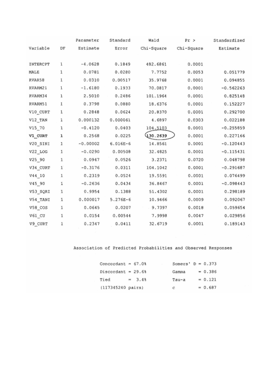
Figure

10.6

Final

model

output.

Validating the Model

Recall that in the beginning of the chapter, I said that in addition to the 300+ predictive variables, I also purchased a generic risk score
from the credit bureau. To validate my model scores, I compare the rank ordering ability of my score to that of the generic score. Figure
10.8 compares the actual percentages in the best deciles. Also the lift is superior for the model I developed. This can also be seen in the
gains chart in Figure 10.9. It is not unusual to do better with your own data. The real test will be in the implementation.

To complete the validation process, I will calculate bootstrap estimates for my predictive model.

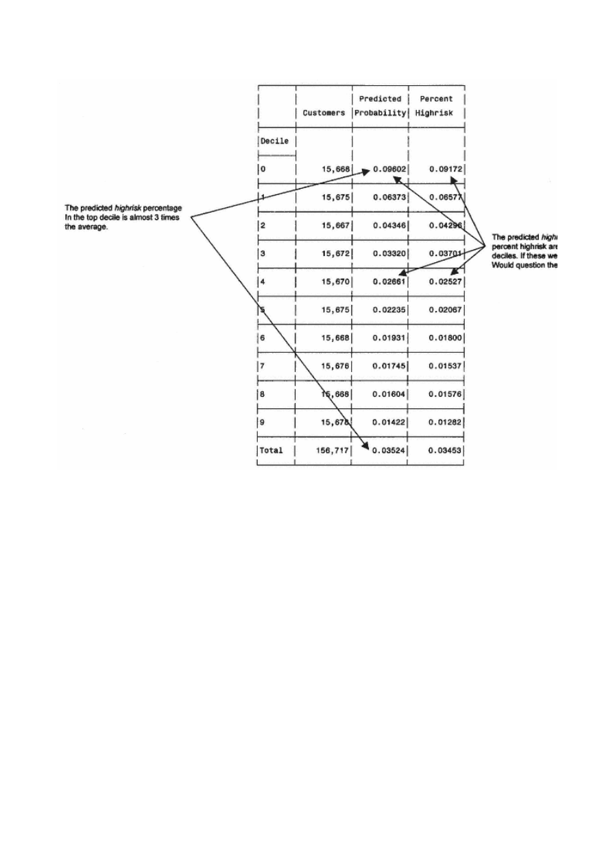
Figure

10.7

Validation

decile

analysis.

Bootstrapping

The program for creating the bootstrap estimates is similar to the program in chapter 9. The main difference is that in chapter 9, I had three
variables, response, 12-month sales, and lift for 12 -month sales. Here I want two bootstrap estimates: predicted value (pred
(bsest_h) and the lift (bsest_l) for highrisk. The following represents the final stage of the bootstrap program. This tabulate code creates the
output in Figure 10.10.

proc tabulate data=ch10.bs_sum;
weight smp_wgt;
var liftf bsest_h hrmnf lci_h uci_h bsest_l lftmbs lci_l uci_l;
class val_dec;
table (val_dec='Decile' all='Total'),
(hrmnf='Predicted High Risk'*mean=' '*f=percent6.
bsest_h='BS Est High Risk'*mean=' '*f=percent6.
lci_h ='BS Lower CI Resp'*mean=' '*f=percent6.
uci_h ='BS Upper CI Resp'*mean=' '*f=percent6.
liftf ='High Risk Lift'*mean=' '*f=6.
bsest_l='BS Est Lift'*mean=' '*f=6.
lci_l ='BS Lower CI Lift'*mean=' '*f=6.
uci_l ='BS Upper CI Lift'*mean=' '*f=6.)
/rts=10 row=float;
run;

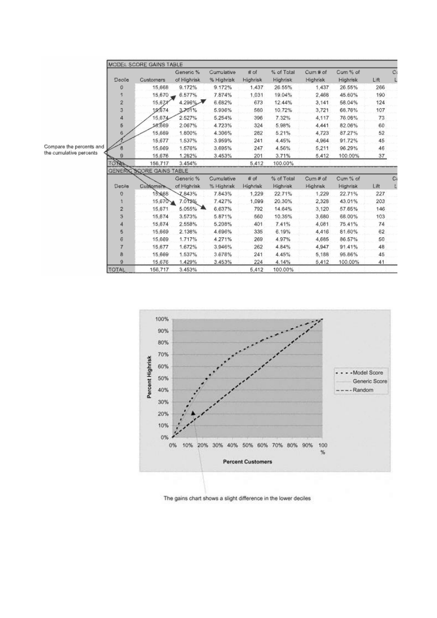
Figure

10.8

Comparison

model

score

generic

score.

Figure

10.9

Gains

chart

for

score

comparison.

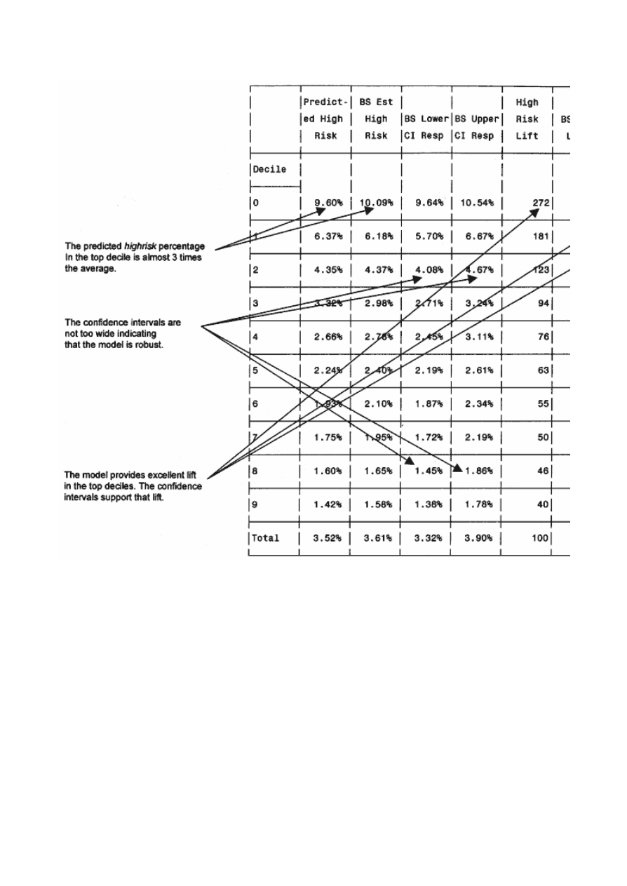
Figure

10.10

Model

score

bootstrap

estimates

and

confidence

intervals.

The overall model performance validates well with the top decile capturing almost three times the average. The tight width of the confidence intervals
shows that the model is robust.

Implementing the Model

Risk scores are used in many phases of customer relationship management. As we saw in part 2, a risk adjustment was used to determine the lifetime
value of prospects. This was based on a three-way matrix of gender, age, and marital status. It easily could have been derived from a risk model. In
chapter 8, we saw how risk scores are used to segment customers and prospects. The model we just completed is being used to score First Reserve's
banking customer for Eastern Telecom. Those banking customers who are low risk will receive a great offer for cellular products and services in their
next monthly statement.

Page 252

Scaling the Risk Score

To make risk comparison more user friendly, most risk scores are translated into a scale ranging from 450 to 850. This is
accomplished by selecting a base value that equates to a 50/50 chance of some negative risk action, i.e., your objective.
The scale is designed in such a way that the risk decreases as the score increases— the highest scoring customers are the
lowest risk.

For the case study, I want to derive a formula to translate the probability of highrisk to a number between 450 and 850.
Let's say I want to base the score at 480. The base equates to a probability of default of 50% or an odds of 50/50.
Because the parameter estimates in logistic regression are linear in the log of the odds, the output can simply be rescaled
so any desired number of score points doubles the odds. For example, the formula below doubles the odds every 40
points:

Score = 480 + 57.706 * log((1 – p)/p)

Notice that I use (1-p)/p because I want ''good to bad" odds for this formula. Table 10.3 shows the levels of probability
along with the steps to translate it into the scaled risk score.

For Eastern Telco, the following code translates the predicted values into scores and creates the table in Figure 10.11:

data ch10.scored;
set ch10.scored;
riskscor = 480 + 57.706*(log((1-pred)/pred));
run;

proc format;
value score
450-<500 = '450 - 500'
500-<550 = '500 - 550'
550-<600 = '550 - 600'
600-<650 = '600 - 650'
650-<700 = '650 - 700'
700-<750 = '700 - 750'
;
run;

proc tabulate;
weight smp_wgt;
format riskscor score.;
class riskscor;
var pred records;
table riskscor=' ' all='Total',
(records='Customers'*sum=' '*f=comma12.
pred='Predicted Probability'*mean=' '*f=percent12.2)

Page 253

Table 10.3

Relationship of Odds to Scaled Risk Scores

PROBABILITY
OF
BAD

GOOD

BAD ODDS

LOG

ODDS

DERIVED

RISK

SCORE

50.00%

1/1

0.000

480

33.33%

2/1

0.693

520

26.12%

2.83/1

1.040

540

20.00%

4/1

1.386

560

15.02%

5.66/1

1.733

580

11.11%

8/1

2.079

600

8.12%

11.32/1

2.426

620

5.88%

16/1

2.773

640

4.23%

22.64/1

3.120

660

3.03%

32/1

3.466

680

2.16%

45.26/1

3.813

700

1.54%

64/1

4.161

720

1.09%

90.74/1

4.508

740

0.78%

128/1

4.846

760

0.55%

180.82/1

5.197

780

0.39%

256/1

5.545

800

/rts=20 row=float box='Risk Score';
run;

Figure 10.11 depicts good news for Eastern Telco. Most of First Reserve's customers have a relatively low risk level. If
Eastern selects all names with a score of 650 or above, it will have almost 125,000 low-risk First Reserve customers to
solicit.

A Different Kind of Risk:
Fraud

The main focus of this chapter has been on predicting risk for default on a payment. And the methodology translates
very well to predicting the risk of claims for insurance. There is another type of risk that also erodes profits: the risk of
fraud. Losses due to fraud cost companies and ultimately consumers millions of dollars a year. And the threat is
increasing as more and more consumers use credit cards, telecommunications, and the Internet for personal and business
transactions.

Team-Fly

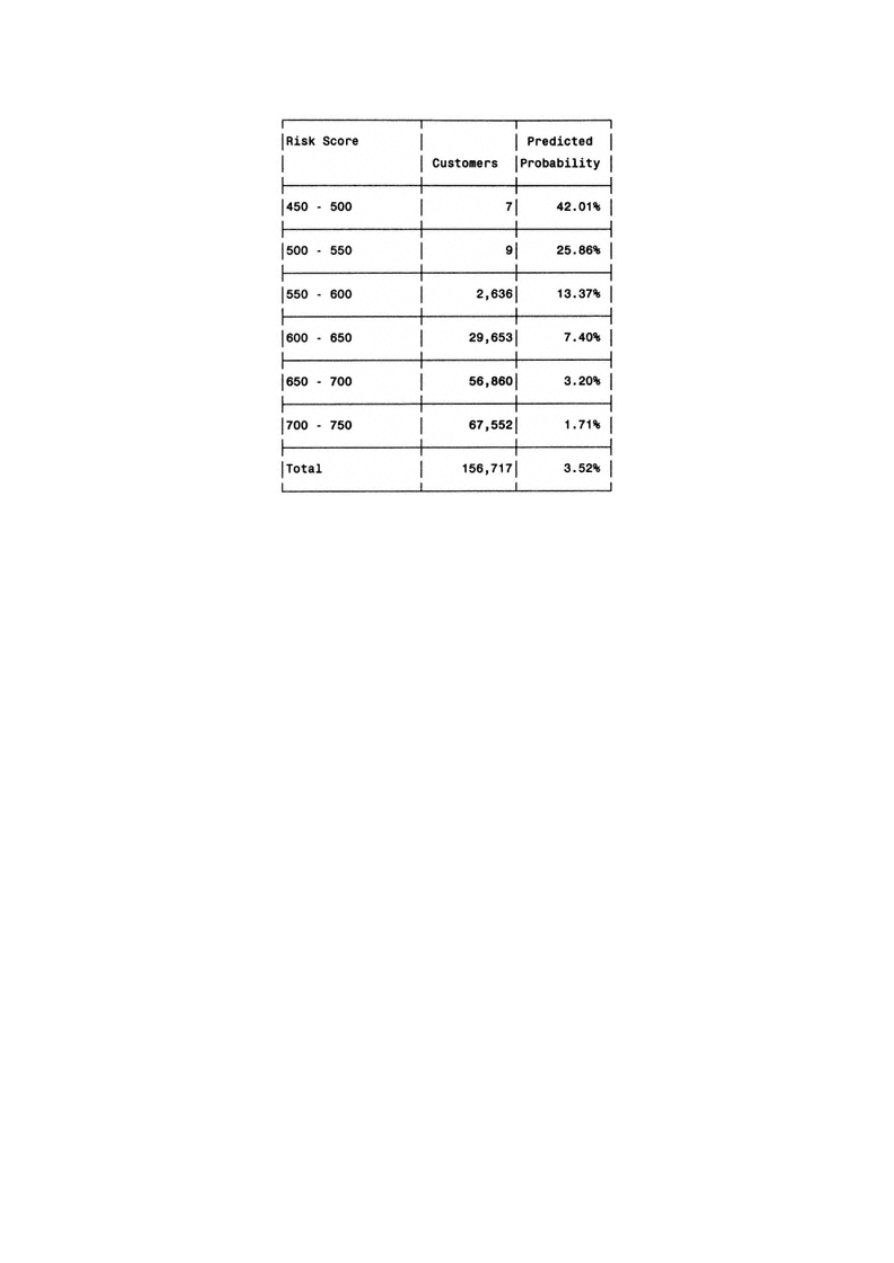
Page 254

Figure

10.11

Tabulation

risk

scores.

Jaya Kolhatkar, Director of Fraud Management for Amazon.com, discusses the mechanics of developing fraud models
and the importance of proper implementation:

Fraud in the e-tailing world has increased rapidly over the past two years. Being a virtual marketplace, most of the fraud
checks in the physical retail world do not apply. Primarily, fraud is committed through the use of credit cards. There are
several effective fraud management tools available from the credit card associations like address verification system, fraud
scores, etc.; however, these are not enough for a rigorous fraud management system.

As Amazon.com moved from selling just books to books, music, video, consumer electronics, etc., fraud losses increased.
In order to control these losses a two-pronged approach was developed. The two components were data analysis/model
building and operations/investigations.

The data analysis component is the backbone of the fraud system. It is important to underscore that because fraud rates
within the population are so low, a blend of two or more modeling techniques seems to work best at isolating fraud orders
within the smallest percentage of the population. We have used logistic regression, decision trees, etc., in combination to
create effective fraud models. Low fraud rates also impact data preparation/analysis. It is easy to misjudge spurious data for
a new fraud trend.

Page 255

Another important issue to keep in mind at this stage of model development is model implementation. Because we function
in a real-time environment and cannot allow the scoring process to be a bottleneck in our order fulfillment process, we need
to be very parsimonious in our data selection. While, at first, this seems to be very limiting from a variable selection point
of view, we have found that using a series of scorecards built on progressively larger set of variables and implemented on a
progressively smaller populations is very effective.

Given the "customer-centric" philosophy of Amazon.com, no order (except perhaps the most blatant fraud order) is
cancelled without manual intervention. Even the best predictive system is inherently prone to misclassification. We use data
analysis and optimization techniques to help the investigations staff hone in on the right set of orders.

To be effective in reducing fraud losses over a long period of time, the fraud models need to be constantly updated to
capture any new patterns in fraud behavior.

Summary

Did you notice a lot of similarities between the risk modeling process and the response modeling process? While the
goals and company focus are very different, the mechanics are quite similar. Sure, there were a few variations in the use
of weights and the streamlined variable processing, but the main goal was achieved. We were able to determine which
characteristics or variables are best at identifying risky customers.

This methodology works well for any industry seeking to limit risk. If you've ordered a new Internet service, the
company probably looked at your credit report. They may have even evaluated your application based on a risk score
similar to the one we just developed. The same methodology works well to predict the risk of claims. You would
substitute claims data for risk data and gather predictive variables from the customer database and overlay data.

I hope you're not too stuffed. We have a couple more recipes to go. In the next chapter, I demonstrate how to build a
churn model. Bon appetit!

Page 257

Chapter 11—
Retaining Profitable Customers:
Modeling Churn

Have you ever been interrupted by a phone call during dinner with an invitation to switch your long-distance service? Or
how about those low-rate balance transfer credit card offers that keep filling your mailbox? Many companies are finding
it harder and harder to attract new customers. As a result, the cost of acquiring new customers is on the rise. This has
created a major shift in marketing. Many companies are focusing more on retention because it costs much less to keep a
current customer than to acquire a new one. And one way to improve retention is to take action before the customer
churns. That's where churn models can help!

Churn models, also known as retention or attrition models, predict the probability of customer attrition. Because attrition
has such a powerful impact on profitability, many companies are making these models the main focus of their customer
loyalty program. In this chapter, I begin with a discussion of the importance of customer loyalty and its effect on profits
in a number of industries. The remainder of the chapter details the development of a churn model that predicts the effect
of a rate increase on credit card balances. The steps are familiar. I begin by defining the objective. Then I prepare the
variables, process the model, and validate. I wrap up the chapter with some options for implementing a churn model and
the effect on overall customer profitability.

Page 258

Customer Loyalty

As I just mentioned, the main advantage of a retention program is economics. If you have $1 to spend on marketing, you
would be much better off spending it on customer retention than customer acquisition. Why? It's much more expensive
to attract a new customer than to retain a current one. Also, loyal customers tend to be less price-sensitive.

The airline industry is very adept at building customer loyalty. The more you fly with one airline, the more benefits you
receive. Many other industries have followed the pattern with loyalty cards and incentives for repeat business. The
gambling industry has embraced customer profiling and target modeling to identify and provide benefits for their most
profitable customers. Credit card banks have affinity cards with everything from schools to pet clubs. These added
benefits and incentives are essential for survival since most companies are learning that it is difficult to survive by
competing on price alone. Building customer loyalty by creating additional value is becoming the norm in many
industries.

Defining the Objective

For many industries, defining the objective is simple. You can have only one long-distance provider. If you switch, it's a
complete gain for one company and a complete loss for the other. This is also true for energy providers; you have one
source for your electrical power. Insurance customers generally patronize one company for certain types, if not all, of
their insurance. For some industries, though, it's not so simple. For example, a catalog company may hope you are a
loyal customer, but it doesn't really know what you are spending with its competitors. This is true for most retailers.

Credit card banks have exceptional challenges in this area due to the combination of stiff competition and industry
dynamics. For the most part, the only profitable customers are the "revolvers" or those customers that carry a balance.
"Silent attrition" occurs when customers pay down their balances without closing their accounts. Pure transactors, or
customers that pay their balance every month, are profitable only if their monthly purchases are above a certain amount.

This chapter's recipe details the steps for building a model to predict attrition or churn for credit card customers
following a rate increase. Rowan Royal Bank has a modest portfolio of 1.2 million customers. Its interest rates or APRs
(annual percentage rates) are lower than the industry average, especially on its

Page 259

high-risk customers. But before it increases rates on the entire group of high-risk customers, the bank wants to predict
which customers are highly rate-sensitive. In other words, they want to determine which customers have a high
probability of shifting balances away following a rate increase. For these customers, the increase in interest revenue may
be offset by losses due to balances attrition.

By definition, the opposite of customer retention or loyalty is customer attrition or churn. Measuring attrition is easy.
Defining an attritor is the challenging part. There are many factors to consider. For example, how many months do you
want to consider? Or do you compare lost balances to a beginning balance in a given month or the average of several
months? Do you take a straight percentage drop in balances? If so, is this meaningful for someone with a very low
beginning balance? In other words, the definition should not just describe some arbitrary action that ensures a strong
model. The definition should be actionable and meaningful to the business goals. See the accompanying sidebar for
Shree Pragada's discussion on the significance of this definition.

Defining Attrition to Optimize Profits

Shree Pragada, Vice President of Customer Acquisition at Fleet Credit Card Bank, discusses the effect of the
definition of attritors on profitability.

The emphasis in model development is usually just on the model performance measures and not much on the model
usage. In addition to building a statistically sound model, an analyst should focus on the business application of the
model.

The following is an example from the financial services industry. A business manager requests for a model to
identify balance attritors. If the analyst were to build a model just to suffice the request, he or she would define the
objective to identify just balance attritors. But further inquiry into the application of the model reveals that the
attrition probabilities will be applied to customers' account balances to estimate the level of balance at attrition
risk— and eventually in a customer profitability system for targeting for a marketing promotion. The analyst would
now change the objective to predicting balance attritors with the emphasis on attritors with significant account
balances. As the financial impact of attrition is the final goal, such a change in the definition of the dependent
variable will improve the effectiveness of the model in the business strategies.

The logical choice in this modeling exercise was to build a logistic model to predict the likelihood of attrition. The
exercise also involved comparing several definitions of the dependent variable. For simplicity, we will focus on
only two dependent variable definitions— one with the balance cut -off and the other without.

Definition: % Reprice Balance Attrition, the dependent variable, is the percent reduction in balance:

% Balance Attrition = 1 – Fraction of Pre-Event Balances Remaining

Business analysis reveals that most accounts tend to be unprofitable when more than 75% of the pre-reprice balances were paid off.
Therefore, a binary variable is defined using this 75% balance attrition cutoff:

Dependent Variable: = 1 If % of Balance Attrition GT 75% = 0 otherwise

Fraction of balances left is defined as Average of the Three-Month Balances Post-Event over Average Annual Balance Pre

As the goal of this model is to predict the probability of "balance" attrition, the definition of the dependent variable has been altered to
focus on the magnitude (or dollar amount) of balance attrition in addition to the likelihood of attrition. By doing this, customers with a
high percent of attrition but with marginal amount of balance attrition (dollar amount) will be treated as nonattritors. As a result we
can be more confident that we are modeling deliberate and significant balance attrition and not just swings in balance level that may
not be related to reprice. The modified definition is:

Dependent Variable: = 1 If % of Balance Attrition GT 75% and Dollar Amount GT $1,000 = 0 Otherwise

Table 11.1 summarizes the model measurement statistics and percent of attritors in the top 10 of 20 segments of the Cumulative Gains
tables:

Table 11.1 Comparison of Dependent Variable Definition–Minimum Percentage

MODEL
DESCRIPTION

# / % OF ACCOUNTS
CATEGORIZED AS
ATTRITORS OF THE
TOTAL SAMPLE OF
53,877 A/CS

RANK OF MAX.
SEPARATION (OF
20)

CLASSIFICATION
@ MAX.
SEPARATION

% OF ACCOUNT
SEPARATED IN THE
TOP 50% OF THE
POP

(1) Dependent
Variable
Definition with
a $1,000 Cut-off

12,231 / 22%

35.0%

70.49%

75%

(1) Dependent
Variable
Definition without
$1,000 Cut-off

15,438 / 29%

39.9%

72.47%

76%

To the surprise of the Implementation/Targeting groups, Model 1 was recommended despite its lesser strength in identifying
attritors. Because the model is used to understand the financial impact as a result of attrition, the dependent variable in Model 1 was
changed to focus on attritors with significant account balances (over $1,000 in this case). This lowered the ability of the model to
identify the likelihood of attrition, but it significantly improved the rank ordering of attritors with significant account balances, as
evident in Table 11.2.

Table 11.2

Comparison of Dependent Variable Definition–Minimum

MODEL
DESCRIPTION

# / % OF
ACCOUNTS
CATEGORIZED
AS ATTRITORS
OF THE TOTAL
SAMPLE OF
53,877 A/CS

RANK OF
MAX.
SEPARATION
(OF 20)

CLASSIFICATION
@ MAX.
SEPARATION

% OF
ACCOUNT
SEPARATED
IN THE TOP
50% OF THE
POP

% OF TOTAL
LOST DOLLARS
SEPARATED IN
THE TOP 50%
OF THE POP

(1) Dependent Variable
Definition with a $1,000
Cut-off

12,231 / 22%

35.0%

70.49%

75%

72%

(1) Dependent Variable
Definition without $1,000
Cut-off

15,438 / 29%

39.9%

72.47%

76%

62%

The data for modeling was randomly selected from the high -risk section of Rowan Royal Bank's customer portfolio. The attrition rate
is almost 24%, so further sampling wasn't necessary. Prior work with attrition modeling had narrowed the field of eligible variables.
In fact, a couple of the variables are actually scores from other models. Figure 11.1 shows the list of variables. Note: The term
is commonly used in the credit card industry and stands for Financial Revolving Unsecured Trade .

I am defining an attritor using the definition developed by Shree Pragada in the above sidebar. The variable pre3moav equals the
average balance for the three months prior to the rate increase. The variable pst3moav equals the average balance for the three
period beginning the fourth month following the rate increase.

data ch11.rowan;
set ch11.rowan;
pre3moav = mean(prebal3,prebal2,prebal1);
pst3moav = mean(pstbal4,pstbal5,pstbal6);

dollattr = (pre3moav - pst3moav)/pre3moav;

Page 262

Figure

11.1

List

variables.

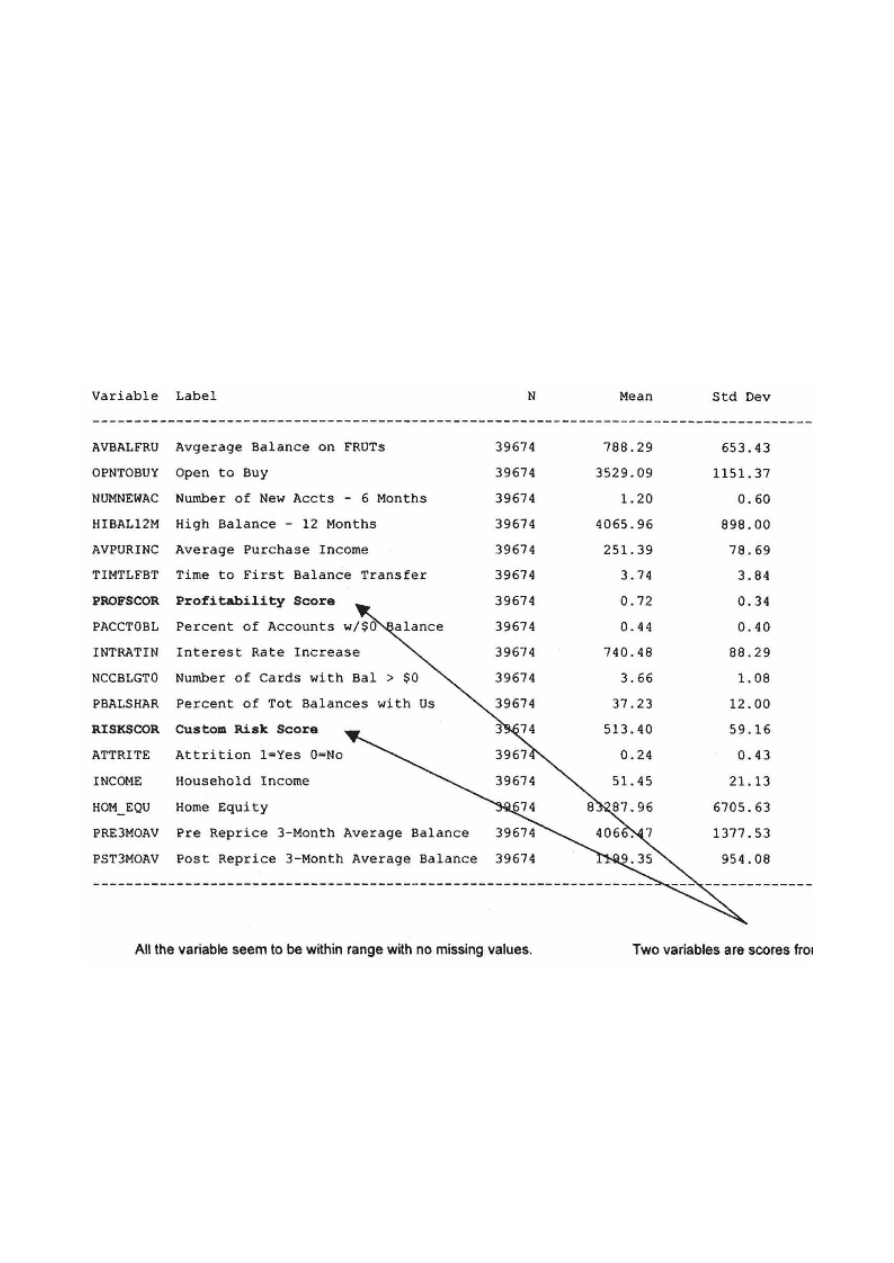
if dollattr > 1000 and dollattr/pre3moav > .75 then attrite = 1;
else attrite = 0;
run;

Preparing the Variables

This turns out to be one of the easiest recipes because I have relatively few variables. I begin by looking at the continuous variables using a program
similar to the one I used in chapter 10. I'll follow up with the categorical variables using standard frequencies.

Continuous Variables

I begin with PROC MEANS to see if the continuous variables have missing or extreme values (outliers). Figure 11.2 displays the output.

proc means data=ch11.rowan maxdec=2;
run;

Figure

11.2

Means

continuous

variables.

Page 264

All the variables seem to be within range with no missing values. The next step is to look for segmentation opportunities
and find the best form of each continuous variable. The following macro is a slight variation on the macro in chapter 10.
It processes all continuous variables (listed at the bottom of the macro). The var calls the full variable name and svar
calls a three-letter nickname for the variable used to create prefixes throughout the program. The %INCLUDE command
accesses the program that creates the transformations run the logistic regression to determine the best final variable
formations. That program is named transf:

%macro cont (var, svar);

title "Evaluation of &var";
proc univariate data=ch11.rowan noprint;
var &var;
output out=ch11.&svar.data pctlpts= 10 20 30 40 50 60 70 80 90 99 100
pctlpre=&svar;
run;

<<CODE IN THIS SECTION IS SIMILAR TO TRANSFORMATION CODE IN CHAPTER 10>>

proc freq data=&svar.dset;
table attrite*&svar.grp10/chisq;
run;

%INCLUDE transf;

%mend;
%cont(avbalfru, avb);
%cont(opntobuy, opn);
%cont(numnewac, num);
%cont(avpurinc, avp);
%cont(hibal12m, hib);
%cont(hom_equ, hom);
%cont(income, inc);
%cont(timtlfbt, tim);
%cont(nccblgt0, ncc);
%cont(pacct0bl, pac);
%cont(pbalshar, pba);
%cont(intratin, int);
%cont(riskscor, ris);
%cont(profscor, pro);

Similar to the program in chapter 10, this program automates the segmentation by creating segments at each decile. The
segment variables are binary variables that split the file at each decile. The segment variables are tested along with the
transformations in a stepwise logistic to determine the best two transformations.

Figure 11.3 shows the decile segmentation for the variable avbalfru. Notice how the attrition rate flattens out in deciles 3
through 5. This is a likely place for

Team-Fly

Page 265

Figure

11.3

Decile

segmentation

for

average

balance

FRUTs.

a binary split to create a segmentation variable. In Figure 11.4, notice how the variable avb_20 was selected as the
second best-fitting transformation.

Table 11.3 lists all the continuous variables and their top two transformations. These will be used in the final model
processing.

Categorical Variables

The following frequency calculates the attrition rate for every level of each categorical variable.

proc freq data=ch11.rowan;
table attrite*(age_lt25 autoloan child donate gender hh_ind
homeown mailord marital mortgage popdens region retired sgle_fam
somecoll ssn_ind)/ chisq missing;
run;

Figure 11.5 displays the output for population density (popdens). The attrition rates are very different for each level, so I
will create indicator variables for three of the four levels and allow the fourth level to be the default. I repeat this process
for every categorical variable. The following code transforms the categorical variables into numeric form for use in the
model.

Page 266

Figure

11.4

Logistic

output

for

average

balance

FRUTs.

data ch11.rowan;
set ch11.rowan;

city = (popdens = 'C');
suburb = (popdens = 'S');
rural = (popdens = 'R');
if gender = 'I' then gender = 'U';
west = (region in ('west', ' '));
married = (marital = 'M');
single = (marital = 'S');
unkngend = (gender = 'U');
if age_lt25 = 'Y' then age_d = 1;
else age_d = 0;
if autoloan = 'Y' then auto_d = 1;
else auto_d = 0;
if donate = 'Y' then donat_d = 1;
else donat_d = 0;

Page 267

Table 11.3

List of Continuous Variable Transformations

VARIABLE NAME

DESCRIPTION

TRANS 1

TRANS 2

avbalfru

Average Balance on FRUTs

avb_20

avb_cu

opntobuy

Open to Buy

opn_30

opn_cu

numnewac

Number of New Accts in Last 6 Months

num_sq

num_exp

avpurinc

Average Purchase Income

avp_50

avp_cu

hibal12m

High Balance in Last 12 Months

hib_20

hib_sqrt

hom_eq

Home Equity

hom_90

hom_exp

income

Income

inc_30

inc_90

timtlfbt

Time to First BT

tim_sqrt

tim_sin

nccblgt0

Number of Cards with Bal > $0

ncc_90

ncc_curi

pacctobl

Percent of Accts with $0 Balance

pac_90

pac_sini

pbalshar

Percent of Total Balances with Us

pba_10

pba_cu

intratin

Interest Rate Increase

int_20

int_sqrt

riskscor

Custom Risk Score

ris_60

ris_cui

profscor

Profitability Score

pro_60

pro_sqri

if hh_ind = 'H' then hhind_d = 1;
else hhind_d = 0;
if homeown = 'Y' then home_d = 1;
else home_d = 0;
if mailord = 'Y' then mail_d = 1;
else mail_d = 0;
if mortgage = 'Y' then mort_d = 1;
else mort_d = 0;
if retired = 'Y' then ret_d = 1;
else ret_d = 0;
if sgle_fam = 'Y' then sgle_d = 1;
else sgle_d = 0;
if somecoll = 'Y' then coll_d = 1;
else coll_d = 0;
run;

Page 268

Figure

11.5

Frequency

analysis

population

density.

Now that we have our full list of powerful candidate variables, it is time to process the full model.

Processing the Model

These steps are similar to past recipes. I begin with the backward and stepwise and throw the winners from both into a
score selection model. In this case, the results from the backward and stepwise were identical, so I took the 22 chosen
variables and ran logistic regression with the selection = score, best = 2 options. Figure 11.6 displays an excerpt of the
results. The scores change minimally, so I am going to test a couple of different model sizes to see if it makes a
difference. This is usually a worthwhile exercise if the scores are close.

The code for processing the 15-variable model is shown here:

proc logistic data=ch11.rowan(keep= modwgt records smp_wgt splitwgt
attrite AVB_CU AVPURINC AVP_50 NCCBLGT0 NCC_CURI NUMNEWAC OPNTOBUY
OPN_30 PACCT0BL PAC_90 PBALSHAR PBA_CU PROFSCOR PRO_60 TIMTLFBT)
descending;

Figure

11.6

Score

output.

weight modwgt;
model attrite =
AVB_CU AVPURINC AVP_50 NCCBLGT0 NCC_CURI NUMNEWAC OPNTOBUY OPN_30
PACCT0BL PAC_90 PBALSHAR PBA_CU PROFSCOR PRO_60 TIMTLFBT;
output out=ch11.scored(where=(splitwgt=.)) p=pred;
run;

The steps down to PROC TABULATE, are identical to those in chapter
10.

title "15 Variable Model";
proc tabulate data=ch11.scored;
weight smp_wgt;
class val_dec;

var attrite pred records;
table val_dec='Decile' all='Total',
records='Customers'*sum=' '*f=comma9.
pred='Predicted Probability'*mean=' '*f=11.5

attrite='Percent Attritors'*mean=' '*f=percent9.2
/rts = 8 row=float;
run;

This process is repeated for the 10- and 22 -variable models. The results are compared in Figure 11.7. You can see that there really isn't a
significant difference in performance, so you might select the number of variables based on other criteria such as model stability or
explanability.

Validating the Model

By now you've probably noticed that I like to calculate bootstrap estimates on all my models. It gives me the comfort that I have a robust
model that doesn't over-fit the data. But before I calculate bootstrap estimates, I am going to compare the ability of the generic attrition score,
gen_attr , to the model's ability to rank the true attriters. Figure 11.8 shows a gains table comparison of the three models and the generic score.

Figure

11.7

Model

comparison

for

number

variables.

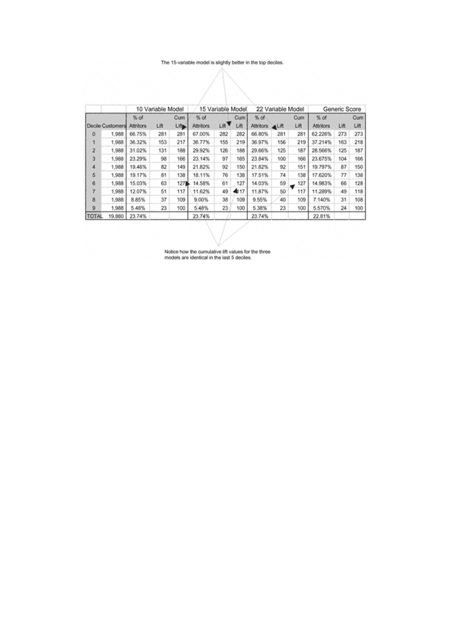
Page 271

Figure

11.8

Score

comparison

gains

table.

The differences or similarities are easy to see in Figure 11.9, which is a gains chart comparing all four model scores.
This also shows that there is hardly any difference in the performance of the three models.

Bootstrapping

The following code is excerpted from the bootstrapping macro in chapter 10. It is identical except for the dependent
variable and the variable prefixes and suffixes. Recall that the data set, ch11.scored, is an output data set from PROC
LOGISITIC, shown previously.

data ch11.scored;
set ch11.scored(keep= pred attrite splitwgt records val_dec smp_wgt);
run;

proc univariate data=ch11.scored noprint;
weight smp_wgt;
var attrite;
output out=preddata sumwgt=sumwgt mean= atmean;
run;

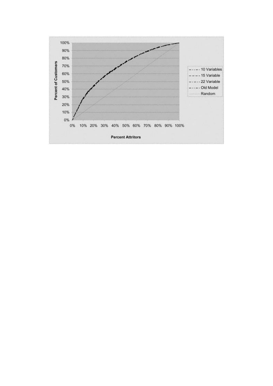
Page 272

Figure

11.9

Score

comparison

gains

chart.

proc sort data=ch11.scored;
by descending pred;
run;

data ch11.scored;
set ch11.scored;
if (_n_ eq 1) then set preddata;
retain sumwgt atmean;
run;

proc summary data=ch11.scored;
weight smp_wgt;
var pred;
class val_dec;
output out=ch11.fullmean mean=atmnf;
id smp_wgt;
run;

data atfmean(rename=(atmnf=atomn_g) drop=val_dec);
set ch11.fullmean(where=(val_dec=.) keep=atmnf val_dec);
run;

data ch11.fullmean;
set ch11.fullmean;
if (_n_ eq 1) then set atfmean;
retain atomn_g;
run;

Page 273

%macro bootst25;
%do samp = 1 %to 25;

<< THE REMAINDER OF THE CODE IN THIS SECTION IS SIMILAR TO THE BOOT-
STRAPPING CODE IN CHAPTER 6 >>

The following PROC TABULATE creates the table seen in Figure 11.10.

proc tabulate data=ch11.bs_sum;
weight smp_wgt;
var liftf bsest_a atmnf lci_a uci_a bsest_l lftmbs lci_l uci_l;
class val_dec;
table (val_dec='Decile' all='Total'),
(atmnf='Predicted Attrition'*mean=' '*f=percent10.2
bsest_a='BS Est Attritors'*mean=' '*f=percent10.2
lci_a ='BS Lower CI Resp'*mean=' '*f=percent10.2
uci_a ='BS Upper CI Resp'*mean=' '*f=percent10.2

liftf ='Actual Lift'*mean=' '*f=8.
bsest_l='BS Est Lift'*mean=' '*f=8.
lci_l ='BS Lower CI Lift'*mean=' '*f=8.
uci_l ='BS Upper CI Lift'*mean=' '*f=8.)
/rts=10 row=float;
run;

In figure 11.10, we can see the bootstrap estimates and confidence intervals for the probability of attrition or churn. The
tight range of the confidence interval give me confidence that the model is robust.

Implementing the Model

Now that we have a probability of churn, we can use it in a couple of ways. First, we can use it to gain a deeper
understanding of our customers. This is achieved through customer profiling. Using a decile analysis of churn score
across some key drivers of attrition or churn, we can begin to understand the characteristics of a loyal or disloyal
customer.

Creating Attrition Profiles

Rowan Royal Bank is interested in knowing how the key drivers of the 15-variable model behave within each decile.
With this information, it can create profiles of its customers based on their probability to move balances following a rate
increase. The following code, similar to the code used in chapter 7, used PROC TABULATE to create the gains table in
Figure 11.11.

Team-Fly

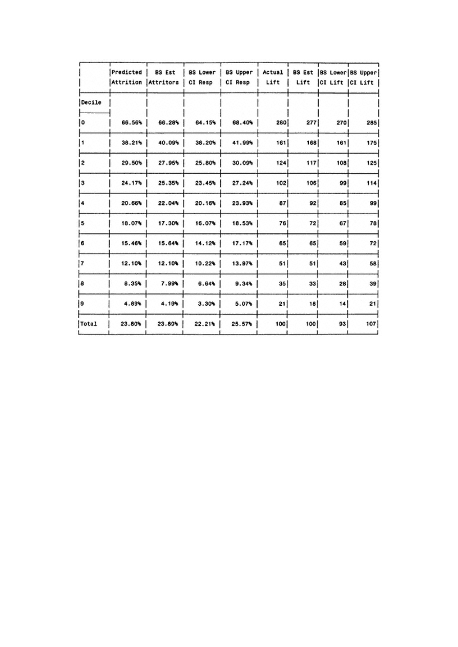
Page 274

Figure

11.10

Bootstrap

estimates

15-variable

attrition

model.

proc tabulate data=ch11.scored;
weight smp_wgt;
class val_dec ;
var AVPURINC NCCBLGT0 NUMNEWAC OPNTOBUY PACCT0BL
PBALSHAR PROFSCOR TIMTLFBT;
table val_dec=' ' all='Total',
AVPURINC*mean=' '*f=dollar8.
NCCBLGT0*mean=' '*f=comma8.
NUMNEWAC*mean=' '*f=comma8.
OPNTOBUY*mean=' '*f=dollar8.
PACCT0BL*mean=' '*f=percent8.
PBALSHAR*mean=' '*f=percent8.
PROFSCOR*mean=' '*f=8.2
TIMTLFBT*mean=' '*f=8.2

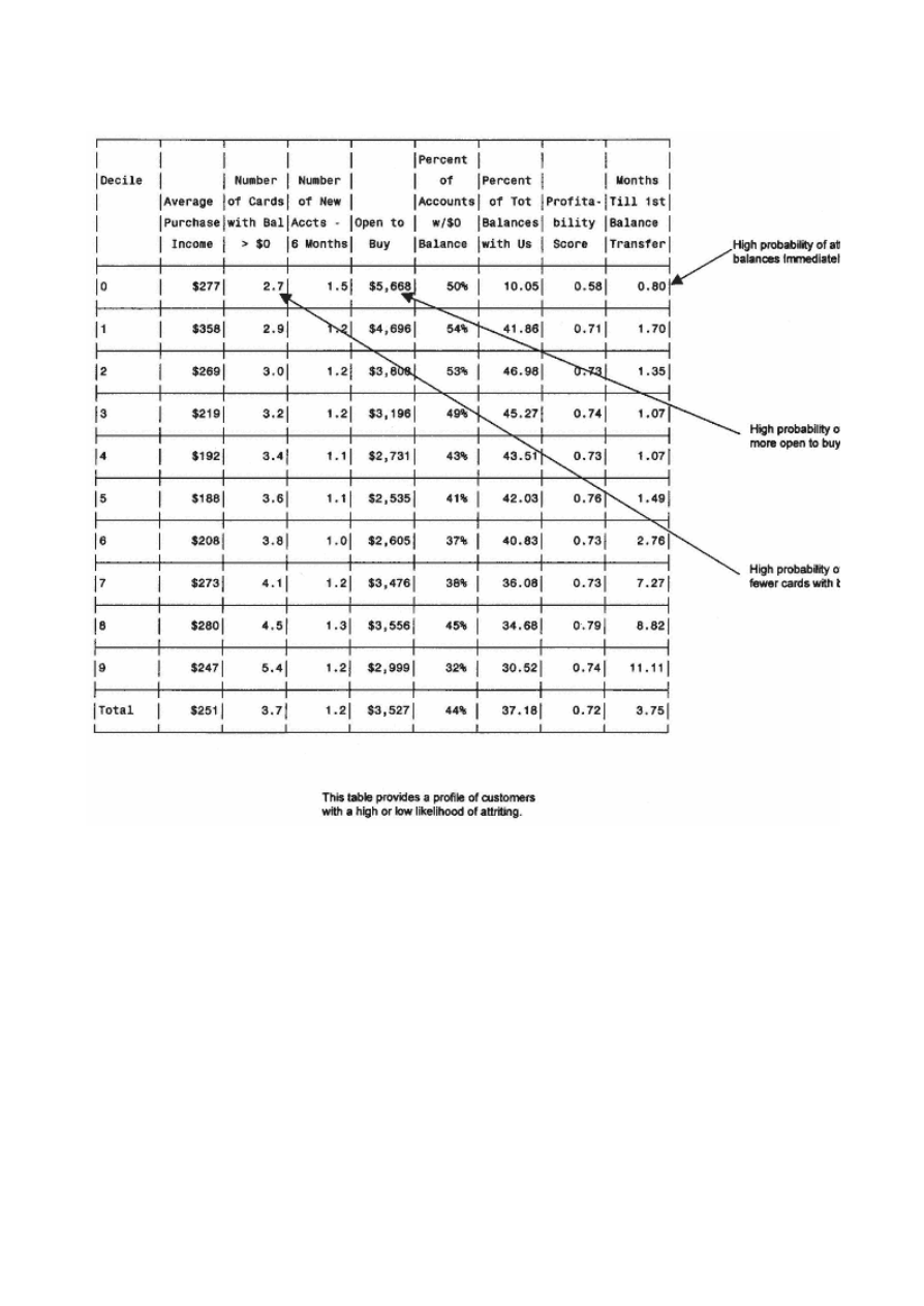
Figure

11.11

Customer

profile

decile.

/rts = 10 row=float box = ' Decile';
run;

Figure 11.11 displays the average values by decile. Notice how some variables have definite trends while others are less variable. You
could say that a person who is likely to churn has the following characteristics:

•

Fewer cards with balances

•

More new accounts with competitors

•

More ''open to buy" or room on their existing cards

•

Higher percentage of accounts with $0 balance

•

Low percentage of balances with Rowan

•

Low profitability score (based on prior model)

•

Moved balances to Rowan quickly following prior balance transfer offer

This information is quite useful in helping Rowan understand how its customers think and what might be motivating their behavior. This
can lead to smarter marketing decisions, greater customer loyalty, and higher profits.

Page 276

Optimizing Customer Profitability

Many factors influence credit card profitability. Most revolvers are profitable, but so are some transactors. The
following formula details one method for calculating 12-month credit card profitability:

Assumptions

•

Behavior for next 12 months will mimic behavior for past 12 months.

•

Risk adjustment is a function of current status and historical trends.

•

Attrition adjustment is independent of market pressures.

Values Needed for Calculation

1. Average daily balance.

2. Net purchases (purchases – returns).

3. Finance charges.

4. Late, over-limit, cash advance, annual, and miscellaneous fees.

5. Attrition probability based on churn model score.

6. Charge -off probability based on risk score.

Components of Profit and Loss

•

Fee Income (#4)— Sum of fees for prior 12 months. Value assumes similar behavior for next 12

months.

•

Finance charges (#3)— Not a straight function of balance as all balances may not be at same rate.

•

Interchange income (1.44% × #2)— Fee charged to retailer or point of sale vendor for use of card.

•

Cost of Funds (5.42% × #1)— Reflects market prices and bank's borrowing power.

•

Attrition adjustment (#5 × #3)— Probability of attrition from model is based on rate increase. Customer typically

moves entire balance resulting in lost finance charges.

•

Charge-off provision (#6 × #1)— Probability of charge-off based on risk model. Customer typically defaults on entire

balance.

•

Rebates and royalties (rate × #2 and/or #3)— Percent of balance or finance charges promised to customer or affinity

partner.

•

Operating expense ($45 annually)— Cost of annual account processing.

•

Taxes (38% × (A + B + C – D – E – F – G – H))— For Uncle

Sam.

Page 277

The final equation is this: One -Year Risk Adjusted Profit = A + B + C – D – E – F – G – H – I. This formula establishes
a profit value for each customer based on variable costs and revenue. When using this value to make marketing
decisions, it is important to remember that it does not consider fixed costs such as salaries and overhead.

This is an excellent formula for calculating one-year risk adjusted profit for credit card customers. One effective use of
this formula is to determine if raising interest rates will increase or decrease customer profitability. One advantage of
this formula is that it will determine the answer to this question on each individual customer. The results, however, are
more meaningful on an aggregate basis. To clarify, let's work through an example.

Let's say Jane Smith has the following profile: Average balance – $5,252; Net purchases $1,876; Finance charges –
$731; Fees – $29; Attrition probability following reprice – 38%; Charge-off probability prior to reprice – 2.2%; Rebate –
1%. Table 11.4 details the net profit calculation for Jane Smith. The second column shows that prior to a 4% increase in
APR, one -year risk adjusted profit for Jane Smith is $179.36. Now let's recalculate it after the rate increase. First we
must make the following assumptions:

•

Fees and purchases remain the same.

•

Balances decrease by probability of attrition. This is not precise on an individual basis but accurately reflects group

behavior.

Table 11.4

Effects of Reprice on Profitibility

PRE
REPRICE

POST
REPRICE
– 38%
CHURN
RATE

POST
REPRICE
– 43%
CHURN
RATE

POST
REPRICE
– 39.5%
CHURN
RATE

Average balance

$5,252.00

$3,256.24

$2,993.64

$3,177.46

Net purchases

$1,876.00

Finance charge

$ 731.00

$ 583.47

$ 536.42

$ 569.35

Fee income

$ 29.00

Attrition probability

38%

43%

39.5%

Charge-off provision

2.2%

2.8%

Rebate

Pretax profit

$ 289.29

$ 295.89

$ 272.91

$ 288.99

Taxes

$ 109.93

$ 112.44

$ 103.71

$ 109.82

Net profit

$ 179.36

$ 183.45

$ 169.21

$ 179.18

Page 278

•

Probability of charge-off increases by 25% following reprice.

•

Customers that are in financial trouble will usually let their higher rates cards go into default first.

The third column shows the profits following the reprice. At a 38% probability of churn, it would be marginally
profitable to increase Jane's interest rate by 4%. The fourth column, however, tells a different story. If the probability of
churn is 43%, the reprice would make Jane less profitable. In fact, we find the exact probability of churn at which the
reprice will not affect profits for Jane Smith is approximately 39.5%. This measure can be calculated for each customer
giving Rowan Royal the ability to enact one-to-one customer relationship management that optimizes profits for the
entire customer portfolio.

Retaining Customers Proactively

The same techniques that are used to increase profits with rate increases can be used to improve customer loyalty.
Consider the previous example where we determined how to increase profits by predicting which customers would be
profitable following a rate increase. We can use the same formula to evaluate incentives for customers to build balances.
For example, we could develop a model that predicts which customers will increase balances following a rate decrease
or some other incentives like higher rebates or air miles. The techniques for calculating profit and managing name
selection are the same.

Many of the automated campaign management tools are designed to score a customer with various embedded models
each time new information is received on a customer. This creates many opportunities to take immediate action when a
change is detected. For example, if a customer suddenly decreases their balance, their risk decreases along with their
profits. This might be a good time to offer them a lower rate along with some balance transfer incentives. Or if their risk
score suddenly drops into a risky range, you can increase their rate or limit their access to more credit. The possibilities
are endless. And the advances in technology that allow us to integrate and automate these analytic tools are rapidly
changing the way we manage our customers. It is becoming impossible to survive without them.

Summary

Did you notice how the mechanics of the attrition or churn model are similar to those of many of the other recipes?
Again, the main distinction between the models is the objective. I was able to use many of the same processing steps. I

Page 279

feel these models truly emphasize the importance of a clearly defined objective, not just from a modeling point of view,
but also from a business point of view.

Attrition or churn models are increasing in popularity as companies in all industries struggle to understand and retain
their most profitable customers. Along with response and risk models, churn models are becoming an integral part of
campaign management both manual and automated. With only slight modification, these techniques will work well for
companies in all areas of financial services as well as utilities, telcos, high-tech, retail, publishing, catalog, gaming, and
travel.

Before we begin the next recipe, take a break and work up an appetite. In the next chapter, I build a lifetime value
model. It's a high calorie treat!

Page 281

Chapter 12—
Targeting Profitable Customers:
Modeling Lifetime Value

In the early years of direct marketing, much of the growth in revenue took place through the acquisition of new
customers. Today, however, markets are more saturated. New customers are gained mainly at the expense of
competitors. This makes it more difficult and expensive to acquire new customers. To compensate, many companies are
relying on their current customer base to generate the bulk of their profits. They are staying competitive by placing more
emphasis on developing new products and services to offer to their existing customers. This not only affects the value of
existing customers, but it changes the value of a potential customer or prospect.

As a result, companies are willing to spend more to attract new customers by focusing on long range or lifetime value
(LTV). In this chapter, I introduce the basic concepts of lifetime value. I introduce several formulas for calculating
lifetime value with applications in a variety of industries. In the last half of the chapter, I expand the net present value
(NPV) model developed in part 2. Recall that NPV assigns profits based on a single product. In this chapter, I expand
the NPV model to predict lifetime value by incorporating cross-sell and up-sell potential for each prospect through a
series of predictive models. These models are incorporated into a lifetime value calculation for our insurance prospect
base. The benefits of using lifetime value modeling are quantified by comparing the predicted profits to those in the net
present value model in chapter 7.

Page 282

What is lifetime value?

Lifetime value is the expected value of a prospect or customer over a specified period of time, measured in today's
dollars. Lifetime value is measured in various ways, depending on the industry, but basically represents future revenues
less overhead and expenses. This valuation allows companies to allocate resources based on customer value or potential
customer value.

Historically, marketing strategies were driven by the financial benefits of a single campaign. Customer profitability was
optimized by the net profits of the initial sale. But with the increased cost of acquiring customers and the expansion of
products and services to existing customers, companies are expanding their marketing strategies to consider the lifetime
value of a potential customer.

Lifetime value measurements on a customer portfolio can quantify the long-term financial health of a company or
business. In the following sidebar, William Burns, Adjunct Professor of Business Administration at San Diego State
University, explains the holistic importance of the lifetime value measure.

Uses of Lifetime Value

Lifetime value measurements are useful for both acquiring customers and managing customer relationships. For new
customer acquisition, the increased expected value allows companies to increase marketing expenditures. This can
broaden the universe of profitable prospects. Later on in this chapter, I will show how this is carried out in our life
insurance case study.

For customer relationship management, the uses of a lifetime value measurement are numerous. Once an LTV is
assigned to each customer, the customer database can be segmented for a variety of purposes. In many cases, the 80/20
rule applies— that is, 20% of the customer base is generating 80% of the profits.

Armed with this information, your company is able to take actions or avoid an action based on the long-term benefit to
the company. Marketing programs can be tailored to different levels of profitability. For example, banks and finance
companies use LTV to determine risk actions such as rate increases or line adjustments. Multiline companies use LTV to
sequence product offers. Many companies offer premium customer service, such as an 800 number, to their high-value
customers. Whatever the action or treatment, many companies are using LTV to optimize their customer relationship
management.

Page 283

Why Is Lifetime Value Important for Marketing Decisions?

Economists have long argued that business decisions should seek to maximize value for shareholders and
that all projects can and should be systematically examined in this light. Consistent with this perspective,
marketers must recognize that their efforts should be guided by value maximization as well. Ideally, the
practice of value optimization should begin during the market segmentation stage. Experience has shown that
customers vary widely in their value to a business due to differing spending patterns, loyalty, and tendency to
generate referrals. Hence, segmentation should include considerations of customer lifetime worth. Similar
arguments can be made for other marketing activities. As it turns out, the lifetime value (LTV) of a customer
represents an attractive metric for marketing managers for the following reasons:

•

All factors being equal, increasing the LTV of customers increases the value of the firm.

•

Customer LTV can be directly linked to important marketing goals such as sales targets and customer

retention.

•

LTV calculations require the marketer to take a long and comprehensive view of the customer.

•

LTV accounts for differences in risk level and timing of customer profit streams.

The economic logic behind maximizing customer value is based on the notion that every marketing action
has an opportunity cost. That is, investors who help capitalize a business can earn returns from a number of
sources both within and outside the company. To cultivate loyal investors, it is not enough to simply have
revenues exceed costs and call this a profitable marketing venture. A simple example illustrates this point.

Suppose I am considering a promotion designed to acquire new customers. This program may at first appear
justified because total revenues are projected to soon exceed total costs based on some break-even analysis.
After forecasting the likely return on investment (adjusted for risk), though, I may discover that the long-
term economic impact of, say, increasing retention of our most valuable customers is much higher. Had I
gone ahead with the promotion, I might have destroyed rather than improved economic value. How many
marketing managers think in these terms? It's not a trivial question, given that the most economically viable
firms will attract the best customers, employees, and investors over time and thereby will outdistance their
competitors.

Team-Fly

Page 284

Components of Lifetime Value

Lifetime value can be calculated for almost any business. In its simplest form, it has the following base components:

Duration. The expected length of the customer relationship. This value is one of the most critical to the results and
difficult to determine. And like many aspects of modeling, there are no hard-and-fast rules for assigning duration. You
might think that a long duration would be better for the business, but there are two drawbacks. First, the longer the
duration, the lower the accuracy. And second, a long duration delays final validation. See the accompanying sidebar, for
a discussion by Shree Pragada on assigning duration.

Time period. The length of the incremental LTV measure. This is generally one year, but it can reflect different renewal
periods or product cycles.

Revenue. The income from the sale of a product or service.

Costs. Marketing expense or direct cost of product.

Discount rate. Adjustment to convert future dollars to today's value.

Some additional components, depending on the industry, may include the following:

Renewal rate. The probability of renewal or retention rate.

Referral rate. The incremental revenue generated.

Risk factor. The potential losses related to risk.

Assigning Duration

Shree Pragada, Vice President of Customer Acquisition for Fleet Credit Card Bank, discusses some
considerations for assigning duration in the credit card industry.

With customer relationship management (CRM) becoming such a buzzword and with the availability of a
variety of customer information, CRM systems have become quite widespread. In estimating customer or
prospect profitability in CRM systems, the duration for the window of financial evaluation appears to be
fuzzy. Should it be six months, one year, three years, six years, or longer? Even within an organization, it can
be noticed that different durations are being used across different departments for practically the same
marketing campaign. The

Page 285

finance department may want to have CRM systems configured to estimate profitability for as much as six
or seven years, assuming that a portfolio with 15 –20% account attrition will continue to yield value for
about six to seven years. The risk management department may be interested in three- to four-years'
duration as credit losses take about three years to stabilize. Some marketing departments would be
comfortable executing million-dollar campaigns with just response predictions that span just over three to
four months. Everyone has a different duration for evaluating expected profitability and for the logical
explanations why that duration could be better. So, how long should I aim to evaluate customer profitability
and why?

For starters, there is no cookie-cutter solution for the best duration across all customer profitability systems.
For instance, the mortgage industry should develop profitability systems that span over several years while
the credit card industry might benefit from shorter and much more focused duration. And, within an industry
different marketing campaigns will need different durations depending on the campaign goals and the profit
drivers. I will look at the credit card industry to elaborate on this point.

Consider two marketing campaigns:

•

Rate Sale Offer for six months to improve purchase activity by giving a promotional annual percentage rate

for a short period of time.

•

Balance Transfer Offer for two years to increase card receivables by enticing customers to transfer balances

from competitors through low-rate balance transfer offers.

The difference that I wish to show between these marketing offers is that Offer 1 is good for only six months
while Offer 2 is good for two years. Studying the performance of these marketing offers will show that
customer behavior stabilizes or regresses to its norm sooner for Offer 1 than for Offer 2. The reasons are
quite obvious.

Let me digress a little into what constitutes a success or failure in a marketing campaign. Every marketing
campaign will alter the normal customer behavior by a certain degree. When customers respond to marketing
offers, say a balance transfer offer, they will bring additional balances, pay more finance charges, probably
even use their cards more. They will digress from their norm for a "duration" after which they will regress to
their normal account behavior. The more they digress, the more profitable they tend to be. (The case of
negative behavior has been discounted for simplicity.) The success of a marketing program depends on how
much customers have digressed from their norm and how many — in short, the "positive incremental value."
Because CRM systems are primarily put to task to configure/identify marketing programs to maximize

continues

Page 286

(Continued)

profitability, attention should be paid to this ''duration" for which the marketing programs tend to alter
overall customer behavior.

To summarize, as profitability is estimated by modeling the many customer behaviors, the "duration" should
not be more than the duration for which any of the underlying behaviors can be modeled comfortably. For
instance, credit losses can be estimated fairly for over 3 years, but account balance fluctuations can hardly be
modeled past 18 months to 2 years. So this would limit the duration for a CRM system in the Card Industry
to about 2 years. An alternative to trying to model difficult behavior past the comfortable duration is to
estimate a terminal value to extend the duration to suit traditional financial reporting.

Applications of Lifetime Value

As mentioned previously, the formulas for calculating lifetime value vary greatly depending on the product and industry.
In the following cases, Arthur Middleton Hughes, Director of Strategic Planning at M\S Database Marketing, illustrates
some unique calculations. In addition, he shows how to calculate the discount rate for a particular business.

Lifetime Value Case Studies

Lifetime value has become a highly useful method for directing marketing strategies that increase customer lifetime
value, retain customers that have high lifetime value, and reprice or discard customers with negative lifetime value. The
following cases highlight some uses of LTV calculations.

Business-to-Business Marketing

Lifetime value tables for business-to -business customers are easy to develop. To show how this is done, let's develop the
lifetime value of customers of an artificial business, the Weldon Scientific Company, that sells high-tech equipment to
factories and laboratories.

Let's explain some of the numbers in Table 12.1. Year 1 represents the year of acquisition, rather than a calendar year.
Year 1 thus includes people acquired in several different years. Year 2 is everybody's second year with Weldon. I am

Page 287

Table 12.1

Lifetime Value Table for Business to Business

YEARS 1

YEAR 2

YEAR 3

Customers

20,000

12,000

7,800

Retention Rate

60.00%

65.00%

70.00%

Orders/year

1.8

2.6

3.6

Avg. Order Size

$2,980

$5,589

$9,106

Total Revenue

$107,280,000

$174,376,800

$255,696,480

Direct Cost %

70.00%

65.00%

63.00%

Costs

$75,096,000

$113,344,920

$161,088,782

Acquisition Costs $630

$87,696,000

$113,344,920

$161,088,782

Total Costs

$87,696,000

$113,344,920

$161,088,782

Gross Profit

$19,584,000

$61,031,880

$94,607,698

Discount Rate

1.13

1.81

2.53

Net Present Value Profit

$17,330,973

$33,719,271

$37,394,347

Cumulative NPV Profit

$17,330,973

$51,050,244

$88,4444,591

Customer Lifetime Value

$867

$2,553

$4,422

assuming that Weldon has acquired 20,000 business customers, including a number of independent distributors. A year
later, only 12,000 of these customers are still buying. That means that Weldon's retention rate is 60%. Over time, the
retention rate of the loyal Weldon customers who are still buying goes up.

The average customer placed an average of 1.8 orders in their year of acquisition, with an average order value of $2,980.
As customers became more loyal, they placed more orders per year, of increasing size.

The acquisition cost was $630 per customer. The cost of servicing customers came down substantially after the first
year. Most interesting in this chart is the discount rate, which is developed in a separate table. The discount rate is
needed because to compute lifetime value I will have to add together profit received in several different years. Money to
be received in a future year is not as valuable as money in hand today. I have to discount it if I want to compare and add
it to current dollars. That is the purpose of the discount rate summarized in Table 12.2.

Page 288

Table 12.2 Discount Rate by Year

YEAR 1

YEAR 2

YEAR 3

Year

Risk Factor

1.8

1.5

1.4

Interest Rate

8.00%

A/R Days

Discount Rate

1.13

1.81

2.53

The formula for the discount rate is this:

It includes the interest rate, a risk factor, and a payment factor. In the first year, Weldon tries to get new customers to
pay up front, relaxing to a 60-day policy with subsequent orders. For established customers, 90-day payment is
customary. The risk factor drops substantially with long -term customers. The combination of all of these factors gives
Weldon a sophisticated discount rate that is responsive to the business situation that it faces.

When the Repurchase Cycle Is Not Annual

The retention rate is typically calculated on an annual basis. A 60% retention rate means that of 10,000 customers
acquired in Year 1, there will be only 6,000 customers remaining as active customers in Year 2. This is easy to compute
if customers buy every month or once a year. But what is the annual retention rate if 50% of the customers buy a product
only every four years? This is true in many business-to-business situations. Here a formula is necessary. The formula is
this:

RR is the annual retention rate, RPR is the repurchase rate, and Y is the number of years between purchases. The
following two examples illustrate the use of this formula for automobile purchases.

Automobile Purchase by One Segment

A segment of Buick owners buys a new car every four years. About 35% of them buy a Buick, and the balance buys
some other make of car. What is their annual retention rate?

Page 289

Automobile Purchase by Several Segments

Buick owners can be divided into four segments: those who buy a new car every one year, two years, three years, and
four years. Their respective repurchase rates are shown in Table 12.3.

Table 12.3

Table Repurchase Rates by Segment

SEGMENT

YEARS

BETWEEN

PURCHASE

REPURCHASE

RATE

ANNUAL

RETENTION

ACQUIRED

CUSTOMERS

RETAINED

CUSTOMERS

55.00%

90,346

49,690

45.00%

67.08%

170,882

114,631

40.00%

73.68%

387,223

285,308

35.00%

76.92%

553,001

425,347

Total

72.83%

1,201,452

874,976

Table 12.3 provides some interesting information. The repurchase rate of those who buy a Buick every year seems much
higher than that of those who wait four years between automobile purchase. Their annual retention rate, however, is far
lower.

Restaurant Patrons by Week

A business-area restaurant had a regular clientele of patrons who ate there almost every day. The restaurant decided to
try database marketing. Its staff set up a system to gather the names of their customers and gave points for each meal.
They discovered that they were losing about 1% of their clients every week. What was their annual retention rate? The
formula is the same:

In this case, the repurchase rate is 99%, and the period involved is 1/52 of a year, so the formula becomes:

This tells us that the restaurant's annual retention rate is 59.3%.

Page 290

Calculating Lifetime Value for a Renewable Product or Service

William Burns contributed the following simple formula for calculating lifetime value for a renewable product or
service.

1. Forecast after-tax profits over the lifetime of the customer group. Begin with determining the possible lifespan of a
customer and the typical billing cycle. Useful forecasts must be based on a sound theory of customers in your
organization.

2. Determine the expected rate of return (r) for the marketing project in mind. The firm's finance group is the best source
of help, but outside financial expertise can also be used.

3. Calculate the net present value (NPV) of the CFt over the lifetime of the customer group. The general formula to do
this calculation is as follows:

Where subscript t is the number of time periods composing the lifetime of the customer group (time period should
correspond to billing cycle). PV represents the upper limit of what should be paid to acquire a customer group.

Where CF

represents the after-tax cost of acquiring the customer group. NPV represents the actual worth of the

customer group after acquisition.

Where C is the total number of customers initially acquired. LTV represents the worth of a typical customer to the
company at the time of acquisition.

Calculating Lifetime Value:
A Case Study

As I expand the case study in Part 2 to calculate lifetime value, I will leverage knowledge gained through years of
practice by experts in the direct marketing industry. Donald R. Jackson, author of 151 Secrets of Insurance Direct
Marketing Practices Revealed (Nopoly Press, 1989), defines "Policy Holder Lifetime Value":

Policy Holder Lifetime Value is the present value of a future stream of net contributions to overhead and profit expected
from the policyholder.

Page 291

He goes on to list some key opportunities available to companies that use lifetime value for insurance marketing:

Policy Holder LTV provides a financial foundation for key management decisions:

1. Developing rates for insurance products

2. Assigning allowance for policyholder acquisition

3. Setting selection criteria for policyholder marketing

4. Choosing media for initial policyholder acquisition

5. Investing in reactivation of old policyholders

6. Assigning an asset value to your policyholder base

As I discussed earlier, prospects may be marginally profitable or even unprofitable when they first become customers.
They have expressed an interest in doing business with you, so the hard work is done. You now have an opportunity to
develop a profitable long-term relationship within which you can sell them different products (cross-sell) or more of the
same product (up -sell). To cross-sell a life insurance customer, you might try to sell the customer health or accident
insurance. An up-sell is typically an offer to increase the coverage on the customer's current policy.

In chapter 7, I calculated the net present value of a single product for a group of prospects. This produced the expected
profits for a single policy over three years. It accounted for risk and cost of mailing for the single product. In this
chapter, I incorporate the value of additional net revenue to prospects, which allows me to calculate their lifetime value.
The first step is to develop models to estimate the probability of incremental net revenue for each prospect. For clarity,
I'll call this model our Cross-Sell Up -Sell Revenues (CRUPS) model.

Case Study:
Year One Net Revenues

To develop the incremental net revenue models, I take a sample of customers, both current and lapsed, that were booked
between three and four years ago. I use their prospect information to develop three models, one model to predict
incremental net revenues for each of the first three years.

Because this is a model using customer information, I pull data from the data warehouse. Customers that were booked
between three and four years ago are identified. I extract 2,230 customers along with their information at the time of
acquisition for modeling. Additional sales, claims, and policy lapse information for the following three years are
appended from the customer files. This data has been corrected for missing values and outliers.

Page 292

The following code calculates the net revenues for each incremental year by summing the total sales reduced by the
percent of claims. The variables names are crupsyr1, crupsyr2 , and crupsyr3 for each of the three years:

acqmod.crossell;
acqmod.crossell;
crupsyr1 = sum(of sale01Y1-sale12Y1)*(1 -claimpct);
crupsyr2 sum(of sale01Y2 -sale12Y2)*(1-claimpct);
crupsyr3 sum(of sale01Y3 -sale12Y3)*(1-claimpct);
run;

The following code begins by randomly assigning a missing weight to half of the data set. Because I am planning to use
linear regression to predict additional net revenues, I must get all variables into a numeric, continuous form. The
remaining code creates indicator variables by assigning numeric values to n – 1 levels of each categorical variable. For
example, the variable pop_den has four levels: A, B, C, and missing. The three indicator variables, pop_denA ,
pop_denB , and pop_denC , have values of 0 and 1. The missing level is represented when the values for the other three
indicator variables equals 0:

data acqmod.crossell;
set acqmod.crossell;
if ranuni(5555) < .5 then splitwgt = 1; else splitwgt = .;

pop_denA = (pop_den = 'A');
pop_denB = (pop_den = 'B');
pop_denC = (pop_den = 'C');
trav_cdd = (trav_cd = '1');
bankcrdd = (bankcrd = 'Y');
deptcrdd = (deptcrd = 'Y');
fin_cod = (fin_co = 'Y');
pre_crdd = (pre_crd = 'Y');
upsccrdd = (upsccrd = 'Y');
apt_indd = (apt_ind = 'Y');
sgle_ind = (sgle_in = 'Y');
finl_idm = (finl_id = 'M');
finl_idn = (finl_id = 'N');
hh_indd = (hh_ind = 'H');
gend_m = (gender = 'M');
driv_inA = (driv_in = 'A');
driv_inN = (driv_in = 'N');
mob_indN = (mob_ind = 'N');
mob_indY = (mob_ind = 'Y');
mortin1M = (mortin1 = 'M');
mortin1N = (mortin1 = 'N');
mortin1Y = (mortin1 = 'Y');
autoin1M = (autoin1 = 'M');
autoin1N = (autoin1 = 'N');
autoin1Y = (autoin1 = 'Y');
childind = (childin = 'Y');
run;

Page 293

Similar to the processing in chapter 5, the following code finds the best transformation for each continuous variable. I
create predictors for the first-year model using the following code. The second- and third-year models are created using
the same techniques:

data acqmod.agedset;
set acqmod.crossell(keep=pros_id infd_age crupsyr1);

age_sq = infd_age**2;
age_cu = infd_age**3;
age_sqrt = sqrt(infd_age);
age_curt = infd_age**.3333;
age_log = log(max(.0001,infd_age));
| | | | |
| | | | |
age_tani = 1/max(.0001,tan(infd_age));
age_sini = 1/max(.0001,sin(infd_age));
age_cosi = 1/max(.0001,cos(infd_age));

run;

Because I am using continuous values to predict a continuous value, I use linear regression. In SAS the procedure is
called PROC REG:

title "Regression on Inferred Age";
proc reg data=acqmod.agedset;
model crupsyr1 = infd_age
age_sq age_cu age_sqrt age_curt age_log
age_tan age_sin age_cos age_inv age_sqi
age_cui age_sqri age_curi age_logi
age_tani age_sini age_cosi
/ selection = stepwise stop = 2 details;
run;

In Figure 12.1, I see that the best form of the variable Inferred Age is the inverse cube root (age_cui). This will be a
candidate in the final model. This step is repeated for all the continuous variables. The following code sorts and
combines the data sets with the best transformation of each continuous variable:

%macro srt(svar);
proc sort data = acqmod.&svar.dset;
by pros_id;
run;

%mend;
%srt(age)
%srt(inc)
%srt(hom)
%srt(toa)
%srt(tob)

Team-Fly

Page 294

%srt(inq)
%srt(top)
%srt(crl)

proc sort data = acqmod.crossell;
by pros_id;
run;

data acqmod.crs_vars;
merge
acqmod.crossell
acqmod.agedset(keep = pros_id age_cui infd_agf)
acqmod.incdset(keep = pros_id inc_curt inc_estf)
acqmod.homdset(keep = pros_id hom_log hom_equf )

Figure

12.1

Regression

output

for

Inferred

Age.

Page 295

acqmod.toadset(keep = pros_id toa_sqrt tot_accf)
acqmod.tobdset(keep = pros_id tob_curt tot_balf)
acqmod.inqdset(keep = pros_id inq_log inql6mof)
acqmod.topdset(keep = pros_id top_sqrt tot_opaf)
acqmod.crldset(keep = pros_id crl_log credlinf);
by pros_id;
run;

The following code uses linear regression to find the best predictors for First Year Cross-Sell Up -Sell Revenues
(crupsyr1 ).

proc reg data=acqmod.crs_vars;
weight splitwgt;
model crupsyr1 = actopl6 age_fil amtpdue hom_equ inc_est infd_ag inql6m
no30day no90eve nobkrpt totopac tot_acc tot_bal pop_denA pop_denB
pop_denC trav_cdd bankcrdd deptcrdd pre_crdd upsccrdd apt_indd sgle_ind
finl_idm finl_idn hh_indd gend_m driv_inA driv_inN mob_indN mob_indY
mortin1M mortin1N mortin1Y autoin1M autoin1N autoin1Y childind age_cui
inc_curt hom_log toa_sqrt tob_curt inq_log top_sqrt crl_log
/selection=rsquare best=2 stop=20;
run;

In Figure 12.2, see how the score selection process in logistic regression, the selection=rsquare option calculates the best
models for every possible number of variables. Best=2 was used to produce two models for each number of variables.
Stop=20 was used to limit the number of possible models. The 15 -variable model with the highest r-square was selected
as the final model. The following code reruns the regression to create an output data set that is used for validation:

proc reg data=acqmod.crs_vars outest=acqmod.regcoef1;
weight splitwgt;
model crupsyr1 = AGE_FIL BANKCRDD DEPTCRDD UPSCCRDD APT_INDD GEND_M
DRIV_INA DRIV_INN MORTIN1M MORTIN1Y AGE_CUI TOA_SQRT INQ_LOG TOP_SQRT
CRL_LOG;
output out=acqmod.out_reg1 p=pred r=resid;
run;

Next, I sort and create deciles to see how well the model predicts Year One Net Revenue:

proc sort data=acqmod.out_reg1;
by descending pred;
run;

proc univariate data=acqmod.out_reg1(where=(splitwgt = .)) noprint;;
var pred;
output out=preddata nobs=nobs;
run;

Page 296

data acqmod.val_dec;
set acqmod.out_reg1;
if (_n_ eq 1) then set preddata;
if _N_ < .1*nobs then val_dec = 0; else
if _N_ < .2*nobs then val_dec = 1; else
if _N_ < .3*nobs then val_dec = 2; else
if _N_ < .4*nobs then val_dec = 3; else
if _N_ < .5*nobs then val_dec = 4; else
if _N_ < .6*nobs then val_dec = 5; else
if _N_ < .7*nobs then val_dec = 6; else
if _N_ < .8*nobs then val_dec = 7; else
if _N_ < .9*nobs then val_dec = 8; else
val_dec = 9;
records=1;
run;

title1 "Gains Table -
Year One Cross Sell / Up Sell Revenues";

PROC tabulate data=acqmod.val_dec;
class val_dec;
var pred records crupsyr1;
table val_dec='Decile' all='Total',
records='Prospects'*sum=' '*f=comma10.

Figure

12.2

Linear

regression

output

for

selection=rsquare.

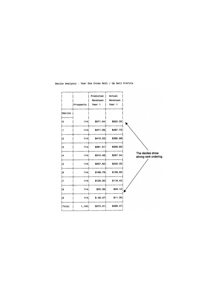
Page 297

pred='Predicted Revenues Year 1'*(mean=' '*f=dollar11.2)
crupsyr1 ='Actual Revenues Year 1'*(mean=' '*f=dollar11.2)
/rts = 9 row=float;
run;

See in Figure 12.3 that the model produces strong rank -ordering of names by 1st Year Net Revenues. The following
code plots the predicted values against the actual values.

proc summary data=acqmod.val_dec;
var pred crupsyr1;
class val_dec;
output out=acqmod.valplot mean=predmean crupmean;
run;

Figure

12.3

Decile

analysis

Year

One

Cross -Sell

Up-Sell

Model.

proc plot data=acqmod.valplot;
plot predmean*crupmean;
run;

The results can be seen in Figure 12.4, which shows a plot of the average decile's values for the predicted and actual Net Revenue. The
near diagonal plot shows strong predictive power.

The previous process is repeated for years 2 and 3. The final calculations are combined with the data set that was scored in chapter 7.

Lifetime Value Calculation

I'm now ready to apply our three new models to the campaign data from chapter 7. Recall that I had a data set, acqmod.test
of a 5,000-record ran-

Figure

12.4

Plot

average

predicted

and

actual

decile.

Page 299

dom sample from the score file at the outside list company. The following code uses PROC SCORE to apply the three
mode scores to the data sample:

proc score data=acqmod.test
out=acqmod.crup1ys1 predict score=acqmod.regcoef1 type=parms;
id pros_id records;
VAR AGE_FIL BANKCRDD DEPTCRDD UPSCCRDD APT_INDD GEND_M DRIV_INA DRIV_INN
MORTIN1M MORTIN1Y AGE_CUI TOA_SQRT INQ_LOG TOP_SQRT CRL_LOG;
run;

proc score data=acqmod.test
out=acqmod.crup1ys2 predict score=acqmod.regcoef2 type=parms;
id pros_id records;
VAR ACTOPL6 INC_EST TOTOPAC TOT_ACC DEPTCRDD PRE_CRDD UPSCCRDD GEND_M
DRIV_INA DRIV_INN MOB_INDY AGE_CUI;
run;

proc score data=acqmod.test
out=acqmod.crup1ys3 predict score=acqmod.regcoef3 type=parms;
id pros_id records;
VAR ACTOPL6 INC_EST NO30DAY NO90EVE DEPTCRDD PRE_CRDD UPSCCRDD GEND_M
MOB_INDY AUTOIN1N HOM_TANI TOP_SQRT;
run;

The scoring programs create three separate files. The following code sorts the three data sets using pros_id as a match
key.

%macro srt(dsn);
proc sort data = acqmod.&dsn;
by pros_id;

run;
%mend;
%srt(crup1ys1)
%srt(crup1ys2)
%srt(crup1ys3)
%srt(test)

Next I need to merge our three scored data sets with our main data set (acqmod.test). The variable, model1, is the default
name for the Net Revenue predicted by each model. I need to rename the variable when I merge the results from the
three models. I name them crupsyr1 , crupsyr2 , crupsyr3 to match the original names:

data acqmod.ltv;
merge acqmod.crup1ys1(rename=(model1=crupsyr1 ))
acqmod.crup1ys2(rename=(model1=crupsyr2 ))

Page 300

acqmod.crup1ys3( rename=
(model1=crupsyr3)) acqmod.test;
by pros_id;

The next step is to calculate the discounted profits for the next three years. This is a function of several factors. First, I
have the cost of additional offers over the next three years. I have the variables off_yr1, off_yr2, off_yr3 that represent
the number of times each customer was mailed in each year. They are multiplied by the cost of a mailing, $.78. A yearly
account maintenance fee of $20 is subtracted from each year's net revenues. And, finally, it is divided by the discount
rate.

year1pr = (crupsyr1 -.78*off_yr1 - 20)/1.15;
year2pr = (crupsyr2 -.78*off_yr2 - 20)/(1.15*1.15);
year3pr = (crupsyr3 -.78*off_yr3 - 20)/(1.15*1.15*1.15);

Recall the risk matrix that assigns a risk adjustment based on a combination of gender, marital status, and age. The
following code creates a variable called risk_adj to use in the LTV calculation:

if gender = 'M' then do;
if marital = 'M' then do;
if infd_ag2 < 40 then risk_adj = 1.09;
else if infd_ag2 < 50 then risk_adj = 1.01;
else if infd_ag2 < 60 then risk_adj = 0.89;
else risk_adj = 0.75;
end;
else if marital = 'S' then do;
if infd_ag2 < 40 then risk_adj = 1.06;
| | | | |
| | | | |
else if marital = 'W' then do;
if infd_ag2 < 40 then risk_adj = 1.05;
else if infd_ag2 < 50 then risk_adj = 1.01;
else if infd_ag2 < 60 then risk_adj = 0.92;
else risk_adj = 0.78;
end;
end;

Now I'm ready to calculate the lifetime value. From chapter 7, I know that the average net present value of the initial
policy is $811.30. The lifetime value (ltv_3yr) is derived by multiplying the probability of becoming active (pred_scr)
times the risk adjustment index (risk_adj) times the sum of the discounted profits from the initial policy (prodprof) and
the expected profits for the following years minus the initial marketing expense:

prodprof = 811.30;
ltv_3yr= pred_scr*risk_adj*(prodprof + year1pr + year2pr + year3pr) -
.78;
run;

Page 301

To create a gains table based on lifetime value, I sort and create deciles based on the newly derived variable, ltv_3yr.

proc sort data=acqmod.ltv;
by descending ltv_3yr;
run;

proc univariate data=acqmod.ltv noprint;
var ltv_3yr;
output out=preddata nobs=nobs;
run;

data acqmod.val_ltv;
set acqmod.ltv;
if (_n_ eq 1) then set preddata;
if _N_ < .1*nobs then val_dec = 0; else
if _N_ < .2*nobs then val_dec = 1; else
if _N_ < .3*nobs then val_dec = 2; else
if _N_ < .4*nobs then val_dec = 3; else
if _N_ < .5*nobs then val_dec = 4; else
if _N_ < .6*nobs then val_dec = 5; else
if _N_ < .7*nobs then val_dec = 6; else
if _N_ < .8*nobs then val_dec = 7; else
if _N_ < .9*nobs then val_dec = 8; else
val_dec = 9;
records=1;
run;

PROC tabulate data=acqmod.val_ltv;
class val_dec;
var ltv_3yr pred_scr records crupsyr1 crupsyr2 crupsyr3 year1pr year2pr
year3pr risk_adj;
table val_dec='Decile' all='Total',
records='Prospects'*sum=' '*f=comma9.
pred_scr='Predicted Active Rate'*(mean=' '*f=9.5)
(crupsyr1 ='Predicted Customer C/U Revenues Year 1'
crupsyr2 ='Predicted Customer C/U Revenues Year 2'
crupsyr3 ='Predicted Customer C/U Revenues Year 3')
*(mean=' '*f=dollar11.5)
risk_adj = 'Risk Index'*(mean=' '*f=6.2)
(year1pr ='Discounted Customer C/U Profits Year 1'
year2pr ='Discounted Customer C/U Profits Year 2'
year3pr ='Discoutned Customer C/U Profits Year 3')
*(mean=' '*f=dollar11.5)
ltv_3yr = 'Total 3-Year Lifetime Value'
*(mean=' '*f=dollar8.5)
/rts = 8 row=float;
run;

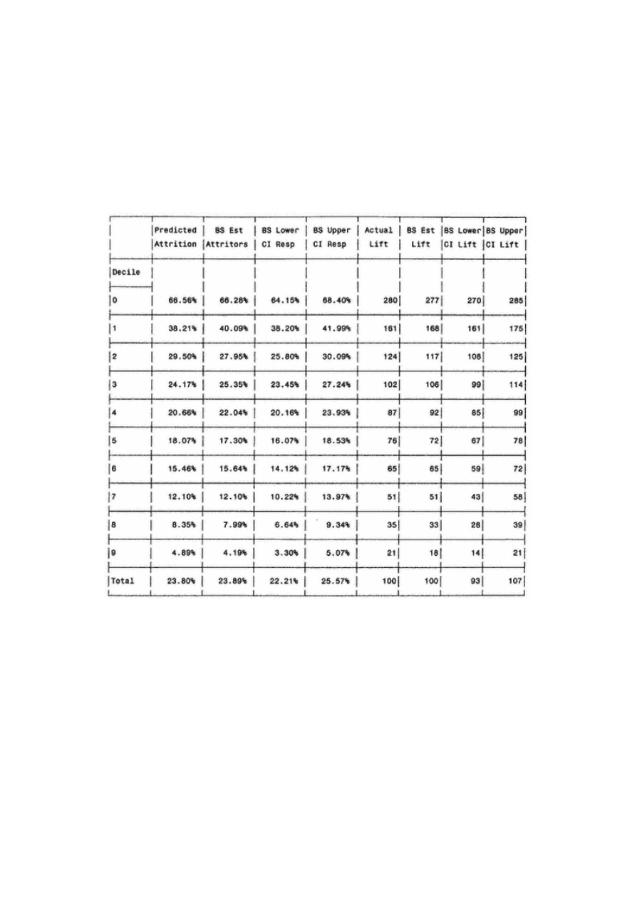
Page 302

The decile analysis in Figure 12.5 displays a wealth of information. Recall that in chapter 7 I calculated the average
three-year net present value of a life insurance prospect based on the purchase of a single policy. In Figure 12.5, I have
the same sample of names. But this time, I've included all expected customer profits for the three-year period following
activation. Notice that the ranking of ''active rate" is still monotonically decreasing, but the slope is not as strong. The
average risk indices are also slightly different from those in Figure 7.6. But the far right column, Total 3-Year Lifetime
Value, shows good profitability in the top deciles.

Notice that the lifetime value (LTV) is positive through decile 7. Compare this to Figure 7.6, where the net present value
was positive only through decile 5. If name selection was simply based on mailing to prospects with positive value,
using lifetime value could expand the names selection to capture two addi-

Figure

12.5

Decile

analysis

for

lifetime

value.

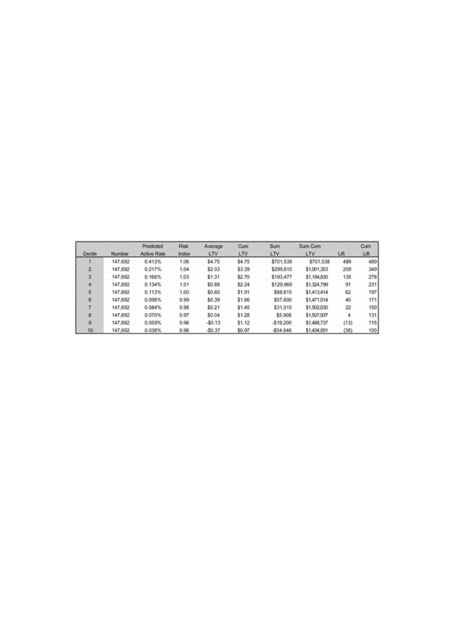
Page 303

tional deciles. Let's say the company has a hurdle rate of $.80. In other words, the company requires $.80 in income to
cover fixed expenses. The single policy NPV selection (Figure 7.6) could justify selecting only two deciles, but the LTV
selection (Figure 12.6) could select four deciles and still be profitable.

Now that I have an expected lifetime value measurement for each prospect, I carry this through to calculate cumulative
average lifetime value, sum of lifetime value per decile, and cumulative sum of lifetime value. These allow us to
measure additional gains from the use of the lifetime value measurement in the prospect file. For example, by using
lifetime value I can mail deeper into the file and capture additional expected profits. Again, comparing decile 7 to decile
5 as a cut-off point, I can expect an additional $88,616 in profits. If I want to consider the $.80 hurdle rate, I compare
expected profits through decile 4 versus decile 2. These additional 2 deciles allow for a $323,446 increase in expected
profits. Either way, predicting lifetime value is truly more powerful in selecting profitable names.

Figure 12.7 displays a visual account of the power of the lifetime value model. Notice the model's ability to concentrate
the actives and high lifetime value prospects into the lower deciles. The active rate drops quickly in the first few deciles.
Lifetime value increases steadily until it peaks in decile 8.

Summary

Well, I hope you didn't get burned! This was the most advanced recipe in the book. But what power! As you can see,
lifetime value brings together many of the other measurements used in marketing and business decision making. By

Figure

12.6

Lifetime

value

gains

table.

Team-Fly

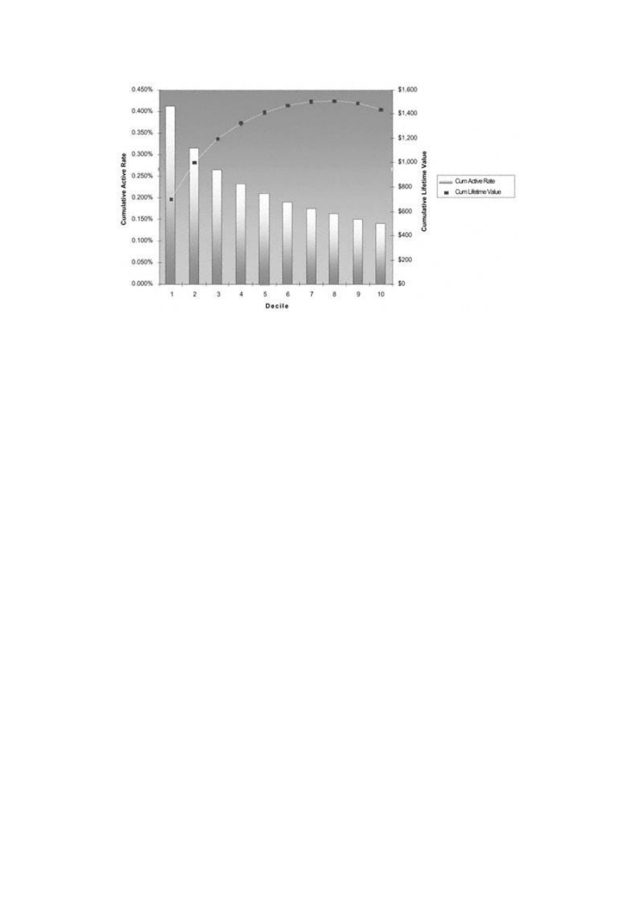
Page 304

Figure

12.7

Lifetime

value

gains

chart.

using a measure of lifetime value, no matter what the industry, you can gain accuracy at every level. You need to
identify all the components carefully. And it requires a lot of planning and analysis. But it can be used in many areas of
the business from marketing and name selection to pricing, risk action and analysis, and asset valuation of your customer
base. No matter what industry you're in, it's worth calculating lifetime value and incorporating it into your business
model.

Page 305

Chapter 13—
Fast Food:
Modeling on the Web

Why do you buy fast food? Speed? Convenience? Fast food restaurants are designed to handle large volumes of food in
a quick and efficient manner. Think of this food as data, and you have a direct parallel to the Web. The volume of data
captured from the Web is increasing exponentially. And speed is becoming a critical competitive factor. This creates
many opportunities and challenges for modeling and analysis. The opportunities arise from the sheer volume of data.
The challenges are due to the incredible speed at which the data is generated. This combination deems it necessary to
use automated modeling software to be competitive.

All of the modeling techniques I've described in prior chapters require considerable time and management. To be
effective and competitive on the Web, though, models need to be developed or available in real time. In other words,
they need to be created and utilized immediately and automatically. This chapter is not a recipe per se. Instead, my goal
is to share several ways that automated modeling and analysis software is being used to manage and redefine the
customer experience on the Web.

In this chapter, I invited several contributors who I feel are leading the industry in Web mining and modeling to share
their views. The chapter opens with a discussion of some common objectives in Web mining and modeling. The next
section outlines the steps to the most common type of Web mining, Web usage mining. An overview is provided for
several of the techniques. The remainder of

Page 306

the chapter describes some ways in which Web mining and e-commerce are changing the dynamics of marketing in the
areas of branding and increasing customer loyalty.

Web Mining and Modeling

I would like to begin by distinguishing between Web mining and Web modeling. Web mining consists of analyzing Web
traffic or usage behavior for customers and prospects. Web modeling involves using the results of Web analysis to
define business rules that can be used to shape the customer experience. As you will see in the discussion that follows,
some tools exist that allow certain types of modeling to be done in real time. In other words, certain models are built and
implemented within the same user session. Other, more traditional models, such as predictive models, segmentation, and
profiling, are built offline with the resulting scores or segments accessible during the online session.

The steps for mining Web data are familiar. As you might expect, defining the objective is the first step. The remaining
steps are a slight variation of those discussed in part 2.

Defining the Objective

The Web is quickly becoming a major channel for managing customer relationships. Why? First, companies can now
use packaged software to tailor a customer's Web site experience based on either the customer's actions during each visit
or a database that contains prior Web behavior and other predictive and descriptive information such as segmentation
and model scores. Second, the Web allows for interaction with the customer in real time. In other words, just like with a
telephone call, a customer can carry on a conversation with a company representative through a live chat session.

The Web is also a low-cost channel for prospecting. Many companies are turning to broadcast advertising or mass
mailing to drive prospects to their Web sites. Once they log onto the site, much of the process is accomplished in a few
minutes at a fraction of the cost. In addition to buying many products and services, a customer can now apply for a credit
card, a mortgage, a car loan, a personal loan, a business loan, or an insurance policy online.

A Credit Card Case Study

To give you an example, let's say a bank wants to process credit card applications online. The bank creates or adapts a
database and links it to its Web site.

Page 307

The database contains identifying information such as name, address, and social security number along with segment
values and model scores. One score could be a risk score similar to the one I developed in chapter 10. Other scores
might reflect propensity to revolve, price sensitivity, or profitability. As a prospect enters the Web site, he or she is
prompted to complete an online application. The prospect enters his or her name, address, and social security number,
along with some demographics such as income, length of residence, and number of dependents. The information is
matched to the database to retrieve segment values and model scores. New scores may also be derived from information
entered during the session. In the end, the bank is able to assess the credit worthiness and potential profitability of the
prospect.

Some Web sites are set up to barter for terms in real time. For example, we can take the credit card application a step
further. Let's say the bank has determined a minimum introductory interest rate and maximum term for an online
prospect based on his or her risk score, segment values, and data collected during the session. If the prospect does not
accept the terms offered, the bank can ask the prospect to name the introductory rate and counter with a shorter term and
a higher long-term or "goto" rate. In other words, the possibilities for customized marketing and empowering the
customer are endless.

Sources of Web Data

The power of the Web lies in its ability to use data in real time to affect a customer's online experience. Devyani Sadh,
Ph.D., president of Data Square, LLC, provides a detailed explanation of the many Web site data sources.

Every click on a Web site combines to generate a pattern for the organization to use in its business planning. A Web server,
when properly configured, can record every click that users make on a Web site. For each click in the so called
"clickstream," the Web server appends a line to a text file called a server log, recording information such as the user's
identity, the page clicked, and the time stamp. At a very minimum, all Web servers record access logs and error logs. Web
servers can also be configured to append a type of file called the referrer log to the standard log file format. The following
list details some valuable sources of Web site data:

A—
Server Logs

Access log. Each time a visitor to a Web site requests a file from the Web server an entry is placed in a special ASCII text
file called an access log. The access log records hits (file requests) as well as the success or failure in fulfilling each request.
Every transaction made during the connection is recorded chronologically on the access log, making it a key component in
discovering who is visiting the Web site and what pages he or she is viewing.

Page 308

Referrer log. The referrer log is a log file on the Web server that contains entries indicating the location from which a
visitor came and the path and/or keywords that led to the Web site. The location (URL) might indicate a link from another
page on the same Web site or a "hit" originating from a search engine such as Yahoo or Alta Vista. In the case of a search
engine hit, the keywords used to locate your Web site or Web page will be indicated in the referrer log in addition to the
URL of the search engine.

B—
Cookie

A cookie is a small amount of information sent by a Web server to the user's computer when he or she visits the site.
Cookies detail the locations where visitors go while on a Web site. When the visitor returns to the same Web site, cookies
(which are stored in the user's own hard disk) enable the site to determine the visitor's identity and preferences. Although
the use of cookies has stirred controversy over the issue of privacy on the Internet, Web sites and, in particular, e-commerce
sites have utilized them as a key marketing component in the provision of personalized Web pages and product offerings.

C—
Form or User Registration Data

Web sites can capture important data by prompting the user to register at the onset of a visit and provide personal
information such as name and address, date of birth, gender, occupation, etc. This information generates valuable databases
for subsequent mining and provides a foundation for the gathering of additional demographic and household data used in
creating detailed user profiles.

D—
E-mail Inquiry or Response Data

Many Web sites include a "mail to" e-mail link so that visitors can instantly inquire about your products and services or
provide vital feedback about your company's e-commerce site or products. Web data mining techniques can be performed
on aggregate customer e-mail response data to generate valuable information on business trends and profitability analysis.
The Web site might then utilize the resulting information to automate e-mail notification to a particular visitor or a targeted
group of users concerning special offers or discounts on items of interest, and ultimately follow up with more promotional
announcements depending on customers' responses to the initial e-mailings.

E—
Web Purchase Data

Information gleaned from Web purchase records such as customer's name, address, zip code, demographic data, item(s)
selected, and sale price(s), can be complemented and enhanced with data from non-Web information repositories such as
accounting systems and sales-automation databases and then mined to provide valuable insights into

Page 309

current and potential marketing strategies. In addition to the above commonly used Web data available through the
company Web site, compiled information detailing the online behavior of individuals at other sites can be purchased (at an
aggregate level) from third party Internet data providers.

As mentioned earlier, non Web-based data sources like those discussed in chapter 2 are also used to support Web
mining. Customer behavior, transaction, demographic, and traditional model scores are often integrated into the rules
that help to shape the customer's Web site experience.

Preparing Web Data

Preparing Web data for analysis also presents unique challenges for the data miner or modeler. Devyani details some of
the issues and methods for getting the Web data into a form that is useful for mining.

True statistics can be derived only when the data in the server logs presents an accurate picture of site user-access patterns.
Because a single "hit" generates a record of not only the HTML page but also of every graphic on that page, the data
cleaning process eliminates redundant log entries with image file extensions such as gif, jpeg, GIF, JPEG, jpg, JPG, and
map.

Data cleaning also includes determining whether all visits have been recorded in the access log. Tools and methods used to
speed up response time to file requests such as page caching and site mirroring can significantly reduce the number of
measured hits a page receives because such accesses are not recorded in the central server's log files. To remedy the
problematic grouping of many page hits into one hit, access records can be projected by using site topology or referrer logs
along with temporal information to infer missing references.

Proxy servers also make it difficult to accurately determine user identification because entire companies or online services
often share "unique addresses" or machine names for all users, grouping many users under one or more IDs. To overcome
the fact that user IDs are not unique in file requests that traverse proxy servers, algorithm checks can be conducted to
identify user request patterns. Combining IP address, machine name, browser agent, and temporal information is another
method to distinguish Web site visitors.

Once the cleaning step is completed, the data needs to be processed in a comprehensive format, integrating data collected
from multiple server logs such as referrer and access logs. The sequences of page references in the referrer log need to be
grouped into logical units representing Web transactions or user sessions. Subsequently, log entries can be partitioned into
logical clusters using one or a series of transaction identification modules.

In general, a user session refers to all page references made by a client during a single visit to a site, with the size of a
transaction ranging from a single page reference to every page referenced within that session. A clean server log can be
considered in one

Page 310

of two ways— either as a single transaction of many page references or as a set of many transactions, each consisting of a
single page reference.

Transaction identification allows for the formation of meaningful clusters of references for each user. A transaction
identification module can be defined either as a merge or a divide module; the latter module divides a large transaction into
multiple smaller ones, whereas the former merges small transactions into larger ones. The merge or divide process can be
repeated more times to create transactions appropriate for a given data mining task. Any number of modules could be
combined to match input and output transaction formats.

Unlike traditional domains for data mining such as point-of-sale databases, there is no convenient method of clustering page
references into transactions smaller than an entire user session. A given page reference can be classified as either navigational or
content based on the total time the page was referenced. Two types of transactions are defined:

Navigation content. In this type of transaction, there is a single content reference. All the navigation references in the
traversal path lead to the content reference. This type of transaction is generally used to derive the path traversal patterns in
a Web site.

Content only. This type of transaction records all content references for a given user session and is useful in the discovery
of relationships between the content pages of a site.

Once the varied data sources are combined and assembled, preliminary checks and audits need to be conducted to ensure
data integrity. The next step involves deciding which attributes to exclude or retain and convert into usable formats.

Selecting the Methodology

Successful data mining and modeling of Web data is accomplished using a variety of tools. Some are the familiar offline
tools. Others are being invented as the Web provides unique opportunities. Devyani describes some of the familiar and
not-so-familiar tools for Web mining and modeling:

While most techniques used in Web data mining originate from the fields of data mining, database marketing, and
information retrieval, the methodology called path analysis was specifically designed for Web data mining. Current Web
usage data mining studies use association rules, clustering, temporal sequences, predictive modeling, and path expressions.
New Web data mining methods that integrate different types of data will be developed as Web usage continues to evolve.

Path Analysis

Path analysis techniques involve determining the path of each visitor by linking log file entries and sorting them by time.
Graphs are typically used to represent path traversals

Page 311

through the pages of a Web site. In mapping the physical layout of a Web site, a graph's nodes can represent Web pages,
and the directed edges can indicate hypertext links between pages. Graphs can be used to represent other navigational
characteristics of a Web site; for example, edges can indicate the number of users that link to one page from another.

Alternatively, navigation-content transactions or user sessions can be used for path analysis. This type of analysis is helpful
in determining the most frequently visited paths in a Web site. Because many visitors do not generally browse further than
four pages into a Web site, the placement of important information within the first four pages of a site's common entry
points is highly recommended.

Association Rules

Association rule techniques are generally applied to databases of transactions where each transaction consists of a set of
items. It involves defining all associations and corelations among data items where the presence of one set of items in a
transaction implies the presence of other items. In the context of Web data mining, association rules discover the relations
among the various references made to the server files by a given client. The discovery of association rules in an
organization's typically very large database of Web transactions can provide valuable input for site restructuring and
targeted promotional activities.

Sequential Patterns

Sequential pattern analysis can be used to discover temporal relationships among data items as in, for example, similar time
sequences for purchase transactions. Because a single user visit is recorded over a period of time in Web server transaction
logs, sequential pattern analysis techniques can be implemented to determine the common characteristics of all clients that
visited a particular page (or a sequence of pages) within a certain time period. E-retailers can then combine these results
with information from traditional transactional databases to predict user-access patterns and future sales associated with
specific site traversal patterns. With targeted advertisement campaigns aimed at specific users and specific areas within the
site based on typical viewing sequences, companies can more effectively develop site structure and related features. This
analysis can also be used to determine optimal after-market purchase offerings (along with offer and message strategy) for
specific product groups and different customer segments as well as the optimal timing for various stages in the contact
strategy.

Clustering

Clustering is the method by which a data set is divided into a number of smaller, more similar subgroups or clusters. The
goal in cluster detection is to find previously unknown similarities in the data. Clustering data is a very good way to start
analysis on the data because it can provide the starting point for discovering relationships among subgroups. An example of
clustering is looking through a large number of initially

Page 312

undifferentiated e-commerce customers and trying to see if they fall into natural groupings. To build these groupings, you
can use both transactional data and demographic information as input.

Jesus Mena, in his book entitled Data Mining Your Website, described clustering analysis on a sample data set of 10,000
records. Applying Kohonen neural network (a type of artificial intelligence) to the data, Mr. Mena discovered five distinct
clusters, which were subsequently evaluated with a rule-generating algorithm. The results revealed that visitors referred to a
particular Web site by the Infoseek search engine were much more likely to make multiple purchases than visitors coming
through Yahoo. When household information was added to the data set of server log files, it was found that specific age
groups were associated with a higher propensity to shop when they were referred to the e-retail site by other search engines.
Clustering analysis can give companies a high-level view of relationships between products, transactional data, and
demographic information and therefore can greatly contribute to the development of highly effective marketing strategies.

Market basket analysis is a clustering technique useful for finding groups of items that tend to occur together or in a
particular sequence. The models that this type of clustering builds give the likelihood of different products being purchased
together and can be expressed in conditions in the form of rules such as IF/THEN. The resulting information can be used for
many purposes, such as designing a Web site, limiting specials to one of the products in a set that tend to occur together,
bundling products, offering coupons for the other products when one of them is sold without the others, or other marketing
strategies.

Predictive Modeling and Classification

Predictive Modeling and Classification analyses are used to project outcomes based on the existence of other available
variables. For example, propensity to buy a certain product can be predicted based on referring URL, domain, site traversal
patterns, number of visits, financial/credit information, demographics, psychographics, geo-demographics, and prior
purchase and promotion history. For customers, all of the above data sources could be used as predictors. For registered
users that are not customers, all but prior purchase history could be used and finally for non-registered visitors, only log file
data could be used from a predictive standpoint.

Predictive Modeling plays a very significant role in acquisition, retention, cross-sell, reactivation and winback initiatives. It
can be used to support marketing strategies for converting prospects to visitors, online shoppers to visitors, browsers to
buyers, first timers to repeaters, low-enders to power-shoppers, and attritors to reactivators. Modeling and Classification can
also be used to support ad and site content personalization and to design and execute targeted promotions, offers and
incentives based on preferences and interests.

Page 313

Collaborative Filtering

Collaborative filtering is a highly automated technique that uses association rules to shape the customer
Web experience in real time. Bob McKim, president of M/S Database Marketing, discusses the power of
collaborative filtering on the Web.

The L.A. Times called automated collaborative filtering ''powerful software that collects and stores
behavioral information making marketers privy to your private information." The DMA is calling for
controls on Internet software that tracks Web site behavior and determines what Web site content is suitable
for presentation."

Advocates of collaborative filtering systems state that "in one second collaborative filtering can turn a
browser into a buyer, increase order size, and bring more buyers back more often. The key is making the
right suggestion to the right buyer at the right time— and doing it in real time. This is called suggestive
selling, and collaborative filtering is the gold standard for speed, accuracy, and ROI."

So who's right? Is Automated Collaborative Filtering (ACF) of information the anti-Christ or the savior for
consumers and marketers?

Collaborative Filtering of Information

Technologically, ACF is an unprecedented system for the distribution of opinions and ideas and facilitation
of contacts between people with similar interests. ACF automates and enhances existing mechanisms of
knowledge distribution and dramatically increases their speed and efficiency

The system is nothing new. In fact, it's as old as humanity. We've known it as "recommendations of friends"
and "word of mouth." Our circle of acquaintances makes our life easier by effectively filtering information
each time they give us their opinion. Friends' recommendations give us confidence that a book is or isn't
worth our time and money. When friends can't make a recommendation themselves, they usually know
someone who can.

The only new wrinkle is that today, in this information-heavy Internet Age, reliance on human connections
for finding exactly what you want has become insufficient. As smart as humankind is, our brains can store
and share only so much information.

How Automated Collaborative Filtering Systems Work

We gain information from friends in two ways:

1. We ask them to let us know whenever they learn about something new, exciting, or relevant in our area of
interests.

2. Friends who know our likes and dislikes and or needs and preferences give us information that they decide
will be of benefit to us.

continues

Team-Fly

Page 314

(Continued)

ACFS works the same way by actively "pushing" information toward us. Amazon.com and CDNOW
already use this technology for marketing. If you've visited Amazon.com's site you've been asked to
complete a personal record of your listening and reading history and enjoyments. You've read that
Amazon.com promises if you complete this survey it will be able to provide you with suggestions on which
books you might enjoy based on what people with similar interests and tastes would choose. Voila! You've
enrolled in an Automated Collaborative Filtering System (ACFS). If you like Robert Ludlum and Ken
Follett, Amazon.com's ACFS knows you're likely to enjoy Tom Clancy. Amazon.com goes further and
recommends titles from all these authors. While you may have read many of the titles, chances are there are
some you've been meaning to read. Thus, ACFS is helping you by bringing you information you need.

Trends in the Evolution of ACFS

Storing knowledge outside the human mind is nothing new either. Libraries have been a repository of
knowledge for thousands of years. The emergence of computers as a data storage tool is simply an
improvement— albeit an incredible one — over libraries. Computers have an amazing capacity for storage and
retrieval, and with systems linked to the Internet, great prowess at filtering and retrieving information and
knowledge quickly and efficiently. Until now, the stumbling block to retrieving useful information was the
inability of computers to understand the meaning of the knowledge or judge what data is good and relevant.

ACFS provides the solution by performing information searches with human intelligence. It does this
relatively simply by recording people's opinions on the importance and quality of the various pieces of
knowledge and uses these records to improve the results of computer searches.

ACFS allows people to find others with similar opinions, discover experts in the field, analyze the structure
of people's interests in various subjects and genres, facilitate creation of interest groups, decentralize mass
communication media, improve targeting of announcements and advertisements, and do many other useful
things that, together with other intelligent technologies, promise to raise the information economy to new
levels.

Knowledge Management

The work here has already begun with pattern recognition and signal processing techniques and higher-end,
common -sense information analysis tools. Real-time technology dynamically recommends the documents,
data sources, FAQs, and mutual "interest groups" that can help individuals with whatever task is at

Page 315

hand. The benefit is that hard-won knowledge and experience get reinvested instead of reinvented.

Marketing Campaigns

ACFS can allow marketers to realize the full efficiencies of mail or e-mail in their communications by
finding like -minded people who are in the window of making purchase decisions. With ACFS, marketers can
realize results that will turn the two-percent response paradigm upside down and generate high ROIs.

Ad Targeting

ACFS can make target communications smarter, less intrusive, and more desired. Most of us ignore banner
ads because they're not what we're looking for. But if ads became relevant— and personal— we'll pay
attention and most likely buy. Web site ads in front of the right visitors equal enhanced click -through rates
for advertisers and increased ad revenues.

E-commerce

The patented ACF techniques originally developed in 1995 are key to the amazing success of all of today's
top Internet marketers. These techniques are what drives the personalized recommendations that turn site
browsers into buyers, increase cross-sells and up-sells, and deepen customer loyalty with every purchase.

Call Centers

When an agent can view the personal interests of a party, it can quickly match it with the greater body of
knowledge of other customers. This is the Lands' End approach taken to a higher level. It uses the same CF
techniques that have transformed e-commerce, but with the personalized cross-sell and up-sell
recommendations delivered through real-time prompts to each agent's screen. This personalization enhances
the profitability of every inbound and outbound campaign.

ACFS Applications in the Near Future

Soon, ACF technology will be an established information retrieval tool and will make information retrieval
systems more intelligent and adaptable for providing common-sense solutions to complex personal
challenges.

Finding Like-Minded People

This is a key function of ACFS. Finding people who share interests is important to each of us in finding
further directions in life, from starting social and economic activities to forming friendships and families,
getting advice on important personal decisions, and feeling more confident and stable in our social
environment. Many people abandon the idea of opening their own business because

continues

Page 316

(Continued)

they lack expertise in a certain business aspect. Others never find new jobs because of mismatched
experience or qualifications. ACFS can aid in these and social activities by helping people find the right
chat room and bringing like-minded individuals together in interests from opera to business start-ups.

Managing Personal Resources

The first generation of software for managing personal resources is already on the market, mostly on large
mainframe computers. Collaborative filtering software already exists to assist marketers. The next stage is
expected to include elements of ACFS such as recorded opinions of human experts in various interest
spheres and recommendations of like-minded people and object classification and information retrieval rules
derived from their personal information-handling patterns of their own software agents. These could be PCs
or mainframes.

With good information protection technologies, people will be able to trust the large servers to store personal
data and ensure its security and accessibility from anywhere in the world. These tools will be able to provide
the search for personal information on a global or company -wide basis, with consideration of access rights.

For privacy protection, much of the personal interest and occupation data could be stored on one's local
computer. The information would spring to life only when the corresponding server recognized the return
and started its matching processing on the demand of the user— not the marketer. This would ensure that an
individual's interests remain private except when the individual chooses to share them with a friend or
colleague.

Branding on the Web

With hundreds of thousands of Web sites directly available to consumers, the old approach to marketing is losing its
effectiveness. Mark Van Clieaf, president of MVC International, describes the evolution of marketing into a new set of
rules that work in the online world.

The Internet has changed the playing field, and many of the old business models and their approaches to marketing,
branding, and customers are being reinvented. Now customer data from Web page views to purchase and customer service
data can be tracked on the Internet for such industries as packaged goods, pharmaceutical, and automotive. In some cases
new Web-based business models are evolving and have at their core transactional customer information. This includes both
business-to-consumer and business -to-business sectors. Marketing initiatives can now be tracked in real-time interactions
with customers through Web and call center channels.

Thus the 4 Ps of marketing (product, price, promotion, and place) are also being redefined into the killer Bs (branding,
bonding, bundling, billing) for a digital world. Branding

Page 317

becomes a complete customer experience (branding system) that is intentionally designed and integrated at each customer
touch point (bonding), provides for a customizing and deepening of the customer relationship (bundling of multiple product
offers), and reflects a preference for payment and bill presentment options (billing).

Branding may also be gaining importance as it becomes easier to monitor a company's behavior. Bob McKim describes
some ways in which collaborative filtering can be used to further empower the consumer. Many people feel suspicious of
plumbers and car mechanics because they tend to under-perform and over-charge. What if there was a system for
monitoring the business behaviors of less-than-well-known companies by day-to-day customers that could be accessed by
potential users? It stands to reason that the firms would have more incentive to act responsibly.

Direct references to a company and its product quality, coming from independent sources and tied to the interests of
particular users, seems far superior to the current method of building product reputation through "branding." Consumers'
familiarity with the "brand" now often depends more on the size of the company and its advertising budget than the quality
of its products. The "socialization" of machines through ACFS seems a far more efficient method of providing direct
product experiences and information than the inefficient use of, say, Super Bowl advertising.

Historically, the advantages of knowledge sharing among individuals and the benefits of groups working together have led
to language, thinking, and the specialization of labor. Since the dawn of computers, machines— as knowledge carriers—
have repeated the early stages of human information sharing. Now, taken to the next level— beyond marketing and selling
of goods and services — ACFS offers society an opportunity to learn from the greater collective body of experiences.

Gaining Customer Insight in Real Time

Market research has traditionally been a primary method for gaining customer insight. As the Web facilitates customer
interaction on a grand scale, new methods of conducting customer research are emerging. These methods are enabling
companies to gather information, perform data mining and modeling, and design offers in real time, thus reaching the
goal of true one-to -one marketing. Tom Kehler, president and CEO of Recipio, discusses a new approach to gaining
customer insight and loyalty in real time on the Web.

New opportunities for gathering customer insight and initiating customer dialogue are enabled through emerging
technologies (Web, interactive TV, WAP) for marketing and customer relationship management purposes. Real-time
customer engagement is helping leading organizations in the packaged goods, automotive, software, financial services, and
other industries to quickly adjust advertising and product offerings to online customers.

Traditional focus groups are qualitative in nature, expensive to execute, and prone to bias from either participants or the
facilitator. Web-enabled focus groups collect customer insights and dialogue on a large scale (moving from qualitative to
quantitative) in a self-organizing customer learning system, and a unique survey design and analysis process. Web-enabled
focus groups engage customers in collaborative relationships

Page 318

that evoke quality customer input, drive customers to consensus around ideas, and, beyond customer permission, generate
customer-welcomed offers.

First-generation Web-based marketing programs, even those that claimed to be one -to-one, were built on traditional
approaches to marketing. Research was conducted to determine strategy for outbound campaigns. From the customer's
perspective, the Web was no more interactive than television when it came to wanting to give feedback. Listening and
participation are requisites to permission-based marketing programs that build trust and loyalty. Rather than use research to
drive one-way marketing programs, interactive technologies offer the opportunity to make marketing two-way. Listening
and participation change the fundamental nature of the interaction between the customer and the supplier.

Technologies are being developed that use both open-ended and closed customer research and feedback enabling a
quantitative approach to what was previously qualitative customer insight. Through the use of these technologies, marketers
can produce reports and collect customer insights (open and closed responses) that can even rank and sort the open-ended
responses from customers. This mix of open-ended and closed survey design without the use of a moderator provides for
ongoing continuous learning about the customer. The use of open-ended questions provides an opportunity to cost-
effectively listen to customers and take their pulse. It also provides for a one-to-one opportunity to reciprocate and provide
offers based on continuous customer feedback.

Customer feedback analysis from client sites or online panels can be input into a broad range of marketing needs including
the following:

• Large-scale attitudinal segmentation linked to individual customer files

• Product concept testing

• Continuous product improvement

• Web site design and user interface feedback

• Customer community database management

• Customer management strategies

• Dynamic offer management and rapid cycle offer testing

The attitudinal, preference data integrated with usage data mining (customer database in financial services, telco, retail,
utilities, etc.) are very powerful for segmentation, value proposition development, and targeting of customer with custom
offers, thus creating real one-to-one marketing on a large scale.

Web Usage Mining—
A Case Study

While this brief case study won't give you the techniques to perform Web analysis manually, it will give you a look at
what statistics are commonly measured on Web sites. The results of these statistics can be used to alter the Web site,
thereby altering the next customer's experience. The following list of measurements is commonly monitored to evaluate
Web usage:

Page 319

General Statistics

Most Requested Pages

Least Requested Pages

Top Entry Pages

Least Requested Entry Pages

Top Entry Requests

Least Requested Entry Requests

Top Exit Pages

Single Access Pages

Most Accessed Directories

Top Paths Through Site

Most Downloaded Files

Most Downloaded File Types

Dynamic Pages and Forms

Visitors by Number of Visits During Report Period

New versus Returning Visitors

Top Visitors

Top Geographic Regions

Most Active Countries

North American States and Provinces

Most Active Cities

Summary of Activity for Report Period

Summary of Activity by Time Increment

Activity Level by Day of the Week

Activity Level by Hour of the Day

Activity Level by Length of Visit

Number of Views per Visitor Session

Visitor Session Statistics

Technical Statistics and Analysis

Dynamic Pages & Forms Errors

Client Errors

Page Not Found

Server Errors

Top Referring Sites

Top Referring URLs

Top Search Engines

Top Search Phrases

Page 320

Top Search Keywords

Most Used Browsers

Most Used Platforms

This is just a partial listing of statistics. Depending on the nature of the Web site, there could be many more. For
example, a site that sells goods or services would want to capture shopping cart information. This includes statistics such
as: In what order were the items selected? Did all items make it to the final checkout point or were some items removed?
Was the sale consumated or was the shopping cart eventually abandoned? It's not surprising that shopping cart
abandonment is highest at the point where a credit card number is requested. Information of this type has many
implications for Web site design and functionality.

Typically, the first thing a company wants to know is the number of hits or visits that were received on the Web site.
Table 13.1 displays some basic statistics that relate to the frequency, length, and origin of the visits.

In Figure 13.1 additional insights are gained with a breakdown of visitors by origin for each week. This behavior might
reflect variation in activity related to regional holidays or other issues. Monitoring and understanding visitor behavior is
the first step in evaluating and improving your Web site.

Another relevant measurement is how many pages are viewed. This can reflect content as well as navigability. If a
majority of the visitors viewed only one page, it may imply that they did not find it easy to determine how to take the
next step (see Table 13.2).

Table 13.1

Statistics on Web Site Visits

STATISTIC–REPORT RANGE: 02/20/1999 00:00:00–03/19/2000 23:55:47

Hits

Entire Site (Successful)

4,390,421

Average Per Day

156,800

Home Page

315,622

Page Views

Page Views (Impressions)

22,847

Average Per Day

11,530

Document Views

341,288

Visitor Sessions

122,948

Average Per Day

4,391

Average Visitor Session Length

00:31:44

International Visitor Sessions

11.52%

Visitor Sessions of Unknown Origin

32.49%

Visitor Sessions from United States

55.99%

Visitors

Unique Visitors

59,660

Visitors Who Visited Once

52,836

Visitors Who Visited More Than Once

6,824

Page 321

Figure 13.2 allows for a visual evaluation of the number of pages viewed per visit. This can be helpful in looking for
plateaus, for example, at "3 pages" and "4 pages." This tells you that the navigation from page 3 is working well.

Figure

13.1

Origin

visitors

week.

Table 13.2

Number of Pages Viewed per Visit

NUMBER OF PAGES VIEWED

NUMBER OF VISITS

% OF TOTAL VISITS

1 page

44,930

50.31%

2 pages

15,075

16.88%

3 pages

9,038

10.12%

4 pages

5,680

6.36%

5 pages

5,277

5.91%

6 pages

2,492

2.79%

7 pages

1,920

2.15%

8 pages

1,223

1.37%

9 pages

1,054

1.18%

10 pages

1,000

1.12%

11 pages

822

0.92%

12 or more pages

777

0.87%

Totals

89,306

100%

Page 322

Figure

13.2

Number

pages

viewed

per

visit.

Summary

These are exciting times! In this final chapter, I've tried to present a sample menu of some cutting-edge techniques and
applications for mining and modeling on the Web today. Some techniques— like path analysis— were created
specifically for monitoring activity on the Web. Others techniques are variations or adaptations of some of the familiar
methods used in marketing for many years. As the medium continues to evolve, all these methods— old, new, and some
not yet created— will be integrated into Web activities. And the results will support the rules that shape the Web
experience of every prospect and customer.

Branding will grow in importance as company access is equalized through the Web. Word of mouth will gain
importance as new tools are developed to gather instant consensus and recommendations. The Web offers prospecting
and customer relationship management opportunities that are limited only by the imagination. The bigger the challenge,
the bigger the opportunity! The trick is to think outside of the box.

As the Web equalizes the playing field for many industries, we begin to see that speed is becoming the ultimate
competitive advantage. As you venture into the world of fast food, remember that convenience comes with a little higher
price tag. But the increased efficiency is often worth it. Bon appetit!

Team-Fly

Page 323

APPENDIX A—
UNIVARIATE ANALYSIS FOR CONTINUOUS VARIABLES

In this appendix you will find univariate analysis of the continuous variables discussed in chapter 3.

Home Equity

Univariate Procedure

Variable=Hom_EQU2
Weight= SMP_WGT

Moments

85404

Sum Wgts

729228

Mean

99517.35

Sum

7.257E10

Std Dev

454749.4

Variance

2.068E11

Skewness

Kurtosis

USS

2.488E16

CSS

1.766E16

456.9549

Std Mean

532.5255

T:Mean=0

186.8781

Pr>|T|

0.0001

Num ^= 0

55575

Num > 0

55575

M(Sign)

27787.5

Pr>=|M|

0.0001

Sgn Rank

7.7216E8

Pr>=|S|

0.0001

Page 324

Quantiles(Def=5)

100% Max

2322136

99%

580534

75% Q3

141398.5

95%

296562

50% Med

62520

90%

226625

25% Q1

10%

0% Min

Range

2322136

Q3-Q1

141398.5

Mode

Extremes

Lowest

Obs

Highest

Obs

85390)

2322136(

72630)

85389)

2322136(

77880)

85381)

2322136(

77883)

85380)

2322136(

81343)

85371)

2322136(

82750)

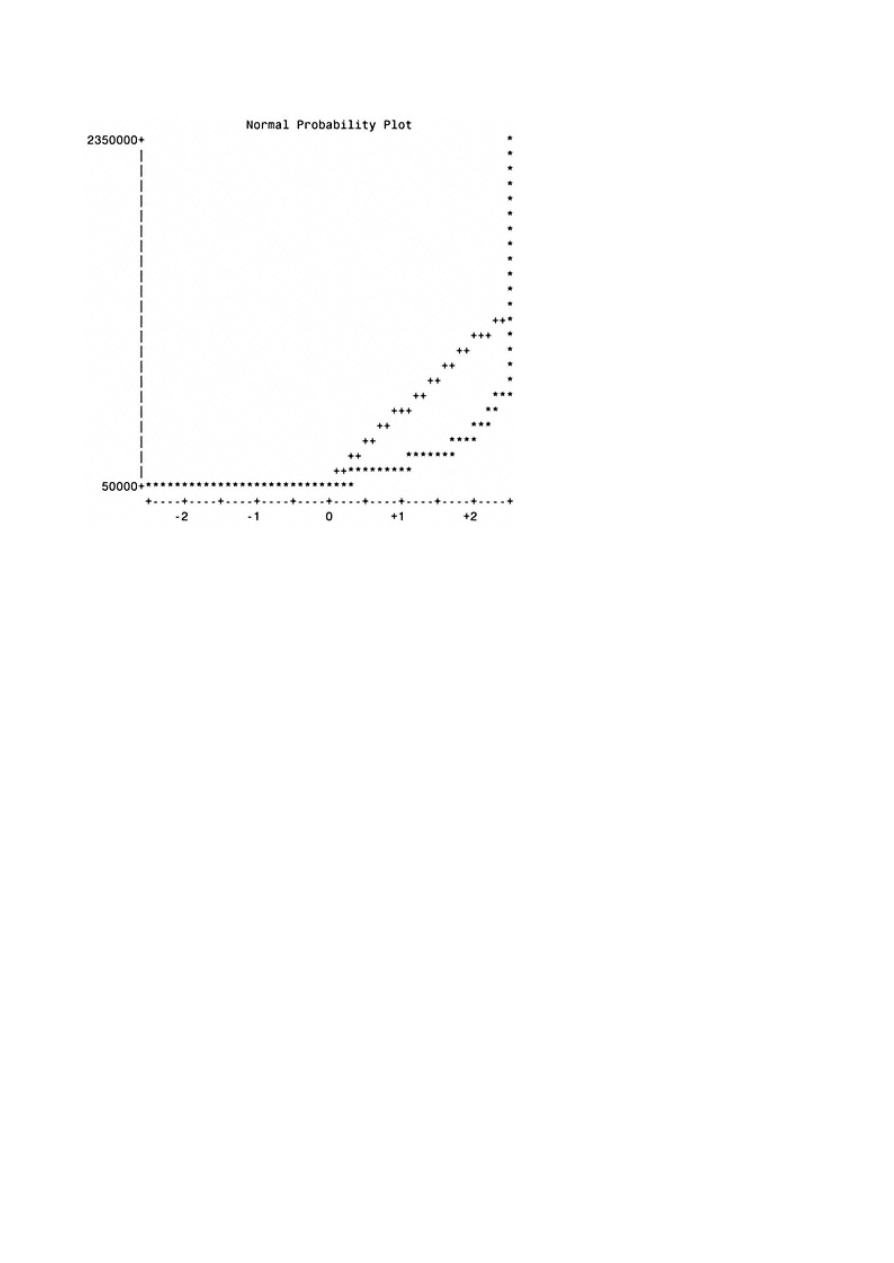
Page 325

Inferred Age

Univariate Procedure

Variable=INFD_AG
Weight= SMP_WGT

Moments

85404

Sum Wgts

729228

Mean

42.83768

Sum

31238435

Std Dev

27.21078

Variance

740.4265

Skewness

Kurtosis

USS

1.4014E9

CSS

63234643

63.52067

Std Mean

0.031865

T:Mean=0

1344.363

Pr>|T|

0.0001

Num ^= 0

85404

Num > 0

85404

M(Sign)

42702

Pr>=|M|

0.0001

Sgn Rank

1.8235E9

Pr>=|S|

0.0001

Page 326

Quantiles (Def=5)

100% Max

99%

75% Q3

95%

50% Med

90%

25% Q1

10%

0% Min

Range

Q3-Q1

Mode

Extremes

Lowest

Obs

Highest

Obs

25(

85399)

65(

84255)

25(

85395)

65(

84326)

25(

85390)

65(

84334)

25(

85383)

65(

85187)

25(

85372)

65(

85368)

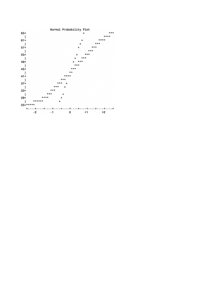
Page 327

Total Accounts

Univariate Procedure

Variable=TOT_ACC
Weight= SMP_WGT

Moments

85404

Sum Wgts

729228

Mean

19.96658

Sum

14560189

Std Dev

32.37958

Variance

1048.437

Skewness

Kurtosis

USS

3.8026E8

CSS

89539683

162.1689

Std Mean

0.037917

T:Mean=0

526.5797

Pr>|T|

0.0001

Num ^= 0

85404

Num > 0

85404

M(Sign)

42702

Pr>=|M|

0.0001

Sgn Rank

1.8235E9

Pr>=|S|

0.0001

Page 328

Quantiles (Def=5)

100% Max

99%

75% Q3

95%

50% Med

90%

25% Q1

10%

0% Min

Range

Q3-Q1

Mode

Extremes

Lowest

Obs

Highest

Obs

76936)

76(

521)

75718)

77(

77634)

74479)

78(

684)

72540)

78(

69582)

72152)

87(

47533)

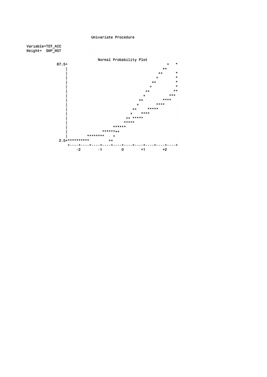
Page 329

Accounts Open in Last 6 Months

Univariate Procedure

Variable=ACTOPL6
Weight= SMP_WGT

Moments

85404

Sum Wgts

729228

Mean

1.153018

Sum

840813

Std Dev

3.209506

Variance

10.30093

Skewness

Kurtosis

USS

1849203

CSS

879730.5

278.357

Std Mean

0.003758

T:Mean=0

306.7817

Pr>|T|

0.0001

Num ^= 0

60711

Num > 0

60711

M(Sign)

30355.5

Pr>=|M|

0.0001

Sgn Rank

9.2147E8

Pr>=|S|

0.0001

Page 330

Quantiles (Def=5)

100% Max

99%

75% Q3

95%

50% Med

90%

25% Q1

10%

0% Min

Range

Q3-Q1

Mode

Extremes

Lowest

Obs

Highest

Obs

85404)

11(

41050)

85401)

12(

56381)

85394)

13(

64495)

85388)

14(

23611)

85384)

16(

18716)

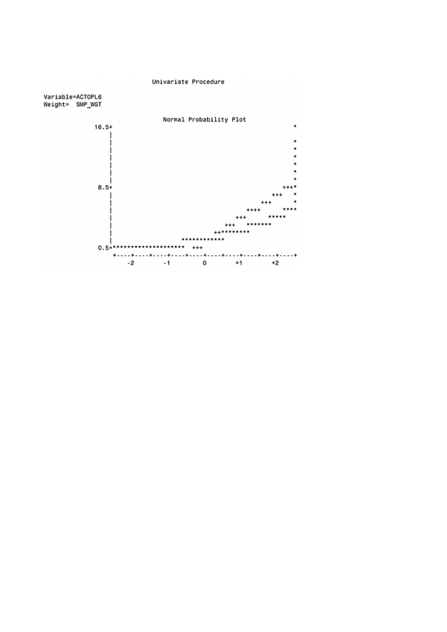
Page 331

Evaluation of actopl6

Total Balances

Univariate Procedure

Variable=TOT_BAL
Weight= SMP_WGT

Moments

85404

Sum Wgts

729228

Mean

129490.5

Sum

9.443E10

Std Dev

504678.2

Variance

2.547E11

Skewness

Kurtosis

USS

3.398E16

CSS

2.175E16

389.7416

Std Mean

590.9937

T:Mean=0

219.1063

Pr>|T|

0.0001

Num ^= 0

83616

Num > 0

83616

M(Sign)

41808

Pr>=|M|

0.0001

Sgn Rank

1.7479E9

Pr>=|S|

0.0001

Page 332

Quantiles (Def=5)

100% Max

5544774

99%

741006

75% Q3

182987

95%

399898

50% Med

79779

90%

298176

25% Q1

10690.5

10%

1096

0% Min

261

Range

5544774

Q3-Q1

172296.5

Mode

Extremes

Lowest

Obs

Highest

Obs

85280)

3983490(

40154)

85133)

4102490(

23869)

84961)

4163294(

19189)

84873)

4701462(

69915)

84835)

5544774(

17281)

Team-Fly

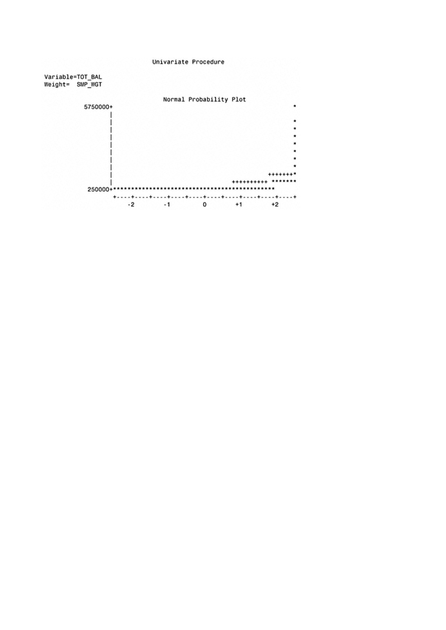
Page 333

Number of Inquiries in Last 6 Months

Univariate Procedure

Variable=INQL6M
Weight= SMP_WGT

Moments

85404

Sum Wgts

729228

Mean

0.903981

Sum

659208

Std Dev

3.9358 Variance

15.49052

Skewness

Kurtosis

USS

1918848

CSS

1322937

435.3854

Std Mean

0.004609

T:Mean=0

196.1362

Pr>|T|

0.0001

Num ^= 0

41183

Num > 0

41183

M(Sign)

20591.5

Pr>=|M|

0.0001

Sgn Rank

4.2402E8

Pr>=|S|

Quantiles (Def=5)

100% Max

99%

75% Q3

95%

50% Med

90%

25% Q1

10%

0% Min

Range

Q3-Q1

Mode

Page 334

Extremes

Lowest

Obs

Highest

Obs

85402)

16(

28580)

85401)

17(

58346)

85400)

18(

9388)

85399)

18(

56381)

85398)

22(

41413)

Page 335

Total Open Accounts

Univariate Procedure

Variable=TOTOPAC
Weight= SMP_WGT

Moments

85404

Sum Wgts

729228

Mean

12.57202

Sum

9167868

Std Dev

20.34971

Variance

414.1109

Skewness

Kurtosis

USS

1.5062E8

CSS

35366311

161.8651

Std Mean

0.02383

T:Mean=0

527.5679

Pr>|T|

0.0001

Num ^= 0

85404

Num > 0

85404

M(Sign)

42702

Pr>=|M|

0.0001

Sgn Rank

1.8235E9

Pr>=|S|

0.0001

Page 336

Quantiles (Def=5)

100% Max

99%

75% Q3

95%

50% Med

90%

25% Q1

10%

0% Min

Range

Q3-Q1

Mode

Extremes

Lowest

Obs

Highest

Obs

85290)

54(

56001)

85068)

57(

25775)

84622)

57(

56381)

84417)

59(

69582)

84246)

63(

684)

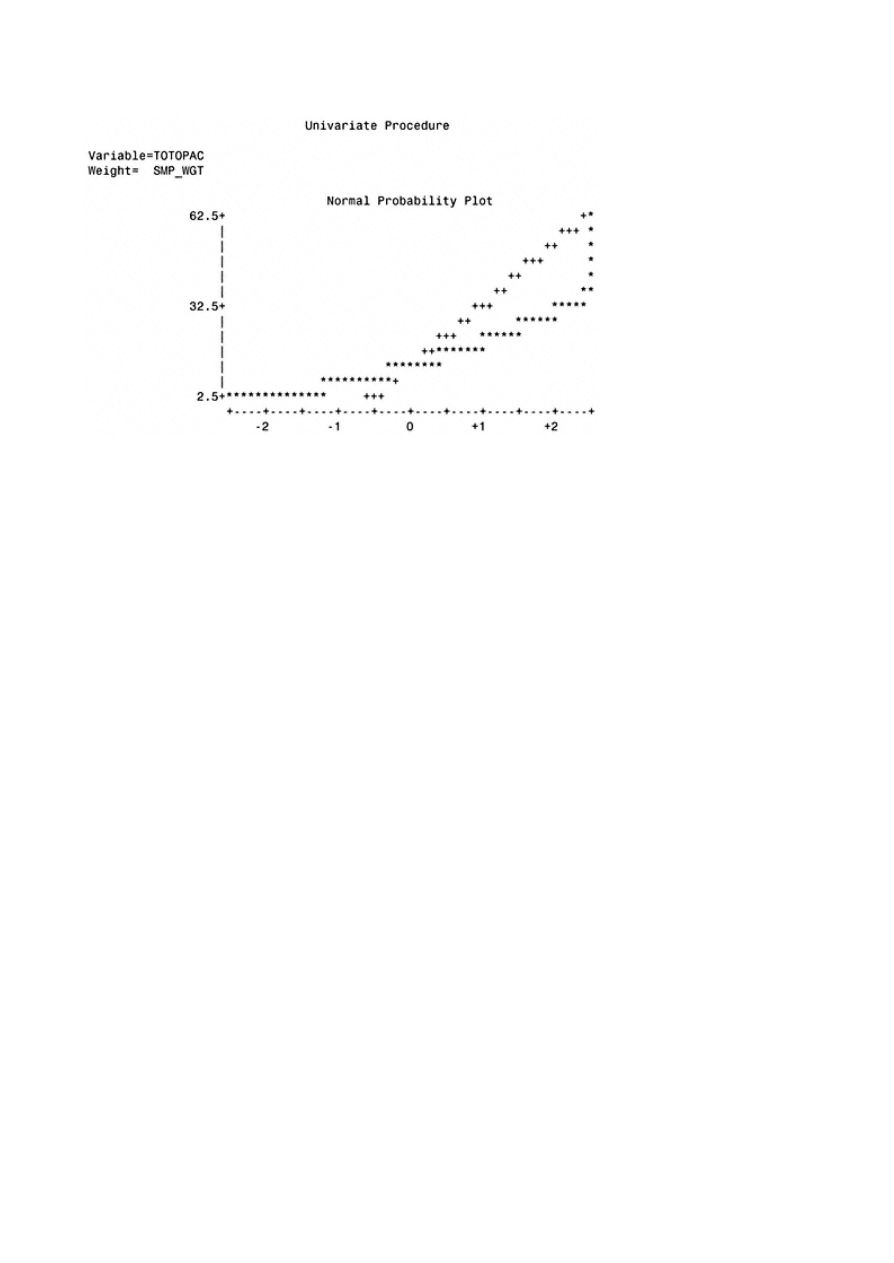
Page 337

Total Credit Lines

Univariate Procedure

Variable=CREDLIN
Weight= SMP_WGT

Moments

85404

Sum Wgts

729228

Mean

173929

Sum

1.268E11

Std Dev

581723.2

Variance

3.384E11

Skewness

Kurtosis

USS

5.096E16

CSS

2.89E16

334.4601

Std Mean

681.2158

T:Mean=0

255.3215

Pr>|T|

0.0001

Num ^= 0

85366

Num > 0

85366

M(Sign)

42683

Pr>=|M|

0.0001

Sgn Rank

1.8219E9

Pr>=|S|

0.0001

Quantiles (Def=5)

100% Max

9250120

99%

867178

75% Q3

237600

95%

488500

50% Med

123900

90%

370506

25% Q1

35445

10%

14610

0% Min

7500

1159

Range

9250120

Q3-Q1

202155

Mode

10000

Page 338

Extremes

Lowest

Obs

Highest

Obs

84821)

4577900(

23869)

79629)

4828676(

19189)

74719)

5451884(

69915)

70318)

5745300(

17281)

59675)

9250120(

13742)

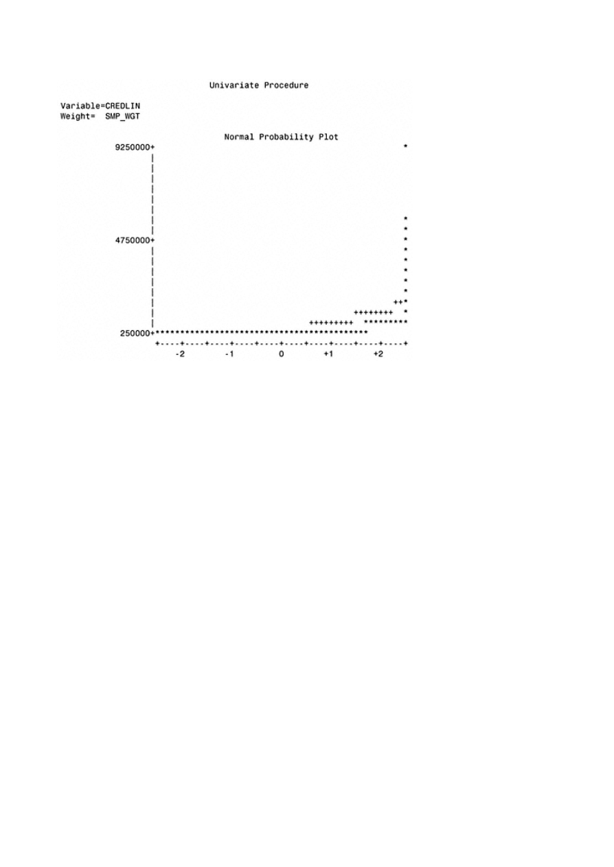
Page 339

Age of File

Univariate Procedure

Variable=AGE_FIL
Weight= SMP_WGT

Moments

85404

Sum Wgts

729228

Mean

174.3028

Sum

1.2711E8

Std Dev

254.3212

Variance

64679.28

Skewness

Kurtosis

USS

2.768E10

CSS

5.5238E9

145.9077

Std Mean

0.297818

T:Mean=0

585.2661

Pr>|T|

0.0001

Num ^= 0

85351

Num > 0

85351

M(Sign)

42675.5

Pr>=|M|

0.0001

Sgn Rank

1.8212E9

Pr>=|S|

0.0001

Page 340

Quantiles (Def=5)

100% Max

666

99%

347

75% Q3

227

95%

329

50% Med

169

90%

295

25% Q1

108

10%

0% Min

Range

666

Q3-Q1

119

Mode

214

Extremes

Lowest

Obs

Highest

Obs

84242)

619(

84665)

81481)

625(

58765)

80706)

663(

38006)

80589)

666(

10497)

76936)

666(

71596)

Team-Fly

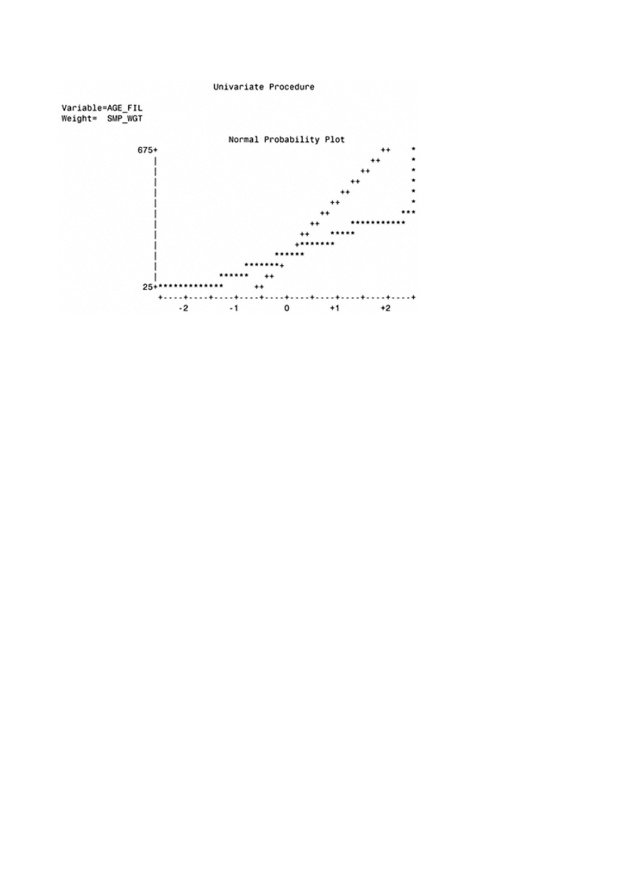
Page 341

Number of 30 -Day Delinquencies

Univariate Procedure

Variable=NO30DAY
Weight= SMP_WGT

Moments

85404

Sum Wgts

729228

Mean

0.718138

Sum

523686

Std Dev

5.898548

Variance

34.79287

Skewness

Kurtosis

USS

3347494

CSS

2971415

821.3675

Std Mean

0.006907

T:Mean=0

103.9667

Pr>|T|

0.0001

Num ^= 0

22303

Num > 0

22303

M(Sign)

11151.5

Pr>=|M|

0.0001

Sgn Rank

1.2436E8

Pr>=|S|

0.0001

Page 342

Quantiles (Def=5)

100% Max

99%

75% Q3

95%

50% Med

90%

25% Q1

10%

0% Min

Range

Q3-Q1

Mode

Extremes

Lowest

Obs

Highest

Obs

85404)

37(

78590)

85403)

38(

44354)

85402)

38(

47412)

85401)

43(

7285)

85400)

43(

46812)

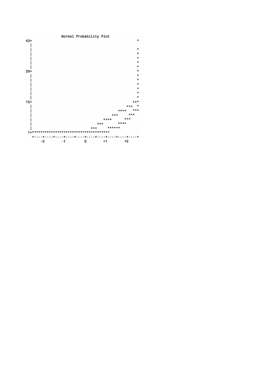
Page 343

Replacing Missing Values for Income

The first frequency shows the distribution of HOME EQUITY. This is used to create the matrix that displays the mean
INCOME by HOME EQUITY range and AGE Group.

HOMEQ_R

Frequency

Percent

Cumulative

Frequency

Cumulative

Percent

$0-$100K

53723

62.9

53723

62.9

$100-$20

20285

23.8

74008

86.7

$200-$30

7248

8.5

81256

95.1

$300-$40

2269

2.7

83525

97.8

$400-$50

737

0.9

84262

98.7

$500-$60

339

0.4

84601

99.1

$600-$70

213

0.2

84814

99.3

$700K+

590

0.7

85404

100.0

Mean INCOME by HOME EQUITY and AGE Group

Age group

25-34

35-44

45-54

55-65

Home Equity

$47

$55

$57

$55

$0-$100K

$100-$20

$70

$73

$72

$68

$200-$30

$66

$73

$76

$68

$300-$40

$70

$80

$84

$76

$400-$50

$89

$93

$94

$93

$500-$60

$98

$101

$102

$97

$600-$70

$91

$105

$109

$104

$700K+

$71

$102

$111

$107

The following regression used INFERRED AGE, HOME EQUITY, CREDIT LINE and TOTAL BALANCES to predict missing values for
INCOME.

Step 0

All Variables Entered R-square = 0.66962678

C(p) = 5.000000000

Sum of Squares

Mean Square

Regression

372912001.28200

93228000.320499

43230.8

Error

85315

183983294.99609

2156.51755255

Total

85319

556895296.27809

Parameter

Standard

Type II

Variable

Estimate

Error

Sum of Squares

INTERCEP

36.87607683

0.25721498

44325117.661102

20554.0

INFD_AGE2

0.11445815

0.00602800

777500.06857066

360.54

HOM_EQU2

-0.00000343

0.00000040

158246.95496857

73.38

CREDLIN2

0.00011957

0.00000120

21410199.091371

9928.14

TOT_BAL2

-0.00000670

0.00000136

52180.72203473

24.20

Bounds on condition number:

19.28444,

161.5108

Page 345

All variables left in the model are significant at the 0.1000 level.

OBS _MODEL_ _TYPE_ _DEPVAR_ _RMSE_ INTERCEP INFD_AG2

1 INC_REG PARMS INC_EST2 46.4383 36.8761 0.11446

OBS HOM_EQU2 CREDLIN2 TOT_BAL2 INC_EST2

1 -.0000034348 .00011957 -.0000067044 -1

The following print output displays the values for INCOME after regression substitution.

OBS

INC_EST2

INC_EST3

436

43.3210

2027

44.5382

4662

40.2160

5074

43.5390

5256

41.6833

5552

43.1713

6816

41.4527

8663

62.8130

10832

42.3638

11052

42.4500

14500

41.6961

14809

41.2255

15132

63.4676

15917

41.2685

16382

41.8029

16788

40.8224

16832

34.2062

16903

42.0813

17201

43.5734

17419

42.8501

17540

43.9865

17700

40.3016

18045

42.4653

18147

43.5607

18254

41.3758

18296

41.3878

18362

41.5944

18597

40.7010

18931

51.3921

19058

42.4845

20419

42.0720

20640

40.1936

22749

42.1277

23201

42.6050

23334

42.4007

23651

41.7607

24227

34.0227

24764

39.8351

25759

42.0662

continues

Page 346

(Continued)

OBS

INC_EST2

INC_EST3

26608

54.4467

30922

42.8928

31141

41.6508

32963

42.6343

32986

41.2255

34175

41.2114

34702

41.6541

35897

47.0708

36616

42.7077

42978

41.3285

44612

53.0752

45165

43.7436

45959

41.1110

46242

41.9122

46428

41.6833

46439

42.5990

47002

42.0267

47400

41.8678

48237

51.3944

49472

44.1610

50012

41.7293

50059

43.1998

50236

42.3850

50446

42.0642

51312

42.6312

52741

42.0676

53961

42.1993

53972

43.8084

54715

43.3766

55422

44.0192

57848

45.8676

59262

41.3399

59450

41.4544

59512

43.7946

59675

41.4544

60545

46.7328

64254

52.3536

66336

42.3752

69200

43.4159

70318

41.5689

72152

41.6255

72540

42.5443

74479

42.8142

75718

42.3963

76936

42.8469

Page 347

APPENDIX B—
UNIVARIATE ANALYSIS OF CATEGORICAL VARIABLES

In this appendix you will find simple frequencies of the categorical variables discussed in chapter 3.

Categorical Variables

POP_DEN

Frequency

Percent

Cumulative

Frequency

Cumulative

Percent

143889

19.7

143889

19.7

46934

6.4

190823

26.2

267947

36.7

458770

62.9

270458

37.1

729228

100.0

TRAV_CD

Frequency

Percent

Cumulative

Frequency

Cumulative

Percent

220060

30.2

220060

30.2

509168

69.8

729228

100.0

BANKCRD

Frequency

Percent

Cumulative

Frequency

Cumulative

Percent

40817

5.6

40817

5.6

688411

94.4

729228

100.0

APT_IND

Frequency

Percent

Cumulative

Frequency

Cumulative

Percent

600369

82.3

600369

82.3

128859

17.7

729228

100.0

(table continued on next page)

Page 348

(table continued from previous page)

Categorical Variables

CLUSTR1

Frequency

Percent

Cumulative
Frequency

Cumulative
Percent

594

0.1

594

0.1

1854

0.3

2448

0.3

947

0.1

3395

0.5

2278

0.3

5673

0.8

2269

0.3

7942

1.1

1573

0.2

9515

1.3

1306

0.2

10821

1.5

1668

0.2

12489

1.7

1120

0.2

13609

1.9

2518

0.3

16127

2.2

5759

0.8

21886

3.0

404

0.1

22290

3.1

1194

0.2

23484

3.2

59097

8.1

82581

11.3

7114

1.0

89695

12.3

8268

1.1

97963

13.4

14128

1.9

112091

15.4

1614

0.2

113705

15.6

1091

0.1

114796

15.7

13479

1.8

128275

17.6

7695

1.1

135970

18.6

3808

0.5

139778

19.2

878

0.1

140656

19.3

1408

0.2

142064

19.5

1272

0.2

143336

19.7

5459

0.7

148795

20.4

28935

4.0

177730

24.4

33544

4.6

211274

29.0

14517

2.0

225791

31.0

3862

0.5

229653

31.5

0.0

229694

31.5

153

0.0

229847

31.5

1550

0.2

231397

31.7

Team-Fly

1321

0.2

232718

31.9

1757

0.2

234475

32.2

121832

16.7

356307

48.9

24836

3.4

381143

52.3

29429

4.0

410572

56.3

6902

0.9

417474

57.2

65318

9.0

482792

66.2

180767

24.8

663559

91.0

65669

9.0

729228

100.0

(table continued on next page)

Page 349

(table continued from previous page)

Categorical Variables

INC_GRP

Frequency

Percent

Cumulative

Frequency

Cumulative

Percent

750

0.1

750

0.1

566

0.1

1316

0.2

12040

1.7

13356

1.8

41007

5.6

54363

7.5

64095

8.8

118458

16.2

82088

11.3

200546

27.5

62449

8.6

262995

36.1

47412

6.5

310407

42.6

40136

5.5

350543

48.1

41641

5.7

392184

53.8

43885

6.0

436069

59.8

43091

5.9

479160

65.7

40647

5.6

519807

71.3

35647

4.9

555454

76.2

30169

4.1

585623

80.3

24702

3.4

610325

83.7

20056

2.8

630381

86.4

17819

2.4

648200

88.9

81028

11.1

729228

100.0

SGLE_IN

Frequency

Percent

Cumulative

Frequency

Cumulative

Percent

627089

86.0

627089

86.0

102139

14.0

729228

100.0

FINL_ID

Frequency

Percent

Cumulative

Frequency

Cumulative

Percent

24293

3.3

24293

3.3

11908

1.6

36201

5.0

693027

95.0

729228

100.0

HH_IND

Frequency

Percent

Cumulative

Frequency

Cumulative

Percent

119833

16.4

119833

16.4

609395

83.6

729228

100.0

GENDER

Frequency

Percent

Cumulative

Frequency

Cumulative

Percent

293331

40.2

293331

40.2

124038

17.0

417369

57.2

311859

42.8

729228

100.0

(table continued on next page)

Page 350

(table continued from previous page)

Categorical Variables

SSN_IND

Frequency

Percent

Cumulative

Frequency

Cumulative

Percent

283

0.0

283

0.0

728945

100.0

729228

100.0

DRIV_IN

Frequency

Percent

Cumulative

Frequency

Cumulative

Percent

338410

46.4

338410

46.4

333066

45.7

671476

92.1

57752

7.9

729228

100.0

MOB_IND

Frequency

Percent

Cumulative

Frequency

Cumulative

Percent

437608

60.0

437608

60.0

246167

33.8

683775

93.8

45453

6.2

729228

100.0

MORTIN1

Frequency

Percent

Cumulative

Frequency

Cumulative

Percent

163498

22.4

163498

22.4

185182

25.4

348680

47.8

78226

10.7

426906

58.5

302322

41.5

729228

100.0

MORTIN2

Frequency

Percent

Cumulative

Frequency

Cumulative

Percent

322189

44.2

322189

44.2

87986

12.1

410175

56.2

175422

24.1

585597

80.3

143631

19.7

729228

100.0

AUTOIN1

Frequency

Percent

Cumulative

Frequency

Cumulative

Percent

261487

35.9

261487

35.9

135457

18.6

396944

54.4

127951

17.5

524895

72.0

204333

28.0

729228

100.0

(table continued on next page)

Page 351

(table continued from previous page)

Categorical Variables

AUTOIN2

Frequency

Percent

Cumulative

Frequency

Cumulative

Percent

386914

53.1

386914

53.1

57109

7.8

444023

60.9

206299

28.3

650322

89.2

78906

10.8

729228

100.0

INFD_AG

Frequency

Percent

Cumulative

Frequency

Cumulative

Percent

13682

1.9

13682

1.9

11819

1.6

25501

3.5

11137

1.5

36638

5.0

12633

1.7

49271

6.8

12336

1.7

61607

8.4

12522

1.7

74129

10.2

15535

2.1

89664

12.3

15653

2.1

105317

14.4

17603

2.4

122920

16.9

18485

2.5

141405

19.4

20648

2.8

162053

22.2

27641

3.8

189694

26.0

29476

4.0

219170

30.1

30475

4.2

249645

34.2

33801

4.6

283446

38.9

32400

4.4

315846

43.3

28286

3.9

344132

47.2

27794

3.8

371926

51.0

26004

3.6

397930

54.6

26421

3.6

424351

58.2

21694

3.0

446045

61.2

24183

3.3

470228

64.5

24773

3.4

495001

67.9

24662

3.4

519663

71.3

24190

3.3

543853

74.6

25831

3.5

569684

78.1

22334

3.1

592018

81.2

19074

2.6

611092

83.8

16752

2.3

627844

86.1

16067

2.2

643911

88.3

15032

2.1

658943

90.4

10454

1.4

669397

91.8

9350

1.3

678747

93.1

8349

1.1

687096

94.2

7780

1.1

694876

95.3

8172

1.1

703048

96.4

7487

1.0

710535

97.4

5336

0.7

715871

98.2

4489

0.6

720360

98.8

4486

0.6

724846

99.4

4382

0.6

729228

100.0

(table continued on next page)

Page 352

(table continued from previous page)

AGE_IND

Frequency

Percent

Cumulative

Frequency

Cumulative

Percent

204132

28.0

204132

28.0

525096

72.0

729228

100.0

Categorical Variables

DOB_YR

Frequency

Percent

Cumulative

Frequency

Cumulative

Percent

0000

193460

26.5

193460

26.5

1900

10672

1.5

204132

28.0

1933

4382

0.6

208514

28.6

1934

4486

0.6

213000

29.2

1935

4489

0.6

217489

29.8

1936

5205

0.7

222694

30.5

1937

5074

0.7

227768

31.2

1938

5203

0.7

232971

31.9

1939

5264

0.7

238235

32.7

1940

5668

0.8

243903

33.4

1941

6100

0.8

250003

34.3

1942

7242

1.0

257245

35.3

1943

11260

1.5

268505

36.8

1944

12115

1.7

280620

38.5

1945

12240

1.7

292860

40.2

1946

14302

2.0

307162

42.1

1947

16127

2.2

323289

44.3

1948

15912

2.2

339201

46.5

1949

16367

2.2

355568

48.8

1950

16709

2.3

372277

51.1

1951

17097

2.3

389374

53.4

1952

16767

2.3

406141

55.7

1953

17725

2.4

423866

58.1

1954

18232

2.5

442098

60.6

1955

18541

2.5

460639

63.2

1956

18244

2.5

478883

65.7

1957

19008

2.6

497891

68.3

1958

19885

2.7

517776

71.0

1959

19833

2.7

537609

73.7

1960

18873

2.6

556482

76.3

1961

18967

2.6

575449

78.9

1962

18945

2.6

594394

81.5

1963

17876

2.5

612270

84.0

1964

16903

2.3

629173

86.3

1965

15641

2.1

644814

88.4

1966

14213

1.9

659027

90.4

1967

13757

1.9

672784

92.3

1968

11442

1.6

684226

93.8

1969

10731

1.5

694957

95.3

1970

10476

1.4

705433

96.7

1971

8726

1.2

714159

97.9

1972

7703

1.1

721862

99.0

1973

7366

1.0

729228

100.0

(table continued on next page)

Page 353

(table continued from previous page)

HOMEQ_R

Frequency

Percent

Cumulative

Frequency

Cumulative

Percent

$0-$100K

449255

61.6

449255

61.6

$100-$20

178739

24.5

627994

86.1

$200-$30

64218

8.8

692212

94.9

$300-$40

20089

2.8

712301

97.7

$400-$50

6650

0.9

718951

98.6

$500-$60

3003

0.4

721954

99.0

$600-$70

1932

0.3

723886

99.3

$700K+

5342

0.7

729228

100.0

Categorical Variables

CHILDIN

Frequency

Percent

Cumulative

Frequency

Cumulative

Percent

577499

79.2

577499

79.2

151729

20.8

729228

100.0

HOMEVLR

Frequency

Percent

Cumulative

Frequency

Cumulative

Percent

239556

32.9

239556

32.9

0.0

239607

32.9

2135

0.3

241742

33.2

12731

1.7

254473

34.9

30353

4.2

284826

39.1

45397

6.2

330223

45.3

52762

7.2

382985

52.5

53632

7.4

436617

59.9

48610

6.7

485227

66.5

42960

5.9

528187

72.4

35313

4.8

563500

77.3

53132

7.3

616632

84.6

34544

4.7

651176

89.3

21226

2.9

672402

92.2

14080

1.9

686482

94.1

15300

2.1

701782

96.2

8364

1.1

710146

97.4

5114

0.7

715260

98.1

3317

0.5

718577

98.5

2340

0.3

720917

98.9

8311

1.1

729228

100.0

(table continued on next page)

Team-Fly

Page 354

(table continued from previous page)

CLUSTR2

Frequency

Percent

Cumulative

Frequency

Cumulative

Percent

698544

95.8

698544

95.8

2138

0.3

700682

96.1

1765

0.2

702447

96.3

795

0.1

703242

96.4

1999

0.3

705241

96.7

9784

1.3

715025

98.1

6651

0.9

721676

99.0

4710

0.6

726386

99.6

2842

0.4

729228

100.0

Page 355

RECOMMENDED READING

Berry, Michael J.A., and Gordon Linoff. 1997. Data Mining Techniques. New York: John Wiley & Sons.

Berry, Michael J.A., and Gordon Linoff. 1997. Mastering Data Mining. New York: John Wiley & Sons.

Hosmer, David W., and Stanley Lemeshow. 1989. Applied Logistic Regression. New York: John Wiley &
Sons.

Hughes, Arthur M. 1994. Strategic Database Marketing . Chicago: Probus Publishing.

Journal of Targeting, Measurement and Analysis for Marketing. London: Henry Stewart
Publications.

Tukey, John W. 1977. Exploratory Data Analysis . Reading, MA: Addison-Wesley.

Page 357

WHAT'S ON THE CD-ROM?

The CD -ROM contains step-by -step instructions for developing the data models described in Data Mining Cookbook.
Written in SAS code, you can use the contents as a template to create your own models. The content on the CD -ROM is
equivalent to taking a three-day course in data modeling.

The CD -ROM includes full examples of all the code necessary to develop a variety of models including response,
approval, attrition or churn, risk, and lifetime or net present value. Detailed code for developing the objective function
includes examples from the credit cards, insurance, telecommunications, and catalog industries. The code is well
documented and explains the goals and methodology for each step. The only software needed is BASE SAS and
SAS/STAT. The spreadsheets used for creating gains tables and lift charts are also included. These can be used by
plugging in the preliminary results from the analyses created in SAS. While the steps before and after the model
processing can be used in conjunction with any data modeling software package, the code can also serve as a stand-alone
modeling template. The model processing steps focus on variable preparation for use in logistic regression. Additional
efficiencies in the form of SAS macros for variable processing and validation are included.

Page 358

Hardware Requirements

To use this CD-ROM, your system must meet the following requirements:

Platform/processor/operating system: Windows® 95, NT 4.0 or higher; 200 MHz
Pentium

RAM: 64 MB minimum; 128 MB recommended

Hard drive space: Nothing will install to the hard drive, but in order to make a local copy of all the files on the CD-
ROM requires 5 MB of free space.

Peripherals: CD-ROM drive. You also will need to have the following applications to make full use of the CD-ROM: a
running copy of SAS 6.12 or higher software to process SAS code provided; a browser such as Internet Explorer or
Netscape Navigator to navigate the CD-ROM; Microsoft Excel 97/2000 or Microsoft Excel 5.0/95.

Installing the Software

Insert the CD-ROM and launch the readme.htm file in a web browser, or navigate using Windows Explorer to browse
the contents of the CD. The model programs and output are in text format that can be opened in any editing software
(including SAS) that reads ASCII files. Spreadsheets are in Microsoft Excel 97/2000 and Microsoft Excel 5.0/95.
Launch the application (SAS 6.12 or higher) and open the file directly from the CD-ROM. If you wish to make changes,
you can rename the files and save them to your local hard drive.

Using the Software

The CD is organized into folders that correspond to each chapter in Data Mining Cookbook. Within each folder are sub-
folders containing SAS programs, SAS output, Excel spreadsheets. The programs can be used as templates. You just
need to change the data set and variable names. More specific instructions on how to use the programs are included. The
output is included to provide a more complete understanding of the recipes in Data Mining Cookbook. The spreadsheets
contain all formulas used to create the tables and charts in Data Mining Cookbook.

Page 359

INDEX

Access log,

307

309

Accessing the data,

–57

ASCII and,

–53

classifying data,

–55

reading raw data,

–57

Activation models,

Adaptive company,

–23

hiring and teamwork,

–22

product focus versus customer focus,

–23

American Standard for Computer Information Interchange. See ASCII files

Analyst

hiring of,

retaining,

teamwork with,

Analytics. See Adaptive company

Approval models. See Risk models

ASCII files,

access log and,

307

codes for,

fixed format,

–53

variable format,

Attitudinal data,

–27

Attrition,

–11.

See also Modeling churn

case example of,

credit cards and silent type of,

258

defining to optimize profits,

259

–261

definition of,

opportunities by industry,

profile creation of,

273

274

–275

Auditing and scoring outside,

155

–161

Back-end validation,

176

–177

Backward regression,

103

105

109

–110,

112

221

222

245

268

Bad data,

175

Balance bombs,

201

Bayes' Theorem,

121

Behavioral data,

Bootstrapping,

138

140

–146,

147

148

adjusting,

146

analysis,

229

churn modeling and,

270

271

272

–273

formula for,

140

jackknifing versus,

138

validation using,

138

140

–146,

147

148

224

225

227

–230,

249

251

270

Branding on the Web,

316

–317

Business builders customers,

201

Business intelligence infrastructure,

Categorical variables,

–70,

–85,

218

–220

churn modeling and,

265

266

–268

linear predictors development and,

–97

Champion versus challenger,

166

–167,

175

Chi-square statistic,

247

backward regression and,

105

categorical variables and,

218

–219

continuous variables and,

210

–211

forward selection method and,

104

score selection method and,

105

Page 360

(continued)

Chi-square statistic

stepwise regression and,

105

variable reduction and,

Churn,

See also Modeling churn (retaining profitable customers)

case example of,

definition of,

Classification trees,

–20

example of,

goal of,

interaction detection using,

linear regression versus,

purpose of,

software for building,

Classifying data,

–55

qualitative,

quantitative,

Cleaning the data,

–70,

188

categorical variables,

–70

continuous variables,

–69

missing values,

–69

outliers and data errors,

–64

Web and,

309

Cluster analysis,

184

example,

205

–206

performing to discover customer segments,

203

–204,

205

–206

Collaborative filtering on the Web,

313

–316

ad targeting,

315

applications in near future,

315

call centers,

315

e-commerce,

315

of information,

313

knowledge management and,

314

managing personal resources,

316

marketing campaigns,

315

trend in evolution of,

314

workings of,

–10

Combining data from multiple offers,

–48

Computers

logistic models and,

Constructing modeling data set,

–48

combining data from multiple offers,

–48

developing models from modeled data,

sample size,

–45

sampling methods,

–47

Consummate consumers,

201

Continuous data,

–55

Continuous variables,

–79,

157

210

–218,

236

churn modeling and,

263

–265,

266

means analysis of,

212

transformation of,

215

–216,

267

Cookie,

308

Cooking demonstration,

–180

implementing and maintaining model,

151

–180

preparing data for modeling,

–70

processing and evaluating model,

101

–124

selecting and transforming variables,

–99

validating model,

125

–150

Creating modeling data set,

–59

sampling,

–59

Credit bureaus,

Credit scoring and risk modeling,

232

–233

Cross-sell model,

case example of,

opportunities for,

Customer, understanding your,

183

–206

cluster analysis performing to discover customer segments,

203

–204,

205

–206

developing customer value matrix for credit card company,

198

–203

importance of,

184

–189

market segmentation keys,

186

–189

profiling and penetration analysis of catalog company's customers,

190

–198

summary of,

204

types of profiling and segmentation,

184

–186

value analysis,

109

–203

Customer acquisition modeling examples,

–40

Page 361

Customer database components,

–29

Customer focus versus product focus,

–23

Customer insight gaining in real time,

317

–318

Customer loyalty,

258

Customer models, data for,

–42

Customer profitability optimizing,

276

–278

Customer relationship management (CRM),

284

285

286

Customer value matrix development,

198

–203

Data

types of,

–27

validation,

152

–155

Data errors and outliers,

–64,

Data marts,

Data mining software classification trees,

Data preparation for modeling. See Preparing data for modeling

Data requirements review and evaluation,

187

–188

Data sources selecting,

–48

constructing modeling data set,

–48

for modeling,

–44

sources of data,

–36

summary of,

types of data,

–27

Data warehouse,

–35

definition of,

meta data role,

mistakes and best practices,

–35

typical,

Dates,

–76

Decile analysis,

101

247

297

bootstrapping and,

140

–141

calculating,

239

Team-Fly

creating,

113

116

–117,

122

–123

example,

249

file cut-off determination and,

166

gains table and,

149

on key variables,

146

–150

of scored file,

164

using validation data,

118

120

121

123

Decision tree. See Classification trees

Demographic data,

characteristics of,

Demographics and profile analysis,

–8,

185

–186

Descriptive models,

Developing models from modeled data,

Duration and lifetime value modeling,

284

285

–286

E-mail inquiry on response data,

308

Evaluating and processing the model. See Processing and evaluating the model

Exploratory data analysis,

175

External validity of model,

174

Factor analysis,

184

File cut-off determination,

166

Financials, calculating,

161

–165

Focus on product versus customer,

–23

Fraud,

253

254

–255

Frequency type of profiling,

185

Gains tables and charts,

125

–129

creating,

126

–127,

247

examples,

126

129

133

138

139

145

147

149

lifetime value model and,

301

302

303

304

NPV model,

165

for score comparison,

250

two model method and,

127

–129

validation examples,

128

129

226

–227,

271

272

Genetic algorithms,

–18

example,

Goal defining,

–12

activation,

Page 362

(continued)

Goal defining

attrition,

–11

cross-sell and up-sell,

lifetime value,

–12

net present value,

profile analysis,

–8

response,

–9

risk,

–10

segmentation,

steps in,

High-risk customers, avoiding,

231

–255. See also Modeling risk

Hiring and teamwork,

–22

Implementing and maintaining the model,

151

–180,

230

back-end validation,

176

–177

calculating the financials,

161

–165

champion versus challenger,

166

–167

checking,

172

churn and,

273

–278

determining file cut-off,

166

high-risk customer avoidance and,

251

–253

maintenance,

177

–179

scoring a new file,

151

–161

summary of,

179

–180

tracking,

170

–177

two-model matrix,

167

–170

Intelligence architecture of business,

Interactions detection,

–99

Internal validity of model,

174

Interval data,

Jackknifing,

134

–138,

139

Lifecycle of model,

175

177

–178

benchmarking,

177

rebuild or refresh,

177

–178

Life stage as type of profiling,

186

Lifetime value model,

–12,

281

–304. See also Modeling lifetime value

Lift measurement,

127

136

137

141

143

224

225

226

Linear predictors development,

–97

categorical variables,

–97

continuous variables,

–95

Linear regression analysis,

–14,

208

209

295

examples,

logistic regression versus,

net revenues and,

292

neural networks versus,

List compilers,

List fatigue,

173

–174

List sellers,

Logistic regression,

–4,

295

296

categorical variables and,

218

continuous variables and,

example,

223

formula for,

jackknifing and,

135

linear regression versus,

processing the model and,

102

221

222

245

246

variable selection using,

240

–241

LTV. See Lifetime value model

Mail tracking,

171

Maintaining and implementing the model,

151

–180. See also Implementing and maintaining the model

Maintenance of model,

177

–179

model life,

177

–178

model log,

178

–179

Market or population changes,

152

153

–154,

155

MC. See Multicollinearity

Meta data,

role of,

types of,

Page 363

Methodology, choosing modeling,

–20

classification trees,

–20

genetic algorithms,

–18

linear regression,

–14

logistic regression,

–16

neural networks,

–17

Missing values,

–69

class mean substitution,

–67

regression substitution,

–69

single value substitution,

–65

Model log,

178

–179

Model tracking,

170

–177

Modeling churn (retaining profitable customers),

257

–279

bootstrapping,

271

272

–273,

274

categorical variables,

265

266

267

–268

continuous variables,

263

–265,

266

267

customer loyalty,

258

implementing the model,

273

274

–278

objective defining,

258

–263

optimizing customer profitability,

276

–278

preparing variables,

263

–268

processing the model,

268

–270

retaining customers proactively,

278

summary of,

278

–279

validating the model,

270

271

–273,

274

Modeling lifetime value (targeting profitable customers),

281

–304

applications of,

286

–289

business-to-business marketing,

286

–288

calculating for renewable product or service,

290

calculation,

298

299

–303,

304

case studies,

286

–289

case study calculation,

290

–303

components of,

284

definition of,

282

–286

duration assigning,

284

–286

duration designing and,

284

–286

insurance marketing opportunities and,

291

marketing decisions and,

283

summary of,

303

304

uses of,

282

Modeling response (targeting new prospects),

207

–230. See also Targeting new prospects

Modeling risk (avoiding high-risk customers),

231

–255

bootstrapping,

249

251

credit scoring and,

232

–233

fraud,

253

254

–255

implementing the model,

251

–253,

254

objective defining,

234

–235

preparing variables,

235

–244

processing the model,

244

–248,

249

scaling the risk score,

252

–253,

254

summary of,

255

validating the model,

248

249

–251

Modeling on the Web,

305

–322. See also Web modeling

Models going bad from good,

170

–175

Monetary value type of profiling,

185

Multicollinearity,

106

–108

Multiple regression (MR) analysis,

106

Net present value model

calculation for single product of,

162

components of,

–74,

161

–162

definition of,

161

file cut-off determination and,

166

gains table,

165

goal defining and,

lifetime value modeling and,

281

290

291

opportunities by industry and,

predicting,

product profitability and,

163

165

risk component of,

Neural networks,

–17

linear regression versus,

sample diagram of,

Nominal data,

NPV. See Net present value model

Objective, setting. See Setting the objective

Page 364

Objective function, defining,

–74

marketing expense,

probability of activation,

–73

product profitability,

risk index,

Objectives, defining,

187

207

–210,

234

–235,

258

–263

Offer history database,

–31

Opportunities by industry targeting model,

Ordinal data,

Ordinary least-square regression (OLS),

106

Outliers and data errors,

–64

Penetration analysis,

193

194

–198

Planning the menu,

–48

considerations for,

selecting data sources,

–48

setting the objective,

–24

Population or market changes,

152

153

–154,

155

Predictive models,

207

Preparing data for modeling,

–70

accessing the data,

–54

classifying data,

–55

cleaning the data,

–70

creating modeling data set,

–59

reading raw data,

–57

summary of,

Web,

309

–310

Preparing variables,

235

–244,

263

–268

Probability of activation,

–73

PROC UNIVARIATE procedure,

157

225

decile identifiers and,

115

239

outliers and,

–64

segmentation and,

Processing and evaluating the model,

101

–124

backward regression,

103

105

109

–110

comparing methods,

121

–123

one model method,

108

–114,

115

–119

preliminary evaluation,

117

–119

score selection method,

103

105

110

111

112

splitting the data,

103

–104,

105

108

stepwise regression,

103

105

109

110

111

summary of,

124

two models method,

119

–121

Processing the model,

221

–224,

225

226

–227,

244

–248,

249

268

–270

Product focus versus customer focus,

–23

Product profitability,

Profile analysis,

–8

Profiling

definition,

184

types of,

184

–186

Profiling and segmentation of customer. See Customer, understanding your

Profitable customers, retaining. See Modeling churn

Profitable customers, targeting. See Modeling lifetime value

Propensity model,

208

Prospect data,

–40

case examples for,

–40

Psychographic data,

–27

characteristics of,

Quantitative data,

–55

Ratios,

Reading raw data,

–57

Rebuild versus refresh a model,

177

–178

Team-Fly

Recency type of profiling,

185

Recipes for every occasion,

181

–322

avoiding high-risk customers,

231

–255

modeling churn,

257

–279

modeling lifetime value,

281

–304

modeling response,

207

–230

modeling risk,

231

–255

modeling on the Web,

305

–322

profiling and segmentation,

183

–206

retaining profitable customers,

257

–279

Page 365

targeting new prospects,

207

–230

targeting profitable customers,

281

–304

understanding your customer,

183

–206

Referrer log,

308

309

Resampling,

134

–146

bootstrapping,

138

140

–146

jackknifing,

134

–138,

139

usage methods,

134

Response model,

–9,

207

208

230

Retaining customers proactively,

278

Retaining profitable customers (modeling churn),

–279

Retention modeling.

See also Modeling churn

advantage of,

258

case example,

RFM (recency, frequency, monetary) value analysis,

185

190

–193,

194

Risk index,

162

Risk matrix example,

Risk model(s),

–10,

231

–255.

See also Modeling risk

banking industry and,

case examples of,

–44

financial type,

fraud and,

insurance industry and,

selecting data for,

–44

Risk score, scaling,

252

–254

Risky revenue customers,

201

Rotate your lists,

173

–174

R-square,

genetic algorithms using,

Sample size,

–45

Sampling methods,

–47,

–59,

188

Scoring alternate data sets,

130

–134,

221

Scoring a new file,

151

–161

data validation,

152

–155

in-house,

152

–155

outside scoring and auditing,

155

–161

Segmentation

analysis example,

214

definition,

184

keys to,

186

–189

method for,

188

rules for testing,

189

team for,

187

types of,

184

–186

Segmentation and profiling of customer,

–8. See also Customer, understanding your

Selecting and transforming variables,

–99

categorical variables,

–85

defining objective function,

–74

deriving variables,

–76

developing linear predictors,

–97

interactions detection,

–99

summary of,

variable reduction,

–79

Selecting data for modeling,

–44

for customer models,

–42

prospect data,

–40

for risk models,

–44

Selecting data sources. See Data sources selecting

Selection criteria, different,

152

154

Selection methods for variables entered/removed,

104

105

Server logs,

307

–308

Setting the objective,

–24

adaptive company,

–23

goal defining,

–12

methodology, choosing modeling,

–20

questions to ask for,

–7

summary of,

–24

Solicitation mail,

Sources of data,

–36.

See also Data sources selecting

customer database,

–29

data warehouse,

–35

external,

internal,

–35

offer history database,

–31

solicitation mail or phone types,

transaction database,

variation in,

153

155

Page 366

Splitting the data,

103

–104,

105

108

198

199

Stepwise regression,

103

105

109

110

111

215

221

222

245

268

Stratified sampling,

Summarization,

–75

Target marketing,

categories of,

opportunities by industry,

steps for,

Targeting model purpose,

130

Targeting new prospects,

207

–230

defining the objective,

207

–210

implementing the model,

230

preparing variables,

210

–220

summary of,

230

validation using bootstrapping,

224

225

227

–230

Targeting profitable customers,

281

–304. See also Modeling lifetime value

Telephone checking,

171

Transaction database,

Transforming and selecting variables. See Selecting and transforming variables

Troubleshooting tips,

171

–175

Two-model matrix,

167

–170

Understanding your customer. See Customer, understanding your

Up-sell models,

case example for,

–42

opportunities for,

Validating the model,

125

–150,

248

249

–251

bootstrapping,

138

140

–146,

147

148

224

225

227

–230,

249

251

270

churn,

270

271

–273,

274

decile analysis on key variables,

146

–150

external,

174

gains tables and charts,

125

–129

internal,

174

jackknifing,

134

–138,

139

resampling,

134

–146

scoring alternate data sets,

130

–134

summary of,

150

Validation

backend,

176

–177

data sets,

103

using bootstrapping,

224

225

227

–230,

270

271

272

–273

Value matrix development, customer,

198

–203

Variable reduction,

–79

Variables, categorical,

–70,

–85,

218

–220

churn modeling and,

265

266

–268

linear predictors development and,

–97

Variables, continuous,

–79,

157

210

–218,

236

churn modeling and,

263

–265,

266

cleaning,

–69

linear predictors development and,

–95

preparing,

210

–220

segmentation,

–89,

–92

transformations,

–95

Variables, deriving,

–76

dates,

–76

preparing,

235

–244

ratios,

summarization,

–75

Variables, selecting and transforming. See Selecting and transforming the variables

Variables, what is right number of,

114

Web modeling,

305

–322

analyses,

312

association rules,

311

branding on the Web,

316

–317

case study (credit card),

306

–307

case study (Web usage mining),

318

–322

Page 367

clustering,

311

–312

collaborative filtering,

313

–316

cookie,

308

e-mail inquiry or response data,

308

form or user registration,

308

gaining customer insight in real time,

317

–318

measurements to evaluate web usage,

318

–320

objective defining,

306

–307

path analysis,

310

–311

predictive modeling and classification analyses,

312

preparing Web data,

309

–310

selecting methodology,

310

–316

sequential patterns,

311

server logs,

307

–308

sources of Web data,

307

–309

statistics on Web site visits,

320

summary of,

322

transaction types,

310

Web mining versus,

306

Web purchase data,

308

–309

Web sites

as behavioral data,

direct mail versus,

troubleshooting,

171

172

Document Outline

sample.pdf
- sterling.com
  - Welcome to Sterling Software
INTRODUCTION
PART ONE—
- Chapter 1—
Chapter 2— Selecting Data Sources

Wyszukiwarka

Podobne podstrony:
(Sas Code) Data Mining Cookbook (Wiley)
Application of Data Mining based Malicious Code Detection Techniques for Detecting new Spyware
Dodatkowe Wytyczne projektu, Data mining - Grzenda
Data mining w rekomendacji
Metodologia w VIII, WYBRANE METODY ANALIZY WIELOZMIENNOWEJ - PODSTAWOWE ZAŁOŻENIA ANALIZY CZYNNIKOWE
IEEE Finding Patterns in Three Dimensional Graphs Algorithms and Applications to Scientific Data Mi
Scoring kredytowy a modele data mining
data mining zadania
Detecting Internet Worms Using Data Mining Techniques
Numerical linear algebra in data mining
Improve Fraud Detection Through Data Mining
New data mining technique to enhance IDS alarms quality
Data Mining of Gene Expression Data by Fuzzy and Hybrid Fuzzy Methods piq
Data Mining Methods for Detection of New Malicious Executables
KSSP Aspekt akwizycji danych (Data Acquisition) i eksploatacji danych (Data Mining) AN
Data Mining Ai A Survey Of Evolutionary Algorithms For Data Mining And Knowledge Discovery
text mining, SAS

więcej podobnych podstron