
3
COLLOQUIA

Michael G. Cowling
School of Mathematics and Statistics
University of New South Wales
Sydney NSW 2052, Australia
Joseph A. Wolf
Department of Mathematics
University of California
Berkeley
California 94720–3840, U.S.A.
Gisbert W¨ustholz
Departement Mathematik
ETH Z¨urich
R¨amistrasse 101
CH-8092 Z¨urich, Switzerland
David Mumford
Division of Applied Mathematics
Brown University
182 George Street
Providence
RI 02912, USA
Colloquium De Giorgi 2009

Colloquium
De Giorgi
2009
edited by
Umberto Zannier

c
2012 Scuola Normale Superiore Pisa
ISBN 978-88-7642-388-8
ISBN 978-88-7642-387-1 (eBook)

Contents
Preface
vii
Michael G. Cowling
Isomorphisms of the Fig`a-Talamanca–Herz algebras A
p
(G)
for connected Lie groups G
1
Joseph A. Wolf
Classical analysis and nilpotent Lie groups
19
Gisbert W¨ustholz
Leibniz’ conjecture, periods & motives
33
David Mumford
The geometry and curvature of shape spaces
43

Preface
Since 2001 the Scuola Normale Superiore di Pisa has organized the “Col-
loquio De Giorgi”, a series of colloquium talks named after Ennio De
Giorgi, the eminent analyst who was a Professor at the Scuola from 1959
until his death in 1996.
The Colloquio takes place once a month. It is addressed to a general
mathematical audience, and especially meant to attract graduate students
and advanced undergraduate students. The lectures are intended to be not
too technical, in fields of wide interest. They should provide an overview
of the general topic, possibly in a historical perspective, together with a
description of more recent progress.
The idea of collecting the materials from these lectures and publishing
them in annual volumes came out recently, as a recognition of their intrin-
sic mathematical interest, and also with the aim of preserving memory of
these events.
For this purpose, the invited speakers are now asked to contribute with
a written exposition of their talk, in the form of a short survey or extended
abstract. This series has been continued in a collection that we hope shall
be increased in the future.
This volume contains a complete list of the talks held in the “Colloquio
De Giorgi” in 2009 and also in the past years, and a table of contents of
the first two volumes too.
Colloquia held in 2001
Paul Gauduchon
Weakly self-dual K¨ahler surfaces
Tristan Rivi`ere
Topological singularities for maps between manifolds
Fr´ed´eric H´elein
Integrable systems in differential geometry and Hamiltonian stationary
Lagrangian surfaces

viii
Preface
Jean-Pierre Demailly
Numerical characterization of the K¨ahler cone of a compact K¨ahler man-
ifold
Elias Stein
Discrete analogues in harmonic analysis
John N. Mather
Differentiability of the stable norm in dimension less than or equal to
three and of the minimal average action in dimension less than or equal
to two
Guy David
About global Mumford-Shah minimizers
Jacob Palis
A global view of dynamics
Alexander Nagel
Fundamental solutions for the Kohn-Laplacian
Alan Huckleberry
Incidence geometry and function theory
Colloquia held in 2002
Michael Cowling
Generalizzazioni di mappe conformi
Felix Otto
The geometry of dissipative evolution equations
Curtis McMullen
Dynamics on complex surfaces
Nicolai Krylov
Some old and new relations between partial differential equations,
stochastic partial differential equations, and fine properties of the Wiener
process
Tobias H. Colding
Disks that are double spiral staircases
C´edric Villani
When statistical mechanics meets regularity theory: qualitative proper-
ties of the Boltzmann equation with long-range interactions

ix
Preface
Colloquia held in 2003
John Toland
Bernoulli free boundary problems - progress and open questions
Jean-Michel Morel
The axiomatic method in perception theory and image analysis
Jacques Faraut
Random matrices and infinite dimensional harmonic analysis
Albert Fathi
C
1
subsolutions of Hamilton-Iacobi Equation
Hakan Eliasson
Quasi-periodic Schr¨odinger operators - spectral theory and dynamics
Yakov Pesin
Is chaotic behavior typical among dynamical systems?
Don B. Zagier
Modular forms and their periods
David Elworthy
Functions of finite energy in finite and infinite dimensions
Colloquia held in 2004
Jean-Christophe Yoccoz
Hyperbolicity for products of 2
× 2 matrices
Giovanni Jona-Lasinio
Probabilit`a e meccanica statistica
John H. Hubbard
Thurston’s theorem on combinatorics of rational functions and its gener-
alization to exponentials
Marcelo Viana
Equilibrium states
Boris Rozovsky
Stochastic Navier - Stokes equations for turbulent flows
Marc Rosso Braids and shuffles
Michael Christ
The d-bar Neumann problem, magnetic Schr¨odinger operators, and the
Aharonov-B¨ohm phenomenon

x
Preface
Colloquia held in 2005
Louis Nirenberg
One thing leads to another
Viviane Baladi
Dynamical zeta functions and anisotropic Sobolev and H¨older spaces
Giorgio Velo
Scattering non lineare
Gerd Faltings
Diophantine equations
Martin Nowak
Evolution of cooperation
Peter Swinnerton-Dyer
Counting rational points: Manin’s conjecture
Franc¸ois Golse
The Navier-Stokes limit of the Boltzmann equation
Joseph J. Kohn
Existence and hypoellipticity with loss of derivatives
Dorian Goldfeld
On Gauss’ class number problem
Colloquia held in 2006
Yuri Bilu
Diophantine equations with separated variables
Corrado De Concini
Algebre con tracce e rappresentazioni di gruppi quantici
Zeev Rudnick
Eigenvalue statistics and lattice points
Lucien Szpiro
Algebraic Dynamics
Simon Gindikin
Harmonic analysis on complex semisimple groups and symmetric spaces
from point of view of complex analysis
David Masser
From 2 to polarizations on abelian varieties

xi
Preface
Colloquia held in 2007
Klas Diederich
Real and complex analytic structures
Stanislav Smirnov
Towards conformal invariance of 2D lattice models
Roger Heath-Brown
Zeros of forms in many variables
Vladimir Sverak
PDE aspects of the Navier-Stokes equations
Christopher Hacon
The canonical ring is finitely generated
John Coates
Elliptic curves and Iwasava theory
Colloquia held in 2008
Claudio Procesi
Funzioni di partizione e box-spline
Pascal Auscher
Recent development on boundary value problems via Kato square root
estimates
Hendrik W. Lenstra
Standard models for finite fields
Jean-Michel Bony
Generalized Fourier integral operators and evolution equations
Shreeram S. Abhyankar
The Jacobian conjecture
Fedor Bogomolov
Algebraic varieties over small fields
Louis Nirenberg
On the Dirichlet problem for some fully nonlinear second order elliptic
equations

xii
Preface
Contents of previous volumes:
Colloquium De Giorgi 2006
Yuri F. Bilu
Diophantine equations with separated variables
1
Corrado De Concini
Hopf algebras with trace and Clebsch-Gordan coefficients
9
Simon Gindikin
The integral Cauchy formula on symmetric Stein manifolds
19
Dorian Goldfeld
Historical reminiscences on the Gauss class number problem
29
David Masser
From 2
√
2
to polarizations on abelian varieties
37
Ze´ev Rudnick
Eigenvalue statistics and lattice points
45
Lucien Szpiro and Thomas J. Tucker
Algebraic dynamics
51
Colloquium De Giorgi 2007/2008
Klas Diederich
Real and complex analyticity
3
Roger Heath-Brown
Zeros of forms in many variables
17
Vladim´ır ˇSver´ak
PDE aspects of the Navier-Stokes equations
27
Christopher D. Hacon
The canonical ring is finitely generated
37
John Coates
Elliptic curves and Iwasawa theory
47
Claudio Procesi
Partition functions, polytopes and box–splines
59

xiii
Preface
Pascal Auscher
Recent development on boundary value problems
via Kato square root estimates
67
Shreeram S. Abhyankar
Newton polygon and Jacobian problem
75
Fedor Bogomolov
Algebraic varieties over small fields
85
Louis Nirenberg
The Dirichlet problem for some fully nonlinear elliptic equations
91

Isomorphisms of the Figà-Talamanca–Herz
algebras
A
p
(G)
for connected Lie groups
G
Michael G. Cowling
Abstract. There are various Banach algebras of functions on a locally compact
group G, made up of matrix coefficients of representations, such as the Fourier
algebra A
(G) and the Fourier–Stieltjes algebra B(G), which reflect the represen-
tation theory of the group. The question of whether these determine the group has
been considered by many authors. Here we show that when 1
< p < ∞, the
Fig`a-Talamanca–Herz algebras A
p
(G) determine the group G, at least if G is a
connected Lie group.
1. Introduction and notation
Denote by G a locally compact Hausdorff topological group, henceforth
just called a group, with a left-invariant Haar measure m. We will occa-
sionally write G
d
for G with the discrete topology. For group elements,
we write x, y, . . . ; e denotes the identity. Group maps, including repre-
sentations, will always be continuous.
Functions on G are complex-valued, unless otherwise stated. The
usual Lebesgue spaces are written L
p
(G), and C
0
(G) is the space of con-
tinuous functions on G vanishing at infinity. Functions will be written f ,
g, . . . , and also u,
v, . . . .
1.1. Cosets and affine maps
We will need various generalizations of group isomorphisms; to describe
these, it is useful to first discuss cosets.
It is well known that a subset S of a group G is a subgroup if and only
if
x
1
, x
2
∈ S
⇒
x
1
x
−1
2
∈ S.
Similarly, a subset S of a group G is a coset (left cosets are right cosets
of possibly different subgroups, so we do not need to clarify whether a
The author wishes to thank the Centro di Ricerca Matematica Ennio De Giorgi and the Alexander
von Humboldt Stiftung for their support.
U. Zannier ed.,
Colloquium De Giorgi 2009
© Scuola Normale Superiore Pisa 2012

2
Michael G. Cowling
coset is a left coset or a right coset) if and only if
x
1
, x
2
, x
3
∈ S
⇒
x
1
x
−1
2
x
3
∈ S.
The coset ring
(G) of a group G is the ring of subsets of G generated
by the cosets of open subgroups of G. By the way, a subset S of a group
G is a subgroup if and only if
x
1
, x
2
, . . . , x
2N
−1
, x
2N
∈ S
⇒
x
1
x
−1
2
. . . x
−1
2N
−1
x
2N
∈ S
and is a coset if and only if
x
1
, x
2
, . . . , x
2N
, x
2N
+1
∈ S
⇒
x
1
x
−1
2
. . . x
−1
2N
x
2N
+1
∈ S
for any positive integer N . We write CosetMaps
(G) for the group of
all homeomorphisms
φ of G for which φ(C) is a coset of a closed sub-
group of G if and only if C is a coset of a closed subgroup of G, and
CosetMaps
(G, G
) for the analogously defined set of maps from G to
G
. Clearly, translations are coset-preserving maps, and by composing
a coset-preserving map with a translation, we may obtain a new coset-
preserving map that sends e to e.
A map of (cosets in) groups
φ : G → H is said to be affine if
φ(x
1
x
−1
2
x
3
) = φ(x
1
)φ(x
2
)
−1
φ(x
3
) ∀x
1
, x
2
, x
3
∈ G.
(1.1)
A map of (cosets in) groups
φ : G → H is said to be extended affine if
(1.1) holds or
φ(x
1
x
−1
2
x
3
) = φ(x
3
)φ(x
2
)
−1
φ(x
1
) ∀x
1
, x
2
, x
3
∈ G.
(1.2)
Obviously, for abelian groups, there is no distinction between affine and
extended affine maps, but for nonabelian groups, the inversion map x
→
x
−1
is extended affine but not affine. Group homomorphisms are affine
maps, as are translations. It is easy to see that an affine map that sends
e to e is a homomorphism, and then deduce that any affine map is com-
posed of a homomorphism and a translation, so the set Aff
(G) of all
affine homeomorphisms of G is a group, isomorphic to Aut
(G) G. The
extended affine group ExtAff
(G) of all extended affine homeomorphisms
of G is just Aff
(G), extended by inversion if G is nonabelian.
There is also a natural notion of Jordan affine map, satisfying
φ(x
1
x
−1
2
x
1
) = φ(x
1
)φ(x
2
)
−1
φ(x
1
) ∀x
1
, x
2
∈ G.
In any group G, the “symmetry” x
→ x
−1
about the identity e ex-
tends to a “symmetry” about any point x
1
; this symmetry is given by

3
Isomorphisms of the algebras A
p
(G)
x
2
→ x
1
x
−1
2
x
1
, and Jordan affine maps are precisely the maps that pre-
serve all these “symmetries”. Linear Jordan maps of associative alge-
bras are automatically homomorphisms or anti-homomorphisms; Jordan
affine maps of some groups are automatically extended affine, but for
other groups this is not true. For example, on the one hand, Jordan affine
maps of abelian groups in which all elements have square roots are affine,
while on the other hand, arbitrary dilations of the
(2n + 1)-dimensional
Heisenberg group H
n
are Jordan affine, as are the natural maps from
R
2n
+1
to H
n
.
0
2
4
6
8
5
7
9
1
3
Figure 1. The cosets in
Z
10
.
Extended affine maps send cosets to cosets. One question that underlines
our work is whether a map of groups that sends cosets to cosets is neces-
sarily extended affine. The answer is not always yes, as consideration of
the cosets in
Z
10
, the cyclic group of order 10, shows (I thank Rob Cur-
tis who pointed this out to me). These cosets are represented in Figure
1: there are two cosets of order 5 (the horizontal rows) and five cosets
of order 2 (the vertical columns). The coset preserving maps sending 0
to 0 correspond with the permutations of
{2, 4, 6, 8}, and there are 24 of
these, while the image of 2 under an extended affine map sending 0 to 0
is an element of
{2, 4, 6, 8}, and this image determines the image of 4, of
6 and of 8, and then the images of the odd numbers too; hence there are
only 4 such extended affine maps.
1.2. Definition of A
p
(G)
The left regular representation of G on L
p
(G) is written λ
p
. For f in
L
p
(G), we define
[λ
p
(x) f ](y) = f (x
−1
y
) ∀x, y ∈ G.
The space A
p
(G) is the minimal Banach space of functions generated
by matrix coefficients of the regular representation of G on L
p
(G). A
function u is in A
p
(G) if and only if it admits a representation of the
form
u
(x) =
n
∈
N
λ
p
(x)g
n
, h
n
=
n
∈
N
G
g
n
(x
−1
y
) h(y) dy ∀x ∈ G, (1.3)

4
Michael G. Cowling
where g
n
∈ L
p
(G), h
n
∈ L
p
(G), and the following expression is finite:
n
∈
N
g
n
p
h
n
p
.
(1.4)
We replace L
∞
(G) by C
0
(G) when p is either 1 or ∞. The norm of u in
A
p
(G) is the infimum of all the expressions (1.4) such that (1.3) holds.
Eymard [8] introduced the Fourier algebra A
(G) of G, which is just
A
p
(G) when p = 2, as well as the Fourier–Stieltjes algebra B(G), which
involves coefficients of all unitary representations of G rather than just
the regular representation. When G is abelian, the Fourier transformation
identifies A
(G) and L
1
( ˆG).
The space A
p
(G) was defined (for abelian G) by Alessandro Fig`a-
Talamanca [10], and generalized to general locally compact groups by
Carl Herz [12], who also showed that the space A
p
(G) is a Banach al-
gebra of functions with pointwise operations. Consequently, A
p
(G) is
often called the Fig`a-Talamanca–Herz algebra. For all p in
[1, ∞], the
space A
p
(G) is a dense subspace of C
0
(G). If p = 1 or p = ∞, then
A
p
(G) = C
0
(G). For much more about the algebras A
p
(G), see Ey-
mard’s survey [9].
For fixed x in G, the evaluation u
→ u(x) is a continuous multiplica-
tive linear map from A
p
(G) to C. The group G “is” the set of all continu-
ous multiplicative linear functionals on A
p
(G). If α : A
p
(G
) → A
p
(G)
is a Banach algebra isomorphism (not necessarily isometric) then there
is a homeomorphism
φ : G → G
such that
α(u) = u ◦ φ. However,
the Gel
fand theory of commutative Banach algebras does not give the
multiplicative structure of G.
We are interested in the question whether the Banach algebra A
p
(G)
determines G. In general the answer is no; for finite groups G, the al-
gebra A
p
(G) coincides with C(G), and for all groups, A
p
(G) = C
0
(G)
isometrically if p
= 1 or p = ∞; in these cases, A
p
(G) only determines
G as a topological space. However, there are some positive results in this
direction. Henceforth we always assume that 1
< p < ∞.
Theorem 1.1 (P.M. Cohen [4]). Suppose that G and G
are abelian
groups, and
α : A(G
) → A(G) is an isomorphism. Write φ : G → G
for the associated homeomorphism. If
α is isometric, then φ is affine; in
general, there is a partition
J
j
=1
S
j
of G into open and closed subsets
in
(G), each of which is contained in a coset C
j
of a subgroup of G,
and affine maps
φ
j
: C
j
→ G
, such that
φ and φ
j
coincide on the sets
S
j
for all j
∈ {1, . . . , J}.
A map satisfying the conclusion of this theorem is said to be “nearly
affine”.

5
Isomorphisms of the algebras A
p
(G)
Theorem 1.2 (M.E. Walter [23]). Suppose that G and G
are groups,
and
α : A(G
) → A(G) is an isometric isomorphism. Then the associ-
ated homeomorphism
φ : G → G
is extended affine.
Theorem 1.3 (N. Lohou´e [18]). Suppose that G and G
are abelian
groups, and
α : A
p
(G
) → A
p
(G) is an isometric isomorphism. Then
the associated homeomorphism
φ : G → G
is affine.
Theorem 1.4 (M. Baronti [1]). Suppose that G and G
are groups, and
α : A
p
(G
) → A
p
(G) is an isometric isomorphism. Then the associated
homeomorphism
φ : G → G
is Jordan affine.
Theorem 1.5 (M. Ilie and N. Spronk [16]). Suppose that G and G
are
amenable groups, and
α : A(G
) → A(G) is a complete isomorphism or
a complete isometry. Then the associated homeomorphism
φ : G → G
is nearly affine or affine respectively.
The proof of Ilie and Spronk, like that of Cohen, uses the fact that a
map of G
× G to G × G
that sends cosets to cosets is affine. The main
problem is to produce such a map; this is done by extending the map
α to
a map from A
(G
× G) to A(G × G). The “complete” hypothesis in [16]
is exactly what is needed to ensure the existence of this second exten-
sion. It also uses a characterization of idempotents in the algebra B
(G),
namely, idempotents are characteristic functions of subsets in the coset
ring
(G). This characterization was found by Cohen [3] for abelian
groups, and by Host [14] for general groups. Interestingly, Host’s proof
is simpler than Cohen’s.
The theorem of Cohen cannot extend to arbitrary locally compact
groups without some restrictions. Indeed, take a free set F in a non-
abelian free group G, and define
φ : G → G to be the identity off F, and
to permute F in an arbitrary way. Then the associated map
α is a com-
plete isomorphism of A
(G), but φ is not nearly extended affine unless F
is finite. Thus Cohen’s theorem does not hold in this case. However, it is
still possible that if
φ : A(G
) → A(G) is an isomorphism, then G and
G
are isomorphic by a map other than the map
α arising from φ. Further,
if we assume that
α extends to a bounded map of B(G
) to B(G), then
the free set F must be finite and
φ is nearly affine.
For connected groups, nearly affine maps are automatically affine, so
the case where the groups are connected should be simpler. According
to the structure theory of locally compact groups [20], connected locally
compact groups are almost Lie groups; more precisely, any connected
locally compact group G has a normal subgroup N contained in an arbi-
trarily small neighbourhood of the identity such that G
/N is a Lie group.

6
Michael G. Cowling
1.3. The connection between cosets and function algebras
The following theorem relates cosets and function algebras on a locally
compact group G.
Theorem 1.6. A closed subset S of G is a coset of an amenable subgroup
if and only if there exists a net
(u
i
)
i
∈I
in A
p
(G) such that
1.
u
i
A
p
≤ 1 for all i ∈ I
2. lim
i
∈I
u
i
(x) = 1 for all x ∈ S
3. lim
i
∈I
u
i
(x) = 0 for all x ∈ G \ S.
Proof. The “if” part of the characterization holds because, by a theorem
of M.G. Cowling and G. Fendler [5], the pointwise limit of a sequence or
net of matrix coefficients of a representation is still a matrix coefficient
of a representation (which may not be continuous). More precisely, there
exists a representation
π of G
d
(the group G with the discrete topology)
on a Banach space X , which is a subquotient of an L
p
space, and unit
vectors
ξ and η in X, such that
π(·)ξ, η = χ
S
,
where
χ
S
denotes the characteristic function of S. Then
π(·)ξ, π(z
−1
)
∗
η = χ
z S
;
we choose z so that e
∈ zS.
Since X is a subquotient of an L
p
space, both X and X
∗
are strictly
convex, and if we hold
ξ fixed, then the unique unit vector ζ in X
∗
such
that
ξ, π(z
−1
)
∗
ζ = 1 is η, and if we hold η fixed, then the unique unit
vector
θ in X such that θ, π(z
−1
)
∗
η = 1 is ξ. It follows that zS, the set
of x in G such that
π(x)ξ, π(z
−1
)
∗
η = 1, is the set of G of elements
that fix
π(z
−1
)ξ, which is a subgroup, and so S is a coset.
Conversely, by a theorem of C.S. Herz [13], for any closed subgroup
H of G, the space of restrictions of A
p
(G)-functions to H, equipped
with the quotient norm, is exactly A
p
(H). Herz’s proof shows that the
extensions of A
p
(H)-functions to A
p
(G) can have supports arbitrarily
close to H . Since A
p
(H) has an approximate identity, we can use Herz’s
construction to produce a net
(u
i
)
i
∈I
with the required properties.
A similar theorem may be found in [21]. In conclusion, any isometric
isomorphism of algebras A
p
(G
1
) and A
p
(G
2
) induces a homeomorphism
of G
1
and G
2
that maps cosets of closed amenable subgroups to cosets of
closed amenable subgroups.

7
Isomorphisms of the algebras A
p
(G)
2. Coset geometry of groups
In this section, we review some results about maps of groups that pre-
serve cosets, in the sense that the image of every coset is a coset (more
precisely, a possibly different coset of a possibly different subgroup). The
first result is often called “the fundamental theorem of affine geometry”.
Theorem 2.1. Every homeomorphism of the plane
R
2
that sends lines to
lines is composed of a translation and a linear map.
The next result is new (to the best of my knowledge). It (and its ex-
tension to three-dimensional groups) will enable us to get a hold on maps
that preserve cosets of more general groups.
Theorem 2.2. Suppose that G and G
are two-dimensional Lie groups,
and that
φ : G → G
is a homeomorphism. Suppose also that S is a
coset of a closed subgroup of G if and only if
φ(S) is a coset of a closed
subgroup of G
. Then G and G
are isomorphic, and
φ is extended affine.
In particular,
φ is a smooth diffeomorphism.
Proof. The only two-dimensional Lie groups that are not simply con-
nected are
R × T, the direct product of a line and a torus, and T
2
, the
product of two tori. There are two simply connected Lie groups of di-
mension two:
R
2
and the “ax
+ b group”. Thus if G and G
are home-
omorphic, and not simply connected, then they are also isomorphic. To
deal with the groups that are not simply connected is not very difficult,
and we omit many of the details here.
Henceforth, we assume that G and G
are simply connected.
The cosets of closed connected one-dimensional subgroups of
R
2
are
straight lines. By the fundamental theorem of affine geometry, the group
CosetMaps
(R
2
) of all homeomorphisms of R
2
that send these cosets to
cosets is GL
(2, R) R
2
, which coincides with ExtAff
(R
2
).
Suppose that H is the “ax
+ b group”, consisting of all matrices of the
form
a b
0 1
,
where a
∈R
+
and b
∈R. The cosets of closed connected one-dimensional
subgroups in H are all of the form
exp
t
x y
0 0
a b
0 1
: t ∈ R
,
where
(x, y) ∈ R
2
\ {0}. Computation shows that, if x = 0, then these
are the sets
a b
+ ty
0
1
: t ∈ R
,
8
Michael G. Cowling
while, when x
= 0, these are the sets
as
(b + y/x)s − y/x
0
1
: s ∈ R
+
(one writes e
t x
as s). These may be identified with the intersections of
straight lines in
R
2
with the right half plane
R
2
+
in
R
2
. By a result of ˇ
Cap,
Cowling, De Mari, Eastwood and McCallum [2], the group CosetMaps
(H)
of homeomorphisms of H preserving cosets of one-dimensional sub-
groups “is” the group of homeomorphisms of
R
2
+
that send intersections
of lines with
R
2
+
into intersections of lines with
R
2
+
. This is the group
of linear affine maps of
R
2
+
that preserve the y axis, extended by a pro-
jective map that exchanges the projective line at infinity with the y axis.
This coincides with the group ExtAff
(H).
If there were any coset-preserving homeomorphisms from
R
2
to H ,
they would intertwine the actions of the groups CosetMaps
(R
2
) and
CosetMaps
(H). The groups CosetMaps(R
2
) and CosetMaps(H) are dif-
ferent, so there are no coset-preserving homeomorphisms from
R
2
to H .
Further, when G and G
are isomorphic and coincide with one of
R
2
and
H , than all coset-preserving homeomorphisms are extended affine.
Theorem 2.3. Suppose that G and G
are three-dimensional Lie groups,
and that
φ : G → G
is a homeomorphism. Suppose also that S is a
coset of a closed subgroup of G if and only if
φ(S) is a coset of a closed
subgroup of G
. Then G and G
are isomorphic, and
φ is extended affine.
In particular,
φ is a smooth diffeomorphism.
Proof. The three-dimensional case is more complex than the two-
dimensional case, as there are more possibilities; we shall not give a
complete proof here. There are various simply connected Lie groups
of dimension three (up to isomorphism), including
R
3
, the Heisenberg
group H
1
, which is the only nonabelian nilpotent Lie group of dimension
3, several solvable groups, the unitary group SU
(2), and the noncompact
simple Lie group SL
(2, R).
The proof relies on studying each of these cases, examining the coset
structure, showing that there cannot be coset-preserving and subgroup-
preserving maps between the different cases, and showing the the coset-
preserving and subgroup-preserving maps between the different cases
corresponding to the extended affine maps. We give the details of one
of these in the next section.
It should be pointed out that there are some quite old results that state
that homeomorphic compact Lie groups are locally isomorphic (see, for

9
Isomorphisms of the algebras A
p
(G)
instance, [15, 22]). The extra information that we use to show that our
homeomorphism is an isomorphism is knowledge of the cosets. When
these groups have abelian subgroups of dimension two, it is the fun-
damental theorem of affine geometry that does this. In the rank one
case, closed one-dimensional cosets in SU
(2) are known to correspond
with great circles on the sphere S
3
, and great-circle-preserving maps of
spheres are already understood (see, for instance, [17]). Not all great-
circle-preserving maps of the map S
3
correspond to extended affine maps
of SU
(2); we need to consider cosets of finite subgroups to prove the full
result. Similarly, it is necessary to consider cosets of discrete subgroups
to deal with the Heisenberg group.
3. An analysis of cosets and coset-preserving maps
We define the map
τ : R → GL(2, R) by
τ(t) = e
αt
cos
βt sin βt
− sin βt cos βt
∀t ∈ R,
where
α and β are nonzero real parameters, and define the group S to be
the semidirect product
R R
2
, where
τ is the action of R on R
2
. Thus a
typical element of S may be written as
(s, u), where s ∈ R and u ∈ R
2
;
further,
(s, u)
−1
= (−s, −τ(−s)u) and
(s, u)(t, v) = (s + t, τ(t)u + v) ∀s, t ∈ R ∀u, v ∈ R
2
.
Without loss of generality, we may assume that
α > 0; otherwise we just
reparametrize the
R factor in S, changing t to −t.
Lemma 3.1. Suppose that S is the semidirect product just defined. The
nontrivial connected subgroups of S are of one of the following three
forms:
(A)
{(0, sv) : s ∈ R}, where v ∈ R
2
\ {0};
(B)
{(0, u) : u ∈ R
2
};
(C)
{(s, τ(s)v − v : s ∈ R}, where v ∈ R
2
.
All subgroups of type (A) are conjugate, as are all subgroups of type (C).
Proof. Connected subgroups of S correspond to subalgebras of the Lie
algebra s of S. The Lie algebra s is spanned by T , X and Y , where
[X, Y ] = 0 and
[T, λX + μY ] = (λα + μβ)X + (μα − λβ)Y ∀λ, μ ∈ R.
10
Michael G. Cowling
If a subalgebra contains nonzero elements of the form T
+ ξ X + ηY and
λX +μY , then it also contains (λα +μβ)X +(μα −λβ)Y ; the latter two
elements are linearly independent so the subalgebra contains span
{X, Y },
and hence is span
{T, X, Y }. If a subalgebra contains two distinct ele-
ments of the form T
+ ξ X + ηY and T + ξ
X
+ η
Y , then it contains a
nonzero element of the form
ξ
X
+ η
Y , and so is span
{T, X, Y } by the
previous argument. Hence the only nontrivial subalgebras of s are of the
form span
{U}, where U ∈ s \ {0}, and span{X, Y }.
The Lie subalgebras of type (A) are distinguished amongst the one-
dimensional subalgebras as being those contained in span
{X, Y }, the only
two-dimensional subalgebra.
The characterization of connected sub-
groups follows by passing this characterization of the subalgebras to the
group.
Observe that
(s, 0)(0, tv)(s, 0)
−1
= (s, tv)(−s, 0) = (0, τ(−s)tv),
and the conjugacy of subgroups of type (A) follows. Further,
(s, u)(t, 0), (s, u)
−1
= (s + t, τ(t)u)(−s, −τ(−s)u)
= (t, τ(t)τ(−s)u − τ(−s)u)
and taking
v to be τ(−s)u, we have proved the conjugacy of subalgebras
of type (C).
Lemma 3.2. The nontrivial connected cosets of subgroups of the group
S are all of one of the following forms:
(A)
{(t, sv + w) : s ∈ R}, where t ∈ R, while v, w ∈ R
2
and
v = 0;
(B)
{(t, u) : u ∈ R
2
}, where t ∈ R;
(C)
{(s, τ(s)v + w : s ∈ R}, where v, w ∈ R
2
.
Given two distinct points p and q in S, either there is exactly one coset
of type (A) that contains both p and q, or there are infinitely many cosets
of type (C) that contain both.
Proof. This is an easy extension of the previous lemma.
Lemma 3.3. The automorphism group Aut
(S) consists of all maps φ : S →
S of the form
φ(t, u) = (t, τ(t)v − v + Lu) ∀t ∈ R ∀u ∈ R
2
,
(3.1)
where
v ∈ R
2
and L in SL
(2, R) is the composition of a dilation and a
rotation.

11
Isomorphisms of the algebras A
p
(G)
Proof. First, if
φ is an automorphism, then φ must map {0}×R
2
to itself,
sending the origin of
R
2
to itself, and cosets in this subgroup into cosets,
that is, sending lines in
R
2
into lines in
R
2
. By the fundamental theorem
of affine geometry, there is a linear map L such that
φ(0, u) = (0, Lu) ∀u ∈ R
2
.
Next,
φ must map one-parameter subgroups of type (C) to one-parameter
subgroups of type (C), whence there exist
γ ∈ R \ {0} and v in R
2
such
that
φ(s, 0) = (γ s, τ(γ s)v − v) ∀s ∈ R.
Since
φ is an automorphism,
φ(s, u) = (s, τ(γ s)v − v + Lu) ∀s ∈ R ∀u ∈ R
2
.
It remains to show that
γ = 1 and that L is composed of a dilation and a
rotation. Observe that
φ((s, 0)(0, u)(s, 0)
−1
) = φ(s, 0)φ(0, u)φ(s, 0)
−1
∀s ∈ R ∀u ∈ R
2
,
and hence
(0, Lτ(−s)u) = φ(0, τ(−s)u)
= φ(s, 0)φ(0, u)φ(s, 0)
−1
= (γ s, τ(γ s)v − v)(0, Lu)(−γ s, −v + τ(−γ s)v)
= (0, τ(−γ s)Lu) ∀s ∈ R ∀u ∈ R
2
.
By considering determinants, we see that
det
(L) det(τ(−s)) = det(τ(−γ s)) det(L),
whence
γ = 1, and Lτ(s) = τ(s)L for all s in R; this implies that L is
of the stated form.
Conversely, it is easy to check that
φ is an automorphism if it is of the
form (3.1).
Finally, to prove the main theorem in this section, we will need to solve
some matrix equations, and the following lemma will be helpful.
Lemma 3.4. Suppose that
δ : R → R is a bijection and δ(0) = 0. Sup-
pose also that M
1
, M
2
∈ GL(2, R) and M
3
is a 2
× 2 real matrix. If
τ(δ(s))M
1
= M
2
τ(s) + M
3
∀s ∈ R,
(3.2)
then
δ(s) = s, while M
1
= M
2
and M
3
= 0; further, M
1
is composed of
a rotation and a dilation.

12
Michael G. Cowling
Proof. The right hand side of (3.2) varies smoothly with s, so
δ is a
smooth function. Smooth bijections are either increasing or decreasing,
and consideration of the determinants of both sides of (3.2) shows that
δ
must be increasing. Hence, sending s to
−∞, we deduce that M
3
= 0,
and since
δ(0) = 0, we deduce that M
1
= M
2
. Thus
τ(δ(s))M
1
= M
1
τ(s) ∀s ∈ R.
Taking determinants shows that
δ(s) = s; since M
1
commutes with
τ(s) for all s ∈ R, it follows that M
1
is composed of a dilation and a
rotation.
Theorem 3.5. Suppose that
φ : S → S is a homeomorphism, and that
the image of each coset of a connected subgroup of S is a coset of a con-
nected subgroup. Then
φ is composed of a translation, an automorphism,
and possibly inversion.
Proof. By composing with a translation, we may suppose that
φ(0, 0) =
(0, 0); as φ maps cosets of connected two-dimensional subgroups to
cosets of connected two-dimensional subgroups,
φ maps {0} × R
2
onto
itself. More generally,
φ maps {s} × R
2
onto
{γ (s)} × R
2
, for some
homeomorphism
γ : R → R. Every such homeomorphism is either in-
creasing or decreasing; by composing with the group inverse if necessary,
we may suppose that
γ is increasing.
Next,
φ maps R×{0} to a subgroup of type (C), and by composing with
an automorphism we may suppose that
φ maps R × {0} to itself. Finally,
φ maps type (A) cosets in {s} × R
2
to type (A) cosets in
{γ (s)} × R
2
and
maps
(s, 0) to (γ (s), 0), so by the fundamental theorem of affine geom-
etry, there exists a linear bijection L
(s): R
2
→ R
2
, possibly depending
on s, such that
φ(s, u) = (γ (s), L(s)u) ∀s ∈ R ∀u ∈ R
2
.
Clearly
φ maps type (C) cosets to type (C) cosets, so for all u, v ∈ R
2
,
there exist
˜u, ˜v ∈ R
2
such that
φ(s, τ(s)u + v) = (γ (s), τ(γ (s)) ˜u + ˜v) ∀s ∈ R.
This implies that
τ(γ (s)) ˜u + ˜v = L(s)(τ(s)u + v)
for all u
, v ∈ R
2
and s
∈ R. In particular, taking s to be 0, we see that
˜u + ˜v = L(0)(u + v),

13
Isomorphisms of the algebras A
p
(G)
so
(τ(γ (s)) − I) ˜u = (L(s)τ(s) − L(0))u + (L(s) − L(0))v
(τ(γ (s)) − I)˜v = (τ(γ (s))L(0) − L(s)τ(s))u
+ (τ(γ (s))L(0) − L(s))v.
This implies that there are linear maps A, B, C and D of
R
2
such that
˜u
˜v
=
A B
C D
u
v
.
These maps are independent of s in
R, and so for all s ∈ R \ {0},
A
= (τ(γ (s)) − I)
−1
(L(s)τ(s) − L(0))
B
= (τ(γ (s)) − I)
−1
(L(s) − L(0))
C
= (τ(γ (s)) − I)
−1
(τ(γ (s))L(0) − L(s)τ(s))
D
= (τ(γ (s)) − I)
−1
(τ(γ (s))L(0) − L(s)),
or equivalently,
(τ(γ (s)) − I)A = L(s)τ(s) − L(0)
(3.3)
(τ(γ (s)) − I)B = L(s) − L(0)
(3.4)
(τ(γ (s)) − I)C = τ(γ (s))L(0) − L(s)τ(s)
(τ(γ (s)) − I)D = τ(γ (s))L(0) − L(s).
Since
γ is increasing, it is unbounded in R
+
. Take u in
R
2
such that
u = 1 and Bu = B. From (3.4),
(τ(γ (s)) − I)Bu = (L(s) − L(0))u,
so
L(s)u ≥ τ(γ (s))Bu − Bu − L(0)u
≥ e
αγ (s)
B − B − L(0).
(3.5)
On the other hand, from (3.3),
(τ(γ (s)) − I)Aτ(−s)u = (L(s)τ(s) − L(0))τ(−s)u,
whence
L(s)u ≤ τ(γ (s)Aτ(−s)u + Aτ(−s)u + L(0)τ(−s)u
≤ e
α[γ (s)−s]
A + e
−αs
[A + L(0)],

14
Michael G. Cowling
and combined with (3.5), this shows that B
= 0. It follows that L(s) =
L
(0) for all s ∈ R, and from (3.3),
τ(γ (s))A = L(0)τ(s) + [A − L(0)] .
By Lemma 3.4,
γ (s) = s, while A = L(0); further, L(0) is composed of
a dilation and a rotation. We also see that C
= 0 and D = L(0). Thus
φ(s, u) = (γ (s), L(0)u) ∀s ∈ R ∀u ∈ R
2
,
and
φ is an automorphism.
4. Coset-preserving maps of connected Lie groups
In this section, we consider coset-preserving maps of connected Lie
groups. We consider only cosets of closed subgroups. Our aim is to
establish smoothness and some Lie algebraic structure of these maps.
Theorem 4.1. Suppose that G and G
are connected Lie groups, and that
φ : G → G
is a homeomorphism that sends cosets of closed amenable
subgroups to cosets of closed amenable subgroups. Then
φ is smooth,
and after composition with a translation, sends the identity of G to the
identity of G
. The derivative d
φ : g → g
of
φ at the identity is a linear
map of the Lie algebra, and satisfies
• exp(dφ(X)) = φ(exp(X)) for all X ∈ g
• dφ[X, [X, Y ]] = [dφ(X), [dφ(X), dφ(Y )]] for all X, Y ∈ g
• dφ sends subalgebras corresponding to closed amenable subgroups
to subalgebras corresponding to closed amenable subgroups.
Proof. By composing with a translation if necessary, we may suppose for
the moment that
φ(e) = e. Let X ∈ g, and consider exp(RX).
If exp
(RX) is closed, then the restriction of φ to exp(RX) maps onto
a one-paramenter subgroup exp
(RY ), and induces a 0-preserving home-
omorphism ˜
φ of R that sends each coset a + bZ to a coset c + dZ; using
the fact that homeomorphisms of
R are monotone, it is easy to see that ˜φ
is linear, and hence
φ is an isomorphism.
If exp
(RX) is not closed, its closure A is a closed compact abelian
subgroup of G, and the restriction of
φ to A is a coset-preserving homeo-
morphism. It is not hard to see that the restricted map is an isomorphism.
In either case, it follows that exp
(dφ(t X)) = φ(t exp(X)) for all t ∈R.
We now relax the condition that
φ(e) = e, and deduce that φ is affine
and hence smooth on cosets of one-parameter subgroups of G. A map
that is smooth on all cosets of all one-parameter subgroups is smooth.

15
Isomorphisms of the algebras A
p
(G)
Further, at least locally,
φ preserves the symmetry of reflection in any
point, that is,
φ(xy
−1
x
) = φ(x)φ(y)
−1
φ(x), at least if x and y are close.
The infinitesimal version of this condition is that d
φ is Jordan affine, that
is,
d
φ[X, [X, Y ]] = [dφ(X), [dφ(X), dφ(Y )]] ∀X, Y ∈ g,
as required.
Note that the Jordan affine condition implies that d
φ maps nilpotent el-
ements of g to nilpotent elements. In the semisimple case, this is enough
to prove the result, as R. Guralnick [11] has shown that a linear map of
a semisimple Lie algebra that sends nilpotent elements to nilpotent ele-
ments is an isomorphism or anti-isomorphism.
5. Isometries of the algebras A
p
(G)
In this section, we put together what we know to prove our main theorem.
Theorem 5.1. Suppose that G and G
are connected Lie groups, and
α : A
p
(G
) → A
p
(G) is an isometric isomorphism. Then the associated
homeomorphism
φ : G → G
is extended affine.
Proof. If G and G
are one-dimensional, and A
p
(G) and A
p
(G
) are iso-
morphic, then G and G
are abelian, and the induced map of groups is
an isomorphism, by Lohou´e’s theorem (Theorem 1.3). In what follows,
we need only deal with groups of dimension at least two, and in light of
our discussion about groups of dimension two earlier, we may limit our
attention to groups of dimension at least 3.
The previous theorem shows that
φ is smooth. Further, by translat-
ing if necessary to ensure that
φ(e) = e, then for elements X of g for
which ad
(X) is diagonalisable with real eigenvalues, and corresponding
eigenvectors Y ,
d
φ[X, Y ] = ±[dφ(X), dφ(Y )],
which is stronger than the Jordan affine condition. This is enough to
ensure that for many groups, such as generalisations of the ax
+ b group
where a
∈ R
+
and b
∈ R
n
, the theorem holds. On the other hand, when
G is nilpotent of step 2, the Jordan affine condition is vacuous, and no X
in g has eigenvectors. Thus the nilpotent case is in some sense the hardest
part of the problem.
For brevity, we consider only the case where G is nilpotent and sim-
ply connected, and show how to treat this case. The general result then
follows from stitching together this and similar information.

16
Michael G. Cowling
If G is nilpotent, then it is amenable as a discrete group, and we may
use a recent result about A
p
(G) due to A. Derighetti [6]: the set of re-
strictions of A
p
(G) functions to a finite subset F of G agrees with the
restriction to F of A
p
(G
d
) functions. It follows that, if G and G
are
amenable as discrete groups, and A
p
(G
) and A
p
(G) are isometrically
isomorphic, then A
p
(G
d
) and A
p
(G
d
) are also isometrically isomorphic.
We deduce that
φ maps cosets of arbitrary (not necessarily closed) sub-
groups of G to G
.
In the nilpotent case, the Baker–Campbell–Hausdorff formula is easy
to use, as there are no convergence issues. Recall that
exp
(X) exp(Y ) = exp(BCH(X, Y )) ∀X, Y ∈ g,
where BCH is a polynomial in two variables:
BCH
(X, Y ) = X + Y +
1
2
[X, Y ] + . . . .
Take a small positive real parameter t, and consider the group
t X, tY
generated by exp
(t X) and exp(tY ). From the Baker–Campbell–Hausdorff
formula, the elements of this group vary smoothly with t, and the union
t
∈
R
+
t X, tY is a union of one-dimensional submanifolds of G. In-
deed, there exists an integer k such that we may represent all the elements
of
t X, tY in the form
exp
(m
1
t X
) exp(n
1
tY
) exp(m
2
t x
) exp(m
2
tY
) . . . exp(m
k
t X
) exp(n
k
tY
),
where m
1
, n
1
, and so on are all integers. For every 2k-tuple of integers,
we obtain a curve in G:
γ (t) = exp(m
1
t X
) exp(n
1
tY
) exp(m
2
t x
) exp(m
2
tY
) . . .
. . . exp(m
k
t X
) exp(n
k
tY
).
We may divide these curves into equivalence classes. The first collection
of equivalence classes is composed of curves such that
log
γ (t) = t(m X + nY ) + o(t)
for some integers m and n, not both of which are zero. The next collection
of equivalence classes is composed of curves such that
log
γ (t) = t
2
m
[X, Y ] + o(t
2
),
for some nonzero integer m. Then there are curves such that
log
γ (t) = O(t
3
).

17
Isomorphisms of the algebras A
p
(G)
From these curves and some differential calculus, we can recover the set
{m[X, Y ] : m ∈ Z}; this set has two generators, namely ±[X, Y ]. Hence
d
φ[X, Y ] = ±[dφX, dφY ].
Now the sets
{(X, Y ) ∈ g
2
: dφ[X, Y ] = [dφ(X), dφ(Y )]}
and
{(X, Y ) ∈ g
2
: dφ[X, Y ] = −[dφ(X), dφ(Y )]}
are Zariski closed in g
2
, and their union is g
2
; then one of them must be
the whole space, and so d
φ is either a Lie algebra homomorphism or a
Lie algebra anti-homomorphism.
6. A final remark
When p
= 2, it seems likely that we can say a little more.
Conjecture 6.1. Suppose that G and G
are connected Lie groups, that
p
∈ (1, ∞) \ {2}, and that A
p
(G) and A
p
(G
) are isometrically isomor-
phic as Banach algebras. Then the map
φ : G → G
such that
αu = u ◦φ
for all u
∈ A
p
(G
) is an isomorphism.
This should follow from the following argument. First, we know that
φ preserves subgroups and is an isomorphism or an anti-isomorphism;
to decide between these possibilities, it is enough to restrict to a small
nonabelian subgroup and decide whether the restricted map is an iso-
morphism or anti-isomorphism. Next, quite a lot of work has gone into
studying small nonabelian subgroups, and we have almost enough infor-
mation to be able to decide the question, due largely to work of A.M.
Mantero [19] and of A.H. Dooley, S. Gupta and F. Ricci [7] (inspired by
others before them). It would suffice to know that the conjecture was true
for the “ax
+ b group” to know it in general.
References
[1] M. B
ARONTI
, Algebre di Banach A
p
di gruppi localmente com-
patti, Riv. Mat. Univ. Parma 11 (1985), 399–407.
[2] A. ˇ
C
AP
, M. G. C
OWLING
, F. D
E
M
ARI
, M. G. E
ASTWOOD
and
R. G. M
C
C
ALLUM
, The Heisenberg group, SL
(3, R) and rigid-
ity, pages 41–52, In: “Harmonic Analysis, Group Representations,
Automorphic Forms and Invariant Theory”, edited by Jian-Shu Li,
Eng-Chye Tan, Nolan Wallach and Chen-Bo Zhu. World Scientific,
Singapore, 2007.
[3] P. M. C
OHEN
, On a conjecture of Littlewood and idempotent mea-
sures, Amer. J. Math. 82 (1960), 191–212.

18
Michael G. Cowling
[4] P. M. C
OHEN
, On homomorphisms of group algebras, Amer. J.
Math. 82 (1960), 213–226.
[5] M. G. C
OWLING
and G. F
ENDLER
, On representations in Banach
spaces, Math. Ann. 266 (1984), 307–315.
[6] A. D
ERIGHETTI
, A property of B
p
(G). Applications to convolution
operators, J. Funct. Anal. 256 (2009), 928–939.
[7] A. H. D
OOLEY
, S. G
UPTA
and F. R
ICCI
, Asymmetry of convolution
norms on Lie groups, J. Funct. Anal. 174 (2000), 399–416.
[8] P. E
YMARD
, L’alg`ebre de Fourier d’un groupe localement com-
pact, Bull. Soc. Math. France 92 (1964), 181–236.
[9] P. E
YMARD
, Alg`ebres A
p
et convoluteurs de L
p
, pages 55–72 (ex-
pos´e 367) In: “S´eminaire Bourbaki”, Vol. 1969/1970, Expos´es 364–
381, Springer-Verlag, Berlin, Heidelberg, New York, 1971.
[10] A. F
IG
`
A
-T
ALAMANCA
, Translation invariant operators in L
p
,
Duke Math. J. 32 (1965), 495–501.
[11] R. G
URALNICK
, Invertibility preservers and algebraic groups, Lin-
ear Algebra Appl. 212/213 (1994), 249–257.
[12] C. S. H
ERZ
, Remarques sur la note pr´ec´edente de M. Varopoulos,
C. R. Acad. Sci. Paris 260 (1965), 6001–6004.
[13] C. S. H
ERZ
, Harmonic synthesis for subgroups, Ann. Inst. Fourier
(Grenoble) 23(3) (1973), 91–123.
[14] B. H
OST
, Le th´eor`eme des idempotents dans B
(G), Bull. Soc.
Math. France 114 (1986), 215–221.
[15] J. R. H
UBBUCK
and R. M. K
ANE
, The homotopy types of compact
Lie groups, Israel J. Math. 51 (1985), 20–26.
[16] M. I
LIE
and N. S
PRONK
, Completely bounded homomorphisms of
the Fourier algebras, J. Funct. Anal. 225 (2005), 480–499.
[17] J. J
EFFERS
, Lost theorems of geometry, Amer. Math. Monthly 107
(2000), 800–812.
[18] N. L
OHOU
´
E
, Sur certaines propri´et´es remarquables des alg`ebres
A
p
(G), C. R. Acad. Sci. Paris S´er. A-B 273 (1971), A893–A896.
[19] A. M. M
ANTERO
, Asymmetry of convolution operators on the
Heisenberg group, Boll. Un. Mat. Ital. A (6) 4 (1985), 19–27.
[20] D. M
ONTGOMERY
and L. Z
IPPIN
, “Topological Transformation
Groups”, Interscience Publishers, New York-London, 1955.
[21] V. R
UNDE
, Cohen–Host type idempotent theorems for representa-
tions on Banach spaces and applications to Fig`a-Talamanca–Herz
algebras, J. Math. Anal. Appl. 329 (2007), 736–751.
[22] H. S
CHEERER
, Homotopie¨aquivalente kompakte Liesche gruppen,
Topology 7 (1968), 227–232.
[23] M. E. W
ALTER
, A duality between locally compact groups and cer-
tain Banach algebras, J. Funct. Anal. 17 (1974), 131–160.

Classical analysis and nilpotent Lie groups
Joseph A. Wolf
Classical Fourier analysis has an exact counterpart in group theory and
in some areas of geometry. Here I’ll describe how this goes for nilpotent
Lie groups and for a class of Riemannian manifolds closely related to a
nilpotent Lie group structure. There are also some infinite dimensional
analogs but I won’t go into that here. The analytic ideas are not so differ-
ent from the classical Fourier transform and Fourier inversion theories in
one real variable.
Here I’ll give a few brief indications of this beautiful topic. References,
proofs and related topics for the finite dimensional theory can be found a
recent AMS Monograph/Survey volume [1]. If you are interested in the
infinite dimensional theory you may also wish to look at the article [2] in
Mathematische Annalen.
In Section 1 I’ll recall a few basic facts on classical Fourier theory and
note the connection with the theory of locally compact abelian groups
and their unitary representations. In Section 2 we look at the first non-
commutative locally compact groups, the Heisenberg groups H
n
. We de-
scribe their unitary representations, Fourier transform theory and Fourier
inversion formula.
The coadjoint orbit picture is the best way to understand representa-
tions of nilpotent Lie groups. It is guided by the example of the Heisen-
berg group. We indicate that theory in Section 3. Then in Section 4
we come to a class of connected, simply connected, nilpotent Lie groups
with many of the good analytic properties of vector groups and Heisen-
berg groups. Those are the simply connected, nilpotent Lie groups with
square integrable representations.
In Section 5 we push some of the analysis to a class of homogeneous
spaces where the techniques and results are analogous to those of lo-
cally compact abelian groups. Those are the commutative spaces G
/K ,
i.e. the Gelfand pairs
(G, K ). We have already had a glimpse of this in
Section 2 for the semidirect products H
n
K and the riemannian homo-
geneous spaces
(H
n
K )/K where K is a compact group of automor-
U. Zannier ed.,
Colloquium De Giorgi 2009
© Scuola Normale Superiore Pisa 2012

20
Joseph A. Wolf
phisms of H
n
. In Section 6 we look more generally at Fourier transform
theory and the Fourier inversion formula for commutative nilmanifolds
(N K )/K where N is a simply connected, nilpotent Lie groups with
square integrable representations and K is a compact group of automor-
phisms of N .
As indicated earlier, Fourier analysis for nilpotent Lie groups N and
commutative nilmanifolds
(N K )/K , where N has square integrable
representations, has recently been extended to some classes direct limit
groups and spaces.
1. Classical Fourier series
Let’s recall the Fourier series development for a function f of one vari-
able that is periodic of period 2
π. One views f as a function on the
circle S
= {e
i x
}. The circle S is a multiplicative group and we expand f
in terms of the unitary characters
χ
n
: S → S by χ
n
(x) = e
i nx
, continuous group homomorphism.
Then the Fourier inversion formula is
f
(x) =
∞
n
=−∞
f
(n)χ
n
where the Fourier transform
f
(n) =
1
2
π
2
π
0
f
(x)e
−inx
d x
= f, χ
n
L
2
(S)
.
The point is that f is a linear combination of the
χ
n
with coefficients
given by the Fourier transform
f . This uses the topological group struc-
ture and the rotation–invariant measure on S.
One has a similar situation when the compact group S is replaced by
a finite dimensional real vector space V . Let V
∗
denote its linear dual
space. If f
∈ L
1
(V ) ∩ L
2
(V ) the Fourier inversion formula is
f
(x) =
1
2
π
m
/2
V
∗
f
(ξ)e
i x
·ξ
d
ξ
where the Fourier transform is
f
(ξ) =
1
2
π
m
/2
V
f
(x)e
−ix·ξ
d x
= f, χ
ξ
L
2
(V )
.

21
Classical analysis and nilpotent Lie groups
Again, f is a linear combination (this time it is a continuous linear combi-
nation) of the unitary characters
χ
ξ
(x) = e
i x
·ξ
on V , and the coefficients
of the linear combination are given by the Fourier transform
f .
It is the same story for locally compact abelian groups G. The unitary
characters form a group
G
= {χ : G → S continuous homomorphisms}
with composition
(χ
1
χ
2
)(x) = χ
1
(x)χ
2
(x). It is locally compact with
the weak topology for the evaluation maps e
v
x
: χ → χ(x). If f ∈
L
1
(G) ∩ L
2
(G) the Fourier inversion formula is
f
(x) =
G
f
(χ)χ(x)dχ
where the Fourier transform
f
(χ) =
G
f
(x)χ(x)dx = f, χ
L
2
(G)
.
As in the Euclidean cases, Fourier inversion expresses the function f as
a (possibly continuous) linear combination of unitary characters on G,
where the coefficients of the linear combination are given by the Fourier
transform.
In this context, f
→
f preserves L
2
norm and extends by continuity
to an isometry of L
2
(G) onto L
2
(
G
). In effect this expresses L
2
(G) as a
(possibly continuous) sum of G–modules,
L
2
(G) =
G
C
χ
d
χ where C
χ
is spanned by
χ.
In this direct integral decomposition d
χ could be replaced by any equiv-
alent measure, so that decomposition is not as precise as the Fourier in-
version formula.
2. The Heisenberg group
Next, we see what happens when we weaken the commutativity condi-
tion. The first case of that is the case of the Heisenberg group. There the
Fourier transform and Fourier inversion are in some sense the same as in
the classical case of a vector group, except that some of the integration
occurs in the character formula and the rest in integration over the unitary
dual.

22
Joseph A. Wolf
The Heisenberg group of real dimension 2m
+ 1 is
H
m
= Im C + C
m
with group law
(z, w)(z
, w
)
= (z + z
+ Im w, w
, w + w
)
where Im denotes imaginary component (as opposed to the coefficient of
√
−1), z, z
∈ Z := Im C and w, w
∈ W := C
m
. Its Lie algebra, the
Heisenberg algebra, is
h
m
= z + w = Im C + C
m
with
[z + w, z
+ w
]
= (z + z
+ 2 Im w, w
).
Here Z
= exp(z) is both the center and the derived group of H
m
, and its
complement W
= exp(w) ∼
= R
2m
.
Unitary characters have to annihilate the derived group of H
m
, in other
words factor through H
m
/Z, so the only functions that can be expanded
in unitary characters are the functions that are lifted from H
m
/Z. Thus
we have to consider something more general.
The space
H
m
of (equivalence classes of) irreducible unitary represen-
tations of H
m
breaks into two parts, one consisting of the 1–dimensional
representations and the other of the infinite dimensional representation.
This goes as follows.
• One-dimensional representations. These are the ones that annihilate
the center Z , and are given by the unitary characters
χ
ξ
,
ξ ∈ W
∗
, on
W ∼
= R
2m
.
• Infinite dimensional representations. These are the π
ζ
= Ind
H
m
N
(χ
ζ
)
where
N
= Im C + R
m
⊂ H
m
and
ζ ∈ z
∗
\ {0} .
Recall the definition of the induced representation
π
ζ
= Ind
H
m
N
(χ
ζ
). Here
χ
ζ
extends from Z to N by
χ
ζ
(z, w) = χ
ζ
(z). Thus we have a unitary line
bundle over H
m
/N associated to the principal N–bundle H
m
→ H
m
/N
by the action
w : t → χ
ζ
(w)t of N on C. Now π
ζ
is the natural action
of H
m
on the space of L
2
sections of that line bundle.
The classical “Uniqueness of the Heisenberg commutation relations”
says that
ζ determines the class [π
ζ
] ∈
H
m
. And restriction to Z shows
that
[π
ζ
] = [π
ζ
] just when ζ = ζ
.
Using the fact that
ζ determines [π
ζ
], one realizes [π
ζ
] by an action
of H
m
on the Hilbert space
H
m
of Hermite polynomials on
C
m
. The
maximal compact subgroup of Aut
(H
m
) is the unitary group U(m). Its
action is
g
: (z, w) → (z, g(w)).

23
Classical analysis and nilpotent Lie groups
Result:
π
ζ
extends to an irreducible unitary representation
π
ζ
of the
semidirect product H
m
U(m) on H
m
. So if K is any closed subgroup of
U
(m) then
π
ζ
|
H
m
K
is an irreducible unitary representation of H
m
K
on
H
m
. The Mackey Little Group theory says that
H
m
K = {[
π
ζ
⊗κ] |
[κ] ∈
K and
ζ ∈ z
∗
\ {0}}.
3. Representations and coadjoint orbits
Kirillov theory for connected simply connected nilpotent Lie groups N
realizes their unitary representations in terms of the the coadjoint rep-
resentation of N , that is, the representation ad
∗
of N on the linear dual
space n
∗
of its Lie algebra n.
On the group level the coadjoint representation is given by
(Ad
∗
(n) f )(ξ) = f (Ad(n)
−1
ξ).
Write
O
f
for the (coadjoint) orbit Ad
∗
(N) f of the linear functional f .
Consider the antisymmetric bilinear form b
f
on n
∗
given by b
f
(ξ, η) =
f
([ξ, η]). The kernel of b
f
is the Lie algebra of the isotropy subgroup of
N at f . Thus b
f
defines an Ad
∗
(N)–invariant symplectic form ω
f
on the
coadjoint orbit
O
f
. The symplectic homogeneous space
(O
f
, ω
f
) leads
to a unitary representation class
[π
f
] ∈
N , as follows.
Let N
f
denote the Ad
∗
(N)–stabilizer of f . Its Lie algebra n
f
is the
annihilator of f , in other words n
f
= {ν ∈ n | f (ν, n) = 0}. A (real)
polarization for f is a subalgebra p
⊂ n that contains n
f
, has dimension
given by dim
(p/n
f
) =
1
2
dim
(n/n
f
), and satisfies f ([p, p]) = 0. Under
the differential n
→ T
f
(O
f
) of N → O
f
, real polarizations for f are
in one to one correspondence with N –invariant integrable Lagrangian
distributions on
(O
f
, ω
f
).
Fix a real polarization p for f and let P
= exp(p). It is the analytic
subgroup of N for p and it is a closed, connected, simply connected sub-
group of N . In particular e
i f
: P → C is a well defined unitary character.
That defines a unitary representation
π
f
= π
f
,
p
= Ind
N
P
(e
i f
)
of N . The basic facts are given by
Theorem 3.1. Let N be a connected simply connected nilpotent Lie
group and f
∈ n
∗
.
1. There exist real polarizations p for f .
2. If p is a real polarization for f then the unitary representation
π
f
,
p
is
irreducible.

24
Joseph A. Wolf
3. If p and p
are real polarizations for f then the unitary representations
π
f
,
p
and
π
f
,
p
are equivalent, so the class
[π
f
] ∈
N is well defined.
4. If
[π] ∈
N then there exists h
∈ n
∗
such that
[π] = [π
h
].
In other words, f
→ π
f
,
p
induces a one to one map of n
∗
/Ad
∗
(N)
onto
N .
To see just how this works, consider the case where N is the Heisen-
berg group H
m
, and let f
∈ h
∗
m
. Here the center z
= Im C and its com-
plement v
= C
n
. Decompose v
= u + w where u = R
n
and w
= iR
n
.
Note Im
u, u = 0 = Im w, w. If f (z) = 0 we have the real polariza-
tion p
= h
m
. If f
(z) = 0 we have the real polarization p = z + u. That
demonstrates Theorem 3.1(1).
If f
(z) = 0 then π
f
,
p
is a unitary character on H
n
, automatically ir-
reducible. Now suppose f
(z) = 0 and p = z + u. Then π
f
,
p
is a rep-
resentation of H
n
on L
2
(G/P) = L
2
(W) where W = exp(w) ∼
= R
n
.
Then
π
f
,
p
(H
n
) acts by all translations on W and by scaling that distin-
guishes the integrands of L
2
(W) =
w
∗
e
ξ,·
C dξ, so it is irreducible.
That demonstrates Theorem 3.1(2).
If f
(z) = 0 then h
n
is the only real polarization for f . Now suppose
f
(z) = 0 and consider the case where p = z + u and p
= z + w.
Then
ω = Im h(·, ·) pairs u with w, and the Fourier transform F :
L
2
(U) ∼
= L
2
(W) intertwines π
f
,
p
with
π
f
,
p
. More generally, if p and
p
are any two real polarizations for f , then we write p
= (p ∩ p
) + u
,
p
= (p∩p
)+w
and p
∩p
= z+v
. That done,
ω pairs u
with w
, and the
corresponding Fourier transform
F : L
2
(U
) ∼
= L
2
(W
) combines with
the identity transformation of L
2
(V
) to give a map L
2
(V
)
⊗L
2
(U
) ∼
=
L
2
(V
)
⊗L
2
(W
) that intertwines π
f
,
p
with
π
f
,
p
. This demonstrates The-
orem 3.1(3).
Now Theorem 3.1(4) follows from the considerations we outlined in
Section 2. In the terminology there, the infinite dimensional irreducible
unitary representation
π
ζ
of H
n
is equivalent to
π
f
whenever f
∈ n
∗
such
that f
(z) = ζ, x for every z ∈ z. In particular, if f (z) = 0 where z is the
center of the Heisenberg algebra, then the coadjoint orbit
O
f
= f + z
⊥
,
where z
⊥
:= {h ∈ n
∗
| h(z) = 0}. Of course one can also verify this by
direct computation.
4. Square integrable representations
In this section N is a connected simply connected nilpotent Lie group and
Z is its center. If
ζ ∈
Z we denote
N
ζ
= {[π]∈
N
| π|
Z
is a multiple of
ζ.

25
Classical analysis and nilpotent Lie groups
The corresponding L
2
space is
L
2
(N/Z : ζ)
:=
f
: N → C measurable
f
(nz) = ζ(z)
−1
f
(n) and
N
/Z
| f (n)|
2
d
μ
N
/Z
(nZ) < ∞
.
(4.1)
The inner product
f, h
ζ
=
N
/Z
f
(n)h(n)dμ
N
/Z
(nZ) is well defined on
the relative L
2
space L
2
(N/Z : ζ). Each
N
ζ
is a measurable subset of
N ,
and
N
=
ζ∈
Z
N
ζ
. Here L
2
(N) =
Z
L
2
(N/Z : ζ). This decomposes
the left regular representation of N as
= Ind
N
{1}
(1) = Ind
N
Z
Ind
Z
{1}
(1) = Ind
N
Z
Z
ζ dζ
=
Z
Ind
N
Z
ζ dζ =
Z
ζ
d
ζ
where
ζ
=Ind
N
Z
ζ is the left regular representation of N on L
2
(N/Z : ζ).
The corresponding expansion for functions,
f
(n) =
Z
f
ζ
(n)dζ where f
ζ
(n) =
Z
f
(nz)ζ(z)dμ
Z
(z),
is just Fourier inversion on the commutative locally compact group Z .
Now we describe some results of Moore and myself on square inte-
grable representations in this context. The first observation is
Theorem 4.2. Let N be a connected simply connected nilpotent Lie
group and
ζ ∈
Z . If
[π] ∈
N
ζ
then the following conditions are equiva-
lent.
1. There exist nonzero u
, v ∈ H
π
such that
| f
u
,v
| ∈ L
2
(N/Z), i.e.,
f
u
,v
∈ L
2
(N/Z : ζ).
2. The coefficient
| f
u
,v
| ∈ L
2
(N/Z), equivalently f
u
,v
∈ L
2
(N/Z : ζ),
for all u
, v ∈ H
π
.
3.
[π] is a discrete summand of
ζ
.
A representation class
[π] ∈
N is L
2
or square integrable or relative
discrete series if its coefficients f
u
,v
(n) = f
π:u,v
(n) := u, π(n)v sat-
isfy
| f
u
,v
| ∈ L
2
(N/Z), in other words if its coefficients are square in-
tegrable modulo Z . Theorem 4.2 says that it is sufficient to check this
for just one nonzero coefficient, and Theorem 4.2(3) justifies the term
“relative discrete series”.
We say that N has square integrable representations if at least one
class
[π] ∈
N is square integrable. These representations satisfy an ana-
log of the Schur orthogonality relations:
26
Joseph A. Wolf
Theorem 4.3. Let N be a connected simply connected nilpotent Lie
group. If
ζ ∈
Z and
[π] ∈
N
ζ
is square integrable then there is a number
deg
(π) > 0 such that the coefficients of π satisfy
N
/Z
f
u
1
,v
1
(n) f
u
2
,v
2
(n)dμ
N
/Z
(nZ) =
1
deg
(π)
u
1
, u
2
v
1
, v
2
(4.4)
for all u
i
, v
i
∈ H
π
. If
[π
1
], [π
2
] ∈
N
ζ
are inequivalent square integrable
representations then their coefficients are orthogonal in L
2
(N/Z : ζ),
N
/Z
f
π
1
:u
1
,v
1
(n) f
π
2
:u
2
,v
2
(n)dμ
N
/Z
(nZ) = 0,
(4.5)
for all u
1
, v
1
∈ H
π
1
and u
2
, v
2
∈ H
π
2
.
The number deg
(π) is the formal degree of [π]. It plays the same role
in Theorem 4.3 as that played by the degree in the Schur orthogonality
relations for compact groups . In general, deg
(π) depends on normaliza-
tion of Haar measure: a rescaling of Haar measure
μ
N
/Z
of N
/Z to cμ
N
/Z
rescales formal degrees deg
(π) to
1
c
deg
(π). We don’t see this for com-
pact groups because there we always scale Haar measure to total mass 1.
Theorems 4.2 and 4.3 only require that N be a locally compact group
of Type I and that Z be a closed subgroup of the center of N . They can
be understood as special cases of Hilbert algebra theory. Here we related
them to the Kirillov theory.
Given f
∈ n
∗
we have the bilinear form b
f
(x, y) = f ([x, y]), the
coadjoint orbit
O
f
= Ad
∗
(N) f , the associated representation [π
f
], and
the character
ζ ∈
Z such that
[π
f
] ∈
N
ζ
. Note that f
|
z
determines the
affine subspace f
+ z
⊥
in n
∗
.
Theorem 4.6. Let N be a connected simply connected nilpotent Lie
group and f
∈ n
∗
. Then the following conditions are equivalent.
1.
[π
f
] is square integrable.
2. The left regular representation
ζ
of N on L
2
(N/Z : ζ) is primary.
3.
O
f
= f + z
⊥
, determined by the restriction f
|
z
.
4. b
f
is nondegenerate on n
/z.
Recall the notion of the Pfaffian Pf
(ω) of an antisymmetric bilinear form
ω on a finite dimensional real vector space V relative to a volume form
ν on V . If dim V is odd then by definition Pf(ω) = 0. If dim V = 2m
even, then
ω
m
is a multiple of
ν, and by definition that multiple of Pf(ω);
in other words
ω
m
= Pf(ω)ν. The Pfaffian is the square root of the
determinant on antisymmetric bilinear forms.

27
Classical analysis and nilpotent Lie groups
Fix a volume element
ν on v := n/z. If f ∈ n
∗
we view
ω
f
(x, y) =
f
([x,y]) as an antisymmetric bilinear form on v. Define P( f ):= Pf(ω
f
).
Then P is a homogeneous polynomial function on n
∗
, and P
( f ) depends
only on f
|
z
a So there is a homogeneous polynomial function (which we
also denote P) on z
∗
such that P
( f ) = P( f |
z
).
In the case of the Heisenberg group H
m
, P is the homogeneous poly-
nomial P
(ζ) = ζ(z
0
)
m
of degree m on z
∗
. Here the choice of nonzero
z
0
∈ z is a normalization, in effect a choice of unit vector. As described
in Theorem 4.9 below, this also gives the formal degree of
[π
f
] where
ζ = f |
z
. Further, as described in Theorem 4.11, it gives the Plancherel
measure on
H
m
.
In view of Theorem 4.6 we now have
Theorem 4.7. The representation
π
f
is square integrable if and only if
the Pfaffian polynomial P
( f |
z
) = 0. In particular φ : f |
z
→ [π
f
]
defines a bijection from
{λ ∈ z
∗
| P(λ) = 0} onto {[π] ∈
N
| [π] is
square integrable
}.
One can view the polynomial P as an element of the symmetric algebra
S
(z), and since z is commutative that symmetric algebra is the same as
the universal enveloping algebra Z. From this one can prove
Corollary 4.8. The group N has square integrable representations if and
only if the inclusion Z
→ N of universal enveloping algebras, induced
by z
→ n, maps Z onto the center of N.
Both formal degree and the polynomial P are scaled by 1
/c when Haar
measure on N
/Z is scaled by c, so the following is independent of nor-
malization of Haar measure on N
/Z.
Theorem 4.9. The formal degree of a square integrable representation
[π
f
] = φ( f |
z
) is given by deg(π
f
) = |P( f |
z
)|.
As in the semisimple case, the infinitesimal character of a repre-
sentation class
[π] ∈
N is the associative algebra homomorphism
ξ
π
:
Cent
(N) → C from the center of the enveloping algebra, such that
d
π(ζ) is scalar multiplication by χ
π
(ζ). (Initially this holds only on C
∞
vectors, but they are dense in H
π
, so by continuity it holds on all vectors.)
If
ζ ∈ z then χ
π
f
(ζ) = i f (ζ). Now, from Theorem 4.9,
Corollary 4.10. If
[π] ∈
N then the formal degree deg
(π) = |χ
π
(P)|
where we understand the formal degree of a non square integrable repre-
sentation to be zero.

28
Joseph A. Wolf
For the Plancherel formula and Fourier inversion we must normalize
Haar measures. Choose Haar measures
μ
Z
and
μ
N
/Z
; they define a Haar
measure
μ
N
by d
μ
N
= dμ
N
/Z
d
μ
Z
, i.e.
N
f
(n)dμ
N
(n) =
N
/Z
Z
f
(nz)dμ
Z
(z)
d
μ
N
/Z
(nZ).
Now we have Lebesgue measures
ν
Z
,
ν
N
/Z
and
ν
N
on z, n
/z and n speci-
fied by the condition that the exponential map have Jacobian 1 at 0, and
they satisfy d
ν
N
= dν
N
/Z
d
ν
Z
. Normalize Lebesgue measures on the dual
spaces by the condition that Fourier transform is an isometry; that gives
Lebesgue measures
ν
∗
Z
,
ν
∗
N
/Z
and
ν
∗
N
such that d
ν
∗
N
= dν
∗
N
/Z
d
ν
∗
Z
.
Theorem 4.11. Let N have square integrable representations. Let c
=
m
!2
m
where 2m is the maximum dimension of the Ad
∗
(N)–orbits in n
∗
.
Then Plancherel measure for N is concentrated on the square integrable
classes and its image under the map
φ
−1
: {[π] ∈
N
| [π] is square integrable} → {λ ∈ z
∗
| P(λ) = 0}
of Theorem 4.7 is c
|P(x)|dν
∗
Z
(x).
5. Commutative spaces – generalities
We just described the Fourier transform and Fourier inversion formulae
for H
m
— and a somewhat larger class of connected simply connected
nilpotent Lie groups. Now we edge toward a more geometric setting,
that of commutative spaces, which is a common generalization of Rie-
mannian symmetric spaces, locally compact abelian groups and homo-
geneous graphs. It is interesting and precise for the cases that involve
connected simply connected nilpotent Lie groups with square integrable
representations.
A commutative space G
/K , equivalently a Gelfand pair (G, K ), con-
sists of a locally compact group G and a compact subgroup K such that
the convolution algebra L
1
(K \G/K ) is commutative. There are several
other formulations. Specifically, the following are equivalent.
1.
(G, K ) is a Gelfand pair, i.e. L
1
(K \G/K ) is commutative under con-
volution.
2. If g
, g
∈ G then μ
K g K
∗ μ
K g K
= μ
K g K
∗ μ
K g K
(convolution of mea-
sures on K
\G/K ).
3. C
c
(K \G/K ) is commutative under convolution.
4. The measure algebra
M(K \G/K ) is commutative.
5. The (left regular) representation of G on L
2
(G/K ) is multiplicity free.

29
Classical analysis and nilpotent Lie groups
If G is a connected Lie group one can add
6. The algebra
D(G, K ) of G–invariant differential operators on G/K is
commutative.
Commutative spaces G
/K are important for a number of reasons. First,
they are manageable because their basic harmonic analysis is very simi-
lar to that of locally compact abelian groups. We will describe that in a
moment. Second, in the Lie group cases, most of the G
/K carry invariant
weakly symmetric Riemannian metrics, and have properties very similar
to those of Riemannian symmetric spaces. Third, the invariant differen-
tial operators and corresponding spherical functions play a definite role
in special function theory. And fourth, in the nilpotent Lie groups setting,
there is some interesting interplay between geometry and hypoellipticity.
We only consider the basic harmonic analysis, here in general and in
Section 6 for the case of commutative nilmanifolds.
Analysis on locally compact abelian groups is based on decomposition
of functions in terms of unitary characters. In the classical euclidean case
these are just the complex exponentials
χ
ξ
: V → C, ξ ∈ V
∗
, given by
χ
ξ
= e
i x
·ξ
. For a commutative space G
/K the appropriate replacements
are the positive definite spherical functions, defined as follows.
A continuous K –bi–invariant function
ϕ : G → C is K –spherical if
ϕ(1) = 1 and f → ( f ∗ ϕ)(1) is a homomorphism C
c
(K \G/K ) → C.
Equivalent:
ϕ is not identically zero, and if g
1
, g
2
∈ G then
ϕ(g
1
)ϕ(g
2
) =
K
ϕ(g
1
kg
2
)dk.
A function
ϕ : G → C is positive definite if
ϕ(g
−1
j
g
i
)c
j
c
i
0 when-
ever
{c
1
, . . . , c
n
} ⊂ C and {g
1
, . . . , g
n
} ⊂ G.
Denote
P = P(G, K ): positive definite K –spherical functions on G.
There is a one–one correspondence
ϕ ↔ π
ϕ
between
P and the irre-
ducible unitary representations
π of G that have a K –fixed unit vector v.
It is given by
ϕ(g) = v, π(g)v
H
π
. We have the spherical transform
S : f →
f from L
1
(K \G/K ) to functions on P
defined by
S( f )(ϕ) =
f
(ϕ) = ( f ∗ ϕ)(1) =
G
f
(g)ϕ(g
−1
)dg.
The corresponding spherical inversion formula is
f
(g) =
P
f
(ϕ)ϕ(g)dμ(ϕ).
30
Joseph A. Wolf
Here
P has natural structure of locally compact space and μ is called
Plancherel measure. The spherical transform
S : L
1
(K \G/K ) ∩ L
2
(K \G/K ) → L
2
(P, μ)
preserves L
2
norm and extends by continuity to an isometry
S : L
2
(K \G/K ) ∼
= L
2
(P, μ).
Note that
S can only be given by its defining integral expression when
that integral converges. This is why it has to be extended by L
2
continu-
ity. Of course this problem is already present with the classical Fourier
transform on
R.
The Plancherel Formula
S : L
2
(K \G/K ) ∼
= L
2
(P, μ) gives a contin-
uous direct sum (direct integral) decomposition
L
2
(K \G/K ) ∼
=
P
Cϕ dμ(ϕ).
This extends to a continuous direct sum decomposition
L
2
(G/K ) ∼
=
P
H
π
ϕ
d
μ(ϕ).
Of course all this depends on knowledge of the Plancherel measure
μ.
6. Commutative nilmanifolds
Theorem of Carcano (special case): Let K
⊂ U(m) acting on C
m
, where
h
m
= Im C + C
m
with center Im
C. Then (H
m
K )/K is commutative
if and only if the representation of K
C
, on the ring of all polynomials on
C
m
, is multiplicity free.
Kaˇc classified the connected K
m
that are irreducible on
C
m
:
Group K
m
Acting on
1
SU
(m)
C
m
, m
2
2
U
(m)
C
m
, m
1
3
Sp
(n)
C
m
= C
2n
4
U
(1) × Sp(n)
C
m
= C
2n
5a
U
(1) × SO(2n)
C
m
= C
2n
5b
U
(1)×SO(2n+1)
C
m
= C
2n
+1
6
U
(n), n 2
C
m
= S
2
(C
n
)
7
SU
(n), n odd
C
m
=
2
(C
n
)
Group K
m
Acting on
8
U
(n)
C
m
=
2
(C
n
)
9
SU
() × SU(n)
C
m
= C
⊗ C
n
,
= n
10
S
(U() × U(n))
C
m
= C
⊗ C
n
11
U
(2) × Sp(n)
C
m
= C
2
⊗ C
2n
12
SU
(3) × Sp(n)
C
m
= C
3
⊗ C
2n
13
U
(3) × Sp(n)
C
m
= C
3
⊗ C
2n
14
SU
(n) × Sp(4)
C
m
= C
n
⊗ C
8
15
U
(n) × Sp(4)
C
m
= C
n
⊗ C
8
A commutative nilmanifold is a commutative space G
/K where some
connected closed nilpotent subgroup of G is transitive on G
/K .
Example: G
/K where G = H
m
K
m
and K
= K
m
, where K
m
occurs
in the table above.

31
Classical analysis and nilpotent Lie groups
Fact: Let G
/K be commutative. If a conn closed nilpotent subgroup
N of G is transitive then N is the nilradical of G, N is abelian or 2–step
nilpotent, and G
= N K .
In particular:
Commutative nilmanifolds have form G
/K where
G
/K = (N K )/K , N is not so different from the Heisenberg group
and K
⊂ Aut(N).
More examples: a commutative nilmanifold
(G = N K )/K is irre-
ducible if K acts irreducibly on n
/[n, n], maximal if it is not of the form
(
G
/
Z
,
K
/
Z
) with {1} =
Z
⊂
K central in
G. They have been classified
by Vinberg. Let n
= z+w where z is the center and Ad(K )w = w. Then
z is the center of n, w ∼
= n/[n, n] as K –module, and the classification is
Group K
w
z
1
S O
(n)
R
n
Skew
R
n
×n
= so(n)
2
Spi n
(7)
R
8
= O
R
7
= Im O
3
G
2
R
7
= Im O
R
7
= Im O
4
U
(1) · SO(n), n = 4
C
n
Im
C
5
(U(1)·)SU(n)
C
n
2
C
n
⊕ Im C
6
SU
(n), n odd
C
n
2
C
n
7
SU
(n), n odd
C
n
Im
C
8
U
(n)
C
n
Im
C
n
×n
= u(n)
9
(U(1)·)Sp(n)
H
n
Re
H
n
×n
0
⊕ Im H
10
U
(n)
S
2
C
n
R
11
(U(1)·)SU(n), n 3
2
C
n
R
12
U
(1) · Spin(7)
C
8
R
7
⊕ R
13
U
(1) · Spin(9)
C
16
R
14
(U(1)·)Spin(10)
C
16
R
15
U
(1) · G
2
C
7
R
16
U
(1) · E
6
C
27
R
17
Sp
(1) × Sp(n), n 2
H
n
Im
H = sp(1)
18
Sp
(2) × Sp(n)
H
2
×n
Im
H
2
×2
= sp(2)
19
(U(1)·)SU(m) × SU(n)
m
, n 3
C
m
⊗ C
n
R
20
(U(1)·)SU(2) × SU(n)
C
2
⊗ C
n
Im
C
2
×2
= u(2)
21
(U(1)·)Sp(2) × SU(n), n 3
H
2
⊗ C
n
R
22
U
(2) × Sp(n)
C
2
⊗ H
n
Im
C
2
×2
= u(2)
23
U
(3) × Sp(n), n 2
C
3
⊗ H
n
R
where the optional U
(1) is required in (5) when n is odd, in (11) when
n is even, in (19) when m
= n, in (20) when n = 2, and in (21) when
n
4. Here (9) was the first known case where G/K is not weakly
symmetric (Lauret).
To make this explicit one needs to know the positive definite spherical
functions and the Plancherel measure.
In the connected Lie group cases, the K –spherical functions on G are
just the joint eigenfunctions for
D(G, K ), and in many cases this is how
one finds them. We look at a few of those cases.

32
Joseph A. Wolf
Case
(G, K ) = (R
n
K, K ) where K is transitive on the unit sphere
in
R
n
. Then the invariant differential operators are the polynomials in
the Laplacian
= −
∂
2
/∂x
2
i
, and the K –spherical functions are the
radial eigenfunctions of
for real non-negative eigenvalue. They are the
ϕ
ξ
(x) = (ξr)
−(n−2)/2
J
(n−2)/2
(ξr)
where r
= x and J
ν
is the Bessel function of first kind and order
ν.
Case
(G, K ) = (H
n
U(n), U(n)). In the coordinate (z, w) ∈ Im C +
C
n
= H
n
the invariant differential operators are the polynomials in
∂/∂z,
= −
∂
2
/∂w
2
i
and
. The positive definite spherical functions cor-
responding to 1–dimensional representations are the
ϕ
ξ
(z, w, k) =
2
n
−1
(n−1)!
(||ξ|| ||w||)
n
−1
J
n
−1
(||ξ|| ||w||) for 0 = ξ ∈ w
∗
and those for infinite dimensional representations are the
ϕ
ζ,m
: (z, w, k) →
e
i
ζ(z)
L
(n−1)
m
(ζ(z)||w||
2
)e
−ζ(z)||v||
2
/4
if
ζ(i) > 0,
ϕ
−ζ,m
(z, w, k)
if
ζ(i) < 0,
where
ζ ∈ (Im C)
∗
and L
(n−1)
m
is the generalized Laguerre polynomial of
order n
− 1 normalized to L
(n−1)
m
(0) = 1.
References
[1] J. A. W
OLF
, “Harmonic Analysis on Commutative Spaces”, Mathe-
matical Surveys & Monographs 142, American Math. Soc., 2007.
[2] J. A. W
OLF
, Infinite dimensional multiplicity–free spaces III: Ma-
trix coefficients and regular functions, Mathematische Annalen 349
(2011), 263–299.

Leibniz’ conjecture, periods & motives
Gisbert Wüstholz
Questions on the transcendence and linear independence of periods have
a long history going back at least to Euler. We shall first give in this note
a historical introduction to periods with the aim to demonstrate how a
very nice and deep theory evolved during 3 centuries with three themes:
numbers (Euler, Leibniz, Hermite, Lindemann, Siegel, Gelfond, Schnei-
der, Baker), Hodge theory (Hodge, De Rham, Grothendieck, Griffiths,
Deligne) and motives (Deligne, Nori). One of our main intends is to dis-
cuss then how to possibly bring these themes together and to show how
modern transcendence theory can solve questions which arise at the in-
terfaces between number theory, global analysis, algebraic geometry and
arithmetic algebraic geometry.
1. Basic discourse
Let X be a smooth projective variety defined over a number field K
⊂ C
and let D be an ample divisor on X with normal crossings. We denote
by U the complement of D and by
1
U
the sheaf of holomorphic 1-forms
on U . Let
ξ be a closed differential form in (U,
1
U
) and γ : I →
U
C
= U ×
K
C a path. We consider the integral
γ
ξ and we shall study
transcendence properties of the integral in the case when
γ (i) ∈ U(K )
for i
= 0, 1. The problem has an old history dating back to the work
of Euler and of Leibniz and surprisingly it turns out that the integral can
take transcendental but also algebraic values. The question then is: when
is the value transcendental and when is it algebraic?
The answer depends, as it turns out, on the differential form and on
the path as can be easily seen from examples: the differential form could
be exact. Then obviously the integral takes algebraic values. Non-trivial
examples can be obtained in the following way. Let E be an elliptic curve
defined over a number field and let
⊂ E × E be the graph of an endo-
morphism
ϕ of E. Then the differential form ξ = pr
∗
1
ϕ
∗
d x
/y−pr
∗
2
d x
/y
vanishes on
so that the integral I (ξ, γ ) is zero when the path γ is con-
tained in
. If we modify ξ by some exact form d f and make sure that
U. Zannier ed.,
Colloquium De Giorgi 2009
© Scuola Normale Superiore Pisa 2012
34
Gisbert Wüstholz
γ does not contain any pole of f then I (ξ, γ ) takes algebraic values,
possibly non-zero.
A more interesting example is obtained by taking the elliptic curve E in
P
2
with equation T
2
= (S
2
−1)(S −t) where t = 0, ±1, ∞ is in P
1
. The
curve X in
P
2
with equation T
2
= (S
4
− 1)(S
2
− t) has genus 2 and there
is a morphism
α : X → E given by (S, T ) → (S
2
, T ). The morphism
α induces a homomorphism J(α) : J(X) → E between the Jacobians.
We denote by
κ : E
→ J(X) the kernel of J(α). The holomorphic 1-
form d x
/y on the elliptic curve E pulls back to a holomorphic 1-form
ω = J(α)
∗
d x
/y on J(X). Let ι : X → J(X) be the canonical embedding
of X into the Jacobian. This leads to a commutative diagram
E
×
J
(X)
X
ι
//
κ
E
κ
X
ι
//
α
&&M
M
M
M
M
M
M
M
M
M
M
M
M
J
(X)
J
(α)
E
with E
×
J
(X)
X a closed subscheme of X and of E
.
We choose a path
γ with class [γ ] in the relative homology
H
1
(X, E
×
J
(X)
X
, Z) of X with respect to E
×
J
(X)
X such that
γ (0) is
the base point of X. If
ι
∗
[γ ] is in the image under κ of the relative ho-
mology H
1
(E
, E
×
J
(X)
X
, Z) of E
with respect to E
×
J
(X)
X then
ι
∗
[γ ]
can be written as
κ
∗
[δ] for some [δ] ∈ H
1
(E
, E
×
J
(X)
X
, Z) and we get
γ
α
∗
(dx/y)=
γ
ι
∗
◦ J(α)
∗
(dx/y)=
ι
∗
γ
J
(α)
∗
(dx/y)=
κ
∗
δ
J
(α)
∗
(dx/y)
=
δ
κ
∗
◦ J(α)
∗
(dx/y) =
δ
(J(α) ◦ κ)
∗
(dx/y) = 0.
The 1-form
ξ = ι
∗
ω ∈ H
0
(X,
1
X
) is closed and holomorphic and defines
a multi-valued function I
(ξ, γ ) =
γ
ξ in γ with zeroes exactly when
ι
∗
[γ ] = κ
∗
[δ] for [δ] ∈ H
1
(E
, E
×
J
(X)
X
, Z) which is a finite set.
The same modification by an exact form as above shows that I
(ξ, γ )
can take also non-zero algebraic values. However it can be shown that
for fixed
ξ zeroes γ of the multivalued transcendental function I
ξ
which
takes
γ : [0, 1] → X(C) into I (ξ, γ ) have the property that, up to finitely
many effectively computable exceptions, the boundary
∂γ is not in Q or
equivalently that at least one out of
δ(0) and δ(1) is transcendental.

35
Leibniz’ conjecture, periods & motives
We see that the question whether I
(ξ, γ ) is algebraic or not is a very
subtle problem and we are looking for a complete description of the ex-
ceptional set of paths
γ in U for which I (ξ, γ ) is algebraic. This set
is a subset of the so-called mapping space
P
U
, an infinite dimensional
manifold, and we shall see that the set can be determined in an intrinsic
topological way.
2. Historical background
In this note we study transcendence properties of rational integrals on
projective varieties. Our investigations were motivated by the fact that
many numbers which were proved in the past to be transcendental can be
written as rational intergrals with algebraic bounds. We shall discuss a
general result formulated here as a conjecture which contains the results
we were alluding to as special cases. Another motivation was coming
from the very interesting monograph Huygens and Barrow, Newton and
Hook of Arno’ld where we found a reference to a letter of Leibniz to Huy-
gens, dated
10
20
April 1691. In this letter Leibniz formulated the problem
of transcendence of the areas of segments cut off from an algebraic curve,
defined by an equation with rational coefficients, by straight lines with al-
gebraic coefficients (see [1], page 93, footnote). In his book Arnold refor-
mulated this problem into modern language as an abelian integral along
an algebraic curve with rational (algebraic) coefficients taken between
limits which are rational (algebraic) numbers is generally a transcen-
dental number and it is the word generally which initiated our research
and our intension was to clarify the situation in a conceptual way.
The most famous period is 2
πi which is related to the old Greek prob-
lem on squaring the circle by ruler and compass and which was open for
more than 2000 years. The impossibility of doing so was then proved
in 1882 by F. Lindemann in his famous article where he shows that
π is
transcendental. The result can be formulated also in this way: non-zero
periods of the differential form d x
/x are transcendental. Actually he
proves more. Namely he shows that if
α = 0 not both of the numbers α
and exp
α can be algebraic. The transcendenc of π is deduced by putting
α = iπ. Again this corresponds to a result on transcendence properties
of rational integrals. Namely we take the differential d x
/x and integrate
from 1 to exp
α. If exp α is algebraic then
α =
exp
α
1
d x
x
must be transcendental according to Lindemann’s result.

36
Gisbert Wüstholz
Historically the next significant progress in the general problem was
made by Carl Ludwig Siegel who showed that non-zero periods of elliptic
integrals of the first kind with complex multiplication are transcendental.
The result was superseded by the result of Th. Schneider who proved that
elliptic integrals of the second kind taken between algebraic bounds are
either zero or transcendental without the hypothesis of complex multipli-
cation. Shortly after he also suceeded to extend Siegel’s result to abelian
integrals of the second kind. As a nice example on can deduce the tran-
scendence of values of the Beta-function
B
(a, b) =
(a)(b)
(a + b)
at rational arguments a
, b, such that none of the numbers a, b, a + b
are integral. In fact these Beta-values are periods of differentials of the
second kind on curves whose Jacobians are abelian varieties of CM-type
and so Schneider’s results apply.
In the abelian case the first result without the hypothesis of complex
multiplication in the very special case of a product of two elliptic curves
was obtained by A. Baker and extended by J. Coates and D. Masser
later to cover, still in this particular situation, integrals of the second kind
completely. The more general case dealing with a product of an arbi-
trary number of elliptic curves was solved by the author and this solved a
problem of A. Baker.
After Lindemann’s discovery Hilbert asked in his famous address to
the international congress of mathematicians at Paris in 1900 the ques-
tion whether numbers of the form
α
β
for algebraic numbers
α and β are
transcendental except that
α is zero or one or β is rational. This problem
was solved independently by A. O. Gel’fond and Th. Schneider. The
result can be transformed into a question on rational integrals so to fit
into our general point of view: consider the affine plane X with coordi-
nates x and y, the differential form
ω = (dx/x) − β(dy/y) and a path
γ : [0, 1] → X with γ (0) = (1, 1) and γ (1) = (δ, α). Then the in-
tegral of the differential form
ω along the path is log δ − β log α and the
theorem of Gel’fond and Schneider becomes equivalent to the statement
that if the integral vanishes then
β is rational. Again this is a statement
of the shape given in the Integral Conjecture which will be stated and
explained in Section 3.
C. L. Siegel mentiones in his book two problems related to what we
were discussing. He first remarks that the methods developed so far do
not give any non-trivial result on elliptic integrals of the third kind and
37
Leibniz’ conjecture, periods & motives
secondly he mentioned the integral
1
0
d x
(1 + x
3
)
=
1
3
log 2
+
π
√
3
.
He says that it is not known whether it is irrational. In 1966 in a big
break-through A. Baker obtained his famous result on linear forms in
logarithms from which the transcendence of the integral can be easily
deduced.
The first results on periods of elliptic integrals of the third kind were
obtained by M. Laurent but under strong restrictions on the the number
of poles of the differential form and their residues. These restrictions
were removed by again the author using totally new techniques and this
gave the solution of Schneider’s 3
rd
problem.
3. Leibniz conjecture from a modern point of view
We fix the scheme X as in 1 and denote by
M
1
X
the sheaf of local mero-
morphic 1-forms on X . The mapping space
P
X
is defined to be the space
of all continuous maps
γ : [0, 1] → X(C) with the compact open topol-
ogy. Then the integral problem can be regarded as a question on the
properties of the bilinear form
I
: P
X
× (X, M
1
X
) → C ∪ {∞}
(3.1)
given by integration
(γ, ξ) →
γ
ξ. Here the linearity in the first variable
refers to the groupoid nature of the mapping space. The conjecture of
Leibniz addresses to certain subspaces of the two factors related to the
underlying problem in celestial mechanics.
Since we ask a transcendence question we have to restrict ourselves
to the part
P
X
(Q) of the mapping space which consists only of paths
γ with γ (0), γ (1) ∈ X(Q). There is, as can be shown, a map h
X
:
P
X
→ F
−1
/F
0
where F
−1
⊃ F
0
denotes the mixed Hodge filtration for
H
1
(X, C). In the Integral Conjecture below we give a geometric descrip-
tion of the exceptional set
E ⊂ P
X
× (X, M
1
X
) consisting of all pairs
(γ, ξ) with γ ∈ P
X
(Q) and all ξ ∈ (X, M
1
X
) which satisfy dξ = 0 and
with the property that
γ
ξ ∈ Q. The Integral Conjecture gives a precise
geometric description of this set.
We denote by D the reduced polar divisor of
ξ and by U the Zariski
open set X
\ D. Let ι : H → H
1
(U, Z) be a mixed Hodge substructure of
the mixed Hodge structure H
1
(U, Z) and ι
∨
dual to
ι. Then H
⊥
= ker ι
∨
is a mixed Hodge substructure of H
1
(U, Z) = H
1
(U, Z)
∨
. The mixed
Hodge structure H
1
(U, C) contains H
0
(U,
1
U
) by Hodge theory. We

38
Gisbert Wüstholz
define H
C
= H ⊗
Z
C and H
C
⊥
= H
⊥
⊗
Z
C and introduce the spaces
H
H
= P
U
(Q) ×
F
−1
/F
0
H
C
and
V
H
= H
0
(U,
1
U
) ×
H
1
(U,
C
)
H
C
⊥
. The
fiber product
H
H
is a subgoupoid of
P
X
and
V
H
is a vector subspace
of
(X, M
1
X
). The following conjecture extends the Leibniz conjecture
(see also [12]).
Integral conjecture (Leibniz, Arnold).
E = ∪
H
H
H
×V
H
with the union
taken over all the proper mixed Hodge substructures
ι : H → H
1
(U, Z)
as described above.
In the integral conjecture we have to make the assumption that the
differential forms are closed. However it should also hold in the general
situation. Our assumption here is needed to express the differential form
as a pullback of an invariant differential form on a commutative algebraic
group. It would be a major progress if the condition could be removed.
We give as an illustration of the conjectural statement an example
which shows how to apply the conjecture to classical questions.
Example 3.1 (Lindemann’s Theorem). As an example how the integral
conjecture is applied we show that log
α is transcendental for α = 0, 1 on
assuming that the integral conjecture holds. We take X
= P
1
with homo-
geneous coordinates x and y, we take
ξ = d log(x/y) and we let γ be the
path with
γ (0) = 1 and γ (1) = α. The divisor of ξ is (ξ) = [0]+[∞] and
this shows that U
= A
1
\{0}. The mapping space P
U
is a fiber bundle over
the universal covering space ˜
U of U with the homotopy classes of paths
as fibers. Suppose that log
α is algebraic. Since H
1
(U, Z) = Z with
the homology class of the path t
∈ [0, 1] → e
2
πit
∈ G
m
(C) and since
there are no proper and non-trivial Hodge substructures of H
1
(U, Z) the
theorem implies that
γ = 0. This is a contradiction.
4. The period ring of Kontsevich
Modern Hodge theory and the theory of motives or more generally of
mixed motives have been a strong motivation to develop a conceptual
theory of periods. A first step has been done by Kontsevich in [6] who
introduced a period algebra which we briefly describe. We start with a
quadruple
(X, D, ξ, γ ) consisting of a smooth algebraic variety X over
Q and a divisor D ⊂ X together with an algebraic differential form
ξ ∈ (X,
d
(X)) on X of top degree which then is automatically closed
and a homology class
γ ∈ H
d
(X
C
, D
C
; Q). In [6], see also [7], Kontse-
vich defined the space
P
+
of effective periods as the vector space gener-
ated by the symbols
[(X, D, ξ, γ )] representing the equivalence classes

39
Leibniz’ conjecture, periods & motives
of
(X, D, ξ, γ ) with respect to the relation generated by the follwing ”ge-
ometric relations”:
– linearity in
ξ and γ
– change of variables
– Stokes’ formula.
Integration
: P
+
→ C given by [(X, D, ξ, γ )] →
γ
ξ is an evaluation
map.
Kontsevich conjecture. The evaluation map is injective.
The conjecture implies that all algebraic relations between periods are in-
duced by geometric relations. Unfortunately Kontsevich does not give a
full construction of the space
P
+
and many details are omitted. Recently
Huber-Klawitter and M¨uller-Stach [5] have started to modified Kontse-
vich’s approach using and further developing Nori’s theory of motives.
This has quite a few advantages. In particular it is not necessary to re-
strict to differential forms of degree d
= dim X.
Example 4.1. As an illustrating example we take an elliptic curve E over
Q. Its de Rham cohomology H
D R
(E) is a vector space of dimension 2
over
Q with basis ω and η. We assume that E has complex multiplica-
tion. Then the singular homology is a module of rank 1 over the endo-
morphism algebra End
(E) of E. The subalgebra P(E) of P
+
generated
over
Q by the 4 symbols [(E, ∅, ξ, γ )] for ξ = ω, η and γ = , δ is
a quotient of the algebra freely generated by these symbols by the ideal
generated by the graphs of the endomorphisms. This algebra is generated
by two elements
[(E, ∅, ω, )] and [(E, ∅, η, )]. If we add the symbol
[(P
1
, (0) + (∞),
dt
t
, S
1
)] as a free generator we obtain an algebra of di-
mension 5 and a further relation corresponding to the Legendre relation
coming from Stokes Theorem. In toto the new algebra coincides with
P(E) and a beautiful theorem of Chudnovsky says that the restriction of
the evaluation map to
P(E) is injective. This implies in particular that
P(E) is a free algebra over Q of dimension 2.
5. Schanuel’s conjecture
One of the most far reaching conjectures in transcendence theory is
Schanuel’s conjecture which, as a corollary, implies the famous theorem
of Lindemann on the algebraic independence of the numbers e
α
1
, . . . , e
α
n
for any algebraic numbers
α
1
, . . . , α
n
which are linearly independent
over the rationals. Lindemann’s theorem was the model for the con-
jecture which states that if x
1
, . . . , x
n
are complex numbers which are
linearly independent over the rational numbers then the transcendence
degree of the field
Q(x
1
, . . . , x
n
, e
x
1
, . . . , e
x
n
) is at least n. Lindemann’s

40
Gisbert Wüstholz
theorem shows that the conjecture is sharp. The Schanuel conjecture can
be generalized to the exponential map of an arbitrary algebraic group G
which is defined over
Q with Lie algebra g. We write g
C
for the complex
Lie algebra of G.
Generalized Schanuel’s conjecture. For u
∈ g
C
, u
= 0, let d + 1 be
the dimension of the smallest algebraic subgroup of g
× G over Q which
contains the image of the 1-parameter subgroup
ϕ : G
a
,
C
→ g
C
× G
C
with
ϕ(1) = (u, exp
G
(u)). Then the Zariski closure of (u, exp
G
(u)) over
Q in g × G has dimension at least d.
It is easy to see that the conjecture implies, as an example, the ellip-
tic analogue of Lindemann’s theorem. Here the function e
z
is replaced
by the Weierstraß
℘-function ℘ (z) with algebraic invariants g
2
and g
3
.
This has been established in [8] in the case when the underlying ellip-
tic curve has complex multiplication but is still open in the general case.
Another example for an application of the Schanuel conjecture is the al-
gebraic independence of the numbers log
α
1
, . . . , log α
n
for
α
1
, . . . , α
n
as above. This can also be deduced from Kontsevich’s conjecture by con-
sidering
[(P
1
, (0) + (∞),
dt
t
, S
1
)]. The result can be applied to Leopold’s
conjecture on the regulator and quite likely also to Beilinson regulators.
It looks as if there were a significant difference between the two con-
jectures. For example Lindemann’s Theorem does not follow, as it seems,
from Kontsevich’s conjecture. It would be very interesting however to
falsify this impression and a key could be the motivic Galois group which
might relate the Kontsevich conjecture to the generalized Schanuel con-
jecture on observing that the latter covers also linear algebraic groups.
Our discussion shows that Kontsevich’s conjecture as well as the gener-
alized Schanuel conjecture are extremely difficult and far out of reach in
the framework of present technologies. We shall now discuss a weaker
version of the conjecture for the subcategory
M
1
of 1-motives.
6. Period ring of 1-motifs
In analogy to Kontsevich’s construction of the period ring we introduce in
this section the period ring of 1-motifs. We take as the basic category the
category
M
1
of 1-motifs `a la Deligne. This is an idempotent complete
additive category and its period ring
P(M
1
) is constructed by taking the
subcategory of
P
+
generated by
M
1
over
Q. The generators are then
triples
(M, γ, ξ) with M a 1-motif, γ ∈ T (M) and ξ ∈ T
D R
(M). As
relations we take
(M, γ + γ
, ξ) = (M, γ, ξ) + (M, γ
, ξ)
(M, γ, ξ + ξ
) = (M, γ, ξ) + (M, γ, ξ
)
(6.1)

41
Leibniz’ conjecture, periods & motives
If f
: (M, γ, ξ) → (M
, γ
, ξ
) is a morphism, that is f is a morphism
from M to M
which satisfies f
∗
γ = γ
and f
∗
ξ
= ξ, then we add the
relation
(M, γ, ξ) = (M
, γ
, ξ
).
(6.2)
We also impose Stokes’ formula, which says that
(M, γ, dξ) = (X, ∂γ, ξ).
(6.3)
Here we have made the identification X
= [X → 0] and this is an Artin
motif which has weight 0. We should point out that the relation (6.3)
referring to Stoke’s theorem is in the current context a consequence of
(6.2) and in principle superfluous as has been pointed out to me by J.
Ayoub.
When restricted to the subring
P(M
1
), the Kontsevich conjecture be-
comes
1-Motif conjecture. On
P(M
1
) the integration map is injective.
The conjecture can be applied to the motif
[X → E] with E an elliptic
curve. Its periods generate a subring of
P(M
1
) and if r denotes the rank
of X over End
Z
(E) then the conjecture implies that the transcendence
degree of the subring is equal to 2
(r + 1) if E has complex multiplication
and 2
(r + 2) otherwise. From the analytic subgroup theorem (see [11],
[3]) it follows that the vector space dimension over
Q (and even Q))
of periods for
[X → E] has these values (for results of this type see
Section 6.2 in [3]). A calculation of the Mumford Tate group which is an
extension of GL
2
by Hom
(X, H
1
(E)) and, on assuming deep conjectures
like the Hodge conjecture, is equal to the motivic Galois group, then
shows that the linear dimension is equal to the algebraic dimension and
the statement then follows from the conjecture.
The statement also follows from the generalizes Schanuel conjecture
applied to an abelian variety and shows that both conjectures have a non-
trivial intersection. As we have already indicated all the three conjectures
are completely out of reach and of similar nature concerning depth, com-
plexity and difficulty as the famous millennium problems. If the ground
field is a function field instead of the field of algebraic numbers then Con-
jecture 5 has been proved by Ax [2] in the case of a torus and in the case
of elliptic curves there is some work of Brownawell and Kubota [4].
If we restrict the integration map to the linear part
L(M
1
) of P(M
1
)
generated linearly over
Q by the 1-motives then one can try to give an
answer for a weak version of the 1-motif conjecture. At the same time

42
Gisbert Wüstholz
it would give a weak version for the general Kontsevich conjecture since
1-motives coincide with motives attached to curves and therefore
L(M
1
)
is the same as the ”linear part”
L(P
+
) in P
+
.
Weak 1-motif conjecture. On
L(P
+
) the integration map is injective.
If we take a toroidal motif, that is a motif of the form
[X → T], then
the weak 1-motive conjecture becomes Baker’s Theorem on logarithmic
forms. In the case of an elliptic motif
[X → E] the conjecture implies [9]
and if one takes an extension of an elliptic curve by a torus this covers
the results of [10].
It is a great pleasure to thank here Annette Huber-Klawitter and Joseph
Ayoub for extended motivic advice.
References
[1] V. I. A
RNOLD
, “Huygens and Barrow, Newton and Hook”,
Birkh¨auser Verlag, Basel-Boston-Berlin, 1990.
[2] J. A
X
, On Schanuel’s conjectures, Ann. of Math. 93 (1971), 252–
268.
[3] A. B
AKER
and G. W ¨
USTHOLZ
, Logaritmic forms and diophantine
geometry, In: “New Mathematical Monographs” 9, Cambridge Uni-
versity Press, 2007.
[4] B
ROWNAWELL
, W. D
ALE
and K. K. K
UBOTA
, The algebraic
independence of Weierstrass functions and some related numbers,
Acta Arith. 33 (1977), 111–149.
[5] A. H
UBER
-K
LAWITTER
and S. M ¨
ULLER
-S
TACH
, On the relation
between Nori motives and Kontsevich periods, preprint (2011).
[6] M. K
ONTSEVICH
, Operads and motives in deformation quantiza-
tion, Letters in Mathematical Physics 48 (1999), 35–72.
[7] M. K
ONTSEVICH
and D. Z
AGIER
, Periods, In: “Mathematics un-
limited – 2001 and beyond”, Springer, Berlin, 2001, 771-808.
[8] G. W ¨
USTHOLZ
, ¨
Uber das Abelsche Analogon des Lindemannschen
Satzes I, Invent. Math. 72 (1983), 363–388.
[9] G. W ¨
USTHOLZ
, Transzendenzeigenschaften von Perioden elliptis-
cher Integrale, Journ. reine u. angew. Math. 354 (1984), 164–174.
[10] G. W ¨
USTHOLZ
, Zum Periodenproblem, Invent. Math. 78 (1984),
381–391.
[11] Algebraische Punkte auf analytischen Untergruppen algebraischer
Gruppen, Annals of Math. 129 (1989), 501–517.
[12] G. W ¨
USTHOLZ
, On Leibniz’ conjecture, periods and motives, in
preparation.

The geometry and curvature
of shape spaces
David Mumford
The idea that the set of all smooth submanifolds of a fixed ambient finite
dimensional differentiable manifold forms a manifold in its own right,
albeit one of infinite dimension, goes back to Riemann. We quote his
quite amazing Habilitatsionschrift:
There are, however, manifolds in which the fixing of position re-
quires not a finite number but either an infinite series or a contin-
uous manifold of determinations of quantity. Such manifolds are
constituted for example by the possible shapes of a figure in space,
etc.
The group of diffeomorphisms of a fixed finite dimensional manifold is
one such infinite dimensional manifold. The differential geometry of
the subgroup of volume preserving diffeomorphisms was studied in the
ground breaking paper of Arnold [1] where, in particular, he showed that
its geodesics (in the simplest L
2
metric) were the solutions of the Euler
equation of incompressible fluid flow. In recent years, the demands of
medical imaging and, more generally, of object recognition in computer
vision, have stimulated work on the space of simple closed plane curves
in
R
2
and the space of compact surfaces in
R
3
homeomorphic to a sphere.
One can endow these spaces with a variety of different Riemannian met-
rics and work out both the geodesic equation and the curvature tensor
in these metrics. Many different phenomena appear giving these spaces
very different characteristics in different metrics. My lecture will discuss
four examples, each illustrating quite different behavior, based largely on
joint work in the last ten years with my collaborators and students Peter
Michor, Laurent Younes, Jayant Shah, Eitan Sharon, Matt Feiszli, Mario
Micheli and Sergey Kushnarev.
U. Zannier ed.,
Colloquium De Giorgi 2009
© Scuola Normale Superiore Pisa 2012

44
David Mumford
1.
The simplest possible example one might look at is the L
2
metric on
the space of simple closed plane curves. To fix notation, let
S be this
space, the curves being assumed to be smooth, i.e. C
∞
. Let
[C] ∈ S be
the point defined by the curve C
⊂ R
2
. The tangent space T
[C]
S is natu-
rally isomorphic to the space of normal vector fields to C,
(Nor(C)). If
"n is the unit outward normal and s is arc length along C, we put a metric
on this via:
||a."n||
2
=
C
a
(x)
2
ds
(x)
What does
S ‘look like’ in this metric? It is an infinite dimensional ver-
sion of the string theory view of the real world: it is wrapped up more and
more tightly in all its higher dimensions. In fact all its sectional curva-
tures are non-negative and go strongly to infinity in the higher frequency
dimensions of the local coordinate a. However, the exponential map from
the tangent space T
[C]
S to S is locally well-defined as the geodesic equa-
tion is a non-linear hyperbolic equation but conjugate points are dense on
every geodesic. The global geometry collapses in the sense that the infi-
mum of lengths of paths joining any two curves
[C
1
], [C
2
] is zero. This
constellation of properties seems to characterize one possible extreme in
the galaxy of infinite dimensional Riemannian manifolds.
The formulas are quite simple and beautiful. The geodesic equation
can be written like this. Suppose
[C
t
] is a path in S. To describe the sec-
ond derivative of the path, we can first use orthogonal trajectories to map
each C
t
0
to all nearby C
t
’s. Then a normal vector field a
(x, t)."n
C
t
(x), x ∈
C
t
is defined by a function a
(x, t), x ∈ C
t
0
too. In particular, the tan-
gents to the path
[C
t
] are given near t
0
by a function of two variables
a
(x, t), x ∈ C
t
0
, t ≈ t
0
. All geodesic equations express the second
derivative along a path as a quadratic function of the first derivatives.
In our case, this means that the first derivative of a should be a quadratic
function of a and at t
0
this is what it is:
∂a
∂t
(x) =
1
2
κ
C
(x).a(x)
2
, κ
C
= curvature of C.
Although it may not look like it, this is a hyperbolic equation: you need
only rewrite it using local equations like y
= f (x, t) for C
t
and the cur-
vature
κ contributes an f
x x
term with positive coefficient. This equation
does seem to produce singularities in finite time: see Figure 1. Details on
this and similar metrics can be found in [2–4].
The formula for curvature is even more elegant. Recall that sectional
curvature is just the Riemann curvature tensor R
(a, b, a, b) evaluated on
an orthonormal basis of a 2-plane, and that this is a quadratic form on
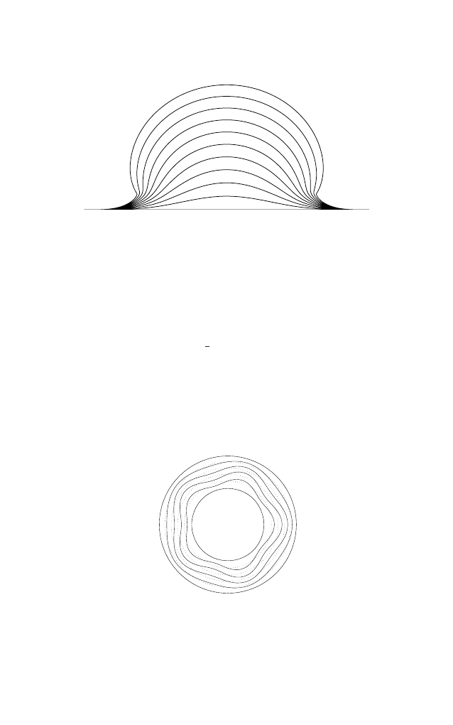
45
The geometry and curvature of shape spaces
Figure 1. A geodesic in the space of plane curves in the L
2
metric. The path
starts at the x-axis and moves in the direction of small ‘blip’. As the blip enlarges
it creates sharper and sharper corners where the curvature goes to infinity so that
the geodesic cannot be prolonged.
the wedge a
∧ b of its two tangent vector arguments. We will write
R
(a, b, a, b) as R(a ∧ b). So what could be more natural than:
R
S
(a ∧ b) =
1
2
C
(ab
− ba
)
2
ds
≥ 0
where a and b define two tangent vectors in T
[C]
S. The formula shows
that higher frequencies produce more and more positive curvature. In
fact, what happens is that path C
t
in
S can be shortened by adding high
frequency ‘wiggles’ to the intermediate curves. This is illustrated in Fig-
ure 2 below.
Figure 2. The set of all circles with fixed center is a geodesic in the L
2
metric
if the radius varies as t
2
/3
. However conjugate points are dense on it: Here
is a deformation of this geodesic which has a conjugate point when the radius
increases by the factor 1.8957.... Beyond that point, it shortens the length of the
geodesic.

46
David Mumford
To summarize: the geodesic equation is a non-linear hyperbolic PDE
with well posed initial value problem; the curvature is non-negative, go-
ing strongly to infinity at high frequency and with conjugate points dense;
and the global metric is identically zero because the infimum of path
lengths is zero. This behavior is typical of L
2
metrics.
2.
Positive curvature which is, however, tamer is produced in another
elegant situation. This example is due to the work of Laurent Younes [5,
6]. Here we regard the plane as the complex plane. The remarkable idea
is to consider the complex square root of the derivative of the curve, i.e. if
t
→ f (t) ∈ C, t ∈ R/2πR is the curve, define g(x) + ih(x) =
√
f
(t).
If C is an embedded curve (or more generally any immersed plane curve
with odd index), then g
(x + 2π) ≡ −g(x), h(x + 2π) ≡ −h(x). The
closedness of the curve is expressed by the formula
2
π
0
f
(t)dt = 0
which means that in L
2
([0, 2π]) g and h are orthogonal functions of the
same length. We can reverse this process and, starting from such a pair
g
, h, define a parameterized curve, up to translation, by:
x
−→ f (x) =
x
0
(g(x) + i.h(x))
2
d x
.
The upshot of this ansatz is this: Let
H be the Hilbert space of functions
g such that g
(x + 2π) ≡ −g(x) with norm ||g||
2
=
2
π
0
g
(x)
2
d x. Let
G be the Grassmannian of 2-planes in H and let G
0
be the open subset of
2-planes such that there is no x where all functions in the 2-plane vanish.
Then using orthonormal bases of these 2-planes as g and h, we find that
G
0
is isomorphic to the space of parameterized immersed plane curves of
odd index mod translations, rotations and scaling. Not only that but the
natural metric on this Grassmannian corresponds to a very natural metric
on this space of curves. The tangent space to parameterized curves is
given by all vector fields along the curve, not merely those which are
normal, thus, in our case, by a complex valued function along C. The
Grassmannian metric turns out to equal the 1-Sobolev norm (with only
first derivatives):
||a||
2
=
1
len
(C)
C
|a
(x)|
2
ds
(x), s = arc length.
Geodesics and curvature on a Grassmannian are given by quite simple
and classical formulas so we also get formulas for these both on this
space of parameterized curves and on its submersive quotient of unpa-
rameterized immersed curves both mod translations, rotations and scal-
ings. The geodesic equation is now an integro-differential equation most
47
The geometry and curvature of shape spaces
Figure 3. Some geodesics in Younes’s metric between plane curves representing
recognizable shapes. Note how they rotate to make optimal matches, e.g. the
tail of the cat with the head of the camel.
easily written not in terms of velocity a but in terms of a ‘momentum’
which is the second derivative u
= −d
2
a
/ds
2
. Like the Grassmannian
itself, these spaces also have entirely non-negative curvature but not so
strongly positive that this prevents the Riemannian metric from defining
a nice global metric. The space has finite diameter in its global metric
and can be completed by adding certain non-immersed curves. Some ex-
amples of geodesics in this space are shown in Figures 3 and 4. This type
of space seems to be the natural infinite dimensional analog of compact
symmetric spaces of finite dimension.
Figure 4. If we allow paths to pass through some non-immersed curves, we
find many closed geodesics in this metric. This is the simplest example. The
path goes from left to right, row by row; a loop flips over in the ellipse-like
shapes at the end of the first row and the beginning of the third, hence these are
non-immersed.

48
David Mumford
3.
A third metric can be put on simple closed plane curves, here modulo
translations and scalings, but now with non-positive curvature. Interest-
ingly, only one half a derivative is added to the metric in the previous
example: it is Sobolev with 3/2 derivatives. This is the famous Weil-
Peterson metric. It is defined as follows: start with the space of vector
fields
v(θ) on the circle and put the WP-norm on it, defined in terms of
its Fourier transform by:
||v||
2
W P
=
∞
n
=2
(n
3
− n)|ˆv
n
|
2
.
Now S L
2
is a subgroup of the group of diffeomorphisms of the circle with
lie algebra consisting of the vector fields
(a+b cos(θ)+c sin(θ))
∂
∂θ
. This
is clearly the null space of the above WP norm and since – miraculously
– the WP-norm is also invariant under the adjoint action of S L
2
, this
norm extends by right translations to an invariant Riemannian metric on
the coset space S L
2
\Diff(S
1
). Now the final link: this coset space is
isomorphic to the space of simple closed plane curves mod translations
and scalings. This comes via ‘welding’: given a diffeomorphism
ϕ, attach
two unit disks to each other along their boundaries using the twist
ϕ. The
result is a simply connected compact Riemann surface, hence it must be
conformal to the sphere. The image of the welded common boundary is
our curve. For details, see [7, 9].
One of the remarkable consequences of this construction is that it de-
fines an operation of composition between plane curves. The welding
operation also defines a bijection between the group Diff
(S
1
) itself and
triples
(C, P, "t) where C is a simple closed plane curve, P a base point
inside C and
"t is a distinguished ray at the base point, all modulo trans-
lations and scalings. Thus there is a law of composition of such triples.
Some examples are shown in Figure 5.
This metric is the closest to the standard metric on
R
n
because (a) it
is invariant under the transitive action of a group, here Diff
(S
1
) and (b)
it is quite flat in high frequency dimensions because the Ricci curvatures
(which are the sum of sectional curvatures R
(a ∧ b
i
) where {b
i
} are an
orthonormal basis of a
⊥
for variable a) are known to be finite. It is also
a complete complex K¨ahler-Hilbert manifold and has unique geodesics
between any two points [7, 8]. The metric can also be defined using po-
tential theory which embeds the curve in field lines and thus endows its
interior and exterior with a rich additional structure. The geodesic equa-
tion is an integro-differential variant of Burger’s equation involving the
(periodic) Hilbert transform. Among geodesics on this space, there is a
special class of soliton-like geodesics, which Daryll Holm named ‘tei-
49
The geometry and curvature of shape spaces
Figure 5. A selection of plane curves obtained by composing two diffeomor-
phisms corresponding to (i) a boomerang-like shape with base point in the mid-
dle and (ii) a finger-like shape with base point near one end respectively. In each
panel of 15 curves, the data
"t is varied or, equivalently, a variable rotation is
added in the middle of the composition.
chons’. They are the geodesics generated by vector fields
v dual in the
WP norm to sums of delta functions, i.e.
v, u
W P
=
i
p
i
u
(θ
i
), for all u
for some p
i
, θ
i
. An example of a teichon is shown in Figure 6.
−1
−0.5
0
0.5
1
−1
−0.8
−0.6
−0.4
−0.2
0.2
0.4
0.6
0.8
1
0
1
2
3
4
5
6
7
8
Figure 6. A geodesic from the unit circle to a duck like shape using an 8-
Teichon. The figure is due to S. Kushnarev [10].

50
David Mumford
4.
The final example is much more general and deals with the full diffeo-
morphism group of
R
n
. Arnold’s curvature formula for volume preserv-
ing diffeomorphisms was significantly more complicated than anything
in the above examples. In his case, there are both positively and neg-
atively curved sections and this also seems to happen for Riemannian
manifolds constructed from any higher order Sobolev type metrics on
diffeomorphism groups. I would not be surprised if at some point under-
standing these more complex curvature formulas gives new insight into
the unsolved problems of fluid flows.
The situation that my group has studied most intensively is the metric
induced on ‘landmark space’, that is simply the space
L
n
,N
of distinct N -
tuples of points in
R
n
. Fixing a base N -tuple, we get a submersive map
from Diff
(R
n
) to L
n
,N
. We may put a Sobolev norm on vector fields X ,
||X||
2
=
R
n
X, L Xdx
1
· · · dx
n
where L is a positive definite self-adjoint operator, e.g. L
= (I − &)
s
.
This defines a metric on the group of diffeomorphisms provided that L
has enough derivatives. In fact, we want the finiteness of the metric to
force the diffeomorphisms to be C
1
. Then we get an induced Riemannian
structure on the quotient space
L
n
,N
. It has a simple form. If G is the
Green’s function associated to L,
{P
1
, · · · P
N
} ∈ L
n
,N
and
v
a
is a vector
at P
a
, then the metric is:
||{v
1
, · · · , v
N
}||
2
=
1
≤a,b≤N
(G
−1
)
ab
v
a
, v
b
, G
ab
= G(P
a
− P
b
).
Arguably this is the most natural class of metrics to put on landmark
space.
The geodesic equation on landmark space is quite elegant. To any
geodesic there is a natural set of momenta u
a
for which a geodesic is a
solution of:
du
a
dt
= −
b
∇G(P
a
− P
b
)u
a
, u
b
d P
a
dt
=
b
G
(P
a
− P
b
)u
b
.
These equations create a world governed by a weird sort of physics in
which points moving together attract and points moving in opposite di-
rections repel and occasionally one even gets planetary systems. Since
L
n
,N
is a submersive quotient of the diffeomorphism group, geodesics in
L lift to horizontal geodesics in the group. So these geodesics induce
51
The geometry and curvature of shape spaces
warpings of the ambient Euclidean space. In fact any geodesic in the
diffeomorphism group can be approximated by one of these landmark
geodesics if we take enough landmark points. Some examples are shown
in Figure 6.
Figure 7. Three geodesics on the landmark spaces
L
2
,2
, L
2
,2
, L
2
,4
respectively,
plus the induced diffeomorphism of the ambient plane. Note how points moving
in the same (resp. opposite) direction are drawn together (resp. pushed apart).
In the four point case, this causes some complex gyrations. These figures are
from the thesis of M. Micheli [11]
The sectional curvature of landmark space has four terms, similarly to
Arnold’s formula for the curvature of Lie groups [1]. The reason for
this seems to be that it reflects several different modes of interactions
of the points. There are, in particular, at least two ‘causes’ of positive
curvature. One is seen in the middle panel of Figure 4: when two points
must move in a similar direction, it saves energy for them to come close
to each other. But if the distances are in a certain range, there will be two
geodesics joining the pair at the initial position on the left and the same
pair translated to the final position on the right. One geodesic has the
points moving nearly independently and nearly parallel and the other has

52
David Mumford
them first coming close, then moving together and finally moving apart
again. This non-uniqueness causes positive curvature.
Another cause of positive curvature occurs in dimension three and
higher. Suppose two points are to be interchanged, the first moving to
the position of the second and the second to that of the first. Since the
distance is infinite if they were to move directly towards each other, they
must move around each other and there are many planes in which to do
this. We show in [12] that when only two points have momenta, these
are, in a sense, the only ways positive curvature can arise.
But negative curvature arises all the time from the turbulence caused
by landmark point motion. Take the situation where a single point P is
moving with non-zero momentum but that there are many other landmark
points around it with zero momentum. These extra points are dragged
along, compressed together in front of P. If P moves from A to B, we
wind up with a configuration C
(B) of the whole set of landmarks. Take
B
1
= B
2
. Then what will the geodesic from C
(B
1
) to C(B
2
) look like?
You can’t just put momentum on P because you need to move the points
bunched up near B
1
back apart and create a new bunch near B
2
. The only
way to do this is unwind the mess you made in one geodesic and recreate
the new mess in the second. This is negative curvature: to connect the
endpoints of two trips, it is better to go nearly back home. For details,
see [12].
Anyway, the somewhat daunting formula for sectional curvature is this.
Let
v
1
= {v
a
1
} and v
2
= {v
a
2
} be two tangent vectors to T L at some point
{P
a
}. Let v
i
be extended to a vector field on
R
n
by its horizontal lift to
the diffeomorphism group. Let
v
1
and
v
2
be the co-vectors dual to the
v’s. Then the numerator of sectional curvature is given by:
R
(v
1
∧ v
2
) = R
1
+ R
2
+ R
3
+ R
4
R
1
=
1
2
a
=b
(v
2
)
a
⊗ δ
ab
v
1
− (v
1
)
a
⊗ δ
ab
v
2
· H
ab
·
(v
2
)
b
⊗ δ
ab
v
1
− (v
1
)
b
⊗ δ
ab
v
2
,
R
2
=
D
11
, F
22
−
D
12
+ D
21
, F
12
)
+
D
22
, F
11
,
R
3
=
F
12
2
T
∗
L
−
F
11
, F
22
T
∗
L
,
R
4
= −
3
4
D
12
− D
21
)
2
T
L
,
where
δ
ab
v = v
a
− v
b
, and C
ab
(v) =
δ
ab
v, ∇G(P
a
− P
b
)
for any
v
and D
a
i j
=
b
=a
C
ab
(v
i
)(v
j
)
b
∈ T L,
and
(F
i j
)
a
=
1
2
D
a
v
i
· (v
j
)
a
+ D
a
v
j
· (v
i
)
a
∈ T
∗
L, (D
a
=deriv. at P
a
)
and H
ab
= I ⊗ D
2
G
(P
a
− P
b
).

53
The geometry and curvature of shape spaces
The term R
4
above is the main cause of the turbulence related negative
curvature: it is the only term which involves points with no momentum
of their own.
It is natural to generalize this formula to get more insight into it. A
paper is under preparation analyzing the spaces of submanifolds of any
type in any fixed ambient finite dimensional manifold M with respect to a
very general Sobolev-type metric on the group of diffeomorphisms of M.
References
[1] V. A
RNOLD
, Sur la g´eom´etrie diff`erentielle des groupes de Lie de
dimension infinie et ses applications l’hydrodynamique des fluides
parfaits, Annales de l’institut Fourier 16 (1966), 319–36.
[2] P. M
ICHOR
and D. M
UMFORD
, Riemannian Geometries on Spaces
of Plane Curves, J. of the Europ Math. Society 8 (2006), 1–48.
[3] P. M
ICHOR
and D. M
UMFORD
, Vanishing geodesic distance on
spaces of submanifolds and diffeomorphisms, Documenta Mathemat-
ica, 10, 2005.
[4] P. M
ICHOR
and D. M
UMFORD
, An overview of the Riemannian met-
rics on spaces of curves using the Hamiltonian Approach, Applied
and Computational Harmonic Analysis 23 (2007), 74–113.
[5] L. Y
OUNES
, Computable elastic distances between shapes, SIAM J.
Appl. Math. 58 (1998), 565-586.
[6] P. M
ICHOR
, D. M
UMFORD
, J. S
HAH
and L. Y
OUNES
, A metric on
shape space with explicit geodesics, Rendiconti Lincei – Matematica
e Applicazioni 19 (2009), 25–57.
[7] T. T
AKHTAJAN
and L.-P. T
EO
, “Weil-Petersson Metric on Universal
Teicm¨uller Space”, Memoirs of the AMS, Vol. 86, 2008.
[8] F. G
AY
-B
ALMAZ
, “Infinite Dimensional Flows and the Universal
Teichm¨uller Space”, PhD thesis, ´
Ecole Polytechnique de Lausanne,
2009.
[9] D. M
UMFORD
and E. S
HARON
, 2D-Shape Analysis using Con-
formal Mapping (with Eitan Sharon), Int. J. of Comp. Vision 70
(2006),55–75.
[10] S. K
USHNAREV
, Teichon: Soliton-like Geodesics on Universal Te-
ichm¨uller Space, J. Exp. Math. 18 (2009), 325-336.
[11] M. M
ICHELI
, “The Differential Geometry of Landmark Shape
Manifolds”, PhD thesis, Div. of Appl. Math., Brown Univ., 2008.
[12] M. M
ICHELI
, P. M
ICHOR
and D. M
UMFORD
, Sectional curvature
in terms of the Cometric, with applications to the Riemannian mani-
folds of Landmarks, submitted.

COLLOQUIA
The volumes of this series reflect lectures held at the “Colloquio De
Giorgi” which regularly takes place at the Scuola Normale Superiore in
Pisa. The Colloquia address a general mathematical audience, particu-
larly attracting advanced undergraduate and graduate students.
Published volumes
1. Colloquium De Giorgi 2006.
ISBN 978-88-7642-212-6
2. Colloquium De Giorgi 2007 and 2008.
ISBN 978-88-7642-344-4
3. Colloquium De Giorgi 2009.
ISBN 978-88-7642-388-8, e-ISBN 978-88-7642-387-1
Document Outline
- Cover
- Title Page
- Copyright Page
- Table of Contents
- Preface
- Isomorphisms of the Figà-Talamanca–Herz algebras Ap(G) for connected Lie groups G
- Classical analysis and nilpotent Lie groups
- Leibniz’ conjecture, periods & motives
- The geometry and curvature of shape spaces
- Back matter
Wyszukiwarka
Podobne podstrony:
TESTcałościowy z chirurgii 2008-2009, ratownicto 2012 2013, ratownictwo medyczne, Testy
sesja 28.11.2009, Rok 2012, Channeling, Kasjopeanie, Transkrypty sesji channelingowych
TEST rany dla ucznia 2008-2009, ratownicto 2012 2013, ratownictwo medyczne, Testy
TEST- końcowy z chirurgii dla ucznia 2008-2009, ratownicto 2012 2013, ratownictwo medyczne, Testy
sesja z 15.08.2009, Rok 2012, Channeling, Kasjopeanie, Transkrypty sesji channelingowych
ustawa z dn 02 04 2009 Dz U 2012 161, Prawo, Rok 3, Prawo Międzynarodowe Publiczne
1001 QUESTÕES DE CONCURSO PORTUGUÊS FCC 2012
wikileaks de raid 2009
Improve Your Punctuation and Grammar Marion Field 3rd ed How To Books 2009
The New Age of Russia Occult and Esoteric Dimensions ed by B Menzel & M Hagemeister & BG Rosenthal
Kobyłecka, Ewa Orientación temporal del relato de ficción (2009)
Monarch The New Phoenix Program ed by Marshall G Thomas (2009)
5 7) 1001 QUESTÕES DE CONCURSO INFORMATICA FCC 2012
7 7) 1001 QUESTÕES DE CONCURSO RLM FCC 2012
Kushner A G Three lectures on contact geometry of Monge Ampere equations (Univ de Los Andes, Bogota,
Meziani A On first and second order planar elliptic equations with degeneracies (MEMO1019, AMS, 2012
Iwaniec T , Onninen J n harmonic mappings between annuli the art of integrating free Lagrangians (M
Lax P D , Zalcman L Complex proofs of real theorems (ULECT058, AMS, 2012)(ISBN 9780821875599)(O)(106
więcej podobnych podstron