Fitting Models

359

1040-9238/00/$.50
© 2000 by CRC Press LLC

Critical Reviews in Biochemistry and Molecular Biology, 35(5):359–391 (2000)

Beyond Eyeballing: Fitting Models to
Experimental Data

Arthur Christopoulos and Michael J. Lew

Table of Contents

Introduction ............................................................................................. 361
A.

“Eyeballing” ..................................................................................... 361

Models .............................................................................................. 361

II.

Empirical or Mechanistic? ..................................................................... 361

III.

Types of Fitting ....................................................................................... 363
A.

Correlation ........................................................................................ 363
1.

The Difference Between Correlation and Linear
Regression ............................................................................... 363

The Meaning of r

................................................................... 363

Assumptions of Correlation Analysis ..................................... 364

Misuses of Correlation Analysis ............................................. 364

Regression ........................................................................................ 365
1.

Linear Regression .................................................................... 365

Ordinary Linear Regression .................................................... 365

Multiple Linear Regression ..................................................... 365

Nonlinear Regression .............................................................. 367

Assumptions of Standard Regression Analyses...................... 367

IV.

How It Works .......................................................................................... 368
A.

Minimizing an Error Function (Merit Function) ............................. 368

Least Squares .................................................................................... 368

Nonleast Squares .............................................................................. 371

Weighting.......................................................................................... 371

Regression Algorithms ..................................................................... 372

When to Do It (Application of Curve Fitting Procedures) ................ 374
A.

Calibration Curves (Standard Curves) ............................................. 374

Parameterization of Data (Distillation) ............................................ 374

Critical Reviews in Biochemistry and Molecular Biology Downloaded from informahealthcare.com by 83.26.195.157 on 11/28/10

For personal use only.

360

VI.

How to Do It ............................................................................................ 374
A.

Choosing the Right Model ............................................................... 374
1.

Number of Parameters ............................................................ 374

Shape ....................................................................................... 375

Correlation of Parameters ....................................................... 376

Distribution of Parameters ...................................................... 376

Assessing the Quality of the Fit ...................................................... 377
1.

Inspection................................................................................. 377

Root Mean Square ................................................................... 377

(Coefficient of Determination)........................................... 378

Analysis of Residuals .............................................................. 379

The Runs Test .......................................................................... 379

Optimizing the Fit ............................................................................ 380
1.

Data Transformations .............................................................. 380

Initial Estimates ....................................................................... 381

Reliability of Parameter Estimates .................................................. 382
1.

Number of Datapoints ............................................................. 382

Parameter Variance Estimates from Repeated
Experiments ............................................................................. 383

Parameter Variance Estimates from Asymptotic
Standard Errors ........................................................................ 384

Monte Carlo Methods ............................................................. 385

The Bootstrap .......................................................................... 386

Grid Search Methods .............................................................. 387

Evaluation of Joint Confidence Intervals ............................... 387

Hypothesis Testing ........................................................................... 387
1.

Assessing Changes in a Model Fit between
Experimental Treatments ......................................................... 387

Choosing Between Models ..................................................... 388

VII. Fitting Versus Smoothing ....................................................................... 388

VIII. Conclusion ................................................................................................ 389

IX.

Software ................................................................................................. 389

References

................................................................................................. 390

Critical Reviews in Biochemistry and Molecular Biology Downloaded from informahealthcare.com by 83.26.195.157 on 11/28/10

For personal use only.

361

I. INTRODUCTION

A. “Eyeballing”

The oldest and most commonly used

tool for examining the relationship between
experimental variables is the graphical dis-
play. People are very good at recognizing
patterns, and can intuitively detect various
modes of behavior far more easily from a
graph than from a table of numbers. The
process of “eyeballing the data” thus repre-
sents the experimenter’s first attempt at
understanding their results and, in the past,
has even formed the basis of formal quanti-
tative conclusions. Eyeballing can some-
times be assisted by judicious application of
a ruler, and often the utility of the ruler has
been enhanced by linearizing data transfor-
mations. Nowadays it is more common to
use a computer-based curve-fitting routine
to obtain an “unbiased” analysis. In some
common circumstances there is no impor-
tant difference in the conclusions that would
be obtained by the eye and by the computer,
but there are important advantages of the
more modern methods in many other cir-
cumstances. This chapter will discuss some
of those methods, their advantages, and how
to choose between them.

B. Models

The modern methods of data analysis

frequently involve the fitting of mathemati-
cal models to the data. There are many rea-
sons why a scientist might choose to model
and many different conceptual types of
models. Modeling experiments can be en-
tirely constructed within a computer and
used to test “what if” types of questions
regarding the underlying mathematical as-

pects of the system of interest. In one sense,
scientists are constructing and dealing with
models all the time inasmuch as they form
“worldview” models; experiments are de-
signed and conducted and then used in an
intuitive fashion to build a mental picture of
what the data may be revealing about the
experimental system (see Kenakin, this vol-
ume). The experimental results are then fre-
quently analyzed by applying either empiri-
cal or mechanistic mathematical models to
the data. It is these models that are the sub-
ject of this article.

II. EMPIRICAL OR MECHANISTIC?

Empirical models are simple descrip-

tors of a phenomenon that serve to approxi-
mate the general shape of the relationship
being investigated without any theoretical
meaning being attached to the actual pa-
rameters of the model. In contrast, mecha-
nistic models are primarily concerned with
the quantitative properties of the relation-
ship between the model parameters and its
variables, that is, the processes that govern
(or are thought to govern) the phenomenon
of interest. Common examples of mecha-
nistic models are those related to mass ac-
tion that are applied to binding data to ob-
tain estimates of chemical dissociation
constants whereas nonmechanistic, empiri-
cal models might be any model applied to
drug concentration–response curves in or-
der to obtain estimates of drug potency. In
general, mechanistic models are often the
most useful, as they consist of a quantitative
formulation of a hypothesis.

However, the

consequences of using an inappropriate
mechanistic model are worse than for em-
pirical models because the parameters in
mechanistic models provide information
about the quantities and properties of real
system components. Thus, the appropriate-

Critical Reviews in Biochemistry and Molecular Biology Downloaded from informahealthcare.com by 83.26.195.157 on 11/28/10

For personal use only.

362

ness of mechanistic models needs close scru-
tiny.

The designation of a mathematical model

as either empirical or mechanistic is based
predominantly on the purpose behind fitting
the model to experimental data. As such,
the same model can be both empirical and
mechanistic depending on its context of use.
As an example, consider the following form
of the Hill equation:

(1)

This equation is often used to analyze

concentration–occupancy curves for the in-
teraction of radioligands with receptors or
concentration–response curves for the func-
tional interaction of agonist drugs with re-
ceptors in cells or tissues. The Hill equation
describes the observed experimental curve
in terms of the concentration of drug (A), a
maximal asymptote (

), a midpoint loca-

tion (K), and a midpoint slope (S). In prac-
tice, these types of curves are most conve-
niently visualized on a semi-logarithmic
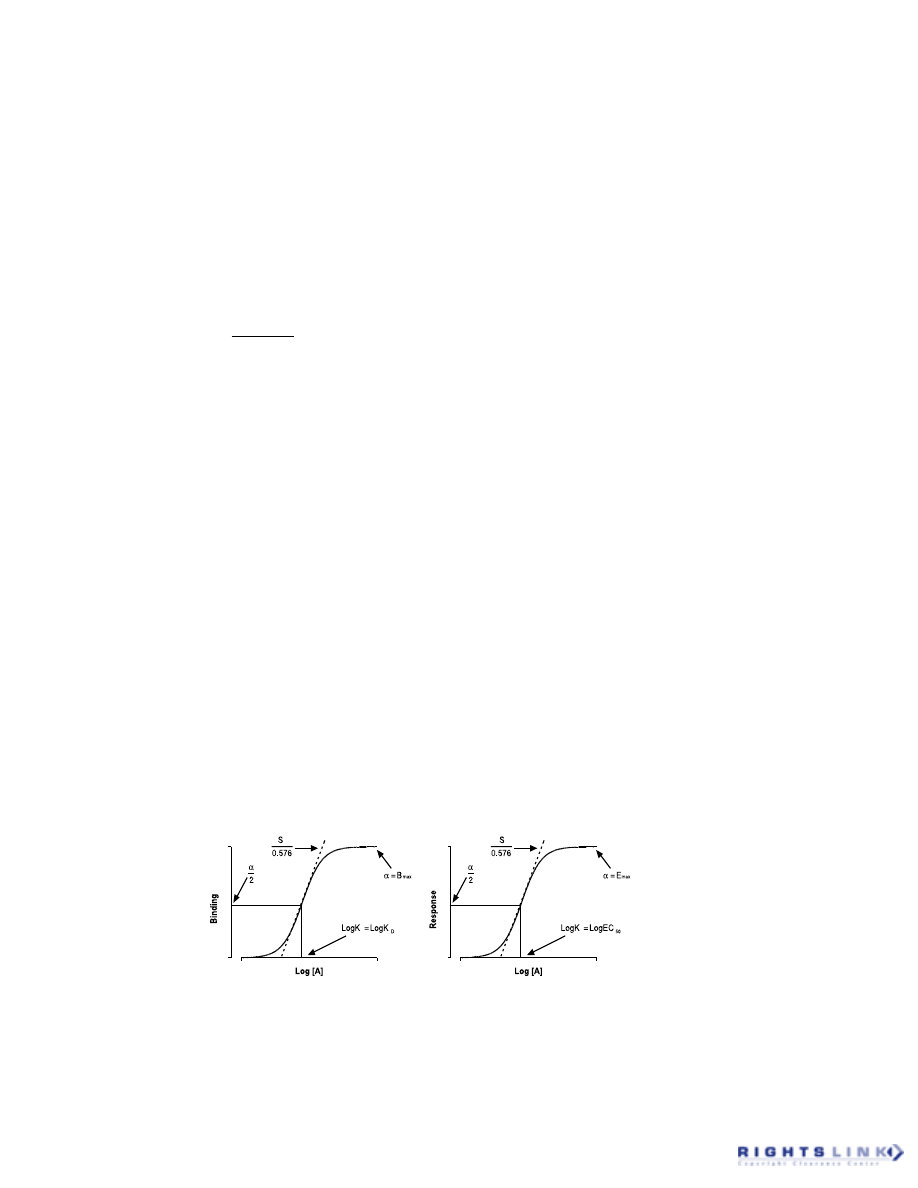
scale, as shown in Figure 1.

When Hill first derived this equation,

2,3

he based it on a mechanistic model for the
binding of oxygen to the enzyme, hemoglo-
bin. In that context, the parameters that Hill
was interested in, K and S, were meant to
reveal specific biological properties about
the interaction he was studying; K was a
measure of the affinity of oxygen for the

enzyme and S was the number of molecules
of oxygen bound per enzyme. Subsequent
experiments over the years have revealed
that this model was inadequate in account-
ing for the true underlying molecular mecha-
nism of oxygen-hemoglobin binding, but
the equation remains popular both as a
mechanistic model when its validity is ac-
cepted, and as an empirical model where its
shape approximates that of experimental
data. For instance, if the experimental curve
is a result of the direct binding of a
radioligand to a receptor, then application
of Equation (1) to the dataset can be used to
detect whether the interaction conforms to
the simplest case of one-site mass-action
binding and, if S = 1, the parameters K and

can be used as quantitative estimates of

the ligand-receptor dissociation constant
(K

) and total density of receptors (B

max

respectively. This is an example where the
Hill equation is a mechanistic equation,
because the resulting parameters provide
actual information about the underlying
properties of the interaction. In contrast,
concentration–response curves represent the
final element in a series of sequential bio-
chemical cascades that yield the observed
response subsequent to the initial mass-ac-
tion binding of a drug to its receptor. Thus,
although the curve often retains a sigmoidal
shape that is similar to the binding curve,
the Hill equation is no longer valid as a
mechanistic equation. Hence, the Hill equa-

[ ]

FIGURE 1. Concentration–binding (left) and concentration–response (right) curves showing the
parameters of the Hill equation (

, K, and S) as mechanistic (left) or empirical (right) model

descriptors.

Critical Reviews in Biochemistry and Molecular Biology Downloaded from informahealthcare.com by 83.26.195.157 on 11/28/10

For personal use only.

363

tion is useful in providing a good fit to
sigmoidal concentration–response curves,
but the resulting parameters are considered
empirical estimates of maximal response,
midpoint slope, and midpoint location, and
no mechanistic interpretation should be
made.

III. TYPES OF FITTING

The variables whose relationships that

can be plotted on Cartesian axes do not
necessarily have the same properties. Often
one variable is controlled by the experi-
menter and the other variable is a measure-
ment. Thus one variable has substantially
more uncertainty or variability than the other,
and traditionally that variable would be plot-
ted on the vertical axis. In that circumstance
the Y variable can be called the “depen-
dent” variable because of its dependence on
the underlying relationship and on the other
variable, which is called “independent” to
denote its higher reliability. It is important
to note that not all datasets have a clearly
independent variable. Historically, the sta-
tistical determination of the relationship
between two or more dependent variables
has been referred to as a correlation analy-
sis, whereas the determination of the rela-
tionship between dependent and indepen-
dent variables has come to be known as a
regression analysis. Both types of analyses,
however, can share a number of common
features, and some are discussed below.

A. Correlation

Correlation is not strictly a regression

procedure, but in practice it is often confused
with linear regression. Correlation quantifies
the degree by which two variables vary to-

gether. It is meaningful only when both vari-
ables are outcomes of measurement such that
there is no independent variable.

1. The Difference between
Correlation and Linear
Regression

Correlation quantifies how well two

dependent variables vary together; linear
regression finds the line that best predicts a
dependent variable given one or more inde-
pendent variables, that is, the “line of best-
fit.”

Correlation calculations do not find a

best-fit straight line.

2. The Meaning of r

The direction and magnitude of the cor-

relation between two variables can be quan-
tified by the correlation coefficient, r, whose
values can range from –1 for a perfect nega-
tive correlation to 1 for a perfect positive
correlation. A value of 0, of course, indi-
cates a lack of correlation. In interpreting
the meaning of r, a difficulty can arise with
values that are somewhere between 0 and –
1 or 0 and 1. Either the variables do influ-
ence each other to some extent, or they are
under the influence of an additional factor
or variable that was not accounted for in the
experiment and analysis. A better “feel” for
the covariation between two variables may
be derived by squaring the value of the
correlation coefficient to yield the coeffi-
cient of determination, or r

value. This

number may be defined as the fraction of
the variance in the two variables that is
shared, or the fraction of the variance in one
variable that is explained by the other (pro-
vided the following assumptions are valid).
The value of r

, of course, will always be

between 0 and 1.

Critical Reviews in Biochemistry and Molecular Biology Downloaded from informahealthcare.com by 83.26.195.157 on 11/28/10

For personal use only.

364

3. Assumptions of Correlation
Analysis

The subjects are randomly selected
from a larger population. This is often
not true in biomedical research, where
randomization is more common than
sampling, but may be sufficient to as-
sume that the subjects are at least rep-
resentative of a larger population.

The samples are paired, i.e., each experi-
mental unit has both X and Y values.

The observations are independent of
each other. Sampling one member of
the population should not affect the
probability of sampling another mem-
ber (e.g., making measurements in the
same subject twice and treating them
as separate datapoints; making mea-
surements in siblings).

The measurements are independent. If
X is somehow involved or connected
to the determination of Y, or vice versa,
then correlation is not valid. This as-
sumption is very important because
artifactual correlations can result from
its violation. A common cause of such
a problem is where the Y value is ex-
pressed as either a change from the X
value, or as a fraction of the corre-
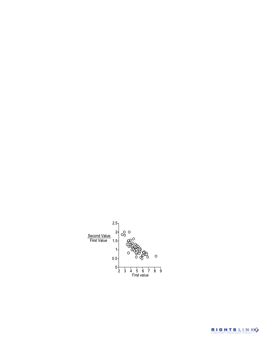
sponding X value (Figure 2).

The X values were measurements, not
controlled (e.g., concentration, etc.).
The confidence interval for r

is other-

wise meaningless, and we must then
use linear regression.

The X and Y values follow a Gaussian
distribution.

The covariation is linear.

4. Misuses of Correlation
Analysis

Often, biomedical investigators are in-

terested in comparing one method for mea-
suring a biological response with another.
This usually involves graphing the results as
an X, Y plot, but what to do next? It is quite
common to see a correlation analysis applied
to the two methods of measurement and the
correlation coefficient, r, and the resulting P
value utilized in hypothesis testing. How-
ever, Ludbrook

has outlined some serious

criticisms of this approach, the major one
being that although correlation analysis will
identify the strength of the linear association
between X and Y, as it is intended to do, it
will give no indication of any bias between
the two methods of measurement. When the
purpose of the exercise is to identify and
quantify fixed and proportional biases be-

FIGURE 2. An apparent correlation between two sets of unrelated random numbers (pseudo-
random numbers generated with mean = 5 and standard deviation = 1) comes about where the Y
value is expressed as a function of the X value (here each Y value is expressed as a fraction of
the corresponding X value).

Critical Reviews in Biochemistry and Molecular Biology Downloaded from informahealthcare.com by 83.26.195.157 on 11/28/10

For personal use only.

365

tween two methods of measurement, then
correlation analysis is inappropriate, and a
technique such as ordinary or weighted least
products regression

should be used.

B. Regression

The actual term “regression” is derived

from the latin word “regredi,” and means
“to go back to” or “to retreat.” Thus, the
term has come to be associated with those
instances where one “retreats” or “resorts”
to approximating a response variable with
an estimated variable based on a functional
relationship between the estimated variable
and one or more input variables. In regres-
sion analysis, the input (independent) vari-
ables can also be referred to as “regressor”
or “predictor” variables.

1. Linear Regression

The most straightforward methods for

fitting a model to experimental data are those
of linear regression. Linear regression in-
volves specification of a linear relationship
between the dependent variable(s) and cer-
tain properties of the system under investi-
gation. Surprisingly though, linear regres-
sion deals with some curves (i.e., nonstraight
lines) as well as straight lines, with regres-
sion of straight lines being in the category
of “ordinary linear regression” and curves
in the category of “multiple linear regres-
sions” or “polynomial regressions.”

2. Ordinary Linear Regression

The simplest general model for a straight

line includes a parameter that allows for

inexact fits: an “error parameter” which we
will denote as

. Thus we have the formula:

Y =

X +

(2)

The parameter,

, is a constant, often

called the “intercept” while b is referred to
as a regression coefficient that corresponds
to the “slope” of the line. The additional
parameter,

, accounts for the type of error

that is due to random variation caused by
experimental imprecision, or simple fluc-
tuations in the state of the system from one
time point to another. This error term is
sometimes referred to as the stochastic com-
ponent of the model, to differentiate it from
the other, deterministic, component of the
model (Figure 3).

When data are fitted to

the actual straight-line model, the error term
denoted by

is usually not included in the

fitting procedure so that the output of the
regression forms a perfect straight line based
solely on the deterministic component of
the model. Nevertheless, the regression pro-
cedure assumes that the scatter of the
datapoints about the best-fit straight line
reflects the effects of the error term, and it
is also implicitly assumed that

follows a

Gaussian distribution with a mean of 0. This
assumption is often violated, however, and
the implications are discussed elsewhere in
this article. For now, however, we will as-
sume that the error is Gaussian; Figure 4
illustrates the output of the linear model
with the inclusion of the error term. Note
that the Y values of the resulting “line” are
randomly distributed above and below the
ideal (dashed) population line defined by
the deterministic component of the model.

3. Multiple Linear Regression

The straight line equation [Equation (2)]

is the simplest form of the linear regression

Critical Reviews in Biochemistry and Molecular Biology Downloaded from informahealthcare.com by 83.26.195.157 on 11/28/10

For personal use only.

366

model, because it only includes one inde-
pendent variable. When the relationship of
interest can be described in terms of more
than one independent variable, the regres-
sion is then defined as “multiple linear re-
gression.” The general form of the linear
regression model may thus be written as:

Y =

+ … +

(3)

where Y is the dependent variable, and X1,
X2 … Xi are the (multiple) independent
variables. The output of this model can de-
viate from a straight line, and one may thus
question the meaning of the word “linear”
in “linear regression.” Linear regression
implies a linear relationship between the
dependent variable and the parameters, not
the independent variables of the model. Thus
Equation (3) is a linear model because the
parameters

…

have the (implied)

exponent of unity. Multiple linear regres-
sion models also encompass polynomial
functions:

Y =

X +

+ … +

(4)

The equation for a straight line [Equa-

tion (2)] is a first-order polynomial. The
quadratic equation, Y =

X +

, is

a second-order polynomial whereas the cu-
bic equation, Y =

X +

a third-order polynomial. Each of these
higher order polynomial equations defines
curves, not straight lines. Mathematically, a
linear model can be identified by taking the
first derivative of its deterministic compo-
nent with respect to the parameters of the

model. The resulting derivatives should not
include any of the parameters; otherwise,
the model is said to be “nonlinear.” Con-
sider the following second-order polyno-
mial model:

Y =

X +

(5)

Taking first derivatives with respect to

each of the parameters yields:

(6)

(7)

(8)

The model is linear because the first

derivatives do not include the parameters.
As a consequence, taking the second (or
higher) order derivative of a linear func-
tion with respect to its parameters will
always yield a value of zero.

Thus, if the

independent variables and all but one pa-
rameter are held constant, the relationship
between the dependent variable and the
remaining parameter will always be lin-
ear.

It is important to note that linear re-

gression does not actually test whether
the data sampled from the population fol-
low a linear relationship. It assumes lin-
earity and attempts to find the best-fit
straight line relationship based on the data
sample.

FIGURE 3. The simple linear population model equation indicating the deterministic component of
the model that is precisely determined by the parameters

and

, and the stochastic component

of the model,

, that represents the contribution of random error to each determined value of Y.

∂

∂α

∂

∂β

∂

∂β

Critical Reviews in Biochemistry and Molecular Biology Downloaded from informahealthcare.com by 83.26.195.157 on 11/28/10

For personal use only.

367

4. Nonlinear Regression

Because there are so many types of

nonlinear relationships, a general model that
encompasses all their behaviors cannot be
defined in the sense used above for linear
models, so we will define an explicit non-
linear function for illustrative purposes. In
this case, we will use the Hill equation [Equa-
tion (1); Figure 1] which contains one inde-
pendent variable [A], and 3 parameters,

K, and S. Differentiating Y with respect to
each model parameter yields the following:

(9)

(10)

(11)

All derivatives involve at least two of

the parameters, so the model is nonlinear.
However, it can be seen that the partial
derivative in Equation (9) does not contain
the parameter,

. A linear regression of Y

on [A]

/(K

+ [A]

) will thus allow the es-

timation of

. Because this last (linear) re-

gression is conditional on knowing the val-

ues of K and S,

is referred to as a “condi-

tionally linear” parameter. Nonlinear mod-
els that contain conditionally linear param-
eters have some advantages when it comes
to actual curve fitting.

5. Assumptions of Standard
Regression Analyses

4,7

The subjects are randomly selected
from a larger population. The same
caveats apply here as with correlation
analyses.

The observations are independent.

X and Y are not interchangeable. Re-
gression models used in the vast ma-
jority of cases attempt to predict the
dependent variable, Y, from the in-
dependent variable, X and assume
that the error in X is negligible. In
special cases where this is not the
case, extensions of the standard re-
gression techniques have been de-
veloped to account for nonnegligible
error in X.

The relationship between X and Y is
of the correct form, i.e., the expecta-
tion function (linear or nonlinear
model) is appropriate to the data being
fitted.

The variability of values around the
line is Gaussian.

∂

∂α

[ ]

∂
∂

S K A

K A

= −

( [ ])

([ ]

)

∂
∂

S K A

K A

= −

( [ ])

([ ]

)

FIGURE 4. A linear model that incorporates a stochastic (random error) component. The dashed
line is the deterministic component, whereas the points represent the effect of random error
[denoted by the symbol

in Equation (2)].

Critical Reviews in Biochemistry and Molecular Biology Downloaded from informahealthcare.com by 83.26.195.157 on 11/28/10

For personal use only.

368

The values of Y have constant vari-
ance. Assumptions 5 and 6 are often
violated (most particularly when the
data has variance where the standard
deviation increases with the mean) and
have to be specifically accounted for
in modifications of the standard re-
gression procedures.

There are enough datapoints to pro-
vide a good sampling of the random
error associated with the experimental
observations. In general, the minimum
number of independent points can be
no less than the number of parameters
being estimated, and should ideally be
significantly higher.

IV. HOW IT WORKS

A. Minimizing an Error Function
(Merit Function)

The goal of both linear and nonlinear

regression procedures is to derive the “best
fit” of a particular model to a set of experi-
mental observations. To obtain the best-fit
curve we have to find parameter values that
minimize the difference between the ob-
served experimental observations and the
chosen model. This difference is assumed
to be due to the error in the experimental
determination of the datapoints, and thus it
is common to see the entire model-fitting
process described in terms of “minimiza-
tion of an error function” or minimization
of a “merit function.”

The most common representation

(“norm”) of the merit function for regres-
sion models is based on the chi-square dis-
tribution. This distribution and its associ-
ated statistic,

, have long been used in the

statistical arena to assess “goodness-of-fit”
with respect to identity between observed

and expected frequencies of measures. Be-
cause regression analyses also involve the
determination of the best model estimates
of the dependent variables based on the
experimentally observed dependent vari-
ables, it is quite common to see the function
used to determine the best-fit of the model
parameters to the experimental data referred
to as the “

function,” and the procedure

referred to as “chi-square fitting.”

B. Least Squares

The most widely used method of pa-

rameter estimation from curve fitting is the
method of least squares. To explain the prin-
ciple behind least squares methods, we will
use an example, in this case the simple lin-
ear model. Theoretically, finding the slope,

, and intercept,

, parameters for a perfect

straight line is easy: any two X,Y pairs of
points can be utilized in the familiar “rise-
over-run” formulation to obtain the slope
parameter, which can then be inserted into
the equation for the straight line to derive
the intercept parameter. In reality, however,
experimental observations that follow lin-
ear relationships almost never fall exactly
on a straight line due to random error. The
task of finding the parameters describing
the line is thus no longer simple; in fact, it
is unlikely that values for

and

defined

by any pair of experimental points will de-
scribe the best line through all the points.
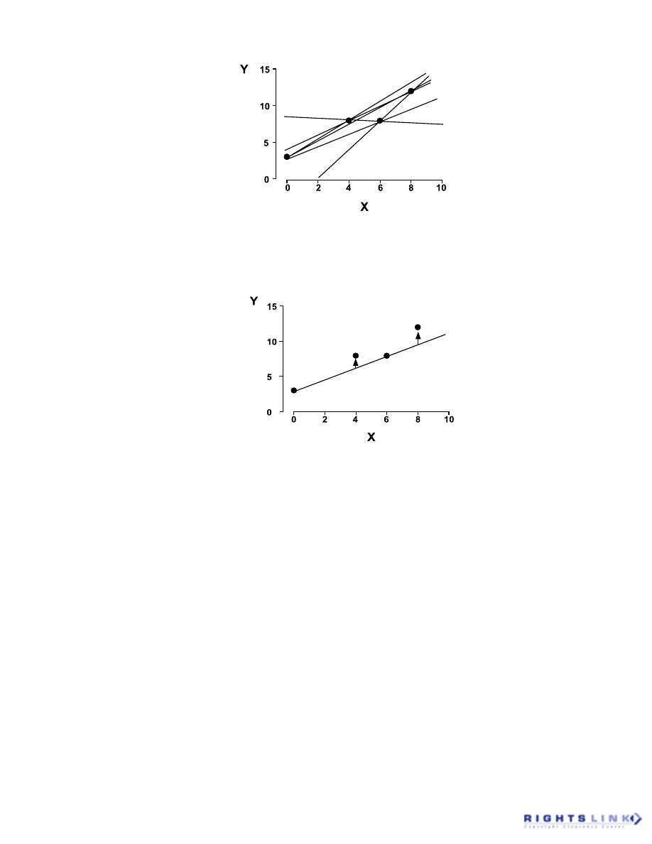
This is illustrated in Figure 5; although the
dataset appears to follow a linear relation-
ship, it can be seen that different straight
lines, each characterized by different slopes
and intercepts, are derived depending on
which two X,Y pairs are used.

What is needed, therefore, is a “com-

promise” method for obtaining an objective
best-fit. We begin with our population model
[Equation (2)]:

Critical Reviews in Biochemistry and Molecular Biology Downloaded from informahealthcare.com by 83.26.195.157 on 11/28/10

For personal use only.

369

Y =

X +

and derive an equation that is of the same
form:

Y =

ˆ +

ˆ X

(12)

where ˆ

Y is the predicted response and

and

ˆ are the estimates of the population

intercept and slope parameters, respectively.
The difference between the response vari-
able, Y, and its predictor, ˆ

Y, is called the

“residual” and its magnitude is therefore a
measure of how well ˆ

Y predicts Y. The

closer the residual is to a value of zero for

each experimental point, the closer the pre-
dicted line will be to that point. However,
because of the error in the data (the

term

in the population model), no prediction equa-
tion will fit all the datapoints exactly and,
hence, no equation can make the residuals
all equal zero. In the example above, each
straight line will yield a residual of zero for
two points, but a nonzero residual for the
other two points; Figure 6 illustrates this for
one of the lines.

A best-fit compromise is found by mini-

mizing the sum of the squares of the residu-
als, hence the name “least squares.” Math-
ematically, the appropriate merit function
can be written as:

FIGURE 5. All possible straight lines that can be drawn through a four-point dataset when only two
points are used to define each line.

FIGURE 6. A combination of zero and nonzero residuals. The dataset is the same as in Figure 5,
with only one of the lines now drawn through the points. The vertical distance of each point from
the line (indicated by the arrows) is defined as the “residual.”

Critical Reviews in Biochemistry and Molecular Biology Downloaded from informahealthcare.com by 83.26.195.157 on 11/28/10

For personal use only.

370

(13)

where

is the weighted sum of the squares

of the residuals (ri) and is a function of the
parameters (the vector,

), and the N

datapoint, X

. The term, w

, is the statisti-

cal weight (see below) of a particular
datapoint, and when used, most often re-
lates to the standard error of that point. For
standard (unweighted) least squares proce-
dures such as the current example, wi equals
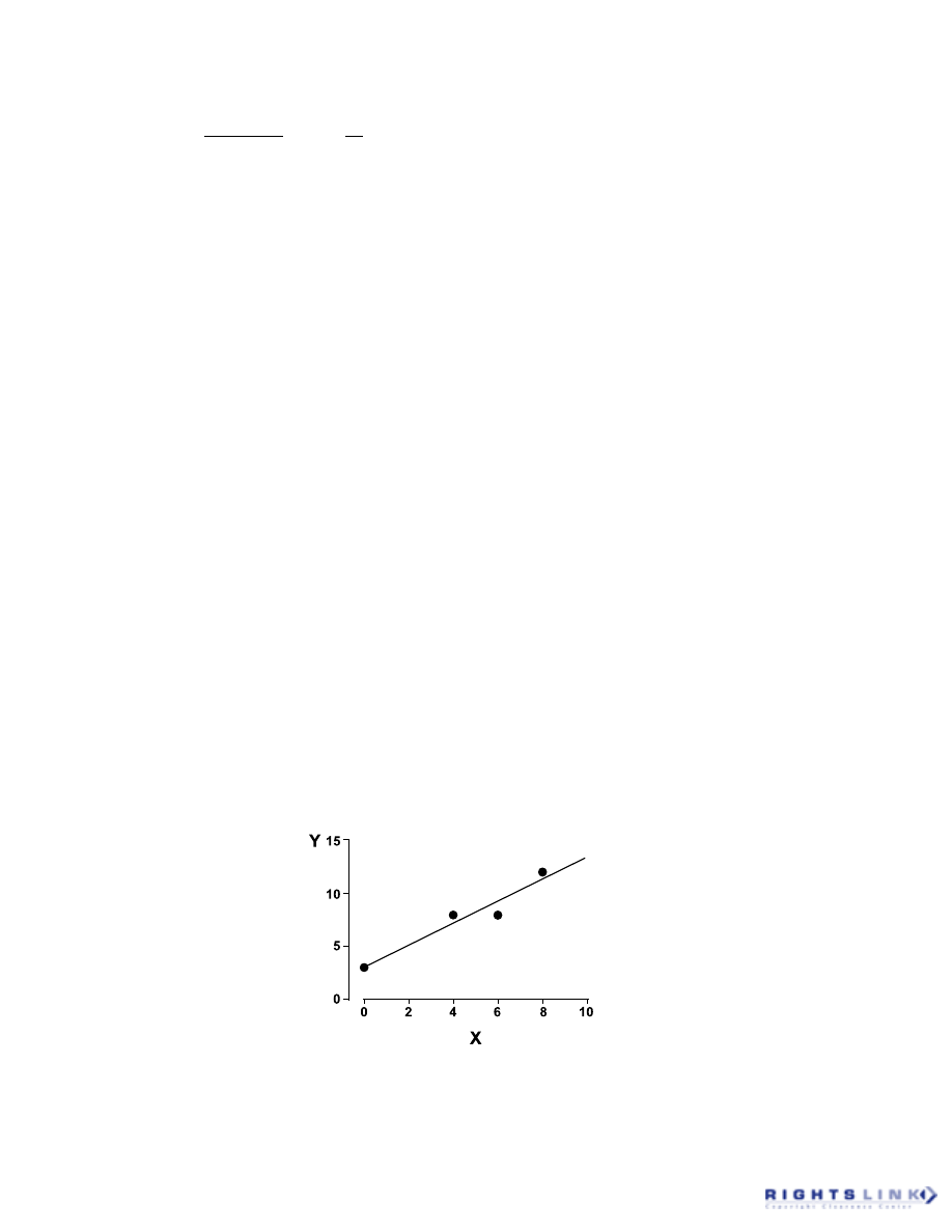
1. The least squares fit of the dataset out-
lined above is shown in Figure 7. Note that
the best-fit straight line yields nonzero re-
siduals for three of the four datapoints. Nev-
ertheless, the resulting line is based on pa-
rameter estimates that give the smallest
sum-of-squares of those residuals.

Why do we use the sum of the square of

the residuals and not another norm of the
deviation, such as the average of the absolute
values of the residuals? Arguably, simply
because of convention! Different norms of
deviation have different relative sensitivities
to small and large deviations and conven-
tional usage suggests that sums of the square
residuals represent a sensible compromise.

4,10

The popularity of least squares estimators
may also be based on the fact that they are
relatively easy to determine and that they are
accurate estimators if certain assumptions are

met regarding the independence of errors and
a Gaussian distribution of errors in the
data.

8,9,11

Nonetheless, for extremely large

deviations due to outlier points, least squares
procedures can fail in providing a sensible fit
of the model to the data.

Although the example used above was

based on a linear model, nonlinear least
squares follow the same principles as linear
least squares and are based on the same
assumptions. The main difference is that the
sum-of-squares merit function for linear
models is well-behaved and can be solved
analytically in one step, whereas for nonlin-
ear models, iterative or numerical proce-
dures must be used instead.

In most common applications of the least

squares method to linear and nonlinear
models, it is assumed that the majority of
the error lies in the dependent variable.
However, there can be circumstances when
both X and Y values are attended by ran-
dom error, and different fitting approaches
are warranted. One such approach has been
described by Johnson,

and is particularly

useful for fitting data to nonlinear models.
In essence, Johnson’s method utilizes a form
of the standard

merit function, given

above, that has been expanded to include
the “best-fit” X value and its associated
variance. The resulting merit function is then
minimized using an appropriate least squares
curve fitting algorithm.

−













∑

(

, )

FIGURE 7. The minimized least squares fit of the straight line model [Equation (2)] to the dataset
shown in Figures 5 and 6.

Critical Reviews in Biochemistry and Molecular Biology Downloaded from informahealthcare.com by 83.26.195.157 on 11/28/10

For personal use only.

371

C. Nonleast Squares

Cornish-Bowden

has listed the mini-

mal requirements for optimal behavior of
the least squares method:

Correct choice of model.

Correct data weighting is known.

Errors in the observations are indepen-
dent of one another.

Errors in the observations are normally
distributed.

Errors in the observations are unbi-
ased (have zero mean).

And we can add:

None or the datapoints are erroneous
(outliers).

Often, however, the requirements for

optimal behavior cannot be met. Other tech-
niques are available for deriving parameter
estimates under these circumstances, and
they are generally referred to as “robust
estimation” or “robust regression” tech-
niques. Because the word “robustness” has
a particular connotation, it is perhaps unfair
to class all of the diverse nonleast squares
procedures under the same umbrella. Over-
all, however, the idea behind robust estima-
tors is that they are more insensitive to de-
viations from the assumptions that underlie
the fitting procedure than least squares esti-
mators.

“Maximum likelihood” calculations are

one class of robust regression techniques
that are not based on a Gaussian distribution
of errors. In essence, regression procedures
attempt to find a set of model parameters
that generate a curve that best matches the
observed data. However, there is no way of
knowing which parameter set is the correct
one based on the (sampled) data, and thus
there is no way of calculating a probability
for any set of fitted parameters being the

“correct set.” Maximum likelihood calcula-
tions work in the opposite direction, that is,
given a particular model with a particular
set of parameters, maximum likelihood cal-
culations derive a probability for the data
being obtained. This (calculated) probabil-
ity of the data, given the parameters, can
also be considered to be the likelihood of
the parameters, given the data.

The goal is

then to fit for a set of parameters that maxi-
mize this likelihood, hence the term “maxi-
mum likelihood,” and the calculations at-
tempt to find the regression that has the
maximum likelihood of producing the ob-
served dataset. It has been pointed out that
there is no formal mathematical basis for
the maximum likelihood procedure and be-
cause maximum likelihood calculations are
quite involved, they are not routinely uti-
lized explicitly.

Fortunately the simpler least

squares methods described above are equiva-
lent to maximum likelihood calculations
where the assumptions of linear and nonlin-
ear regression (particularly the independence
and Gaussian distribution of the errors in
the data) are valid.

8,9,11

Certain robust regression techniques

focus on using measures of central tendency
other than the mean as the preferred statis-
tical parameter estimator. For instance,
Cornish-Bowden

has described how the

median is more insensitive to outlier points
in linear regression and certain cases of
nonlinear regression than the mean. A draw-
back of this approach, however, is that it
quickly becomes cumbersome when ex-
tended to more complex linear problems.

D. Weighting

The simplest minimization functions

make no distinction between different ex-
perimental points, and assume that each
observation contributes equally to the esti-

Critical Reviews in Biochemistry and Molecular Biology Downloaded from informahealthcare.com by 83.26.195.157 on 11/28/10

For personal use only.

372

mation of model parameters. This is appro-
priate when the variance of all the observa-
tions is uniform, and the error is referred to
as homoscedastic. However, in reality it is
common that different points have different
variances associated with them with the re-
sult that the points with the most variance
may have an undue influence on the param-
eters obtained from an unweighted curve
fit. For example, results from many biologi-
cal experiments are often expressed as a
change from a baseline value, with the con-
sequence that the points near the baseline
become small numbers (near zero) with a
low variance. Points representing larger re-
sponses will naturally have a larger vari-
ance, a situation that can be described as
heteroscedasticity. An unweighted curve fit
through heteroscedastic data will allow the
resulting curve to deviate from the well-
defined (tight) near-zero values to improve
the fit of the larger, less well-defined val-
ues. Clearly it would be better to have the fit
place more credence in the more reliably
estimated points, something that can be
achieved in a weighted curve fit.

Equation (13) was used previously to

define the general, least squares, minimiza-
tion function. There are a number of varia-
tions available for this function that employ
differential data weighting.

These func-

tions explicitly define a value for the w

term in Equation (13). For instance, if w

1 or a constant, then the weighting is said to
be “uniform”; if w

= Y

, then

and the weighting is said to be “relative.”
Relative weighting is also referred to as
“weighting by 1/Y

” and is useful where the

experimental uncertainty is a constant frac-
tion of Y. For example, counts of radioac-
tive decay will have variances described by
the Poisson distribution where the variance

scales with the mean, and thus the likely
error in each estimate is a constant percent-
age of counts rather than a constant value
for any number of counts. Thus, a curve fit
allowing for relative weighting can adjust
for the resulting heteroscedastic variance.
Another useful weighting value is
This yields “weighting by 1/Y” and is ap-
propriate, for example, when most of the
experimental uncertainty in the dependent
variable is due to some sort of counting
error.

Other weighting schemes utilize the

number of replicates that are measured for
each value of Y to determine the appropri-
ate weight for the datapoints.

E. Regression Algorithms

What are the actual “mechanics” that

underlie the

minimization process be-

hind least squares regression techniques?
The

merit function for linear models

(including polynomials) is quadratic in
nature, and is thus amenable to an exact
analytical solution. In contrast, nonlinear
problems must be solved iteratively, and
this procedure can be summarized as fol-
lows:

Define the merit function.

Start with a set of initial estimates
(guesses) of the regression param-
eters and determine the value of the
merit function for this set of esti-
mates.

Adjust the parameter estimates and re-
calculate the merit function. If the merit
function is improved, then keep the
parameter values as new estimates.

Repeat step c (each repeat is an “itera-
tion”). When further iterations yield a
negligible improvement in the fit, stop
adjusting the parameter estimates and
generate the curve based on the last set
of estimates.







∑

( )

Critical Reviews in Biochemistry and Molecular Biology Downloaded from informahealthcare.com by 83.26.195.157 on 11/28/10

For personal use only.

373

The rules for adjusting the parameters

of the nonlinear model are based on matrix
algebra and are formulated as computer al-
gorithms. The merit function can be viewed
as a multidimensional surface that has all
possible sum-of-squares values as one plane
and all possible values of each of the model
parameters as the other planes. This surface
may thus vary from a smooth, symmetrical
shape to one characterized by many crests
and troughs. The role of the nonlinear re-
gression algorithm is to work its way down
this surface to the deepest trough that should
then correspond to the set of model param-
eters that yield the minimum sum-of-squares
value.

There are a number of different algo-

rithms that have been developed over the
years, and they all have their pros and cons.
One of the earliest algorithms is the method
of steepest descent (or the gradient search
method

). This method proceeds down the

steepest part of the multidimensional merit
function surface in fixed step lengths that
tend to be rather small.

At the end of each

iteration, a new slope is calculated and the
procedure repeated. Many iterations are re-
quired before the algorithm converges on a
stable set of parameter values. This method
works well in the initial iterations, but tends
to drag as it approaches a minimum value.

The Gauss-Newton method is another

algorithm that relies on a linear approxima-
tion of the merit function. By making this
approximation, the merit function ap-
proaches a quadratic, its surface becomes a
symmetrical ellipsoid, and the iterations of
the Gauss-Newton algorithm allow it to
converge toward a minimum much more
rapidly than the method of steepest descent.
The Gauss-Newton method works best
when it is employed close to the surface
minimum, because at this point most merit
functions are well approximated by linear
(e.g., quadratic) functions.

In contrast, the

Gauss-Newton method can work poorly in

initial iterations, where the likelihood of
finding a linear approximation to the merit
function is decreased.

A method exploiting the best features of

the methods of steepest descent and Gauss-
Newton was described by Marquardt, based
on an earlier suggestion by Levenberg,

and

the resulting algorithm is thus often referred
to as the Levenberg-Marquardt method.
Marquardt realized that the size of the in-
crements in an interative procedure poses a
significant scaling problem for any algo-
rithm, and proceeded to refine the scaling
issue and derive a series of equations that
can approximate the steepest descent method
at early iterations and the Gauss-Newton
method at later stages closer to the mini-
mum. The Levenberg-Marquard method
(sometimes simply referred to as the
Marquardt method) has become one of the
most widespread algorithms used for com-
puterized nonlinear regression.

Another type of algorithm that is geo-

metric rather than numeric in nature is the
Nelder-Mead Variable Size Simplex
method.

8,14

Unlike the methods outlined

above, this method does not require the cal-
culation of any derivatives. Instead, this al-
gorithm depends on the generation of a
number of starting points, called “vertices,”
based on initial estimates for each param-
eter of the model, as well as an initial incre-
ment step. The vertices form a multidimen-
sional shape called a “simplex.” The
goodness of fit is evaluated at each vertex in
the simplex, the worst vertex is rejected and
a new one is generated by combining desir-
able features of the remaining vertices. This
is repeated in an iterative fashion until the
simplex converges to a minimum. The big
advantage of the Nelder-Mead method is
that it is very successful in converging to a
minimum; its main disadvantage is that it
does not provide any information regarding
the errors associated with the final param-
eter estimates.

Critical Reviews in Biochemistry and Molecular Biology Downloaded from informahealthcare.com by 83.26.195.157 on 11/28/10

For personal use only.

374

V. WHEN TO DO IT
(APPLICATION OF CURVE
FITTING PROCEDURES)

A. Calibration Curves (Standard
Curves)

Calibration curves are most convenient

when they are linear, but even for assays
where a linear relationship is expected on
theoretical grounds, nonlinear curves can
result from instrumentation nonlinearities
and other factors. The equation of a curve
fitted through the calibration data will al-
low convenient conversion between the
raw measurement and the required value.
In cases where there is no theoretical ba-
sis for choosing one model over another,
calibration curves can be considered to be
a smoothing rather than a real fitting prob-
lem and one might decide to apply a poly-
nomial model to the data because of the
availability of an analytical solution. In
such a case the order of the chosen poly-
nomial would need to be low so that noise
in the calibration measurements is not
converted into wobbles on the calibration
curve.

B. Parameterization of Data
(Distillation)

It is often desirable to describe data in

an abbreviated way. An example of this is
the need to summarize a concentration–re-
sponse curve into a potency estimate and
maximum response value. These parameters
are easily obtained by eyeballing the data,
but an unbiased estimate from an empirical
curve fit is preferable and probably more
acceptable to referees!

VI. HOW TO DO IT

A. Choosing the Right Model

1. Number of Parameters

The expectation function should include

the minimum number of parameters that
adequately define the model and that allow
for a successful convergence of the fit.

If a model is overparameterized, it is

considered to possess “redundant” param-
eters (often used interchangeably with the
term “redundant variables”), and the regres-
sion procedure will either fail or yield mean-
ingless parameter estimates. Consider the
“operational model” of Black and Leff.

This is a model that is often used in pharma-
cological analyses to describe the concen-
tration–response relationship of an agonist
(A) in terms of its affinity (dissociation
constant) for its receptor (K

), its “opera-

tional” efficacy (

), and the maximum re-

sponse (E

) that the tissue can elicit. One

common form of the model is:

(14)

where E denotes the observed effect. Figure
8 shows a theoretical concentration–response
curve, plotted in semilogarithmic space, that
illustrates the relationship between the op-
erational model parameters and the maxi-
mal asymptote (

) and midpoint location

(EC

) of the resulting sigmoidal curve. A

concentration–response curve like the one
in Figure 8 can be successfully fitted using
the two-parameter version of the Hill equa-
tion, which describes the curve in terms of
only the EC

and

(the slope being equal

to 1):

(15)

⋅ ⋅

+ ⋅

[ ]

([ ]

)

[ ]

⋅

[ ]

Critical Reviews in Biochemistry and Molecular Biology Downloaded from informahealthcare.com by 83.26.195.157 on 11/28/10

For personal use only.

375

However, it can be seen in Figure 8 that

the midpoint and maximal asymptote of the
curve are related to the operational model in
a more complicated manner; each param-
eter of the sigmoidal Hill equation is com-
prised of two operational model parameters.
If someone were to try directly fitting Equa-
tion (14) to this curve in order to derive
individual estimates of E

, K

, and

, they

would be unsuccessful. As it stands, the
operational model is overparameterized for
fitting to a single curve; the regression algo-
rithm simply will not be able to apportion
meaningful estimates between the individual
operational model parameters as it tries to
define the midpoint and maximal asymptote
of the concentration–response curve. In prac-
tice, the successful application of the opera-
tional model to real datasets requires addi-
tional experiments to be incorporated in the
curve fitting process that allow for a better
definition of the individual model param-
eters.

16,17

2. Shape

When fitting empirical models to data

the most important feature of the model
must be that its shape should be similar to
the data. This seems extraordinarily obvi-
ous, but very little exploration of the litera-

ture is needed to find examples where the
curve and the data have disparate shapes!
Empiricism allows one a great deal of free-
dom in choosing models, and experiment-
ers should not be overly shy of moving
away from the most common models (e.g.,
the Hill equation) when their data ask for it.
Even for mechanistic models it is important
to look for a clear shape match between the
model and data: a marked difference can
only mean that the model is inappropriate or
the data of poor quality.

Perhaps the only feature that practi-

cally all biological responses have in com-
mon is that they can be approximated by
nonlinear, saturating functions. When plot-
ted on a logarithmic concentration scale,
responses usually lie on a sigmoid curve,
as shown in Figures 71 and 8, and a num-
ber of functions have been used in the past
to approximate the general shape of such
responses. Parker and Waud,

for instance,

have highlighted that the rectangular hy-
perbola, the integral of the Gaussian distri-
bution curve, the arc-tangent, and the lo-
gistic function have all been used by various
researchers to empirically fit concentra-
tion–response data. Some of these func-
tions are more flexible than others; for in-
stance, the rectangular hyperbola has a fixed
slope of 1. In contrast, the logistic equation
has proven very popular in the fitting of
concentration–response data:

FIGURE 8. The relationship between the Hill equation [Equation (15)] parameters, a and EC

, and

the operational model [Equation (14)] parameters K

, t, and E

, in the description of a concentra-

tion–response curve of an agonist drug. It can be seen that each parameter of the Hill equation is
composed of two operational model parameters.

Critical Reviews in Biochemistry and Molecular Biology Downloaded from informahealthcare.com by 83.26.195.157 on 11/28/10

For personal use only.

376

(16)

Part of the popularity of this equation

is its flexibility and its ability to match the
parameters of the Hill equation [Equation
(1)] for empirical fitting purposes.

In general, the correct choice of expecta-

tion function is most crucial when fitting
mechanistic models. The difficulty in ascer-
taining the validity of the underlying model
in these cases arises because the curve fitting
process is undertaken with the automatic as-
sumption that the model is a plausible one
prior to actually fitting the model and apply-
ing some sort of diagnostics to the fit (see
Assessing the Quality of the Fit, below). We
must always remain aware, therefore, that
we will never really know the “true” model,
but can at least employ a reasonable one that
accommodates the experimental findings and,
importantly, allows for the prediction of test-
able hypotheses. From a practical standpoint,
this may be seen as having chosen the “right”
mechanistic model.

3. Correlation of Parameters

When a model, either mechanistic or

empirical, is applied to a dataset we gener-

ally consider each of the parameters to be
responsible for a single property of the curve.
Thus, in the Hill equation, there is a slope
parameter, S, a parameter for the maximum
asymptote (

), and a parameter for the loca-

tion (K or EC

). Ideally, each of these pa-

rameters would be entirely independent so
that error or variance in one does not affect
the values of the others. Such a situation
would mean that the parameters are entirely
uncorrelated. In practice it is not possible to
have uncorrelated parameters (see Figure
9), but the parameters of some functions are
less correlated than others. Strong correla-
tions between parameters reduce the reli-
ability of their estimation as well as making
any estimates from the fit of their variances
overly optimistic.

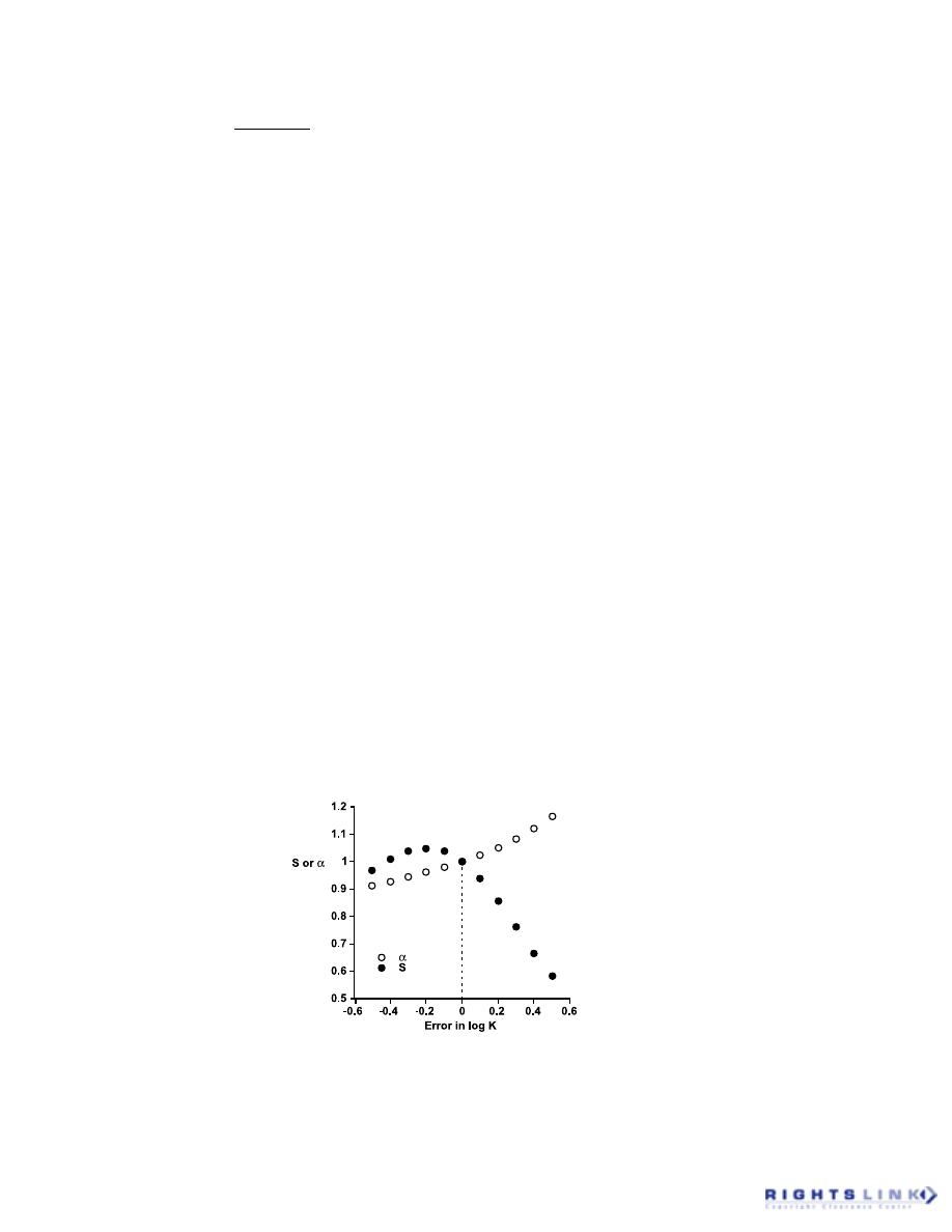
4. Distribution of Parameters

The operational model example can also

be used to illustrate another practical con-
sideration when entering equations for curve
fitting,

namely

the

concept

“reparameterization.”

When fitting the

operational model or the Hill equation to
concentration–response curves, the param-
eters may be entered in the equation in a
number of ways; for instance, the EC

− +

(

)

α β

FIGURE 9. Altered estimates of the maximal asymptote, a, and the slope, S, obtained by fitting the
Hill equation to logistic data where the parameter K (log K) was constrained to differ from the correct
value. The systematic relationship between the error in K and the values of the parameters S and

indicates that each is able to partially correct for error in K and thus are correlated with K.

Critical Reviews in Biochemistry and Molecular Biology Downloaded from informahealthcare.com by 83.26.195.157 on 11/28/10

For personal use only.

377

commonly entered as 10

LogEC50

. This

reparameterization means that the regres-
sion algorithm will actually provide the best-
fit estimate of the logarithm of the EC

Why reparameterize? As mentioned earlier,
many of the assumptions of nonlinear re-
gression rely on a Gaussian distribution of
experimental uncertainties. Many model
parameters, including the EC

of the Hill

equation, the dissociation constant of a hy-
perbolic radioligand binding equation, and
the

parameter of the operational model,

follow an approximately Gaussian distribu-
tion only when transformed into loga-
rithms.

Thus, although not particularly

important for the estimation of the paramet-
ric value, reparameterization can improve
the validity of statistical inferences made
from nonlinear regression algorithms.

Other examples of reparameterizations that
can increase the statistical reliability of the
estimation procedure include recasting time
parameters as reciprocals and counts of ra-
dioactive decay as square roots.

B. Assessing the Quality of the
Fit

The final determination of how “appro-

priate” the fit of a dataset is to a model will
always depend on a number of factors, in-
cluding the degree of rigor the researcher
actually requires. Curve fitting for the de-
termination of standard curves, for instance,
will not warrant the same diagnostic criteria
one may apply to a curve fit of an experi-
mental dataset that was designed to investi-
gate a specific biological mechanism. In the
case of standard curves, an eyeball inspec-
tion of the curve superimposed on the data
is usually sufficient to indicate the reliabil-
ity of the fit for that specific purpose. How-
ever, when the fitting of models to experi-
mental data is used to provide insight into
underlying biological mechanisms, the abil-

ity to ascribe a high degree of appropriate-
ness to the resulting curve fit becomes para-
mount.

1. Inspection

Although usually sufficient for empiri-

cal models, an initial test for conformity of
the data to any selected model is a simple
inspection of the curve fit superimposed on
the data. Although rudimentary, this proce-
dure is quite useful in highlighting really
bad curve fits, i.e., those that are almost
invariably the consequence of having inad-
vertently entered the wrong equation or set-
ting certain parameter values to a constant
value when they should have been allowed
to vary as part of the fitting process. Assum-
ing that visual inspection does not indicate
a glaring inconsistency of the model with
the data, there are a number of statistical
procedures that can be used to quantify the
goodness of the fit.

2. Root Mean Square

Figure 10 shows a schematic of an ex-

perimental dataset consisting of 6 observa-
tions (open circles labeled obs1 – obs6) and
the superimposed best-fit of a sigmoidal
concentration–response model [Equation
(15)] to the data. The solid circles (exp1 –
exp6) represent the expected response cor-
responding to each X-value used for the
determination of obs1 – obs6, derived from
the model fit. The sum of the squared re-
siduals, i.e., the sum of the squared differ-
ences between the observed and expected
responses has also been defined as the Er-
ror Sum of Squares (SSE), and it is this
quantity that most researchers think of when
discussing the sum-of-squares derived from
their curve fitting exercises [see Equation
(13)]:

Critical Reviews in Biochemistry and Molecular Biology Downloaded from informahealthcare.com by 83.26.195.157 on 11/28/10

For personal use only.

378

SSE = (obs1 – exp1)

+ (obs2 – exp2)

+ …

+ (obs6 – exp6)

(17)

The SSE is sometimes used as an index

of goodness-of-fit; the smaller the value,
the better the fit. However, in order to use
this quantity more effectively, an allowance
must also be made for the “degrees of free-
dom” of the curve fit. For regression proce-
dures, the degrees of freedom equal the to-
tal number of datapoints minus the number
of model parameters that are estimated. In
general, the more parameters that are added
to a model, the greater the likelihood of
observing a very close fit of the regression
curve to the data, and thus a smaller SSE.
However, this comes at the cost of degrees
of freedom. The “mean square error” (MSE)
is defined as the SSE divided by the degrees
of freedom (df):

(18)

Finally, the square root of MSE is equal to
the root mean square, RMS:

(19)

The RMS (sometimes referred to as S

y.x

)

is a measure of the standard deviation of the
residuals. It should be noted, however, that
although RMS is referred to as the “stan-

dard deviation” or “standard error” of the
model, this should not be confused with the
standard deviation or error associated with
the individual parameter estimates. The de-
gree of uncertainty associated with any
model parameter is derived by other meth-
ods (see below).

3. R

(Coefficient of Determination)

Perhaps more common than the RMS,

the R

value is often used as a measure of

goodness of fit. Like the r

value from

linear regression or correlation analyses,
the value of R

can range from 0 to 1; the

closer to 1 this value is, the closer the
model fits the dataset. To understand the
derivation of R2, it is important to first
appreciate the other “flavors” of sums-of-
squares that crop up in the mathematics of
regression procedures in addition to the
well-known SSE.

Using Figure 10 again as an example,

the sum of the squared differences between
each observed response and the average of
all responses (obsav) is defined as the Total
Sum of Squares (SST; sometimes denoted
as Syy):

SST = (obs1 – obs

)

+ (obs2 – obs

)

+ …

+ (obs6 – obs

)

(20)

FIGURE 10. Relationship between a set of experimental observations (open circles; obs1 – obs6)
and their corresponding least squares estimates (solid circles; exp1 – exp6). The horizontal dashed
line represents the average of all the experimental observations (obs

MSE

SSE

RMS

SSE

Critical Reviews in Biochemistry and Molecular Biology Downloaded from informahealthcare.com by 83.26.195.157 on 11/28/10

For personal use only.

379

where

obs

= (obs1 + obs2 + obs3 + obs4 + obs5

+ obs6)/6

(21)

The sum of the squared differences be-

tween each estimated (expected) response,
based on the model, and the average of all
observed responses is defined as the Re-
gression Sum of Squares (SSR):

SSR = (exp1 – obs

)2 + (exp2 – obs

)2 +

… + (exp6 – obs

(22)

The total sum of squares, SST, is equal

to the sum of SSR and SSE, and the goal of
regression procedures is to minimize SSE
(and, as a consequence, SST).

Using the definitions outlined above,

the value of R

can be calculated as fol-

lows:

5,10

(23)

is the proportion of the adjusted variance

in the dependent variables that is attributed
to (or explained by) the estimated regres-
sion model. Although useful, the R

value is

often overinterpreted or overutilized as the
main factor in the determination of good-
ness of fit. In general, the more parameters
that are added to the model, the closer R

will approach a value of 1. It is simply an
index of how close the datapoints come to
the regression curve, not necessarily an in-
dex of the correctness of the model, so while
R

may be used as a starting point in the

assessment of goodness of fit, it should be
used in conjunction with other criteria.

4. Analysis of Residuals

Because the goal of least squares re-

gression procedures is to minimize the sum

of the squares of the residuals, it is not
surprising that methods are available for
analyzing the final residuals in order to as-
sess the conformity of the chosen model to
the dataset. The most common analysis of
residuals relies on the construction of a scat-
ter diagram of the residuals.

13,20

Residuals

are usually plotted as a function of the val-
ues of the independent variable. If the model
is adequate in describing the behavior of the
data, then the residuals plot should show a
random scatter of positive and negative re-
siduals about the regression line. If, how-
ever, there is a systematic deviation of the
data from the model, then the residuals plot
will show nonrandom clustering of positive
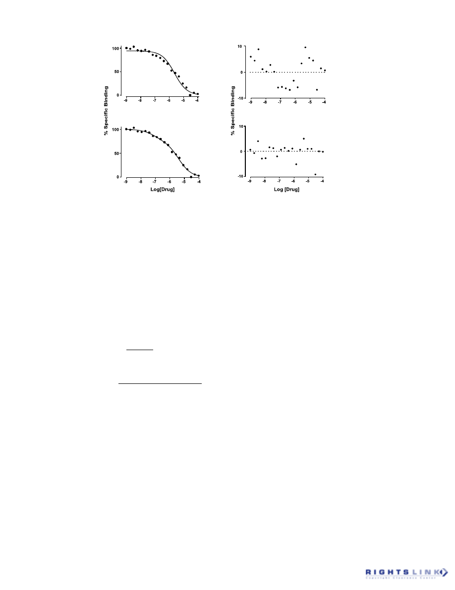
and negative residuals. Figure 11 illustrates
this with an example of a radioligand com-
petition binding experiment. When the data
are fitted to a model of binding to a single
site, a systematic deviation of the points
from the regression curve is manifested as
clustering in the residuals plot. In contrast,
when the same dataset is fitted to a model of
binding to two sites, a random scatter of the
residuals about the regression line indicates
a better fit of the second model. This type of
residual analysis is made more quantitative
when used in conjunction with the “runs
test” (see below).

There are many other methods of per-

forming detailed analyses of residuals in
addition to the common method described
above. These methods include cumulative
probability distributions of residuals,

tests,

and a variety of tests for serial correla-
tion.

7,10,11,20

5. The Runs Test

The runs test is used for quantifying

trends in residuals, and thus is an additional
measure of systematic deviations of the
model from the data. A “run” is a consecu-

SSR

SST

SSE

SST

= −

Critical Reviews in Biochemistry and Molecular Biology Downloaded from informahealthcare.com by 83.26.195.157 on 11/28/10

For personal use only.

380

tive series of residuals of the same sign
(positive or negative). The runs test involves
a calculation of the expected number of
runs, given the total number of residuals
and expected variance.

The test uses the

following two formulae:

(24)

(25)

where N

and N

denote the total number of

positive and negative residuals, respectively.
The results are used in the determination of
a P value.

5,13

A low P value indicates a sys-

tematic deviation of the model from the data.
In the example shown in Figure 11, the one-
site model fit was associated with a P value
of less than 0.01 (11 runs expected, 4 ob-
served), whereas the two-site model gave a P
value of 0.4 (10 runs expected, 9 observed).

C. Optimizing the Fit

With the ubiquitous availability of pow-

erful computers on most desktops, the im-
pressive convergence speed of modern curve
fitting programs can often lead to a false
sense of security regarding the reliability of
the resulting fit. Assuming that the appro-
priate model has been chosen, there are still
a number of matters the biomedical investi-
gator must take into account in order to
ensure that the curve fitting procedure will
be optimal for their dataset.

1. Data Transformations

Most standard regression techniques as-

sume a Gaussian distribution of experimen-
tal uncertainties and also assume that any
errors in Y and X are independent. As men-
tioned earlier, however, these assumptions
are not always valid. In particular, the vari-
ance in the experimental dataset can be

FIGURE 11. An example of residuals plots. The top panel represents a curve fit based on a one
binding site model to a data set obtained from a radioligand competition binding assay (left) and
its corresponding residuals plot (right). Note the clustering of positive and negative residuals. The
bottom panel represents a curve fit based on a two binding site model to the same dataset (left)
and its corresponding residuals plot (right). Note the random scatter of positive and negative
residuals in this case.

Expected Runs

N N

Expected Variance

−

N N

(

)

(

) (

)

Critical Reviews in Biochemistry and Molecular Biology Downloaded from informahealthcare.com by 83.26.195.157 on 11/28/10

For personal use only.

381

heteroscedastic, that is, it changes in a sys-
tematic fashion with the variables. One
method for optimizing the curve fitting pro-
cess to adjust for heteroscedastic errors is to
weight the data, as discussed earlier, while
another approach is to transform the data to
a form where the errors become more
homoscedastic prior to the application of the
regression technique. Transformations such
as the square root or logarithm of the depen-
dent or independent variables do not neces-
sarily cause any problems of their own, pro-
vided they reduce rather than increase any
heteroscedasticity in the data. In contrast,
classical “linearising” transformations, where
a new variable is derived from both the origi-
nal dependent and independent variables, are
quite dangerous and it is unfortunate that
they are still common practice in some labo-
ratories. Indiscriminate data transforms of
the latter kind are troublesome because they
have the potential of distorting homoscedastic
errors in experimental uncertainties and thus
violating the assumptions of any subsequent
regression procedure. Transforms are appro-
priate if they have a normalizing effect on
heteroscedastic errors; they are not valid oth-
erwise. In addition, some data transforms,
embodied in reciprocal plots (e.g.,
Lineweaver-Burk) or the Scatchard transfor-
mation, violate the assumption of indepen-
dence between X and Y variables and are
equally inappropriate. In contrast, transfor-
mation of model parameters (as described
earlier) may often have an optimising effect
on the fitting procedure.

2. Initial Estimates

All curve fitting algorithms require the

specification of initial estimates of the pa-
rameters that are then optimized to yield the
best fit. No regression algorithm is perfect,
and failure to specify reasonable parameter
estimates may result in a failure of the algo-

rithm to converge or, more insidiously, a
convergence of the curve fit on a “local
minimum.” If we recall our earlier discus-
sion of the surface of the merit function that
the various algorithms travel down, it is
possible to envisage a multiparameter model
that results in a series of troughs such that
the algorithm may settle in one as if it has
converged on the best fit when, in fact, a
deeper trough is available elsewhere on the
merit function surface. This is an example
of the program converging on a local mini-
mum (Figure 12), where the curve fit is not
optimal although the user may think that the
best fit has been obtained. The best safe-
guard against this problem is to perform the
regression analysis a number of times using
different initial estimates. A well-behaved
model should converge on essentially the
same final estimates each time.

Some commercial programs make the

process of finding initial parameter estimates
relatively painless by incorporating approxi-
mate rules that find initial estimates for the
user. Although this is expedient, there is no
substitute for the researcher personally ad-
dressing the issue of initial parameter esti-
mates. This forces one to focus on the un-
derlying model and the meaning of the model
parameters, and it is then not too difficult to
come up with a best guess. If further assis-
tance is required, or if there are some pa-
rameters that the user does not have a par-
ticular “feel” for, then a simplex algorithm
or a Monte Carlo-based algorithm (see be-
low) may be utilized to derive estimates that
can subsequently be improved upon by the
more standard derivative-based algorithms.

D. Reliability of Parameter
Estimates

The determination of the reliability of

the estimated parameters derived from a
curve fit is as important as the actual esti

Critical Reviews in Biochemistry and Molecular Biology Downloaded from informahealthcare.com by 83.26.195.157 on 11/28/10

For personal use only.

382

mation of the parametric values themselves.
All known methods for the calculation of
standard errors and confidence intervals
from regression algorithms are based on
the mathematics of linear models. Since
nonlinear models are more common in bi-
ology than linear models, it is perhaps dis-
heartening to have to accept that there are
no exact theories for the evaluation of para-
metric errors in nonlinear regression. How-
ever, there are a number of procedures
available for approximating these errors
such that, in most practical applications, a
reasonable measure of parameter error is
obtained.

1. Number of Datapoints

The number of experimental datapoints

collected and analyzed will play a crucial
role in the curve fitting process in one (or
both) of two ways:

Determination of the appropriateness
of the model.

Determination of the accuracy of the
parameter estimates.

Different measures for goodness-of-fit

have already been covered, but some dis-
cussion on the influence of datapoint num-

ber is also warranted at this point, since it

can form an important component of choos-
ing the right model, that adequately accounts
for the data. Figure 13 illustrates the effect
of datapoint number on one of the most
common statistical procedures utilized in
discriminating between variants of the same
model, i.e., the “F-test” (or “extra-sum-of-
squares” test). The actual test is described
in greater detail in the next section. For
now, it is sufficient to point out that the F-
test relies heavily on the degrees of freedom
associated with the fit to any model, which
are in turn dependent on the number of
datapoints minus the number of parameters
estimated. Although all the points in each of
the panels in Figure 13 are taken from the
same simulated dataset, the “correct” model
(a two binding site model) can only be sta-
tistically resolved when the datapoints were
increased from 6 (panel A) or 10 (panel B),
to 20 (panel C).

Assuming that the researcher has a

priori reasons for deciding that a particu-
lar model is most appropriate under their
circumstances, the number of datapoints
will still be crucial in determining the
accuracy of the parameters based on that
model. Table 1 lists the parameter esti-
mates and corresponding 95% confidence
intervals of a two binding site model (i.e.,
the correct model) applied to the datasets

FIGURE 12. Multiple minima in parameter space. The best fit is obtained at that set of parameter
values yielding the smallest possible sum of squares. Depending on the initial estimates, however,
the fitting algorithm may converge on parameter sets which, although yielding a reduced sum of
squares, do not correspond to the minimum possible sum of squares. The regression is then said
to have converged on a “local minimum.”

Critical Reviews in Biochemistry and Molecular Biology Downloaded from informahealthcare.com by 83.26.195.157 on 11/28/10

For personal use only.

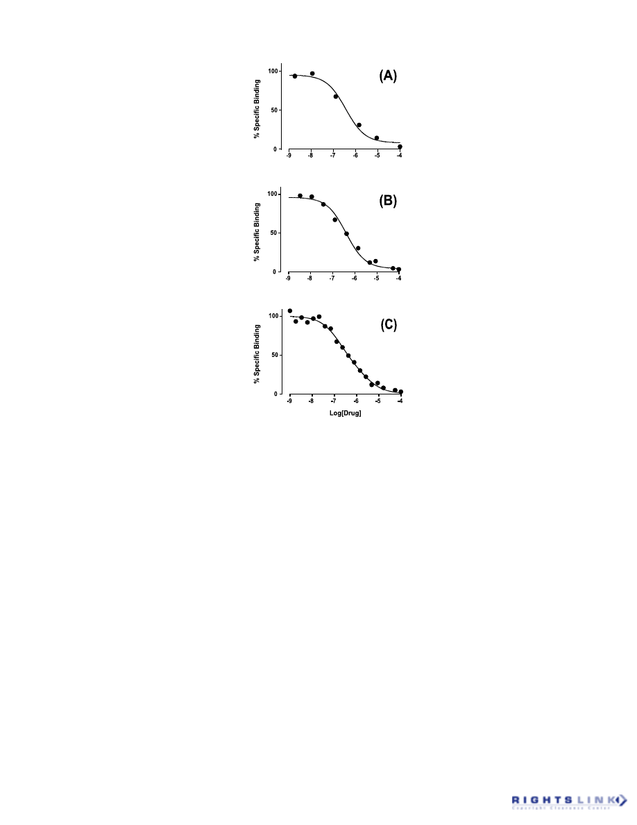
383

of Panel A and Panel C, respectively, of
Figure 13. Although the final parameter
estimates appear comparable in each in-
stance, the fit based on the small number
of datapoints is associated with unaccept-
ably large confidence intervals. There are
simply not enough points to accurately
define all the parameters of the model. In
contrast, increasing the number of
datapoints to 20 allowed for reasonable
estimates of the error associated with each
parameter estimate. The confidence inter-
vals reported in the table were calculated
from the asymptotic standard errors de-

rived by the computer program from the
fitting algorithm and are most likely un-
derestimates of the true error (see below),
thus rendering our (already shaken) con-
fidence in the accuracy
of minimal-data-point parameter esti-
mates virtually nonexistent. There have
been some methods presented in the lit-
erature for maximizing the reliability of
parameter estimates under conditions of
minimal datapoint number (e.g., Refer-
ences 21 and 22), but there really is no
substitute for a good sampling of experi-
mental datapoints.

FIGURE 13. Influence of data point number on choice of model. The radioligand competition
binding curves above were simulated (with random error) according to a model for binding to two-
sites. The sampling of points in each of the panels is from exactly the same simulated dataset. The
curves in each panel are the least squares fit of the data to either a one- or two-site binding model,
as determined by an F-test (see Section VI. E). Panels A (6 points) and B (10 points) were not
statistically significant from a one-site model. Only in panel C (20 points) were the data able to be
statistically resolved into the (correct) two-site model fit.

Critical Reviews in Biochemistry and Molecular Biology Downloaded from informahealthcare.com by 83.26.195.157 on 11/28/10

For personal use only.

384

2. Parameter Variance Estimates
from Repeated Experiments

The most straightforward and conser-

vative approach to building up an error
profile of a given parameter is to simply
repeat the same experiment many times,
obtain single parameter estimates from each
individual curve fit, and then derive the
mean and standard deviation (and error) of
the parameters using standard textbook
methods. Assuming that each curve fit is
performed under optimal conditions, e.g.,
appropriate number of datapoints, appro-
priate transformation and weighting, etc.,
biomedical research is still fraught with
small overall sample sizes; it is not uncom-
mon to see n = 3 – 6 given in many publi-
cations as the number of times an experi-
ment is repeated. As such, the conservative,
albeit straightforward approach to param-
eter error estimation just described may
not have the power to resolve small differ-

ences between experimental treatments, as
it is based on small sample sizes and, fur-
thermore, does not utilize all the available
datapoints. The remaining methods for
parameter error estimation utilize all the
datapoints in some form or other.

3. Parameter Variance
Estimates from Asymptotic
Standard Errors

The standard errors reported by practi-

cally all commercially available least squares
regression programs fall under this category.
Asymptotic

standard

errors

are

computationally the easiest to determine and,
perhaps not surprisingly, the least accurate.
In most instances, these standard errors will
underestimate the true error that is likely to
be associated with the parameter of interest.

The calculation of the asymptotic stan-

dard error and associated confidence inter-

Table 1
Parameter Estimates and Associated Confidence Intervals from Fitting a Two-Site Model
of Radioligand Competition Binding to Different Data Point Numbers Taken from the
Same Dataset (Panels A and C; Figure 13)

Parameter

Estimate

95% Confidence Interval

Datapoints = 6

Maximum Asymptote

–96.7

45.6 to 148.3

Minimum Asymptote

1.3

–84.8 to 87.56

Log IC50High

–6.7

–9.93 to –3.53

Log IC50Low

–5.1

–16.1 to 5.9

Fraction High

0.74

–1.4 to 2.9

Datapoints = 20

Maximum Asymptote

99.9

95.4 to 104.4

Minimum Asymptote

0.9

–5.5 to 7.4

Log IC

50High

–6.8

–7.3 to –6.5

Log IC

50Low

–5.6

–6.4 to –4.6

Fraction High

0.64

0.4 to 0.8

Y-axis value in the absence of competing drug.

Y-axis value in the presence of saturating concentrations of competing drug.

Potency estimate for competition at the high affinity binding site.

Potency estimate for competition at the low affinity binding site.

Fraction of high affinity binding sites.

Critical Reviews in Biochemistry and Molecular Biology Downloaded from informahealthcare.com by 83.26.195.157 on 11/28/10

For personal use only.

385

vals involves matrix algebra, but may be
summarized as follows:

Determine the Hessian (or “informa-
tion”) matrix. This is the matrix con-
taining the second derivatives of the
parameters with respect to the mini-
mized

merit function.

Evaluate the variance-covariance ma-
trix by multiplying the inverse of the
Hessian matrix by the variance of the
residuals of the curve fit.

The diagonal elements of the resulting
variance-covariance matrix are the
squares of the asymptotic standard er-
rors; the off-diagonal elements of the
matrix are the covariances of the pa-
rameters, and are a measure of the
extent to which the parameters in the
model are correlated with one another.

The computer program then reports the

resulting standard errors. For these errors to
actually be a good measure of the accuracy
of the parameter estimates, the following
assumptions must hold:

The fitting equation is linear.

The number of datapoints is very large.

The covariance terms in the variance-
covariance matrix are negligible.

For nonlinear models, the first assump-

tion is invalid, however, the impact of fail-
ure to conform to this assumption may be
lessened for models that are well behaved,
e.g., contain conditionally linear parameters
or can be approximated by linear functions.
The second assumption can also be reason-
able provided the experimenter is able to
ensure an adequate sampling of datapoints.
Unfortunately, the third assumption is al-
most never realized. As described earlier,
most parameters in nonlinear models show
some degree of correlation with one an-
other; indeed, high correlations are indica-
tive of parameter redundancies in the model.

As such, ignoring the covariances from the
variance-covariance matrix in the reporting
of parameter errors will underestimate the
true error.

Nevertheless, asymptotic standard er-

rors may serve a useful diagnostic role. Since
they will invariably be underestimates of
the true error, very large standard errors or
confidence intervals reported after a curve
fit are indicative of a very poor fit of the
associated parameter (see Table 1). This
may occur, for instance, because the param-
eter is ill defined by the available data.

4. Monte Carlo Methods

The most reliable method for the deter-

mination and validation of model parameter
confidence intervals is also the most com-
puter-intensive. Monte Carlo simulations in-
volve the generation of multiple (hundreds to
thousands) of pseudodatasets, based on a
chosen model, and the subsequent analysis
of the simulated datasets with the same model
used to generate them followed by construc-
tion of a frequency histogram showing the
distribution of parameter estimates.

17,24

Fig-

ure 14 shows a flowchart summarizing the
general approach to Monte Carlo simulation.

The crucial factor in the implementation

of the Monte Carlo approach is the ability to
add random “error” to the pseudodataset
points that accurately reflects the distribution
of experimental uncertainties associated with
the determination of “real” datasets. The best
determinant of this error is the variance of
the fit of the chosen model to real experimen-
tal data, provided that the standard assump-
tions underlying least squares regression
analyses are valid. In addition to the appro-
priate choice of variance for the simulations,
other key features in this approach are the
choice and the number of independent vari-
ables, which again should match those deter-
mined in a typical experiment.

Critical Reviews in Biochemistry and Molecular Biology Downloaded from informahealthcare.com by 83.26.195.157 on 11/28/10

For personal use only.

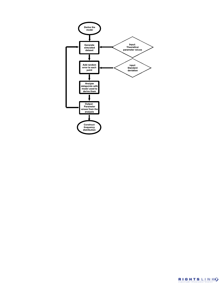
386

The beauty of the Monte Carlo approach

is that the level of accuracy with regard to
the confidence interval profiles is very much
in the hands of the researcher; the greater
the number of simulated datasets, the greater
the resolution of the confidence intervals.
However, this comes at the expense of com-
puter time; a Monte Carlo simulation of
1000 datasets may take 1000 times longer
than a least squares fit of the actual experi-
mental dataset used to pattern the simula-
tions. Coupled with the fact that many com-
mercially available curve fitting packages
do not contain Monte Carlo-compatible pro-
gramming features, the time factor involved
in generating parameter confidence inter-
vals from the Monte Carlo approach dis-
suades many researchers from routinely
using this method. Nonetheless, great in-
sight can be gained from Monte Carlo ap-
proaches. For instance, in addition to pro-
viding the greatest degree of accuracy in

parameter error estimation, Monte Carlo
methods can also guide the experimenter
toward the most appropriate model
reparameterizations in order to optimize the
actual curve fitting procedure.

One potential problem with the stan-

dard Monte Carlo approach is that it is nec-
essary to define the population distributions
for the errors applied to the datapoints. A
normal distribution is most commonly used,
but it is not always clear that it is appropri-
ate. The bootstrap, described below, explic-
itly overcomes that problem.

5. The Bootstrap

“Bootstrapping” is an oddly-named pro-

cess that allows an approximate reconstruction
of the parameters of the population from which
the data have been (at least conceptually)

FIGURE 14. A general approach to Monte Carlo simulation.

Critical Reviews in Biochemistry and Molecular Biology Downloaded from informahealthcare.com by 83.26.195.157 on 11/28/10

For personal use only.

387

sampled.

Bootstrapping differs from standard

Monte Carlo methods in that it makes no as-
sumption about the form of the population, and
instead assumes that the best estimate of the
properties of the population is the experimen-
tally determined dataset. The population is re-
constructed by repeated resampling of the
datapoints to give a large number (hundreds or
even thousands) of new pseudodatasets. The
resampling is done “with replacement,” which
is to say that any particular real datapoint can
appear in each pseudodataset more than one
time. The result is a population of pseudodatasets
that represents a pseudo-population that has
approximately the same properties as the origi-
nal population.

Bootstrapping can be used in several

ways relevant to model fitting. First, it can
provide a pseudopopulation of any param-
eter calculable from each pseudodataset.
Thus it can be used to give confidence inter-
vals for fitted parameters obtained from
methods that do not directly provide esti-
mates of parameter variance, such as the
simplex method. Similarly, it has been used
to estimate the reliability of the variance
estimates obtained from other methods that
rely on the covariance matrix.

Bootstrapping is not without poten-

tial problems. One arises from the fact
that the real dataset is unlikely to include
any samples from the extreme tails of the
overall population of possible datapoints.
This means that bootstrapped populations
generally have less area under the ex-
treme tails than the real population from
which the data were sampled. There are
corrections that can be applied,

but

bootstrapping is not universally accepted
by statisticians.

6. Grid Search Methods

Another computer-intensive approach to

error determination involves the construc-

tion of multidimensional grids based on
model parameter values and then “search-
ing” for those parameter value combina-
tions where the variance of the overall fit
increases significantly. The confidence in-
tervals are then defined as those regions of
the grid (which resemble a multidimensional
ellipsoid) that surround the minimum over
which the variance does not change signifi-
cantly.

8,23

7. Evaluation of Joint
Confidence Intervals

As discussed earlier, the parameters

in most models tend to show some corre-
lation with one another. The evaluation of
joint confidence intervals is a procedure
that is designed to include the covariance
of the parameters in the determination of
parameter error estimates.

8,13

The equa-

tions underlying this approach, however,
assume that the fitting equation is linear
in order to derive a symmetrical ellipti-
cally-shaped confidence interval profile
of parameters. Unfortunately, this method
yields asymmetric confidence regions for
those nonlinear models that cannot ap-
proximate to a linear model, and is thus
not as reliable as Monte Carlo or Grid
search methods.

E. Hypothesis Testing

Often, the desire to ascertain the stan-

dard error or confidence interval associ-
ated with model parameters is a prelude to
the statistical testing of the parameters ac-
cording to a particular hypothesis. There-
fore, some objective statistical test is re-
quired in order to allow for comparisons
between parameters or comparisons be-
tween models.

Critical Reviews in Biochemistry and Molecular Biology Downloaded from informahealthcare.com by 83.26.195.157 on 11/28/10

For personal use only.

388

1. Assessing Changes in a
Model Fit between Experimental
Treatments

There are three broad approaches to

performing statistical comparisons be-
tween the same model parameters before
and after an experimental treatment. The
first relies on the use of standard paramet-
ric tests, such as the Student’s t-test. The
second approach relies on more computer-
intensive, but preferable comparisons be-
tween parameters based on permutation
tests. The third approach differs from the
other two in that it uses all the experimen-
tal data generated before and after a par-
ticular treatment in a comparison of glo-
bal changes in goodness of fit. The last
procedure may be summarized as fol-
lows.

5,26

Analyze each dataset separately.

Sum the SSE resulting from each fit to
give a new “total” sum-of-squares
value (SS

). Similarly, sum the two

degrees of freedom values from each
fit to give a “total” degrees of freedom
(df

Pool the two sets of data into one large
set.

Analyze this new “global” dataset to
obtain a new sum-of-squares value
(SS

) and degrees of freedom (df

Calculate the following F ratio:

(26)

The F value is used to obtain a P value,

with the numerator having (df

– df

) de-

grees of freedom and the denominator hav-
ing df

degrees of freedom. A small P value

(i.e., large F value) indicates that the indi-
vidual fits are better than the global, pooled
fit, i.e., the experimental treatment resulted

in a significant difference in the model pa-
rameters between the two datasets.

2. Choosing between Models

The F ratio can also be used to compare

the fit of a single dataset to two different
versions of the same model:

(27)

In this instance, SS1 and df1 are defined

as the SSE and degrees of freedom, respec-
tively, of the model with fewer parameters,
whereas SS2 and df2 are defined as the SSE
and degrees of freedom, respectively, of the
model with the greater number of param-
eters. The addition of more parameters to a
model will result in an improvement of the
goodness of fit and a reduction in SSE, but
at the cost of degrees of freedom. The F test
[Equation (27)] attempts to quantify whether
the loss of degrees of freedom on going
from a simpler to a more complicated model
is worth the gain in goodness of fit. A low
P value is indicative of the more compli-
cated model being the statistically better
model. It should be noted, however, that the
F test can only be applied to two different
versions of the same model, e.g., a one bind-
ing-site versus a two binding-site curve fit.
In addition, the F test is particularly harsh
since it relies so heavily on degrees of free-
dom and, hence, datapoints and number of
parameters. As a consequence, the test may
be too conservative and reject the more
complicated model for the simpler one, even
when this is not the case. Thus, results from
the test should be regarded with caution if
the number of datapoints is limited and other
measures of goodness of fit appear to indi-
cate that the simpler model is not a reason-
able fit to the data. When in doubt, repeat

−

(

) / (

)

−

(

) / (

)

Critical Reviews in Biochemistry and Molecular Biology Downloaded from informahealthcare.com by 83.26.195.157 on 11/28/10

For personal use only.

389

the experiment with greater numbers of
datapoints.

VII. FITTING VERSUS SMOOTHING

Throughout this article, the process of

fitting empirical or mechanistic models to
experimental data has generally been encom-
passed within the umbrella term “curve fit-
ting.” However, some distinctions can be
made. Simulation refers to the process
whereby the properties of the model are ex-
amined in order to determine the theoretical
consequences of imposing specified condi-
tions on the parameters and variables. The
term fitting refers to the process whereby the
model parameters are altered to discover
which set of parameter values best approxi-
mate a set of experimental observations de-
rived from the actual system of interest. A
special case of the fitting process is the pro-
cedure known as smoothing, whereby a model
is chosen to generate a fit that simply passes
near or through all the experimental datapoints
in order to act as a guide for the eye.

If the purpose of the curve fitting proce-

dure is simply to smooth or to generate a

standard curve for extrapolation, then the
nature of the underlying model and accom-
panying regression technique is not crucial.
If, however, the purpose of the curve fitting
procedure is to obtain insight into the fea-
tures of the model that describe an aspect of
the biological system of interest, then the
choice of model is paramount. Although
linear models can give curved lines, (e.g.,
the polynomial equations described earlier),
most biological experiments that yield data
described by a curve are probably best ana-
lyzed using nonlinear regression. This is
because it is much more common to find a
nonlinear model that can be related in a
meaningful and realistic fashion to the sys-
tem under study than a general linear model.

VIII. CONCLUSION

Computerized curve fitting has become

nearly ubiquitous in the analysis of bio-
medical research. The ease of use and speed
of the modern curve fitting programs en-
courage researchers to use them routinely
for obtaining unbiased parameter estimates
where in the not very distant past, they might

Table 2
Selected List of Commercially-Available Curve Fitting Programs and Their Associated
Least Squares Algorithms. Distributors are listed in parentheses

Program

Algorithm

Enzfitter (Biosoft)

Levenberg-Marquardt; Simplex

Excel (Microsoft)

Simplex

Fig. P (Biosoft)

Levenberg-Marquardt

Kaleidagraph (Synergy)

Levenberg-Marquardt

KELL (Biosoft)

Levenberg-Marquardt

Origin (Microcal)

Levenberg-Marquardt

Prism (GraphPad)

Levenberg-Marquardt

ProFit (QuantumSoft)

Levenberg-Marquardt; Robust; Monte Carlo (Simplex)

Scientist (Micromath)

Levenberg-Marquardt; Simplex

SigmaPlot (SPSS)

Levenberg-Marquardt

Critical Reviews in Biochemistry and Molecular Biology Downloaded from informahealthcare.com by 83.26.195.157 on 11/28/10

For personal use only.

390

have used eyeballing or linearization pro-
cesses that would have contained substan-
tial subjective elements and systematic dis-
tortions. Nevertheless, indiscriminate use of
curve fitting without regard to the underly-
ing features of the model and data is a haz-
ardous approach. We hope that the content
of this chapter is useful in illustrating both
strengths and some pitfalls of computer-
based curve fitting, and some ways to opti-
mize the quality and utility of the param-
eters so obtained.

IX. SOFTWARE

Table 2 contains a limited sampling of

commercially available curve fitting pro-
grams. Some of them (e.g., EnzFitter and
KELL) are more specialized in their appli-
cations than others, but all are commonly
applied to curve fitting of biological models
to data. Also shown in the table are the
associated regression algorithms utilized by
each program.

REFERENCES

Wells, J.W., Analysis and interpreta-
tion of binding at equilibrium, in Re-
ceptor-Ligand Interactions: A Practi-
cal Approach, E.C. Hulme, Ed., Oxford
University Press, Oxford, 1992, 289–
395.

2 .

H i l l , A. V. , T h e po ss ib le e f fe c ts o f
t h e a gg re ga t i on o f t he mole c ules
o f h a e m o gl ob i n on its di ss oci ati on
c u r v e s , J . P h y s i o l . , 4 0 , i v – v i i ,
1910.

Hill, A.V., The combinations of hae-
moglobin with oxygen and with carbon
monoxide. I, Biochem. J., 7, 471–80,
1913.

Motulsky, H.J., Intuitive Biostatistics,
Oxford University Press, New York, 1995.

Motulsky, H.J., Analyzing Data with
GraphPad Prism, GraphPad Software Inc.,
San Diego, CA, 1999.

Ludbrook, J., Comparing methods of mea-
surements, Clin. Exp. Pharmacol. Physiol.,
24(2), 193–203, 1997.

Bates, D.M. and Watts, D.G., Nonlinear
Regression Analysis and Its Applications,
Wiley and Sons, New York, 1988.

Johnson, M.L. and Faunt, L.M., Param-
eter estimation by least-squares methods,
Methods Enzymol., 210, 1–37, 1992.

Press, W.H., Teukolsky, S.A., Vetterling,
W.T., and Flannery, B.P., Numerical Reci-
pes in C. The Art of Scientific Computing,
Cambridge University Press, Cambridge,
MA, 1992.

10.

Gunst, R.F. and Mason, R.L., Regression
Analysis and Its Applications: A Data Ori-
ented Approach, Marcel Dekker, New York,
1980.

11.

Cornish-Bowden, A., Analysis of Enzyme
Kinetic Data, Oxford University Press,
New York, 1995.

12.

Johnson, M.L., Analysis of ligand-bind-
ing data with experimental uncertainties
in independent variables, Methods
Enzymol., 210, 106–17, 1992.

13.

Motulsky, H.J. and Ransnas, L.A., Fitting
curves to data using nonlinear regression:
a practical and nonmathematical review,
FASEB J., 1, 365–74, 1987.

14.

Jurs, P.C., Curve fitting, in Computer Soft-
ware Applications in Chemistry, Wiley and
Sons Inc., New York, 1996, 25–51.

15.

Black, J.W. and Leff, P., Operational
models of pharmacological agonism, Proc.
Roy. Soc. (Lond.) B., 220, 141–62, 1983.

16.

Leff, P., Prentice, D.J., Giles, H., Martin,
G.R., and Wood, J., Estimation of agonist
affinity and efficacy by direct, operational

Critical Reviews in Biochemistry and Molecular Biology Downloaded from informahealthcare.com by 83.26.195.157 on 11/28/10

For personal use only.

391

model-fitting, J. Pharm. Methods, 23, 225–
37, 1990.

17.

Christopoulos, A., Assessing the distribu-
tion of parameters in models of ligand-
receptor interaction: to log or not to log,
Trends Pharmacol. Sci., 19, 351–7, 1998.

18.

Parker, R.B. and Waud, D.R., Pharmaco-
logical estimation of drug-receptor disso-
ciation constants. Statistical evaluation. I.
Agonists, J. Pharmacol. Exp. Ther., 177,
1–12, 1971.

19.

Lew, M.J. and Angus, J.A., Analysis of
competitive agonist-antagonist interactions
by nonlinear regression, Trends
Pharmacol. Sci., 16(10), 328–37, 1995.

20.

Straume, M. and Johnson, M.L., Analysis
of residuals: criteria for determining good-
ness-of-fit, Methods Enzymol., 210, 8–105,
1992.

21.

Rovati, G.E., Rodbard, D., and Munson,
P.J., DESIGN: computerized optimization
of experimental design for estimating K

and B

max

in ligand binding experiments. I.

Homologous and heterologous binding to
one or two classes of sites, Anal. Biochem.,
174(2), 636–49, 1988.

22.

Rovati, G.E., Rodbard, D., and Munson,
P.J., DESIGN: computerized optimization
of experimental design for estimating K

and B

max

in ligand binding experiments. II.

Simultaneous analysis of homologous and
heterologous competition curves and
analysis of “multiligand” dose-response
surfaces, Anal. Biochem., 184(1), 172–83,
1990.

23.

Johnson, M.L., Use of least-squares tech-
niques in biochemistry, Methods Enzymol.,
240, 1–22, 1994.

24.

Straume, M., Veldhuis, J.D., and Johnson,
M.L., Model-independent quantification of
measurement error: empirical estimation
of discrete variance function profiles based
on standard curves, Methods Enzymol.,
240, 121–50, 1994.

25. Efron, B. and Tibshirani, R.J., An

Introduction to the Bootstrap., Vol.
57. Chapman and Hall, New York,
1993.

26.

Ratkowsky, D., Nonlinear Regression

Modelling: A Unified and Practical Ap-
proach, Marcel Dekker, New York,
1983.

Critical Reviews in Biochemistry and Molecular Biology Downloaded from informahealthcare.com by 83.26.195.157 on 11/28/10

For personal use only.

Wyszukiwarka

Podobne podstrony:
Akumulator do BOMBARDIER ROTAX All models Yeti BR All models
Ch18 Assemble Complex Models
Programmed repair Auxiliary heater Part C Models 124, 126 020 024 025
Akumulator do HURLIMANN XB models XB models
fta m5 economic models PRELIMINARY
Guard Fitting
0400 Function description B Operating principle with function diagram Auxiliary heater Models 124,
env writing models
Akumulator do DRABANT Forest machines all models Forest machine
Akumulator do BRAY Hydraloader P TVO all models Hydraloader P T
Akumulator do HURLIMANN XL models XL models
LCD, DLP planar lighting fitting
lekcja2 ModelSN
36 495 507 Unit Cell Models for Thermomechanical Behaviour of Tool Steels
Tool Option for 2009 models [LH, LU, LF, PQ, PS]
key pro m8 supported models for vw

więcej podobnych podstron