

ii
Copyright c
2002-2008 Scott F. Smith. Permission is granted to copy,
distribute and/or modify this document under the terms of the GNU Free Doc-
umentation License, Version 1.1 or any later version published by the Free Soft-
ware Foundation; with no Invariant Sections, with no Front-Cover Texts, and
with no Back-Cover Texts. A copy of the license is included in the section
entitled “GNU Free Documentation License”.
This document was last compiled on March 31, 2008.

Contents
vii
1
The Pre-History of Programming Languages . . . . . . . . . . . .
1
A Brief Early History of Languages . . . . . . . . . . . . . . . . .
2
This Book . . . . . . . . . . . . . . . . . . . . . . . . . . . . . . .
3
5
A First Look at Operational Semantics . . . . . . . . . . . . . . .
5
BNF grammars and Syntax . . . . . . . . . . . . . . . . . . . . .
6
Operational Semantics for Logic Expressions
. . . . . . .
6
Operational Semantics and Interpreters . . . . . . . . . .
9
The F[ Programming Language . . . . . . . . . . . . . . . . . . .
10
F[ Syntax . . . . . . . . . . . . . . . . . . . . . . . . . . .
11
. . . . . . . . . . . . . . . . . . . .
13
Operational Semantics for F[ . . . . . . . . . . . . . . . .
17
The Expressiveness of F[ . . . . . . . . . . . . . . . . . .
20
Russell’s Paradox and Encoding Recursion
. . . . . . . .
24
Call-By-Name Parameter Passing . . . . . . . . . . . . . .
28
Operational Equivalence . . . . . . . . . . . . . . . . . . . . . . .
28
Defining Operational Equivalence . . . . . . . . . . . . . .
29
Example Equivalences . . . . . . . . . . . . . . . . . . . .
30
Capture-Avoiding Substitution . . . . . . . . . . . . . . .
32
. . . . . . . . . . . . . . . . .
33
35
Tuples . . . . . . . . . . . . . . . . . . . . . . . . . . . . . . . . .
35
Records . . . . . . . . . . . . . . . . . . . . . . . . . . . . . . . .
36
Record Polymorphism . . . . . . . . . . . . . . . . . . . .
37
The F[R Language . . . . . . . . . . . . . . . . . . . . . .
38
Variants . . . . . . . . . . . . . . . . . . . . . . . . . . . . . . . .
40
Variant Polymorphism . . . . . . . . . . . . . . . . . . . .
40
. . . . . . . . . . . . . . . . . . . . .
40
iii

iv
CONTENTS
Side Effects: State and Exceptions
45
State . . . . . . . . . . . . . . . . . . . . . . . . . . . . . . . . . .
45
The F[S Language . . . . . . . . . . . . . . . . . . . . . .
47
Cyclical Stores . . . . . . . . . . . . . . . . . . . . . . . .
52
. . . . . . . . . . . . . . . .
54
Automatic Garbage Collection . . . . . . . . . . . . . . .
54
Environment-Based Interpreters . . . . . . . . . . . . . . . . . . .
55
The F[SR Language . . . . . . . . . . . . . . . . . . . . . . . . .
57
Multiplication and Factorial . . . . . . . . . . . . . . . . .
57
Merge Sort . . . . . . . . . . . . . . . . . . . . . . . . . .
58
Exceptions and Other Control Operations . . . . . . . . . . . . .
61
. . . . . . . . . . . . . . . . . . . . .
62
The F[X Language . . . . . . . . . . . . . . . . . . . . . .
64
Implementing the F[X Interpreter . . . . . . . . . . . . .
65
Efficient Implementation of Exceptions . . . . . . . . . . .
67
Object-Oriented Language Features
69
Encoding Objects in F[SR . . . . . . . . . . . . . . . . . . . . .
72
Simple Objects . . . . . . . . . . . . . . . . . . . . . . . .
72
Object Polymorphism . . . . . . . . . . . . . . . . . . . .
74
Information Hiding . . . . . . . . . . . . . . . . . . . . . .
75
. . . . . . . . . . . . . . . . . . . . . . . . . . . .
77
Inheritance . . . . . . . . . . . . . . . . . . . . . . . . . .
77
Dynamic Dispatch . . . . . . . . . . . . . . . . . . . . . .
79
Static Fields and Methods . . . . . . . . . . . . . . . . . .
80
The F[OB Language . . . . . . . . . . . . . . . . . . . . . . . . .
81
Concrete Syntax . . . . . . . . . . . . . . . . . . . . . . .
82
A Direct Interpreter . . . . . . . . . . . . . . . . . . . . .
83
Translating F[OB to F[SR . . . . . . . . . . . . . . . . .
85
89
An Overview of Types . . . . . . . . . . . . . . . . . . . . . . . .
90
TF[: A Typed F[ Variation . . . . . . . . . . . . . . . . . . . . .
93
Design Issues . . . . . . . . . . . . . . . . . . . . . . . . .
93
The TF[ Language . . . . . . . . . . . . . . . . . . . . . .
94
Type Checking . . . . . . . . . . . . . . . . . . . . . . . . . . . .
98
Types for an Advanced Language: TF[SRX . . . . . . . . . . .
99
Subtyping . . . . . . . . . . . . . . . . . . . . . . . . . . . . . . . 103
6.5.1
. . . . . . . . . . . . . . . . . . . . . . . . . . 103
The STF[R Type System: TF[ with Records and Sub-
typing . . . . . . . . . . . . . . . . . . . . . . . . . . . . . 105
Implementing an STF[R Type Checker . . . . . . . . . . 106
Subtyping in Other Languages . . . . . . . . . . . . . . . 107
Type Inference and Polymorphism . . . . . . . . . . . . . . . . . 107
6.6.1
Type Inference and Polymorphism . . . . . . . . . . . . . 107
An Equational Type System: EF[ . . . . . . . . . . . . . 108
CONTENTS
v
PEF[: EF[ with Let Polymorphism . . . . . . . . . . . . 113
Constrained Type Inference . . . . . . . . . . . . . . . . . . . . . 115
Compilation by Program Transformation
119
Closure Conversion . . . . . . . . . . . . . . . . . . . . . . . . . . 120
7.1.1
The Official Closure Conversion . . . . . . . . . . . . . . . 123
A-Translation . . . . . . . . . . . . . . . . . . . . . . . . . . . . . 124
7.2.1
The Official A-Translation . . . . . . . . . . . . . . . . . . 126
Function Hoisting . . . . . . . . . . . . . . . . . . . . . . . . . . . 128
Translation to C . . . . . . . . . . . . . . . . . . . . . . . . . . . 130
7.4.1
Memory Layout . . . . . . . . . . . . . . . . . . . . . . . . 131
The toC translation . . . . . . . . . . . . . . . . . . . . . 136
Compilation to Assembly code . . . . . . . . . . . . . . . 139
Summary . . . . . . . . . . . . . . . . . . . . . . . . . . . . . . . 139
Optimization . . . . . . . . . . . . . . . . . . . . . . . . . . . . . 140
Garbage Collection . . . . . . . . . . . . . . . . . . . . . . . . . . 140
141
A.1 Installing the DDK . . . . . . . . . . . . . . . . . . . . . . . . . . 141
A.2 Using F[ and F[SR . . . . . . . . . . . . . . . . . . . . . . . . . . 142
The Toplevel . . . . . . . . . . . . . . . . . . . . . . . . . 142
File-Based Intrepretation . . . . . . . . . . . . . . . . . . 143
A.3 The DDK Source Code . . . . . . . . . . . . . . . . . . . . . . . . 143
$DDK SRC/src/ddk.ml . . . . . . . . . . . . . . . . . . . . 144
. . . . . . . . . . . . . . 144
$DDK SRC/src/D/d.ml . . . . . . . . . . . . . . . . . . . . 146
$DDK SRC/src/D/dast.ml . . . . . . . . . . . . . . . . . . 146
$DDK SRC/src/D/dpp.ml . . . . . . . . . . . . . . . . . . . 147
Scanning and Parsing Concrete Syntax . . . . . . . . . . . 148
Writing an Interpreter . . . . . . . . . . . . . . . . . . . . 148
B GNU Free Documentation License
151
155
157

vi
CONTENTS

Preface
This book is an introduction to the study of programming languages.
The
material has evolved from lecture notes used in a programming languages course
for juniors, seniors, and graduate students at Johns Hopkins University [21].
The book treats programming language topics from a foundational, but not
formal, perspective. It is foundational in that it focuses on core concepts in
language design such as functions, records, objects, and types and not directly
on applied languages such as C, C
++
, or Java. We show how the particular
core concepts are realized in these modern languages, and so the reader should
emerge from this book with a stronger sense of how they are structured.
The book is not formal in the sense that no theorems are proved about
programming languages. We do, however, use several techniques that are useful
in the formal study of programming languages, including operational semantics
and type systems. With these techniques we can define more carefully how
programs should behave.
The OCaml Language
The Caml programming language [15] is used throughout the book, and assign-
ments related to the book are best written in Caml. Caml is a modern dialect
of ML which has the advantages of being reliable, fast, free, and available on
just about any platform through http://caml.inria.fr.
This book does not provide an introduction to Caml, and we recommend
the following resources for learning the basics:
• The OCaml Manual [15], in particular the first two sections of Part I and
the first two sections of part IV.
• Introduction to OCaml by Jason Hickey [12].
The OCaml manual is complete but terse. Hickey’s book may be your antidote
if you want a more descriptive explanation than that provided in the manual.
vii
viii
PREFACE
The DDK
Complementing the book is the F[ Development Kit, DDK. It is a set of Caml
utilities and interpreters for designing and experimenting with the toy F[ and
F[SR languages defined in the book. It is available from the book homepage
at http://www.cs.jhu.edu/~scott/pl/book, and is documented in Appendix
A.
Background Needed
The book assumes familiarity with the basics of Caml, including the module
system (but not the objects, the “O” in OCaml). Beyond that there is no ab-
solute prerequisite, but knowledge of C, C
++
, and Java is helpful because many
of the topics in this book are implemented in these languages. The compiler
presented in chapter 7 produces C code as its target, and so a very basic knowl-
edge of C will be needed to implement the compiler. More nebulously, a certain
“mathematical maturity” greatly helps in understanding the concepts, some of
which are deep. for this reason, previous study of mathematics, formal logic
and other foundational topics in Computer Science such as automata theory,
grammars, and algorithms will be a great help.

Chapter 1
Introduction
General-purpose computers have the amazing property that a single piece of
hardware can do any computation imaginable. Before general-purpose comput-
ers existed, there were special-purpose computers for arithmetic calculations,
which had to be manually reconfigured to carry out different calculations. A
general-purpose computer, on the other hand, has the configuration informa-
tion for the calculation in the computer memory itself, in the form of a program.
The designers realized that if they equipped the computer with the program
instructions to access an arbitrary memory location, instructions to branch to
a different part of the program based on a condition, and the ability to perform
basic arithmetic, then any computation they desired to perform was possible
within the limits of how much memory, and patience waiting for the result,
they had.
These initial computer programs were in machine language, a sequence of
bit patterns. Humans understood this language as assembly language, a tex-
tual version of the bit patterns. So, these machine languages were the first
programming languages, and went hand-in-hand with general-purpose comput-
ers. So, programming languages are a fundamental aspect of general-purpose
computing, in contrast with e.g., networks, operating systems, and databases.
1.1
The Pre-History of Programming Languages
The concept of general-purpose programming in fact predates the development
of computers. In the field of mathematical logic in the early 20th century, lo-
gicians created their own programming languages. Their motivation originally
sprang from the concept of a proof system, a set of rules in which logical truths
could be derived, mechanically. Since proof rules can be applied mechanically,
all of the logically true facts can be mechanically enumerated by a person sitting
there applying all of the rules in every order possible. This means the set of
provable truths are recursively enumerable. Logicians including Frege, Church,
and Curry wanted to create a more general theory of logic and proof; this led
1

2
CHAPTER 1. INTRODUCTION
Church to define the λ-calculus in 1932, an abstract language of functions which
also defined a logic. The logic turned out to be inconsistent, but by then logi-
cians had discovered that the idea of a theory of functions and their (abstract)
computations was itself of interest. They found that some interesting logical
properties (such as the collection of all truths in certain logical systems) were
in fact not recursively enumerable, meaning no computer program could ever
enumerate them all. So, the notion of general-purpose computation was first
explored in the abstract by logicians, and only later by computer designers. The
λ-calculus is in fact a general-purpose programming language, and the concept
of higher-order functions, introduced in the Lisp programming language in the
1960’s, was derived from the higher-order functions found in the λ-calculus.
1.2
A Brief Early History of Languages
There is a rich history of programming languages that is well worth reading
about; here we provide a terse overview.
The original computer programming languages, as mentioned above, were
so-called machine languages: the human and computer programmed in same
language. Machine language is great for computers but not so great for humans
since the instructions are each very simple and so many, many instructions are
required. High-level languages were introduced for ease of programmability by
humans. FORTRAN was the first high-level language, developed in 1957 by a
team led by Backus at IBM. FORTRAN programs were translated (compiled )
into machine language to be executed. They didn’t run as fast as hand-coded
machine language programs, but FORTRAN nonetheless caught on very quickly
because FORTRAN programmers were much more productive. A swarm of early
languages followed: ALGOL in ’58, Lisp in the early 60’s, PL/1 in the late 60’s,
and BASIC in 1966.
Languages have developed on many fronts, but there is arguably a major
thread of evolution of languages in the following tiers:
1. Machine language: program directly in the language of the computer
2. FORTRAN, BASIC, C, Pascal, . . . : first-order functions, nested control
structures, arrays.
3. Lisp, Scheme, ML: higher-order functions, automated garbage collection,
memory safety; strong typing in ML
Object-oriented language development paralleled this hierarchy.
1. (There was never an object-oriented machine language)
2. Simula67 was the original object-oriented language, created for simulation.
It was FORTAN-like otherwise. C++ is another first-order object-oriented
language.

1.3. THIS BOOK
3
3. Smalltalk in the late 70’s: Smalltalk is a higher-order object-oriented lan-
guage which also greatly advanced the concept of object-oriented program-
ming by showing its applicability to GUI programming. Java is partly
higher order, has automated garbage collection, and is strongly typed.
Domain-specific programming languages (DSLs) are languages designed to
solve a more narrow domain of problems. All languages are at least domain-
specialized: FORTRAN is most highly suited to scientific programming, Smalltalk
for GUI programming, Java for Internet programming, C for UNIX system
programming, Visual Basic for Microsoft Windows. Some languages are par-
ticularly narrow in applicability; these are called Domain-specific languages.
SNOBOL and Perl are text processing languages. UNIX shells such as sh and
csh are for simple scripting and file and text hacking. Prolog is useful for imple-
menting rule-based systems. ML is to some degree a DSL for language process-
ing. Also, some languages aren’t designed for general programming at all, in
that they don’t support full programmability via iteration and arbitrary storage
allocation. SQL is a database query language; XML is a data representation
language.
1.3
This Book
In this book, our goal is to study the fundamental concepts in programming
languages, as opposed to learning a wide range of languages. Languages are easy
to learn, it is the concepts behind them that are difficult. The basic features
we study in turn include higher-order functions, data structures in the form of
records and variants, mutable state, exceptions, objects and classes, and types.
We also study language implementations, both through language interpreters
and language compilers. Throughout the book we write small interpreters for
toy languages, and in Chapter 7 we write a principled compiler. We define type
checkers to define which programs are well-typed and which are not. We also
take a more precise, mathematical view of interpreters and type checkers, via
the concepts of operational semantics and type systems. These last two concepts
have historically evolved from the logician’s view of programming.
Now, make sure your seat belts are buckled, sit back, relax, and enjoy the
ride. . .

4
CHAPTER 1. INTRODUCTION

Chapter 2
Operational Semantics
2.1
A First Look at Operational Semantics
The syntax of a programming language is the set of rules governing the forma-
tion of expressions in the language. The semantics of a programming language
is the meaning of those expressions.
There are several forms of language semantics. Axiomatic semantics is a set
of axiomatic truths in a programming language. Denotational semantics involves
modeling programs as static mathematical objects, namely as set-theoretic func-
tions with specific properties. We, however, will focus on a form of semantics
called operational semantics.
An operational semantics is a mathematical model of programming language
execution. It is, in essence, an interpreter defined mathematically. However, an
operational semantics is more precise than an interpreter because it is defined
mathematically, and not based on the meaning of the programming language
in which the interpreter is written. This might sound sound like a pedantic
distinction, but interpreters interpret e.g. a languages if statements with the
if statement of the language the interpreter is written in, etc, this is in some
sense a circular definition of if. Formally, we can define operational semantics
as follows.
Definition 2.1 (Operational Semantics). An operational semantics for
a programming language is a mathematical definition of its computation relation,
e ⇒ v, where e is a program in the language.
e ⇒ v is mathematically a 2-place relation between expressions of the lan-
guage, e, and values of the language, v.
Integers and booleans are values.
Functions are also values because they don’t compute to anything. e and v
are metavariables, meaning they denote an arbitrary expression or value, and
should not be confused with the (regular) variables that are part of programs.
An operational semantics for a programming language is a means for under-
standing in precise detail the meaning of an expression in the language. It is
5

6
CHAPTER 2. OPERATIONAL SEMANTICS
the formal specification of the language that is used when writing compilers and
interpreters, and it allows us to rigorously verify things about the language.
2.2
BNF grammars and Syntax
Before getting into meaning we need to take a step back and first precisely
define language syntax.
This is done with formal grammars.
Backus-Naur
Form (BNF) is a standard grammar formalism for defining language syntax.
All BNF grammars comprise terminals, nonterminals (aka syntactic categories),
and production rules, the general form of which is:
< nonterminal >::=< form 1 >| · · · |< form n >
where each form describes a particular language form– that is, a string of ter-
minals and non-terminals. A term in the language is a string of terminals,
constructed according to these rules.
example
The language SHEEP. Let {S} be the set of nonterminals, {a, b} be
the set of terminals, and the grammar definition be:
S
::=
b | Sa
Note that this is a recursive definition. Terms in SHEEP include:
b, ba, baa, baaa, baaaa, . . .
They do not include:
S, SSa, Saa, . . .
example
The language FROG. Let {F, G} be the set of nonterminals, {r, i, b, t}
be the set of terminals, and the grammar definition be:
F
::=
rF | iG
G
::=
bG | bF | t
Note that this is a mutually recursive definition. Note also that each production
rule defines a syntactic category. Terms in FROG include:
ibit, ribbit, ribiribbbit . . .
2.2.1
Operational Semantics for Logic Expressions
In order to get a feel for what an operational semantics is and how it is defined,
we will now examine the operational semantics for a very simple language:
propositional boolean logic with no variables. The syntax of this language is
as follows. An expression e is recursively defined to consist of the values True

2.2. BNF GRAMMARS AND SYNTAX
7
and False, and the expressions e And e, e Or e, e Implies e, and Not e.
This syntax is known as the concrete syntax, because it is the syntax that
describes the textual representation of an expression in the language. We can
express it in a BNF grammar as follows:
v
::=
True | False
values
e
::=
v | (e And e) | (e Or e) | Not e
expressions
There is another equivalent form for expressing language syntax, the ab-
stract syntax. The abstract syntax is, as the name implies, an abstracted
version of the syntax which does not have to contain every keyword of the con-
crete synatax; it only needs to have the same underlying tree structure. These
abstract syntax trees are are critical for interpreters or compilers, allowing them
to work over pleasant tree structures and not raw syntax. These two forms of
syntax are discussed in more detail in Section 2.3.1.
We can represent the
abstract syntax of our boolean language via the following Caml type.
type boolexp = True | False
| And of boolexp * boolexp
| Or of boolexp * boolexp
| Implies of boolexp * boolexp
| Not of boolexp
A few examples will help illustrate how the concrete and abstract syntax relate.
Example 2.1.
True
True
Example 2.2.
True And False
And(True, False)
Example 2.3.
(True And False) Implies ((Not True) And False)
Implies(And(True, False), And(Not(True), False))
1
Throughout the book we use syntax very similar to Caml in our toy languages, but with
the convention of capitalizing keywords to avoid potential conflicts with the Caml language.

8
CHAPTER 2. OPERATIONAL SEMANTICS
Here is a full inductive definition of a translation from the concrete to the
abstract syntax for this boolean language:
JTrueK
=
True
JFalseK
=
False
JNot eK
=
Not(
JeK)
Je
1
And e
2
K
=
And(
Je
1
K,
Je
2
K)
Je
1
Or e
2
K
=
Or(
Je
1
K,
Je
2
K)
Now we are ready to define the operational semantics relation ⇒ for our
boolean language. It is a relation satisfying the following logical rules:
(True Rule)
True ⇒ True
(False Rule)
False ⇒ False
(Not Rule)
e ⇒ v
Not e ⇒ the negation of v
(And Rule)
e
1
⇒ v
1
, e
2
⇒ v
2
e
1
And e
2
⇒ the logical and of v
1
and v
2
Further, it is the least such relation – if there is no way to make an e and
a v related by the above rules, they are not related. These rules form a proof
system as is found mathematical logic. If you have never seen a formal proof
system, it is not all that complex. Each rule can be read as, “(the assumptions
above the line) imply (the conclusion below the line holds)”.
Logical rules
express incontrovertible logical truths. Rules with nothing above the line are
termed axioms since they have no preconditions and so the conclusion always
holds. A proof of e ⇒ v amounts to constructing a sequence of rule applications
for which for each rule application the items above the line appeared earlier in
the sequence. And, the final rule application is e ⇒ v. An equivalent way to
define a proof is as a tree, where each node is a rule, and the subtree rules have
conclusions which exactly match what the parent’s assumptions are. For a proof
tree of e ⇒ v, the root rule has as its conclusion e ⇒ v. Note also that under
this definition, all leaves of a proof tree must be axioms. Here is an example
proof tree, with the subtrees indented below their parent:
Not(Not False) And True ⇒ False, because by the And rule
True ⇒ True, and
Not(Not False) ⇒ False, the latter because
Not False ⇒ True, because
False ⇒ False.

2.2. BNF GRAMMARS AND SYNTAX
9
Notice how this proof tree in fact is expressing how this logic expression
when viewed as a program, could be computed. So, proofs of e ⇒ v corresponds
closely to how the execution of e produces value v as result. The only difference
is that “execution” starts with e and produces the v, whereas in the proof tree
it is a relation between e and v, not a function from e to v.
Exercise 2.1. Complete the definition of the operational semantics for the
boolean language described above by writing the rules for Or and Implies
A key advantage of an operational semantics is that it allows us to prove
precise properties abou how programs execute. For example, we may make the
following claims about the boolean language:
Lemma 2.1. The boolean language is deterministic: if e ⇒ v and e ⇒ v
0
,
then v = v
0
.
Proof. By induction on the height of the proof tree.
Lemma 2.2. The boolean language is normalizing: For all boolean expressions
e, there is some value v where e ⇒ v.
Proof. By induction on the size of e.
2.2.2
Operational Semantics and Interpreters
As alluded to above, there is a very close relationship between an operational
semantics and an actual interpreter written in Caml. Given an operational
semantics defined via the relation ⇒, there is a corresponding (Caml) evaluator
function eval.
Definition 2.2 (Faithful Implementation). A (Caml) interpreter function
eval faithfully implements an operational semantics e ⇒ v if:
e ⇒ v if and only if eval(
JeK) returns result JvK.
The operational semantics rules for the boolean language above induces the
following Caml interpreter eval function.
let rec eval exp =
match exp with
True -> True
| False -> False
| Not(exp0) -> (match eval exp0 with
True -> False
| False -> True)
| And(exp0,exp1) -> (match (eval exp0, eval exp1) with
(True,True) -> True
| (_,False) -> False
| (False,_) -> False)

10
CHAPTER 2. OPERATIONAL SEMANTICS
| Or(exp0,exp1) -> (match (eval exp0, eval exp1) with
(False,False) -> False
| (_,True) -> True
| (True,_) -> True)
| Implies(exp0,exp1) -> (match (eval exp0, eval exp1) with
(False,_) -> True
| (True,True) -> True
| (True,False) -> False)
The only difference between the operational semantics and the interpreter is
that the interpreter is a function, so we start with the bottom-left expression in
a rule, use the interpreter to recursively produce the value(s) above the line in
the rule, and finally compute and return the value below the line in the rule.
Note that the boolean language interpreter above faithfully implements its
operational semantics: e ⇒ v if and only if eval(e) returns v as result. We
will go back and forth between these two forms throughout the book. The
operational semantics form is used because it is independent of any particular
programming language. The interpreter form is useful because we can interpret
real programs for nontrivial numbers of steps, something that is difficult to do
“on paper” with an operational semantics.
Exercise 2.2. Why not just use interpreters and forget about the operational
semantics approach?
Definition 2.3 (Metacircular Interpreter). A metacircular interpreter
is an interpreter for (possibly a subset of ) a language x that is written in lan-
guage x.
Metacircular interpreters give you some idea of how a language works, but
suffer from the non-foundational problems implied in Exercise 2.2. A metacir-
cular interpreter for Lisp is a classic programming language theory exercise.
2.3
The F[ Programming Language
Now that we have seen how to define and understand operational semantics, we
will begin to study our first programming language: F[. F[ is a “Diminutive”
pure functional programming language. It has integers, booleans, and higher-
order anonymous functions. In most ways F[ is much weaker than Caml: there
are no reals, lists, types, modules, state, or exceptions.
F[ is untyped, and in this way is it actually more powerful than Caml. It
is possible to write some programs in F[ that produce no runtime errors, but
which will not typecheck in Caml. For instance, our encoding of recursion in
Section 2.3.5 is not typeable in Caml. Type systems are discussed in Chapter 6.
Because there are no types, runtime errors can occur in F[, for example the
application (5 3).

2.3. THE F[ PROGRAMMING LANGUAGE
11
Although it is very simplistic, F[ is still Turing-complete: every partial
recursive function on numbers can be written in F[. In fact, it is even Turing-
complete without numbers or booleans. This language with only functions and
application is known as the pure lambda-calculus, and is discussed briefly in
Section 2.4.3. No deterministic programming language can compute more than
the partial recursive functions.
2.3.1
F[ Syntax
As we said earlier, the syntax of a language is the set of rules governing the
formation of expressions in that language. However, there are different but
equivalent ways to represent the same expressions, and each of these ways is
described by a different syntax.
As mentioned in the presentation of the boolean language, the syntax has two
forms, concrete syntax that is the textual representation, and the abstract
syntax which is the syntax tree representation of the concrete syntax. In our
interpreters, the abstract syntax is the Caml value of some type expr that
represents the program.
The Concrete Syntax of D
Let us begin by defining the concrete syntax of F[. The expressions, e, of F[
are defined by the following BNF:
v
::=
True | False
boolean values
| 0 | 1 | -1 | 2 | -2 | . . .
integer values
| Function x → e | Let Rec f x = e
1
In e
2
function values
| x
variable values
e
::=
v
value expressions
| e And e | e Or e | Not e
boolean expressions
| e + e | e - e | e = e |
numerical expressions
| e e
function expressions
| If e Then e Else e
conditional expressions
Note, the metavariables we are using include e meaning an arbitrary F[
expression, v meaning an arbitrary value expression, and x meaning an arbitrary
variable expression. Be careful about that last point. It does not claim that
all variables are metavariables, but rather x is a metavariable representing an
arbitrary F[ variable.
Abstract Syntax
To define the abstract syntax of F[ for a Caml interpreter, we need to define a
variant type that captures the expressiveness of F[. The variant type we will
use is as follows.

12
CHAPTER 2. OPERATIONAL SEMANTICS
type ident = Ident of string
type expr =
Var of ident | Function of ident * expr | Appl of expr * expr |
Letrec of ident * ident * expr * expr |
Plus of expr * expr | Minus of expr * expr | Equal of expr * expr |
And of expr * expr| Or of expr * expr | Not of expr |
If of expr * expr * expr | Int of int | Bool of bool
One important point here is the existence of the ident type. Notice where
ident is used in the expr type: as variable identifiers, and as function param-
eters for Function and Let Rec. What ident is doing here is enforcing the
constraint that function parameters may only be variables, and not arbitrary
expressions. Thus, Ident "x" represents a variable declaration and Var(Ident
"x") represents a variables usage.
Being able to convert from abstract to concrete syntax and vice versa is
an important skill for one to develop, however it takes some time to become
proficient at this conversion. Let us look as some examples F[. In the exam-
ples below, the concrete syntax is given at the top, and the the corresponding
abstract syntax representation is given underneath.
Example 2.4.
1 + 2
Plus(Int 1, Int 2)
Example 2.5.
True Or False
Or(Bool true, Bool false)
Example 2.6.
If Not(1 = 2) Then 3 Else 4
If(Not(Equal(Int 1, Int 2)), Int 3, Int 4)

2.3. THE F[ PROGRAMMING LANGUAGE
13
Example 2.7.
(Function x -> x + 1) 5
Appl(Function(Ident "x", Plus(Var(Ident "x"), Int 1)), Int 5)
Example 2.8.
(Function x -> Function y -> x + y) 4 5
Appl(Appl(Function(Ident "x", Function(Ident "y",
Plus(Var(Ident "x"), Var(Ident "y")))), Int 4), Int 5)
Example 2.9.
Let Rec fib x =
If x = 1 Or x = 2 Then 1 Else fib (x - 1) + fib (x - 2)
In fib 6
Letrec(Ident "fib", Ident "x",
If(Or(Equal(Var(Ident "x"), Int 1),
Equal(Var(Ident "x"), Int 2)),
Int 1,
Plus(Appl(Var(Ident "fib"), Minus(Var(Ident "x"), Int 1)),
Appl(Var(Ident "fib"), Minus(Var(Ident "x"), Int 2)))),
Appl(Var(Ident "fib"), Int 6))
Notice how lengthy even simple expressions can become when represented
in the abstract syntax. Review the above examples carefully, and try some ad-
ditional examples of your own. It is important to be able to comfortably switch
between abstract and concrete syntax when writing compilers and interpreters.
2.3.2
Variable Substitution
The main feature of F[ is higher-order functions, which also introduces variables.
Recall that programs are computed by rewriting them:

14
CHAPTER 2. OPERATIONAL SEMANTICS
(Function x -> x + 2)(3 + 2 + 5) ⇒ 12 because
3 + 2 + 5 ⇒ 10, because
3 + 2 ⇒ 5, and
5 + 5 ⇒ 10; and then,
10 + 2 ⇒ 12.
Note how in this example, the argument is substituted for the variable in the
body—this gives us a rewriting interpreter. In other words, F[ functions com-
pute by substituting the actual argument for the for parameter; for example,
(Function x -> x + 1) 2
will compute by substituting 2 for x in the function’s body x + 1, i.e.
by
computing 2 + 1. We need to be careful about how variable substitution is
defined. For instance,
(Function x -> Function x -> x) 3
should not evaluate to Function x -> 3 since the inner x is bound by the inner
parameter. To correctly formalize this notion, we need to make the following
definitions.
Definition 2.4 (Variable Occurrence). A variable use x occurs in e if x
appears somewhere in e. Note we refer only to variable uses, not definitions.
Definition 2.5 (Bound Occurrence). Any occurrences of variable x in the
expression
Function x -> e
are bound, that is, any free occurrences of x in e are bound occurrences in this
expression. Similarly, in the expression
Let Rec f x =e
1
In e
2
occurrences of f and x are bound in e
1
and occurrences of f are bound in e
2
.
Note that x is not bound in e
2
, but only in e
1
, the body of the function.
Definition 2.6 (Free Occurrence). A variable x occurs free in e if it has an
occurrence in e which is not a bound occurrence.

2.3. THE F[ PROGRAMMING LANGUAGE
15
Let’s look at a few examples of bound versus free variable occurrences.
Example 2.10.
Function x -> x + 1
x is bound in the body of this function.
Example 2.11.
Function x -> Function y -> x + y + z
x and y are bound in the body of this function. z is free.
Example 2.12.
Let z = 5 In Function x -> Function y -> x + y + z
x, y, and z are all bound in the body of this function. x and y are bound by
their respective function declarations, and z is bound by the Let statement.
Note that D does not contain Let as syntax, but it can be defined as a
macro, in Section 2.3.4 below, and from that it is clear that binding rules
work similarly for Functions and Let statements.
Definition 2.7 (Closed Expression). An expression e is closed if it contains
no free variable occurrences. All programs we execute are closed (no link-time
errors).
Of the examples above, Examples 2.10 and 2.12 are closed expressions, and
Example 2.11 is not a closed expression.
Definition 2.8 (Variable Substitution). The variable substitution of x for e
0
in e, denoted e[e
0
/x], is the expression resulting from the operation of replacing
all free occurrences of x in e with e
0
. For now, we assume that e
0
is a closed
expression.

16
CHAPTER 2. OPERATIONAL SEMANTICS
Here is an equivalent inductive definition of substitution:
x[v/x]
=
v
x
0
[v/x]
=
x
0
x 6= x
0
(Function x → e)[v/x]
=
(Function x → e)
(Function x
0
→ e)[v/x]
=
(Function x
0
→ e[v/x])
x 6= x
0
n[v/x]
=
n for n ∈ Z
True[v/x]
=
True
False[v/x]
=
False
(e
1
+ e
2
)[v/x]
=
e
1
[v/x] + e
2
[v/x]
(e
1
And e
2
)[v/x]
=
e
1
[v/x] And e
2
[v/x]
..
.
Consider the following expression.
Let Rec f x =
If x = 1 Then
(Function f -> f (x - 1)) (Function x -> x)
Else
f (x - 1)
In f 100
How does this expression evaluate? It is a bit difficult to tell simply by looking
at it because of the tricky bindings. Let’s figure out what variable occurrences
are bound to which function declarations and rewrite the function in a clearer
way. A good way to do this is to choose new, unambiguous names for each
variable, taking care to preserve bindings. We can rewrite the expression above
as follows.
Let Rec x1 x2 =
If x2 = 1 Then
(Function x3 -> x3 (x2 - 1)) (Function x4 -> x4)
Else
x1 (x2 - 1)
In x1 100
Now it’s much easier to figure out the result. You may wish to read Section
2.3.3, which discusses the operational semantics of F[, before trying it. At any
rate, notice that the recursive case (the else-clause) simply applies x1 to (x2
- 1), where x2 is the argument to x1. So eventually, x1 100 simply evaluates
the the base case of the recursion. In the base case, the then-clause, an identity
function (Function x4 -> x4) is passed to a function that applies it to x2 -
1, which is always 0 in the base case. Therefore, we know that x1 100 ⇒ 0.

2.3. THE F[ PROGRAMMING LANGUAGE
17
2.3.3
Operational Semantics for F[
We are now ready to define the operational semantics for F[. As before, the op-
erational semantics of F[ is defined as the least relation ⇒ on closed expressions
in F[ satisfying the following rules.
(Value Rule)
v ⇒ v
(+ Rule)
e
1
⇒ v
1
, e
2
⇒ v
2
where v
1
, v
2
∈ Z
e
1
+ e
2
⇒ the integer sum of v
1
and v
2
(= Rule)
e
1
⇒ v
1
, e
2
⇒ v
2
where v
1
, v
2
∈ Z
e
1
= e
2
⇒ True if v
1
and v
2
are identical, else False
(If True Rule)
e
1
⇒ True, e
2
⇒ v
2
If e
1
Then e
2
Else e
3
⇒ v
2
(If False Rule)
e
1
⇒ False, e
3
⇒ v
3
If e
1
Then e
2
Else e
3
⇒ v
3
(Application Rule)
e
1
⇒ Function x -> e, e
2
⇒ v
2
, e[v
2
/x] ⇒ v
e
1
e
2
⇒ v
(Let Rec)
e
2
[Function x -> e
1
[(Let Rec f x = e
1
In f )/f ]/f ] ⇒ v
Let Rec f x = e
1
In e
2
⇒ v
For brevity we have left out a few rules. The - rule is similar to the + rule.
The rules on boolean operators are the same as those given in Section 2.2.1.
There are several points of interest in the above rules. First of all, notice
that the function application rule is defined as call-by-value; the argument is
evaluated before the function is applied. Later we discuss other possibilities:
call-by-name and call-by-reference parameter passing. Call-by-reference param-
eter passing is irrelevant for languages, such as F[, that contain no mutable
store operations (such languages are discussed in Chapter 3).
Another thing to note in the rules is that there are two If rules: one for
the case that the condition is true and one for the case that the condition is
false. It may seem that we could combine these two rules into a single one, but
look closely. If the condition is true, only the expression in the Then clause is
evaluated, and if the condition is false, only the expression in the Else clause
is evaluated. To see why we do not want to evaluate both clauses, consider the
following F[ expression.
If True Then 1 Else (0 1)

18
CHAPTER 2. OPERATIONAL SEMANTICS
This code should not result in a run-time error, but if we were to evaluate both
clauses a run-time error would certainly occur when (0 1) is evaluated. In
addition, if our language has state (see Chapter 3), evaluating both clauses may
produce unintended side-effects.
Here are a few derivation examples; these proofs are written in goal-directed
style, starting with the last line. In other words, the root of the tree is at the
top. Sub-nodes of the tree are indented.
If 3 = 4 Then 5 Else 4 + 2 ⇒ 6 because
3 = 4 ⇒ False and
4 + 2 ⇒ 6, because
4 ⇒ 4 and
2 ⇒ 2 and 4 plus 2 is 6.
(Function x -> If 3 = x Then 5 Else x + 2) 4 ⇒ 6, by above derivation
(Function x -> x x)(Function y -> y) ⇒ Function y -> y, because
(Function y -> y)(Function y -> y) ⇒ Function y -> y
(Function f -> Function x -> f(f(x)))(Function x -> x - 1) 4 ⇒ 2
because letting F abbreviate (Function x -> x - 1)
(Function x -> F(F(x))))) 4 ⇒ 2, because
F(F 4) ⇒ 2, because
F 4 ⇒ 3, because
4 - 1 ⇒ 3.
And then,
F(3) ⇒ 2, because
3 - 1 ⇒ 2
(Function x -> Function y -> x + y)
((Function x -> If 3 = x Then 5 Else x + 2) 4)
((Function f -> Function x -> f (f x))
(Function x -> x - 1) 4) ⇒ 8 by the above two executions
Finally, the Let Rec rule merits some discussion. This rule is a bit difficult
to grasp at first because of the double substitution. Let’s break it down. The
outermost substitution “unrolls” one level of the recursion by translating it to a
function whose argument is x, the argument of the Let Rec statement. However,
if we stopped there, we would just have a regular function, and f would be
unbound. We need some mechanism that actually gets us the recursion. That’s
where the inner substitution comes into play. The inner substitution replaces
f with the expression Let Rec f x = e
1
In f .
Thus, the Let Rec rule is
inductively defined: the body of the Let Rec expression is replaced with a
value that contains a Let Rec. The inductive definition of the rule is where the
recursion comes from.
To fully understand why this rule is correct, we need to look at an execution.
Consider the following expression.

2.3. THE F[ PROGRAMMING LANGUAGE
19
Let Rec f x =
If x = 1 Then 1 Else x + f (x - 1)
In f 3
The expression is a recursive function that sums the numbers 1 through x,
therefore the result of f 3 should be 6. We’ll trace through the evaluation, but
for brevity we will not write out every single step. Let
body = If x = 1 Then 1 Else x + f (x - 1).
Then
Let Rec f x = body In f 3 ⇒ 6, because
(Function x -> If x = 1 Then 1 Else x +
(Let Rec f x = body In f) (x - 1)) 3 ⇒ 6, because
3 + (Let Rec f x = body In f) 2 ⇒ 6, because
(Let Rec f x = body In f) 2 ⇒ 3, because
(Function x -> If x = 1 Then 1 Else x +
(Let Rec f x = body In f) (x - 1)) 2 ⇒ 3, because
2 + (Let Rec f x = body In f) 1 ⇒ 3, because
(Let Rec f x = body In f) 1 ⇒ 1, because
(Function x -> If x = 1 Then 1 Else x +
(Let Rec f x = body In f) (x - 1)) 1 ⇒ 1
Interact with F[. Tracing through recursive evaluations is difficult, and
therefore the reader should invest some time in exploring the semantics
of Let Rec. A good way to do this is by using the F[ interpreter. Try evaluating
the expression we looked at above:
# Let Rec f x =
If x = 1 Then 1 Else x + f (x - 1)
In f 3;;
==> 6
Another interesting experiment is to evaluate a recursive function without
applying it. Notice that the result is equivalent to a single application of the
Let Rec rule. This is a good way to see how the “unwrapping” actually takes
place:
# Let Rec f x =
If x = 1 Then 1 Else x + f (x - 1)

20
CHAPTER 2. OPERATIONAL SEMANTICS
In f;;
==> Function x ->
If x = 1 Then
1
Else
x + (Let Rec f x =
If x = 1 Then
1
Else
x + (f) (x - 1)
In
f) (x - 1)
As we mentioned before, one of the main benefits of defining an operational
semantics for a language is that we can rigorously verify claims about that
language. Now that we have defined the operational semantics for F[, we can
prove a few things about it.
Lemma 2.3. F[ is deterministic.
Proof. By inspection of the rules, at most one rule can apply at any time.
Lemma 2.4. F[ is not normalizing.
Proof. To show that a language is not normalizing, we simply show that there
is some e such that there is no v with e ⇒ v.
(Function x -> x x)(Function x -> x x)
is not normalizing. This is a very interesting expression that we will look at in
more detail in Section 2.3.5. (4 3) is a simpler expression that is not normal-
izing.
2.3.4
The Expressiveness of F[
F[ doesn’t have many features, but it is possible to do much more than it may
seem. As we said before, F[ is Turing complete, which means, among other
things, that any Caml operation may be encoded in F[. We can informally
represent encodings in our interpreter as macros using Caml let statements. A
macro is equivalent to a statement like “let F be Function x -> . . . ”

2.3. THE F[ PROGRAMMING LANGUAGE
21
Logical Combinators
First, there are the classic logical combinators, sim-
ple functions for recombining data.
combI = Function x -> x
combK = Function x -> Function y -> x
combS = Function x -> Function y -> Function z -> (x z) (y z)
combD = Function x -> x x
Tuples
Tuples and lists are encodable from just functions, and so they are not
needed as primitives in a language. Of course for an efficient implementation
you would want them to be primitives, thus doing this encoding is simply an
exercise to better understand the nature of functions and tuples. We will define
a 2-tuple (pairing) constructor; From a pair you can get a n-tuple by building
it from pairs. For example, (1, (2, (3, 4))) represents the 4-tuple (1, 2, 3, 4).
First, we need to define a pair constructor, pr. A first approximation of the
constructor is as follows.
pr (l, r) = Function x -> x l r
Then, the operations for left and right projections may be defined.
left (e) = e (Function x -> Function y -> x)
right (e) = e (Function x -> Function y -> y)
Now let’s take a look at what’s happening. pr takes a left expression, l, and a
right expression, r, and packages them into a function that applies its argument
x to l and r. Because functions are values, the result won’t be evaluated any
further, and l and r will be packed away in the body of the function until it is
applied. Thus pr succeeds in “storing” l and r.
All we need now is a way to get them out.
For that, look at how the
projection operations left and right are defined. They’re both very similar,
so let’s concentrate only on the projection of the left element. left takes one
of our pairs, which is encoded as a function, and applies it to a curried function
that returns its first, or leftmost, element. Recall that the pair itself is just a
function that applies its argument to l and r. So when the curried left function
that was passed in is applied to l and r, the result is l, which is exactly what
we want. right is similar, except that the curried function returns its second,
or rightmost, argument.
Before we go any further, there is a technical problem involving our encoding
of pr. Suppose l or r contain a free occurrence of x when pr is applied. Because
pr is defined as Function x -> x l r, any free occurrence x contained in l
or r will become bound by x after pr is applied. This is known as variable

22
CHAPTER 2. OPERATIONAL SEMANTICS
capture. To deal with capture here, we need to change our definition of pr to
the following.
pr (l, r) = (Function l -> Function r -> Function x -> x l r) l r
This way, instead of textually substituting for l and r directly, we pass them in
as functions. This allows the interpreter evaluate l and r to values before passing
them in, and also ensures that l and r are closed expressions. This eliminates
the capture problem, because any occurrence of x is either bound by a function
declaration inside l or r, or was bound outside the entire pr expression, in which
case it must have already been replaced with a value at the time that the pr
subexpression is evaluated. Variable capture is an annoying problem that we
will see again in Section 2.4.
Now that we have polished our definitions, let’s look at an example of how
to use these encodings. First, let’s create create the pair p as (4, 5).
p = pr (4, 5) ⇒ Function x -> x 4 5
Now, let’s project the left element of p.
left p = (Function x -> x 4 5) (Function x -> Function y -> x)
This becomes
(Function x -> Function y -> x) 4 5 ⇒ 4.
This encoding works, and has all the expressiveness of real tuples. There
are, nonetheless, a few problems with it. First of all, note that
left (Function x -> 0) ⇒ 0.
We really want the interpreter to produce a run-time error here, because a
function is not a pair.
Similarly, suppose we wrote the program (pr (3, pr (4, 5))). One would
expect this expression to evaluate to pr (4, 5), but remember that pairs are
not values in our language, but simply encodings, or macros. So in fact, the
result of the computation is Function x -> x 4 5. We can only guess that
this is intended to be a pair. In this respect, the encoding is flawed, and we
will, in Chapter 3, introduce “real” n-tuples into an extension of F[ to alleviate
these kinds of problems.

2.3. THE F[ PROGRAMMING LANGUAGE
23
Lists
Lists can also be implemented via pairs. In fact, pairs of pairs are techni-
cally needed because we need a flag to mark the end of list. The list [1; 2; 3]
is represented by pr (pr(false,1), pr (pr(false,2), pr (pr(false,3),
emptylist))) where emptylist pr(pr(true,0),0). The true/false flag is used
to mark the end of the list: only the empty list is flagged true. The implemen-
tation is as follows.
cons (x, y) = pr(pr(Bool false, x), y)
emptylist = pr(pr(Bool true, Int 0),Int 0)
head x = right(left x)
tail x = right x
isempty l = (left (left l))
length = Let Rec len x =
If isempty(x) Then 0 Else 1 + len (tail x) In len
In addition to tuples and lists, there are several other concepts from Caml
that we can encode in F[. We review a few of these encodings below. For
brevity and readability, we will switch back to the concrete syntax.
Functions with Multiple Arguments
Functions with multiple arguments
are done with currying just as in Caml. For example
Function x -> Function y -> x + y
The Let Operation
Let is quite simple to define in F[.
(Let x = e In e
0
) = (Function x -> e
0
) e
For example,
(Let x = 3 + 2 In x + x) = (Function x -> x + x) (3 + 2) ⇒ 10.
Sequencing
Notice that F[ has no sequencing (;) operation. Because F[ is
a pure functional language, writing e; e
0
is really just equivalent to writing
e
0
, since e will never get used. Hence, sequencing really only has meaning in
languages with side-effects. Nonetheless, sequencing is definable in the following
manner.

24
CHAPTER 2. OPERATIONAL SEMANTICS
e; e
0
= (Function n -> e
0
) e,
where n is chosen so as not to be free in e
0
. This will first execute e, throw away
the value, and then execute e
0
, returning its result as the final result of e; e
0
.
Freezing and Thawing
We can stop and re-start computation at will by
freezing and thawing.
Freeze e = Function n -> e
Thaw e = e 0
We need to make sure that n is a fresh variable so that it is not free in e. Note
that the 0 in the application could be any value. Freeze e freezes e, keeping it
from being computed. Thaw e starts up a frozen computation. As an example,
Let x = Freeze (2 + 3) In (Thaw x) + (Thaw x)
This expression has same value as the equivalent expression without the freeze
and thaw, but the 2 + 3 is evaluated twice. Again, in a pure functional lan-
guage the only difference is that freezing and thawing is less efficient. In a
language with side-effects, if the frozen expression causes a side-effect, then the
freeze/thaw version of the function may produce results different from those of
the original function, since the frozen side-effects will be applied as many times
as they are thawed.
2.3.5
Russell’s Paradox and Encoding Recursion
F[ has a built-in Let Rec operation to aid in writing recursive functions, but
its actually not needed because recursion is definable in F[. The encoding is
a non-obvious one, and so before we introduce it, we present some background
information. As we will see, the encoding of recursion is closely related to a
famous set-theoretical paradox due to Russell.
Let us begin by posing the following question. How can programs compute
forever in F[ without recursion? The answer to this question comes in the form
of a seemingly simple expression:
(Function x -> x x)(Function x -> x x)
Recall from Lemma 2.2, that a corollary to the existence of this expression
is that F[ is not normalizing. This computation is odd in some sense. (x x) is
a function being applied to itself. There is a logical paradox at the heart of this
non-normalizing computation, namely Russell’s Paradox.

2.3. THE F[ PROGRAMMING LANGUAGE
25
Russell’s Paradox
In Frege’s set theory (circa 1900), sets were written as predicates P (x), which we
can view as functions. In the functional view, set membership is via application:
e ∈ S iff S (e) ⇒ True
For example, (Function x -> x < 2) is the set of all numbers less than 2. The
integer 1 is in this “set”, since (Function x -> x < 2) 1 ⇒ True.
Russell discovered a paradox in Frege’s set theory, and it can be expressed
in the following way.
Definition 2.9 (Russell’s Paradox). Let P be the set of all sets that do not
contain themselves as members. Is P a member of P ?
Asking whether or not a set is a member of itself seems like strange question,
but in fact there are many sets that are members of themselves. The infinitely
receding set {{{{. . .}}}} has itself as a member. The set of things that are not
apples is also a member of itself (clearly, a set of non-apples is not an apple).
These kinds of sets arise only in “non-well-founded” set theory.
To explore the nature of Russell’s Paradox, let us try to answer the question
it poses: Does P contain itself as a member? Suppose the answer is yes, and P
does contain itself as a member. If that were the case then P should not be in P ,
which is the set of all sets that do not contain themselves as members. Suppose,
then, that the answer is no, and that P does not contain itself as a member.
Then P should have been included in P , since it doesn’t contain itself. In other
words, P is a member of P if and only if it isn’t. Hence Russell’s Paradox is
indeed a paradox. Let us now rephrase the paradox using F[ functions instead
of predicates.
Definition 2.10 (Computational Russell’s Paradox). Let
P = Function x -> Not(x x).
What is the result of P P ? Namely, what is
(Function x -> Not(x x)) (Function x -> Not(x x))?
If this F[ program were evaluated, it would run forever. To see this, it suffices
to compute one step of the evaluation, and notice that the inner expression has
not been reduced.
Not(((Function x -> Not(x x)) (Function x -> Not(x x)))

26
CHAPTER 2. OPERATIONAL SEMANTICS
Again, this statement tells us that P P ⇒ True if and only if P P ⇒
False. This is not how Russell viewed his paradox, but it has the same core
structure, only it is rephrased in terms of computation, and not set theory. The
computational realization of the paradox is that the predicate doesn’t compute
to true or false, so its not a sensible logical statement. Russell’s discovery of
this paradox in Frege’s set theory shook the foundations of mathematics. To
solve this problem, Russell developed his ramified theory of types, which is the
ancestor of types in programming languages. The program
(function x -> not(x x)) (function x -> not(x x))
is not typeable in Caml for the same reason the corresponding predicate is not
typeable in Russell’s ramified theory of types. Try typing the above code into
the Caml top-level and see what happens.
More information on Russell’s Paradox may be found in [14].
Encoding Recursion by Passing Self
In the logical view, passing a function to itself as argument is a bad thing. From
a programming view, however, it can be an extremely powerful tool. Passing a
function to itself allows recursive functions to be defined, without Let Rec.
The idea is as follows. In a recursive function, two identical copies of the
function are maintained: one to use, and one to copy again. When a recursive
call is made, one copy of the function is passed along. Inside the recursive call,
two more copies are made. One of these copies is used to do computation, and
the other is saved for a future recursive call. The computation proceeds in this
way until the base case of the recursion occurs, at which point the function
returns.
Let us make this method a little clearer by looking at an example. We wish
to write a recursive summate function that sums the integers {0, 1, . . . , n} for
argument n. We first define
summate0 = Function this -> Function arg ->
If arg = 0 Then 0 Else arg + this this (arg - 1)
Then we can write a function call as
summate0 summate0 7
which computes the sum of the integers {0, 1, . . . , 7}. summate0 always expects
its first argument this to be itself. It can then use one copy for the recursive call
(the first this) and pass the other copy on for future duplication. So summate0

2.3. THE F[ PROGRAMMING LANGUAGE
27
summate0 “primes the pump”, so to speak, by giving the process an initial extra
copy of itself. In general, we can write the whole thing in F[ as
summate = Let summ = Function this -> Function arg ->
If arg = 0 Then 0 Else arg + this this (arg - 1)
In Function arg -> summ summ arg
and invoke as simply summate 7 so we don’t have to expose the self-passing.
The Y -Combinator
The Y -combinator is a further abstraction of self-passing.
The idea is that the Y -combinator does the self-application with an abstract
body of code that is passed in as an argument. We first define a function called
almost y, and then revise that definition to arrive at the real Y -combinator.
almost y = Function body ->
Let fun = Function this -> Function arg ->
body this arg
In Function arg -> fun fun arg
using almost y, we can define summate as follows.
summate = almost y (Function this -> Function arg ->
If arg = 0 Then 0 Else arg + this this (arg - 1))
The true Y -combinator actually goes one step further and passes this (this)
as argument, not just this, simplifying what we pass to Y :
Definition 2.11 (Y -Combinator).
combY = Function body ->
Let fun = Function this -> Function arg ->
body (this this) arg
In Function arg -> fun fun arg
The Y -combinator can then be used to define summate as
summate = combY (Function this -> Function arg ->
If arg = 0 Then 0 Else arg + this (arg - 1))

28
CHAPTER 2. OPERATIONAL SEMANTICS
2.3.6
Call-By-Name Parameter Passing
In call-by-name parameter passing, the argument to the function is not eval-
uated at function call time, but rather is only evaluated if it is used. This style
of parameter passing is largely of historical interest now, Algol uses it but no
modern languages do. The reason is that it is much harder to write efficient
compilers if call-by-name parameter passing is used. Nonetheless, it is worth
taking a brief look at call-by-name parameter passing.
Let us define the operational semantics for call-by-name.
(Call-By-Name Application)
e
1
⇒ Function x -> e, e[e
2
/x] ⇒ v
e
1
e
2
⇒ v
Freezing and thawing, defined in Section 2.3.4, is a way to get call-by-name
behavior in a call-by-value language. Consider, then, the computation of
(Function x -> Thaw x + Thaw x) (Freeze (3 - 2))
(3 - 2) is not evaluated until we are inside the body of the function where it
is thawed, and it is then evaluated two separate times. This is precisely the
behavior of call-by-name parameter passing, so Freeze and Thaw can encode it
by this means. The fact that (3 - 2) is executed twice shows the main weakness
of call by name, namely repeated evaluation of the function argument.
Lazy or call-by-need evaluation is a version of call-by-name that caches
evaluated function arguments the first time they are evaluated so it doesn’t
have to re-evaluate them in subsequent uses. Haskell [13, 6] is a pure functional
language with lazy evaluation.
2.4
Operational Equivalence
One of the most basic operations defined over a space of mathematical objects
is the equivalence relation. Equivalence makes sense for programs too, and we
will give it some treatment in this section.
Defining an equivalence relation, ∼
=, for programs is actually not as straight-
forward as one might expect. The initial idea is to define the relation such that
two programs are equivalent if they always lead to the same results when used.
As we will see, however, this definition is not sufficient, and we will need to do
some work to arrive at a satisfactory definition.
Let us begin by looking at a few sample equivalences to get a feel for what
they are.
η-conversion (or eta-conversion) is one example of an interesting
equivalence. It is defined as follows.
Function x -> e ∼
=
Function z -> (Function x -> e) z, for z not free in e

2.4. OPERATIONAL EQUIVALENCE
29
η-conversion is similar to the proxy pattern in object oriented programming[11].
A closely related law for our freeze/thaw syntax is
Thaw (Freeze e) ∼
= e
In both examples, one of the expressions may be replaced by the other without ill
effects (besides perhaps changing execution time), so we say they are equivalent.
We will need to develop a more rigorous definition of equivalence, though.
Equivalence is an important concept because it allows programs to be trans-
formed by replacing bits with equal bits and the programmer need not even be
told since the observed behavior will be the same. Thus, they are transforma-
tions that can be performed by a compiler, and operational equivalence provides
a rigorous foundation for compiler optimization.
2.4.1
Defining Operational Equivalence
Let’s begin by informally strengthening our definition of operational equivalence.
We define equivalence in a manner dating all the way back to Leibniz[18]:
Definition 2.12 (Operational Equivalence (Informal)). Two programs are
equivalent if and only if one can be replaced with the other at any place, and no
external change in behavior will be noticed.
We wish to study equivalence for possibly open programs, because there are
good equivalences such as x + 1 - 1 ∼
= x. We define “at any place” by the
notion of a program context, which is, informally, a F[ program with some
holes (•) in it. Using this informal definition, testing if e
1
∼
= e
2
would be roughly
equivalent to performing the following steps (for all possible programs and all
possible holes, of course).
1. Place e
1
in the • position and run the program.
2. Do the same for e
2
.
3. If the observable result is the same, they are equivalent, otherwise they
are not.
Now let us elaborate on the notion of a program context. Take a F[ program
with some “holes” (•) punched in it: replace some subterms of any expression
with •. Then “hole-filling” in this program context C, written C[e], means
replacing • with e in C. Hole filling is like substitution, but without the concerns
of bound or free variables. It is direct replacement with no conditions.
Let us look at an example of contexts and hole-filling using η-conversion as
we defined above. Let

30
CHAPTER 2. OPERATIONAL SEMANTICS
C = (Function z -> Function x -> • ) z
Now, filling the hole with x + 2 is simply written
((Function z -> Function x -> • ) z)[x + 2] =
(Function z -> Function x -> x + 2) z
Finally, we are ready to rigorously define operational equivalence.
Definition 2.13 (Operational Equivalence). e ∼
= e
0
if and only if for all
contexts C, C[e] ⇒ v for some v if and only if C[e
0
] ⇒ v
0
for some v
0
.
Another way to phrase this definition is that two expressions are equivalent
if in any possible context, C, one terminates if the other does. We call this
operational equivalence because it is based on the interpreter for the language,
or rather it is based on the operational semantics. The most interesting, and
perhaps nonintuitive, part of this definition is that nothing is said about the
relationship between v and v
0
. In fact, they may be different in theory. However,
intuition tells us that v and v
0
must be very similar, since their equivalence hold
for any possible context.
For example, to prove that 2 3, we must demonstrate a context C such
that C[2] ⇒ v and C[3] ; v
0
for any v
0
in the language. One possible C is
C = Let Rec fun x = If x = 2 Then 0 Else fun x In fun •
Then clearly, C[2] ⇒ 2 and C[3] ; v for any v.
The only problem with this definition of equivalence is its “incestuous”
nature—there is no absolute standard of equivalence removed from the lan-
guage. Domain theory is a mathematical discipline which defines an algebra
of programs in terms of existing mathematical objects (complete and continu-
ous partial orders). We are not going to discuss domain theory here, mainly
because it does not generalize well to programming languages with side effects.
[16] explores the relationship between operational semantics and domain theory.
2.4.2
Example Equivalences
In this section, we present some general equivalence principles for in F[.
Definition 2.14 (Reflexivity).
e ∼
= e

2.4. OPERATIONAL EQUIVALENCE
31
Definition 2.15 (Symmetry).
e ∼
= e
0
if e
0
∼
= e
Definition 2.16 (Transitivity).
e ∼
= e
00
if e ∼
= e
0
and e
0
∼
= e
00
Definition 2.17 (Congruence).
C[e] ∼
= C[e
0
] if e ∼
= e
0
Definition 2.18 (β-Equivalence).
((Function x -> e) v) ∼
= (e{v/x})
where e{v/x} is the capture-avoiding substitution defined below.
Definition 2.19 (η-Equivalence).
(Function x -> e) ∼
= ((Function z -> Function x -> e) z)
Definition 2.20 (α-Equivalence).
(Function x -> e) ∼
= ((Function y -> e){y/x})
Definition 2.21.
(n + n
0
) ∼
= the sum of n and n
0
Similar rules hold for -, And, Or, Not, and =.
Definition 2.22.
(If True Then e Else e
0
) ∼
= e
A similar rule holds for If False. . .
Definition 2.23.
If e ⇒ v then e ∼
= v
Equivalence transformations on programs can be used to justify results of
computations instead of directly computing with the interpreter; it is often
easier. An important component of compiler optimization is applying transfor-
mations, such as the ones above, that preserve equivalence.

32
CHAPTER 2. OPERATIONAL SEMANTICS
2.4.3
Capture-Avoiding Substitution
The variable-capture problem has appeared in the β-equivalence above. We use
renaming substitution, or capture-avoiding substitution, to deal with the
problem of variable capture. Renaming substitution, e{e
0
/x}, is a generalized
form of substitution that differs from our previously defined substitution oper-
ation e[e
0
/x] in that e
0
does not have to be closed. In such a case, we want to
replace x with e
0
, but avoid capture from occurring. This is implemented by
renaming any capturing variable bindings in e. For example,
(Function z -> (Function x -> y + x) z){x + 2/y} =
(Function z -> Function x1 -> x + 2 + x1) z
Observe, in the above example, that if we had just substituted x+ 2 in for y,
the x would have been “captured.” This is a bad thing, because it contradicts
our definition of equivalence. We should be able to replace one equivalent thing
for another anywhere, but in
Function y -> (Function z -> (Function x -> y + x) z) (x + 2)
if we ignored capture in the β-rule we would get
(Function z -> (Function x -> (x + 2) + x) z)
which is clearly not equivalent to the first expression. To avoid this problem,
the capture-avoiding substitution operation renames x to a fresh variable not
occurring in e or e
0
, x
1
in this case.
The Lambda-Calculus
Now that we have defined capture-avoiding substi-
tution, we briefly consider the lambda-calculus. In Section 2.3, we saw how to
encode tuples, lists, Let statements, freezing and thawing, and even recursion
in F[. The encoding approach is very powerful, and also gives us a way to un-
derstand complex languages based on our understanding of simpler ones. Even
numbers, booleans, and if-then-else statements are encodable, although we will
skip these topics. Thus, all that is needed is functions and application to make
a Turing-complete programming language. This language is known as the pure
lambda calculus, because functions are usually written as λx.e instead of
Function x -> e.
Execution in lambda calculus is extremely straightforward and concise. The
main points are as follows.
• Even programs with free variables can execute (or reduce in lambda-
calculus terminology).

2.4. OPERATIONAL EQUIVALENCE
33
• Execution can happen anywhere, e.g. inside a function body that hasn’t
been called yet.
• (λx.e)e
0
⇒ e{e
0
/x} is the only execution rule, called β-reduction.
This form of computation is conceptually interesting, but is more distant
from how actual computer languages execute.
2.4.4
Proving Equivalences Hold
It is surprisingly difficult to actually prove any of these equivalences hold. Even
1 + 1 ∼
= 2 is hard to prove. See [16].

34
CHAPTER 2. OPERATIONAL SEMANTICS

Chapter 3
Tuples, Records, and
Variants
In Chapter 2 we saw that, using a language with only functions and application,
we could represent advanced programming constructs such as tuples and lists.
However, we pointed out that these encodings have fundamental problems, such
as a low degree of efficiency, and the fact that they necessarily expose their
details to the programmer, making them difficult and dangerous to work with
in practice. Recall how we could take our encoding of a pair from Chapter 2
and apply it like a function; clearly the wrong behavior. In this chapter we look
at how we can build some of these advanced features into the language, namely
tuples and records, and we conclude the chapter by examining variants.
3.1
Tuples
One of the most fundamental forms of data aggregation in programming is the
notion of pairing. With pairs, or 2-tuples, almost any data structure can be
represented. Tripling can be represented as (1, (2, 3)), and in general n-tuples
can be represented with pairs in a similar fashion. Records and C-style structs
can be represented with sets (n-tuples) of (label, value)-pairs. Even objects
can be built up from pairs, but this is stretching it (just as encoding pairs as
functions was stretching it).
In Chapter 2, we showed an encoding of pairs based on functions. There were
two problems with this representation of pairs. First of all, the representation
was inefficient. More importantly, the behavior of pairs was slightly wrong,
because we could apply them like functions. To really handle pairs correctly,
we need to add them directly to the language. We can add pairs to F[ in a
fairly straightforward manner. We show how to add pair functionality to the
interpreter, and leave the operational semantics for pairs as an exercise for the
reader.
First, we extend the expr type in our interpreter to include the following.
35

36
CHAPTER 3. TUPLES, RECORDS, AND VARIANTS
type expr =
...
| Pr of expr * expr | Left of expr | Right of expr
Next, we add the following clauses to our eval function.
let rec eval e =
match e with
...
| Pr(e1, e2) -> Pr(eval e1, eval e2)
| Left(expr) -> (match eval expr with
Pr(e1,e2) -> e1
| _ -> raise TypeMismatch)
| Right(e1) -> (match eval expr with
Pr(e1, e2) -> e2
| _ -> raise TypeMismatch)
Notice that our pairs are eager, that is, the left and right components of the pair
are evaluated, and must be values for the pair itself to be considered a value.
For example, (2, 3+4) ⇒ (2, 7). Caml tuples exhibit this same behavior.
Also notice that our space of values is now bigger. It includes:
• numbers 0, 1, -1, 2, -2, . . .
• booleans True, False
• functions Function x -> . . .
• pairs (v
1
, v
2
)
Exercise 3.1. How would we write our interpreter to handle pairs in a non-
eager way? In other words, what would need to be in the interpreter so that
(e
1
, e
2
) was considered a value (as opposed to only (v
1
, v
2
) being considered a
value)?
Now that we have 2-tuples, encoding 3-tuples, 4-tuples, and n-tuples is easy.
We simply do them as (1, (2, (3, (. . . , n)))).
As we saw before, lists can be
encoded as n-tuples.
3.2
Records
Records are a variation on tuples in which the fields have names. Records have
several advantages over tuples. The main advantage is the named field. From
a software engineering perspective, a named field “zipcode” is far superior to
“the third element in the tuple.” The order of the fields of a record is arbitrary,
unlike with tuples.
Records are also far closer to objects than tuples are. We can encode object
polymorphism via record polymorphism. Record polymorphism is discussed
3.2. RECORDS
37
in Section 3.2.1. The motivation for using records to encode objects is that
a subclass is composed of a superset of the fields of its parent class, and yet
instances of both classes may be used in the context of the superclass. Similarly,
record polymorphism allows records to be used in the context of a subset of their
fields, and so the mapping is quite natural. We will use records to model objects
in Chapter 5.
Our F[ records will have the same syntax as Caml records. That is, records
are written as {l
1
=e
1
; l
2
=e
2
; . . . ; l
n
=e
n
}, and selection is written as e.l
k
,
which selects the value labeled l
k
from record e. We use l as a metavariable
ranging over labels, just as we use e as a metavariable indicating an expression;
an actual record is for instance {x=5; y=7; z=6}, so x here is an actual label.
If records are always statically known to be of fixed size, that is, if they are
known to be of fixed size at the time we write our code, then we may simply
map the labels to integers, and encode the record as a tuple. For instance,
{x=5; y=7; z=6} = (5, (7, 6))
e.x = Left e
e.y = Left (Right e)
e.z = Right (Right e)
Obviously, the makes for ugly, hard-to-read code, but for C-style structs,
it works. But in the case where records can shrink and grow, this encoding is
fundamentally too weak. C
++
structs can be subtypes of one another, so fields
that are not declared may, in fact, be present at runtime.
On the other hand, pairs can be encoded as records quite nicely. The pair (3,
4) can simply be encoded as the record {l=3; r=4}. More complex pairs, such
as those used to represent lists, can also be encoded as records. For example,
the pair (3, (4, (5, 6))), which represents the list [3; 4; 5; 6], can be
encoded as the record {l=3; r={l=4; r={l=5; r=6}}}.
A variation of this list encoding is used in the mergesort example in Sec-
tion 4.3.2. This variation encodes the above list as {l=3; r={l=4; r={l=5;
r={l=6; r=emptylist}}}}. This encoding has the nice property that the val-
ues are always contained in the l fields, and the rest of the list is always con-
tained in the r fields. This is much closer to the way real languages such as
Caml, Scheme, and Lisp represent lists (recall how we write statements like let
(first::rest) = mylist in Caml).
3.2.1
Record Polymorphism
Records do more that just add readability to programs. For instance, if you have
{size=10; weight=100} and {weight=10; name="Mike"}, either of these two
records can be passed to a function such as
Function x -> x.weight.

38
CHAPTER 3. TUPLES, RECORDS, AND VARIANTS
This is known (in a typed language) as subtype polymorphism. In the
function above, x can be any record with a weight field. Subtype polymor-
phism on records is known as record polymorphism. Caml disallows record
polymorphism, so the Caml version of the above code will not typecheck.
In object-oriented languages, subtype polymorphism is known as object
polymorphism, or, more commonly, as simply polymorphism. The latter is,
unfortunately, confusing with respect to the parametric polymorphism of Caml.
3.2.2
The F[R Language
We will now define the F[R language: F[ with records. Again, we will concen-
trate on the interpreter, and leave the operational semantics as an exercise to
the reader.
The first thing we need to consider is how to represent record labels. Record
labels are symbols, and so we could use our identifiers (Ident "x") as labels, but
it is better to think of record labels as a different sort. For instance, labels are
never bound or substituted for. So we will define a new type in our interpreter.
type label = Lab of string
Next, we need a way to represent the record itself. Records may be of arbitrary
length, so a list of (label, expression)-pairs is needed. In addition, we need a way
to represent selection. The F[R expr type now looks like the following.
type expr = ...
| Record of (label * expr) list | Select of expr * label
Let’s look at some concrete to abstract syntax examples for our new lan-
guage.
Example 3.1.
{size=7; weight=255}
Record [(Lab "size", Int 7); (Lab "weight", Int 255)]
Example 3.2.
e.size
Select(Var(Ident "e"), Lab "size")

3.2. RECORDS
39
In addition, our definition of values must now be extended to include records.
Specifically, {l
1
=v
1
; l
2
=v
2
; . . . ; l
n
=v
n
} is a value, provided that v
1
, v
2
, . . . , v
n
are values.
Finally, we add the necessary rules to our interpreter. Because records can
be of arbitrary length, we will have to do a little more work when evaluating
them. The let-rec-and syntax in Caml is used to declare mutually recursive
functions, and we use it below.
(* A function to project a given field *)
let rec lookupRecord body (Lab l) = match body with
[] -> raise FieldNotFound
| (Lab l’, v)::t -> if l = l’ then v else lookupRecord t (Lab l)
(* The eval function, with an evalRecord helper *)
let rec eval e = match e with
...
| Record(body) -> Record(evalRecord body)
| Select(e, l) -> match eval e with
Record(body) -> lookupRecord body l
| _ -> raise TypeMismatch
and evalRecord body = match body with
[] -> []
| (Lab l, e)::t -> (Lab l, eval e)::evalRecord t
Notice that our interpreter correctly handles {}, the empty record, by having
it compute to the itself since it is, by definition, a value.
Interact with F[SR. We can use our F[SR interpreter to explore
records (F[SR is F[ with records and state, and is introduced in Chapter
4). First, let’s try a simple example to demonstrate the eager evaluation of
records.
# {one = 1; two = 2;
three = 2 + 1; four = (Function x -> x + x) 2};;
==> {one=1; two=2; three=3; four=4}
Next, let’s try a more interesting example, where we use records to encode
lists. Note that we define emptylist as -1. The function below sums all values
in a list (assuming it has a list of integers).
# Let emptylist = 0 - 1 In
Let Rec sumlist list =
If list = emptylist Then
0

40
CHAPTER 3. TUPLES, RECORDS, AND VARIANTS
Else
(list.l) + sumlist (list.r) In
sumlist {l=1; r={l=2; r={l=3; r={l=4; r=emptylist}}}};;
==> 10
3.3
Variants
We have been using variants in Caml, as the types for expressions expr. Now
we study untyped variants more closely. Caml actually has two (incompatible)
forms of variant, regular variants and polymorphic variants . In the untyped
context we are working in, the Caml polymorphic variants are more appropriate
and we will use that form.
We briefly contrast the two forms of variant in Caml for readers unfamil-
iar with polymorphic variants. Recall that in Caml, regular variants are first
declared as types
type feeling =
Vaguely of feeling | Mixed of feeling * feeling |
Love of string | Hate of string | Happy | Depressed
which allows Vaguely(Happy), Mixed(Vaguely(Happy),Hate("Fred")), etc.
Polymorphic variants require no type declaration; thus, for the above we can di-
rectly write ‘Vaguely(‘Happy), ‘Mixed(‘Vaguely(‘Happy),‘Hate("Fred")),
etc. The ‘ must be prefixed each variant name, indicating it is a polymorphic
variant name.
3.3.1
Variant Polymorphism
Like records, variants are polymorphic. In records, many different forms of
record could get through a particular selection (any record with the selected
field). In variants, the polymorphism is dual in that many different forms of
match statement can process a given variant.
3.3.2
The F[V Language
We will now define the F[V language, F[ with . . . Variants.
The new syntax requires variant syntax and match syntax. Just as we re-
strict functions to have one argument only, we also restrict variant constructors
to take one argument only; multiple- or zero-argument variants must be en-
coded. In concrete syntax, we construct variants by n(e) for n a named variant
and e its parameter, for example ‘Positive(3). Variants are then used via
match: Match e With n
1
(x
1
) -> e
1
| ...| n
m
(x
m
) -> e
m
. We don’t de-
fine a general pattern match as found in Caml—our Match will matching a single
variant field at a time, and won’t work on anything besides variants.
The abstract syntax for F[V is as follows. First, each variant needs a name.

3.3. VARIANTS
41
type name = Name of string
The F[V abstract syntax expr type now looks like
type expr = ...
| Variant of (name * expr)
| Match of expr * (name * ident * expr) list
Let’s look at some concrete to abstract syntax examples for our new lan-
guage.
Example 3.3.
‘Positive(4)
Variant(Name "Positive", Int 4)
Example 3.4.
Match e With
‘Positive(x) -> 1 | ‘Negative(y) -> -1 | ‘Zero(p) -> 0
Match(Var(Ident("e")),[(Name "Positive",Ident "x",Int 1);
(Name "Negative",Ident "y",Int -1);
(Name "Zero",Ident "p",Int 0)])
Note in this example we can’t just have a variant Zero since 0-ary variants
are not allowed, and a dummy argument must be supplied. Multiple-argument
variants may be encoded by a single argument variant over a pair or record
(since we have neither pair or records in F[V, the only recourse is the encoding
of pairs used in F[ in Section 2.3.4).
In addition, our definition of F[V values must also be extended from the F[
ones to include variants: n(v) is a value, provided v is. To define the meaning
of F[V execution, we extend the operational semantics of F[ with the following
two rules:

42
CHAPTER 3. TUPLES, RECORDS, AND VARIANTS
(Variant Rule)
e ⇒ v
n(e) ⇒ n(v)
(Match Rule)
e ⇒ n
j
(v
j
), e
j
[v
j
/x
j
] ⇒ v
Match e With
n
1
(x
1
) -> e
1
| . . .
| n
j
(x
j
) -> e
j
| . . .
| n
m
(x
m
) -> e
m
⇒
v
The Variant rule constructs a new variant labeled n; its argument is eagerly
evaluated to a value, just as in Caml: ‘Positive(3+2) ⇒ ‘Positive(5). The
Match rule first computes the expression e being matched to a variant n
j
(v
j
),
and then looks up that variant in the match, finding n
j
(x
j
) -> e
j
, and then
evaluating e
j
with its variable x
j
given the value of the variant argument.
Example 3.5.
Match ‘Grilled(3+1) With
‘Stewed(x) -> 4 + x |
‘Grilled(y) -> 2 + y
⇒ 6, because
‘Grilled(3+1) ⇒ ‘Grilled(4) and (2 + y)[4/y] ⇒ 6
Exercise 3.2. Extend the F[V syntax and operational semantics so the Match
expression always has a final match of the form of the form“|
-> e”. Is this
Match strictly more expressive than the old one, or not?
Variants and Records are Duals
Here we see how the definition of a record
is modeled as a use of a variant, and a use of a record is the definition of a variant.
Variants are the dual of records: a record is this field and that field and
that field; a variant is this field or that field or that field. Since they are duals,
defining a record looks something like using a variant, and defining a variant
looks like using a record.
Variants can directly encode records and vice-versa, in a programming anal-
ogy of how DeMorgan’s Laws allows logical and to be encoded in terms of or, and
vice-versa: p Or q = Not(Not p And Not q); p And q = Not(Not p Or Not q).
Variants can be encoded using records as follows.
Match s With ‘n
1
(x
1
) -> e
1
| . . . |
‘n
m
(x
m
) -> e
m
=
s{l
1
=Function x
1
-> e
1
; . . . ; l
m
=Function x
m
-> e
m
}
‘n(e) = (Function x -> (Function r -> r.n x )) e

3.3. VARIANTS
43
The tricky part of the encoding is that definitions must be turned in to
uses and vice-versa. This is done with functions: an injection is modeled as a
function which is given a record and will select the specified field.
Here is how records can be encoded using variants.
{l
1
=e
1
; . . . ; l
n
=e
n
} = Function s ->
Match s With ‘l
1
(x) -> e
1
| . . . |
‘l
n
(x) -> e
n
e.l
k
= e ‘l
k
where x above is any fresh variable.
One other interesting aspect about the duality between records and variants
is that both records and variants can encode objects. A variant is a message,
and an object is a case on the message. In the variant encoding of objects, it
is easy to pass around messages as first-class entities. Using variants to encode
objects makes objects that are hard to typecheck, however, and that is why we
think of objects as more record-like.

44
CHAPTER 3. TUPLES, RECORDS, AND VARIANTS

Chapter 4
Side Effects: State and
Exceptions
We will now leave the world of pure-functional programming, and begin consid-
ering languages with side-effects. For now we will focus solely on two particular
side-effects, state and exceptions. There are, however, many other types of
side-effects, including the following.
• Goto-statements or loop-breaks, which are similar to exceptions. Note
that loop-breaks require loops, which require state.
• Input and output.
• Distributed message passing.
4.1
State
Languages like F[, F[R, and F[V are pure-functional languages. Once we add
any kind of side-effect to a language it is not pure-functional anymore. Side-
effects are non-local, meaning they can affect other parts of the program. As
an example, consider the following Caml code.
let x = ref 9 in
let f z = x := !x + z in
x := 5; f 5; !x
This expression evaluates to 10. Even though x was defined as a reference
to 9 when f was declared, the last line sets x to be a reference to 5, and during
the application of f, x is reassigned to be a reference to (5 + 5), making it 10
when it is finally dereferenced in the last line. Clearly, the use of side effects
makes a program much more difficult to analyze, since it is not as declarative
a functional program. When looking at programs with side-effects, one must
45
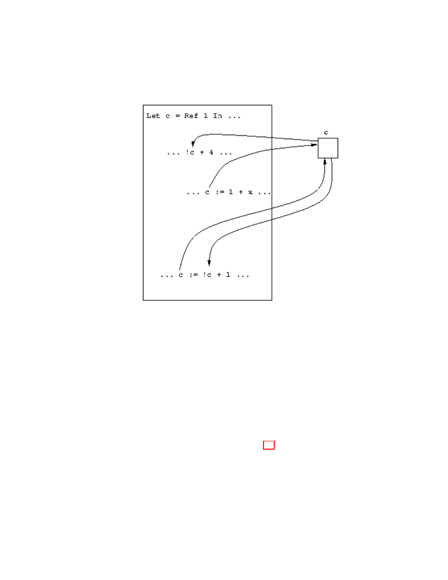
46
CHAPTER 4. SIDE EFFECTS: STATE AND EXCEPTIONS
Figure 4.1: The “junction box” view of reference cells.
examine the entire body of code to see which side-effects influence the outcome
of which expressions. Therefore, is it a good programming moral to use side-
effects sparingly, and only when needed.
Let us begin by informally discussing the semantics of references. In essence,
when a reference is created in a program, a cell is created that contains the
specified value, and the reference itself is a pointer to that cell. A good metaphor
for these reference cells is to think of each one as a junction box. Then, each
assignment is a path into the junction, and each read, or dereference, is a path
going out of the junction. The reference cell, or junction, sits to the side of
the program, and allows distant parts of the program to communicate with one
another. This “distant communication” can be a useful programming paradigm,
but again it should be used sparingly. Figure 4.1 illustrates this metaphor.
In the world of C
++
and Java, non-const (or non-final) global variables are
the most notorious form of reference. While globals make it easy to do certain
tasks, they generally make programs difficult to debug, since they can be altered
anywhere in the code.

4.1. STATE
47
4.1.1
The F[S Language
Adding state to our language involves making significant modifications to the
pure-functional languages that we’ve looked at so far. Therefore, we will spend a
bit of time developing a solid operational semantics for our state-based language
before looking at the interpreter. We will define a language F[S: F[ with state.
The most significant departure from the pure-functional operational seman-
tics we have looked at so far is that the evaluation relation e ⇒ v is not sufficient
to capture the semantics of a state-based language. The evaluation of an ex-
pression can now produce side-effects, and our ⇒ rule needs to incorporate this
somehow. Specifically, we will need to have someplace to record all these side-
effects: a store. In C, a store is a stack and a heap, and memory locations are
referenced by their addresses. When we are writing our interpreter, we will only
have access to the heap, so we will need to create an abstract store in which to
record side-effects.
Definition 4.1 (Store). A store is a finite map c 7→ v of cell names to values.
Cell names are an abstract representation of a memory location. A store is
therefore an abstraction of a runtime heap. The C heap is a low-level realization
of a store where the cell names are simply numerical memory addresses. A store
is also known as a dictionary from a data-structures perspective. We write
Dom(S) to refer the domain of this finite map, that is, the set of all cells that
it maps.
Let us begin by extending the concrete syntax of F[ to include F[S expres-
sions. The additions are as follows.
• Referencing, Ref e.
• Assignment, e := e
0
.
• Dereferencing, !e.
• Cell names, c.
We need cell names because Ref 5 needs to evaluate to a location, c, in the
store. Because cell names refer to locations in the heap, and the heap is initially
empty, programs have no cell names when the begin execution.
Although not part of the F[S syntax, we will need a notation to represent
operations on the store. We write S{c 7→ v} to indicate the store S extended
or modified to contain the mapping c 7→ v. We write S(c) to denote the value
of cell c in store S.
Now that we have developed the notion of a store, we can define a satisfactory
evaluation relation for F[S. Evaluation is written as follows.
he, S
0
i ⇒ hv, Si,

48
CHAPTER 4. SIDE EFFECTS: STATE AND EXCEPTIONS
where at the start of computation, S
0
is initially empty, and where S is the
final store when computation terminates. In the process of evaluation, cells, c,
will begin to appear in the program syntax, as references to memory locations.
Cells are values since they do not need to be evaluated, so the value space of
F[S also includes cells, c.
Evaluation Rules for F[S
Finally, we are ready to write the evaluation rules for F[S. We will need to
modify all of the F[ rules with the store in mind (recall that our evaluation
rule is now he, S
0
i ⇒ hv, Si, not simply e ⇒ v). We do this by threading
the store along the flow of control. Doing this introduces a great deal more
dependency between the rules, even the ones that do not directly manipulate
the store. We will rewrite the function application rule for F[S to illustrate the
types of changes that are needed in the other rules.
(Function Application)
he, S
1
i ⇒ hFunction x -> e, S
2
i, he
2
, S
2
i ⇒ hv
2
, S
3
i, he[v
2
/x], S
3
i ⇒ hv, S
4
i
he
1
e
2
, S
1
i ⇒ hv, S
4
i
Note how the store here is threaded through the different evaluations, showing
how changes in the store in one place propagate to the store in other places,
and in a fixed order that reflects the indented evaluation order. The rules for
our new memory operations are as follows.
(Reference Creation)
he, S
1
i ⇒ hv, S
2
i
hRef e, S
1
i ⇒ hc, S
2
{c 7→ v}i, for c /
∈ Dom(S
2
)
(Dereference)
he, S
1
i ⇒ hc, S
2
i
h!e, S
1
i ⇒ hv, S
2
i, where S
2
(c) = v
(Assignment)
he
1
, S
1
i ⇒ hc, S
2
i, he
2
, S
2
i ⇒ hv, S
3
i
he
1
:= e
2
, S
1
i ⇒ hv, S
3
{c 7→ v}i
These rules can be tricky to evaluate because the store needs to be kept up
to date at all points in the evaluation. Let us look at a few example expressions
to get a feel for how this works.

4.1. STATE
49
Example 4.1.
!(!(Ref Ref 5)) + 4
h!(!(Ref Ref 5)) + 4i, {}i ⇒ h9, {c
1
7→ 5, c
2
7→ c
1
}i, because
h!(!(Ref Ref 5)), {}i ⇒ h5, {c
1
7→ 5, c
2
7→ c
1
}i, because
h!(Ref Ref 5), {}i ⇒ hc
1
, {c
1
7→ 5, c
2
7→ c
1
}i, because
hRef Ref 5, {}i ⇒ hc
2
, {c
1
7→ 5, c
2
7→ c
1
}i, because
hRef 5, {}i ⇒ hc
1
, {c
1
7→ 5}i
Example 4.2.
(Function y -> If !y = 0 Then y Else 0) Ref 7
h(Function y -> . . . ) Ref 7, {}i ⇒ h0, {c
1
7→ 7}i, because
hRef 7, {}i ⇒ hc
1
, {c
1
7→ 7}i, and
h(If !y = 0 Then y Else 0)[c
1
/y], {c
1
7→ 7}i ⇒
h0, {c
1
7→ 7}i, because
h!c
1
= 0, {c
1
7→ 7}i ⇒ hFalse, {c
1
7→ 7}i, because
h!c
1
, {c
1
7→ 7}i ⇒ h7, {c
1
7→ 7}i
F[S Interpreters
Just as we had to modify the evaluation relation in our F[S operational seman-
tics to support state, writing a F[S interpreter will also require some additional
work. There are two obvious approaches to take, and we will treat them both
below. The first approach involves mimicking the operational semantics and
defining evaluation on an expression and a store together. This approach yields
a functional interpreter in which eval(e, S
0
) for expression e and initial state
S
0
returns the tuple (v, S), where v is the resulting value and S is the final
state.
The second and more efficient design involves keeping track of state in a
global, mutable dictionary structure. This is generally how real implementations
work.
This approach results in more familiar evaluation semantics, namely
eval e returns v. Obviously such an interpreter is no longer functional, but
rather, imperative. We would like such an interpreter to faithfully implement
the operational semantics of F[S, and thus we would ideally want a theorem
that states that this approach is equivalent to the first approach. Proving such
a theorem would be difficult, however, mainly because our proof would rely
on the operational semantics of Caml, or whatever implementation language

50
CHAPTER 4. SIDE EFFECTS: STATE AND EXCEPTIONS
we chose. We will therefore take it on good faith that the two approaches are
indeed equivalent.
The Functional Interpreter
The functional interpreter implements a state-
ful language in a functional way. It threads the state through the evaluation,
just as we did when we defined our operational semantics. Imperative style
programming can be “hacked” into a functional style by threading the state
along, and there are regular methods for threading state through any functional
programs, namely monads. The threading approach to modeling state func-
tionally was first employed by Strachey in the late 1960’s [22]. Note that an
operational semantics is always pure functional, since mathematics is always
purely functional.
To implement the functional interpreter, we model the store using a finite
mapping of integer keys to values. The skeleton of the implementation is pre-
sented below.
(* Declare all the expr, etc types globally for convenience. *)
(* The store functionality is a separate module.
*)
module type STORE =
sig
(* ... *)
end
(* The Store structure implements a (functional) store.
A simple
* implementation could be via a list of pairs such as
*
*
[((Cell 2),(Int 4)); ((Cell 3),Plus((Int 5),(Int 4))); ... ]
*)
module Store : STORE =
type store = (* ... *)
struct
let empty = (* initial empty store *)
let fresh = (* returns a fresh Cell name *)
let count = ref 0 in
function () -> ( count := !count + 1; Cell(!count) )
(* Note: this is not purely functional!
It is quite
* difficult to make fresh purely functional.
*)
(* Look up value of cell c in store s *)
let lookup (s,c) = (* ... *)

4.1. STATE
51
(* Add or modify cell c to point to value v in the store s.
* Return the new store.
*)
let modify(s,c,v) =
(* ... *)
end
(* The evaluator is then a functor taking a store module *)
module DSEvalFunctor =
functor (Store : STORE) ->
struct
(* ... *)
let eval (e,s) = match e with
(Int n) -> ((Int n),s) (* values don’t modify store *)
| Plus(e,e’) ->
let (Int n,s’) = eval(e,s) in
let (Int n’,s’’) = eval(e’,s’) in
(Int (n+n’),s’’)
(* Other cases such as application use a similar store
* threading technique.
*)
| Ref(e) -> let (v,s’) = eval(e,s) in
let c = Store.fresh() in
(c,Store.modify(s’,c,v))
| Get(e) -> let (Cell(n),s’) = eval(e,s) in
(Store.lookup(Cell(n)),s)
| Set(e,e’) ->
(* exercise *)
end
module DSEval = DSEvalFunctor(Store)
The Imperative Interpreter
The stateful, imperative F[S interpreter is
more efficient than its functional counterpart, because no threading is needed.
In the imperative interpreter, we represent the store as a dictionary structure
(similar to Java’s HashMap class or the C
++
STL map template). The eval
function needs no extra store parameter, provided that it has a reference to
the global dictionary. Non-store-related rules such as Plus and Minus are com-
pletely ignorant of the store. Only the direct store evaluation rules, Ref, Set,
and Get actually extend, update, or query the store. A good evaluator would
52
CHAPTER 4. SIDE EFFECTS: STATE AND EXCEPTIONS
Figure 4.2: A simple cycle.
also periodically garbage collect, or remove unneeded store elements. Garbage
collection is discussed briefly in Section 4.1.4. The implementation of the state-
ful interpreter is left as an exercise to the reader.
Side-Effecting Operators
Now that we have a mutable store, our code has properties beyond the value
that is returned, namely, side-effects. Operators such as sequencing (;), and
While- and For loops now become relevant. These syntactic concepts are easily
defined as macros, so we will not add them to the official F[S syntax. The
macro definitions are as follows.
e
1
; e
2
= (Function x -> e
2
) e
1
While e Do e
0
= Let Rec f x = If e Then f e
0
Else 0 In f 0
Exercise 4.1. Why are sequencing and loop operations irrelevant in pure func-
tional languages like F[?
4.1.2
Cyclical Stores
An interesting phenomenon is possible with stateful languages. It is possible
to make a cyclical store, that is, a cell whose contents are a pointer to itself.
Creating a cyclic store is quite easy:
Let x = Ref 0 in x := x
This is the simplest possible store cycle, where a cell directly points to itself.
This type of store is illustrated in Figure 4.2.
Exercise 4.2. In the above example, what does !!!!!!!!x return? Can a store
cycle like the one above be written in Caml? Why or why not? (Hint: What is
the type of such an expression?)

4.1. STATE
53
A more subtle form of a store cycle is when a function is placed in the cell,
and the body of the function refers to that cell. Consider the following example.
Let c = Ref 0 In
c := (Function x -> If x = 0 Then 0 Else 1 + !c(x-1));
!c(10)
Cell c contains a function, which, in turn, refers to c. In other words, the
function has a reference to itself, and can apply itself, giving us recursion. This
form of recursion is known as tying the knot, and is the method used by
most compilers to implement recursion. A similar technique is used to make
objects self-aware, although C
++
explicitly passes self, and is more like the Y -
combinator.
Exercise 4.3. Tying the knot be written in Caml, but not directly as above.
How must the reference be declared for this to work? Why can we create this
sort of cyclic store, but not the sort described in Exercise 4.2?
Interact with F[SR. Let’s write a recursive multiplication function in
F[SR, first using Let Rec, and then by tying the knot.
# Let Rec mult x = Function y ->
If x = 0 Then
0
Else
y + mult (x - 1) y In
mult 8 9;;
==> 72
Now we’ll use tying the knot. Because F[SR does not include a sequencing
operation, we use the encoding presented in Section 4.1.1.
# Let mult = Ref 0 In
(Function dummy -> (!mult) 9 8)
(mult := (Function x -> Function y ->
If x = 0 Then
0
Else
y + (!mult) (x - 1) y));;
==> 72

54
CHAPTER 4. SIDE EFFECTS: STATE AND EXCEPTIONS
4.1.3
The “Normal” Kind of State
Languages like C
++
, Java, and Scheme have a different form for expressing
mutation. There is no need for an explicit dereference (!) operator to get
the value of a cell. This form of mutation is more difficult to capture in an
interpreter, because variables mean something different depending on whether
they are on the left or right side of an assignment operator. An l-value occurs
on the left side of the assignment, and represents a memory location. An r-
value to the right of an assignment, or elsewhere in the code, and represents
an actual value.
Consider the C/C
++
/Java assignment statement x = x + 1. The x on the
left of the assignment is an l-value, and the x in x + 1 is an r-value. In Caml,
we would write a similar expression as x := !x + 1. Thus, Caml is explicit in
which is being referred to, the cell or the value. For a Java l-value, the cell is
needed to perform the store operation, and for a Java r-value, the value of the
cell is needed, which is why, in Caml, we must write !x.
l-values and r-values are distinct. Some expressions may be both l-values
and r-values, such as x and x[3]. Other values may only be r-values, such as
5, (0 == 1), and sin(3.14159). Therefore, l-values and r-values are expressed
differently in the language grammar, specifically, l-values are a subset of r-values.
There are some shortcomings to such languages. For example, in Caml we can
say f(3) := 1, which assigns the value 1 to the cell returned by the function f.
Expressions of this sort are invalid in Java, because f(3) is not an l-value. We
could revise the F[S grammar to use this more restrictive notion, where l-values
must only be variables, in the following way:
type expr =
...
| Get of expr | Set of ident * expr | Ref of expr
For the variable on the left side of the assignment, we would need the address,
and not the contents, of the variable.
A final issue with the standard notion of state in C and C
++
is the problem
of uninitialized variables. Because variables are not required to be initialized,
runtime errors due to these uninitialized variables are possible. Note that the
Ref syntax of F[S and Caml requires that the variable be explicitly initialized
as part of its declaration.
4.1.4
Automatic Garbage Collection
Memory that is allocated may also, at some point, be freed. In C and C
++
, this
is done explicitly with free() and delete() respectively. However, Java, Caml,
Smalltalk, Scheme, and Lisp, to name a few, support the automated freeing of
unused memory through a garbage collector.
Garbage collection is a large area of research (see [23] for a survey), but we
will briefly sketch out what an implementation looks like.

4.2. ENVIRONMENT-BASED INTERPRETERS
55
First, something triggers the garbage collector. Generally, the trigger is that
the store is getting too full. In Java, the garbage collector may be explicitly
invoked by the method System.gc(). When the garbage collector is invoked,
evaluation is suspended until the garbage collector has completed. The garbage
collector proceeds to scan through the current computation to find cells that
are directly used. The set of these cells is known as the root set. Good places
to look for roots are on the evaluation stack and in global variable locations.
Once the root set is established, the garbage collector marks all cells not in
the root set as initially free. Then, it recursively traverses the memory graph
starting at the root set, and marks cells that are reachable from the root set
as not free, thus at the end of the traversal, all cells that are in a different
connected component from any of the cells in the root set are marked not free,
and these cells may be reused. There are many different ways to reuse memory,
but we will not go into detail here.
4.2
Environment-Based Interpreters
Now that we have discussed stateful languages, we are going to briefly touch on
some efficiency issues with the way we have been defining interpreters. We will
focus on eliminating explicit substitutions in function application.
A “low-level” interpreter would never duplicate the function argument for
each variable usage. The problem with doing so is that it can severely increase
the size of the data that must be maintained by the interpreter. Consider an
expression in the following form.
(Function x -> x x x) (whopping expr)
This expression is evaluated by computing
(whopping expr)(whopping expr)(whopping expr),
tripling the size of the data.
In order to solve this problem, we define an explicit environment inter-
preter. In an explicit environment interpreter, instead of doing direct variable
substitution, we keep track of each variable’s value in a runtime environment.
The runtime environment is simply a mapping of variables to values. We write
environments as {x
1
7→ v
1
, x
2
7→ v
2
}, to mean that variable x
1
maps to value
v
1
and variable x
2
maps to value v
2
.
Now, to compute
(Function x -> x x x)(whopping expr)

56
CHAPTER 4. SIDE EFFECTS: STATE AND EXCEPTIONS
the interpreter computes (x x x) in the environment {x 7→ whopping expr}.
Technically, even the simple substituting interpreters we’ve looked at don’t
really make three copies of the data. Rather, they maintain a single copy of
the data and three pointers to it. This is because immutable data can always
be passed by reference since it never changes. However, in a compiler the code
can’t be copied around like this, so a scheme like the one presented above is
necessary.
There is a possibility for some anomalies with this approach, however. Specif-
ically, there is a problem when a function is returned as the result of another
function application, and the returned function has local variables in it. Con-
sider the following example.
f = Function x -> If x = 0 Then
Function y -> y
Else Function y -> x + y
When f (3) is computed, the environment binds x to 3 while the body is
computed, so the result returned is
Function y -> x + y,
but it would be a mistake to simply return this as the correct value, because we
would lose the fact that x was bound to 3. The solution is that when a function
value is returned, the closure of that function is returned.
Definition 4.2 (Closure). A closure is a function along with an environ-
ment, such that all free values in the function body are bound to values in the
environment.
For the case above, the correct value to return is the closure
(Function y -> x + y, {x 7→ 3})
Theorem 4.1. A substitution-based interpreter and an explicit environment
interpreter for F[ are equivalent: all F[ programs either terminate on both in-
terpreters or compute forever on both interpreters.
This closure view of function values is critical when writing a compiler, since
compiler’s should not be doing substitutions of code on the fly. Compilers are
discussed in Chapter 7.
4.3. THE F[SR LANGUAGE
57
4.3
The F[SR Language
We can now define the F[SR language. F[SR is the call-by-value language that
included the basic features of F[, and is extended to include records (F[R), and
state (F[S).
In Section 4.4 and Chapters 5 and 6, we will study the language features
missing from F[SR, namely objects, exceptions, and types. In Chapter 7, we
will discuss translations for F[SR, but will not include these other language
features. The abstract syntax type for F[SR is as follows.
type label = Lab of string
type ident = Ident of string
type expr =
Var of ident | Function of ident * expr | Appl of expr * expr |
Letrec of ident * ident * expr * expr | Plus of expr * expr |
Minus of expr * expr | Equal of expr * expr |
And of expr * expr | Or of expr * expr | Not of expr |
If of expr * expr * expr | Int of int | Bool of bool |
Ref of expr | Set of expr * expr | Get of expr | Cell of int |
Record of (label * expr) list | Select of
label * expr |
Let of ident * expr * expr
In the next two sections we will look at some nontrivial “real-world” F[SR
programs to illustrate the power we can get from this simple language. We
begin by considering a function to calculate the factorial function, and conclude
the chapter by examining an implementation of the merge sort algorithm.
4.3.1
Multiplication and Factorial
The factorial function is fairly easy to represent using F[SR. The main point of
interest here is the encoding of multiplication using a curried Let Rec definition.
This example assumes a positive integer input.
(*
* First we encode multiplication for positive nonnegative
* integers.
Notice the currying in the Let Rec construct.
* Multiplication is encoded in the obvious way: repeated
* addition.
*)
Let Rec mult x = Function y ->
If y = 0 Then
0
Else
x + (mult x (y - 1)) In

58
CHAPTER 4. SIDE EFFECTS: STATE AND EXCEPTIONS
(*
* Now that we have multiplication, factorial is easy to
* define.
*)
Let Rec fact x =
If x = 0 Then
1
Else
mult x (fact (x - 1)) In
fact 7
4.3.2
Merge Sort
Writing a merge sort in F[SR is a fairly comprehensive example. One of the
biggest challenges is encoding integer comparisons, i.e. <, >, etc. Let’s discuss
how this is accomplished before looking at the code.
First of all, given that we already have an equality test, =, encoding the <=
operation basically gives us the other standard comparison operations for free.
Assuming that we have a lesseq function, the other operations can be trivially
encoded as follows.
Let lesseq = (* real definition *) In
Let lessthan = (Function x -> Function y ->
(lesseq x y) And Not (x = y)) In
Let greaterthan = (Function x -> Function y ->
Not (lesseq x y)) In
Let greatereq = (Function x -> Function y ->
(greaterthan x y) Or (x = y)) In ...
Therefore it suffices to encode lesseq. But how can we do this using only
the regular F[SR operators? The basic idea is as follows. To test if x is less
than or equal to y we compute a z such that x + z = y. If z is nonnegative,
we know that x is less than or equal to y. If z is negative, we know that x is
greater than y.
At first glance, we seem to have a “chicken and egg” problem here. How
can we tell if z is negative if we have no comparison operator. And how do we
actually compute z to begin with? One idea would be to start with z = 0 and
loop, incrementing z by 1 at every step, and it testing if x + z = y. If we find
a z, we stop. We know that z is positive, and we conclude that x is less than
or equal to y. If we don’t find a z, we start at z = −1 and perform a similar
loop, decrementing z by 1 every step. If we find a proper value of z this way,
we conclude that x is greater then y.

4.3. THE F[SR LANGUAGE
59
The flaw in the above scheme should be obvious: if x > y, the first loop
will never terminate. Indeed we would need to run both loops in parallel for
this idea to work! Obviously F[SR doesn’t allow for parallel computation, but
there is a solution along these lines. We can interleave the values of z that are
tested by the two loops. That is, we can try the values {0, −1, 1, −2, 2, −3, . . .}.
The great thing about this approach is that every other value of z is negative,
and we can simply pass along a boolean value to represent the sign of z. If z
is nonnegative, the next iteration of the loop inverts it and subtracts 1. If z is
negative, the next iteration simply inverts it. Note that we can invert the sign
of an number x in F[SR by simply writing 0 - x. Now, armed with our ideas
about lesseq, let us start writing our merge sort.
(* We need to represent the empty list somehow.
Since we
* will need to test for it, and since equality is only
* defined on integers, emptylist will need to be an
* integer.
We define it as -1.
*)
Let emptylist = (0 - 1) In
(* Next, let’s define some list operations, head, tail,
* cons, and length.
There encodings are straightforward,
* and were covered in the text.
Notice that we are
* encoding lists as records, using {l,r} records like
* pairs.
*)
Let head = Function seq -> seq.l In
Let tail = Function seq -> seq.r In
Let cons = Function elt -> Function seq -> {l=elt; r=seq} In
Let Rec length seq =
If seq = emptylist Then
0
Else
1 + length (seq.r) In
(* Now, we’re ready to define lesseq.
Notice how lesseq is
* a wrapper function that uses le.
le passes along the
* sign of v as an argument, as discussed in the text.
*)
Let lesseq = Function a -> Function b ->
Let Rec le x =
Function y -> Function v ->

60
CHAPTER 4. SIDE EFFECTS: STATE AND EXCEPTIONS
Function v is non neg ->
If (x + v) = y Then
v is non neg
Else
If v is non neg Then
le x y (0 - v - 1) (Not v is non neg)
Else
le x y (0 - v) (Not v is non neg) In
le a b 0 True In
(* This function takes a list and splits it into nearly
* equal halves.
These halves are returned as a pair
* (encoded as an {left, right} record).
*)
Let split = Function seq ->
Let Rec splt seq1 = Function seq2 ->
If lesseq (length seq1) (length seq2) Then
{left=seq1; right=seq2}
Else
splt (tail seq1) (cons (head seq1) seq2) In
splt seq emptylist In
(* Here is where we merge two sorted lists.
We scan through
* each list in parallel, chopping off the smaller of the
* two list heads and appending it to the result.
This is
* where we make use of our lesseq function.
*)
Let Rec merge seq1 = Function seq2 ->
If seq1 = emptylist Then
seq2
Else If seq2 = emptylist Then
seq1
Else
If lesseq (head seq1) (head seq2) Then
cons (head seq1) (merge (tail seq1) seq2)
Else
cons (head seq2) (merge seq1 (tail seq2)) In
(* mergesort sorts a single list by breaking it into two
* smaller lists, recursively sorting those lists, and
* merging the two back into a single list.
Recall that
* the base cases of the recursion are a single element list
* and an empty list, both of which are necessarily in
* sorted order by definition.
*)
Let Rec mergesort seq =

4.4. EXCEPTIONS AND OTHER CONTROL OPERATIONS
61
If lesseq (length seq) 1 Then
seq
Else
Let halves = split seq In
merge (mergesort (halves.left))
(mergesort (halves.right)) In
(* Finally we call mergesort on an actual list.
Notice the
* record encoding.
*)
mergesort {l=5;
r=
{l=6;
r=
{l=2;
r=
{l=1;
r=
{l=4;
r=
{l=7;
r=
{l=8;
r=
{l=10; r=
{l=9;
r=
{l=3;
r=emptylist}}}}}}}}}}
4.4
Exceptions and Other Control Operations
Until now, expressions have been evaluated by marching through the evaluation
rules one at a time. To perform addition, the left and right operands were
evaluated to values, after which the addition expression itself was evaluated to
a value. This addition expression may have been part of a larger expression,
which could then itself have been evaluated to a value, etc.
In this section, we will discuss explicit control operations, concentrating
on exceptions. Explicit control operations are operations that explicitly alter
the control of the evaluation process. Even simple languages have control oper-
ations. A common example is the return statement in C
++
and Java.
In F[, the value of the function is whatever its entire body evaluates to.
If, in the middle of some complex conditional loop expression, we have the
final result of the computation, it is still necessary to complete the execution
of the function. A return statement gets around this problem by immediately
returning from the function and aborting the rest of the function computation.
Another common control operation is the loop exit operation, or break in
C
++
or Java. break is similar to return, except that it exits the current loop
instead of the entire function.
These types of control operations are interesting, but in this section, we will
concentrate more on two more powerful control operations, namely exceptions

62
CHAPTER 4. SIDE EFFECTS: STATE AND EXCEPTIONS
and exception handlers. The reader should already be familiar with the basics
of exceptions from working with the Caml exception mechanism.
There are some other control operations that we will not discuss, such as
the call/cc, shift/reset, and control/prompt operators.
We will avoid the goto operator in this section, except for the following brief
discussion. goto basically jumps to a labeled position in a function. The main
problem with goto is that it is too raw. The paradigm of jumping around be-
tween labels is not all that useful in the context of functions. It is also inherently
dangerous, as one may inadvertently jump into the middle of a function that
is not even executing, or skip past variable initializations. In addition, with a
rich enough set of other control operators, goto really doesn’t provide any more
expressiveness, at least not meaningful expressiveness.
The truth is that control operators are really not needed at all.
Recall
that F[, and the lambda calculus for that matter, are already Turing-complete.
Control operators are therefore just conveniences that make programming easier.
It is useful to think of control operators as “meta-operators,” that is, operators
that act on the evaluation process itself.
4.4.1
Interpreting Return
How are exceptions interpreted? Before we answer this question, we will consider
adding a Return operator to F[, since it is a simpler control operator than
exceptions. The trouble with Return, and with other control operators, is that
it doesn’t fit into the normal evaluation scheme. For example, consider the
expression
(Function x ->
(If x = 0 Then 5 Else Return (4 + x)) - 8) 4
Since x will not be 0 when the function is applied, the Return statement will
get evaluated, and execution should stop immediately, not evaluating the “-
8.” The problem is that evaluating the above statement means evaluating
(If 4 = 0 Then 5 Else Return (4 + 4)) - 8,
which, in turn, means evaluating
(Return (4 + 4)) - 8.
But we know that the subtraction rule works by evaluating the left and right
hand sides of this expression to values, and performing integer subtraction on

4.4. EXCEPTIONS AND OTHER CONTROL OPERATIONS
63
them. Clearly that doesn’t work in this case, and so we need a special rules for
subtraction with a Return in one of the subexpressions.
First, we need to add Returns to the value space of F[ and provide an
appropriate evaluation rule:
(Return)
e ⇒ v
Return e ⇒ Return v
Next, we need the special subtraction rules, one for when the Return is on the
left side, and one for when the Return is on the right side.
(- Return Left)
e ⇒ Return v
e - e
0
⇒ Return v
(- Return Right)
e ⇒ v, e
0
⇒ Return v
0
e - e
0
⇒ Return v
0
Notice that these subtraction rules evaluate to Return v and not simply v.
This means that the Return is “bubbled up” through the subtraction operator.
We need to define similar return rules for every F[ operator. Using these new
rules, it is clear that
Return (4 + 4) - 8 ⇒ Return 8.
Of course, we don’t want the Return to bubble up indefinitely. When the
Return pops out of the function application, we only get the value associated
with it. In other words, our original expression,
(Function x ->
(If x = 0 Then 5 Else Return (4 + x)) - 8) 4
should evaluate to 8, not Return 8. To accomplish this, we need a special
function application rule.
(Appl. Return)
e
1
⇒ Function x -> e, e
2
⇒ v
2
, e[v
2
/x] ⇒ Return v
e
1
e
2
⇒ v
A few other special application rules are needed for the cases when either the
function or the argument itself is a Return.

64
CHAPTER 4. SIDE EFFECTS: STATE AND EXCEPTIONS
(Appl. Return Function)
e
1
⇒ Return v
e
1
e
2
⇒ Return v
(Appl. Return Arg.)
e
1
⇒ v
1
, e
2
⇒ Return v
e
1
e
2
⇒ Return v
Of course, we still need the original function application rule (see Section 2.3.3)
for the case that function execution implicitly returns a value by dropping off
the end of its execution.
Let us conclude our discussion of Return by considering the effect of Return
Return e. There are two possible interpretations for such an expression. By the
above rules, this expression returns from two levels of function calls. Another
interpretation would be to add the following rule:
(Double Return)
e ⇒ Return v
Return e ⇒ Return v
Of course we would need to restrict the original Return rule to the case where
v was not in the form Return v. With this rule, instead of returning from
two levels of function calls, the second Return actually interrupts and bubbles
through the first. Of course, double returns are not a common construct, and
these rules will not be used often in practice.
4.4.2
The F[X Language
The translation of Return that was given above can easily be extended to
deal with general exceptions. We will define a language F[X, which is F[ ex-
tended with a Caml-style exception mechanism. F[X does not have Return
(nor does Caml), but Return is easily encodable with exceptions. For example,
the “pseudo-Caml” expression
(function x -> (if x = 0 then 5 else return (4 + x)) - 8) 4
can be encoded in the following manner.
exception Return of int;;
(function x ->
try
(if x = 0 then 5 else raise (Return (4 + x))) - 8
with
Return n -> n) 4;;

4.4. EXCEPTIONS AND OTHER CONTROL OPERATIONS
65
Return can be encoded in other functions in a similar manner.
Now, let’s define our F[X language. The basic idea is very similar to the
Return semantics that we discussed above. We define a new kind of value,
Raise xn,
which bubbles up the exception xn. This is the generalization of the value class
Return v from above. xn is a metavariable representing an exception. An ex-
ception contains two pieces of data: a name, and an argument. The argument
can be any arbitrary expression. Although we only allow single-argument excep-
tions, zero-valued or multi-valued versions of exceptions can be easily encoded
by, for example, supplying the exception with a record argument with zero, one,
or several fields. We also add to F[X the expression
Try e With name arg -> e
0
Note that Try binds free values of arg in e
0
. The metavariable name is the
name of an exception to be caught, and not an actual exception expression.
Also notice that the F[X Try syntax differs slightly from the Caml syntax in
that Caml allows an arbitaray pattern-match expression in the With clause. We
allow only a single clause that matches all values of arg.
F[X is untyped, so exceptions do not need to be declared. We use the “#”
symbol to designate exceptions in the concrete syntax, for example, #MyExn.
Below is an example of a F[X expression.
Function x -> Try
(If x = 0 Then 5 Else Raise (#Return (4 + x))) - 8
With #Return n -> n) 4
Exceptions are side-effects, and can cause “action at a distance.” Therefore,
like any other side-effects, they should be used sparingly.
4.4.3
Implementing the F[X Interpreter
The abstract syntax type for F[X is as follows.
type expr =
...
| Raise of expr
| Try of expr * string * ident * expr
| Exn of string * expr

66
CHAPTER 4. SIDE EFFECTS: STATE AND EXCEPTIONS
The rules for Raise and Try are derived from the return rule and the ap-
plication return rule respectively. Raise “bubbles up” an exception, just like
Return bubbled itself up. Try is the point at which the bubbling stops, just like
function application was the point at which a Return stopped bubbling. The
operational semantics of exceptions are as follows.
(Exception)
e ⇒ v, for v not of the form Raise . . .
#xn e ⇒ #xn v
(Raise)
e ⇒ #xn v
Raise e ⇒ Raise (#xn v)
(Try)
e ⇒ v for v not of the form Raise (#xn v)
Try e With #xn x -> e
0
⇒ v
(Try Catch)
e ⇒ Raise (#xn v), e
0
[v/x] ⇒ v
0
Try e With #xn x -> e
0
⇒ v
0
In addition, we need to add special versions of all of the other F[ rules so
that the Raise bubbles up through the computation just as the Return did.
For example
(- Raise Left)
e ⇒ Raise (#xn v)
e - e
0
⇒ Raise (#xn v)
Note that we must handle the unusual case of when a Raise bubbles through a
Raise, something that will not happen very often in practice. The rule is very
much like the “- Raise Left” rule above.
(Raise Raise)
e ⇒ Raise (#xn v)
Raise e ⇒ Raise (#xn v)
Now, let’s trace through the execution of
Function x -> Try
(If x = 0 Then 5 Else Raise (#Return (4 + x))) - 8
With #Return n -> n) 4
After the function application and the evaluation of the If statement, we are
left with
Try (Raise (#Return(4 + 4))) - 8
With #Return n -> n

4.4. EXCEPTIONS AND OTHER CONTROL OPERATIONS
67
which is
Try Raise (#Return 8) - 8
With #Return n -> n
which by bubbling in the subtraction computes to
Try Raise (#Return 8)
With #Return n -> n
which by the Try Catch rule returns the value 8, as expected.
4.4.4
Efficient Implementation of Exceptions
The “bubbling up” method of interpretation is operationally correct, but in
practice is very inefficient. For instance, the subtraction rule will always have
to check if either argument is in Raise form before it decides how to act, which
greatly slows down the speed of the interpreter. It’s possible to write better
interpreters that address this problem, but for our purposes, we will only deal
with this problem in the context of compilers. Compilers are discussed at length
in Chapter 7, and so it may be wise to skip this section for now and return to
it after reading about compilers.

68
CHAPTER 4. SIDE EFFECTS: STATE AND EXCEPTIONS

Chapter 5
Object-Oriented Language
Features
Object-oriented programming can today be declared a success. Introductory
programming courses are often taught using object-oriented languages such
as C
++
and Java.
Most new commercial projects choose an object-oriented
language. Yet, object-oriented features do not fundamentally add much to a
language.
They certainly do not lead to shorter programs.
The success of
object-oriented programming is due mainly to the fact that it is a style that is
appropriate for the human psychology. Humans, as part of their basic function,
are highly adept at recognizing and interacting with everyday objects. And,
objects in programming are enough like objects in the everyday world that our
rich intuitions can apply to them.
Before we discuss the properties of objects in object-oriented programming,
let us briefly review some of the more important properties of everyday objects
that would make them useful for programming.
• Everyday objects are active, that is, they are not fully controlled by us.
Objects have internal and evolving state. For instance, a running car is an
active object, and has a complex internal state including the amount of gas
remaining, the engine coolant and transmission fluid levels, the amount of
battery power, the oil level, the temperature, the degree of wear and tear
on the engine components, etc.
• Everyday objects are communicative. We can send messages to them, and
we can get feedback from objects as a result of sending them messages.
For example, starting a car and checking the gas gauge can both be viewed
as sending messages to the car.
1
It may, at first, seem unnatural to view checking the gas gauge as sending a message.
After all, it is really the car sending a message to us. We view ourselves as the “sender,”
however, because we initiated the check, that is, in a sense, we asked the car how much gas
was remaining.
69

70
CHAPTER 5. OBJECT-ORIENTED LANGUAGE FEATURES
• Everyday objects are encapsulated. They have internal properties that we
can not see, although we can learn some of them by sending messages. To
continue the car example, checking the gas gauge tells us how much gas
is remaining, even though we can’t see into the gas tank directly, and we
don’t know if it contains regular or premium gas.
• Everyday objects may be nested, that is, objects may be made up of several
smaller object components, and those components may themselves have
smaller components. Once again, a car is a perfect example of a nested
object, being made of of smaller objects including the engine and the
transmission. The transmission is also a nested object, including an input
shaft, an output shaft, a torque converter, and a set of gears.
• Everyday objects are, for the most part, uniquely named. Cars are uniquely
named by license places or vehicle registration numbers.
• Everyday objects may be self-aware, in the sense that they may intention-
ally interact with themselves, for instance a dog licking his paw.
• Everyday object interactions may be polymorphic in that a diverse set of
objects may share a common messaging protocol, for example the accel-
erator/brake/steering wheel messaging system common to all models of
cars and trucks.
The objects in object-oriented programming also have these properties. For
this reason, object-oriented programming has a natural and familiar feel to most
people. Let us now consider objects of the programming variety.
• Objects have an internal state in the form of instance variables or fields.
Objects are generally active, and their state is not fully controlled by their
callers.
• Objects support messages, which are named pieces of code that are tied
to a particular object. In this way objects are communicative, and groups
of objects accomplish tasks by sending messages to each other.
• Objects consist of encapsulated code (methods or operations) along with a
mutable state (instance variables or fields). Right away it should be clear
that objects are inherently non-functional. This mirrors the statefulness
of everyday objects.
• Objects are typically organized in a nested fashion. For example, consider
an object that represents a graphical web browser. The object itself is
frame, but that frame consists of a toolbar and a viewing area. The toolbar
is made up of buttons, a location bar, and a menu, while the viewing area
is made up of a rendered panel and a scroll bar. This concept is illustrated
in Figure 5.1. Object nesting is generally accomplished by the outer object
storing its inner objects as fields or instance variables.
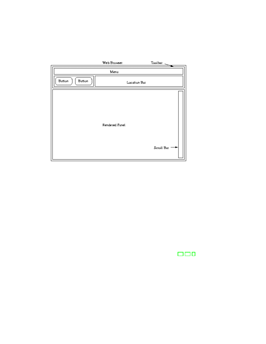
71
Figure 5.1: A nested object representing a web browser.
• Objects have unique names, or object references, to refer to them. This
is analogous to the naming of real-world objects, with the advantage that
object references are always unique whereas real-world object names may
be ambiguous.
• Objects are self aware, that is, objects contain references to themselves.
this in Java and self in Smalltalk are self-references.
• Objects are polymorphic, meaning that a “fatter” object can always be
passed to a method that takes a “thinner” one, that is, one with fewer
methods and public fields.
There are several additional features objects commonly have. Classes are
nearly always present in languages with objects. Classes are not required: it
is perfectly valid to have objects without classes. The language Self [19, 20, 1]
has no classes, instead it has prototype objects which are copied that do the
duty of classes. Important concepts of classes include creation, inheritance,
method overriding, superclass access, and dynamic dispatch. We will address
these concepts later.
Information hiding for fields and methods is another feature that most
object-oriented languages have, generally in the form of public, private, and
protected keywords.
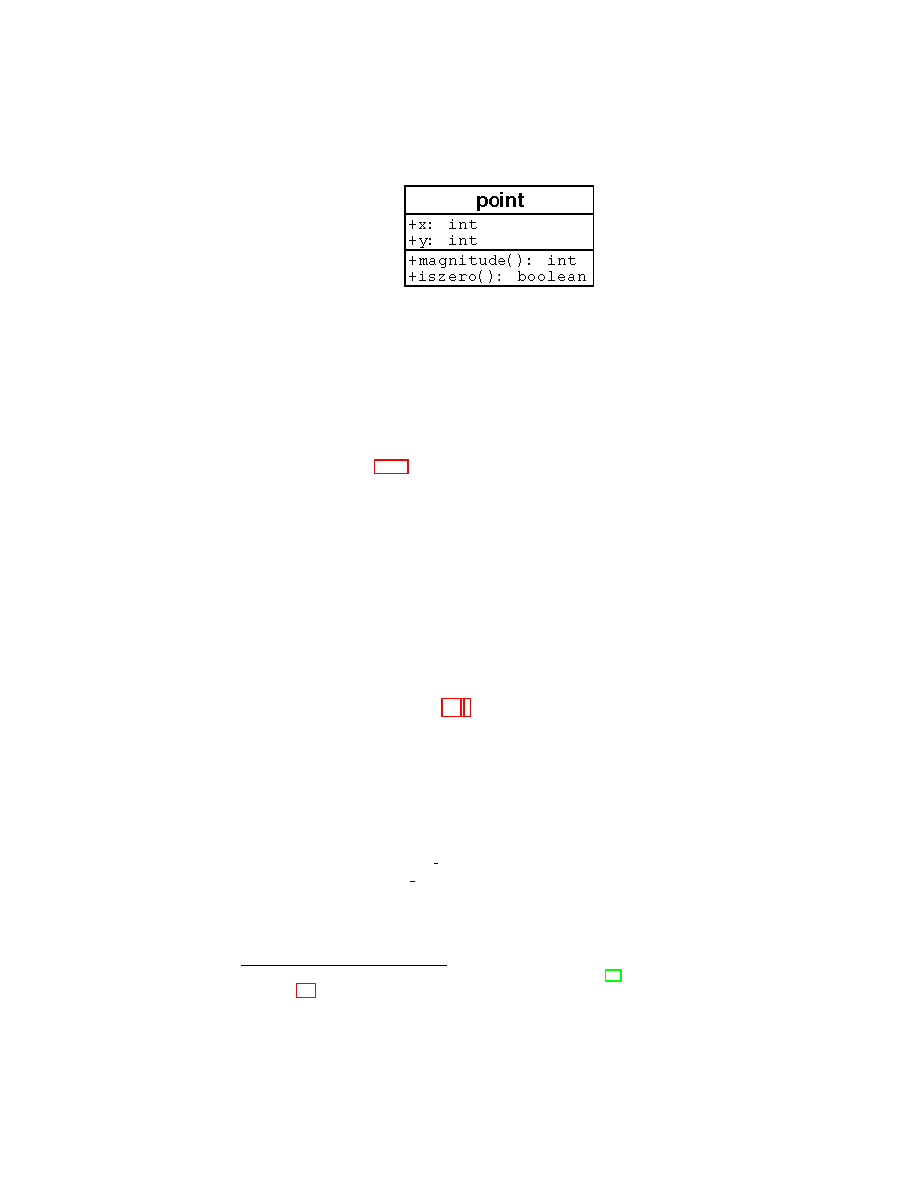
72
CHAPTER 5. OBJECT-ORIENTED LANGUAGE FEATURES
Figure 5.2: The “point” object.
Other aspects of objects include object types and modules. Types are dis-
cussed briefly, but modules are beyond the scope of this book. We also ignore
method overloading, as it is simply syntactic sugar and adds only to readabil-
ity, not functionality. Recall that overloading a method means there are two
methods with the same name, but different type signatures. Overriding means
redefining the behavior of a superclass’s method in a subclass. Overriding is
discussed in Section 5.1.5.
5.1
Encoding Objects in F[SR
One of the most important aspects of objects is how close they are to existing
concepts that we have already discussed. In this section we demonstrate how
objects may be encoded in F[SR. We will model objects as records of functions
and references. Record labels and values can be thought of as slots for either
methods or fields. A slot with a function is a method, and a slot with a reference
is a field.
5.1.1
Simple Objects
Consider the object in Figure 5.2
that represents a point in two-dimensional
space. The object has fields x and y, along with two methods: magnitude and
iszero, with obvious functionality. To encode this object as a record, we are
going to need a record that has the following structure.
Let point = {
x = 4;
y = 3;
magnitude = Function
-> . . . ;
iszero = Function
-> . . .
} In . . .
We can’t write the magnitude method yet, because we need to define it in
terms of x and y, but there is no way to refer to them in the function body. The
2
We use UML to diagram objects. UML is fully described in [10]. Although the diagram
in Figure 5.2 is technically a class diagram, for our purposes we will view it simply as the
induced object.

5.1. ENCODING OBJECTS IN F[SR
73
solution we will use is the same one that C
++
uses behind the scenes: we pass
the object itself as an argument to the function. Let’s revise our first encoding
to the following one (assuming we’ve defined a sqrt function).
Let point = {
x = 4;
y = 3;
magnitude = Function this -> Function
->
sqrt this.x + this.y;
iszero = Function this -> Function
->
(this.magnitude this {}) = 0
} In . . .
There are a few points of interest about the above example. First of all,
the object itself needs to be explicitly passed as an argument when we send
a message. For example, to send the magnitude message to point, we would
write
point.magnitude point {}.
For convenience, we can use the abbreviation obj <- method to represent the
message (obj.method obj).
Even inside the object’s methods, we need to pass this along when we call
another method. iszero illustrates this point in the way it calls magnitude.
This encoding of self-reference is called the self-application encoding. There
are a number of other encodings, and we will treat some of them below.
There is a problem with this encoding, though; our object is still immutable.
An object with immutable fields can be a good thing in many cases. For ex-
ample, windows that can’t be resized and sets with fixed members can be im-
plemented with immutable fields. In general, though, we need our objects to
support mutable fields. Luckily this problem has an easy solution. Consider the
following revision of our point encoding, which uses Refs to represent fields.
Let point = {
x = Ref 4;
y = Ref 3;
magnitude = Function this -> Function
->
sqrt !(this.x) + !(this.y);
iszero = Function this -> Function
->
(this.magnitude this {}) = 0
setx = Function this -> Function newx -> this.x := newx
sety = Function this -> Function newy -> this.y := newy
} In . . .

74
CHAPTER 5. OBJECT-ORIENTED LANGUAGE FEATURES
To set x to 12, we can write either point <- setx 12, or we can directly
change the field with (point.x) := 12. To access the field, we now write
!(point.x), or we could define a getx method to abstract the dereferencing.
This strategy gives us a faithful encoding of simple objects. In the next few
sections, we will discuss how to encode some of the more advanced features of
objects.
5.1.2
Object Polymorphism
Suppose we define the following function.
Let tallerThan = Function person1 -> Function person2 ->
greatereq (person1 <- height) (person2 <- height)
If we were to define person objects that supported the height message, we
could pass them as arguments to this function. However, we could also create
specialized person objects, such as mother, father, and child. As long as
these objects still support the height message, they are all valid candidates
for the tallerThan function. Even objects like dinosaurs and buildings can
be arguments. The only requirement is that any objects passed to tallerThan
support the message height. This is known as object polymorphism.
We already encountered a similar concept when we discussed record poly-
morphism. Recall that a function
Let getheight = Function r -> r.height . . .
can take any record with a height field:
. . . In getheight {radius = 4; height = 4; weight = 44}
Object polymorphism is really the same as record polymorphism, evidenced
by how we view objects as records. So simply by using the record encoding of
objects, we can easily get object polymorphism.
Let eqpoint = {
(* all the code from point above: x, y, magnitude . . . *)
equal = Function this -> Function apoint ->
!(this.x) = !(apoint.x) And !(this.y) = !(apoint.y)
} In eqpoint <- equal({
x = Ref 3;
y = Ref 7;
(* . . . *)
})

5.1. ENCODING OBJECTS IN F[SR
75
The object passed to equal needs only to define x and y. Object polymor-
phism in our embedded language is thus more powerful than in C
++
or Java:
C
++
and Java look at the type of the arguments when deciding what is allowed
to be passed to a method. Subclasses can always be passed to methods that
take the superclass, but nothing else is allowed. In our encoding, which is closer
to Smalltalk, any object is allowed to be passed to a function or method as long
as it supports the messages needed by the function.
One potential difficulty with object polymorphism is that of dispatch: since
we don’t know the form of the object until runtime, we do not know exactly
where the correct methods will be laid out in memory. Thus hashing may be
required to look up methods in a compiled object-oriented language. This is
exactly the same problem that arises when writing the record-handling code in
our F[SR compiler (see Chapter 7), again illustrating the similarities between
objects and records.
5.1.3
Information Hiding
Most object-oriented languages allow information hiding which is used to
protect methods and instances variables from direct outside use. Information
hiding is one of the key tools for the encapsulation of object data. In C
++
and
Java, the public, private, and protected qualifiers are used to control the
degree of information hiding for both fields and methods.
For now we will simply encode hiding in F[SR. Note that only public and
private data makes sense in F[SR (protected data only makes sense in the
context of classes and inheritance, which we have not defined yet).
In our
encoding, we accomplish hiding by simply making data inaccessible. In real,
typed languages, it it the type system itself (and the bytecode verifier in the
case of Java) that enforces the privacy of data.
Let’s begin with a partial encoding of information hiding.
Let pointImpl = (* point from before *) In
Let pointInterface = {
magnitude = pointImpl.magnitude pointImpl;
setx = pointImpl.setx pointImpl;
sety = pointImpl.sety pointImpl;
} In . . .
In this encoding, each method is “preapplied” to pointImpl, the full point
object, while pointInterface contains only public methods and instances.
Methods are now invoked simply as
pointInterface.setx 5

76
CHAPTER 5. OBJECT-ORIENTED LANGUAGE FEATURES
This solution has a flaw, though. Methods that return this re-expose the hidden
fields and methods of the full object. Consider the following example.
Let pointImpl = {
(* . . . *)
sneaky = Function this -> Function
-> this
} In Let pointInterface = {
magnitude = pointImpl.magnitude pointImpl;
setx = pointImpl.setx pointImpl;
sety = pointImpl.sety pointImpl;
sneaky = pointImpl.sneaky pointImpl
} In pointInterface.sneaky {}
The sneaky method returns the full pointImpl object instead of the point-
Interface version. To remedy this problem, we need to change the encoding
so that we don’t have to pass this every time we invoke a method. Instead, we
will give the object a pointer to itself from the start.
Let prePoint = Function this -> Let privateThis = {
x = Ref 4;
y = Ref 3;
} In {
magnitude = Function
->
sqrt !(privateThis.x) + !(privateThis.y);
setx = Function newx -> privateThis.x := newx
sety = Function newy -> privateThis.y := newy
getThis = Function
-> this
} In Let point = prePoint prePoint In . . .
Now message send is just
point.magnitude {}
The method getThis still returns this, but this contains the public parts only.
Note that for this encoding to work, privateThis can be used only as a target
for messages, and can not be returned.
The disadvantage of this encoding is that this will need to be applied to
itself every time it’s used inside the object body. For example, instead of writing
(point.getThis {}).magnitude {}

5.1. ENCODING OBJECTS IN F[SR
77
we would, instead, have to write
((point.getThis {}) (point.getThis {})).magnitude {}
These encodings are relatively simple. Classes and inheritance are more
difficult to encode, and are discussed below. Object typing is also particularly
difficult, and is covered in Chapter 6.
5.1.4
Classes
Classes are foremost templates for creating objects. A class is, in essence, an
object factory. Each object that is created from a class must have its own unique
set of instance variables (with the exception of static fields, which we will treat
later).
It is relatively easy to produce a simple encoding of classes. Simply freeze
the code that creates the object, and thaw to create new object.
Ignoring
information hiding, the encoding looks as follows.
Let pointClass = Function
-> {
x = Ref 4;
y = Ref 3;
magnitude = Function this -> Function
->
sqrt !(this.x) + !(this.y);
setx = Function this -> Function newx -> this.x := newx
sety = Function this -> Function newy -> this.y := newy
} In . . .
We can define new pointClass to be pointClass {}. Some typical code which
creates and uses instances might look as follows.
Let point1 = pointClass {} In
Let point2 = pointClass {} In
point1.setx 5 . . .
point1 and point2 will have their own x and y values, since Ref creates new
store cells each time it is thawed. The same freeze and thaw trick can be applied
to our encoding of information hiding to get hiding in classes. The difficult part
of encoding classes is encoding inheritance, which we discuss in the next section.
5.1.5
Inheritance
As a rule, about 80 percent of the utility of objects is realized in the concepts
we have talked about above, namely
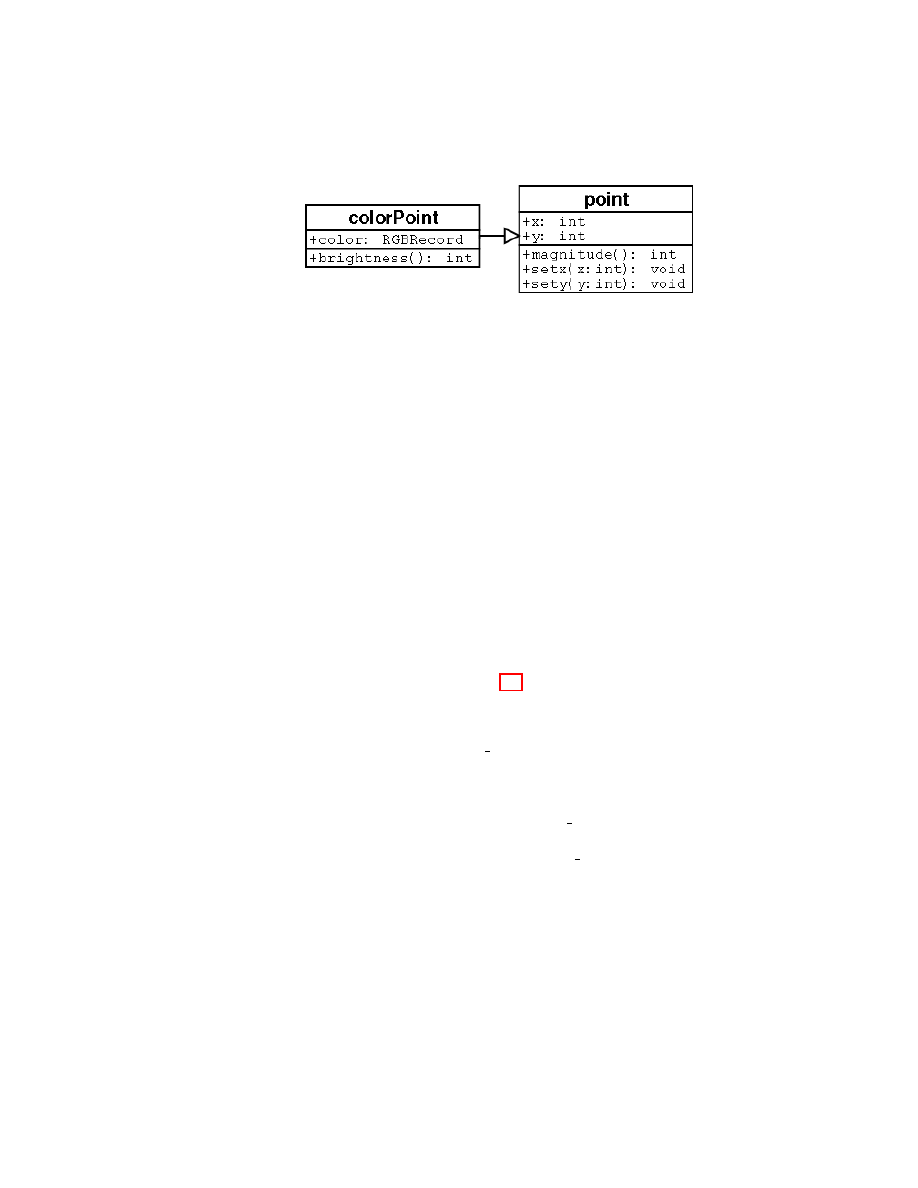
78
CHAPTER 5. OBJECT-ORIENTED LANGUAGE FEATURES
Figure 5.3: The point, colorPoint inheritance hierarchy.
• Objects that encapsulate data and code under a single name to achieve
certain functionality.
• Polymorphic objects.
• Templates for generating objects (the main function of classes)
The other 20 percent of the utility comes from from inheritance. Inheri-
tance allows related objects to be defined that share some common code. Inher-
itance can be encoded in F[SR by using the following scheme. In the subclass,
we create an instance of the superclass object, and keep the instance around
as a “slave.” We use the slave to access methods and fields of the superclass
object. Thus, the subclass object only contains new and overridden methods.
Real object oriented languages tend not to implement inheritance this way for
reasons of efficiency (imagine a long inheritance chain in which a method call
has to be delegated all the way back to the top of the hierarchy before it can
be invoked). Still, the encoding is good enough to illustrate the main points
of inheritance. For example, consider the following encoding of ColorPoint, a
subclass of Point, illustrated in Figure 5.3.
Let pointClass = . . . In
Let colorPointClass = Function
->
Let super = pointClass {} In {
x = super.x; y = super.y;
color = Ref {red = 45; green = 20; blue = 20};
magnitude = Function this -> Function
->
mult(super.magnitude this {})(this.brightness this {});
brightness = Function this -> Function
->
(* compute brightness. . . *)
setx = super.setx; sety = super.sety
} In . . .
There are several points of interest in this encoding. First of all, notice
that to inherit methods and fields from the superclass, we explicitly link them
together (i.e. x, y, setx, and sety). To override a method in the superclass, we
simply redefine it in the subclass instead of linking to the superclass; magnitude

5.1. ENCODING OBJECTS IN F[SR
79
is an example of this. Also notice that we can still invoke superclass methods
from the subclass. For instance, magnitude invokes super.magnitude in its
body. Notice how super.magnitude is passed this instead of super as its
argument. This has to do with dynamic dispatch, which we will address now.
5.1.6
Dynamic Dispatch
We say that a method is dynamically dispatched if, looking at a message send
v<-m, we are not sure precisely what method m will be executed at runtime.
Dynamic dispatch is related to object polymorphism: a variable v could contain
many different kinds of objects, so v<-m could be sending m to any one of those
different kinds of objects. Unless we know what kind of objects v is at runtime,
we cannot know which method m will be invoked.
The term dynamic dispatch refers to how the method invoked by a message
send is not fixed at compile-time.
If we had a method isNull declared in
pointClass and inherited by colorPointClass with code
Function this -> Function
-> (this.magnitude this {}) = 0,
the magnitude method here is not fixed at compile-time. If this is a point, it
will use point’s magnitude method. If it’s a colorPoint, that colorPoint’s
overridden magnitude method will be used.
To illustrate the difference between static and dynamic dispatch, let us con-
sider a new example. Consider the following classes, rectClass and its subclass
squareClass.
Let rectClass = Function
-> {
getWidth = Function this -> Function
-> 10;
getLength = Function this -> Function
-> 1;
area = Function this -> Function
->
mult ((this.getLength) this {}) ((this.getWidth) this {})
} In
Let squareClass = Function
->
Let super = rectClass {} In {
getLength = (super.getLength);
(* We override width to be the same as length *)
getWidth = (super.getLength);
areaStatic = Function this -> Function
->
(super.area) super {};
areaDynamic = Function this -> Function
->
(super.area) this {}

80
CHAPTER 5. OBJECT-ORIENTED LANGUAGE FEATURES
} In \ldots
Notice that in the squareClass, getLength has been overridden to be-
have the same as getWidth.
There are two ways to calculate the area in
squareClass.
areaStatic calls (super.area) super {}.
This means that
when rectClass’s area method is invoked, it is invoked with rectClass’s
getLength and getWidth as well. The result is 1 × 10, which is 10.
On the contrary, the dynamically dispatched area method, areaDynamic
is written (super.area) this {}. This time, rectClass’s area method is
invoked, but this is an instance of squareClass, rather than rectClass, and
squareClass’s overridden getLength and getWidth are used. The result is 1,
the correct area for a square. The behavior of dynamic dispatch is almost always
the behavior we want. The key to dynamic dispatch is that inherited methods
get a revised notion of this when they are inherited. Our encoding promotes
dynamic dispatch, because we explicitly pass this into our methods.
Java (and almost every other object-oriented language) uses dynamic dis-
patch to invoke methods by default. In C
++
, however, unless a method is de-
clared as virtual, it will not be dynamically dispatched.
5.1.7
Static Fields and Methods
Static fields and methods are found in almost all object-oriented languages, and
are simply fields and methods that are not tied to a particular instance of an
object, but rather to the class itself.
We can trivially encode static fields and methods by simply making our
class definitions records instead of functions. The creation of the object can
itself be a static method of the class. This is, in fact, how Smalltalk implements
constructors. Consider the following reimplementation of pointClass in which
we make use of static fields.
Let pointClass = {
newWithXY = Function class ->
Function newx ->
Function newy -> {
x = Ref newx;
y = Ref newy;
magnitude = Function this -> Function
->
sqrt ((!(this.x)) + (!(this.y)))
};
new = Function class -> Function
->
(class.newWithXY) class (class.xdefault)
(class.ydefault);

5.2. THE F[OB LANGUAGE
81
xdefault = 4;
ydefault = 3
} In
Let point = (pointClass.new) pointClass {} In
(point.magnitude) point {}
Notice how the class method newWithXY is actually responsible for building
the point object.
new simply invokes newWithXY with some default values
that are stored as class fields. This is a very clean way to encode multiple
constructors.
Perhaps the most interesting thing the encoding is how classes with static
fields start to look like our original encoding of simple objects. Look closely—
notice that class methods take an argument class as their first parameter, for
the exact same reason that regular methods take this as a parameter. So in
fact, pointClass is really just another primitive object that happens to be able
to create objects.
Viewing classes as objects is the dominant paradigm in Smalltalk. Java has
some support for looking at classes as objects through the reflection API as well.
Even in languages like C
++
that don’t view classes as objects, design patterns
such as the Factory patterns[11] capture this notion of objects creating objects.
This encoding is truly in the spirit of object-oriented programming, and
it is a clean, and particularly satisfying way to think about classes and static
members.
5.2
The F[OB Language
Now that we have looked at encodings of objects in terms of the known syntax of
F[SR, we may now study how to add these features directly to a language. We
will call this language F[OB, F[ with objects. Our encodings of objects were
operationally correct, but not adding syntactic support for objects makes them
too difficult to work with in practice. The colorPoint encoding, for example,
is quite difficult to read. This readability problem only gets worse when types
are introduced into the language.
F[OB includes the most of the features we discussed above: classes, message
send, methods, fields, super, and this.
We support information hiding in
the same manner in which Smalltalk does: all instance variables are hidden
(protected) and all methods are exposed (public).
F[OB also supports primitive objects. Primitive objects are objects that
are defined “inline,” that is, objects that are not created from a class. They
are a more lightweight from of object, and are similar to Smalltalk’s blocks and
Java’s anonymous classes. Primitive objects aren’t very common in practice,

82
CHAPTER 5. OBJECT-ORIENTED LANGUAGE FEATURES
but we include them in F[OB because it requires very little work. The value
returned by the expression new aClass is an object, which means that an object
is a first class expression. As long as our concrete syntax allows us to directly
define primitive objects, no additional work is needed in the interpreter.
An interesting consequence of having primitive objects is that is that we
could get rid of functions entirely (not methods). Functions could simply be
encoded as methods of primitive objects. For this reason, object-oriented lan-
guages that support primitive objects have many of the advantages of higher-
order functions.
5.2.1
Concrete Syntax
Let’s introduce the F[OB concrete syntax with an example. The following
code is an implementation of the pointClass / colorPointClass hierarchy
from before (Figure 5.3).
Let pointClass =
Class Extends EmptyClass
Inst
x = 3;
y = 4
Meth
magnitude = Function
-> sqrt(x + y);
setx = Function newx -> x := newx;
sety = Function newy -> y := newy
In Let colorPointClass =
Class Extends pointClass
Inst
x = 3;
y = 4;
(* A use of a primitive object: *)
color = Object
Inst
Meth red = 45; green = 20; blue = 20
Meth
magnitude =
Function
->
mult(Super <- magnitude {})(This <- brightness)
(* An unnormalized brightness metric *)
brightness = Function
->
color <- red + color <- green + color <- blue;
setx = Super <- setx (* explicitly inherit *)
sety = ...; setcolor = ...
In Let point = New pointClass

5.2. THE F[OB LANGUAGE
83
In Let colorPoint = New colorPointClass In
(* Some sample expressions *)
point <- setx 4;
point <- magnitude{};
colorpoint <- magnitude {}
There is a lot going on with this syntax, so let’s take some time to point out
some of the major elements. First of all, notice that This and Super are special
“reserved variables.” In our F[ encodings, we had to write “Function this
-> ” and pass this as an explicit parameter.
Now, self-awareness happens
implicitly, and is This is a reference to self.
Note the use of a primitive object to define the color field of the color-
PointClass. The red, green, and blue values are implemented as methods,
since fields are always “private.”
In our previous encodings we used one style when defining the base class, and
another different style when defining the subclass. In F[OB we use the same
syntax for both by always specifying the superclass. To allow for base classes
that do not inherit from any other class, we allow a class to extend EmptyClass,
which is simply an special class that does not define anything.
F[OB instance variables use the l/r-value form of state that was discussed
in Section 4.1.3. There is no need to explicitly use the ! operator to get the
value of an instance variable. F[OB instance variables are therefore mutable,
not following the Caml convention that all variables are immutable. Note that
method arguments are still immutable. There are thus two varieties of vari-
able: immutable method parameters, and mutable instances. Since it is clear
which variables are instances and which are not, there is no great potential for
confusion. It is the job of the parser to distinguish between instance variables
and regular variables. An advantage of this approach is that it keeps instance
variables from being directly manipulated by outsiders.
Method bodies are generally functions, but need not be; they can be any
immutable, publicly available value. For example, immutable instances can be
considered methods (see the color primitive object in the example above).
Note that we still have to explicitly inherit methods. This is not the cleanest
syntax, but it simplifies the interpreter, and makes facilitates translation to
F[SR discussed in Section 5.2.3.
Also, there is no constructor function. new is used to create new instances,
and, following Smalltalk, initialization is done explicitly by writing an initialize
method.
For simplicity, F[OB does not support static fields and methods, nor does
it take the “classes as objects” view discussed in the previous section.
5.2.2
A Direct Interpreter
We first consider a direct interpreter for F[OB. The abstract syntax can be
expressed by the following Caml type.

84
CHAPTER 5. OBJECT-ORIENTED LANGUAGE FEATURES
type ide = Ide of string | This | Super
type label = Lab of string
type expr = (* the F[ expressions, including Let *)
(* Object holds the instance list and the method list *)
| Object of ((label * expr) list) * ((label * expr) list)
| Class of expr * ((label * expr) list) * ((label * expr) list)
| EmptyClass
| New of expr
| Send of
expr * label
(* parser has to decide if a var. is InstVar or just a Var *)
| InstVar of label
| InstSet of label * expr
Here is a rough sketch of the interpreter. This interpreter is not complete, but
it gives a general idea of what one should look like.
(* Substitute "sinst" for Super in all method bodies *)
let rec subst_super sinst meth =
match meth with
[] -> []
| (l, body)::rest ->
(l, subst(body, InstVar(sinst), Super))::
(subst_super sinst rest)
let rec eval e =
match e with
...
| Object(inst, meth) -> Object(eval_insts inst, meth)
| Send(term1, label) ->
(match (eval term1) with
Object(inst, meth) ->
subst(selectMeth(meth, label),
Object(inst, meth), This)
_ -> raise TypeMismatch)
| Class(super, inst, meth) -> Class(super, inst, meth)
| New(Class(super, inst, meth) ->
(match super with
EmptyClass -> eval (Object(inst, meth))
| s -> let sobj = eval(New super) in
let sinst = (* A fresh instance variable label *) in
let newinst = (sinst, sobj)::inst in
let newmeth = subst_super sinst meth in
eval (Object(newinst, newmeth))
...

5.2. THE F[OB LANGUAGE
85
and eval_insts inst =
match inst with
[] -> []
| (l, body)::rest -> (l, eval(body))::(eval_insts rest)
This code sketch for the interpreter does a nice job of illustrating the roles of
This and Super. We only substitute for this when we send a message. That’s
because This is a dynamic construct, and we don’t know what it will be until
runtime (see the discussion of dynamic dispatching in Section 5.1.6). On the
other hand, Super is a static construct, and is known at the time we write the
code, which allows us to substitute for Super as soon as the Class expression
is evaluated.
5.2.3
Translating F[OB to F[SR
Another way to give meaning to F[OB programs is by defining a translation
mapping F[OB programs into F[SR programs. This is a complete characteri-
zation of how objects can be encoded in F[SR, the topic of Section 5.1.
In Chapter 7 below, we devleop a compiler for F[SR. To obtain a compiler
for F[OB, we can simply add a translation step that translates F[OB to F[SR,
and then simply compile the F[SR using this compiler. Thus, we will have a
F[OB compiler “for free” when we are all done. This section only discusses the
F[OB to F[SR translation.
The translation is simply a formalization of the encodings given in Sec-
tion 5.1. Although real object-oriented compilers are much more sophisticated,
this section should at least provide an understandable view of what an object-
oriented compiler does. The concrete syntax translation is inductively defined
below in a piecewise manner.

86
CHAPTER 5. OBJECT-ORIENTED LANGUAGE FEATURES
toDSR(Object Inst x
1
=e
1
; . . . ; x
n
=e
n
Meth m
1
=e
0
1
; . . . ; m
k
=e
0
k
) =
{inst = {x
1
=Ref(toDSR(e
1
)); . . . ; x
n
=Ref(toDSR(e
n
))};
meth = {m
1
= Function this -> toDSR(e
0
1
); . . . ;
m
k
= Function this -> toDSR(e
0
k
)} }
toDSR(Class Extends e Inst x
1
=e
1
; . . . ; x
n
=e
n
Meth m
1
=e
0
1
; . . . ; m
k
=e
0
k
) =
Function
-> Let super = (toDSR(e)) {} In
{inst = {x
1
=Ref(toDSR(e
1
)); . . . ; x
n
=Ref(toDSR(e
n
))};
meth = {m
1
= Function this -> toDSR(e
0
1
); . . . ;
m
k
= Function this -> toDSR(e
0
k
)} }
toDSR(New e) = (toDSR(e)) {}
toDSR(EmptyClass) = Function
-> {}
toDSR(Super <- m args) = super.meth.m this args
toDSR(e <- m args) =
Let ob = toDSR(e) In ob.meth.m ob args, for e not Super
toDSR(x := e) = this.inst.x := toDSR(e)
toDSR(x) = !(this.inst.x), for x an instance variable
toDSR(y) = y, for y a function variable
toDSR(anything else) = homomorphic
The translation is fairly clean, except that messages to Super have to be
handled a bit differently that other messages in order to properly implement
dynamic dispatch. Notice again that instance variables are handled differently
than function variables, because they are mutable. Empty function application,
i.e. f (), may be written as empty record application: f {}. The “ ” variable
in Function
-> e is any variable not occurring in e. The character “ ” itself
is a valid variable identifier in the DDK implementation of F[SR, however (see
Chapter A).
As an example of how this translation works, let us perform it on the F[OB
version of the point / colorPoint classes from Section 5.2.1. The result is the
following:
Let pointClass =
Function
-> Let super = (Function
-> {}) {} In {
inst = {
x = Ref 3;
y = Ref 4
};
meth = {
magnitude = Function this -> Function
->
sqrt ((!(this.inst.x)) + (!(this.inst.y)));
setx = Function this -> Function newx ->
(this.inst.x) := newx;
sety = Function this -> Function newy ->

5.2. THE F[OB LANGUAGE
87
(this.inst.y) := newy
}
}
In Let colorPointClass =
Function
-> Let super = pointClass {} In {
inst = {
x = Ref 3;
y = Ref 4;
color = Ref ({inst = {}; meth = {
red = Function this -> 45;
green = Function this -> 20;
blue = Function this -> 20
}})
};
meth = {
magnitude = Function this -> Function
->
mult ((super.meth.magnitude) this {})
((this.meth.brightness) this {});
brightness = Function this -> Function
->
(((!(this.inst.color)).meth.red) this) +
(((!(this.inst.color)).meth.green) this) +
(((!(this.inst.color)).meth.blue) this);
setx = Function this -> Function newy ->
(super.meth.setx) this newy;
sety = Function this -> Function newy ->
(super.meth.setx) this newy;
setcolor = Function this -> Function c ->
(this.inst.color) := c
}
} In
(* Let colorPoint = New colorPointClass In
*
colorPoint <- magnitude {}
*)
Let colorPoint = colorPointClass {} In
(colorPoint.meth.magnitude) colorPoint {};;
Interact with F[SR. The translated code above should run fine in
F[SR, provided you define the mult and sqrt functions first. mult is
easily defined as
Let Rec mult x = Function y ->
If y = 0 Then
0
Else
88
CHAPTER 5. OBJECT-ORIENTED LANGUAGE FEATURES
x + (mult x (y - 1)) In ...
sqrt is not so easily defined. Since we’re more concerned with the behavior of
the objects, rather than numerical accuracy, just write a dummy sqrt function
that returns its argument:
Let sqrt = Function x -> x In ...
Now, try running it with the F[SR file-based interpreter. Our dummy sqrt
function returns 7 for the point version of magnitude, and the colorPoint
magnitude multiplies that result by the sum of the brightness (85 in this case).
The result is
$ DSR dobDsr.dsr
==> 595
After writing a Caml version of toDSR for the abstract syntax, a F[OB
compiler is trivially obtained by combining toDSR with the functions defined
in Chapter 7:
let DOBcompile e = toC(hoist(atrans(clconv(toDSR e))))
Finally, there are several other ways to handle these kinds of encodings.
More information about encoding objects can be found in [9].

Chapter 6
Type Systems
In F[, if we evaluate the expression
3 + (If False Then 3 Else False),
we will get some kind of interpreter-specific error at runtime. If F[ had a type
system, such an expression would not have been allowed to evaluate.
In Lisp, if we define a function
(defun f (x) (+ x 1)),
and then call (f "abc"), the result is a runtime type error. Similarly, the
Smalltalk expression
String new myMessage
results in a “message not supported” exception when run. Both of these runtime
errors could have been detected before runtime if the languages supported static
type systems.
The C
++
code
int a[10]; a[123] = 5;
executes unknown and potentially harmful effects, but the equivalent Java code
will throw an ArrayIndexOutOfBoundsException at runtime, because array
access is checked by a dynamic type system.
89
90
CHAPTER 6. TYPE SYSTEMS
These are just a few examples of the kinds of problems that type systems
are designed to address. In this chapter we discuss such type systems, as well
as algorithms to infer and to check types.
6.1
An Overview of Types
A type is simply a property with which a program is implicitly or explicitly
annotated before runtime. Type declarations are invariants that hold for all
executions of a program, and can be expressed as statements such as “this
variable always holds a String object,” or “this function always returns a tree
expression.”
Types have many other advantages besides simply cutting down on runtime
errors. Since types (and module signatures) specify invariant properties of the
program, they serve as precise and descriptive comments on the functionality
of the code. In this manner, types aid in large software development.
With a typed language, more information is known at compile-time, and
this helps the compiler produce much faster code. For example, the record
implementation we will use in our F[SR compiler (via hashing, see Chapter 7)
is not needed in C
++
due to its static type system. We know the size of all
records at compile-time, and therefore know where they should be laid out in
memory. In contrast, Smalltalk is very slow, and the lack of a static type system
counts for much of the slowness. The Strongtalk system [7] attempts to bring a
static type system into Smalltalk.
Finally, in an untyped language its easier to do very ugly “hacking”. For
instance, a list [1;true;2;false;3;true] can be written in an untyped lan-
guage, but this is dangerous and it would be much preferred to represent this
as [(1,true);(2,false);(3,true)], which, in Caml, has the type (int *
bool) list.
However, untyped languages have one distinct advantage over typed ones:
they are more expressive. For example, consider the F[SR encoding of F[OB
from Chapter 5. This encoding would not work with Caml as the target lan-
guage, because the Caml type system disallows record polymorphism.
The
Y -combinator is another example of where an untyped language really shines.
F[ could support recursion via the Y -combinator, but a simple typed version of
F[ can’t since it cannot be typed. Recall from Section 2.3.5 that Caml can not
type the Y -combinator, either.
All of us have seen types used in many ways. The following is a list of some
of the more common dimensions of types.
• Atomic types: int, float, . . .
• Type constructors, which produce types from types: ’a -> ’b, ’a * ’b
• Caml-style type constructor definitions via type
• C-style type definitions via struct and typedef

6.1. AN OVERVIEW OF TYPES
91
• Object-oriented types: class types, object types
• Module types, or signatures
• Java-style interfaces
• Exception types: hmethodi throws hexceptioni
• Parametric polymorphism: ’a -> ’a
• Record/Object polymorphism: pass a ColorPoint to a function which
expects a Point.
There are also several newer dimensions of types that are currently active re-
search areas.
• Effect types: the type “int -x,y-> int” indicates that variables x and
y will assigned to in this function. Java’s throws clauses for methods are
a form of effect types.
• Concrete class analysis: for variable x:Point, a concrete class analysis
produces a set such as {Point, ColorPoint, DataPoint}. This means at
runtime x could either be a Point, a ColorPoint, or a DataPoint (and,
nothing else). This is useful in optimization.
• Typed Assembly Language [2, 17]: put types on assembly-level code and
have a type system that guarantees no unsafe pointer operations.
• Logical assertions in types: int -> { x:int | odd(x) } for a function
returning odd numbers.
There is an important distinction that needs to be made between static and
dynamic type systems. Static type systems are what we usually mean when
we talk about type systems. A static type system is the standard notion of
type found in C, C
++
, Java and Caml. Types are checked by the compiler, and
type-unsafe programs fail to compile.
Dynamic type systems, on the other hand, check type information at
runtime. Lisp, Scheme, and Smalltalk are, in fact, dynamically typed. In fact,
F[ and F[SR are technically dynamically typed as well, since they will raise a
typeMismatch when the type of an expression is not what it expects. Any time
you use a function, the runtime environment makes sure that its a function. If
you use an integer, it makes sure it’s an integer, etc. These runtime type checks
add a lot of overhead to the runtime environment, and thus cause programs to
run slowly.
There is some dynamic typechecking that occurs in statically typed lan-
guages too. For instance, in Java, downcasts are verified at run-time and can
raise exceptions. Out-of-bounds array accesses are also checked at run-time in
Java and Caml, and are thus dynamically typed. Array accesses are not typed
in C or C
++
, since no check is performed at all. Note that the type of an array
(i.e. int, float) is statically checked, but the size is dynamically checked.

92
CHAPTER 6. TYPE SYSTEMS
Finally, languages can be untyped. The DSR compiler produces untyped
code, since runtime errors cause core dumps. It is important to understand the
distinction between an untyped language and a dynamically typed one. In an
untyped language there is no check at all and anomalous behavior can result
at runtime. In Chapter 7, we compile F[SR to untyped C code, using casts
to “disable” type system. Machine language is another example of an untyped
language.
To really see the difference between untyped and dynamically typed lan-
guages, consider the following two program fragments. The first is C
++
code
with the type system “disabled” via casts.
#include <iostream>
class Calculation {
public: virtual int f(int x) { return x; }
};
class Person {
public: virtual char *getName() { return "Mike"; }
};
int main(int argc, char **argv) {
void *o = new Calculation();
cout << ((Person *)o)->getName() << endl;
return 0;
}
The code compiles with no errors, but when we run it the output is “˜
a¿.”
But if we compile it with optimization, the result is “ ˜
A`
a.” Run it on a different
computer and it may result in a segmentation fault. Use a different compiler,
and the results may be completely exotic and unpredictable. The point is that
because we’re working with an untyped language, there are no dynamic checks
in place, and meaningless code like this results in undefined behavior.
Contrast this behavior with that of the equivalent piece of Java code. Recall
that Java’s dynamic type system checks the type of the object when a cast is
made. We will use approximately the same code:
class Calculation {
public int f(int x) { return x; }
}
class Person {
public String getName() { return "Mike"; }
}

6.2. TF[: A TYPED F[ VARIATION
93
class Main {
public static void main(String[] args) {
Object o = new Calculation();
System.out.println(((Person) o).getName());
}
}
When we run this Java code, the behavior is quite predictable.
Exception in thread "main" java.lang.ClassCastException: Calculation
at Main.main(example.java:12)
The ClassCastException is an exception raised by Java’s dynamic type
system. The unsafe code is never executed in Java, and so the behavior of the
program is consistent and well-defined. With the C
++
version, there is no dy-
namic check, and the unsafe code is executed, resulting in wild and unexpected
behavior.
6.2
TF[: A Typed F[ Variation
We will use the prefix “T” to represent a typed version of a language which we
have previously studied. Thus we have several possible languages: TF[, TDS,
TDS, TDSR, TDOB, TDX, TF[SRX, etc. There are too many languages
to consider individually, so we will first look at TF[ as a warm-up, and then
consider full-blown TF[SRX.
6.2.1
Design Issues
Before we begin to investigate TF[ or any typed language, there are a few
general design issues to address. We will take a moment to discuss these issues
before giving the specification for TF[.
The first question to ask is how much explicit type information must our
language contain? How much type information must the program be decorated
with, and how much can be inferred by the compiler? A spectrum of possibilities
exists.
On one end of the spectrum, we can use no decoration at all. We simply
stick to our untyped language syntax, and let the compiler infer all the type
information.
Alternatively, we can use limited decoration, and have the compiler do partial
inference. There is a wide range of possibilities. C for instance requires function
argument and return types to be specified, and declared variables to be given
types. However, within the body of a function, individual expressions do not
need to be typed as those types may be inferred. Some languages only require
function argument types be declared, and the return values of functions is then
inferred.

94
CHAPTER 6. TYPE SYSTEMS
At the other end of the spectrum, every subexpression and its identifier
must be decorated with its type. This is too extreme, however, and makes the
language unusable. Instead of writing
Function x -> x + 1,
we would need some gross syntax like
(Function x -> (x:int + 1:int):int):(int -> int).
For TF[ and TF[SRX, we will concentrate on the C and Pascal view of
explicit type information. We specify function argument and return types, and
declared variable types, and allow the rest to be inferred.
We should also illustrate the difference between type checking and type
inference. In any typed language, the compiler should typecheck the program
before generating code. Type inference algorithms infer types and check
that the program body has no type errors. Caml is an example of this.
A type checker generally just checks the body is well-typed given the types
listed on declarations. This is how C, C
++
, and Java work, although technically
they are also inferring some types, such as the type of 3+4.
In any case it must be possible to run the type inference or type checking
algorithm quickly. Caml in theory can take exponential time to infer types, but
in practice it is linear.
6.2.2
The TF[ Language
Finally, we are ready to look at TF[, a typed F[ language. To simplify things, we
will not include the Let Rec syntax of F[, but only non-recursive, anonymous
functions. We will discuss typing recursion in Section 6.4.
In analogue with our development of operational semantics and interpreters,
we will define two things when discussing types. First we define type sys-
tems, which are language-independent notations for assigning types to pro-
grams. Type systems are analogous to operational semantics. Secondly, we
define type checkers, which are Caml implementations of type systems anal-
ogous to interpreters. We begin with type systems.
Type Systems
Type systems are rule-based formal systems that are similar to operational
semantics. Type systems rigorously and formally specify what program have
what types, and have a strong and deep parallel with formal logic (recall our
discussion of Russell’s Paradox in Section 2.3.5). Type systems are generally a
set of rules about type assertions.

6.2. TF[: A TYPED F[ VARIATION
95
Definition 6.1. (Type Environment) A type environment, Γ, is a set {x
1
:
τ
1
, . . . , x
n
: τ
n
} of bindings of free variables types. If a variable x is listed twice
in Γ, the rightmost (innermost) binding is the proper type. We write Γ(x) = τ
to indicate that τ is the innermost type for x in Γ.
Definition 6.2. (Type Assertion) A type assertion, Γ ` e : τ , indicates that
in type environment Γ, e is of type τ .
The TF[ types in the concrete syntax are
τ ::= Int | Bool | τ -> τ.
We can represent this in a Caml abstract syntax as
type dtype = Int | Bool | Arrow of dtype * dtype
The expressions of TF[ are almost identical to those of F[, except that we
must explicitly decorate functions with type information about the argument.
For example, in the concrete syntax we write
Function x:τ -> e
where the abstract syntax representation is
Function of ide * dtype * expr
The TF[ Type Rules
We are now ready to define the TF[ types rules. These rules have the same
structure as the operational semantics rules we have looked at before; the hor-
izontal line reads “implies.” The following three rules are the axioms for out
type system (recall that an axiom is a rule that is always true, that is, a rule
with nothing above the line).
(Hypothesis)
Γ ` x : τ for Γ(x) = τ
(Int)
Γ ` n : Int for n an integer
(Bool)
Γ ` b : Bool for b True or False

96
CHAPTER 6. TYPE SYSTEMS
The Hypothesis rule simply says that if a variable x contained in a type
environment Γ has type τ then the assertion Γ ` x : τ is true. The Int and
Bool rules simply give types to literal expressions such as 7 and False. These
rules make up the base cases of our type system.
Next, we have rules for simple expressions.
(+)
Γ ` e : Int, Γ ` e
0
: Int
Γ ` e + e
0
: Int
(-)
Γ ` e : Int, Γ ` e
0
: Int
Γ ` e - e
0
: Int
(=)
Γ ` e : Int, Γ ` e
0
: Int
Γ ` e = e
0
: Bool
These rules are fairly straightforward. For addition and subtraction, the
operands must typecheck to Ints, and the result of the expression is an Int.
Equality is similar, but typechecks to a Bool. Note that equality will only
typecheck with integer operands, not boolean ones. The And, Or, and Not rules
are similar, and their definition should be obvious.
The If rule is a bit more complicated. Clearly, the conditional part of
the expression must typecheck to a Bool. But what about the Then and Else
clauses. Consider the following expression.
If e Then 3 Else False
Should this expression typecheck? If e evaluates to True, then the result is 3,
an Int. If e is False, the result is False, a Bool. Clearly, then this expression
should not typecheck, because it does not always evaluate to the same type. This
tells us that for an If statement to typecheck, both clauses must typecheck to
the same type, and the type of the entire expression is then the same as the two
clauses. The rule is as follows.
(If)
Γ ` e : Bool, Γ ` e
0
: τ, Γ ` e
00
: τ,
Γ ` If e Then e
0
Else e
00
: τ
We have now covered all the important rules except for functions and appli-
cation. The Function rule is a bit different from other rules, because functions
introduce new variables. The type of the function body depends on the type
of the variable itself, and will not typecheck unless that variable is in Γ, the
type environment. To represent this in our rule, we need to perform the type
assertion with the function’s variable appended to the type environment. We
do this in the following way.

6.2. TF[: A TYPED F[ VARIATION
97
(Function)
Γ, x : τ ` e : τ
0
Γ ` (Function x:τ -> e) : τ -> τ
0
Notice the use of the type constructor -> to represent the type of the entire
function expression. This type constructor should be familiar, as the Caml type
system uses the same notation. In addition, the Function rule includes the
addition of an assumption to Γ. We assume the function argument, x, is of type
τ , and add this assumption to the environment Γ to derive the type of e. The
Application rule follows from the Function rule:
(Application)
Γ ` e : τ -> τ
0
, Γ ` e
0
: τ
Γ ` e e
0
: τ
0
Just as in operational semantics, a derivation of Γ ` e : τ is a tree of rule
applications where the leaves are axioms (Hypothesis, Int or Bool rules) and
the root is Γ ` e : τ .
Let’s try an example derivation.
` (Function x:Int -> (Function y:Bool ->
If y Then x Else x+1)) :
Int -> Bool -> Int
Because by the function rule, it suffices to prove
x : Int ` (Function y:
Bool -> (If y Then x Else x+1)) :
Bool->Int
Because by the function rule again, it suffices to prove
x : Int, y : Bool ` If y Then x Else x+1 : Int
Because by the If rule, it suffices to prove
x : Int, y : Bool ` y : Bool
x : Int, y : Bool ` x : Int
x : Int, y : Bool ` x+1 : Int
all of which either follow by the Hypothesis rule or + and
Hypothesis.
Given the above and letting
f = (Function x:Int -> (Function y:Bool ->
If y Then x Else x+1
we then have

98
CHAPTER 6. TYPE SYSTEMS
` f 5 True : Int
Because by the application rule,
` f : Int -> Bool -> Int
(which we derived above)
` 5 : Int by the Int rule
And thus
` f 5 : Bool -> Int by the Application rule.
Given this and
` True : BoolbytheBoolrule
we can get
` f 5 True : Int by the Application rule.
As we mentioned before, TF[ is a very weak language. No recursive functions
can be defined.
In fact, all programs are guaranteed to halt.
TF[ is thus
normalizing. Without recursion, TF[ is not very useful. Later we will add
recursion to TF[SRX and show how to type it.
Exercise 6.1. Try to type the Y -combinator in TF[.
Now that we have a type system for the TF[ language, what can we do
with it. We can detect whether or not our programs are well-typed, but what
does it mean if they are. The answer comes in the form of the following type
soundness theorem.
Theorem 6.1. If ` e : τ , then in the process of evaluating e, a “stuck state” is
never reached.
We will not precisely define the concept of a stuck state. It is basically a
point at which evaluation can not continue, such as 0 (Function x -> x) or
(Function x -> x) + 4. In terms of a F[ interpreter, stuck stated are the
cases that raise exceptions. This theorem asserts that a type system prevents
runtime errors from occurring.
Similar theorems are the goal of most type
systems.
6.3
Type Checking
To write an interpreter for TF[, we simply modify the F[ interpreter to ig-
nore type information at runtime. What we are really interested in is writing a
type checker. This is the type system equivalent of an interpreter; given the
language-independent type rules, define a type checking algorithm in a partic-
ular language, namely Caml.
A type-checking algorithm typeCheck, takes as input a type environment Γ
and expression e as and either return its type, τ , or raises an exception indicating
e is not well-typed in the environment Γ.

6.4. TYPES FOR AN ADVANCED LANGUAGE: TF[SRX
99
Some type systems do not have an easy corresponding type-checking algo-
rithm. In TF[ we are fortunate in that the type checker mirrors the type rules
in a nearly direct fashion. As was the case with the interpreters, the outermost
structure of the expression dictates the rule that applies. The flow of the recur-
sion is that we pass the environment Γ and expression e down, and return the
result type τ back up.
Here is a first pass at the TF[ typechecker, typecheck :
envt * expr ->
dtype. Γ can be implemented as a (ide * dtype) list, with the most recent
item at the front of the list.
let rec typecheck gamma e =
match e with
(* look up first mapping of x in list gamma *)
Var x -> lookup gamma x
| Function(Ide x,t,e) ->
let t’ = typecheck (((Ide x),t)::gamma) e in
Arrow(t,t’)
| Appl(e1,e2) ->
let Arrow(t1,t2) = typecheck gamma e1 in
if typecheck gamma e2 = t1 then
t2
else
raise TypeError
| Plus(e1,e2) ->
if typecheck gamma e1 = Int and
typecheck gamma e2 = Int then
Int
else
raise TypeError
| (* \ldots *)
Lemma 6.1. typecheck faithfully implements the TF[ type system. That is,
• ` e : τ if and only if typecheck [] e returns τ , and
• if typecheck [] e raises a typeError exception, ` e : τ is not provable
for any τ .
Proof. Omitted (by case analysis).
This Lemma implies the typecheck function is a sound implementation of the
type system for TF[.
6.4
Types for an Advanced Language: TF[SRX
Now that we’ve looked at a simple type system and type checker, let us move
on to a type system for a more complicated language: TF[SRX. We include

100
CHAPTER 6. TYPE SYSTEMS
just about every piece of syntax we have used up to now, except for F[OB’s
classes and objects and F[V’s variants. Here is the abstract syntax defined in
terms of a Caml type.
type expr =
Var of ident
| Function of ident * dtype * expr
| Letrec of ident * ident * dtype * expr * dtype * expr
| Appl of expr * expr
| Plus of expr * expr | Minus of expr * expr
| Equal of expr * expr | And of expr * expr
| Or of expr * expr | Not of expr
| If of expr * expr * expr | Int of int | Bool of bool
| Ref of expr | Set of expr * expr | Get of expr
| Cell of int | Record of (label * expr) list
| Select of
label * expr | Raise of expr * dtype |
| Try of expr * string * ident * expr
| Exn of string * expr
and dtype =
Int | Bool | Arrow of dtype * dtype
| Rec of label * dtype list | Rf of dtype | Ex of dtype
Next, we will define the type rules for TF[SRX. All of the TF[ type rules
apply, and so we can move directly to the more interesting rules. Let’s begin
by tackling recursion. What we’re really typing is the In clause, but we need to
ensure that the rest of the expression is also well-typed.
(Let Rec)
Γ, f : τ -> τ
0
, x : τ ` e : τ
0
,
Γ, f : τ -> τ
0
` e
0
: τ
00
Γ ` (Let Rec f x:τ = e:τ
0
In e
0
) : τ
00
Next, we move on to records and projection. The type of a record is simply
a map of the field names to the types of the values associated with each field.
Projection is typed as the type of the value of the field projected. The rules are
(Record)
Γ ` e
1
: τ
1
, . . . , Γ ` e
n
: τ
n
Γ ` {l
1
= e
1
; . . . ; l
n
= e
n
} : {l
1
: τ
1
; . . . ; l
n
: τ
n
}
(Projection)
Γ ` e : {l
1
: τ
1
; . . . ; l
n
: τ
n
}
Γ ` e.l
i
: τ
i
for 1 ≤ i ≤ n
We’ll also need to be able to type side effects. We can type Ref expressions
with the special type τ Ref. Set and Get expressions easily follow.

6.4. TYPES FOR AN ADVANCED LANGUAGE: TF[SRX
101
(Ref)
Γ ` e : τ
Γ ` Ref e : τ Ref
(Set)
Γ ` e : τ Ref, Γ ` e
0
: τ
Γ ` e := e
0
: τ
(Get)
Γ ` e : τ Ref
Γ ` !e : τ
Finally, the other kind of side effects we need to type are exceptions. To type
an exception itself, we will simply use the type Exn. This allows all exceptions
to be typed in the same way. For example, the code
If b Then (#IntExn 1) Else (#BoolExn False)
will typecheck, and has type Exn. We do this to allow maximum flexibility.
Because they alter the flow of evaluation, Raise expressions should always
typecheck, provided the argument typechecks to an Exn type. It is difficult
to know what type to give a raise expression, though. Consider the following
example.
If b Then Raise (#Exn True) Else 4
This expression should typecheck to type Int. From our If rule, however,
we know that the Then and Else clause must have the same type. We infer,
therefore, that the Raise expression must have type Int for the If to typecheck.
In Section 6.6.2 we see how to handle this inference automatically. For now, we
will simply type Raise expressions with the arbitrary type τ . Note that this is
a perfectly valid thing for a type rule to do, but it is difficult to implement in
an actual typechecker.
Next, notice that the With clause of the Try expression is very much like a
function. Just as we did with functions, we will need to decorate the identifier
with type information as well. However, as we see below, this decoration can
be combined with the final kind of type decoration, which we will discuss now.
Consider the expression
Try Raise (#Ex 5)
With #Ex x:Int -> x + 1
The type of this expression is clearly Int. But suppose the example were mod-
ified a bit.

102
CHAPTER 6. TYPE SYSTEMS
Try Raise (#Ex False)
With #Ex x:Int -> x + 1
This expression will also type to Int. But suppose we were to evaluate the
expression using our operational semantics for exceptions. When the exception
is raised, False will be substituted for x, which could cause a runtime type
error. The problem is that our operational semantics is ignorant of the type of
the exception argument.
We can solve this problem without changing the operational semantics, how-
ever. Suppose, instead of writing #Ex False, we wrote #Ex@Bool False. The
@Bool would be used by the type rules to verify that the argument is indeed
a Bool, and the interpreter will simply see the string “#Ex@Bool”, which will
be used to match with the With clause. This also eliminates the need for type
decoration on the With clause identifier, since it serves the same purpose. In
a sense, this is very much like overloading a method in Java or C
++
. When a
method is overloaded, the type and the method name are needed to uniquely
identify the correct method. Our final exception syntax looks like this:
Try Raise (#Ex@Bool False)
With #Ex@Int x -> x + 1
This expression typechecks and has type Int. When evaluated, the result is
Raise #Ex@Bool False, i.e. the exception is not caught by the With clause.
This is the behavior we want.
Now that we’ve got a type-friendly syntax worked out, let’s move on to the
actual type rules. They are fairly straightforward.
(Exception)
Γ ` e : τ
Γ ` #xn@τ e : Exn
(Raise)
Γ ` e : Exn
Γ ` (Raise e) : τ for arbitrary τ
(Try)
Γ ` e : τ, Γ, x : τ
0
` e
0
: τ
Γ ` (Try e With #xn@τ
0
x -> e
0
) : τ
Using these rules, let’s type the expression from above:

6.5. SUBTYPING
103
` (Try Raise (#Ex@Bool False) With #Ex@Int x -> x + 1) : Int
Because by the Raise rule,
` Raise (#Ex@Bool False) : τ for arbitrary τ
Because by the Exception rule,
` #Ex@Bool False : Exn
Because by the Bool rule, ` False : Bool
And, by the + rule
x : Int ` x + 1 : Int
By application of the Int and Hypothesis rules
Therefore, by the Try rule, we deduce the type Int for the original expression.
Exercise 6.2. Why are there no type rules for cells?
Exercise 6.3. How else could we support recursive functions in TF[SRX with-
out using Let Rec, but still requiring that recursive functions properly typecheck?
Prove that your solution typechecks.
Exercise 6.4. Attempt to type some of the untyped programs we have studied
up to now, for example, the Y -combinator, Let, sequencing abbreviations, a
recursive factorial function, and the encoding of lists. Are there any that can
not typecheck at all?
Exercise 6.5. Give an example of a non-recursive F[SR expression that eval-
uates properly to a value, but does not typecheck when written in TF[SRX.
6.5
Subtyping
The type systems that we covered above are reasonably adequate, but there are
still many types of programs that have no runtime errors that will nonetheless
not typecheck. The first extension to our standard type systems that we would
like to consider is what is known as subtyping. The main strength of subtyping
is that it allows record and object polymorphism to typecheck.
Subtypes should already be a familiar concept from Java and C
++
. Sub-
classes are subtypes, and extending or implementing an interface gives a sub-
type.
6.5.1
Motivation
Let us motivate subtypes with an example. Consider a function
Function x:{l:Int} -> (x.l + 1):Int.

104
CHAPTER 6. TYPE SYSTEMS
This function takes as an argument a record with field l of type Int. In the
untyped F[R language the record passed into the function could also include
other fields besides l, and the call
(Function x -> x.l + 1) {l = 4; m = 6}
would generate no run-time errors. However, this would not type-check by our
TF[SRX rules: the function argument type is different from the type of the
value passed in.
The solution is to re-consider record types such as {m:Int; n:Int} to mean
a record with at least the m and n fields of type Int, but possibly other fields as
well, of unknown type. Think about the previous record operations and their
types: under this interpretation of record typing, the Record and Projection
rules both still make sense. The old rules are still sound, but we need a new
rule to reflect this new understanding of record types:
(Sub-Record
0
)
Γ ` e : {l
1
: τ
1
; . . . ; l
n
: τ
n
}
Γ ` e : {l
1
: τ
1
; . . . ; l
n
: τ
m
} for m < n
This rule is valid, but it’s not as good as we could do. To see why, consider
another example,
F = Function f -> f ({x=5; y=6; z=3}) + f({x=6; y=4}).
Here the function f should, informally, take a record with at least x and y
fields, but also should accept records where additional fields are present. Let us
try to type the function F .
F : ({x:Int; y:Int} -> Int) -> Int
Consider the application F G for
G = Function r -> r.x + r.x.
If we were to typecheck G, we would end up with G : {x:Int} -> Int,
which does not exactly match F ’s argument, {x:Int; y:Int} -> Int, and so
typechecking F G will fail even though it does not cause a runtime error.
In fact we could have given G a type {x:Int; y:Int} -> Int, but its too
late to know that was the type we should have used back when we typed G .

6.5. SUBTYPING
105
The Sub-Rec
0
rule is of no help here either. What we need is a rule that says
that a function with a record type argument may have fields added to its record
argument type, as those fields will be ignored:
(Sub-Function
0
)
Γ ` e : {l
1
: τ
1
; . . . ; l
n
: τ
n
} -> τ
Γ ` e : {l
1
: τ
1
; . . . ; l
n
: τ
n
; . . . ; l
m
: τ
m
} -> τ
Using this rule, F G will indeed typecheck. The problem is that we still need
other rules. Consider records inside of records:
{pt = {x=4; y=5}; clr = 0} : {pt:{x:Int}; clr:Int}
should still be a valid typing since the y field will be ignored. However, there is
no type rule allowing this typing either.
6.5.2
The STF[R Type System: TF[ with Records and
Subtyping
By now it should be clear that the strategy we were trying to use above can
never work. We would need a different type rule for every possible combination
of records and functions!
The solution is to have a separate set of subtyping rules just to determine
when one type can be used in the place of another. τ <: τ
0
is read “τ is a
subtype of τ
0
,” and means that an object of type τ may also be considered an
object of type τ
0
. The rule added to the TD type system (along with the record
rules of TDSRX) is
(Sub)
Γ ` e : τ, ` τ <: τ
0
Γ ` e : τ
0
We also need to make our subtyping operator reflexive and transitive. This
can be accomplished with the following two rules.
(Sub-Refl)
` τ <: τ
(Sub-Trans)
` τ <: τ
0
, ` τ
0
<: τ
00
` τ <: τ
00
Our rule for subtyping records needs to do two things. It needs to ensure
that if a record B is the same as record A with some additional fields, then B
is a subtype of A. It also needs to handle the case of records within records. If

106
CHAPTER 6. TYPE SYSTEMS
B’s fields are all subtypes of A’s fields, then B should also be a subtype of A.
We can reflect this concisely in a single rule as follows.
(Sub-Record)
` τ
1
<: τ
0
1
, . . . , τ
n
<: τ
0
n
` {l
1
: τ
1
; . . . ; l
n
: τ
n
; . . . ; l
m
: τ
m
} : {l
1
: τ
0
1
; . . . ; l
n
: τ
0
n
}
The function rule must also do two things. If functions A and B are equiv-
alent except that B returns a subtype of what A returns, then B is a subtype
of A. However, if A and B are the same except that B’s argument is a subtype
of A’s argument, then A is a subtype of B. Simply put, for a function to be a
subtype of another function, it has to take less and give more. The rule should
make this clear:
(Sub-Function)
τ
0
0
<: τ
0
, τ
1
<: τ
0
1
τ
0
-> τ
1
<: τ
0
0
-> τ
0
1
From our discussions and examples in the previous section, it should be clear
that this more general set of rules will work.
6.5.3
Implementing an STF[R Type Checker
Automated typechecking of STF[R is actually quite difficult. There are two
ways to make the task easier. The first is to add more explicit type decoration to
help the typechecker. The second it to completely infer the types in a constraint
form, a topic covered in Section 6.7.
Here, we briefly sketch how the typecheck function for STF[R may be writ-
ten. The TF[ typechecker requires certain types to be identical, for example,
the function domain type must be identical to the type of the function argument
in an application e e
0
.
(Application)
Γ ` e : τ -> τ
0
, Γ ` e
0
: τ
Γ ` e e
0
: τ
0
In STF[R at this point, we need to see if subtyping is possible. typecheck(e
0
)
returns τ
00
and then τ
00
<: τ is checked via a function areSubtypes(τ
00
, τ ). This
produces a valid proof by the Sub rule. Other rules where the TF[ rules require
a type match similarly are generalized to allow the Sub rule to be used.
Exercise 6.6. Implement the areSubtypes function.

6.6. TYPE INFERENCE AND POLYMORPHISM
107
6.5.4
Subtyping in Other Languages
It it interesting to see how subtyping is used in other languages. Consider, for
example, Java and C
++
. In these languages, subclassing is the main form of
subtyping. A subclass is a subtype of the class from which it extends. In Java,
a class is also a subtype of any interfaces it implements.
Java and C
++
are thus more restrictive. Suppose there were classes with
structure {x:Int; y:Int; color:Int} and {x:Int; y:Int} that weren’t one
of the two cases above (that is, the prior is not a subclass of the latter, and
the two share no common interface). The two classes, then, are not subtypes
in Java or C
++
, but they are in STF[R. Declared subtyping has the advantage,
however, that subtype relationships do not have to be completely inferred.
OCaml objects are more flexible in that there is no restriction to a hierarchy,
but it’s also less flexible in that there is really no object polymorphism— an
explicit coercion of a ColorPoint to a Point is required. There are several
research languages with type inference and subtyping, but the types are often
complex or hard to read [8].
6.6
Type Inference and Polymorphism
Type inference was originally discovered by Robin Milner, the original creator
of ML, and independently by the logician J. Roger Hindley. The key idea of
Milner’s “Algorithm W” is to initially give all variables arbitrary types, ’a, and
then to unify or equate the types, if indicated by the program. For example, if
the application f x has type ’a -> ’b and x has type ’c, we may equate ’a
and ’c.
We will look at full type inference, that is, type inference on programs with
no explicit type information.
6.6.1
Type Inference and Polymorphism
Type inference goes hand-in-hand with parametric polymorphism (often
called “generic types”). Consider the function Function x -> x. Without
polymorphism, what type can be inferred for this function? Int -> Int is a
flawed answer, because the function could be used in a context where it is passed
a boolean. With type inference we need to achieve something called a principal
type.
Definition 6.3. (Principal Type) A principal type τ for expression e (where
` e : τ ) has the following property. For any other type τ
0
such that ` e : τ
0
, for
any context C for which ` C[e : τ
0
] : τ
00
for any τ
00
, then ` C[e : τ ] : τ
000
as well,
for some τ
000
.
What principality means is no other typing will let more uses of the program
typecheck, so the principal typing will always be best. The desired property of
our type inference algorithm is that it will always infer principal types. An

108
CHAPTER 6. TYPE SYSTEMS
important corollary is that with a principal-type algorithm, we know inference
will never “get in the way” of the programmer by, for example, inferring Bool
-> Bool for the identity function when the programmer wants to use it on Int
-> Int.
Caml infers the type ’a -> ’a for the identity function, which can be shown
to be a principal type for it. In fact, Caml type inference always infers principal
types.
6.6.2
An Equational Type System: EF[
We are going to present type inference in a nonstandard way. Milner’s “Algo-
rithm W” eagerly unifies ’a and ’c: it replaces one with the other everywhere.
We will present equational inference, in which we lazily accumulate equations
like ’a = ’c, and then solve the system of equations at the end of the algorithm.
We will study EF[, a simple, equationally typed version of F[. EF[ uses
the same grammar for expressions as the F[ language did, since EF[ does not
have any type decorations. The EF[ types are
τ ::= Int|Bool|τ -> τ |’a|’b| . . .
EF[ types during inference are going to include an extra set of constraining
equations, E, which constrain the behavior of the type variables. Type judg-
ments for EF[ are thus of the form Γ ` e : τ \E, the same as before but tacking
a set of equations on the side. Each member of E is an equation like ’a = ’c.
Equational types will be used to aid inference. Here is an outline of the overall
approach.
1. Infer equational types for the whole programs.
2. If the equations are inconsistent, pronounce that there is a type error.
3. If the equations are consistent, simplify them to give an inferred type.
It is a fact that if there are no inconsistencies in the equations, they can always
be simplified to give an equation-free type.
Definition 6.4. (Equational Type) An equational type is a type of the form
τ \{τ
1
= τ
0
1
, . . . , τ
n
= τ
0
n
}
Each τ = τ
0
is an equation on types, meaning τ and τ
0
have the same
meaning as types. We will let E mean some arbitrary set of type equations. For
instance,
Int -> ’a\{’a = Int -> ’a1, ’a1 = Bool}

6.6. TYPE INFERENCE AND POLYMORPHISM
109
is an equational type. If you think about it, this is really the same as the type
Int -> Int -> Bool.
This is known as equation simplification and is a step we will perform in our
type inference algorithm. It is also possible to write meaningless types such as
Int -> ’a\{’a = Int -> ’a1, ’a = Bool}
which cannot be a type since it implies that functions and booleans are the
same type. Such equation sets are deemed inconsistent, and will be equated
with failure of the type inference process. There are also possibilities for circular
(self-referential) types that don’t quite look inconsistent:
Int -> ’a\{’a = Int -> ’a }
Caml disallows such types, and we will also disallow them initially. These types
can’t be simplified away, and that is the main reason why Caml disallows them:
users of the language would have to see some type equations.
The EF[ Type Rules
The EF[ system is the following set of rules. Note that Γ serves the same role as
it did in the TF[ rules. It it a type environment that binds variables to simple
(non-equational) types. Our axiomatic rules look much like the TF[ rules.
(Hypothesis)
Γ ` x : τ \E for Γ(x) = τ
(Int)
Γ ` n : Int\∅ for n an integer
(Bool)
Γ ` b : Bool\∅ for b a boolean
The rules for +, -, and = also look similar to their TF[ counterparts, but
now we must take the union of the equations of each of the operands to be the
set of equations for the type of the whole expression, and add an equation to
reflect the type of the operands.

110
CHAPTER 6. TYPE SYSTEMS
(+)
Γ ` e : τ \E, Γ ` e
0
: τ
0
\E
0
Γ ` e + e
0
: Int\E ∪ E
0
∪ {τ = Int, τ
0
= Int}
(-)
Γ ` e : τ \E, Γ ` e
0
: τ
0
\E
0
Γ ` e - e
0
: Int\E ∪ E
0
∪ {τ = Int, τ
0
= Int}
(=)
Γ ` e : τ \E, Γ ` e
0
: τ
0
\E
0
Γ ` e - e
0
: Bool\E ∪ E
0
∪ {τ = Int, τ
0
= Int}
The And, Or, and Not rules are defined in a similar way. The rule for If is
also similar to the TF[ If rule. Notice, though, that we do not immediately
infer a certain type like we did in the previous rules. Instead, we infer a type
’d, and equate ’d to the types of the Then and Else clauses.
(If)
Γ ` e : τ \E, Γ ` e
0
: τ
0
\E
0
, Γ ` e
00
: τ
00
\E
00
Γ ` (If e Then e
0
Else e
00
) : ’d\E ∪ E
0
∪ E
00
∪ {τ = Bool, τ
0
= τ
00
= ’d}
Finally, we are ready for the function and application rules. Functions no
longer have explicit type information, but we may simply choose a type ’a as
the function argument, and include it in the equations later. The application
rule also picks a ’a type, and adds an equation with ’a as the right hand side
of a function type. The rules should make this clear.
(Function)
Γ, x : ’a ` e : τ \E
Γ ` (Function x -> e) : ’a -> τ \E
(Application)
Γ ` e : τ \E, Γ ` e
0
: τ
0
\E
0
Γ ` e e
0
: ’a\E ∪ E
0
∪ {τ = τ
0
-> ’a}
These rules almost directly define the equational type inference procedure:
the proof can pretty much be built from the bottom (leaves) on up.
Each
equation added denotes two types that should be equal.
Solving the Equations
One thing that should be immediately clear from the EF[ type rules is that any
syntactically correct program may be typed by these rules. Whether or not a
program is well-typed is not determined until we actually solve the system of
equations in the equational type of the entire program. The EF[ type rules are
really just accumulating constraints.
Solving the equations involves two steps. First we compute the closure of
the equations, producing new equations that hold by transitivity, etc. Next,

6.6. TYPE INFERENCE AND POLYMORPHISM
111
we check for any inconsistent equations, such as Int = Bool that denote type
errors.
The following algorithm computes the equational closure of set E.
• For each equation of the form τ
0
-> τ
0
0
= τ
1
-> τ
0
1
in E, add τ
0
= τ
1
and
τ
0
0
= τ
0
1
to E.
• For each set of equations τ
0
= τ
1
and τ
1
= τ
2
in E, add the equation
τ
0
= τ
2
to E (by transitivity).
• Repeat (1) and (2) until no more equations can be added to E.
Note that we will implicitly use the symmetric property on these equations, and
so there is no need to add τ
1
= τ
0
for every equation τ
0
= τ
1
.
The closure serves to uncover inconsistencies. For instance,
Closure({’a = Int -> ’b, ’a = Int -> Bool, ’b = Int}) =
{’a = Int -> ’b, ’a = Int -> Bool,
’b = Int, Int -> ’b = Int -> Bool,
Int = Int, ’b = Bool, Int = Bool},
directly uncovering the inconsistency Int = Bool.
The closure of E can be computed in polynomial time. After computing the
closure, the constraints are consistent if
1. No immediate inconsistencies are uncovered, such as Int = Bool, Bool =
τ -> τ
0
, or Int = τ -> τ
0
.
2. No self-referential equations exits (we will deal with this issue shortly).
If the equations are consistent, the next step is to solve the equational con-
straints. We do this by substituting type variables with actual types. The
algorithm is as follows. Given τ \E,
1. Replace some type variable ’a in τ with τ
0
, provided ’a = τ
0
or τ
0
= ’a
occurs in E and either
• τ
0
is not a type variable, or
• τ
0
is a type variable ’b which lexographically succeeds ’a.
2. Repeat (1) until no more such replacements are possible.
Notice that step (1) considers the symmetric equivalent of each equation,
which is why we didn’t include them in the closure. The algorithm has a flaw
though: the replacements may continue forever. This happens when E contains
a circular type. Recall the example of a self-referential type
Int -> ’a\{’a = Int -> ’a}.

112
CHAPTER 6. TYPE SYSTEMS
Trying to solve these constraints results in the nonterminating chain
Int -> Int -> ’a\{’a = Int -> ’a}
Int -> Int -> Int -> ’a\{’a = Int -> ’a}
Int -> Int -> Int -> Int -> ’a\{’a = Int -> ’a}
. . .
The solution is to check for such cycles before trying to solve the equations.
The best way to do this it to phrase the problem in graph-theoretical context.
Specifically, we define a directed graph G in which the nodes are the the type
variables in E. There is an directed edge from ’a to ’b if ’a = τ is an equation
in E and ’b occurs in τ .
We raise a typeError if there is a cycle in G for which there is at least one
edge representing a constraint that isn’t just between type variables (’a = ’b).
In summary, our entire EF[ type inference algorithm is as follows.
For
expression e,
1. Produce a proof of ` e : τ \E by applying the EF[ type rules. Such a
proof always exists.
2. Extend E by computing its closure.
3. Check if E is immediately inconsistent. If so, raise a typeError.
4. Check for cycles in E using the above algorithm described above. If there
is a cycle, raise a typeError.
5. Solve E by the above equation solution algorithm. This algorithm will
always terminate if there are no cycles in E.
6. Output: the solution type τ
0
for e produced by the solution algorithm.
Theorem 6.2. The typings produced by the above algorithm are always princi-
pal.
The proof of this theorem is beyond the scope of this book.
Let’s conclude with an example of the type inference algorithm in action.
Suppose we want to infer the type of the expression
(Function x -> If x Then 3 Else 4) False
First we produce the following proof.

6.6. TYPE INFERENCE AND POLYMORPHISM
113
By the Application rule,
` ((Function x -> If x Then 3 Else 4) False) :
’c\{’a = Bool, Int = ’b, ’a -> ’b = Bool -> ’c}
Because, by the Function rule,
(Function x -> If x Then 3 Else 4) :
’a -> ’b\{’a = Bool, Int = ’b}
Because, by the If rule,
x : ’a ` If x Then 3 Else 4 : ’b\{’a = Bool, Int = ’b}
Because by the Int and Hypothesis rules,
x : ’a ` x : ’a\∅,
x : ’a ` 3 : Int\∅, and
x : ’a ` 4 : Int\∅
And, by the Bool rule,
` False : Bool\∅
Given the proof of
` ((Function x -> If x Then 3 Else 4) False) :
’c\{’a = Bool, Int = ’b, ’a -> ’b = Bool -> ’c}
we compute the closure of the set of equations to be
{’a = Bool, Int = ’b, ’a -> ’b = Bool -> ’c,
0
b = ’c, Int = ’c}
The set is not immediately inconsistent, and does not contain any cycles. There-
fore, we solve the equations. In this case, τ contains only ’a, and we can replace
’a with Int. We output Int as the type of the expression, which is clearly cor-
rect.
6.6.3
PEF[: EF[ with Let Polymorphism
After all our work on EF[, we still don’t have polymorphism, we only have type
variables. To illustrate this, consider the function
Let x = Function y -> y In Function x -> (x True); (x 0)
Recalling our encoding of Let as a function, this expression is equivalent to
(Function x -> (x True); (x 0)) (Function y -> y)

114
CHAPTER 6. TYPE SYSTEMS
In Caml, such programs typecheck fine. Different uses of Function y ->
y can have different types.
Consider what EF[ would do when typing this
expression, though.
` (Function x -> (x True); (x 0)) :
’a -> ’c\{’a = Bool -> ’b, ’a = Int -> ’c, . . .}
But when we compute the closure of this equational type, we get the equation
Int = Bool! What went wrong? The problem in this case is that each use of x
in the body used the same type variable ’a. In fact, when we type Function y
-> y, we know that ’a can be anything, so for different uses, ’a can be different
things. We need to build this intuition into our type system to correctly handle
cases like this. We define such a type system in PEF[, which is EF[ with Let
and Let-polymorphism.
PEF[ has a special Let typing rule, in which we allow a new kind of type
in Γ: ∀’a
1
. . . ’a
n
. τ . This is called a type schema, and may only appear in Γ.
An example of a type schema is ∀’a. ’a -> ’a. Note that the type variables
’a
1
. . . ’a
n
are considered to be bound by this type expression.
The new rule for Let is
(Let)
Γ ` e : τ \E, Γ, x : ∀’a
1
. . . ’a
n
. τ
0
` e
0
: τ
00
\E
0
Γ ` (Let x = e In e
0
) : τ
00
\E
0
where τ
0
is a solution of ` e : τ \E using the above algorithm, and τ
0
has free
type variables ’a
1
. . . ’a
n
that do not occur in Γ.
Notice that since we are invoking the simplification algorithm in this rule, it
means the full algorithm is not the clean 3-pass infer-closure-simplify form give
above: the rules need to call close-simplify on some sub-derivations.
We also need to add an axiom to ensure that a fresh type variable is given
to each Let usage. The rule is
(Let Inst.)
Γ, x : ∀’a
1
. . . ’a
n
. τ
0
` x : R(τ
0
)\∅
where R(τ
0
) is a renaming of the variables ’a
1
. . . ’a
n
to fresh names. Since
these names are fresh each time x is used, the different uses won’t conflict like
above.
It will help to see an example of this type system in action. Let’s type the
example program from above:
Let x = Function y -> y In (x True); (x 0)

6.7. CONSTRAINED TYPE INFERENCE
115
We have
` Function y -> y : ’a -> ’a\∅
This constraint set trivially has the solution type ’a -> ’a. Thus, we then
typecheck the Let body under the assumption that x has type ∀’a.’a -> ’a.
x : ∀’a.’a -> ’a ` x : ’b -> ’b\∅
by the Let-Inst rule. Then
x : ∀’a.’a -> ’a ` x True : ’c\{’b -> ’b = Bool -> ’c}
Similarly,
x : ∀’a.’a -> ’a ` x 0 : ’e\{’d -> ’d = Int -> ’e}
The important point here is that this use of x gets a different type variable,
’d, by the Let-Inst rule. Putting the two together, the type is something like
x : ∀’a.’a -> ’a ` x True; x 0 :
’e\{’b -> ’b = Bool -> ’c, ’d -> ’d = Int -> ’e}
which by the Let rule then produces
` (Let x = Function y -> y In (Function x -> x True; x 0)) :
’e\{’b -> ’b = Bool -> ’c, ’d -> ’d = Int -> ’e}
Since ’b and ’d are different variables, we don’t get the conflict we got previ-
ously.
6.7
Constrained Type Inference
There was a reason why we presented Hindley-Milner type inference in the form
above: if we replace equality constraints by subtyping constraints, <:, we can
perform constrained type inference. To understand why it is useful to perform
this generalization, it is easiest to just look at the rules.

116
CHAPTER 6. TYPE SYSTEMS
F[ is not the best system to show off the power of replacing equality with
subtyping. Since the language does not have records, there is not any interesting
subtyping that could happen. To show the usefulness of subtyping, we thus
define the constraints in an environment where we have records, F[R. F[R plus
constraints is CF[R. We can contrast CF[R with the EDR language which we
did not study but is simply EF[ with support for records. Instead of types τ \E
for a set of equations E, CF[R has types
τ \{τ
1
<: τ
0
1
, . . . , τ
n
<: τ
0
n
}
CF[R has the following set of type rules. These are direct generalizations of
the EF[ rules, replacing = by <:. the <: is always in the direction of information
flow. We let C represent a set of subtyping constraints.
(Hypothesis)
Γ ` x : τ \C for Γ(x) = τ
(Int)
Γ ` n : Int\∅ for n an integer
(Bool)
Γ ` b : Bool\∅ for b a boolean
(+)
Γ ` e : τ \C, Γ ` e
0
: τ
0
\C
0
Γ ` e + e
0
: Int\C ∪ C
0
∪ {τ <: Int, τ
0
<: Int}
(-)
Γ ` e : τ \C, Γ ` e
0
: τ
0
\C
0
Γ ` e - e
0
: Int\C ∪ C
0
∪ {τ <: Int, τ
0
<: Int}
(=)
Γ ` e : τ \C, Γ ` e
0
: τ
0
\C
0
Γ ` e = e
0
: Bool\C ∪ C
0
∪ {τ <: Int, τ
0
<: Int}
(If)
Γ ` e : τ \C, Γ ` e
0
: τ
0
\C
0
, Γ ` e
00
: τ
00
\C
00
,
Γ ` (If e Then e
0
Else e
00
) : ’d\C ∪ C
0
∪ C
00
∪ {τ <: Bool, τ
0
<: ’d, τ
00
<: ’d}
(Function)
Γ, x : ’a ` e : τ \C
Γ ` (Function x -> e) : ’a -> τ \C
(Application)
Γ ` e : τ \C, Γ ` e
0
: τ
0
\C
0
Γ ` e e
0
: ’a\C ∪ C
0
∪ {τ <: ’a -> τ
0
}
The two rules we have not seen in EF[ are the Record and Projection rules.
There is nothing particularly special about these rules, however.

6.7. CONSTRAINED TYPE INFERENCE
117
(Record)
Γ ` e
1
: τ
1
\C
1
, . . . , Γ ` e
n
: τ
n
\C
n
Γ ` {l
1
=e
1
; . . . ; l
n
=e
n
} : {l
1
: τ
1
; . . . ; l
n
: τ
n
}\C
1
∪ . . . ∪ C
n
(Projection)
Γ ` e : τ \C
Γ ` e.l : ’a\{τ <: {l : ’a}}
As with EF[, these rules almost directly define the type inference procedure
and the proof can pretty much be built from the bottom up.
The complete type inference algorithm is as follows. Given an expression e,
1. Produce a proof of ` e : τ \C using the above type rules. Such a proof
always exists.
2. Extend C by computing the closure as described below.
3. If C is immediately inconsistent, raise a typeError.
4. Check C for cycles as described below. If C contains a cycle, raise a
typeError.
5. The inferred type is e : τ \C.
The algorithms for computing the closure of C and doing cycle detection are
fairly obvious generalizations of the EF[ algorithms. Closure is computed as
follows.
1. For each constraint {l
1
: τ
1
, . . . , l
n
: τ
n
, . . . , l
m
: τ
m
} <: {l
1
: τ
0
1
, . . . , l
n
:
τ
0
n
} in C, add τ
1
<: τ
0
1
, . . . , τ
n
<: τ
0
n
to C.
2. For each constraint τ
0
-> τ
0
0
<: τ
1
-> τ
0
1
in C, add τ
1
<: τ
0
and τ
0
0
<: τ
0
1
to C.
3. For constraints τ
0
<: τ
1
and τ
1
<: τ
2
, add τ
0
<: τ
2
to C (by transitivity).
4. Repeat until no more constraints can be added.
A constraint set is immediately inconsistent if τ <: τ
0
and τ and τ
0
are
different kinds of type (function and record, Int and function, etc), or two
records are ordered by <: and the right record has a field the left record does
not.
To perform cycle detection in C, we use the following algorithm. Define a
directed graph G where nodes are type variables in C. There is an edge from
a ’a node to a ’b node if there is an equation ’a <: τ
0
in C, and ’b occurs in
τ
0
. Additionally, there is an edge from ’b to ’a if τ
0
<: ’a occurs in C and ’b
occurs in τ
0
. C has a cycle if and only if G has a cycle.
It seems that there is a major omission in our constrained type inference al-
gorithm: we never solve the constraints! The algorithm is correct, however. The

118
CHAPTER 6. TYPE SYSTEMS
reason we don’t want to solve the constraints is that any substitution proceeds
with possible loss of generality. Consider, for example, a constraint ’a <: τ , and
the possibility of substituting ’a with τ . This precludes the possibility that the
’a position be a subtype of τ , as the substitution in effect asserts the equality
of ’a and τ . In simpler terms, we need to keep the constraints around as part
of the type. This is the main weakness of constrained type systems; the types
include the constraints, and are therefore difficult to read and understand.
We have the same shortcomings as in the equational case at this point: there
is as of yet no polymorphism. The solution used in the equational case won’t
work here, as it required the constraints to be solved.
The solution is to create constrained polymorphic types
∀’a1, . . . , ’an. τ \C
in the assumptions Γ, in place of the polymorphic types (type schema) we had
in the equational version. The details of this process are quite involved, and we
will not go into them. Constrained polymorphic types make very good object
types, since polymorphism is needed to type inheritance.

Chapter 7
Compilation by Program
Transformation
The goal of this chapter is to understand the core concepts behind compilation
by writing a F[SR compiler. Compilers are an important technology because
code produced by a compiler is faster than interpreted code by several orders
of magnitude. At least 95% of the production software running is compiled
code. Compilation today is a very complex process: compilers make multiple
passes on a program to get source code to target code, and perform many
complex optimizing transformations. Our goals in this chapter are to understand
the most basic concepts behind compilation: how a high-level program can be
mapped to machine code.
We will outline a compiler of F[SR to a very limited subset of C (“pseudo-
assembly”). The reader should be able to implement this compiler in Caml by
filling in the holes we have left out. The compiler uses a series of program trans-
formations to express the compilation process. These program transformations
map F[SR programs to equivalent F[SR programs, removing high-level fea-
tures one at a time. In particular the following transformations are performed
in turn on a F[SR program by our compiler:
1. Closure conversion
2. A-translation
3. Function hoisting
After a program has gone through these transformations, we have a F[SR
program that is getting close to the structure of machine language. The last
step is then the translate of this primitive F[SR program to C.
Real production compilers such as gcc and Sun’s javac do not use a trans-
formation process, primarily because the speed of the compilation itself is too
slow. It is in fact possible to produce very good code by transformation. The
119

120
CHAPTER 7. COMPILATION BY PROGRAM TRANSFORMATION
SML/NJ ML compiler uses a transformational approach [4]. Also, most produc-
tion compilers transform the program to an intermediate form which is neither
source nor target language (“intermediate language”) and do numerous optimiz-
ing transformations on this intermediate code. Several textbooks cover compiler
technology in detail [5, 3].
Our main goal, unlike a production compiler, is understanding: to appreciate
the gap between high- and low-level code, and how the gaps may be bridged.
Each transformation that we define bridges one gap. Program transformations
are interesting in their own right, as they give insights into the F[SR language.
Optimization, although a central topic in compilation, is beyond the scope of
this book. Our focus is on the compilation of higher-order languages, not C/C
++
;
some of the issues are the same but others are different. Also, our executables
will not try to catch run-time type errors or garbage collect unused memory.
The desired soundness property for each F[SR program translation is:
programs before and after translation have the same execution behavior (in
our case, termination and same numerical output, but in general the same I/O
behavior). Note that the programs that are output by the translation are not
necessarily operationally equivalent to the originals.
The F[SR transformations are now covered in the order they are applied to
the source program.
7.1
Closure Conversion
Closure conversion is a transformation which eliminates nonlocal variables in
functions. For example, x in Function y -> x * y is a nonlocal variable: it
is not the parameter and is used in the body. Via closure conversion, all such
nonlocal variables can be removed, obtaining an equivalent program where all
variables used in functions are parameters of the function. C and C
++
have
global variables (as does Java via static fields), but global variables are not
problematic nonlocal variables. The problematic ones which must be removed
are those that are parameters to other functions, where function definitions
have been nested.
C and C
++
have no such problematic nonlocal variables
since function definitions cannot be nested. In Java, inner classes are nested
class definitions, and there is also an issue of nonlocal variables which must be
addressed in Java compilation.
Consider for example the following curried addition function.
add = Function x -> Function y -> x + y
In the body x + y of the inner Function y, x is a nonlocal and y is a local
variable for that function.
Now, we ask the question, what should add 3 return? Let us consider some
obvious choices:
• Function y -> x + y wouldn’t make sense because the variable x would
be undefined, we don’t know its value is 3.

7.1. CLOSURE CONVERSION
121
• Function y -> 3 + y seems like the right thing, but it amounts to code
substitution, something a compiler can’t do since compiled code must be
immutable.
Since neither of these ideas work, something new is needed. The solution is to
return a closure, a pair consisting of the function and an environment which
remembers the values of any nonlocal variables for later use:
(Function y -> x + y, { x |-> 3 })
Function definitions are now closure definitions; to invoke such a function a new
process is needed. Closure conversion is a global program transformation
that explicitly performs this operation in the language itself. Function values
are defined to be closures, i.e. tuples of the function and an environment re-
membering the values of nonlocal variables. When invoking a function which is
defined as a closure, we must explicitly pass it the nonlocals environment which
is in the closure so it can be used find values of the nonlocals.
The translation is introduced by way of example. Consider the inner Function
y -> x + y in add above translates to the closure
{ fn = Function yy -> (yy.envt.x) + (yy.arg);
envt = { x = xx.arg } };
Let us look at the details of the translation. Closures are defined as tuples in
the form of records
{ fn = Function ...; envt = {x = ...; ...}}
consisting of the original function (the fn field) and the nonlocals environment
(the envt field), which is itself a record. In the nonlocals environment { x =
xx.arg }, x was a nonlocal variable in the original function, and its value is
remembered in this record using a label of the same name, x. All such nonlocal
variables are placed in the environment; in this example x is the only nonlocal
variable.
Functions that used to take an argument y are modified to take an argument
named yy (the original variable name, doubled up). We don’t really have to
change the name but it helps in understanding because the role of the variable
has changed: the new argument yy is expected to be a record of the form { envt
= ..; arg = ..}, passing both the environment and the original argument to
the function.
If yy is indeed such a record at function invocation, then within the body
we can use yy.envt.x to access what was a nonlocal variable x in the original
function body, and yy.arg to access what was the argument y to the function.

122
CHAPTER 7. COMPILATION BY PROGRAM TRANSFORMATION
The whole add function is closure-converted by converting both functions:
add’ = {
fn = Function xx -> {
fn = Function yy -> (yy.envt.x) + (yy.arg);
envt = { x = xx.arg }
};
envt = {}
}
The outer Function x -> ... arguably didn’t need to be closure-converted
since it had no nonlocals, but for uniformity it is best to closure convert all
functions.
Translation of function application
In the above example, there were no
applications, and so we didn’t define how closure-converted functions are to be
applied. Application must change, because functions are now in fact represented
as records. Function call add 3 after closure conversion then must pass in the
environment since the caller needs to know it:
(add’.fn)({ envt = add’.envt; arg = 3})
So, we first pull out the function part of the closure, (add’.fn), and then pass it
a record consisting of the environment add’.envt also pulled from the closure,
and the argument, 3. Translation of add 3 4 takes the result of the above,
which should evaluate to a function closure { fn = ...; envt = ...}, and
does the same trick to apply 4 to it:
Let add3’ = (add’.fn){ envt = add’.envt; arg = 3 } In
(add3’.fn){ envt = add3’.envt; arg = 4}
and the result would be 12, the same as the original result, confirming the
soundness of the translation in this case. In general applications are converted
as follows. At function call time, the remembered environment in the closure
is passed to the function in the closure. Thus, for the add’ 3 closure above,
add3’, when it is applied later to e.g. 7, the envt will know it is 3 that is to be
added to 7.
One more level of nesting
Closure conversion is even slightly more compli-
cated if we consider one more level of nesting of function definitions, for example
triadd = Function x -> Function y -> Function z -> x + y + z

7.1. CLOSURE CONVERSION
123
The Function z needs to get x, and since that Function z is defined inside
Function y, Function y has to be an intermediary to pass from the outermost
function x. Here is the translation.
triadd’ = {
fn = Function xx -> {
fn = Function yy -> {
fn = Function zz ->
(zz.envt.x) + (zz.envt.x) + (zz.arg);
envt = { x = yy.envt.x; y = yy.arg }
};
envt = { x = xx.arg }
};
envt = {}
}
Some observations can be made. The inner z function has nonlocals x and y
so both of them need to be in its environment; The y function doesn’t directly
use nonlocals, but it has nonlocal x because the function inside it, Function
z, needs x. So its nonlocals envt has x in it. Function z can get x into its
environment from y’s environment, as yy.envt.x. Thus, Function y serves as
middleman to get x to Function z.
7.1.1
The Official Closure Conversion
With the previous example in mind, we can write out the official closure con-
version translation. We will use the notation clconv(e) to express the closure
conversion function, defined inductively as follows (this code is informal; it uses
concrete F[SR syntax which in the case of e.g. records looks like Caml syntax).
Definition 7.1 (Closure Conversion).
1. clconv(x) = x (* variables *)
2. clconv(n) = n (* numbers *)
3. clconv(b) = b (* booleans *)
4. clconv(Function x -> e) =
letting x, x1, ..., xn be precisely the
free variables in e, the result is the F[SR expression
{ fn = Function xx -> SUB[clconv(e)];
envt = { x1 = x1; ...; xn = xn } }
where SUB[clconv(e)] is clconv(e) with substitutions (xx.envt.x1)/x1,
. . . , (xx.envt.xn)/xn and (xx.arg)/x performed on it, but not substi-
tuting in Function’s inside clconv(e) (stop substituting when you hit a
Function).

124
CHAPTER 7. COMPILATION BY PROGRAM TRANSFORMATION
5. clconv(e e’) = Let f = clconv(e) In (f.fn){ envt = f.envt; arg
= clconv(e’)}
6. clconv(e op e’) = clconv(e) op clconv(e’) for all other operators
in the language (the translation is homomorphic in all of the other oper-
ators). This is pretty clear in every case except maybe records which we
will give just to be sure. . .
7. clconv({ l1 = e1; ...; ln = en }) = { l1 = clconv(e1);...; ln =
clconv(en) }
For the above example, clconv(add) is add’. The desired soundness result
is
Theorem 7.1. Expression e computes to a value if and only if clconv(e)
computes to a value. Additionally, if one returns numerical value n, the other
returns the same numerical value n.
Closure conversion produces programs where functions have no nonlocal vari-
ables, and all functions thus could have been defined at the “top level” like in C.
In fact, in Section 7.3 below we will explicitly hoist all inner function definitions
out to the top.
7.2
A-Translation
Machine language programs are linear sequences of atomic instructions; at
most one arithmetic operation is possible per instruction, so many instructions
are needed to evaluate complex arithmetic (and other) expressions. The A-
translation closes the gap between expression-based programs and linear, atomic
instructions, by rephrasing expression-based programs as a sequence of atomic
operations. We represent this as a sequence of Let statements, each of which
performs one atomic operation.
The idea should be self-evident from the case of arithmetic expressions. Con-
sider for instance
4 + (2 * (3 + 2))
Our F[SR interpreter defined a tree-notion of evaluation order on such expres-
sions. The order in which evaluation happens on this program can be made
explicitly linear by using Let to factor out the parts in the order that the inter-
preter evaluates the program
Let v1 = 3 + 2 In
Let v2 = 2 * v1 In
Let v3 = 4 + v2 In
v3

7.2. A-TRANSLATION
125
This program should give the same result as the original since all we did was
to make the computation sequence more self-evident. Notice how similar this is
to 3-address machine code: it is a linear sequence of atomic operations directly
applied to variables or constants. The v1 etc variables are temporaries; in ma-
chine code they generally end up being assigned to registers. These temporaries
are not re-used (re-assigned to) above. Register-like programming is not possi-
ble in F[SR but it is how real 3-address intermediate language works. In the
final machine code generation temporaries are re-used (via a register allocation
strategy).
We are in fact going to use a more naive (but uniform) translation, that also
first assigns constants and variables to other variables:
Let v1 = 4 In
Let v2 = 2 In
Let v3 = 3 In
Let v4 = 2 In
Let v5 = v3 + v4 In
Let v6 = v2 * v5 In
Let v7 = v1 + v6 In
v7
This simple translation closely corresponds to the operational semantics—every
node in a derivation of e ⇒ v is a Let in the above.
Exercise 7.1. Write out the operational semantics derivation and compare its
structure to the above.
This translation has the advantage that every operation will be between
variables. In the previous example above, 4+v2 may not be low-level enough for
some machine languages since there may be no add immediate instruction. One
simple optimization would be to avoid making fresh variables for constants. Our
emphasis at this point is on correctness as opposed to efficiency, however. Let
is a primitive in F[SR—this is not strictly necessary, but if Let were defined in
terms of application, the A-translation results would be harder to manipulate.
Next consider F[SR code that uses higher-order functions.
((Function x -> Function y -> y)(4))(2)
The function to which 2 is being applied first needs to be computed. We can
make this explicit via Let as well:
Let v1 = (Function x -> Function y -> y)(4) In
Let v2 = v1(2) In
x

126
CHAPTER 7. COMPILATION BY PROGRAM TRANSFORMATION
The full A-translation will, as with the arithmetic example, do a full linearization
of all operations:
Let v1 =
(Function x ->
Let v1’ = (Function y -> Let v1’’ = y in v1’’) In v1’)
In
Let v2 = 4 In
Let v3 = v1 v2 In
Let v4 = 2 In
Let v5 = v3 v4 In
v5
All forms of F[SR expression can be linearized in similar fashion, except If:
If (3 = x + 2) Then 3 Else 2 * x
can be transformed into something like
Let v1 = x + 2 In
Let v2 = (3 = v1) In
If v2 Then 3 Else Let v1 = 2 * x In v1
but the If still has a branch in it which cannot be linearized. Branches in
machine code can be linearized via labels and jumps, a form of expression lacking
in F[SR. The above transformed example is still “close enough” to machine
code: we can implement it as
v1 := x + 2
v2 := 3 = v1
BRANCH v2, L2
L1:
v3 := 3
GOTO L3
L2:
v4 := 4
L3:
7.2.1
The Official A-Translation
We define the A-translation as a Caml function, atrans(e) :
term -> term.
We will always apply A-translation to the result of closure conversion, but that
fact is irrelevant for now.

7.2. A-TRANSLATION
127
The intermediate result of A-translation is a list of tuples
[(v1,e1); ...; (vn,en)] :
(ide * term) list
which is intended to represent
Let v1 = e1 In . . . In Let vn = en In vn ...
but is a form easier to manipulate in Caml since lists of declarations will be ap-
pended together at translation time. When writing a compiler, the programmer
may or may not want to use this intermediate form. It is not much harder to
write the functions to work directly on the Let representation.
We now sketch the translation for the core primitives. Assume the following
auxiliary functions have been defined:
• newid() which returns a fresh F[SR variable every time called,
• The function letize which converts from the list-of-tuples form to the
actual Let form, and
• resultId, which for list [(v1,e1); ...; (vn,en)] returns result iden-
tifier vn.
Definition 7.2 (A Translation).
let atrans e = letize (atrans0 e)
and atrans0(e) = match e with
(Var x) -> [(newid(),Var x)]
| (Int n) -> [(newid(),Int n)]
| (Bool b) -> [(newid(),Bool b)]
| Function(x,e) -> [(newid(),Function(x,atrans e)]
| Appl(e,e’) -> let a = atrans0 e in let a’ = atrans0 e’ in
a @ a’ @ [(newid(),Appl(resultId a,resultId a’)]
(* all other D binary operators + - = AND etc. of form
* identical to Appl
*)
| If(e1,e2,e3) -> let a1 = atrans0 e1 in
a1 @ [(newid();If(resultId a1,atrans e2,atrans e3)]
(* ... *)

128
CHAPTER 7. COMPILATION BY PROGRAM TRANSFORMATION
At the end of the A-translation, the code is all “linear” in the way it runs
in the interpreter, not as a tree. Machine code is also linearly ordered; we are
getting much closer to machine code.
Theorem 7.2. A-translation is sound, i.e. e and atrans(e) both either com-
pute to values or both diverge.
Although we have only partially defined A-translation, the extra syntax of
F[SR (records, reference cells) does not provide any major complication.
7.3
Function Hoisting
So far, we have defined a front end of a compiler which performs closure con-
version and A-translation in turn:
let atrans clconv e = atrans(clconv(e))
After these two phases, functions will have no nonlocal variables. Thus, we
can hoist all functions in the program body to the start of the program. This
brings the program structure more in line with C (and machine) code. Since our
final target is C, the leftover code from which all functions were hoisted then
is made the main function. A function hoist carries out this transformation.
Informally, the operation is quite simple: take e.g.
4 + (Function x -> x + 1)(4)
and replace it by
Let f1 = Function x -> x + 1 In 4 + f1(4)
In general, we hoist all functions to the front of the code and give them a
name via Let. The transformation is always sound if there are no free variables
in the function body, a property guaranteed by closure conversion. We will
define this process in a simple iterative (but inefficient) manner:
Definition 7.3 (Function Hoisting).
let hoist e =
if e = e1[(Function ea -> e’)/f] for some e1 with f free,
and e’ itself contains no functions
(i.e. Function ea -> e’ is an innermost function)
then
Let f = (Function ea -> e’) In hoist(e1)
else e

7.3. FUNCTION HOISTING
129
This function hoists out innermost functions first. If functions are not hoisted
out innermost-first, there will still be some nested functions in the hoisted defi-
nitions. So, the order of hoisting is important.
The definition of hoisting given above is concise, but it is too inefficient. A
one-pass implementation can be used that recursively replaces functions with
variables and accumulates them in a list. This implementation is left as an
exercise. Resulting programs will be of the form
Let f
1
= Function x
1
-> e
1
In
. . .
Let f
n
= Function x
n
-> e
n
In
e
where each e, e
1
, . . . e
n
contain no function constants.
Theorem 7.3. If all functions occurring in expression e contain no nonlocal
variables, then e ∼
= hoist(e).
This Theorem may be proved by iterative application of the following Lemma:
Lemma 7.1.
e
1
[(Function x -> e
0
)/f ] ∼
=
(Let f = (Function x -> e
0
) In e
1
provided e
0
contains at most the variable x free.
We lastly transform the program to
Let f1 = Function x1 -> e1 In
...
fn = Function -> Function xn -> en In
main = Function dummy -> e In
main(0)
So, the program is almost nothing but a collection of functions, with a body
that just invokes main. This brings the program closer to C programs, which are
nothing but a collection of functions and main is implicitly invoked at program
start.
Let Rec definitions also need to be hoisted to the top level; their treatment
is similar and will be left as an exercise.

130
CHAPTER 7. COMPILATION BY PROGRAM TRANSFORMATION
7.4
Translation to C
We are now ready to translate into C. To summarize up to now, we have
let hoist atrans clconv e = hoist(atrans(clconv(e)))
We have done about all the translation that is possible within F[SR. Programs
are indeed looking a lot more like machine code: all functions are declared at
the top level, and each function body consists of a linear sequence of atomic
instructions (with exception of If which is a branch). There still are a few
things that are more complex than machine code: records are still implicitly
allocated, and function call is atomic, no pushing of parameters is needed. Since
C has function call built in, records are the only significant gap that needs to
be closed.
The translation involves two main operations.
1. Map each function to a C function
2. For each function body, map each atomic tuple to a primitive C statement.
Atomic Tuples
Before giving the translation, we enumerate all possible right-
hand sides of Let variable assignments that come out of the A-translation (in
the following vi, vj, vk, and f are variables).These are called the atomic
tuples.
Fact 7.1 (Atomic Tuples). F[SR programs that have passed through the first
three phases have function bodies consisting of tuple lists where each tuple is of
one of the following forms only:
1. x for variable x
2. n for number n
3. b for boolean b
4. vi vj (application)
5. vj + vk
6. vj - vk
7. vj And vk
8. vj Or vk
9. Not vj
10. vj = vk

7.4. TRANSLATION TO C
131
11. Ref vj
12. vj := vk
13. !vj
14. { l1 = v1; ...; ln = vn }
15. vi.l
16. If vi Then tuples1 Else tuples2 where tuples1 and tuples2 are the
lists of variable assignments for the Then and Else bodies.
Functions should have all been hoisted to the top so there will be none
of those in the tuples. Observe that some of the records usages are from the
original program, and others were added by the closure conversion process. We
can view all of them as regular records. All we need to do now is generate code
for each of the above tuples.
7.4.1
Memory Layout
Before writing any compiler, a fixed memory layout scheme for objects at run-
time is needed. Since objects can be read and written from many different
program points, if read and write protocols are not uniform for a given object,
the code simply will not work! So, it is very important to carefully design the
strategy beforehand. Simple compilers such as ours will use simple schemes, but
for efficiency it is better to use a more complex scheme.
Lets consider briefly how memory is laid out in C. Values can be stored in
several different ways:
• In registers: These must be temporary, as registers are generally local
to each function/method. Also, registers are only one word in size (or a
couple words, for floats) so can’t directly hold arrays or structs.
• On the run-time stack in the function’s activation record. The value is
then referenced as the memory location at some fixed offset from the stack
pointer (which is itself in a register).
• In fixed memory locations (globals).
• In dynamically allocated (malloc’ed) memory locations (on the heap).
Figure 7.1 illustrates the overall model of memory we are dealing with.
To elaborate a bit more on stack storage of variables, here is some C pseudo-
code to give you the idea of how the stack pointer sp is used.
register int sp; /* compiler assigns sp to a register */
*(sp - 5) = 33;
printf("%d", *(sp - 5));
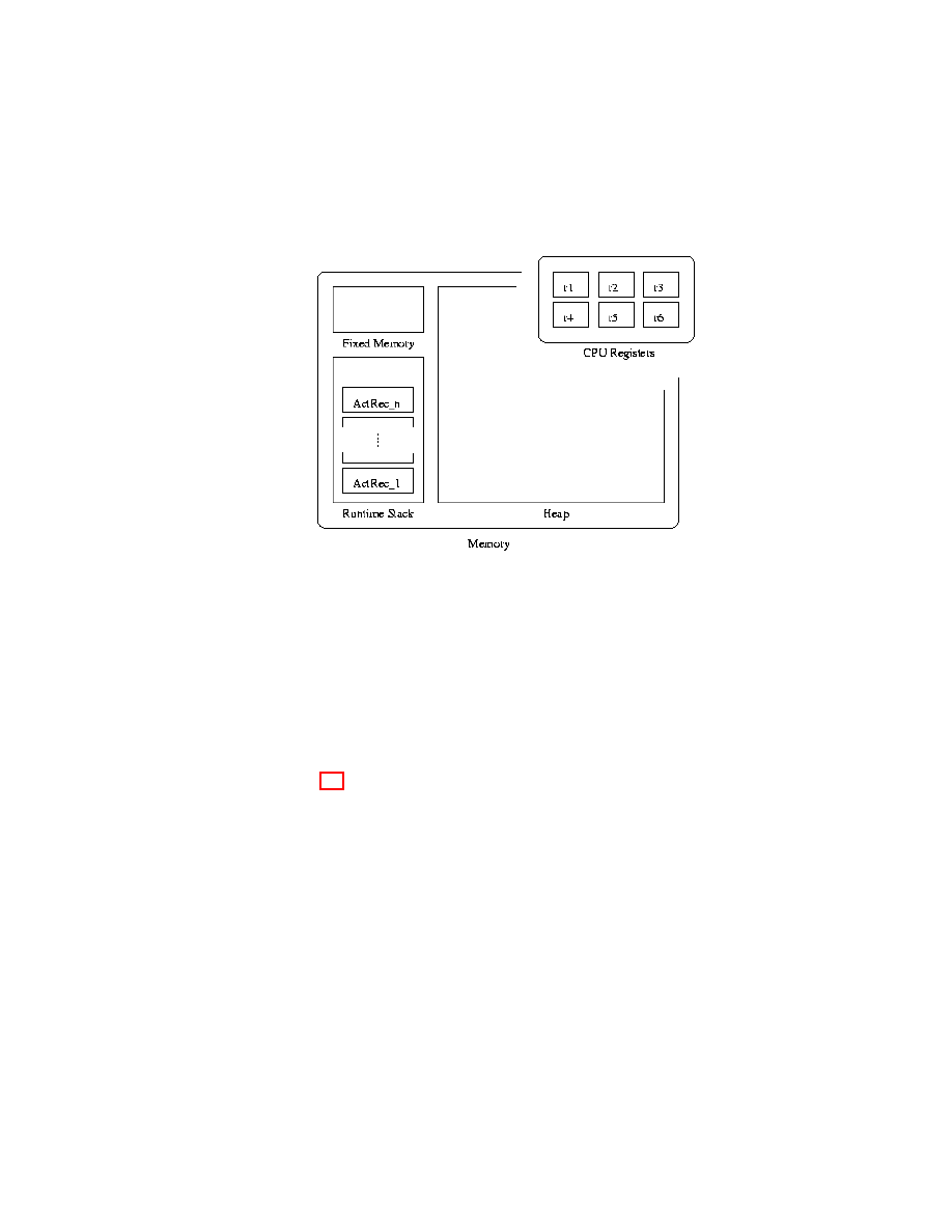
132
CHAPTER 7. COMPILATION BY PROGRAM TRANSFORMATION
Figure 7.1: Our model of memory
Stack-stored entities are also temporary in that they will be junk when the
function/method returns.
Another important issue is whether to box or unbox values.
Definition 7.4. A register or memory location v
i
’s value is stored boxed if v
i
holds a pointer to a block of memory containing the actual value. A variable’s
value is unboxed if it is directly in the register or memory location v
1
.
Figure 7.2 illustrates the difference between boxed and unboxed values.
For multi-word entities such as arrays, storing them unboxed means variables
directly hold a pointer to the first word of the sequence of space. To clarify the
above concepts we review C’s memory layout convention. Variables may be
declared either as globals, register (the register directive is a request to put in
a register only), or on the call stack; all variables declared inside a function
are kept on the stack. Variables directly holding ints, floats, structs, and
arrays are all unboxed. (Examples: int x; float x; int arr[10]; snork x
for snork a struct.) There is no such thing as a variable directly holding a
function; variables in C may only hold pointers to functions. It is possible to
write “v = f” in C where f is a previously declared function and not “v = &f”,
but that is because the former is really syntactic sugar for the latter. A pointer
to a function is in fact a pointer to the start of the code of the function. Boxed
variables in C are declared explicitly, as pointer variables. (Examples: int
*x; float *x; int *arr[10]; snork *x for snork a struct.) All malloc’ed
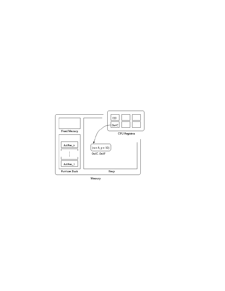
7.4. TRANSLATION TO C
133
Figure 7.2: Boxed vs. unboxed values. The integer value 123 is stored as an
unboxed value, while the record {x=5; y=10} is stored as a boxed value.

134
CHAPTER 7. COMPILATION BY PROGRAM TRANSFORMATION
structures must be stored in a pointer variable because they are boxed: variables
can’t directly be heap entities. Variables are static and the heap is dynamic.
Here is an example of a simple C program and the Sun SPARC assembly
output which gives some impressionistic idea of these concepts:
int glob;
main()
{
int x;
register int reg;
int* mall;
int arr[10];
x = glob + 1;
reg = x;
mall = (int *) malloc(1);
x = *mall;
arr[2] = 4;
/* arr = arr2; --illegal:
arrays are not boxed */
}
In the assembly language, %o1 is a register, [%o0] means dereference, [%fp-24]
means subtract 24 from frame pointer register %fp and dereference. The assem-
bly representation of the above C code is as follows.
main:
sethi
%hi(glob), %o1
or
%o1, %lo(glob), %o0 /* load global address glob into %o0 */
ld
[%o0], %o1
/* dereference */
add
%o1, 1, %o0
/* increment */
st
%o0, [%fp-20] /* store in [%fp-20], 20 back from fp -- x */
/* x directly contains a number,
/* not a pointer */
ld
[%fp-20], %l0 /* %l0 IS reg (its in a register directly) */
mov
1, %o0
call
malloc, 0
/* call malloc.
resulting address to %o0 */
nop
st
%o0, [%fp-24] /* put newspace location in mall [%fp-24] */
ld
[%fp-24], %o0 /* load mall into %o0 */
ld
[%o0], %o1
/* this is a malloced structure -- unbox. */
st
%o1, [%fp-20] /* store into x */
mov
4, %o0
st
%o0, [%fp-56] /* array is a sequence of memory on stack
*/
.LL2:
ret
restore

7.4. TRANSLATION TO C
135
Our memory layout strategy is more like a higher-level language such as
Java or ML. The Java JVM uses a particular, fixed, memory layout scheme:
all object references are boxed pointers to heap locations; the primitive bool,
byte, char, short, int, long, float, and double types are kept unboxed. Since
Java arrays are objects they are also kept boxed. There is no reference (&) or
dereference (*) operator in Java. These operations occur implicitly.
Memory layout for our F[SR compiler
F[SR is (mostly) a Caml subset
and so its memory is also managed more implicitly than C memory. We will
use a simple, uniform scheme in our compilers which is close in spirit to Java’s:
Box Refs and records and function values, but keep boolean values and integers
unboxed. Also, as in C (and Java), all local function variables will be allocated
on the stack and accessed as offsets from the stack pointer. We will achieve the
latter by implementing F[SR local variables as C local variables, which will be
stack allocated by the C compiler.
Since a Ref is nothing but a mutable location, there may not seem to be any
reason to box it. However, if a function returns a Ref as result, and it were not
boxed, it would have been allocated on the stack and thus would be deallocated.
Here is an example that reflects this problem:
Let f = (Function x -> Ref 5) In !f( ) + 1
If Ref 5 were stored on the stack, after the return it could be wiped out.
All of the Let-defined entities in our tuples (the vi variables) can be either in
registers or on the call stack: none of those variables are directly used outside
the function due to lexical scoping, and they don’t directly contain values that
should stay alive after the function returns.
For efficiency, they can all be
declared as register Word variables:
register Word v1, v2, v3, v4, ...;
One other advantage of this simple scheme is every variable holds one word
of data, and thus we don’t need to keep track of how much data a variable is
holding. This scheme is not very efficient, and real compilers optimize signif-
icantly. One example is Ref’s which are known to not escape a function can
unboxed and stack allocated.
All that remains is to come up with a scheme to compile each of the above
atomic tuples and we are done. Records are the most difficult so we will consider
them before writing out the full translation.
Compiling untyped records
Recall from when we covered records that the
fields present in a record cannot be known in advance if there is no type system.
So, we won’t know where the field that we need is exactly. Consider, for example,
(Function x -> x.l)(If y = 0 Then {l = 3} Else {a = 4; l = 3})

136
CHAPTER 7. COMPILATION BY PROGRAM TRANSFORMATION
Field l will be in two different positions in these records so the selection will not
have a sole place it can find the field in. Thus we will need to use a hashtable for
record lookup. In a typed language such as Caml this problem is avoided: the
above code is not well-typed in Caml because the if-then can’t be typed. Note
that the problems with records are closely related to problems with objects,
since objects are simply records with Refs.
This memory layout difficulty with records illustrates an important rela-
tionship between typing and compilation. Type systems impose constraints on
program structure that can make compilers easier to implement. Additionally,
typecheckers will obviate the need to deal with certain run-time errors. Our sim-
ple F[SR compilers are going to core dump on e.g. 4 (5); in Lisp, Smalltalk,
or Scheme these errors would be caught at run-time but would slow down exe-
cution. In a typed language, the compiler would reject the program since it will
not typecheck. Thus for typed languages they will both be faster and safer.
Our method for compilation of records proceeds as follows. We must give
records a heavy implementation, as hash tables (i.e., a set of key-value pairs,
where the keys are label names). In order to make the implementation simple,
records are boxed so they take one word of memory, as mentioned above when
we covered boxing. A record selection operation v
k
.l is implemented by hashing
on key l in the hash table pointed to by v
k
at runtime. This is more or less how
Smalltalk message sends are implemented, since records are similar to objects
(and Smalltalk is untyped).
The above is less than optimal because space will be needed for the hashtable,
and record field accessing will be much slower than, for example, struct access
in C. Since closures are records, this will also significantly slow down function
call. A simple optimization would be to treat closure records specially since the
field positions will always be fixed, and use a struct implementation of closure
(create a different struct type for each function).
For instance, consider
(Function x -> x.l)(If y = 0 Then {l = 3} Else {a = 4; l = 3})
The code x.l will invoke a call of approximate form hashlookup(x,"l"). {a
= 4; l = 3} will create a new hash table and add mappings of "a" to 4 and
"l" to 3.
7.4.2
The toC translation
We are now ready to write the final translation to C, via functions
• toCTuple mapping an atomic tuple to a C statement string,
• toCTuples mapping a list of tuples to C statements,

7.4. TRANSLATION TO C
137
• toCFunction mapping a primitive F[SR function to a string defining a C
function,
• toC mapping a list of primitive F[SR functions to a string of C functions.
The translation as informally written below takes a few liberties for sim-
plicity. Strings "..." below are written in shorthand. For instance "vi = x"
is shorthand for tostring(vi) ^" = " ^tostring(x). The tuples Let x1 =
e1 In Let ...In Let xn = en In xn of function and then/else bodies are as-
sumed to have been converted to lists of tuples [(x1,e1),...,(xn,en)], and
similarly for the list of top-level function definitions. When writing a compiler,
it probably will be easier just to simply keep them in Let form, although either
strategy will work.
toCTuple(vi = x) =
"vi = x;" (* x is a DSR variable *)
toCTuple(vi = n) =
"vi = n;"
toCTuple(vi = b) =
"vi = b;"
toCTuple(vi = vj + vk) =
"vi = vj + vk;"
toCTuple(vi = vj - vk) =
"vi = vj - vk;"
toCTuple(vi = vj And vk ) =
"vi = vj && vk;"
toCTuple(vi = vj Or vk ) =
"vi = vj || vk;"
toCTuple(vi = Not vj ) =
"vi = !vj;"
toCTuple(vi = vj = vk) =
"vi = (vj == vk);"
toCTuple(vi = (vj vk) =
"vi = *vj(vk);"
toCTuple(vi = Ref vj) =
"vi = malloc(WORDSIZE); *vi = vj;"
toCTuple(vi = vj := vk) =
"vi = *vj = vk;"
toCTuple(vi = !vj) =
"vi = *vj;"
toCTuple(vi = { l1 = v1; ... ; ln = vn }) =
/* 1. malloc a new hashtable at vi
2. add mappings l1 -> v1 , ... , ln -> vn
*/
toCTuple(vi = vj.l) =
"vi = hashlookup(vj,"l");"
toCTuple(vi = If vj Then tuples1 Else tuples2) =
"if (vj) { toCTuples(tuples1) } else { toCTuples(tuples2) };"
toCtuples([]) = ""
toCtuples(tuple::tuples) = toCtuple(tuple) ^ toCtuples(tuples)
toCFunction(f = Function xx -> tuples) =
"Word f(Word xx) {" ^ ... declare temporaries ...
toCtuples(tuples) ^
"return(resultId tuples); };"
toCFunctions([]) = ""
toCFunctions(Functiontuple::Functiontuples) =
toCFunction(Functiontuple) ^ toCFunctions(Functiontuples)
(* toC then invokes toCFunctions on its list of functions. *)
The reader may wonder why a fresh memory location is allocated for a Ref,
as opposed to simply storing the existing address of the object being referenced.

138
CHAPTER 7. COMPILATION BY PROGRAM TRANSFORMATION
This is a subtle issue, but the code vi = &vj, for example, would definitely not
work for the Ref case (vj may go out of scope).
This translation sketch above leaves out many details. Here is some elabo-
ration.
Typing issues
We designed out memory layout so that every entity takes up
one word. So, every variable is of some type that is one word in size. Type all
variables as Word’s, where Word is a 1-word type (defined as e.g. typedef void
*Word;). Many type casts need to be inserted; we are basically turning off the
type-checking of C, but there is no ”switch” that can be flicked. So, for instance
vi = vj + vk will really be vi = (Word (int vj) + (int vk)) – cast the
words to ints, do the addition, and cast back to a word. To cast to a function
pointer is a tongue-twister: in C you can use (*((Word (*)()) f))(arg). The
simplest way to avoid confusion when actually writing a compiler is to include
the following typedefs to the resulting C code:
/*
* Define the type ‘Word’ to be a generic one-word value.
*/
typedef void *Word;
/*
* Define the type ‘FPtr’ to be a pointer to a function that
* consumes Word and returns a Word.
All translated
* functions should be of this form.
*/
typedef Word (*FPtr)(Word);
/*
* Here is an example of how to use these typedefs in code.
*/
Word my function(Word w) {
return w;
}
int main(int argc, char **argv) {
Word f1 = (Word) my function;
Word w1 = (Word) 123;
Word w2 = ( *((FPtr) f1) )(w1); /* Computes f1(123) */
printf("%d\n", (int) w2);
/* output is "123\n". */
return 0;
}
Global Issues
Some global issues you will need to deal with include the fol-
lowing. You will need to print out the result returned by the main function (so,
you probably want the DSR main function to be called something like DSRmain

7.5. SUMMARY
139
and then write your own main() by hand which will call DSRmain); The C func-
tions need to declare all the temporary variables they use. One solution is to
declare in the function header a C array
Word v[22]
where 22 is the number of temporaries needed in this particular function, and
use names v[0], v[1], etc for the temporaries. Note, this works well only if
the newid() function is instructed to start numbering temporaries at zero again
upon compiling each new function. Every compiled program is going to have to
come with a standard block of C code in the header, including the record hash
implementation, main() as alluded to above, etc.
Other issues that present problems include the following. Record creation is
only sketched; but there are many C hash set libraries that could be used for this
purpose. The final result (resultId) of the Then and Else tuples needs to be
in the same variable vi, which is also the variable where the result of the tuple
is put, for the If code to be correct. This is best handled in the A-translation
phase.
There are several other issues that will arise when writing the compiler. The
full implementation is left as an exercise.
7.4.3
Compilation to Assembly code
Now that we have covered the compilation to C, we informally consider how a
compiler would compile all the way to machine code. The C code we produce
above is very close to assembly code. It would be conceptually easy to translate
into assembly, but we skip the topic due to the large number of cases that arise
in the process (saving registers, allocating space on the stack for temporaries.
7.5
Summary
let frontend e = hoist(atrans(clconv(e)));;
let translator e = toC(frontend(e));;
We can assert the correctness of our translator.
Theorem 7.4. DSR program e terminates in the F[SR operational semantics
(or evaluator) just when the C program translator(e) terminates, provided the
C program does not run out of memory. Core dump or other run-time errors
are equated with nontermination. Furthermore, if F[SR’s eval(e) returns a
number n, the compiled translator(e) will also produce numerical output n.

140
CHAPTER 7. COMPILATION BY PROGRAM TRANSFORMATION
7.6
Optimization
Optimization can be done at all phases of the translation process. The above
translation is simple, but inefficient. There is always a tradeoff between sim-
plicity and efficiency in compiler designs, both the efficiency of compilation
itself, and efficiency of code produced. In the phases before C code is produced,
optimizations consist of replacing chunks of the program with operationally
equivalent chunks.
Some simple optimizations include the following. The special closure records
{fn = .., envt = ..
} could be implemented as a pointer to a C struct
with fn and envt fields, instead of using the very slow hash method,
will
significantly speed up the code produced. Records which do not not have field
names overlapping with other records can also be implemented in this manner
(there can be two different records with the same fields, but not two different
records with some fields the same and some different). Another optimization is
to modify the A-translation to avoid making tuples for variables and constants.
Constant expressions such as 3 + 4 can be folded to 7.
More fancy optimizations require a global flow analysis be performed. Sim-
ply put, a flow analysis finds all possible uses of a particular definition, and all
possible definitions corresponding to a particular use.
A definition is a record, a Function, or a number or boolean, and a use is a
record field selection, function application, or numerical or boolean operator.
7.7
Garbage Collection
Our compiled code mallocs but never frees. We will eventually run out of
memory. A garbage collector is needed.
Definition: In a run-time image, memory location n is garbage if it never
will be read or written to again.
There are many notions of garbage detection. The most common is to be
somewhat more conservative and take garbage to be memory locations which
are not pointed to by any known (”root”) object.
1
Although hash lookups are O(1), there is still a large amount of constant overhead,
whereas struct access can be done in a single load operation.

Appendix A
DDK: The F[ Development
Kit
The F[ Development Kit, or DDK, is a small set set of utilities for working with
our example languages, F[ and F[SR. DDK is useful in two ways. First, it
provides the binaries F[ and F[SR for toplevel and file-based interpretation. In
addition, all of the source code for DDK is available, except for the interpreters.
The reader may write his own F[ or F[SR interpreter, and plug it into the
DDK source to make a toplevel and file interpreter for testing purposes. This
appendix explains how to use the DDK binaries, and gives an overview of the
source code.
Before we begin, let’s establish a notation for the examples in this appendix.
Shell commands and expressions within the toplevel are typeset in typewriter
font. Lines beginning with “$” are shell commands, while lines beginning with
“#” are expressions typed within the toplevel. Lastly, lines beginning with “==>”
are the resulting values computed by the toplevel.
A.1
Installing the DDK
DDK should run on any platform which supports OCaml and the OCaml de-
velopment tools. It is recommended, although not strictly necessary, that you
compile DDK on a Unix or Unix-like platform which supports GNU Make.
The DDK bytecode binaries are available at
http://www.cs.jhu.edu/~scott/pl/book/DDK/downloads/binaries.
Download the bytecode tar archive ddk-0.1-byte.tar.gz. Make a temporary
directory, and move the archive there and unpack it:
$ mkdir ddk tmp
$ mv ddk-0.1-byte.tar.gz ddk tmp
$ cd ddk tmp
$ gunzip -c ddk-0.1-byte.tar.gz | tar x
141

142
APPENDIX A. DDK: THE F[ DEVELOPMENT KIT
Now there will be a subdirectory with the same name as the tar archive (without
the .tar.gz extension). In this directory are two bytecode files: d.byte and
dsr.byte. Now, simply execute the shell command ocamlrun d.byte to run a
D top loop, and similarly for DSR.
The DDK source is available at
http://www.cs.jhu.edu/~scott/pl/book/DDK/downloads/source
The source requires no installation. Simply unpack the source archive in the
directory of your choice. We will discuss how to work with the source code in
Section A.3.7.
A.2
Using F[ and F[SR
The F[ and F[SR utilities both have similar syntax and functionality,
and so
without loss of generality, we will discuss only F[SR in this section. There are
two ways to use F[SR: as a toplevel, and as a file-based interpreter. If ever in
doubt, type
$ F[SR --help
to see the correct usage.
A.2.1
The Toplevel
The F[SR toplevel is extremely similar to the Caml toplevel, and should seem
quite familiar and intuitive. The toplevel is good for testing small chunks of
code. For anything that is too long to type or paste into the toplevel, F[SR
should be run against a file instead. To run the toplevel, simply type
$ F[SR
To exit the toplevel, press CTRL+C at any time.
Once in the toplevel, the # prompt appears. At the # prompt, any F[SR
expression may be entered, followed by a ;;, just as in Caml. The expression
is evaluated and the value is output after a ==>. For example,
# 3 + 4;;
==> 7
# (Function x -> x + 1) 5;;
==> 6
# True Or False;;
==> True
The toplevel behaves much like the Caml toplevel, but has a few differences.
The main difference is that Let statements must always have an explicit In. This
1
F[ and F[SR are built out of the same functor, parameterized by language.
This will
become clearer after reading Section A.3.

A.3. THE DDK SOURCE CODE
143
means that F[SR programs must be input as one continuous string expression,
and evaluation does not begin until the ;; is input. For this reason, larger
programs should be written as files, and directly interpreted instead of input at
the toplevel.
The second difference is more of an advantage. Unlike the Caml toplevel,
the F[SR toplevel always outputs a full representation of its result values. This
is particular useful for looking at expressions that evaluate to functions. While
Caml just reports the value as <fun>, F[SR gives a full description. For exam-
ple,
# (Function x -> Function y -> Function z -> x + y + z) 4 5;;
==> Function z ->
4 + 5 + z
Notice how we can see the full result of the currying. This is useful for debugging
large functions.
A.2.2
File-Based Intrepretation
In addition to a toplevel, the F[SR utility can also directly intrepret a file. This
is useful for interpreting larger programs that are difficult to enter into the
toplevel. Comments of the form (*. . . *) are valid in F[SR, and can be added to
improve the readability of the code. To interpret a file, simply type
$ F[SR myprogram.dsr
The value result of the program will be displayed on standard output. For
example, interpreting the merge sort example in Section 4.3.2 would look like
this.
$ F[SR mergesort.dsr
{l=1; r={l=2; r={l=3; r={l=4; r={l=5; r={l=6; r=
{l=7; r={l=8; r={l=9; r={l=10; r=-1}}}}}}}}}}
A.3
The DDK Source Code
In this section, we will give an overview of the DDK source code. DDK is
written in Objective Caml 3.07[15]. The main reason to become familiar with
the source code is to learn how to write an interpreter than can “plug in” to
DDK. Plugging in an interpreter builds a toplevel and file-based interpreter over
top of it, and allows the developer to test his interpreter on expressions in the
concrete syntax, which is much easier then trying to write abstract syntax out
by hand. Let’s begin by surveying the major components od the DDK source.
In the following sections, we assume the DDK source code is installed in a
directory called $DDK SRC (this will be the directory that is created when the
source archive is expanded).

144
APPENDIX A. DDK: THE F[ DEVELOPMENT KIT
A.3.1
$DDK SRC/src/ddk.ml
ddk.ml defines the Ddk module.
This module contains a single module signa-
ture type, LANGUAGE. Any module that implements this signature can be used
to create a toplevel of file interpreter.
module type LANGUAGE = sig
val name: string
module Ast: sig
type expr
end
module Parser: sig
type token
val main:
(Lexing.lexbuf -> token) -> Lexing.lexbuf -> Ast.expr
end
module Lexer: sig
val token: Lexing.lexbuf -> Parser.token
end
module Pp: sig
val pretty_print: Ast.expr -> string
val pp: Ast.expr -> string -> string
end
module Interpreter: sig
val eval: Ast.expr -> Ast.expr
end
end;;
A.3.2
$DDK SRC/src/application.ml
The Application module implements the toplevel and file interpreter in a lan-
guage independent way. It contains a functor Make that is parameterized on
Ddk.LANGUAGE. A module with signature Application.S is returned, which
contains a function main. Therefore, a new toplevel and file interpreter can be
trivially written as
2
Recall from the OCaml manual that “[t]he [ocamlc] compiler always derives the module
name by taking the capitalized base name of the source file (.ml or .mli file). That is, it strips
the leading directory name, if any, as well as the .ml or .mli suffix; then, it [sets] the first
letter to uppercase, in order to comply with the requirement that module names must be
capitalized.”[15]

A.3. THE DDK SOURCE CODE
145
module MyApplication = Application.Make(MyLanguage);;
MyApplication.main();;
The code for the Application module is as follows.
module type S =
sig
val main: unit -> unit
end
module Make(Lang: Ddk.LANGUAGE) =
struct
let toplevel_loop () =
Printf.printf "\t%s version %s\n\n"
Lang.name Version.version;
flush stdout;
while true do
Printf.printf "# ";
flush stdout;
let lexbuf = Lexing.from_channel stdin in
let ast = Lang.Parser.main Lang.Lexer.token lexbuf in
let result = Lang.Interpreter.eval ast in
Printf.printf "==> %s\n" (Lang.Pp.pp result "
");
flush stdout
done
let run_file filename =
let fin = open_in filename in
let lexbuf = Lexing.from_channel fin in
let ast = Lang.Parser.main Lang.Lexer.token lexbuf in
let result = Lang.Interpreter.eval ast in
Printf.printf "%s\n" (Lang.Pp.pretty_print result);
flush stdout
let print_version () =
Printf.printf "%s version %s\nBuild Date: %s\n"
Lang.name Version.version Version.date
let main () =
let filename = ref "" in
let toplevel = ref true in
let version = ref false in
Arg.parse
[("--version",

146
APPENDIX A. DDK: THE F[ DEVELOPMENT KIT
Arg.Set(version),
"show version information")]
(function fname ->
filename := fname;
version := false;
toplevel := false)
("Usage: " ^
Lang.name ^
" [ options ] [ filename ]\noptions:");
if !version then
print_version ()
else if !toplevel then
toplevel_loop ()
else
run_file !filename
end
A.3.3
$DDK SRC/src/D/d.ml
The codebases for F[ and F[SR are, for the most part, parallel, therefore we will
examine only the F[ code, and not F[SR. The D module is an implementation
of Ddk.LANGUAGE and is very straightforward.
module Language = struct
let name = "D"
module Parser = Dparser
module Lexer = Dlexer
module Ast = Dast
module Pp = Dpp
module Interpreter = Dinterp
end;;
module Application = Application.Make(Language);;
Application.main ();;
A.3.4
$DDK SRC/src/D/dast.ml
The Dast module contains a type expr that is the type of the abstract syntax
tree for our language. It is exactly as we defined it in Section 2.3.
type ident = Ident of string

A.3. THE DDK SOURCE CODE
147
type expr =
Var of ident | Function of ident * expr | Appl of expr * expr |
Letrec of ident * ident * expr * expr |
Plus of expr * expr | Minus of expr * expr | Equal of expr * expr |
And of expr * expr| Or of expr * expr | Not of expr |
If of expr * expr * expr | Int of int | Bool of bool
A.3.5
$DDK SRC/src/D/dpp.ml
Dpp is a pretty-printer for F[. The function pretty print takes a Dast.expr
and returns a string representation in the concrete syntax. In other words, it
converts from abstract to concrete syntax. This is used to display the result of
a computation.
open Dast;;
let rec pp e pad =
match e with
Bool(true) -> "True"
| Bool(false) -> "False"
| Int(x) -> string_of_int x
| Plus(e1, e2) ->
pp e1 pad ^ " + " ^ pp e2 pad
| Minus(e1, e2) ->
pp e1 pad ^ " - " ^ pp e2 pad
| Equal(e1, e2) ->
pp e1 pad ^ " = " ^ pp e2 pad
| And(e1, e2) ->
pp e1 pad ^ " And " ^ pp e2 pad
| Or(e1, e2) ->
pp e1 pad ^ " Or " ^ pp e2 pad
| Not(e1) ->
"Not " ^ pp e1 pad
| Appl(e1, e2) ->
"(" ^ pp e1 pad ^ ") (" ^ pp e2 pad ^ ")"
| Var(Ident(x)) -> x
| Function(Ident(i), x) ->
let newpad = pad ^ "
" in
"Function " ^ i ^ " ->\n" ^ newpad ^ pp x newpad
| If(e1, e2, e3) ->
let newpad = pad ^ "
" in
"If " ^ pp e1 pad ^ " Then\n" ^ newpad ^ pp e2 newpad ^
"\n" ^ pad ^ "Else\n" ^ newpad ^ pp e3 newpad
| Letrec(Ident(i1), Ident(i2), e1, e2) ->
let newpad = pad ^ "
" in

148
APPENDIX A. DDK: THE F[ DEVELOPMENT KIT
"Let Rec " ^ i1 ^ " " ^ i2 ^ " =\n" ^ newpad ^
pp e1 newpad ^ "\n" ^ pad ^ "In\n" ^ newpad ^
pp e2 newpad
let pretty_print e = (pp e "") ^ "\n"
A.3.6
Scanning and Parsing Concrete Syntax
The scanner and parser are written using the parser generation tools ocamlyacc
and ocamllex, which are similar to the C-based yacc and lex tools. Using such
tools is beyond the scope of this book, but the interested reader is directed to the
source files $DDK SRC/src/D/dlexer.mly and $DDK SRC/src/D/dparser.mly
for the scanner and parser sources respectively.
A.3.7
Writing an Interpreter
The source distribution already contains a “template” for both the F[ and
F[SR interpreters. For example, the file $DDK SRC/src/D/dinterp.ml con-
tains a dummy implementation of Ddk.LANGUAGE.Intreperter in which eval e
simply returns e. $DDK SRC/src/DSR/dsrinterp.ml contains a similar dummy
inplementation for F[SR. Simply replace the dummy definition of eval with
the code for a real interpreter, and rebuild DDK (building DDK is discussed
in the next section). Note that supporting functions may and should be used
when writing eval. As long as eval is defined, the interpreter will conform to
the signature regardless of other functions that are defined.
As a reference point, the directory $DDK SRC/src/BOOL contains a full imple-
mentation of the boolean toplevel and interpreter. The implementation mirrors
the F[ implementation that we looked at above.
Building DDK
The final point we need to discuss is how to actually build DDK. Luckily, doing
so is very straightforward. Before building for the first time, you will need to
configure the build process for your platform. This is done by going to the
$DDK SRC directory and typing
$ ./configure
The configure script checks for the OCaml tools that are needed to build
the source, and also determines whether to use a native compiler, or whether
to compile to bytecode. Note that the directory containing ocaml, ocamlc,
ocamlyacc, etc. should be in your path before running the configure script.
Once the configure script is finished, you should see a Makefile in the
$DDK SRC directory. Once the Makefile is there, configure does not need to
be run again, unless you move the source to a different platform.

A.3. THE DDK SOURCE CODE
149
Now, DDK can be built at any time by going to the $DDK SRC directory and
typing
$ make
make will build the binaries F[, F[SR, and BOOL and copy them to the $DDK SRC
directory, from where then can be run, for example, as
$ ./F[SR
If you platform does not support sh and GNU Make, you can still build
DDK. Windows users should use win32Build.bat to build DDK. Note that
you can comment out the lines of this file that you don’t need, it builds all three
interpreters.
Suggested Strategy for Writing the Interpreters
The best strategy for writing the interpreter is probably to add a single clause
at a time to the eval function, and then to rebuild and test that clause. Let’s
walk through an example. Assuming the configure script has already been run,
build DDK without modifying the dummy interpreter by typing make.
Now run the F[ toplevel by typing
$ ./F[
Try entering in an expression into the toplevel. The dummy interpreter simply
spits the expression back without evaluating it, so your session will look like
# 3+4;;
==> 3 + 4
Press CTRL+C to exit the toplevel. Now let’s write the match case for addition.
Open the file $DDK SRC/src/D/dinterp.ml in your favorite text editor. The
file should initially look as follows.
open Dast;;
(*
* Replace this with your interpreter code.
*)
let rec eval e = e
Make the following modifications to dinterp.ml.
open Dast;;
exception TypeMismatch;;
exception NotImplemented;;

150
APPENDIX A. DDK: THE F[ DEVELOPMENT KIT
(*
* Replace this with your interpreter code.
*)
let rec eval e =
match e with
Int x -> Int x
| Plus(e1, e2) ->
(match (eval e1, eval e2) with
(Int(x), Int(y)) -> Int(x + y)
| _ -> raise TypeMismatch)
| _ -> raise NotImplemented
Now, rebuild DDK by typing make in the $DDK SRC directory again. Run
the F[ toplevel. Now, we can evaluate addition expressions:
# 3+4;;
==> 7
Proceed in this manner, adding one or two match cases, and then testing,
then adding some more match cases. This way, if an error occurs, it will be easy
to figure out which changes caused it.

Appendix B
GNU Free Documentation
License
Version 1.1, March 2000
Copyright c
2000 Free Software Foundation, Inc.
59 Temple Place, Suite 330, Boston, MA 02111-1307 USA
Everyone is permitted to copy and distribute verbatim
copies of this license document, but changing it is not
allowed.
Preamble
The purpose of this License is to make a manual, text-
book, or other written document “free” in the sense of
freedom:
to assure everyone the effective freedom to
copy and redistribute it, with or without modifying it,
either commercially or noncommercially.
Secondarily,
this License preserves for the author and publisher a way
to get credit for their work, while not being considered
responsible for modifications made by others.
This License is a kind of “copyleft”, which means
that derivative works of the document must themselves
be free in the same sense. It complements the GNU Gen-
eral Public License, which is a copyleft license designed
for free software.
We have designed this License in order to use it for
manuals for free software, because free software needs
free documentation:
a free program should come with
manuals providing the same freedoms that the software
does. But this License is not limited to software man-
uals; it can be used for any textual work, regardless of
subject matter or whether it is published as a printed
book. We recommend this License principally for works
whose purpose is instruction or reference.
Applicability and Definitions
This License applies to any manual or other work that
contains a notice placed by the copyright holder saying
it can be distributed under the terms of this License.
The “Document”, below, refers to any such manual or
work.
Any member of the public is a licensee, and is
addressed as “you”.
A “Modified Version” of the Document means any
work containing the Document or a portion of it, either
copied verbatim, or with modifications and/or trans-
lated into another language.
A “Secondary Section” is a named appendix or a
front-matter section of the Document that deals exclu-
sively with the relationship of the publishers or authors
of the Document to the Document’s overall subject (or
to related matters) and contains nothing that could fall
directly within that overall subject. (For example, if the
Document is in part a textbook of mathematics, a Sec-
ondary Section may not explain any mathematics.) The
relationship could be a matter of historical connection
with the subject or with related matters, or of legal,
commercial, philosophical, ethical or political position
regarding them.
The “Invariant Sections” are certain Secondary Sec-
tions whose titles are designated, as being those of In-
variant Sections, in the notice that says that the Docu-
ment is released under this License.
The “Cover Texts” are certain short passages of
text that are listed, as Front-Cover Texts or Back-Cover
Texts, in the notice that says that the Document is re-
leased under this License.
A “Transparent” copy of the Document means a
machine-readable copy, represented in a format whose
specification is available to the general public, whose
contents can be viewed and edited directly and straight-
forwardly with generic text editors or (for images com-
posed of pixels) generic paint programs or (for drawings)
some widely available drawing editor, and that is suit-
able for input to text formatters or for automatic trans-
lation to a variety of formats suitable for input to text
formatters.
A copy made in an otherwise Transparent
file format whose markup has been designed to thwart
or discourage subsequent modification by readers is not
Transparent. A copy that is not “Transparent” is called
“Opaque”.
Examples of suitable formats for Transparent copies
include plain ASCII without markup, Texinfo input for-
mat, L
ATEX input format, SGML or XML using a pub-
licly available DTD, and standard-conforming simple HTML
designed for human modification.
Opaque formats in-
clude PostScript, PDF, proprietary formats that can be
read and edited only by proprietary word processors,
SGML or XML for which the DTD and/or processing
tools are not generally available, and the machine-generated
HTML produced by some word processors for output
purposes only.
The “Title Page” means, for a printed book, the
title page itself, plus such following pages as are needed
to hold, legibly, the material this License requires to ap-
pear in the title page.
For works in formats which do
not have any title page as such, “Title Page” means the
text near the most prominent appearance of the work’s
title, preceding the beginning of the body of the text.
Verbatim Copying
You may copy and distribute the Document in any medium,
either commercially or noncommercially, provided that
this License, the copyright notices, and the license no-
tice saying this License applies to the Document are re-
produced in all copies, and that you add no other condi-
tions whatsoever to those of this License. You may not
use technical measures to obstruct or control the reading
or further copying of the copies you make or distribute.
However, you may accept compensation in exchange for
copies. If you distribute a large enough number of copies
you must also follow the conditions in section 3.
You may also lend copies, under the same condi-
tions stated above, and you may publicly display copies.
151

152
APPENDIX B. GNU FREE DOCUMENTATION LICENSE
Copying in Quantity
If you publish printed copies of the Document number-
ing more than 100, and the Document’s license notice
requires Cover Texts, you must enclose the copies in cov-
ers that carry, clearly and legibly, all these Cover Texts:
Front-Cover Texts on the front cover, and Back-Cover
Texts on the back cover. Both covers must also clearly
and legibly identify you as the publisher of these copies.
The front cover must present the full title with all words
of the title equally prominent and visible. You may add
other material on the covers in addition. Copying with
changes limited to the covers, as long as they preserve
the title of the Document and satisfy these conditions,
can be treated as verbatim copying in other respects.
If the required texts for either cover are too volu-
minous to fit legibly, you should put the first ones listed
(as many as fit reasonably) on the actual cover, and con-
tinue the rest onto adjacent pages.
If you publish or distribute Opaque copies of the
Document numbering more than 100, you must either
include a machine-readable Transparent copy along with
each Opaque copy, or state in or with each Opaque copy
a publicly-accessible computer-network location contain-
ing a complete Transparent copy of the Document, free
of added material, which the general network-using pub-
lic has access to download anonymously at no charge us-
ing public-standard network protocols.
If you use the
latter option, you must take reasonably prudent steps,
when you begin distribution of Opaque copies in quan-
tity, to ensure that this Transparent copy will remain
thus accessible at the stated location until at least one
year after the last time you distribute an Opaque copy
(directly or through your agents or retailers) of that edi-
tion to the public.
It is requested, but not required, that you contact
the authors of the Document well before redistributing
any large number of copies, to give them a chance to
provide you with an updated version of the Document.
Modifications
You may copy and distribute a Modified Version of the
Document under the conditions of sections 2 and 3 above,
provided that you release the Modified Version under
precisely this License, with the Modified Version filling
the role of the Document, thus licensing distribution and
modification of the Modified Version to whoever pos-
sesses a copy of it. In addition, you must do these things
in the Modified Version:
•
Use in the Title Page (and on the covers, if any)
a title distinct from that of the Document, and
from those of previous versions (which should, if
there were any, be listed in the History section
of the Document). You may use the same title
as a previous version if the original publisher of
that version gives permission.
•
List on the Title Page, as authors, one or more
persons or entities responsible for authorship of
the modifications in the Modified Version, to-
gether with at least five of the principal authors
of the Document (all of its principal authors, if
it has less than five).
•
State on the Title page the name of the pub-
lisher of the Modified Version, as the publisher.
•
Preserve all the copyright notices of the Docu-
ment.
•
Add an appropriate copyright notice for your
modifications adjacent to the other copyright
notices.
•
Include, immediately after the copyright notices,
a license notice giving the public permission to
use the Modified Version under the terms of this
License, in the form shown in the Addendum be-
low.
•
Preserve in that license notice the full lists of In-
variant Sections and required Cover Texts given
in the Document’s license notice.
•
Include an unaltered copy of this License.
•
Preserve the section entitled “History”, and its
title, and add to it an item stating at least the
title, year, new authors, and publisher of the
Modified Version as given on the Title Page.
If there is no section entitled “History” in the
Document, create one stating the title, year, au-
thors, and publisher of the Document as given
on its Title Page, then add an item describing
the Modified Version as stated in the previous
sentence.
•
Preserve the network location, if any, given in
the Document for public access to a Transpar-
ent copy of the Document, and likewise the net-
work locations given in the Document for pre-
vious versions it was based on.
These may be
placed in the “History” section. You may omit
a network location for a work that was published
at least four years before the Document itself, or
if the original publisher of the version it refers
to gives permission.
•
In any section entitled “Acknowledgements” or
“Dedications”, preserve the section’s title, and
preserve in the section all the substance and
tone of each of the contributor acknowledgements
and/or dedications given therein.
•
Preserve all the Invariant Sections of the Docu-
ment, unaltered in their text and in their titles.
Section numbers or the equivalent are not con-
sidered part of the section titles.
•
Delete any section entitled “Endorsements”. Such
a section may not be included in the Modified
Version.
•
Do not retitle any existing section as “Endorse-
ments” or to conflict in title with any Invariant
Section.
If the Modified Version includes new front-matter
sections or appendices that qualify as Secondary Sec-
tions and contain no material copied from the Docu-
ment, you may at your option designate some or all of
these sections as invariant. To do this, add their titles to
the list of Invariant Sections in the Modified Version’s
license notice.
These titles must be distinct from any
other section titles.
You may add a section entitled “Endorsements”,
provided it contains nothing but endorsements of your
Modified Version by various parties – for example, state-
ments of peer review or that the text has been approved
by an organization as the authoritative definition of a
standard.
You may add a passage of up to five words as a
Front-Cover Text, and a passage of up to 25 words as a
Back-Cover Text, to the end of the list of Cover Texts
in the Modified Version.
Only one passage of Front-
Cover Text and one of Back-Cover Text may be added
by (or through arrangements made by) any one entity.
If the Document already includes a cover text for the
same cover, previously added by you or by arrangement
made by the same entity you are acting on behalf of, you
may not add another; but you may replace the old one,
on explicit permission from the previous publisher that
added the old one.
The author(s) and publisher(s) of the Document do
not by this License give permission to use their names
for publicity for or to assert or imply endorsement of any
Modified Version.
Combining Documents
You may combine the Document with other documents
released under this License, under the terms defined in
section 4 above for modified versions, provided that you
include in the combination all of the Invariant Sections
of all of the original documents, unmodified, and list
them all as Invariant Sections of your combined work in
its license notice.
The combined work need only contain one copy of
this License, and multiple identical Invariant Sections
may be replaced with a single copy. If there are multi-
ple Invariant Sections with the same name but different
contents, make the title of each such section unique by
adding at the end of it, in parentheses, the name of the
original author or publisher of that section if known, or

153
else a unique number. Make the same adjustment to the
section titles in the list of Invariant Sections in the li-
cense notice of the combined work.
In the combination, you must combine any sections
entitled “History” in the various original documents, form-
ing one section entitled “History”; likewise combine any
sections entitled “Acknowledgements”, and any sections
entitled “Dedications”. You must delete all sections en-
titled “Endorsements.”
Collections of Documents
You may make a collection consisting of the Document
and other documents released under this License, and
replace the individual copies of this License in the vari-
ous documents with a single copy that is included in the
collection, provided that you follow the rules of this Li-
cense for verbatim copying of each of the documents in
all other respects.
You may extract a single document from such a col-
lection, and distribute it individually under this License,
provided you insert a copy of this License into the ex-
tracted document, and follow this License in all other
respects regarding verbatim copying of that document.
Aggregation With Independent Works
A compilation of the Document or its derivatives with
other separate and independent documents or works, in
or on a volume of a storage or distribution medium, does
not as a whole count as a Modified Version of the Doc-
ument, provided no compilation copyright is claimed for
the compilation.
Such a compilation is called an “ag-
gregate”, and this License does not apply to the other
self-contained works thus compiled with the Document,
on account of their being thus compiled, if they are not
themselves derivative works of the Document.
If the Cover Text requirement of section 3 is appli-
cable to these copies of the Document, then if the Doc-
ument is less than one quarter of the entire aggregate,
the Document’s Cover Texts may be placed on covers
that surround only the Document within the aggregate.
Otherwise they must appear on covers around the whole
aggregate.
Translation
Translation is considered a kind of modification, so you
may distribute translations of the Document under the
terms of section 4.
Replacing Invariant Sections with
translations requires special permission from their copy-
right holders, but you may include translations of some
or all Invariant Sections in addition to the original ver-
sions of these Invariant Sections.
You may include a
translation of this License provided that you also include
the original English version of this License.
In case of
a disagreement between the translation and the origi-
nal English version of this License, the original English
version will prevail.
Termination
You may not copy, modify, sublicense, or distribute the
Document except as expressly provided for under this
License. Any other attempt to copy, modify, sublicense
or distribute the Document is void, and will automati-
cally terminate your rights under this License. However,
parties who have received copies, or rights, from you un-
der this License will not have their licenses terminated
so long as such parties remain in full compliance.
Future Revisions of This License
The Free Software Foundation may publish new, revised
versions of the GNU Free Documentation License from
time to time. Such new versions will be similar in spirit
to the present version, but may differ in detail to address
new problems or concerns. See http://www.gnu.org/copyleft/.
Each version of the License is given a distinguishing
version number.
If the Document specifies that a par-
ticular numbered version of this License ”or any later
version” applies to it, you have the option of following
the terms and conditions either of that specified version
or of any later version that has been published (not as a
draft) by the Free Software Foundation. If the Document
does not specify a version number of this License, you
may choose any version ever published (not as a draft)
by the Free Software Foundation.
ADDENDUM: How to use this Li-
cense for your documents
To use this License in a document you have written, in-
clude a copy of the License in the document and put
the following copyright and license notices just after the
title page:
Copyright c
YEAR YOUR NAME. Per-
mission is granted to copy, distribute
and/or modify this document under the
terms of the GNU Free Documentation
License, Version 1.1 or any later version
published by the Free Software Founda-
tion; with the Invariant Sections being
LIST THEIR TITLES, with the Front-
Cover Texts being LIST, and with the
Back-Cover Texts being LIST. A copy
of the license is included in the section
entitled “GNU Free Documentation Li-
cense”.
If you have no Invariant Sections, write “with no
Invariant Sections” instead of saying which ones are in-
variant.
If you have no Front-Cover Texts, write “no
Front-Cover Texts” instead of “Front-Cover Texts being
LIST”; likewise for Back-Cover Texts.
If your document contains nontrivial examples of
program code, we recommend releasing these examples
in parallel under your choice of free software license,
such as the GNU General Public License, to permit their
use in free software.

154
APPENDIX B. GNU FREE DOCUMENTATION LICENSE

Bibliography
[1] The Self programming language.
[2] Typed assembly language. http://www.cs.cornell.edu/talc/.
[3] A.V. Aho, R. Sethi, and J.D. Ullman. Compilers: Principles, Techniques
and Tools. Addison-Wesley, 1986.
[4] A. Appel. Compiling with Continuations. Cambridge University Press,
1992.
[5] Andrew Appel. Modern Compiler Implementation in ML. Cambridge Uni-
versity Press, 1998.
[6] Richard Bird. Introduction to Functional Programming using Haskell. Pren-
tice Hall, 2nd edition, 1998.
[7] Gibblad Bracha and David Griswold. Strongtalk: Typechecking Smalltalk
in a Production Environment. In Proceedings of the OOPSLA ’93 Con-
ference on Object-oriented Programming Systems, Languages and Applica-
tions, pages 215–230, 1993.
[8] Kim Bruce. Foundations of Object-Oriented Languages: Types and Seman-
tics. MIT Press, 2002.
[9] Jonathan Eifrig, Scott Smith, Valery Trifonov, and Amy Zwarico. Appli-
cation of OOP type theory: State, decidability, integration. In OOPSLA
’94, pages 16–30, 1994.
[10] Martin Fowler. UML Distilled. Addison Wesley, 2nd edition, 2000.
[11] Erich Gamma, Richard Helm, Ralph Johnson, and John Vlissides. Design
Patterns: Elements of Reusable Object-Oriented Software. Addison-Wesley
Professional Computing Series. Addison-Wesley, 1994.
[12] Jason Hickey.
Introduction to objective caml, 2001.
caltech.edu/courses/cs134/cs134b/book.pdf.
155

156
BIBLIOGRAPHY
[13] Paul Hudak, John Peterson, and Joseph Fasel. A gentle introduction to
Haskell, version 98, June 2000. http://www.haskell.org/tutorial/.
[14] Andrew D. Irvine. Russell’s paradox. Stanford Encyclopedia of Philosophy,
June 2001. http://plato.stanford.edu/entries/russell-paradox/.
[15] Xavier Leroy. The Objective Caml system release 3.04, documentation and
user’s manual, December 2001. http://caml.inria.fr/ocaml/htmlman.
[16] Ian A. Mason, Scott F. Smith, and Carolyn L. Talcott. From operational
semantics to domain theory. Information and Computation, 128(1):26–47,
1996.
[17] Greg Morrisett, Karl Crary, Neal Glew, Dan Grossman, Richard Samuels,
Frederick Smith, David Walker, Stephanie Weirich, and Steve Zdancewic.
Talx86: A realistic typed assembly language. In 1999 ACM SIGPLAN
Workshop on Compiler Support for System Software, pages 25–35, Atlanta,
GA, USA, May 1999.
[18] J
J
O’Connor
and
E
F
Robertson.
Gottfried
Wilhelm
von
Leibniz.
The
MacTutor
History
of
Mathematics
Archive,
Oc-
tober 1998.
http://www-history.mcs.st-andrews.ac.uk/history/
[19] Randall B. Smith and David Ungar. Self: The power of simplicity. In
Conference proceedings on Object-oriented programming systems, languages
and applications, pages 227–242. ACM Press, 1987.
[20] Randall B. Smith and David Ungar. Programming as an experience: The
inspiration for Self. Lecture Notes in Computer Science, 952:303–??, 1995.
[21] Scott Smith. Programming languages course. http://www.cs/jhu.edu/
[22] J. Stoy. Denotational Semantics: The Scott-Strachey Approach to Program-
ming Language Theory. MIT Press, 1977.
[23] Paul R. Wilson. Uniprocessor garbage collection techniques. ACM Comput-
ing Surveys, 2002. ftp://ftp.cs.utexas.edu/pub/garbage/bigsurv.ps.
Index
A-translation, 124–128
abstract syntax, 7, 11
α-equivalence, 31
atomic tuples, 130
axiomatic semantics, 5
β-equivalence, see also β-reduction,
β-reduction, 33
bound occurrence, see occurrence,
bound
boxed values, 132
call-by-name, 17, 28
call-by-need, 28
call-by-reference, 17
call-by-value, 17
capture, 22, 32
capture-avoiding substitution, 32–33
classes, 77
closed expression, 15
closure, 56
closure conversion, 120–124
compilation, 119–140
concrete syntax, 7, 11
congruence, 31
control operations, 61
curried function, 23
cyclical store, 52–53
DDK, 141–150
source code, 143–150
usage, 142–143
denotational semantics, 5
deterministic languages, 9, 20
dispatch, 75
domain theory, 30
dynamic dispatch, 79–80
environment-based interpreters, see
interpreters, environment-
based
equational inference, 108
equational types, see types, equa-
tional
equivalence, see operational equiva-
lence
η-conversion, 28
η-equivalence, 31
exceptions, 61–67
explicit environment interpreter, 55
faithful implementation, 9, 49
flow analysis, 140
freezing, see also thawing, 24
function hoisting, 128–129
garbage collection, 52, 54–55
generic types, 107
Haskell, 28
information hiding, 75–77
inheritance, 77–79
interpreters
environment-based, 55–56
writing using DDK, 148–150
l-value, see also r-value, 54
lambda-calculus, 32–33
lazy evaluation, 28
logical combinators, 21
loops, 52
metacircular interpreter, 10
157
158
INDEX
metavariables, 5
nonlocal variable, 120
normalizing languages, 9, 20, 98
object polymorphism, 38, 74–75
relation to record polymorphism,
objects, 69–88
encoding as records, 36
occurrence, 14
operational equivalence, 28–33
operational semantics, 4–33
definition, 5
pairs, see tuples
parametric polymorphism, 107
partial recursive function, 11
polymorphism, 37–38
on objects, see object polymor-
phism
on records, see record polymor-
phism
primitive objects, 81
principal type, 107
program context, 29
proof, 8
proof system, 8
r-value, see also l-value, 54
record polymorphism, 37–38
records, 36–40
reflexivity, 30
renaming substitution, see capture-
avoiding substitution
Return, 62–64
runtime environment, 55
Russell’s Paradox, 24–26
self-application encoding, 73
semantics, 5
sequencing, 52
side-effects, 18, 45–67
state, 45–61
static fields, 80–81
static methods, 80–81
store, 47
stuck state, 98
subtype polymorphism, 38
subtyping, 103–107
symmetry, 31
syntax, 5
syntax tree, 11
thawing, see also freezing, 24
threading, 48
transitivity, 31
tuples, 35–36
Turing-complete, 11, 32, 62
tying the knot, 53
type assertion, 95
type checking, 94, 98–99
type environment, 95
type inference, 93, 94, 107–118
and polymorphism, 107–108
constrained, 115–118
type schema, 114
type soundness, 98
type systems, 94–95
dynamic, 91
equational, 108–115
overview of, 90–93
static, 91
checking, see type checking
inference, see type inference
untyped languages, 92
variable capture, see capture
variable substitution, 13–16
definition, 15
variants, 40–43
polymorphism, 40
Document Outline
- Preface
- Introduction
- Operational Semantics
- Tuples, Records, and Variants
- Side Effects: State and Exceptions
- Object-Oriented Language Features
- Type Systems
- Compilation by Program Transformation
- DDK: The F Development Kit
- GNU Free Documentation License
- Bibliography
- Index
Wyszukiwarka
Podobne podstrony:
Easy Rob Program Language
Generics in the Java Programming Language
Sun Java Training SL 275 Java Programming Language Overheads (Sun Microsystems, 2000)
Programming Languages
Classroom types Programs and programming languages
Prentice Hall Linux Assembly Language Programming
EASY ROB Program Command Language
8080 8085 Assembly Language Programming (1977)(Intel)(Pdf)
Prentice Hall Linux Assembly Language Programming
8080 8085 Assembly Language Programming (1977)(Intel)(Pdf)
Ross Jeffries Nlp Flash Cards Hypnotic Language Patterns (Flashcards Bandler Nlp Neuro Linguistic P
Robert Britton Mips Assembly Language Programming 2003 Prentice Hall
Nowy Prezentacja programu Microsoft PowerPoint 5
więcej podobnych podstron