355

R. Przybylak et al. (eds.), The Polish Climate in the European Context:
An Historical Overview

, DOI 10.1007/978-90-481-3167-9_16,

© Springer Science + Business Media B.V. 2010

16.1 Stating the Problem

There have been hundreds of works written on the changes in the air temperature
over Poland and neighboring countries. These changes, at least, during instrumental
observations are well known. The literature dealing with the changes in sea surface
temperature of the Baltic Sea is relatively poor. Soskin

(1963)

analyses the changes

in sea surface temperature (SST) in the period 1900–1950 and notes in the 20s–30s
of the twentieth century the increase in temperature in relation to the preceding
period. Betin and Preobraženskij

(1962)

while dealing with the severe character of

winters in Europe refer to a series of information about the presence of ice cover in
the Baltic Sea and its duration (tenth–eighteenth centuries). This, in an indirect way,
gives some information regarding many centuries’ changes in winter water tem-
perature. These data however, are not continuous as they base on historic docu-
ments (chronicles, diaries, and harbour, merchant and customs documents) and
enable to derive only very general conclusions, regarding changes in the tempera-
ture of waters of the Baltic Sea, limited solely to winter periods.

Numerous remarks about changes in SST over short periods and in small sea

areas can be found in works dealing with biological oceanography and ecology of
the Baltic Sea; they concern different periods after the 1960s. Even, the impressive
in size, hydro meteorological monograph of the Baltic Sea (Terziev et al.

1992)

,

except for a map illustrating distribution of SST, does not deal with many-year
changes in SST. Some Polish monographs on coastal climate or on Polish coastal
zone mention changes in SST (e.g. Mi

ętus et al.

2004)

in the off shore area.

Systematic measures of water temperature at measuring points of IMGW,

1

which in

A.A. Marsz and A. Styszy

ńska

Department of Meteorology and Nautical Oceanography, Gdynia Maritime University,
S

ędzickiego 19, 81-374, Gdynia Nautical

e-mail: [e-mail]
e-mail: [e-mail]

Chapter 16

Changes in Sea Surface Temperature

of the South Baltic Sea (1854–2005)

Andrzej A. Marsz and Anna Styszy

ńska

1

Institute of Meteorology and Water Management in Poland.

356

A.A. Marsz and A. Styszy

ńska

most cases are located in port waters and the very reading is done close to the shore
or in a distance of a few meters from the shore, provide the data.

In 2003 the authors (Marsz and Styszy

ńska

2003)

making use of the data from

COADS

2

presented changes in SST in the sea area covering the Gda

ńsk Bay and

the Gda

ńsk Deep in the years 1871–1992. They stated that there is statistically

significant positive trend in SST in this sea area (+0.009°C year

−1

, p < 0.005) and

strong correlation between changes in SST and the character of winter atmospheric
circulation observed in the examined period. Zblewski

(2006)

carried out a detailed

analysis of changes in SST in the whole Baltic Sea in the period 1982–2002, in
which very strong increase in air temperature was observed over the Baltic Sea and
in regions adjacent to the Baltic Sea. The aim of this work was to find out how the
strong warming of the atmosphere influences SST. The author noted that strong
positive trends, in most cases are statistically significant and what is more, indicate
clear seasonal variability in space almost in the entire surface of the Baltic Sea. The
annual trends in SST defined by Zblewski turned out to be much stronger than those
noted by the authors in the many- year period 1971–1992. Siegel et al.

(2006)

ana-

lyzed changes in SST of the Baltic Sea from Arkona Deep to the end of the Bothnia
Bay over the period 1990–2004. The conclusions they have arrived at, are, to a great
extent, similar to the results obtained by Zblewski

(2006)

.

The most recent works on changes in SST in the Baltic Sea were published in 2008.

Assessment of Climate Change for the Baltic Sea Basin

(2008

; later referred as

ACCBSB) presents the results of modeling of changes in heat amount in the Baltic Sea
and its regions which were observed in 1958–2005 and 1970–2005. As it can be seen
in the results presented by ACCBSB (2008; Fig. 2.49) a visible increase in the heat
amount in the Baltic took place in 1958–2005. Hansson and Omstedt

(2008)

basing on

the data from the twentieth century reconstructed the SST course and Maximum Ice
Extent (MIE) for the last 500 years. The above mentioned results indicate that in the
twentieth century SST was higher than in the last 500-year period and that the highest
decadal values of SST were observed in the 1930s and in the 1730s. The changes in
SST and MIE in the Baltic are within the limits of natural climate variability.

Changes in SST in open waters of the Baltic Sea,

3

because of the presence of a

specific for this sea density stratification, occur only under the influence of local ele-
ments responsible for climate formation. The heat resources transported into the
Baltic Sea with waters flowing from the North Sea have no contact with the sea sur-
face and that is why the processes of heat advection with the transported waters are
completely neglected for changes in SST. In the same way, changes in the sea surface
caused by human activity are neglected. Such activities performed on land by chang-
ing the way the land is used, changes in its moisture, forming city islands of warmth
may have influence on the temperature of ground and on the air temperature.

2

COADS – Comprehensive Ocean-Atmosphere Data Set.

3

Open, that is, situated in a certain distance from the shore, outside the area being under the influ-

ence of processes active in the coastal zone, where the local, especially in the sea areas close to
the port and in the regions in the vicinity of river estuaries anthropogenic and natural deformations
in the course of SST can be observed. This work completely neglects problems of changes in SST
in coastal and sheltered regions, dealing only with changes present in open waters.

357

16 Changes in Sea Surface Temperature of the South Baltic Sea (1854–2005)

Changes in SST are influenced by annual heat balance. On the side of heat gain

in the sea surface the only element that matters is the gain of solar radiation and
atmospheric re-radiation. On the side of loss there is radiation from the sea surface
and heat flux from the sea surface to the atmosphere. The latter is made up of sen-
sible heat flux (turbulent exchange) and of latent heat flux (latent heat of evapora-
tion). The values both of the streams of heat gain, as well as, heat losses are
influenced by changes in weather phenomena both periodically and aperiodically.
Because of great heat volume of water and large masses of water and at the same
time great thermal inertion of the layer of the Baltic waters above halocline, SST
‘records’ in its course rhythm of changes in weather conditions observed over lon-
ger periods and at the same time with different scale of delays, influences the
course of these conditions. Taking into consideration the above, it can be stated that
changes in SST of the Baltic represent resultant of the changes in regional climatic
conditions over the examined period and are free of anthropogenic influence.

4

The aim of this work is to present the course of changes in annual SST in the

southern part of the Baltic Sea, observed over the period of the past 152 years, that
is in the period from 1854 to 2005. The analysis of the course of changes in SST of
the Baltic Sea carried out for a longer period can solve a lot of problems and the
ones which seem to be most important, that is defining the scale of changes in SST,
defining the cooling and warming periods observed in the sea surface of the Baltic
Sea, defining the concordance of changes in the course of SST and the air tempera-
ture on land in the vicinity of the examined sea area and explaining what climatic
signal is indicated by changes in SST.

16.2 Data

The basic data were made up of chronological series of monthly values of SST from
the data set ER SST v.2.

5

This set contains global values of monthly SST which are

average values for areas 2°

f × 2°l, with evenly nominated central points of these

areas (grid organization). The set ERSST v.2 for the period 1854–1992 is transformed
from COADS SST data, for the later period – high resolution satellite data, calibrated
by measurements in situ. How this set is constructed and what techniques are used to
get rid of interference, how the mean values and how the climatologic homogeneity
are obtained, can be found in works by Smith and Reynolds

(2004)

. The data from

this set are less accurate in the preliminary period and from both world wars because
of not equal number of data used for estimating mean values.

4

The only anthropogenic factor which has influence on changes in SST of the Baltic Sea is the change

in the concentration of CO

2

in the atmosphere. This results in changes in elements of the radiation

balance. The changes in CO

2

concentration are global so changes of the elements of the radiation bal-

ance over the Baltic should be the same as over the area adjacent to this sea.

5

The full name of the data set NOAA NCDC ERSST version2 is improved extended reconstructed

global sea surface temperature data based on COADS data.

358

A.A. Marsz and A. Styszy

ńska

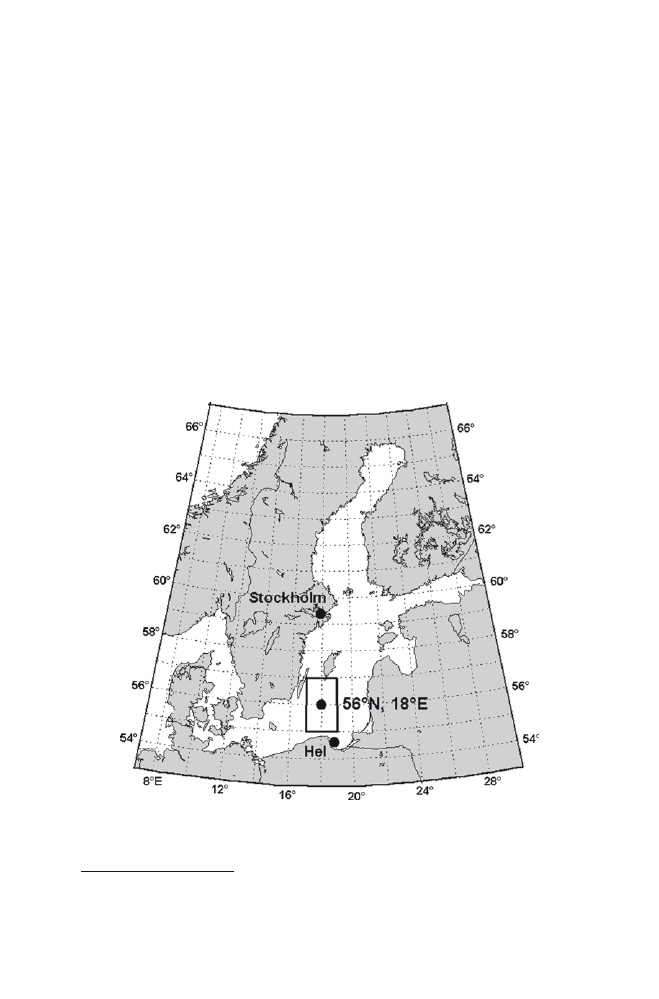
The analysis of changes in SST in the Baltic Sea made use of a grid with coordinates

56°N, 18°E whose time series describes the mean SST defined within the limits
55–57°N, 17–19°E. The surface area of the sea area calculated as a flat area is
27,618 km

2

. Figure

16.1

presents the location of this surface. The described sea area

almost in 100% covers water surface and characterizes open waters of the southern
part of the Baltic Sea.

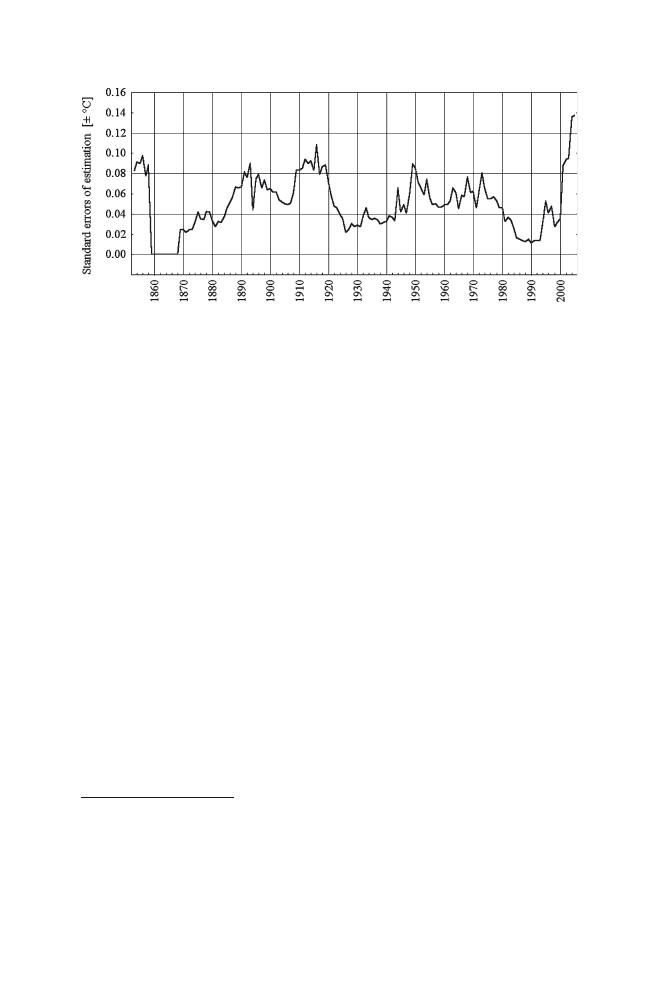
The standard estimation error for the mean monthly SST in the examined sea

area in most cases is within the range from ±0.01 to ±0.04°C, maximum errors
reach ±0.61°C (data set NOAA NCDC ERSST version2 err). Figure

16.2

presents

the distribution of estimation error for annual SST calculated as mean value of
monthly errors in a given year. The highest values of standard estimation errors for
monthly temperature, except for single cases, are noted in April.

The values of annual temperatures used for this analysis were calculated from

the values of mean monthly temperatures as mean arithmetic values. Changes in
annual SST in this grid point are very strongly correlated (r = 0.97–0.99)

6

with

Fig. 16.1

The location of areas whose mean annual temperatures were analysed in this work.

Grid 56°N, 18°E is marked with black point

6

r – Pearson’s linear correlation coefficient.

359

16 Changes in Sea Surface Temperature of the South Baltic Sea (1854–2005)

the changes in SST in the adjacent to the examined grid points and this makes it
possible to state that they are representative for a far greater sea area than the
examined surface.

The data showing the air temperature from Stockholm station up to 1889 are

derived from the data set GHCN v.2 (Peterson and Vose

1997)

and for the year

1890 from the data set Nordklim (Tuomenvirta et al.

2001)

The data character-

izing the temperature at Hel till the year 1995 are taken from the work by
Mi

ętus

(1998)

and in the following years they were supplemented with official

data from IMGW. The quality of these data has been checked by the authors of
these series and they are homogeneous. The values of NAO indexes used in this
work are taken from the data set accessible in official web sites WWW CRU
and J. Hurrell.

This work made use of standard methods in statistical analysis; when analyzing

signals a standard analytical methodology of electrical courses was employed
(Osiowski and Szabatin

1995)

. The principle of this method is that the following

elements are analyzed one by one, that is the course of deviation from the mean
value, low and up band signal envelopes whose aim is to define the components of
modulation, spectral analysis of a signal whose aim is to define spectrum of modu-
lating harmonic and harmonic being beating-up of modulating signals

7

and identi-

fication of impulse interference.

Fig. 16.2

Distribution in time of standard errors of estimation of mean annual SST in grid

56°N, 18°E

7

In case when two (or more) signals are received in the summing up system, processes of beat-

ing up (mixing) of signals forming new harmonics are observed. The basic harmonics of beating
up are the sum and difference between primary frequencies. In case when certain phase shifts
between primary signals are present, the amplitude of beating up harmonics can be higher than
the amplitude of modulating signals. The summing up system in this case is the surface layer of
the sea.

360

A.A. Marsz and A. Styszy

ńska

16.3 The Course of Mean Annual Value of SST

of the Baltic Sea

In the examined 152-year period the mean annual SST is 8.83°C (

sn = 0.61; sn – standard

deviation). The range of changes in SST is found within the limits from 10.17 (year
1990) to 6.76°C (year 1941) which result in an amplitude equal 3.41°. The course of
SST indicates to a great interannual changeability with clearly marked many-year
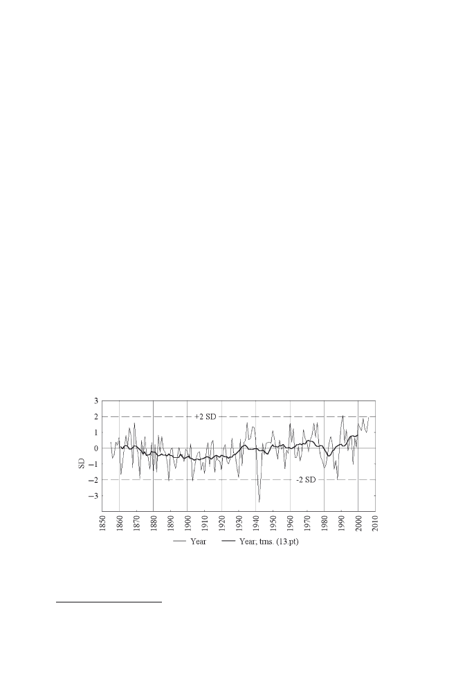
changeability. In order to define the periods of changes in SST it is more convenient
to use the standardised

8

course of SST (Fig.

16.3

). It can be easily noticed that the

characteristic feature of the course of SST in the examined period is asymmetry
noted in the frequency of the decreases in SST below −1 and −2

sn in relation to

how frequently the limits +1 and +2

sn are exceeded.

Over the period from 1854 to 1933 the frequency in SST drops below −1

sn and

is significant (20 times, twice, in this number, the limit was exceeded below −2

sn),

whereas the frequency of exceeding the limit +1

sn by SST is scarce (twice and in

this number 0 cases when the limit +2

sn was exceeded). From the year 1934 the

situation changes, that is more frequent are the cases when SST exceeds the limit
+1

sn (18 such cases including the one above +2 sn) when compared to situations

when the temperature drops below −1

sn (nine cases including the one below −3

sn). At the turn of 1933/1934 a clear change in the character of the changeability
(rhythm) of SST can be observed. In the first period a year-to-year changeability in
SST characterised by not too large amplitude can be noted with the 2–3 year peri-
odicity and majority of negative deviations. In the second period (1934–2005) the
5–10 year periodicity is noted and is characterised by large or very large amplitude
with majority of positive deviations, thus the year-to-year changeability in SST

Fig. 16.3

The course of standardized annual SST (in relation to 100-year period 1901–2000) in

grid 56°N, 18°E. Marked levels +2 and −2

sn (SD). Bold line – course adjusted by 13-point

moving average

8

Standardization was carried out with reference to mean 100-year value from 1901–2000.

361

16 Changes in Sea Surface Temperature of the South Baltic Sea (1854–2005)

recedes into the background. The negative deviations of SST become more significant
than in the former period and take evidently more time.

The course of cumulated deviations from the mean annual many-year value

makes it possible to distinguish the following periods in the course of annual
SST:

1. The years 1854–1875 – the mean annual value of SST is slightly higher that the

mean value of the entire period (~8.88°C), stable in time course of SST (trend
around 0; −9.974 ·10

−5

°C/year)

2. The years 1876–1932 – the mean annual value of SST is slightly lower than the mean

value of the entire period (~8.56°C), the cooling period (trend −0.002°C/year)

3. The years 1933–1939 – sharp increase in SST, the mean value significantly

higher than the mean value of the whole period

9

(9.45°C), trend +0.029°C/year

4. The years 1940–1947 – dramatic cooling, the mean SST value lower than the

mean of the entire period (8.41°C), trend −0.013°C/year

5. Years 1948–2005 – gradual increase in SST interrupted by periods of strong

cooling, the mean SST, the mean value higher than the mean value of the whole
period (~9.10°C), trend +0.009°C/year

If we take the strong cooling period in the 1940s as the minimal value of the course,
then the observed in 1941 the absolute minimum, will divide the examined period
into two parts, that is the one during which the decrease in SST (−0.002°C/year)
was noted and the mean SST is about 8.7°C and the other period in which the
increase in SST (+0.012°C/year) is observed and the mean SST is about 9.0°C.

Very strong fluctuations of SST which were observed between the beginning of

the 1930s and the end 1940s raise a question about the true limit between both great
periods of changes in temperature of the Baltic surface. The analysis of the course
of SST in which the short term fluctuations are neglected or/and their amplitude is
decreased (adjusted by 13 point moving average), will make it possible to set the
limit between these two periods at the turn of 20s and 30s of the twentieth century
(see Fig.

16.4a

). The warming period in the 1930s, despite being followed by a

period of strong cooling of the sea surface, ‘fits’ the pattern of following warming
which is characterised by the fact that the following increases in SST are higher
than decreases in SST, even if they are significant. Tentatively it can be assumed
that the limits between these periods can fall in the year 1929 which divides the
whole period into two equal parts. In such a case in the period 1854–1929 a
decrease in annual SST (−0.0065°C/year, p < 0.013), can be noted, whereas in the
period 1929–2005 an increase, a little higher than the previously observed decrease,
(+0.0072°C/year, p < 0.030) is noted.

The annual temperature resulting from averaging monthly values of SST

depends on changes in these values. In the course of SST observed in the sub-polar
latitudes, the annual temperatures are influenced by the heat resources left in the
waters after winter cooling of the sea surface as well as by the increase in heat

9

Rapid increase in SST in this period causes that the entire decade 1931–1940 is clearly warmer

than the average temperature; see Hansson and Omstedt

(2008)

.

362

A.A. Marsz and A. Styszy

ńska

resources in the sea surface at the end of the summer warming period. In the analysed
sea area the maximum SST can be observed in August and July or even in
September. The minimum value is noted in March, February or April and excep-
tionally, in some years in January.

The correlation between the annual SST with the mean values noted in winter

cooling periods (mean January–March) and the maximum summer warming (July–
September) is very strong in the examined area. It is described with the following
formula:

(

)

(

)

(

)

A

W

S

SST

1 103

0 339

0 395

0 029 • SST

0 406

0 023 • SST

.

.

.

.

.

.

,

=

±

+

±

+

±

(1)

where:

SST

A

– mean annual SST in the sea area within the limits of 55–57°N, 17–19°E; °C,

SST

W

– mean SST in the sea area as above from the period January–March

(winter),

SST

S

– mean SST in the sea area as above from the period July–September

(summer).

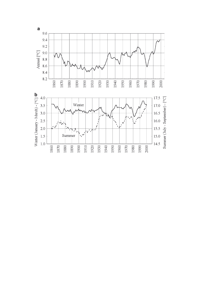
Fig. 16.4

The course of SST in grid 56°N, 18°E adjusted by 13-point moving average. (a) the

course of annual mean SST, (b) the courses of mean SST from the winter cooling (January–
March) and summer warming (July–September) of the sea surface. Note – please pay attention to
different scaling of SST in each part of the drawing

363

16 Changes in Sea Surface Temperature of the South Baltic Sea (1854–2005)

This correlation explains 84% of annual variances of SST (R = 0.91, F(2,149) =

385, p < 0.0000).

10

In this formula the summer SST variability explains 63% and

winter SST variability 21% of mean annual SST variances.

In order to illustrate to what extent the process of winter cooling and summer

warming periods affect the annual changeability in SST in the examined sea area,
the courses of changes in SST

W

and SST

S

adjusted by 13-point moving average are

presented (Fig.

16.4b

). This problem is not to be discussed here. At this stage what

is pointed out are the different courses of both components and the increasing
amplitude of winter and summer SST as a function of time. It should also be under-
lined that summer SST is correlated with winter SST. After the period of winter
cooling some smaller or bigger residual heat resources in water are left and they
have significant influence on temperature, the water reaches at the end of the sum-
mer warming of the sea surface. In the entire, 152-year, series changes in winter
mean value of SST (January–March) explain about 10% variances of mean summer
SST (July–September) (R ~ 0.3, F(1,151) = 16.4, p < 0.0001). This means that after
winter season, when there was lower heat absorption from the sea surface (which
is represented by higher SST in March–April), summer SST is higher; the course
of winter SST affects the course of summer SST. The changeability in mean winter
SST explains about 49% of mean annual SST variances (R = 0.7, F(1,150) = 141,
p < 0.000001). If we take into consideration additional influence of winter SST on
summer SST then, it turns out that changes in temperature during the winter cool-
ing of the sea surface have important influence on the annual SST. This winter SST
depends on weather phenomena present in a given winter.

16.4 Correlation Between Sea Surface Temperatures with NAO

Annual SST of the Baltic indicates strong correlation with the processes of heat
absorption in winter season. Because winter atmospheric circulation affects the
temperature of air transported over the sea, its humidity and the speed of the wind
it has influence on the amount of heat absorbed from the sea surface. That is why
the annual SST of the Baltic is relatively strongly correlated with different circula-
tion indexes which characterize the course of winter atmospheric circulation
(Koslowski and Glaser

1999

; Chen

2000

; Marsz and Styszy

ńska

2000, 2003

;

Omstedt and Chen

2001

; ACCBSB

2008

; Hansson and Omstedt

2008)

.

Because of the length of the analysed series, the only possible index of winter

atmospheric circulation to be used and to cover the whole period is NAO CRU
index (Gibraltar – SW Iceland; Jones et al.

1997)

, whose series starts in 1823.

Winter Hurrell index (Lisbon – SW Iceland; Hurrell

1995)

commences 10 years

later than the beginning of the analysed series of SST – namely in 1864.

10

R – multiple regression coefficient of correlation, F – value of Fisher-Snedecor test (in brackets

degree of freedom), p – statistical significance level (probability of random result).

364

A.A. Marsz and A. Styszy

ńska

In the whole series (1854–2005) averaged for the period January–March NAO

CRU index is correlated with annual SST of the Baltic Sea and this correlation is
highly significant (p < 0.00001), however the strength of this correlation is moder-
ate (r = 0.4156). Calculated for the same period as the Hurrell index was, that is
(December–March), the NAO CRU is correlated with the annual SST with a similar
strength within the whole examined period (r = 0.4049, p < 0.00001). Similar value
(r = 0.4277, p < 0.00001) is obtained for a series 1864–2005 (142 years) for a cor-
relation of annual SST with Hurrell NAO index which is calculated as a mean value
from the period December–March.

The analysis carried out for the following 30-year periods of correlations

between annual SST and winter NAO CRU index calculated for the period July–
March and NAO Hurrell index indicated that they are not stationary. The results of
the analysis are presented in Table

16.1

.

It has been noted that correlations with NAO CRU index were gradually

strengthened in the following 30-year periods, changing from relatively weak and
insignificant ones to very strong and statistically very significant. Similar correlations
between annual SST and NAO Hurrell index indicate similar course in the following
30-year periods but also here the strongest and most significant correlations are
observed in the 30-year period 1971–2000. These differences in the strength of the
correlation between SST and both NAO indexes result from different places of the data
(Gibraltar, Lisbon) used to create each of these indexes; generally speaking, for the
Baltic Sea it is the Hurrell index which provides more precise information about the
advection from the sector W-SW (Marsz and Styszy

ńska

2000)

.

Weak and statistically not significant correlations of annual SST with NAO

CRU index register the situation when the Iceland Low activity was relatively little
and the Azores High was located westward causing that the frequency of advection
of warm air masses from the Atlantic towards the Baltic Sea in winter was
restricted. The research carried out earlier (Marsz and Styszy

ńska

2000)

indicate

that in the period from the latter part of the 1860s till the last years of the nineteenth
century the Iceland Low was relatively weak. In that period a far greater role had
depressions over the Scandinavian Peninsula, which were closely connected with
strong advections of cold air from NW-NNW, than that of NAO in the process of

Table 16.1

Values of coefficients of correlation between annual SST and

winter NAO CRU index and NAO Hurrell index (r) and the level of their
statistical significance (p) for the following 30-year periods. Statistically
significant values of correlation are in bold

Period

NAO CRU Index

NAO Hurrell Index

N

r

p

r

p

1854–1880

0.3027

0.125

–

–

27

1881–1910

0.3173

0.088

0.4152

0.022

30

1911–1940

0.3315

0.074

0.3589

0.051

30

1941–1970

0.5618

0.001

0.3658

0.047

30

1971–2000

0.7233

0.00001

0.6844

0.00001

30

365

16 Changes in Sea Surface Temperature of the South Baltic Sea (1854–2005)

winter cooling of the Baltic. Only in the years 1902–1903 a rapid drop in atmospheric
pressure was observed in the region of Iceland during winter season.

11

The Icelandic

Low activated rapidly. However, the Azores High started moving east and north
east already from 1895. In winter more often than previously warm air was trans-
ported from the W sector to SW sector and not as it used to happen before from
NW-NNW; this was connected with positive phases of NAO. This case was noted
by statistically significant correlation of SST with Hurrell index in the period
1881–1910 but it was not noted by correlation with NAO CRU.

12

At the turn of the

20s and 30s of the twentieth century the activity of the Icelandic Low decreased
again; the course of winter cooling of the Baltic was influenced by different than
NAO circulation processes. At the same time the structure of synoptic processes
changed into favourable for warming the ocean surface in summer (strong conti-
nentalization). As a result correlations between annual SST and both NAO indexes,
although not changing the sign, they stop being statistically significant.

In the following two 30-year periods (1941–1970 and 1971–2000) the activity

of NAO increased gradually and this led to the increase in the strength and level of
correlation significance between annual SST and NAO. Especially during the last
30-year period (1971–2000) the processes of winter cooling of the surface of the
Baltic Sea were influenced by advection of sea air from SW and W controlled the
NAO. During this time NAO indexes indicated very high ‘concentration in time’ of
high positive values (years 1973, 1981, 1983, 1989–1990, 1992–1995, 1999–2000)
and also positive indexes, with values not observed during the whole preceding
process of instrumental observations, were noted (years 1989 (5.08); 1990 and
1995 (3.96-twice). In these years ‘winters without winters’ occurred over the south
and central Baltic during which the heat absorption from the sea surface was much
lower, leaving far greater resources of residual heat in waters. As a result a very
high increase in annual SST took place.

The last years (2000–2005) and especially last year (2006) for which there are

still some data lacking seem to be different from a pattern of changes in SST typical
of the last several dozen of years. The winter cooling intensity increased, when
compared to preceding years characterized by very high NAO indexes during win-
ter. However, they still remain weaker than during the last several dozen of years.
On the other hand, the intensity of summer warming processes increased consider-
ably when compared to last several dozen of years and this can result from the
increased frequency of occurrence of heights accompanied by advection of air
masses from SW. High temperature and relatively high humidity of air flowing over

11

In the years 1902 to 1903 there was a decrease in winter (July–March) pressure over SW Iceland

from ~1004 hPa to ~991 hPa. After the year 1903 the pressure over the SE Iceland started gradu-
ally increasing but the level from the years 1870–1900 then was observed as late as at the turn of
20-ties and 30-ties of the twentieth century.

12

In situation when the Azorean High moves NE, the pressure in Gibraltar can be relatively low

(Gibraltar S of the edge of the high) and the value of the NAO CRU index is lower, whereas
barometric gradient between Icelandic Low and Azorean High becomes strong (the decreased
distance between both atmospheric activity centres) and the sea air is transported farther E-NE
than in situation with the centre of the Azorean High locates over the Azores.

366

A.A. Marsz and A. Styszy

ńska

the Baltic are accompanied by clear decrease in wind speed and lower cloudiness
(effect of stable balance). All this leads to significant reduction in heat loss for
evaporation and turbulent exchange resulting in clear increase in SST at the end of
the summer warming period and this, in turn, results in high SST in autumn and at
the beginning of winter.

16.5 Correlations of SST with the Frequency of Occurrence

of Synoptic Situations of a Certain Type

It can be assumed that the annual temperature of the Baltic Sea surface should
indicate correlations with synoptic situations present over this sea area. From the
point of view of the mechanisms responsible for the changes in SST, it seems inter-
esting to define what synoptic situation was and when it had the greatest influence
on the value of SST. In order to provide answers to these questions an analysis of
correlations between the frequency of atmospheric circulation of Osuchowska-
Klein types (1978, 1991) and annual SST in the examined grid was carried out
(Osuchowska-Klein

1978, 1991)

. This analysis, because of the fact that the cata-

logue with low circulation types by Osuchowska-Klein comprises data from the
period from 1901 to 1990, does not cover the whole examined period of changes in
SST (1854–2005) but provides an extensive (90 years) although covering only 90
years, reliable sample of the occurring correlations.

This analysis was carried out in this way that it was assumed that the annual

SST (SST

A

) in a given examined period is the function of frequency of Osuchowska-

Klein, individual types of low circulation from January to December. The character
of this function is described by linear function (multiple regression). The consecu-
tive monthly frequencies (from January to December) of all circulation types
(A, CB, D, B, F, C2D, D2C, G, E2C, E0, E, E1 and BE) without type X (unmarked)
are taken as independent variables and that gives a potential equation with 156
independent variables. Using the method of gradual regression, taking F to use

³

10.0 and tolerance

³ 0.1, the values of constant term and regression coefficients

were estimated, limiting the number of independent variables of this equation to the
first four starting in the sequence of entering (more than 20 cases for one indepen-
dent variable). As a result of the above described procedure the following equation
is formed:

(

)

(

)

(

)

(

)

(

)

A

01

08

02

02

SST

8 4389

0 0094

0 0916

0 0179 E0

0 0633

0 0099

E

0 0876

0 0189 C2D

0 0795

0 0232 D2C

.

.

.

.

.

.

.

.

.

.

,

=

±

−

±

+

±

+

±

+

±

(2)

and its statistical characteristic is as follows: R = 0.72, adj. R

2

= 0.50, F(4.85) =

23.1, BSE = 0.44.

This relation indicates that 50% of variances of annual SST explain the fre-

quency of four types of lower circulation types- number of days with E0 circulation
type in January (E0

01

), E type in August (E

08

), C2D type in February (C2D

02

) and

367

16 Changes in Sea Surface Temperature of the South Baltic Sea (1854–2005)

D2C type in February (D2C

02

). The changeability in frequency: of E0 type in

January explains 16.3% of changeability in annual SST, E type in August – 17.1%,
C2D type in February – 12.1%, and of D2C type in February – 6.6%.

Equation [2] explains that the processes of winter cooling of the sea surface

(three out of four variables originate from the winter season) have the greatest influ-
ence on the changeability in annual SST. Such findings are compliant with the
earlier results of research into relations between the annual SST and winter and
summer SST and into the influence the winter atmospheric circulation has on the
value of annual SST. The determining influence of the frequency of circulation E
type in August (high pressure over the Scandinavian Peninsula and over the Baltic
during the maximum warming of the sea surface) and the frequency E0 type in
January (north-east and east anticyclone circulation during the most intensive win-
ter cooling) on the changeability of annual SST is both clear and comprehensible.
However, the great role of warm circulation types in February – C2D and D2C
which affect the changeability of annual SST is quite astonishing. The occurrence
of these circulation types in February restricts the heat absorption from water sur-
face thus, it makes further stronger decrease in SST impossible and in this way it
contributes to the increase in the residual heat resources in water after ‘winter’. The
increased number of these types of circulation in February eliminates also the
possibility of occurrence of other, ‘cooler’ types of circulations.

16.6 Relations of Air Temperature Over Coastal

Areas with SST

Changes in SST which cause that over vast areas exchange of heat between the
ground and atmosphere takes place, have direct influence on air temperature. What
is more, SST by having influence on the type of atmospheric balance and in this
way also on cloudiness may be said to have influence on the air temperature in an
indirect way. In turn, the air temperature by controlling the heat import from the sea
surface affects SST. In this way the courses of both physical values over a given
sea area are correlated with one another.

The air temperature over coastal stations quite accurately, though not perfectly,

reflects changes in SST. This work is limited to presenting the changes between
annual SST and annual temperature at two stations located close to the Baltic coast-
line, that is at Stockholm and at Hel. The courses of annual air temperature at the
stations located on the South and Central Baltic Sea are strongly correlated with
each other. Dealing with greater number of stations will not contribute to the
analysis.

In the whole, 152-year observational, period the coefficients of correlation

between annual SST and annual air temperature at Hel and Stockholm are almost
exactly the same (r equals 0.7611 and 0.7562 respectively) and what is obvious they
are highly significant. In the same period the annual temperature at Stockholm and
Hel indicates visibly stronger correlation (r = 0.8675, p < 0.000001). It should be

368

A.A. Marsz and A. Styszy

ńska

pointed out that the forced decrease in the amplitude of changes in SST in the range
of minus temperatures causes that the value of coefficient of correlation between
both annual values of temperature becomes lower and the correlation between
annual air temperature and SST cannot be perfect. It happens because SST cannot
drop below the freezing point/temperature of water of given salinity, whereas the
winter air temperature can fall considerably below 0°C.

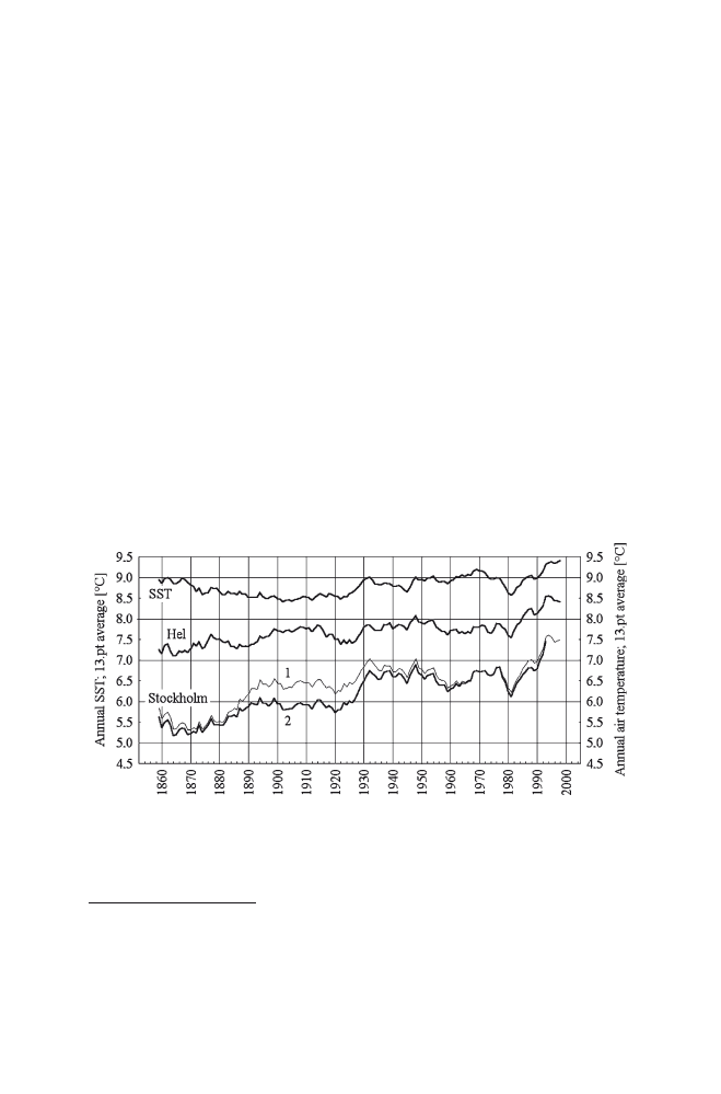
The course of annual air temperature at Stockholm and Hel stations and annual

SST adjusted by 13-point moving average is presented by Fig.

16.5

. It can be

clearly seen that there is considerable decrease in amplitude of SST in relation to
the amplitude of air temperature.

Greater discrepancies between the course of air temperature and SST are marked

at the initial segment of the examined course – more or less

13

to the 1920s. The air

temperature in this period increases and SST drops. Also in the period 1854–1894
more significant differences in the course of annual air temperatures between
Stockholm and Hel are noted. It is difficult to find the reasons for such discrepan-
cies at this stage. However, it is worth mentioning that the series of annual air
temperature at Stockholm before making the series homogeneous

14

shows clearly

fewer discrepancies with the course of annual SST in the period from 1900 to 1950,
and in the whole period 1854–2000 in which the data were not verified and made
homogeneous, the series is a little more correlated with annual SST (r = 0.7812,
p < 0.000001) than the verified series.

Fig. 16.5

The course of annual SST in grid 56°N, 18°E and annual air temperature at Hel station

and Stockholm (1 – homogeneous series, 2 – series not made homogeneous). The courses adjusted
by 13-point moving average

13

As both courses have been adjusted by 13-point moving average, more precise defining the limit

of discrepancies is unnecessary.

14

It a series from the period 1854–1995, from the year 1996 to 2000 amended with official data

from the station in Stockholm.

369

16 Changes in Sea Surface Temperature of the South Baltic Sea (1854–2005)

The analysis of correlations between annual air temperatures at Stockholm and

Hel and SST in the examined grid carried out for consecutive 30-year periods (the
same for which the analysis of correlations with NAO was made) indicates that
these correlations are non stationary in the function of time. The values of correla-
tion coefficients are presented in Table

16.2

.

It can be noted that the strength of the correlations of annual air temperature at

the Baltic stations is greatest in the 30-year period 1971–2000. As opposed to cor-
relation between SST and NAO in the years 1911–1940 when the strength consider-
ably decreased (see Table

16.1

), the relations between the air temperature and SST

in the same 30-year period were clearly stronger and the statistically significant
decrease in the strength of the correlations was observed in 30-year period 1941–
1970. Due to the fact that the period 1971–2000 is characterised by mild winters
and the period 1941–1970 by severe winters, it can be assumed that in the periods
in which there is an increase in the frequency of mild winters there is also stronger
convergence of the course of annual air temperature with the annual SST of the
Baltic Sea.

16.7 The Problem of Climatic Signal in Series of Values

of Mean Annual SST of the Baltic Sea

In order to explain what signal or climatic signals are carried in annual SST of the
Baltic Sea, the series was analyzed in a way that is typical of signals analysis used in
tracing courses of electric values (Osiowski and Szabatin

1995)

. Because it is not

clear what the interference and what the signal in the course of annual SST of the
Baltic Sea is, it is not acceptable to make any a priori assumptions in this respect.
That is why it is also unacceptable to employ preliminary filtering of the series of data
and the analysis is carried out on standard data without their further transformation.

The spectral analysis detects in the examined series presence of periodicity.

Apart from long term periodicity, equal to the whole length of the series (152
years), a half of the length (76 years) and a quarter of the length of the series (35.5

Table 16.2

Values of coefficients of correlation (r) between annual SST and annual

air temperature at Stockholm and Hel stations (Stockholm 1 – a series of data verified
and made homogeneous, Stockholm 2 – a series without statistical filtering) and Hel
(a series of data verified and made homogeneous) in consecutive 30-year periods. All
values of coefficients of correlation in the table are statistically significant with
p < 0.005, larger than 0.6 with p < 0.000
Period

n

Stockholm 1

Stockholm 2

Hel

1854–1880

27

0.6665

0.6612

0.5529

1881–1910

30

0.6085

0.7022

0.7287

1911–1940

30

0.8950

0.9044

0.8272

1941–1970

30

0.8098

0.8240

0.7381

1971–2000

30

0.9276

0.9262

0.9137

370

A.A. Marsz and A. Styszy

ńska

years), which are normal statistical artifacts connected with Fourier analysis, indicates
also short term periodicity. They ar e ~12.4-year periodicity, ~7.7-year periodicity,
~5.0- year periodicity and about 2-year periodicity.

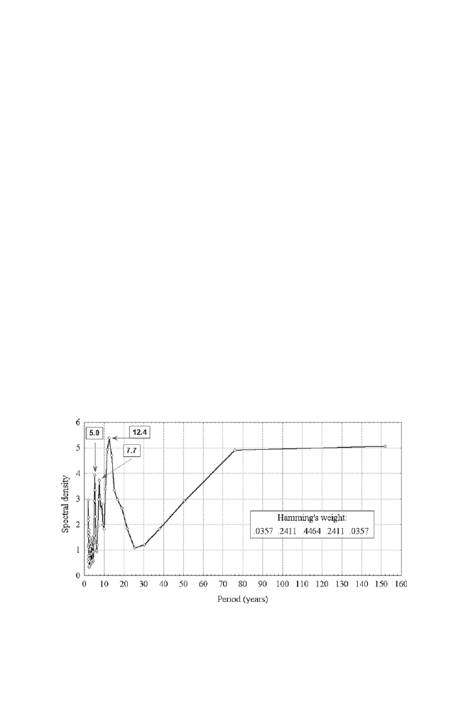
The 12.4 periodicity is dominating as far as amplitude is concerned; on a spectral

density scale it reaches the value of about 5.4 and is higher than all long term har-
monics (see Fig.

16.6

). Smaller amplitude can be noted in 7.7 – year and 5.0-year

periodicity (4.7 and 4.9 on the scale of spectral density respectively). The smallest
amplitude has the approximately 2-year periodicity (2.9 on the scale of spectral
density).

12.4-year periodicity whose peak is made up of 13.1-year, 12.4-year and 11.3-

year periodicities can be associated with the changing activity of the Sun. It falls
into the range 10–13 years characteristic for the variability of Wolf number whose
average periodicity in the years 1700–1995 was defined as 11.1 years. A great
number of works (e.g. Boryczka

1998

; Black et al.

1999

; White et al.

1997

;

Boryczka et al.

2001

; Coughlin and Tung

2004)

indicate that there are statistically

significant correlations between the changeability of the Sun activity and change-
ability of individual climatic elements and the intensity of some oceanic and tropo-
sphere processes. In spite of the fact that the changeability of solar constant
connected with the changeability of the Wolf number is very small (less or about
0.1% of the constant; Kristjansson et al.

2002)

and the changes in radiation can only

be observed in UV band, which causes that the mechanisms of this changeability
influence on the course of atmospheric processes are not clear, Foukal

(2002)

shows that these little changes in radiation explain about 20% variances of changes
in global temperature in the period 1915–1998.

The ~7.7-year periodicity, with the peak values of spectral density made up of

7.3-year, 7.7-year and 8.0-year periodicity can be associated with, so called,

Fig. 16.6

The results of spectral analysis of standardized annual SST (adjusted by 5-element

Hamming filter). The marked periodicity of peak values of spectral density (years)

371

16 Changes in Sea Surface Temperature of the South Baltic Sea (1854–2005)

‘quasi -8-year periodicity’,

15

commonly recognised from the course of air temperature

over Poland and the neighbouring regions (Ko

żuchowski and Marciniak

1994

;

Żmudzka

1995

; Boryczka

1998

; Ko

żuchowski

2000

; Fortuniak et al.

2001)

and

the course of some natural processes indicating stronger correlation with the
course of air temperature (e.g. sea ice formation; see Ko

żuchowski and

Girjatowicz

1997)

or with the increase in wind speed (e.g. the number of winter

storms over the Baltic Sea).

The quasi -8-year periodicity marked in the course of temperature is connected

with the course of circulation processes present over the region of the Atlantic and
NW Europe- primarily with NAO. Boryczka et al.

(2000, 2001)

define the periodic-

ity of NAO CRU index (Jones et al.

1997)

for the period from December to March

as 7.7-year periodicity and for one year as 7.8-year. Marsz

(1999)

finds 7.78-year

periodicity for one year in the course of Hurrell NAO index. Fortuniak

(2000)

appoints the limit of statistically significant quasi-7-year (7.37) periodicity in the
course of air temperature over Europe; the area of the South Baltic Sea is covered
by this scope.

The ~12-year and ~7–8-year periodicity are so strong that their presence can be

found in the course of annual SST of the Baltic Sea adjusted by 13-point moving
average. This kind of filtering, to a great extent, suppresses periodicity shorter than
13 years.

The ~5-year oscillation noted in the course of annual SST of the Baltic most

probably originates from beating up (sum) of basic harmonics; ~7.8 years and
~12.4 years. The occurrence of about 2-year oscillation in connected with the
changeability of SST of the Baltic Sea from year to year.

If the 12-year periodicity is really connected with the changing activity of the

Sun (Wolf numbers) then it would mean that this signal is most clearly marked in
periodical components of changes in annual SST. However, the changeability in the
number of sunspots in the examined period is very weakly correlated with the
course of the annual SST (r = 0.18, p < 0.02). The changeability of the number of
sunspots

16

explains only 3.3% variances of annual SST in the entire 152-year

period. The winter atmospheric circulation is on the second place with regard to
amplitude of modulating signal, despite being strongly correlated with the course
of annual SST, it explains a dozen or so % variances of SST in the same period.
It is a kind of paradox.

15

In a yearly course in a series made up of 152 consecutive values a strong signal of 7.7-year

period is detected. In the course of seasonal values of SST (January–March, July–September, and
October–December) and in monthly courses of the same duration statistically significant or less
frequently not significant periodicity falling into the periods from 8.09 years to 7.19 years can be
found. The authors think that too much attention should not be paid to slight differences in the
duration of the periods noted here. It is enough to change the length of the analyzed series
(shorten) by 1-5 and the spectral analysis detects in the same series periodicity about 0.1–0.3 years
different from the one defined earlier

16

Data from National Geophysical Data Center, Solar-Terrestrial Physics Division (E/GC2),

Boulder, Colorado.

372

A.A. Marsz and A. Styszy

ńska

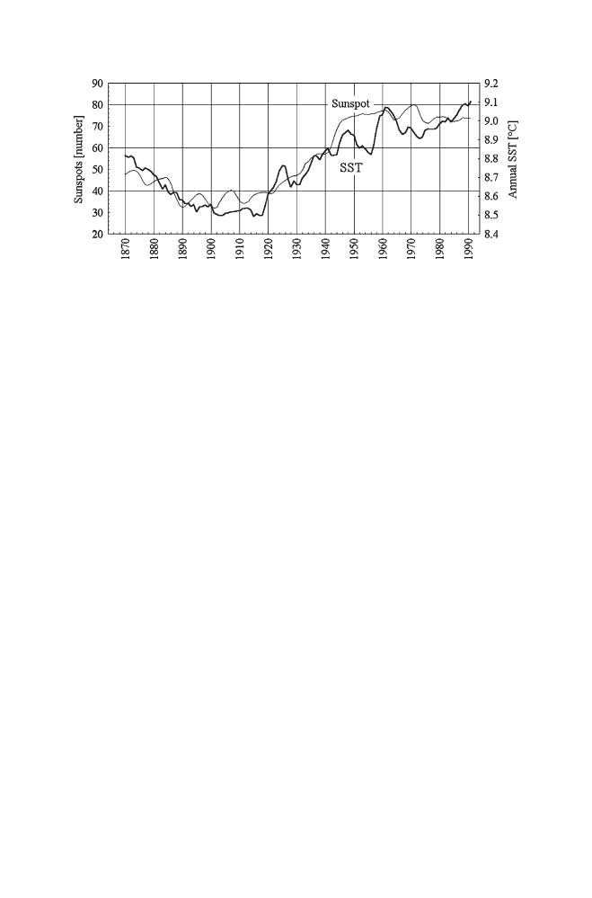
However, if the problem of long term activity of both modulating components is

considered, this paradox becomes even more puzzling. Because the periodicity con-
nected with the changing activity of the Sun falls within the limits of 11–13 years,
in order to filter this changeability and to find out sub-trends a longer filter of
doubled periodicity should be used. Here 31-point moving average of chronological
series of sunspots number and annual SST was used. The picture that is obtained
(see Fig.

16.7

) seems to suggest that the long term changeability in the number of

sunspots can really attribute, together with changeability in the character of winter
atmospheric circulation, to long term changes in SST of the Baltic Sea and influ-
ence the occurrence of long term sub-trends in series of SST. If this conclusion is
true, it can mean that the increase in annual SST from the 20s to the 30s of the
twentieth century can also be influenced by the increase in the Sun activity. The
same analysis carried out to explain if there are similar correlations between winter
(January–March) NAO CRU index and the changing activity of the Sun does not
find any correlations between these elements.

Acknowledgments

We would like to thank NOAA/OAR/ESRL PSD, Boulder, Colorado, USA,

for making from their website data set NOAA_ERSST_v2 available by ftp from WWW (

http://

www.cdc.noaa.gov/

). We would also like to express our gratitude to National Geophysical Data

Center, Solar-Terrestrial Physics Division (E/GC2), Boulder, Colorado, USA, for making series of
data with annual values of sunspots number in the period 1700–2005 available.

References

Assessment of Climate Change for the Baltic Sea Basin (2008) The BACC Author Team. Springer,

Berlin/Heidelberg

Betin VV, Preobraženskij YV (1962) Surovost’ zim v Evrope i ledovitost’ Baltiki. Gidrometeoizdat,

Leningrad (in Russian)

Black DE, Peterson LC, Overpeck JT, Kaplan A, Evans MN, Kashgarian M (1999) Eight centuries

of North Atlantic ocean atmosphere variability. Science 286:1709–1713

Fig. 16.7

Adjusted by 31-point moving average courses of annual values of SST in grid 56°N,

18°E and annual number of sunspots (1854–2005)

373

16 Changes in Sea Surface Temperature of the South Baltic Sea (1854–2005)

Boryczka J (1998) Zmiany klimatu Ziemi. Wydawnictwo Akademickie Dialog, Warszawa
Boryczka J, Stopa-Boryczka M, Lorenc H, Kici

ńska B, Błażek E, Skrzypczuk J (2000) Atlas

współzale

żności parametrów meteorologicznych i geograficznych w Polsce. t. XIV: Prognozy

zmian klimatu Warszawy, Wyd. Uniwersytetu Warszawskiego

Boryczka J, Stopa-Boryczka M, Baranowski D, Bła

żek E, Skrzypczuk J (2001) Atlas

współzale

żności parametrów meteorologicznych i geograficznych w Polsce. t. XV: Prognozy

zmian klimatu miast Europy. Wyd. Uniwersytetu Warszawskiego

Chen D (2000) A monthly circulation climatology for Sweden and its application to a winter

temperature case study. Int J Climatol 20(10):1067–1076

Coughlin K, Tung KK (2004) Eleven-year solar cycle signal throughout the lower atmosphere.

J Geophys Res 109. doi:

10.1029/2004JD004873, D21105

Fortuniak K (2000) Stochastyczne i deterministyczne aspekty zmienno

ści wybranych elementów

klimatu Polski. Wyd. Uniwersytetu Łódzkiego

Fortuniak K, Ko

żuchowski K, Żmudzka E (2001) Trendy i okresowość zmian temperatury powie-

trza w Polsce w drugiej połowie XX wieku. Przegl Geofiz 44(4):283–303

Foukal P (2002) A comparison of variable solar total and ultraviolet irradiance outputs in the 20th

century. Geophys Res Lett 29(23): 2089. doi:

10.1029/2002GL015474

Hansson D, Omstedt A (2008) Modelling the Baltic Sea ocean climate on centennial time scale;

temperature and sea ice. Clim Dynam 30:763–778. doi:

10.1007/s00382-007-0321-2

Hurrell JW (1995) Decadal trends in the North Atlantic oscillation: regional temperatures and

precipitation. Science 269:676–679

Jones PD, Jonsson T, Wheeler D (1997) Extension to the North Atlantic oscillation using early

instrumental pressure observations from Gibraltar and South-West Iceland. Int J Climatol
17(13):1433–1450

Koslowski G, Glaser R (1999) Variations in reconstructed ice winter severity in the Western Baltic

from 1501 to 1995, and their implications for the North Atlantic oscillation. Clim Change
41(2):175–191

Ko

żuchowski K (ed) (2000) Pory roku w Polsce: sezonowe zmiany w środowisku a wieloletnie

tendencje klimatyczne. Łód

ź

Ko

żuchowski K, Girjatowicz J (1997) Zmienność zlodzenia Zalewu Szczecińskiego na tle

współczesnych fluktuacji klimatycznych. Przegl Geofiz 42(2):155–167

Ko

żuchowski K, Marciniak K (1994) Temperatura powietrza w Warszawie: niektóre aspekty

zmienno

ści w okresie 1779–1988. In: Kożuchowski K (ed) Współczesne zmiany klimatyczne.

Klimat Polski i regionu Morza Bałtyckiego na tle zmian globalnych. Uniwersytet Szczeci

ński,

Rozprawy i Studia 152:19–46

Kristjansson JE, Staple A, Kristiansen J (2002) A new look at possible connections between solar

activity, clouds and climate. Geophys Res Lett 29(23):2107. doi:

10.1029/2002GL015646

Marsz A (1999) Oscylacja północnoatlantycka a re

żim termiczny zim na obszarze północno-

zachodniej Polski i polskim wybrze

żu Bałtyku. Przegl Geogr 71(3):225–245

Marsz A, Styszy

ńska A (2000) Fazy kontynentalizacji i oceanizacji klimatu nad obszarem Bałtyku

w XIX i XX wieku. Act Univ Nic Copernici, Geogr 31:183–201

Marsz A, Styszy

ńska A (2003) Zmiany temperatury powierzchni Bałtyku w rejonie Zatoki i Głębi

Gda

ńskiej (1871–1992) i ich związki z temperaturą powietrza. Prace Wydz Nawigacyjnego

Akademii Morskiej 14:100–137

Mi

ętus M (1998) O rekonstrukcji i homogenizacji wieloletnich serii średniej miesięcznej tempera-

tury ze stacji w Gda

ńsku-Wrzeszczu, 1851–1995. Wiad IMGW 21(2):41–63

Mi

ętus M, Filipiak J, Owczarek M (2004) Klimat wybrzeża południowego Bałtyku, stan obecny

i perspektywy zmian. In: Cyberski J (ed)

Środowisko polskiej strefy południowego Bałtyku.

Stan obecny i przewidywane zmiany w przededniu integracji europejskiej. GTN, Gda

ńsk

Omstedt A, Chen D (2001) Influence of atmospheric circulation on the maximum ice extent in the

Baltic Sea. J Geophys Res 106(C3):4493–4500

Osiowski J, Szabatin J (1995) Podstawy teorii obwodów. Wyd. Naukowo-Techniczne, Warszawa,

vol. 1, p 359, vol. 2, p 410

Osuchowska-Klein B (1978) Katalog typów cyrkulacji atmosferycznej. WKiŁ, Warszawa

374

A.A. Marsz and A. Styszy

ńska

Osuchowska-Klein B (1991) Katalog typów cyrkulacji atmosferycznej (1976–1990). IMGW,

Warszawa

Peterson TC, Vose RS (1997) An overview of the global historical climatology network tempera-

ture data base. Bull Am Met Soc 78:2837–2849

Siegel H, Gerth M, Tschersich G (2006) Sea surface temperature development of the Baltic Sea

in the period 1990–2004. Oceanologia 48(S):119–131

Smith TM, Reynolds RW (2004) Improved extended reconstruction of SST (1854–1997). J Clim

17(12):2466–2477

Soskin IM (1963) Mnogoletnie izmeneniya gidrologi

českikh kharakteristik Baltijskogo morya.

Gidrometeoizdat, Leningrad

Terziev FS, Rozhkov VA, Smirnova AI (eds) (1992) Proekt “Morya SSSR”. Gidrometeorologiya

i gidrokhimiya morej SSSR. T. III. Baltijskoe Morye vyp. 1 Gidrometeorologi

českie usloviya.

Gidrometeoizdat, St. Petersburg

Tuomenvirta H, Drebs A, Førland E, Tveito OE, Alexandersson H, Laursen EV, Jónsson T (2001)

Nordklim data set 1.0 – description and illustrations. DNMI Report KLIMA 08/01

White WB, Lean J, Cayan DR, Dettinger MD (1997) Response of global upper ocean temperature

to changing solar irradiance. J Geophys Res 102(C2):3255–3266

Zblewski S (2006) Zmiany temperatury powierzchni Bałtyku w okresie maksimum globalnego

ocieplenia (1982–2001). Dissertation, Gdynia/Toru

ń

Żmudzka E (1995) Tendencje i cykle zmian temperatury powietrza w Polsce. Przegl Geofiz

40(2):129–139