C. Zeitnitz 09/2009

Manual for the sound card oscilloscope V1.32

C. Zeitnitz

english translation by P. van Gemmeren, K. Grady and C. Zeitnitz

This Software and all previous versions are NO Freeware!

The use of the software and of the documentation is granted free of charge for private and non-

commercial use in educational institutions.

Any commercial application, distribution and sale is prohibited.

For commercial usage contact the author!

All rights reserved.

© C. Zeitnitz 2005-2009

Web-page:

http://www.zeitnitz.de/Christian/scope_en

The sound card oscilloscope is a digital oscilloscope with an integrated signal

generator, frequency analysis (FFT) and wave file recorder

1 Requirements

• Windows 2000 , XP, Vista or Windows 7

• A PC with a sound card installed.

• 50MB of disk space

2 Installation

Unpack the ZIP file in any directory and run setup.exe. The program can be started thereafter through the
program menu of the Windows operating system.

3 Description

This software can be used for the display and analysis of sound waves. The data can be recorded both
directly from the sound card (with a microphone or LINE input), or from a source such as a CD or
Mediaplayer. The input to the oscilloscope is defined by the Windows sound mixer (see below). The software
obtains its input data for the sound card via the Windows interface. It does not communicate directly with the
sound card. Therefore sound card problems should be troubleshot at the operating system level.

The user interface is arranged like a conventional oscilloscope. However, in the program window, additional
XY display, frequency analysis, and settings are provided.

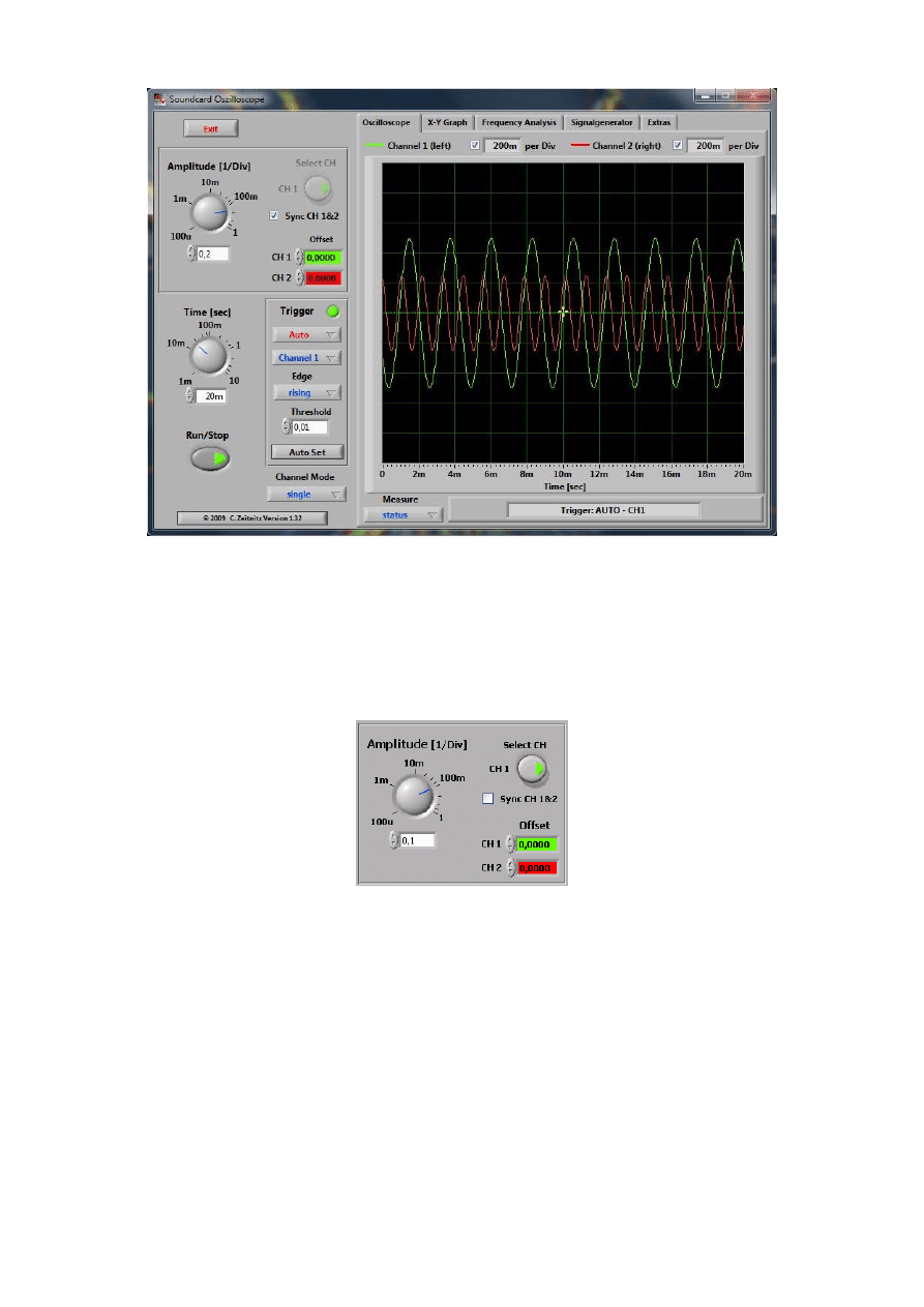
3.1 Oscilloscope

The software shows the left and right channel of the sound card in the oscilloscope window. The left channel
is represented as a green line and the right channel as a red line. In the user interface window there are
knobs and input windows for the following three functions: Amplitude, Time, and Trigger.

1

C. Zeitnitz 09/2009

Figure 1: Soundcard oscilloscope

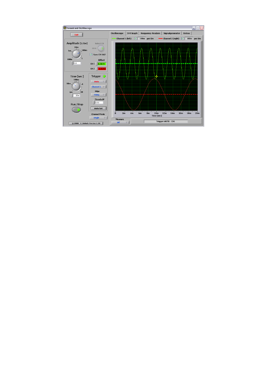
3.1.1 Amplitude

settings

The amplitude scale of the two channels can be set independently as well as synchronized. The latter is
enabled at program start-up and can be disabled by un-checking “Sync CH 1&2” on the front panel. In the
case of independent channel control, the active channel has to be selected by the button “Select CH” (see
Figure 2).

Figure 2: Amplitude settings and channel offsets

The amplitude values are given in units per division of the oscilloscope screen and are displayed for both
channels above this screen. The amplitude value corresponds to the digitized sound level divided by 32768.
This represents the 16Bit resolution of the data, which are taken with the sound card. Due to the different
settings of the volume in Windows the absolute sound level cannot be determined directly! Therefore the
presented values are to be understood in arbitrary units. The amplitude setting refers both to the
oscilloscope window and to the XY graph. An offset can be assigned to each channel individually via the
appropriate input window; thereby the two traces can be separated from each other. A click into one of the
offset fields will result in two horizontal cursors to show up in the oscilloscopes screen. The offset can now
be changed by moving these cursors with the mouse, or by entering a value into one of the fields. If the
signal of the channel is outside the visible window of the screen, the cursor is shown at the upper or lower
edge of the screen (dependent where the actual signal is located). The cursors will automatically disappear
from the screen after a few seconds without a change of an offset.

2

C. Zeitnitz 09/2009

Figure 3: Offset cursors visible on screen

3.1.2 Timebase

The Time setting refers to the entire represented range and NOT to the value per unit as with a normal
oscilloscope! The range goes from 1ms to 10,000ms. The larger the range, the smaller is the used scanning
rate. This is unavoidable because of the extent of computer cpu use. In the trigger setting "single" the
scanning rate is increased again, since computer utilization is less important here.

3.1.3 Trigger

The trigger setting modes are "off", "auto", "normal" and "single". These correspond to the standard modes
of oscilloscopes. The trigger threshold can be adjusted either in the input window of the trigger selection, or
by shifting the yellow cross in the oscilloscope window using the mouse. The trigger time can only be
adjusted by shifting the cross with the mouse.
In the single SHOT mode of the trigger the RUN/stop switch is deactivated automatically and must be
pressed again for a new data-taking run.
The button “Auto set” triggers the program to estimate the optimal time base and trigger level. The main
frequency found in the trigger channel is used to obtain the time base. The threshold is taken from the signal
amplitude. If the amplitude is too small, the button has no effect. Below approx. 20Hz the result is not reliable
due to the limited time window used for the analysis.

3.1.4 Channel

Mode

By default, two channels are shown in the oscilloscope window. With the mode selection switch at the
bottom of the program window, the sum, difference or product of the channels can be chosen.

3.1.5 Data

Analysis

On the user interface there is also a run/stop switch, which can be used to interrupt data taking to allow time
for analyzing the current window content. The selector “real time” allows to switch on a real time
measurements of the main frequency, the peak-to-peak amplitude and the RMS of the signal. The result is
displayed at the upper edge of the screen. This measurement requires some CPU power and should be
switched off, if any problems are observed.

3

C. Zeitnitz 09/2009

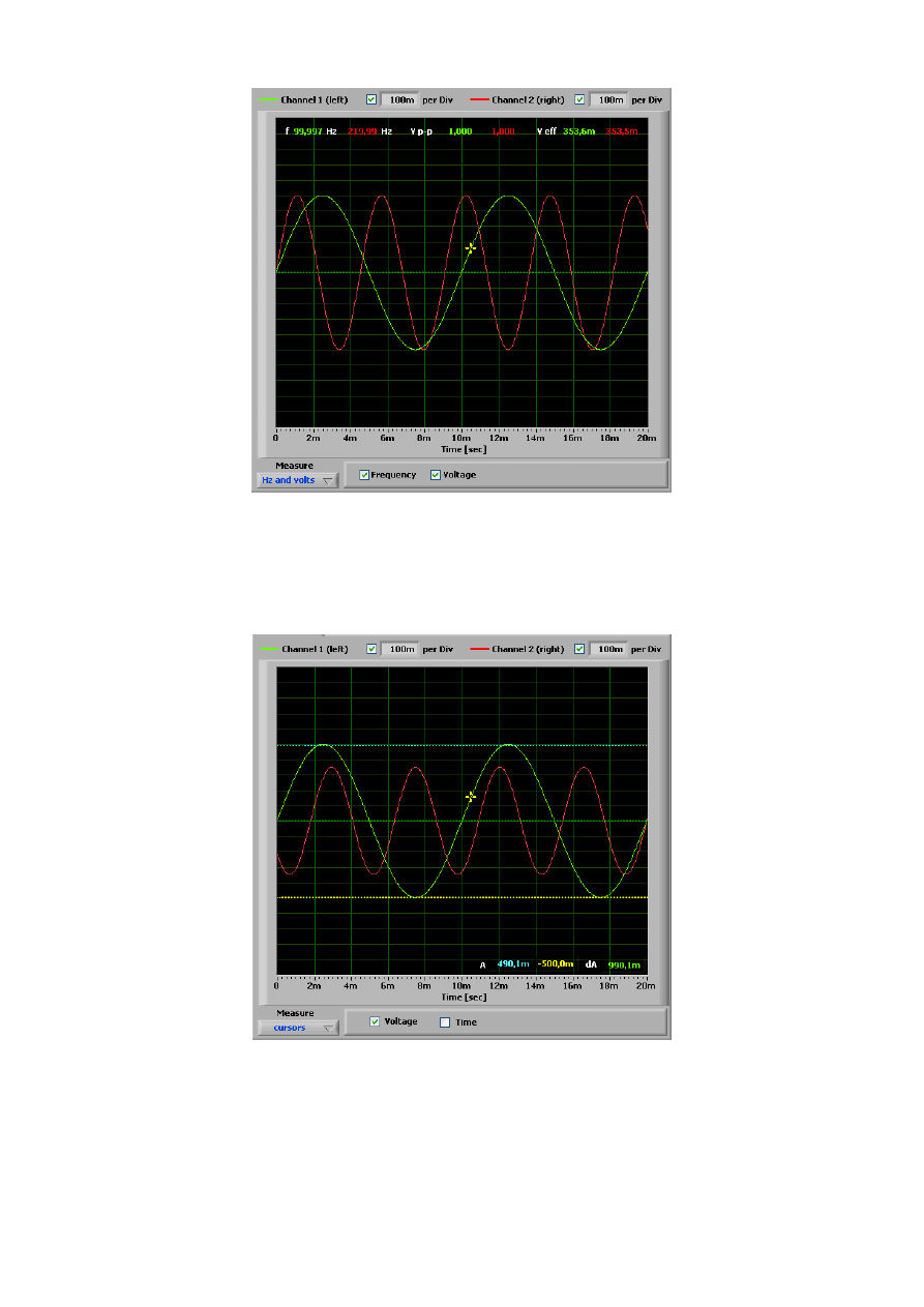
Figure 4: Automatic measurement of frequency and amplitude of signals

The amplitude or Time/frequency can be measured with the help of cursors in the oscilloscope window. The
corresponding cursors can be activated through the selector box underneath the window. The cursors can
be shifted with the mouse.
In the amplitude mode the values for the two cursors as well as the amplitude difference is displayed.

Figure 5: Amplitude analysis with the cursors. The shown values correspond to channel 1.

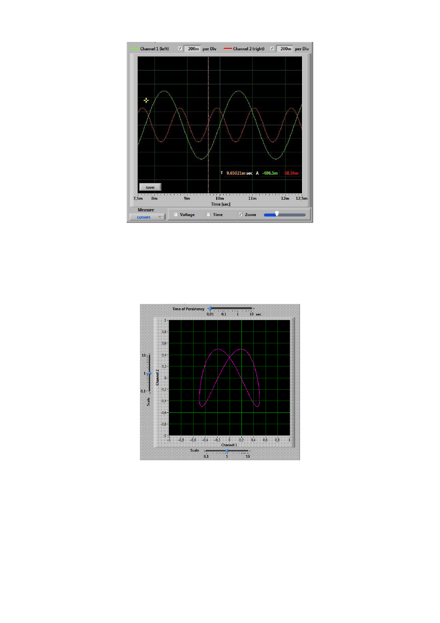
For the time mode the time difference and the appropriate frequency are shown directly. The data can also
be examined in more detail by using the zoom (only when the data acquisition is stopped). The detail around
the position of the orange cursor line is increased. By shifting the cursor the range can be changed.
Amplitude and voltage cursors can be enabled simultaneously.

4

C. Zeitnitz 09/2009

Figure 6: Zoom of the wave around the orange cursor with time and amplitude values displayed

The time position of the orange cursor and the corresponding amplitude values (green and red) are
displayed in the screen as well.

3.2 X-Y

Graph

Here the two channels are displayed against each other. Thereby e.g. Lissajous figures can be produced.
For this the frequencies can be adjusted in the signal generator.

Figure 7: Lissajous Figure for f1 = 440Hz, f2 = 880Hz and a phase of 45°

The slider above the graph allows to change the time of persistency of the shown data. For a longer time
setting increases the time window displayed on the screen. Fast changing signals should better be displayed
with a short persistency.
The controllers along the x and y axis permit a scaling of the appropriate channel (zoom in or out). The
represented range is chosen by adjusting the amplitude knob in the program window.

3.3 Frequency

Analysis

In the "frequency analysis" window, the display shows the result of the Fourier analysis of the selected
channel. The channel can be chosen with the selection button above the grid. By default, the graph shows
the amplitude of 0 - 10,000 Hz. The amplitude as well as the frequency can be displayed with a logarithmic
scale.

5

C. Zeitnitz 09/2009

The vertical scale can automatically be adjusted by selecting the auto-scale check-box above the graph. A
manual adjustment is possible by double-clicking the maximal or minimal value of the axis and entering a
new value. This should be done only if auto-scale is disabled.
Below the graph is a roll bar and a zoom sliding control; they permit the indicated range to be changed.
These should be only used if data taking has been stopped with the run/stop button. The zoom shot slider
shows details of the frequency analysis: use the mouse to set the perpendicular yellow line to the frequency
of interest and drive the zoom shot slider up to the desired detail.

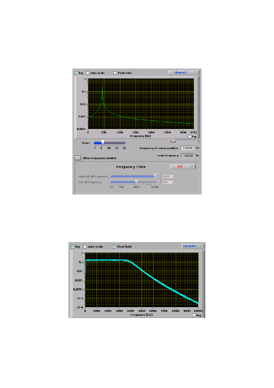
Figure 8: Frequency analysis of a 440Hz signal

The two output values underneath the sliders show the frequency at the cursor position and the value of the
strongest frequency found from a harmonious analysis of the data. Note that the Fourier analysis is always
based on data with the full sampling rate of 44.1kHz. Therefore, the time controller automatically jumps to a
pre-defined value when this window is active.
Selecting “peak hold” allows to store the maximal amplitude values of the Fourier analysis. This allows to
display the transfer function, when using the white noise generator.

Figure 9: Transfer function utilizing the peak hold function with the white noise generator

Under the frequency analysis an adjustable frequency-selective filter (Besselfilter 10th order) is also
provided. Three kinds of filter can be selected: Low-pass, high-pass and band-pass filter. The critical
frequencies can be adjusted with the sliding controls accordingly.
Above the frequency-selective filter is a button to open filter control in a separate window. This function
allows one to observe the effect of the filter directly in the oscilloscope window. Double-clicking on the button
or closing the window re-establishes the original settings.

6

C. Zeitnitz 09/2009

3.4 Transfer

Function

In addition to the frequency analysis of an individual channel it is possible to measure the transfer function.
This measurement uses the ratio of Channel 1 and Channel 2 to determine the frequency dependency of the
transfer characteristic. In order to obtain the transfer function one should select a noise signal or are square
wave in the signal generator in order to cover the full frequency spectrum in a single measurement.
Alternatively a frequency sweep can be utilized. Channel 1 should contain the original signal and the
Channel 2 the filtered one.

3.5 Storing Display Data

The graphics visible on the display (oscilloscope screen, frequency analysis, xy-graph) can be stored, when
the data acquisition has been stopped by the “RUN/STOP” button. A “save” button is displayed within the
graphs area. After pressing the button a file selector box is displayed to select a file name and the preferred
graphics format (BMP, JPG or PNG). Automatically the graph is saved in color and in black-white. In addition
a text file (extension CSV) containing the actual data is stored with the same name. This contains the data
as a Comma-separated-value list, which can be imported into Excel. Be aware, that the output to the CSV
file is localized and the decimal separator (comma or dot) is selected depending on your local settings.
Importing these data into Excel might lead to wrong results, if a different decimal separator is used.

3.6 Signal

Generator

A 2-channel signal generator is integrated into the program. The generator can be released from the
program window by pushing the button above the panel. A second click on the button will embed the
generator again.

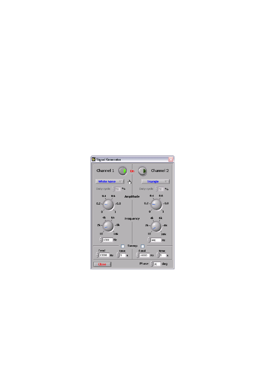
Figure 10: Signal Generator

The generator outputs sine, rectangle, triangle, and saw tooth waves with variable amplitude and frequency.
A white noise generator is included as well. The phase of the signal can be adjusted.
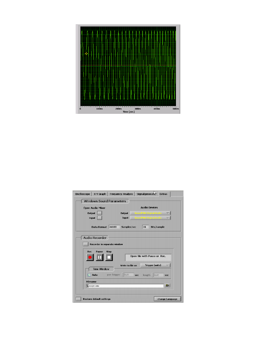
The “Sweep mode” allows to sweep the frequency from the main frequency to f(end) continuously within the
specified time window.

7

C. Zeitnitz 09/2009

Figure 11: Automatic frequency sweep

Upon opening the signal generator, both channels are deactivated and must be switched on by a button at
the bottom of the window. The frequency can be changed in steps of 0.5Hz. The generator signal can be
sent directly to the sound card. This must be activated in the sound mixer of the Windows operating system
(usually designated as "Wave Out"). If in addition the recording of the "Wave" source is activated, the signals
are visible in the oscilloscope and can be displayed (e.g. to produce Lissajous figures).

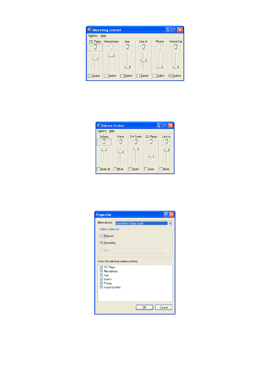
3.7 Extras

In this window, there are some settings for the Windows audio devices. On the right side are the audio
devices for sound input and output. If several sound systems are present, the equipment used can be
selected here.

Figure 12: Extras Tab contains the windows sound settings and the sound recorder

On the left side are buttons to start the Windows audio mixers operating. Note that each push of a button
opens a small mixer window! In the mixers, the inputs and outputs can be configured. At the bottom of the
settings window is a button to reset the program settings. This includes ALL settings; any changes made by
the user thus far will be lost!

8

C. Zeitnitz 09/2009

The language of the program can be with the corresponding button. The change of the language will be
applied at the next startup of the program

Figure 13: Language selection window

For experts only: The standard settings for the soundcard are 44.1kHz with 16Bit resolution per sample.
Higher sampling rates and sample resolutions can be set in the initialization file scope.ini located in the
installation path of the program. The corresponding parameters are “SamplingRate” and “Bits”, which are
commented in the original file. Most current soundcards (even onboard versions) support up to 100kHz and
16Bit. If the soundcard does not support the sampling rate and/or bit resolution, an error message will be
shown at program startup.
An additional parameter in the file scope.ini is the “MaxFrequency”, which determines the maximal value for
the displayed frequency in the Fourier analysis. The default value is 20000Hz. The sample length which is
analyzed by the Fourier analysis is by default 120 msec long. This allows to observe frequencies down to
approximately 20Hz. If you want to measure lower frequencies you can add the option
“FourierTimeWindow=500” into the scope.ini file. The number gives the sample length in milliseconds. Be
aware, that a large number slows down the update of the Fourier analysis substantially and requires more
CPU cycles.
Some sound cards invert the input signals before the digitization. This can be corrected by adding the option
“InvertSignal=true” in the scope.ini file.
In order to have a reasonable screen resolution when zooming in by a large factor, the resolution can be
increased by setting MaxSamplesScale to a value up to 100. This will increase the load on the system-

Addition information: be aware, that high sampling rate/bit rates and a high screen resolution can lead to a
significant CPU load. For 100kSample with 16Bit resolution the load is more than four times larger than
under standard conditions. So monitor the CPU load, when increasing the settings !

Here an example for an ini file:

SamplingRate=100000
Bits=16
MaxFrequency=20000
InvertSignal=TRUE
FourierTimeWindow=200
MaxSamplesScale=50.0

3.7.1

Signal Sources for the Oscilloscope

The following inputs are usually available:

• Line-In

Port on the PC

• Microphone Port on the PC, or internal (e.g. Laptop) – often only mono

• Wave Out

internal sound, e.g. MP3 player, Media-Player; signal generator

• CD Player

Music directly from a CD

The equipment to appear on the oscilloscope must be selected from the inputs mentioned above. With some
sound cards, several sources can be selected at the same time. The volume of the equipment can also be
adjusted here. This has a direct effect on the amplitude of the oscilloscope!

9

C. Zeitnitz 09/2009

Figure 14: Selection of inputs in Windows Audio Mixer

3.7.2

Signal Output via Sound Card

In order to define which sound is sent to the sound card output, the appropriate equipment must be selected
in the Windows Audio Mixer. Frequently several sources are merged at the same time here.

Figure 15: Selectable outputs

Important:
It can sometimes occur that an input or an output is not listed in the window. In this case it must be activated
under:

Æ Options ÆProperties

Figure 16: Properties of audio input devices

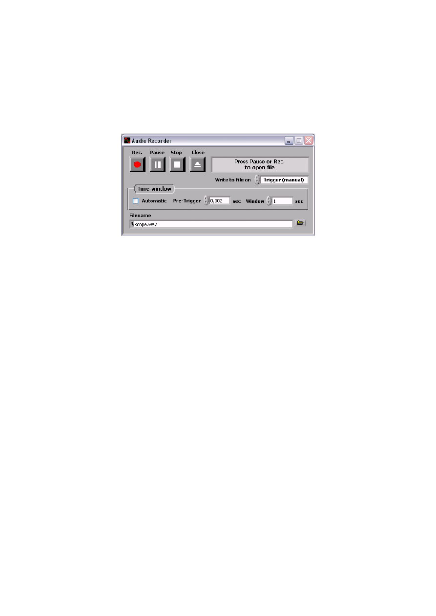
3.7.3 Audio

Recorder

The Audio Recorder allows to save data to a Wave file. The name of the output file has to be selected before
the Pause or Record button is pressed.
Three different modes are available to store data:

1. Trigger (auto)

Save automatically the currently triggered data

10

C. Zeitnitz 09/2009

2. Trigger (manual)

Manually save the last triggered data to the file

3. Rec. Button

Start the writing to the file with the record button (independent of the trigger)

Independent of the mode only a limited chunk size is written to the output file. The length is defined by the
corresponding selectors in the Recorders window. The length is by default defined by the oscilloscopes
window, but can be set by the user to a different value (uncheck the Automatic box). In all cases the writing
will stop, when Pause or Stop is pressed.
Be aware, that the selected file will be overwritten WITHOUT any warning! Since the current file will be
closed after the Stop button has been pressed, define a new output file BEFORE pressing Pause or Record!
The resulting Wave file will contain 100 samples of silence between the recorded data chunks. Cue points at
the beginning of the Wave file mark the start of each written chunk.

Figure 17: Audio Recorder window

4 Conclusion

I hope you will have a lot of fun with this program. If something goes wrong and you discovered a bug,
please send mail to [e-mail].
If you use the program for a project at and university or school I would like to know about it.

This program can be used and passed on for use within the school and private sector freely.
For planned commercial use please contact [e-mail].

5 Trouble

Shooting

Certainly this program might still have some errors, however some standard problems are caused by the
sound card and/or Windows.

An error message is shown when starting the program

The error message, that the installed LabView Run-Time engine (version 7.1) is incompatible with the
required one (version 7.1.1), is caused by a previously installed LabView Run-Time engine. In order to get
the program running, uninstall the Run-Time engine (Control panel

Î Add/Remove Program Î National

Instruments ) prior to a re-installing this software.

No soundcard is found

Check in the hardware manager, that Windows actually has a soundcard correctly installed. Some
soundcards recognize if speakers or a microphone is installed. This is the default behaviour under Windows
Vista/Win7. In this case you have to check, that at least one input/output device is enabled in the sound
settings (green check mark). If no output device is enabled, the program will complain about it and terminate
immediately.

The oscilloscope shows no signal and the display is frozen

Unfortunately it sometimes happens that communication with Windows breaks down. Here only terminating
and re-starting the program helps!

11

C. Zeitnitz 09/2009

No signal on the oscilloscope

If the signal generator is used and a channel is also SWITCHED ON, the user must select "Wave Out" for
the audio mixer equipment .

No sound audible

In order that a signal on the speaker is audible, the appropriate equipment must not be deactivated. In this
case check the audio mixer and enable the appropriate device. When using the signal generator, "Wave"
must be selected.

Strange jumps in the signal

A large signal can overdrive the input. The maximum possible value should actually be sent to the output.
With some sound cards, however, this leads to an overflow and instead of a large positive value, a large
negative value is sent, which leads to a complete distortion of the signal. If such jumps are observed, the
input signal should be attenuated

Program reacts very slowly

The CPU load on a slow computer (less than 1GHz) can go up to 100%, especially in the frequency analysis
mode. The program will only react slowly. A solution is to reduce the amount data to be processed by
changing the sampling rate in the file scope.ini. For this uncomment the line with the key word SamplingRate
and put in a value of 22050. This corresponds to a reduction of the amount of data by a factor of 4.
In the XY-view the persistence setting has a strong impact on the system load. You might have to reduce the
persistence time to obtain again a more responsive system.

12