C

H

A

P

T

E

R

17

F

IBER

O

PTIC

T

ESTING

J I M H AY E S

OVERVIEW

Testing fiber optic components and systems requires making several basic mea-
surements. The most common measurement parameters are shown in Table 17-1.
Optical power—required for measuring source power, receiver power, and loss
or attenuation—is the most important parameter and is required for almost every
fiber optic test. Backscatter and wavelength measurements are the next most
important, and bandwidth or dispersion are of lesser importance. Measurement
or inspection of geometrical parameters of fiber are essential for fiber manufac-
turers. And troubleshooting installed cables and networks is required.

Standard Test Procedures

Most test procedures for fiber optic component specifications have been stan-
dardized by national and international standards bodies, including the EIA in the
United States and International Electrotechnical Commission (IEC) or Interna-
tional Organization for Standardization (ISO) internationally. Procedures for
measuring absolute optical power, cable and connector loss, and the effects of
many environmental factors (such as temperature, pressure, flexing, etc.) are cov-
ered in these procedures.

179

In order to perform these tests, the basic fiber optic instruments are the fiber

optic power meter, test source, OTDR, optical spectrum analyzer, and an inspec-
tion microscope. These and some other specialized instruments are described
below.

Fiber Optic Instrumentation

Fiber Optic Power Meters

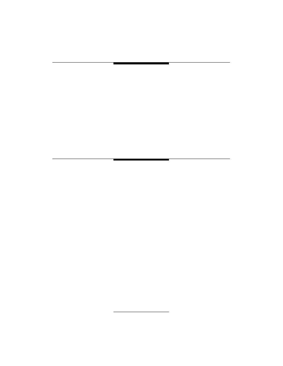
Fiber optic power meters (Figure 17-1) measure the average optical power ema-
nating from an optical fiber and are used for measuring power levels and, when
used with a compatible source, for loss testing. They typically consist of a solid
state detector (silicon [Si] for short wavelength systems, germanium [Ge] or
indium-gallium arsenide [InGaAs] for long wavelength systems), signal condi-
tioning circuitry and a digital display of power. To interface to the large variety
of fiber optic connectors in use, some form of removable connector adapter is
usually provided.

Power meters are calibrated to read in linear units (milliwatts, microwatts,

and nanowatts) and/or dB referenced to one milliwatt or one microwatt optical
power. Some meters offer a relative dB scale also, useful for laboratory loss mea-
surements. (Field measurements more often use adjustable sources set to a stan-
dard value to reduce confusion. See section entitled Fiber Optic Test Sources).

Power meters cover a very broad dynamic range, over 1 million to 1.

Although most fiber optic power and loss measurements are made in the range of
0 dBm to –50 dBm, some power meters offer much wider dynamic ranges. For
testing analog CATV systems or fiber amplifiers, special meters are needed with
extended high power ranges up to +20 dBm (100 mW).

180

CHAPTER 17 — FIBER OPTIC TESTING

Table 17-1

Fiber Optic Testing Requirements

Test Parameter

Instrument

Optical power (source output, receiver

Fiber optic power meter

signal level)

Attenuation or loss of fibers, cables, and

Fiber optic power meter and source, test kit or

connectors

optical loss test set (OLTS)

Source wavelength*

Fiber optic spectrum analyzer

Backscatter (loss, length, fault location)

OTDR

Fault location

OTDR, visual cable fault locator

Bandwidth/dispersion* (modal and chromatic)

Bandwidth tester or simulation software

* Rarely tested in the field

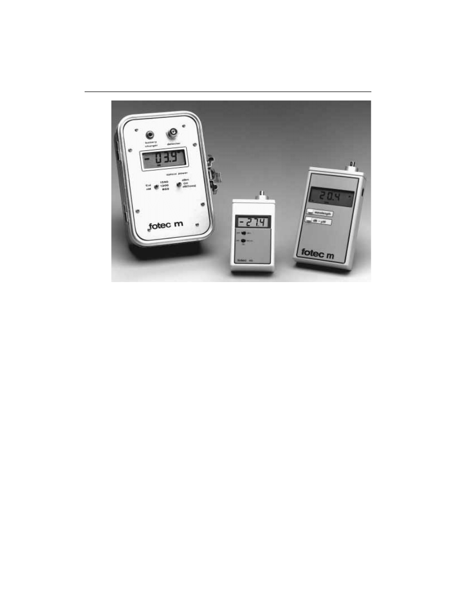
Figure 17-1

Fiber optic power meters come in rugged, mini, and handheld

packages. Courtesy Fotec, Inc.

Fiber optic power meters have a typical measurement uncertainty of ±5%,

when calibrated to transfer standards provided by national standards laborato-
ries such as the U.S. National Institute of Standards and Technology (NIST).
Sources of errors are the variability of coupling efficiency of the detector and con-
nector adapter, reflections off the shiny polished surfaces of connectors,
unknown source wavelengths (since the detectors are wavelength sensitive), non-
linearities in the electronic signal conditioning circuitry of the fiber optic power
meter, and detector noise at very low signal levels. Power meters with very small
detectors may have two problems that cause measurement errors. The light from
the fiber may overfill the detector or the detector may saturate at high power lev-
els. Since most of these factors affect all power meters, regardless of their sophis-
tication, expensive laboratory meters are hardly more accurate than the most
inexpensive handheld portable units.

Fiber Optic Test Sources

In order to make measurements of optical loss or attenuation in fibers, cables,
and connectors, one must have a standard signal source as well as a fiber optic
power meter. The source (Figure 17-2) must be chosen for compatibility with the

CHAPTER 17 — FIBER OPTIC TESTING

181

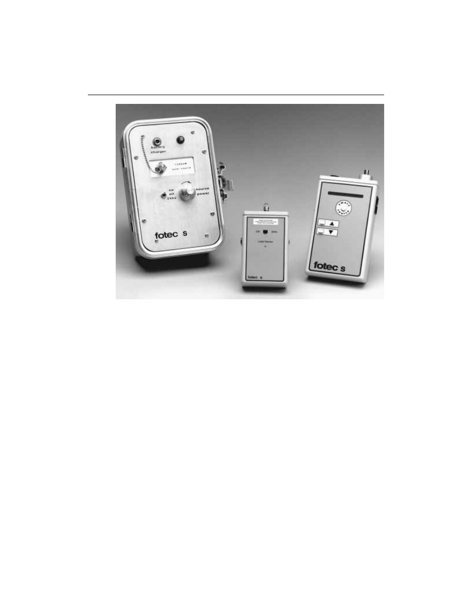
Figure 17-2

Fiber optic test sources. Courtesy Fotec, Inc.

type of fiber in use (singlemode or multimode, with the proper core diameter) and
the wavelength desired for performing the test. Most sources are either LEDs or
lasers of the types commonly used as transmitters in actual fiber optic systems,
making them representative of actual applications and enhancing the usefulness
of the testing.

Typical wavelengths of sources are 665 nm (plastic fiber), 850 nm (short

wavelength multimode glass fiber), and 1300 and 1550 nm (long wavelength
multimode and singlemode fiber). LEDs are typically used for testing multimode
fiber and lasers are used for singlemode fiber, except for the testing of short sin-
glemode jumper cables with LEDs. The broad spectral output of an LED has
higher attenuation in singlemode fiber than a laser, causing significant errors on
cables longer than about 5 kilometers. The source wavelength can be a critical
issue in making accurate loss measurements on longer cable runs, since attenua-
tion of the fiber is wavelength sensitive, especially at short wavelengths. Thus all
test sources should be calibrated for wavelength.

Adaptability to a variety of fiber optic connectors is important also, since

over 70 styles of connectors exist, although the types most commonly used are ST

182

CHAPTER 17 — FIBER OPTIC TESTING

and SC for multimode fiber and SC or FC for singlemode fiber. The new small
form factor connectors (LC, MT–RJ, VF–45) are also gaining in popularity.
Some LED sources use modular adapters such as power meters to allow adapta-
tion to various connector types. Lasers almost always have fixed connectors. If
the connector on the source is fixed, hybrid test jumpers with connectors com-
patible with the source on one end and the connector being tested on the other
must be used.

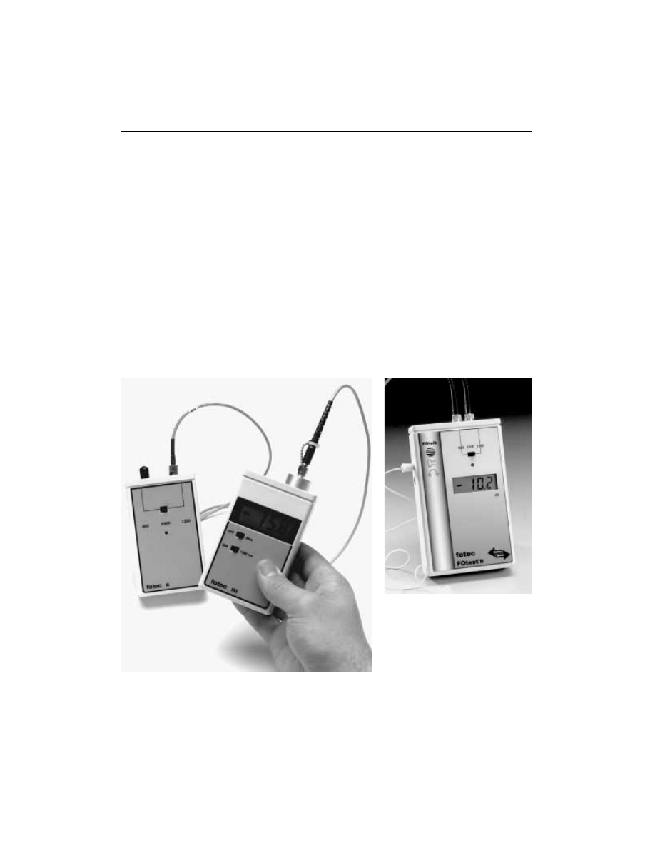
Optical Loss Test Sets/Test Kits

The optical loss test set (Figure 17-3) is an instrument formed by the combination
of a fiber optic power meter and source that is used to measure the loss of fiber,
connectors, and connectorized cables. Early versions of this instrument were
called attenuation meters. A test kit has a similar purpose, but is usually com-
prised of separate instruments and includes accessories to customize it for a spe-
cific application, such as testing a fiber optic LAN, telco, or CATV.

CHAPTER 17 — FIBER OPTIC TESTING

183

Figure 17-3

An optical loss

test set can be separate
source and power meter (a) or
an integrated single instrument
(b). Courtesy Fotec, Inc

(a)

(b)

The combination optical loss test set (OLTS) instrument may be useful for

making measurements in a laboratory, but in the field, individual sources and
power meters are more often used, since the ends of the fiber and cable are usu-
ally separated by long distances, which would require two OLTSs, at double the
cost of one fiber optic power meter and source. And even in a laboratory envi-
ronment, several different source types may be needed, making the flexibility of a
separate source and meter a better choice.

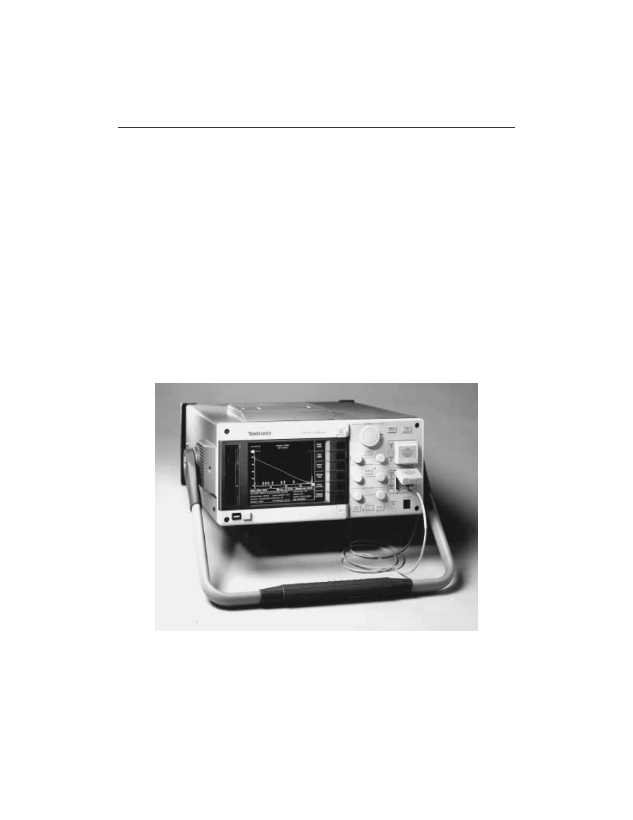
Optical Time Domain Reflectometers

The OTDR (Figure 17-4) uses the phenomenon of fiber backscattering to charac-
terize fibers, find faults, and optimize splices. Since scattering is one of the pri-
mary loss factors in fiber (the other being absorption), the OTDR can send out
into the fiber a high-powered pulse and measure the light scattered back toward
the instrument. The pulse is attenuated on the outbound leg and the backscat-
tered light is attenuated on the return leg, so the returned signal is a function of
twice the fiber loss and the backscatter coefficient of the fiber.

If one assumes the backscatter coefficient is constant, the OTDR can be used

to measure loss as well as to locate fiber breaks, splices, and connectors. In addi-

184

CHAPTER 17 — FIBER OPTIC TESTING

Figure 17-4a

Full featured OTDRs offer maximum range and flexibility.

Courtesy Tektronix

CHAPTER 17 — FIBER OPTIC TESTING

185

Figure 17-4b

Mini OTDRs offer fewer features in much smaller

packages and at less cost. Courtesy Photon-Kinetics, Inc.

Figure 17-4c

Fault finders are single OTDRs for troubleshooting.

Courtesy Tektronix

tion, the OTDR gives a graphic display of the status of the fiber being tested. And
it offers another major advantage over the source/fiber optic power meter or
OLTS in that it requires access to only one end of the fiber.

OTDRs generally are used to test all outside plant installations, especially to

confirm the loss of splices between lengths of cables. The distance resolution of a
typical OTDR, however, is too long to see the typical patch cords used in most
cable plants, limiting their usefulness for premises cabling installations. Also, all
network specifications call for testing the cables with a source and power meter,
as that tests the cables exactly as they will be used in the application.

The uncertainty of the OTDR measurement is heavily dependent on the

backscatter coefficient, which is a function of intrinsic fiber scattering character-
istics, core diameter, and numerical aperture. It is the variation in backscatter
coefficient that causes many splices to show a “gain” instead of the actual loss.
Tests have shown that OTDR splice loss measurements may have an uncertainty
of up to 0.8 dB. OTDRs must also be matched to the fibers being tested in both
wavelength and fiber core diameter to provide accurate measurements. Thus
many OTDRs have modular sources to allow substituting a proper source for the
application.

While most OTDR applications involve finding faults in installed cables or

optimizing splices, they are very useful in inspecting fibers for manufacturing
faults. Development work on improving the short-range resolution of OTDRs for
LAN applications and new applications such as evaluating connector return loss
promise to enhance the usefulness of the instrument in the future.

OTDRs come in three basic versions. Full-size OTDRs offer the highest per-

formance and have a full complement of features such as data storage, but are
very big and high priced. Mini OTDRs provide the same types of measurements
as a full OTDR, but with fewer features to trim the size and cost. Fault finders
use the OTDR technique, but are greatly simplified to provide just the distance to
a fault, to make the instruments more affordable and easier to use.

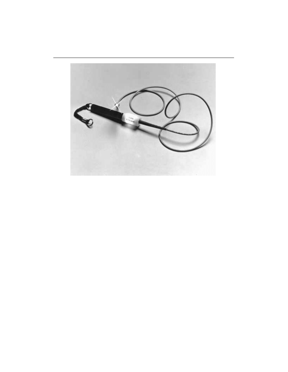
Visual Cable Tracers and Fault Locators

Many of the problems in fiber optic networks are related to making proper con-
nections. Since the light used in systems is invisible, one cannot see the system
transmitter light. By injecting the light from a visible source, such as an LED or
incandescent light bulb, one can visually trace the fiber from transmitter to
receiver to insure correct orientation and also to check continuity. The simple
instruments that inject visible light are called visual fault locators (Figure 17-5).

If a powerful enough visible light, such as an HeNe or visible diode laser, is

injected into the fiber, high loss points can be made visible. Most applications
center around short cables such as those used in telco central offices to connect to
the fiber optic trunk cables. However, since visible light covers the range where
OTDRs are not useful, it is complementary to the OTDR in cable troubleshoot-

186

CHAPTER 17 — FIBER OPTIC TESTING

ing. This method will work on buffered fiber and even jacketed single-fiber cable
if the jacket is not opaque to the visible light. The yellow jacket of singlemode
fiber and orange of multimode fiber will usually pass the visible light. Most other
colors, especially black and gray, will not work with this technique, nor will most
multifiber cables. However, many cable breaks, macrobending losses caused by
kinks in the fiber, bad splices, and so on can be detected visually. Since the loss in
the fiber is quite high at visible wavelengths, on the order of 9 to 15 dB/km, this
instrument has a short range, typically 3 to 5 kilometers.

Fiber Identifiers

If one carefully bends a singlemode fiber enough to cause loss, the light that cou-
ples out can also be detected by a large area detector. A fiber identifier uses this
technique to detect a signal in the fiber at normal transmission wavelengths.
These instruments usually function as receivers, able to discriminate between no
signal, a high speed signal, and a 2 kHz tone. By specifically looking for a 2 kHz
“tone” from a test source coupled into the fiber, the instrument can identify a
specific fiber in a large multifiber cable, especially useful to speed up the splicing
or restoration process.

CHAPTER 17 — FIBER OPTIC TESTING

187

Figure 17-5

A simple fiber tracer is a flashlight coupled to the fiber

optic cable. Courtesy Fotec, Inc.

Fiber identifiers can be used with both buffered fiber and jacketed single-

fiber cable. With buffered fiber, one must be very careful to not damage the fiber,
as any excess stress here could result in stress cracks in the fiber that could cause
a failure in the fiber anytime in the future.

Optical Continuous Wave Reflectometers

The optical continuous wave reflectometer (OCWR) was originally proposed as a
special purpose instrument to measure the optical return loss of singlemode con-
nectors installed on patch cords or jumpers. Unfortunately, its purpose became
muddled between conception and inception. As actual instruments came on the
market, they had much higher measurement resolution than appropriate for the
measurement uncertainty (0.01 dB resolution versus 1 dB uncertainty), leading to
much confusion on the part of users as to why measurements were not repro-
ducible. In addition, several instruments were touted as a way to measure the
optical return loss of an installed cable plant, obviously in ignorance of the fact
that they would also be integrating the backscatter of the fiber with any reflec-
tions from connectors or splices. Since the measurement of return loss from a
connector can be made equally well with any power meter, laser source, and cal-
ibrated coupler, and an OTDR is the only way to test installed cable plants for
return loss, the OCWR has little use in fiber optic testing.

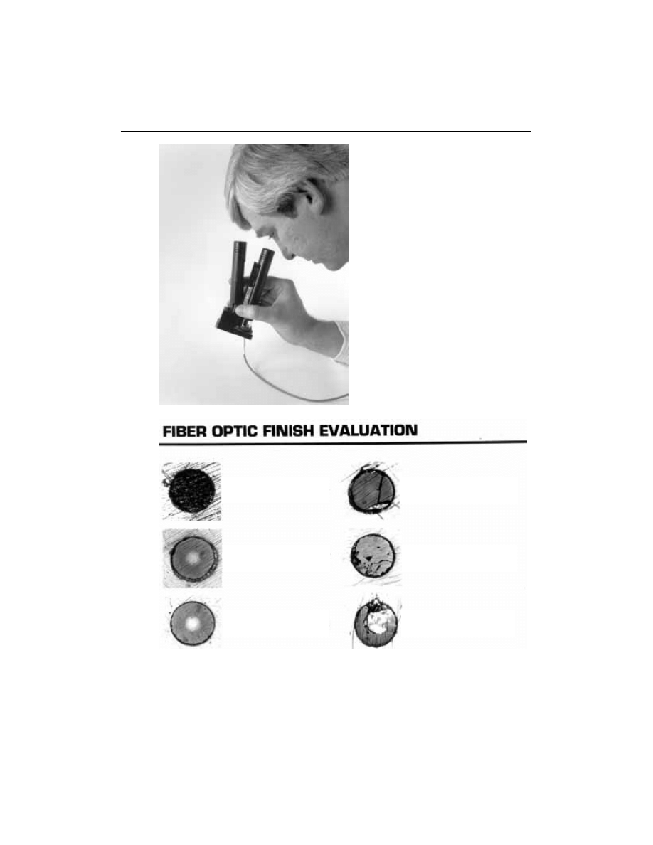
Visual Inspection with Microscopes

Cleaved fiber ends prepared for splicing and polished connector ferrules require
visual inspection to find possible defects. This is accomplished using a micro-
scope with a stage modified to hold the fiber or connector in the field of view
(Figure 17-6). Fiber optic inspection microscopes vary in magnification from 30
to 800 power, with 30 to 100 power being the most widely used range. Cleaved
fibers are usually viewed from the side, to see breakover and lip. Connectors are
viewed end-on or at a small angle to find polishing defects such as scratches (Fig-
ure 17-7).

Fiber Optic Talksets

Although technically not a measuring instrument, fiber optic talksets are some-
times used for fiber optic installation and testing. They transmit voice over fiber
optic cables already installed, allowing technicians splicing or testing the fiber to
communicate effectively. Talksets are especially useful when walkie-talkies and
cellular telephones are not available, such as in remote locations where splicing is
being done, or in buildings where radio waves will not penetrate.

Attenuators

Attenuators are used to simulate the loss of long fiber runs for testing link margin
in network simulation in the laboratory or self-testing links in a loopback config-

188

CHAPTER 17 — FIBER OPTIC TESTING

CHAPTER 17 — FIBER OPTIC TESTING

189

Figure 17-6

Microscopes allow

inspection of connectors for polish
quality, cleanliness, and faults.
Courtesy Fotec, Inc.

Figure 17-7

Connector faults are easily seen through a microscope. Courtesy

Buehler LTD

TYPICAL 3
MICRON FINISH AT 200X

TYPICAL 1
MICRON FINISH AT 200X

TYPICAL 0.3
MICRON FINISH AT 200X

CRACKED AND
CHIPPED FINISH AT 200X

PLUCKED
FINISH AT 200X

CRACKED AND
PLUCKED FINISH AT 200X

uration. In margin testing, variable attenuators are used to increase loss until the
system has a high bit error rate. For loopback testing, an attenuator is used
between a single piece of the equipment’s transmitter and receiver to test for
operation under maximum specified fiber loss. If systems work in loopback test-
ing, they should work with a proper cable plant. Thus, many manufacturers of
network equipment specify a loopback test as a diagnostic/troubleshooting pro-
cedure.

Attenuators can be made by gap loss, or a physical separation of the ends of

the fibers, inducing bending losses or inserting calibrated optical filters. Both
variable and fixed attenuators are available, but variable attenuators are usually
used for testing. Fixed attenuators may be inserted in the system cables where dis-
tances in the fiber optic link are too short and excess power at the receiver causes
transmission problems.

Test Jumper Cables and Bulkhead Splice Adapters

In order to test cables using the FOTP-171 insertion loss test, one needs to estab-
lish test conditions. This requires launch jumper cables to connect the test source
to the cable under test and receive cables to connect the fiber optic power meter.
For accurate measurements, the launch and receive cables must be made with
fiber and connectors matching the cables to be tested. To provide reliable mea-
surements, launch and receive cables must be in good condition. They can easily
be tested against each other to insure their performance. Bulkhead splices are
used to connect the cables under test to the launch and receive cables. Only the
highest performance bulkhead splices should be used, and their condition
checked regularly, since they are vitally important in obtaining low loss connec-
tions.

OPTICAL POWER

The most basic fiber optic measurement is optical power from the end of a fiber.
This measurement is the basis for loss measurements as well as the power from a
source or at a receiver. Although optical power meters are the primary measure-
ment instrument, OLTSs and OTDRs also measure power differences in testing
loss. EIA standard test FOTP-95 covers the measurement of optical power.

Optical power is based on the heating power of the light, and some instru-

ments actually measure the heat when light is absorbed in a detector. While this
may work for high-powered lasers, these detectors are not sensitive enough for
the power levels typical for fiber optic communication systems. Table 17-2 shows
typical power levels in fiber optic systems.

Optical power meters typically use semiconductor detectors since they are

extremely sensitive to light in the wavelengths common to fiber optics (Table 17-3).
Most fiber optic power meters are available with a choice of three different detec-

190

CHAPTER 17 — FIBER OPTIC TESTING

tors, silicon (Si), Germanium (Ge), or Indium-Gallium-Arsenide (InGaAs). Silicon
photodiodes are sensitive to light in the range of 400 to 1000 nm and germanium
and indium-gallium-arsenide photodiodes are sensitive to light in the range of
800 to 1600 nm.

Calibration

Calibrating fiber optic power measurement equipment requires setting up a refer-
ence standard traceable to national standards laboratories such as the NIST.
Fiber optic power meters have an uncertainty of calibration of about ±5%, com-
pared to NIST primary standards. Limitations in the uncertainty are the inherent
inconsistencies in optical coupling, about 1 percent at every transfer, and slight
variations in wavelength calibration. NIST is working continuously with instru-
ment manufacturers and private calibration labs to try to reduce the uncertainty
of these calibrations.

NIST offers fiber optic power calibration services at 850-nm, 1300-nm, and

1550-nm wavelengths, so most fiber optic power meters offer calibrations at
those wavelengths. Fiber optic networks may work at slightly different wave-
lengths than those calibration wavelengths. For example multimode LED net-
works use LEDs that are referred to as 1300 nm but have broad spectral outputs,
and singlemode networks use lasers referred to as 1310-nm wavelength but

CHAPTER 17 — FIBER OPTIC TESTING

191

Table 17-2

Optical Power Levels of Fiber Optic Communication Systems

Network Type

Wavelength (nm)

Power Range (dBm)

Power Range (W)

Telecom

1310, 1550

+3 to –45

50 nW to 2mW

Datacom

665, 790, 850,

–10 to –30

1 to 100uW

1300

CATV

1310, 1550

+10 to –6

250uW to 10mW

Table 17-3

Characteristics of Detectors Used in Fiber Optic Power Meters

Detector Type

Wavelength Range (nm)

Power Range (dBm)

Comments

Silicon

400–1100

+10 to –70

Germanium

800–1600

+10 to –60

–70 with small area
detectors, +30 with
attenuator windows

Indium-

800–1600

+10 to –70

Small area detectors may

Gallium-

overload at high power

Arsenide

(>.0 dBm)

actually vary between 1290 and 1330 nm. Since the difference in calibration
between 1300 and 1310 nm is insignificant and the actual devices vary from that
wavelength significantly, measurements are made only to those calibration wave-
lengths. Networks using 790-nm transmitters are usually tested at 850-nm cali-
bration, and plastic optical fiber is tested with meters calibrated at 650 nm
traceable to other NIST optical power standards.

Recalibration of instruments should be done annually; however, experience

has shown that the accuracy of meters rarely changes significantly during that
period, as long as the electronics of the meter do not fail. Unfortunately, the cali-
bration of fiber optic power meters requires considerable investment in capital
equipment and continual updating of the transfer standards, so very few private
calibration labs exist today. Most meters must be returned to the original manu-
facturer for calibration.

Instrument Resolution versus Measurement Uncertainty

The uncertainty of optical power measurements is about 0.2 dB (5 percent). Loss
measurements are likely to have uncertainties of 0.5 dB or more, and optical
return loss measurements have about 1 dB uncertainty. Instruments with read-
outs with a resolution of 0.01 dB are generally only appropriate for laboratory
measurements of very low losses such as connectors or splices under 1 dB or for
monitoring small changes in loss of power over environmental changes.

Field instruments are better when the instrument resolution is limited to 0.1

dB, since the readings will be less likely to be unstable when being read and more
indicative of the measurement uncertainty. This is especially important since field
personnel are usually not as well trained in the nuances of measurement uncer-
tainty.

OPTICAL FIBER TESTING

The installer rarely tests fiber or cable before it is installed and terminated except
to perform a continuity test before installation to insure no damage has been
done to the cable during shipment to the work site. Manufacturers of fiber and
cable have already tested the fibers thoroughly and usually provide extensive test
data along with the cable.

Continuity Testing

Continuity testing is the most fundamental fiber optic test. It is usually performed
with a visible light source, which can be an incandescent light bulb, HeNe laser at
633 nm, or a LED or diode laser at 650 nm, readily seen by the eye. HeNe laser
instruments are usually tuned to an output power level of just less than 1 mW,
making them Class II lasers, which do not have enough power to harm the eye,

192

CHAPTER 17 — FIBER OPTIC TESTING

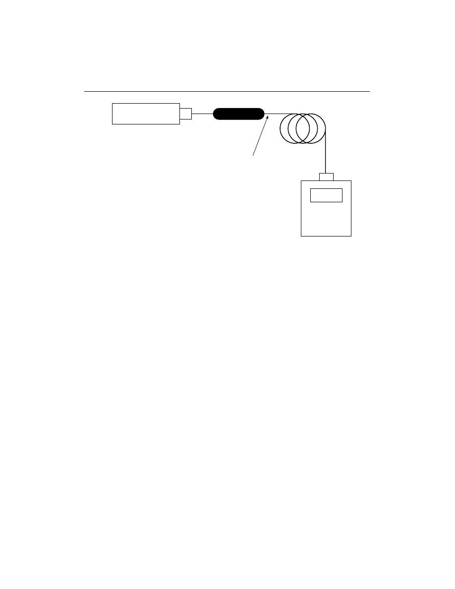
Figure 17-8

Fiber attenuation by cutback method.

but do have enough power to be seen easily over about 4 kilometers of fiber, and
even find fiber microbends or breaks by viewing the light shining from the break
through the yellow or orange jacket used on most single fiber cables.

Testing Fiber Attenuation

Measuring the fiber attenuation coefficient requires transmitting light of a known
wavelength through the fiber and measuring the changes over distance. The con-
ventional method, known as the cutback method (Figure 17-8), involves coupling
fiber to the source and measuring the power out of the far end. The fiber is then
cut near the source and power measured again. By knowing the power at the
source and end of the fiber and the length of the fiber, its attenuation coefficient
can be determined by calculating:

(P

end

– P

source

) (dB)

attenuation coefficient (dB) = ————————

length(km)

An alternative method of testing fiber, which may be easier in field measure-

ments, involves attaching a fiber pigtail to the source that has a connector on one
end and a temporary splice on the other end, similar to the loss measurement of
terminated cables. This method introduces more uncertainty in the measurement
because of the loss of the splice coupled to the fiber under test, since it may not be
easy to accurately calibrate the output power of the pigtail. The best method is to

CHAPTER 17 — FIBER OPTIC TESTING

193

Source

–3.1

Power

Meter

Fiber to Test

Modal Conditioning

Cutback to Here

use a bare fiber adapter on the power meter to measure the output of the bare
fiber, then attach the splice. Alternately, have the splice attached on the pigtail
and couple a large core fiber to the pigtail with the splice and measure the power.
The large core fiber will minimize losses in the splice for accurate calibration.

Sources for Loss Measurements

For loss measurements the source can be a fixed-wavelength LED or laser,
whichever is appropriate to the fiber being tested. Most multimode fiber systems
use LED sources, whereas singlemode fiber systems use laser sources. Thus, test-
ing each of these fibers should be done with the appropriate source. Lasers gener-
ally should not be used with multimode fiber, since coherent sources such as
lasers have high measurement uncertainties in multimode fiber caused by modal
noise. Networks like gigabit Ethernet are too fast for LED sources, so they use
lasers and special launch conditions to reduce modal noise. The cable may show
significantly lower loss with a laser source than an LED due to different modal
conditions. In this circumstance, testing with a source similar to a system source
will give more accurate results.

LEDs can be used to test short singlemode cables. However, the wide spectral

width of LEDs sometimes overlaps the singlemode fiber cutoff wavelength (the
lowest wavelength where the fiber supports only one mode) at lower wavelengths
and the 1400-nm hydroxide radical (/OH+): absorption band at the upper wave-
lengths, creating errors in loss measurements on longer singlemode cables (over
about 5 km).

Modal Effects on Attenuation

In order to test multimode fiber optic cables accurately and reproducibly, it is
necessary to understand modal distribution, mode control, and attenuation cor-
rection factors. Modal distribution in multimode fiber is very important to mea-
surement reproducibility and accuracy. For most field tests, using a source similar
to the system source will minimize errors.

Mode Conditioners

There are three basic “gadgets” to condition the modal distribution in multimode
fibers (Figure 17-9): mode strippers that remove unwanted cladding mode light,
mode scramblers that mix modes to equalize power in all the modes, and mode
filters that remove the higher order modes to simulate equilibrium modal distrib-
ution (EMD) or steady state conditions. These devices have been described in
detail in many articles on testing but are not commonly used in field measure-
ments today, due to the standardization of most link components.

194

CHAPTER 17 — FIBER OPTIC TESTING

Figure 17-9

Mode conditioners for multimode graded-index fibers.

Modal Effects in Testing Singlemode Fiber

Testing singlemode fiber is easy compared to multimode fiber. Singlemode fiber,
as the name says, only supports one mode of transmission for wavelengths
greater than the cutoff wavelength of the fiber. Thus, most problems associated
with mode power distribution are no longer a factor. However, it takes a short
distance for singlemode fiber to really be singlemode, since several modes may be
supported for a short distance after connectors, splices, or sources. Singlemode
fibers shorter than 10 meters may have several modes. To insure short cables
have only one mode of propagation, one can use a simple mode filter made from
a 4- to-6 inch loop of the cable.

CHAPTER 17 — FIBER OPTIC TESTING

195

Fiber

Buffer

Mode Stripper

Mode Scrambler

Index-Matching Material

Splice

Splice

Graded Index

Step Index

Graded Index

Mode Filter

Fiber

Mandrel

Bending Losses

Fiber and cable are subject to additional losses as a result of stress. In fact, fiber
makes a very good stress sensor. However, this is an additional source of uncer-
tainty when making attenuation measurements. It is mandatory to minimize
stress and/or stress changes on the fiber when making measurements. If the fiber
or cable is spooled, it will have higher loss when spooled tightly. It may be advis-
able to unspool it and respool with less tension. Unspooled fiber should be care-
fully placed on a bench and taped down to prevent movement. Above all, be
careful about how connectorized fiber is placed. Dangling fibers that stress the
back of the connector will have significant losses.

Transmission versus OTDR Tests

So far, we have only discussed testing attenuation by transmission of light from a
source, but one can also imply fiber losses by backscattered light from a source
using an OTDR.

OTDRs are widely used for testing fiber optic cables. Among the common

uses are measuring the length of fibers, and finding faults in fibers, breaks in
cables, attenuation of fibers, and losses in splices and connectors. They are also
used to optimize splices by monitoring splice loss. One of their biggest advan-
tages is that they produce a picture (called a trace) of the cable being tested.
Although OTDRs are unquestionably useful for all these tasks, they have error
mechanisms that are potentially large, troublesome, and not widely understood.

OTDR Operation

The OTDR (Figure 17-10) uses the lost light scattered in the fiber that is directed
back to the source for its operation. It couples a pulse from a high-powered laser
source into the fiber through a directional coupler. As the pulse of light passes
through the fiber, a small fraction of the light is scattered back toward the source.
As it returns to the OTDR, it is directed by the coupler to a very sensitive
receiver. The OTDR display (Figure 17-11) shows the intensity of the returned
signal in dB as a function of time, converted into distance using the average veloc-
ity of light in the glass fiber.

To understand how the OTDR allows measurement, consider what happens

to the light pulse it transmits. As it goes down the fiber, the pulse actually “fills”
the core of the fiber with light for a distance equal to the pulse width transmitted
by the OTDR. In a typical fiber, each nanosecond of pulse width equals about 8
inches (200 mm). Throughout that pulse, light is being scattered, so the longer
the pulse width in time, the greater the pulse length in the fiber, the greater will be
the amount of backscattered light, in direct proportion to the pulse width. The
intensity of the pulse is diminished by the attenuation of the fiber as it proceeds

196

CHAPTER 17 — FIBER OPTIC TESTING

Figure 17-10

An OTDR block diagram.

Figure 17-11

OTDR display.

down the fiber, a portion of the pulse’s power is scattered back to the OTDR and
it is again diminished by the attenuation of the fiber as it returns up the fiber to
the OTDR. Thus, the intensity of the signal seen by the OTDR at any point in
time is a function of the position of the light pulse in the fiber.

CHAPTER 17 — FIBER OPTIC TESTING

197

Laser

Coupler

Receiver

Boxcar

Averager

Fiber to

Test

Display

Laser Pulse

Splice

Back Reflection

End of Fiber

Distance

dB

Connector

By looking at the reduction in returned signal over time, one can calculate the

attenuation coefficient of the fiber being tested. Since the pulse travels out and
back, the attenuation of the fiber diminishes the signal in both directions, and the
transit time from pulse out to return is twice the one-way travel time. So both the
intensity and distance scales must be divided by two to allow for the round-trip
path of the light.

If the fiber has a splice or connector, the signal will be diminished as the pulse

passes it, so the OTDR sees a reduction in power, indicating the light loss of the
joined fibers. If the splice or connector reflects light (see optical return loss), the
OTDR will show the reflection as a spike above the backscattered signal. The
OTDR can be calibrated to use this spike to measure optical return loss.

The end of the fiber will show as a deterioration of the backscatter signal into

noise if it is within the dynamic range of the OTDR. If the end of the fiber is
cleaved or polished, one will also see a spike above the backscatter trace. This
allows one to measure the total length of the fiber being tested.

In order to enhance the signal to noise ratio of the received signal, the OTDR

sends out many pulses and averages the returned signals. And to get to longer dis-
tances, the power in the transmitted pulse is increased by widening the pulse
width. The longer pulse width fills a longer distance in the fiber as noted earlier.
This longer pulse width masks all details within the length of the pulse, increasing
the minimum distance between features resolvable with the OTDR.

OTDR Measurement Uncertainties

With the OTDR, one can measure loss and distance. To use them effectively, it is
necessary to understand their measurement limitations. The OTDR’s distance
resolution is limited by the transmitted pulse width. As the OTDR sends out its
pulse, crosstalk in the coupler inside the instrument and reflections from the first
connector will saturate the receiver. The receiver will take some time to recover,
causing a nonlinearity in the baseline of the display. It may take 100 to 1,000
meters before the receiver recovers. It is common to use a long fiber cable called
a pulse suppresser between the OTDR and the cables being tested to allow the
receiver to recover completely.

The OTDR also is limited in its ability to resolve two closely spaced features

by the pulse width. Long distance OTDRs may have a minimum resolution of
250 to 500 meters, while short range OTDRs can resolve features 5 to 10 meters
apart. This limitation makes it difficult to find problems inside a building, where
distances are short. A visual fault locator is generally used to assist the OTDR in
this situation.

When measuring distance, the OTDR has two major sources of error not

associated with the instrument itself: the velocity of the light pulse in the fiber and
the amount of fiber in the cable. The velocity of the pulse down the fiber is a

198

CHAPTER 17 — FIBER OPTIC TESTING

CHAPTER 17 — FIBER OPTIC TESTING

199

function of the average index of refraction of the glass. While this is fairly constant
for most fiber types, it can vary by a few percent. When making cable, it is neces-
sary to have some excess fiber in the cable, to allow the cable to stretch when
pulled without stressing the fiber. This excess fiber is usually 1 to 2 percent. Since
the OTDR measures the length of the fiber, not the cable, it is necessary to sub-
tract 1 to 2 percent from the measured length to get the likely cable length. This is
very important if one is using the OTDR to find a fault in an installed cable, to
keep from looking too far away from the OTDR to find the problem. This vari-
able adds up to 10 to 20 meters per kilometer, therefore it is not ignorable.

When making loss measurements, two major questions arise with OTDR

measurement anomalies: why OTDR measurements differ from an OLTS, which
tests the fiber in the same configuration in which it is used, and why measure-
ments from OTDRs vary so much when measured in opposite directions on the
same splice. And why one direction sometimes shows a gain, not a loss.

In order to understand the problem, it is necessary to consider again how

OTDRs work (Figure 17-12). They send a powerful laser pulse down the fiber,
which suffers attenuation as it proceeds. At every point on the fiber, part of the
light is scattered back up the fiber. The backscattered light is then attenuated by
the fiber again, until it returns to the OTDR and is measured.

Note that three factors affect the measured signal: attenuation outbound,

scattering, and attenuation inbound.

It is commonly assumed that the backscatter coefficient is a constant, and

therefore the OTDR can be calibrated to read attenuation. The backscatter coef-
ficient is, in fact, a function of the core diameter of the fiber (or mode field diam-
eter in singlemode fiber) and the material composition of the fiber (which
determines attenuation). Thus, a fiber with either higher attenuation or larger
core size will produce a larger backscatter signal.

Accurate OTDR attenuation measurements depend on having a constant

backscatter coefficient. Unfortunately, this often is not the case. Fibers with
tapers in core size are common, or variations in diameter as the result of varia-
tions in pulling speed as the fiber is being made. A small change in diameter (1
percent) causes a larger change in cross-sectional area that directly affects the
scattering coefficient and can cause a large change in attenuation (on the order of
0.1 dB). Thus, fiber attenuation measured by OTDRs may be nonlinear along the
fiber and produce significantly different losses in opposite directions.

The first indication of OTDR problems for most users occurs when looking

at a splice and a gain is seen at the splice. Common sense tells us that passive
fibers and splices cannot create light, so another phenomenon must be at work.
In fact, a “gainer” is an indication of the difference of backscatter coefficients in
the two fibers being spliced.

If an OTDR is used to measure the loss of a splice and the two fibers are

identical, the loss will be correct, since the scattering coefficient is the same for

200

CHAPTER 17 — FIBER OPTIC TESTING

Backscatter

Test Pulse

Fiber A

Backscatter

Test Pulse

Fiber B

Loss

Actual Splice Loss

}

(a)

(b) Fiber A = Fiber B

Actual

}

Variation Caused by
Difference in Scattering
Coefficient

}

Actual Splice Loss

}

Variation Caused by Difference
in Scattering Coefficient

}

(c) Loss A > Loss B

(d) Loss A < Loss B (“Gainer”)

Splice

Figure 17-12

OTDR loss measurement uncertainty.

both fibers. This is exactly what you see when breaking and splicing the same
fiber, the normal way OTDRs are demonstrated.

If the receiving fiber has a lower backscatter coefficient than the fiber before

the splice, the amount of light sent back to the OTDR will decrease after the
splice, causing the OTDR to indicate a larger splice loss than actual.

If one looks at this splice in the opposite direction, the effect will be reversed.

The amount of backscattered light will be larger after the splice and the loss
shown on the OTDR will be less than the actual splice loss. If this increase is
larger than the loss in the splice, the OTDR will show a gain at the splice, an
obvious error. As many as one-third of all splices will show a gain in one direc-
tion.

The usual recommendation is to test with the OTDR in both directions and

average the reading, which has been shown to give measurements accurate to
about 0.01 dB. But this negates the most useful feature of the OTDR, the ability
to work from only one end of the fiber. And all network specifications call for
loss testing with a source and meter, which must be done also.

Bandwidth Testing

Fiber’s information transmission capacity is limited by two separate components
of dispersion: modal and chromatic. Modal dispersion occurs in step-index mul-
timode fiber where the paths of different modes are of varying lengths. Modal
dispersion also comes from the fact that the index profile of graded-index (GI)
multimode fiber is not perfect.

The second factor in fiber bandwidth is chromatic dispersion. Remember, a

prism spreads out the spectrum of incident light, since the light travels at different
speeds according to its color and is therefore refracted at different angles. The
usual way of stating this is the index of refraction of the glass is wavelength
dependent. Thus, a carefully manufactured graded-index multimode fiber can
only be optimized for a single wavelength, usually near 1300 nm, and light of
other colors will suffer from chromatic dispersion. Even light in the same mode
will be dispersed if it is of different wavelengths.

Chromatic dispersion is a bigger problem with LEDs, which have broad spec-

tral outputs, unlike lasers that concentrate most of their light in a narrow spectral
range. Chromatic dispersion occurs with LEDs because much of the power is
away from the zero dispersion wavelength of the fiber. High speed systems such
as FDDI, based on broad output surface emitter LEDs, suffer such intense chro-
matic dispersion that transmission over only 2 to 3 km of 62.5/125 fiber can be
risky.

Modal dispersion is the most commonly tested bandwidth factor. Testing is

done by using a narrow spectral width laser source and high-speed receiver to
determine dynamic characteristics. Testing can be done by sweeping the frequency

CHAPTER 17 — FIBER OPTIC TESTING

201

of a sine wave and looking for attenuation in the pulse peak height, which leads to
a specification of bandwidth at the 3 dB loss point, that is, pulse height is 0.5 the
value at low frequency. The alternate method is to measure degradation of pulse
risetime.

Chromatic dispersion requires comparing pulse transit times or phase shift as

a function of wavelength. Thus, sources of several wavelengths are used and vari-
ations in time allow calculating dispersion as a function of wavelength. Although
it seems that this could be done with a broad spectral width source such as an
LED, the removal of the effects of the spectral characteristics of the LED is very
complicated mathematically and every LED is unique in its spectral characteris-
tics, making calibration of test equipment very difficult.

Since all this test equipment must work in the GHz range, it is very expen-

sive. Fortunately, fiber bandwidth characteristics have been very well modeled
and the characteristics calculated with precision comparable to actual measure-
ments. There have been at least two models described in detail and one available
commercially. The one available commercially (Fotec’s Cable Characterizer) cal-
culates bandwidth for multimode fibers based on inputs of fiber modal band-
width and length and source wavelength and spectral width.

Using the models one can easily determine if the installed fiber is adequate

for higher-speed networks such as FDDI. They can help designers design net-
works with adequate bandwidth for high-speed networks without spending too
much on overspecified fiber, and provide a way for the installer or end user to
certify cable plants for FDDI and other high-speed networks.

CONNECTOR AND SPLICE LOSS TESTING

Connector loss is the major cause of loss in short fiber optic cable plant runs,
making it a very important measurement. Most cable testing is done after the
connectors are installed, so the loss includes the connectors. Splice testing is more
complicated. Expensive fusion splicers estimate the splice loss themselves, and the
data is quite reliable. Splice testing is generally done with an OTDR in both direc-
tions and averaged, but the cost and difficulty of splice testing is such that it usu-
ally is not done unless the splice quality is suspected from the total end-to-end
loss of the cable.

Connectors and splices are tested by the manufacturer to establish a typical

loss that can be expected by the experienced user. However, the actual loss of a
connector or splice is primarily a function of the installation process, not the
component itself. The connector itself is made very precisely, so the loss is deter-
mined by how well it is assembled and polished. Splice loss also depends on the
skill of the installer, although much less so than on the connector, since polishing

202

CHAPTER 17 — FIBER OPTIC TESTING

Figure 17-13

Connector insertion loss test.

is not needed. Large variations in loss from the manufacturer’s specifications for
loss may mean that the installer needs to improve either the installation process
or the test process.

In order to establish a typical loss for connectors or splices, it is necessary to

test them in a standardized fashion to allow for comparisons among various con-
nectors. Measurements of connector or splice losses are performed by measuring
the transmitted power of a short length of cable and then inserting a connector
pair or splice into the fiber (Figure 17-13). This test (designated FOTP-34 by the
EIA) can be used for both multimode and singlemode fiber, but the results for
multimode fiber are dependent on mode power distribution.

FOTP-34 has three options in modal distribution: (1) EMD or steady state,

(2) fully filled, and (3) any other conditions as long as they are specified. Besides
mode power distribution factors, the uncertainty of the measured loss is a combi-
nation of inherent fiber geometry variations, installed connector characteristics,
and the effects of the splice bushing used to align the two connectors.

This test is repeated hundreds or thousands of times by each connector man-

ufacturer to produce data that is quoted as an average value for the connector.
This shows the repeatability of their connector design, a critical factor in figuring
margins for installations using many connectors. Thus, loss is not the only crite-
rion for a good connector—it must be repeatable, so its average loss can be used
for these margin calculations with some degree of confidence.

CHAPTER 17 — FIBER OPTIC TESTING

203

Source

–3.1

Power

Meter

Fiber to Test

Modal Conditioning

Insert Connector

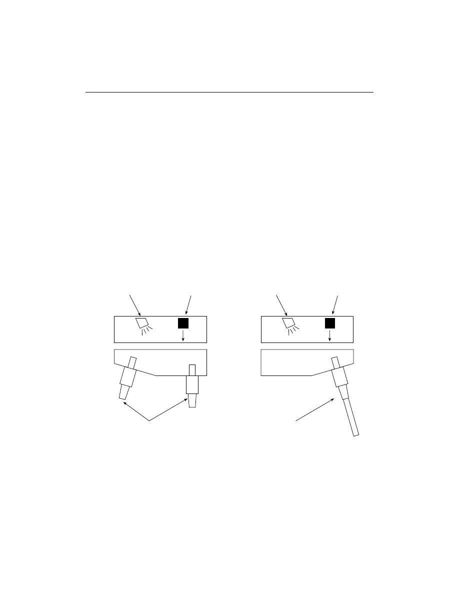
Figure 17-14

Inspecting connection with microscope.

Inspecting Connectors

Inspecting connectors in operating fiber optic links can be very dangerous if high
power levels are present, for instance from a laser source. Whenever inspecting
connectors in an installed or operating system, always check the connector with a
power meter to ensure no power is present.

Visual inspection of the end surface of a connector with a microscope is one

of the best ways to determine the quality of the termination procedure and diag-
nose problems. A well-made connector will have a smooth, polished, scratch-free
finish, and the fiber will not show any signs of cracks or pistoning (where the
fiber is either protruding from the end of the ferrule or pulling back into it).

The proper magnification for viewing connectors can be 30 to 400 power.

Lower magnification, typical with a jeweler’s loupe or pocket magnifier, will not
provide adequate resolution for judging the finish on the connector. Too high a
magnification tends to make small, ignorable faults look worse than they really
are. A better solution is to use medium magnification, but inspect the connector
three ways: viewing directly at the end of the polished surface with side lighting,
viewing directly with side lighting and light transmitted through the core, and
viewing at an angle with lighting from the opposite angle (Figure 17-14).

204

CHAPTER 17 — FIBER OPTIC TESTING

Light Bulb

Microscope Lens

Connector(s)

Light Bulb

Microscope Lens

Connector

Direct View with Core

Illumination

Angle View

Viewing directly with side lighting allows one to determine if the ferrule hole

is of the proper size, the fiber is centered in the hole, and a proper amount of
adhesive has been applied. Only the largest scratches will be visible this way,
however. Adding light transmitted through the core will make cracks in the end
of the fiber, caused by pressure or heat during the polish process, visible.

Viewing the end of the connector at an angle, while lighting it from the oppo-

site side at approximately the same angle, will allow the best inspection for the
quality of polish and possible scratches. The shadowing effect of angular viewing
enhances the contrast of scratches against the mirror-smooth polished surface of
the glass.

One needs to be careful in inspecting connectors, however. The tendency is

to be overly critical, especially at high magnification. Only defects over the fiber
core are a problem. Chipping of the glass around the outside of the cladding is
not unusual and will have no effect on the ability of the connector to couple light
in the core. Likewise, scratches only on the cladding will not cause any loss
problems.

An alternative way of viewing connector end faces is an interferometer. The

interferometer uses a special technique to show a profile of the end of the con-
nector that can determine its flatness or proper curvature for physical contact
(PC) connectors. Interferometers are important tools to use for critical connectors
such as PC singlemode types, but their size and cost limit their use to manufac-
turing facilities.

Optical Return Loss in Connectors

If you have ever looked at a fiber optic connector on an OTDR, you are familiar
with the characteristic spike that shows where the connector is. That spike is a
measure of the back reflection of optical return loss (ORL) of the connector, or
the amount of light that is reflected back up the fiber by light reflecting off the
interface of the polished end surface of the connector and air. It is called fresnel
reflection and is caused by the light going through the change in index of refrac-
tion at the interface between the fiber (n = 1.5) and air (n = 1).

For most systems, that return spike is just one component of the connector’s

loss, representing about 0.3 dB loss (two air/glass interfaces at 4 percent reflec-
tion each), the minimum loss for noncontacting connectors without index-match-
ing fluid. But in high bit-rate singlemode systems, that reflection can be a major
source of bit error-rate problems. The reflected light interferes with the laser
diode chip, causes mode-hopping, and can be a source of noise. Minimizing the
light reflected back into the laser is necessary to get maximum performance out
of high bit-rate laser systems, especially the analog modulation (AM) modulated
CATV systems.

CHAPTER 17 — FIBER OPTIC TESTING

205

State-of-the-art connectors will have a return loss of about 40 to 60 dB. Mea-

suring this back reflection can be done in the field with most of today’s OTDRs
or using a source and power meter per standard test procedure EIA FOTP-107 in
the manufacturing process. Generally, ORL is not measured in the field.

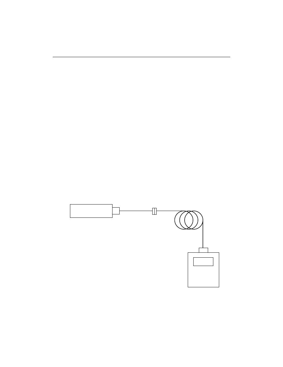
Connectorized Cable Testing

After connectors are added to a cable, testing must include the loss of the fiber in
the cable plus the loss of the connectors. This is the test that is most often per-
formed in the field after cable installation and termination. On very short cable
assemblies (up to 10 m long), the loss of the connectors will be the only relevant
loss, while fiber will contribute to the overall losses in longer cable assemblies. In
an installed cable plant, one must test the entire cable from end to end, including
every component in it, such as splices, couplers, and connectors intermediate
patch panels.

In testing connectorized cables, one uses a source with a launch cable attached

to calibrate the power being launched into the cable under test and a meter to
measure the loss. This test, FOTP-171, was developed along the lines of FOTP-34
for connectors (Figure 17-15). One begins by attaching to the source a launch
cable made from the same size fiber and connector type as the cables to be tested.
The power from the end of this launch cable is measured by a power meter to cal-
ibrate the launch power for the test. Then the cable to test is attached and power
measured at the end again. One can calculate the loss incurred in the connectors
mating to the launch cable and in the fiber in the cable itself.

206

CHAPTER 17 — FIBER OPTIC TESTING

Figure 17-15

Basic fiber optic cable loss test.

Source

–3.1

Power

Meter

Cable to Test

Launch

Cable

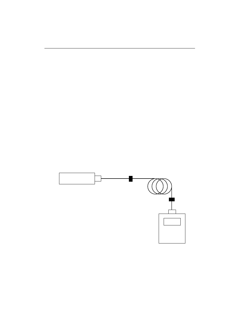
Since this only measures the loss in the connector mated to the launch cable,

one can add a second cable at the power meter end, called a receive cable, so the
cable to test is between the launch and receive cables. Then one measures the loss
at both connectors and in everything in between. This is commonly called a dou-
ble-ended loss test (Figure 17-16).

To obtain accurate loss measurements, it is important to calibrate the

launched power from the test source correctly. There have been two interpreta-
tions of the calibration of the output of the source in this test. One interpretation
(the incorrect one) is that one attaches the launch cable to the source and the
receive cable to the meter. The two are then mated and this becomes the “0 dB”
reference. The second method only attaches the launch cable to the source and
measures the power from the launch cable with the power meter.

With the first method, usually called the “two-cable reference,” one has two

new measurement uncertainties. First, this method underestimates the loss of the
cable plant by the loss of one connection, since that is zeroed out in the calibra-
tion process. Secondly, if one has a bad connector on one or both of the test
cables, it is hidden by the calibration, since even if the two connectors have a loss
of 10 dB, it is not seen by the calibration method used. This can lead to large
measurement errors, where losses measured will be higher than actual losses.

In the correct “single-cable” method, the launch power from the cable

attached to the source is measured directly by the power meter. This also allows
one to measure both connectors on the test cable, since power is referenced to the
output power of the launch connector. In addition, one can test the mating quality

CHAPTER 17 — FIBER OPTIC TESTING

207

Figure 17-16

Double-ended cable loss test.

Source

–3.1

Power

Meter

Cable to Test

Launch

Cable

Receive Cable

of the test cables’ connectors by attaching the receive jumper to the meter and then
measuring the loss of the connection between the launch and receive jumpers. If
this loss is high, one knows there is a problem with the test connectors that must
be fixed before actual cable loss measurements should be made.

Obviously, the second method is the proper method. Both methods are

detailed in OFSTP-14, the extension of FOTP-171 to include installed cable plants,
which also discusses the problems associated with mode power distribution. Also,
the loss specifications for the cable plant in all network specifications are written to
require that the single-cable launch power calibration method be used.

Finding Bad Connectors

If a test shows a jumper cable to have high loss, there are several ways to find the
problem. If you have a microscope, inspect the connectors for obvious defects
such as scratches, cracks, or surface contamination. If they look okay, clean them
before retesting. Retest the launch cable to make certain it is good. Then retest the
jumper cable with the single-ended method, using only a launch cable. Test the cable
in both directions. The cable should have higher loss when tested with the bad
connector attached to the launch cable, since the large area detector of the power
meter will not be affected as much by the typical loss factors of connectors.

Measuring Installed Splice Loss

Most fusion splicers have built-in equipment to inject and detect light transmitted
through the splice being made for estimating splice loss. These machines do not
require any other means of measuring splice loss. However, for other splice types,
it may be desirable to measure splice loss directly.

An OTDR can be used to measure splice loss, but its measurement uncer-

tainty caused by the different characteristics of the two different fibers used make
it more of a relative loss measurement than an absolute loss value. However, if
knowing the absolute loss of a splice is necessary, measure it with an OTDR in
both directions and average the results.

One can also measure the loss of a splice using a technique similar to the

FOTP-171 test for connectors. In order to measure the output to the launch fiber
(the one connected to the transmitter or test source), one must use a bare fiber
adapter on the power meter. After cleaving the fiber, measure the power with the
meter and use that as a reference. Once the fiber has been spliced, measuring the
loss, including the loss of the length of cable spliced on, can be done at the far end
of the fiber being spliced, which may be miles away. Since many splices are usu-
ally done at once, moving the power meter to the remote location each time is
impractical, so one needs another person with a calibrated meter at the remote
location to measure the power and report back the reading to allow calculation
of the loss.

208

CHAPTER 17 — FIBER OPTIC TESTING

Mode Power Distribution Effects on Loss in Multimode Fiber Cables

The biggest factor in the uncertainty of multimode cable loss tests is the mode
power distribution caused by the test source. When testing a simple 1 m cable
assembly, variations in sources can cause 0.3 to 1 dB variations in measured loss.
The effect is similar to the effect on fiber loss discussed earlier, since the concen-
tration of light in the lower order modes as a result of EMD or mode filtering will
minimize the effects of gap, offset, and angularity on mating loss by effectively
reducing the fiber core size and numerical aperture.

Although one can make mode scramblers and filters to control mode power

distribution when testing in the laboratory, it is more difficult to use these in the
field. The best way to get reliable measurements is to insure the test source uses a
source similar to a system source, not a controlled or restricted launch power dis-
tribution. An alternative technique is to use a special mode conditioning cable
between the source and launch cable that induces the proper mode power distri-
bution. This can be done with a step-index fiber with a restricted numerical aper-
ture. Experiments with such a cable used between the source have been shown to
greatly reduce the variations in mode power distributions between sources. This
technique works well with both lab tests of connector loss and field tests of loss
in the installed cable plant.

Choosing a Launch Cable for Testing

Obviously, the quality of the launch cable will affect measurements of loss in cable
assemblies tested against it. Good connectors with proper polish are obviously
needed, but experiments have shown that one cannot improve measurements by
specifying tighter specifications on the fiber and connectors. If the fiber is closer to
nominal specifications and the connector ferrule is tightly toleranced, one should
expect more repeatable measurements, but there are so many variables in the ter-
mination process that specifying special parts does not lead to better measure-
ments. Therefore, it is recommended that launch cables be chosen for low loss, but
not specified with tighter tolerances in the fiber or connector characteristics.

It is much more important to handle the test cables carefully and inspect the

end surfaces of the ferrules in a microscope for dirt and wear or scratches regu-
larly. Remember, the splice bushing used in testing wears out also. Do not use
splice bushings with molded plastic alignment sleeves for testing as some wear
fast and contaminate the ends of connectors. Use only adapters with metal or
ceramic alignment sleeves for test purposes.

Losses from Mismatched Fibers

Fiber mismatches occur for two reasons: the occasional need to interconnect two
dissimilar fibers and production variances in fibers of the same nominal dimen-
sions. With two multimode fibers in use today (62.5 and 50 micron cores) and

CHAPTER 17 — FIBER OPTIC TESTING

209

two others that have been used occasionally in the past, connecting dissimilar
fibers or using systems designed for one fiber or another is sometimes necessary.
Some system manufacturers provide guidelines on using various fibers; some do
not. If you connect a smaller fiber to a larger one, the coupling losses will be min-
imal, often only the fresnel loss (about 0.3 dB). But connecting larger fibers to
smaller ones results in substantial losses, not only due to the smaller core size, but
also the smaller NA of most small-core fibers.

In the Table 17-4, we show the losses incurred in connecting mismatched

fibers. The range of values results from the variability of modal conditions. If the
transmitting fiber is overfilled or nearer the source, the loss will be higher. If the
fiber is near steady state conditions, the loss will be nearer the lower value.

If you are connecting fiber directly to a source, the variation in power will be

approximately the same as for fiber mismatch, except that replacing the smaller
fiber with a larger fiber will result in a gain in power roughly equal to the loss in
power in coupling from the larger fiber to the smaller one.

Whenever you use a different (and often unspecified) fiber with a system, be

aware of differences in fiber bandwidths also. A system may work on paper, with
enough power available, but the fiber could have insufficient bandwidth.

TESTING THE INSTALLED FIBER OPTIC CABLE PLANT

The process of testing any fiber optic cable plant during and after installation
includes all the procedures covered so far. To thoroughly test the cable plant, one
needs to perform three tests—before installation, on each installed segment, and
complete end-to-end loss. Practical testing, however, usually means continuity
testing each cable before installation to insure there has been no damage to the
cable in transit and each segment as it is terminated. Then the entire cable run is
tested for end-to-end loss.

One should test the cable on the reel for continuity before installing it to

insure no damage was done in shipment from the manufacturer to the job site.
Since the cost of installation usually is high, often higher than the cost of materi-
als, it only makes sense to insure that one does not install bad cable. It is gener-
ally sufficient just to test continuity, since most fiber is installed without

210

CHAPTER 17 — FIBER OPTIC TESTING

Table 17.4

Mismatched Fiber Connection Losses (Excess Loss in dB)

Transmitting Fiber

Receiving Fiber

62.5/125

85/125

100/140

50/125

0.9–1.6

3.0–4.6

4.7–9

62.5/125

—

0.9

2.1–4.1

85/125

—

—

0.9–1.4

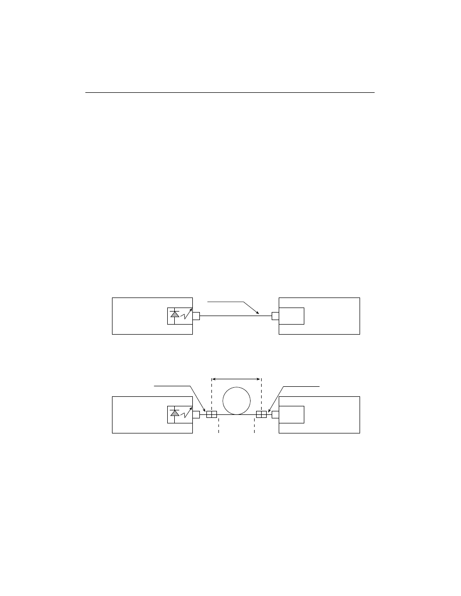
Figure 17-17

OFSTP-14 cable plant loss test as required in network

specifications.

connectors and then terminated in place, and connectors are the most likely prob-
lem to be uncovered by testing for loss. After installation and termination, each
segment of the cable plant should be tested individually as it is installed, to insure
each connector and cable is good. Finally, each end-to-end run (from equipment
placed on the cable plant to equipment) should be tested as a final check.

Testing the complete cable plant is done in accordance with another standard

test procedure, OFSTP-14 (Figure 17-17). This procedure covers the peculiarities
of multimode fiber in detail. In fact, it was written for multimode cables to cover
the problems of controlling mode power distribution, but the same procedures
apply for singlemode fiber, less the concerns expressed for mode power distribu-
tion errors.

For multimode fibers, testing is now usually done at both 850 and 1300 nm,

using LED sources. This will prove the performance of the cable for every data-
com system, including FDDI and ESCON, and meet the requirements of all net-
work vendors. For singlemode fiber cables, testing is usually done at 1300 nm,
but 1550 nm is sometimes required also. The 1550-nm testing will show that the
cable can support wavelength division multiplexing (WDM) at 1310 and 1550
nm for future service expansion. In addition, 1550-nm testing can show micro-
bending losses that will not be obvious at 1310 nm, since the fibers are much
more sensitive to bending losses at 1550 nm.

CHAPTER 17 — FIBER OPTIC TESTING

211

Light

Source

Optical Power
Measurement

Equipment

P

1

Test Jumper 1

Light

Source

Optical Power
Measurement

Equipment

P

2

Cable Plant

Test Jumper 1

Test Jumper 2

A

B

Reference Power Measurement for Method B

Cable Plant Loss Measurement

If cable plant end-to-end loss exceeds total allowable loss, the best solution is

to retest each segment of the cable plant separately, checking suspect cables each
way, since the most likely problem is a single bad connector or splice. If the cable
plant is long enough, an OTDR may be used to find the problem. Bad connectors
must then be repolished or replaced to get the loss within acceptable ranges.

What about OTDR Testing?

Once upon a time, OTDRs were used for all testing of installed cable plants. In
fact, printouts or pictures of the OTDR traces were kept on record for every fiber
in every cable. The power meter and source (or OLTS) have replaced the OTDR
for most final qualification testing, since the direct loss test gives a more reliable
test of the end-to-end loss than does an OTDR (see OTDR discussion above).

However, the OTDR may need to be used to find bad splices or ORL prob-

lems in connectors and splices in a singlemode cable plant. Only with an OTDR
can ORL problems be located for correction. Typical back reflection test sets
only give a total amount of backscatter or return loss, not the effects of individ-
ual components, which is necessary to locate and fix the problem.

The OTDR can also be used to find bad connectors or splices in a high loss

cable plant, if the OTDR has high enough resolution to see short, individual cable
assemblies. However, if the cables are too short or the splices too near the end of
the fiber (as is often the case in pigtails spliced onto singlemode fiber cables), the
only way to localize the problem is to use a visual fault locator, preferably a high-
powered HeNe laser type, which can shine through the jacket of typical yellow or
orange polyvinyl chloride- (PVC) jacketed single-fiber cables. This method of
fault location is easiest if single-fiber cables use yellow or orange jackets that are
more translucent to the laser light.

Handling and Cleaning Procedures

Connectors and cables should be handled with care. Do not bend cables too
tightly, especially near the connectors, as sharp bends can break the fibers. Do
not drop the connectors, as they can be damaged by a blow to the optical face.
Do not pull hard on the connectors themselves, as this may break the fiber in the
backshell of the connector or cause pistoning if the bond between the fiber and
the connector ferrule is broken.

COUPLERS AND SWITCHES

Some networks use passive couplers or switches to redirect the fiber path. These
devices must be tested for loss just as is any other component, although each pos-
sible light path needs testing individually. Multimode components will be sensitive
to mode power distribution and need to be tested carefully to get accurate results.

212

CHAPTER 17 — FIBER OPTIC TESTING

Fiber Optic Couplers

Couplers split or combine light in fibers. They may be simple splitters or 2

×

2

couplers, or up to 64

×

64 ports star couplers. Most are made by fusing fibers

under high temperatures, which causes light to split or combine in appropriate
ratios. Relevant specifications for couplers are the coupling ratios of each port or
the consistency across all the ports, crosstalk, and the excess loss caused by the
fusing. Excess loss is the difference between the sum of all the outputs and the
sum of all the inputs. When used in laser-based systems, couplers may need test-
ing for optical return loss and also for wavelength dependence.

Thus, testing couplers involves coupling a test source to each input port in

turn and measuring all the outputs for consistency, then summing all the output
powers and subtracting that number from the input power to calculate excess
loss. Connectorized couplers are tested like connectorized cables, using a launch
cable, whereas couplers with bare fibers must use a cutback method or a pigtail
and temporary splice to couple the launch source.

Singlemode couplers have another characteristic that must be considered:

They are very wavelength sensitive. Most couplers are optimized at one wave-
length unless they are specially designed for both 1310- and 1550-nm operation.
Some are even built to be wavelength division multiplexers, coupling light from
1310- and 1550-nm lasers into separate output ports. Therefore, sources for test-
ing couplers must be accurately characterized for wavelength to minimize mea-
surement uncertainty.

Fiber Optic Switches

Switches transfer light from one fiber to another. As with couplers, switch testing
involves measuring the loss in the switch by measuring the input from a source
and the appropriate output for each switch position. In multimode components,
mode power distribution can cause variation in switch losses or coupling ratios.

FIBER OPTIC DATALINKS

Fiber optic transmission systems all work similarly; they contain a transmitter
that takes an electrical input and converts it to an optical output from a laser
diode or LED. The light from the transmitter is coupled into the fiber with a
connector and is transmitted through the fiber optic cable plant. The light is ulti-
mately coupled to a receiver where a detector converts the light into an electrical
signal, which is then conditioned properly for use by the receiving equipment.
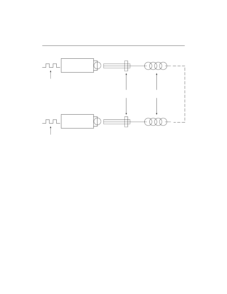
Most networks or datalinks will be bidirectional and full duplex, transmitting
and receiving simultaneously. They will have two links as shown in Figure 17-
18, operating in opposite directions. Just as with copper wire or radio transmis-
sion, the performance of the fiber optic data link can be determined by how well

CHAPTER 17 — FIBER OPTIC TESTING

213

the reconverted electrical signal out of the receiver matches the input to the
transmitter.

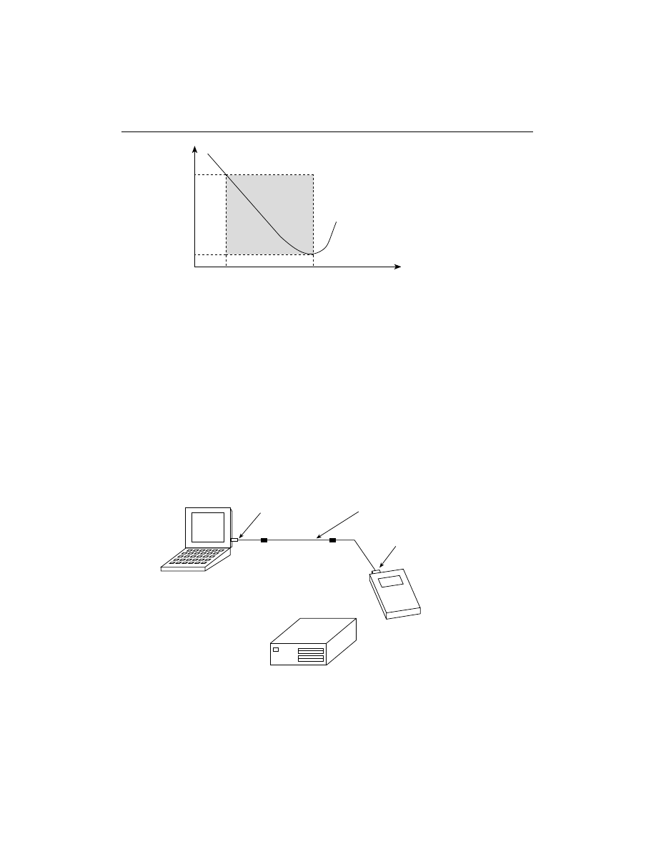
The ability of any fiber optic system to transmit data ultimately depends on

the optical power at the receiver as shown in Figure 17-19, which shows the
datalink bit-error rate as a function of optical power at the receiver. Either too lit-
tle or too much power will cause high bit-error rates. Too much power, and the
receiver amplifier saturates, too little and noise becomes a problem. This receiver
power depends on two basic factors: how much power is launched into the fiber
by the transmitter and how much is lost by attenuation in the optical fiber cable
that connects the transmitter and receiver.

Datalink testing is done with a power meter that measures the optical power

first at the receiver and then at the transmitter (with its power coupled into a
known good test cable, usually one of the launch cables used for testing the cable
plant) as shown in Figure 17-20.

What Goes Wrong on Fiber Optic Installations?

In installing and testing fiber optic networks, the first problem routinely encoun-
tered is incorrect fiber optic connections. A fiber optic link consists of two fibers,
transmitting in opposite directions, to provide full duplex communications. It is

214

CHAPTER 17 — FIBER OPTIC TESTING

Figure 17-18

Typical fiber optic link.

Transmitter

Source

Driver

Input

LED or Laser

Receiver

Output

Photodiode

Preamp/Trigger

Connectors

Cables

not uncommon for the transmit and receive fibers to be switched. A visual fiber
tracer will make it easy to verify the proper connections quickly. The visual tracer
can trace the fiber through the cables, patch panels, and other components to the
far end.

If the fibers are connected correctly but the network still does not work, the

next thing to check is the receiver power level. If the receiver power level is within
specification, the problem is likely in the network electronics. If the receiver
power is low, test the transmitter power to see if it is within specifications. If
transmitter power is adequate, the cable plant is the problem.

Test the complete cable plant—including all individual jumper or trunk

cables—for loss, using a power meter and source and the double-ended method

CHAPTER 17 — FIBER OPTIC TESTING

215

Figure 17-19

Bit-error rate (BER) performance of fiber optic systems.

BER

Received Optical Power

Operating

Range

Max

Min

Min

Max

Figure 17-20

Troubleshooting a fiber optic link.

Transmitter Power

Cable Plant Loss

Receiver Power

described in the section on testing the installed cable plant. Use the double-ended
method, since system margin specifications include the loss of connectors on both
ends of the fiber. If the end-to-end (transmitter to receiver) loss measurement for
a given fiber is within the network margin specification, the data should be
recorded for future reference.

If the loss is too low, notation should be made that that fiber will probably

need an inline attenuator to reduce receiver power to acceptable levels. If the loss
is too high, it will be necessary to retest each link of the complete cable run to
find the bad link.

Possible causes of high end-to-end link loss are bad connectors, bad splice

bushings in patch panels, cables bent too tightly around corners, broken fibers in
cables, or even bad launch or receive cables or instruments. There are only two
ways to find the problem: testing each segment of the cable individually to find
the problem and issuing an OTDR if the lengths are long enough for viewing
with the limited resolution of the OTDR.

Do not use an OTDR for measuring end-to-end loss. It will not accurately

measure actual link loss as seen by the actual transmitters and receivers of the
fiber optic link. As normally used, the OTDR will not count the end connectors’
loss. The OTDR uses a laser with very restricted mode power distribution, which
minimizes the loss of the fiber and the intermediate connectors. Finally, the dif-
ference in backscattering coefficients of various fibers leads to imprecise connec-
tor loss measurements.

Surviving with Fiber Optics

Once the installation is complete, the cable plant tested, the network equipment
running smoothly, what is likely to go wrong in a fiber optic network? Fortu-
nately, not much. One of the biggest selling points for fiber optics has been its
reliability. But there are potential problems that can be addressed by the end user.

With the cable plant, the biggest problem is what the telcos call “backhoe

fade,” where someone mistakenly cuts or breaks the cable. Although this most
often happens when an underground cable is dug up, it can happen when an elec-
trician is working on cables inside a building. Outdoors, the best defense is to
mark where cables are buried and bury a marker tape above the cable that will, it
is hoped, be dug up first. Inside buildings, using orange or yellow jacket cable
instead of black or gray will make the fiber cable more visible and distinctive.
Outside cable faults are best found by using an OTDR to localize the fault, then
having personnel scout the area looking for obvious damage. Inside buildings, the
short distances make OTDRs unusable, so a visual fault locator is necessary.
Another problem is breaking the cable just behind the connectors in patch panels.

216

CHAPTER 17 — FIBER OPTIC TESTING

This is a difficult fault to find, but a visual fault locator is often the best way.
Unless the jumper cables are quite long, an OTDR will not help at all.

Within the fiber optic link, the most likely component to fail is the LED or laser

transmitter, since it is the most highly stressed component in the link. Lasers are
feedback stabilized to maintain a constant output power, so they tend to fail all at
once. LEDs will drop in power output as they age, but the timeframe is quite long,
100,000 to 1 million hours. If there is no power at the receiver the next place to
check should be the transmitter LED or laser, just to isolate the problem to either the
transmitter or the cable plant. Receivers are low-stressed devices and highly reliable,
but the electronics behind them can fail. If there is receiver power but no communi-
cations, a loopback test to see if the receiver is working is the best test of its status.

REVIEW QUESTIONS

1. _____________ is the most important parameter and is required for

almost all fiber optic tests.

a. Attenuation

b. Backscatter

c. Optical power

d. Receiver power

2. Match the items on the left with related phrases on the right.

____ Power meter

a. detects a 2kH “tone”

____ OTDR

b. detects poor splices or cable breaks in

____ Fiber identifier

short lengths of fiber

____ Visible fault locator

c. measures optical power

____ Microscope

d. detects faults in long lengths of fiber

____ Attenuator

e. introduces a measured loss into the link
f. detects scratches and polishing defects

in connectors

3. Optical fiber is sometimes tested for _____________ before it is installed.

a. back reflection

b. splice loss

c. continuity

d. return loss

4. 0 dBm is equal to _____________

a. 1 mW.

b. –30 dBµ.

c. both a and b

d. neither a nor b

CHAPTER 17 — FIBER OPTIC TESTING

217

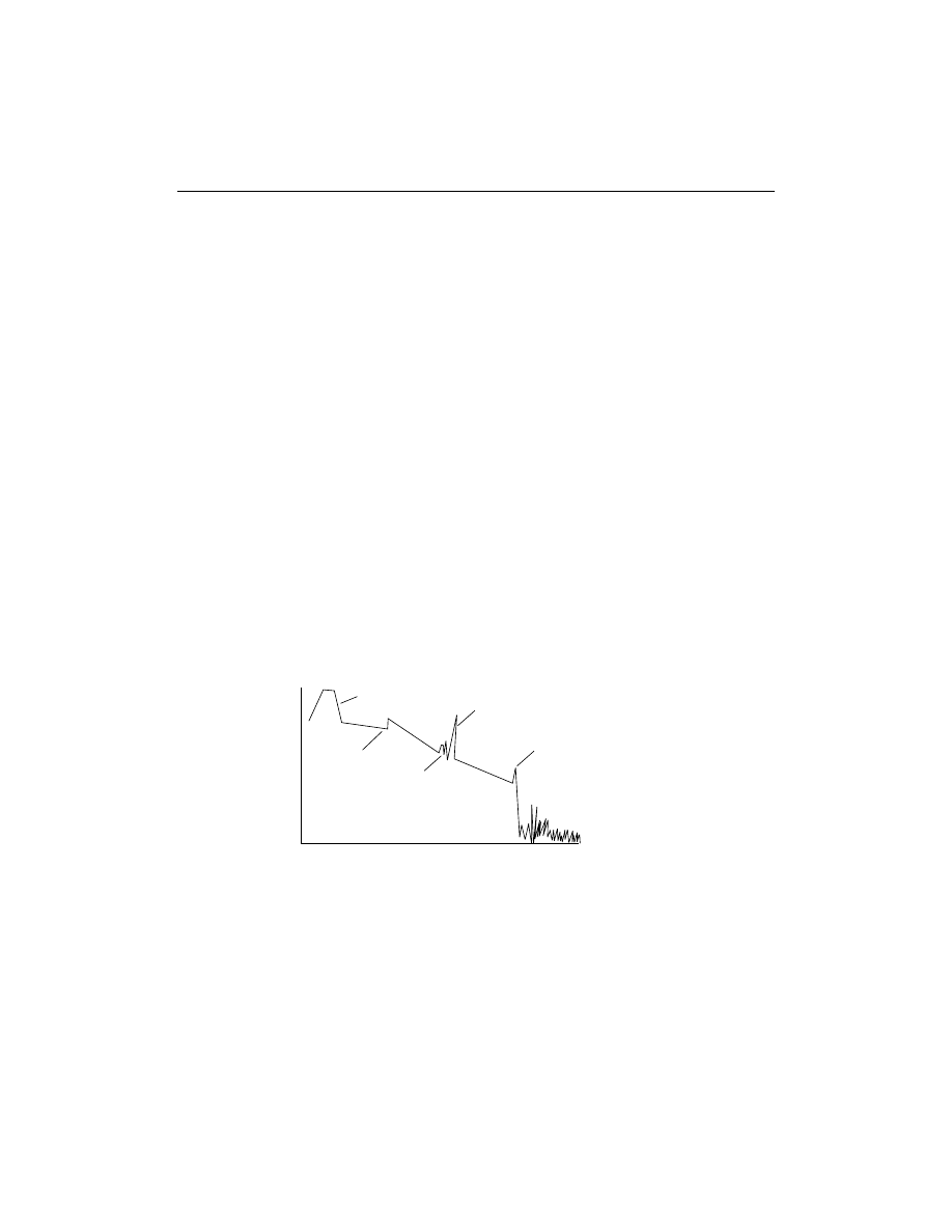
5. When testing for loss, the launch cable must be compatible with the

_____________

a. source wave length.

b. cable type.

c. fiber type (62.5, 50, SM).

d. length of the cable.

6. An OTDR uses _____________ to characterize fibers and find faults.

a. absorption

b. attenuation

c. backscattering

d. LEDs

7. One advantage an OTDR has over a power meter and source is

_____________

a. lower price.

b. more accurate attenuation reading.

c. it requires access to only one end of the fiber.

d. no measurement uncertainty.

8. To detect splice loss in a 1.5 km yellow-jacketed SM fiber a

_____________ is used.

a. OLTS

b. OTDR

c. Visual fault locator

d. OCWR

9. Using the accompanying trace, identify the following:

1. splice _______
2. initial pulse _______
3. connector _______
4. end of fiber _______
5. back reflections _______
6. gain _______

Distance

dB

E

A

D

B

C

218

CHAPTER 17 — FIBER OPTIC TESTING