Copyright 2009 Kenneth A. Johnson
Last updated May 25, 2009
KinTek Global Kinetic Explorer™
Version 2.0.13
with FitSpace Explorer
TM
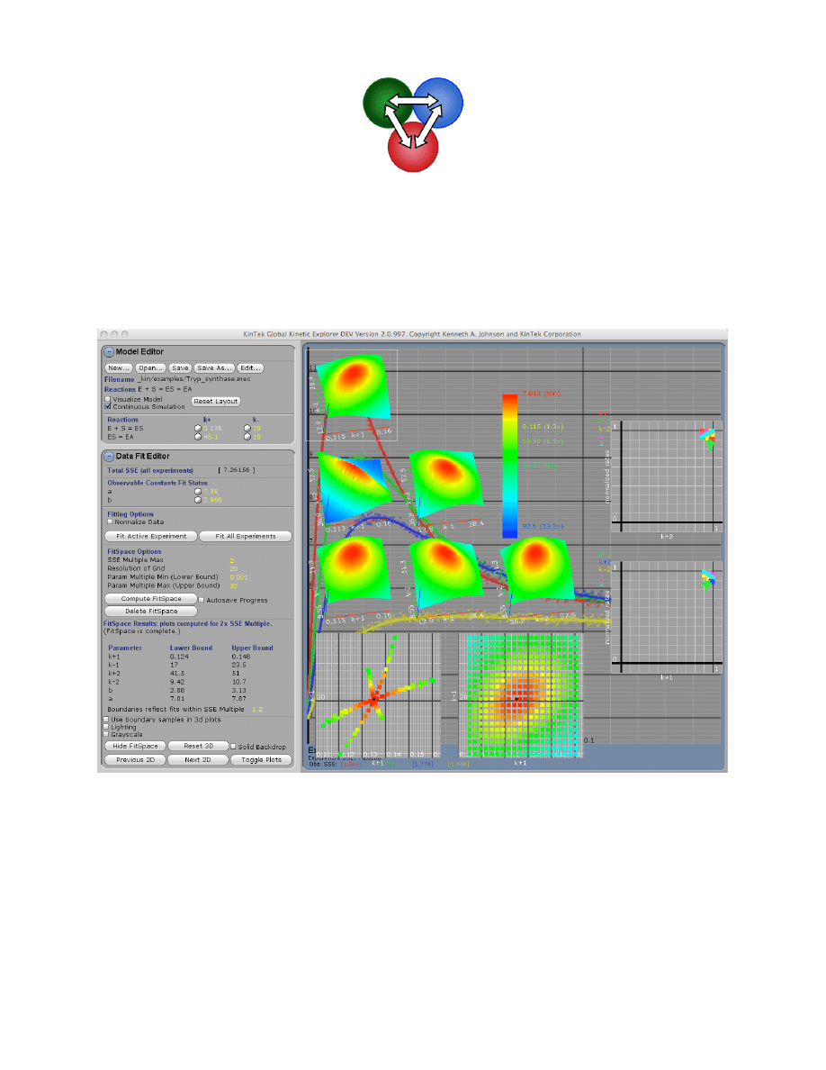
This figure shows the fitting of four stopped-flow experiments to define the kinetic constants for the reaction of
serine with pyridoxal phosphate at the active site of tryptophan synthase [1]. Superimposed on the fitted curves are
the 3D FitSpace confidence contours of the fitted parameters, showing that all parameters are well constrained by
the data.

ii
Published by KinTek Corporation, Austin, TX
Copyright 2009, Kenneth A. Johnson
Users of KinTek Global Kinetic Explorer
TM
(KinTek Explorer
TM
) are hereby granted
permission to reprint and distribute this instruction manual in its entirety for use in
teaching and research. Reproduction of individual figures or sections of the text is not
permitted without the written permission of the author. Permission can be requested at
kajohnson@kintek-corp.com.
System Requirements:
Windows XP or Vista with 1GB memory and a graphics card capable of running
open GL. In general any graphics card works. The only problems we have
encountered are when the system emulates open GL, and then the operation becomes
very sluggish. Please try the free Student software before ordering the Professional
version.
Mac OSX 10.4.11 or later. Two version are available, one for Intel based computers
and one for the earlier Power PC computers.
Warranty:
This software is offered without warranty. The user assumes all risk including
consequences resulting from the use of this software.

iii
Table of Contents
General Features and Installation of the Software.................................................................... 1
Installing the program ...................................................................................................................... 1
Running the program ....................................................................................................................... 2
Dynamic Simulation............................................................................................................ 2
Nonstandard Features ........................................................................................................ 2
Mouse Operations............................................................................................................... 3
Other Functions .................................................................................................................. 3
Standard Nomenclature.................................................................................................................... 4
New Features in Version 2.0 ........................................................................................................ 5
Overview ........................................................................................................................................ 7
Program Flow Chart......................................................................................................................... 8
Model Editor.................................................................................................................................. 9
Entering the model ........................................................................................................................... 9
Species names ................................................................................................................... 10
Saving and Editing the current model .............................................................................. 10
Display Control................................................................................................................. 11
Entering Rate Constants................................................................................................................. 11
Round-off Errors............................................................................................................... 12
Linked or Fixed Rate Constants........................................................................................ 12
Equilibrium Constants ...................................................................................................... 13
Modeling Steady State Kinetic Data ................................................................................. 13
Experiment Editor ...................................................................................................................... 14
Observable Output Expressions ..................................................................................................... 15
Examples of output expressions ........................................................................................ 15
Global Output Factors with Multiple Experiments .......................................................... 16
Concentration Series......................................................................................................... 16
Experiment Time ............................................................................................................... 17
Multiple Experiments..................................................................................................................... 17
Selecting the Active Experiment........................................................................................ 17
Controling the Simulation and Display ............................................................................ 17
Normalizing Data........................................................................................................................... 18
Scaling Factor Error Analysis .......................................................................................... 19
Data Normalization Example ........................................................................................... 20
Multiple-Mixing Experiments ....................................................................................................... 21
Importing Data ............................................................................................................................... 21
Importing a single reaction data file ................................................................................ 22
Importing data with a Concentration Series..................................................................... 23
Importing data with reactions of multiple species............................................................ 24
Generating Synthetic Data................................................................................................ 25
Exporting Simulation Results ........................................................................................................ 25
aFit Analytical Fitting Function..................................................................................................... 25
Plot Rate versus Concentration ........................................................................................ 26
Data Fit Editor ............................................................................................................................ 27
Controlling Rate Constants ............................................................................................................ 27
Fitting Experiments to the Model .................................................................................................. 28
Exporting Fit Results ........................................................................................................ 28
Plotting Confidence Intervals ........................................................................................... 29

iv
Error Analysis................................................................................................................... 29
Summary of Steps in Fitting Data.................................................................................................. 30
FitSpace Editor............................................................................................................................ 32
Confidence Contours ..................................................................................................................... 32
FitSpace Display ............................................................................................................................ 34
FitSpace Options ............................................................................................................................ 36
Errors on fitted parameters............................................................................................................. 38
FitSpace Boundary Error Limits ...................................................................................... 38
Plotting Confidence Intervals ........................................................................................... 39
Appendix...................................................................................................................................... 41
Example Files................................................................................................................................. 41
Tutorial Problem Set ...................................................................................................................... 46
Literature Cited .............................................................................................................................. 50
Troubleshooting ............................................................................................................................. 52
Downloading Updates.................................................................................................................... 52
Citing KinTek Explorer ................................................................................................................. 52

1
General Features and Installation of the Software
KinTek Global Kinetic Explorer
affords dynamic visualization and global fitting of multiple
data sets to a single unifying model. Using a fast and efficient algorithm, KinTek Explorer
simulates complex reaction schemes by numerical integration, built upon a simple and intuitive
user interface. A reaction scheme is entered using standard reaction sequence notation. The
starting concentrations of reactants then define each experiment and estimates of rate constants
form the basis for the simulation of each experiment. Each rate constant or starting concentration
can then be adjusted while the display is dynamically updated to show the effect of the change.
This powerful interface provides direct feedback to the user to develop understanding of
complex relationships between reaction mechanism, rate constants and observable reactions.
Moreover, visual estimation can be used to fit multiple data sets simultaneously, and evaluate the
results from nonlinear regression fitting algorithms. KinTek Explorer is ideal for students who
are first learning kinetics but is also a cutting edge tool for the most challenging data fitting
problems.
KinTek Explorer is offered in two versions. A free student version is ideal for teaching
and exploring kinetics but is limited in that only the defined example files provided with the
software can be opened. The Professional version allows files to be saved and data to be
imported and fitted. By purchasing the Professional license, you are supporting our ongoing
efforts to continue to expand the capabilities of the software.
Global fitting of a family of data sets to a single model should be approached with a good
deal of understanding and a healthy dose of skepticism. On the one hand, fitting to a family of
curves simultaneously is more robust in that it reduces the number of independent parameters
required to fit the data and maintains the relationships between rates and amplitudes of reactions
that are often lost in conventional data fitting. On the other hand, with the power of computer
simulation, it is too easy to include additional steps in a model that are not defined by the data.
KinTek Explorer is intended to help you recognized when a model is overly complex both by
statistical analysis of fitted parameters, but also by visual exploration of the multi-parameter
landscape. FitSpace Explorer provides reliable estimates of errors on fitted parameters and
reveals complex relationships between fitted parameters.
Installing the program
1. Download the appropriate version of the software (see list below) from the KinTek website:
http://kintek-corp.com/kinetic_explorer/
There are three versions of the Professional software available for different platforms:
For PC: KinTek_Explorer_Pro_win32.zip
For Mac Power PC: KinTek_Explorer_Pro_macosx_ppc.tar.gz
For newer Mac Intel processor: KinTek_Explorer_Pro_macosx_intel.tar.gz
and three versions of the Student version of the software:
For PC: KinTek_Explorer_Student_win32.zip
For Mac Power PC: KinTek_Explorer_Student_macosx_ppc.tar.gz
For newer Mac Intel processor: KinTek_Explorer_Student_macosx_intel.tar.gz
2. Uncompress the file and place the KinTek_Explorer_Pro folder anywhere on your hard drive.

2
You will find two subdirectories:
docs contains this instruction manual, plus a tutorial and a sample exam. Please take the
time to read through the instructions to learn the full power of the software. There are
several unusual features of the software that are not likely to be discovered by trial and error.
_kin contains the examples folder with 40 example files and the rawData folder showing
several examples of data file formats for importing your data.
USB key:
To run the Professional version, the USB hardware key that came with the program
must be inserted into a USB port for the program to run. The program can be installed on
multiple computers, including a mixture of Mac and PC computer, but can only be run on one
computer at a time.
Be careful to not loose the USB key. Replacement cost is equal to the cost of the original license.
Student Version:
The Student/Demo version of the program does not require the USB hardware
key. However the Student/Demo version is limited in that you cannot save files, import data, or
open any files other than the set of mechanism files in the examples directory. Other than that,
the program retains the full functionality of the Professional version.
Running the program
Double click on the KinTek_Explorer.exe (or KinTek_Explorer.app) file to run the program. The
program will open with a simple mechanism. You can see other examples by clicking Open and
selecting from the list. To immediately see the power of this program, click on any rate constant,
concentration, or scaling factor with the mouse, and while holding the mouse button down, drag
the value up or down and see the effect on the shape of the curves.
Dynamic Simulation
Dynamic Simulation provides a powerful tool that can help you decide which rate constants are
the most important. Careful analysis by trial and error will soon reveal which constants are
constrained by the data and which are not, both before and after fitting. Moreover, it can readily
reveal when your model is overly complex in that it includes steps that are not defined by the
data. You can control this function using the Continuous Simulation check box; if the box is
checked, the simulation is updated as you drag any rate or concentration up/down with the
mouse; alternatively, if the Continuous Simulation is not checked, the simulation is performed as
soon as you let go of the mouse button. The latter function is useful when you are initially setting
up a simulation or if the model is very complex.
Nonstandard Features
There are three non-standard features in the current version of the program. (1) The left hand
panel can be scrolled up and down by right-clicking on it and dragging the mouse up and down
or by rolling the middle mouse wheel. (2) Rate constants, concentrations and output factors can
be scrolled up or down by clicking on an entry and dragging the mouse up or down;
alternatively, if you click and release on an entry, you then can enter a value into the text box, as
described below. (3) Double-click is not enabled for any functions, most notably, in opening
files; rather click on the file name to highlight it, then click on “Open”.

3
Mouse Operations
The program takes full advantage of a three-button mouse. You can purchase a 3-button mouse
for a Mac computer or use Ctrl-click to get a right click function. On a Mac laptop, drag two
fingers on the touch pad to get the scroll function.
Left click to change parameters: There are two operations. If you click and release on a
parameter, a cursor will appear in a text box and you can then edit the number or enter a new
number. Entry is terminated by the Enter key on your keyboard or by clicking anywhere
outside of the text box. If you click and hold the mouse button down, you can drag the value
up and down with the mouse. Note that rates and starting concentrations can be changed
either on the Display Model or in the control panel.
Left click to arrange the display model: Left click on species in the display model and drag
with the mouse to a new location. It helps to uncheck Display Model Values, so that you will
not inadvertently change a rate or concentration while trying to relocate elements of the
model.
Right click to move the model: Right click anywhere on the Display Model and drag the
mouse to move the model to a new location.
Right click on the control panel: The control panel is one continuous list of items that
expands as the model increases in complexity or to display fitting options and results. Right
click anywhere on the control panel and drag the panel up or down with the mouse.
Middle mouse wheel: Roll the middle mouse wheel to scroll the control panel up/down or to
scan up/down in the file open and file save menus.
Middle button: Click and drag or use the rotary mouse button to alter the scale on the graph.
You can also use the Autoscale Plot button in the control panel to turn on and off the auto-
scaling function. The middle button also allows you to view the ~ 3D plots of confidence
contours from various angles; simply click on a contour and drag the mouse.
Other Functions
There are some useful functions accessed by using the Control key (Ctrl)
Ctrl-R Reload the last saved version of the current mechanism file
Ctrl-D Hide the Control Panel so the graph can be shown full screen; this is useful when
using a video projector.
ESC Hit the escape button to exit from a scrolling operation or text entry and reset the value
of the parameter to it starting value.

4
Standard Nomenclature
In reference to rate constants in this manual, we will use the standard numbering scheme as
illustrated below. Rate constants are numbered sequentially with a positive number for the
forward rate constant and a negative number for the reverse rate constant, in the direction written
when the model was defined.
In using the program, no reference to numbered rate constants is needed because the user
interface relates rate constants directly to individual steps; however, in discussing the variables in
this manual, we need to refer to numbered constants.
Citing KinTek Explorer
Two papers describing the use of the KinTek Explorer and FitSpace Explorer are in press in
Analytical Biochemistry [2; 3]. Please reference these papers in citing the use of KinTek
Explorer.
Johnson, K. A., Simpson, Z. B., and Blom, T. (2009) Global Kinetic Explorer: A new computer
program for dynamic simulation and fitting of kinetic data. Analytical Biochemistry 387, 20-29.
Available online: http://dx.doi.org/10.1016/j.ab.2008.12.024
Johnson, K. A., Simpson, Z. B., and Blom, T. (2009) FitSpace Explorer: An algorithm to
evaluate multi-dimensional parameter space in fitting kinetic data. Analytical Biochemistry
387,30-41. Available online: http://dx.doi.org/10.1016/j.ab.2008.12.025
E
+ S
k
1
k
−1
⎯ →
⎯⎯
← ⎯
⎯⎯
E
iS
k
2
k
−2
⎯ →
⎯⎯
← ⎯
⎯⎯
E
iX
k
3
k
−3
⎯ →
⎯⎯
← ⎯
⎯⎯
E
iP
k
4
k
4
⎯ →
⎯
← ⎯
⎯
E
+ P

5
New Features in Version 2.0
New features added to the program starting with Version 2.0 are listed in reverse chronological
order.
Font color/bold:
The font for the scrollable parameters can be toggled between yellow and green
using CTRL-H, and between bold and regular using CTRL-B.
Exclude Experiment from Global Fits:
This check box under the Experiment Editor allows you
to exclude a given experiment when fitting all experiments globally. This is useful when during
initial exploration to find a global fit and to explore the effect of a given data set on the global fit.
Note that the Fit Active Experiment function always allows you to fit a single experiment.
Normalize data within a concentration series:
Fitting data globally is often difficult because
minor fluctuations in lamp intensity in an instrument can lead to variations in signal for various
experiments within a given concentration series. We now enable an option to normalize the data
when fitting by computing a scaling factor to correct for variations in signal intensity. For this
approach to be valid, do not subtract a baseline from your data other than a background value
obtained by direct measurement. See instructions below for more information.
Integrator Error Tolerance:
(default value 2e-8). This value controls the error tolerance during
numerical integration. Use the default value unless your system produces less than 20 simulation
points. Set it to a smaller value to get more closely spaced simulation points.
Log10 Timescale:
Data and simulations can now be graphed on a log(10) timescale, which is
useful when examining processes that occur over a wider range of times.
Display of all possible fitted curves:
A new function allows you to overlay on the data and the
best fit a series of curves calculated from all parameters limits, based either upon the standard
error or the Fitspace boundary limits. This display allows you to evaluate the relationships
between the error limits on parameters and the data.
Video Projection Mode
:
When working with a small portable computer or during video
projection, the screen resolution is limited and that may make the graph too small relative to the
control panel. You can toggle the control panel on/off by pressing Ctrl-D to see the graph on the
full screen. If you start to scroll a value before pressing Ctrl-D, you can continue scrolling. You
can also use the Display Model to scroll rate constants while the Control Panel is hidden.
Double Precision:
All calculations are now done in double precision (64-bit). You will note that
estimates of standard error have increased in those cases where the parameters are not well
constrained by the data. This can be understood as due to greater precision of the computation in
dealing with the ratios of very large numbers in calculating standard error for an under-
constrained system.
Faster Execution:
Improvements in the integrator make fitting and scrolling more than 10-fold
faster! Also, the user no longer enters the number of points to simulate; rather, the integrator
optimizes the step-size during simulation, and we do a spline interpolation to get additional
points to produce a smooth curve.
Dimer formation:
Version 1 did not properly handle mass balance of reactions involving
dimerization. The version 2.0 release resolved these issues.

6
Rate vs Concentration Plot:
You can fit your data or your simulation output to analytical
functions by nonlinear regression using the aFit function. If you have a series of traces collected
at several concentrations, you can click on Rate v Conc and see a graph of the concentration
dependence of the observed rates. This is useful in revealing patterns in the data that suggest the
underlying mechanism [4].
No more Reverse Polish Notation:
Entry of output expressions now uses the more familiar infix
notation. The first time you load an old mechanism file created under Version 1, you will be
required to convert your output expressions to infix notation. This is explained in more detail
under Experiment Editor.
FitSpace Explorer:
Given the power and ease of use of KinTek Explorer, it is too easy to enter
an overly complex model and often difficult to evaluate whether the model and the rate constants
are actually determined by the data. Conventional error analysis fails to notify you of the full
extent of variability when parameters are under-constrained. Therefore, it is difficult to evaluate
the extent to which the fit and the model are constrained by the data especially when fitting
multiple parameters to multiple data sets simultaneously. FitSpace Explorer solves these
problems by exploring the range over which parameters can vary and still achieve a good fit to
the data. This analysis provides more realistic estimates of errors on fitted parameters than are
obtained by conventional nonlinear regression covariance analysis.
7
Overview
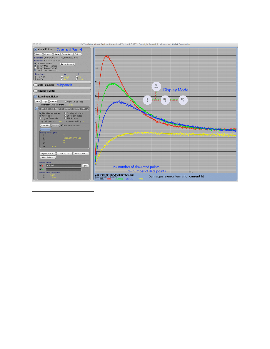
Example: Tryp_synthase.mec. This figure shows the division of the window into the Control
Panel (left) with its four subpanels and the graphic panel (right). The Control Panel can be
scrolled up and down to access individual functions and each subpanel can be expanded or
contracted by clicking on the + or – next to the name (i.e., Model Editor). The Display Model
shows the current mechanism, rate constants and starting concentrations. Beneath the graph, the
numbers display the high and low values for the number of simulated points (n) and number of
data points (d) across the concentration series. In addition, the total sum square error and
individual sum square error values for each trace are shown.
Control functions will be described for each group in the order in which they are used:
Model Editor:
Enter model and estimates for rate constants
Experiment Editor:
Set up each experiment and import data.
Data Fit Editor:
Fit data and enter values for scaling factors
FitSpace Editor:
Examine the space over which parameters can vary
Note that the subpanels are grouped in the Control Panel in an order that optimizes their use.
For example, data are fit only after defining the model, the experimental conditions and
importing data, but the Data Fit Editor is placed just beneath the Model Editor so that controls
over rate constants will be conveniently located when fitting data.
8
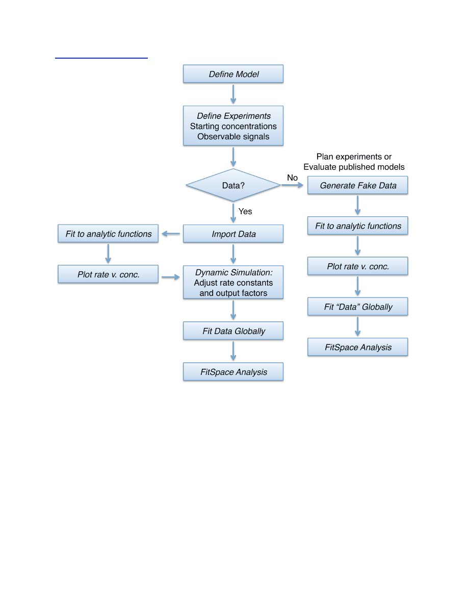
Program Flow Chart
9
Model Editor
Under Model Editor you will:
• Define a model
• Enter rate constants
•
Constrain rate constants
Entering the model
The Model Editor contains functions to open and save mechanism files, to create new models,
and to enter and control rate constants.
Click to open an existing mechanism. Use a single click to navigate to the directory
containing mechanism files and the select the desired file. You can also use the middle mouse
wheel (or right-click and drag) to scroll up and down the listings. Then click OK to open the file.
You can restrict the directory search by entry in the command line at the bottom of the screen.
By default, the entry is /*.mec. Changing the entry to /T*.mec, for example, will cause the
display of only the mechanism files that begin with the letter T. The entry is case sensitive.
NOTE: Our user interface does not support the common “double-click” function.
Click to create an entirely new model, then enter the reaction sequence with an = sign to
designate a reaction as illustrated in this example:
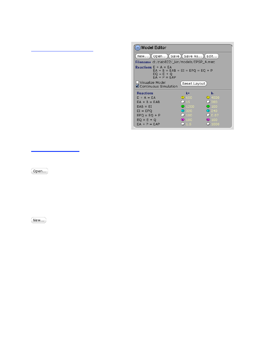
E + S = ES = EI = EP = E + P
Note that as you type, the program will continuously parse the model and warn you of syntax
errors.
The reaction can continue on one line as long as mass balance is maintained. More complex
pathways such as EPSP synthase require multiple lines to maintain mass balance:
E + A = EA
EA + B = EAB = EI = EPQ = EQ + P
EQ = E + Q
Note the error in the following (unless you intended to mean that B was produced when A
reacted with E):
E + A = EA + B = EAB

10
Species names
The names given for reactants are case sensitive and may contain any unique set of alphanumeric
characters plus the following special characters, but no others.
~ . $ #
These characters can be used to help distinguish complex terms such as E.D.dNTP or
E.NADPH.DHF, or E.Tyr~AMP.PP. However, you should keep the names as short as possible
while using terms that you recognize easily. The EPSP synthase pathway could have been
written:
E + S3P = E.S3P
E.S3P + PEP = E.S3P.PEP = EI = E.EPSP.P = E.EPSP + P
E.EPSP = E + EPSP
Note that because the species names are case sensitive, ES and Es would be considered as
different species.
Reactions involving the simultaneous collision of three species are not allowed. For example it
may be common to write the following enzyme-catalyzed reaction when the order of product
release is not known:
E + S = ES = EPQ = E + P + Q
However, that implies the reverse reaction involving the simultaneous collision of P and Q with
the enzyme, which is a highly unlikely event. We enforce reasonable reactions at all steps and
preclude the entry of such a model. This reaction sequence can be entered instead as:
E + S = ES = EPQ = EP + Q
EP = E + P
If the order of product release is not known, simply make the rate constant for release of P faster
than that for release of Q, so that kinetically both steps occur at a single rate.
For completeness, a random order of product release steps can be specified by adding two
more lines:
EPQ = EQ + P
EQ = E + Q
Saving and Editing the current model
Save the current mechanism file (*.mec). Use a single mouse click to navigate to the
desired directory; you can also use the middle mouse wheel (or right-click and drag) to scroll up
and down the listings. Then type in the desired file name in the text box and the bottom of the
window, as illustrated by this example:
d:/KinTekExplorer/_kin/models/myenzyme.mec
NOTE: if data have been imported into the mechanism as described below, they will saved with
the mechanism file.
Save the current mechanism file under a new name.
Click to edit an existing reaction. This will open the text editor showing the existing
model. After editing the model, click Create to save changes, or Cancel to abandon changes.

11
NOTE:
If rate constants have already been entered, the program will attempt to match up
previous rates with the new model. If you change species that are already used as part of a
defined observable expression, the output will be flagged as an error with (
Orange Text
) under
Observables in the Experiment Editor. The output must be edited to continue. See additional
information below on the definition of output functions. If you intend to delete a species that is
part of a defined Observable output, it is safer to first remove that species from the output
expression before deleting it from the model.
Display Control
Click to center the Model and place species into the simplest geometric form. With
complex models, the species will need to be rearranged manually. This function also centers the
model in the graph window.
Visualize Model:
This checkbox controls whether the reaction model is displayed.
Display Model Values:
Turn off the values of rates and concentrations on the Display
Model while readjusting the positions of the species.
Display Large Format:
Toggle between large and small Model Display
Note that the Model Display can be useful for simple models, but can easily become difficult to
interpret for complex models. In these instances, it is better to turn off the Model display.
Continuous Simulation:
When “Continuous Simulation” is checked, the output of the
simulation is continuously updated at you scroll a rate constant, concentration or output factor.
You may want to turn this function off when defining a new experiment or fitting data.
Entering Rate Constants
Enter rate constants by putting the cursor over the red/green arrows connecting species, or on the
table in the control panel under the Model Editor. Click and drag to scroll values for rate
constants up/down, or click and release to enter a new rate.
Units
The program does not keep track of units, so you must be consistent. All rate constants need to
be in the same units of time as the data you may be fitting, i.e., s
-1
or m
-1
. Second order rate
constants must be in the same units of concentration as the concentrations of species used in the
mechanism. We recommend use of time in seconds and concentrations in micromolar, so all
second order rate constants are in units of µM
-1
s
-1
. Most second order rate constants are between
0.01 and 100 µM
-1
s
-1
, although an upper limit for diffusion may be as high as 1000 µM
-1
s
-1
. First
order rate constants relevant to enzyme catalysis are typically in the range of 0.001 to 10,000 s
-1
,
but can exceed this range.
Use of rate constants larger than 10,000 s
-1
often means that the model is overly complex
and the fast step contributes nothing to the observable kinetics (unless you have data collected on
the microsecond time scale). In some cases it may be that you only can model a step as a rapid
equilibrium or only place a lower limit on a given rate constant. In other circumstances the
model may need to be simplified.
12
Round-off Errors
It is best to keep time, rate constants and concentrations between the values of 1x 10
6
and 1x10
-6
to avoid round-off errors that can affect fitting when using very large or very small numbers.
Linked or Fixed Rate Constants
Often in fitting, you want to maintain the ratio of two or more rate constants at a fixed value and
then change the rates in unison while maintaining that constant ratio. This is particularly
important to maintain the equilibrium constant off while searching for an optimal or minimal
rate. The tool is useful before, during and after fitting. Control is achieved using the following
set of symbols adjacent to the rates on the table under Model Editor:
Click on the control to sequentially step through the 11 options. Right-click clears the selection.
Rates can be grouped into one of 9 sets by selecting one of the number symbols listed above. At
the time the rate is added to a group, all rates in that group become linked by a constant ratio
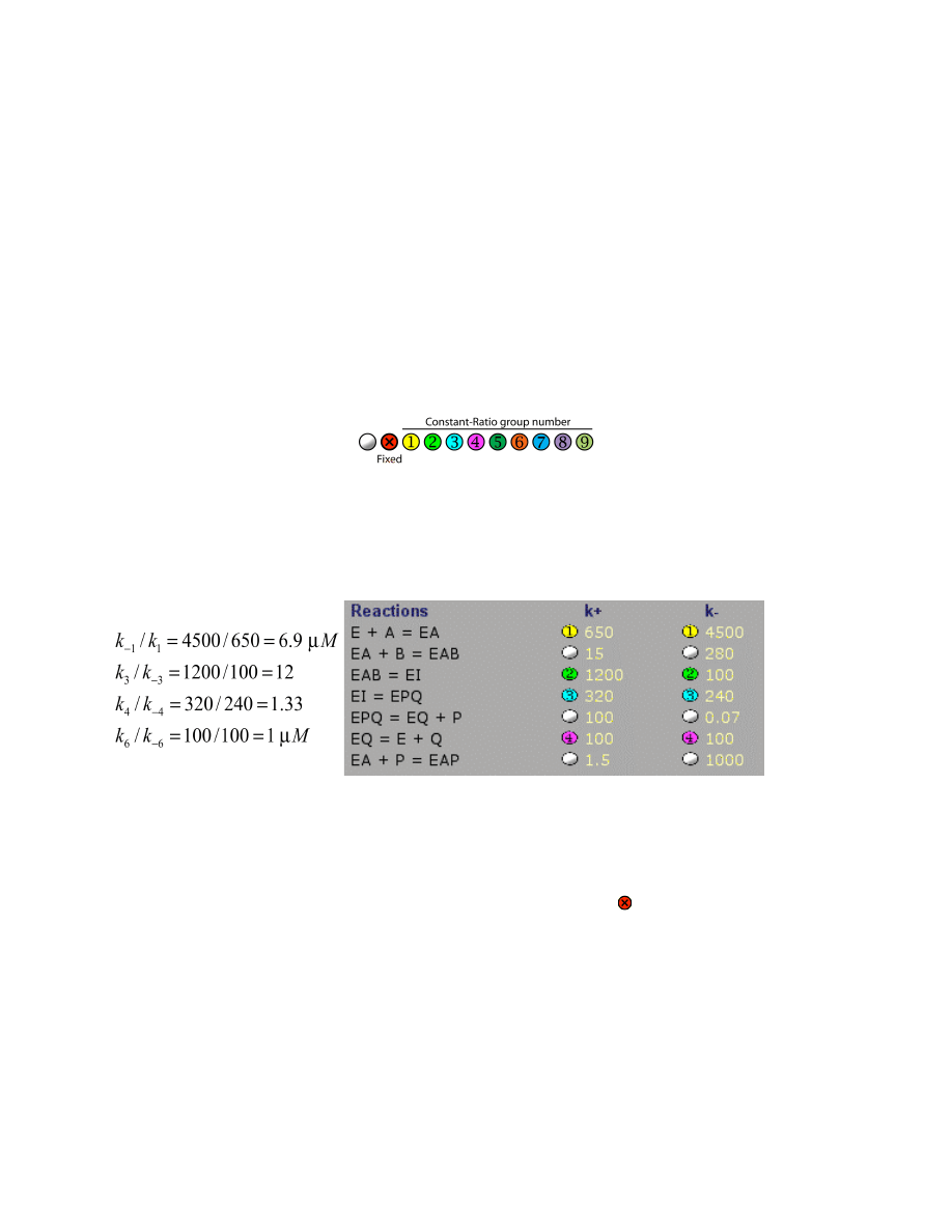
defined by their values when they are added to the group. For example, for EPSP synthase there
are four grouped rates:
These constant ratios provide important constraints in fitting the data by including information to
define the equilibrium constants for these 4 steps of the reaction.
NOTE:
The constant ratio applies both when scrolling the rate constants and in fitting the data by
nonlinear regression.
In order to hold a given rate constant fixed during fitting, select the symbol next to the rate
constant. The rate constant can still be scrolled or changed by text editing, but it will be held
fixed at the value when fitting by nonlinear regression.
13
Equilibrium Constants
We do not support the explicit fitting of an equilibrium constant because such fitting requires
that the reactions be infinitely fast, and that is never the case. Often a step in a sequence is
thought to be fast enough relative to other rates that it is essentially at equilibrium and there is no
information to define the rates. Under these circumstances, simply make the rates faster than
neighbors in the reaction sequence. Use of the linked rate constants and dynamic simulation is
useful to explore how fast the rates need to be to evaluate the fitting of the data to the model.
There are two options when fitting data, as illustrated below by fitting a binding constant:
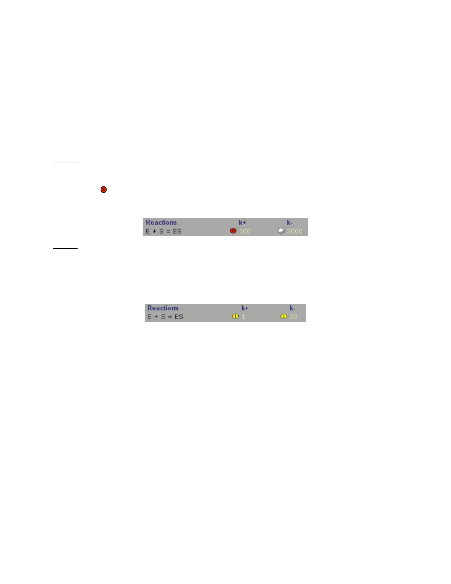
Case 1. You do not know the equilibrium constant, but believe it is rapid. In this example, set the
binding rate at the diffusion limit (nominally 100 µM
-1
s
-1
), and let the dissociation rate float
during fitting to determine the K
d
= k
-1
/k
1
. This is accomplished as shown below, using the fixed
rate function to freeze the binding rate, k
1
, in this model where K
d
= 20 µM. This analysis will
return the error estimates for k
-1
. The percentage error on the K
d
is equal to the percentage error
on k
-1
.
Case 2. You think you know the K
d
, but want to fit to see how fast the binding and dissociation
rates must be to account for the data. In this example, group the binding and dissociation rates so
that they are constrained to give the K
d
, and then fit the data allowing both rates to float in unison
(in this case k
-1
/k
1
= 20 µM). In the example shown below, k
1
and k
-1
belong to group 1 to
maintain the constant ratio. FitSpace explorer can then be used to determine the lower limit on
the values of k
1
and k
-1
.
Modeling Steady State Kinetic Data
In fitting steady state kinetic data there is not enough information to define all of the rate
constants in a minimal pathway. One can only define k
cat
and K
m
from the data.
E
+ S
k
1
k
−1
⎯ →
⎯⎯
←
⎯
⎯⎯
ES
k
2
k
−2
⎯
→
⎯⎯
←
⎯
⎯⎯
EP
k
3
k
−3
⎯
→
⎯⎯
←
⎯
⎯⎯
E
+ P
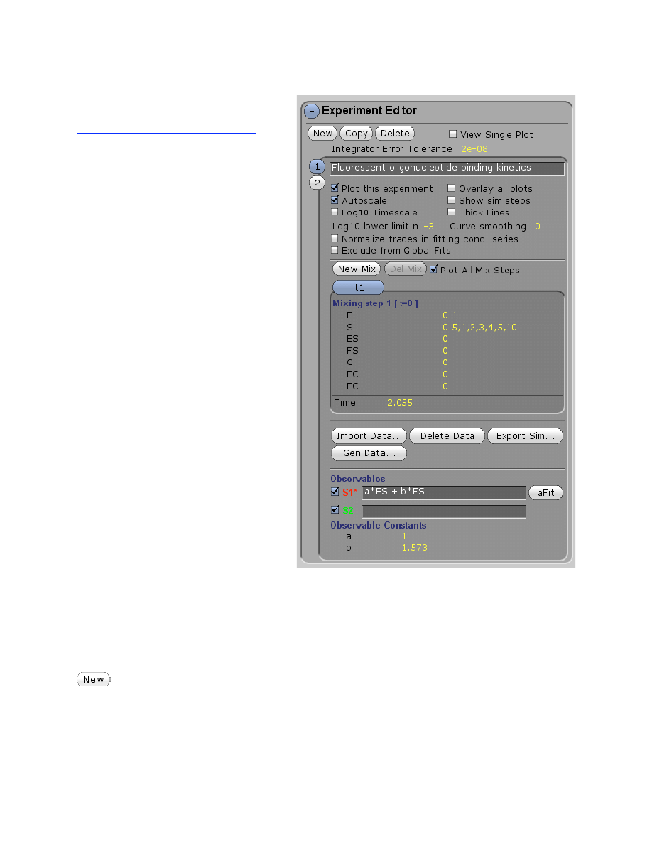
One simple approach is to fit to a rapid equilibrium model with substrate binding rates fixed at
the diffusion limit and then compute k
cat
and K
m
. The fitting does NOT imply one knows that
chemistry is rate-limiting in the steady state; rather, this simplification only allows computation
of k
cat
and K
m
by fitting to a simplified model. As additional experiments are added to the global
fitting, refined estimates for intrinsic rate constants can be used.
E
+ S
(1000
µM
−1
s
−1
)
k
−1
⎯
→
⎯⎯⎯⎯⎯⎯⎯
←
⎯
⎯⎯⎯⎯⎯⎯⎯
ES
k
2
k
−2
⎯
→
⎯⎯
←
⎯
⎯⎯
EP
k
3
(1000
µM
−1
s
−1
)
⎯
→
⎯⎯⎯⎯⎯⎯⎯
←
⎯
⎯⎯⎯⎯⎯⎯⎯
E
+ P
Forward reaction
k
cat
= k
2
K
m
= k
-1
/1000
Reverse reaction
k
cat
= k
-2
K
m
= k
3
/1000
14
Experiment Editor
Under Experiment Editor you will:
• Define new experiments
o Starting concentrations
o Reaction times
o Mulitple mixing events
• Define output observables
• Control graphical display
• Import data
• Generate fake data
• Export simulation results
• Fit to analytical functions (aFit)
• Control normalization of data
within a concentration series
In the Experiment Editor, you will define an experiment by specifying the starting concentrations
of reactants, the time interval of the reaction, and you will define the output you expect to be able
to observe. The Observable outputs are defined as sums of individual species, weighted by
output factors (such as extinction coefficients). In addition, the Experiment Editor controls the
importing of data. Several experiments can be defined within a given mechanism file and
globally fit to a single model.
To define the starting conditions for an experiment, in the Experiment Editor, control
panel click New and enter the starting concentrations, reaction time, and define the outputs. In
this example, there are four experiments, designated by the numbers 1-4 on the left hand edge.
Clicking on each number allows that experiment to be selected so that parameters
(concentrations, time, etc) that govern that experiment can be entered.

15
Observable Output Expressions
Outputs are defined to mimic the conditions under which data were collected to get an
observable signal. For example, in rapid quench experiments, the observable may be the sum of
all species with a radio-label, whether bound to the enzyme or free in solution. In absorbance
measurements, the signal may be the sum of all absorbing species weighted by their extinction
coefficients. Similarly, in fluorescence experiments, the signal may be a weighted sum of various
species. Remember that simulations are performed in units of absolute concentrations of species,
while all signals are a function of those concentrations, defined by the output factors or
extinction coefficients.
Examples of output expressions
Fluorescence:
Signal = a*E + b*ES + c*EP
Burst of product formation:
Signal = EP + P
Absorbance of S and P:
Signal = a*(S + ES) + b*(P + EP)
In the example in the Experiment Editor panel shown above, there are three output expressions
from this rapid quench experiment:
S1
: Q + EQ + EPQ represents the sum of all species containing the reactant Q
S2
: EI represents the enzyme-bound intermediate
S3:
EAB + B represents the sum of species containing the reactant B
The table below shows an example from burst.mec, with three outputs. Output S1 shows the
transient rise and fall of the species EA. Output S2 is a typical burst involving the sum of product
bound to the enzyme and free in solution. Output S3 is a hypothetical fluorescence change with
different extinction coefficients for each species.
Signal
Infix notation
S1
[EA]
S2
[EP] + [P]
S3
a*[E] + b*[EA] + c*[EP]
New outputs can be entered into the blank space for S4. An output can be deleted by deleting its
definition. In defining the output, anything that is not recognized as a species name is assumed to
be an output factor and a new item will appear to allow entry of values for the output factor.
The check box (
) allows the display of each output to be toggled on and off.
All output factors are constrained to be positive numbers
. This constraint is necessary to prevent
the automatic data fitting routines from wandering into nonsensical space (i.e., negative
extinction coefficients). If you need a negative number, subtract a positive number in your output
expression. However, in most instances the use of a negative output factor is probably not valid
because nearly all signals are the result of a weighted sum of concentrations of species.
E
+ S
k
1
k
−1
⎯ →
⎯⎯
← ⎯
⎯⎯
E
iS
k
2
k
−2
⎯ →
⎯⎯
← ⎯
⎯⎯
E
iP
k
3
k
−3
⎯ →
⎯⎯
← ⎯
⎯⎯
E
+ P

16
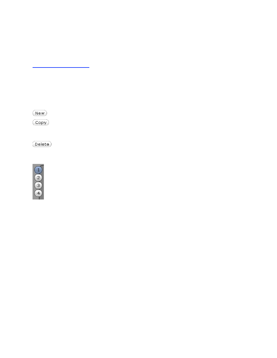
For example, a fluorescence change upon substrate binding can be modeled as:
The general output factor would then be given by the sum of the concentrations of each species
weighted by their fluorescence factor (a, b, c) plus a constant background (bkg):
a*E + b*ES + c*FS + bkg
Alternatively, if the fluorescence states of E and ES are thought to be identical, the output can be
simplified to:
a*(E + ES) + b*FS + bkg
If a < b, the signal will decrease with time as the reaction progresses. See Tryp_synthase.mec
and Burst_with_fluorescence.mec as examples, and note who the curves change in shape as the
relative magnitudes of the output factors change.
It is often useful to write an expression in a form such that the output factors give a fractional
fluorescence change relative to E, such as:
scale*(E + a*ES + b*FS) + bkg
You can use any alphanumeric characters to represent output factors
so long as names are
distinct from the names of species. Any name that is not recognized as a species gets assigned as
an output factor. Look for errors in defining output expressions by scanning the list of output
factors. For example, if you mistakenly typed: f1*(E + ES) + f2*EFS + c, there would be four
output factors: f1, f2, c and EFS because EFS is not a species, so the program assumes it must be
an output factor.
Each output can be toggled on/off with the check box.
If there are data associated with a given
output, it will be included in global fitting. However, if a given output is not displayed
(unchecked box), then the data will not be included in global fitting.
Global Output Factors with Multiple Experiments
When you program the Observable outputs for multiple experiments, if you use a give output
factor term for more than one experiment, that factor will be identical for each experiment.
Alternatively, you must use different terms to describe output factors. For example in fitting two
fluorescence experiments, we may define the following two output expressions for two
experiments:
Experiment 1: scale1*(E + a*ES + b*FS) + bkg2
Experiment 2: scale2*(E + a*ES + b*FS) + bkg2
In this case, both experiments will be fit assuming the same percentage change in forming ES
and FS, but the different scaling and background factors will allow for variations in setup in each
experiment.
Concentration Series
One of the species can have multiple concentrations separated by commas to perform
simulations over a concentration series. In multiple-mixing experiments, a concentration series
can be employed only in one of the time periods.
E
+ S
k
1
k
−1
⎯ →
⎯⎯
← ⎯
⎯⎯
E
iS
k
2
k
−2
⎯ →
⎯⎯
← ⎯
⎯⎯
F
iS
17
Experiment Time
The experiment time (net time for the simulation) can be adjusted by entering a time or dragging
the time up/down with the mouse. The display will automatically rescale to the new time only if
the Autoscale Plot option is checked.
Multiple Experiments
You can click New or Copy to generate additional panels for more experiments. Each experiment
is defined by the individual starting concentrations. The rate constants entered on the mechanism
will be applied to all experiments. See EPSP_4.mec as an example. Numbered circles on the left
of the panel are used to select the currently active experiment. Entries for concentrations and
output factors affect only the selected experiment, while changes in rate constants apply to all
experiments.
Creates a new experiment without entries for starting concentrations or outputs
Copies an existing experiment. This is useful if several experiments are similar; after
copying an experiment, you can then edit the parameters that differ without having to define all
parameters of the new experiment.
Deletes the currently selected experiment.
Selecting the Active Experiment
Click on a number to select a given experiment. Note that the currently active
experiment is highlighted by a light blue colored border in the graphics panel. All
entries under the Experiment Editor apply only to the selected experiment. Data
fitting can be based upon either the Active Experiment or to All Experiments as
described under the Data Fit Editor.
Controling the Simulation and Display
Integrator Error Tolerance:
(default value 2e-8). This value controls the error tolerance during
numerical integration. In general, the default value should be used and it is not recommended
that the error tolerance be changed unless you see a problem of too few are too many points.
Optimal performance is obtained with 30-150 simulation points. Click on Show Sim Steps to see
the distribution of points. With fewer points, the curves show noticeable straight line segments.
With more points, the fitting takes more time. In general, the default value (2e-8) gives optimal
performance. Set the error tolerance to a smaller value to get more closely spaced simulation
points. For example, if your mechanism produces fewer than 20 points, you can improve the
quality by decreasing the integrator error tolerance; try 1e-10, for example. The minimum value
is 1e-12.
View Single Plot:
When multiple experiments are included, checking View Single Plot,
enables the display of only one plot at a time. This is particularly useful when working on a
laptop computer or when you need to closely inspect one of the experiments. You select the
Active Experiment by clicking on the numbered circle on the left.
Plot this experiment:
This function allows you to turn on/off individual plots when multiple
experiments are present. The state of the check box is saved for each experiment; therefore, if an
experiment is not displayed you will need to first select that experiment (see Selecting Active

18
Experiment, above) and then change the status of the Plot checkbox.
Autoscale:
This function allows you to turn on/off the auto-scaling of both x- and y-axes. By
default, the auto-scale is turned on. It is useful to turn this function off if you want to see the
trends in the output while changing a rate or concentration that affects the amplitude of the
reaction; otherwise, the continuous auto-scaling tends to obscure the effect.
Overlay other visible plots:
This function allows you overlay all visible experiments.
Show Sim Steps:
Turns on/off the display of the steps of the simulation as square black dots
on the simulated curve. Points obtained by spline interpolation are shown in white.
Thick Lines:
Toggles between thin and thick lines display of the simulation output. The
thinner dark line helps to see the simulation line when there are a lot of data points.
Log10 Timescale:
Turns on/off the display of data and simulations on a log time scale.
Log10 Lower Limit (n):
Sets the power of ten lower limit of the logarithmic time scale.
Curve smoothing:
(range 0-10) This function controls the number of points to add during the
spline interpolation between simulation steps to get a more smooth appearance. This parameter
does not affect data fitting, only appearance. See “Show simulation steps”.
Exclude from Global Fits:
This allows the selected experiment to be excluded during global
fitting. This is useful when fitting multiple experiments in order to explore the effect of a given
experimental data set on the global fit.
Normalizing Data
Normalize traces in fitting conc. series:
This function introduces an additional scaling factor
to normalize traces within a concentration series. This is useful to correct for fluctuations in lamp
intensity in fluorescence traces, for example. Although this function controls data fitting, it
applies only to a single experiment when there is a concentration series. We illustrate the
procedure for normalization by the following example.
1. Open the file, Tryp_synthase_lamp_error.mec, which shows an exaggerated example with 5-
18% fluctuations in signal intensity as illustrated in Figure A on the next page. Note that a good
global fit cannot be obtained because of fluctuations in signal intensity for each trace.
2. Check Normalize traces in fitting conc. series under the Experiment Editor. A scaling factor
is then defined and applied to normalize the traces during fitting. These scaling factors can be
seen under Data Fit Editor.
Signal a = scale_1a*(original definition)
Signal b = scale_1b*(original definition)
Signal c = scale_1c*(original definition)
Signal d = scale_1d*(original definition)
3. Click on Fit Active Experiment or (Fit All Experiments also functions). In the process of data
fitting, one scaling factor will be held fixed at unity, while the others are allowed to float during
the fitting process in achieving the best fit. The program will select the trace with the lowest sum
square error to receive the scaling factor set at unity.
You will now see the results shown in Figure B on the following page. Note that now the global
fit overlays the data much better. As part of the error analysis, we account for the additional
variable due to the scaling factors.

19
4. Now, you can click
Apply to Data
. After the normalization factors have been derived, they can
be applied to the data as a correction factor by dividing each point in the data file by the
normalization factor for the corresponding concentration. This is useful because it restores the
uniform pattern in amplitudes and endpoints for the traces within a concentration series. The
scaling factors have will be removed from the definition and applied to the data. If you want to
explore the effect of variable scaling factors on the fitted parameter, you can once again check
Normalize traces in fitting conc series under the Experiment Editor and repeat the fitting process.
You will now see scaling factors close to unity, but the error analysis will include error terms for
scaling factors and reveal the effects on the standard errors for other fitted parameters.
NOTE:
data normalization is based upon multiplying or dividing by a constant factor, NOT by
subtraction of addition. For this approach to be valid, it is crucial that the data be presented
without subtraction of a variable baseline. If different baselines have been subtracted from the
individual traces within a concentration series, then the scaling factor cannot be applied without
introducing systematic errors.
CAUTION:
Proceed with care when using the data normalization function to ensure that you do
not remove an important element of your data by normalization. For example, if there is a fast
phase at the beginning of the transient leading to loss of signal amplitude, normalization may
eliminate the lost amplitude, thereby eliminating that information from your data. Normalization
factors, should be randomly distributed, not correlated with concentration, and probably less
than 3% (i.e. values ranging from 0.97 to 1.03).
Scaling Factor Error Analysis
After normalizing the data, the normalization factors be added to the data file and are displayed
under the Experiment Editor. However, variations in the normalization factors will not be
included in the kinetic parameter error analysis.
To investigate the effect of the normalization factors on the full error analysis, once again check
the box Normalize traces in fitting conc. series. A new set of normalization factors will appear
and after fitting the data again, the values will be near unity. For example, in the
Tryp_synthase_lamp_error.mec example above, in the second round of computing normalization
factors, the following values will be obtained:
Factor
Value
scale_1a
1.0002 ± 0.005
scale_1b
1.00015 ± 0.004
scale_1c
1.00009 ± 0.003
These factors will also be allowed to float during the FitSpace calculation in order to evaluate the
effects of their variability on other kinetic parameters. As long as Normalize traces in fitting
conc. series remains checked, the scaling factors will remain as a variable during fitting.
If you choose to Apply to Data the new scaling factors, the net scaling factor will be the product
of the new and old data scaling factors and the scaling factors will no longer be considered as a
variable during data fitting.
Reporting Errors: At the very least, the scaling factors applied to data (along with their standard
errors) should be reported in publications. Note that the scaling factors will be applied to the data
and included in the text output under the Export Sim function. This will enable the use of your
favored graphics program in generating publication quality figures.
20
Data Normalization Example
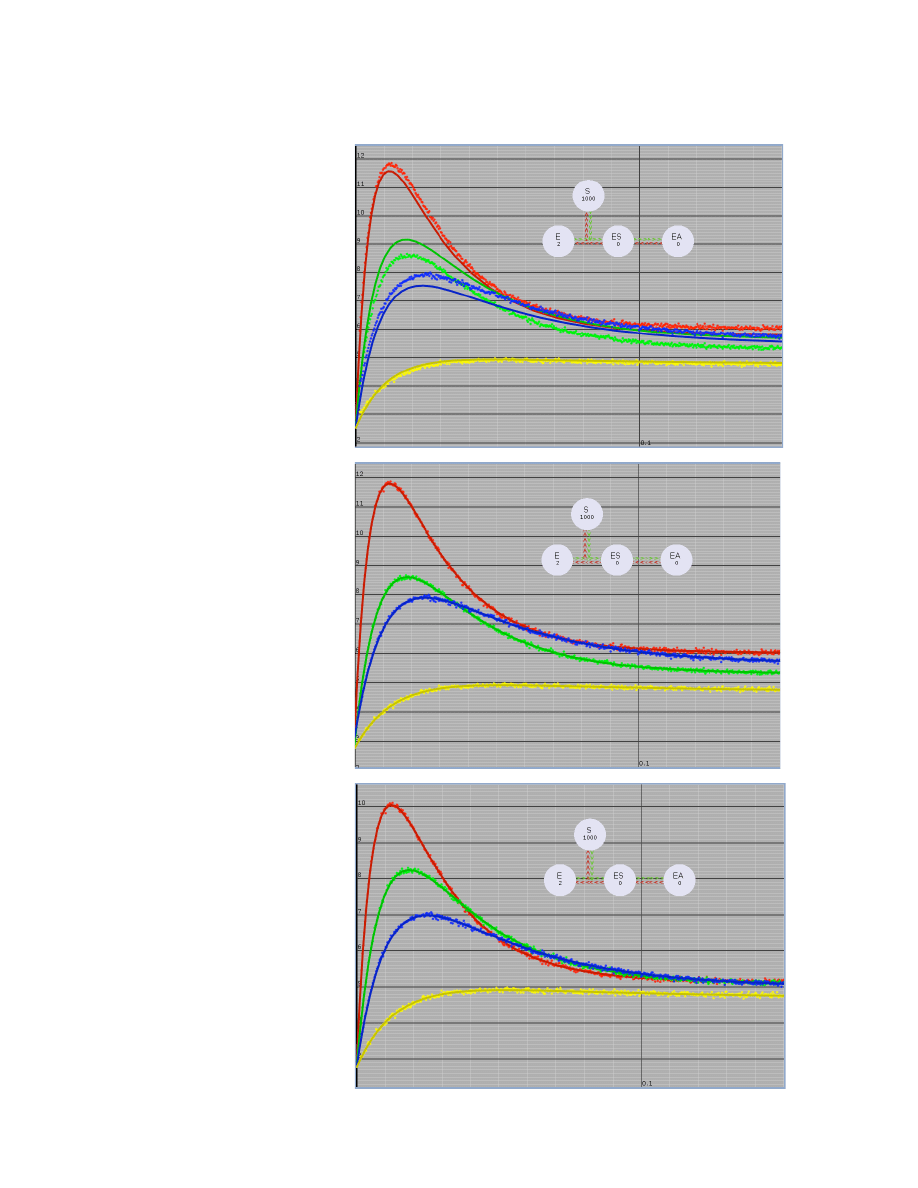
A. Data fit without normalization.
This figure shows the best fit
attainable when there are
significant fluctuations in signal
intensity for the data collected at
various concentrations.
B. Data fit with normalization. By
including a scaling factor to
normalize the fluctuations in
signal intensity, a much better fit
is obtained.
Scaling factors were derived:
Data have been scaled by factors:
scale_1a = 1.174
scale_1b = 1.044
scale_1c = 1.131
scale_1d = 1.0 (fixed)
C. Normalized Data. After
applying the normalization factors
to the data, the curves no longer
reveal fluctuations in lamp
intensity between the traces.
Data have been normalized by
factors:
scale_1a: 0.851565
scale_1b: 0.957832
scale_1c: 0.884136
These values are the inverse of
the measured scaling factors in
Figure B because these represent
the values that are multiplied by
the data during normalization.

21
Multiple-Mixing Experiments
You can program up to four mixing events. After entering the concentrations and reaction time
for the first mixing, click on
New Mix
. You then enter the concentrations of species to be added,
the dilution factor for the previous reactants (a number less than or equal to 1), and the reaction
time. See ribozyme.mec experiment #2 for an example; in this case, a fluorescent oligonucleotide
is allowed to bind in the first reaction period, and then the solution is mixed with a competing
unlabeled nucleotide in the second reaction period in order to measure the dissociation rate.
Opens a window to define the new reactant additions. Previous reactants are
diluted by the value defined by the
Dilution
term.
Plot All Mix Steps:
Show all mixing time domains when checked. The alternative is to
show only the currently selected time domain. Note also, that importing of data is controlled
by whether this button is selected. If you have data only for one time domain, show only that
time domain before importing data and the new data will be brought into that time frame.
When importing data for multiple mixing experiments, take care to display on the corresponding
reaction period prior to importing the data. The data will be imported into the displayed reaction
time period.
Importing Data
Data to be imported must be a tab-delimited text file, which can be created using a spreadsheet
program or text editor. There are several types of data files that can be imported. Once the data is
imported, it becomes part of the mechanism file (*.mec). The program computes and displays the
sum square error (SSE) in comparing the simulation with the data. In addition, the data can be fit
to the model by nonlinear regression based upon the simulation.
Note: There is no limit on the size of data files.
However, if you experience slow performance in
fitting a large number of data files with more than 1,000 - 2,000 data points per trace, you can
improve performance without sacrificing information by reducing by data averaging as the data
is imported. Enter Average N (see figure below) to establish the number of points that will be
averaged. For example if the data file has 2000 points and N=4, then you end up with a total of
500 data points, each of which was derived from the average of 4 points. We do not recommend
using this simple averaging if your data is on a logarithmic time scale.
Click to import experimental data. The data needs to be in a text file with a
default name extension of ".dat" and have tab delimited columns of data, usually with time in the
first column and then y-values in subsequent columns. Files with other extensions such as *.txt
can be opened by typing in *.txt in the file open directory search box.
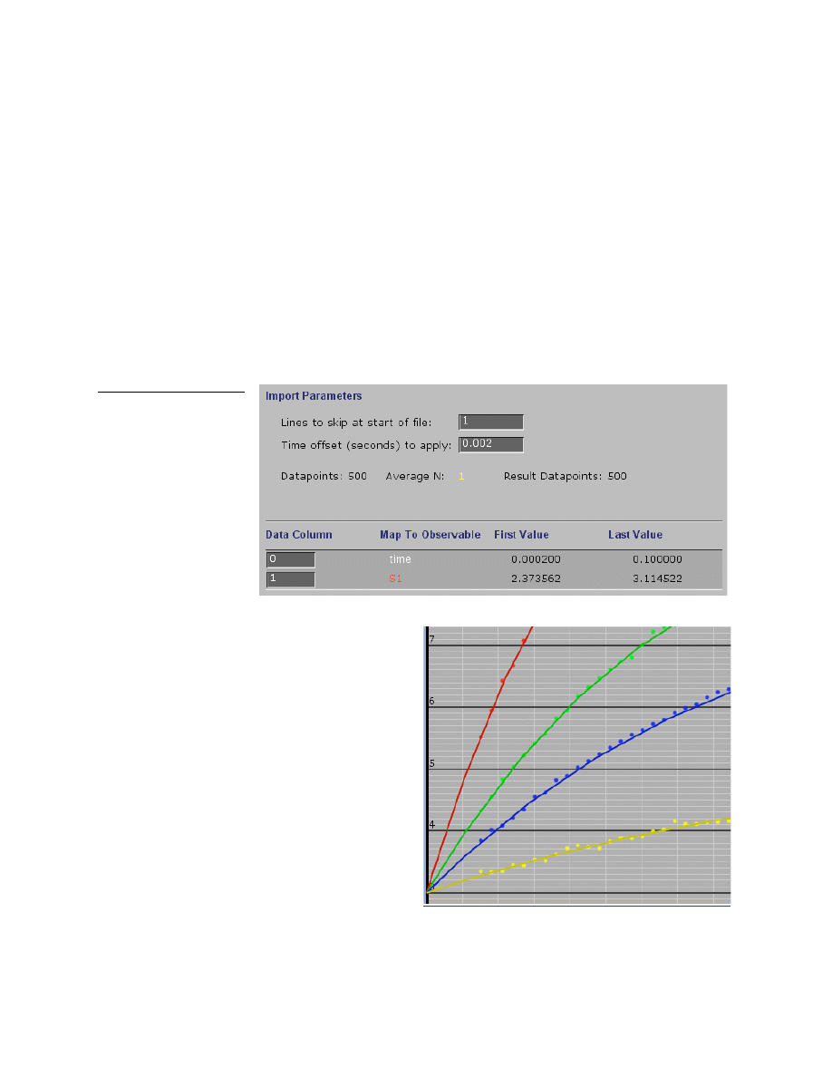
The program can be instructed to ignore a set number of rows at the beginning of the file
to read past a header at the beginning of the file. This is accomplished using the menu that
appears upon opening a new file as shown below. In addition, a time offset (such as the dead
time in a stopped-flow experiment) or the time lost in a manual mixing experiment (time
between mixing and observation) can be added to the time-axis of your data as it is imported.
Enter the delta time before clicking on Open.
22
Importing a single reaction data file
The most simple data file consists of two columns. The first column contains the time and the
second contains the Y-axis values. Labels in the first row are optional; the program can be
instructed to ignore a fixed number of rows at the beginning of a file. In creating a data file is
often useful to add labels for future reference. The figure below shows the menu when
importing this data file, time is in column 0 and the Y-values are in column 1. Note that the
program has accurately read the first and last values from each column.
The time offset can be set to correct for the dead time of the instrument, as shown in this
example where 0.002 seconds will be added to all time values. This is needed because the
simulations always start at time = 0 after mixing and amplitudes of the reaction are an important
parameter in fitting data by simulation.
Time
Y
0.0002
0.0252
0.0004
0.0034
0.0006
0.0345
0.0008
0.0029
0.0010
0.0167
...
0.0994
2.0749
0.0996
2.0827
0.0998
2.1440
0.1000
2.1180
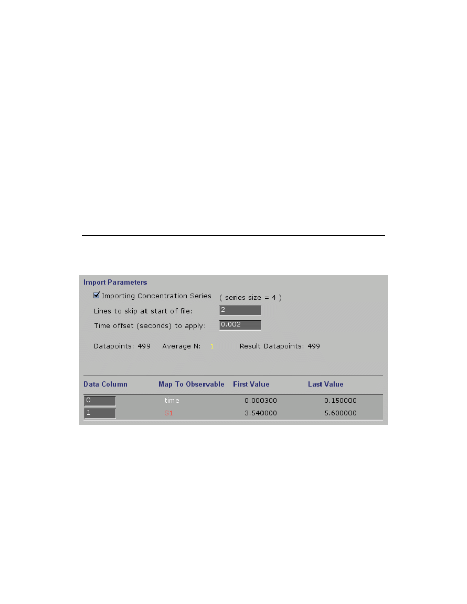
In the figure at the right, the data begin at 1.5
ms, the approximate dead time of the stopped-
flow instrument. Note how the fitted curves
extrapolate to the same starting point at each
concentration. Without the time offset, each
trace would have appeared to have begun at a
different starting point.
23
Importing data with a Concentration Series
If you have programmed in a concentration series (a set of varying concentrations for one
species), you can then import data with one time column and multiple Y-value columns as shown
by the example file shown below. This also illustrates how the first row of the file may contain
useful information, but can be skipped over by the program.
NOTE:
The concentration series must be programmed into the Experiment Editor before
importing data which includes a concentration series, and the order of the concentration series
must correspond to the order of columns of data.
Example data file showing a concentration series:
Time
0
5
10
25
50
0.0033
1.0000
1.0000
0.9997
1.0000
0.9984
0.0038
0.9998
0.9993
1.0000
0.9999
1.0000
0.0042
0.9964
0.9981
0.9989
0.9976
0.9987
0.0047
0.9937
0.9955
0.9962
0.9947 0.9956
...
3.908
0.8789
0.8414
0.8353
0.8304
0.8305
3.984
0.8793
0.8416
0.8353
0.8305
0.8304
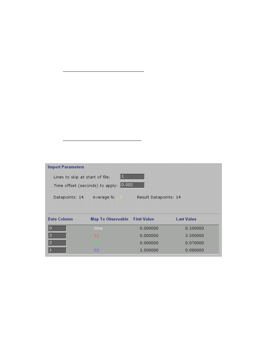
While importing this data file, the import data menu (shown below) reveals that the file is being
read properly. The program will assign each Y-value to a concentration according to the order of
values listed in the concentration series in the Experiment Editor.
24
Importing data with reactions of multiple species
In some cases you may have readings for multiple species within a given experiment such as in
the example file, EPSP_4.mec. In this case, you must correlate each species output signal (
S1
,
S2
,
S3
, etc) with a given column of data.
Example data file showing multiple species:
Time PEP
Int EPSP
0.0 3.5 0.0 0.0
0.003 2.4 0.77 0.26
0.005 2.16 0.85 0.47
0.01 1.44 0.93 1.03
0.015 1.19 0.89 1.45
0.02 0.8 null 1.9
0.025 0.58 0.58 2.32
0.03 0.5 0.43 2.54
0.04 0.33 0.35 2.84
0.05 0.2 0.21 null
0.06 0.14 0.18 3.16
0.07 0.13 0.14 3.3
0.08 0.04 0.08 3.4
0.1 0.08 0.07 3.35
This example also illustrates how the absence of a value can be indicated by the term “null.”
When parsing the file, the program will know to skip this entry. Note that the real data in the
EPSP_4.mec file does not have null values at these positions.
Note that the columns are numbered starting at zero, which is usually the time axis. Because of
the way the outputs were defined in creating the mechanism, the mapping may appear unusual:
S1
= EPSP = Column 3
S2
= Int = Column 2
S3
= PEP = Column 1

25
Generating Synthetic Data
This function generates fake data to be used in evaluating fitting to models. In
generating data, you specify the number of data points (count) and the sigma value governing the
Gaussian error added to the data such that:
σ =
1
N
(y
i
− y )
2
i
=1
N
∑
The sigma value is not a percentage error, but rather has units corresponding to the y-axis scale
and should be adjusted accordingly.
In addition, you can specify the dead time of the data collection to eliminated data shorter
than the dead time. For example, a typical stopped-flow instrument may have a dead time of 1-2
ms, so the first 0.001 or 0.002 seconds of the reaction is missed. In a hand-mixing experiment,
the dead time can be 5-10 seconds.
NOTE: To help prevent fraud, a hidden electronic signature is added to synthetic data.
Exporting Simulation Results
This function will write two text files, one containing your data and another
containing the results of the simulation in tab-delimited columns beginning with time, y1, y2,
etc. These text files can then be read into a graphics program to prepare publication-quality
figures. Two files will be output, one labeled filename.sim.txt containing the results of the
simulation and another, filename.dat.txt outputting the data, where “filename” is the name you
assign when exporting the simulation.
aFit Analytical Fitting Function
This function allows you to fit data or the simulation output to an analytical function
selected from the following list. These functions are useful in that you can do a simulation of a
complex model and then ask what rates you might have observed if you had collected data under
a given set of conditions and fit by conventional means and a defined equation. You can then use
this information to help to build you intuition and understanding of kinetics by fitting fake data,
or you can predict an appropriate model when fitting real data. Patterns for different models are
explained in [4].
Y = k*t + c
Linear function
Y = A1*exp(-k1*t) + c
1-exponential function
Y = A1*exp(-k1*t) + A2*exp(-k2*t) + c
2-exponential function
Y = A1*exp(-k1*t) + A2*exp(-k2*t) + A3*exp(-k3*t) + c
3-exponential function
Y = A1*exp(-k1*t) + A2*exp(-k2*t) + A3*exp(-k3*t) + A4*exp(-k4*t) + c
4-exponential function
Y = A1*exp(-k1*t) + k2*t + c
1-exponential burst
Y = A1*exp(-k1*t) + A2*exp(-k2*t) + k3*t + c
2-exponential burst
Y = A1*exp(-k1*t) + A2*exp(-k2*t) + A3*exp(-k3*t) + k4*t + c
3-exponential burst
26
Plot Rate versus Concentration
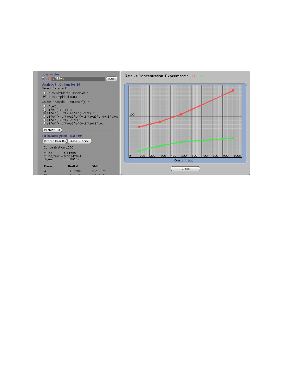
After fitting a concentration series to an analytical function, you can click on Rate v Conc and
get the display of the concentration dependence of the observed rates. The example below shows
the results after fitting the Tryp_synthase data to a double exponential, revealing the pattern for a
two-step reaction.
The example demonstrates the kinetic signature of a two step reaction in which the rates of both
steps are comparable. The slope of the fast phase provies an estimate of the second order rate
constant for the binding step (k
1
), while the maximum rate of the slow phase gives an estimate of
the sum of k
2
+ k
-2
according to the mechanism:
E
+ S
k
1
k
−1
⎯ →
⎯⎯
←
⎯
⎯⎯
ES
k
2
k
−2
⎯
→
⎯⎯
←
⎯
⎯⎯
FS
This analysis can guide you in developing a model and getting estimates for kinetic constants.
27
Data Fit Editor
Use the Data Fit Editor to:
• Fit one or all experiments
• Constrain output factors
• Normalize data during fitting
• Overlay possible fitted curves based
upon the standard error
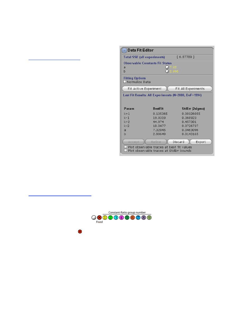
The Data Fit Editor controls fitting of data directly to a model based upon the numerical
integration (simulation) of the model. In addition to the control for whether the observable output
constants are held fixed or allowed to vary (or “float”) in fitting the data, the fitting routines also
obey the constraints placed upon the rate constants under the Model Editor.
Controlling Rate Constants
The symbols adjacent to the number controls whether an observable output factor is held fixed or
allowed to vary in fitting the data.
If the symbol is checked ( ), the output factor will not change during fitting of the parameters to
data under the Data Fit Editor. Alternatively, un-checking the control allows the output factor to
float during the fitting process. In either case, output factors can be changed manually (either by
scrolling or inputting new values).
Holding certain constants fixed, or in a known ratio provides an important constraint to
achieve a meaningful fit to the data. Alternatively, rate constants can be grouped so they
maintain a constant ratio with respect to other members of the group. See Model Editor for more
details.
28
Fitting Experiments to the Model
Fits only the currently selected experiment
Globally fits all of the experiments in the current .mec file.
In either case, the program performs nonlinear regression to find the best fit for all parameters by
fitting directly to the model based upon numerical integration of the rate equations and the
starting conditions for each experiment. The program will iteratively seek the minimum sum
square error for all data.
Normalize Y-Axis in fitting multiple experiments:
This function is useful when fitting
multiple data sets with greatly varying Y-axis ranges. To normalize the data during the fitting, all
experiments are scaled on a range of 0-1. This prevents data with a larger Y-axis range from
dominating the global fit. This function is distinct from the normalization of traces within a
concentration series, where a scaling factor is derived for data within a single experiment. In this
case, the Y-axis is scaled only during the fitting process in a manner that is transparent to the
user. After the fitting, the data are plot on the user-defined scale. See the example file:
Flour_&_quench_data.mec which illustrates need for this normalization. The Y-axis of the
quench-flow data spans the range of 0-1000 while the fluorescence data is on a scale of 0-1.5.
After fitting, the graph will display the fit in gray in addition to the colored output for the starting
parameters, and several new buttons appear.
Accept, Reject or Refine.
The results of the fitting are copied to your working model.
When you click Refine, the program will accept the results of the last fitting, then
run the fitting routine one more time, starting with the new values derived from the previous
round of fitting. Each time you click Refine, the process will repeat and you will see the best fit
parameters update. Re-starting the fitting process involves a re-initialization of parameters that
control the nonlinear regression in ways that are transparent to the user, and allows the fitting to
be refined. Usually, this does not change the fit significantly.
Reverts to the previous model parameters.
Plot observable traces at best fit values:
This turns on and off a thin black line showing the
best fit.
Exporting Fit Results
Press Export to save a text file containing a summary of the fitted parameters and
standard error. Additional statistics are also given, including the covariance matrix.
Text files suitable for generating publication-quality graph of each experiment can be exported
using the function Export Sim under the Experiment Editor.
29
Plotting Confidence Intervals
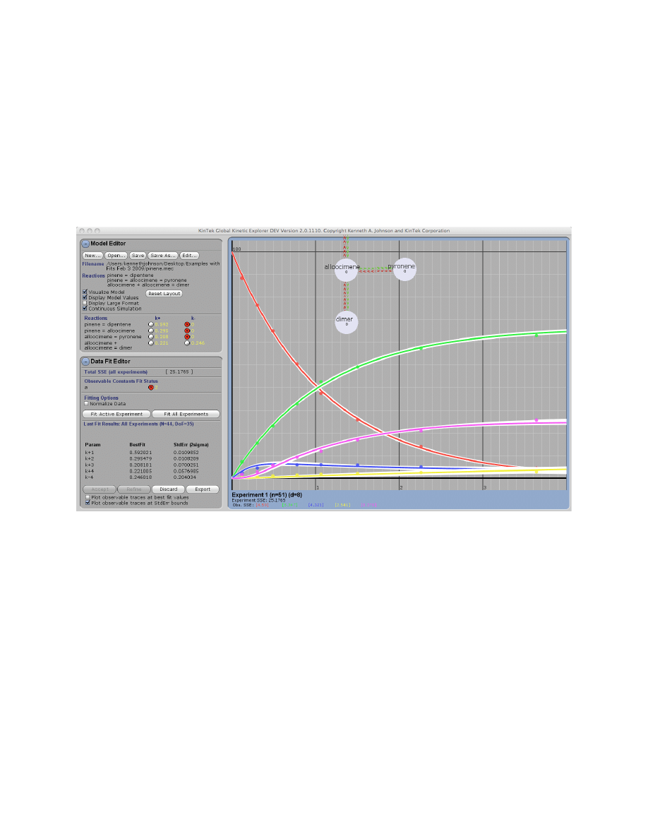
Plot observable traces at StdErr bounds:
This turns on and off an overlay of all possible fits to
the data obtained by generating curves based upon the extremes of parameter values based upon
the standard error. For each upper and lower bound of each variable parameter, the program will
find the combination of all parameters yielding the best fit for each individual parameter extreme
as shown below (pinene.mec example). The white lines show the range curves attainable for the
limits of error on all fitted parameters. For example, curves are generated for k
+1
= 0.60 and k
+1
=
0.62 based upon the estimate of k
+1
= 0.59 ± 0.01
µM
-1
s
-1
. For the curve at k
+1
= 0.60, the data
are fit again allowing other parameters are allowed to float in finding the best fit for that
parameter extreme, the plotted on the graph. The process is repeated for each variable parameter.
This analysis is useful in that it shows the extent to which fitted curves are thought to be
constrained according to the standard error. Examine each of the examples to understand the
relationships. In some cases, when parameters are not well constrained by the data, you will see
overlaid traces that are indistinguishable from the best fit (i.e., racemase_3step.mec). In another
case, dynein.mec, the ATP binding rate is constrained only to 8 ± 3.7, the overlay reveals the
limitations in the data that prevent tighter limits on k
+1
.
NOTE:
The FitSpace calculation, described below, produces cleaner displays of overlay traces
because it overcomes many of the limitations of computing standard error when parameters are
not well constrained.
Error Analysis
Data fitting by nonlinear regression produces a standard error estimate based upon the
covariance matrix [5; 6]. We are convinced that this error analysis is extremely misleading when
applied to multiple variable fitting and one should exercise caution in interpreting the standard
error analysis produced during data fitting. For example, in the racemase.mec file you will note

30
that fitting suggests that k
-2
= 6.45 ± 0.03 x 10
8
s
-1
. (sum square error = 873.7) However, if k
-2
and k
3
are scrolled downward by 5 orders of magnitude, one then gets k
-2
= 9070 ± 67 s
-1
(sum
square error = 872). Thus, k
-2
is not well determined at all. This is readily revealed using the
Dynamic Simulation and by the FitSpace analysis described below and in our recent publications
[2; 3].
Users are encouraged to explore the range over which parameters can vary by scrolling
individual constants or pairs of linked constants and monitoring the visual appearance of the
curves and the sum square error calculations, thereby taking advantage of all that the Dynamic
Simulation has to offer. Exploration of the landscape after fitting using the Dynamic Simulation
will do much to tell you about the range over which a given rate constant can be varied. Also,
think carefully about the model and use the ability to link rates in a constant ratio to explore the
multi-dimensional fitting landscape without perturbing the net equilibrium constant. Note, for
example, that there are large changes in the simulated curves and the sum square error if k
-2
in
racemase.mec is varied individually. This is because the equilibrium constant is thrown off.
However, if k
-2
and k
3
are linked and varied in synchrony, the full range over which they can be
varied is revealed.
Fitting data to a model is often difficult because one needs to include all steps in a
pathway even though some rates may not be known. Therefore it is important to recognize which
rates are constrained by the data and which are not. In particular, it is often the case that a rate
constant for a given step may only have a lower limit because as long as the rate is greater than
that lower limit, it may not matter what the rate is. This situation is typical when a model is
under-determined. In fact, the appearance of a rate, which is much faster than neighboring rates
in a reaction sequence, should be taken as a red flag indicating the model may be overly
complex, as in the racemase.mec example.
In a separate section below, we describe computation and use of FitSpace to evaluate the
extent to which parameters are constrained by the data.
Summary of Steps in Fitting Data
1. Prepare text files containing data following one of the three patterns described under
Importing Data. If the concentration of a single species is varied across a family of
curves they can all be in one file; alternatively, if different data sets involve changing
more than one species, they must be in individual files, each given as rows of x,y pairs.
2. Decide on an appropriate mechanism and create or copy a mechanism file, then enter
estimates for rate constants. At this stage, prior fitting by conventional methods may
provide important clues to suggest the model and provide estimates on rate constants.
Conventional data fitting is useful in that it isolates and illustrates trends in the data that
reveal the underlying mechanism.
3. In KinTek Explorer, define one “experiment” to correspond to the conditions used to
collect data in each individual data file. Define the output functions that correspond to the
signal of observables for each experiment.
4. Import the data for each experiment setup. During data import, the program matches the
data to a given simulation output. Therefore, it is necessary to define the simulation
before importing data. If you have data covering a concentration series (a series of
experiments performed over the same time scale at several concentrations on one
species), then the program will assume that the order of the series in the experiment setup

31
corresponds to the order of columns in your data file. Be careful at this point to match up
the data with the simulations.
5. Adjust rate constants and output factors in attempting to mimic the data. At this stage of
the fitting, you can begin to get an idea of which rate constants may be determined by the
data and which might not. Fix any rate constants that are known from other experiments
and not established by the current experiment. Look for pairs of rate constants that might
be linked.
6. Fit the model to the data using the automated functions under Data Fit Editor.
7. Explore the range over which parameters can vary by scrolling individual rates or pairs of
constants while monitoring the output. Try moving parameters into new ranges and fit the
data again; this can be done by fixing the new rate or allowing it to float. This may be the
most important part of the fitting process where you can use the dynamic simulation to
explore the extent to which individual constants are constrained by the data.
8. Critically evaluate your model and your fit to the data. Can the data be fit equally well to
a model with fewer steps? Edit the model and seek the simplest model to explain your
data by including only those steps that are well constrained by your data. If steps must be
included for which there is no information to define their rates, provide minimal
estimates for the magnitude of the rate constants and clearly identify them as such in all
publications. There is nothing wrong with stating that a given rate was set at a given
lower limit because the data did not constrain it to a known value. In particular, it is often
necessary to assume a diffusion-limited collision rate (typically 100 µM
-1
s
-1
), but clearly
state the assumption.
CAUTION!
The real danger in fitting data globally to a model is in trying to convince yourself
and your colleagues that a model is well-determined when it is not. Such overstatements of the
utility of global fitting actually undermine confidence in the method. You do not get something
for nothing simply because you fit your data globally. The information content of the data still
limits the conclusions that can be made. What you do gain is that the data are interpreted more
rigorously and that more of the information content (particularly amplitude information) can be
extracted from the data, and assumptions necessary for mathematical solutions can be avoided.
Dynamic simulation was implemented in designing KinTek Global Kinetic Explorer so
that you can see the relationships between the rates, the model and the data. Take advantage of
the powerful method to fully explore the fitting landscape, critically evaluate your model, and
carefully state your conclusions. In the next section, we present our methods to explore the
fitting landscape through our FitSpace function.
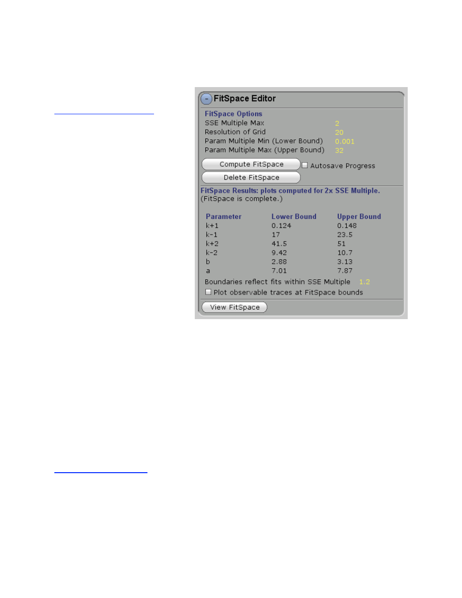
32
FitSpace Editor
Use the FitSpace Editor to:
• Set parameters limiting the
Fitspace search
• Compute Fitspace
• View Fitspace
•
Set the SSE boundary error
estimation
•
Plot traces to display the err
limit boundaries
In our data fitting routines described above, standard error analysis is based upon the covariance
matrix resulting from nonlinear regression. The standard errors reported using these methods
always understand true experimental errors because the methods are based upon the assumption
that all errors are independently and identically distributed; often this is not the case because
there are bumps in data or non-uniform variation from ideal behavior. Moreover, in many cases
standard errors are extremely misleading and imply a well-constrained fit, when, in fact, there is
a large space over which parameters can vary. Here we make an important distinction. If the
nonlinear regression converges to produce a fit to the data, it can be described as a good fit in
that the errors have reached a minimum. However, this does not mean that the parameters are
well-constrained and that the fit is unique. In the computation of FitSpace, KinTek Global
Kinetic Explorer allows you to explore the landscape over which parameters can vary while still
achieving a good fit to the data. This is described in more detail in our recent papers [2; 3].
Confidence Contours
In principal, one would like to examine the data fitting landscape in n+1 dimensions, for
n independent parameters. Because that is not possible, we examine parameter in all possible
pair-wise combinations to examine the extent to which any two parameters can co-vary and
produce a good fit, as judge by the sum square error. To begin the exploration of FitSpace, the
program steps through each variable parameter (rate constant or scaling factor) and holds it
fixed, while allowing all other variables (selected by the user) to float as nonlinear regression
seeks the best fit. The process is repeated until the range of each parameter is mapped. We then
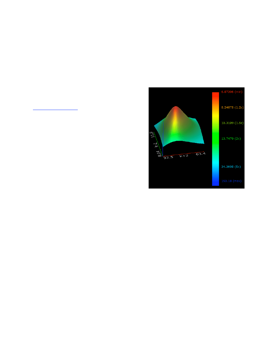
33
plot a 3D graph showing the dependence of the reciprocal of the normalized sum square error
versus each parameter pair (x, y axes) as shown below. That is, at each x,y pair on this grid, the
sum square error (SSE) is calculated for the best fit, attained by allowing all other parameters to
be adjusted. We then plot the SSE
min
/SSE
x,y
on the vertical axis so that it falls on a scale of 0 to
1, with 1 being the best overall fit. The color coding and the scale on the right gives the absolute
sum square errors calculated. This example shows clearly that the rate constants k
+2
and k
-2
in the
model are well-constrained. The process is repeated for all of the pair-wise combinations of
variable parameters to generate a graph as shown on the following page, derived from the
tryptophan synthase example [1].
Confidence Contour.
The figure at the right shows
the 3-dimensional surface generated in
computuing the normalized best-fit SSE function
as k
+2
and k
-2
are systematically varied in the
Trypsynthase.mec example.
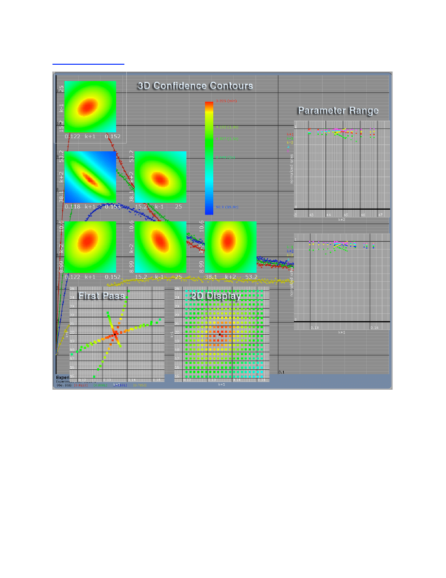
34
FitSpace Display
FitSpace Display:
First Pass shows the results the initial excursions to map the boundaries of a good fit.
2D Display shows the grid of x,y pairs obtained from a stepwise grid search.
Parameter Range shows the dependence of all parameters on each forward rate constant that
was allowed to vary. On this graph, each point represents a parameter that produced a fit
within 10% of the minimal SSE. The parameters are normalized to their maximum value.
Note the parameters are clustered within 0.8 to 1, implying that in this example, the
parameters are well constrained. Contrast this display with that shown on the following page.
3D Plots region show the 3D representation of the SSE variation for each pair of rate
constants. Note that each pair of rate constants is well constrained with a well-defined local
minimum. The ridge in the relationship between k
+2
and k
+1
indicates that the product k
+1
*k
+2
is more constrained that either value individually.
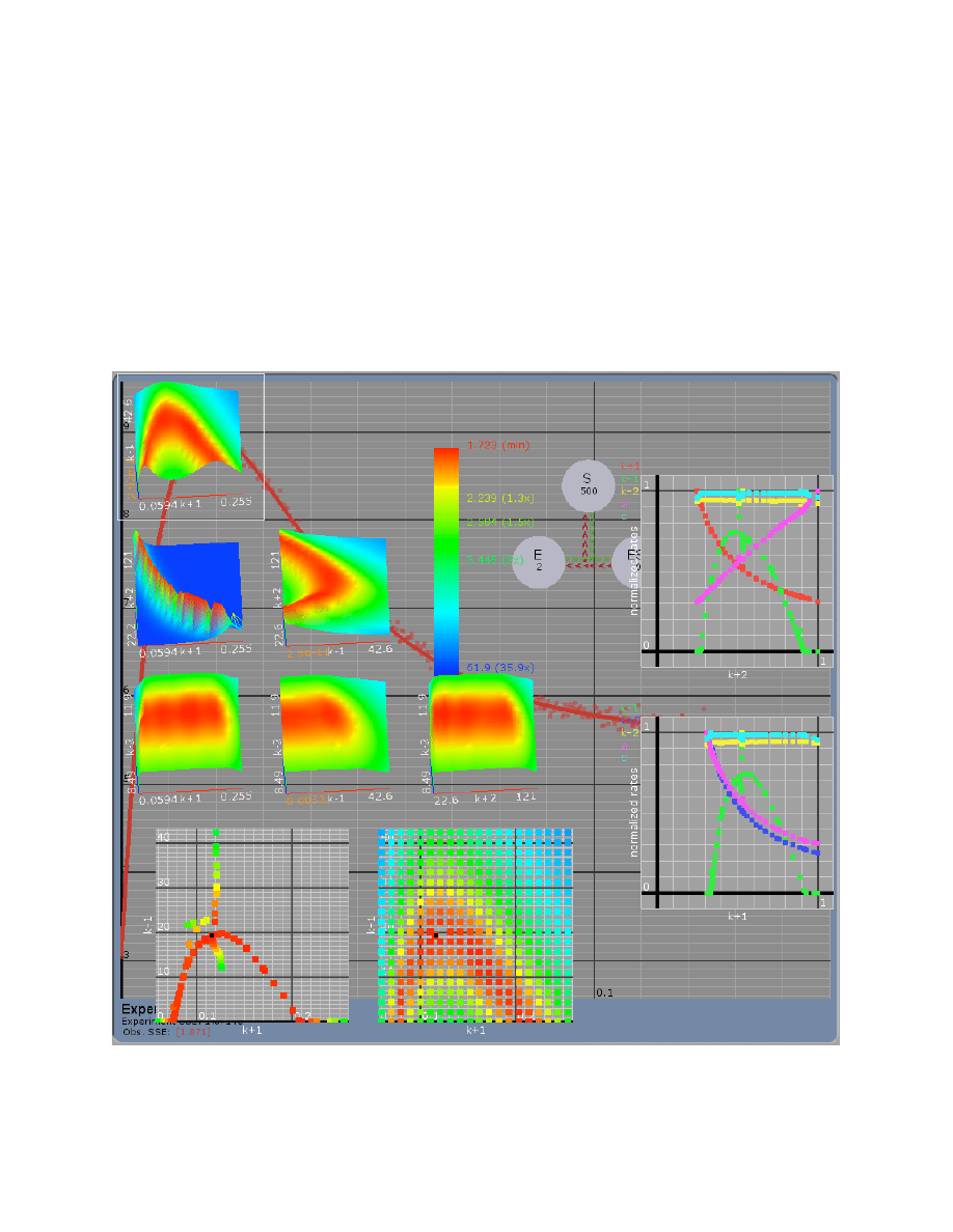
35
The data contained in the tryptophan_synthase.mec file provides well-constrained estimates for
all six parameters, consisting of four rate constants and two fluorescence-scaling factors. The
well-constrained fit for the tryptophan synthase data is dependent upon the concentration series.
It is the concentration dependence of the rate and amplitude of the fast and slow phases as well
as the starting and ending points that allows definition of 6 parameters. To illustrate this, we
show the results of a FitSpace calculation where data from only one of the concentrations is
included. In this case, the parameters are clearly not well constrained. Note especially that there
is no lower limit for k-1, while the other parameters can vary over a wide range of values, as
evidenced by the Parameter Range plots as well as the shape and range of the 3D plots. These
two examples illustrate how the FitSpace calculation gives immediate visual clues to indicate
whether a fit to a data set is well constrained or not.
Note that the 3D graph for k
+2
versus k
+1
shows an extended ridge defining a function k
+1
*k
+2
=
C, a constant. Because of the grid sampling, this appears as a series of peaks, but it is a
continuous function.
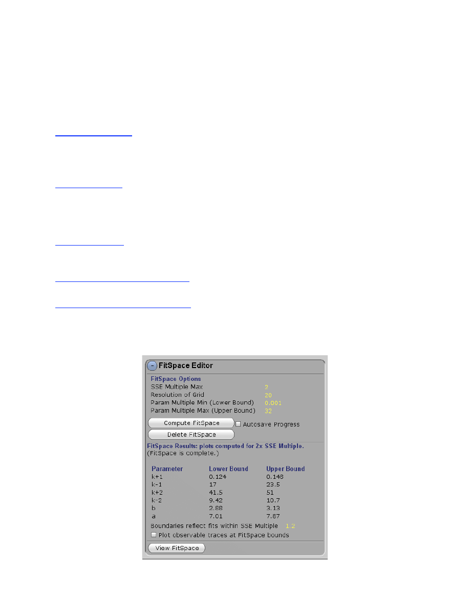
36
Examination of the FitSpace contours can provide more reliable error estimates on individual
parameters than given by conventional nonlinear regression analysis. A given threshold of the
normalized SSE values can set a boundary to define the acceptable limits or a given parameter.
As a visual cue, the orange/yellow boundary represents a 30% increase in SSE and may represent
a reasonable boundary for acceptable fits to the data. We use this boundary to provide estimates
for upper and lower bounds on parameters, given in the table under FitSpace Options.
FitSpace Options
This section describes how to run a FitSpace calculation and control display of the output. After
a fit to a data set is achieved, you can simply click on Compute FitSpace to begin the calculation.
Three parameters can be set to control the computation:
SSE Multiple Max:
range 0.1 to 10, default 2.0. This factor sets the limit on the variation in SSE
as the program searches the space over which a parameter can be varied. For example, when set
to 0.6, the program stops searching when the SSE exceeds 60% of the minimum value. A smaller
number provides better resolution around the boundary and also limits the search when
parameters are not well constrained. A larger number allows a broader search.
Resolution of Grid:
range 5-20, default 10. This parameter sets the resolution of the grid search;
for example, a value of 10 give a 10x10 grid. Higher numbers give smoother 3D graphs but
require more computation time.
Param Multiple Min (Lower Bound):
range 0.0001 to 1, default 0.001. This parameter sets a limit
on the fold variation in a parameter before the program stops searching for a lower boundary.
Param Multiple Max (Upper Bound):
range 1-100, default 32. This parameter sets a limit on the
fold variation in a parameter before the program stops looking for an upper or lower boundary.
For example, if a parameter has no upper boundary in that increases in the value of the parameter
do not increase SSE, then the program will stop when the variable exceeds 100-fold the starting
value.
37
After the Fitspace computation is complete, the table showing upper and lower bounds of each
parameter appears. This is based upon the threshold set in SSE; a threshold of 1.2 represents a
20% increase in SSE.
This toggle controls the display of the FitSpace graphs.
The results of a FitSpace calculation are stored with the
*.mec file and can be reviewed pressing View FitSpace.
This pair of buttons allows the user to scroll through the
individual 2D plots.
Toggles the FitSpace display through several options.
Use boundary samples in 3D plots
. This checkbox allows additional points obtained in
searching for boundaries of acceptable fits to be added to the 3D contour plots.
Lighing.
This checkbox toggles on and off the side lighting of the 3D plots.
Grayscale.
This checkbox toggles between colored and grayscale version of the 3D plots.
Solid Backdrop.
This checkbox toggles between a black background and a grayed version of
the data screen.
Mouse Control
:
By clicking on one of the 3D plots with the middle mouse button and dragging
the mouse, the angle of the 3D view can be changed to see the contours more clearly.

38
Errors on fitted parameters
The FitSpace calculation allows more reasonable estimates of errors on the parameters than are
achieved by conventional nonlinear regression. However, it should be noted that this is an area of
less than exact science. We all take comfort in reporting the 95% confidence intervals from the
nonlinear regression, but the standard errors always underestimate the true error, sometimes to a
large extent.
FitSpace Boundary Error Limits
Boundaries reflect fits with SSE Multiple X:
This scrollable parameter sets a threshold on the
FitSpace confidence contour for computation of the ranges allowed for fitted parameters. Note
that as you scroll the value, the color boundary on the 3D plots changes to show the new
threshold as the yellow boundary between red and green (or the edge of the white center in a
grayscale rendition). After you release the mouse button, the table showing Lower and Upper
Bounds will be updated. For most experiments a threshold of 1.1 gives a reasonable range for
errors. With thousands of data points that are independently and identically distributed, a value
of 1.01 to 1.1 may be appropriate. With only 40 data points, a value of 1.35 may be more
appropriate. In a future release of the software, a recommended threshold will be calculated.
The table below illustrates the problem based upon error analysis on parameters derived
in fitting the tryptophan synthase sample data. According to the nonlinear regression, each
parameter is known within less than 1% error. However, the FitSpace shows that several of the
parameters can vary over a much larger range. In particular, k
-1
, should be reported as 20
± 5,
which is a more realistic estimate and 19.9
± 0.37
Parameter
Best Fit
Std Error
Lower Bound
Upper Bound
k
+1
0.135
0.001
0.128
0.144
k
-1
19.9
0.37
16
25
k
+2
45.1
0.46
42.8
46.5
k
-2
10.0
0.072
9.5
10.7
a
7.33
0.046
b
3.00
0.014
A more troubling example is shown in the racemase.mec file. Nonlinear regression
reports that k
+3
= (2.55
± 0.044) x 10
9
s
-1
and k
-2
= (6.6
± 0.17) x 10
8
s
-1
. However, FitSpace
exploration and dynamic simulation each reveal that these constants are not well constrained at
all. They are bounded on the lower limit only by k
cat
in each direction, while there is no upper
limit for either parameter.
Note added January 23, 2009: Recent improvements in data fitting, principally due to
performing all calculations in double precision (64 bit), have overcome some of the problems
with error estimates derived by nonlinear regression when systems are under-constrained. In
particular, the current version of the software (Version 2.0.1059) returns errors for the
racemase_4step.mec of k
+3
= (2.44
± 0.63) x 10
9
s
-1
and k
-2
= (6.64
± 6.3) x 10
8
s
-1
. Although this
represents a significant improvement in dealing with situtations where error terms are large,
nonlinear regression standard errors may still fail to reveal the full extent to which parameters
are under-constrained.
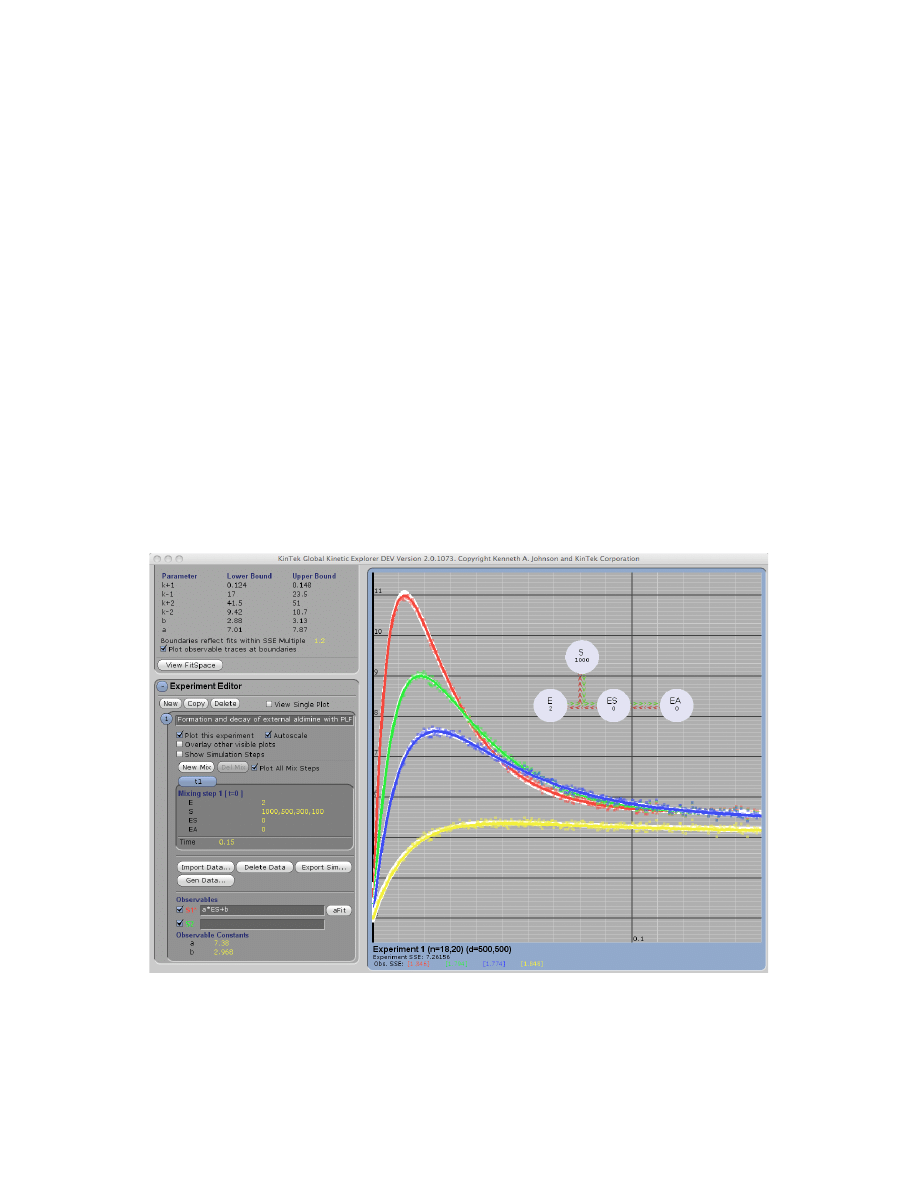
39
Plotting Confidence Intervals
We have added a new function to show the overlay of all possible fitted curves within the
boundaries defined by the FitSpace confidence contour threshold.
Plot observable traces at boundaries:
This option appears after completing a FitSpace contour
analysis. When this item is checked, all of the reasonable fits to the data will be overlayed with
the data and the best fit as shown below. The curves are computed based upon the parameter sets
defined by the lower and upper limits of each variable parameter according to the value set for
“Boundaries reflect fits within SSE multiple x”, where x is the user input value for the threshold.
After the threshold is changed, the display is updated if the Plot observable traces at boundaries
function is checked. It is important to note that these curves are not simply the taces obtained by
varying a each parameter individually while keeping all other parameters fixed at their best fit
values. Rather, for each overlayed trace one parameter is set to its upper or lower limit, while all
other parameters are adjusted to display the best fit attainable within the set SSE threshold. The
process is repeated for the upper and lower limits of each variable parameter to overlay the
family of acceptable traces (in white) behind the data and the best fit (in color). For comparison,
consider the examples such as 8oxodG.mec, where there are fewer points to define the
parameters as accurately, although they are still well constratined; and racemase_3step.mec,
where the parameters are totally unconstrained (except for lower limits), yet all of the traces
superimpose on the data. This function provides one more tool to evaluate the relationships
between the data and allowable range on the fitted parameters.
Display of observable traces at parameter boundaries. This figure shows the display all
reasonable fits to the data obtained for Tryp_synthase.mec within a SSE threshold of 1.2.
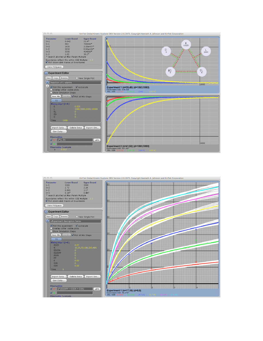
40
Display of observable traces at parameter boundaries. This figure shows the display all
reasonable fits to the data obtained for Racemase_3step.mec within a SSE threshold of 1.2. Note
the wide range of the parameters used to generate the plots shown here.
Display of observable traces at parameter boundaries. This figure shows the display all
reasonable fits to the data obtained for 8oxodG.mec within a SSE threshold of 1.2.

41
Appendix
Example Files
Here we present example files that illustrate the fitting routines and the use of dynamic
simulation to evaluate models. We welcome additions to this list. If you have a data set that you
would be willing to include, please send it to kajohnson@kintek-corp.com along with references
that we should include in citing your work.
8oxodG.mec This mechanism file shows data collected on the incorporation of 8-oxo-dGTP by
the human mitochondrial DNA polymerase and the fit to a model with slow pyrophosphate
release [7].
Actin_Isomerization.mec This mechanism provide a good example to illustrate the extent to
which conventional nonlinear regression underestimates errors on parameters. Nonlinear
regression returns standard errors indicating approximately 10-18% error on k
1
and k
-1
. However,
FitSpace analysis shows that the data only place a lower limit on k
1
= 0.002 and define the ratio
K
d
= k
-1
/k
1
= 990 ± 40
µM. You can confirm this by linking k
1
and k
-1
, then scrolling to see the
allowable range of variation in k
1
and k
-1
. Also try fitting and computing FitSpace with various
combinations of either linked or fixed values of k
1
and k
-1
.
Actin_polym.mec The kinetics of actin polymerization are modeled as described by Freiden [8]
where spontaneous initiation is a function of several weak oligomerization steps. Note that his
model is valid only when polymerization is favored; otherwise, the species F becomes an infinite
source of actin monomers during depolymerization.
Actomyosin.mec This complex model shows the simulation of several experiments to mimic
stopped-flow fluorescence and light scattering data for actomyosin and myosin ATPase [9].
Alcohol_dehydrogenase.mec In this mechanism, de-protonation of horse liver alcohol
dehydrogenase-NAD+ complex controls formation of the ternary complex [10]. Data are from
Fig. 5, and the mechanism and rate constants are in Table 3, with the output factors from Table 4
as described the Experimental Procedures section (for effective buffer concentrations and
apparent extinction coefficients). Only 9 data sets are included, but the original fitting included
28 data sets. Special thanks to Bryce Plapp (Univ. of Iowa) for providing this file.
Binding_data1.mec and binding_data2.mec These files provide data that has not yet been fit.
As an exercise in data fitting, will need to redefine the output factors and/or the mechanism fit
these data.
Binding_onestep.mec, Binding_rapidequil.mec, Binding_reversible.mec,
Binding_twostep.mec These example files illustrate the various kinetics that one can observe
with simple binding reactions.
Burst_irrev. mec A simple pre-steady state burst of product formation is shown for the case
when the chemistry step is irreversible.
Burst.mec This shows a simple pre-steady state burst of product formation, with each of the
species illustrated. A typical burst is given by the sum of EP + P.

42
Burst_with_Fluorescence.mec In this model, a possible fluorescence trace is displayed as the
weighted sum of enzyme species. Note how the shape of the curve changes as output factors f1,
f2 and f3 are changed; although the observable rates of reaction will not change, there are
circumstances under which it may be difficult to resolve the two rates. Use the “aFit” function to
see what rates would be obtained by conventional fitting to each of the traces.
DHFR-binding.mec The time dependence of a protein fluorescence change observed when
binding tetrahydrofolate to dihydrofolate reductase is shown, along with a competition
experiment to measure the dissociation rate observed after mixing with methotrexate. The
synthetic data were generated to mimic the results reported by Fierke et al. [11].
DHFR.mec This is a complex model showing the reaction pathway catalyzed by dihydrofolate
reductase and simulation of several experiments as reported by Fierke et al. [11].
Dynein_burst.mec Two rapid quench experiments are shown, performed at two different ATP
concentration, for the dynein ATPase. The red trace shows the results of a pulse-chase
experiment to measure ATP binding, while the blue trace shows the results of an acid quench to
measure ATP hydrolysis. Fitting the data simultaneously provides estimates for rates of ATP
binding and hydrolysis as well as the reverse of hydrolysis at the active site. Note the lag in the
time course of ATP hydrolysis, determined not by the acid quench-date, but required by the time
dependence of ATP binding [12]. Also note that the pulse chase is modeled as a*EA + EP + P
because bound A continues forward to form product during the chase period with a partition
coefficient determined by a = k2/(k2 + k-1). In the dynein_burst.mec, a = 49.3/(49.3+2.78) =
0.95 so this is a small correction factor. You have to solve for a manually by iteratively fitting
data, computing a, and then fitting data again.
EPSP.mec This contains four experiments performed on the enzyme, EPSP synthase. In these
experiments, rapid quench-flow methods afforded the direct observation of an intermediate
formed at the active site of the enzyme. Fitting is constrained by known equilibrium constants for
steps 1, 3, 4, and 6 in the reaction sequence. For example, note how k
3
and k
-3
are linked to give
K
3
= 12. In addition, the overall equilibrium constant is 180 [13]. Use the dynamic simulation to
show that the data set a lower limit on k
3
but not an upper limit.
EPSP_glyphosate_binding.mec This file shows both the glyphosate and S3P concentration
dependence of the fluorescence change that occurs after both S3P and glyphosate bind to EPSP
synthase.
Fluor & Quench Data.mec This file contains data simulated to mimic experiments obtained by
stopped-flow fluorescence and rapid quench-flow methods and illustrates the use of normalizing
data in fitting data that have markedly different Y-axis scales. If you attempt to Fit All
Experiments without normalization, the fit is dominated by the quench-flow data. However, if
you check “Normalize Data” then the global fitting weights each experiment equally.
HIV_NNRTI.mec This file contains data showing the effect of nonnucleoside inhibitors
(NNRTI) on DNA polymerization catalyzed by HIV reverse transcriptase [14]. This file
illustrates the use of double mixing where the slow-binding NNRTI is first pre-incubated with
the enzyme-DNA complex before adding nucleotide to begin polymerization.

43
Kinesin-mantADP.mec Kinesin with mantADP bound to two sites was mixed with
microtubules at various concentrations of ATP, ranging from 0 to 150 µM. The decrease in
fluorescence provides a signal for the release of mantADP from the kinesin. The reaction is
biphasic. The fast phase is due to the release of mantADP from the first site and is independent
of ATP concentration. ATP binds to the open site, stimulating the rate of release of mantADP
from the second site. Simultaneously fitting the family of curves defines the rate of ATP binding
and the rate of release of mantADP from the M-K-ATP-mantADP complex. These data provide
direct evidence for an alternating site ATPase in which the binding of ATP to one site stimulates
the release of product (ADP) from the neighboring site [15; 16].
Myosin.mec This illustrates the simultaneous fitting of stopped-flow fluorescence and rapid
chemical quench-flow data based upon the work by Johnson and Taylor [12]. The file contains
synthetic data to mimic that shown in the original publication. By simultaneously fitting the two
data sets, the correlation between the second fluorescence change and the rate of the chemical
reaction is established much more definitively than by simply overlaying the two data sets. In
addition, one should note that the first very fast conformational change (k
2
) was based, in part,
on the loss of signal amplitude in the stopped-flow. Global fitting places a lower limit on k
2
by
including the amplitude information.
PBP_PPase.mec Data supporting a coupled fluorescence enzyme assay are shown in which
pyrophosphatase hydrolyzes pyrophosphate and the resulting phosphate binds to a fluorescently
labeled phosphate binding protein to provide a signal [17; 18; 19].
Pinene.mec The time dependence of the thermal decomposition of
α-pinene is shown with a fit
to a simple model [20]. These data have provided a challenging example for fitting data by
nonlinear regression to analytical functions [5; 6], but are handled easily using KinTek Explorer.
In that example as described in the textbooks, the reaction involving dimerization of alloocimene
was assumed to be unimolecular in order to derive an analytical solution to the rate equations!
Fitting by numerical integration overcomes this severe limitation and provides a meaningful rate
constant for the dimerization reaction. This is described in more detail in our paper on the
KinTek Explorer simulation program [2].
PNPase-Hs-ImmH.mec and PNPase-Pf-DADMe-ImmH.mec. Immucilin-H is a slow tight
binding transition-state analog inhibitor of purine nucleoside phosphorylase. These files show the
time dependence of product formation after mixing enzyme with substrate and various
concentrations of Immucilin-H [21]. PNPase-Hs-ImmH.mec shows results for the human
enzyme, while PNPase-Pf-DADMe-ImmH.mec shows results for the enzyme from Plasmodium
falciparum (malarial parasite). The example files show how relevant parameters can be obtained
by global fitting. In fitting the data the challenge is to establish the errors on individual
parameters and to define which parameters are well constrained. Compare the global fit to the
results obtained by fitting to a burst equation. Immucilin-H is now in clinical trials as a
treatment for T-cell leukemia. Special thanks to Andrew S. Murkin and Vern Schramm (Albert
Einstein College of Medicine) for providing these data.
Pol_burst_series.mec To study DNA polymerization, an enzyme-DNA (ED25) complex is
mixed with nucleoside triphosphate (N) at various concentrations and the burst of product
formation is measured (resolving DNA 25 nucleotides in length from DNA 26 nucleotides in
length on a polyacrylamide gel). The family of curves can be fit simultaneously to extract the
ground-state binding constant for binding dNTP and the maximum rate of polymerization. In this
example, the rates of binding and dissociation of each ED complex is included for completeness,
but the rates are constrained from known values.

44
Pol_processive.mec To study processive DNA synthesis by a polymerase, an enzyme DNA
complex is mixed with a solution containing 3 of the nucleoside triphosphates, which according
to the DNA sequence of the template leads to sequential incorporation of 5 nucleotides. Analysis
of the time dependence of the appearance and disappearance of each intermediate species can be
fit to obtain estimates for the rate of each elongation step.
Progress_curves.mec This file illustrates synthetic data for a minimal set of experiments to
define k
cat
, K
m
and K
i
for product inhibition from analysis of a full time course (progress curve)
of enzyme catalysis. Note that the substrate and product binding rates (k
1
and k
-3
, respectively)
are fixed at 10
µM
-1
s
-1
in order to reduce the number of variables to correspond to the
information content of the data. The kinetic parameters obtained by fitting allow computation of
k
cat
and K
m
in both the forward and reverse directions, but do not allow definition of intrinsic rate
constants. Note also that this example shows that a single progress curve is not sufficient to
define the mechanism; one trace can be fit adequately to a simple k
cat
, K
m
model with irreversible
reactions (ignoring product rebinding and reversal of chemistry) but the concentration series
cannot be fit to such a simple model. Thus, when fitting real data and no knowledge of the extent
of product inhibition (reaction reversal), one cannot reliably fit to a the progress curve obtained
at a single concentration of substrate.
Question_1.mec, Question_2.mec and Question_3.mec These contain data files corresponding
to the sample exam questions given in Sample_Exam.pdf in the /docs directory. Note that the
mechanisms are valid, but the output definitions must be entered to fit the data.
Racemase_3step.mec, Racemase_4step.mec These file contains data simulated according to
the rate constants derived by globally fitting progress curves in both the forward and reverse
direction of alanine racemase. Use the fitting and the dynamic simulation to ask whether the
model is well-determined by the data. A simpler model (Racemase_3step.mec) can fully account
for the data. Link k
-2
and k
3
in a constant ratio and see how far they can be reduced without
affecting the fit. Also, edit the model to eliminate the EI intermediate, then fit the data to the new
model. What do you learn from this lesson? Synthetic data were created based upon the rate
constants reported by [22; 23]. For a full discussion of this example, see [2; 3]
Ribozyme.mec This file illustrates data obtained from the binding of a fluorescent
oligonucleotide to the hammerhead ribozyme (not the real data, but a facsimile). The first
experiment shows the biphasic binding kinetics, while the second illustrates a double mixing
experiment to measure the oligonucleotide dissociation rate by competition with an unlabeled
oligonucleotide. Why is the dissociation rate slower than any rate in the dissociation pathway?
Synthetic data were created to mimic the results reported by Bevilacqua et al. [24].
SlowInhibition.mec This shows a simple model with slow-onset inhibition. See also the two
PNPase mechanisms for examples with real data.
Steady_State.mec This is a simple mechanism showing how the time dependence of product
formation at several concentrations can be fit globally to get steady state kinetic parameters.
What are k
cat
and K
m
according to the best fit to the data? Can anything other than k
cat
and K
m
(and k
cat
/K
m
) be derived from fitting this data?
Tryp_synthase.mec This file contains a single trace following changes in fluorescence of the
external aldimine formed upon reaction of serine with pyridoxal phosphate at the active site of
tryptophan synthase. All four rate constants and the two output factors cannot be determined
unambiguously from a single trace. However, when one fits simultaneously several traces
obtained at different concentrations, all constants can be determined. From [1].

45
Tryp_synthase_lamp_error.mec contains synthetic data illustrating fluctuations in lamp
intensity that make global fitting difficult. We solve this problem by normalizing data as
described under the Experiment Editor. Use this example to understand the method.
Tutorial1.mec, Tutorial2.mec and Tutorial3.mec are solutions to the tutorial problems
described in the accompanying Tutorial.pdf found in the /docs directory.
VRS.mec The valyl-tRNA synthetases undergoes a proofreading reaction after mischarging
tRNA
VAL
with isoleucine. The data show the time dependence of the formation and hydrolysis of
the mischarged tRNA [25; 26]. Data were read from the original publication using a micrometer.

46
Tutorial Problem Set
1. Create a model for a simple reaction:
A
+ B
k
1
k
−1
⎯ →
⎯⎯
← ⎯
⎯⎯
C
Simulate the formation of C when [A] = 1
µM and [B] = 5 µM, and with k
1
= 3
µM
-1
s
-1
and k
-1
=
16 s
-1
.
a) What is the observed rate of formation of C?
b) How can you explain the observed rate in terms of the intrinsic rate constants?
c) If you were to design an experiment to measure this rate, what time period should you
use?
d) Set up a concentration series, measuring the rate of formation of C at various
concentrations of B, then plot rate versus concentration. Explain how the concentration
dependence defines k
1
and k
-1
.
e) If you repeat the experiment at different concentrations of A, what do you see?
f) Simulate the reaction where your signal is defined by 0.1*C + 0.6*A. How does that
change the reaction amplitude and rate?
2. Modify the reaction in problem 1 to include a second reaction:
A
+ B
k
1
k
−1
⎯ →
⎯⎯
← ⎯
⎯⎯
C
k
2
k
−2
⎯
→
⎯⎯
←
⎯
⎯⎯
D
and simulate the loss of A, and the formation of C and D when [A] = 1
µM and [B] = 5 µM, with
k
1
= 3
µM
-1
s
-1
, k
-1
= 16 s
-1
, k
2
= 20 s
-1
, k
-2
= 2 s
-1
.
a) Determine the observed rates of reaction (fit to a double exponential) of A, C, and D. Are
the rates the same for each species, and, if so, why?
b) Repeat the calculation at several concentrations of B and plot rate versus concentration
for one of the species. Which species do you chose and why? What do you learn from
the concentration dependence of the fast and slow rates?
c) Describe how the curves change in shape as you scroll each of the rate constants. For
example, I would say, “As k
1
is increased, the rate of decay of A and formation of C
increases, while the observed lag time preceding the formation of D decreases, and the
amplitude for formation of C increases.” Do you agree? What about the other rate
constants?
3. Modify the reaction in problem 2 to make the initial binding a rapid equilibrium with the same
equilibrium constant, k
1
= 300
µM
-1
s
-1
, k
-1
= 1600 s
-1
.
a. How does that change the shape of the curves?
b. Measure the rates of each observable reaction (on the ms – s time scale). What is the rate and
how can you explain the observed rate based upon the intrinsic rate constants?
a) Repeat the calculation at several concentrations of B and plot rate versus concentration
for one of the species. What does the concentration dependence of the observed rate tell
you?
b) What equation would you use to fit the concentration dependence of the observed rate?
c) What are the minimum values of k
1
and k
-1
(kept in a constant ratio) where you could
simply the data fitting for the concentration dependence of the rate of formation of D by

47
assuming a rapid equilibrium binding mode? That is, when is a lag no longer noticeable?
How is this somewhat arbitrary judgment influenced by time resolution, signal/noise ratio
and dead time of the instrument?
4. Open the example file “binding_data1.mec” and define an appropriate output function, then fit
the data. What are the limits of error on the parameters based upon nonlinear regression?
Perform a FitSpace calculation and compare the error limits with those obtained by simple
nonlinear regression.
5. Open the example file “binding_data2.mec”. Examine the data and alter the mechanism as
needed and define an appropriate output function to fit the data. What are the limits of error on
the parameters based upon nonlinear regression? Perform a Fitspace calculation and compare
the error limits with those obtained by nonlinear regression. How does the shape of the curve
depend upon the output factors? Can you get completely different appearance from the same set
of rate constants but a different set of output factors? If you link k
1
and k
-1
to maintain a constant
ratio, can you find a lower limit on k
1
?
6. Create a model for the binding of a ligand (S) to an enzyme (E) where there is a 16% increase
in protein fluorescence upon substrate binding. Enter the output as a*E+b*ES with a=1 and
b=1.16. Enter the rate constants shown:
E
+ S
k
1
k
−1
⎯
→
⎯⎯
←
⎯
⎯⎯
ES
k
1
= 5
µM
−1
s
−1
; k
−1
= 15 s
−1
a) Simulate an experiment where 2
µM enzyme is mixed with 2, 5, 10, 20, 50, and 100 µM
substrate. Click on Gen Data under the Experiment Editor to generate fake data with
sigma = 0.002 and 200 data points per trace over an appropriate time scale for the
reaction to go to completion (0.1 s). How does the noise on the data change as you
change the sigma value? What is sigma (it is a standard term used in statistics)?
b) Use the aFit function to fit the data to an appropriate analytical function. Click on “Rate
vs Conc” to display the concentration dependence of the observed rate(s). Explain the
observed concentration dependence in terms of the rate constants. Is there curvature in
the plot and, if so, what causes the nonlinearity
c) What happens to the shape of the curves as you change k
1
or k
-1
? What happens to the
“Rate vs Conc” plot?
d) Fit the fake data globally by nonlinear regression to the model. How close are the rate
constants to the values originally entered? What are the standard error estimates on the
parameters? Is there sufficient information in the data to define all four rate constants
and the required output factors?
e) Open the FitSpace Editor and Compute FitSpace. How do the error limits derived by
Fitspace differ from those estimated from the covariance matrix obtained by nonlinear
regression (standard error)?

48
7. Expand the model to include the formation of product alter the output to show a further
increase in fluorescence upon forming EP to a level that is 40% greater than E. Edit the output to
be a*E+b*ES+b*EP with a=1, b=1.16 and c=1.40. Change the timescale to 0.3 s and generate
new fake data as described in Problem 1.
E
+ S
k
1
k
−1
⎯
→
⎯⎯
←
⎯
⎯⎯
ES
k
2
k
−2
⎯
→
⎯⎯
←
⎯
⎯⎯
EP
k
1
= 5
µM
−1
s
−1
; k
−1
= 15 s
−1
k
1
= 100 s
−1
; k
−1
= 25 s
−1
a) How does the additional step alter the observable kinetics?
b) Use the aFit function to fit the data to an appropriate analytical function. Click on “Rate
vs Conc” to display the concentration dependence of the observed rate(s). Explain the
observed concentration dependence in terms of the rate constants.
c) Fit the fake data globally by nonlinear regression to the model. How close are the rate
constants to the values originally entered? What are the limits of error on the
parameters? Is there sufficient information in the data to define all four rate constants
and the required output factors?
d) Open the FitSpace Editor and Compute FitSpace. How do the error limits derived by
Fitspace differ from those estimated from the covariance matrix obtained by nonlinear
regression?
e) Click on “Plot observable traces at FitSpace bounds.” This will overlay all possible fitted
curves computed at the boundaries of the FitSpace parameter boundaries. What does this
tell you?
8. Expand the model from the previous problem to include product release.
E
+ S
k
1
k
−1
⎯
→
⎯⎯
←
⎯
⎯⎯
ES
k
2
k
−2
⎯
→
⎯⎯
←
⎯
⎯⎯
EP
k
3
k
−3
⎯
→
⎯⎯
←
⎯
⎯⎯
E
+ P
k
1
= 5
µM
−1
s
−1
; k
−1
= 15 s
−1
k
1
= 100 s
−1
; k
−1
= 25 s
−1
k
3
= 5 s
−1
; k
−3
= 0.1
µM
−1
s
−1
Change time timescale to 0.08 s and generate new fake data as described in Problem 1.
Now click on New under the Experiment Editor to add a new experiment and enter the initial
concentrations of 2
µM enzyme with 100 µM substrate. Define the output to measure the rate of
product formation. In this case the output will be the sum of EP and P. Set the timescale to 0.08
s.
a) How do the kinetics differ in comparing experiment 1 (question 2) to experiment 2
(question 3)?
b) Generate fake data to show the burst of product formation with sigma = 0.04 and
generating 20 data points.
c) Now fit the data globally including Experiment 1 and Experiment 2. What are the limits
of error on the parameters? Is there sufficient information in the data to define all five
rate constants and the required output factors?
Compare the standard error based upon nonlinear regression with the limits of error obtained
from the FitSpace calculation.

49
9. Open the file Tryp_synthase_nofit.mec and fit the data.
a) Use dynamic simulation to fit the data by eye by adjusting each parameter. Be patient and
work to understand the realtionships between the parameters and the observed traces.
Keep working until you have a fit that overlaps the data. Write down the parameters you
found. Now press “Fit Active Experiment”. How close did you get?
b) Use the aFit function to fit the data to an appropriate analytical function then press “Rate
v Conc”. What do you learn from the rate versus concentration plot and how could this
plot have helped you with starting estimates for paramters.
c) Return to the results of the global fitting of the data. What are the limits of errors on the
parameters? Are these realistic? Perform a Fitspace calculation and compare the error
limits with those obtained by nonlinear regression.
10. Open the file PNPase-Pf-DADMe-ImmH.mec. The data have already been fit to a model for
slow-tight binding inhiibition proposing a two-step inhibitor binding.
a) Use dynamic simulation and attempt to understand which of the fitted parameters are
constrained by the data. Can you discover correlations between parameters; that is, after
changing one parameter can you change another parameter to compensate for the
changes; or can you link two parameters and find a range over which the two can vary in
constant ratio without altering the fitted curves? What do you learn from investigation of
the standard error derived from the fit?
b) Use the aFit function to fit the data to the appropriate analytic function. Which function
do you chose and why? What do you learn from inspection of the concentration
dependence of the rate(s)?
c) Examine the results of the FitSpace analysis. What do you now learn about the number of
parameters that can be derived in fitting the data? Which parameters can be derived with
confidence. How can you derive appropriate error limits on the most well-defined
parameters? Re-do the FitSpace analysis with fewer parameters after choosing those most
constrained by the data. What does this tell you?
d) Do the data require a two-step inhibitor binding mechanism, or would a simpler, one-step
binding be sufficient?
11. Full progress curve kinetics are useful in that an enzyme reaction can be followed to
completion to extract k
cat
and K
m
values. It has been claimed that only one progress curve
obtained at one concentration of substrate is sufficient and that the data can be fit to a simplified
model with two irreversible steps:
E
+ S
k
1
⎯ →
⎯⎯
ES
k
2
⎯ →
⎯⎯
E
+ P
k
cat
= k
2
K
m
= k
2
/ k
1
a) Convince yourself that, theoretically at least, this is a valid shortcut under some limited
circumstances.
b) Determine when this shortcut is invalid. As one approach, you could open the file
"Progress_curves.mec" and edit it to obtain the shortcut. One method is to edit the
mechanism file to eliminate the explicit ES to EP conversion. Another is to set k
3
to a
very large number and set all reverse rate constants to zero. Now attempt to fit the data.
Can you fit one progress curve, but not all at the same time? Why is that? What does this
tell you? What does the simplified model assume that may not be true?

50
Literature Cited
[1] K.S. Anderson, E.W. Miles, and K.A. Johnson, Serine modulates substrate channeling in
tryptophan synthase. A novel intersubunit triggering mechanism. J.Biol.Chem. 266
(1991) 8020-8033.
[2] K.A. Johnson, Z.B. Simpson, and T. Blom, Global Kinetic Explorer: A new computer
program for dynamic simulation and fitting of kinetic data. Anal Biochem in press
(2009).
[3] K.A. Johnson, Z.B. Simpson, and T. Blom, FitSpace Explorer: An algorithm to evaluate the
multi-dimensional parameter space in fitting kinetic data. Anal Biochem in press (2009).
[4] K.A. Johnson, Transient-state kinetic analysis of enzyme reaction pathways. The.Enzymes.
XX (1992) 1-61.
[5] D.M. Bates, and D.G. Watts, Nonlinear Regression Analysis and its Applications, John Wiley
& Sons, New York, 1988.
[6] G.A.F. Seber, and C.J. Wild, Nonlinear Regression, John Wiley & Sons, Hoboken, 2003.
[7] J.W. Hanes, and K.A. Johnson, A novel mechanism of selectivity against AZT by the human
mitochondrial DNA polymerase. Nucleic Acids Res. 35 (2007) 6973-83.
[8] C. Frieden, Actin and tubulin polymerization: the use of kinetic methods to determine
mechanism. Annu Rev Biophys Biophys Chem 14 (1985) 189-210.
[9] K.A. Johnson, and E.W. Taylor, Intermediate states of subfragment 1 and actosubfragment 1
ATPase: reevaluation of the mechanism. Biochemistry 17 (1978) 3432-3442.
[10] E.G. Kovaleva, and B.V. Plapp, Deprotonation of the horse liver alcohol dehydrogenase-
NAD+ complex controls formation of the ternary complexes. Biochemistry 44 (2005)
12797-808.
[11] C.A. Fierke, K.A. Johnson, and S.J. Benkovic, Construction and evaluation of the kinetic
scheme associated with dihydrofolate reductase from Escherichia coli. Biochemistry 26
(1987) 4085-4092.
[12] K.A. Johnson, The pathway of ATP hydrolysis by dynein. Kinetics of a presteady state
phosphate burst. J.Biol.Chem. 258 (1983) 13825-13832.
[13] K.S. Anderson, J.A. Sikorski, and K.A. Johnson, A tetrahedral intermediate in the EPSP
synthase reaction observed by rapid quench kinetics. Biochemistry 27 (1988) 7395-7406.
[14] R.A. Spence, W.M. Kati, K.S. Anderson, and K.A. Johnson, Mechanism of inhibition of
HIV-1 reverse transcriptase by nonnucleoside inhibitors. Science 267 (1995) 988-993.
[15] S.P. Gilbert, M.L. Moyer, and K.A. Johnson, Alternating site mechanism of the kinesin
ATPase. Biochemistry 37 (1998) 792-799.
[16] S.D. Auerbach, and K.A. Johnson, Alternating site ATPase pathway of rat conventional
kinesin. J Biol Chem 280 (2005) 37048-60.
[17] J.W. Hanes, and K.A. Johnson, Real-time measurement of pyrophosphate release kinetics.
Anal Biochem 372 (2008) 125-7.
[18] M. Brune, J.L. Hunter, J.E. Corrie, and M.R. Webb, Direct, real-time measurement of rapid
inorganic phosphate release using a novel fluorescent probe and its application to
actomyosin subfragment 1 ATPase. Biochemistry 33 (1994) 8262-8271.
[19] M. Brune, J.L. Hunter, S.A. Howell, S.R. Martin, T.L. Hazlett, J.E. Corrie, and M.R. Webb,
Mechanism of inorganic phosphate interaction with phosphate binding protein from
Escherichia coli. Biochemistry 37 (1998) 10370-10380.
[20] R.E. Fuguitt, and J.E. Hawkins, Rate of thermal isomerization of α-pinene in the liquid
phase. J. Am. Chem. Soc. 69 (1947) 319-322.

51
[21] G.A. Kicska, P.C. Tyler, G.B. Evans, R.H. Furneaux, K. Kim, and V.L. Schramm,
Transition state analogue inhibitors of purine nucleoside phosphorylase from
Plasmodium falciparum. J Biol Chem 277 (2002) 3219-25.
[22] M.A. Spies, J.J. Woodward, M.R. Watnik, and M.D. Toney, Alanine racemase free energy
profiles from global analyses of progress curves. J Am Chem Soc 126 (2004) 7464-75.
[23] M.A. Spies, and M.D. Toney, Intrinsic primary and secondary hydrogen kinetic isotope
effects for alanine racemase from global analysis of progress curves. J Am Chem Soc 129
(2007) 10678-85.
[24] P.C. Bevilacqua, R. Kierzek, K.A. Johnson, and D.H. Turner, Dynamics of ribozyme
binding of substrate revealed by fluorescence-detected stopped-flow methods. Science
258 (1992) 1355-1358.
[25] A.R. Fersht, and C. Dingwall, An editing mechanism for the methionyl-tRNA synthetase in
the selection of amino acids in protein synthesis. Biochemistry 18 (1979) 1250-6.
[26] A.R. Fersht, and C. Dingwall, Establishing the misacylation/deacylation of the tRNA
pathway for the editing mechanism of prokaryotic and eukaryotic valyl-tRNA
synthetases. Biochemistry 18 (1979) 1238-45.

52
Troubleshooting
Error message: This application has failed to start because gsl18_vc6.dll was not found. The
KinTek_Explorer.exe program must be in the KinTek_Explorer directory containing the dll files.
If you want to have an icon to start the program elsewhere on your computer, create a shortcut to
KinTek_Explorer.exe and then copy the shortcut to a different location. Right-click on the
shortcut and select “Properties” to ensure that the program is set to start in the KinTek_Explorer
folder.
If you experience a reproducible crash or bug when running the program, download the
latest version of the software and see if the crash persists. If so, then send us the mechanism file
and a description of what you were doing when the program crashed to:
software@kintek-
corp.com
.
Downloading Updates
To download the latest update of the professional version of the software go to:
http://kintek-corp.com/ and follow the links to software.
Check the version number at the top of the program. The last four digits define the latest updates
of the current release; for example, Version 2.0.1464 was the version number on May 20, 2009.
Citing KinTek Explorer
Two papers describing the use of the KinTek Explorer and FitSpace Explorer are in press in
Analytical Biochemistry, where the theory and use of FitSpace Explorer are explained in more
detail than provided here. Please reference these papers in citing the use of KinTek Explorer.
Johnson, K. A., Simpson, Z. B., and Blom, T. (2009) Global Kinetic Explorer: A new computer
program for dynamic simulation and fitting of kinetic data. Analytical Biochemistry 387, 20-29
Johnson, K. A., Simpson, Z. B., and Blom, T. (2009) FitSpace Explorer: An algorithm to
evaluate multi-dimensional parameter space in fitting kinetic data. Analytical Biochemistry 387,
30-41.
Wyszukiwarka
Podobne podstrony:
kintek explorer brochure
kintek explorer order form
MB3 instrukcja v2[1] 0910 id 28 Nieznany
MB3 instrukcja v2[1] 0910(1)
KENDO M7 Upgrade instruction v2
Instrukcja obslugi TachoPRO v2
3 3 3 3 Packet Tracer Explore a Network Instructions
7 3 1 2 Packet Tracer Simulation Exploration of TCP and UDP Instructions
instrukcja pierwszej pomocy v2 cz1[1]
Instrukcja Obslugi GreenEightSystem SRFL600 v2 0
224 instrukcja www PL rival434 v2
Instrukcja Obslugi GreenEightSystem SWL v2 0
243-instrukcja PL nano v2
DBT 120 instrukcja PL V2 0 36ENXX7WUJXQ24OJXNW2RTMAOOXBEL3JJW24HJI 36ENXX7WUJXQ24OJXNW2RTMAOOXBEL3JJ
Lab 5, 7.3.1.2 Packet Tracer Simulation - Exploration of TCP and UDP Instructions
243 instrukcja PL nano v2
6 3 1 10 Packet Tracer Exploring Internetworking?vices Instructions
Instrukcja obslugi TachoPRO v2
więcej podobnych podstron