
0-8493-????-?/00/$0.00+$.50
© 2000 by CRC Press LLC
© 2001 by CRC Press LLC
6
Complex Numbers
6.1
Introduction
Since
x
2
> 0 for all real numbers
x
, the equation
x
2
= –1 admits no real number
as a solution. To deal with this problem, mathematicians in the 18th century
introduced the imaginary number
(So as not to confuse the usual
symbol for a current with this quantity, electrical engineers prefer the use of
the
j
symbol. MATLAB accepts either symbol, but always gives the answer
with the symbol
i
).
Expressions of the form:
z = a + jb
(6.1)
where
a
and
b
are real numbers called complex numbers. As illustrated in
Section 6.2, this representation has properties similar to that of an ordered
pair (
a, b
), which is represented by a point in the 2-D plane.
The real number
a
is called the real part of
z,
and the real number
b
is called
the imaginary part of
z
. These numbers are referred to by the symbols
a
=
Re(
z
) and
b
= Im(
z
).
When complex numbers are represented geometrically in the
x-y
coordi-
nate system, the
x
-axis is called the real axis, the
y
-axis is called the imaginary
axis, and the plane is called the complex plane.
6.2
The Basics
In this section, you will learn how, using MATLAB, you can represent a com-
plex number in the complex plane. It also shows how the addition (or sub-
traction) of two complex numbers, or the multiplication of a complex number
by a real number or by
j,
can be interpreted geometrically.
i
j
= − =
1
.

© 2001 by CRC Press LLC
Example 6.1
Plot in the complex plane, the three points (
P
1
,
P
2
,
P
3
) representing the com-
plex numbers:
z
1
= 1,
z
2
=
j
,
z
3
= –1.
Solution:
Enter and execute the following commands in the command
window:
z1=1;
z2=j;
z3=-1;
plot(z1,'*')
axis([-2 2 -2 2])
axis('square')
hold on
plot(z2,'o')
plot(z3,'*')
hold off
that is, a complex number in the
plot
command is interpreted by MATLAB
to mean: take the real part of the complex number to be the
x
-coordinate and
the imaginary part of the complex number to be the
y
-coordinate.
6.2.1
Addition
Next, we define addition for complex numbers. The rule can be directly
deduced from analogy of addition of two vectors in a plane: the
x
-component
of the sum of two vectors is the sum of the
x
-components of each of the vec-
tors, and similarly for the
y
-component. Therefore:
If:
z
1
=
a
1
+
jb
1
(6.2)
and
z
2
=
a
2
+
jb
2
(6.3)
Then:
z
1
+
z
2
= (
a
1
+
a
2
) +
j
(
b
1
+
b
2
)
(6.4)
The addition or subtraction rules for complex numbers are geometrically
translated through the parallelogram rules for the addition and subtraction
of vectors.
Example 6.2
Find the sum and difference of the complex numbers

© 2001 by CRC Press LLC
z
1
= 1 + 2
j
and
z
2
= 2 +
j
Solution:
Grouping the real and imaginary parts separately, we obtain:
z
1
+
z
2
= + 3
j
and
z
1
–
z
2
= –1 +
j
Preparatory Exercise
Pb. 6.1
Given the complex numbers
z
1
,
z
2
, and
z
3
corresponding to the ver-
tices
P
1
,
P
2
, and
P
3
of a parallelogram, find
z
4
corresponding to the fourth ver-
tex
P
4
. (Assume that
P
4
and
P
2
are opposite vertices of the parallelogram).
Verify your answer graphically for the case:
6.2.2
Multiplication by a Real or Imaginary Number
If we multiply the complex number
z = a + jb
by a real number
k
, the resultant
complex number is given by:
(6.5)
What happens when we multiply by
j
?
Let us, for a moment, return to Example 6.1. We note the following proper-
ties for the three points
P
1
,
P
2
, and
P
3
:
1. The three points are equally distant from the origin of the axis.
2. The point
P
2
is obtained from the point
P
1
by a
π
/2 counter-
clockwise rotation.
3. The point
P
3
is obtained from the point
P
2
through another
π
/2
counterclockwise rotation.
We also note, by examining the algebraic forms of
z
1
,
z
2
,
z
3
that:
z
j
z
j
z
j
1
2
3
2
1 2
4 3
= +
= +
= +
,
,
k
z
k
a
jb
ka
jkb
× = × +
=
+
(
)
z
jz
z
jz
j z
z
2
1
3
2
2
1
1
=
=
=
= −
and

© 2001 by CRC Press LLC
That is, multiplying by
j
is geometrically equivalent to a counterclockwise
rotation by an angle of
π
/2.
6.2.3
Multiplication of Two Complex Numbers
The multiplication of two complex numbers follows the same rules of algebra
for real numbers, but considers
j
2
= –1. This yields:
If:
(6.6)
Preparatory Exercises
Solve the following problems analytically.
Pb. 6.2
Find
for the following pairs:
a.
b.
c.
d.
Pb. 6.3
Find the real quantities
m
and
n
in each of the following equations:
a.
mj
+
n
(1 +
j
) = 3 – 2j
b.
m
(2 + 3
j
) +
n(1 – 4j) = 7 + 5j
(Hint: Two complex numbers are equal if separately the real and imaginary
parts are equal.)
Pb. 6.4
Write the answers in standard form: (i.e., a + jb)
a.
(3 – 2j)
2
– (3 + 2j)
2
b.
(7 + 14j)
7
c.
d.
j(1 + 7j) – 3j(4 + 2j)
Pb. 6.5
Show that for all complex numbers z
1
, z
2
, z
3
, we have the following
properties:
z
1
z
2
= z
2
z
1
(commutativity property)
z
1
(z
2
+ z
3
) = z
1
z
2
+ z
1
z
3
(distributivity property)
z
a
jb
z
a
jb
1
1
1
2
2
2
= +
=
+
and
⇒
=
−
+
+
z z
a a
b b
j a b
b a
1 2
1 2
1 2
1 2
1 2
(
)
(
)
z z z z
1 2
1
2
2
2
,
,
z
j
z
j
1
2
3
1
=
= −
;
z
j
z
j
1
2
4 6
2 3
= +
= −
;
z
j
z
j
1
2
1
3
2 4
1
2
1 5
=
+
=
−
(
);
(
)
z
j
z
j
1
2
1
3
2 4
1
2
1 5
=
−
=
+
(
);
(
)
(
)
2
1
2
2
2
+
+
j
j
© 2001 by CRC Press LLC
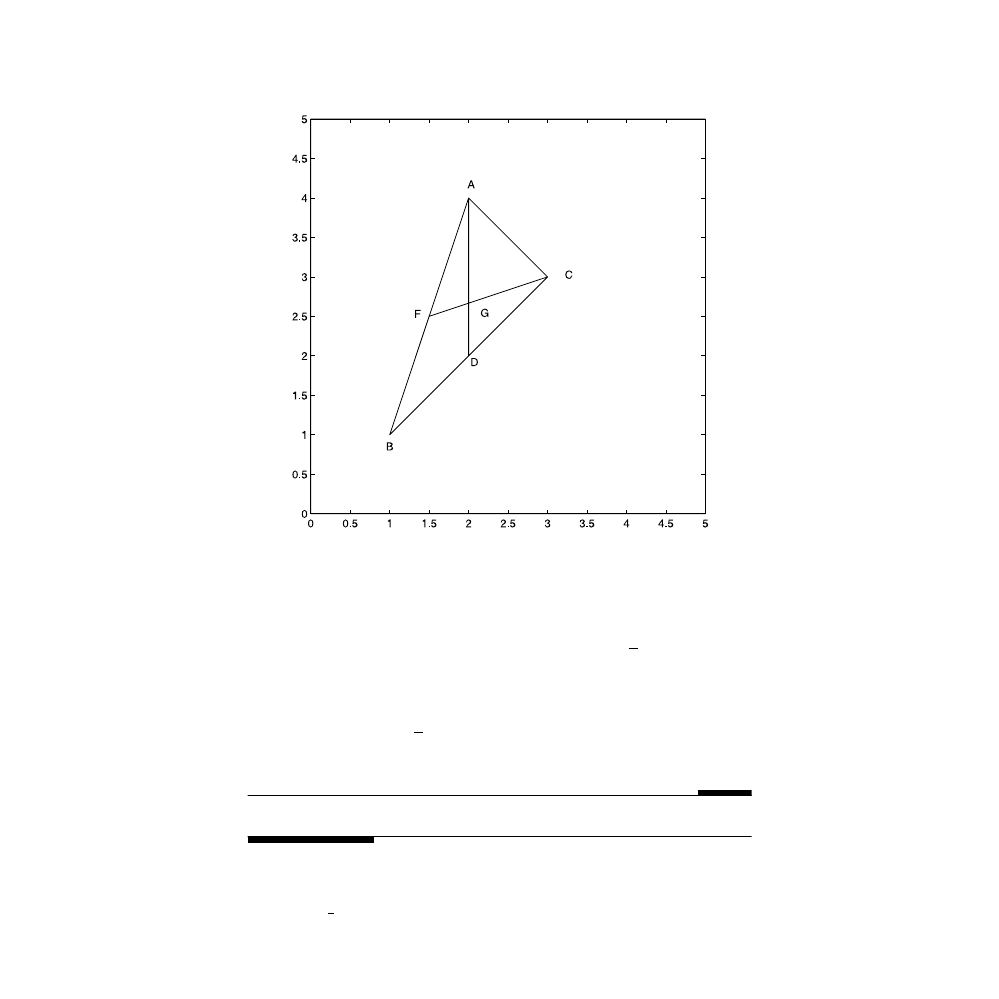
Pb. 6.6
Consider the triangle
∆(ABC), in which D is the midpoint of the BC
segment, and let the point G be defined such that
Assuming
that z
A
, z
B
, z
C
are the complex numbers representing the points (A, B, C):
a.
Find the complex number z
G
that represents the point G.
b.
Show that
and that F is the midpoint of the segment
(AB).
6.3
Complex Conjugation and Division
DEFINITION
The complex conjugate of a complex number z, which is
denoted by , is given by:
FIGURE 6.1
The center of mass of a triangle. (Refer to Pb. 6.6).
(
)
(
).
GD
AD
=
1
3
(
)
(
)
CG
CF
=
2
3
z

© 2001 by CRC Press LLC
(6.7)
That is, is obtained from z by reversing the sign of Im(z). Geometrically, z
and form a pair of symmetric points with respect to the real axis (x-axis) in
the complex plane.
In MATLAB, complex conjugation is written as conj(z).
DEFINITION
The modulus of a complex number z = a + jb, denoted by
, is
given by:
(6.8)
Geometrically, it represents the distance between the origin and the point
representing the complex number z in the complex plane, which by
Pythagorean theorem is given by the same quantity.
In MATLAB, the modulus of z is denoted by abs(z).
THEOREM
For any complex number z, we have the result that:
(6.9)
PROOF
Using the above two definitions for the complex conjugate and the
norm, we can write:
In-Class Exercise
Solve the problem analytically, and then use MATLAB to verify your
answers.
Pb. 6.7
Let z = 3 + 4j. Find
Verify the above theorem.
6.3.1
Division
Using the above definitions and theorem, we now want to define the inverse
of a complex number with respect to the multiplication operation. We write
the results in standard form.
z
a
jb
z
a
jb
= −
= +
if
z
z
z
z
a
b
=
+
2
2
z
zz
2
=
zz
a
jb a
jb
a
b
z
= −
+
=
+
=
(
)(
)
2
2
2
z z
zz
, ,
.
and

© 2001 by CRC Press LLC
(6.10)
from which we deduce that:
(6.11)
and
(6.12)
To summarize the above results, and to help you build your syntax for the
quantities defined in this section, edit the following script M-file and execute it:
z=3+4*j
zbar=conj(z)
modulz=abs(z)
modul2z=z*conj(z)
invz=1/z
reinvz=real(1/z)
iminvz=imag(1/z)
In-Class Exercises
Pb. 6.8
Analytically and numerically, obtain in the standard form an
expression for each of the following quantities:
Pb. 6.9
For any pair of complex numbers z
1
and z
2
, show that:
z
z
a
jb
a
jb
a
jb
a
jb
a
b
z
z
−
= =
+
−
−
=
−
+
=
1
2
2
2
1
1
(
)
Re
Re( )
[Re( )]
[Im( )]
1
2
2
z
z
z
z
=
+
Im
Im( )
[Re( )]
[Im( )]
1
2
2
z
z
z
z
=
−
+
a.
b
c.
.
3 4
2 5
3
1
3
1 2
2 3
3
2
+
+
+
−
+
−
+
−
+
j
j
j
j
j
j
j
j
j
(
)(
)
z
z
z
z
z
z
z
z
z z
z z
z
z
z
z
z
z
1
2
1
2
1
2
1
2
1
2
1
2
1
2
1
2
+
=
+
−
=
−
=
=
=
( /
)
/

© 2001 by CRC Press LLC
6.4
Polar Form of Complex Numbers
If we use polar coordinates, we can write the real and imaginary parts of a
complex number z = a + jb in terms of the modulus of z and the polar angle
θ:
(6.13)
(6.14)
and the complex number z can then be written in polar form as:
(6.15)
The angle
θ is called the argument of z and is usually evaluated in the interval
–
π ≤ θ ≤ π. However, we still have the same complex number if we added to
the value of
θ an integer multiple of 2π.
(6.16)
From the above results, it is obvious that the argument of the complex con-
jugate of a complex number is equal to minus the argument of this complex
number.
In MATLAB, the convention for arg(z) is angle(z).
In-Class Exercise
Pb. 6.10
Find the modulus and argument for each of the following complex
numbers:
Plot these points. Can you detect any geometrical pattern? Generalize.
The main advantage of writing complex numbers in polar form is that it
makes the multiplication and division operations more transparent, and pro-
vides a simple geometric interpretation to these operations, as shown below.
a
r
z
=
=
cos( )
cos( )
θ
θ
b
r
z
=
=
sin( )
sin( )
θ
θ
z
z
j z
z
j
=
+
=
+
cos( )
sin( )
(cos( )
sin( ))
θ
θ
θ
θ
θ
θ
=
=
arg( )
tan( )
z
b
a
z
j
z
j
z
j
z
j
z
j
1
2
3
4
5
1 2
2
1 2
1 2
1 2
= +
= +
= −
= − +
= − −
;
;
;
;

© 2001 by CRC Press LLC
6.4.1
New Insights into Multiplication and Division of Complex Numbers
Consider the two complex numbers z
1
and z
2
written in polar form:
(6.17)
(6.18)
Their product z
1
z
2
is given by:
(6.19)
But using the trigonometric identities for the sine and cosine of the sum of
two angles:
(6.20)
(6.21)
the product of two complex numbers can then be written in the simpler form:
(6.22)
That is, when multiplying two complex numbers, the modulus of the product
is the product of the moduli, while the argument is the sum of arguments:
(6.23)
(6.24)
The above result can be generalized to the product of n complex numbers
and the result is:
(6.25)
(6.26)
A particular form of this expression is the De Moivre theorem, which states
that:
z
z
j
1
1
1
1
=
+
(cos( )
sin( ))
θ
θ
z
z
j
2
2
2
2
=
+
(cos( )
sin( ))
θ
θ
z z
z z
j
1 2
1
2
1
2
1
2
1
2
1
2
=
−
+
+
(cos( ) cos( ) sin( ) sin( ))
(sin( ) cos( ) cos( ) sin( ))
θ
θ
θ
θ
θ
θ
θ
θ
cos(
)
cos( ) cos( ) sin( ) sin( )
θ
θ
θ
θ
θ
θ
1
2
1
2
1
2
+
=
−
sin(
)
sin( ) cos( ) cos( ) sin( )
θ
θ
θ
θ
θ
θ
1
2
1
2
1
2
+
=
+
z z
z z
j
1 2
1
2
1
2
1
2
=
+
+
+
[cos(
)
sin(
)]
θ
θ
θ
θ
z z
z z
1 2
1
2
=
arg(
)
arg( ) arg( )
z z
z
z
1 2
1
2
=
+
z z
z
z z
z
n
n
1 2
1
2
…
=
…
arg(
)
arg( ) arg( )
( )
z z
z
z
z
z
n
n
1 2
1
2
…
=
+
+…+

© 2001 by CRC Press LLC
(6.27)
The above results suggest that the polar form of a complex number may be
written as a function of an exponential function because of the additivity of
the arguments upon multiplication. We revisit this issue later.
In-Class Exercises
Pb. 6.11
Show that
.
Pb. 6.12
Explain, using the above results, why multiplication of any com-
plex number by j is equivalent to a rotation of the point representing this
number in the complex plane by
π/2.
Pb. 6.13
By what angle must we rotate the point P(3, 4) to transform it to the
point P
′(4, 3)?
Pb. 6.14
The points z
1
= 1 + 2j and z
2
= 2 + j are adjacent vertices of a regular
hexagon. Find the vertex z
3
that is also a vertex of the same hexagon and that
is adjacent to z
2
(z
3
≠ z
1
).
Pb. 6.15
Show that the points A, B, C representing the complex numbers z
A
,
z
B
, z
C
in the complex plane lie on the same straight line if and only if:
Pb. 6.16
Determine the coordinates of the P
′ point obtained from the point
P(2, 4) through a reflection around the line
Pb. 6.17
Consider two points A and B representing, in the complex plane,
the complex numbers z
1
and
Let P be any point on the circle of radius
1 and centered at the origin (the unit circle). Show that the ratio of the length
of the line segments PA and PB is the same, regardless of the position of point
P on the unit circle.
Pb. 6.18
Find the polar form of each of the following quantities:
(cos( )
sin( ))
cos(
)
sin(
)
θ
θ
θ
θ
+
=
+
j
n
j
n
n
z
z
z
z
j
1
2
1
2
1
2
1
2
=
−
+
−
[cos(
)
sin(
)]
θ
θ
θ
θ
z
z
z
z
A
c
B
c
−
−
is real.
y
x
= +
2
2.
1
1
/ .
z
(
)
(
)
,
(
)(
), (
)
1
1
1
2
1
15
9
2
3 99
+
−
− +
+
+ + +
j
j
j j
j
j
j

© 2001 by CRC Press LLC
6.4.2
Roots of Complex Numbers
Given the value of the complex number z, we are interested here in finding
the solutions of the equation:
v
n
= z
(6.28)
Let us write both the solutions and z in polar forms,
(6.29)
(6.30)
From the De Moivre theorem, the expression for v
n
= z can be written as:
(6.31)
Comparing the moduli of both sides, we deduce by inspection that:
(6.32)
The treatment of the argument should be done with great care. Recalling
that two angles have the same cosine and sine if they are equal or differ from
each other by an integer multiple of 2
π, we can then deduce that:
(6.33)
Therefore, the general expression for the roots is:
(6.34)
Note that the roots reproduce themselves outside the range: k = 0, 1, 2, …,
(n – 1).
In-Class Exercises
Pb. 6.19
Calculate the roots of the equation z
5
– 32 = 0, and plot them in the
complex plane.
v
j
=
+
ρ
α
α
(cos( )
sin( ))
z
r
j
=
+
(cos( )
sin( ))
θ
θ
ρ
α
α
θ
θ
n
n
j
n
r
j
(cos(
)
sin(
))
(cos( )
sin( ))
+
=
+
ρ = r
n
n
k
k
α θ
π
= +
= ± ± ± …
2
0
1
2
3
,
,
,
,
z
r
n
k
n
j
n
k
n
k
n
n
n
1
1
2
2
0 1 2
1
/
/
cos
sin
, , ,
, (
)
=
+
+
+
=
…
−
θ
π
θ
π
with

© 2001 by CRC Press LLC
a.
What geometric shape does the polygon with the solutions as ver-
tices form?
b.
What is the sum of these roots? (Derive your answer both algebra-
ically and geometrically.)
6.4.3
The Function y = e
j
θθθθ
As alluded to previously, the expression cos(
θ) + j sin(θ) behaves very much
as if it was an exponential; because of the additivity of the arguments of each
term in the argument of the product, we denote this quantity by:
e
j
θ
= cos(
θ) + j sin(θ)
(6.35)
PROOF
Compute the Taylor expansion for both sides of the above equation.
The series expansion for e
j
θ
is obtained by evaluating Taylor’s formula at x =
j
θ, giving (see appendix):
(6.36)
When this series expansion for e
j
θ
is written in terms of its even part and odd
part, we have the result:
(6.37)
However, since j
2
= –1, this last equation can also be written as:
(6.38)
which, by inspection, can be verified to be the sum of the Taylor expansions
for the cosine and sine functions.
In this notation, the product of two complex numbers
It is then a simple matter to show that:
If:
(6.39)
Then:
(6.40)
e
n
j
j
n
n
θ
θ
=
=
∞
∑
1
0
!
( )
e
m
j
m
j
j
m
m
m
m
θ
θ
θ
=
+
+
=
∞
=
∞
+
∑
∑
1
2
1
2
1
0
2
0
2
1
(
)!
( )
(
)!
( )
e
m
j
m
j
m
m
m
m
m
m
θ
θ
θ
=
−
+
−
+
=
∞
=
∞
+
∑
∑
(
)
(
)!
( )
(
)
(
)!
( )
1
2
1
2
1
0
2
0
2
1
z
z
r r e
j
1
2
1 2
1
2
and is:
(
)
.
θ θ
+
z
r
j
= exp( )
θ
z
r
j
=
−
exp(
)
θ

© 2001 by CRC Press LLC
and
(6.41)
from which we can deduce Euler’s equations:
(6.42)
and
(6.43)
Example 6.3
Use MATLAB to generate the graph of the unit circle in the complex plane.
Solution:
Because all points on the unit circle are equidistant from the origin
and their distance to the origin (their modulus) is equal to 1, we can generate
the circle by plotting the N-roots of unity, taking a very large value for N. This
can be implemented by executing the following script M-file.
N=720;
z=exp(j*2*pi*[1:N]./N);
plot(z)
axis square
In-Class Exercises
Pb. 6.20
Using the exponential form of the n-roots of unity, and the expres-
sion for the sum of a geometric series (given in the appendix), show that the
sum of these roots is zero.
Pb. 6.21
Compute the following sums:
a.
1 + cos(x) + cos(2x) + … + cos(nx)
b.
sin(x) + sin(2x) + … + sin(nx)
c.
cos(
α) + cos(α + β) + … + cos(α + nβ)
d.
sin(
α) + sin(α + β) + … + sin(α + nβ)
Pb. 6.22
Verify numerically that for z = x + jy:
z
r
j
−
=
−
1
1
exp(
)
θ
cos( )
exp( ) exp(
)
θ
θ
θ
=
+
−
j
j
2
sin( )
exp( ) exp(
)
θ
θ
θ
=
−
−
j
j
j
2

© 2001 by CRC Press LLC
For what values of y is this quantity pure imaginary?
Homework Problems
Pb. 6.23
Plot the curves determined by the following parametric represen-
tations:
a.
z = 1 – jt
0
≤ t ≤ 2
b.
z = t + jt
2
–
∞ < t < ∞
c.
z = 2(cos(t) + j sin(t))
d.
z = 3(t + j – j exp(–jt))
0 < t <
∞
Pb. 6.24
Find the expression y = f(x) and plot the families of curves defined
by each of the corresponding equations:
a.
b.
c.
d.
e.
f.
g.
h.
Pb. 6.25
Find the image of the line Re(z) = 1 upon the transformation z
′ = z
2
+ z. (First obtain the result analytically, and then verify it graphically.)
Pb. 6.26
Consider the following bilinear transformation:
Show how with proper choices of the constants a, b, c, d, we can generate all
transformations of planar geometry (i.e., scaling, rotation, translation, and
inversion).
Pb. 6.27
Plot the curves C
′ generated by the points P′ that are the images of
points on the circle centered at (3, 4) and of radius 5 under the transformation
of the preceding problem, with the following parameters:
Case 1: a = exp(j
π/4), b = 0, c = 0, d = 1
Case 2: a = 1, b = 3, c = 0, d = 1
Case 3: a = 0, b = 1, c = 1, d = 0
lim
exp( )(cos( )
sin( ))
n
n
z
n
x
y
j
y
→∞
+
=
+
1
π
π
2
3
2
< <
t
Re
1
2
z
=
Im
1
2
z
=
Re( )
z
2
4
=
Im( )
z
2
4
=
z
z
−
+
=
3
3
5
arg
z
z
−
+
=
3
3
4
π
z
2
1
3
− =
z
z
=
+
Im( ) 4
′ =
+
+
z
az b
cz d

© 2001 by CRC Press LLC
6.5
Analytical Solutions of Constant Coefficients ODE
Finding the solutions of an ODE with constant coefficients is conceptually
very similar to solving the linear difference equation with constant coeffi-
cients. We repeat the exercise here for its pedagogical benefits and to bring
out some of the finer technical details peculiar to the ODEs of particular inter-
est for later discussions.
The linear differential equation of interest is given by:
(6.44)
In this section, we find the solutions of this ODE for the cases that u(t) = 0 and
u(t) = A cos(
ωt).
The solutions for the first case are referred to as the homogeneous solu-
tions. By substitution, it is a trivial matter to verify that if y
1
(t) and y
2
(t) are
solutions, then c
1
y
1
(t) + c
2
y
2
(t), where c
1
and c
2
are constants, is also a solution.
This is, as previously mentioned, referred to as the superposition principle
for linear systems.
If u(t)
≠ 0, the general solution of the ODE will be the sum of the corre-
sponding homogeneous solution and the particular solution peculiar to the
specific details of u(t). Furthermore, by inspection, it is clear that if the source
can be decomposed into many components, then the particular solution can
be written as the sum of the particular solutions for the different components
and with the same weights as in the source. This property characterizes a lin-
ear system.
DEFINITION
A system L is considered linear if:
(6.45)
where the c’s are constants and the u’s are time-dependent source signals.
6.5.1
Transient Solutions
To obtain the homogeneous solutions, we set u(t) = 0. We guess that the solu-
tion to this homogeneous differential equation is y = exp(st). You may won-
der why we made this guess; the secret is in the property of the exponential
function, whose derivative is proportional to the function itself. That is:
(6.46)
a
d y
dt
a
d
y
dt
a
dy
dt
a y
u t
n
n
n
n
n
n
+
+…+
+
=
−
−
−
1
1
1
1
0
( )
L c u t
c u t
c u t
c L u t
c L u t
c L u t
n n
n
n
(
( )
( )
( ))
( ( ))
( ( ))
( ( ))
1 1
2 2
1
1
2
2
+
+…+
=
+
+…+
d
st
dt
s
st
(exp( ))
exp( )
=

© 2001 by CRC Press LLC
Through this substitution, the above ODE reduces to an algebraic equation,
and the solution of this algebraic equation then reduces to finding the roots
of the polynomial:
(6.47)
We learned in Chapter 5 the MATLAB command for finding these roots,
when needed. Now, using the superposition principle, and assuming all the
roots are distinct, the general solution of the homogeneous differential equa-
tion is given by:
(6.48)
where s
1
, s
2
, …, s
n
are the above roots and c
1
, c
2
, …, c
n
are constant determined
from the initial conditions of the solution and all its derivatives to order n – 1.
NOTE
In the case that two or more of the roots are equal, it is easy to verify
that the solution of the homogeneous ODE includes, instead of a constant
multiplied by the exponential term corresponding to that root, a polynomial
multiplying the exponential function. The degree of this polynomial is (m – 1)
if m is the degeneracy of the root in question.
Example 6.4
Find the transient solutions to the second-order differential equation.
(6.49)
Solution:
The characteristic polynomial associated with this ODE is the sec-
ond-degree equation given by:
(6.50)
The roots of this equation are
The nature of the solutions is very dependent on the sign of the descriminant
(b
2
– 4ac):
• If b
2
– 4ac > 0, the two roots are distinct and real. Call these roots
α
1
and
α
2
; the solution is then:
(6.51)
a s
a
s
a s a
n
n
n
n
+
+…+
+
=
−
−
1
1
1
0
0
y
c
s t
c
s t
c
s t
n
n
homog.
=
+
+…+
1
1
2
2
exp(
)
exp(
)
exp(
)
a
d y
dt
b
dy
dt
cy
2
2
0
+
+
=
as
bs c
2
0
+ + =
s
b
b
ac
a
±
= − ±
−
2
4
2
y
c
t
c
t
homog.
exp(
)
exp(
)
=
+
1
1
2
2
α
α

© 2001 by CRC Press LLC
In many physical problems of interest, we desire solutions that are zero at
infinity, that is, decay over a finite time. This requires that both
α
1
and
α
2
be
negative; or if only one of them is negative, that the c coefficient of the expo-
nentially increasing solution be zero. This class of solutions is called the over-
damped class.
• If b
2
– 4ac = 0, the two roots are equal, and we call this root
α
degen.
.
The solution to the differential equation is
(6.52)
The polynomial, multiplying the exponential function, is of degree one here
because the degeneracy of the root is of degree two. This class of solutions is
referred to as the critically damped class.
• If b
2
– 4ac < 0, the two roots are complex conjugates of each other,
and their real part is negative for physically interesting cases. If we
denote these roots by s
±
= –
α ± jβ, the solutions to the homogeneous
differential equations take the form:
y
homog.
= exp(–
αt)(c
1
cos(
βt) + c
2
sin(
βt))
(6.53)
This class of solutions is referred to as the under-damped class.
In-Class Exercises
Find and plot the transient solutions to the following homogeneous equa-
tions, using the indicated initial conditions:
Pb. 6.28
a = 1, b = 3, c = 2 y(t = 0) = 1 y
′(t = 0) = –3/2
Pb. 6.29
a = 1, b = 2, c = 1 y(t = 0) = 1 y
′(t = 0) = 2
Pb. 6.30
a = 1, b = 5, c = 6 y(t = 0) = 1 y
′(t = 0) = 0
6.5.2
Steady-State Solutions
In this subsection, we find the particular solutions of the ODEs when the
driving force is a single-term sinusoidal.
As pointed out previously, because of the superposition principle, it is also
possible to write the steady-state solution for any combination of such inputs.
This, combined with the Fourier series techniques (briefly discussed in Chap-
ter 7), will also allow you to write the solution for any periodic function.
y
c
c t
t
homog.
degen.
(
) exp(
)
=
+
1
2
α

© 2001 by CRC Press LLC
We discuss in detail the particular solution for the first-order and the sec-
ond-order differential equations because these represent, as previously
shown in Section 4.7, important cases in circuit analysis.
Example 6.5
Find the particular solution to the first-order differential equation:
(6.54)
Solution:
We guess that the particular solution of this ODE is a sinusoidal of
the form:
(6.55)
Our task now is to find B
c
and B
s
that would force Eq. (6.55) to be the solution
of Eq. (6.54). Therefore, we substitute this trial solution in the differential
equation and require that, separately, the coefficients of sin(
ωt) and cos(ωt)
terms match on both sides of the resulting equation. These requirements are
necessary for the trial solution to be valid at all times. The resulting condi-
tions are
(6.56)
from which we can also deduce the polar form of the solution, giving:
(6.57)
Example 6.6
Find the particular solution to the second-order differential equation:
(6.58)
Solution:
Again, take the trial particular solution to be of the form:
a
dy
dt
by
A
t
+
= cos( )
ω
y
t
B
t
B
t
t
B
t
B
t
c
s
partic.
( )
cos(
)
[cos( ) cos(
) sin( ) sin(
)]
cos(
)
sin(
)
=
−
=
+
=
+
ω
φ
φ
ω
φ
ω
ω
ω
B
a
b
B
B
Ab
a
b
s
c
c
=
=
+
ω
ω
2
2
2
B
A
a
b
a
b
2
2
2
2
2
=
+
=
ω
φ
ω
tan( )
a
d y
dt
b
dy
dt
cy
A
t
2
2
+
+
= cos( )
ω

© 2001 by CRC Press LLC
(6.59)
Repeating the same steps as in Example 6.5, we find:
(6.60)
(6.61)
6.5.3
Applications to Circuit Analysis
An important application of the above forms for the particular solutions is in
circuit analysis with inductors, resistors, and capacitors as elements. We
describe later a more efficient analytical method (phasor representation) for
solving this kind of problem; however, we believe that it is important that
you also become familiar with the present technique.
6.5.3.1
RC Circuit
Referring to the RC circuit shown in
, we derived the differential
equation that the potential difference across the capacitor must satisfy;
namely:
(6.62)
This is a first-order differential equation, the particular solution of which is
given in Example 6.5 if we were to identify the coefficients in the ODE as fol-
lows: a = RC, b = 1, A = V
0
.
6.5.3.2
RLC Circuit
Referring to the circuit, shown in
, the voltage across the capacitor
satisfies the following ODE:
(6.63)
This equation can be identified with that given in Example 6.6 if the ODE
coefficients are specified as follows: a = LC, b = RC, c = 1, A = V
0
.
y
t
B
t
B
t
t
B
t
B
t
c
s
partic.
( )
cos(
)
[cos( ) cos(
) sin( ) sin(
)]
cos(
)
sin(
)
=
−
=
+
=
+
ω
φ
φ
ω
φ
ω
ω
ω
B
b
c a
b
A
B
c a
c a
b
A
s
c
=
−
+
=
−
−
+
ω
ω
ω
ω
ω
ω
(
)
(
)
(
)
2 2
2 2
2
2 2
2 2
B
A
c a
b
b
c a
2
2
2 2
2 2
2
=
−
+
=
−
(
)
tan( )
ω
ω
φ
ω
ω
RC
dV
dt
V
V
t
C
C
+
=
0
cos(
)
ω
LC
d V
dt
RC
dV
dt
V
V
t
c
C
C
2
2
0
+
+
=
cos(
)
ω

© 2001 by CRC Press LLC
In-Class Exercises
Pb. 6.31
This problem pertains to the RC circuit:
a.
Write the output signal V
C
in the amplitude-phase representation.
b.
Plot the gain response as a function of a normalized frequency that
you will have to select. (The gain of a circuit is defined as the ratio
of the amplitude of the output signal over the amplitude of the
input signal.)
c.
Determine the phase response of the system (i.e., the relative phase
of the output signal to that of the input signal as function of the
frequency) also as function of the normalized frequency.
d.
Can this circuit be used as a filter (i.e., a device that lets through only
a specified frequency band)? Specify the parameters of this band.
Pb. 6.32
This problem pertains to the RLC circuit:
a.
Write the output signal V
C
in the amplitude-phase representation.
b.
Defining the resonance frequency of this circuit as:
find
at which frequency the gain is maximum, and find the width of
the gain curve.
c.
Plot the gain curve and the phase curve for the following cases:
.
d.
Can you think of a possible application for this circuit?
Pb. 6.33
Can you think of a mechanical analog to the RLC circuit? Identify
in that case the physical parameters in the corresponding ODE.
Pb. 6.34
Assume that the source potential in the RLC circuit has five fre-
quency components at
ω, 2ω, …, 5ω of equal amplitude. Plot the input and
output potentials as a function of time over the interval 0 <
ωt < 2π. Assume
that
6.6
Phasors
A technique in widespread use to compute the steady-state solutions of sys-
tems with sinusoidal input is the method of phasors. In this and the following
two chapter sections, we define phasors, learn how to use them to add two or
ω
0
1
=
LC
,
ω
0
L
R
= 0.1, 1, 10
ω ω
ω
=
=
=
0
0
1
1
LC
L
R
and
.

© 2001 by CRC Press LLC
more signals having the same frequency, and how to find the particular solu-
tion of an ODE with a sinusoidal driving function.
There are two key ideas behind the phasor representation of a signal:
1. A real, sinusoidal time-varying signal may be represented by a
complex time-varying signal.
2. This complex signal can be represented as the product of a complex
number that is independent of time and a complex signal that is
dependent on time.
Example 6.7
Decompose the signal V = A cos(
ωt + φ) according to the above prescription.
Solution:
This signal can, using the polar representation of complex num-
bers, also be written as:
(6.64)
where the phasor, denoted with a tilde on top of its corresponding signal
symbol, is given by:
(6.65)
(Warning: Do not mix the tilde symbol that we use here, to indicate a phasor,
with the overbar that denotes complex conjugation.)
Having achieved the above goal of separating the time-independent part of
the complex number from its time-dependent part, we now learn how to
manipulate these objects. A lot of insight can be immediately gained if we
note that this form of the phasor is exactly in the polar form of a complex
number, with clear geometric interpretation for its magnitude and phase.
6.6.1
Phasor of Two Added Signals
The sum of two signals with common frequencies but different amplitudes
and phases is
(6.66)
To write the above result in phasor notation, note that the above sum can also
be written as follows:
(6.67)
V
A
t
A
j
t
Ae e
j
j t
=
+
=
+
=
cos(
)
Re[ exp( (
))] Re[
]
ω
φ
ω
φ
φ
ω
˜
V
Ae
j
=
φ
V
A
t
A
t
A
t
tot
tot
tot
.
.
.
cos(
)
cos(
)
cos(
)
=
+
=
+
+
+
ω
φ
ω
φ
ω
φ
1
1
2
2
V
A
j
t
A
j
t
A e
A e
e
tot
j
j
j t
.
Re[
exp( (
))
exp( (
))]
Re[(
)
]
=
+
+
+
=
+
1
1
2
2
1
2
1
2
ω
φ
ω
φ
φ
φ
ω

© 2001 by CRC Press LLC
and where
(6.68)
Preparatory Exercise
Pb. 6.35
Write the analytical expression for A
tot.
and
φ
tot.
in Eq. (6.68) as func-
tions of the amplitudes and phases of signals 1 and 2.
The above result can, of course, be generalized to the sum of many signals;
specifically:
(6.69)
and
(6.70)
(6.71)
(6.72)
That is, the resultant field can be obtained through the simple operation of
adding all the complex numbers (phasors) that represent each of the individ-
ual signals.
Example 6.8
Given ten signals, the phasor of each of the form
where the ampli-
tude and phase for each have the functional forms
write
a MATLAB program to compute the resultant sum phasor.
˜
˜
˜
.
.
.
V
A e
V
V
tot
tot
j
tot
=
=
+
φ
1
2
V
A
t
A
t
A
j t
j
e
A e
tot
tot
tot
n
n
n
N
n
n
n
N
j t
n
j
n
N
n
.
.
.
cos(
)
cos(
)
Re
exp(
)
Re
=
+
=
+
=
+
=
=
=
=
∑
∑
∑
ω
φ
ω
φ
ω
φ
ω
φ
1
1
1
˜
˜
.
V
V
tot
n
n
N
=
=
∑
1
⇒
=
A
V
tot
tot
.
.
˜
φ
tot
tot
V
.
.
arg( ˜ )
=
A e
n
j
n
φ
,
A
n
n
n
n
=
=
1
2
and
φ
,

© 2001 by CRC Press LLC
Solution:
Edit and execute the following script M-file:
N=10;
n=1:N;
amplituden=1./n;
phasen=n.^2;
phasorn=amplituden.*exp(j.*phasen);
phasortot=sum(phasorn);
amplitudetot=abs(phasortot)
phasetot=angle(phasortot)
In-Class Exercises
Pb. 6.36
Could you have estimated the answer to Example 6.8? Justify your
reasoning.
Pb. 6.37
Show that if you add N signals with the same magnitude and fre-
quency but with phases equally distributed over the [0, 2
π] interval, the
resultant phasor will be zero. (Hint: Remember the result for the sum of the
roots of unity.)
Pb. 6.38
Show that the resultant signal from adding N signals having the
same frequency has the largest amplitude when all the individual signals are
in phase (this situation is referred to as maximal constructive interference).
Pb. 6.39
In this problem, we consider what happens if the frequency and
amplitude of N different signals are still equal, but the different phases of the
signals are randomly distributed over the [0, 2
π] interval. Find the amplitude
of the resultant signal if N = 1000, and compare it with the maximal construc-
tive interference result. (Hint: Recall that the rand(1,N) command gener-
ates a 1-D array of N random numbers from the interval [0, 1].)
Pb. 6.40
The service provided to your home by the electric utility company
is a two-phase service. This means that two 110-V/60-Hz hot lines plus a neu-
tral (ground) line terminate in your panel. The hot lines are
π out of phase.
a.
Which signal would you use to drive your clock radio or your
toaster?
b.
What configuration will you use to drive your oven or your dryer?
Pb. 6.41
In most industrial environments, electric power is delivered in
what is called a three-phase service. This consists of three 110-V/60-Hz lines
with phases given by (0, 2
π/3, 4π/3). What is the maximum voltage that you
can obtain from any combination of two of these signals?
Pb. 6.42
Two- and three-phase power can be extended to N-phase power. In
such a scheme, the N-110-V/60-Hz signals are given by:

© 2001 by CRC Press LLC
While the sum of the voltage of all the lines is zero, the instantaneous power
is not. Find the total power, assuming that the power from each line is pro-
portional to the square of its time-dependent expression. (Hint: Use the dou-
ble angle formula for the cosine function.)
NOTE
Another designation in use for a 110-V line is an rms value of 110, and
not the value of the maximum amplitude as used above.
6.7
Interference and Diffraction of Electromagnetic Waves
6.7.1
The Electromagnetic Wave
Electromagnetic waves (em waves) are manifest as radio and TV broadcast
signals, microwave communication signals, light of any color, X-rays,
γ-rays,
etc. While these waves have different sources and methods of generation and
require different kinds of detectors, they do share some general characteris-
tics. They differ from each other only in the value of their frequencies. Indeed,
it was one of the greatest intellectual achievements of the 19th century when
Maxwell developed the system of equations, now named in his honor, to
describe these waves’ commonality. The most important of these properties
is that they all travel in a vacuum with, what is called, the speed of light c (c
= 3
× 10
8
m/s). The detailed study of these waves is the subject of many elec-
trophysics subspecialties.
Electromagnetic waves are traveling waves. To understand their mathe-
matical nature, consider a typical expression for the electric field associated
with such waves:
E(z, t) = E
0
cos[kz –
ωt]
(6.73)
Here, E
0
is the amplitude of the wave, z is the spatial coordinate parallel to
the direction of propagation of the wave, and k is the wavenumber.
V
t
n
N
n
N
n
=
+
=
…
−
110
120
2
0 1
1
cos
, ,
,
π
and
p t
A
t
n
N
P
p
n
n
n
N
( )
cos
=
+
=
=
−
∑
2
2
0
1
2
ω
π
and

© 2001 by CRC Press LLC
Note that if we plot the field for a fixed time, for example, at t = 0, the field
takes the shape of a sinusoidal function in space:
E(z, t = 0) = E
0
cos[kz]
(6.74)
From the above equation, one deduces that the wavenumber k = 2
π/λ, where
λ is the wavelength of the wave (i.e., the length after which the wave shape
reproduces itself).
Now let us look at the field when an observer, located at z = 0, would mea-
sure it as a function of time. Then:
E(z = 0, t) = E
0
cos[
ωt]
(6.75)
The temporal period, that is, the time after which the wave shape reproduces
itself, is
where
ω is the angular frequency of the wave.
Next, we want to relate the wavenumber to the angular frequency. To do
that, consider an observer located at z = 0. The observer measures the field at
t = 0 to be E
0
. At time
∆t later, he should measure the same field, whether he
uses Eq. (6.74) or (6.75) if he takes
∆z = c∆t, the distance that the wave crest
has moved, and where c is the speed of propagation of the wave. From this,
one deduces that the wavenumber and the angular frequency are related by
kc =
ω. This relation holds true for all electromagnetic waves; that is, as the
frequency increases, the wavelength decreases.
If two traveling waves have the same amplitude and frequency, but one is
traveling to the right while the other is traveling to the left, the result is a
standing wave. The following program permits visualization of this standing
wave.
x=0:0.01:5;
a=1;
k=2*pi;
w=2*pi;
t=0:0.05:2;
M=moviein(41);
for m=1:41;
z1=cos(k*x-w*t(m));
z2=cos(k*x+w*t(m));
z=z1+z2;
plot(x,z,'r');
axis([0 5 -3 3]);
T
=
2
π
ω
,

© 2001 by CRC Press LLC
M(:,m)=getframe;
end
movie(M,20)
Compare the spatio-temporal profile of the resultant to that for a single wave
(i.e., set x2 = 0).
6.7.2
Addition of Two Electromagnetic Waves
In many practical instances, we are faced with the problem that two em
waves originating from the same source, but following different spatial
paths, meet again at a certain position. We want to find the total field at this
position resulting from adding the two waves. We first note that, in the sim-
plest case where the amplitude of the two fields are kept equal, the effect of
the different paths is only to dephase one of the waves from the other by an
amount:
∆φ = k∆l, where ∆l is the path difference. In effect, the total field is
given by:
(6.76)
where
∆φ = φ
1
–
φ
2
. This form is similar to those studied in the addition of two
phasors and we will hence describe the problem in this language.
The resultant phasor is
(6.77)
Preparatory Exercise
Pb. 6.43
Find the modulus and the argument of the resultant phasor given
in Eq. (6.74) as a function of E
0
and
∆φ. From this expression, deduce the rela-
tion that relates the path difference corresponding to when the resultant pha-
sor has maximum magnitude and that when its magnitude is a minimum.
The curve describing the modulus square of the resultant phasor is what is
commonly referred to as the interference pattern of two waves.
6.7.3
Generalization to N-waves
The addition of electromagnetic waves can be generalized to N-waves.
E
t
E
t
E
t
tot.
( )
cos[
]
cos[
]
=
+
+
+
0
1
0
2
ω
φ
ω
φ
˜
˜
˜
.
E
E
E
tot
=
+
1
2

© 2001 by CRC Press LLC
Example 6.9
Find the resultant field of equal-amplitude N-waves, each phase-shifted from
the preceding by the same
∆φ.
Solution:
The problem consists of computing an expression of the following
kind:
(6.78)
We have encountered such an expression previously. This sum is that corre-
sponding to the sum of a geometric series. Computing this sum, the modulus
square of the resultant phasor is
(6.79)
Because the source is the same for each of the components, the modulus of
each phasor is related to the source amplitude by E
0
= E
source
/N. It is usually
as function of the source field that the results are expressed.
In-Class Exercises
Pb. 6.44
Plot the normalized square modulus of the resultant of N-waves as
a function of
∆φ for different values of N (5, 50, and 500) over the interval –π
<
∆φ < π.
Pb. 6.45
Find the dependence of the central peak value of Eq. (6.79) on N.
Pb. 6.46
Find the phase shift that corresponds to the position of the first
minimum of Eq. (6.79).
Pb. 6.47
Find in Eq. (6.79) the relative height of the first maximum (i.e., the
one following the central maximum) to that of the central maximum as a
function of N.
Pb. 6.48
In an antenna array with the field representing N aligned, equally
spaced individual antennae excited by the same source is given by Eq. (6.78).
If the line connecting the point of observation to the center of the array is
making an angle
θ with the antenna array, the phase shift is
˜
˜
˜
˜
(
)
.
E
E
E
E
E
e
e
e
tot
n
j
j
j N
=
+
+…+
=
+
+
+…+
−
(
)
1
2
0
2
1
1
∆
∆
∆
φ
φ
φ
˜
(
)
(
)
(
)
(
)
cos(
)
cos(
)
sin (
/ )
sin (
/ )
.
E
E
e
e
e
e
E
N
E
N
tot
j N
j
j N
j
2
0
2
0
2
0
2
2
2
1
1
1
1
1
1
2
2
=
−
−
−
−
=
−
−
=
−
−
∆
∆
∆
∆
∆
∆
∆
∆
φ
φ
φ
φ
φ
φ
φ
φ
∆φ
π
λ
θ
=
2
d cos( ),

© 2001 by CRC Press LLC
where
λ is the wavelength of radiation and d is the spacing between two con-
secutive antennae. Draw the polar plot of the total intensity as function of the
angle
θ for a spacing d = λ/2 for different values of N (2, 4, 6, and 10).
Pb. 6.49
Do the results of Pb. 6.48 suggest to you a strategy for designing a
multi-antenna system with sharp directivity? Can you think of a method,
short of moving the antennae around, that permits this array to sweep a
range of angles with maximum directivity?
Pb. 6.50
The following program simulates a 25-element array-swept radar
beam.
th=0:0.01:pi;
t=-0.5*sqrt(3):0.05*sqrt(3):0.5*sqrt(3);
N=25;
M=moviein(21);
for m=1:21;
I=(1/N^2)*(sin(N*((pi/4)*cos(th)+(pi/4)*t(m)))...
^2)./((sin((pi/4)*cos(th)+(pi/4)*t(m))).^2);
polar(th,I);
M(:,m)=getframe;
end
movie(M,10)
a.
Determine the range of the sweeping angle.
b.
Can you think of an electronic method for implementing this task?
6.8
Solving ac Circuits with Phasors: The Impedance Method
In Section 6.5, we examined the conventional technique for solving some sim-
ple ac circuits problems. We suggested that using phasors may speed up the
determination of the solution. This is the subject of this chapter section.
We will treat, using this technique, the simple RLC circuit already solved
through other means in order to give you a measure of the simplifications
that can be achieved in circuit analysis through this technique. We then pro-
ceed to use the phasor technique to investigate another circuit configuration:
the infinite LC ladder. The power of the phasor technique will also be put to
use when we, topologically, solve much more difficult circuit problems than
the one-loop category encountered thus far. Essentially, a straightforward

© 2001 by CRC Press LLC
algebraic technique can give the voltages and currents for any circuit. We
illustrate this latter case in Chapter 8.
Recalling that the voltage drops across resistors, inductors, and capacitors
can all be expressed as function of the current, its derivative, and its integral,
our goal is to find a technique to replace these operators by simple algebraic
operations. The key to achieving this goal is to realize that:
If:
(6.80)
Then:
(6.81)
and
(6.82)
From Eqs. (4.25) to (4.27) and Eqs. (6.80) to (6.82), we can deduce that the pha-
sors representing the voltages across resistors, inductors, and capacitors can
be written as follows:
(6.83)
(6.84)
(6.85)
The terms multiplying the current phasor on the RHS of each of the above
equations are called the resistor, the inductor, and the capacitor impedances,
respectively.
6.8.1
RLC Circuit Phasor Analysis
Let us revisit this problem first discussed in Section 4.7. Using Kirchoff’s volt-
age law and Eqs. (6.83) to (6.85), we can write the following relation between
the phasor of the current and that of the source potential:
(6.86)
I
I
t
e
I e
j t
j
=
+
=
0
0
cos(
)
Re[
(
)]
ω
φ
ω
φ
dI
dt
I
t
e
I j
e
j t
j
= −
+
=
0
0
ω
ω
φ
ω
ω
φ
sin(
)
Re[
( (
)
)]
Idt
I
t
e
I
j
e
j t
j
=
+
=
∫
0
0
1
ω
ω
φ
ω
ω
φ
sin(
)
Re
˜
˜
˜
V
IR
IZ
R
R
=
=
˜
˜
˜
V
I j L
IZ
L
L
=
( )
=
ω
˜
˜
˜
V
I
j C
IZ
C
C
=
( )
=
ω
˜
˜
˜(
)
˜
˜
V
IR I j L
I
j C
I R
j L
j C
s
=
+
+
( )
=
+
+
ω
ω
ω
ω
1

© 2001 by CRC Press LLC
That is, we can immediately compute the modulus and the argument of the
phasor of the current if we know the values of the circuit components, the
source voltage phasor, and the frequency of the source.
In-Class Exercises
Using the expression for the circuit resonance frequency
ω
0
previously intro-
duced in Pb. 6.32, for the RLC circuit:
Pb. 6.51
Show that the system’s total impedance can be written as:
Pb. 6.52
Show that
and from this result, deduce the value
of
ν at which the impedance is entirely real.
Pb. 6.53
Find the magnitude and the phase of the total impedance.
Pb. 6.54
Selecting for the values of the circuit elements LC = 1, RC = 3, and
ω = 1, compare the results that you obtain through the phasor analytical
method with the numerical results for the voltage across the capacitor in an
RLC circuit that you found while solving Eq. (4.36).
The Transfer Function
As you would have discovered solving Pb. 6.54, the ratio of the phasor of the
potential difference across the capacitor with that of the ac source can be
directly calculated once the value of the current phasor is known. This ratio
is called the Transfer Function for this circuit if the voltage across the capaci-
tor is taken as the output of this circuit. It is obtained by combining Eqs. (6.85)
and (6.86) and is given by:
(6.87)
The Transfer Function concept can be generalized to any ac circuit. It refers
to the ratio of the output voltage phasor to the input voltage phasor. It incor-
porates all the relevant information on the details of the circuit. It is the stan-
dard form for representing the response of a circuit to a single sinusoidal
function input.
Z
R
j
L
LC
= +
−
=
=
ω
ν
ν
ν
ω
ω
ω
0
0
1
, where
Z
Z
( )
( / );
ν
ν
=
1
˜
˜
(
)
( )
V
V
j RC
LC
H
c
s
=
−
+
=
1
1
2
ω
ω
ω
© 2001 by CRC Press LLC
Homework Problem
Pb. 6.55
Plot the magnitude and the phase of theTransfer Function given in
Eq. (6.87) as a function of
ω, for LC = 1, RC = 3.
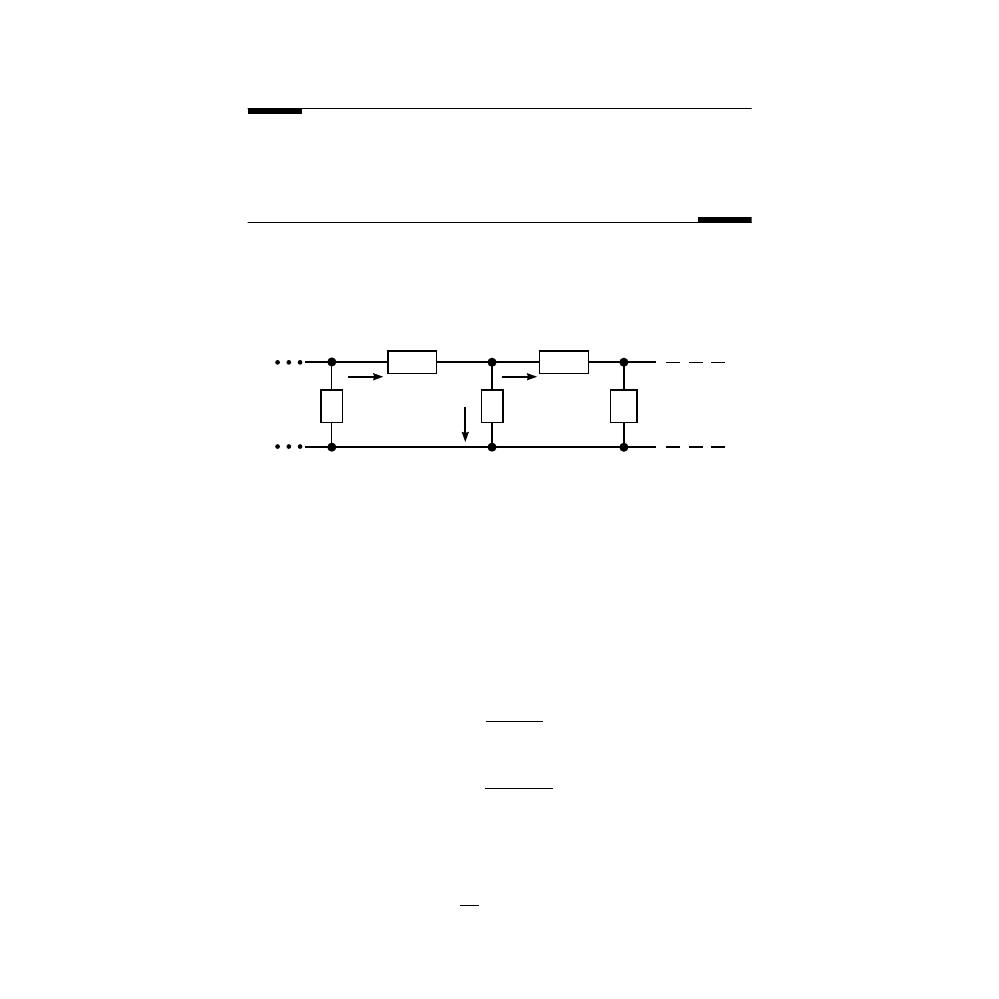
6.8.2
The Infinite LC Ladder
The LC ladder consists of an infinite repetition of the basic elements shown in
Using the definition of impedances, the phasors of the n and (n + 1) voltages
and currents are related through:
(6.88)
(6.89)
From Eq. (6.88), we deduce the following expressions for
(6.90)
(6.91)
Substituting these values for the currents in Eq. (6.89), we deduce a second-
order difference equation for the voltage phasor:
(6.92)
FIGURE 6.2
The circuit of an infinite LC ladder.
V
n
V
n+1
I
n
(I
n –
I
n+1
)
I
n+1
Z
1
Z
2
Z
2
Z
2
Z
1
˜
˜
˜
V
V
Z I
n
n
n
−
=
+1
1
˜
(˜
˜
)
V
I
I
Z
n
n
n
+
+
=
−
1
1
2
˜
˜
:
I
I
n
n
and
+1
˜
˜
˜
I
V
V
Z
n
n
n
=
−
+1
1
˜
˜
˜
I
V
V
Z
n
n
n
+
+
+
=
−
1
1
2
1
˜
˜
˜
V
Z
Z
V
V
n
n
n
+
+
−
+
+
=
2
1
2
1
2
0

© 2001 by CRC Press LLC
The solution of this difference equation can be directly obtained by the
techniques discussed in Chapter 2 for obtaining solutions of homogeneous
difference equations. The physically meaningful solution is given by:
(6.93)
and the voltage phasor at node n is then given by:
(6.94)
We consider the model where Z
1
= j
ωL and Z
2
= 1/(j
ωC), respectively, for an
inductor and a capacitor. The expression for
λ then takes the following form:
(6.95)
where the normalized frequency is defined by
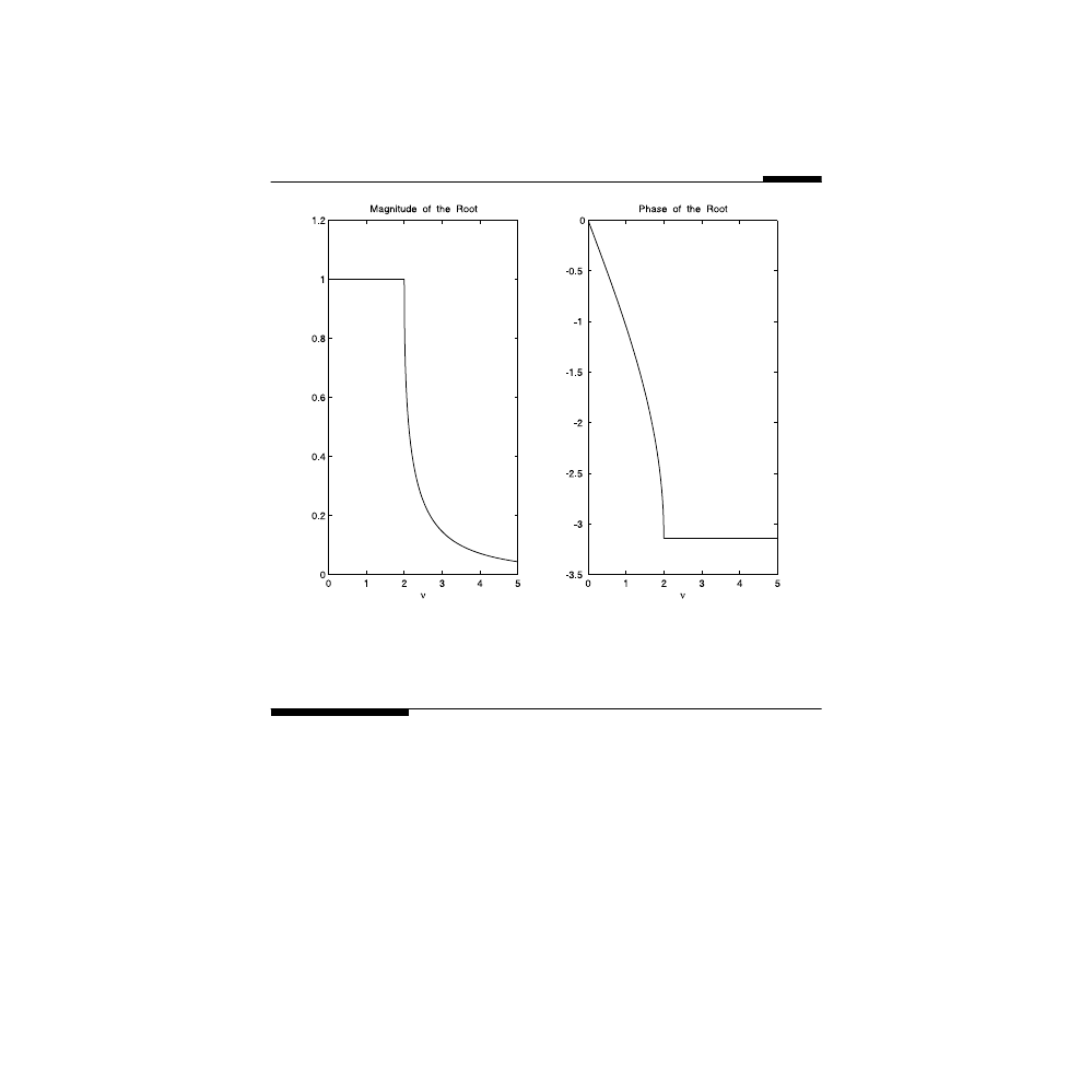
We plot in
the magnitude and the phase of the root
λ as function of the nor-
malized frequency.
As can be directly observed from an examination of
tude of
λ is equal to 1 (i.e., the magnitude of is also 1) for υ < υ
cutoff
= 2, while
it drops precipitously after that, with the dropoff in the potential much
steeper with increasing node number. Physically, this represents extremely
short penetration through the ladder for signals with frequencies larger than
the cutoff frequency. Furthermore, note that for
υ < υ
cutoff
= 2, the phase of
increases linearly with the index n; and because it is negative, it corresponds
to a delay in the signal as it propagates down the ladder, which corresponds
to a finite velocity of propagation for the signal.
Before we leave this ladder circuit, it is worth addressing a practical con-
cern. While it is impossible to realize an infinite-dimensional ladder, the
above conclusions do not change by much if we replace the infinite ladder by
a finite ladder and we terminate it after awhile by a resistor with resistance
equal to
In-Class Exercise
Pb. 6.56
Repeat the analysis given above for the LC ladder circuit, if instead
we were to:
a.
Interchange the positions of the inductors and the capacitors in the
ladder circuit. Based on this result and the above LC result, can
you design a bandpass filter with a flat response?
λ = +
−
+
1
1
2
4
2
1
1
2
2
1
Z
Z
Z
Z Z
˜
˜
V
V
n
s
n
= λ
λ
υ
υ
υ
=
−
−
−
1
2
4
2
2
4
1 2
j
/
υ ω ω
ω
=
=
/
.
0
LC
˜
V
n
˜
V
n
L C
/ .
© 2001 by CRC Press LLC
b.
Interchange the inductor elements by resistors. In particular, com-
pute the input impedance of this circuit.
6.9
Transfer Function for a Difference Equation with
Constant Coefficients*
In Section 6.8.1, we found the Transfer Function for what essentially was a
simple ODE. In this section, we generalize the technique to find the Transfer
Function of a difference equation with constant coefficients. The form of the
difference equation is given by:
(6.96)
Along the same route that we followed in the phasor treatment of ODE,
assume that both the input and output are of the form:
FIGURE 6.3
The magnitude (left panel) and the phase (right panel) of the characteristic root of the infinite
LC ladder.
y k
b u k
b u k
b u k
m
a y k
a y k
a y k n
m
n
( )
( )
(
)
(
)
(
)
(
)
(
)
=
+
− +…+
−
−
− −
− −…−
−
0
1
1
2
1
1
2

© 2001 by CRC Press LLC
(6.97)
where
Ω is a normalized frequency; typically, in electrical engineering appli-
cations, the real frequency multiplied by the sampling time. Replacing these
expressions in the difference equation, we obtain:
(6.98)
where, by convention, z = e
j
Ω
.
Example 6.10
Find the Transfer Function of the following difference equation:
(6.99)
Solution:
By direct substitution into Eq. (6.98), we find:
(6.100)
It is to be noted that the Transfer Function is a ratio of two polynomials. The
zeros of the numerator are called the zeros of the Transfer Function, while the
zeros of the denominator are called its poles. If the coefficients of the differ-
ence equations are real, then by the Fundamental Theorem of Algebra, the
zeros and the poles are either real or are pairs of complex conjugate numbers.
The Transfer Function fully describes any linear system. As will be shown
in linear systems courses, the z-transform of the Transfer Function gives the
weights for the solution of the difference equation, while the values of the
poles of the Transfer Function determine what are called the system modes
of the solution. These are the modes intrinsic to the circuit, and they do not
depend on the specific form of the input function.
Furthermore, it is worth noting that the study of recursive filters, the back-
bone of digital signal processing, can be simply reduced to a study of the
Transfer Function under different configurations. In Applications 2 and 3 that
follow, we briefly illustrate two particular digital filters in wide use.
u k
Ue
y k
Ye
j k
j k
( )
( )
=
=
Ω
Ω
and
Y
U
b e
a e
b z
a z
H z
l
j l
l
m
l
j l
l
n
l
l
l
m
l
l
l
n
=
+
=
+
≡
−
=
−
=
−
=
−
=
∑
∑
∑
∑
Ω
Ω
0
1
0
1
1
1
( )
y k
u k
y k
y k
( )
( )
(
)
(
)
=
+
− −
−
2
3
1
1
3
2
H z
z
z
z
z
z
( )
=
−
+
=
−
+
−
−
1
1
2
3
1
3
2
3
1
3
1
2
2
2

© 2001 by CRC Press LLC
Application 1
Using the Transfer Function formalism, we want to estimate the accuracy of
the three integrating schemes discussed in Chapter 4. We want to compare
the Transfer Function of each of those algorithms to that of the exact result,
obtained upon integrating exactly the function e
j
ωt
.
The exact result for integrating the function e
j
ωt
is, of course,
thus giv-
ing for the exact Transfer Function for integration the expression:
(6.101)
Before proceeding with the computation of the transfer function for the dif-
ferent numerical schemes, let us pause for a moment and consider what we
are actually doing when we numerically integrate a function. We go through
the following steps:
1. We discretize the time interval over which we integrate; that is, we
define the sampling time
∆t, such that the discrete points abscissa
are given by k(
∆t), where k is an integer.
2. We write a difference equation for the integral relating its values
at the discrete points with its values and that of the integrand at
discrete points with equal or smaller indices.
3. We obtain the value of the integral by iterating the defining differ-
ence equation.
The test function used for the estimation of the integration methods accu-
racy is written at the discrete points as:
(6.102)
The difference equations associated with each of the numerical integration
schemes are:
(6.103)
(6.104)
(6.105)
leading to the following expressions for the respective Transfer Functions:
e
j
j t
ω
ω
,
H
j
exact
=
1
ω
y k
e
j k
t
( )
(
)
=
ω ∆
I k
I k
t
y k
y k
T
T
(
)
( )
( (
)
( ))
+ =
+
+ +
1
2
1
∆
I
k
I
k
ty k
MP
MP
(
)
( )
(
/ )
+ =
+
+
1
1 2
∆
I k
I k
t
y k
y k
y k
S
S
(
)
(
)
( (
)
( )
(
))
+ =
− +
+ +
+
−
1
1
3
1
4
1
∆

© 2001 by CRC Press LLC
(6.106)
(6.107)
(6.108)
The measures of accuracy of the integration scheme are the ratios of these
Transfer Functions to that of the exact expression. These are given, respec-
tively, by:
(6.109)
(6.110)
(6.111)
gives the value of this ratio as a function of the number of sam-
pling points, per oscillation period, selected in implementing the different
integration subroutines:
As can be noted, the error is less than 1% for any of the discussed methods as
long as the number of points in one oscillation period is larger than 20,
although the degree of accuracy is best, as we expected based on geometrical
arguments, for Simpson’s rule.
In a particular application, where a finite number of frequencies are simul-
taneously present, the choice of (
∆t) for achieving a specified level of accuracy
TABLE 6.1
Accuracy of the Different Elementary Numerical Integrating Methods
Number of Sampling Points in a Period
R
T
R
MP
R
S
100
0.9997
1.0002
1.0000
50
0.9986
1.0007
1.0000
40
0.9978
1.0011
1.0000
30
0.9961
1.0020
1.0000
20
0.9909
1.0046
1.0001
10
0.9591
1.0206
1.0014
5
0.7854
1.1107
1.0472
H
t e
e
T
j
t
j
t
=
+
−
∆
∆
∆
2
1
1
ω
ω
(
)
(
)
H
t
e
e
MP
j
t
j
t
=
−
∆
∆
∆
ω
ω
(
)/
(
)
2
1
H
t e
e
e
e
S
j
t
j
t
j
t
j
t
=
+ +
−
−
−
∆
∆
∆
∆
∆
3
4
(
)
(
)
(
)
(
)
(
)
ω
ω
ω
ω
R
t
t
t
T
=
(
/ )
sin(
/ )
cos(
/ )
ω
ω
ω
∆
∆
∆
2
2
2
R
t
t
MP
=
(
/ )
sin(
/ )
ω
ω
∆
∆
2
2
R
t
t
t
S
=
+
ω
ω
ω
∆
∆
∆
3
2
cos(
)
sin(
)

© 2001 by CRC Press LLC
in the integration subroutine should ideally be determined using the shortest
of the periods present in the integrand.
Application 2
As mentioned earlier, the Transfer Function technique is the prime tool for
the analysis and design of digital filters. In this and the following application,
we illustrate its use in the design of a low-pass digital filter and a digital pro-
totype bandpass filter.
The low-pass filter, as its name indicates, filters out the high-frequency
components from a signal.
Its defining difference equation is given by:
(6.112)
giving for its Transfer Function the expression:
(6.113)
Written as a function of the normalized frequency, it is given by:
(6.114)
We plot, in
, the magnitude and the phase of the transfer function
as a function of the normalized frequency for the value of a = 0.1. Note that
the gain is equal to 1 for
Ω = 0, and decreases monotonically thereafter.
To appreciate the operation of this filter, consider a sinusoidal signal that has
been contaminated by the addition of noise. We can simulate the noise by add-
ing to the original signal an array consisting of random numbers with maxi-
mum amplitude equal to 20% of the original signal. The top panel of
represents the contaminated signal. If we pass this signal through a low-
pass filter, the lower panel of
shows the outputted filtered signal.
As can be observed, the noise, which is a high-frequency signal, has been
filtered out and the signal shape has been almost restored to its original shape
before that noise was added.
The following script M-file simulates the above operations:
t=linspace(0,4*pi,300);
N=length(t);
s=sin(t);
n=0.3*rand(1,N);
u=s+n;
y k
a y k
au k
( ) (
) (
)
( )
= −
− +
1
1
H z
a
a z
( )
(
)
=
− −
−
1
1
1
H e
ae
e
a
j
j
j
(
)
(
)
Ω
Ω
Ω
=
− −
1
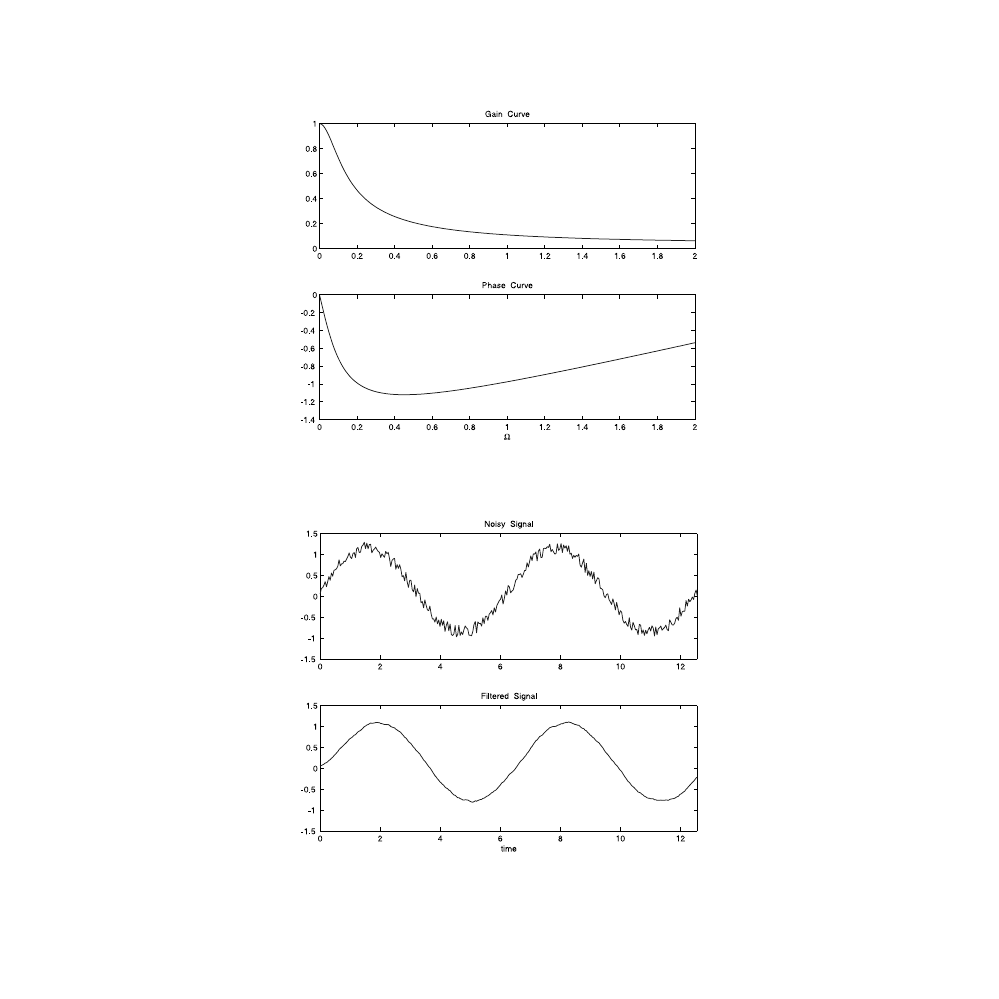
© 2001 by CRC Press LLC
FIGURE 6.4
The gain (top panel) and phase (bottom panel) responses of a low-pass filter as a function
of the frequency.
FIGURE 6.5
The action of a low-pass filter. Top panel: Profile of the signal contaminated by noise. Bottom
panel: Profile of the filtered signal.

© 2001 by CRC Press LLC
y(1)=u(1);
for k=2:N
y(k)=+0.9*y(k-1)+0.1*u(k);
end
subplot(2,1,1)
plot(t,u)
axis([0 4*pi -1.5 1.5]);
title('Noisy Signal')
subplot(2,1,2)
plot(t,y)
title('Filtered Signal')
axis([0 4*pi -1.5 1.5]);
Application 3
The digital prototype bandpass filter ideally filters out from a signal all fre-
quencies lower than a given frequency and higher than another frequency. In
practice, the cutoffs are not so sharp and the lower and higher cut-off frequen-
cies of the bandpass are defined as those at which the gain curve (i.e., the mag-
nitude of the Transfer Function as function of the frequency) is at
its
maximum value.
The difference equation that describes this prototype filter is
(6.115)
where
Ω
0
is the normalized frequency with maximum gain and r is a number
close to 1.
The purpose of the following analysis is, given the lower and higher cutoff
normalized frequencies, to find the quantities
Ω
0
and r in the above difference
equation.
The Transfer Function for the above difference equation is given by:
(6.116)
where
(6.117)
( /
)
1
2
y k
r
r
r u k
r
y k
r y k
( ) {(
)
cos(
)
} ( )
cos(
) (
)
(
)
=
−
−
+
+
− −
−
1
1 2
2
2
1
2
0
2
0
2
Ω
Ω
H z
g z
z
r
z r
( )
cos(
)
=
−
+
0
2
2
0
2
2
Ω
g
r
r
r
0
0
2
1
1 2
2
= −
−
+
(
)
cos(
)
Ω

© 2001 by CRC Press LLC
and
z = e
j
Ω
The gain of this filter, or equivalently the magnitude of the Transfer Function, is
(6.118)
where
(6.119)
(6.120)
The lower and upper cutoff frequencies are defined, as previously noted, by
the condition:
(6.121)
Substituting condition (6.121) in the gain expression (6.118) leads to the con-
clusion that the cutoff frequencies are obtained from the solutions of the fol-
lowing quadratic equation:
(6.122)
Adding and subtracting the roots of this equation, we deduce after some
straightforward algebra, the following determining equations for
Ω
0
and r:
1. r is the root in the interval [0, 1] of the following eighth-degree
polynomial:
(6.123)
where
(6.124)
H e
r
r
r
Ar Br
Ar
r
j
(
)
(
)
cos(
)
(
)
Ω
Ω
=
−
−
+
+
+
+
+
1
1 2
2
1
0
2
2
3
4
A
= −4
0
cos( ) cos(
)
Ω
Ω
B
=
+
−
4
4
2
2
2
0
cos ( )
cos (
)
Ω
Ω
H e
j
(
)
( , )
Ω
1 2
1
2
=
cos ( )
(
) cos(
)
cos( )
(
)
[
cos(
) (
) ] cos (
)
2
2
0
2
2
0
2
2
0
1
1
4
4
2
1
0
Ω
Ω
Ω
Ω
Ω
−
+
+ −
− −
+
=
r
r
r
r
r
r
r
a b r
ar
a
b
r
ar
a b r
8
6
5
4
3
2
8
14
2
2
8
1 0
+ −
−
+
−
−
−
+ −
+ =
(
)
(
)
(
)
a
=
+
(cos(
) cos(
))
Ω
Ω
1
2
2

© 2001 by CRC Press LLC
(6.125)
2.
Ω
0
is given by:
(6.126)
Example 6.12
Write a program to determine the parameters r and
Ω
0
of a prototype band-
pass filter if the cutoff frequencies and the sampling time are given.
Solution:
The following script M-file implements the above target:
f1= ;
%enter the lower cutoff
f2= ;
%enter the upper cutoff
tau= ;
%enter the sampling time
w1=2*pi*f1*tau;
w2=2*pi*f2*tau;
a=(cos(w1)+cos(w2))^2;
b=(cos(w1)-cos(w2))^2;
p=[1 0 a-b -8*a 14*a-2*b-2 -8*a a-b 0 1];
rr=roots(p);
r=rr(find(rr>0 & rr<1 & imag(rr)==0))
w0=acos((r*a^(1/2))/(1+r^2));
f0=(1/(2*pi*tau))*w0
, we show the gain and phase response for this filter, for the
case that the cutoff frequencies are chosen to be 1000 Hz and 1200 Hz, and the
sampling rate is 10
µs.
To test the action of this filter, we input into it a signal that consists of a mix-
ture of a sinusoid having a frequency at the frequency of the maximum gain
of this filter and a number of its harmonics; for example,
(6.127)
We show in
the input and the filtered signals. As expected from
an analysis of the gain curve, only the fundamental frequency signal has sur-
vived. The amplitude of the filtered signal settles to that of the fundamental
frequency signal following a short transient period.
NOTE
Before leaving this topic, it is worth noting that the above prototype
bandpass filter can have sharper cutoff features (i.e., decreasing the value of
b
=
−
(cos(
) cos(
))
Ω
Ω
1
2
2
Ω
0
1
1 2
2
1
=
+
−
cos
/
ra
r
u t
f t
f t
f t
( )
sin(
)
. sin(
)
. sin(
)
=
+
+
2
0 5
4
0 6
6
0
0
0
π
π
π
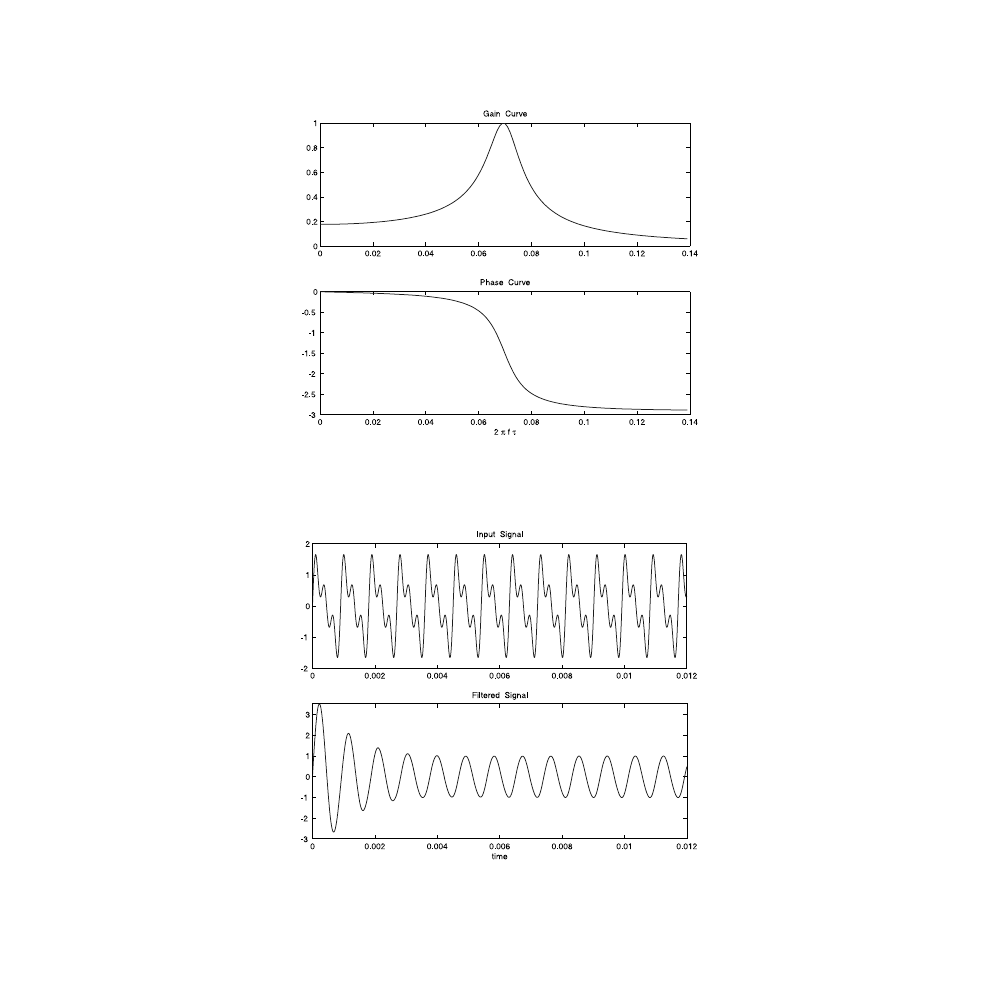
© 2001 by CRC Press LLC
FIGURE 6.6
The transfer function of a prototype bandpass filter. Top panel: Plot of the gain curve as
function of the normalized frequency. Bottom panel: Plot of the phase curve as function of
the normalized frequency.
FIGURE 6.7
The filtering action of a prototype bandpass filter. Top panel: Input signal consists of a
combination of a fundamental frequency signal (equal to the frequency corresponding to
the filter maximum gain) and two of its harmonics. Bottom panel: Filtered signal.

© 2001 by CRC Press LLC
the gain curve for frequencies below the lower cutoff and higher than the
upper cutoff) through having many of these prototype filters in cascade. This
will be a topic of study in future linear system or filter design courses.
In-Class Exercises
Pb. 6.59
Work out the missing algebraic steps in the derivation leading to
Eqs. (6.123) through (6.126).
Pb. 6.60
Given the following values for the lower and upper cutoff frequen-
cies and the sampling time:
f
1
= 200 Hz; f
2
= 400 Hz;
τ = 10
–5
s
find f
0
and plot the gain curve as function of the normalized frequency for the
bandpass prototype filter.
6.10 MATLAB Commands Review
abs
Computes the modulus of a complex number.
angle
Computes the argument of a complex number.
conj
Computes the complex conjugate of a complex number.
find
Finds the locations of elements in an array that satifies certain
specified conditions.
imag
Computes the imaginary part of a complex number.
real
Computes the real part of a complex number.
Document Outline
- ELEMENTARY MATHEMATICAL and COMPUTATIONAL TOOLS for ELECTRICAL and COMPUTER ENGINEERS USING MATLAB ®
- Table of Contents
- Chapter Six
- Complex Numbers
- 6.1 Introduction
- 6.2 The Basics
- 6.3 Complex Conjugation and Division
- 6.4 Polar Form of Complex Numbers
- 6.5 Analytical Solutions of Constant Coefficients ODE
- 6.6 Phasors
- 6.7 Interference and Diffraction of Electromagnetic Waves
- 6.8 Solving ac Circuits with Phasors: The Impedance Method
- 6.9 Transfer Function for a Difference Equation with Constant Coefficients*
- 6.10 MATLAB Commands Review
- Complex Numbers
Wyszukiwarka
Podobne podstrony:
1080 PDF C09
1080 PDF C07
1080 PDF C08
instr 2011 pdf, Roztw Spektrofoto
więcej podobnych podstron