Capacity and Flow

Optimization

Lecture Outline

• Introduction
• Bifurcated Flows with Linear Function
• Routing Restrictions
• Link Modularity
• Example
• Convex Function
• Concluding Remarks

Lecture Outline

• Introduction

• Bifurcated Flows with Linear Function
• Routing Restrictions
• Link Modularity
• Example
• Convex Function
• Concluding Remarks

Introduction (1)

• Network design problems called also capacity

and flow assignment (CFA) problems are one of

the most frequently encountered problems in

network optimization

• They are used in the case when a new network is

designed or an existing network is

incremented

• The objective is usually network cost defined as

the cost of network links and other network

performance metrics (e.g., delay, survivability)

• According to the modeled computer network,

various kinds of multicommodity flows with a range

of constraints are used

CFA Problems

• Bifurcated multicommodity flows

– Linear objective
– Convex objective
– Modularity

• Non-bifurcated multicommodity flows

– Linear objective
– Convex objective
– Modularity

Lecture Outline

• Introduction

• Bifurcated Flows with Linear Function

• Routing Restrictions
• Link Modularity
• Example
• Convex Function
• Concluding Remarks

Bifurcated Flows - Linear Function

(1)

• CFA (Capacity and Flow Assignment) problem
• Bifurcated unicast flows (e.g., IP protocol)
• Objective is to minimize network cost function
• Both link-path and node-link formulations can

be used

Bifurcated Flows - Linear Function

(2)

Given: network topology, unicast demands,

candidate paths

Minimize: network cost (linear)

Over: bifurcated flows (routing), link capacity

Link-Path Formulation (1)

indices
d = 1,2,…,D

demands

p = 1,2,…,P

d

candidate paths for demand d

e = 1,2,…,Elinks
constants



edp

= 1, if link e belongs to path p realizing

demand d; 0, otherwise

h

d

volume of demand d



e

unit (marginal) cost of link e

Link-Path Formulation (2)

variables
x

dp

flow allocated to path p of demand d

(continuous

non-negative)

y

e

capacity of link e (continuous non-negative)

objective
minimize F = 

e



e

y

e

constraints


p

x

dp

= h

d

, d = 1,2,…,D



d



p



edp

x

dp

 y

e

, e = 1,2,…,E.

Shortest Path Allocation Rule

• Since the link capacity variable y

e

is continuous,

for optimal solution the capacity constraint is
binding, i.e., the link flow must be equal to the link
capacities (otherwise, the objective includes cost
of an unused capacity)

F = 

e



e

y

e

= 

e



e



d



p



edp

x

dp

= 

d



p

x

dp



e



edp



e

= 

d



p



dp

x

dp

• For each demand, allocate its entire demand

volume to its shortest path, with respect to links
unit costs and candidate path. If there is more
than one shortest path for a demand then the
demand volume can be split among the shortest
paths in an arbitrary way

Decoupled Link-Path

Formulation

variables
x

dp

flow allocated to path p of demand d

(continuous
non-negative)

objective
minimize F = 

d



p



dp

x

dp

constraints


p

x

dp

= h

d

, d = 1,2,…,D.

The solution yields shortest path algorithm applied for

each demand

Node-Link Formulation (1)

indices
d = 1,2,…,D

demands

e = 1,2,…,Elinks
v = 1,2,…,Vnodes
constants
a

ev

= 1, if link e originates at node v; 0, otherwise

b

ev

= 1, if link e terminates in node v; 0,

otherwise

h

d

volume of demand d



e

unit (marginal) cost of link e

Node-Link Formulation (2)

constants
s

d

source node of demand d

t

d

destination node of demand d

variables
x

ed

flow of demand d sent on link e (continuous

non-negative)

y

e

capacity of link e (continuous non-negative)

Node-Link Formulation (3)

objective
minimize F = 

e



e

y

e

constraints


e

 a

ev

x

ed

 – 

e

 b

ev

x

ed

 =  h

d

,   if v = s

d

v = 1,2,…,V

d = 1,2,…,D



e

 a

ev

x

ed

 – 

e

 b

ev

x

ed

 = –h

d

,   if v = t

d

v = 1,2,…,V

d = 1,2,…,D



e

 a

ev

x

ed

 – 

e

 b

ev

x

ed

 = 0,  if v  s

d

,t

d

v = 1,2,…,V

d = 1,2,…,D



d

x

ed

 y

e

, e = 1,2,…,E.

Formulation Comparison (1)

• V – number of nodes, P – average number of

candidate paths, k – average number of adjacent
nodes, V



(V) – number of demand origin nodes

Formulation

Number of

variables

Number of constraints

Link-path

PxV



(V



1 )+0.5kxV

=O(V

2

)

PxV



(V



1 )+0.5kxV

=O(V

2

)

Node-link

0.5kxVxV



(V



1 )x

=O(V

3

)

VxV



(V



1 )+0.5kxV

=O(V

3

)

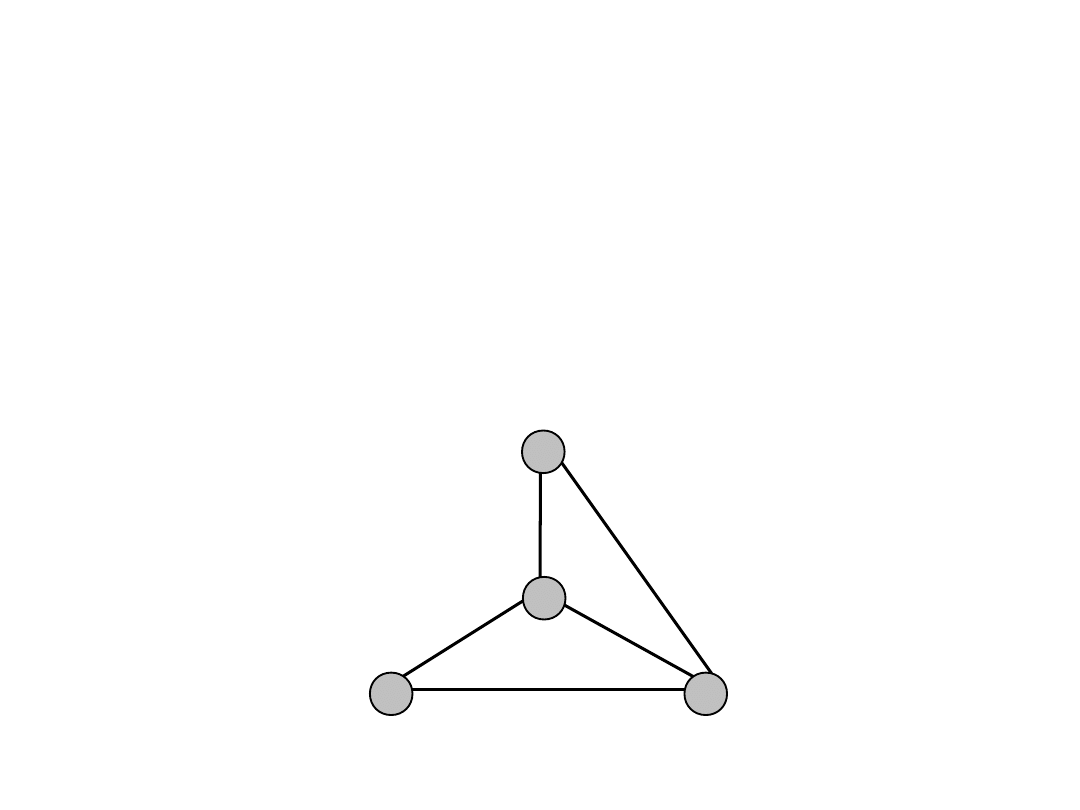
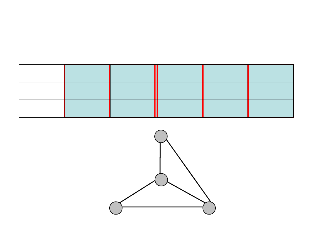
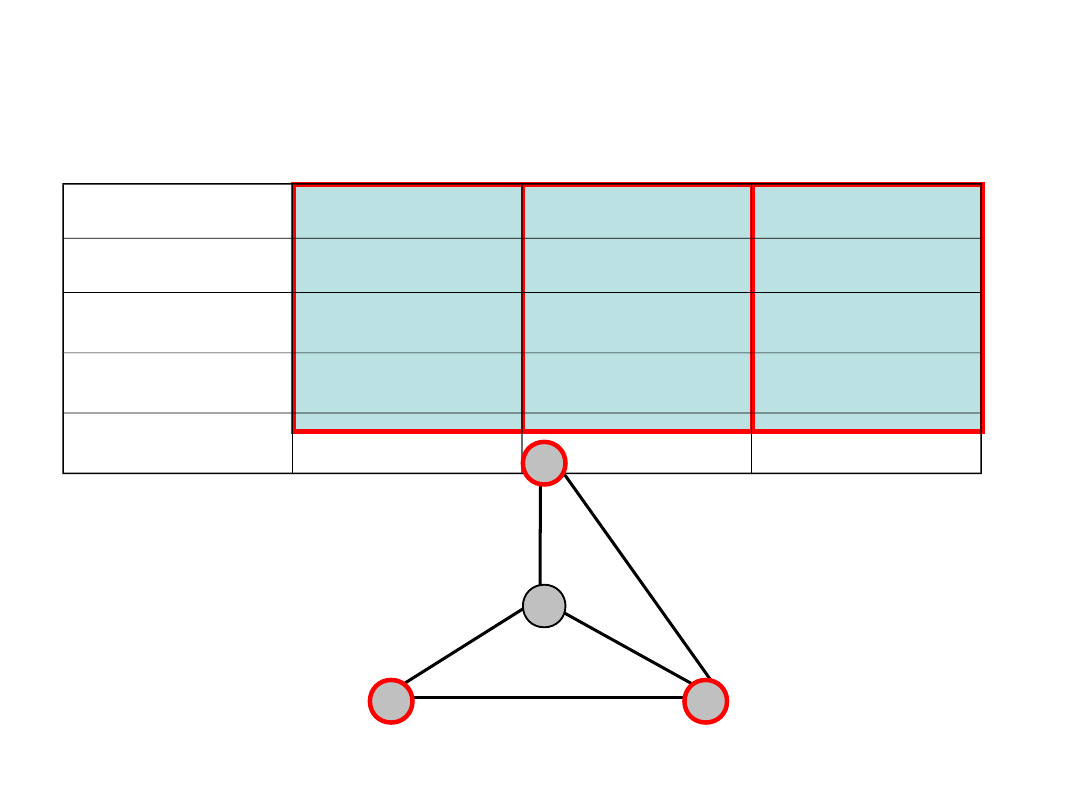
Example (1)

• The network consits of 4 nodes and 5 links
• There are 3 demands between nodes 1-2, 1-3, 2-3
• Link-path notation

1

3

4

2

e=1

e=2

e=5

e=4

e=3

Example (2)

1

3

4

2

Link

e = 1

e = 2

e = 3

e = 4

e = 5

Node

2-3

2-4

3-4

1-4

1-3

Cost



1

= 2



2

= 1



3

= 1



4

= 3



5

= 1

e=1

e=2

e=5

e=4

e=3

Example (3)

Demand

1

2

3

Nodes

1-2

1-3

2-3

Volume

h

1

= 15

h

2

= 20

h

3

= 10

Path

P

11

={2,4}

P

21

={5}

P

31

={1}

Pat

P

22

={3,4}

P

32

={2,3}

1

3

4

2

e=1

e=2

e=5

e=4

e=3

Example (4)

e=1

e=2

e=5

e=4

e=3

link/path P

11

={2,4

}

P

21

={5} P

22

={3,4

}

P

31

={1} P

32

={2,3

}

e = 1

0

0

0

1

0

e = 2

1

0

0

0

1

e = 3

0

0

1

0

1

e = 4

1

0

1

0

0

e = 5

0

1

0

0

0

1

4

2

3

Example (5)

minimize
F = 2y

1

+ y

2

+ y

3

+ 3y

4

+ y

5

constraints
x

11

+ x

21

+ x

22

+ x

31

+ x

32

= 15 (h

1

)

x

11

+

x

21

+ x

22

+ x

31

+ x

32

= 20 (h

2

)

x

11

+ x

21

+ x

22

+

x

31

+ x

32

= 10 (h

3

)

x

11

+ x

21

+ x

22

+

x

31

+ x

32

 y

1

x

11

+ x

21

+ x

22

+ x

31

+ x

32

 y

2

x

11

+ x

21

+

x

22

+ x

31

+ x

32

 y

3

x

11

+ x

21

+ x

22

+ x

31

+ x

32

 y

4

x

11

+

x

21

+ x

22

+ x

31

+ x

32

 y

5

x

11

, x

21

, x

22

, x

31

,

x

32

 0,

y

1

, y

2

, y

3

, y

4

, y

5

 0

e

x

11

x

21

x

22

x

31

x

32

1

0

0

0

1

0

2

1

0

0

0

1

3

0

0

1

0

1

4

1

0

1

0

0

5

0

1

0

0

0

Incremental Network Design

(1)

• CFA (Capacity and Flow Assignment) network

extension problem

• Bifurcated unicast flows (e.g., IP protocol)
• Objective is to minimize network cost of

additional capacity added to the network

• Link-path formulation

Incremental Network Design

(2)

Given: network topology, unicast demands,

candidate paths, link capacity

Minimize: network extension cost (linear)

Over: bifurcated flows (routing), additional link

capacity

Incremental Network Design

(2)

indices
d = 1,2,…,D

demands

p = 1,2,…,P

d

candidate paths for demand d

e = 1,2,…,Elinks
constants



edp

= 1, if link e belongs to path p realizing

demand d; 0, otherwise

h

d

volume of demand d

c

e

capacity of link e



e

unit (marginal) cost of link e

Incremental Network Design

(3)

variables
x

dp

flow allocated to path p of demand d

(continuous

non-negative)

y

e

additional capacity of link e (continuous non-

negative)

objective
minimize F = 

e



e

y

e

constraints


p

x

dp

= h

d

, d = 1,2,…,D



d



p



edp

x

dp

 c

e

+ y

e

, e = 1,2,…,E.

Optimization

• Network design problems with linear cost and

bifurcated flowscan be solve by the Simplex
method

• For larger networks heuristics can be applied

Lecture Outline

• Introduction
• Bifurcated Flows with Linear Function

• Routing Restrictions

• Link Modularity
• Example
• Convex Function
• Concluding Remarks

Path Diversity (1)

• CFA (Capacity and Flow Assignment) problem
• Bifurcated unicast flows
• Objective is to minimize network cost function
• Link-path formulation
• Path diversity requirement to force splitting

demand volumes into more than one path

Path Diversity (2)

Given: network topology, unicast demands,

candidate paths, diversity factor for each demand

Minimize: network cost (linear)

Over: bifurcated flows (routing), link capacity

Path Diversity (3)

indices
d = 1,2,…,D

demands

p = 1,2,…,P

d

candidate paths for demand d

e = 1,2,…,Elinks
constants



edp

= 1, if link e belongs to path p realizing

demand d; 0, otherwise

h

d

volume of demand d



e

unit (marginal) cost of link e

n

d

diversity factor for demand d

Path Diversity (3)

variables
x

dp

flow allocated to path p of demand d (continuous

non-negative)

y

e

capacity of link e (continuous non-negative)

objective
minimize F = 

e



e

y

e

constraints


p

x

dp

= h

d

, d = 1,2,…,D



d



p



edp

x

dp

 y

e

, e = 1,2,…,E

x

dp

≤ h

d

/n

d

, d= 1,2,...,D p = 1,2, ...,P

d

.

Single Path Routing (1)

• CFA (Capacity and Flow Assignment) problem
• Objective is to minimize network cost function
• Link-path formulation
• Single path routing, i.e., Non-bifurcated flows

Single Path Routing (2)

Given: network topology, unicast demands,

candidate paths

Minimize: network cost (linear)

Over: Non-bifurcated flows (routing), link capacity

Single Path Routing (3)

variables (additional)
u

dp

binary variable corresponding to the flow

allocated

to path p of demand d

objective
minimize F = 

e



e

y

e

constraints
x

dp

= h

d

u

dp

, d = 1,2,…,D p = 1,2,…,P

d



p

u

dp

= 1, d = 1,2,…,D



d



p



edp

x

dp

 y

e

, e = 1,2,…,E.

Optimization

• With continuous capacity the problem can be

solved by Shortest Path Allocation Rule

• With integer capacity the the single path problem

is linear, integer (binary) and NP-complete

(equivalent to non-bifurcated flow problem)

• To find optimal solution branch-and-bound or

branch-and-cut algorithm must be constructed

• The solution process can be divided into two

phases: capacity assignment and flow

assignment, i.e., Top-Down approach

• Heuristics can be used, e.g., Flow Deviation,

evolutionary algorithm, etc.

Lecture Outline

• Introduction
• Bifurcated Flows with Linear Function
• Routing Restrictions

• Link Modularity

• Example
• Convex Function
• Concluding Remarks

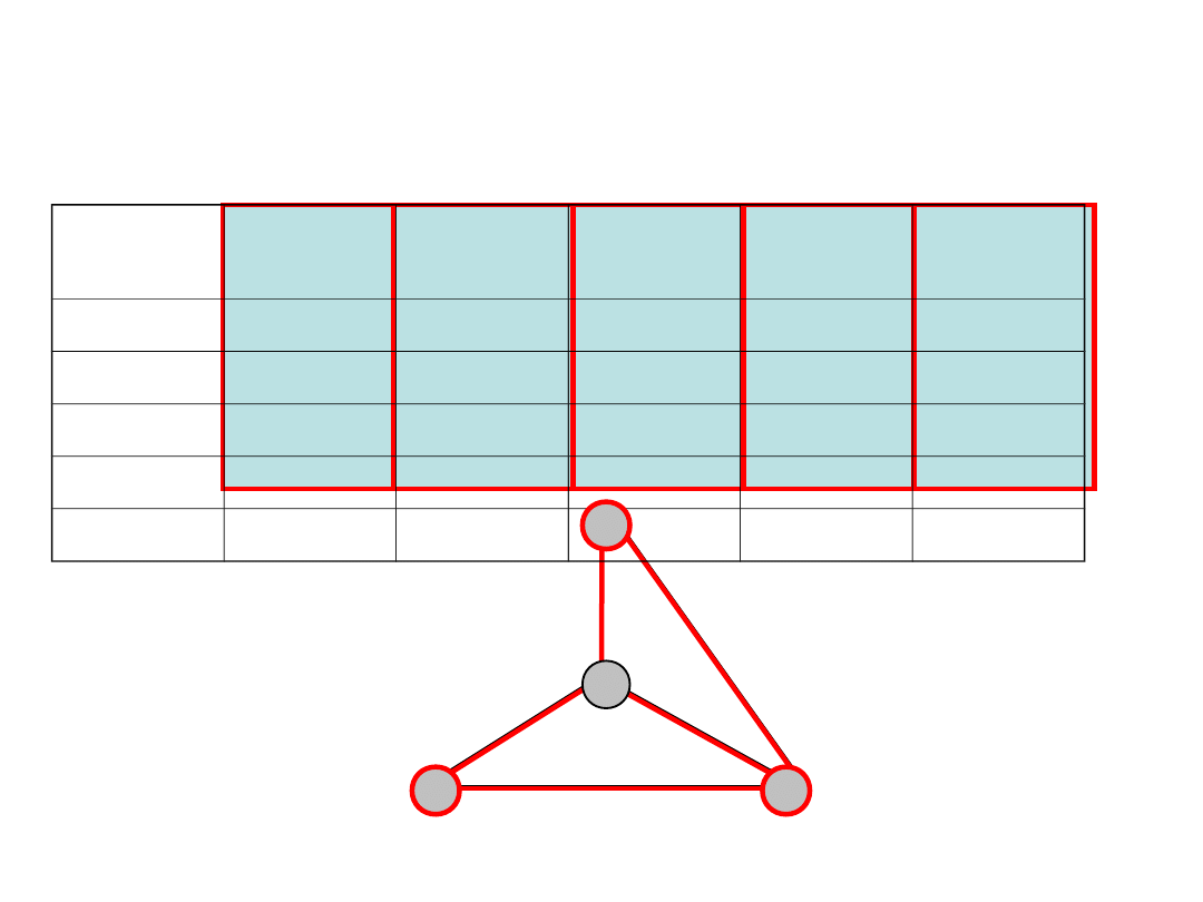
Link Modularity (1)

• Link modularity is a common feature in

communications networks, i.e., link capacity must
be a multiple of particular module of capacity

• Link modularity follows from technological

constraints, e.g., SDH/SONET, WDM

• To include link modularity condition in the model,

the link capacity variable must be integer

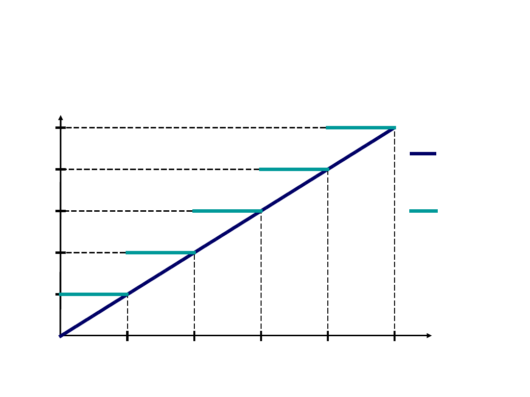
Link Modularity (2)

Link load

Link cost

M

2M

3M

4M

5M

Continuous
link capacity

Modular
link capacity

Modular Links Problem (1)

• CFA (Capacity and Flow Assignment) problem
• Bifurcated unicast flows (e.g., IP protocol)
• Objective is to minimize network cost function
• Modular link modeling
• Link-path formulation

Modular Links Problem (2)

Given: network topology, unicast demands,

candidate paths, link modules

Minimize: network cost (linear)

Over: bifurcated flows (routing), link capacity

Modular Links Problem (3)

indices
d = 1,2,…,D

demands

p = 1,2,…,P

d

candidate paths for demand d

e = 1,2,…,Elinks
constants



edp

= 1, if link e belongs to path p realizing

demand d; 0, otherwise

h

d

volume of demand d



e

cost of one capacity module on link e

M

size of the link capacity module

Modular Links Problem (4)

variables
x

dp

flow allocated to path p of demand d

(continuous
non-negative)

y

e

capacity of link e as the number of modules (non-
negative integer)

objective
minimize F = 

e



e

y

e

constraints


p

x

dp

= h

d

, d = 1,2,…,D



d



p



edp

x

dp

 My

e

, e = 1,2,…,E.

Optimization

• The modular links problem is linear, integer and

NP-complete

• To find optimal solution branch-and-bound or

branch-and-cut algorithm must be constructed

• The solution process can be divided into two

phases: capacity assignment and flow
assignment, i.e., Top-Down approach

• Heuristics can be used, e.g., Flow Deviation,

evolutionary algorithm, etc.

Candidate Link Capacity (1)

• In some cases the telecoms propose to customers

a set of possible candidate links, e.g., DSL links
in the Internet access

• Each candidate link has a fixed capacity
• The customer is to select one of the candidate

links

• Usually, the cost of a capacity unit (e.g., 1

Mbps) decrases with the increase of the
candidate link capacity, i.e., the cost function is
concave

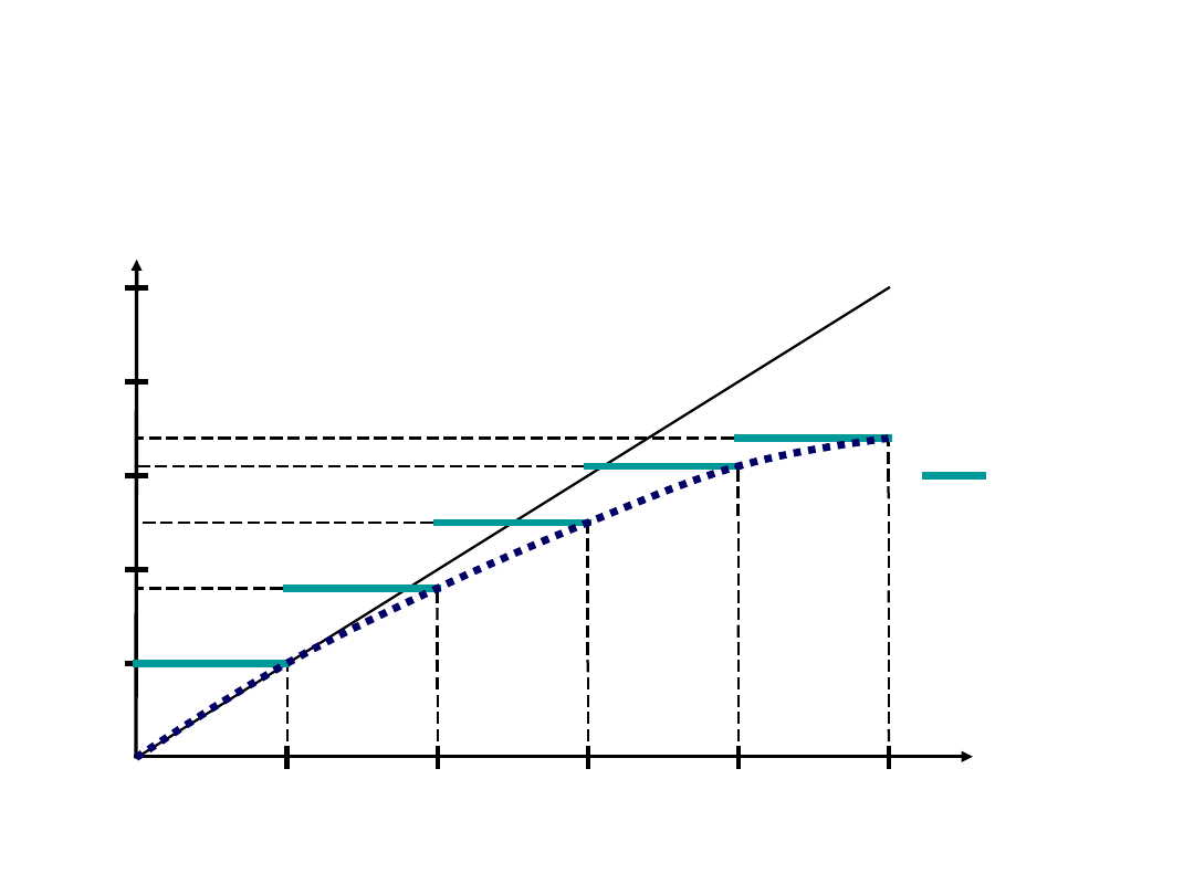
Candidate Link Capacity (2)

Link load

Link cost

M

2M

3M

4M

5M

Candidate
link capacity

Candidate Links Problem (1)

• CFA (Capacity and Flow Assignment) problem
• Bifurcated unicast flows (e.g., IP protocol)
• Objective is to minimize network cost function
• Candidate link modeling
• Link-path formulation

Candidate Links Problem (2)

Given: network topology, unicast demands,

candidate paths, candidate links

Minimize: network cost (linear)

Over: bifurcated flows (routing), link capacity

Candidate Links Problem (3)

indices (additional)
k = 1,2,…,K

e

candidate link types for link e

constants (additional)



ek

cost of candidate link type k on link e

c

ek

capacity of candidate link type k on link e

variables
x

dp

flow allocated to path p of demand d

(continuous
non-negative)

y

ek

= 1, if link type k is selected for link e; 0,

otherwise

Candidate Links Problem (4)

objective
minimize F = 

e



k



ek

y

ek

constraints


p

x

dp

= h

d

, d = 1,2,…,D



k

y

ek

= 1, e = 1,2,…,E



d



p



edp

x

dp

 

k

c

ek

y

ek

, e = 1,2,…,E.

Optimization

• The modular links problem is linear, integer

(binary) and NP-complete

• To find optimal solution branch-and-bound or

branch-and-cut algorithm must be constructed

• The solution process can be divided into two

phases: capacity assignment and flow
assignment, i.e., Top-Down approach

• Heuristics can be used, e.g., Flow Deviation,

evolutionary algorithm, etc.

Lecture Outline

• Introduction
• Bifurcated Flows with Linear Function
• Routing Restrictions
• Link Modularity

• Example

• Convex Function
• Concluding Remarks

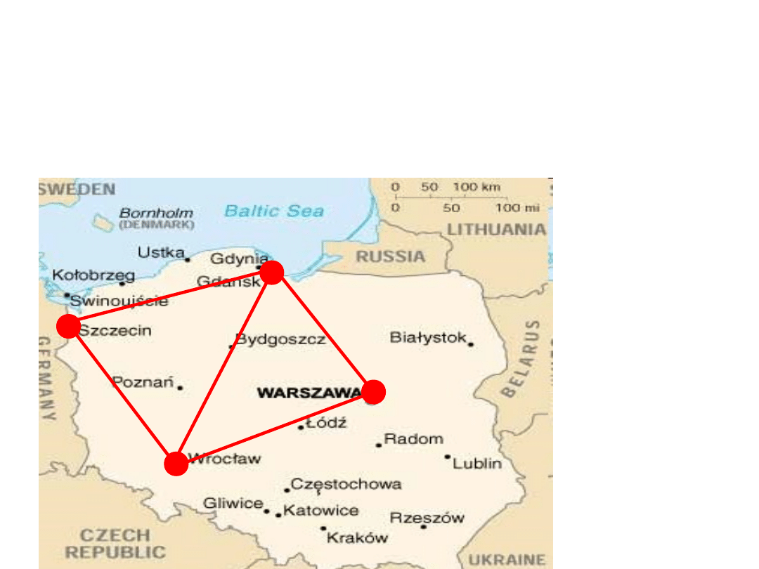
Example (1)

1

2

3

4

Szczecin-Gdańsk
<1,2> c=? Mbps
<2,1> c=? Mbps
Szczecin-Wrocław
<1,3> c=? Mbps
<3,1> c=? Mbps
Gdańsk-Wrocław
<2,3> c=? Mbps
<3,2> c=? Mbps
Gdańsk-
Warszawa
<2,4> c=? Mbps
<4,2> c=? Mbps
Wrocław-
Warszawa
<3,4> c=? Mbps
<4,3> c=? Mbps

???

???

???

???

???

Demands (node pairs):
• Szczecin (1) – Warszawa (4) (demand value x)
• Gdańsk (2) – Wrocław (3) (demand value y)
• Wrocław (3) – Warszawa (4) (demand value v)

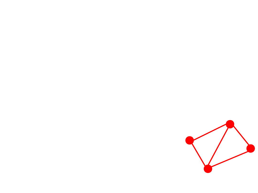
1

2

3

4

Example (2)

• Link-path notation
Candidate paths
• x1={1,2,4}; x2={1,3,4}; x3={1,2,3,4};

x4={1,3,2,4}

• y1={2,3}; y2={2,1,3}; y3={2,4,3}
• v1={3,4}; v2={3,2,4}; v3={3,1,2,4}
Constraints
• x: x1 + x2 + x3 +x4 = x
• y: y1 + y2 + y3 = y
• v: v1 + v2 + v3 = v

1

2

3

4

Example (3)

• Integer link capacity variables are denoted as c12, c21,

etc.

• The capacity module is 2 Mbps, only for links 34 and 43

it is 1 Mbps

Link costs:
• Szczecin-Gdańsk <1,2> 700 euro/month for 2 Mbps
• Szczecin-Wrocław <1,3> 900 euro/month for 2 Mbps
• Gdańsk-Wrocław <2,3> 800 euro/month for 2 Mbps
• Gdańsk-Warszawa <2,4> 500 euro/month for 2 Mbps
• Wrocław-Warszawa <3,4> 400 euro/month for 1 Mbps

Example (4)

Capacity constraints

• c12: x1 + x3 + v3 – 2c12 <= 0

• c21: y2 – 2c21 <= 0

• c13: x2 + x4 + y2 – 2c13 <= 0

• c31: v3 – 2c31 <= 0

• c23: x3 + y1 – 2c23 <= 0

• c32: x4 + v2 – 2c32 <= 0

• c24: x1 + x4 + y3 + v2 + v3 – 2c24 <= 0

• c42: - 2c42 <= 0

• c34: x2 + x3 + v1 – c34 <= 0

• c43: y3 – c43 <= 0

1

2

3

4

Example (5)

x1={1,2,4}; x2={1,3,4};
x3={1,2,3,4}; x4={1,3,2,4}
y1={2,3); y2={2,1,3};
y3={2,4,3}
v1={3,4}; v2={3,2,4};
v3={3,1,2,4}

Capacity constraints

0 <= c12 <= 3 (maximum 3 modules of 2 Mbps)
0 <= c21 <= 3
0 <= c13 <= 3
0 <= c31 <= 3
0 <= c23 <= 3
0 <= c32 <= 3
0 <= c24 <= 3
0 <= c42 <= 3
0 <= c34 <= 3 (maximum 3 modules of 1 Mbps)
0 <= c43 <= 3

1

2

3

4

Example (6)

• File cap1.lp
• Solution

c12 = 2 c21 = 0 c13 = 0 c31 = 0 c23 = 1
c32 = 0 c24 = 2 c42 = 0 c34 = 3 c43 = 1

• 700c12 + 700c21 + 900c13 + 900c31 + 800c23

+ 800c32 + 500c24 + 500c42 + 400c34 +
400c43 =
700x2 + 800x1 + 500x2 + 400x3 + 400 = 4800
euro/month

Example (7)

Maximum number of modules set to 4 (cap2.lp)
0 <= c12 <= 4 etc.
Solution: 4800 euro/month
Maximum number of modules set to 2 (cap3.lp)
0 <= c12 <= 2 etc.
Solution: 5600 euro/month
Maximum number of modules set to 2, capacity can

be continuous (not integer) (cap4.lp)

Solution: 4450 euro/month

Example (8)

Non-bifurcated flows
Maximum number of modules set to 2, capacity can be

continuous (cap5.lp)

Solution: None
Maximum number of modules set to 3, capacity can be

continuous (cap6.lp)

Solution: 4200 euro/month
Maximum number of modules set to 3, capacity integer

(cap7.lp)

Solution: 5200 euro/month

Example (9)

Lecture Outline

• Introduction
• Bifurcated Flows with Linear Function
• Routing Restrictions
• Link Modularity
• Example

• Convex Function

• Concluding Remarks

Convex Problem (1)

• CFA (Capacity and Flow Assignment) problem
• Non-bifurcated unicast flows
• Objective is to minimize function including

network delay and network cost function

• Candidate link modeling
• Link-path formulation

Convex Problem (2)

Given: network topology, unicast demands,

candidate paths, candidate links

Minimize: network delay + network cost

Over: Non-bifurcated flows (routing), link capacity

Convex Problem (3)

indices
d = 1,2,…,D

demands

p = 1,2,…,P

d

candidate paths for demand d

e = 1,2,…,Elinks
k = 1,2,…,K

e

candidate link types for link e

Convex Problem (4)

constants



edp

= 1, if link e belongs to path p of demand d; 0,

otherwise

h

d

volume of demand d



ek

cost of candidate link type k on link e

c

ek

capacity of candidate link type k on link e

variables
x

dp

1, if path p is used to realize demand d; 0,

otherwise

y

ek

= 1, if link type k is selected for link e; 0, otherwise

f

e

flow on link e (non-negative, continuous)

Convex Problem (5)

objective
minimize F = 

e

f

e

/(

k

c

ek

y

ek

– f

e

) + 

e



k



ek

y

ek

constraints


d



p



edp

h

d

x

dp

= f

e

e = 1,2,…,E



p

x

dp

= 1, d = 1,2,…,D



k

y

ek

= 1, e = 1,2,…,E

f

e

 

k

c

ek

y

ek

, e = 1,2,…,E.

Lagrangian Relaxation (1)

Since the objective function is increasing in f

e

, the

problem can be reformulated as

objective
minimize F = 

e

f

e

/(

k

c

ek

y

ek

– f

e

) + 

e



k



ek

y

ek

constraints



d



p



edp

h

d

x

dp

 f

e

, e = 1,2,…,E



p

x

dp

= 1, d = 1,2,…,D



k

y

ek

= 1, e = 1,2,…,E

0  f

e

 

k

c

ek

y

ek

, e = 1,2,…,E.

Lagrangian Relaxation (2)

Let  = [



1

,



2

,…,



E

] be a vector of Lagrangian

multipliers

Flow f

e

definition constraint is relaxed and the

corresponding Lagrangian function is as follows

L()=(

e

f

e

/(

k

c

ek

y

ek

– f

e

) + 

e



k



ek

y

ek

) + 

e



e

(

d



p



edp

h

d

x

dp

– f

e

)

= 

e

f

e

/(

k

c

ek

y

ek

– f

e

) + 

e



k



ek

y

ek

– 

e



e

f

e

+ 

e



d



p



edp



e

x

d

x

dp

Since variables f

e

and x

dp

are not linked, we receive D +

E subproblems, that can be solved independently

Lagrangian Relaxation (3)

First subproblem is formulated for variables x

dp

for

each link d = 1,2,…,D

objective
minimize L

d

() = 

e



p



edp



e

h

d

x

dp

constraints


p

x

dp

= 1.

To solve the problem, a shortest path p = 1,2,…,P

d

under the metric



e

must be find, using any

shortest path algorithm

Lagrangian Relaxation (4)

Second subproblem is formulated for variables y

ek

and f

e

for each link e = 1,2,…,E

objective
minimize L

e

() = f

e

/(

k

c

ek

y

ek

– f

e

) + 

k



ek

y

ek

–



e

f

e

constraints


k

y

ek

= 1,

0  f

e

 

k

c

ek

y

ek

.

Lagrangian Relaxation (5)

Since K

e

is relatively small for each link, we can solve

the problem for each k = 1,2,…,K

e

separately

objective
minimize L

e

(,k) = f

e

/(c

ek

– f

e

) +



ek

–



e

f

e

constraints
0  f

e

 c

ek

.

The solution is

Next the subgradient method can be applied




















ek

e

ek

e

e

ek

ek

e

c

λ

c

λ

λ

c

c

k

f

1

for

0

1

for

)

(

Lecture Outline

• Introduction
• Bifurcated Flows with Linear Function
• Routing Restrictions
• Link Modularity
• Example
• Convex Function

• Concluding Remarks

Concluding Remarks

• Network design problems problems are one of the

most popular problems in network optimization

• Network design problems with bifurcated flows

and continuous linear link costs can be solved by

standard optimization methods, e.g., Simplex

• Network design problems with Non-bifurcated

flows or/and modular links belong to the class of

MIP problems and to obtain optimal solution

branch and bound or branch and cut methods

must be applied, however only for small networks

• Capacity and flow assignment problems are mostly

simpler than corresponding flow assignment

problems

Further Reading

• M. Pióro, D. Medhi, Routing, Flow, and Capacity Design in

Communication and Computer Networks, Morgan Kaufman
Publishers 2004

• A. Kasprzak, Algorytmy równoczesnej optymalizacji

przepływów, przepustowości kanałów i struktur
topologicznych sieci teleinformatycznych, Wydawnictwo
Politechniki Wrocławskiej, Wrocław, 1989 (in polish)

• B. Gavish, S. Huntler, An Algorithm for Optimal Route

Selection in SNA Networks, IEEE Trans. Commun., Vol. COM-
31, No. 10, 1983, pp. 1154-1160

• B. Gavish, I. Neuman, A System for Routing and Capacity

Assignment in Computer Communication Networks, IEEE
Trans. Commun., Vol. 37, No. 4, 1989, pp. 360-366