
SYSTEMS OF LINEAR EQUATIONS I
and more on THE RANK OF A MATRIX.
Lecture 6

a
11
x
1
+ a
12
x
2
+ .....+ a
1n
x
n
=
b
1
a
21
x
1
+ a
22
x
2
+ .....+ a
2n
x
n
=
b
2
..............................................
.........................
a
n1
x
1
+ a
n2
x
2
+ .....+ a
nn
x
n
=
b
n
,
x
i
, i = 1, 2, ..., n; denote the unknowns;
a
ik
R; i, k = 1, 2, ..., n; denote the coefficients
b
i
R, i = 1, 2, ..., n; denote the constants
where
Let us consider the general form of the the system of n equations in n unknowns
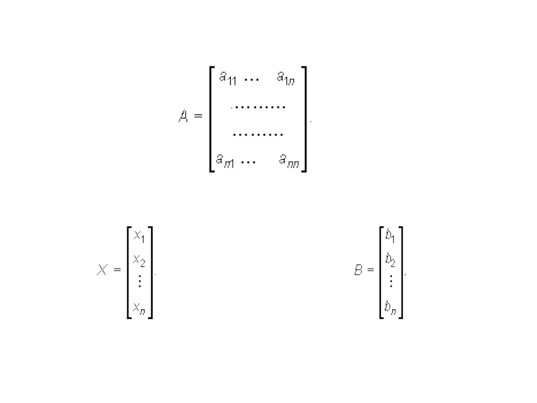
The coefficient matrix of the system of equations:
The column of unknowns: The columns of constants:
Remember the notation: Det A = |A|
Because the system is nonsingular, Det A 0, the inverse matrix A
-1
exists.
Both sides of the matrix equation are multiplied by A
-1
.
A X = B.
X = A
-1
B.
1. The matrix method
Assumption: Det A 0
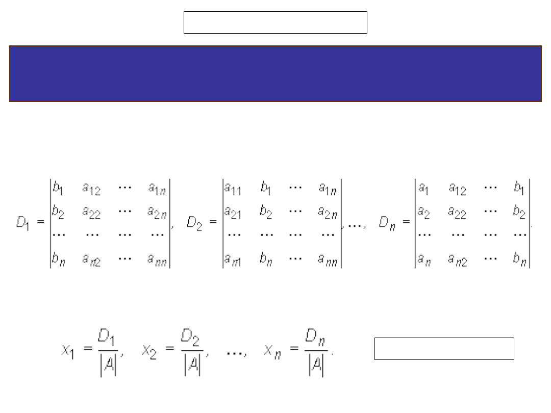
2. The Cramer’s Rule
Let D
i
be a matrix obtained from A by replacing its i-th column with the
column of the constants.
The solutions of the system are;
Definition
A Cramer's system is a system of equations for which det A 0 i.e. the
coefficient matrix A is nonsingular.
where |A| = Det A
,
0
0
1
0
0
1
)
(
,
1
0
0
0
0
1
)
(
,
1
0
0
1
0
0
)
(
1
2
1
z
y
x
X
I
z
y
x
X
I
z
y
x
X
I
33
3
31
23
2
21
13
1
11
33
33
32
31
31
23
23
22
21
21
13
13
12
11
11
2
a
b
a
a
b
a
a
b
a
a
z
a
y
a
x
a
a
a
z
a
y
a
x
a
a
a
z
a
y
a
x
a
a
I
A
2
2
2
)
(
D
Det
I
Det
A
Det
I
A
Det
y
I
Det
2
A
Det
D
Det
y
D
Det
y
A
Det
2
2
For a 3 x 3 system:
33
32
31
23
22
21
13
12
11
a
a
a
a
a
a
a
a
a
A
QED
Sketch of Proof
3
33
32
31
2
23
22
21
1
13
12
11
b
z
a
y
a
x
a
b
z
a
y
a
x
a
b
z
a
y
a
x
a
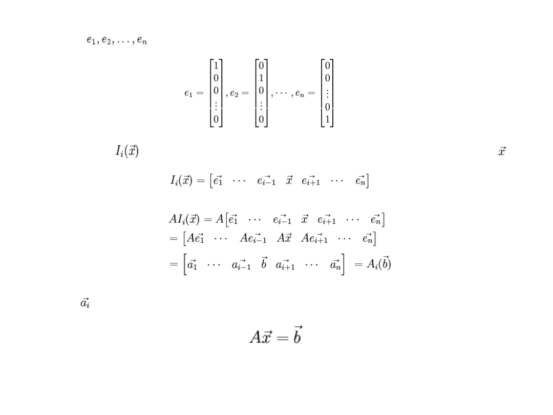
to be the n x n identity matrix with the i-th column replaced with the vector x
PROOF of the Cramers Rule
If we let
be columns of the n x n identity matrix, ie
and we define
ie
,
then it follows that
where is the ith column of the matrix A, produced by multiplying A by the ith column of the
identity matrix. Also note that we know
because this is the system we are considering solutions for.
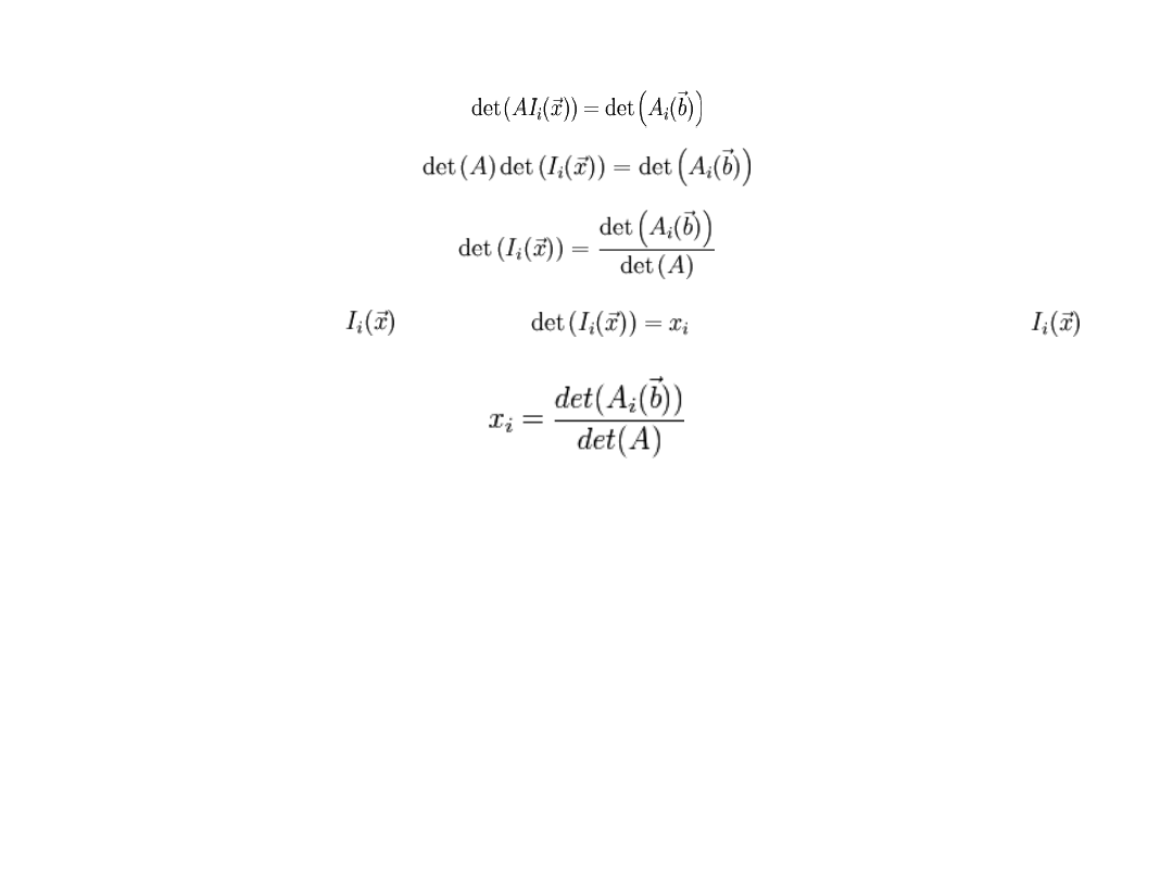
(expanding along the ith row of )
Taking the determinant of
we see that
thus
QED
Continuing, we take the determinant of both sides.
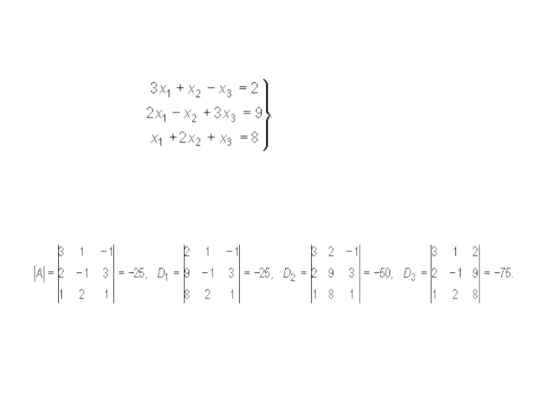
Solve the following system of equations
We calculate the successive determinants:
Thus: x
1
= 1, x
2
= 2, x
3
= 3.
Example

3. The Gaussian Elimination Method
Recall that it consists in performing on the augmented
matrix:
the following elementary operations:
•the interchange of two rows;
•the multiplication of every element of one row by a non zero
scalar k;
•the addition to the elements of one row, the corresponding
elements of another row multiplied by a non zero scalar k .
.
b
...
b
b
a
...
a
a
...
...
...
...
a
...
a
a
a
...
a
a
b
A
m
2
1
mn
2
m
1
m
n
2
22
21
n
1
12
11
n
2
1
nn
n
2
22
n
1
12
11
c
...
c
c
t
0
0
t
t
0
t
t
t
c
T
.
b
...
b
b
a
...
a
a
...
...
...
...
a
...
a
a
a
...
a
a
b
A
m
2
1
mn
2
m
1
m
n
2
22
21
n
1
12
11
Gaussian el.
I-st part
The process of Gaussian elimination has two parts.
The first part (Forward Elimination) reduces a given
system to either upper triangular form, or results in a
degenerate equation with no solution, indicating the system
has no solution.
The second step (Backward Elimination) uses back-
substitution to find the solution of the system above.
n
2
1
nn
22
11
s
...
s
s
d
0
0
0
d
0
0
0
d
s
D
n
2
1
nn
n
2
22
n
1
12
11
c
...
c
c
t
0
0
t
t
0
t
t
t
c
T
Gaussian el.
II-nd part

Gaussian Elimination Steps:
1.
Write the augmented matrix for the system of linear
equations.
2. Use elementary row operations on the augmented
matrix [
A|b
] to transform A into upper triangular
form.
If a zero is located on the diagonal, switch the
rows until a nonzero is in that place. If you are
unable to do so, stop; the system has either infinite
or no solutions
.
3. Use back substitution to find the solution of the
problem.
Gaussian elimination:
1. Forward Elimination
Example
4
4
0
0
4
2
1
0
1
1
1
2
R
R
3
8
2
3
0
4
2
1
0
1
1
1
2
R
R
R
R
3
7
1
2
2
1
1
2
6
1
1
1
2
3
2
3
1
2
1
2. Backward subsitution
1
1
0
0
2
0
1
0
1
0
0
1
R
4
/
1
R
R
2
/
1
4
4
0
0
2
0
1
0
2
0
0
2
R
4
/
1
R
R
4
4
0
0
2
0
1
0
0
0
1
2
R
R
2
/
1
R
R
4
/
1
4
4
0
0
4
2
1
0
1
1
1
2
3
2
1
3
1
2
2
3
1
3


NOTE
The matrix method and the Cramers Rule work
only for nonsingular square systems,
the Gaussian Elimination is for any rectangular system.

Operation counts
CRAMERS RULE OPERATION COUNT
If we use the Laplace expansion to calculate the determinants
the Cramers Rule requires
(n+1)! multiplications
Comparison
Suppose that the system consists of 15 equations.
The Cramers Rule requires 15! ~ 4922789888000 ~ 5 ·10
12
multiplications,
if the mashine does 10
6
multiplications per second, then
it has to work about
one year.
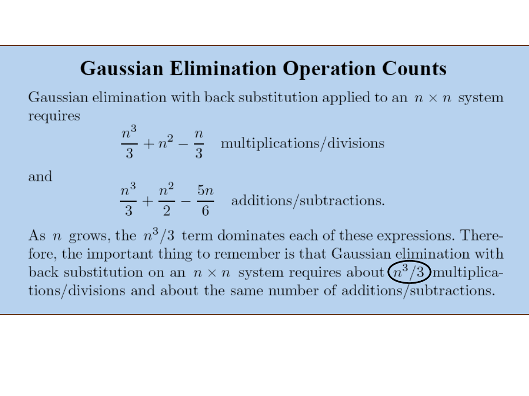
The Gaussian Elimination reqiures n
3
/3 + n
2
– n/3 = 1345 muliplications,
if it the mashine does the same number of multiplications, then
it works
about ~0.01 second.

OPERATION COUNTS FOR INVERSION
Computing A
-1
by reducing [ A| I ] with Gaussian Elimination
requires
•
n
3
multiplications/divisions
• n
3
- 2n
2
+ n additions/subtractions
Using A
-1
to solve a nonsingular system AX = b requires about
three times the effort as does Gaussian elimination with back substitution.
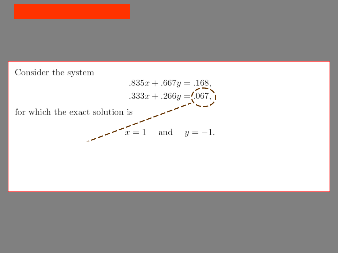
Ill-conditioning of a
system
Caution (IN NUMERICS)
How about 'checking the error' for ill-conditioned systems?
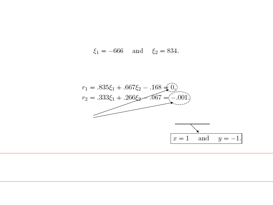
Let the solution of the above system be the slightly perturbed one:
If we substitute the values into the original system then:
!!!!!! It seems that the error is small !!!!! but from the exact result we know it isn't
HORROR,
we are not able to distinguish the correct
results
Example of Kahan
1440
.
0
8642
.
0
y
x
1441
.
0
2161
.
0
8648
.
0
2969
.
1
An approximate solution is
x
app
= 0.9911, y
app
=
-0.4870
And the error
r
:
8
8
app
10
10
y
x
1441
.
0
2161
.
0
8648
.
0
2969
.
1
1440
.
0
8642
.
0
X
A
b
r
b
x
A
Note that:
10
-8
= 0.00000001
The exact solution is
x = 2, y
= -2
THE CONDITION NUMBER C = ||A||·||A
-1|
| is very large
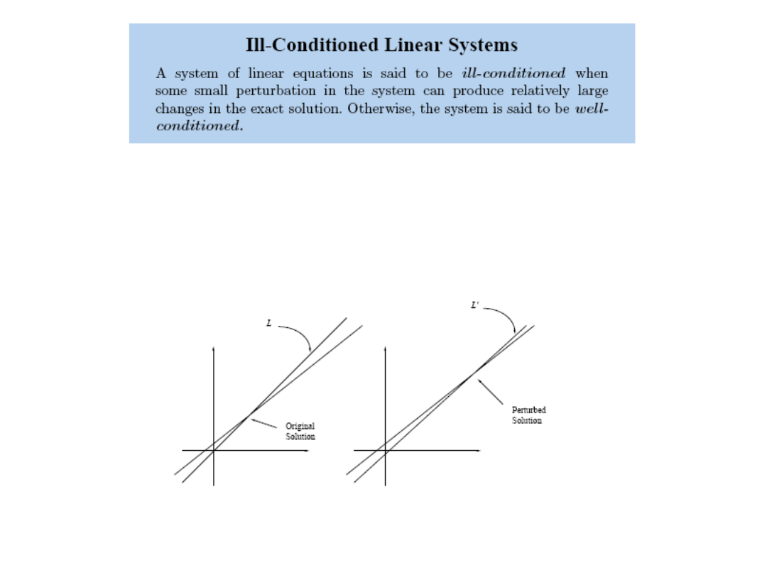
For 2 x 2 equations the ill-conditioned system can be interpreted as the
intersection of two straight lines almost parellel to each other.


The rank, consistency –
summary
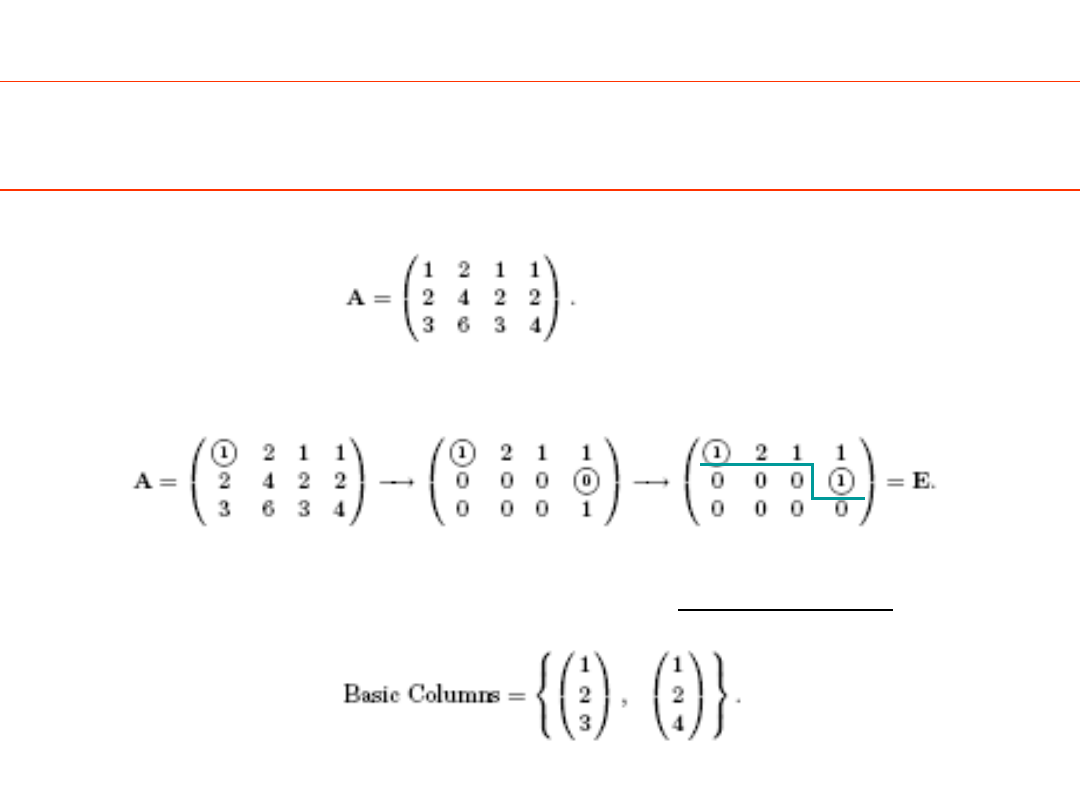
Definition
The rank of a matrix A is the number of nonzero rows in the row echelon form E of
the matrix
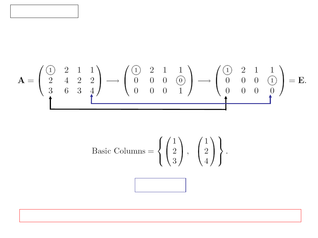
Example
We reduce A to row echelon form:
The rank of A is rank(A)=2. We also find the basic columns;
Definition
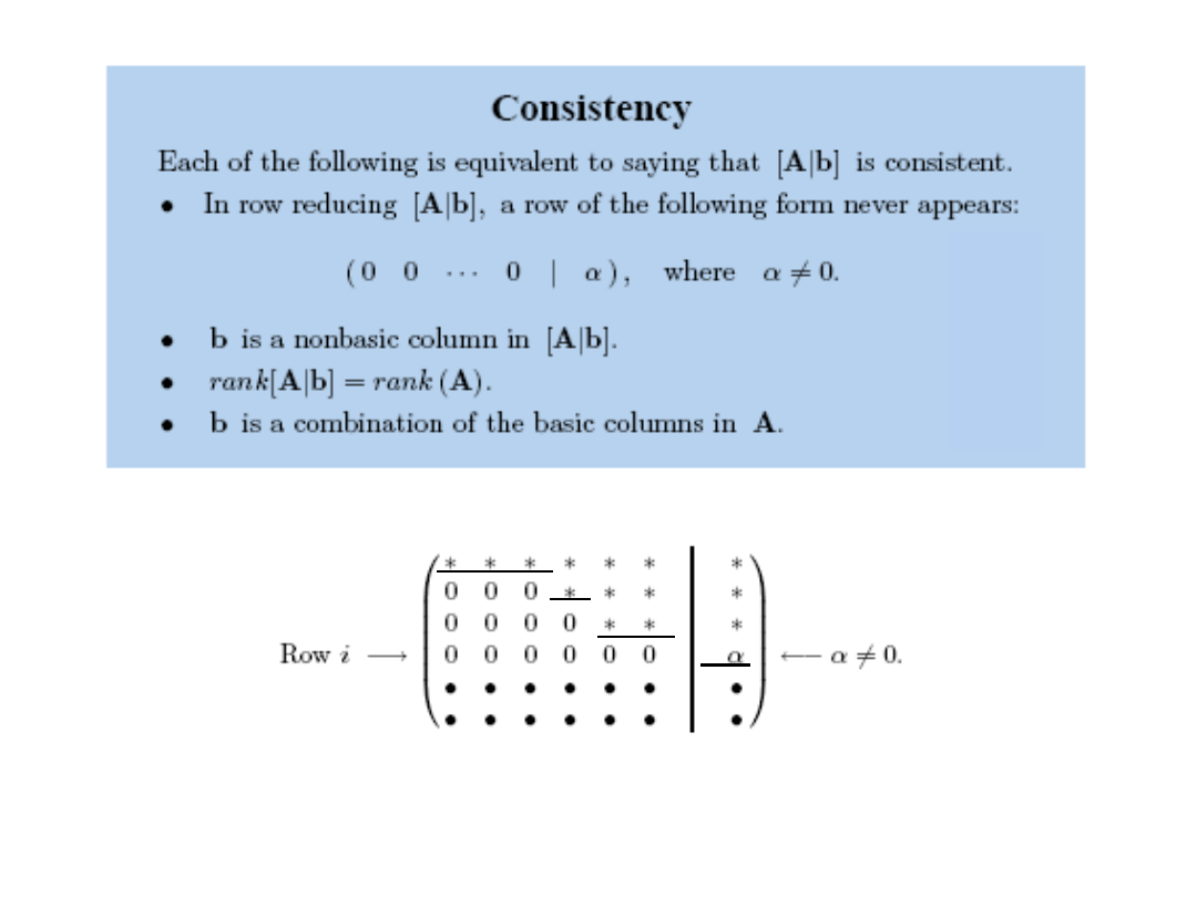
A system is said to be consistent if it possesses at least one solution.
If there are no solutions the system is said to be inconsistent.
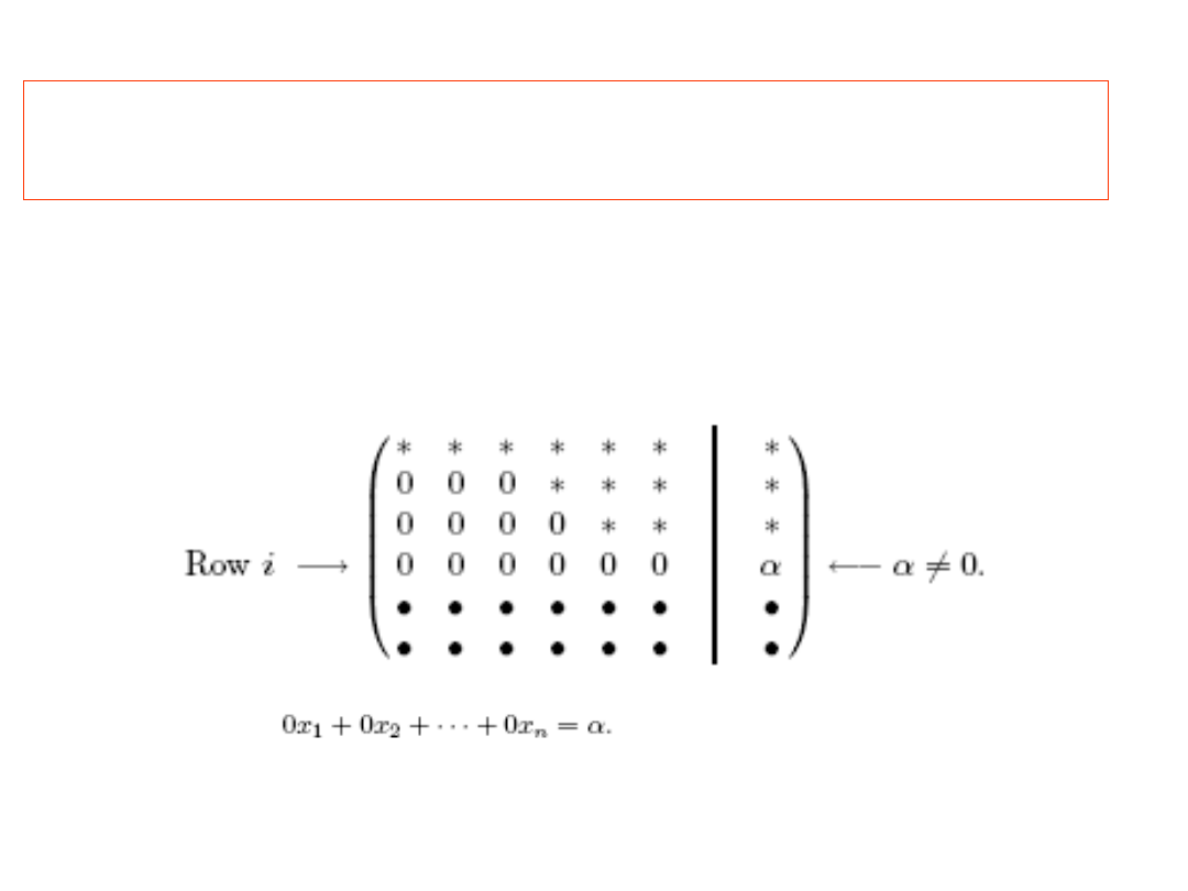
A good way to establish consistency of a system is to use Gaussian elimination.
Suppose that somewhere in the reduction process
For row i:
thus there are no solutions to
the original system.
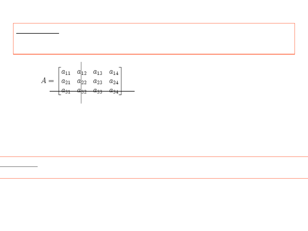
Definition
A submatrix of A is formed by removing whole columns or rows from
the original matrix.
Let
then some submatrix is
24
23
21
14
13
11
a
a
a
a
a
a
Definition
A kk minor determinant of A is the determinant of a k k square submatrix of A

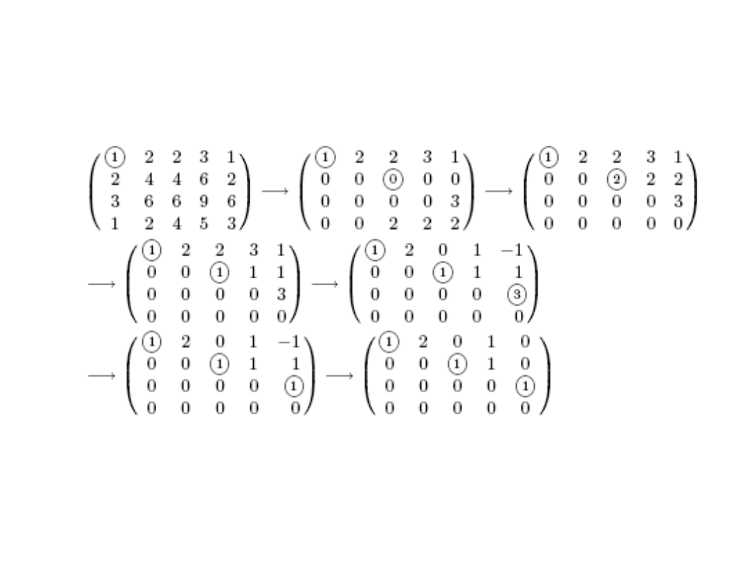
A new method to find the rank
Example
We reduce the marix to row echelon form:
There are two leading lements, so rank(A) = 2, and
Note that the basic columns are extarcted from A not from E.
rank A =2
Known Method
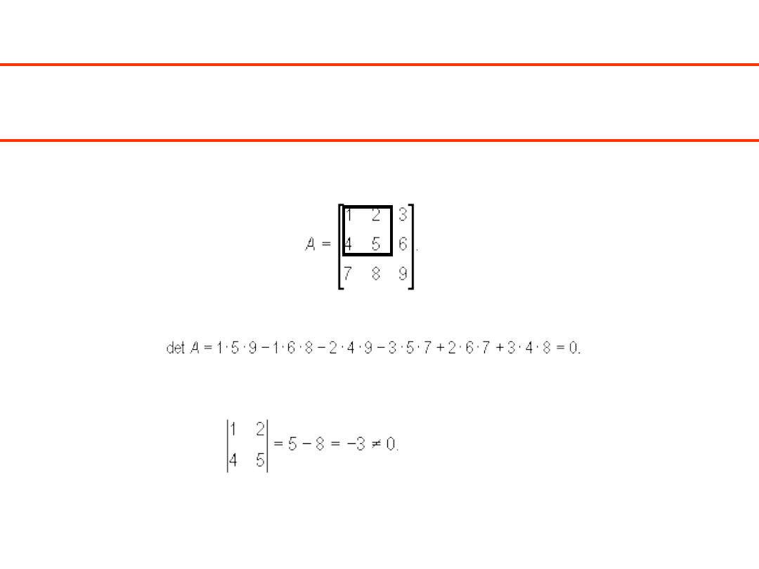
Theorem
The rank of a matrix is the order of the greatest non-vanishing minor in the matrix.
(the rank is zero when the matrix has all zero coefficients)
Find the rank of
We calculate the determinant :
Can we find a 22 nonsingular submatrix
determinant?
Yes,
We found a minor of order 2 different from 0, thus the
rank of A is equal 2.

Theorem
The rank of the matrix does not change if:
1) the columns are interchanged;
2) the columns are multiplied by numbers different from
0;
3) a linear combination of some columns is added to
another one;
4) the matrix is transposed.
One useful application of calculating the rank of a matrix is the
computation of the number of solutions of a
.
The KRONECKER-CAPELLI THEOREM
The system has at least one solution if the rank
of the coefficient matrix equals the rank of
augmented matrix.
In that case, it has precisely one solution if the rank
equals the number of equations;
otherwise, the general solution has k free
parameters where k is the difference between the
number of equations and the rank.
Document Outline
- Slide 1
- Slide 2
- Slide 3
- Slide 4
- Slide 5
- Slide 6
- Slide 7
- Slide 8
- Slide 9
- Slide 10
- Slide 11
- Slide 12
- Slide 13
- Slide 14
- Slide 15
- Slide 16
- Slide 17
- Slide 18
- Slide 19
- Slide 20
- Slide 21
- Slide 22
- Slide 23
- Slide 24
- Slide 25
- Slide 26
- Slide 27
- Slide 28
- Slide 29
- Slide 30
- Slide 31
- Slide 32
- Slide 33
- Slide 34
- Slide 35
Wyszukiwarka
Podobne podstrony:
L 7 Systems of linear equations II
Barret et al Templates For The Solution Of Linear Systems Building Blocks For Iterative Methods [s
THE USUI SYSTEM OF REIKI
Hamilton W R On quaternions, or on a new system of imaginaries in algebra (1850, reprint, 2000)(92s)
Modeling complex systems of systems with Phantom System Models
Lumiste Tarski's system of Geometry and Betweenness Geometry with the Group of Movements
Eugen Sandow System of physical training (2)
System Of A Down
07 System of government
,,DAMB Computer system of dynamic anal
„SAMB” Computer system of static analysis of shear wall structures in tall buildings
07 british system of governmrnt
Nieniemcki 7 Unit.!, Rock & Metal, System of a Down
Intro 2 Lorenz's System of EQs 03 Record p13
POZNAN 2, DYNAMICS OF SYSTEM OF TWO BEAMS WITH THE VISCO - ELASTIC INTERLAYER BY THE DIFFERENT BOUN
Hix The Political System of the EU rozdz 1
Jones D System of Enochian Magick 1
system of law
więcej podobnych podstron