Page 1

Development of probabilistic

climate predictions for UKCIP08

David Sexton,

James Murphy, Mat Collins, Geoff Jenkins , Glen

Harris, Kate Brown , Robin Clark, Penny Boorman, Simon Brown,

Richard Jones, Jason Lowe, Ben Booth, B. Bhaskaran, David Hassell,

Ruth McDonald, Tom Howard, Lizzie Kennett

UEA, October 19, 2007

Page 2

Content

 UKCIP08

 Probabilistic climate prediction system

 Modelling uncertainty and perturbed

physics ensembles

 Weighting with observations
 Time Scaling
 Other components of Earth System
 Downscaling

 Assumptions

Page 3

UKCIP ‘02

Based on the state-of-the-

art at the time - HadCM3,
HadAM3H time-slice, 50km
HadRM3 experiments

Used by many private and

public-sector organisations
to make decisions and
spend money

“Scenario” based with no

quantification of
uncertainties (although
plenty of caveats pointing
this out)

Page 4

Emission scenarios

Effects of internal
variability

Modelling of
Earth
system
processes

Uncertainties in model projections

… which
includes
how
informative
are models
about
reality

Page 5

Modelling uncertainty

Set of international climate models are

all ‘tuned’ to observations

But there is no guarantee these are the

actual optimal models

Other choices of values for model input

parameters could have provided equally

plausible simulations of observations

whilst providing a wide range of

responses in the future

So tuning could affect the decisions

planners make based on climate

predictions

Page 6

UKCIP08 – Probabilistic predictions

To provide joint probability distribution

functions (pdfs) of predicted changes in a
selection of key UK climate variables at
25km resolution for 2010-2039, 2020-
2049,…,2070-2099

Results will be presented for each

variable by month

We aim to deliver the final report and the

pdfs October 2008

Page 7

UKCIP08 Products

Report

Three types of output:

Probabilistic PDF
Weather Generator (change factors from PDFs)
Raw daily data from 17 regional climate models

Web-based data delivery package (UI)

Will produce nice graphics
Provide some analysis
Provide some guidance

Documentation on guidance

Preparatory workshops

Page 8

Probabilistic climate predictions are …

It is not a probability distribution from which the

real world samples what it does

So not an ensemble weather forecast for the

future.

It is just a representation of the degree to which

each possible future climate is plausible given

the evidence (climate models and observations).

As the evidence changes so will the prediction.

Underlying value is to reduce the risk of a user

making a bad decision

So instead of giving a policy maker all our

modelled and observed data we give them a

summary statement of the extent to which

various possible future climates are consistent

with the evidence.

Page 9

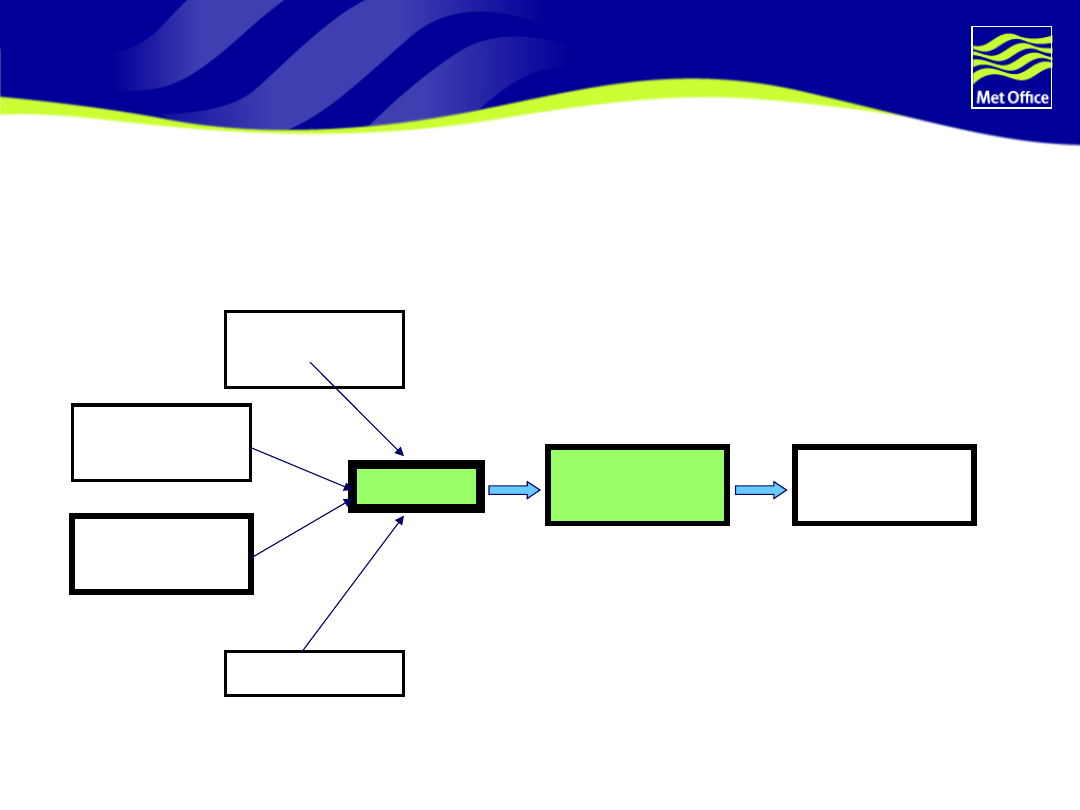
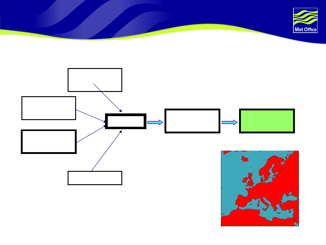
Production of UKCIP08 predictions

EBM

Time-
scaling

Down-
scaling

Perturbed
physics
ensemble

Ocean PPE

Aerosol
PPE

Carbon
cycle PPE

No computer in world is big enough to run many variants of a 25km
Earth system model so we have developed a framework to combine
lots of pieces (Murphy et al, Phil. Trans. Royal Society, 2007).

Page 10

Perturbed physics ensembles

Page 11

..use “perturbed physics ensembles” to sample
systematically a space of possible model configurations

• Relatively large ensembles designed to sample
modelling uncertainties systematically within a
single model framework

• Executed by perturbing model input parameters
controlling key model processes, within expert-
specified ranges

•

Key strength

: Allows greater control over

experimental design cf multi-model “ensembles of
opportunity”

•

Key limitation

: does not sample “structural

modelling uncertainties”, e.g. changes in resolution,
or in the fundamental assumptions used in the
model’s parameterisation schemes – need to include
results from other models to account for these.

Page 12

First steps

•Take one climate model (in this case

version 3 of the Hadley Centre model)

•Specify distributions for multiple

uncertain model parameters controlling

atmospheric physical processes

• Run an ensemble of simulations

(@300km horizontal resolution) of the

equilibrium response to doubled CO

Page 13

..gives a large (~300 member) sample of possible
changes (e.g. summer UK rainfall)

Page 14

Making

probabilistic

climate predictions

for 2xCO2

response

Page 15

Bayesian prediction – Goldstein and Rougier

Aim is to construct joint probability

distribution p(X, m

, m

,y,o,d) of all

uncertain objects in problem.

Input parameters (X)
Historical Model output (m

)

Model prediction (m

)

True climate (y

)

Observations (o)
Model imperfections (d)

It measures how all objects are related in

a probabilistic sense

Page 16

Best-input assumption

Physical and dynamical processes in a climate

model are controlled by numbers called model

input parameters.

We assume that one choice of these values, x*,

is better than all others

( *)

f x

True climate

Discrepancy

Model output
of best choice
of parameter
values x*

Page 17

Best-input assumption

We only know the probability that any

combination of parameter values is the

best-input model. But that means we

need millions of model variants.

That is too expensive - can only afford

hundreds of runs but they have to

sampled in a way that is consistent with

your beliefs about where the best model

is.

Need a cheap alternative..

Page 18

Emulators e.g. climate sensitivity

Ensemble member

lim

sit

ity

)

Dots – actual runs

Lines – 95% credible
interval from emulator

Emulators are statistical
models, trained on
ensemble runs, designed to
predict model output at
untried parameter
combinations

Page 19

Sampling different model variants with
emulator

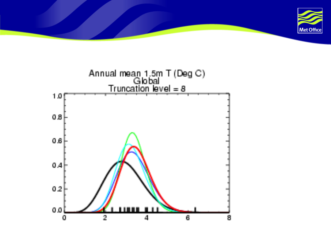
Page 20

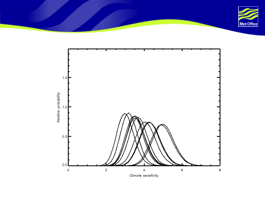
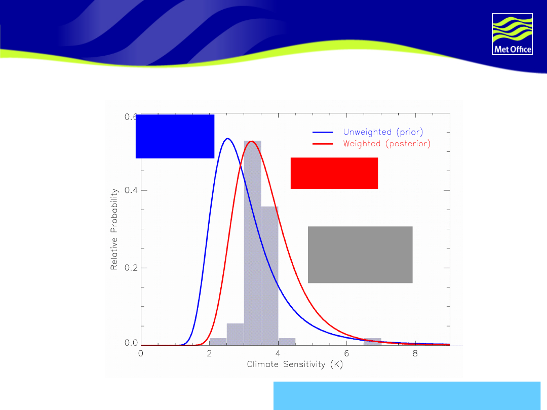
Climate sensitivity – before weighting with
observations

FOCUS
ON
BLACK
CURVE

The
Prior

Page 21

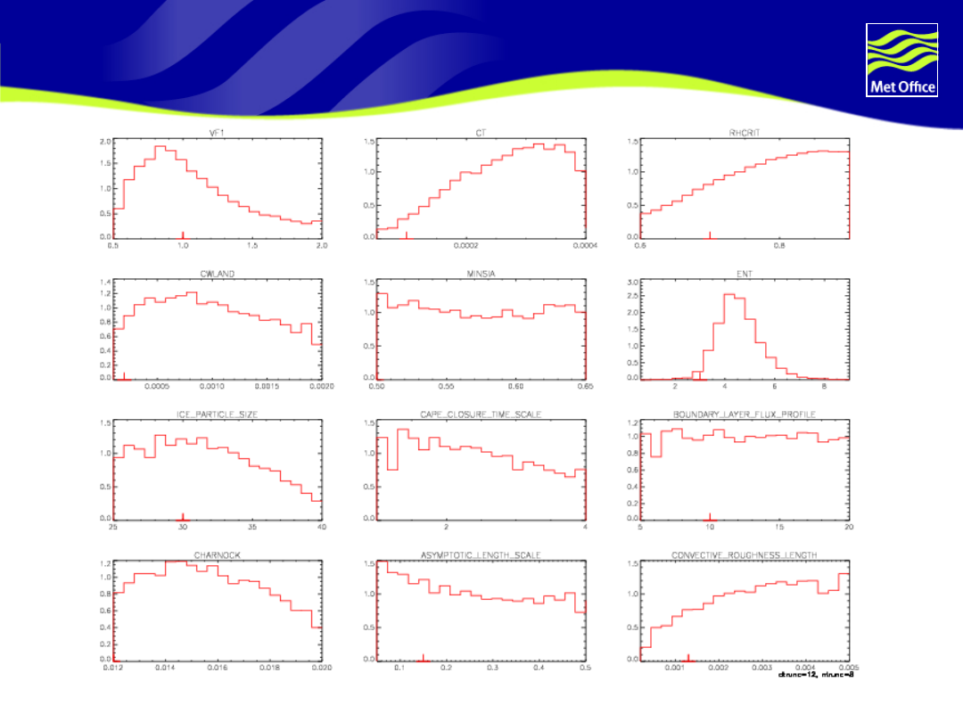
Parameter Constraints due to
weighting

Page 22

Weighting different model variants

Page 23

Weighting different model variants

Page 24

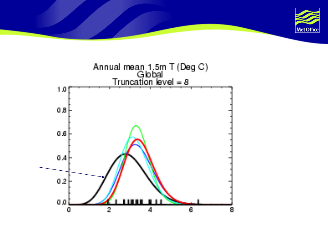
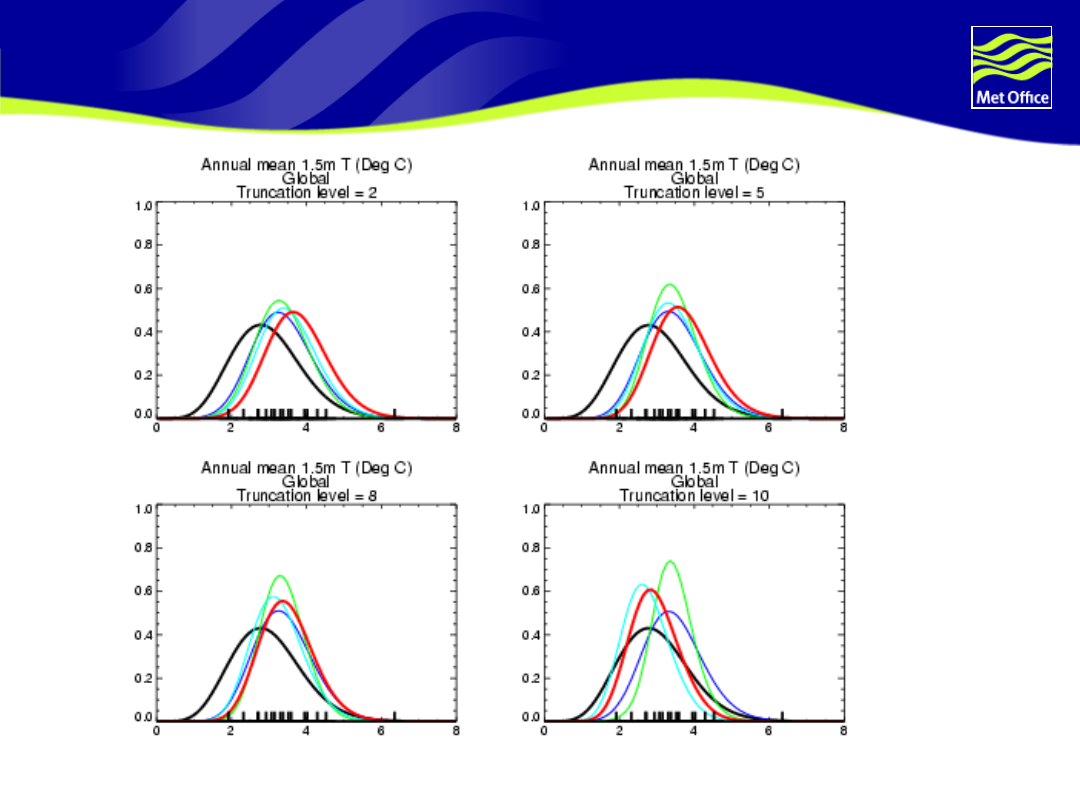
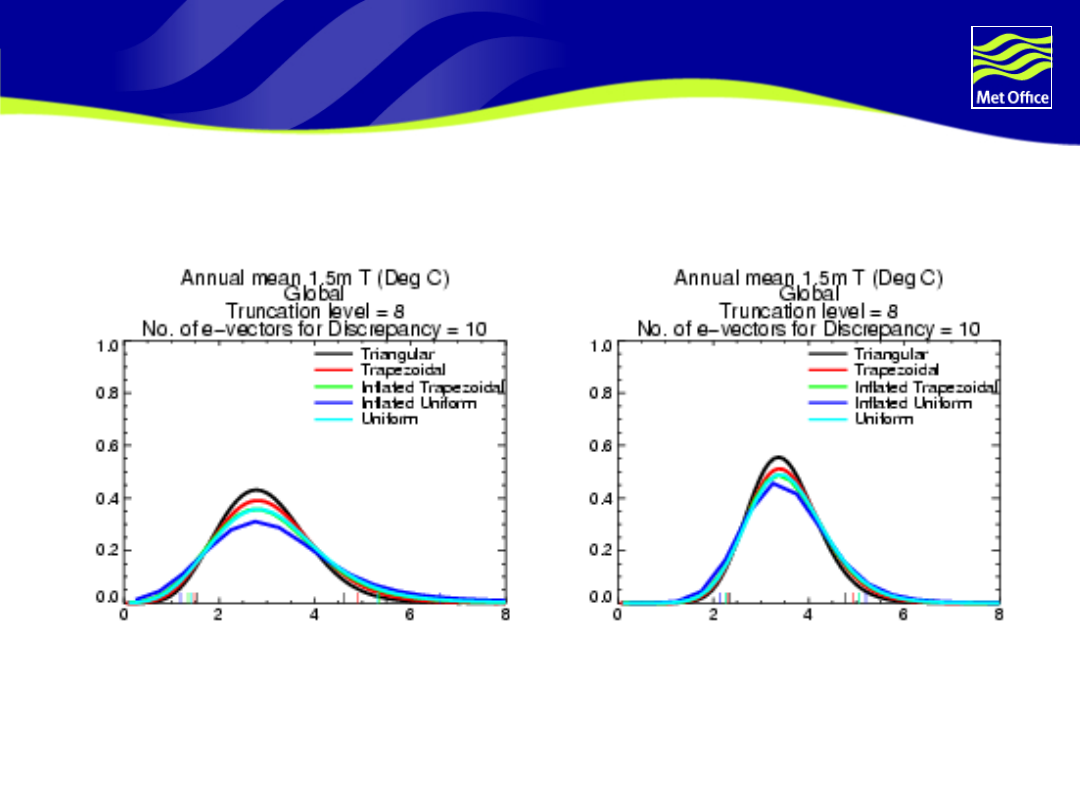
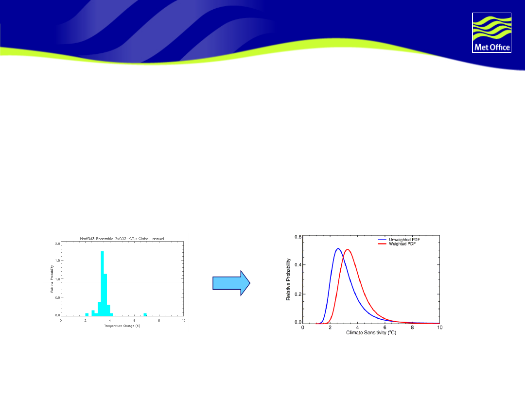
Climate sensitivity

“Truncation
level” =
amount of
independent
information
from
observations

FOCUS
ON
RED
CURVE

The
Posteri
or

Page 25

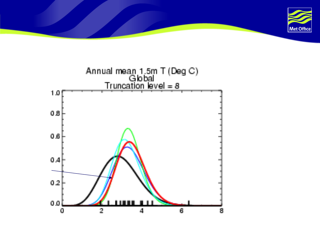
Climate sensitivity

“Truncation
level” =
amount of
independent
information
from
observations

FOCUS
ON
RED
CURVE

Page 26

Weighting models

with observations

and discrepancy

Page 27

Physics/dynamics matter…

Compare models against several

observational variables – with just one

variable you can simulate climate well for

the wrong reasons

Will compare with present-day mean

climate - Indirect assessment of key

processes for our climate prediction but

adds confidence to our prediction of one-

off event

We are not going to assume models are

perfect so using better models has an

impact

Page 28

Best-input assumption

Physical and dynamical processes in a climate

model are controlled by numbers called model

input parameters.

We assume that one choice of these values, x*,

is better than all others

( *)

f x

True climate

Discrepancy

Model output
of best choice
of parameter
values x*

Page 29

Comparing models with observations

Use likelihood function i.e. skill of model is

likelihood of model data given some observations

log ( )

log| |

(

)

(

)

=- -

m-o V m-o

V = obs uncertainty + emulator error +

discrepancy

Discrepancy

is ‘distance’ between real system and

‘best’ choice of input parameters

Truncation level

= dimensionality of m, o

Page 30

Discrepancy – a schematic of what
it does

•Avoids observations over-constraining the pdfs.
•Avoids contradictions from subsequent

analyses when some observations have been

allowed to constrain the problem too strongly.

Page 31

Specifying discrepancy

Use multimodel ensemble from AR4 and

CFMIP

For each multimodel ensemble member,

find emulated model variant that is

closest to that member

There is a distance between climates of

this multimodel ensemble member and

this “best” emulated model variant i.e.

effect of processes not explored by slab

model variants.

Pool these distances over all multimodel

ensemble members

Page 32

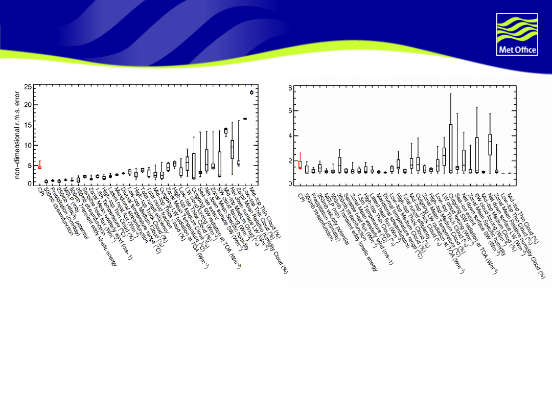
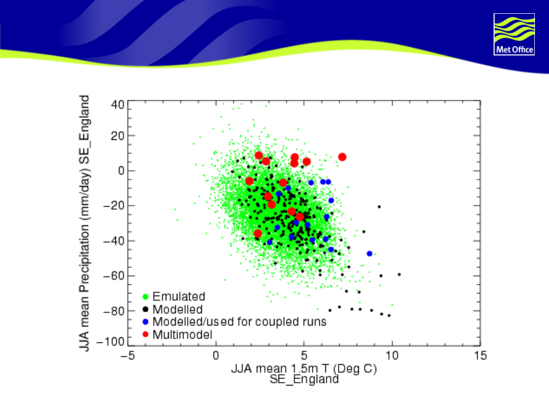
Four types of data…

Page 33

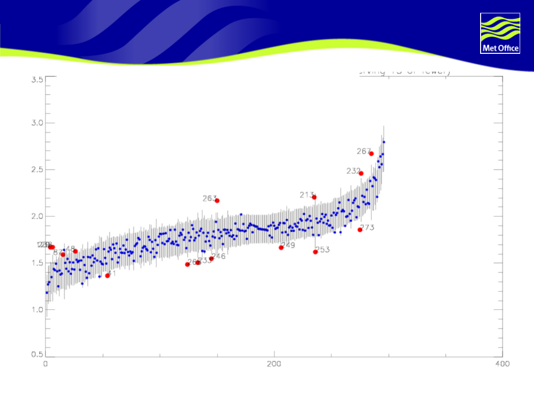
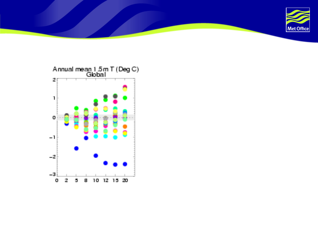
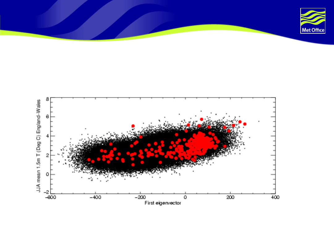
Errors in predicting multimodel
ensemble

•Each dot is a
member of
multimodel ensemble

•Grey shading
represents 95%
confidence interval
from internal climate
variability

A choice: select 10 as this is
as large as possible whilst
still providing a robust
estimate

Number of
observable quantities
in cost function used
to find ‘best input’

Page 34

Climate sensitivity

“Truncation
level” =
amount of
independent
information
from
observations

FOCUS
ON
RED
CURVE

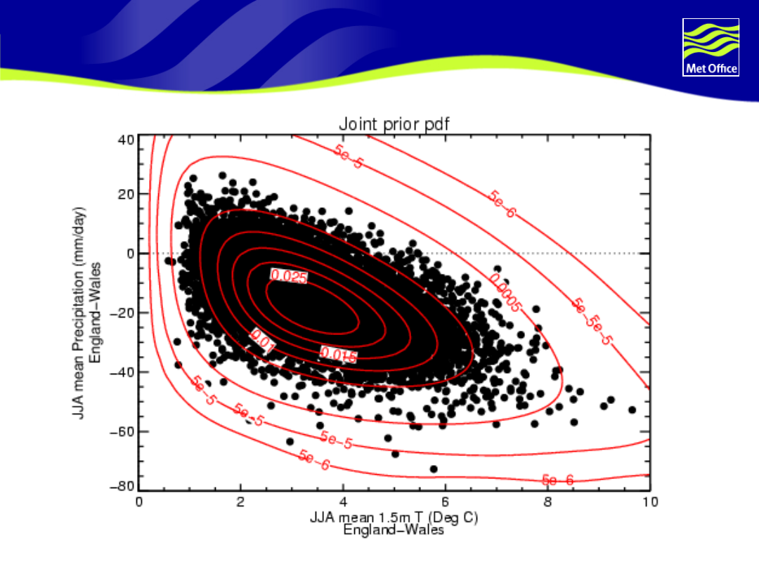
Page 35

Joint probabilities

Page 36

Time scaling

Page 37

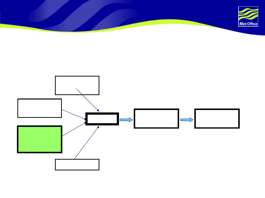
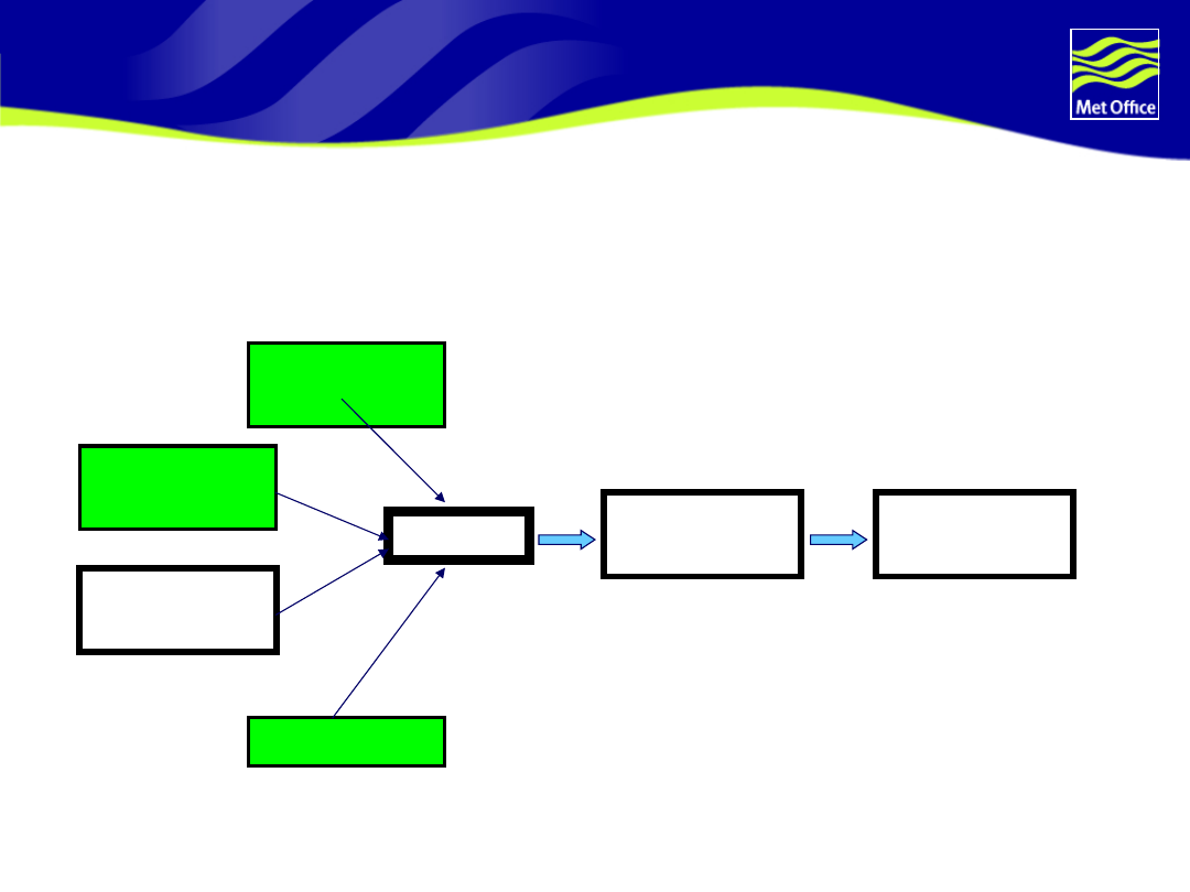
Production of UKCIPnext predictions

EBM

Time-
scaling

Down-
scaling

Equilibrium
PPE

Ocean PPE

Aerosol
PPE

Carbon
cycle PPE

For A1B, B1, A1FI scenarios…

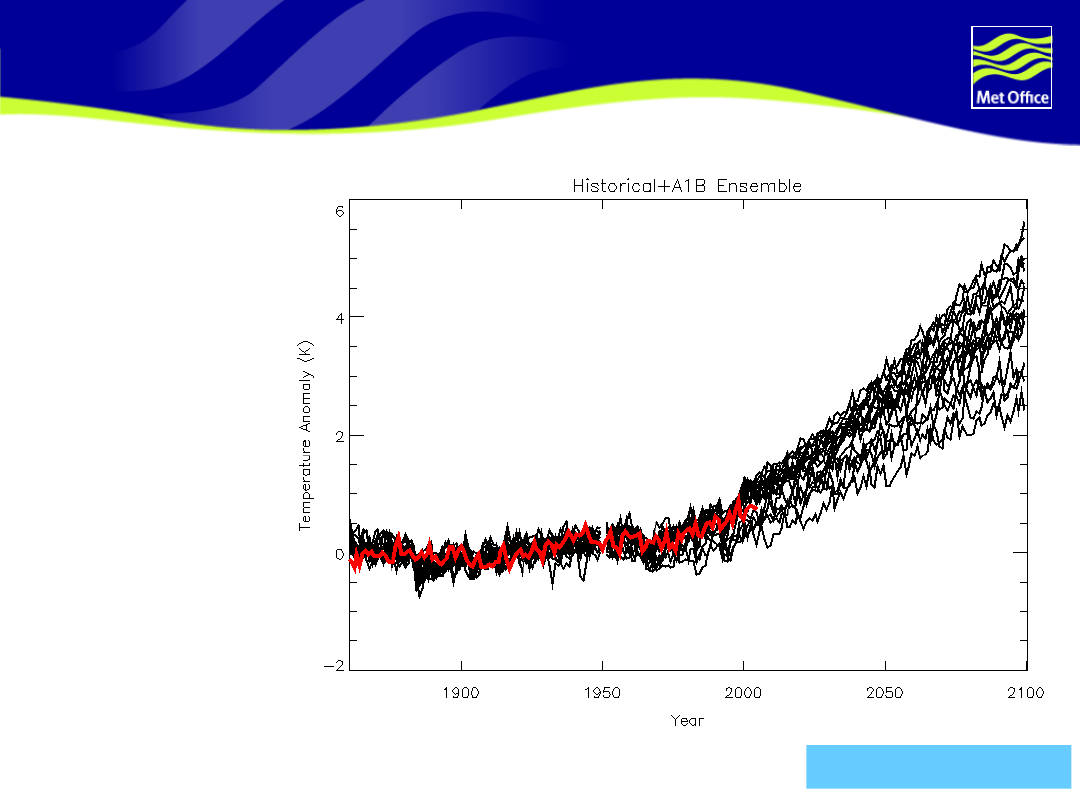
Page 38

Coupled Atmosphere-Ocean
Ensembles

 Smaller

ensembles of
HadCM3
because of
spin-up issues

 Perturbations

to atmosphere-
model
parameters
with equivalent
HadSM3
versions

 Flux

adjustments
used to keep
models stable
and reduce SST
biases

Observations

Historical + A1B

forcing

Collins et al. 2006

Page 39

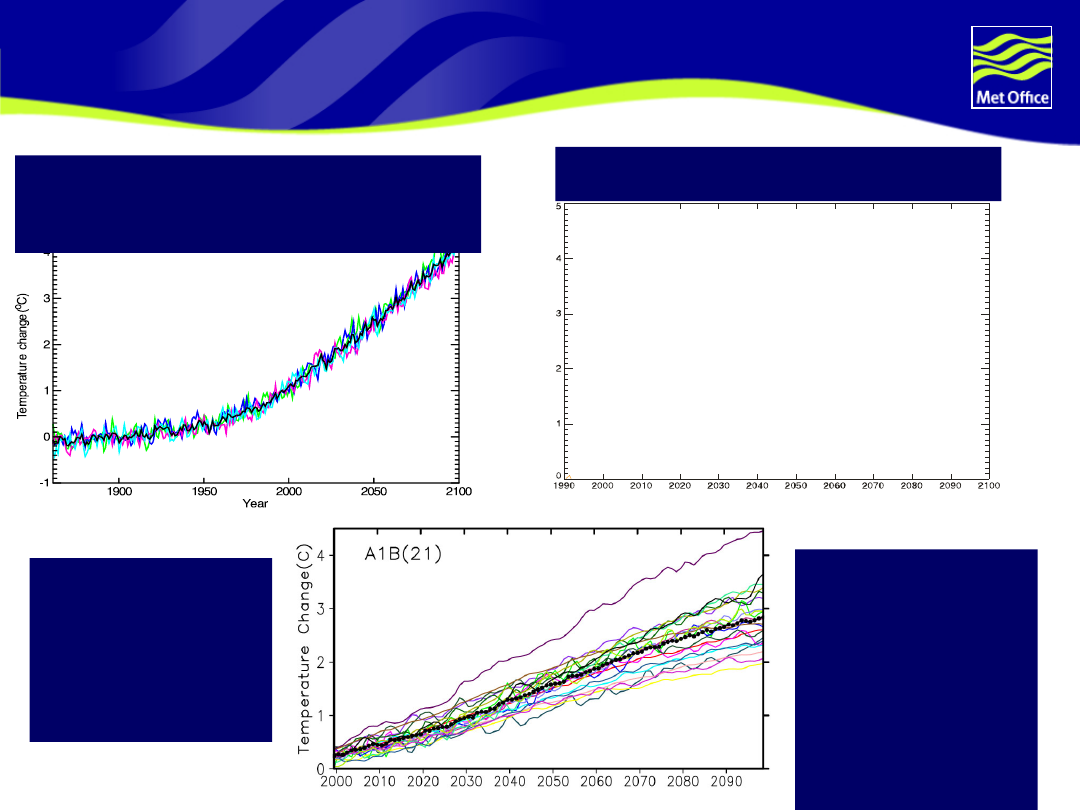
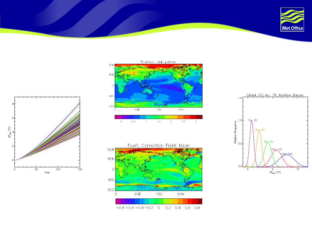
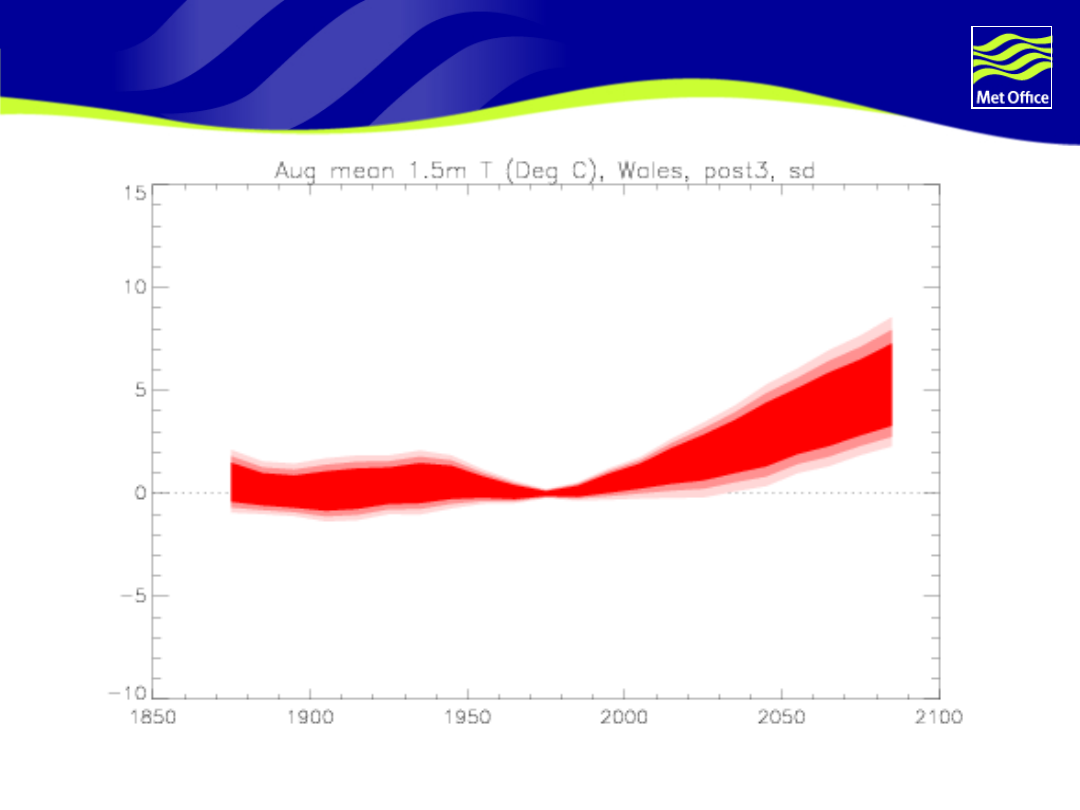
Pattern Scaling to Produce Pseudo-Transient
Ensembles - Methodology







Page 40

Some plumes…Wales August
temperature

No carbon cycle feedback yet

Page 41

Other components

of Earth System

Page 42

Production of UKCIPnext predictions

EBM

Time-
scaling

Down-
scaling

Equilibrium
PPE

Ocean PPE

Aerosol
PPE

Carbon
cycle PPE

For A1B, B1, A1FI scenarios…

Page 43

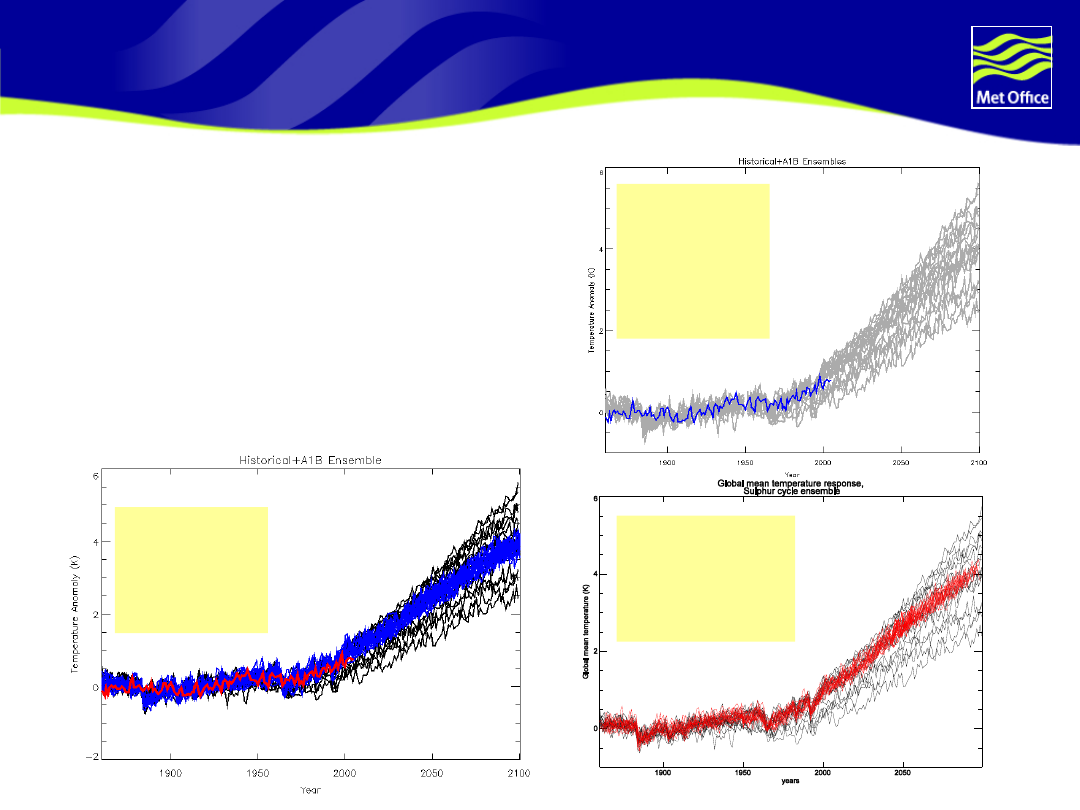
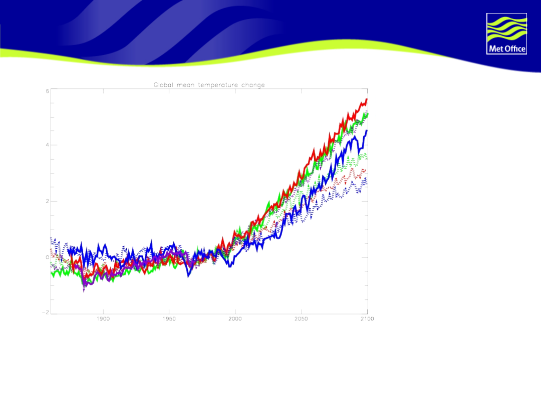
Uncertainties in the transient response of global
mean surface temperature

Ocean
parameter
s
perturbed

Sulphur
Cycle
parameters
perturbed

Atmospher
e
parameter
s
perturbed

Ocean

parameter perturbation

experiments (17 member ensemble)
run to quantify effects of
uncertainties in ocean transport
processes

Sulphur cycle

parameter perturbation

experiments (another 17 member
ensemble) also run

Page 44

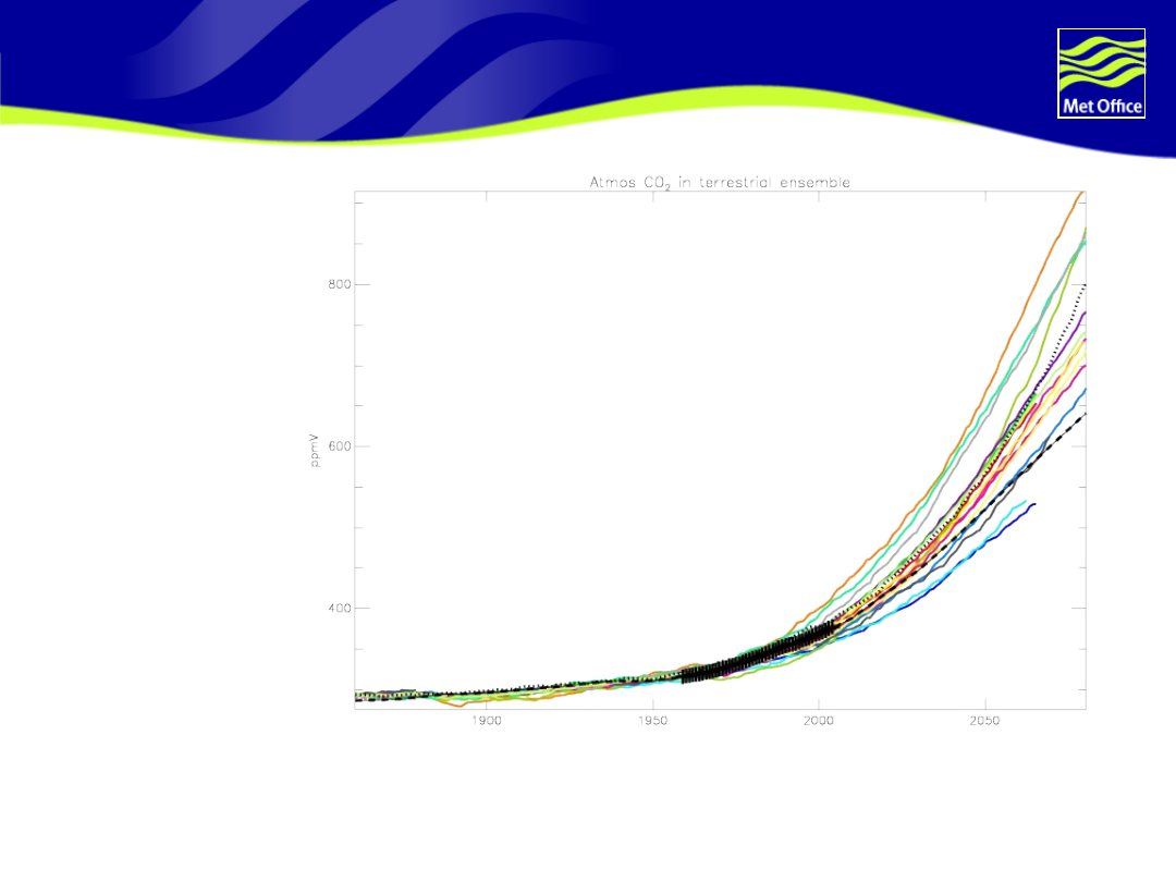
Impact of terrestrial uncertainties on
CO2

Standard HadCM3, 16 variants of terrestrial carbon
cycle

Black crosses - observations

Total
atmospheric
CO2
concentratio
n

Page 45

Downscaling

Page 46

Production of UKCIPnext predictions

EBM

Time-
scaling

Down-
scaling

Equilibrium
PPE

Ocean PPE

Aerosol
PPE

Carbon
cycle PPE

Page 47

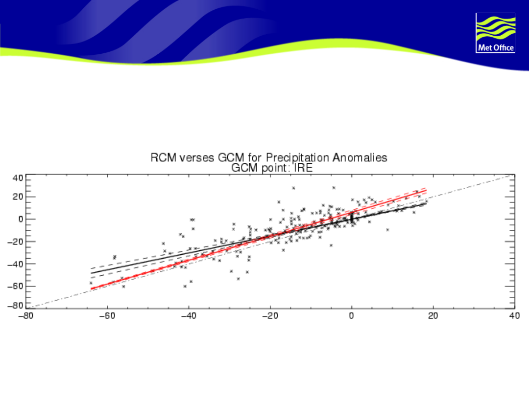
Downscaling

•Have also run a 17-member 25km

resolution ensemble of perturbed
physics regional model versions.

•Driven by boundary forcing from

the HadCM3 A1B transient
simulations (1950-2100).

•We will construct regression

relationships between the 17 GCM
and 17 RCM simulations of future
climate.

•Use these to create regional

response pdfs at 25km scale. Will
add further uncertainty to the
regional responses.

Page 48

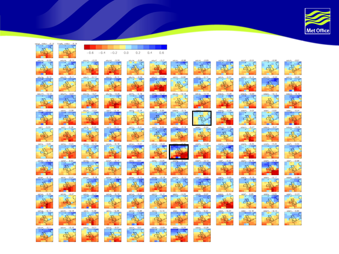
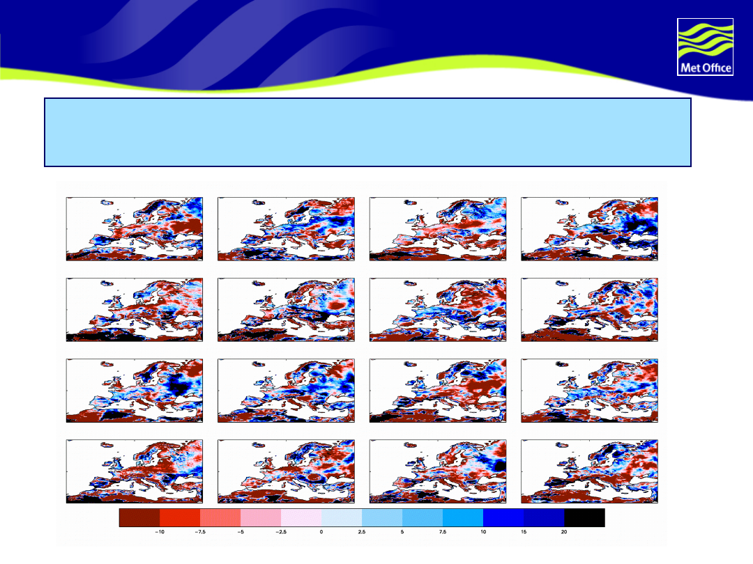
Downscaling uncertainty

16 realisations of the difference in response of the regional model relative
to its driving global model, for January precipitation (% change for 2071-00
relative to 1950-79).

Page 49

Downscaling relationships…

RCM

GCM error

= �

Page 50

Assumptions

Page 51

What are the main assumptions we cannot
test

Local feedbacks between atmosphere

and other components of Earth System

(carbon cycle, aerosol chemistry and

ocean) are of second order importance to

effects linked to global temperature

change.

Structural model uncertainty is a good

proxy for difference between HadCM3

family of models and real system

Pattern scaling, downscaling relationships

applicable across parameter space

Multimodel members have equal

contribution to discrepancy

Page 52

THE END

ANY QUESTIONS?

Page 53

UKCIPnext (Hadley Centre contribution) –
Aims and Objectives

To provide joint probability distribution functions

(pdfs) of predicted changes in a selection of key
UK climate variables at 25km resolution for
each decade during the 21st century

Results will be presented for each variable by

month indicating mainly mean outcomes but
also extremes for e.g. max/min temperature,
precipitation

We aim to deliver the pdfs and final report

summer 2008

Page 54

Sensitivity to prior – climate sensitivity

Before observational After
observational constraint
constraint

Page 55

Sensitivity to prior - %ΔUK summer
rainfall

Before observational After
observational constraint
constraint

Page 56

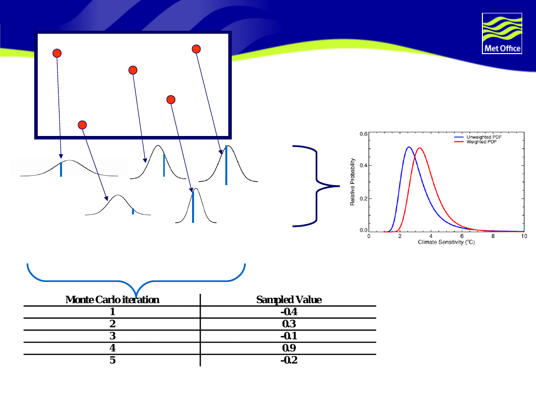
Monte Carlo Sampling

Emulated
Samples

tio

Page 57

Reducing uncertainty

Improve observational uncertainties

Improve model i.e. reduce discrepancy

Run larger ensembles

Use more observational constraints

independent of the ones used already

Remove pattern scaling and downscaling

steps

Remove assumptions about linking sub-

modules

Page 58

Weather Generators

We will make probabilistic predictions for

the variables that are inputted into the

weather generator

Weather Generators will be used to

generate time series consistent with

probabilistic predictions

If need spatially coherent time series at

high temporal and spatial resolution, can

use output from 17 regional climate

model runs

Page 59

Ideal for future UKCIPs

Run 1860-2120 with fully coupled Earth

System Models perturbing parameters in

all components simultaneously and then

downscale

That is, no equilibrium runs, no

ensembles on individual components

Would need other climate centres to run

this experiment for their standard model

and ideally they would have these

downscaled.

Page 60

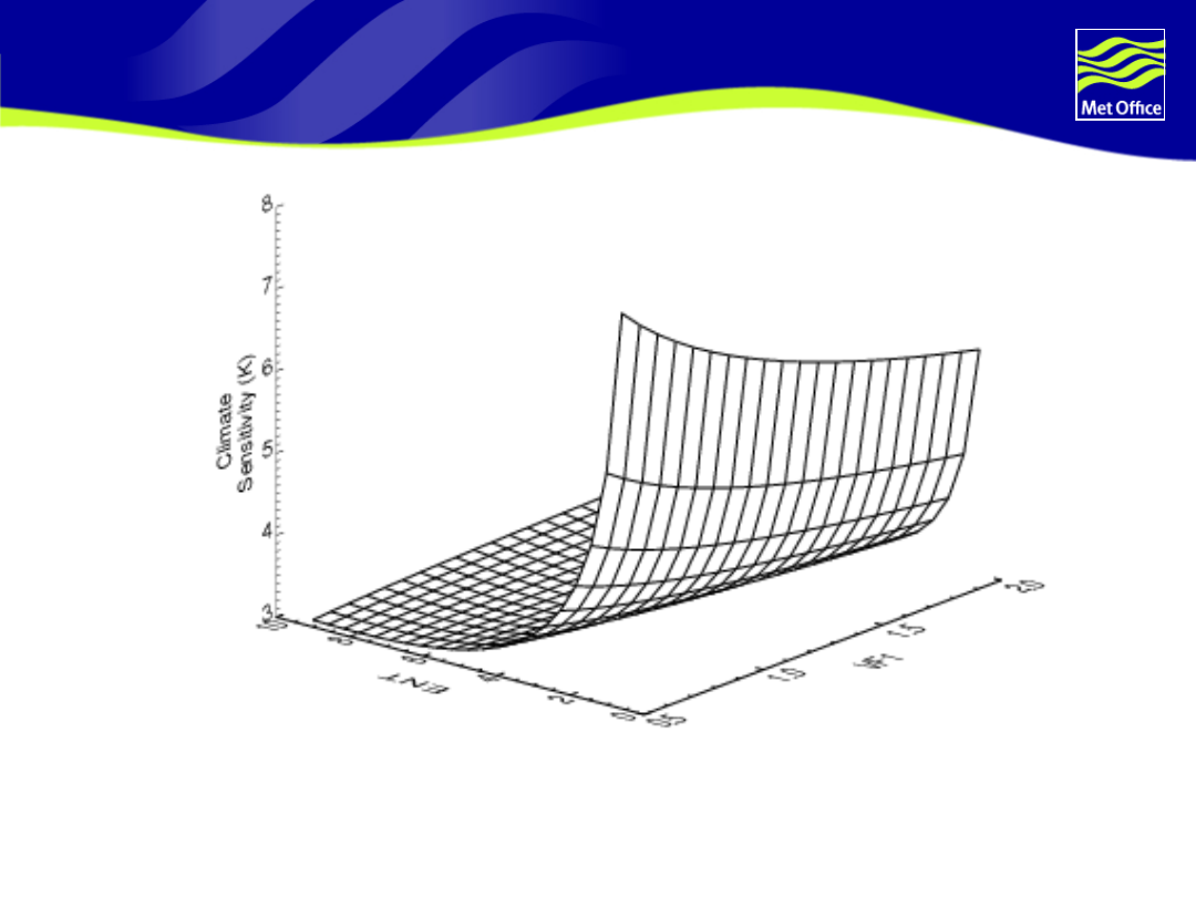
Response surface predicted by
emulator

Climate Sensitivity as a function of two
parameters according to mean prediction of the
emulator – note emulator also predicts
uncertainty of response surface

Page 61

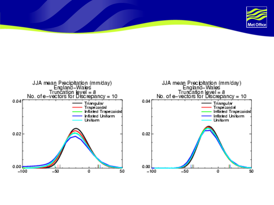
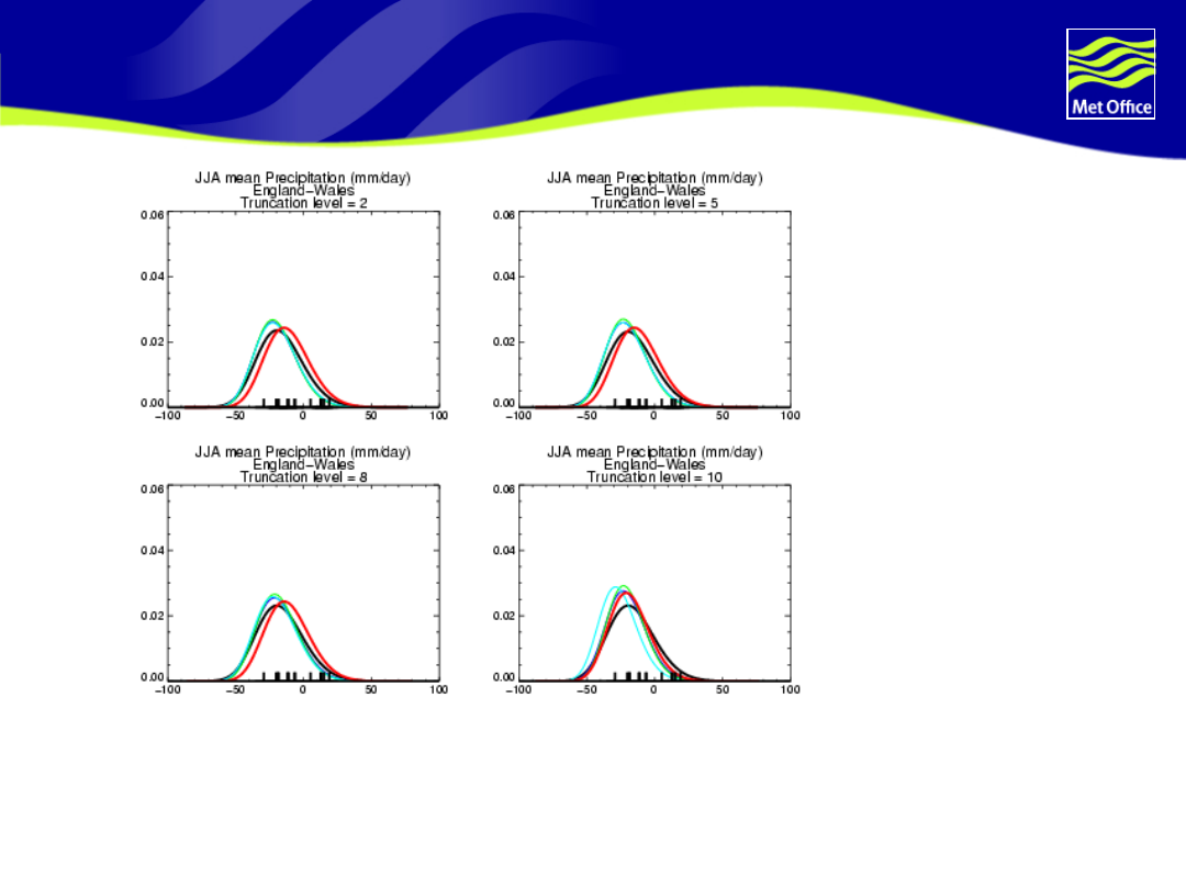
Summer UK % precipitation change

Another choice: what truncation level to choose…

FOCUS
ON
RED
CURVE

Page 62

Probabilistic climate prediction

Probabilistic prediction is a function of

Model
Observations
Choices
Assumptions

Choices guided by principle that we think

it is important to model the Earth System

correctly.

Page 63

Bayesian framework by Goldstein and
Rougier:
some terms

Murphy et al., 2004, Nature, 430,
768-772

histogram of
“perturbed
physics”
ensemble

“emulated”
prior
distribution

posterior
distribution

Page 64

Ensemble Simulations

“Bedrock” provided by a

relatively large ~300
member ensemble of
HadSM3 (atmosphere-slab
ocean) run at 1x and
2xCO

Results sensitive to how

you select parameter
combinations

Murphy et al., 2004
Webb et al., submitted
Stainforth et al., 2005

Page 65

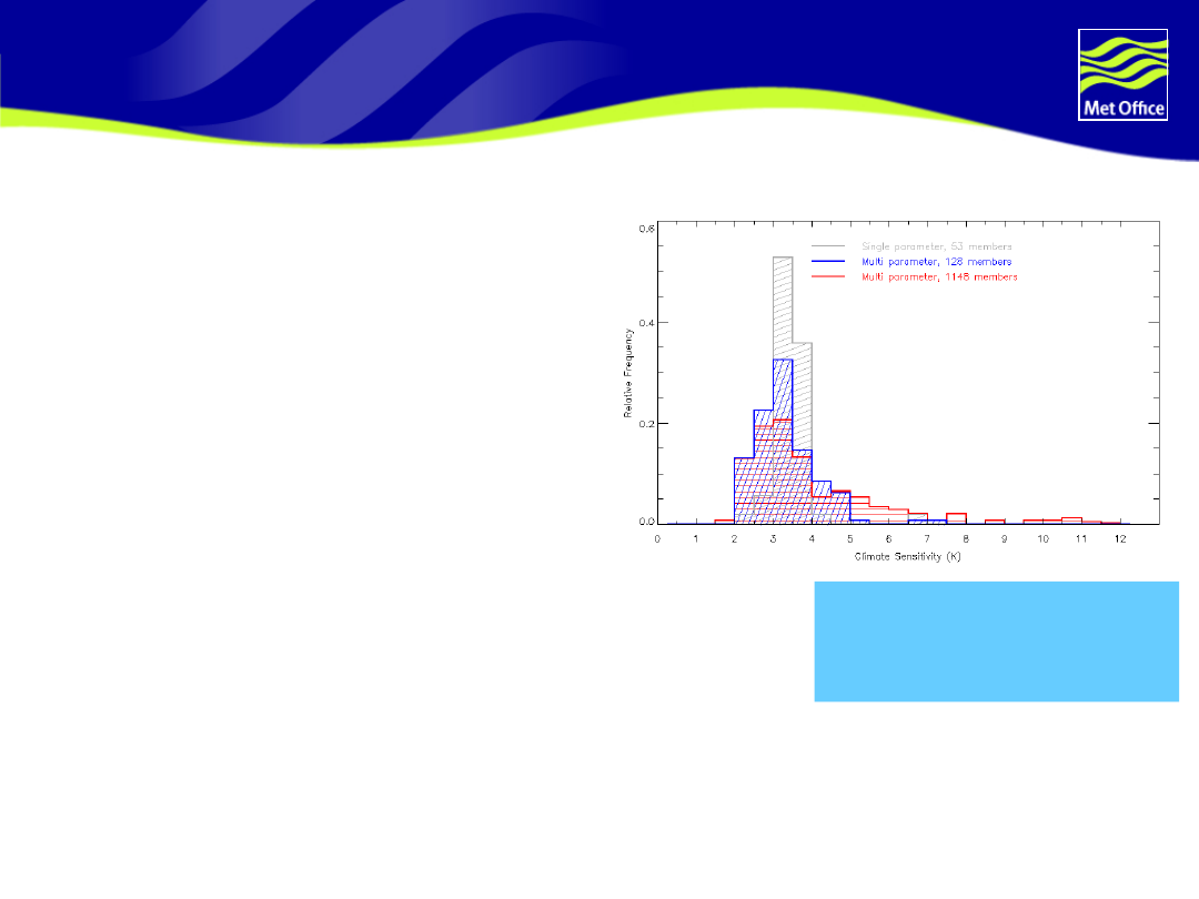
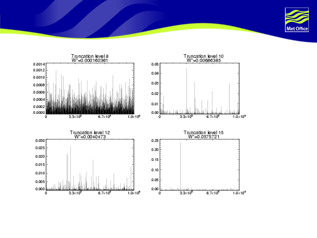
Weights

As truncation level increases, have to be luckier to land on a quality
point in parameter space

Page 66

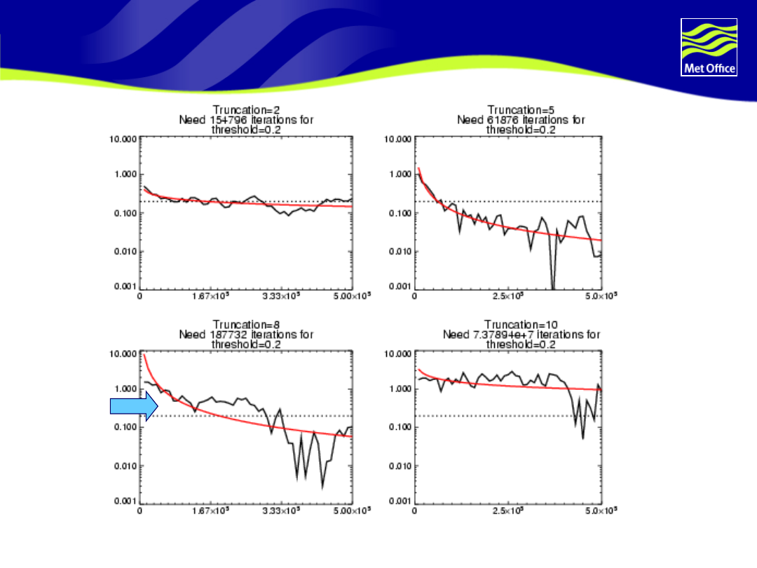
Precision of percentile estimates

Number of Monte Carlo samples 1-0.5
million

Precision
of 95

percentile
estimate

CHOOSE
THIS
ONE!

Page 67

Emulators are statistical models,
trained on ensemble runs, designed
to predict model output at untried
parameter combinations

Emulators

Page 68

Monte Carlo sampling of parameters combined with an
emulator overcomes dependency on sampling strategy to
produce prior prediction (blue line) consistent with beliefs about
where the best input lies.

Prior distribution

– prediction before any observations used

Emulators and priors