Comparing Passive and Active Worm Defenses

∗

Michael Liljenstam

University of Illinois at Urbana-Champaign

Coordinated Science Laboratory

1308 W Main St.

Urbana, IL 61801

mili@crhc.uiuc.edu

David M. Nicol

University of Illinois at Urbana-Champaign

Coordinated Science Laboratory

1308 W Main St.

Urbana, IL 61801

nicol@crhc.uiuc.edu

Abstract

Recent large-scale and rapidly evolving worm epi-

demics have led to interest in automated defensive mea-
sures against self-propagating network worms. We
present models of network worm propagation and de-
fenses that permit us to compare the effectiveness of
“passive” measures, attempting to block or slow down a
worm, with “active” measures, that attempt to proac-
tively patch hosts or remove infections. We extend
relatively simple deterministic epidemic models to in-
clude connectivity of the underlying infrastructure,
thus permitting us to model quarantining defenses de-
ployed either in customer networks or towards the
core of the Internet. We compare defensive strate-
gies in terms of their effectiveness in preventing worm
infections and find that with sufficient deployment, con-
tent based quarantining defenses are more effective than
the counter-worms we consider. For less ideal deploy-
ment or blocking based on addresses, a counter-worm
can be more effective if released quickly and aggres-
sively enough. However, active measures (such as
counter-worms) also have other technical issues, includ-
ing causing additional network traffic and increased risk
of failures, that need to be considered.

∗

This research was supported in part by DARPA Contract
N66001-96-C-8530, NSF Grant CCR-0209144, and Award No.
2000-DT-CX-K001 from the Office for Domestic Preparedness,
U.S. Department of Homeland Security. Points of view in this
document are those of the author(s) and do not necessarily rep-
resent the official position of the U.S. Department of Homeland
Security.

1. Introduction

The proliferation of large-scale malware attacks in

recent years has brought high costs for clean up, data
loss in some cases, and much nuisance to users. Self-
propagating worms—such as Code Red v2 [12, 18],
Code Red II [18], Nimda [18], and more recently Slam-
mer [11] and Blaster [17]—have attracted particular
attention for their demonstrated potential to spread
across the Internet in a matter of hours or even min-
utes. Defending against such a rapid attack is thus
fundamentally harder than responding to most email
borne malware where the requirement for a user to per-
form some action (e.g. opening an attachment) slows
it down. Hence, the rapid spread potential has spurred
significant interest in models to understand the dynam-
ics of self-propagating worm spread and investigate the
feasibility of worm detection and defense capabilities.

We model and compare the mean performance of a

few different proposed defensive techniques, in terms
of their ability to prevent worm infections. In particu-
lar, we compare what we call “passive measures” that
try to block worm traffic to prevent spread with what
we call “active measures” that try to proactively patch
vulnerable hosts or remove infections from hosts in re-
sponse to an attack.

A necessary prerequisite for any response is quick

and accurate detection. Beyond that, the effective-
ness depends on the strategy chosen. Passive measures,
such as host quarantining, pose an intuitively appeal-
ing strategy for stopping, or at least slowing down,
the spread of a worm. But to be effective they require
widespread deployment in the Internet. More drastic
(“active”) measures, such as launching a second worm
that tries to patch vulnerable hosts to prevent infec-
tion or remove the first worm from infected systems,
do not require infrastructure to be in place. However,

active measures have many legal, ethical, and techni-
cal issues that may prevent them from being used:

•

Breaking into someone else’s machine, even if it is
to fix a vulnerability, is illegal.

•

Patches sometimes contain bugs or unexpected
sideeffects,

systems

administrators

typi-

cally want them to be tested first rather than
forced onto the machines by someone else.

•

Launching a second worm leads to more scan-
ning traffic and consequently more consumption
of network resources, which can exacerbate net-
work problems from the original worm.

Nevertheless, worms that attempt to patch against or
remove another worm have actually been seen in the
wild, as in the case of the Welchia worm [5] removing
Blaster. Whether Welchia was intended as a counter-
worm or merely another worm “feeding off” the first
one, there was evidence of Welchia causing at least as
much of a problem as Blaster. Consequently, it is rea-
sonable to ask if such an approach could be viable from
a strictly technical standpoint, and how it compares to
other strategies in terms of effectiveness.

In a previous study [15] we examined several active

measures and compared them in terms of their effec-
tiveness at preventing host infections and their impact
on the network (additional traffic induced). Here, we
present models of passive defenses and compare active
measures against passive measures. We will not con-
sider network impact, but instead refer to [15] for a
discussion and note that this is also an important di-
mension in making a comparison. Since active measures
are associated with several issues, we assume that they
are only launched as a last resort when an attack has
been detected, and never “proactively” ahead of time.

The first step for examining defenses is to under-

stand the worm propagation dynamics. Worms, such as
Code Red v2, that spread by probing addresses in the
address space with uniform probability are particularly
simple to model because of the “homogeneous mix-
ing” of infectives and susceptibles. This corresponds
well with assumptions in many epidemic models [4].
Self-propagating worms have been modeled using con-
tinuous time deterministic models (simple epidemics)
[18, 12, 9], discrete time deterministic models [2],
stochastic simulations [13, 9, 25, 20], and stochastic
models for malware spread over networks [8]. Some
worm models have been extended to other scanning
strategies [2, 23] or have been used to study defense
systems [13, 2, 15]. Competition between two kinds
of malware was studied in [19] using a predator-prey
model. Our study has most in common with the study
by Moore et al. [13], where they studied the feasibility

of quarantine-based worm defenses. They used stochas-
tic simulations and studied both content filtering and
address blacklisting based methods. They found con-
tent filtering to be more effective than address black-
listing. However, content filtering, unlike address black-
listing, is not readily implementable with current tech-
nology; and in any case they concluded that the avail-
able response time to contain quickly spreading worms
is so small that there appears to be little hope for suc-
cess. We also study these types of defenses, using sim-
ilar assumptions but simpler models, and we contrast
them with active defense measures.

We present simple models, based on epidemic mod-

els, for several defense strategies that take network con-
nectivity into account and thus permit us to compare
active and passive defenses while varying deployment.
Results from numerical solutions indicate that passive
defenses based on content filtering can protect more
hosts from infection than the active defenses we con-
sider here, given fairly extensive deployment in the In-
ternet. If that level of deployment cannot be achieved,
or content filtering cannot be done reliably, then active
defenses might protect more hosts if the response can
be done quickly and aggressively. However, this would
come at the price of additional scanning traffic and the
possibility of problems resulting from counter-worm in-
fections. By using relatively simple epidemic models,
we are also able to derive an analytic result regard-
ing the performance of a patching worm versus a con-
tent filtering system deployed in customer networks.

The remainder of this paper is organized as follows.

Models for each defensive strategy are presented in Sec-
tion 2 with examples and characterization of perfor-
mance. Section 3 then proceeds to compare blocking
(passive) defenses deployed in customer networks, i.e.
towards the “edge” of the Internet, with active mea-
sures. In Section 4 we consider the case where passive
defenses can be deployed in highly connected networks
in the “core” of the Internet and compare this case with
active measures. Conclusions are given in Section 5.

2. Models

Triggered by recent attention on large-scale malware

spread there has been a flurry of studies using models
of epidemic spreading over graphs [8, 22, 16, 14] typ-
ically with the assumption that the infection spreads
between neighboring nodes in the graph (such as social
graphs where email viruses spread through the email
contact network).

Our goal is different since we want to model the

effects of the underlying network (the Internet) for
actively spreading network worms. Thus, we model

worms that spread by random scanning, such as the
Code Red v2 (July, 2001) and Slammer (Jan., 2003)
worms, and we include network topology to model the
effects of defensive measures deployed in the network
or effects on the network infrastructure itself. Note that
the topology of the “worm spread network” (where the
worm is spreading from neighbor to neighbor) will thus
be very different from the topology of the underlying
infrastructure (Internet topology) and there is no rea-
son to expect it to resemble scale-free graphs or small
world models, as frequently studied recently. We will
discuss this some more in Sections 2.1 and 4.1.

As our starting point, we use the stratified simple

epidemic model [4], a well known model from the epi-
demic modeling literature. In this model we consider a
fixed population of N , where each individual is either
in state S (susceptible to infection) or I (infected). We
denote by s

(t) and i

(t) the number of individuals in

state S and I respectively at time t in population stra-
tum j. Thus, ∀t,

(t)+i

(t) = N . For large enough

populations, the mean rate of state changes S → I can
be modeled as:

(t)

= −s

(t)

= s

(t)

where β

is the infection parameter, i.e. the pairwise

rate of infection, from network k to network j. The sys-
tem boundary conditions are given by the number of
initially susceptible hosts s

(0) and initially infected

hosts i

(0). This model rests on assumptions of homo-

geneous mixing, which correspond well to a uniformly
random scanning worm spreading freely through a net-
work. Consequently, this type of relatively simple epi-
demic models have been used successfully [18, 12, 9] to
describe the growth dynamics of network worms, such
as Code Red v2, that spread by uniform random scan-
ning.

We model connectivity in the network the worm is

spreading over by considering K separate subnetworks,
the “strata” in our model. These could be, e.g., Au-
tonomous Systems or smaller networks. The K × K
connectivity matrix C(t) has element c

= 1 if net-

work j can send worm scan traffic to network i at time
t

, otherwise c

= 0. The populations of penetrated (in-

fected) hosts is described by the K × 1 column vector
P

(t), such that p

(t) = i

(t), and the populations of vul-

nerable (susceptible) hosts in K × K matrix V (t), with
diagonal elements v

(t) = s

(t).

We let ∀i, j β

= β,

Since I generally refers to the identity matrix we want to avoid

i.e., all infection parameters are the same, and uncon-
strained infection growth under connectivity is then

(t)

= βV (t)C(t)P (t)

Under normal operation, the connectivity matrix C

would typically be all ones, meaning that scans can
pass between all networks in the Internet. We call this
the unconstrained random scanning model. Note,
that for the case of full connectivity it is possible to sim-
plify the model into a homogeneous epidemic model [4].
However, it has been observed that the intense scan-
ning traffic might affect the network infrastructure to
induce failures at some points in the network [3], which
would affect connectivity in the network. Moreover, we
next look at models of some defensive measures that
can block scans from traversing the network, and thus
affect C(t).

Note that this model describes the mean evolution

of the system. In [13], Moore et al. note that when at-
tempting to predict the effectiveness of a defensive sys-
tem, it is preferable to consider the quantiles of infec-
tion rather than the mean number of infections due
to the variability inherent in the early stages of infec-
tion growth. However, we are mainly concerned with
the relative performance of different defenses as we
compare them, and we believe that the relative per-
formance can be credibly determined in terms of the
mean, even though the predicted mean absolute per-
formance should be viewed with caution. Moreover, the
relative simplicity of these models sometimes permit us
to do some analysis, which is not possible with stochas-
tic simulations (as needed to estimate quantiles).

2.1. Content Filtering

Defenses based on content filtering suppose that

worm packets have discernible signatures. They dis-
cover and disseminate these signatures to a distributed
infrastructure that filters traffic to eliminate discov-
ered worm packets. Success of these defenses depend
on very fast response to an attack, and a filtering in-
frastructure that protects a large fraction of the net-
work.

We can model the content filtering defense in the

network as follows. Before content filtering is invoked,
the system evolves according to the unconstrained ran-
dom scanning model. The defense system is then in-
voked at time T

. Thus, at T

, C(t) changes to reduce

the connectivity for worm scanning traffic. How much
connectivity is reduced depends on where the defenses

it as we define our notation here. We also avoid S since we have
used it to denote a state. Hence, the name changes.

are deployed in the network and to what extend de-
ployment is carried out.

Customer deployment: For quarantining de-

ployed in customer networks, we assume that it is de-
ployed very close to the hosts, so that it effectively
blocks a certain fraction of all hosts in the Inter-
net, leaving other hosts still open. Let p be the prob-
ability of encountering an unprotected host, i.e. an
open path. We can model this scenario in a sim-
ple fashion by conceptually grouping together all hosts
into two networks: (1 − p)N protected hosts in net-
work 1, and pN unprotected hosts in network 2.
Hence, we have K = 2, and for t > T

(t) =

0 0
0 1

meaning that infection can only spread among unpro-
tected hosts. Note that this means that the “worm
spread network” topology described by C(t) in this sce-
nario is still simply a clique involving all the unpro-
tected hosts. Another minor note is that the boundary
conditions now need to include whether the initially in-
fected hosts i(0) belong to the protected set or not. In
the following we will assume that they are unprotected.

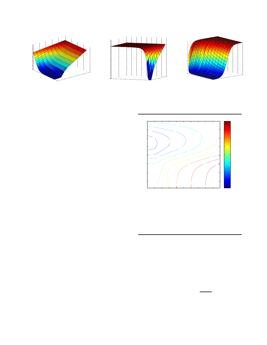
The number of infections after a certain time T gives

us a way of comparing the effectiveness of defenses in
different situations. For instance, the left graph in Fig-
ure 1 shows the number of infected hosts after 24 hours
as a function of response time T

and the probability of

an open path p using Code Red v2 parameters for worm
spread. For this example and the remainder of the
paper we used worm propagation parameters for the
Code Red v2 worm from [9] to illustrate and make com-
parisons: we assume N = 380000, β = 5.65 · 3600 · 2

and that the infection starts from a single host. Note
that the dynamics are qualitatively the same for worms
that spread faster or slower or with a different suscepti-
ble population, as long as the propagation strategy re-
mains the same (uniform random scanning) and there
is not significant network congestion resulting from the
worm. Although some other propagation strategies can
also be modeled using similar techniques, it is beyond
the scope of this study. Not surprisingly, the extent
of deployment is a crucial factor as it determines how
many hosts are protected. With deployment covering
90% or more of the hosts, the defense could be effec-
tive in terms of the mean number of infections it pre-
vents for response times up to 4 or 5 hours. However,
quickly spreading worms, such as Slammer, could re-
duce the available response time to the order of min-
utes or less, making it very difficult to counter it in
time.

Core deployment: For quarantining deployed in

the core of the Internet we compute the connectivity
C

(t), t > T

from a network graph. We discuss this in

more detail later, in Section 4, where we compare dif-
ferent defensive measures.

2.2. Address Blacklisting

Another defense is based on blocking traffic from

certain specific IP addresses (address blacklisting) that
are known or suspected to be infected by the worm.
In this case it seems plausible that there will be two
kinds of response times: the first T

is the time to de-

tect that there is an attack in progress, and the sec-
ond T

is the time to detect that a specific host is or

might be infected. The reason for making a distinction
is that it seems likely that in general T

> T

. Once it

has been established that a, possibly global, attack is
in progress it is likely to be easier to detect suspected
infectives. For simplicity we will assume a single re-
sponse time parameter here T

= T

, since this

also makes it easier to compare results with [13] where
this distinction was not made. Thus, the response time
T

denotes the time from when a specific host is in-

fected by the worm until that information has been
disseminated to all parts of the system so that traf-
fic from the host can be blocked.

Address blacklisting can be modeled as follows. We

split the infected populations P (t) into detected and
undetected subpopulations P

(t) and P

(t). At time

, the time of first response, the initial infections

(0) are detected and are assigned to P

). All in-

fections on [0, T

] are as yet undetected so P

) con-

tains P (T

)−P (0) infections. Define the new infections

at t, for t ≥ T

, to be

new

(t) = β[V (t)C

(t)P

(t) + V (t)C(t)P

(t)]

where C

(t) is the unprotected connectivity matrix, i.e.

with all entries being ones. The first term describes how
undetected worms can interact unhindered with any
susceptible and the second term describes how some
detected worms are blocked by the system. The transi-
tions into infections are described by the delay differ-
ential equations

(t)

= P

new

(t) − P

new

(t − T

)

(t)

= P

new

(t − T

)

Defense deployment in customer networks and In-

ternet core networks can be modeled in the same way
as for content filtering mentioned earlier. This method
tends to be less effective than content filtering due to
the delay in detecting every new infected host. Because

of the relationship between T

, the infection rate, and

the initial worm population, the system tends to ini-
tially lag behind in detecting new infections and only
catches up once the infection slows down. Effective-
ness as a function of response time and customer net-
work deployment is shown in the middle graph of Fig-
ure 1. It is evident from this graph that for this de-
fense to be effective it is crucial to make the response
time delay small.

2.3. Patching Counter-Worm

In [15] we studied and compared several “active”

worm countermeasures where, rather than just block-
ing worm scans, an attempt is made to actively inhibit
the spreading worm. For instance, through proactive
patching of hosts, or by attempting to gain entry into
infected hosts and removing the worm. Our motivation
for studying this type of defenses stem directly from at-
tempts that have been made to launch worms that re-
move other worms from a system, e.g. as Welchia tried
to remove Blaster [5] and install a patch to fix the vul-
nerability.

Consider a counter-worm that is launched in re-

sponse to an attack, uses the same vulnerability and
propagation strategy as the original worm, but is un-
able to enter hosts that have already been taken over
by the original worm. As the counter-worm enters the
host it will take measures to protect the host from fur-
ther infection, preferably by installing a patch that re-
moves the vulnerability. Under these assumptions the
second worm will spread at (approximately) the same
rate as the original worm, seeking the same suscepti-
ble population of hosts. A simple model is:

(t)

= −βV (t)C(t)(P

(t) + P

(t))

(1)

(t)

= βV (t)C(t)P

(t)

(2)

(t)

= βV (t)C(t)P

(t)

(3)

where P

refers to infections by the malicious (bad)

worm and P

refers to infections by the patching (good)

worm. We call this the Patching Worm Model.
Given β and P

(0), system behavior is governed by

the time T

at which patching worms are released, and

the number of patching worms I

P P

) released.

We assume that the patching worms are launched on
“friendly” machines that are not part of the suscepti-
ble or infected set, and that they spread using the same
mechanism (thus same β).

We will assume that the counter-worm spreads un-

der full connectivity, i.e. C

(t) = 1 ∀i, j unless stated

otherwise. Patching worm effectiveness as a function

of response time and initial population is shown in the
right-hand graph of Figure 1 for unconstrained connec-
tivity. An effective response requires a combination of
low response time and a sufficiently large initial pop-
ulation. Launching a single counter-worm has little ef-
fect, and the window of opportunity for launching even
a thousand patching worms disappears after a couple
of hours in the Code Red scenario.

2.4. Nullifying Counter-Worm

We call a counter-worm able to identify an infected

host and suppress its scanning a nullifying worm. We
may distinguish between two types of nullifying worms.
One model of nullifying worms assumes that they can
only suppress an infected host, not gain it as another
platform, call this a “type-1” nullifying worm. Such
a capability would depend on an ability to intercept
and filter the scans near their source, like a dynamic
IP-address filtering capability that is erected where
worms are discovered (similar to quarantining). The
“type-2” version assumes an infected host can be en-
tered, the infection removed, and the nullifying worm
installed. In [15] we considered properties of the type-1
counter-worm. Here we will focus on the type-2 counter
worm, which resembles worms seen in the wild, such
as Welchia [5]. One should note, however, that intrud-
ers have been known to patch the vulnerability used
to gain entry to a system to prevent others from sub-
sequently gaining entry; and a worm could similarly
block a nullifying worm by preventing later exploita-
tion of the same vulnerability. Nevertheless, since this
technique has been used in practice we will consider it
here.

State equations for the type-2 counter-worm can be

written as the Nullifying Worm Model:

(t)

= −βV (t)C(t) [P

(t) + P

(t)]

(t)

= β

V (t)C(t)P

(t) − P

(t)C(t)P

(t)

= β

V (t)C(t)P

(t) + P

(t)C(t)P

(t)

where P

(t) and P

(t) are K × K matrices with diag-

onal elements p

= p

from the corresponding column

vector.

In [15] we showed that a nullifying worm system

is more powerful than a patching worm, in the sense
that given identical initial conditions, the size of the in-
fected population at any instant in time is larger in a
patching worm context than in a nullifying worm con-
text.

Given sufficient time, the nullifying worm will erad-

icate the original worm. However, hosts that have at

0.2

0.4

0.6

0.8

100

120

Probability of open path

Response time [h]

% hosts infected after 24 hrs

0.5

100

120

Probability of open path

Response time [h]

% hosts infected after 24 hrs

200

400

600

800

1000

100

Response Time (T

) [h]

Response Population (I

)

% hosts infected by malicious worm

Figure 1. Effectiveness of: LEFT—content filtering as a function of response time and deployment, CENTER—
address blacklisting as a function of response time and deployment, RIGHT—patching worm as a function of re-
sponse time and initial counter-worm population.

some point been infected by the original worm may suf-
fer ill effects from the intrusion (such as data destruc-
tion, implanted trojans or back-doors), so in our com-
parisons we will focus on the number of hosts “touched”
by the original worm.

3. Comparison: Edge Deployed Passive

Defenses

In this section we compare passive defenses (con-

tainment) deployed in customer networks, i.e., at the
“edge” of the network, with active defenses.

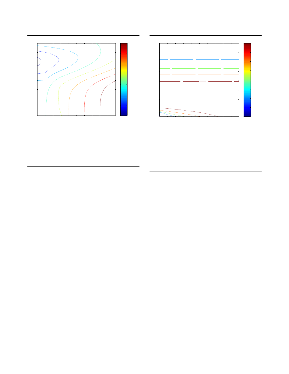
3.1. Comparison with Patching Worm

For a direct comparison of the effectiveness of the ac-

tive defenses we have described here with containment
strategies, we vary response time and containment de-
ployment and fix the remaining active defense parame-
ter. We first consider the patching worm. Figures 2 and
3 compare the patching worm, using an initial response
population I

= 1000 hosts, with content filtering and

address blacklisting, respectively. These are contour
plots of the infection percentage for containment mi-
nus bad worm infection percentage while countering
with a patching worm. Consequently, a negative per-
centage means that the containment system resulted in
fewer infections. The graphs indicate that content fil-
tering is more effective than a patching worm when it
can protect at least 86% of the hosts, and for later re-
sponses the patching worm is quite ineffective so con-
tainment wins also for lower coverage. Address black-
listing, on the other hand, is more effective only for
very short response delays and near perfect coverage.
Thus, there appears to be realistic situations where a
patching worm could protect more hosts from infection
than an address blacklisting defense, at the cost of re-
maining high bandwidth usage. As the response time

0.1

0.2

0.3

0.4

0.5

0.6

0.7

0.8

0.9

Probability of open path

Response Time [h]

Comparison I

=1000

−80

−60

−40

−20

−80

−60

−40

−20

Figure 2. Direct comparison between content fil-
tering and patching worm. Percent infections us-
ing content filtering minus infections when em-
ploying patching worm. When positive, counter-
worm is better. Counter-worm is launched with
initial population I

= 1000 hosts.

increases, both approaches are ineffective and the dif-
ference diminishes.

With the counter worm spreading under full con-

nectivity, we can simplify equations 1–3, by letting
s

(t) =

P V (t), i

(t) =

P P

(t), i

(t) =

P P

(t), and

removing C(t). In [15] we showed that under these con-
ditions, the fraction of hosts ultimately protected by
the patching worm (i.e. as t → ∞) is

patching

= ρ

1 −

)

(0)

where ρ is the counter worm response population frac-
tion. That is, if the number of counter worms released

0.1

0.2

0.3

0.4

0.5

0.6

0.7

0.8

0.9

Probability of open path

Response Time [h]

Comparison I

=1000

Figure 3. Direct comparison between address
blacklisting and patching worm. Percent infec-
tions using content filtering minus infections
when employing patching worm. When posi-
tive, counter-worm is better. Counter-worm is
launched with initial population I

= 1000 hosts.

at time T

is I

, then

+ i

)

Using the same notation, the fraction of hosts pro-
tected by customer deployed content filtering (again
as t → ∞) is

cont.f.

= (1 − p)

)

where p is the probability of encountering an unpro-
tected host, as before. That is, ˜

cont.f.

will be the

fraction of protected susceptible hosts remaining when
content filtering is invoked. Comparing ˜

patching

with

cont.f.

leads to the following analytical result:

Theorem 1 (Content filtering vs. patching
worm). Assume a patching counter worm, spread-
ing at the same rate as the original worm, is released at
I

hosts with response time T

; and assume the same re-

sponse time for customer deployed content filtering
protecting a fraction 1 − p of the hosts. A patch-
ing counter worm, on average, protects at least as many
hosts as customer deployed content filtering iff the frac-
tion of hosts left open by the content filtering system
is

p ≥

1 −

(N − i

))(I

+ i

))

1 −

)

(0)

where it is known that

) =

(0)N

(0) + (N − i(0))e

−βN T

Proof. The patching worm is better iff the protected
fraction for content filtering is less, i.e. ˜

cont.f.

≤

patching

. Consequently, when

(1 − p)

)

≤

1 −

)

(0)

rearranging

p ≥

1 −

ρN

)

1 −

)

(0)

For 0 ≤ t ≤ T

we have a single worm spreading and

the invariant N = s(t) + i

(t). Hence,

) = N − i

)

substituting this in, and expanding ρ gives us

p ≥

1 −

(N − i

))(I

+ i

))

1 −

)

(0)

And i

) follows immediately from the known closed

form solution to the simple epidemic model [4] we have
for the single worm spreading up to time T

Quantities such as i

) and s(T

) can likely be es-

timated from observed scanning behavior [24]. Thus,
this result could aid in the choice of a counter mea-
sure once an attack is detected.

3.2. Comparison with Nullifying Worm

Next consider a similar comparison for the hosts

touched by the bad worm while countering with a nul-
lifying worm, as shown in Figures 4 and 5. The nullify-
ing worm is slightly more effective as it also slows down
the propagation of the bad worm. Content filtering now
requires approximately 89% coverage to provide better
protection for quick responses and it outperforms ad-
dress blacklisting in all cases. However, this still comes
at the price of scanning bandwidth usage and worm in-
fections.

4. Comparison: Core Deployed Passive

Defenses

In this section we consider the case where the quar-

antining (passive defense) system is deployed in highly
connected ISPs in the core of the Internet. The per-
formance of core deployed content filtering was consid-
ered by Moore et al. [13]. We model, using differential
equations, both content filtering and address blacklist-
ing deployed at the Internet core and compare with
counter-worms.

0.1

0.2

0.3

0.4

0.5

0.6

0.7

0.8

0.9

Probability of open path

Response Time [h]

Comparison I

=1000

−60

−40

−20

−60

−40

−20

Figure 4. Direct comparison between content
filtering and nullifying worm. Percent infec-
tions using content filtering minus hosts touched
when employing nullifying worm. When posi-
tive, counter-worm is better. Counter-worm is
launched with initial population I

= 1000 hosts.

4.1. Network Model

We create an interdomain topology graph from rout-

ing data downloaded from the Route Views Project [10]
and from the Routing Information Service at RIPE
NCC [1]. Since parameters for the Code Red v2 worm
(July 19, 2001) are used throughout this paper, we used
routing tables collected on that same date. The Route
Views data set was collected using “show ip bgp” and
the data set from RIPE’s rrc00 peer is in MRT format.
We deploy the system in the N

most highly connected

Autonomous Systems (ASes) in the interdomain topol-
ogy graph and assume that all internal, ingress, egress,
and transit worm traffic is blocked in those ASes.

The routing data contains a graph of K = 11643

ASes. From the graph we derive the K × K connectiv-
ity matrix C(t). Thus, for t < T

, C(t) consists of all

ones, and for t ≥ T

the contents is derived from the de-

ployment computations on the AS graph.

To determine the forwarding paths for traffic over

ASes, we compute shortest AS path routes through the
graph that obey typical export policies [6] to prevent
unrealistic transit traffic. That is, we include simple ex-
port policy restrictions in our model, but do not include
import policies that control route preferences. The ex-
port policies we model correspond to those described
in [6] to ensure the “valley free property”:

1. A route learned from a provider AS is not readver-

tised to any other provider AS or to any AS with

0.1

0.2

0.3

0.4

0.5

0.6

0.7

0.8

0.9

Probability of open path

Response Time [h]

Comparison I

=1000

Figure 5. Direct comparison between address
blacklisting and nullifying worm. Percent in-
fections using address blacklisting minus hosts
touched when employing nullifying worm. When
positive, counter-worm is better. Counter-
worm is launched with initial population I

1000 hosts.

which there is a peering relationship.

2. A route learned from a peer AS is not readvertised

to any other peer or to any provider AS.

We use the heuristic proposed by Gao [6] to annotate
the AS topology graph with AS peering relationship
type information (customer/provider, peer/peer, etc.).
Please refer to [6, 7, 21] for more detailed discussions
on AS relationships and typical policies. For cases with
multiple shortest paths with the same path length, we
use greater path outdegree sum as a tiebreaker.

Thus, for t < T

, c

(t) = 1 ∀i, j. For t ≥ T

, if

the forwarding path from source AS j to destination
AS i contains a blocking AS then c

(t) = 0, other-

wise c

(t) = 1. Note that also in this case, the “worm

spread network” topology described by C(t) will dif-
fer from the topology of the underlying network infras-
tructure that we used to create it.

A distribution of susceptible hosts over ASes is as-

signed according to data collected for real infections by
the Code Red v2 worm. We use a data set collected at
the Chemical Abstract Service containing source ad-
dresses for scans from 272051 hosts, 271142 of which
we can assign to 4943 of the ASes.

0.5

1.5

2.5

3.5

Response time [h]

% infected hosts

content filtering, top 10 ASes
content filtering, top 30 ASes
patching worm, I

=1000

nullifying worm, I

=1000

sniper worm, I

=1000

Figure 6. Infections after 24 hours for core de-
ployed content filtering compared to counter
worms (with I

= 1000).

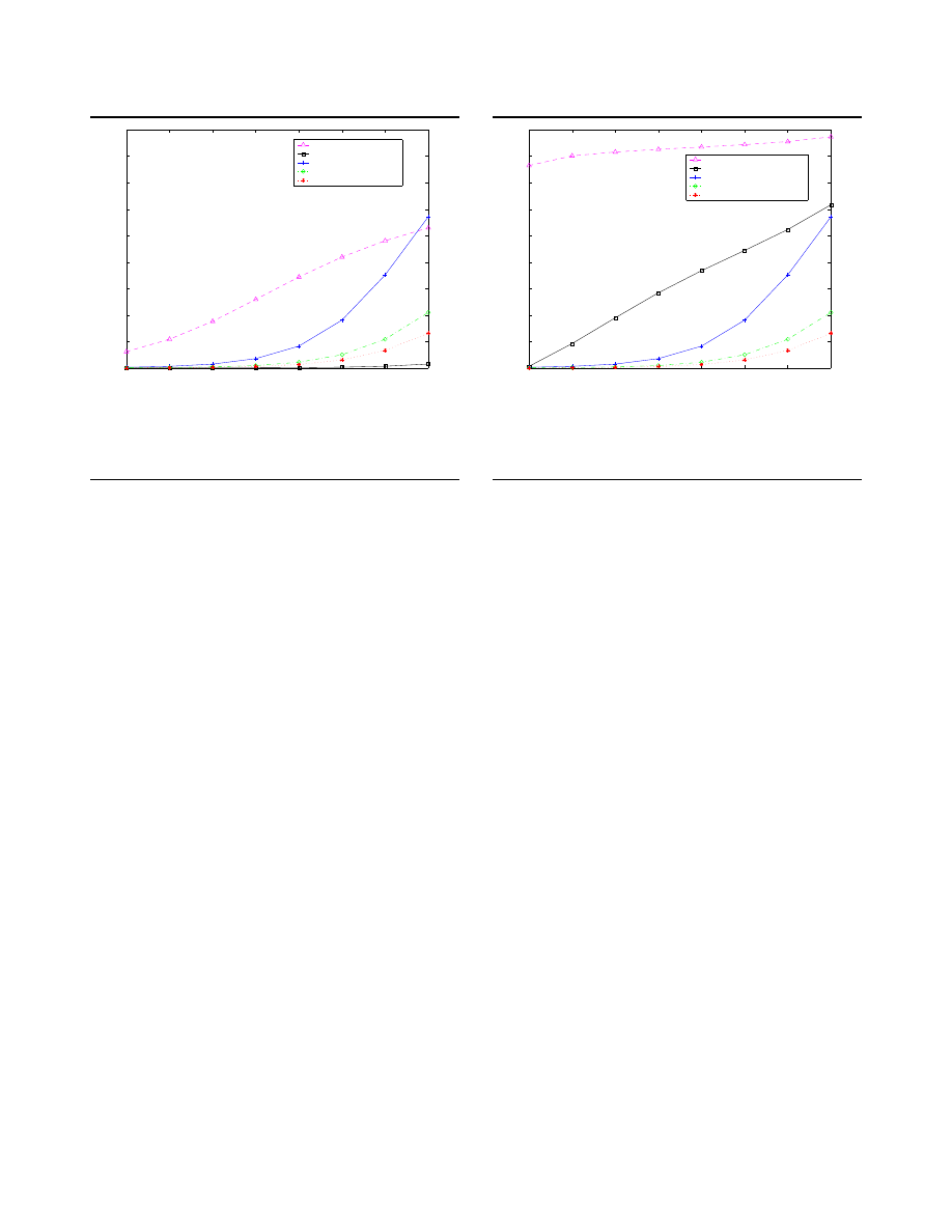
4.2. Content Filtering

Figure 6 shows infections for content filtering de-

ployed in the top N

= 10 and top N

= 30 most con-

nected ASes, and compares it to a patching counter
worm and nullifying with response population I

1000. With N

= 10 deployment the system blocks

90.8% of the AS-to-AS paths, 91.2% of the IP-to-IP
paths, and 9% of the susceptible population in the net-
work; with N

= 30 it blocks 98.7% of the AS-to-AS

paths, 96.7% of the IP-to-IP paths, and 16% of the sus-
ceptibles.

The results indicate that if content filtering deploy-

ment is limited to a small number (ten here) of core
ASes, even though more than 90% of the paths are
blocked, enough infections can slip through to make it
less effective in limiting infections than a swift counter-
worm response. However, increasing deployment to the
top 30 ASes, leading to a seemingly modest 5% in-
crease in blocked paths, dramatically improves effec-
tiveness (a reduction from over 50% to a few percent
for a 4 hour response time) making it better than the
counter-worms.

4.3. Address Blacklisting

Figure 7 compares core deployed address blacklisting

with counter-worms. Address blacklisting is arguably
the more likely containment method to be implemented
soon, being implementable with current technology,
but these results indicate that for a small number
of participating core ASes counter-worms could be
more effective in limiting infections. As deployment

0.5

1.5

2.5

3.5

Response time [h]

% infected hosts

address blacklisting, top 10 ASes
address blacklisting, top 30 ASes
patching worm, I

=1000

nullifying worm, I

=1000

sniper worm, I

=1000

Figure 7. Infections after 24 hours for core de-
ployed address blacklisting compared to counter-
worms (with I

= 1000).

increases, however, the effectiveness improves signifi-
cantly and is primarily limited by the response delay
time.

5. Conclusions

We have modeled content filtering and address

blacklisting (“passive”) defenses and patching and nul-
lifying counter-worms (“active” defenses) to com-
pare their effectiveness in terms of their ability to
prevent worm infections. In all cases a quick re-
sponse is crucial to prevent hosts from becoming in-
fected. For a counter-worm strategy to be effective
it also needs a relatively aggressive launch popula-
tion, and for our comparisons we have assumed a
response population of 1000 worms. Given a quick re-
sponse, numerical results from our models indicate
that:

•

A content filtering defense deployed in customer
networks to protect at least 89% of the hosts, lim-
its infections more than either counter-worm with
the given response population.

•

An address filtering defense deployed in customer
networks needs virtually perfect deployment to be
more effective than a patching counter-worms, and
cannot outperform a nullifying worm.

•

A content filtering defense deployed in the 30 most
connected ASes can outperform the active defense,
while that level of deployment is less effective for
address based blocking.

We also derived one result for the case of customer de-
ployed content filtering versus a patching worm that
relates the initial conditions of the original worm at-
tack to the protection effectiveness for a given set of
response parameters.

In this study we have not explicitly factored in other

issues related to active measures, such as impact on
the network. These factors were discussed in a related
study [15]; and ultimately, one would need to take such
issues, as well as legal and ethical aspects, into account.
However, given the current lack of a defensive infras-
tructure, we speculate that active measures might be a
feasible option, as a last resort, for large networks under
single ownership, if it could be done in a reliable man-
ner. Whether this is practical remains an open ques-
tion.

Acknowledgments We thank Ken Eichman at the
Chemical Abstract Service for Code Red data and
the Route Views project at the University of Ore-
gon for BGP routing data.

References

[1] RIPE Network Coordination Centre. Routing Infor-

mation Service. http://ris.ripe.net, last accessed,
March 2004.

[2] Z. Chen, L. Gao, and K. Kwiat. Modeling the spread of

active worms. INFOCOM 2003, 2003.

[3] Cisco.

Dealing with mallocfail and high cpu uti-

lization

resulting

from

the

“code

red”

worm.

http://www.cisco.com/warp/public/-63/
ts codred worm.shtml

, October 2001.

[4] D.J. Daley and J. Gani. Epidemic Modelling: An Intro-

duction. Cambridge University Press, Cambridge, UK,
1999.

[5] P. Ferrie, P. Sz¨

or, and F. Perriot.

Worm wars.

Virus

Bulletin

(www.virusbtn.com),

Oct.

2003.

http://www.virusbtn.com/resources/viruses/
indepth/welchia.xml

[Last accessed March 30, 2004.].

[6] L. Gao. On Inferring Automonous System Relationships

in the Internet. IEEE Global Internet, Nov. 2000.

[7] L. Gao and J. Rexford. Stable Internet Routing With-

out Global Coordination. IEEE/ACM Transactions on
Networking, Vol. 9, No. 6, Dec. 2001.

[8] M. Garetto, W. Gong, and D. Towsley. Modeling Mal-

ware Spreading Dynamics. INFOCOM 2003. Twenty-
Second Annual Joint Conference of the IEEE Computer
and Communications Societies. Pages:1869 - 1879 vol.3,
April 2003.

[9] M. Liljenstam, D. Nicol, V. Berk, and B. Gray. Simulat-

ing realistic network worm traffic for worm warning sys-
tem design and testing. in Proc. of the First ACM Work-
shop on Rapid Malcode (WORM’03), Oct 2003.

[10] D. Meyer. University of Oregon Route Views Project.

http://antc.uoregon.edu/route-views/, May 2002.

[11] D. Moore, V. Paxson, S. Savage, C. Shannon, S. Stan-

iford, and N. Weaver.

The spread of the sap-

phire/slammer

worm.

http://www.caida.org/

outreach/papers/2003/sapphire/ sapphire.html

2003.

[12] D. Moore, C. Shannon, and K. Claffy. Code-red: a case

study on the spread and victims of an internet worm. in
Proc. of the Internet Measurement Workshop (IMW),
Marseille, France, Nov 2002. ACM Press.

[13] D. Moore, C. Shannon, G. Voelker, and S. Savage. In-

ternet quarantine: Requirements for containing self-
propagating code. In Proceedings of the 22nd Annual
Joint Conference of the IEEE Computer and Communi-
cations Societies (INFOCOM 2003), April 2003.

[14] M. E. J. Newman, S. Forrest, and J. Balthrop. Email

Networks and the Spread of Computer Viruses. Physical
Review E, 66:035101(R), Sept. 2002.

[15] D. Nicol and M. Liljenstam. Models of Active Worm De-

fenses. Technical Report UILU-ENG-04-2204 (CRHC-
04-04), June 2004.

[16] R. Pastor-Satorras and A. Vespignani.

Epidemic

Spreading in Scale-free Networks. Physical Review Let-
ters, 86(14):3200–3203, April 2001.

[17] Eeye Digital Security. Blaster worm analysis. Advisory

AL20030811 http://www.eeye.com/html/Research/
Advisories/AL20030811.html

, Aug. 2003.

[18] S. Staniford, V. Paxson, and N. Weaver.

How

to Own the Internet in Your Spare Time.

Proc. of the USENIX Security Symposium, 2002.
http://www.icir.org/vern/papers/cdc-usenix-
sec02/index.html.

[19] H. Toyoizumi and A. Kara. Predators: good will mobile

codes combat against computer viruses. Proceedings of
the 2002 workshop on New security paradigms, 2002.

[20] A. Wagner, T. D ubendorfer, B. Plattner, and R. Hies-

tand. Experiences with worm propagation simulations.
in Proc. of the First ACM Workshop on Rapid Malcode
(WORM’03), Oct 2003.

[21] F. Wang and L. Gao. Inferring and Characterizing Inter-

ent Routing Policies. ACM SIGCOMM Internet Mea-
surement Workshop, 2003.

[22] Y. Wang, D. Chakrabarti, C. Wang, and C. Faloutsos.

Epidemic Spreading in Real Networks: An Eigenvalue
Viewpoint. 22nd Symposium on Reliable Distributed
Computing (SRDS2003), Florence, Italy, Oct. 2003.

[23] J. Wu, S. Vangala, L. Gao, and K. Kwiat. An effective ar-

chitecture and algorithm for detecting worms with var-
ious scan techniques. Network and Distributed System
Security Symposium, 2004.

[24] C. Zou, L. Gao, W. Gong, and D. Towsley. Monitor-

ing and early warning for internet worms. In Proceed-
ings of 10th ACM Conference on Computer and Com-
munication Security (CCS’03), 2003.

[25] C. Zou, W. Gong, and D. Towsley. Worm propagation

modeling and analysis under dynamic quarantine de-
fense. in Proc. of the First ACM Workshop on Rapid
Malcode (WORM’03), Oct 2003.

Wyszukiwarka

Podobne podstrony:
Models of Active Worm Defenses
Taxonomy and Effectiveness of Worm Defense Strategies
Comparative testing and evaluation of hard surface disinfectants
A comparison?tween English and German and their ancestors
Passive versus active stretching
Shield A First Line Worm Defense
Mark Harrison Guns and Rubles, The Defense Industry in the Stalinist State (2008)
Simulating and optimising worm propagation algorithms
The Cornell Commission On Morris and the Worm
Feedback Email Worm Defense System for Enterprise Networks
Genolevures comparative genomics and molecular evolution of yeast
On Deriving Unknown Vulnerabilities from Zero Day Polymorphic and Metamorphic Worm Exploits
Comparative testing and evaluation of hard surface disinfectants
Comparing Weight and Hight
active and passive voice
Active and Passive Voice Exercise I
Implications of Peer to Peer Networks on Worm Attacks and Defenses
Active and passive(past) busuu
Active and passive(future) busuu

więcej podobnych podstron