
In: Infectious Disease Modelling Research Progress
Editors: J.M. Tchuenche and C. Chiyaka, pp. 133-150
ISBN 978-1-60741-347-9
c
2009 Nova Science Publishers, Inc.
Chapter 4
W
HEN
Z
OMBIES
A
TTACK
!: M
ATHEMATICAL
M
ODELLING OF AN
O
UTBREAK OF
Z
OMBIE
I
NFECTION
Philip Munz
1∗
, Ioan Hudea
1†
, Joe Imad
2‡
, Robert J. Smith?
3§
1
School of Mathematics and Statistics, Carleton University,
1125 Colonel By Drive, Ottawa, ON K1S 5B6, Canada
2
Department of Mathematics, The University of Ottawa,
585 King Edward Ave, Ottawa ON K1N 6N5, Canada
2
Department of Mathematics and Faculty of Medicine, The University of Ottawa,
585 King Edward Ave, Ottawa ON K1N 6N5, Canada
Abstract
Zombies are a popular figure in pop culture/entertainment and they are usually
portrayed as being brought about through an outbreak or epidemic. Consequently,
we model a zombie attack, using biological assumptions based on popular zombie
movies. We introduce a basic model for zombie infection, determine equilibria and
their stability, and illustrate the outcome with numerical solutions. We then refine the
model to introduce a latent period of zombification, whereby humans are infected, but
not infectious, before becoming undead. We then modify the model to include the
effects of possible quarantine or a cure. Finally, we examine the impact of regular,
impulsive reductions in the number of zombies and derive conditions under which
eradication can occur. We show that only quick, aggressive attacks can stave off the
doomsday scenario: the collapse of society as zombies overtake us all.
1.
Introduction
A zombie is a reanimated human corpse that feeds on living human flesh [1]. Stories
about zombies originated in the Afro-Caribbean spiritual belief system of Vodou (anglicised
∗
E-mail address: pmunz@connect.carleton.ca
†
E-mail address: iahudea@connect.carleton.ca
‡
E-mail address: jimad050@uottawa.ca
§
E-mail address: rsmith43@uottawa.ca. Corresponding author.

134
Philip Munz, Ioan Hudea, Joe Imad et al.
voodoo). These stories described people as being controlled by a powerful sorcerer. The
walking dead became popular in the modern horror fiction mainly because of the success
of George A. Romero’s 1968 film, Night of the Living Dead [2]. There are several possible
etymologies of the word zombie. One of the possible origins is jumbie, which comes from
the Carribean term for ghost. Another possible origin is the word nzambi which in Kongo
means ‘spirit of a dead person’. According to the Merriam-Webster dictionary, the word
zombie originates from the word zonbi, used in the Louisiana Creole or the Haitian Creole.
According to the Creole culture, a zonbi represents a person who died and was then brought
to life without speech or free will.
The followers of Vodou believe that a dead person can be revived by a sorcerer [3].
After being revived, the zombies remain under the control of the sorcerer because they
have no will of their own. Zombi is also another name for a Voodoo snake god. It is said
that the sorcerer uses a ‘zombie powder’ for the zombification. This powder contains an
extremely powerful neurotoxin that temporarily paralyzes the human nervous system and
it creates a state of hibernation. The main organs, such as the heart and lungs, and all of
the bodily functions, operate at minimal levels during this state of hibernation. What turns
these human beings into zombies is the lack of oxygen to the brain. As a result of this, they
suffer from brain damage.
A popular belief in the Middle Ages was that the souls of the dead could return to earth
one day and haunt the living [4]. In France, during the Middle Ages, they believed that the
dead would usually awaken to avenge some sort of crime committed against them during
their life. These awakened dead took the form of an emaciated corpse and they wandered
around graveyards at night. The idea of the zombie also appears in several other cultures,
such as China, Japan, the Pacific, India, Persia, the Arabs and the Americas.
Modern zombies (the ones illustrated in books, films and games [1, 5]) are very dif-
ferent from the voodoo and the folklore zombies. Modern zombies follow a standard, as
set in the movie Night of the Living Dead [2]. The ghouls are portrayed as being mindless
monsters who do not feel pain and who have an immense appetite for human flesh. Their
aim is to kill, eat or infect people. The ‘undead’ move in small, irregular steps, and show
signs of physical decomposition such as rotting flesh, discoloured eyes and open wounds.
Modern zombies are often related to an apocalypse, where civilization could collapse due
to a plague of the undead. The background stories behind zombie movies, video games etc,
are purposefully vague and inconsistent in explaining how the zombies came about in the
first place. Some ideas include radiation (Night of the Living Dead [2]), exposure to air-
borne viruses (Resident Evil [6]), mutated diseases carried by various vectors (Dead Rising
[7] claimed it was from bee stings of genetically altered bees). Shaun of the Dead [8] made
fun of this by not allowing the viewer to determine what actually happened.
When a susceptible individual is bitten by a zombie, it leaves an open wound. The
wound created by the zombie has the zombie’s saliva in and around it. This bodily fluid
mixes with the blood, thus infecting the (previously susceptible) individual.
The zombie that we chose to model was characterised best by the popular-culture zom-
bie. The basic assumptions help to form some guidelines as to the specific type of zombie
we seek to model (which will be presented in the next section). The model zombie is of
the classical pop-culture zombie: slow moving, cannibalistic and undead. There are other
‘types’ of zombies, characterised by some movies like 28 Days Later [9] and the 2004 re-

When Zombies Attack!
135
make of Dawn of the Dead [10]. These ‘zombies’ can move faster, are more independent
and much smarter than their classical counterparts. While we are trying to be as broad as
possible in modelling zombies – especially since there are many varieties – we have decided
not to consider these individuals.
2.
The Basic Model
For the basic model, we consider three basic classes:
• Susceptible (S).
• Zombie (Z).
• Removed (R).
Susceptibles can become deceased through ‘natural’ causes, i.e., non-zombie-related
death (parameter δ). The removed class consists of individuals who have died, either
through attack or natural causes. Humans in the removed class can resurrect and become
a zombie (parameter ζ). Susceptibles can become zombies through transmission via an
encounter with a zombie (transmission parameter β). Only humans can become infected
through contact with zombies, and zombies only have a craving for human flesh so we do
not consider any other life forms in the model. New zombies can only come from two
sources:
• The resurrected from the newly deceased (removed group).
• Susceptibles who have ‘lost’ an encounter with a zombie.
In addition, we assume the birth rate is a constant, Π. Zombies move to the removed class
upon being ‘defeated’. This can be done by removing the head or destroying the brain of
the zombie (parameter α). We also assume that zombies do not attack/defeat other zombies.
Thus, the basic model is given by
S
0
=
Π − βSZ − δS
Z
0
=
βSZ + ζR − αSZ
R
0
=
δS + αSZ − ζR .
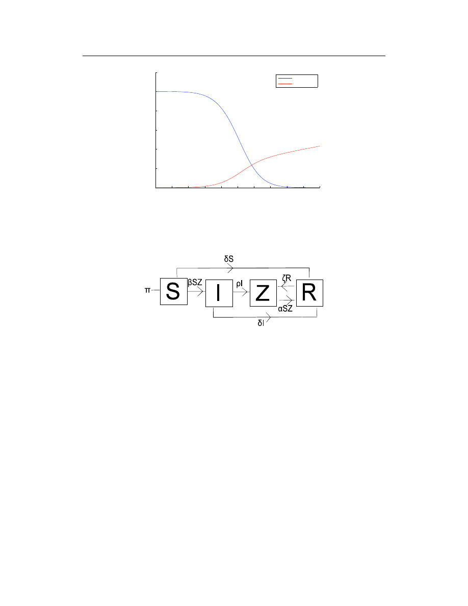
This model is illustrated in Figure 1.
This model is slightly more complicated than the basic SIR models that usually char-
acterise infectious diseases [11], because this model has two mass-action transmissions,
which leads to having more than one nonlinear term in the model. Mass-action incidence
specifies that an average member of the population makes contact sufficient to transmit in-
fection with βN others per unit time, where N is the total population without infection.
In this case, the infection is zombification. The probability that a random contact by a
zombie is made with a susceptible is S/N ; thus, the number of new zombies through this
transmission process in unit time per zombie is:
(βN )(S/N )Z = βSZ .

136
Philip Munz, Ioan Hudea, Joe Imad et al.
Figure 1. The basic model.
We assume that a susceptible can avoid zombification through an altercation with a zombie
by defeating the zombie during their contact, and each susceptible is capable of resisting
infection (becoming a zombie) at a rate α. So, using the same idea as above with the
probability Z/N of random contact of a susceptible with a zombie (not the probability of a
zombie attacking a susceptible), the number of zombies destroyed through this process per
unit time per susceptible is:
(αN )(Z/N )S
=
αSZ .
The ODEs satisfy
S
0
+ Z
0
+ R
0
=
Π
and hence
S + Z + R
→ ∞
as t → ∞, if Π 6= 0. Clearly S 6→ ∞, so this results in a ‘doomsday’ scenario: an outbreak
of zombies will lead to the collapse of civilisation, as large numbers of people are either
zombified or dead.
If we assume that the outbreak happens over a short timescale, then we can ignore birth
and background death rates. Thus, we set Π = δ = 0.
Setting the differential equations equal to 0 gives
−βSZ
=
0
βSZ + ζR − αSZ
=
0
αSZ − ζR
=
0 .
From the first equation, we have either S = 0 or Z = 0. Thus, it follows from S = 0 that
we get the ‘doomsday’ equilibrium
( ¯
S, ¯
Z, ¯
R)
=
(0, ¯
Z, 0) .
When Z = 0, we have the disease-free equilibrium
( ¯
S, ¯
Z, ¯
R)
=
(N, 0, 0) .

When Zombies Attack!
137
These equilibrium points show that, regardless of their stability, human-zombie coexistence
is impossible.
The Jacobian is then
J
=
−βZ
−βS
0
βZ − αZ
βS − αS
ζ
αZ
αS
−ζ
.
The Jacobian at the disease-free equilibrium is
J (N, 0, 0)
=
0
−βN
0
0
βN − αN
ζ
0
αN
−ζ
.
We have
det(J − λI)
=
−λ{λ
2
+ [ζ − (β − α)N ]λ − βζN } .
It follows that the characteristic equation always has a root with positive real part. Hence,
the disease-free equilibrium is always unstable.
Next, we have
J (0, ¯
Z, 0)
=
−β ¯
Z
0
0
β ¯
Z − α ¯
Z
0
ζ
α ¯
Z
0
−ζ
.
Thus,
det(J − λI)
=
−λ(−β ¯
Z − λ)(−ζ − λ) .
Since all eigenvalues of the doomsday equilibrium are negative, it is asymptotically stable.
It follows that, in a short outbreak, zombies will likely infect everyone.
In the following figures, the curves show the interaction between susceptibles and zom-
bies over a period of time. We used Euler’s method to solve the ODE’s. While Euler’s
method is not the most stable numerical solution for ODE’s, it is the easiest and least time-
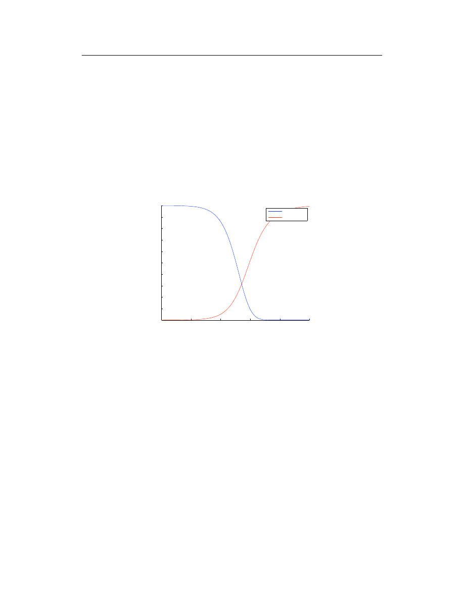
consuming. See Figures 2 and 3 for these results. The MATLAB code is given at the end
of this chapter. Values used in Figure 3 were α = 0.005, β = 0.0095, ζ = 0.0001 and
δ = 0.0001.
3.
The Model with Latent Infection
We now revise the model to include a latent class of infected individuals. As discussed in
Brooks [1], there is a period of time (approximately 24 hours) after the human susceptible
gets bitten before they succumb to their wound and become a zombie.
We thus extend the basic model to include the (more ‘realistic’) possibility that a sus-
ceptible individual becomes infected before succumbing to zombification. This is what is
seen quite often in pop-culture representations of zombies ([2, 6, 8]).
Changes to the basic model include:

138
Philip Munz, Ioan Hudea, Joe Imad et al.
0
1
2
3
4
5
6
7
8
9
10
0
100
200
300
400
500
600
Time
Population Value (1000’s)
Basic model ! R0 < 1 with I.C. = DFE
Suscepties
Zombies
Figure 2. The case of no zombies. However, this equilibrium is unstable.
• Susceptibles first move to an infected class once infected and remain there for some
period of time.
• Infected individuals can still die a ‘natural’ death before becoming a zombie; other-
wise, they become a zombie.
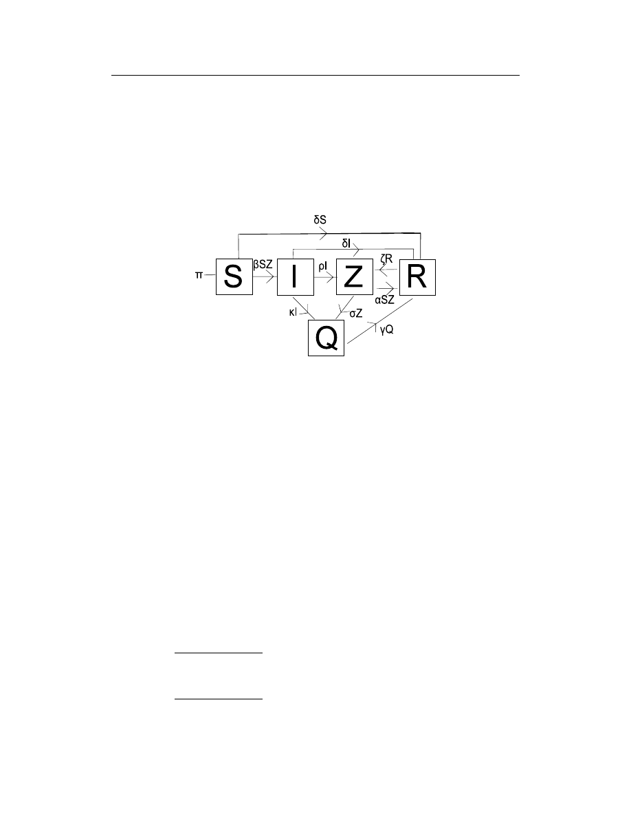
We shall refer to this as the SIZR model. The model is given by
S
0
=
Π − βSZ − δS
I
0
=
βSZ − ρI − δI
Z
0
=
ρI + ζR − αSZ
R
0
=
δS + δI + αSZ − ζR
The SIZR model is illustrated in Figure 4
As before, if Π 6= 0, then the infection overwhelms the population. Consequently, we
shall again assume a short timescale and hence Π = δ = 0. Thus, when we set the above
equations to 0, we get either S = 0 or Z = 0 from the first equation. It follows again from
our basic model analysis that we get the equilibria:
Z = 0
=⇒
( ¯
S, ¯
I, ¯
Z, ¯
R)
=
(N, 0, 0, 0)
S = 0
=⇒
( ¯
S, ¯
I, ¯
Z, ¯
R)
=
(0, 0, ¯
Z, 0)
Thus, coexistence between humans and zombies/infected is again not possible.
In this case, the Jacobian is
J
=
−βZ
0
−βS
0
βZ
−ρ
βS
0
−αZ
ρ
−αS
ζ
αZ
0
αS
−ζ
.
When Zombies Attack!
139
0
0.5
1
1.5
2
2.5
3
3.5
4
4.5
5
0
100
200
300
400
500
600
Time
Population Values (1000’s)
Basic Model! R0 > 1 with IC = DFE
Suscepties
Zombies
Figure 3. Basic model outbreak scenario. Susceptibles are quickly eradicated and zombies
take over, infecting everyone.
Figure 4. The SIZR model flowchart: the basic model with latent infection.
First, we have
det(J (N, 0, 0, 0) − λI)
=
det
−λ
0
−βN
0
0
−ρ − λ
βN
0
0
ρ
−αN − λ
ζ
0
0
αN
−ζ − λ
=
−λ det
−ρ − λ
βN
0
ρ
−αN − λ
ζ
0
αN
−ζ − λ
=
−λ
−λ
3
− (ρ + ζ + αN )λ
2
− (ραN + ρζ − ρβN )λ
+ρζβN ] .
Since ρζβN > 0, it follows that det(J (N, 0, 0, 0) − λI) has an eigenvalue with positive
real part. Hence, the disease-free equilibrium is unstable.
140
Philip Munz, Ioan Hudea, Joe Imad et al.
Next, we have
det(J (0, 0, ¯
Z, 0) − λI)
=
det
−β ¯
Z − λ
0
0
0
β ¯
Z
−ρ − λ
0
0
−α ¯
Z
ρ
−λ
ζ
α ¯
Z
0
0
−ζ − λ
.
The eigenvalues are thus λ = 0, −β ¯
Z, −ρ, −ζ. Since all eigenvalues are nonpositive, it
follows that the doomsday equilibrium is stable. Thus, even with a latent period of infection,
zombies will again take over the population.
We plotted numerical results from the data again using Euler’s method for solving the
ODEs in the model. The parameters are the same as in the basic model, with ρ = 0.005.
See Figure 5. In this case, zombies still take over, but it takes approximately twice as long.
0
2
4
6
8
10
0
50
100
150
200
250
300
350
400
450
500
Time
Population Values (1000’s)
SIZR Model! R0 > 1 with IC = DFE
(same values for parameters used in previous figure)
Suscepties
Zombies
Figure 5. An outbreak with latent infection.
4.
The Model with Quarantine
In order to contain the outbreak, we decided to model the effects of partial quarantine of
zombies. In this model, we assume that quarantined individuals are removed from the
population and cannot infect new individuals while they remain quarantined. Thus, the
changes to the previous model include:
• The quarantined area only contains members of the infected or zombie populations
(entering at rates κ and σ, respectively).
• There is a chance some members will try to escape, but any that tried to would be
killed before finding their ‘freedom’ (parameter γ).
• These killed individuals enter the removed class and may later become reanimated as
‘free’ zombies.
When Zombies Attack!
141
The model equations are:
S
0
=
Π − βSZ − δS
I
0
=
βSZ − ρI − δI − κI
Z
0
=
ρI + ζR − αSZ − σZ
R
0
=
δS + δI + αSZ − ζR + γQ
Q
0
=
κI + σZ − γQ .
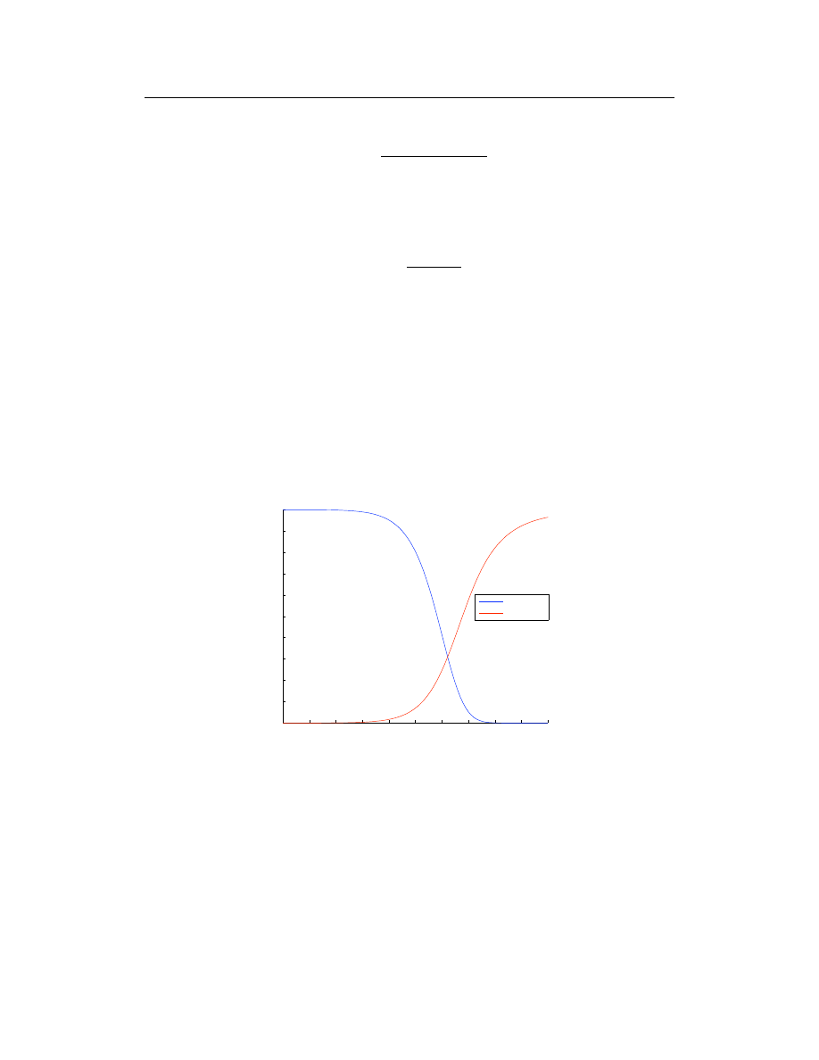
The model is illustrated in Figure 6.
Figure 6. Model flow diagram for the Quarantine model.
For a short outbreak (Π = δ = 0), we have two equilibria,
( ¯
S, ¯
I, ¯
Z, ¯
R, ¯
Q) = (N, 0, 0, 0, 0), (0, 0, ¯
Z, ¯
R, ¯
Q) .
In this case, in order to analyse stability, we determined the basic reproductive ratio, R
0
[12] using the next-generation method [13]. The basic reproductive ratio has the property
that if R
0
> 1, then the outbreak will persist, whereas if R
0
< 1, then the outbreak will be
eradicated.
If we were to determine the Jacobian and evaluate it at the disease-free equilibrium, we
would have to evaluate a nontrivial 5 by 5 system and a characteristic polynomial of degree
of at least 3. With the next-generation method, we only need to consider the infective
differential equations I
0
, Z
0
and Q
0
. Here, F is the matrix of new infections and V is the
matrix of transfers between compartments, evaluated at the disease-free equilibrium.
F =
0
βN
0
0
0
0
0
0
0
,
V =
ρ + κ
0
0
−ρ
αN + σ
0
−κ
−σ
γ
V
−1
=
1
γ(ρ + κ)(αN + σ)
γ(αN + σ)
0
0
ργ
γ(ρ + κ)
0
ρσ + κ(αN + σ)
σ(ρ + κ)
(ρ + κ)(αN + σ)
F V
−1
=
1
γ(ρ + κ)(αN + σ)
βN ργ
βN γ(ρ + κ)
0
0
0
0
0
0
0
.
142
Philip Munz, Ioan Hudea, Joe Imad et al.
This gives us
R
0
=
βN ρ
(ρ + κ)(αN + σ)
.
It follows that the disease-free equilibrium is only stable if R
0
< 1. This can be
achieved by increasing κ or σ, the rates of quarantining infected and zombified individ-
uals, respectively. If the population is large, then
R
0
≈
βρ
(ρ + κ)α
.
If β > α (zombies infect humans faster than humans can kill them, which we expect), then
eradication depends critically on quarantining those in the primary stages of infection. This
may be particularly difficult to do, if identifying such individuals is not obvious [8].
However, we expect that quarantining a large percentage of infected individuals is un-
realistic, due to infrastructure limitations. Thus, we do not expect large values of κ or σ, in
practice. Consequently, we expect R
0
> 1.
As before, we illustrate using Euler’s method. The parameters were the same as those
used in the previous models. We varied κ, σ, γ to satisfy R
0
> 1. The results are illustrated
in Figure 7. In this case, the effect of quarantine is to slightly delay the time to eradication
of humans.
0
1
2
3
4
5
6
7
8
9
10
0
50
100
150
200
250
300
350
400
450
500
Time
Population Values (1000’s)
SIZRQ Model! R0 > 1 with IC = DFE
(same values for parameters used in previous figure)
Suscepties
Zombies
Figure 7. An outbreak with quarantine.
The fact that those individuals in Q were destroyed made little difference overall to the
analysis as our intervention (i.e., destroying the zombies) did not have a major impact to
the system (we were not using Q to eradicate zombies). It should also be noted that we still
expect only two outcomes: either zombies are eradicated, or they take over completely.
Notice that, in Figure 7 at t = 10, there are fewer zombies than in the Figure 5 at t = 10.
This is explained by the fact that the numerics assume that the Quarantine class continues
When Zombies Attack!
143
to exist, and there must still be zombies in that class. The zombies measured by the curve
in the figure are considered the ‘free’ zombies: the ones in the Z class and not in Q.
5.
A Model with Treatment
Suppose we are able to quickly produce a cure for ‘zombie-ism’. Our treatment would
be able to allow the zombie individual to return to their human form again. Once human,
however, the new human would again be susceptible to becoming a zombie; thus, our cure
does not provide immunity. Those zombies who resurrected from the dead and who were
given the cure were also able to return to life and live again as they did before entering the
R class.
Things that need to be considered now include:
• Since we have treatment, we no longer need the quarantine.
• The cure will allow zombies to return to their original human form regardless of how
they became zombies in the first place.
• Any cured zombies become susceptible again; the cure does not provide immunity.
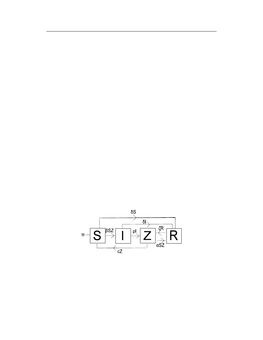
Thus, the model with treatment is given by
S
0
=
Π − βSZ − δS + cZ
I
0
=
βSZ − ρI − δI
Z
0
=
ρI + ζR − αSZ − cZ
R
0
=
δS + δI + αSZ − ζR .
The model is illustrated in Figure 8.
Figure 8. Model flowchart for the SIZR model with cure.
As in all other models, if Π 6= 0, then S + I + Z + R → ∞, so we set Π = δ = 0.
When Z = 0, we get our usual disease-free equilibrium,
( ¯
S, ¯
I, ¯
Z, ¯
R) = (N, 0, 0, 0) .

144
Philip Munz, Ioan Hudea, Joe Imad et al.
However, because of the cZ term in the first equation, we now have the possibility of an
endemic equilibrium ( ¯
S, ¯
I, ¯
Z, ¯
R) satisfying
−β ¯
S ¯
Z + c ¯
Z
=
0
β ¯
S ¯
Z − ρ ¯
I
=
0
ρ ¯
I + ζ ¯
R − α ¯
S ¯
Z − c ¯
Z
=
0
α ¯
S ¯
Z − ζ ¯
R
=
0 .
Thus, the equilibrium is
( ¯
S, ¯
I, ¯
Z, ¯
R)
=
c
β
,
c
ρ
¯
Z, ¯
Z,
αc
ζβ
¯
Z
.
The Jacobian is
J
=
βZ
0
−βS + c
0
βZ
−ρ
βS
0
−αZ
ρ
−αS − c
ζ
αZ
0
αS
−ζ
.
We thus have
det(J ( ¯
S, ¯
I, ¯
Z, ¯
R) − λI)
=
det
β ¯
Z
0
0
0
β ¯
Z
−ρ
c
0
−α ¯
Z
ρ
−
αc
β
− c
ζ
α ¯
Z
0
αc
β
−ζ
=
−(β ¯
Z − λ) det
−ρ
c
0
ρ
−
αc
β
− c
ζ
0
αc
β
−ζ
=
−(β ¯
Z − λ)
−λ
λ
2
+
ρ +
αc
β
+ c + ζ
λ
+
ζαc
β
+
ραc
β
+ ρζ + cζ
.
Since the quadratic expression has only positive coefficients, it follows that there are no
positive eigenvalues. Hence, the coexistence equilibrium is stable.
The results are illustrated in Figure 9. In this case, humans are not eradicated, but only
exist in low numbers.
6.
Impulsive Eradication
Finally, we attempted to control the zombie population by strategically destroying them at
such times that our resources permit (as suggested in [14]). It was assumed that it would
be difficult to have the resources and coordination, so we would need to attack more than
once, and with each attack, try and destroy more zombies. This results in an impulsive
effect [15, 16, 17, 18].
When Zombies Attack!
145
0
2
4
6
8
10
0
50
100
150
200
250
300
350
400
450
500
Time
Population Values (1000’s)
SIZR with Cure ! R0 > 1 with IC = DFE
(same values for parameters used in previous figure)
Suscepties
Zombies
Figure 9. The model with treatment, using the same parameter values as the basic model.
Here, we returned to the basic model and added the impulsive criteria:
S
0
=
Π − βSZ − δS
t
6=
t
n
Z
0
=
βSZ + ζR − αSZ
t
6=
t
n
R
0
=
δS + αSZ − ζR
t
6=
t
n
∆Z
=
−knZ
t
=
t
n
,
where k ∈ (0, 1] is the kill ratio and n denotes the number of attacks required until kn > 1.
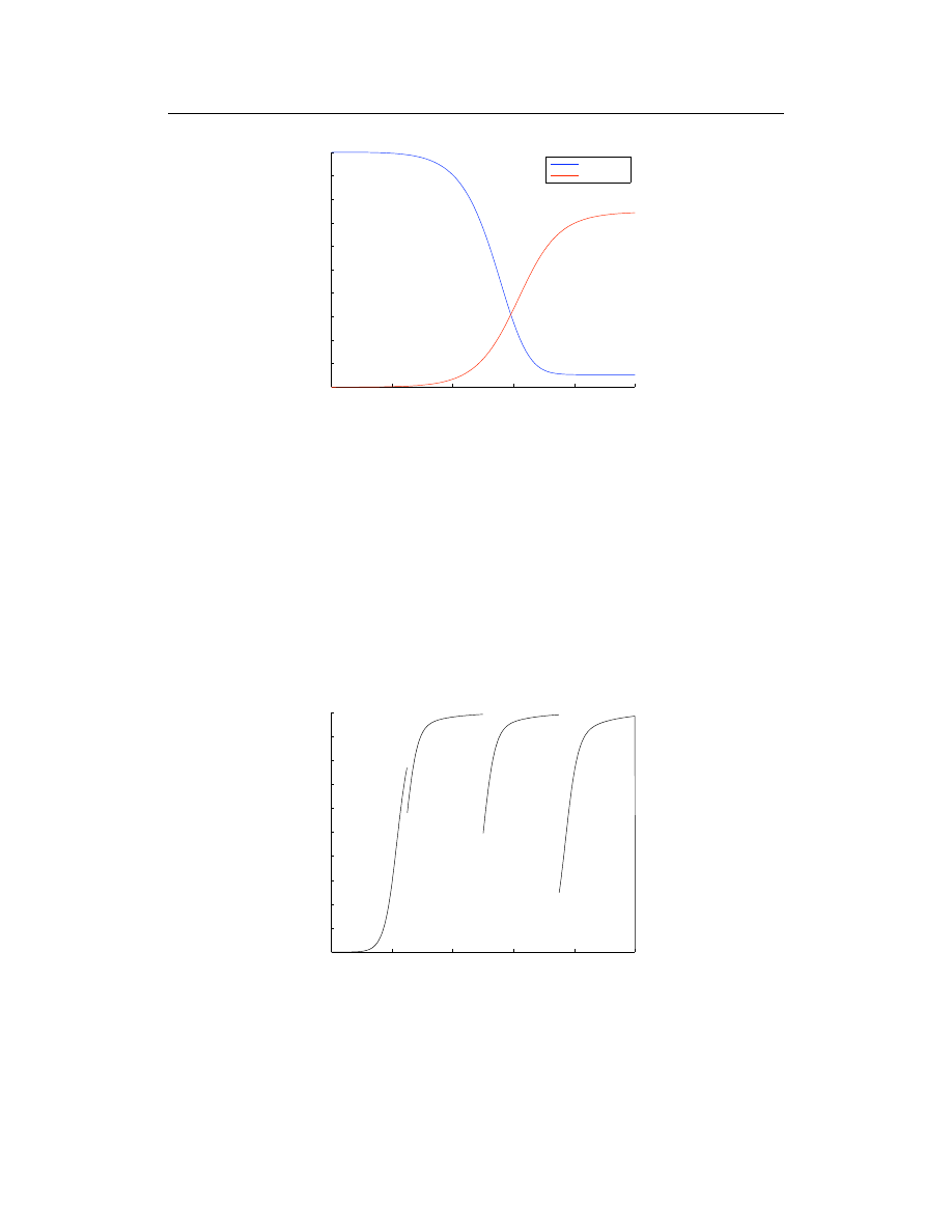
The results are illustrated in Figure 10.
0
2
4
6
8
10
0
100
200
300
400
500
600
700
800
900
1000
Number of Zombies
Time
Eradication with increasing kill ratios
Figure 10. Zombie eradication using impulsive attacks.
In Figure 10, we used k = 0.25 and the values of the remaining parameters were

146
Philip Munz, Ioan Hudea, Joe Imad et al.
(α, β, ζ, δ) = (0.0075, 0.0055, 0.09, 0.0001). Thus, after 2.5 days, 25% of zombies are
destroyed; after 5 days, 50% of zombies are destroyed; after 7.5 days, 75% of remaining
zombies are destroyed; after 10 days, 100% of zombies are destroyed.
7.
Discussion
An outbreak of zombies infecting humans is likely to be disastrous, unless extremely ag-
gressive tactics are employed against the undead. While aggressive quarantine may eradi-
cate the infection, this is unlikely to happen in practice. A cure would only result in some
humans surviving the outbreak, although they will still coexist with zombies. Only suf-
ficiently frequent attacks, with increasing force, will result in eradication, assuming the
available resources can be mustered in time.
Furthermore, these results assumed that the timescale of the outbreak was short, so that
the natural birth and death rates could be ignored. If the timescale of the outbreak increases,
then the result is the doomsday scenario: an outbreak of zombies will result in the collapse
of civilisation, with every human infected, or dead. This is because human births and
deaths will provide the undead with a limitless supply of new bodies to infect, resurrect
and convert. Thus, if zombies arrive, we must act quickly and decisively to eradicate them
before they eradicate us.
The key difference between the models presented here and other models of infectious
disease is that the dead can come back to life. Clearly, this is an unlikely scenario if taken
literally, but possible real-life applications may include allegiance to political parties, or
diseases with a dormant infection.
This is, perhaps unsurprisingly, the first mathematical analysis of an outbreak of zom-
bie infection. While the scenarios considered are obviously not realistic, it is nevertheless
instructive to develop mathematical models for an unusual outbreak. This demonstrates
the flexibility of mathematical modelling and shows how modelling can respond to a wide
variety of challenges in ‘biology’.
In summary, a zombie outbreak is likely to lead to the collapse of civilisation, unless it
is dealt with quickly. While aggressive quarantine may contain the epidemic, or a cure may
lead to coexistence of humans and zombies, the most effective way to contain the rise of
the undead is to hit hard and hit often. As seen in the movies, it is imperative that zombies
are dealt with quickly, or else we are all in a great deal of trouble.
Acknowledgements
We thank Shoshana Magnet, Andy Foster and Shannon Sullivan for useful discussions.
RJS? is supported by an NSERC Discovery grant, an Ontario Early Researcher Award and
funding from MITACS.
function [ ] = zombies(a,b,ze,d,T,dt)
% This function will solve the system of ODE’s for the basic model used in
% the Zombie Dynamics project for MAT 5187.
It will then plot the curve of
% the zombie population based on time.
% Function Inputs: a - alpha value in model: "zombie destruction" rate
%
b - beta value in model: "new zombie" rate

When Zombies Attack!
147
%
ze - zeta value in model: zombie resurrection rate
%
d - delta value in model: background death rate
%
T - Stopping time
%
dt - time step for numerical solutions
% Created by Philip Munz, November 12, 2008
%Initial set up of solution vectors and an initial condition
N = 500;
%N is the population
n = T/dt;
t = zeros(1,n+1);
s = zeros(1,n+1);
z = zeros(1,n+1);
r = zeros(1,n+1);
s(1) = N;
z(1) = 0;
r(1) = 0;
t = 0:dt:T;
% Define the ODE’s of the model and solve numerically by Euler’s method:
for i = 1:n
s(i+1) = s(i) + dt*(-b*s(i)*z(i));
%here we assume birth rate
= background deathrate, so only term is -b term
z(i+1) = z(i) + dt*(b*s(i)*z(i) -a*s(i)*z(i) +ze*r(i));
r(i+1) = r(i) + dt*(a*s(i)*z(i) +d*s(i) - ze*r(i));
if s(i)<0 || s(i) >N
break
end
if z(i) > N || z(i) < 0
break
end
if r(i) <0 || r(i) >N
break
end
end
hold on
plot(t,s,’b’);
plot(t,z,’r’);
legend(’Suscepties’,’Zombies’)
------------
function [z] = eradode(a,b,ze,d,Ti,dt,s1,z1,r1)
% This function will take as inputs, the initial value of the 3 classes.
% It will then apply Eulers method to the problem and churn out a vector of
% solutions over a predetermined period of time (the other input).
% Function Inputs: s1, z1, r1 - initial value of each ODE, either the
%
actual initial value or the value after the
%
impulse.
%
Ti - Amount of time between inpulses and dt is time step
% Created by Philip Munz, November 21, 2008
k = Ti/dt;
%s = zeros(1,n+1);
%z = zeros(1,n+1);
%r = zeros(1,n+1);

148
Philip Munz, Ioan Hudea, Joe Imad et al.
%t = 0:dt:Ti;
s(1) = s1;
z(1) = z1;
r(1) = r1;
for i=1:k
s(i+1) = s(i) + dt*(-b*s(i)*z(i));
%here we assume birth rate
= background deathrate, so only term is -b term
z(i+1) = z(i) + dt*(b*s(i)*z(i) -a*s(i)*z(i) +ze*r(i));
r(i+1) = r(i) + dt*(a*s(i)*z(i) +d*s(i) - ze*r(i));
end
%plot(t,z)
------------
function [] = erad(a,b,ze,d,k,T,dt)
% This is the main function in our numerical impulse analysis, used in
% conjunction with eradode.m, which will simulate the eradication of
% zombies.
The impulses represent a coordinated attack against zombiekind
% at specified times.
% Function Inputs: a - alpha value in model: "zombie destruction" rate
%
b - beta value in model: "new zombie" rate
%
ze - zeta value in model: zombie resurrection rate
%
d - delta value in model: background death rate
%
k - "kill" rate, used in the impulse
%
T - Stopping time
%
dt - time step for numerical solutions
% Created by Philip Munz, November 21, 2008
N = 1000;
Ti = T/4; %We plan to break the solution into 4 parts with 4 impulses
n = Ti/dt;
m = T/dt;
s = zeros(1,n+1);
z = zeros(1,n+1);
r = zeros(1,n+1);
sol = zeros(1,m+1);
%The solution vector for all zombie impulses and such
t = zeros(1,m+1);
s1 = N;
z1 = 0;
r1 = 0;
%i=0;
%i is the intensity factor for the current impulse
%for j=1:n:T/dt
%
i = i+1;
%
t(j:j+n) = Ti*(i-1):dt:i*Ti;
%
sol(j:j+n) = eradode(a,b,ze,d,Ti,dt,s1,z1,r1);
%
sol(j+n) = sol(j+n)-i*k*sol(j+n);
%
s1 = N-sol(j+n);
%
z1 = sol(j+n+1);
%
r1 = 0;
%end
sol1 = eradode(a,b,ze,d,Ti,dt,s1,z1,r1);
sol1(n+1) = sol1(n+1)-1*k*sol1(n+1);
%347.7975;

When Zombies Attack!
149
s1 = N-sol1(n+1);
z1 = sol1(n+1);
r1 = 0;
sol2 = eradode(a,b,ze,d,Ti,dt,s1,z1,r1);
sol2(n+1) = sol2(n+1)-2*k*sol2(n+1);
s1 = N-sol2(n+1);
z1 = sol2(n+1);
r1 = 0;
sol3 = eradode(a,b,ze,d,Ti,dt,s1,z1,r1);
sol3(n+1) = sol3(n+1)-3*k*sol3(n+1);
s1 = N-sol3(n+1);
z1 = sol3(n+1);
r1 = 0;
sol4 = eradode(a,b,ze,d,Ti,dt,s1,z1,r1);
sol4(n+1) = sol4(n+1)-4*k*sol4(n+1);
s1 = N-sol4(n+1);
z1 = sol4(n+1);
r1 = 0;
sol=[sol1(1:n),sol2(1:n),sol3(1:n),sol4];
t = 0:dt:T;
t1 = 0:dt:Ti;
t2 = Ti:dt:2*Ti;
t3 = 2*Ti:dt:3*Ti;
t4 = 3*Ti:dt:4*Ti;
%plot(t,sol)
hold on
plot(t1(1:n),sol1(1:n),’k’)
plot(t2(1:n),sol2(1:n),’k’)
plot(t3(1:n),sol3(1:n),’k’)
plot(t4,sol4,’k’)
hold off
References
[1] Brooks, Max, 2003 The Zombie Survival Guide - Complete Protection from the Living
Dead
, Three Rivers Press, pp. 2-23.
[2] Romero, George A. (writer, director), 1968 Night of the Living Dead.
[3] Davis, Wade, 1988 Passage of Darkness - The Ethnobiology of the Haitian Zombie,
Simon and Schuster pp. 14, 60-62.
[4] Davis, Wade, 1985 The Serpent and the Rainbow, Simon and Schuster pp. 17-20, 24,
32.
[5] Williams, Tony, 2003 Knight of the Living Dead - The Cinema of George A. Romero,
Wallflower Press pp.12-14.
[6] Capcom, Shinji Mikami (creator), 1996-2007 Resident Evil.
[7] Capcom, Keiji Inafune (creator), 2006 Dead Rising.

150
Philip Munz, Ioan Hudea, Joe Imad et al.
[8] Pegg, Simon (writer, creator, actor), 2002 Shaun of the Dead.
[9] Boyle, Danny (director), 2003 28 Days Later.
[10] Snyder, Zack (director), 2004 Dawn of the Dead.
[11] Brauer, F. Compartmental Models in Epidemiology. In: Brauer, F., van den Driessche,
P., Wu, J. (eds). Mathematical Epidemiology. Springer Berlin 2008.
[12] Heffernan, J.M., Smith, R.J., Wahl, L.M. (2005). Perspectives on the Basic Reproduc-
tive Ratio. J R Soc Interface 2(4), 281-293.
[13] van den Driessche, P., Watmough, J. (2002) Reproduction numbers and sub-threshold
endemic equilibria for compartmental models of disease transmission. Math. Biosci.
180, 29-48.
[14] Brooks, Max, 2006 World War Z - An Oral History of the Zombie War, Three Rivers
Press.
[15] Bainov, D.D. & Simeonov, P.S. Systems with Impulsive Effect. Ellis Horwood Ltd,
Chichester (1989).
[16] Bainov, D.D. & Simeonov, P.S. Impulsive differential equations: periodic solutions
and applications
. Longman Scientific and Technical, Burnt Mill (1993).
[17] Bainov, D.D. & Simeonov, P.S. Impulsive Differential Equations: Asymptotic Proper-
ties of the Solutions.
World Scientific, Singapore (1995).
[18] Lakshmikantham, V., Bainov, D.D. & Simeonov, P.S. Theory of Impulsive Differential
Equations
. World Scientific, Singapore (1989).
Wyszukiwarka
Podobne podstrony:
(ebook PDF)Shannon A Mathematical Theory Of Communication RXK2WIS2ZEJTDZ75G7VI3OC6ZO2P57GO3E27QNQ
Dance, Shield Modelling of sound ®elds in enclosed spaces with absorbent room surfaces
01 Mathematical model of power network
R 6 2 1 Mathematical model of enterprise, przyklad 1
(ebook PDF)Shannon A Mathematical Theory Of Communication RXK2WIS2ZEJTDZ75G7VI3OC6ZO2P57GO3E27QNQ
Dance, Shield Modelling of sound ®elds in enclosed spaces with absorbent room surfaces
Modelling of dehydration rehydration of orange slices in combined microwaveair drying
The Costs of Hospital Infection
Describe the role of the dental nurse in minimising the risk of cross infection during and after the
Philosophy Of Mind Minds,Machines,And Mathematics A Review Of Shadows Of The Mind By Roger Penrose
Harrison, Harry & Haldeman, Jack C Bill 5 Bill on the Planet of Zombie Vampires
Cinlar E , Vanderbei R Mathematical Methods of Engineering Analysis
Harry Harrison Bill 05 On the Planet of Zombie Vampires (Jack C Haldeman)
Mathematical Model of Computer Viruses
Thin layer modelling of the convective, microwave, microwave convective and microwave vacuum drying
Epidemiological Modelling of Peer to Peer Viruses and Pollution
więcej podobnych podstron