
arXiv:hep-th/0011110 v2 30 Nov 2000
EFI-2000-45
TASI Lectures: Cosmology for String Theorists
Sean M. Carroll
Enrico Fermi Institute and Department of Physics
University of Chicago
5640 S. Ellis Avenue, Chicago, IL 60637, USA
email: carroll@theory.uchicago.edu
web: http://pancake.uchicago.edu/~carroll/
Abstract
These notes provide a brief introduction to modern cosmology, focusing primarily on
theoretical issues. Some attention is paid to aspects of potential interest to students of
string theory, on both sides of the two-way street of cosmological constraints on string
theory and stringy contributions to cosmology. Slightly updated version of lectures at
the 1999 Theoretical Advanced Study Institute at the University of Colorado, Boulder.
1
Contents
3
4
Friedmann-Robertson-Walker cosmology . . . . . . . . . . . . . . . . . . . .
4
Exact solutions . . . . . . . . . . . . . . . . . . . . . . . . . . . . . . . . . .
7
Matter . . . . . . . . . . . . . . . . . . . . . . . . . . . . . . . . . . . . . . .
10
Cosmic Microwave Background . . . . . . . . . . . . . . . . . . . . . . . . .
11
Evolution of the scale factor . . . . . . . . . . . . . . . . . . . . . . . . . . .
14
15
Starting point . . . . . . . . . . . . . . . . . . . . . . . . . . . . . . . . . . .
16
Phase transitions . . . . . . . . . . . . . . . . . . . . . . . . . . . . . . . . .
16
Topological defects . . . . . . . . . . . . . . . . . . . . . . . . . . . . . . . .
17
. . . . . . . . . . . . . . . . . . . . . . . . . . . .
19
Vacuum displacement . . . . . . . . . . . . . . . . . . . . . . . . . . . . . . .
21
Thermal history of the universe . . . . . . . . . . . . . . . . . . . . . . . . .
23
Gravitinos and moduli . . . . . . . . . . . . . . . . . . . . . . . . . . . . . .
26
Density fluctuations . . . . . . . . . . . . . . . . . . . . . . . . . . . . . . . .
28
28
The idea . . . . . . . . . . . . . . . . . . . . . . . . . . . . . . . . . . . . . .
28
Implementation . . . . . . . . . . . . . . . . . . . . . . . . . . . . . . . . . .
30
Perturbations . . . . . . . . . . . . . . . . . . . . . . . . . . . . . . . . . . .
33
Initial conditions and eternal inflation . . . . . . . . . . . . . . . . . . . . . .
35
36
The beginning of time . . . . . . . . . . . . . . . . . . . . . . . . . . . . . .
37
Extra dimensions and compactification . . . . . . . . . . . . . . . . . . . . .
38
The late universe . . . . . . . . . . . . . . . . . . . . . . . . . . . . . . . . .
42
45
45
2
Those who think of metaphysics as the most unconstrained or speculative of disciplines
are misinformed; compared with cosmology, metaphysics is pedestrian and unimaginative.
– Stephen Toulmin
1
Introduction
String theory and cosmology are two of the most ambitious intellectual projects ever un-
dertaken. The former seeks to describe all of the elements of nature and their interactions
in a single coherent framework, while the latter seeks to describe the origin, evolution, and
structure of the universe as a whole. It goes without saying that the ultimate success of each
of these two programs will necessarily involve an harmonious integration of the insights and
requirements of the other.
At this point, however, the connections between cosmology and string theory are still
rather tenuous. Indeed, one searches in vain for any appearance of “cosmology” in the index
of a fairly comprehensive introductory textbook on string theory [2], and likewise for “string
theory” in the index of a fairly comprehensive introductory textbook on cosmology [3].
These absences cannot be attributed to a lack of knowledge or imagination on the part of
the authors. Rather, they are a reflection of a desire to stick largely to those aspects of these
subjects about which we can speak with some degree of confidence (although in cosmology, at
least, not everyone is so timid [4, 5]). In cosmology we have a very successful framework for
discussing the evolution of the universe back to relatively early times and high temperatures,
which however does not reach all the way to the Planck era where stringy effects are expected
to become important. In string theory, meanwhile, we have learned a great deal about the
behavior of the theory in certain very special backgrounds, which however do not include (in
any obvious way) the conditions believed to obtain in the early universe.
Fortunately, there is reason to believe that this situation may change in the foreseeable
future. In cosmology, new data coming in from a variety of sources hold the promise of
shedding new light on the inflationary era that is widely believed to have occurred in the
early universe, and which may have served as a bridge from a quantum-gravity regime to
a classical spacetime. And in string theory, the last few years have witnessed a number of
new proposals for formulating the theory in settings which were previously out of reach,
and there are great hopes for continued progress in this direction. Furthermore, there is a
1
“Metaphysics” is the traditional philosophical designation for the search for an underlying theory of the
structure of reality. The contemporary reader is welcome to substitute “string theory”.
3
reasonable expectation of significant improvement in our understanding of particle physics
beyond the standard model, from upcoming accelerator experiments as well as attempts to
directly detect cosmological dark matter.
It is therefore appropriate for cosmologists and string theorists to keep a close watch on
each other’s work over the next few years, and this philosophy has guided the preparation of
these lectures. I have attempted to explain the basic framework of the standard cosmological
model in a mostly conventional way, but with an eye to those aspects which would be
most relevant to the application of string theory to cosmology. (Since these lectures were
delivered, several reviews have appeared which discuss aspects of string theory most relevant
to cosmology [6, 7, 8, 9].) My goals are purely pedagogical, which means for example that I
have made no real attempt to provide an accurate historical account or a comprehensive list
of references, instead focusing on a selection of articles from which a deeper survey of the
literature can be begun. Alternative perspectives can be found in a number of other recent
reviews of cosmology [10, 11, 12, 13, 14, 15].
(Note: These lectures were first written and delivered in summer 1999. I have added
occasional references to subsequent developments where they seemed indispensible, but have
made no effort at a thorough updating.)
2
The contemporary universe
2.1
Friedmann-Robertson-Walker cosmology
The great simplifying fact of cosmology is that the universe appears to be homogeneous (the
same at every point) and isotropic (the same in every direction) along a preferred set of
spatial hypersurfaces [16, 17]. Of course homogeneity and isotropy are only approximate,
but they become increasingly good approximations on larger length scales, allowing us to
describe spacetime on cosmological scales by the Robertson-Walker metric:
ds
2
=
−dt
2
+ a
2
(t)
"
dr
2
1
− kr
2
+ r
2
(dθ
2
+ sin
2
θ dφ
2
)
#
,
(1)
where the scale factor a(t) describes the relative size of spacelike hypersurfaces at different
times, and the curvature parameter k is +1 for positively curved spacelike hypersurfaces, 0
for flat hypersurfaces, and
−1 for negatively curved hypersurfaces. These possibilities are
more informally known as “closed”, “flat”, and “open” universes, in reference to the spatial
topology, but there are problems with such designations. First, the flat and negatively-curved
4
spaces may in fact be compact manifolds obtained by global identifications of their noncom-
pact relatives [18, 19, 20, 21]. Second, there is a confusion between the use of “open”/“closed”
to refer to spatial topology and the evolution of the universe; if such universes are dominated
by matter or radiation, the negatively curved ones will expand forever and the positively
curved ones will recollapse, but more general sources of energy/momentum will not respect
this relationship.
A photon traveling through an expanding universe will undergo a redshift of its frequency
proportional to the amount of expansion; indeed we often use the redshift z as a way of
specifying the scale factor at a given epoch:
1 + z =
λ
obs
λ
emitted
=
a
0
a
emitted
,
(2)
where a subscript 0 refers here and below to the value of a quantity in the present universe.
Einstein’s equations relate the dynamics of the scale factor to the energy-momentum
tensor. For many cosmological applications we can assume that the universe is dominated
by a perfect fluid, in which case the energy-momentum tensor is specified by an energy
density ρ and pressure p:
T
00
= ρ ,
T
ij
= pg
ij
,
(3)
where indices i, j run over spacelike values
{1, 2, 3}. The quantities ρ and p will be related
by an equation of state; many interesting fluids satisfy the simple equation of state
p = wρ ,
(4)
where w is a constant independent of time. The conservation of energy equation
∇
µ
T
µν
= 0
then implies
ρ
∝ a
−n
,
(5)
with n = 3(1 + w). Especially popular equations of state include the following:
ρ
∝ a
−3
↔
p = 0
↔
matter,
ρ
∝ a
−4
↔ p =
1
3
ρ
↔ radiation,
ρ
∝ a
0
↔ p = −ρ ↔
vacuum.
(6)
“Matter” (also called “dust”) is used by cosmologists to refer to any set of non-relativistic,
non-interacting particles; the pressure is then negligible, and the energy density is dominated
by the rest mass of the particles, which redshifts away as the volume increases. “Radiation”
includes any species of relativistic particles, for which the individual particle energies will
redshift as 1/a in addition to the volume dilution factor. (Coherent electromagnetic fields will
5
also obey this equation of state.) The vacuum energy density, equivalent to a cosmological
constant Λ via ρ
Λ
= Λ/8πG, is by definition the energy remaining when all other forms of
energy and momentum have been cleared away.
Plugging the Robertson-Walker metric into Einstein’s equations yields the Friedmann
equations,
˙a
a
2
=
8πG
3
ρ
−
k
a
2
(7)
and
¨
a
a
=
−
4πG
3
(ρ + 3p) .
(8)
If the dependence of ρ on the scale factor is known, equation (7) is sufficient to solve for a(t).
There is a host of terminology which is associated with the cosmological parameters, and
I will just introduce the basics here. The rate of expansion is characterized by the Hubble
parameter,
H =
˙a
a
.
(9)
The value of the Hubble parameter at the present epoch is the Hubble constant, H
0
. Another
useful quantity is the density parameter in a species i,
Ω
i
=
8πG
3H
2
ρ
i
=
ρ
i
ρ
crit
,
(10)
where the critical density is defined by
ρ
crit
=
3H
2
8πG
,
(11)
corresponding to the energy density of a flat universe. In terms of the total density parameter
Ω =
X
i
Ω
i
,
(12)
the Friedmann equation (7) can be written
Ω
− 1 =
k
H
2
a
2
.
(13)
The sign of k is therefore determined by whether Ω is greater than, equal to, or less than
one. We have
ρ < ρ
crit
↔ Ω < 1 ↔ k = −1 ↔
open
ρ = ρ
crit
↔ Ω = 1 ↔
k = 0
↔
flat
ρ > ρ
crit
↔ Ω > 1 ↔ k = +1 ↔ closed.
6
0
0.5
1
1.5
2
Ω
M
−
1
−
0.5
0
0.5
1
Ω
Λ
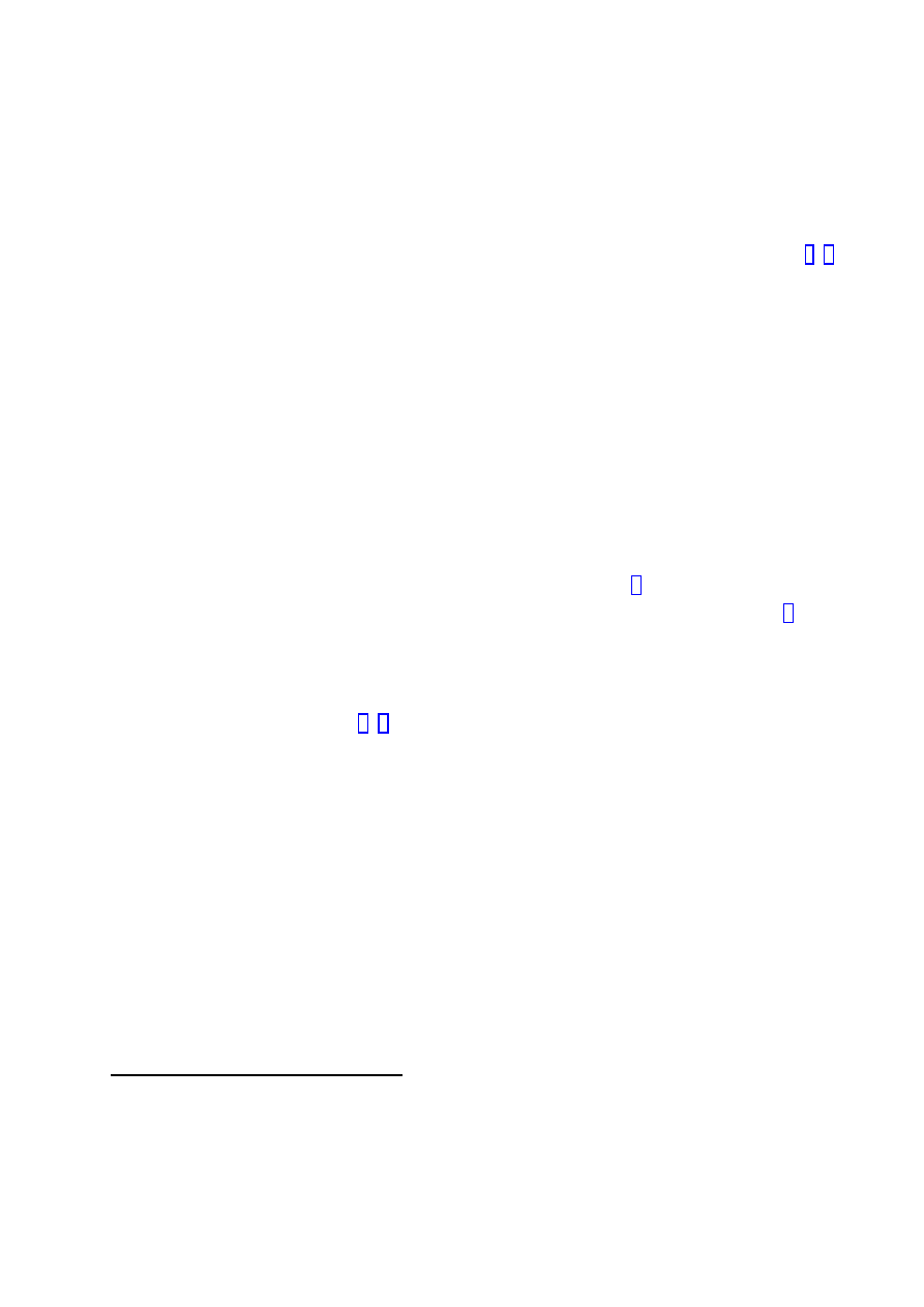
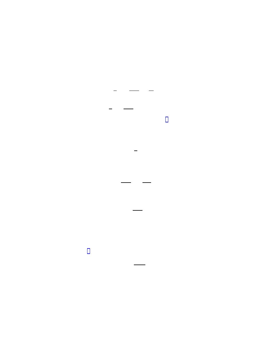
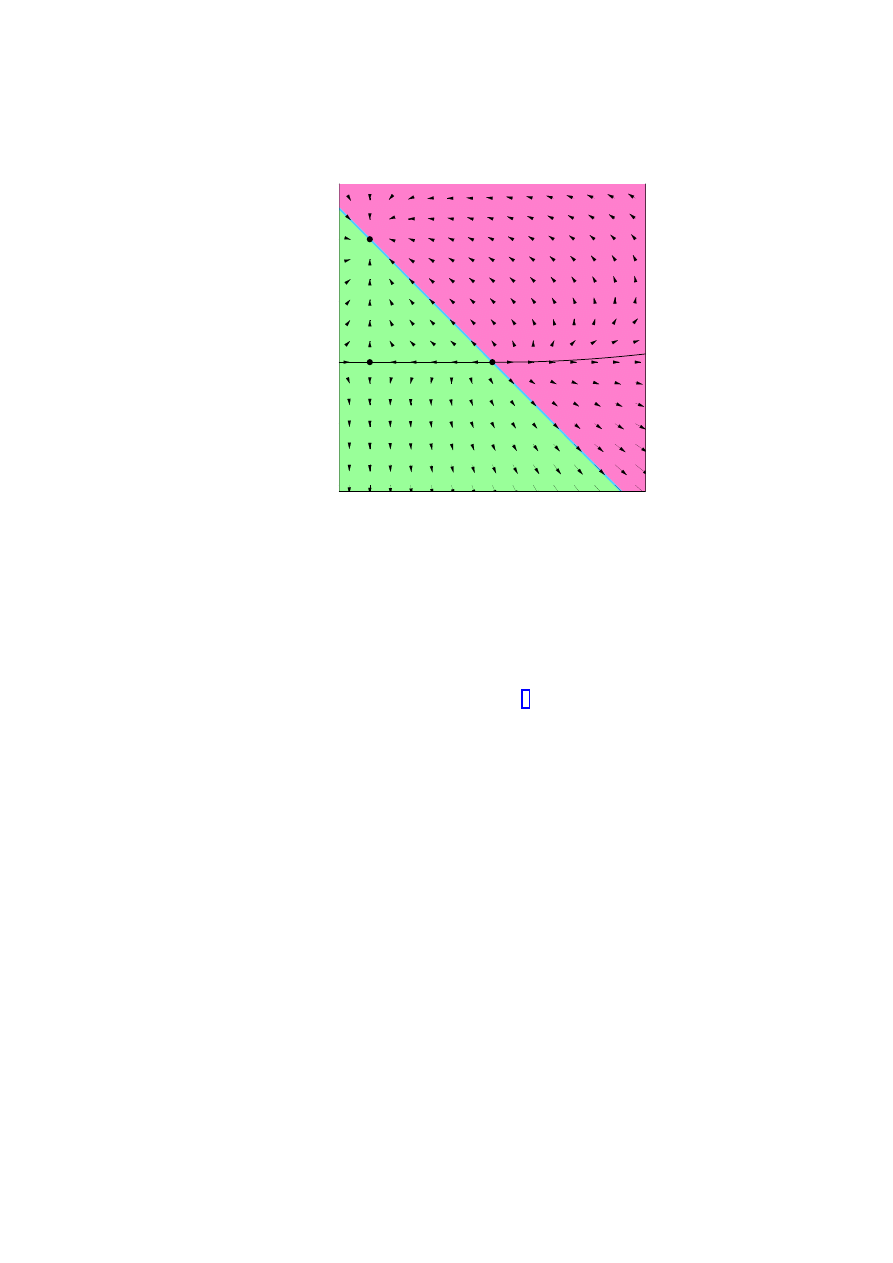
Figure 1: Dynamics of expanding universes dominated by matter and vacuum energy. The
arrows indicate the direction of evolution. Above and on the nearly-horizontal line are those
universes which expand forever, while those below will eventually recollapse.
Note that Ω
i
/Ω
j
= ρ
i
/ρ
j
= a
−(n
i
−n
j
)
, so the relative amounts of energy in different com-
ponents will change as the universe evolves. Figure 1 shows how Ω
M
and Ω
Λ
evolve in a
universe dominated by matter and a cosmological constant. Note that the only attractive
fixed point on the diagram is (Ω
M
= 0, Ω
Λ
= 1). In a sense this point represents the only
natural stable solution for cosmology, and one of the outstanding problems is why we don’t
find ourselves living there.
2.2
Exact solutions
Our actual universe consists of a complicated stew of radiation, matter, and vacuum energy,
as will be discussed below. It is nevertheless useful to consider exact solutions in order to
develop some intuition for cosmological dynamics. The simplest solutions are those for flat
universes, those with k = 0. For flat universes it is often more convenient to use Cartesian
coordinates on spacelike hypersurfaces, so that the metric takes the form
ds
2
=
−dt
2
+ a
2
(t)[dx
2
+ dy
2
+ dz
2
] ,
(14)
7
rather than the polar coordinates in (1). However, the solutions for a(t) are the same. In a
flat universe dominated by a single energy density source, the scaling of the source is directly
related to the expansion history:
k = 0, ρ
∝ a
−n
→ a ∝ t
2/n
.
(15)
(For n = 0, we get exponential growth.) Thus, a matter-dominated flat universe expands as
a
∝ t
2/3
, and a radiation-dominated flat universe as a
∝ t
1/2
. When k
6= 0, the solutions for
matter- and radiation-dominated universes are slightly more complicated, but may still be
expressed in closed form [22, 23]. (Even when k
6= 0, the curvature term −k/a
2
in the Fried-
mann equation will be subdominant to the energy density for very small a, so it is sensible
to model the early universe using the k = 0 metric.) When the energy density consists solely
of matter and/or radiation (or more generally when the energy density diminishes at least as
rapidly as a
−2
), negatively curved universes expand forever, while positively curved universes
eventually recollapse. An interesting special case occurs for ρ = 0, an empty universe, which
from (7) implies k =
−1. The solution is then linear expansion, a ∝ t; this is sometimes
called the “Milne universe”. In fact the curvature tensor vanishes in this spacetime, and it is
simply an unconventional coordinate system which covers a subset of Minkowski spacetime.
Let us now consider universes with a nonvanishing vacuum energy, with all other energy
set to zero. Unlike ordinary energy, a cosmological constant Λ = 8πGρ
Λ
can be either
positive or negative. When Λ > 0, we can find solutions for any spatial curvature:
k =
−1 →
a
∝ sinh
h
(Λ/3)
1/2
t
i
k = 0
→
a
∝ exp
h
(Λ/3)
1/2
t
i
k = +1
→ a ∝ cosh
h
(Λ/3)
1/2
t
i
.
(16)
In fact, all of these solutions are the same spacetime, “de Sitter space”, just expressed
in different coordinates. Any given spacetime can (locally) be foliated into spacelike hy-
persurfaces in infinitely many ways, although typically such hypersurfaces will be wildly
inhomogeneous; de Sitter space has the property that it admits Robertson-Walker foliations
with any of the three spatial geometries (just as Minkowski space can be foliated either by
surfaces of constant negative curvature to obtain the Milne universe, or more convention-
ally by flat hypersurfaces). In general such foliations will not cover the entire spacetime:
the k = +1 coordinates cover all of de Sitter (which has global topology R
× S
3
), while
the others do not. However, this doesn’t imply that the k = +1 RW metric is a “better”
representation of de Sitter. For different purposes, it might be useful to model a patch of
8
some spacetime by a patch of de Sitter in certain coordinates. For example, if our universe
went through an early phase in which it was dominated by a large positive vacuum energy
(as in the inflationary scenario, discussed below), but containing some trace test particles,
it would be natural to choose a coordinate system in which the particles were comoving
(traveling on worldlines orthogonal to hypersurfaces of constant time), which might be the
flat or negatively-curved representations. See Hawking and Ellis [22] for a discussion of the
connections between different coordinate systems.
When Λ < 0, equation (7) implies that the universe must have k =
−1. For this case the
solution is
a
∝ sin
h
(
−Λ/3)
1/2
t
i
.
(17)
This universe is known as “anti-de Sitter space”, or “AdS” for short. The RW coordinates
describe an open universe which expands from a Big Bang, reaches a maximum value of the
scale factor, and recontracts to a Big Crunch (recall that for a nonzero Λ the traditional
relationship between spatial curvature and temporal evolution does not hold). Again, how-
ever, these coordinates do not cover the entire spacetime (which has global topology R
4
).
There are a number of different coordinates that are useful on AdS, and they have been
much explored by string theorists in the context of the celebrated correspondence between
string theory on AdS in n dimensions and conformal field theory in n
− 1 dimensions; see
[24] for a discussion. One of the reasons why AdS plays a featured role in string theory is
that unbroken supersymmetry implies that the cosmological constant is either negative or
zero (see [25, 26] and references therein). Of course, in our low-energy world supersymmetry
is broken if it exists at all, and SUSY breaking generally contributes a positive vacuum en-
ergy, so one might think that it is not so surprising that we observe a positive cosmological
constant (see below). The surprise is more quantitative; the scale of SUSY breaking is at
least 10
3
GeV, while that of the vacuum energy is 10
−12
GeV.
de Sitter and anti-de Sitter, along with Minkowski space, have the largest possible number
of isometries for a Lorentzian manifold of the appropriate dimension; they are therefore
known as “maximally symmetric” (and are the only such spacetimes). In an n-dimensional
maximally symmetric space, the Riemann tensor satisfies
R
µνρσ
=
1
n(n
− 1)
R(g
µρ
g
νσ
− g
µσ
g
νρ
) ,
(18)
where R is the Ricci scalar, which in this case is constant over the entire manifold. The
well-known symmetries of Minkowski space include the Lorentz group SO(n
− 1, 1) and the
translations R
4
, together known as the Poincar´e group. de Sitter space possesses an SO(n, 1)
9
symmetry, while AdS has an SO(n
− 1, 2) symmetry. All of these groups are of dimension
n(n + 1)/2. There is a sense in which the maximally symmetric solutions can be thought
of as “vacua” of general relativity. In the presence of dynamical matter and energy (or
gravitational waves), the solution will be non-vacuum, and possess less symmetry.
2.3
Matter
An inventory of the constituents comprising the actual universe is hampered somewhat
by the fact that they are not all equally visible. The first things we notice are galaxies:
collections of self-gravitating stars, gas, and dust. The light from distant galaxies is (almost
always) redshifted, and the apparent recession velocity depends (almost exactly) linearly on
distance: v = H
0
d, where we interpret the slope as the Hubble parameter at the present
epoch. (The “almost”s are inserted because galaxies are not perfectly comoving objects, but
have proper motions that lead to the conventional Doppler shifting; not to mention that at
sufficiently large distances the linear Hubble law will break down.) Measuring extragalactic
distances is notoriously tricky, but most current measurements of the Hubble constant are
consistent with H
0
= 60
− 80 km/sec/Mpc, where 1 Mpc = 10
6
parsecs = 3
× 10
24
cm [27].
In particle-physics units (¯
h = c = 1), this is H
0
∼ 10
−33
eV. It is convenient to express
the Hubble constant as H
0
= 100h km/sec/Mpc, where 0.6
≤ h ≤ 0.8. Note that, since
ρ
i
= 3H
2
0
Ω
i
/8πG, measurements of ρ
i
will often be expressed as measurements of Ω
i
h
2
. The
Hubble constant provides a rough measure of the scale of the universe, since the age of a
matter- or radiation-dominated universe is t
0
∼ H
−1
0
.
We find perhaps 10
11
stars in a typical galaxy. The total amount of luminous matter in
all the galaxies we see adds up to approximately Ω
lum
∼ 10
−3
. In fact, most of the baryons
are not in the form of stars, but in ionized gas; our best estimates of the total baryon density
yield Ω
B
∼ 2 × 10
−2
[28, 29]. But the dynamics of individual galaxies implies that there is
even more matter there, in “halos” [30]. The implied existence of “dark matter” is confirmed
by applying the virial theorem to clusters of galaxies, by looking at the temperature profiles
of clusters, by “weighing” clusters using gravitational lensing, and by the large-scale motions
of galaxies between clusters. The overall impression is of a matter density corresponding to
Ω
M
∼ 0.1 − 0.4 [31, 32, 27, 33, 26].
There are innumerable fascinating facts about the matter in the universe. First and
arguably foremost, it all seems to be matter and not antimatter [34]. If, for example, half
of the galaxies we observe were composed completely of antimatter, we would expect to
see copious γ-ray emission from proton-antiproton annihilation in the gas in between the
10
galaxies. Since it seems more natural to imagine initial conditions in which matter and
antimatter were present in equal abundances, it appears necessary to invoke a dynamical
mechanism to generate the observed asymmetry, as will be discussed briefly in section (3.6).
The relative abundances of various elements are also of interest. Heavy elements can
be produced in stars, but it is possible to deduce “primordial” abundances through careful
observation. Most of the primordial baryons in the universe are to be found in the form of
hydrogen, with about 25% helium-4 (by mass), between 10
−5
and 10
−4
in deuterium, about
10
−5
in helium-3, and 10
−10
in lithium. As discussed below, these abundances provide a
sensitive probe of early-universe cosmology [35, 36, 37].
Besides baryons and dark matter, galaxies also possess large-scale magnetic fields with
root-mean-square amplitudes of order 10
−6
Gauss [38, 39]. These fields may be the result of
dynamo amplification of small seed fields created early in the history of the galaxies, or they
may be relics of processes at work in the very early universe.
Finally, we have excellent evidence for the existence of black holes in galaxies. There
are black holes of several solar masses which are thought to be the end-products of the
lives of massive stars, as well as supermassive black holes (M
≥ 10
6
M
) at the centers
of galaxies [40, 41]. In astrophysical situations the electric charges of black holes will be
negligible compared to their mass, since any significant charge will be quickly neutralized
by absorbing oppositely charged particles from the surrounding plasma. They can, however,
have significant spin, and observations have tentatively indicated spin parameters a
≥ 0.95
(where a = 1.0 in an extremal Kerr black hole) [42].
2.4
Cosmic Microwave Background
Besides the matter (luminous and dark) found in the universe, we also observe diffuse photon
backgrounds [43]. These come in all wavelengths, but most of the photons are to be found in
a nearly isotropic background with a thermal spectrum at a temperature [44] of 2.73
◦
K —
the cosmic microwave background. Careful observation has failed to find any deviation from
a perfect blackbody curve; indeed, the CMB spectrum as measured by the COBE satellite
is the most precisely measured blackbody curve in all of physics.
Why does the spectrum have this form? Typically, blackbody radiation is emitted by sys-
tems in thermal equilibrium. Currently, the photon background is essentially non-interacting,
and there is no accurate sense in which the universe is in thermal equilibrium. However,
as the universe expands, individual photon frequencies redshift with ν
∝ 1/a, and a black-
body curve will be preserved, with temperature T
∝ 1/a. Since the universe is expanding
11
now, it used to be smaller, and the temperature correspondingly higher. At sufficiently high
temperatures the photons were frequently interacting; specifically, at temperatures above
approximately 13 eV, hydrogen was ionized, and the photons were coupled to charged par-
ticles. The moment when the temperature become low enough for hydrogen to be stable
(at a redshift of order 10
3
) the universe became transparent. This moment is known as
“recombination” or “decoupling”, and the CMB we see today is to a good approximation a
snapshot of the universe at this epoch
.
Today, there are 422 CMB photons per cubic centimeter, which leads to a density pa-
rameter Ω
CMB
∼ 5 × 10
−5
. If neutrinos are massless (or sufficiently light), a hypothetical
neutrino background should contribute an energy density comparable to that in photons.
We don’t know of any other significant source of energy density in radiation, so in the con-
temporary universe the radiation energy density is dominated by the matter energy density.
But of course they depend on the scale factor in different ways, such that Ω
M
/Ω
R
∝ a. Thus,
matter-radiation equality should have occurred at a redshift z
EQ
∼ 10
4
Ω
M
.
The source of most current interest in the CMB is the small but crucial temperature
anisotropies from point to point in the sky [45, 46, 47]. We typically decompose the temper-
ature fluctuations into spherical harmonics,
∆T
T
=
X
lm
a
lm
Y
lm
(θ, φ) ,
(19)
and express the amount of anisotropy at multipole moment l via the power spectrum,
C
l
=
h|a
lm
|
2
i .
(20)
Higher multipoles correspond to smaller angular separations on the sky, θ = 180
◦
/l.
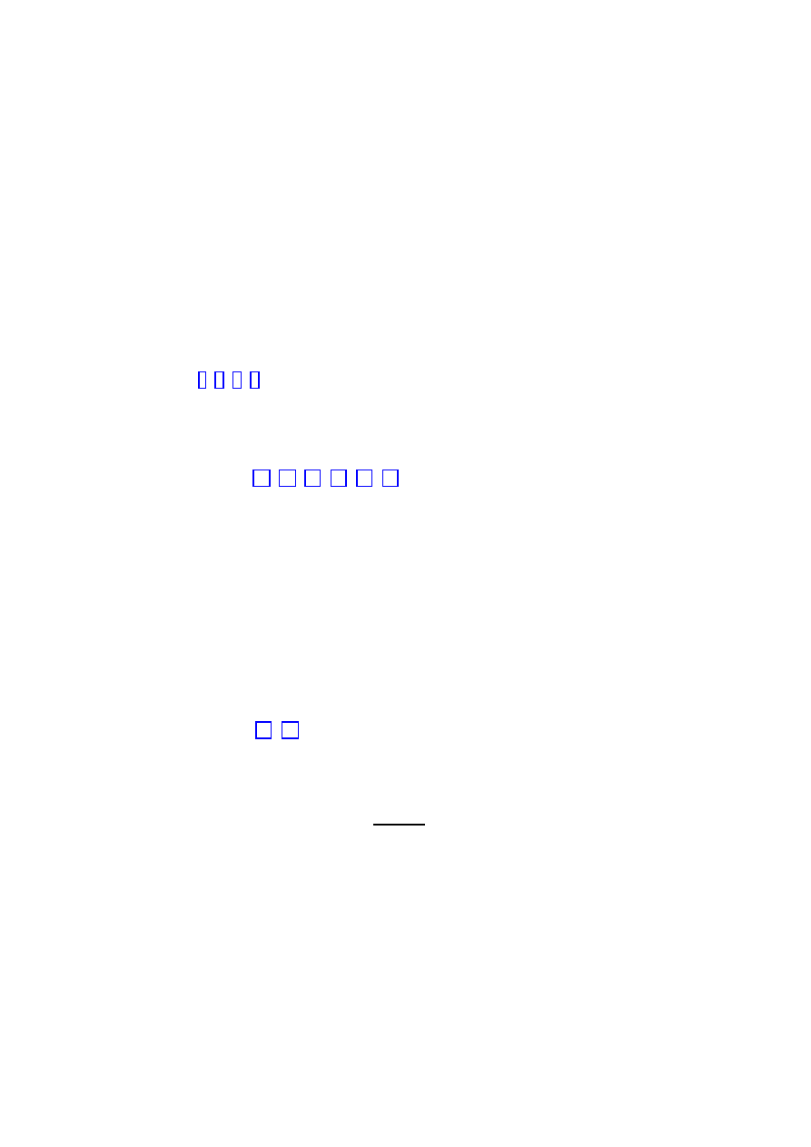
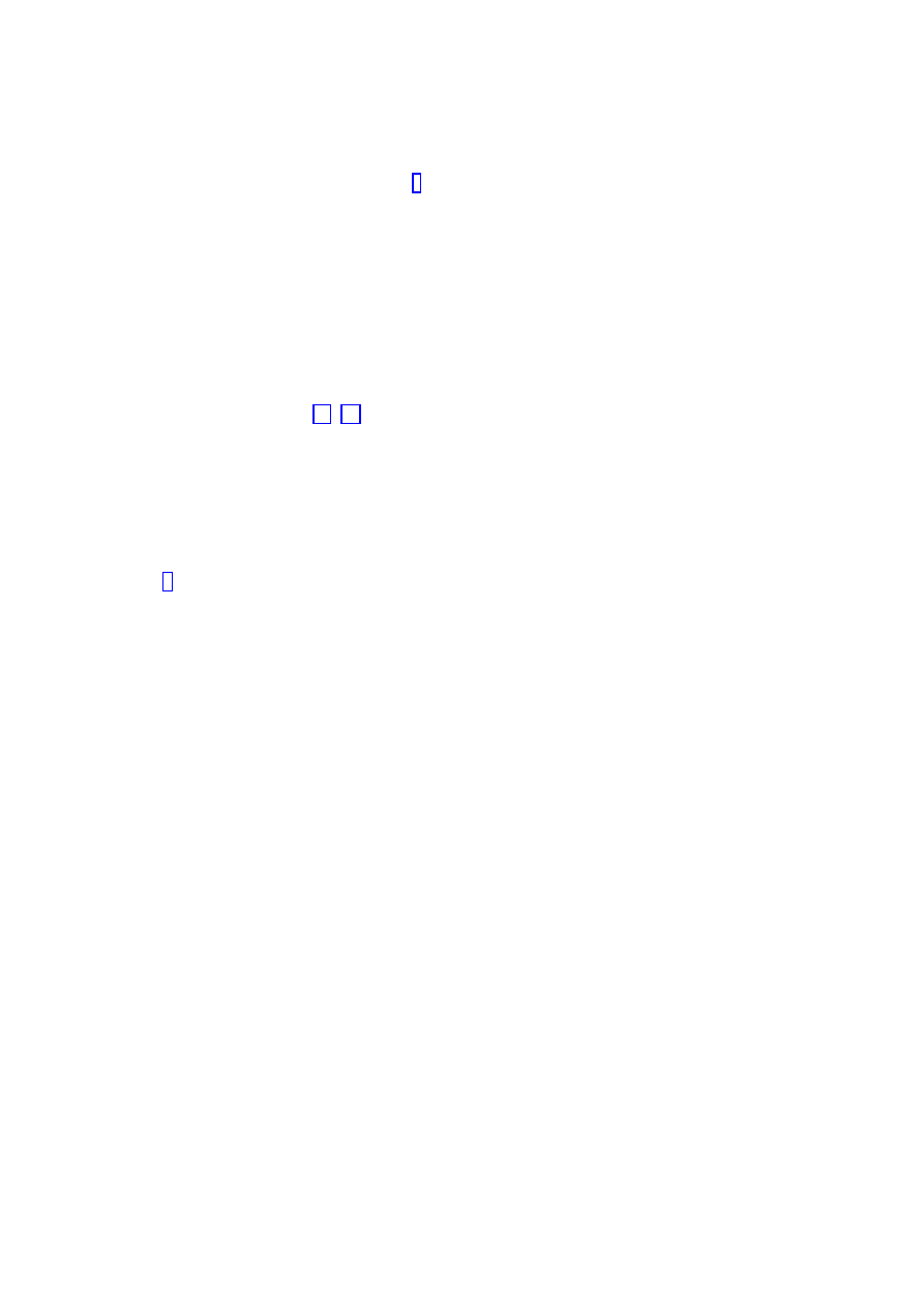
Figure 2 shows a summary of data as of summer 2000, with various experimental re-
sults consolidated into bins, along with a theoretical model. (See [48, 49, 50, 51] for some
recent observational work.) The curve shown in the figure is based on currently a specific
understanding of the primordial inhomogeneities, in which they are Gaussian fluctuations
of approximately equal magnitudes at all length scales (a “Harrison-Zeldovich spectrum”)
in a cold dark matter component, which are “adiabatic” in the sense that fluctuations in
the dark matter, photons, and baryons are all correlated with each other. A member of this
2
Occasionally a stickler will complain that “recombination” is a misnomer, since the electrons are combin-
ing with protons for the first time. Such people should be dealt with by pointing out that a typical electron
will combine and dissociate with a proton many times before finally settling down, so “re-” is a perfectly
appropriate prefix in describing the last of these combinations.
12
Figure 2: Amplitude of CMB temperature anisotropies, as a function of multipole moment l
(so that angular scale decreases from left to right). The data points are averaged from all of
the experiments performed as of Summer 2000. The curve is a theoretical model with scale-
free adiabatic scalar perturbations in a flat universe dominated by a cosmological constant.
Courtesy of Lloyd Knox.
family of models is characterized by cosmological parameters such as the Hubble constant,
the Ω
i
’s, and the amplitude of the initial fluctuations. A happy feature of these models is the
existence of “acoustic peaks” in the CMB spectrum, whose characteristics are closely tied to
the cosmological parameters. The first peak (the one at lowest l) corresponds to the angular
scale subtended by the Hubble radius H
−1
CMB
at recombination, which we can understand in
simple physical terms [45].
An overdense region of a given size R will contract under the influence of its own gravity,
which occurs over a timescale
∼ R (remember c = 1). For scales R H
−1
CMB
, overdense
regions will not have had time to collapse in the lifetime of the universe at last scattering. For
13
R
≤ H
−1
CMB
, protons and electrons will have had time to fall into the gravitational potential
wells, raising the temperature in the overdense regions (and lowering it in the underdense
ones). There will be a restoring force due to the increased photon pressure, leading to acoustic
oscillations which are damped by photon diffusion. The maximum amount of temperature
anisotropy occurs on the scale which has just had time to collapse but not equilibrate,
R
∼ H
−1
CMB
, which appears to us as a peak in the CMB anisotropy spectrum.
The angular scale at which we observe this peak is tied to the geometry of the universe:
in a negatively (positively) curved universe, photon paths diverge (converge), leading to a
larger (smaller) apparent angular size as compared to a flat universe [52, 53]. Although
the evolution of the scale factor also influences the observed angular scale, for reasonable
values of the parameters this effect cancels out and the location of the first peak will depend
primarily on the geometry. In a flat universe, we have
l
peak
∼ 200 ;
(21)
negative curvature moves the peak to higher l, and positive curvature to lower l. It is clear
from the figure that this is indeed the observed location of the peak; this result is the best
evidence we have that we live in a flat (k = 0, Ω = 1) Robertson-Walker universe.
More details about the spectrum (height of the peak, features of the secondary peaks)
will depend on other cosmological quantities, such as the Hubble constant and the baryon
density. Combined with constraints from other sources, data which will be gathered in
the near future from new satellite, balloon and ground-based experiments should provide a
wealth of information that will help pin down the parameters describing our universe. You
can calculate the theoretical curves at home yourself with the program CMBFAST [54]. The
CMB can also be used to constrain particle physics in various ways [46].
2.5
Evolution of the scale factor
Saul Perlmutter’s lectures at TASI-99 discussed the recent observations of Type Ia supernovae
as standard candles, and the surprising result that they seem to indicate an accelerating
universe and therefore a nonzero cosmological constant (or close relative thereof) [55, 56,
57, 58]. Since wonderfully entertaining reviews have recently become available [26], I will
not go into any detail here about this result and its consequences. The important point
is that the supernova results have received confirmation from a combination of dynamical
measurements of Ω
M
and the CMB constraints on Ω
tot
discussed in the previous section.
The favored universe is one with Ω
M
∼ 0.3 and Ω
Λ
∼ 0.7.
14
-30
-20
-10
0
10
0
0.5
1
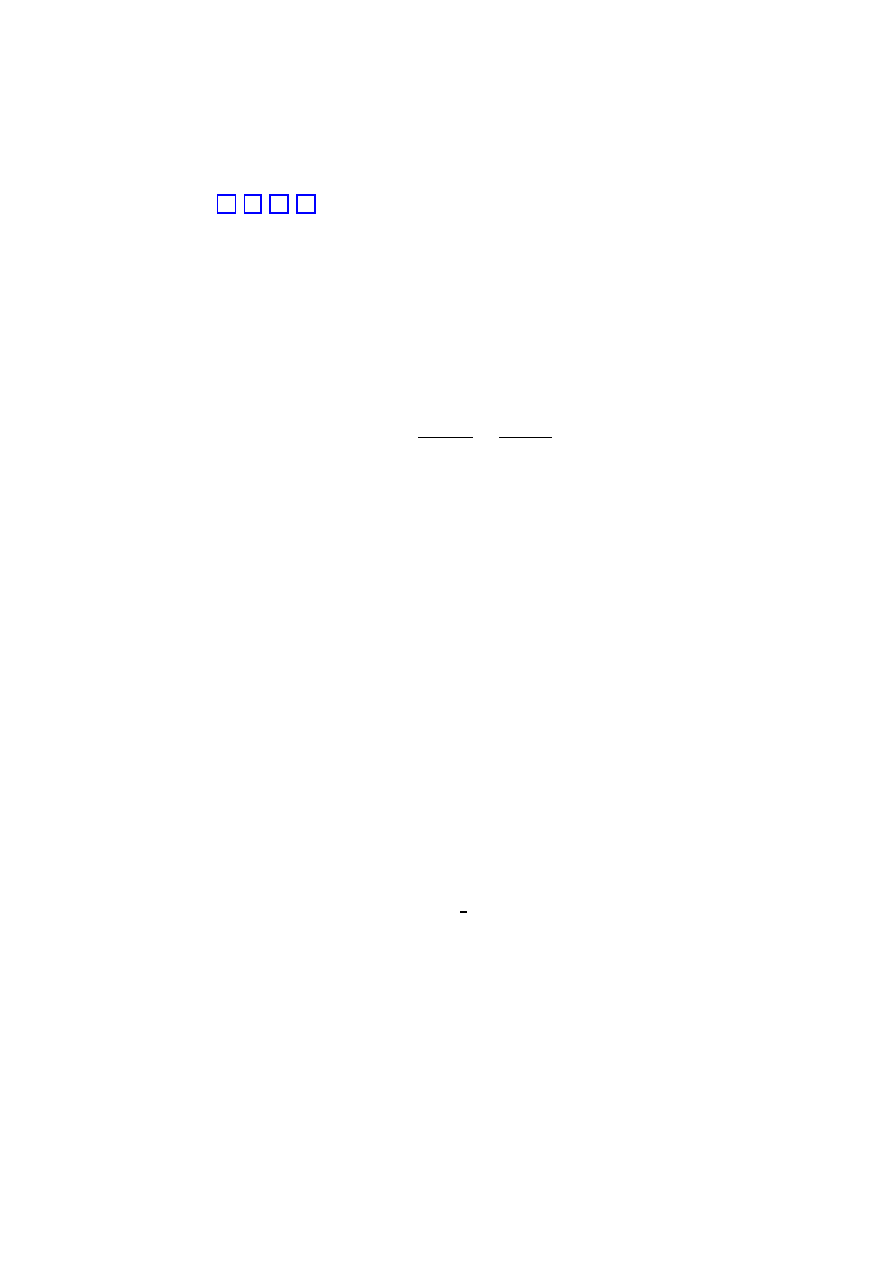
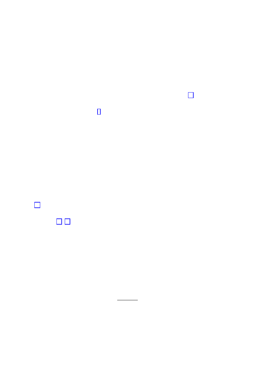
Figure 3: Evolution of the different density parameters in a universe with Ω
0,M
= 0.3,
Ω
0,Λ
= 0.7, and Ω
0,R
= 5
× 10
−5
.
If true, this is a remarkable universe, especially considering our early remark that the
different Ω
i
’s evolve at different rates. Figure 3 shows this evolution for the apparently-
favored universe, as a function of log(a). The period in which Ω
M
is of the same order as Ω
Λ
is a very brief one, cosmically speaking. It’s clearly crucial that we work to better understand
this remarkable result, which will have important consequences for both cosmology and
fundamental microphysics if it is eventually confirmed [59, 25, 26].
3
The youthful universe
15
3.1
Starting point
In the previous lecture we discussed the universe as we see it, as well as the dynamical equa-
tions which describe its evolution according to general relativity. One conclusion is that the
very early universe was much smaller and hotter than the universe today, and the energy
density was radiation-dominated. We also saw that the universe on large scales could be
accurately described by a perturbed Robertson-Walker metric. On thermodynamic grounds
(backed up by evidence from CMB anisotropy) it seems likely that these perturbations are
growing rather than shrinking with time, at least in the matter-dominated era; it would
require extreme fine-tuning of initial conditions to arrange for diminishing matter perturba-
tions [60]. Thus, the early universe was smoother as well.
Let us therefore trace the history of the universe as we reconstruct it given these con-
ditions plus our current best guesses at the relevant laws of physics. We can start at a
temperature close to but not quite at the reduced
Planck scale M
P
= 1/
√
8πG
∼ 10
18
GeV,
so that we can (hopefully) ignore string theory (!). We imagine an expanding universe with
matter and radiation in a thermal state, perfectly homogeneous and isotropic (we can put
in perturbations later), and all conserved quantum numbers set to zero (no chemical poten-
tials). Note that asymptotic freedom makes our task much easier; at the high temperatures
we are concerned with, QCD (and possible grand unified gauge interactions) are weakly
coupled, allowing us to work within the framework of perturbation theory.
3.2
Phase transitions
The high temperatures and densities characteristic of the early universe typically put matter
fields into different phases than they are in at zero temperature and density, and often these
phases are ones in which symmetries are restored [4, 5]. Consider a simple theory of a real
scalar field φ with a Z
2
symmetry φ
→ −φ. The potential at zero temperature might be of
the form
V (φ, T = 0) =
−
µ
2
2
φ
2
+
λ
4
φ
4
.
(22)
Interactions with a thermal background typically give positive contributions to the potential
at finite temperature:
V (φ, T ) = V (φ, 0) + αT
2
φ
2
+
· · · ,
(23)
3
The “ordinary” Planck scale is simply 1/
√
G
∼ 10
19
GeV. It is only an accident of history (Newton’s
law of gravity predating general relativity, or for that matter Poisson’s equation) that it is defined this way,
and the tradition is continued by those with a great fondness for typing “8
\pi”.
16
where α = λ/8 in the theory defined by (22).
At high T , the coefficient of φ
2
in the effective potential, (αT
2
−
1
2
µ
2
), will be a positive
number, so the minimum-energy state will be one with vanishing expectation value,
hφi = 0.
The Z
2
symmetry is unbroken in such a state. As the temperature declines, eventually the
coefficient will be negative and there will be two lowest-energy states, with equal and oppo-
site values of
hφi. A zero-temperature vacuum will be built upon one of these values, which
are not invariant under the Z
2
; we therefore say the symmetry is spontaneously broken.
The dynamics of the transition from unbroken to broken symmetry is described by a phase
transition, which might be either first-order or second-order. A first-order transition is one
in which first derivatives of the order parameter (in this case φ) are discontinuous; they
are generally dramatic, with phases coexisting simultaneously, and proceed by nucleation of
bubbles of the new phase. In a second-order transition only second derivatives are discontin-
uous; they are generally more gradual, without mixing of phases, and proceed by “spinodal
decomposition”. (I hope it is clear that a huge amount of honest physics is being glossed
over in this brief discussion.)
3.3
Topological defects
Note that, post-transition, the field falls into the vacuum manifold (the set of field values
with minimum energy — in our current example it’s simply two points) essentially randomly.
It will fall in different directions at different spatial locations x
1
and x
2
separated by more
than one correlation length of the field. In an ordinary FRW universe, the field cannot be
correlated on scales larger than approximately H
−1
, as this is the distance to the particle
horizon (as we will discuss below in the section on inflation). If
hφ(x
1
)
i = +v and hφ(x
2
)
i =
−v, then somewhere in between x
1
and x
2
φ must climb over the energy barrier to pass
through zero. Where this happens there will be energy density; this is known as a “topological
defect” (in this case a defect of codimension one, a domain wall). The argument that the
existence of horizons implies the production of defects is known as the “Kibble mechanism”.
More complicated vacuum manifolds
M will give other forms of defects, depending on
the topology of
M; if the homotopy group π
q
(
M) (the set of topologically inequivalent maps
from S
q
into
M) is nontrivial, we will have defects of (spatial) codimension (q + 1). In three
spatial dimensions, nontrivial π
0
(
M) gives rise to walls (such as in our example, for which
π
0
(
M) = Z
2
), nontrivial π
1
(
M) gives rise to (cosmic) strings, and nontrivial π
2
(
M) gives
rise to pointlike defects (monopoles) [61]. Nobody will be upset if you refer to these defects
as “branes”.
17
When a symmetry group G is broken to a subgroup H, the vacuum manifold is the
quotient space
M = G/H, so we can determine what sorts of defects might be created at an
early-universe phase transition. A good tool for doing this is the exact homotopy sequence
· · · → π
q+1
(G/H)
→ π
q
(H)
α
q
−→ π
q
(G)
β
q
−→ π
q
(G/H)
γ
q
−→ π
q
−1
(H)
→ · · · → π
0
(G/H)
→ 0 ,
(24)
where 0 is the trivial group. The maps α
i
, β
i
and γ
i
are specified in terms of the spaces
G, H and G/H, and they are all group homomorphisms. For example, the map α
q
takes
the image of a q-sphere in H into an image of a q-sphere in G using the inclusion of H as
a subgroup in G, i : H ,
→ G. “Exactness” means that the image of each map is precisely
equal to the kernel (the set of elements taken to zero) of the map following it.
An important consequence of exactness is that if two spaces A and B are sandwiched
between the trivial group, 0
→ A
ω
−→ B → 0, then the map ω must be an isomorphism.
This is easy to see: since the kernel of B
→ 0 is all of B, ω must be onto. Meanwhile, since
the kernel of ω is the image of 0
→ A (which is just zero), in order for ω to be a group
homomorphism it must be one-to-one. Thus, ω is an isomorphism. You can also check for
yourself that the exact sequence 0
→ A → 0 implies that A must be the trivial group.
The exact homotopy sequence can be used in conjunction with our knowledge of various
facts about the topology of Lie groups to calculate π
q
(
M). Some of the relevant facts
include: 1.) For any Lie group G, π
2
(G) = 0. 2.) For any simple group G, π
3
(G) = Z.
3.) π
1
(SU(n)) = 0, but π
1
(U(n)) = Z, and π
1
(SO(n > 2)) = Z
2
. 4.) π
0
simply counts
the number of disconnected pieces into which a space falls, so π
0
(SU(n)) = π
0
(SO(n)) =
π
0
(U(n)) = 0, and π
0
(O(n)) = Z
2
. 5.) Finally, for any spaces (not just groups) A and B,
we have π
q
(A
× B) = π
q
(A)
× π
q
(B). For some examples of homotopy calculations see [63].
As an example, consider SU(2) breaking down to U(1). In the exact homotopy sequence,
π
0
(SU(2)/U(1)) and π
1
(SU(2)/U(1)) are each sandwiched between 0’s, so both are trivial.
On the other hand, we have
π
2
(SU(2)) = 0
→ π
2
(SU(2)/U(1))
→ π
1
(U(1)) = Z
→ π
1
(SU(2)) = 0 ,
(25)
so the map π
2
(SU(2)/U(1))
→ Z must be an isomorphism, π
2
(SU(2)/U(1)) = Z. This
theory (the “Georgi-Glashow model”) therefore predicts magnetic monopoles with charges
(proportional to the winding number of the map S
2
→ SU(2)/U(1)) taking values in Z. [The
modifier “magnetic” is only appropriate if the original SU(2) was a gauge symmetry, in which
case the monopole acts as a source for the magnetic field of the unbroken U(1). There can
18
also be monopoles from the breakdown of a global symmetry, although there are no solutions
with finite energy. Infinite energies aren’t generally looked down upon by cosmologists, as
the universe is a big place; more of a worry would be an infinite energy density, which does
not occur in global monopoles.]
Once defects are produced at a phase transition, the question of cosmological interest is
how they subsequently evolve. This will be very different for different sorts of defects, and
can be altered by going beyond the simplest models [61]. We will encounter some examples
below.
3.4
Relic particle abundances
One of the most useful things to do in cosmology is to calculate the abundance of a given
particle species from a specified initial condition in the early universe. First consider the
properties of particles in thermal equilibrium (with zero chemical potential). In the rela-
tivistic limit m
T , the number density n and energy density ρ are given by
n
≈ T
3
ρ
≈ T
4
.
(26)
Here we have begun what will be a conventional practice during this lecture, ignoring factors
of order unity. To get them right see any standard text [3, 4]. Note that the Friedmann
equation during a phase when the universe is flat and radiation-dominated can be expressed
simply as
H
≈
T
2
M
P
.
(27)
(The appearance of the Planck scale here isn’t a sign of the importance of quantum gravity,
but merely classical gravity plus the fact that we’ve set ¯
h = c = 1.) In the nonrelativistic
limit (m
T ), meanwhile, we have
n
≈ (mT )
3/2
e
−m/T
ρ
≈ mn .
(28)
The energy density of nonrelativistic particles is just their number density times the indi-
vidual particle masses.
Particles will tend to stay in thermal equilibrium as long as reaction rates Γ are much
faster than the expansion rate H, so that the particles have plenty of time to interact before
the expansion of the universe separates them. A particle for which Γ
H is referred
19
to as decoupled or “frozen-out”; for species which are kept in thermal equilibrium by the
exchange of massive bosons, Γ
∝ T
5
, and such particles will be frozen-out at sufficiently
low temperatures. (Of course, a species may be noninteracting with the thermal bath and
nevertheless in an essentially thermal distribution, as we’ve already noted for the CMB; as
another example, massless neutrinos decouple while in a thermal distribution, which is then
simply preserved as the universe expands and the temperature decreases.)
There are two limiting cases of interest, decoupling while relativistic (“hot relics”) and
while nonrelativistic (“cold relics”)
. A hot relic X will have a number density at freeze-out
approximately equal to the photon number density,
n
X
(T
f
)
∼ T
3
f
∼ n
γ
(T
f
) ,
(29)
where T
f
is the freeze-out temperature. Subsequently, the number densities of both X and
photons simply diminish as the volume increases, n
X
∝ n
γ
∝ a
−3
, so their present-day
number density is approximately
n
X0
∼ n
γ0
∼ 10
2
cm
−3
.
(30)
We express this number as 10
2
rather than 422 since the roughness of our estimate does not
warrant such misleading precision. The leading correction to this value is typically due to
the production of additional photons subsequent to the decoupling of X; in the Standard
Model, the number density of photons increases by a factor of approximately 100 between
the electroweak phase transition and today, and a species which decouples during this period
will be diluted by a factor of between 1 and 100 depending on precisely when it freezes out.
So, for example, neutrinos which are light (m
ν
< MeV) have a number density today of
n
ν
= 115 cm
−3
per species, and a corresponding contribution to the density parameter (if
they are nevertheless heavy enough to be nonrelativistic today) of
Ω
0,ν
=
m
ν
92 eV
h
−2
.
(31)
Thus, a neutrino with m
ν
∼ 10
−2
eV (as might be a reasonable reading of the recent
SuperKamiokande data [64]) would contribute Ω
ν
∼ 2 × 10
−4
. This is large enough to
be interesting without being large enough to make neutrinos be the dark matter. That’s
good news, since the large velocities of neutrinos make them free-stream out of overdense
regions, diminishing primordial perturbations and leaving us with a universe which has much
4
“Hot dark matter”, then, refers to dark matter particles which were relativistic when they decoupled —
not necessarily relativistic today.
20
less structure on small scales than we actually observe. On the other hand, the roughness
of our estimates (and the data) leaves open the possibility that neutrinos are nevertheless
dynamically important, perhaps as part of a complicated mixture of dark matter particles
For cold relics, the number density is plummeting rapidly during freeze-out due to the
exponential in (28), and the details of the interactions can be important. But, very roughly,
the answer works out to be
n
X
∼
n
γ
σ
0
m
X
M
P
,
(32)
where σ
0
is the annihilation cross-section of X at T = m
X
. An example of a cold relic is
provided by protons, for which m
p
∼ 1 GeV and σ
0
∼ m
−2
π
∼ (.1 GeV)
−2
. This implies
n
p
/n
γ
∼ 10
−20
, which is rather at odds with the observed value n
p
/n
γ
∼ 10
−10
; this conflict
brings home the need for a sensible theory of baryogenesis [66, 67, 68]. (We might worry
that the disagreement between theory and observation in this case indicates that we had no
clue how to really calculate relic abundances, if it weren’t for the shining counterexample of
nucleosynthesis to be discussed below.)
A less depressing example of a cold relic is provided by weakly interacting massive par-
ticles (“wimps”), a generic name given to particles with cross-sections characteristic of the
weak interactions, σ
0
∼ G
F
∼ (300 GeV)
−2
. Then the relic abundance today will be
n
0,wimp
∼
n
γ0
G
F
m
wimp
M
P
∼
10
−13
GeV
m
wimp
!
cm
−3
,
(33)
which leads in turn to a density parameter
Ω
0,wimp
∼ 1 .
(34)
The independence of (34) on m
wimp
(at least at our crude level of approximation) means
that particles with weak-interaction annihilation cross-sections provide excellent candidates
for cold dark matter. A standard example is the lightest supersymmetric particle (“LSP”)
3.5
Vacuum displacement
Another important possibility is the existence of relics which were never in thermal equilib-
rium. An example of these has already been discussed: the production of topological defects
at phase transitions. Let’s discuss another kind of non-thermal relic, which derives from
21
what we might call “vacuum displacement”. Consider the action for a real scalar field in
curved spacetime (assumed to be four-dimensional):
S =
Z
d
4
x
√
−g
−
1
2
g
µν
∂
µ
φ∂
ν
φ
− V (φ)
.
(35)
If we assume that φ is spatially homogeneous (∂
i
φ = 0), its equation of motion in the
Robertson-Walker metric (1) will be
¨
φ + 3H ˙
φ + V
0
(φ) = 0 ,
(36)
where an overdot indicates a partial derivative with respect to time, and a prime indicates
a derivative with respect to φ. For a free massive scalar field, V (φ) =
1
2
m
2
φ
φ
2
, and (36)
describes a harmonic oscillator with a time-dependent damping term. For H > m
φ
the field
will be overdamped, and stay essentially constant at whatever point in the potential it finds
itself. So let us imagine that at some time in the very early universe (when H was large) we
had such an overdamped homogeneous scalar field, stuck at a value φ = φ
∗
; the total energy
density in the field is simply the potential energy
1
2
m
2
φ
φ
2
∗
. The Hubble parameter H will
decrease to approximately m
φ
when the temperature reaches T
∗
=
q
m
φ
M
P
, after which the
field will be able to evolve and will begin to oscillate in its potential. The vacuum energy
is converted to a combination of vacuum and kinetic energy which will redshift like matter,
as ρ
φ
∝ a
−3
; in a particle interpretation, the field is a Bose condensate of zero-momentum
particles. We will therefore have
ρ
φ
(a)
∼
1
2
m
2
φ
φ
2
∗
a
∗
a
3
,
(37)
which leads to a density parameter today
Ω
0,φ
∼
φ
4
∗
m
φ
10
−19
GeV
5
!
1/2
.
(38)
A classic example of a non-thermal relic produced by vacuum displacement is the QCD
axion, which has a typical primordial value
hφi ∼ f
PQ
and a mass m
φ
∼ Λ
2
QCD
/f
PQ
, where
f
PQ
is the Peccei-Quinn symmetry-breaking scale and Λ
QCD
∼ 0.3 GeV is the QCD scale [4].
In this case, plugging in numbers reveals
Ω
0,φ
∼
f
PQ
10
13
GeV
!
3/2
.
(39)
The Peccei-Quinn scale is essentially a free parameter from a theoretical point of view,
but experiments and astrophysical constraints have ruled out most values except for a small
22
window around f
PQ
∼ 10
12
GeV. The axion therefore remains a viable dark matter candidate
[69, 70]. Note that, even though dark matter axions are very light (Λ
2
QCD
/f
PQ
∼ 10
−4
eV),
they are extremely non-relativistic, which can be traced to the non-thermal nature of their
production process. (Another important way to produce axions is through the decay of axion
cosmic strings [4, 61].)
3.6
Thermal history of the universe
We are now empowered to take a brief tour through the evolution of the universe, starting
at a temperature T
∼ 10
16
GeV, and assuming the correctness of the Standard Model plus
perhaps some grand unified theory, but nothing truly exotic. (At temperatures higher than
this, not only do we have to worry about quantum gravity, but the Hubble parameter is so
large that essentially no perturbative interactions are able to maintain thermal equilibrium;
either strong interactions are important, or every species is frozen out.) The first event we
encounter as the universe expands is the grand unification phase transition (if there is one).
Here, some grand unified group G breaks to the standard model group
[SU(3)
× SU(2) ×
U(1)]/Z
6
, with popular choices for G including SU(5), SO(10), and E
6
.
Most interesting particles decay away after the GUT transition, with the possible excep-
tion of the all-important baryon asymmetry. As Sakharov long ago figured out, to make a
baryon asymmetry we need three conditions [66, 67, 68]:
1. Baryon number violation.
2. C and CP violation.
3. Departure from thermal equilibrium.
The X-bosons of GUTs typically have decays which can violate B, C, and CP . Departure
from equilibrium happens because the X’s first freeze out, then decay. With the right choice
of parameters, we can get n
B
/n
γ
∼ 10
−10
, the sought-after number.
One problem with this scenario is that, at T > T
EW
, nonperturbative effects in the
standard model (sphalerons) can violate baryon number. These will tend to restore the
baryon number to its equilibrium value (zero). A potential escape is to notice that sphalerons
5
You will often hear it said that the standard model gauge group is SU(3)
× SU(2) × U(1), but this is not
strictly correct; there is a Z
6
subgroup leaving all of the standard-model fields invariant. The Lie algebras
of the two groups are identical, which is usually all that particle physicists care about, but when topology is
important it is safer to keep track of the global structure of the group.
23
violate B and lepton number L but preserve the combination B
− L, so that for every excess
baryon produced a corresponding lepton must be produced. If our GUT generates a nonzero
B
− L it will therefore survive, as it cannot be changed by standard model processes. The
SU(5) theory conserves B
− L and is therefore apparently not the origin of the baryon
asymmetry, although B
− L can be generated in SO(10) models [67, 68].
Another worry about GUTs is the prediction of magnetic monopoles. Since π
1
(G) = 0
for any simple Lie group G, we have π
2
(G/H) = π
1
([SU(3)
× SU(2) × U(1)]/Z
6
) = Z, and
monopoles are inescapable. We end up with
Ω
0,mono
∼ 10
11
T
GUT
10
14
GeV
3
m
mono
10
16
GeV
.
(40)
This is far too big; the monopole abundance in GUTs is a serious problem, one which can
be solved by inflation (which we will discuss later).
Depending on the details of the symmetry group being broken, the GUT phase transition
can also produce domain walls (which also disastrously overdominate the universe) or cosmic
strings (which will not dominate the energy density, and in fact may have various beneficial
effects) [61].
Below the GUT temperature, nothing really happens (as far as we know) until T
EW
∼
300 GeV (z
∼ 10
15
), when the Standard Model gauge symmetry [SU(3)
× SU(2) × U(1)]/Z
6
is broken to SU(3)
× U(1). No topological defects are produced. (Magnetic fields may be,
however; see for example [71, 72, 73].) Most interestingly, the electroweak phase transition
may be responsible for baryogenesis [66, 67, 68]. The nonperturbative B-violating inter-
actions of the Standard Model are exponentially suppressed after the phase transition, so
any asymmetry generated at that time will be preserved. The important question is the
amount of CP violation and departure from thermal equilibrium. Both exist in the minimal
Standard Model; CP violation is present in the CKM matrix, and expansion of the universe
provides some departure from equilibrium. Both are very small, however; the amounts are
apparently not nearly enough to generate the required asymmetry.
It is therefore necessary to augment the Standard Model. Fortunately the simple action
of adding additional Higgs bosons can work both to increase the amount of CP violation (by
introducing new mixing angles) and the departure from thermal equilibrium (by changing
the phase transition from second order, which it is in the SM for experimentally allowed
values of the Higgs mass, to first order). Supersymmetric extensions of the SM require an
extra Higgs doublet in addition to the one of the minimal SM, so there is some hope for a
SUSY scenario. At this point, however, the relevant dynamics at the phase transition are
24
not sufficiently well understood for us to say whether electroweak baryogenesis is a sensible
idea. (It does, however, have the pleasant aspect of being related to experimentally testable
aspects of particle physics.)
There is one more scenario worth mentioning, known as Affleck-Dine baryogenesis [74, 66].
The idea here is to have a scalar condensate with energy density produced by vacuum
displacement, but to have the scalar carry baryon number. Its decay can then lead to the
observed baryon asymmetry.
After the electroweak transition, the next interesting event is the QCD phase transition at
T
QCD
∼ 0.3 GeV. Actually there are two things that happen, lumped together for convenience
as the “QCD phase transition”: chiral symmetry breaking, and the confinement of quarks
and gluons into hadrons. Our understanding of the QCD transition is also underdeveloped,
although it is likely to be second order and does not lead to any important relics [75].
At a temperature of T
f
∼ 1 MeV, the weak interactions freeze out, and free neutrons
and protons decouple. The neutron to proton ratio at this time is approximately 1/6, and
gradually decreases as the neutrons decay. Soon thereafter, at around T
BBN
∼ 80 keV, almost
all of the neutrons fuse with protons into light elements (D,
3
He,
4
He, Li), a process known
as “Big Bang Nucleosynthesis” [35, 37, 36]. Although it would seem to be a rather mundane
low-energy phenomenon from the lofty point of view of constructing a theory of everything,
the results of BBN are actually of great importance to string theory (or any other theories
which could affect cosmology), since they offer by far the best empirical constraints on the
behavior of the universe at relatively early times.
The abundances of light elements, like those of any other relics, depend on the interplay
between interaction rates Γ
i
of species i and the Hubble parameter H. The reaction rates
depend in turn on the baryon to photon ratio n
B
/n
γ
, not to mention the parameters of the
Standard Model (the fine-structure constant α, the Fermi constant G
F
, the electron mass
m
e
, etc.). Since BBN occurs well into the radiation-dominated era, the expansion rate is
H
2
=
1
3M
2
P
ρ
R
.
(41)
In the standard picture, ρ
R
comes essentially from photons (whose density we can count) and
neutrinos (whose density per species we have calculated above), as well as electrons when
T > m
e
.
It is a remarkable fact that the observed light-element abundances, coupled with the
observed number of light neutrino species N
ν
= 3, are consistent with the BBN prediction
for n
B
/n
γ
≈ 5 × 10
−10
, a number which is consistent with the observed ratio of baryons to
25
photons. (Consistent in the sense of being not incompatible; in fact the observed number
of baryons is somewhat lower, but there’s nothing stopping some of the baryons from being
dark [29].) The agreement, furthermore, is not with a single number, but the individual
abundances of D,
4
He, and
7
Li. Not only does this give us confidence in our ability to
calculate relic abundances (both of nuclei and of the neutrinos that enter the calculation),
it also implies that the current values of n
B
/n
γ
, the number density of hot relics, Newton’s
constant G, the fine structure constant α, and all of the other parameters of physics that
enter the calculation, are similar to what their values were at the time of BBN, when the
universe was only 1 second old [76]. This is astonishing when we consider the number of
ways in which they could have varied, as discussed briefly in the next section [77].
Apart from constraints on specific models, nucleosynthesis also provides the best evidence
that the early universe was in a hot thermal state, with dynamics governed by the conven-
tional Friedmann equation. Although it is possible to imagine alternative early histories
which are compatible with the observed light-element abundances, it would be surprising if
any dramatically different model led coincidentally to the same predictions as the conven-
tional picture.
3.7
Gravitinos and moduli
An example of a model constrained by BBN is provided by any theory of supergravity in
which SUSY is broken at an intermediate scale M
I
∼ 10
11
GeV in a hidden sector (the
gravitationally mediated models). In these theories the gravitino, the superpartner of the
graviton, will have a mass
m
3/2
∼ M
2
I
/M
P
∼ 10
3
GeV
(42)
(which is also the scale of SUSY breaking in the visible sector). The gravitino is of special
interest since its interactions are so weak (its couplings, gravitational in origin, are suppressed
by powers of M
P
) implying that 1.) it decouples early, while relativistic, leaving a large relic
abundance, and 2.) it decays slowly and therefore relatively late. Indeed, the lifetime is
τ
3/2
∼ M
2
P
/m
3
3/2
∼ 10
27
GeV
−1
∼ 10
3
sec ,
(43)
somewhat after nucleosynthesis. The decaying gravitinos produce a large number of high-
energy photons, which can both dilute the baryons and photodissociate the nuclei, changing
their abundances and thereby ruining the agreement with observation. This “gravitino prob-
lem” might be alleviated by inflation (as we will later discuss), but serves as an important
constraint on specific models [78, 79, 80, 81, 82].
26
The success of BBN also places limits on the time variation of the coupling constants
of the Standard Model
. In string theory, these couplings are all related to the expectation
values of moduli (scalar fields parameterizing “flat directions” in field space which arise due
to the constraints of supersymmetry), and could in principle vary with time [83]. The fact
that they don’t vary is most easily accommodated by imagining that the moduli are sitting at
the minima of some potentials; in fact this is completely sensible given that supersymmetry
is broken, so we expect that m
moduli
∼ M
SUSY
∼ 10
3
GeV, enough to fix their values for all
temperatures less than T
∼
√
M
SUSY
M
P
∼ 10
11
GeV (although at higher temperatures they
could vary in interesting ways).
On the other hand, massive moduli present their own problems. They are produced as
non-thermal relics due to vacuum displacement [86, 87, 88]. At high temperatures the fields
are at some random point in moduli space, which will typically be of order φ
∗
∼ M
P
. If
the moduli were stable, from (39) we would therefore expect a contribution to the critical
density of order
Ω
0,moduli
∼ 10
27
.
(44)
This number is clearly embarrassingly big, and something has to be done about it. The
moduli can of course decay into other particles, but their lifetimes are similar to those of
gravitinos, and their decay also tends to destroy the success of BBN. Due to their different
production mechanism, it is harder to dilute the moduli abundance during inflation (since
the scalar vev can remain displaced while inflation occurs), and the “moduli problem” poses
a significant puzzle for string theories. (One promising solution would be the existence of a
point of enhanced symmetry which would make the high-temperature and low-temperature
minima of the potential coincide [89].)
In addition to the overproduction of moduli, there are also problems with their stabi-
lization, especially for the dilaton, perhaps the best-understood example of a modulus field.
One problem is that the dilaton expectation value acts as a coupling constant in string the-
ory, and very general arguments indicate that the dilaton cannot be stabilized at a value we
would characterize as corresponding to weak coupling [90]. Another is that, in certain popu-
lar models for stabilizing the dilaton using gaugino condensates, the cosmological evolution
would almost inevitably tend to overshoot the desired minumum of the dilaton potential and
run off to an anti-de Sitter vacuum [91]. Problems such as these are the subject of current
6
Note that there are a number of other constraints on such time dependence, including solar-system tests
of gravity, the relative spacing of absorption lines in quasar spectra, and isotopic abundances in the Oklo
natural reactor [84, 85].
27
investigation [92, 93].
There are numerous aspects of the cosmology of moduli which can’t be covered here; see
Michael Dine’s TASI lectures for an overview [94].
3.8
Density fluctuations
The subject of primordial density fluctuations and their evolution into galaxies is a huge
subject in its own right [95, 96, 31, 32], which time and space did not permit covering in these
lectures. By way of executive summary, models in which the matter density is dominated by
cold dark matter (CDM) and the perturbations are nearly scale-free, adiabatic, and Gaussian
(just as predicted by inflation — see section (4.3) below) are relatively good fits to the data.
Such models are often compared to the fiducial Ω
M
= 1 case (“Standard CDM”), which
cannot simultaneously be fit to the CMB anisotropy amplitude and the amount of structure
seen in redshift surveys. Since it is harder to change the CMB normalization, modifications
of the CDM scenario need to decrease the power on small scales in order to fit the galaxy
data. Fortunately, most such modifications — a nonzero cosmological constant (“ΛCDM”),
an open universe (“OCDM”), an admixture of hot dark matter such as neutrinos (“νCDM”)
— work in this direction. The most favored model at the moment is that with an appreciable
cosmological constant, although none of the models is perfect.
Hot dark matter models are completely ruled out if they are based on scale-free adiabatic
perturbation spectra. There is also the possibility of seeding perturbations with “seeds” such
as topological defects, although such scenarios are currently disfavored for their failure to fit
the CMB anisotropy spectrum (for examples of recent analyses see [97, 98, 99].)
4
Inflation
4.1
The idea
Despite the great success of the conventional cosmology, there remain two interesting concep-
tual puzzles: flatness and isotropy. The leading solution to these problems is the inflation-
ary universe scenario, which has become a central organizing principle of modern cosmology
[100, 101, 102, 103, 104, 105, 106].
The flatness problem comes from considering the Friedmann equation in a universe with
matter and radiation but no vacuum energy:
H
2
=
1
3M
3
P
(ρ
M
+ ρ
R
)
−
k
a
2
.
(45)
28
The curvature term
−k/a
2
is proportional to a
−2
(obviously), while the energy density terms
fall off faster with increasing scale factor, ρ
M
∝ a
−3
and ρ
R
∝ a
−4
. This raises the question
of why the ratio (ka
−2
)/(ρ/3M
2
p
) isn’t much larger than unity, given that a has increased
by a factor of perhaps 10
28
since the grand unification epoch. Said another way, the point
Ω = 1 is a repulsive fixed point — any deviation from this value will grow with time, so why
do we observe Ω
∼ 1 today?
The isotropy problem is also called the “horizon problem”, since it stems from the exis-
tence of particle horizons in FRW cosmologies. Horizons exist because there is only a finite
amount of time since the Big Bang singularity, and thus only a finite distance that photons
can travel within the age of the universe. Consider a photon moving along a radial trajectory
in a flat universe (the generalization to nonflat universes is straightforward). A radial null
path obeys
0 = ds
2
=
−dt
2
+ a
2
dr
2
,
(46)
so the comoving distance traveled by such a photon between times t
1
and t
2
is
∆r =
Z
t
2
t
1
dt
a(t)
.
(47)
(To get the physical distance as it would be measured by an observer at time t
1
, simply
multiply by a(t
1
).) For a universe dominated by an energy density ρ
∝ a
−n
, this becomes
∆r =
1
a
n/2
∗
H
∗
2
n
− 2
∆(a
n/2
−1
) ,
(48)
where the
∗ subscripts refer to some fiducial epoch (the quantity a
n/2
∗
H
∗
is a constant). The
horizon problem is simply the fact that the CMB is isotropic to a high degree of precision,
even though widely separated points on the last scattering surface are completely outside
each others’ horizons. Choosing a
0
= 1, the comoving horizon size today is approximately
H
−1
0
, which is also the approximate comoving distance between us and the surface of last
scattering (since, of the comoving distance traversed by a photon between a redshift of
infinity and a redshift of zero, the amount between z =
∞ and z = 1100 is much less than
the amount between z = 1100 and z = 0). Meanwhile, the comoving horizon size at the
time of last scattering was approximately a
CMB
H
−1
0
∼ 10
−3
H
−1
0
, so distinct patches of the
CMB sky were causally disconnected at recombination. Nevertheless, they are observed to
be at the same temperature to high precision. The question then is, how did they know
ahead of time to coordinate their evolution in the right way, even though they were never
29

in causal contact? We must somehow modify the causal structure of the conventional FRW
cosmology.
Now let’s consider modifying the conventional picture by positing a period in the early
universe when it was dominated by vacuum energy rather than by matter or radiation.
(We will still work in the context of a Robertson-Walker metric, which of course assumes
isotropy from the start, but we’ll come back to that point later.) Then the flatness and
horizon problems can be simultaneously solved. First, during the vacuum-dominated era,
ρ/3M
2
p
∝ a
0
grows rapidly with respect to
−k/a
2
, so the universe becomes flatter with
time (Ω is driven to unity). If this process proceeds for a sufficiently long period, after
which the vacuum energy is converted into matter and radiation, the density parameter
will be sufficiently close to unity that it will not have had a chance to noticeably change
into the present era. The horizon problem, meanwhile, can be traced to the fact that the
physical distance between any two comoving objects grows as the scale factor, while the
physical horizon size in a matter- or radiation-dominated universe grows more slowly, as
r
hor
∼ a
n/2
−1
H
−1
0
. This can again be solved by an early period of exponential expansion, in
which the true horizon size grows to a fantastic amount, so that our horizon today is actually
much larger than the naive estimate that it is equal to the Hubble radius H
−1
0
.
In fact, a truly exponential expansion is not necessary; both problems can be solved by
a universe which is accelerated, ¨
a > 0. Typically we require that this accelerated period be
sustained for 60 or more e-folds, which is what is needed to solve the horizon problem. It is
easy to overshoot, and this much inflation generally makes the present-day universe spatially
flat to incredible precision.
4.2
Implementation
Now let’s consider how we can get an inflationary phase in the early universe. The most
straightforward way is to use the vacuum energy provided by the potential of a scalar field
(called the “inflaton”). Imagine a universe dominated by the energy of a spatially homoge-
neous scalar. The equations of motion include (36), the equation of motion for a scalar field
in an RW metric:
¨
φ + 3H ˙
φ + V
0
(φ) = 0 ,
(49)
as well as the Friedmann equation:
H
2
=
1
3M
2
P
1
2
˙
φ
2
+ V (φ)
.
(50)
30
We’ve ignored the curvature term, since inflation will flatten the universe anyway. Inflation
can occur if the evolution of the field is sufficiently gradual that the potential energy dom-
inates the kinetic energy, and the second derivative of φ is small enough to allow this state
of affairs to be maintained for a sufficient period. Thus, we want
˙
φ
2
V (φ) ,
| ¨
φ
| |3H ˙φ|, |V
0
| .
(51)
Satisfying these conditions requires the smallness of two dimensionless quantities known as
“slow-roll parameters”:
=
1
2
M
2
P
V
0
V
!
2
,
η = M
2
P
V
00
V
!
.
(52)
(Note that
≥ 0, while η can have either sign. Note also that these definitions are not
universal; some people like to define them in terms of the Hubble parameter rather than the
potential.) When both of these quantities are small we can have a prolonged inflationary
phase. They are not sufficient, however; no matter what the potential looks like, we can
always choose initial conditions with
| ˙φ| so large that slow-roll is never applicable. However,
“most” initial conditions are attracted to an inflationary phase if the slow-roll parameters
are small.
It isn’t hard to invent potentials which satisfy the slow-roll conditions. Consider perhaps
the simplest possible example, V (φ) =
1
2
m
2
φ
2
(following the example in [105]). In this case
= η =
2M
2
P
φ
2
.
(53)
Clearly, for large enough φ, we can get the slow-roll parameters to be as small as we like.
However, we have the constraint that the energy density should not be as high as the Planck
scale, so that our classical analysis makes sense; this implies φ
M
2
P
/m. If we start the field
at a value φ
i
, the number of e-folds before inflation ends (i.e., before the slow-roll parameters
become of order unity) will be
N =
Z
t
e
t
i
H dt
≈ −M
−2
P
Z
φ
e
φ
i
V
V
0
dφ
31
≈
φ
2
i
4M
2
p
−
1
2
.
(54)
The first equality is always true, the second uses the slow-roll approximation, and the third is
the result for this particular model. To get 60 e-folds we therefore need φ
i
> 16M
P
. Together
with the upper limit on the energy density, we find that there is an upper limit on the mass
parameter, m
M
P
/16. In fact the size of the observed density fluctuations puts a more
stringent upper limit on m, as we will discuss below. But there is no lower limit on m, so
it is easy to obtain appropriate inflationary potentials if only we are willing to posit large
hierarchies m
M
P
, or equivalently a small dimensionless number m/M
P
. Going through
the same exercise with a λφ
4
potential would have yielded a similar conclusion, that λ would
have had to be quite small; we often say that the inflaton must be weakly coupled. (Of
course, there is a sense in which we are cheating, since for field values φ > M
P
we should
expect nonrenormalizable terms in the effective potential, of the form M
4
−n
P
φ
n
with n > 4,
to become important. So in a realistic model it can be quite hard to get an appropriate
potential.)
At some point inflation ends, and the energy in the inflaton potential is converted into
a thermalized gas of matter and radiation, a process known as “reheating”. It used to
be modeled as a perturbative decay of φ-bosons into other particles; this is a relatively
inefficient process, and the temperature of the resulting thermal state cannot be very high.
More recently it has been realized that nonlinear effects (parametric resonance) can efficiently
transfer energy from coherent oscillations of φ into other particles, a process referred to as
“preheating” [107, 108]. The resulting temperature can be quite a bit higher than had been
previously believed. (On the other hand, we have already noted that the inflaton tends to
be weakly coupled, which suppresses the reheat temperature.)
A proper understanding of the reheating process is of utmost importance, as it controls
the production of various relics that we may or may not want in our universe. For example,
one of the most beneficial aspects of inflation in the context of grand unification is that it
can solve the monopole problem. Essentially, any monopoles will be inflated away, leaving a
relic abundance well under the observational limits. It is therefore important that reheating
does not reproduce too many monopoles (it almost certainly doesn’t). On the other hand,
we do want to reheat to a sufficiently high temperature to allow for some sort of baryogenesis
scenario.
It is nevertheless important to try to implement inflation within a believable particle
physics model, although we only have time to telegraphically list some relevant issues.
32
• A great deal of effort has gone into exploring the relationship between inflation and
supersymmetry, although simultaneously satisfying the strict requirements of inflation
and SUSY turns out to be a difficult task [109, 110].
• Hybrid inflation is a kind of model which invokes two scalar fields with a “waterfall”
potential [111, 112]. One field rolls slowly and is weakly coupled, the other is strongly
coupled and leads to efficient reheating once the first rolls far enough.
• Another interesting class of models involve scalar-tensor theories and make intimate
use of the conformal transformations relating these theories to conventional Einstein
gravity [113].
• The need for a flat potential for the inflaton, coupled with the fact that string theory
moduli can naturally have flat potentials, makes the idea of “modular inflation” an
attractive one [114, 115]. Specific implementations have been studied, but we proba-
bly don’t understand enough about moduli at this point to be confident of finding a
compelling model.
4.3
Perturbations
A crucial element of inflationary scenarios is the production of density perturbations, which
may be the origin of the CMB temperature anisotropies and the large-scale structure in
galaxies that we observe today.
The idea behind density perturbations generated by inflation is fairly straightforward (it
is only the conventions that are a headache; look in the references to get numerical factors
right [3, 4, 116, 95, 117, 102, 110]). Inflation will attenuate any ambient particle density
rapidly to zero, leaving behind only the vacuum. But the vacuum state in an accelerating
universe has a nonzero temperature, the Gibbons-Hawking temperature, analogous to the
Hawking temperature of a black hole. For a universe dominated by a potential energy V it
is given by
T
GH
= H/2π
∼ V
1/2
/M
P
.
(55)
Corresponding to this temperature are fluctuations in the inflaton field φ at each wavenumber
k, with magnitude
|∆φ|
k
= T
GH
.
(56)
33
Since the potential is by hypothesis nearly flat, the fluctuations in φ lead to small fluctuations
in the energy density,
δρ = V
0
(φ)δφ .
(57)
Inflation therefore produces density perturbations on every scale. The amplitude of the
perturbations is nearly equal at each wavenumber, but there will be slight deviations due to
the gradual change in V as the inflaton rolls. We can characterize the fluctuations in terms
of their spectrum A
S
(k), related to the potential via
A
2
S
(k)
∼
V
3
M
6
P
(V
0
)
2
k=aH
,
(58)
where k = aH indicates that the quantity V
3
/(V
0
)
2
is to be evaluated at the moment when
the physical scale of the perturbation λ = a/k is equal to the Hubble radius H
−1
. Note
that the actual normalization of (58) is convention-dependent, and should drop out of any
physical answer.
The spectrum is given the subscript “S” because it describes scalar fluctuations in the
metric. These are tied to the energy-momentum distribution, and the density fluctuations
produced by inflation are adiabatic (or, better, “isentropic”) — fluctuations in the density of
all species are correlated. The fluctuations are also Gaussian, in the sense that the phases of
the Fourier modes describing fluctuations at different scales are uncorrelated. These aspects
of inflationary perturbations — a nearly scale-free spectrum of adiabatic density fluctuations
with a Gaussian distribution — are all consistent with current observations of the CMB and
large-scale structure, and new data scheduled to be collected over the next decade should
greatly improve the precision of these tests.
It is not only the nearly-massless inflaton that is excited during inflation, but any nearly-
massless particle. The other important example is the graviton, which corresponds to tensor
perturbations in the metric (propagating excitations of the gravitational field). Tensor fluc-
tuations have a spectrum
A
2
T
(k)
∼
V
M
4
P
k=aH
.
(59)
The existence of tensor perturbations is a crucial prediction of inflation which may in princi-
ple be verifiable through observations of the polarization of the CMB. In practice, however,
the induced polarization is very small, and we may never detect the tensor fluctuations even
if they are there.
For purposes of understanding observations, it is useful to parameterize the perturbation
34
spectra in terms of observable quantities. We therefore write
A
2
S
(k)
∝ k
n
S
−1
(60)
and
A
2
T
(k)
∝ k
n
T
,
(61)
where n
S
and n
T
are the “spectral indices”. They are related to the slow-roll parameters of
the potential by
n
S
= 1
− 6 + 2η
(62)
and
n
T
=
−2 .
(63)
Since the spectral indices are in principle observable, we can hope through relations such as
these to glean some information about the inflaton potential itself.
Our current knowledge of the amplitude of the perturbations already gives us important
information about the energy scale of inflation. Note that the tensor perturbations depend
on V alone (not its derivatives), so observations of tensor modes yields direct knowledge
of the energy scale. If the CMB anisotropies seen by COBE are due to tensor fluctuations
(possible, although unlikely), we can instantly derive V
inflation
∼ (10
16
GeV)
4
. (Here, the
value of V being constrained is that which was responsible for creating the observed fluc-
tuations; namely, 60 e-folds before the end of inflation.) This is remarkably reminiscent of
the grand unification scale, which is very encouraging. Even in the more likely case that the
perturbations observed in the CMB are scalar in nature, we can still write
V
1/4
inflation
∼
1/4
10
16
GeV ,
(64)
where is the slow-roll parameter defined in (52). Although we expect to be small, the
1/4 in the exponent means that the dependence on is quite weak; unless this parameter
is extraordinarily tiny, it is very likely that V
1/4
inflation
∼ 10
15
-10
16
GeV. The fact that we can
have such information about such tremendous energy scales is a cause for great wonder.
4.4
Initial conditions and eternal inflation
We don’t have time to do justice to the interesting topic of initial conditions for inflation.
It is an especially acute subject once we realize that, although inflation is supposed to solve
the horizon problem, it is necessary to start the universe simultaneously inflating in a region
35
larger than one horizon volume in order to achieve successful inflation [118]. Presumably we
must appeal to some sort of quantum fluctuation to get the universe (or some patch thereof)
into such a state.
Fortunately, inflation has the wonderful property that it is eternal [119, 120, 121, 122,
106]. That is, once inflation begins, even if some regions cease to inflate there will always
be an inflating region with increasing physical volume. This property holds in most models
of inflation that we can construct. It relies on the fact that the scalar inflaton field doesn’t
merely follow its classical equations of motion, but undergoes quantum fluctuations, which
can make it temporarily roll up the potential instead of down. The regions in which this
happens will have a larger potential energy, and therefore a larger expansion rate, and
therefore will grow in volume in comparison to the other regions. One can argue that this
process guarantees that inflation never stops once it begins.
We can therefore imagine that the universe approaches a steady state (at least statisti-
cally), in which it is described by a certain fractal dimension [123]. (Unfortunately, it seems
impossible to extend such a description into the past, to achieve a truly steady-state cosmol-
ogy [124].) This means that the universe on ultra-large scales, much larger than the current
Hubble radius, may be dramatically inhomogeneous and isotropic, and even raises the pos-
sibility that different post-inflationary regions may have fallen into different vacuum states
and experience very different physics than we see around us. Certainly, this picture repre-
sents a dramatic alteration of the conventional view of a single Robertson-Walker cosmology
describing the entire universe.
Of course, it should be kept in mind that the arguments in favor of eternal inflation rely
on features of the interaction between quantum fluctuations and the gravitational field which
are slightly outside the realm of things we claim to fully understand. It would certainly be
interesting to study eternal inflation within the context of string theory.
5
Stringy cosmology
There is too much we don’t understand about both cosmology and string theory to make
statements about the very early universe in string theory with any confidence. Even in the
absence of confidence, however, it is still worthwhile to speculate about different possibilities,
and work towards incorporating these speculations into a more complete picture.
36
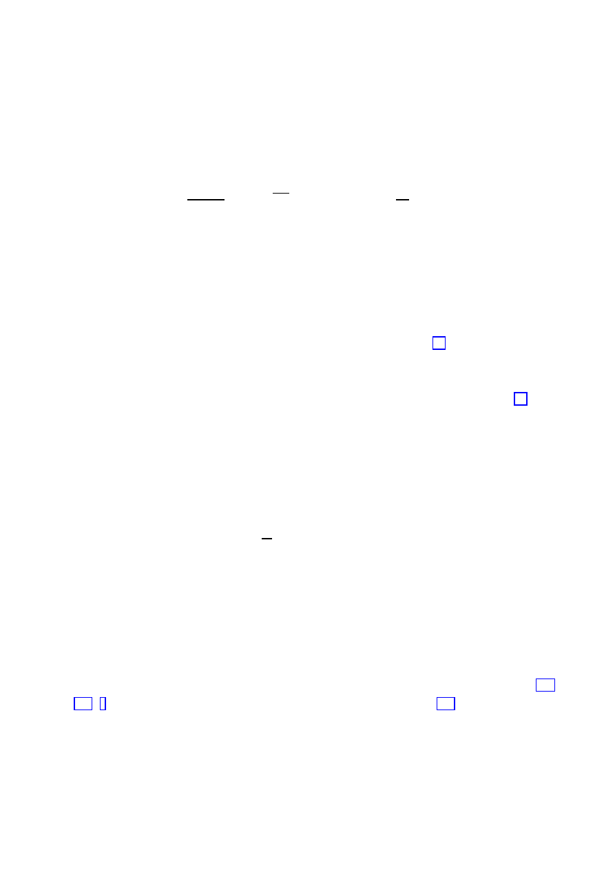
5.1
The beginning of time
Not knowing the correct place to start, a simple guess might be the (bosonic, NS-NS part of
the) low-energy effective action in D dimensions,
S =
−
1
16πG
D
Z
d
D
x
√
−ge
−φ
R + ∂
µ
φ∂
µ
φ
−
1
12
H
µνρ
H
µνρ
,
(65)
where R is the Ricci scalar, φ is the dilaton, and H
µνρ
= ∂
[µ
B
νρ]
is the field strength tensor
for the two-form gauge field B
νρ
(which is typically set to zero in papers about cosmology).
The existence of the dilaton implies that the theory of gravity described by this action
is a scalar-tensor model (reminiscent of Brans-Dicke theory), not pure general relativity.
Of course there are good experimental limits on scalar components to the gravitational
interaction, but they are only sensitive to low-mass scalars (i.e., long-range forces), so that
the dilaton could escape detection if we added a potential V (φ) to (65) which led to a mass
m
φ
> 10
−4
eV
∼ (10
−1
cm)
−1
. As we’ve discussed, it is natural to hope that supersymmetry
breaking induces a mass m
φ
∼ 10
3
GeV, so we would seem quite safe.
So we really should include a potential for φ (not to mention one for B
νρ
) in (65), but
let’s neglect it for now and move boldly forward. With this action, cosmological solutions of
the form
ds
2
=
−dt
2
+
D
−1
X
i=1
a
2
i
(t)dx
2
i
(66)
(homogeneous but not necessarily isotropic) have a “scale-factor duality” symmetry; for any
solution
{a
i
(t), φ(t)
}, there is also a solution with
a
0
i
=
1
a
i
,
φ
0
= φ
− 2
X
i
ln a
i
.
(67)
Thus, expanding solutions are dual to contracting solutions. (In fact this is just T -duality,
and is a subgroup of a larger O(D
− 1, D − 1) symmetry.) What is more, solutions with
decreasing curvature are mapped to those with increasing curvature.
This feature of the low-energy string action has led to the development of the “Pre-Big-
Bang Scenario”, in which the universe starts out as flat empty space, begins to contract
(with increasing curvature), until reaching a “stringy” state of maximum curvature, and
then expands (as curvature decreases) and commences standard cosmological evolution [125,
126, 6]. (For related considerations outside the Pre-BB picture, see [127].)
There are various questions about the Pre-BB scenario. One is a claim that significant
fine-tuning is required in the initial phase, in the sense that any small amount of curvature
37
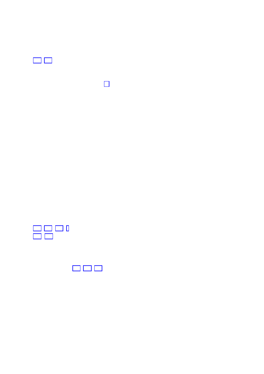
will grow fantastically during the evolutionary process and must be extremely suppressed
[128, 129]. Another is the role of the potential for the dilaton. We cannot set this potential
to zero on the grounds that the relevant temperatures are much higher than the SUSY -
breaking scale T
SUSY
∼ 10
3
GeV; supersymmetry is an example of a symmetry which is not
restored at high temperatures [89]. Indeed, almost any state breaks supersymmetry. In a
thermal background, this breaking is manifested most clearly by the differing occupation
numbers for bosons and fermions. More generally, the SUSY algebra
{Q, ¯
Q
} = H + Z ,
(68)
with Z a central charge, implies that Q
6= 0 whenever H 6= 0, except in BPS states, which
feature a precise cancellation between H and Z. In the real world (in contrast to the
world of hep-th) these are a negligible fraction of all possible states. It is not clear how
SUSY breaking affects the Pre-BB idea.
Perhaps more profoundly, it seems perfectly likely that the appropriate description of
the high-curvature stringy phase will be nothing like a smooth classical spacetime. Evidence
for this comes from matrix theory, not to mention attempts to canonically quantize general
relativity.
There are other, non-stringy, approaches to the very beginning of the universe, and it
would be interesting to know what light can be shed on them by string theory. One is
“quantum cosmology”, which by some definitions is just the study of the wave function
of the universe, although in practice it has the connotation of minisuperspace techniques
(drastically truncating the gravitational degrees of freedom and quantizing what is left)
[130, 121, 131, 7]. There is also the related idea of creation of baby universes from our own
[132, 133]. This is in principle a conceivable scheme, as closed universes have zero total
energy in general relativity. There is also the hope that string theory will offer some unique
resolution to the question of cosmological (and other) singularities; studies to date have had
some interesting results, but we don’t know enough to understand the Big Bang singularity
of the real world [134, 135, 136].
5.2
Extra dimensions and compactification
Of all the features of string theory, the one with the most obvious relevance to cosmology is
the existence of (6? 7?) extra spatial (temporal?) dimensions. The success of our traditional
description of the world as a (3+1)-dimensional spacetime implies that the extra dimensions
must be somehow inaccessible, and the simplest method for hiding them is compactification
38
— the idea that the extra dimensions describe a compact space of sufficiently small size that
they can only be probed by very high energies.
Of course in general relativity (and even in string theory) spacetime is dynamical, and
it would be natural to expect the compact dimensions to evolve. However, the parameters
describing the size and shape of the compact dimensions show up in our low-energy world as
moduli fields whose values affect the Standard Model parameters. As discussed earlier, we
have good limits on any variation of these parameters in spacetime, and typically appeal to
SUSY breaking to fix their expectation values. This raises all sorts of questions. Why are
three dimensions allowed to be large and expanding while the others are small and essentially
frozen? What is the precise origin of the moduli potentials? What was the behavior of the
extra dimensions in the early universe?
For the most part these are baffling questions, although there have been some provocative
suggestions. One is by Brandenberger and Vafa, who attempted to understand the existence
of three macroscopic spatial dimensions in terms of string dynamics [137]. Consider an n-
torus populated by both momentum modes and winding modes of strings. The momentum
and winding modes are dual to each other under T -duality (R
→ 1/R), and have opposite
effects on the dynamics of the torus: the momentum modes tend to make it expand, and
the winding modes to make it contract. (It’s counterintuitive, but true.) We can therefore
have a static universe at the self-dual radius where the two effects are balanced. However,
when wound strings intersect they tend to intercommute and therefore unwind. Through
this process, the balance holding the torus at the self-dual radius can be upset, and the
universe will begin to expand, hopefully evolving into a conventional Friedmann cosmology.
But notice that in a sufficiently large number of spatial dimensions, one-dimensional
strings will generically never intersect. (Just as zero-dimensional points will generically
intersect in one dimension but not in two or more dimensions.) The largest number in which
they tend to intersect is three. So we can imagine a universe that begins as a tiny torus in
thermal equilibrium at the self-dual point, until some winding modes happen to annihilate
in some three-dimensional subspace which then begins to expand, forming our universe. Of
course a scenario such as this loses some of its charm in a theory which has not only strings
but also higher-dimensional branes. (Not to mention that toroidal compactifications are not
pheonomenologically favored.)
An alternate route is to take advantage of the existence of these branes, by imagining
that we are living on one. That is to say, that the reason why the extra dimensions are
invisible to us is not simply because they are so very small that low-energy excitations
39
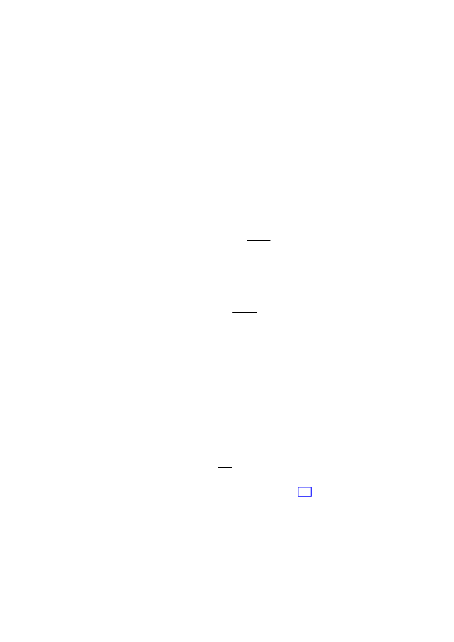
cannot probe them, but because we are confined to a three-dimensional brane embedded in
a higher-dimensional space. We know that we can easily construct field theories confined
to branes, for example a U(N ) gauge theory by stacking N coincident branes; it is not an
incredible stretch to imagine that the entire Standard Model can be constructed in such a
way (although it hasn’t been done yet). Unfortunately, it seems impossible to entirely do
away with the necessity of compactification, since there is one force which we don’t know
how to confine to a brane, namely gravity (although see below).
We therefore imagine a world in which the Standard Model particles are confined to a
three-brane, with gravity propagating in a higher-dimensional “bulk” which includes com-
pactified extra dimensions. In D spacetime dimensions, Newton’s law of gravity can be
written
F
(D)
(r) =
e
G
(D)
m
1
m
2
r
D
−2
,
(69)
where
e
G
(D)
is the D-dimensional Newton’s constant with appropriate factors of 4π absorbed.
If we compactify D
− 4 of the spatial dimensions on a compact manifold of volume V
(D
−4)
,
the effective 4-dimensional Newton’s constant is
e
G
(4)
∼
e
G
(D)
V
(D
−4)
.
(70)
We can rewrite this in terms of what we will define as the Planck scale, M
P
=
e
G
−1/2
(4)
, and
the ”fundamental” scale, M
∗
=
e
G
−1/(D−2)
(D)
, as
M
2
P
∼ M
D
−2
∗
V
(D
−4)
.
(71)
In conventional compactification, M
∗
∼ M
P
and V
(D
−4)
∼ M
−(D−4)
P
, so this relation is
straightforwardly satisfied. But we can also satisfy it by lowering the fundamental scale and
increasing the compactification volume. Imagine that the compactification manifold has n
“large” dimensions of radius R and D
− 4 − n dimensions of radius M
−1
∗
. Then
R
∼
M
P
M
∗
2/n
M
−1
∗
.
(72)
A scenario of this type was proposed by Horava and Witten [138], who suggested that the
gravitational coupling could unify with the gauge couplings of GUT’s by introducing a single
large extra dimension with R
∼ (10
15
GeV)
−1
.
But we can go further. The lowest value we can safely imagine the fundamental scale
having is M
∗
∼ 10
3
GeV; otherwise we would have detected quantum gravity at Fermilab
40
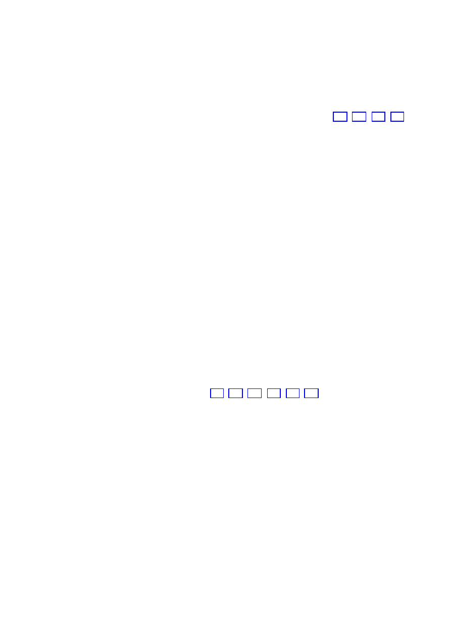
or CERN. This value is essentially the desired low-energy supersymmetry breaking scale
(i.e. just above the electroweak scale), so it is tempting to explain the apparent hierarchy
M
∗
/M
EW
∼ 10
15
by trying to move M
∗
all the way down to 10
3
GeV [139, 140, 141, 142].
(Note that supersymmetry itself can stabilize the hierarchy, but doesn’t actually explain it.)
Then we have
R
∼ 10
30/n
−3
GeV
−1
∼ 10
30/n
−17
cm .
(73)
For n = 1, we have a single extra dimension of radius R
∼ 10
13
cm, about the distance from
the Sun to the Earth. This is clearly ruled out, as such a scenario predicts that gravitational
forces would fall off as r
−3
for distances smaller than 10
13
cm. But for n = 2 we have
R
∼ 10
−2
cm, which is just below the limits on deviations from the inverse square law from
laboratory experiments. Larger n gives smaller values of R; these are not as exciting from
the point of view of having macroscopically big extra dimensions, but may actually be the
most sensible from a physics standpoint.
So we have a picture of the world as a 3-brane with Standard Model particles restricted
to it, and gravity able to propagate into a bulk with extra dimensions which are compactified
but perhaps of macroscopic size, with a fundamental scale M
∗
∼ 10
3
GeV and the observed
Planck scale simply an artifact of the large extra dimensions. (There is still something of
a hierarchy problem, since R must be larger than M
∗
to get the Planck scale right.) Such
scenarios are subject to all sorts of limits from astrophysics and accelerator experiments,
from processes such as gravitons escaping into the bulk. (In these models gravity becomes
strongly coupled near 10
3
GeV.)
There are also going to be cosmological implications, although it is not precisely clear
as yet what these are (see for example [143, 144, 145, 146, 147, 148], not to mention many
papers subsequent to the writing of these notes). Our entire discussion of the thermal history
of the universe for T > 10
3
GeV would obviously need to be discarded. Baryogenesis will
presumably be modified. Inflation is a very interesting question, including the issues of
inflation in the bulk vs. inflation in the boundary. Of course we don’t know what stabilizes
the large extra dimensions, but then again we don’t know much about moduli stabilization
in conventional scenarios. There is also the interesting possibility of a 3-brane parallel to
the one we live on, which only interacts with us gravitationally, and on which the dark
matter resides. There are some cosmological problems, though — most clearly, the issue of
why the bulk is not highly populated by light particles that one might have expected to be
left over from an early high-temperature state; presumably reheating after inflation cannot
be to a very high temperature in these models (although we must at the very least have
41

T
reheat
> 1 MeV to preserve standard nucleosynthesis). Clearly there is a good deal of work
left to do in exploring these scenarios.
After these notes were written, Randall and Sundrum [149] found a loophole in the
conventional wisdom that gravity cannot be confined to a brane. They showed that a single
extra dimension could be infinitely large, but still yield an effective 4-dimensional gravity
theory on the brane, if the bulk geometry were anti-de Sitter rather than flat. The curvature
in the extra dimension can then effectively confine gravity to the vicinity of the brane. In the
subsequent months a great deal of effort has gone into understanding cosmological and other
ramifications of Randall-Sundrum scenarios, which are surely worthy of their own review
article by this point.
5.3
The late universe
The behavior of gravity and particle physics on extremely short length scales and high
energies is largely uncharted territory, and it is clear that string theory, if correct, will play
an important role in understanding this regime. But it is also interesting to contemplate the
possibility of new physics at ultra-large length scales and low energies. You might guess that
experiments in the zero-energy limit are straightforward to perform, but in fact it requires
great effort to isolate yourself from unwanted noise sources in this regime. Cosmology offers
a way to probe physics on the largest observable length scales in the universe, and it is
natural to take advantage.
We spoke in Section 2.5 about the apparent acceleration of the universe, which, if ver-
ified, would be a dramatic indication of new physics at very low energies. Explaining the
observations with a positive vacuum energy ρ
V
= M
4
V
requires
M
V
∼ 10
−3
eV ,
(74)
which is remarkably small in comparison to M
SUSY
∼ 10
3
GeV = 10
12
eV, not to mention
M
P
∼ 10
18
GeV = 10
27
eV. It does, of course, induce the irresistible temptation to write
M
V
∼
M
2
SUSY
M
P
.
(75)
This is a numerological curiosity without a theory that actually predicts it, although it
has the look and feel of similar relations familiar from models in which SUSY breaking is
communicated from one sector to another by gravitational interactions. Another provocative
relation is
M
V
∼ e
−1/2α
M
P
,
(76)
42
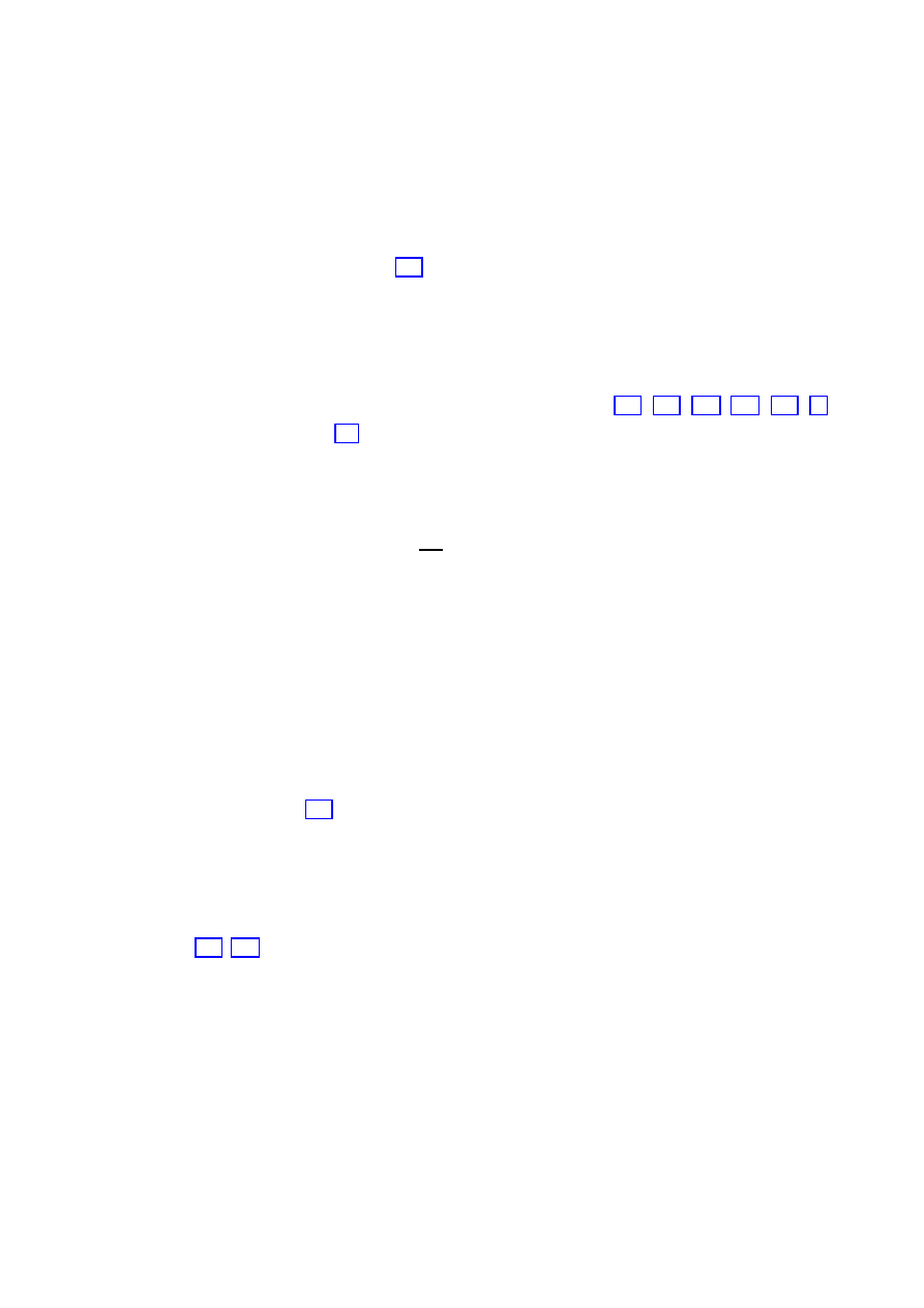
where α is the fine-structure constant. Again, it falls somewhat short of the standards of
a scientific theory, but it does suggest the possibility that the vacuum energy would be
precisely zero if it were not for some small nonperturbative effect. There may even be ways
to get such effects in string theory [150].
More generally, we can classify vacuum energy as coming from one of three categories:
“true vacua”, which are global minima of the energy density; “false vacua”, which are local
but not global minima; and “non-vacua”, which is a way of expressing the idea that we have
not yet reached a local minimum value of the potential energy. For example, we could posit
the existence of a scalar field φ with a very shallow potential [151, 152, 153, 154, 155, 26].
From our analysis in Section 3.4, the field will be overdamped when V
00
< H, and its potential
energy will dominate over its kinetic energy (exactly as in inflation). Such a possibility has
been dubbed “quintessence”. For a quintessence field to explain the accelerating universe,
it must have an effective mass
m
φ
≡
√
V
00
≤ H
0
∼ 10
−33
eV ,
(77)
and a typical range of variation over cosmological timescales
∆φ
∼ M
P
∼ 10
18
GeV .
(78)
From a particle-physics point of view, these parameters seem somewhat contrived, to say
the least. In fact, the same fifth-force experiments and variation-of-constants limits that we
previously invoked to argue against the existence of massless moduli are applicable here,
and point toward the necessity of some additional structure in a quintessence theory in order
to evade these bounds [156]. However, quintessence models have the benefit of involving
dynamical fields rather than a single constant, and it may be possible to take advantage
of these dynamics to ameliorate the “coincidence problem” that Ω
Λ
∼ Ω
M
today (despite
the radically different time dependences of these two quantities). In addition, there may
be more complicated ways to get a time-dependent vacuum energy that are also worth
exploring [157, 158]. The moduli fields of string theory could provide potential candidates for
quintessence, and the acceleration of the universe more generally provides a rare opportunity
for string theory to provide an explanation of an empirical fact.
We could also imagine that string theory may have more profound late-time cosmological
consequences than simply providing a small vacuum energy or ultralight scalar fields. An
interesting move in this direction is to explore the implications of the “holographic prin-
ciple” for cosmology. This principle was inspired by our semiclassical expectation that the
43
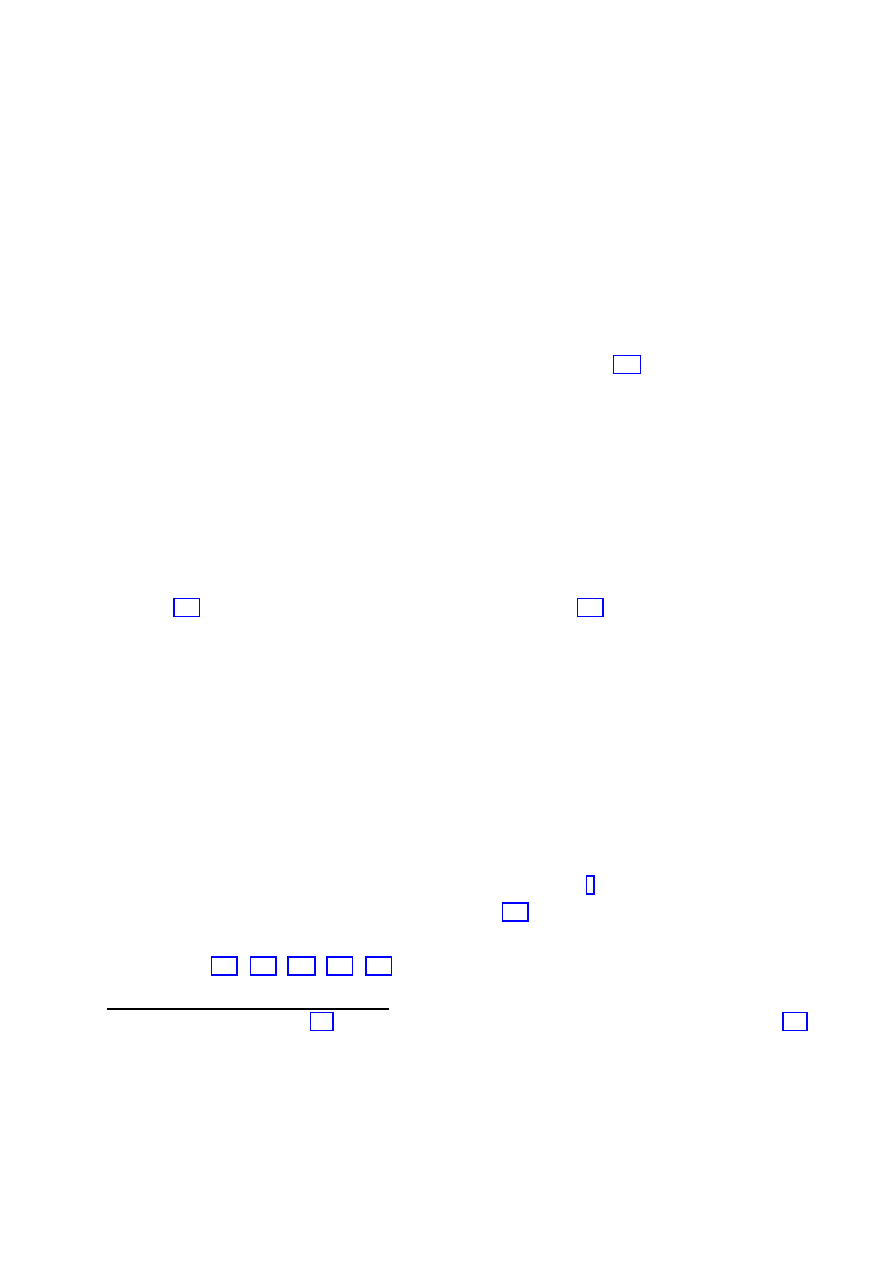
entropy of a black hole, which in traditional statistical mechanics is a measure of the number
of degrees of freedom in the system, scales as the area of the event horizon rather than as
the enclosed volume (as we would expect the degrees of freedom to do in a local quantum
field theory). In its vaguest (and therefore most likely to be correct) form, the holographic
principle proposes that a theory with gravity in n dimensions (or a state in such a theory)
is equivalent in some sense to a theory without gravity in n
− 1 dimensions (or a state in
such a theory). Making this statement more precise is an area of active investigation and
controversy; see Susskind’s lectures for a more complete account [159]. The only context in
which the holographic equivalence has been made at all explicit is in the AdS/CFT corre-
spondence, where the non-gravitational theory can be thought of as living on the spacelike
boundary at conformal infinity of the AdS space on which the gravitational theory lives.
Regrettably, we don’t live in anti-de Sitter space, which corresponds to a RW metric with
a negative cosmological constant and no matter, since our universe seems to feature both
matter and a positive cosmological constant. How might the holographic principle apply
to more general spacetimes, without the properties of conformal infinity unique to AdS, or
for that matter without any special symmetries? A possible answer has been suggested by
Bousso [160], building upon ideas of Fischler and Susskind [161]. The basic idea is to the
area A of the boundary of a spatial volume to the amount of entropy S passing through a
certain null sheet bounded by that surface. (For details of how to construct an appropriate
sheet, see the original references.) Specifically, the conjecture is that
S
≤ A/4G .
(79)
This is more properly an entropy bound, not a claim about holography; however, it seems to
be a short step from limiting entropy (and thus the number of degrees of freedom) to claiming
the existence of an underlying theory dealing directly with those degrees of freedom.
Does this proposal have any consequences for cosmology? It is straightforward to check
that the bound is satisfied by standard cosmological solutions
, and a classical version can
even be proven to hold under certain assumptions [163]. One optimistic hope is that holog-
raphy could be responsible for the small observed value of the cosmological constant (see
for example [164, 165, 166, 167, 168]). Roughly speaking, this hope is based on the idea
that there are far fewer degrees of freedom per unit volume in a holographic theory than
7
It is amusing to note that [161] underestimated the entropy in the current universe, which Penrose [162]
has pointed out is dominated not by photons but by massive black holes at the centers of galaxies, which
have total entropy S
∼ 10
100
. The estimate was therefore off by a factor of 10
14
, although the conclusions
are left unchanged. (This is a common occurrence in cosmology.)
44

local quantum field theory would lead us to expect, and perhaps the unwarranted inclusion
of these degrees of freedom has been leading to an overestimate of the vacuum energy. It
remains to be seen whether a workable implementation of this idea can capture the successes
of conventional cosmology.
6
Conclusions
The last several years have been a very exciting time in string theory, as we have learned
a great deal about non-perturbative aspects of the theory, most impressively the dualities
connecting what were thought to be different theories. They have been equally exciting
in cosmology, as a wealth of new data have greatly increased our knowledge about the
constituents and evolution of the universe. The two subjects still have a long way to go,
however, before their respective domains of established understanding are definitively over-
lapping. One road toward that goal is to work diligently at those aspects of string theory and
cosmology which are best understood, hoping to enlarge these regions until they someday
meet. Another strategy is to leap fearlessly into the murky regions in between, hoping that
our current fumbling attempts will mature into more solid ideas. Both approaches are, of
course, useful and indeed necessary; hopefully these notes will help to empower the next
generation of fearless leapers.
7
Acknowledgments
I’ve benefited from conversations with many colleagues, including Tom Banks, Alan Guth,
Gary Horowitz, Steuard Jensen, Clifford Johnson, Finn Larsen, Donald Marolf, Ue-Li Pen,
Joe Polchinski, Andrew Sornborger, Paul Steinhardt, and Mark Trodden, as well as nu-
merous participants at TASI-99. I would like to thank the organizers (Jeff Harvey, Shamit
Kachru and Eva Silverstein) for arranging a very stimulating school, and the participants
for their enthusiasm and insight. This work was supported in part by the National Science
Foundation under grant PHY/94-07195, the U.S. Department of Energy, and the Alfred P.
Sloan Foundation.
References
45
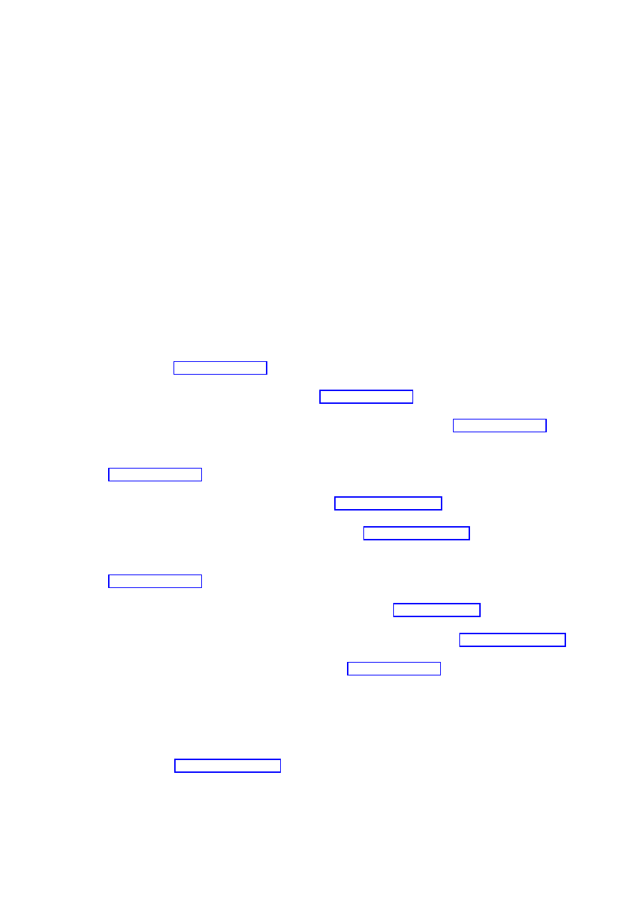
[1] S. Toulmin, in The Early Universe, eds. W.G. Unruh and G.W. Semenoff (Dordrecht:
D. Reidel, 1988).
[2] J. Polchinski, String Theory, two volumes (Cambridge: Cambridge University Press,
1998).
[3] P.J.E. Peebles, Principles of Physical Cosmology (Princeton: Princeton University
Press, 1993).
[4] E.W. Kolb and M.S. Turner, The Early Universe (Redwood City, California: Addison-
Wesley, 1990).
[5] A. Linde, Particle Physics and Inflationary Cosmology (New York: Harwood, 1990).
[6] J. E. Lidsey, D. Wands and E. J. Copeland, “Superstring cosmology,” Phys. Rept. 337,
343 (2000); hep-th/9909061.
[7] T. Banks, “M theory and cosmology,” hep-th/9911067.
[8] G. Veneziano, “String cosmology: The pre-big bang scenario,” hep-th/0002094.
[9] D. A. Easson, ‘The interface of cosmology with string and M(illennium) theory,”
[10] D.H. Lyth, “Introduction to cosmology,” astro-ph/9312022.
[11] E.W. Kolb, “Particle physics and cosmology,” astro-ph/9403007.
[12] R.H.
Brandenberger,
“Particle
physics
aspects
of
modern
cosmology,”
[13] G.F. Ellis and H. van Elst, “Cosmological models,” gr-qc/9812046.
[14] M.S. Turner and J.A. Tyson, Rev. Mod. Phys. 71, S145 (1999); astro-ph/9901113.
[15] G. Lazarides, “Introduction to cosmology,” hep-ph/9904502.
[16] P.J. Peebles, D.N. Schramm, E.L. Turner and R.G. Kron, “The Case for the hot big
bang cosmology,” Nature 352, 769 (1991).
[17] M. Davis, in Critical Dialogues in Cosmology, ed. N. Turok (Singapore, World Scien-
tific, 1997); astro-ph/9610149.
46
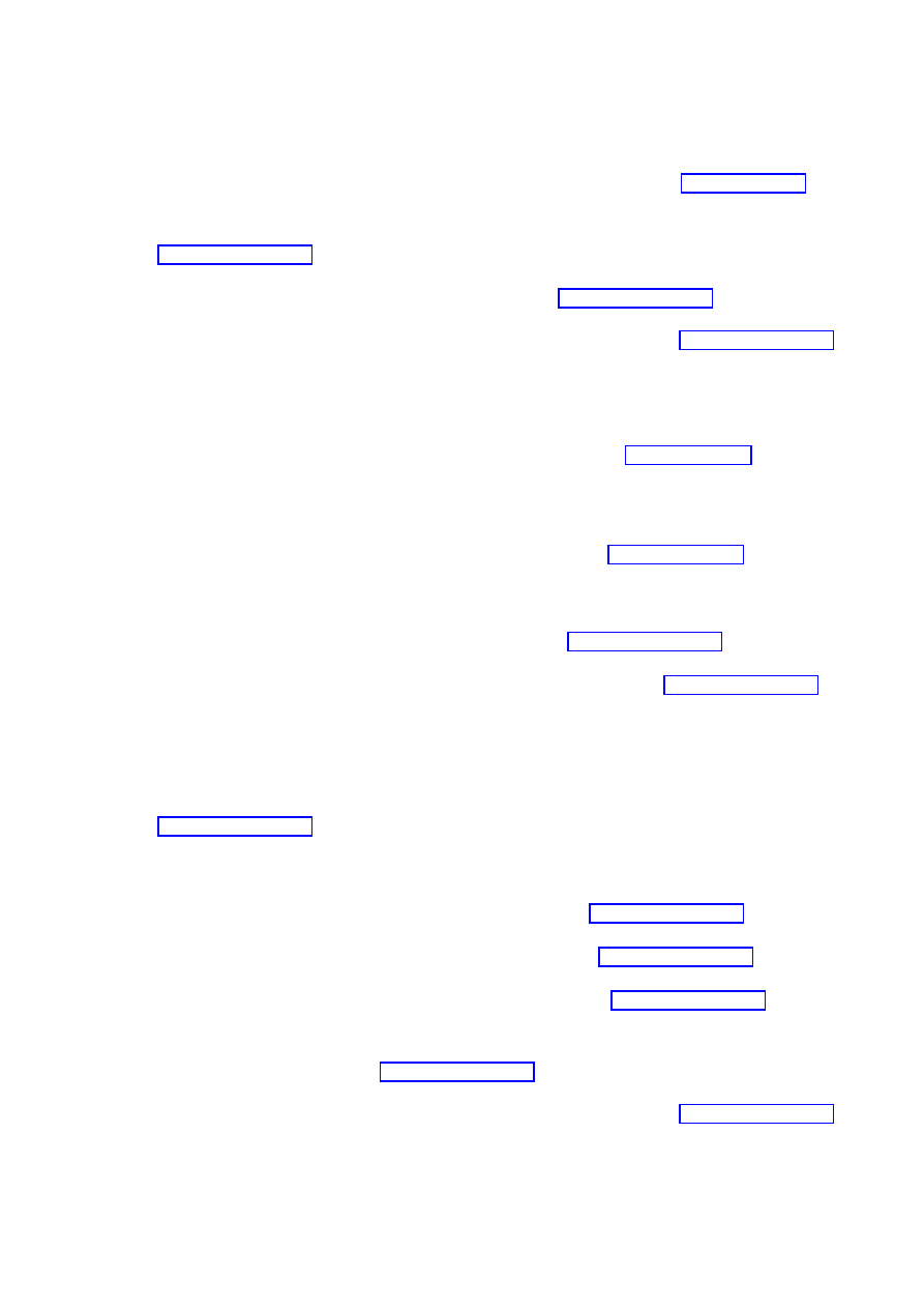
[18] M. Lachi´eze-Rey and J.-P. Luminet, Phys. Rep. 254, 135 (1995); gr-qc/9605010.
[19] N.J. Cornish, D.N. Spergel and G.D. Starkman, Class. Quant. Grav. 15, 2657 (1998);
[20] J.R. Weeks, Class. Quant. Grav. 15, 2599 (1998); astro-ph/9802012.
[21] J. Levin, E. Scannapieco, G. de Gasperis, J. Silk, and J.D. Barrow; astro-ph/9807206.
[22] S.W. Hawking and G.F.R. Ellis, The Large Scale Structure of Space-Time (Cambridge,
Cambridge Univ. Press, 1973).
[23] S.M. Carroll, “Lecture notes on general relativity,” (1997), gr-qc/9712019; also avail-
able at http://pancake.uchicago.edu/~carroll/notes/.
[24] O. Aharony, S. S. Gubser, J. Maldacena, H. Ooguri and Y. Oz, “Large N field theories,
string theory and gravity,” Phys. Rept. 323, 183 (2000) hep-th/9905111.
[25] S. Weinberg, Rev. Mod. Phys. 61, 1 (1989).
[26] S.M. Carroll, Liv. Revs. Gen. Rel., in press (2000); astro-ph/0004075.
[27] W.L. Freedman, “Determination of Cosmological Parameters”, astro-ph/9905222.
[28] M. Persic and P. Salucci, “The baryon content of the universe”, Mon. Not. Roy. Ast.
Soc. 258, 14 (1992).
[29] M. Fukugita, C.J. Hogan and P.J. Peebles, “The Cosmic baryon budget,”
[30] M. Persic, P. Salucci and F. Stel, Mon. Not. Roy. Ast. Soc. 281, 27 (1996).
[31] N.A. Bahcall, “Large scale structure of the universe,” astro-ph/9612046.
[32] J.R. Primack, “Dark matter and structure formation,” astro-ph/9707285.
[33] M.S. Turner, “Dark matter and energy in the universe,” astro-ph/9901109.
[34] A.G. Cohen, A. De Rujula and S.L. Glashow, “A matter-antimatter universe?,” As-
trophys. J. 495, 539 (1998) astro-ph/9707087.
[35] D.N. Schramm and M.S. Turner, Rev. Mod. Phys. 70, 303 (1998); astro-ph/9706069.
47
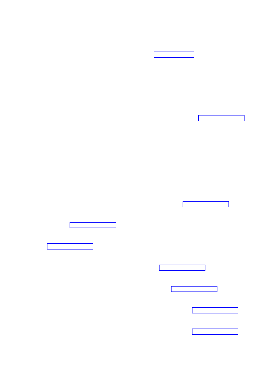
[36] S. Sarkar, Rep. Prog. Phys. 59, 1493 (1996); hep-ph/9602260.
[37] You can calculate the abundances predicted by Big-Bang Nucleosynthesis for your-
self, using a Java applet written by L. Mendoza and C.J. Hogan, available at
http://www.astro.washington.edu/research/bbn/
.
[38] E.G. Zweibel and C. Heiles, Nature 385, 131 (1997).
[39] A.V. Olinto, in Proceedings of the 3rd RESCEU Symposium, University of Tokyo,
Nov. 10-13, 1997, Ed. K. Sato, T. Yanagida, and T. Shiromizu; astro-ph/9807051.
[40] J.H. Krolik, Active Galactic Nuclei (Princeton: Princeton University Press, 1998).
[41] D.O. Richstone, Nature 395, 14 (1998).
[42] Y. Dabrowski, A.C. Fabian, K. Iwasawa, A.N. Lasenby, and C.S. Reynolds, Monthly
Not. Royal Astron. Soc. 288, L11 (1997).
[43] M.T. Ressell and M.S. Turner, Comments Astrophys. 14, 323 (1990).
[44] D.J. Fixsen et al., Astrophys. J. 473, 576 (1996).
[45] W. Hu, N. Sugiyama and J. Silk, Nature 386, 37 (1997); astro-ph/9604166.
[46] M. Kamionkowski and A. Kosowsky, “The cosmic microwave background and particle
physics,” astro-ph/9904108.
[47] R.B. Barreiro,
“The Cosmic Microwave Background:
State of the Art,”
[48] A. D. Miller et al., “A Measurement of the Angular Power Spectrum of the CMB from
l = 100 to 400,” Astrophys. J. 524, L1 (1999); astro-ph/9906421.
[49] A. Melchiorri et al., “A measurement of Omega from the North American test flight
of BOOMERANG,” Astrophys. J. 536, L63 (2000); astro-ph/9911445.
[50] P. de Bernardis et al., “A Flat Universe from High-Resolution Maps of the Cosmic
Microwave Background Radiation,” Nature 404, 955 (2000); astro-ph/0004404.
[51] S. Hanany et al., “MAXIMA-1: A Measurement of the Cosmic Microwave Background
Anisotropy on angular scales of 10 arcminutes to 5 degrees,” astro-ph/0005123.
48
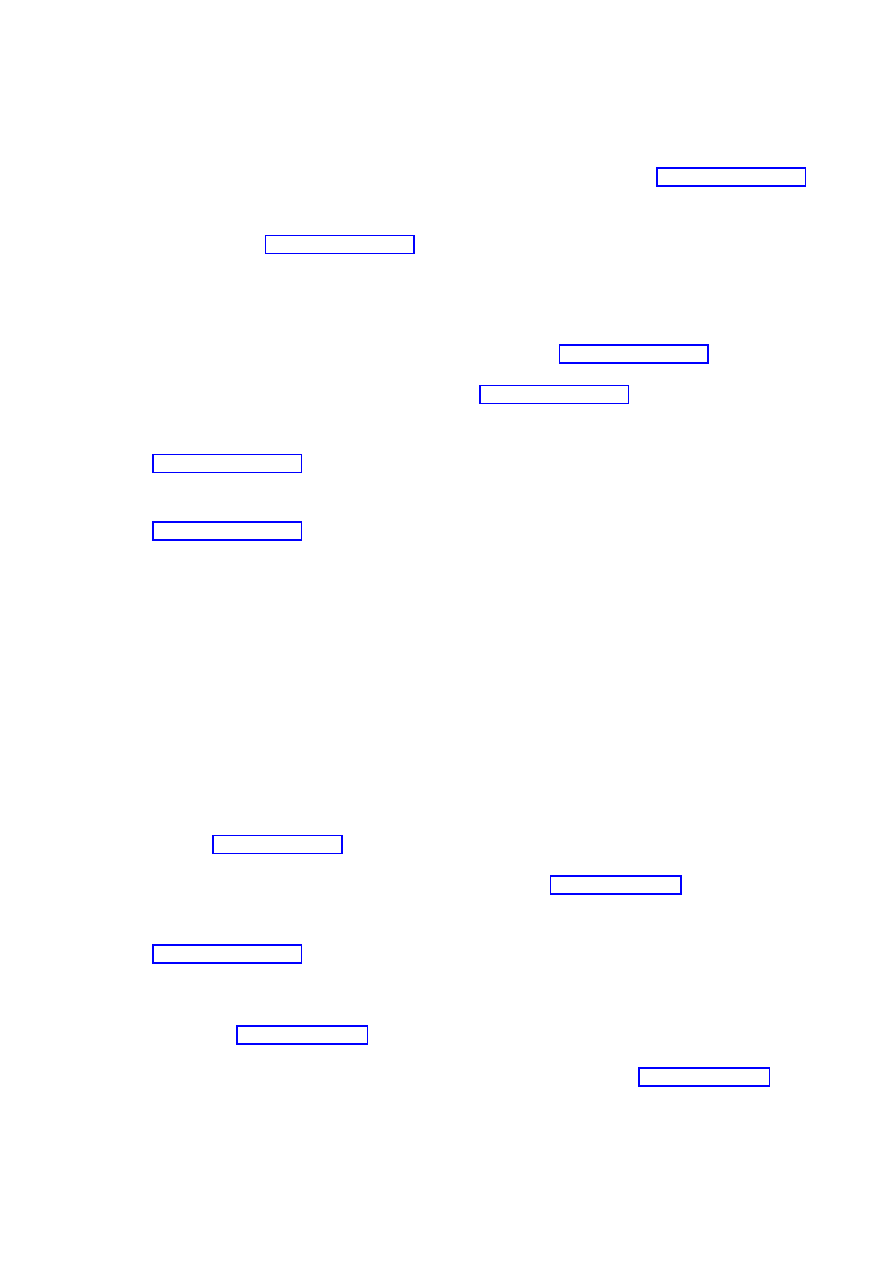
[52] W. Hu and M. White, “Measuring the curvature of the universe,” astro-ph/9606140.
[53] S. Weinberg, “Curvature Dependence of Peaks in the Cosmic Microwave Background
Distribution,” astro-ph/0006276.
[54] U. Seljak and M. Zaldarriaga, Astrophys. J. 469, 437 (1996); for the CMBFAST code,
see http://www.sns.ias.edu/~matiasz/CMBFAST/cmbfast.html.
[55] A.G. Riess et al., Astronomical J. 116, 1009 (1998); astro-ph/9805201.
[56] S. Perlmutter et al., Astrophys. J. (1999); astro-ph/9812133.
[57] V. Sahni and A. Starobinsky, “The case for a positive cosmological lambda-term,”
[58] M.S.
Turner,
“Why
cosmologists
believe
the
universe
is
accelerating,”
[59] S.M. Carroll, W.H. Press, and E.L. Turner, Annu. Rev. Astron. Astrophys. 30, 499
(1992).
[60] C.B. Collins and S.W. Hawking, Astrophys. J. 180, 317 (1973).
[61] A. Vilenkin and E.P.S. Shellard, Cosmic Strings and Other Topological Defects (Cam-
bridge: Cambridge Univ. Press, 1994).
[62] N. Steenrod, The Topology of Fibre Bundles (Princeton: Princeton University Press,
1970).
[63] J. A. Bryan, S. M. Carroll and T. Pyne, “A Texture bestiary,” Phys. Rev. D50, 2806
(1994); hep-ph/9312254.
[64] Y. Fukuda et al., Phys. Rev. Lett. 81, 1562 (1998); hep-ex/9807003.
[65] J.R. Primack and M.A. Gross, “Cold + hot dark matter after Super-Kamiokande,”
[66] A.D. Dolgov, “NonGUT baryogenesis,” Phys. Rept. 222, 309 (1992).
[67] A. Riotto, hep-ph/9807454.
[68] A. Riotto and M. Trodden, “Recent progress in baryogenesis,” hep-ph/9901362.
49
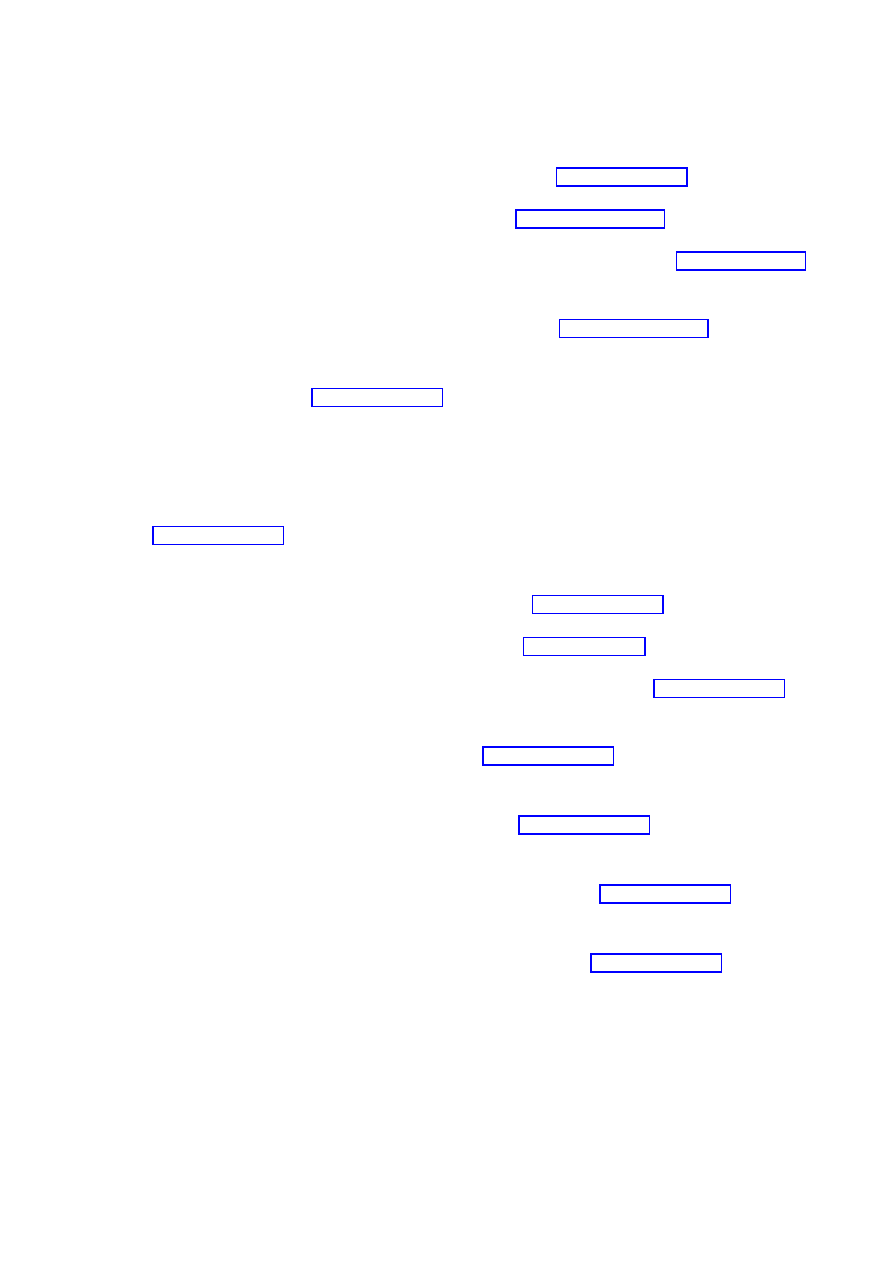
[69] E.W. Kolb, “Particle physics in the early universe,” hep-ph/9810362.
[70] J. Ellis, “Particle candidates for dark matter,” astro-ph/9812211.
[71] G. Baym, D. Bodeker and L. McLerran, Phys. Rev. D53, 662 (1996) hep-ph/9507429.
[72] M. Joyce and M. Shaposhnikov, “Primordial magnetic fields, right electrons, and the
Abelian anomaly,” Phys. Rev. Lett. 79, 1193 (1997) astro-ph/9703005.
[73] O. Tornkvist, “On the electroweak origin of cosmological magnetic fields,” Phys. Rev.
D58, 043501 (1998) hep-ph/9707513.
[74] I. Affleck and M. Dine, “A New Mechanism For Baryogenesis,” Nucl. Phys. B249, 361
(1985).
[75] A.V. Smilga, “Physics of hot and dense QCD,” Nucl. Phys. A654, 136 (1999)
[76] B.A. Campbell and K.A. Olive, “Nucleosynthesis and the time dependence of funda-
mental couplings,” Phys. Lett. B345, 429 (1995) hep-ph/9411272.
[77] J.D. Barrow, “Varying G and other constants,” gr-qc/9711084.
[78] T. Moroi, “Effects of the gravitino on the inflationary universe,” hep-ph/9503210.
[79] R. Kallosh, L. Kofman, A. Linde and A. Van Proeyen, “Gravitino production after
inflation,” Phys. Rev. D61, 103503 (2000) hep-th/9907124.
[80] G. F. Giudice, I. Tkachev and A. Riotto, “Non-thermal production of dangerous relics
in the early universe,” JHEP 9908, 009 (1999) hep-ph/9907510.
[81] G. F. Giudice, A. Riotto and I. Tkachev, “Thermal and non-thermal production of
gravitinos in the early universe,” JHEP 9911, 036 (1999) hep-ph/9911302.
[82] A. Buonanno, M. Lemoine and K. A. Olive, “Reheating and dangerous relics in pre-big
bang string cosmology,” Phys. Rev. D62, 083513 (2000) hep-th/0006054.
[83] K. Maeda, “On Time Variation Of Fundamental Constants In Superstring Theories,”
Mod. Phys. Lett. A3, 243 (1988).
50
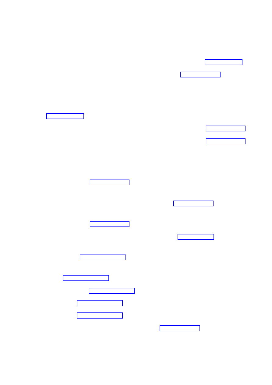
[84] T. Damour, in Les Houches Summer School on Gravitation and Quantizations, eds. J.
Zinn-Justin and B. Julia, Les Houches, France, 5 Jul - 1 Aug 1992, gr-qc/9606079.
[85] T. Damour and F. Dyson, Nucl. Phys. B480, 37 (1996), hep-ph/9606486.
[86] G.D. Coughlan, W. Fischler, E.W. Kolb, S. Raby and G.G. Ross, “Cosmological Prob-
lems For The Polonyi Potential,” Phys. Lett. B131, 59 (1983).
[87] B. de Carlos, J.A. Casas, F. Quevedo and E. Roulet, Phys. Lett. B318, 447 (1993)
[88] T. Banks, D.B. Kaplan and A.E. Nelson, Phys. Rev. D49, 779 (1994) hep-ph/9308292.
[89] M. Dine, L. Randall and S. Thomas, Phys. Rev. Lett. 75, 398 (1995); hep-ph/9503303.
[90] M. Dine and N. Seiberg, “Is The Superstring Weakly Coupled?,” Phys. Lett. B162,
299 (1985).
[91] R. Brustein and P. J. Steinhardt, “Challenges for superstring cosmology,” Phys. Lett.
B302, 196 (1993) hep-th/9212049.
[92] G. Huey, P. J. Steinhardt, B. A. Ovrut and D. Waldram, “A cosmological mechanism
for stabilizing moduli,” Phys. Lett. B476, 379 (2000) hep-th/0001112.
[93] M. Dine, “Towards a solution of the moduli problems of string cosmology,” Phys. Lett.
B482, 213 (2000) hep-th/0002047.
[94] M. Dine, “TASI lectures on M theory phenomenology,” hep-th/0003175.
[95] A.R. Liddle and D.H. Lyth, “The Cold dark matter density perturbation,” Phys. Rept.
231, 1 (1993) astro-ph/9303019.
[96] S. Dodelson, E.I. Gates and M.S. Turner, “Cold dark matter models,” Science 274, 69
(1996) astro-ph/9603081.
[97] M. Sakellariadou, astro-ph/9911497.
[98] A. Albrecht, astro-ph/0009129.
[99] L. Pogosian, astro-ph/0009307.
[100] A. Linde, “Lectures on inflationary cosmology,” hep-th/9410082.
51
[101] E.W. Kolb, “Inflation in the postmodern era,” astro-ph/9612138.
[102] M.S. Turner, “Ten things everyone should know about inflation,” astro-ph/9704062.
[103] R.H. Brandenberger, “Inflation and the Theory of Cosmological Perturbations”,
[104] W.G. Unruh, in Critical Dialogues in Cosmology, ed. N. Turok (Singapore, World
Scientific, 1997).
[105] A.R. Liddle, “An Introduction to cosmological inflation,” astro-ph/9901124.
[106] A. H. Guth, “Inflation and eternal inflation,” Phys. Rept. 333-334, 555 (2000)
[107] L. Kofman, A. Linde and A. Starobinsky, “Towards the Theory of Reheating After
Inflation”, Phys. Rev. D 56, 3258 (1997); hep-ph/9704452.
[108] D. Boyanovsky, D. Cormier, H. J. de Vega, R. Holman, and S.P. Kumar, “Out of
Equilibrium Fields in Inflationary Dynamics. Density Fluctuations”, hep-ph/9801453.
[109] L. Randall, “Supersymmetry and inflation,” hep-ph/9711471.
[110] D.H. Lyth and A. Riotto, “Particle physics models of inflation and the cosmological
density perturbation,” hep-ph/9807278.
[111] A. Linde, “Hybrid inflation,” Phys. Rev. D49, 748 (1994) astro-ph/9307002.
[112] E.J. Copeland, A.R. Liddle, D.H. Lyth, E.D. Stewart and D. Wands, “False vacuum
inflation with Einstein gravity,” Phys. Rev. D49, 6410 (1994) astro-ph/9401011.
[113] D. Wands, “Extended gravity theories and the Einstein-Hilbert action,” Class. Quant.
Grav. 11, 269 (1994); gr-qc/9307034.
[114] T. Banks, M. Berkooz, S.H. Shenker, G. Moore and P.J. Steinhardt, “Modular cos-
mology,” Phys. Rev. D52, 3548 (1995); hep-th/9503114.
[115] T. Banks, “Remarks on M theoretic cosmology,” hep-th/9906126.
[116] V.F. Mukhanov, H.A. Feldman and R.H. Brandenberger, Phys. Rept. 215, 203 (1992);
52
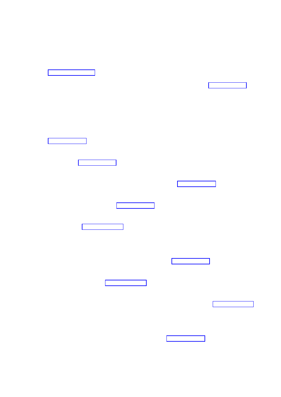
[117] J.E. Lidsey, A.R. Liddle, E.W. Kolb, E.J. Copeland, T. Barreiro and M. Abney, “Re-
constructing the inflation potential : An overview,” Rev. Mod. Phys. 69, 373 (1997)
[118] T. Vachaspati and M. Trodden, “Causality and cosmic inflation,” gr-qc/9811037.
[119] A. Vilenkin, “The Birth Of Inflationary Universes,” Phys. Rev. D27, 2848 (1983).
[120] A.D. Linde, “Eternally Existing Selfreproducing Chaotic Inflationary Universe,” Phys.
Lett. B175, 395 (1986).
[121] A. Linde, “Quantum cosmology and the structure of inflationary universe,”
[122] A. Vilenkin, “Making predictions in eternally inflating universe,” Phys. Rev. D52,
3365 (1995) gr-qc/9505031.
[123] A. Linde, D. Linde and A. Mezhlumian, “From the Big Bang theory to the theory of
a stationary universe,” Phys. Rev. D49, 1783 (1994) gr-qc/9306035.
[124] A. Borde and A. Vilenkin, “Singularities in inflationary cosmology: A Review,” Int. J.
Mod. Phys. D5, 813 (1996) gr-qc/9612036.
[125] M. Gasperini and G. Veneziano, “Pre - big bang in string cosmology,” Astropart. Phys.
1, 317 (1993) hep-th/9211021.
[126] For
a
web
page
devoted
to
the
pre-Big
Bang
scenario,
see
http://www.to.infn.it/~gasperin/
.
[127] J.D. Barrow and K.E. Kunze, “String cosmology,” gr-qc/9807040.
[128] M.S. Turner and E.J. Weinberg, “Pre big bang inflation requires fine tuning,” Phys.
Rev. D56, 4604 (1997) hep-th/9705035.
[129] N. Kaloper, A. Linde and R. Bousso, “Pre-big bang requires the universe to be exponen-
tially large from the very beginning,” Phys. Rev. D59, 043508 (1999) hep-th/9801073.
[130] J.B. Hartle and S.W. Hawking, “Wave Function Of The Universe,” Phys. Rev. D28,
2960 (1983).
[131] A. Vilenkin, “The Quantum cosmology debate,” gr-qc/9812027.
53
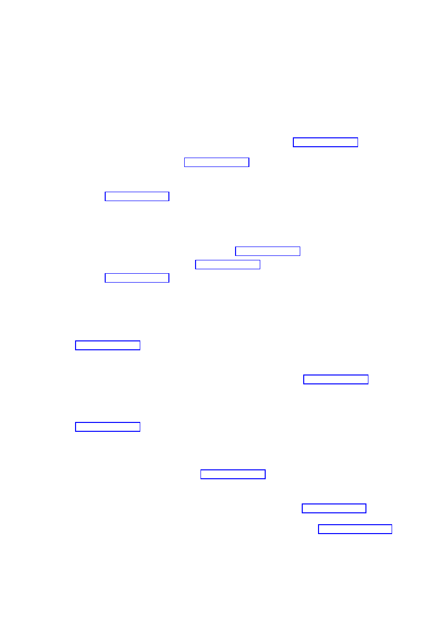
[132] E. Farhi, A.H. Guth and J. Guven, “Is It Possible To Create A Universe In The
Laboratory By Quantum Tunneling?,” Nucl. Phys. B339, 417 (1990).
[133] W. Fischler, D. Morgan and J. Polchinski, Phys. Rev. D42, 4042 (1990).
[134] F. Larsen and F. Wilczek, Phys. Rev. D55, 4591 (1997); hep-th/9610252.
[135] M. Maggiore and A. Riotto, hep-th/9811089.
[136] T. Banks, W. Fischler and L. Motl, “Dualities versus singularities,” JHEP 01, 019
(1999); hep-th/9811194.
[137] R. Brandenberger and C. Vafa, “Superstrings In The Early Universe,” Nucl. Phys.
B316, 391 (1989).
[138] E. Witten, Nucl. Phys. B471, 135 (1996), hep-th/9602070; P. Horava and E. Witten,
Nucl. Phys. B475, 94 (1996), hep-th/9603142; P. Horava, Phys. Rev. D 54, 7561
(1996), hep-th/9608019.
[139] I. Antoniadis, “A Possible New Dimension At A Few Tev,” Phys. Lett. B246, 377
(1990).
[140] J. D. Lykken, “Weak Scale Superstrings,”
Phys. Rev. D54, 3693 (1996);
[141] N. Arkani-Hamed, S. Dimopoulos and G. Dvali, “The hierarchy problem and new
dimensions at a millimeter,” Phys. Lett. B429, 263 (1998); hep-ph/9803315.
[142] I. Antoniadis, N. Arkani-Hamed, S. Dimopoulos and G. Dvali, “New dimensions at
a millimeter to a Fermi and superstrings at a TeV,” Phys. Lett. B436, 257 (1998);
[143] N. Arkani-Hamed, S. Dimopoulos and G. Dvali, “Phenomenology, astrophysics and
cosmology of theories with submillimeter dimensions and TeV scale quantum gravity,”
Phys. Rev. D59, 086004 (1999); hep-ph/9807344.
[144] N. Arkani-Hamed, S. Dimopoulos, N. Kaloper and J. March-Russell, “Early inflation
and cosmology in theories with submillimeter dimensions,” hep-ph/9903239.
[145] J.D. Lykken, “New and improved superstring phenomenology,” astro-ph/9903026.
54
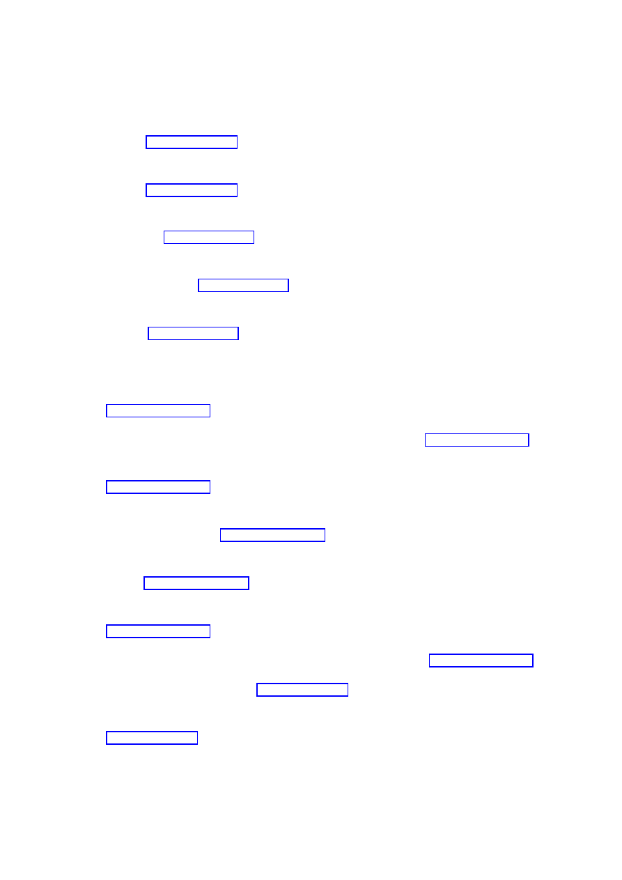
[146] T. Banks, M. Dine and A. Nelson, “Constraints on theories with large extra dimen-
sions,” hep-th/9903019.
[147] L.J. Hall and D. Smith, “Cosmological constraints on theories with large extra dimen-
sions,” hep-ph/9904267.
[148] P. Binetruy, C. Deffayet and D. Langlois, “Nonconventional cosmology from a brane
universe,” hep-th/9905012.
[149] L. Randall and R. Sundrum, “An alternative to compactification,” Phys. Rev. Lett.
83, 4690 (1999); hep-th/9906064.
[150] J.A. Harvey, “String duality and nonsupersymmetric strings,” Phys. Rev. D59, 026002
(1999); hep-th/9807213.
[151] B. Ratra and P.J.E. Peebles, Phys. Rev. D 37, 3406 (1988).
[152] J. Frieman, C. Hill, A. Stebbins, and I. Waga, Phys. Rev. Lett. 75, 2077 (1995),
[153] M.S. Turner and M. White, Phys. Rev. D 56, 4439 (1997), astro-ph/9701138.
[154] R.R. Caldwell, R. Dave and P.J. Steinhardt, Phys. Rev. Lett. 80, 1582 (1998),
[155] P.J. Steinhardt, L. Wang and I. Zlatev, “Cosmological tracking solutions,” Phys. Rev.
D59, 123504 (1999); astro-ph/9812313.
[156] S.M. Carroll, “Quintessence and the rest of the world,” Phys. Rev. Lett. 81, 3067
(1998) astro-ph/9806099.
[157] G.W. Anderson and S.M. Carroll, “Dark matter with time-dependent mass”,
[158] M. Bucher and D.N. Spergel, “Is the dark matter a solid?,” astro-ph/9812022.
[159] D. Bigatti and L. Susskind, hep-th/0002044.
[160] R. Bousso, “Holography in general space-times,” JHEP 9906, 028 (1999);
55
[161] W. Fischler and L. Susskind, hep-th/9806039.
[162] R. Penrose, in Fourteenth Texas Symposium on Relativistic Astrophysics, ed. E.J.
Fenyves (New York Acad. Sci., 1989).
[163] E. E. Flanagan, D. Marolf and R. M. Wald, “Proof of Classical Versions of the Bousso
Entropy Bound and of the Generalized Second Law,” Phys. Rev. D62, 084035 (2000)
[164] T. Banks, “SUSY breaking, cosmology, vacuum selection and the cosmological con-
stant in string theory,” hep-th/9601151.
[165] A.G. Cohen, D.B. Kaplan and A.E. Nelson, “Effective field theory, black holes, and
the cosmological constant,” hep-th/9803132.
[166] P. Horava and D. Minic, “Probable values of the cosmological constant in a holographic
theory,” Phys. Rev. Lett. 85, 1610 (2000) hep-th/0001145.
[167] T. Banks, “Cosmological breaking of supersymmetry or little Lambda goes back to the
future II,” hep-th/0007146.
[168] S. Thomas, “Holographic vacuum energy,” hep-th/0010145.
56
Wyszukiwarka
Podobne podstrony:
Barber Adagio For Strings (Score)
Norbury General relativity and cosmology for undergraduates (Wisconsin lecture notes, 1997)(116s)
Tiësto Adagio for Strings (DjFlo) piano version
Adagio for Strings & Organ Albinoni
adagio for strings
The Beatles For String Quartet Yesterday Sheet Music
Mieczysław Karłowicz Serenade for Strings, Op 2 (1897) YouTube
Samuel Barber Adagio For Strings Op 11 (piano)
Albinoni Concerto for Strings Score
Arrangement Adagio for Strings
Barber, Samuel Adagio For Strings op 11
barber Adagio for strings
Barber Adagio For Strings, Op 11 (full score)
[Clarinet Institute] Rossini, Gioacchino Variations for Clarinet and Strings
bach wilhelmj air for the g string
An Empirical Comparison of C C Java Perl Python Rexx and Tcl for a Search String Processing Pro
więcej podobnych podstron