Microsoft Word - Marie Colombie exjobb 2007.9.doc

Hydrological study for a mini-hydropower plant in the Pyrenees

Master’s thesis in the International Master’s Programme Applied Environmental
Measurement Techniques

COLOMBIE MARIE

Department of Civil and Environmental Engineering
Division of Water Environment Technology

CHALMERS UNIVERSITY OF TECHNOLOGY
Göteborg, Sweden, 2007
Master’s Thesis 2007:9

MASTER’S THESIS 2007:9

Hydrological study for a mini-hydropower plant in

the Pyrenees

COLOMBIE MARIE

Department of Civil and Environmental Engineering

Division of Water Environment Technology

CHALMERS UNIVERSITY OF TECHNOLOGY

Göteborg, Sweden, 2007

Hydrological study for a mini-hydropower plant in the Pyrenees

COLOMBIE Marie

Master’s Thesis 2007:9

Department of Civil and Environmental Engineering

Division of Water Environment Technology

CHALMERS UNIVERSITY OF TECHNOLOGY

SE-412 96 Göteborg

Sweden

Telephone: +46 (0)31-772 1000

Cover:

Picture of Le Siouré and the Siouré’s watershed (23/10/2006)....

Hydrological study for a mini-hydropower plant in the Pyrenees

COLOMBIE Marie

Department of Civil and Environmental Engineering

Division of Water Environment Technology

CHALMERS UNIVERSITY OF TECHNOLOGY

ABSTRACT

Energy refers to the most important issue in the world. The demand is always higher whereas
the production is a source of pollution. Thus Kyoto protocol encourages renewable energies
such as hydraulic power. The construction of a mini-hydropower plant requires a detailed
feasibility study to plan the harnessing strategy and the profitability.

The chosen site is located in the Pyrenees and consists in two small streams. The flow is low,
however the difference in height is very interesting, around 450m. The goal of the following
study is to determine the hydrograph and the flow frequency diagram for two different scenarios
of construction. It also presents the software HEC-HMS, which is capable of simulating the
precipitation-runoff processes of watershed systems. It is often used by hydrologists; so it is a
good way to acquire a certain command of the software, very useful for the future.

A first way of calculation is the statistics. By some correlations with neighbour rivers,
hydrographs can be determined. The second method consists in simulations with HEC-HMS by
defining parameters and specific criteria such as evapotranspiration and snowmelt in order to
adapt the build model with this specific area. The comparison of the two methods allows to
confirm the results and to criticise the chosen model and its calibration in HEC-HMS.

The results are globally satisfying; however a lack of data is always met. Even if the report
presents a consequent bibliography work, extrapolations and judicious tries, more data would
permit a more precise graph. For example, temperature values and details on geographical
characteristics are required to continue. Moreover, before the construction work, flow gages
have to be placed on the streams, at least during one year to complete this analysis.

Key word

: Hydraulic power plant, precipitation-runoff processes, statistical hydrology.

ACKNOWLEDGEMENT

I express my first thanks to Jacques BERTRAND, representative to ORUS, village in south of
France, who trust my team to do the entire study with independence. It is rare to accord so
much confidence in students. I hope we answer well to all his expectations.

I want to thank all the professors who help me during the entire study by giving relevant advice
and by answering each time very rapidly to my questions. I think particularly to Marie-Madeleine
MAUBOURGUET and Denis DARTUS, researchers in the Fluid Mechanics Institute in Toulouse
(IMFT).

The professional contacts were also very interesting. I want especially to thank Philippe
DUCHEVET, engineer at ESTEBE, and Denis MOSNIER, hydrologist at EDF (electricity
supplier in France). They were also very present and allow me to stand back and to have a
better judgment on each step of the study.

I thank also Lars Bergdahl, my supervisor and examiner in CHALMERS, and Sébastien Rauch
for their help despite the distance which separates us.

Finally I thank my colleagues for their serious and the energy they put in the project. Even if
each task was very different, we always keep contact to explain each step of the different
studies. It was very interesting to learn about different fields.

Marie Colombie exjobb 2007.9

Page 7/31

TABLE OF CONTENTS

Introduction ____________________________________________________________________ 9

Aims and goals _________________________________________________________________ 10

Context _______________________________________________________________________ 11

3.1

Who?_____________________________________________________________________ 11

3.2

The team__________________________________________________________________ 11

3.3

General site view ___________________________________________________________ 11

3.4

Detailed studied area________________________________________________________ 12

3.5

First estimations ___________________________________________________________ 13

GIS watershed delineation ________________________________________________________ 14

4.1

The definition of a watershed _________________________________________________ 14

4.2

GIS: the geographical information system ______________________________________ 14

Method 1: A hydrograph based on Statistic analysis ___________________________________ 16

5.1

Collection of the most relevant data ___________________________________________ 16

5.2

Frequency flow diagram _____________________________________________________ 16

5.3

The Compensation flow _____________________________________________________ 19

5.4

Hydrograph _______________________________________________________________ 21

Method 2: HEC-HMS, precipitation-runoff model_____________________________________ 22

6.1

Data collection _____________________________________________________________ 22

6.2

General model in the software ________________________________________________ 22

6.3

Limits of the simple model ___________________________________________________ 24

6.4

Evapotranspiration _________________________________________________________ 25

6.5

Snowmelt _________________________________________________________________ 25

Final results ___________________________________________________________________ 29

Conclusion ____________________________________________________________________ 31

References_____________________________________________________________________ 32

Marie Colombie exjobb 2007.9

Page 8/31

TABLE OF ILLUSTRATIONS

Figure 1. Location of the area in the ARIEGE, part of the Pyrenees (Hola Andorra, 2006) ......... 9

Figure 2. Locations of the different investigated points near Vicdessos. (IGN, 2006)................ 11

Figure 3. The investigated area in detail. (Sandre, 2006) .......................................................... 12

Figure 4. Watershed description. (Wikipedia, 2006) .................................................................. 14

Figure 5. Watersheds bounderies drawn by ArcGis simulation.................................................. 15

Figure 6. Linear correlation between L'Artigue and Le Suc-Sentenac. ...................................... 17

Figure 7. Frequency flow diagram representing the association of the two rivers. .................... 18

Figure 8. Flow frequency diagram for Le Siouré. ....................................................................... 19

Figure 9. Flow average variations made over forty years. ......................................................... 21

Figure 10. Infiltration rates influence on the hydrograph. ........................................................... 23

Figure 11. Comparison of the statistical model and the HEC-HMS simulation. ......................... 25

Figure 12. Different snowmelt models based on Martinac 's theory........................................... 27

Figure 13. Parameterisation of the five alti-zones. ..................................................................... 27

Figure 14. Snowmelt coefficient influence on the hydrograph.................................................... 28

Figure 15. Final comparison of HEC-HMS and statistic for Siouré's hydrograph....................... 29

Figure 16. Influence of temperature data changes on the peaks in the hydrograph. ................. 30

Table 1. Surface values for the different watersheds. ................................................................ 14

Table 2. Monthly averages calculated by the Myer formula ....................................................... 18

Table 3. Baseflow choices for each month in l/s. ....................................................................... 24

Table 4. Total evapotranspiration and rainfall values for 2005 (Météofrance, 2006). ................ 25

Table 5. Chosen criteria for the snowmelt model. ...................................................................... 26

Table 6. Entered data for temperature variations during an anomaly. ....................................... 30

TABLE OF APPENDIX

Appendix 1. Example of an interface in HEC-HMS.

Marie Colombie exjobb 2007.9

Page 9/31

1 INTRODUCTION

The Kyoto protocol encourages renewable energies to avoid the emission of carbon dioxide to
the atmosphere. This issue is more and more present in the media and political programs.
Actions have to be taken in order to improve the situation. Apparently, a small-scale hydropower
is one of the most cost-effective and reliable energy technologies which is considered for
providing clean electricity generation. This is why the French government provides financial aids
to inhabitants or organizations who wish to install this kind of structures.

The French Pyrenees have a very attractive topography and morphology for mini-hydro
projects. These mountains are home to several hundreds of rivers, abrupt slopes and snow to
feed streams during the melt.

Before planning this costly construction, specialists are in charge of a serious and meticulous
feasibility study. Here, the project deals with the feasibility of a mini-hydropower plant in the
ARIEGE, a region in the Pyrenees showed in Figure 1. Some representatives of the towns
surrounding are very interested in harnessing some of the streams which are running through
the area. This report will particularly deal with the study of the hydrologic characteristics of the
location to answer their expectations.

Figure 1. Location of the area in the ARIEGE, part of the Pyrenees (Hola Andorra, 2006)

Marie Colombie exjobb 2007.9

Page 10/31

2 AIMS AND GOALS

The main goal is to draw the annual mean water resource in order to determine the useable
flow which could go through the turbine. To do that, two different methods are used:

Statistical analysis

using data of neighbour rivers allows determining the water

resources of the investigated area by correlations.

Numerical analysis

allows simulating the flows helped by rainfall patterns,

topographical characteristics and temperature variations.

Because data is in a very small quantity for certain parameters, the two different methods in
combination allow confirming the results. This could turn out some limits for each method.

A less technical part involves communication with the representatives and the professionals.
The management of the work schedule and the data collection are important parts of the work.
An adaptation of the discussion and the vocabulary has to be carried out depending on the
audience.

Marie Colombie exjobb 2007.9

Page 11/31

3 CONTEXT

3.1 Who?

Some associations of municipalities, in the Pyrenees are very interested in harnessing streams
in the surroundings. Even if the flow is very limited, the high difference of altitude allows
producing a lot of energy. Because the representatives do not necessary know how, they ask
engineering students to do a feasibility study before spending money in the project.

3.2 The team

The team is composed of five students whose each mission is very specific. The first step is the
hydrology part in order to determine the available water resources, the quantity of energy
produced by the power plant, and to conclude on some different scenarios. The second student
proposes the best strategy to maximize the element yields. The third, a specialist in
environment, studies the characteristics of different species in the aquatic body to observe the
impacts and to minimize them. The forth student is in charge of connecting the powerhouse to
the electrical network. The fifth, the financial aspect, very important for the representatives who
confide the study, deals with the different scenarios of power values and allows concluding
about the project profitability.

3.3 General site view

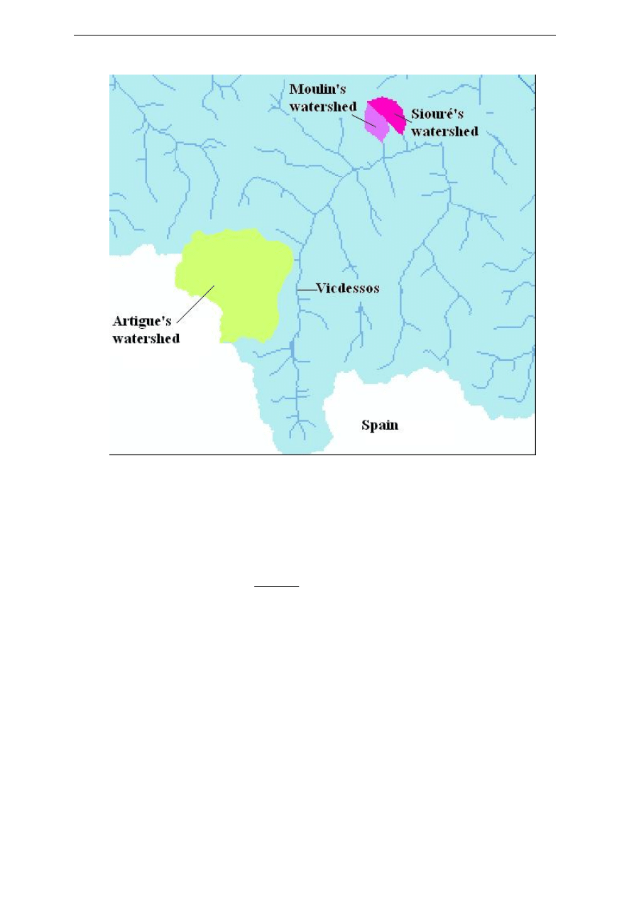
The map presented below gives a generally view of the region. The four ellipses present
locations mentioned during the entire study.

Figure 2. Locations of the different investigated points near Vicdessos. (IGN, 2006)

Caption:

1: L’Artigue, Vicdessos’ tributary, located upstream the investigated area.

2: Le Suc-Sentenac, Vicdessos’ tributary, located upstream the investigated area.

Marie Colombie exjobb 2007.9

Page 12/31

3: The studied area composed of Le Moulin and Le Siouré, Vicdessos’ tributaries.

4: Le Plateau de Beille, location of the measurement tools.

3.4 Detailed studied area

3.4.1 The

project

Figure 3. The investigated area in detail. (Sandre, 2006)

Before beginning each task, the main goal is to have details on the area and then to decide on
the position of different elements. Two streams, Le Moulin and Le Siouré, are on the same side
of the Vicdessos Valley, in the Ariège, a region in the south-west of France. A field trip permits
to assess numerous properties and characteristics of the area. The rivers run on about 2.5 km
and they are separated by 1 km. The slope is quite steep (around 50%) and the flows are very
limited.

After studying a few possibilities, the team concludes on the two following scenarios.

The only way to build a power house is at the end of Le Siouré as shown in Figure 3.
The two rivers have to be joined. Le Moulin can be diverted until the other one at two
different points according to geographical aspect. To take advantage of the slope, the
water intake should be placed at 1134m, the highest point and then a waterfall of 469m
will be created. The diversion is located in Figure 3 as blue circle called “catchment 1”.
The joining point is located as a blue circle called “catchment 2”

The second scenario is simpler. Because the diversion of Le Moulin can be interrupted
by an economical issue or an environmental issue, we have to think to harness only Le
Siouré

Power house
alt : 665 m

Catchment 1
alt : 1150 m

Catchment 2
alt : 1134 m

Marie Colombie exjobb 2007.9

Page 13/31

3.4.2 Geological characteristics

Information collected during the visit is completed by geological maps (BRGM, 2002 and
Conseil régional, 2006). They allow a good approximation of the ground state of the watershed.
It is necessary in order to complete parameters in HEC-HMS. Indeed infiltration and porosity
depend on this geological state.

Two metamorphous rocks, formed by compression, are dominating the area:

The granite is a common and widely occurring type of intrusive, felsic, igneous rock. It
contains quartz, micas and feldspath (Wikipedia, 2006). It is a non porous impermeable
rock. The water will not run easily inside.

The migmatite is based on calcite and is more permeable than the previous one.

3.4.3 Climatic and vegetation characteristics

This zone in the mountains is characterized by cold winters with snow and frost. It receives a
double influence from ocean and the Mediterranean. This influence is observed on the flora
maps. The investigated watershed is shared in three zones depending on altitude. At low
height, there is a lot of vegetation such as fern. The place is still wild and the agriculture is in
decline in this region. The interim part is quite mixed and characteristic from granite ground.
Then, the superior part is narrow with specific grass. Interception and evaporation are not
insignificant and prevent the water from a rainfall to reach the soil and feed the rivers.

In spite of this data, it is quite poor to conclude on porosity and an infiltration value. Some
assessments have to be done to use the software.

3.5 First estimations

With a first estimation of the mean flow, the mean power can be estimated. With a mean flow
value of 0.1 m

/s, the power formula can be applied.

(1)

η: the total efficiency (~0.90)

g: the earth acceleration (m.s

-2

)

Q: the estimated flow (m

/s)

: The effective height= the real height minus the loss in the penstock

(0.9*DeltaH = 0.9 * 469 = 422m)

ρ: water density (kg/m

)

This calculation estimates the power to 380kW. At this step of the study, the representatives
already know that they will be able to produce hundreds of kilowatts. This value is quite
underestimated with a very small flow and a high head pressure loss inside the penstock.

Marie Colombie exjobb 2007.9

Page 14/31

4 GIS WATERSHED DELINEATION

GIS watershed delineation is the first step to begin a hydrological study. The surface of the
basin is needed to determine all the values and to use the software, HEC-HMS.

4.1 The definition of a watershed

A watershed, or a water catchment is a specific area which can be defined for each point on the
Earth. This limited area represents the surface where a drop could fall to join the investigated
outlet by draining and running off. Figure 4 shows the boundaries of the watershed for the main
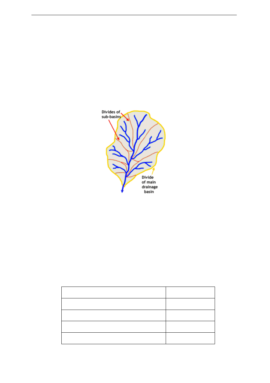
river and also sub-basins for each affluent. The yellow line corresponds to the ridge line.

Figure 4. Watershed description. (Wikipedia, 2006)

4.2 GIS: the geographical information system

The geographical information system is highly present in hydrological and hydraulic studies.
Certain software such as Arcgis or MapInfo is able to calculate watershed areas based on
specific maps which contain altitude information. In this report, the results are provided by
Arcgis. The basin work maps were consulted at the Fluid Mechanics Institute of Toulouse
(IMFT) and allow calculating different areas mentioned in the following table. Le Suc-Sentenac
and L’Artigue are different rivers which will appear during the study. They are described in the
next part of the report. Figure 5 shows the graphical result given by Arcgis.

Table 1. Surface values for the different watersheds.

Watershed’s name

Areas (km

)

Le Moulin

at the intake point (“catchment 1”)

2.47

Le Siouré

at the intake point (“catchment 2”)

2.92

Le Suc-Sentenac

24.8

L’Artigue

Marie Colombie exjobb 2007.9

Page 15/31

Figure 5. Watersheds bounderies drawn by ArcGis simulation.

These values are very useful for the entire project. For example, they allow comparing the
different watersheds by calculating a specific flow Q

. Because its unit is in l/s/km

, the

comparison between two rivers does not consider the surface or the length of the streams. This
specific flow is calculated with the mean annual value Q

/s). Q

is often ranged between 20

and 45 l/s/km

. The calculation formula is following.

1000

[

l/s/km

] (2)

Marie Colombie exjobb 2007.9

Page 16/31

5 METHOD 1: A HYDROGRAPH BASED ON STATISTIC

ANALYSIS

5.1 Collection of the most relevant data

Until today, no gage is placed on the two streams and so, no data has been measured. In order
to calculate the natural flow, a statistical analysis has to be done on other surrounding rivers.

As seen in Figure 2, Le Suc-Sentenac (n°2) is on the same side of the valley. On a field trip, a
very high similarity was observed between the two basins (n°2 and n°3). The project assesses
that there is just a difference of catchment area. EDF (French electricity supplier) has monthly
average data between 1961 and 1995 for Le Suc-Sentenac. Thanks to this information and
Arcgis results, a specific flow value is determined around 30 l/s/km

. Then, the same value can

be used for the chosen area.

Unfortunately, the monthly averages are not sufficient to determine the most relevant value of
the harnessed flow. Moreover, to study the heterogeneity of the flow repartition each month,
daily data should be calculated.

The solution is to study another river: L’Artigue (n°1 in Figure 2). It is located around 10
kilometres to the south-west direction of the chosen rivers. Thanks to Hydro Banque, Artigue’s
daily averages on forty years are available. It represents a reliable source to calculate and
extrapolate statistical results. Indeed, more than thirty years data is manna for hydrologists.

However, because the side exposition is different, it has a different reaction to the rain, the
snow and the sun. The source is at a totally different place. So the specific flow is totally
different, around 54.8 l/s/km

, i.e. almost a double value. It is not possible to assimilate directly

Artigue’s watershed with the studied basin.

So, the first step of this statistical method is to find a correlation between L’Artigue and Le Suc-
Sentenac

thanks to specific flows. Then, I will be able to transfer calculated data to analyse the

two streams at a second step.

5.2 Frequency flow diagram

The frequency flow graph is essential to develop mini-hydro. It is used to estimate different
scenarios of rated power and also to calculate the compensation flow whose notion is explained
in the section 5.3. This graph represents the number of days in one year when a certain flow or
a superior flow occurs.

Marie Colombie exjobb 2007.9

Page 17/31

5.2.1 The correlation analysis between Le Suc and L’Artigue

This correlation has to be found to correlate the Suc’s behaviour and the Artigue’s behaviour.
By using specific monthly flows made over several years, the following graph is drawn.

Figure 6. Linear correlation between L'Artigue and Le Suc-Sentenac.

A strong correlation is directly predictable. Indeed, a line can be drawn with all the points. With
Excel, a r-square value is calculated and equal to 0.94. This value is evidence of the statistical
relationship. It is very high and so confirms the first assessments. Then a linear equation (3) is
obtained. It allows to establish discharge frequency relationships for the two rivers.

2.29

)

014

(

Art

Suc

[

/s]

(3)

Only one recommendation has to be made for the application of this equation. The equation is
not valid for very low flow values (<0.1m

/s).

5.2.2 The Myer formula

The Myer formula (4) allows estimating flows thanks watersheds surface values if the rivers are
similar such as Le Moulin, Le Siouré and Le Suc-Sentenac.

[ ]

Q =

(4)

« α » is a regional coefficient. It can generally vary between 0.5 and 1 depending of the
watershed’s shape and the slopes. According to different French hydrologic studies, 0.72
seems to be the most relevant value. This 0.72 will be used during the entire subsequent study
(D.MOSNIER, 2006).

y = 2.2899x - 14.036

= 0.9438

100

120

140

160

180

Qs Suc (l/s/km

)

Qs Artigue (l/s/km

)

Marie Colombie exjobb 2007.9

Page 18/31

For example, monthly average values can directly be determined for the association of the two
investigated streams (S

=2.47+2.92=5.39km

) at the joining point thanks to the Suc’s values

=34km

Table 2. Monthly averages calculated by the Myer formula

Month January

February

March

April

May

June

Suc flow (m

/s)

0.50 0.56 0.72 1.27 2.32 2.44

Investigated flow (m

/s)

0.13 0.15 0.19 0.34 0.62 0.65

Month July

August

Sept

October

November

December

Suc flow (m

/s)

1.26 0.65 0.59 0.67 0.67 0.59

Investigated flow (m

/s)

0.33 0.17 0.16 0.18 0.18 0.16

The mean value is also calculated at 0.27 m

/s.

With the same method a table for Le Siouré is build with an annual average value of 0.16 m

/s.

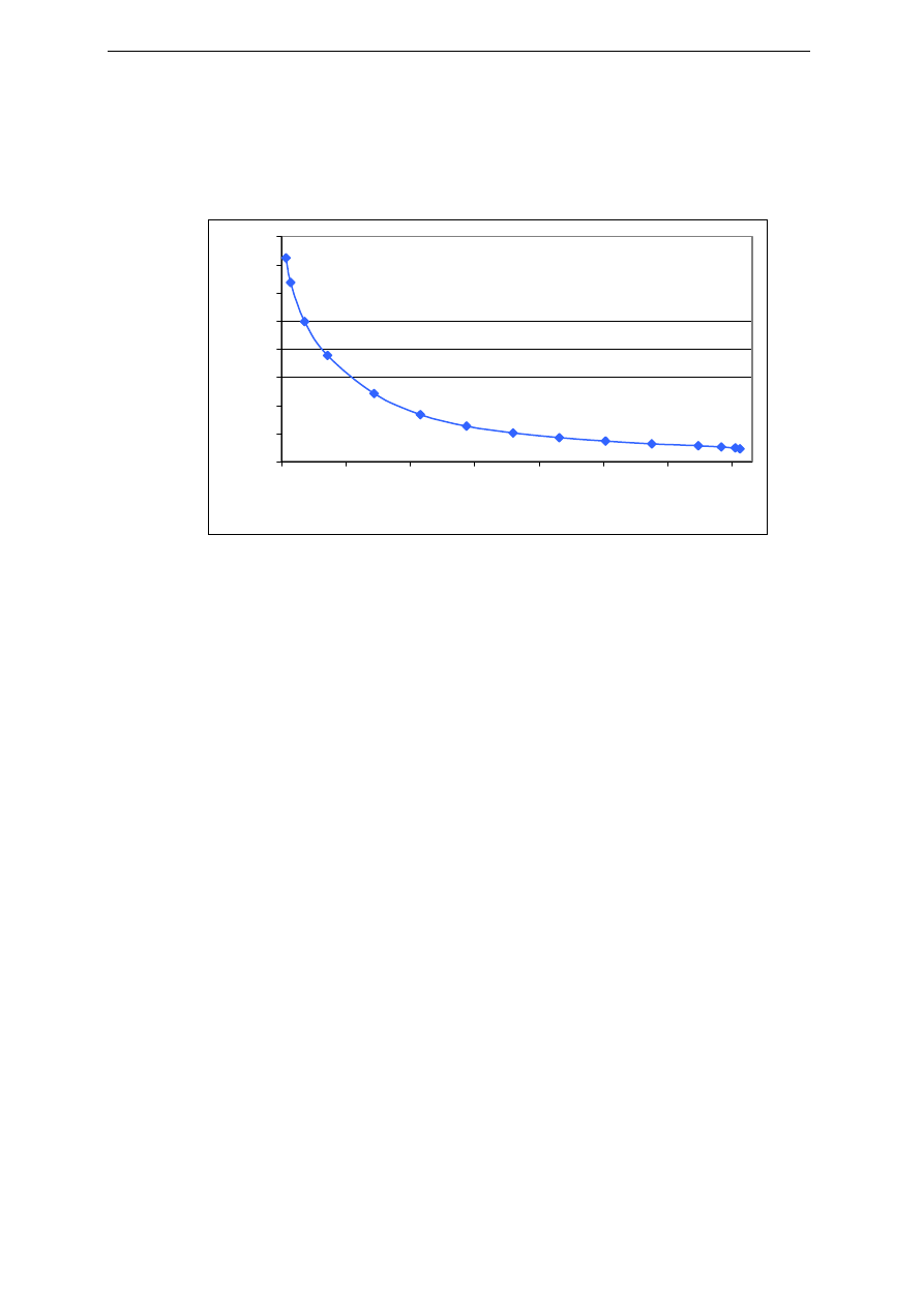
5.2.3 The frequency flow diagram

Now, all the elements are brought together to build a frequency diagram. Forty years of daily
data allow statistics about the frequency of certain flows for L’Artigue. Some statistical functions
in Excel allow knowing the value which corresponds to a percentage of the entire data base
(CENTIL). By changing the percentage in number of days, I obtain the most useful graph for a
hydrologist.

Then applications of the equation (3) and the Myer formula (4) offer the following graph in
Figure 7. It is a very good way to explain the situation of a river. For example, it shows that a
flow over 0.4m

/s is observed 72 days in a year. Of course, it is not always the same and that

provides just an average. These values will change for a dry year, or a wet year. However,
because the project is planned for at least 40 years, all hydraulic studies use this relevant and
interesting graph.

Figure 7. Frequency flow diagram representing the association of the two rivers.

0.0

0.2

0.4

0.6

0.8

1.0

1.2

100

150

200

250

300

350

Days number

Flow Moulin+Siouré (m

/s)

Marie Colombie exjobb 2007.9

Page 19/31

As mentioned before, I have to be careful during the study. The deviation of Le Moulin is
perhaps not possible because it could be too expensive or forbidden by environmental
agencies. It is why the water resource of Le Siouré alone is also studied. With approximately the
same method, and a different surface value, a hydrograph and a frequency flow diagram can be
drawn as showed Figure 8.

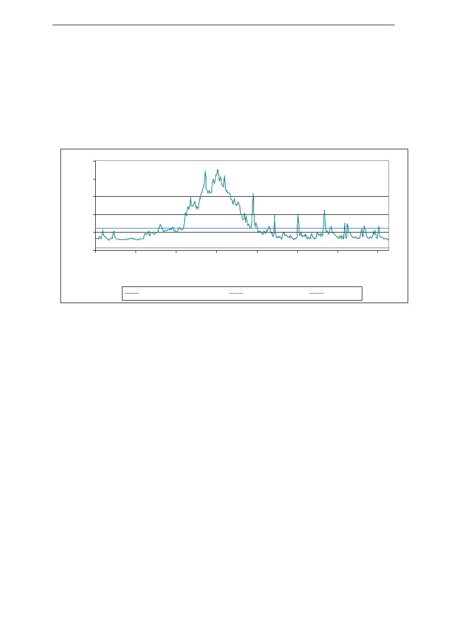
Figure 8. Flow frequency diagram for Le Siouré.

At this phase of the study, the hydrologist, in collaboration with the powerhouse owner and the
financial expert, is able to determine the more relevant scenarios. It depends considerably of
the strategy which the owner wants to apply. For example, for a very hazardous strategy, a
small number of days can be chosen to produce a high amount of electricity during a short
period of time each year. However, because the hydrograph varies each year, the owner has to
be sure he or she can wait for a few years before beginning a profitable phase. The only
company capable of taking such a risk is EDF with enormous dams in the Pyrenees and the
Alps. For this precise situation, the most relevant strategy is less hazardous with a period of
production more important.

Before giving numbers and figures a compensation flow has to be calculated, based on the
previous graph.

5.3 The Compensation flow

In many countries, the law obliges letting a minimum rate flow in the river for ecological
purposes. It allows the aquatic life to continue reproduction of the species. This flow is called
compensation flow, Q

. It is calculated with a nominal flow (Q

) which corresponds to the flow

value observed at least 120 days during a year (Q

=1/10 Q

). The diagram built before is very

useful to determine Q

. The calculation gives 25l/s.

To conclude, the municipalities have to let 25l/s in the natural river bed. Moreover, if the
diversion can not be done, I estimate also a compensation flow for Le Siouré at 16l/s.

In order to illustrate the result of the analysis, a first scenario could be a duration of 110 days
per year. The associated flow is 0.27 m

/s. When the flow is superior to this value, the excess

flow does not go through the turbine, and runs directly to the natural riverbed. When the flow is
below this limit, the owner can produce electricity; however, the yield of the turbine is less good.

0.0

0.1

0.2

0.3

0.4

0.5

0.6

0.7

0.8

100

150

200

250

300

350

Days number

Siouré's flow (m

/s)

Marie Colombie exjobb 2007.9

Page 20/31

The specialist of hydraulic power plants will fix a minimum flow to stop the turbine and avoid a
loss of energy. By subtracting the compensation flow, nominal powers is assessed for

Scenario1:

=0.90

9.81

(0.27 – 0.025)

422

1000 = 913kW and for

Scenario2:

=0.90

9.81

(0.17 – 0.025)

422

1000 = 540kW

Marie Colombie exjobb 2007.9

Page 21/31

5.4 Hydrograph

The hydrograph enriches also the work to study the variation each day. In the mountains, it is
very characteristic. The snowmelt feeds the rivers during the spring. At the opposite side, the
winter level is very low because snow replaces rain. The team which studies in details the
profitability needs this information to compare the price of electricity sell and the different
scenarios. This graph is obtained by the translation of Antigua daily values based on the
averages of the 40 years of data.

Figure 9. Flow average variations made over forty years.

0.0

0.2

0.4

0.6

0.8

1.0

01-janv

20-févr

11-avr

31-mai

20-juil

08-sept

28-oct

17-déc

Days

Flow (m

)

Moulin+Sioure hydrograph

Compensation flow

Q110days

Marie Colombie exjobb 2007.9

Page 22/31

6 METHOD 2: HEC-HMS, PRECIPITATION-RUNOFF MODEL

The Hydrologic Engineering Center’s Hydrologic Modelling System (HEC-HMS) is capable of
simulating the precipitation-runoff processes of watershed systems. It allows an application in a
wide range of geographic areas. This includes large river basin water supply and flood
hydrology, and small urban or natural watershed runoff. For the basin located in the mountains,
HMS is able to simulate snowmelt and runoff on hard slopes. Hydrographs produced by the
program are used for studies of water availability, urban drainage, flow forecasting, future
urbanization impact, reservoir spillway design or flood damage reduction.

The software offers several possibilities and mathematical models for representing each flux.
Each mathematical model is suitable in different environments and under different conditions.
Making the correct choice requires knowledge of the watershed, the goals of the hydrologic
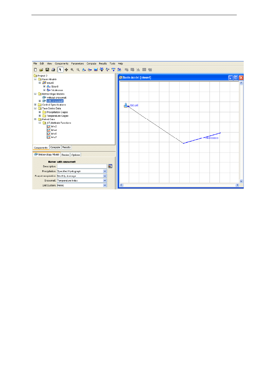
study, and engineering judgment. An example of the interface of the program is showed in
Appendix 1.

My first goal is to learn how to use this software. Understanding the different methods and the
necessity of each value is very important to criticise results and to have the benefit of hindsight.
Afterwards my command of the software could allow me to revaluate some values and to adapt
some specific situations. Because the statistical result seems very satisfying, a narrow parallel
between it and the HEC-HMS results will be done at each step.

6.1 Data collection

The main data required to use HEC-HMS is rainfall patterns. The period of record simulation
required the input of daily rainfall totals. Unfortunately most rainfall gages are manual near our
investigated area. It involves that there are missing periods of data. Thus the hyetograph is
build based on a rainfall gage on Le Plateau de Beille, at 10 km in the east direction. This
precipitation gage depends on ASTON and is named Plateau de Beille with the code 09024004
(Base Sandre, 2006). It is placed at 1790 m and is located with the Lambert coordinates at the
point (547;1747.1). The location is showed by n°4 in Figure 2. It is an automatic station with
delayed transmission. Then it is certain that the record is correct and useable. The following
study is based on 2005. The main interest in to compare the statistical hydrograph with different
HEC-HMS models. For that, I will focus on Le Siouré on one year. As expected, another
hydrograph is drawn by statistical way to take only 2005 in count.

Moreover this meteorological station gives data for evapotranspiration and also registers
temperatures by making an average each day with the minimum and the maximum of
temperatures. These two parameters are necessary to model specific criteria explained later.

6.2 General model in the software

After entering known geographical parameters in the software, several calculation methods
have to be chosen and criteria have to be estimated cleverly. These methods are presented
below.

6.2.1 Overland flow model: SCS unit hydrograph

The overland flow is essential to model a watershed. It represents the flow of water over the
ground before it enters the stream (International Glossary of Hydrology, 2006). Several methods
are proposed in the software. Unfortunately, the lack of data obliges to choose only one: SCS
unit hydrograph. Even if it is not the most precise, the criteria used are known.

Marie Colombie exjobb 2007.9

Page 23/31

The method is based on an analysis of small watersheds used for agriculture. It uses a delay
time, called Lagtime which characterizes the time between the rainfall and the flow peak in the
river. For most of the cases, this value is estimated by taking 60% of the concentration time.
This is the period of time required for a drop to run to the outlet from the point of a drainage
basin having the longest travel time (CHOW, 1998). Thus, by using 0.75m/s for the drop speed
and 4.7 km for the watershed length, the Lagtime is estimated at:

0.6*4700 m /(0.75m/s*60) = 63 min

6.2.2 Loss model: Deficit and constant

According to the geological criteria, “Deficit and constant” is the most relevant method to model
the ground of the investigated watershed. It creates a unique ground cover characterized by a
constant infiltration loss rate and an initial and maximum deficit to simulate the wetting and
drying out process.

Initial deficit

is a value considering initial conditions in the soil, i.e. quantity of water already

present in the ground at the beginning of the simulation in mm. Arbitrarily, 40% of the maximum
storage is chosen (HEC-HMS user’s manual, 2006). It is ranged from about 2.5 to 25 mm
(Mississippi flow frequency study, 2003).

Maximum storage

is the retention capacity of the ground in mm. HEC-HMS user’s manual

proposes to calculate it with the product of the porosity and the depth. Then, 135mm is found. It
involves a high initial storage which could be changed during simulations.

Impervious

is a percentage of impervious zone. Zero is chosen because the land is not

occupied by humans building.

Constant rate

in mm/hr is an infiltration speed whereas the maximum storage is reached. No

data is available to assess this kind of value. Consequently, several simulations are done to
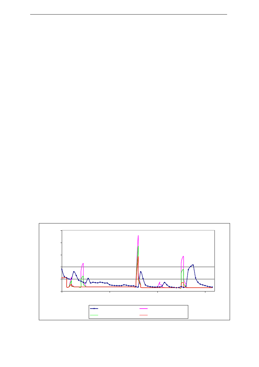
select the best one. Figure 10 shows on a short period of the hydrograph for three different
constant rates and the statistical simulation in blue. Undoubtedly, an ability to vary the rate by
months or by reasons would improve the simulation. However some references generally give
constant infiltration looses of about 0.5 mm/hr (Mississippi flow frequency study, 2003).

Figure 10. Infiltration rates influence on the hydrograph.

0.0

0.2

0.4

0.6

0.8

1.0

29/06/2005

19/07/2005

08/08/2005

28/08/2005

Flow m

statistical model

infiltration 0.2 mm/h

infiltration 0.5 mm/h

infiltration 0.8 mm/h

Marie Colombie exjobb 2007.9

Page 24/31

A low infiltration rate (pink line) involves too much overland flow and induces too high peaks on
the graph. At the opposite side, a high infiltration rate (red line) is too invariant except for the
beginning of August. However the most judicious choice seems to be between these two. An
intermediate value allows to simulate several peaks not too high. Thus simulations are always
running with 0.5 mm/hr.

6.2.3 Underground flow model: Baseflow monthly average.

The software allows to answer to each rain events. However, the river keeps on running even if
it does not rain. It is why the model needs a minimum flow value, corresponding to groundwater
resources. Normally these estimations are based on minimum monthly flow values at various
gages sites. Once again, no historical data are available. It is why the only solution is to use the
statistical model. For each month, I took the minimum data observed in the new statistical
hydrograph.

Table 3. Baseflow choices for each month in l/s.

JAN FEB MARCH APRIL MAY JUNE JULY AUG SEPT OCT NOV DEC

54 50 49 92 234 221 71 59 58 58 58 49

6.3 Limits of the simple model

All the based criteria are now determined and allow first simulations. It is very obvious to
observed that this simple model has limits because it does not use the specificity of the studied
area.

Indeed, a first remark could be the too high peak values. The software uses all the rainfall
volume and distributes it between infiltration and runoff, as a field without vegetation. However,
as seen during the field trip, the entire watershed is covered by dense forests. The leaves
intercept a percentage of drops.

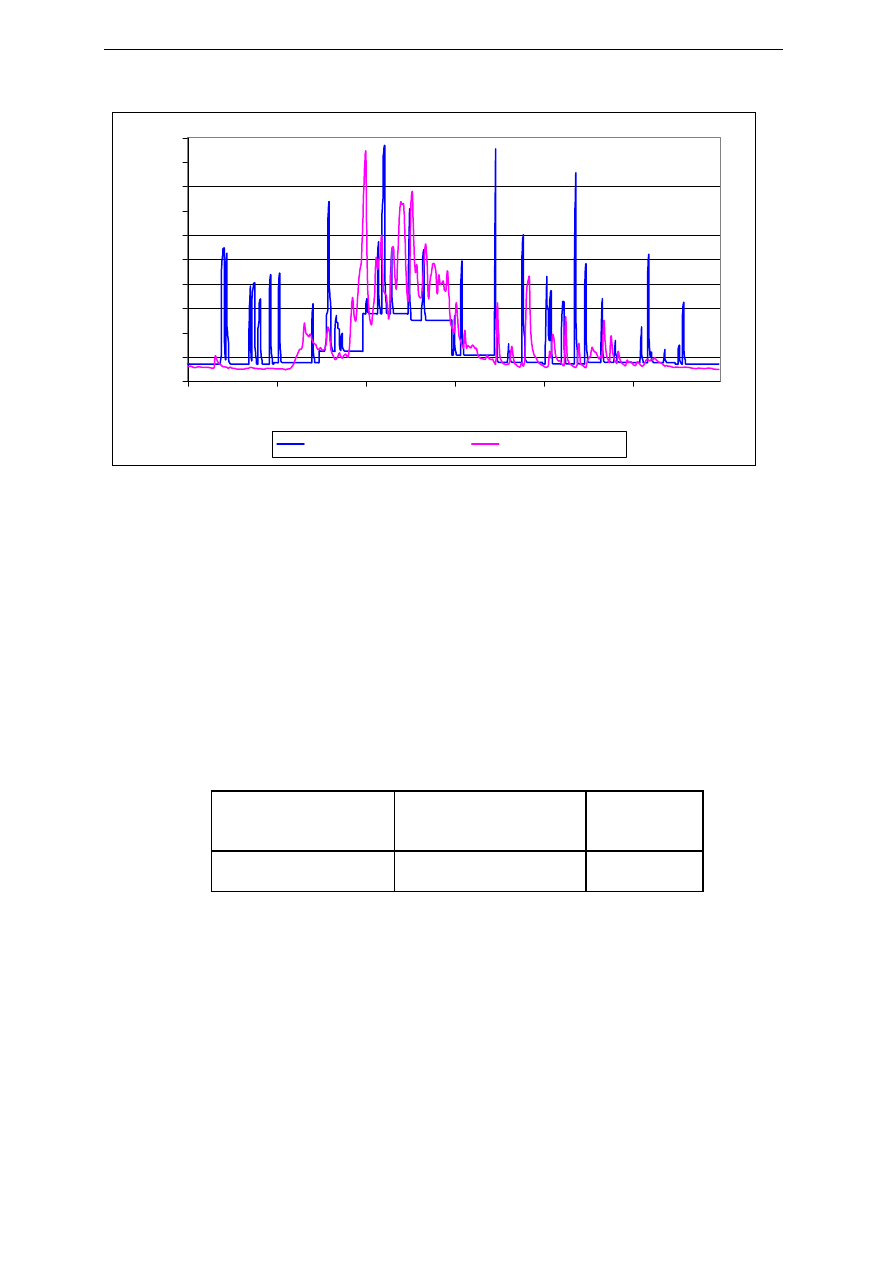
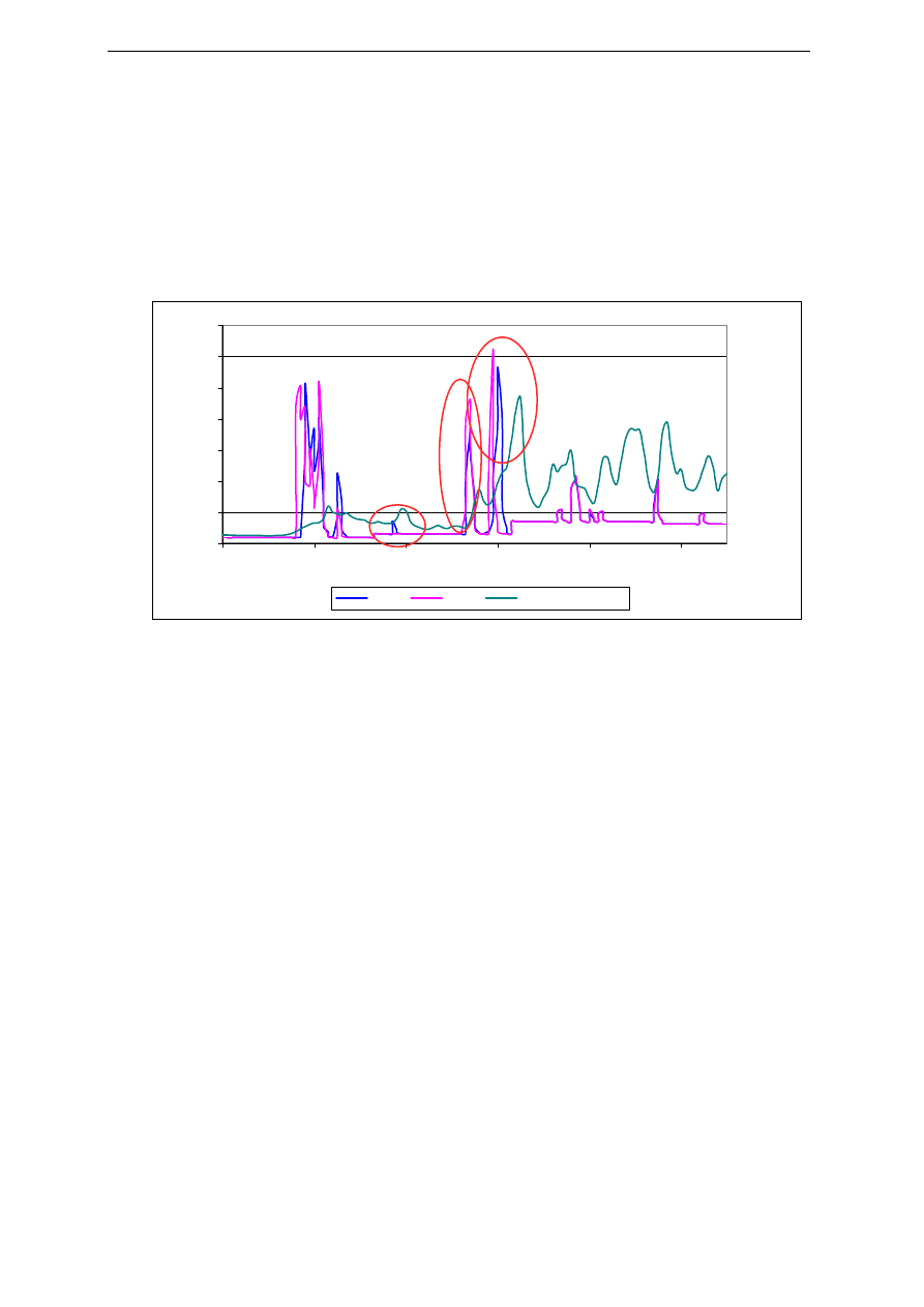
Moreover another problem is met here. The Figure 11 presents the results obtained with the
statistical study and the results simulated by HEC-HMS. It is very easy to observe a good
correlation of the flow peaks between July and end of November. Because it is not snowing
during this period, the model reacts to the different rainfalls as well as the statistical hydrograph.
However, the beginning of the hydrograph does not correspond to the real case. Indeed, without
a snowmelt model, the software reacts in one hour to each rainfall events instead of creating
some kind of reservoirs to collect snow which will melt during the next spring.

Marie Colombie exjobb 2007.9

Page 25/31

Figure 11. Comparison of the statistical model and the HEC-HMS simulation.

In conclusion two specific criteria have to be defined and used for the simulations:
evapotranspiration and snowmelt.

6.4 Evapotranspiration

Evapotranspiration is a very important part of the water cycle. It is necessary to better know the
watershed behaviour. It corresponds to the sum of evaporation and plant transpiration. When it
is raining, vegetation intercepts water drops and uses it to grow. At the same time a loss of
water occurs by evaporation of a lake or the soil (Wikipedia, 2006). Data is available thanks to
MétéoFrance (meteorological French service). Table 4 presents the average values to show the
quantity of evapotranspiration compared to rainfall volume.

Table 4. Total evapotranspiration and rainfall values for 2005 (Météofrance, 2006).

Rainfall value in 2005 in

Evapotranspiration in

2005 in mm

Percentage

811.3

639.7

The average annual precipitation over the basin is 810 mm. Of this amount, an estimated 640
mm returns to the atmosphere by means of evaporation and transpiration, i.e. 79%. These
values confirm that this phenomenon is not negligible, specially in this region with dense forests.

Thanks to the gage placed in Le Plateau de Beille, I collected one value of evapotranspiration
for each day of the 2005 year. Thus, I enter monthly averages in HEC-HMS and I obtain new
simulations.

6.5 Snowmelt

The two investigated streams are in the Pyrenees and have an origin around 1940m. The snow
has a very important influence on the hydrograph. There is a delay between the snow

0.1

0.2

0.3

0.4

0.5

0.6

0.7

0.8

0.9

01/01/05

03/03/05

03/05/05

03/07/05

02/09/05

02/11/05

Flow (m

/s)

HEC-HMS simulation

statistical model

Marie Colombie exjobb 2007.9

Page 26/31

precipitation and the flow feeding. This quantity of water is not minor. To model that, a lot of
characteristics have to be determined. For considering snowmelt, a hydrological year is defined
to begin the animation the first September. Thus it is sure that there is no snow at the beginning
of the simulation.

For that, two categories of values are needed. First the threshold values create boundaries
between rainfall and snowfall events. For this case study, values are interpreted or copied in
hydrology previous studies. Then a snowmelt model gives a formula to simulate this
phenomenon.

Main threshold values

Px : base temperature below which there is snow instead of rain.

Base Temp : base temperature above which snowmelt occurs.

Wet melt rate : Snowmelt speed when it is raining.

Ati melt rate : Time interval between two rainfalls.

Water capacity : maximum water quantity which snow can retain before running off.

Table 5. Chosen criteria for the snowmelt model.

Criteria Value

0°C

Base temperature

1°C

Wet melt rate

2 mm

Ati melt rate

0,98

(HEC-HMS user’s manual, 2006)

Water capacity

(HEC-HMS user’s manual, 2006)

Temperature index-method

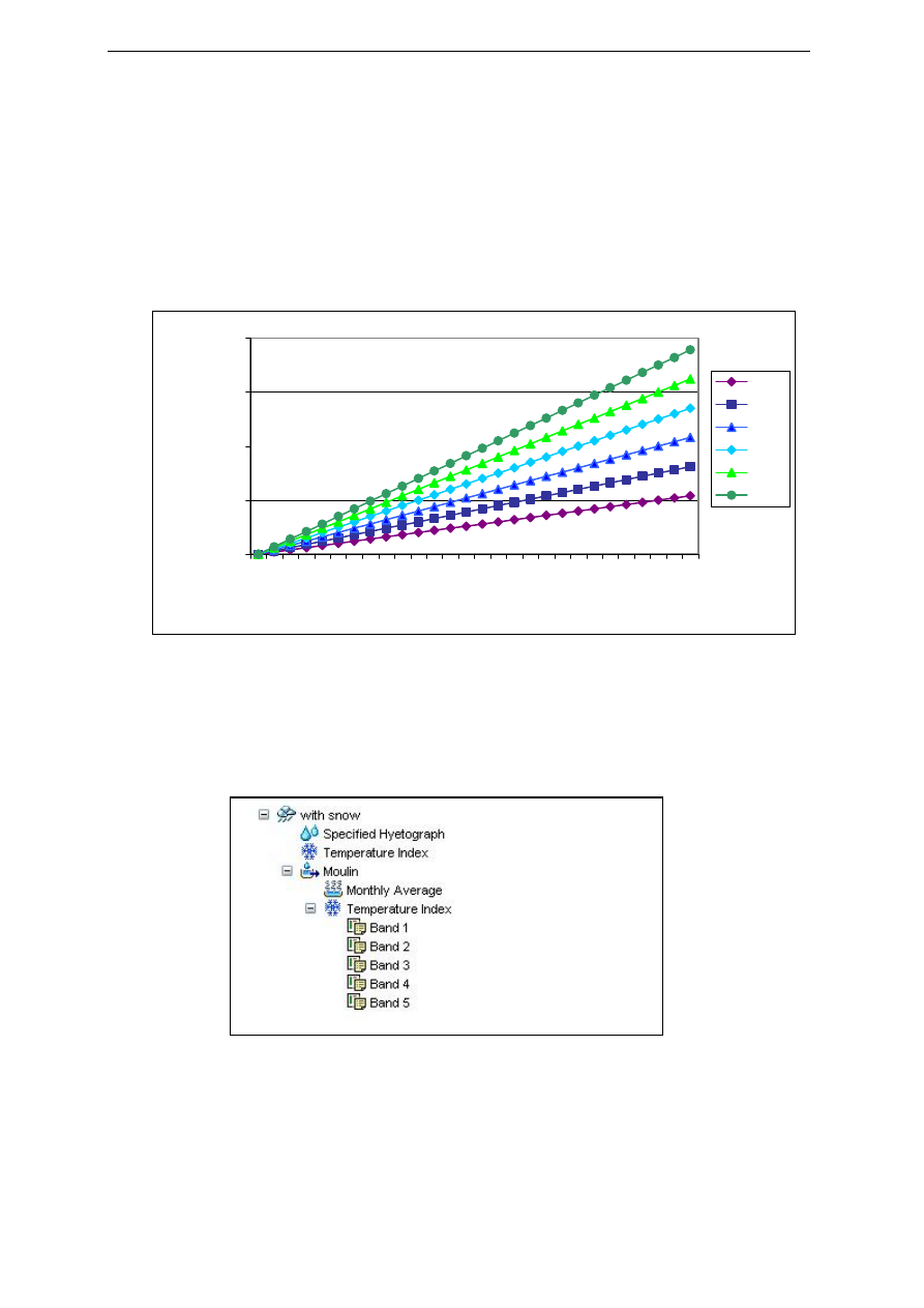
The Paired Data function in HEC-HMS allows entering a formula to express the snowmelt
speed. Based on the concept that changes in air temperature provide an index of snowmelt, this
model was developed by Jaroslav Martinac in 1975 in small European basins. It is simple but
specially made to forecast daily stream flow in mountain basins where snowmelt is a major
runoff factor. Equation (5) indicates Martinac’s formula and Figure 12 shows the seven different
models which could possibly be used for the temperature index method.Needed data is
principally air temperature:

Measured meteorological daily values collected by Meteofrance.

Secondary meteorological variable that provides an integrated measure of heat energy.

Marie Colombie exjobb 2007.9

Page 27/31

)

-T

(5)

M = snowmelt (mm/day)

Mf = degree day factor (mm/°C/day)

= air temperature (°C);

= threshold or base temperature above which snowmelt occurs (°C).

Figure 12. Different snowmelt models based on Martinac 's theory.

Only one temperature is available for each day. However, we can observed very different
temperatures at the same time in different parts of the area, depending on the altitude. It is why
a division of the watershed in five parts is made between 1134m and 1899m. Majority of the
time we can say that we loose 0,7°C each 100 m of altitude (MOSNIER, 2006). Figure 13
shows the interface of the software with the definition of each bands.

Figure 13. Parameterisation of the five alti-zones.

100

150

200

Temperature (°C)

Melted snow quantity (mm/°C/day)

Mf=2
Mf=3
Mf=4
Mf=5
Mf=6
Mf=7

Elevation n°1: 1219 m
Elevation n°2: 1389 m
Elevation n°3: 1559 m
Elevation n°4: 1729 m
Elevation n°5: 1899 m

Marie Colombie exjobb 2007.9

Page 28/31

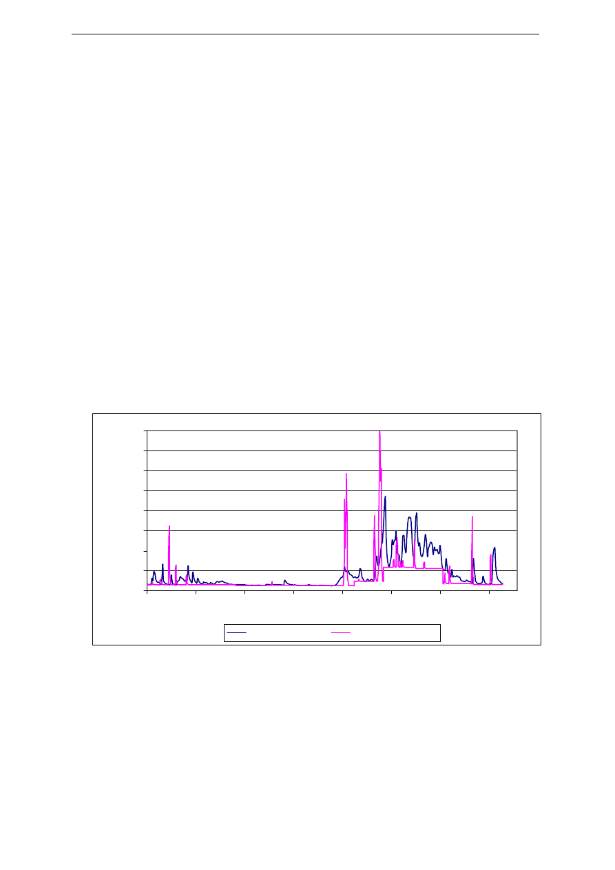
To choose the most relevant mf coefficient, I process several models. Figure 14 illustrates the
difference between mf=2 and mf=7. Even if the difference is not so obvious, the model mf=2 is
more satisfying. By taking the three circles from the left to the right, we can make three remarks
during the snowmelt period. The first one shows that only mf=2 simulates a peak at the
beginning of April. For the second circle, we can see that the pink peak is higher than the blue
one. So it is very far from the statistical model. Then, the last circle shows that the pink peak is
too early compared to the blue one and to the statistical one. In conclusion, mf=2 is chosen for
HEC-HMS criteria.

Figure 14. Snowmelt coefficient influence on the hydrograph.

0.2

0.4

0.6

0.8

1.2

1.4

27/02/05

19/03/05

08/04/05

28/04/05

18/05/05

07/06/05

Flow (m

/s)

mf=2

mf=7

statistical model

Marie Colombie exjobb 2007.9

Page 29/31

7 FINAL RESULTS

The goal of this last part is to compare the different results. By talking with hydrologists and
professors, I understood that statistics are often used for this kind of problem. Because too
many data are missing, it is obvious that the statistical hydrograph gives the best result.
However some specific problems could appear by the comparison of this graph with HEC-HMS
results. I can detect a problem with the statistic or the software. Anyway the similarity between
the graphs could at least confirm a good parameterisation of the software.

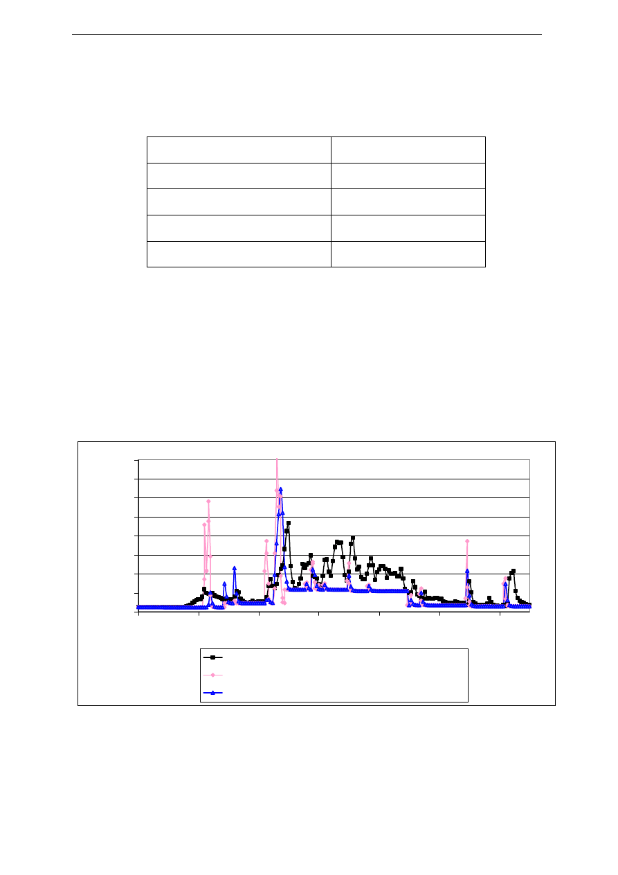
After the entire study, the two different ways lead to figure 15. A first observation allows a
feeling of satisfaction. Peaks are correlated and mean values correspond approximately
(statistic mean=0.162m

/s and HEC-HMS mean=0.116m

/s). I can already confirm that it was

not ambitious to take data from rivers downstream or rainfall patterns on the neighbour valley.
The hydrological regimes show a river located in the mountains with a clear separation of the
seasons. Besides, a small remark has to be done here: the present hydrograph is calculated for
a hydrologic year, i.e. from first September to 31 August. In the first place, it is sure that the
HEC-HMS simulation begins without snow. Secondly, it is generally the way of hydrologists to
work.

However the pink peaks are especially high. The model of a unique soil cover can maybe be
accused. More geological data could be precious to have a better simulation. We can also think
that the statistical way mitigates maximal values.

Figure 15. Final comparison of HEC-HMS and statistic for Siouré's hydrograph.

Two anomalies are easily detected by the comparison of the two graphs. Two peaks appear
around 19

March and 21

April. In the statistical study values are lower. Despite a change of

specific criteria such as maximum storage which can allow more infiltration, peaks seem to be
still very high. By observing in detail the temperature variations, the origin of these perturbations
are rapidly detected. Indeed only one temperature is registered per day. It consists in the
average of the minimum and the maximum observed during the day. It is easy to understand
that it is not the best way to process. Unfortunately, it is the only one in this case. So the HEC-
HMS model simulates a uniform temperature during 24 hours. In reality it is totally different with

0.0

0.2

0.4

0.6

0.8

1.0

1.2

1.4

1.6

01/09

21/10

10/12

29/01

20/03

09/05

28/06

17/08

Flow m

statistical model

HEC-HMS model

Marie Colombie exjobb 2007.9

Page 30/31

cold night and very heterogeneous temperature during the day. Table 6 shows the temperature
before and during the second anomaly.

Table 6. Entered data for temperature variations during an anomaly.

Date Temperature

19 April 2005

-1,8°C

20 April 2005

1,3°C

21 April 2005

6,3°C

22 April 2005

8,0°C

During two entire days temperature is registered above 6°C whereas the base temperature
above which snowmelt occurs is only 1°C. Then, it is easy to understand the peak. When the
snowmelt model is not chosen, this problem does not exist. Temperature values are normally
requested several times per day. Consequently the simulated period of HEC-HMS simulation
could not closely match the statistical hydrograph. This reflects a lack of data. To confirm my
assessment, I decide to reduce the temperature without changing anything else. Figure 16
shows in blue the new model. The first peak totally disappears while the other one is reduced
from 1.74m

/s to 1.29 m

/s. In the same time, the statistical value of the peak just following is

0.94m

/s. The percentage of error is reduced to 47%. In conclusion, more precise temperature

data is needed to complete the HEC-HMS model.

Figure 16. Influence of temperature data changes on the peaks in the hydrograph.

0.0

0.2

0.4

0.6

0.8

1.0

1.2

1.4

1.6

17/02

19/03

18/04

18/05

17/06

17/07

16/08

Flow (m

/s)

statistical model
snowmelt model
snowmelt model with changed temperatures

Marie Colombie exjobb 2007.9

Page 31/31

8 CONCLUSION

Thanks to several specialists met during these last months, we know that the water resource
can be estimated, in this case, by the statistical analysis. It is a good way to have estimations
and to do some scenarios for the power plant, when there is no specific data on the investigated
streams. However, it is not sufficient to begin the construction work. We have, at least, to place
one or two flow gages during one year to confirm the hydrograph and then to be sure about the
viability of the frequency flow diagram.

The HEC-HMS part was more useful to learn how to command this precious software. The work
of calibration represents an important part of the hydrologist work and so it is very interesting for
me. However, it was a good way to detect a big error in the statistical method. Because the
peaks were often connected, the study confirms that we can use data from rivers and
precipitation gages at a few kilometres from the chosen area. This study shows also that a lack
of data is often met during this kind of work and the specialist has to use some tricky strategies
to do valuable estimations.

To conclude about the project, we can already define two different nominal power levels. They
are based on the two frequency flow diagrams for a number of days equal to 72days. That gives
1500kW

if the deviation of Le Moulin is possible and 900kW if it is not. The goals of my

colleague who studies the profitability is now to confirm these figures by calculating profit with
price of electricity and also yield of turbines chosen by my other colleague. Then we will confirm
the time necessary to pay back the loan. A first approximation gives 30 years.

Marie Colombie exjobb 2007.9

Page 32/31

9 REFERENCES

Data and map collection

Banque Hydro, EDF, station de l’Artigue, 20/10/2006
http://www.hydro.eaufrance.fr/Traitement/Synthese.php?StaCode=O1115010

Base Sandre : precipitation gage information, 01/10/2006
http://sandre.eaufrance.fr/geoviewer/index.php
http://sandre.eaufrance.fr/REF/PLUVIO/09024004

Cartes géologiques du Bureau de Recherche Géologique et Minier (BRGM, 2002):
Vicdessos (1/50000)

Conseil régional de l’Ariège, cartes géologiques, 20/10/2006
http://www.cg09.fr/v2/index_service.asp#

Hola Andorra, 08/12/2006
http://www.hola-andorra.com/arinsal/pics/ariege4.gif

Institut géographique national français, IGN: 01/10/06
http://www.geoportail.fr/index.php?event=DisplayCartoVisu&url_insert=454c8017cd9addec9f7d
2e88aa8ee6ae

METEOFRANCE, La Climathèque
http://climatheque.meteo.fr/okapi/accueil/okapiWeb/index.jsp

Bibliography
British hydropower association, “Mini-hydro: a step-by-step guide”, 2006

V.Te.CHOW, D.R.MAIDMENT, L.W.MAYS, « Applied hydrology », 1998

G. DEGOUTTE, Comités français des grands barrages, « Petits barrages »
Cemagref edition 2002

HEC-HMS, Hydrologic Modeling System, 23/11/2006;
http://www.hec.usace.army.mil/software/hec-hms/

HydroCAD, Understanding hydrology, 23/11/2006; http://www.hydrocad.net/6166b.htm

International Glossary of Hydrology; http://www.cig.ensmp.fr/~hubert/glu/EN/GF0872EN.HTM

D.MOSNIER, EDF, “Ingénierie des aménagements hydrauliques”, 2006

Upper Mississippi River System Flow Frequency Study, Hydrology and Hydraulics, nov 2003

Wikipedia
http://en.wikipedia.org/wiki/Drainage_basin 25/11/2006
http://en.wikipedia.org/wiki/Evapotranspiration 13/12/2006

Software
Arcgis®: Geographical Information System: ArcMap, ArcCatalogue, ArcView

Hec-HMS®: Hydrologic Engineering Center’s Hydrologic Modeling System: US Army corps of
engineers.