The University of California at Berkeley

April 2001

Implementation of an Active Suspension, Preview

Controller for Improved Ride Comfort

by

Mark D. Donahue

B.S. Boston University, 1998

Research Advisor:

Professor J. Karl Hedrick, Ph.D.
Mechanical Engineering

Second Reader:

Professor Kameshwar Poolla, Ph.D.
Mechanical Engineering

Submitted to the Department of Mechanical Engineering, University of California at

Berkeley, in partial satisfaction of the requirements for the degree of

Master of Science, Plan II

Implementation of an Active Suspension, Preview Controller for

Improved Ride Comfort

Copyright 2001

by

Mark D. Donahue

i

Abstract

Implementation of an Active Suspension, Preview Controller for

Improved Ride Comfort

by

Mark D. Donahue

Master of Science in Mechanical Engineering

University of California at Berkeley

Professor J. Karl Hedrick, Chair

A fully active suspension and preview control is utilized to improve ride comfort, which

allows increased traveling speed over rough terrain. Specifically, the methodology of

model predictive control has been applied to address suspension saturation constraints,

suspension rate limits, and other system non-linearities. For comparison, the following

non-preview controllers were implemented: a sky hook damping controller, a linear

quadratic regulator, and a mock passive suspension controller. Particular attention is

given to the hydraulic actuator force controller that tracks commands generated by

higher-level controllers. The complete system has been successfully implemented on a

military HMMWV using a commercially available microprocessor platform.

Experimental results show that the power absorbed by the driver is decreased by more

than half, significantly improving ride comfort.

ii

This work is dedicated to all those who have inspired

me throughout my life, with special thanks to my family & friends

iii

Table of Contents

Abstract i
List of Figures

v

List of Tables

vii

Preface viii
Acknowledgments x
Chapter 1 -

Introduction

1

1.1 Controller

Structure.................................................................................... 1

1.1.1

Low Level Control ................................................................................. 1

1.1.2

Control without Preview ........................................................................ 3

1.1.3 Preview

Control...................................................................................... 4

1.2 HMMWV

Equipment................................................................................. 5

Chapter 2 -

FTC Design

6

2.1

Overview of Controller .............................................................................. 6

2.2 Plant

Models............................................................................................... 7

2.2.1 Quarter

car.............................................................................................. 7

2.2.2 Hydraulic

actuator .................................................................................. 7

2.2.3 Complete

system .................................................................................... 9

2.3 Control

Algorithms .................................................................................... 10

2.3.1

Dynamic Surface Control....................................................................... 10

2.3.2 Output

Redefinition................................................................................ 12

2.3.3 Parameter

Adaptation............................................................................. 13

2.4 Simulation .................................................................................................. 14

2.4.1 Setup....................................................................................................... 14
2.4.2

Model Error Approximation................................................................... 15

2.4.3 Simulation

Results ................................................................................. 16

2.5 Implementation........................................................................................... 16

2.5.1 Noise

Filters ........................................................................................... 17

2.5.2

Model Error Filters................................................................................. 17

2.5.3

High-Level Control Filters ..................................................................... 17

Chapter 3 -

Subsystems

19

3.1 Safety

Systems............................................................................................ 19

3.2 Preview

Information................................................................................... 19

3.2.1 Preview

Generation ................................................................................ 20

3.2.2

Preview Sensor Correction..................................................................... 20

3.2.3 Preview

Buffer ....................................................................................... 21

iv

3.2.4

Preview Correction Modifier ................................................................. 23

3.3 Kalman

Filter.............................................................................................. 25

3.4 Performance

Criterion ................................................................................ 26

Chapter 4 -

High Level Controllers

27

4.1

Mock Passive Suspension .......................................................................... 27

4.2

Sky Hook Damping Controller................................................................... 28

4.3

Linear Quadratic Regulator ........................................................................ 28

4.4

Model Predictive Controllers ..................................................................... 29

Chapter 5 -

Experimental Results

31

5.1

Ride Height Control ................................................................................... 31

5.2

Force Tracking Control .............................................................................. 32

5.3 High-Level

Controllers............................................................................... 36

5.4

MPC Preview Controller............................................................................ 39

Chapter 6 -

Conclusions

41

References 42
Appendix A - HMMWV Hardware

44

A.1

Equipment as Received .............................................................................. 44

A.2

Sensors added by UCB............................................................................... 49

A.2.1 Servo

Amplifiers .................................................................................... 49

A.2.2

Accelerometers & Gyros ........................................................................ 50

A.2.3 Preview

Sensors ..................................................................................... 51

A.3 Sensor

Mount ............................................................................................. 54

Appendix B - Signal Processing

56

B.1 Autobox...................................................................................................... 56
B.2 Signal

Conditioning.................................................................................... 59

Appendix C - Real-time Software

60

C.1 dSpace/Simulink

Environment................................................................... 60

C.2 Implementation

Architecture...................................................................... 62

C.2.1

Signal Processing Modules .................................................................... 64

C.2.2 Control

Modules..................................................................................... 66

C.2.3 Subsystem

Modules................................................................................ 68

Appendix D - Test Track

70

Appendix E - Glossary

72

v

List of Figures

Figure 1.1: Diagram of PI control structure, 4 sensors required ........................................ 2

Figure 1.2: Diagram of FTC structure, 12 sensors required .............................................. 2

Figure 1.3: Diagram of higher level control structure, 20 sensors required ...................... 3

Figure 1.4: Diagram of preview control structure, 22 sensors required............................. 4

Figure 2.1: Diagram of force tracking controller system ................................................... 6

Figure 2.2: Diagram and equations for the quarter car model ........................................... 7

Figure 2.3: Physical schematic and variables for the hydraulic actuator. .......................... 8

Figure 2.4: FTC plant dynamics in state space form ......................................................... 9

Figure 2.5: Simulink FTC simulation setup, quarter car plant......................................... 15

Figure 2.6: Plot of simulated (top) vs. actual (bottom) controller performance .............. 16

Figure 2.7: Plot of F

des

smoothing filter step response .................................................... 18

Figure 3.1: Plot of generated & buffered preview data matched with load cell peaks .... 20

Figure 3.2: Diagram and nomenclature definition for preview correction ...................... 21

Figure 3.3: Diagram of unevenly spaced road height samples ........................................ 22

Figure 3.4: Interpolation and re-sampling of the road profile preview information........ 22

Figure 3.5: Plot of raw preview data and corrected & buffered preview outputs when

using simple HPR computation...................................................................... 23

Figure 3.6: Plant dynamics for tire compensation ........................................................... 24

Figure 3.7: Plot of advanced HPR correction data and new preview data....................... 25

Figure 4.1: Plot of damping force vs. suspension velocity for a standard HMMWV...... 27

Figure 4.2: Diagram for sky hook damping and standard quarter car equations ............. 28

Figure 5.1: Plot of Ride Height Controller performance ................................................. 32

Figure 5.2: Plot of FTC performance in heave, pitch & roll modes ................................ 33

Figure 5.3: Plot of FTC performance with Output Redefinition...................................... 34

Figure 5.4: Plot of sum squared relative velocity error for output redefinition ............... 34

Figure 5.5: Plot of n

ominal FTC performance

.................................................................... 35

Figure 5.6: Plot of FTC performance tracking a discrete, generated control signal F

des

. 36

Figure 5.7: Plot of higher level controller performance evaluated at the test track ......... 37

vi

Figure 5.8: Plot of FTC performance tracking the MPC F

des

of Figure 5.7..................... 37

Figure 5.9: Plot of higher level controller performance evaluated off-road .................... 38

Figure 5.10: Plot of suspension travel for off-road data in Figure 5.9............................. 39

Figure 5.11: Plot of MPC performance with and without generated preview data.......... 40

Figure A.1: Photograph of experimental HMMWV ........................................................ 44

Figure A.2: Physical schematic for the experimental HMMWV..................................... 45

Figure A.3: Schematic for the HMMWV hydraulic system ............................................ 47

Figure A.4: Photographs of hydraulic actuator installations: left- Front right- Rear ...... 47

Figure A.5: Photograph of Lotus interface and signal conditioning box......................... 49

Figure A.6: Schematic for the servo-amplifier circuit board ........................................... 50

Figure A.7: Specification sheets for UCB added vehicle sensors. top- chassis

accelerometer middle- hub accelerometer bottom- rate gyro....................... 51

Figure A.8: Plots of preview sensor comparison: top- Parking curbs, slow bottom- Dirt

road, moderate speed...................................................................................... 54

Figure A.9: Photograph of original radar mount with key dimensions labeled ............... 54

Figure A.10: Photograph of new, wooden, preview mount in WTA24 configuration .... 55

Figure B.1: Photograph of AutoBox expansion housing for in-vehicle experiments ...... 57

Figure B.2: Diagram of the hardware architecture for active suspension control ........... 58

Figure B.3: Schematic for the summing amplifier used for the WTA24......................... 59

Figure C.1: Simulink model of the system implementation ............................................ 63

Figure C.2: Simulink model of underneath the “Input Bias & Filtering” block.............. 64

Figure C.3: Simulink model of underneath the “Output Bias & Limit” block ................ 65

Figure C.4: Simulink model of underneath the “Control Computation” block ............... 66

Figure C.5: Simulink model of the “Ride Height Controller” ......................................... 67

Figure C.6: Simulink model of the final version of the FTC for one actuator. ............... 67

Figure C.7: Simulink model of a fully populated force surface for one actuator’s FTC . 68

Figure C.8: Simulink model of “CPU Alpha”, notice inter-task data transfer methods .. 69

Figure D.1: Photographs of RFS active suspension test track ......................................... 70

Figure D.2: Plot of rate limiting speed for a given terrain roughness. 55mph is taken as

the maximum attainable HMMWV speed. .................................................... 71

vii

List of Tables

Table 1.1: Important hydraulic pump specifications.......................................................... 5

Table 1.2: Essential HMMWV sensors.............................................................................. 5

Table 3.1: Kalman filter states and vehicle information .................................................. 25

Table 4.1:

LQR weighting gains

......................................................................................... 29

Table 4.2:

MPC weighting gains

......................................................................................... 30

Table 4.3:

MPC constraint values

....................................................................................... 30

Table A.1: Base Vehicle Data .......................................................................................... 45

Table A.2: Experimental HMMWV, Lotus installed sensors and transducers ................ 48

Table A.3: Additional vehicle sensors installed by UCB................................................. 50

Table A.4: FMCW radar specifications. .......................................................................... 52

Table A.5: WTA24-P5401 optical sensor specifications. ................................................ 53

Table C.1: Matlab version and installed toolboxes.......................................................... 60

Table C.2: dSpace version and components .................................................................... 61

Table C.3: Hardware addresses........................................................................................ 61

Table C.4: ADC settings .................................................................................................. 61

Table C.5: DAC settings .................................................................................................. 62

Table C.6: Multiprocessor information............................................................................ 62

viii

Preface

The purpose of an automobile suspension is to adequately support the chassis, to maintain

tire contact with the ground, and to manage the compromise between vehicle road

handling and passenger comfort [11]. Of the numerous configurations and

implementations of vehicle suspension systems, the majority can be classified as passive

suspension, as semi-active suspension, or as active suspension.

When designing a standard, passive suspension, the tradeoff mentioned above is made

upfront and cannot be easily changed. For example, a sports car suspension will have

stiffer shock absorbers for better road handling while the shock absorbers on a family

vehicle will be softer for a comfortable ride. In the case of semi-active and active

suspension systems, the tradeoff decisions can be changed in real-time. A semi-active

suspension has the ability to change the damping characteristics of the shock absorbers.

The fully active suspension can add power to the system [16]. One way to understand the

apparently subtle difference between semi-active and fully active suspensions is to

consider a hypothetical conflict with a known pothole. A semi-active system will make

the suspension soft when hitting the hole and then stiff after the hole. A fully active

suspension could feasibly lift the wheel over the pothole. The research presented here is

for fully active suspension systems.

The usage of active suspensions is quite varied; it could involve the control of individual

seats or the control of entire trains. For the purposes of this project, a specific application

was studied: control for the hydraulic actuators of an off-road military vehicle, the

HMMWV. The vehicle under investigation has been specially equipped.

In general, the following equipment is needed to institute an active suspension system:

1. Actuators - devices used to convert an electrical signal to mechanical motion,

typically these replace the shock absorbers of a vehicle and require a good

deal of power

ix

2. Sensors - devices to measure vehicle information, typically these measure

suspension expansion, and various accelerations

3. Computer - this is used to interpret sensor data and determine the actuator

control signal

This paper aims to present one way to assemble these devices into a tangible increase in

ride comfort. Additional research was conducted to obtain and use preview information

of the upcoming road to further improve ride comfort. Preview is needed to, “lift the

wheel over the pothole” as mentioned above.

While the immediate application is for use in traversing rough, off-road terrain, much of

what is discussed here can be applied to any active suspension system. Perhaps a more

propitious application of the technology is on emergency vehicles such as ambulances or

fire trucks. This would be particularly useful in states such as California where speed

bumps are customarily used on neighborhood streets as a means to reduce traffic flow.

x

Acknowledgments

First and foremost I would like to thank my research advisor, the James Marshall Wells

Professor and Chairman J. Karl Hedrick, for whom I have the greatest amount of respect

and admiration. Professor Hedrick not only afforded me the opportunity to work on this

project but also provided valuable education and direction in the field of control systems.

Many people have been involved in this project throughout the years. In particular, this

work was made possible by the prior research of Professor Andrew Alleyne, University

of Illinois at Urbana Champagne, and Dr. Carlos Osorio of the University of California at

Berkeley. The technical support and software expertise of Jayesh Amin from Scientific

Systems Company Inc. enabled much of the higher level control theory and

implementation.

The following people have provided stimulating conversation and engaging project

insight, my roommates Shawn Schaffert, Cory Sharp, and Johan Vanderhaegen as well as

my lab partners Michael Uchanski and John Absmeier.

I would like to thank the project sponsors: Scientific Systems Company Inc., the SBIR

Project Office, and the US Army TARDEC. This work was completed under Phase II of

the SBIR contract number DAAE07-96-C-X007.

1

Chapter 1 - Introduction

The HMMWV system has evolved into an organized, logical, hierarchical structure.

Essentially, initial control algorithms became springboards for future, more complex

controllers. Some of the legacy controllers provide a level of safety as well as a readily

available means to debug system problems. Other legacy controllers allow for side-by-

side comparison among control schemes. The controller software, detailed in Appendix

C, has been written to allow transition between the various control algorithms in real-

time. This chapter will explain the many operating modes, touch upon the key

mechanical components and enumerate project vernacular.

1.1 Controller Structure

The structure presented here serves as road map to the remaining chapters. In following

chapters the control algorithms will be discussed. However, some controllers mentioned

simply offer an alternative approach and only a brief explanation is provided.

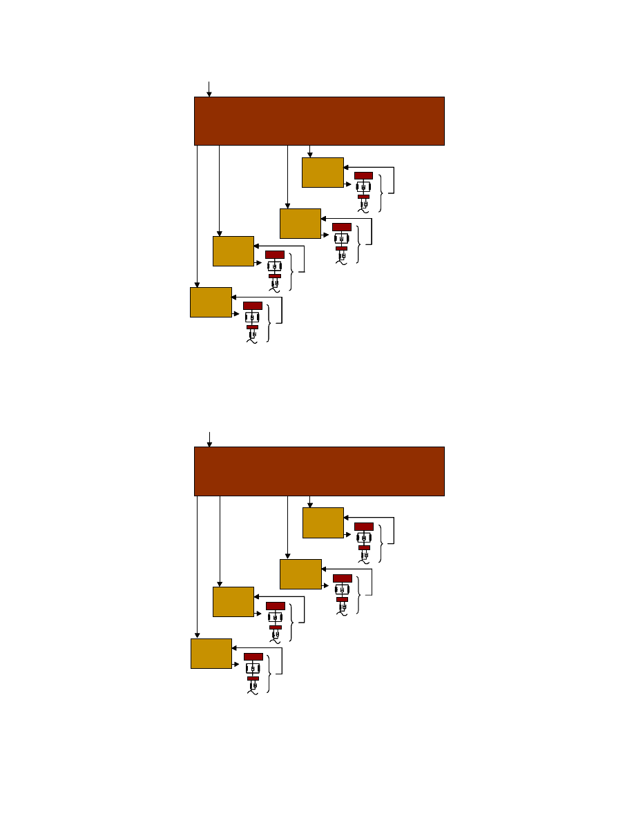
1.1.1

Low Level Control

Figure 1.1 depicts the simplest controller on the HMMWV, PI position control. This is

needed to stabilize the system once the actuators are powered. There are 4 independent

controllers, one for each wheel. For coordinated motion there is a central, desired

position generator.

2

LHR

PID

RHR

PID

RideHeight Generator

LHF

PID

RHF

PID

Desired Motion

{pos}

{d

e

s pos

it

io

n}

{spl cmd}

LHR

PID

LHR

PID

RHR

PID

RHR

PID

RideHeight Generator

LHF

PID

LHF

PID

RHF

PID

RHF

PID

Desired Motion

{pos}

{d

e

s pos

it

io

n}

{spl cmd}

Figure 1.1: Diagram of PI control structure, 4 sensors required

Replacing the PI controllers with Force Tracking Controllers (FTC’s) one obtains the

FTC validation mode. Note that more sensors are needed but the structure is the same.

LHR

FTC

RHR

FTC

Force Generator

LHF

FTC

RHF

FTC

Desired Motion

{pos, frc, spl volt}

{d

e

s f

o

rce

}

{spl cmd}

LHR

FTC

LHR

FTC

RHR

FTC

RHR

FTC

Force Generator

LHF

FTC

LHF

FTC

RHF

FTC

RHF

FTC

Desired Motion

{pos, frc, spl volt}

{d

e

s f

o

rce

}

{spl cmd}

Figure 1.2: Diagram of FTC structure, 12 sensors required

3

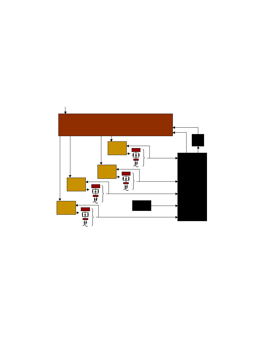
1.1.2

Control without Preview

When running just the lower level controllers, a profile generator is used to create the

desired trajectories. To make the system responsive, a high-level control algorithm

replaces this profile generator. In general these schemes require information about the

full car vehicle states. Or if not, using full sensor information and a Kalman filter

enhances the information they do use.

Kalman

Filter

HRF

MPC – SkyHook – LQR – VDC*

Performance Criteria

{pos, frc, spl volt}

{cha accel,
p&r rates}

{pos, frc,
hub accel}

{abs power}
{14 states}

{d

e

s f

o

rc

e

}

* VDC uses a controller other than FTC

{spl cmd}

Chassis
Sensors

LHR

FTC

RHR

FTC

LHF

FTC

RHF

FTC

Kalman

Filter

HRF

MPC – SkyHook – LQR – VDC*

Performance Criteria

{pos, frc, spl volt}

{cha accel,
p&r rates}

{pos, frc,
hub accel}

{abs power}
{14 states}

{d

e

s f

o

rc

e

}

* VDC uses a controller other than FTC

{spl cmd}

Chassis
Sensors

LHR

FTC

LHR

FTC

RHR

FTC

RHR

FTC

LHF

FTC

LHF

FTC

RHF

FTC

RHF

FTC

Figure 1.3: Diagram of higher level control structure, 20 sensors required

The Velocity Damping Controller (VDC) scheme offered in Figure 1.3 will not be

discussed any further. It is provided here as an alternative to the force based control

paradigms. VDC attempts to dampen chassis motion by converting axle acceleration to a

desired suspension velocity. A low-level controller comparable to the FTC, described in

Chapter 2, is necessary to implement the VDC.

4

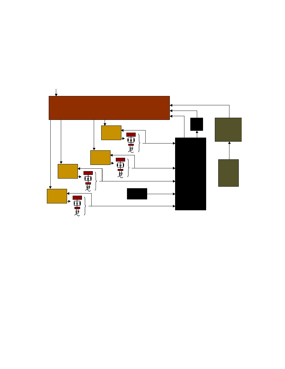
1.1.3 Preview

Control

With the controllers of the previous sections well tuned, the preview information is

added. The sensor data must be corrected for vehicle motion at the time of measurement

and buffered until the higher-level controllers need it. More detail on these subsystems is

provided in Chapter 3.

Kalman

Filter

HRF

Preview

Sensors

HPR

Correction

& Buffer

Chassis
Sensors

LHR

FTC

RHR

FTC

MPC

p

- FSLQ

p

LHF

FTC

RHF

FTC

Performance Criteria

{pos, frc, spl volt}

{cha accel,
p&r rates}

{pos, frc,
hub accel}

{abs power}
{14 states}

{preview}

{d

e

s f

o

rc

e

}

{spl cmd}

Kalman

Filter

HRF

Preview

Sensors

HPR

Correction

& Buffer

Chassis
Sensors

LHR

FTC

LHR

FTC

RHR

FTC

RHR

FTC

MPC

p

- FSLQ

p

LHF

FTC

LHF

FTC

RHF

FTC

RHF

FTC

Performance Criteria

{pos, frc, spl volt}

{cha accel,
p&r rates}

{pos, frc,
hub accel}

{abs power}
{14 states}

{preview}

{d

e

s f

o

rc

e

}

{spl cmd}

Figure 1.4: Diagram of preview control structure, 22 sensors required

The Frequency Shaped Linear Quadratic (FSLQ) Controller is a Linear Quadratic

Regulator (LQR) mathematically formulated in the presence of a frequency shaping

Human Response Filter (HRF), see Sections 4.3 & 3.4 respectively. An FSLQ

p

Controller can be designed to use the available preview information [20]. FSLQ

p

simulations were carried out by SSCI for realistic road profiles provided by TARDEC.

Performance was comparable with the MPC

p

but FSLQ

p

control does not explicitly

handle system constraints and will not be considered further.

5

1.2 HMMWV Equipment

Lotus Engineering, England, completed original instrumentation of the HMMWV. The

University of California at Berkeley added additional sensors and a new computer, see

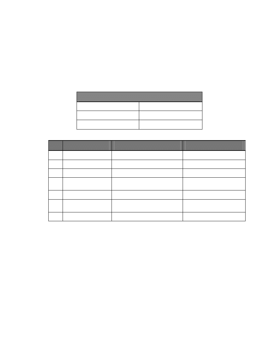
Appendix A. Provided below are tables detailing the important information regarding the

sensor and actuator suites.

Vickers PV3-115 Hydraulic Pump

Supply Pressure

3000 psi

Flow Rate

45 liters/min

Power Consumption

< 32 hp @ < 3500 rpm

Table 1.1: Important hydraulic pump specifications

Qty

Sensor Type

Location

Measurement

4

Load Cell

Top mount of each actuator

Actuator forces

4

LVDT

Inside each actuator

Actuator displacement

4

Hub Accelerometer On each wheel hub

Axle vertical acceleration

2

Chassis
Accelerometer

Opposite corners of chassis

Chassis vertical
acceleration

2

Rate Gyro

Center console

Pitch and Roll rates

2

Range

Front of vehicle

Preview, distance to
ground

1

Speedometer

Engine compartment

Vehicle speed

Table 1.2: Essential HMMWV sensors

The processor suite of choice is the dSpace Autobox components described below. More

information on the processors and configurations is provided in Appendix B.

Digital Signal Processing Boards:

DS1003: TI TMS320C40 Parallel 60MHz DSP board

DS1004: DEC Alpha AXP21164 300MHz DSP board

6

Chapter 2 - FTC Design

2.1 Overview of Controller

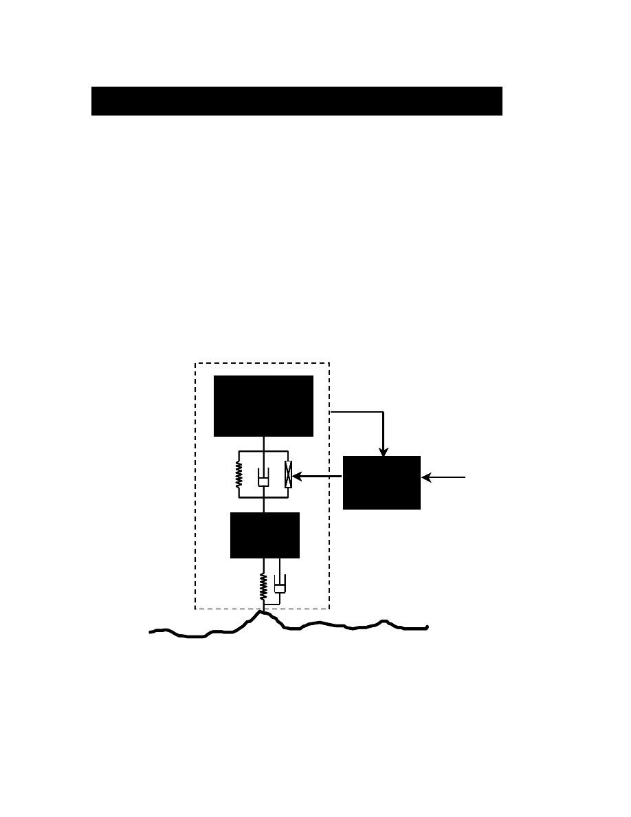
The force-tracking controller regulates the force of an individual actuator to the desired

force prescribed by a higher-level controller. Although the higher-level controller may

make decisions based upon the full car model, it is sufficient to only consider the quarter

car dynamics when designing a controller for a single actuator. For the actual system, the

added dynamics due to full car motion may be considered as model errors. A method to

compensate for these model errors is presented at the end of the controller formulation.

Force

Control

Fdes

udes

1/4 Vehicle

measurements (1 msec)

Sprung

Mass

Unsprung

Mass

kt

bt

ks bs

F

Force

Control

Force

Control

Fdes

udes

1/4 Vehicle

measurements (1 msec)

Sprung

Mass

Unsprung

Mass

kt

bt

ks bs

F

Sprung

Mass

Sprung

Mass

Unsprung

Mass

Unsprung

Mass

kt

bt

kt

bt

ks bs

F

ks bs

F

Figure 2.1: Diagram of force tracking controller system

7

2.2 Plant Models

2.2.1 Quarter

car

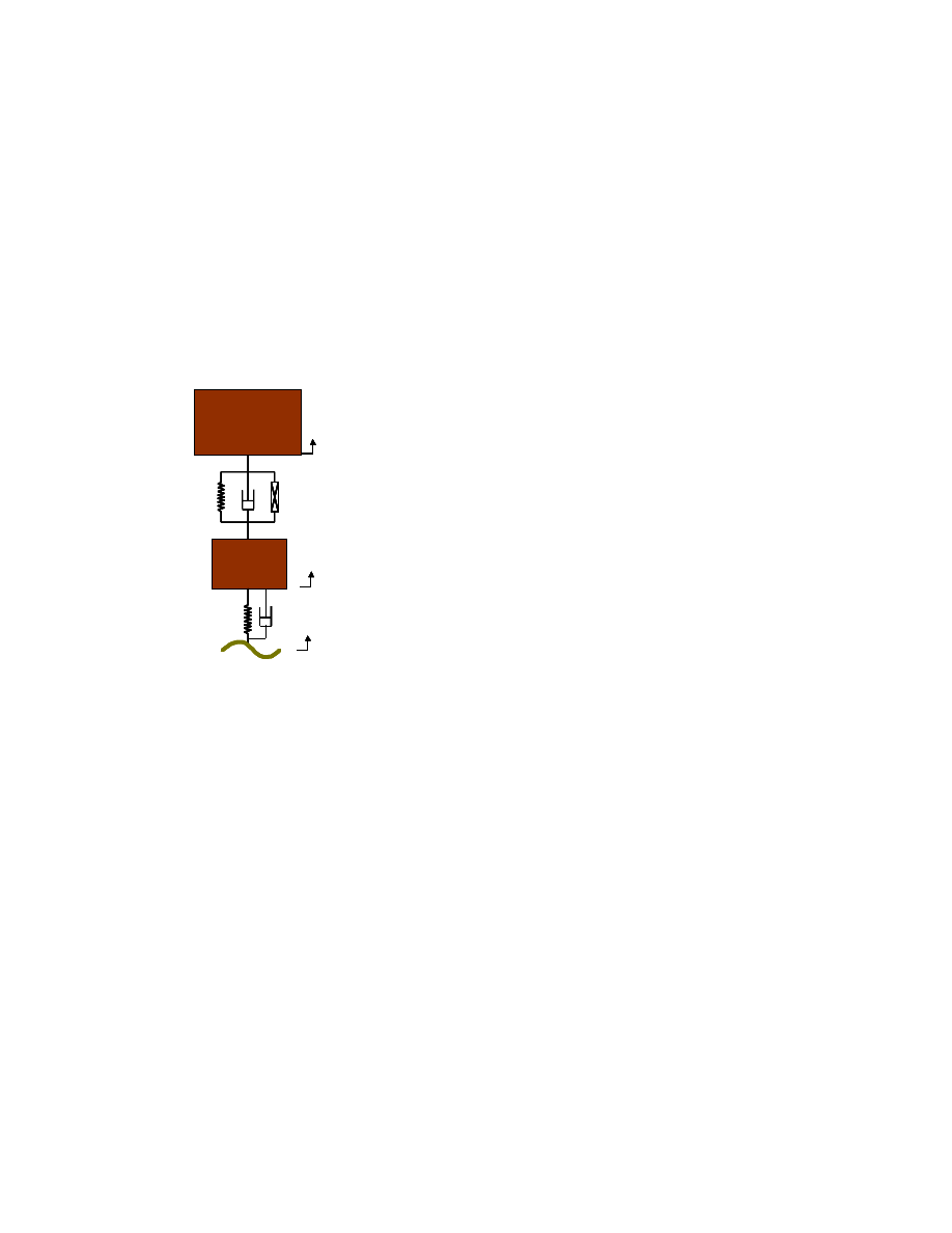
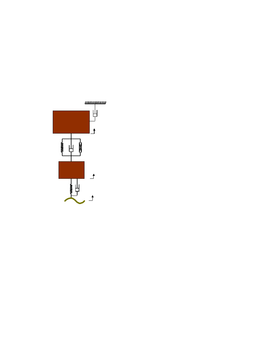
A standard quarter car model was used, see Figure 2.2 for schematic and dynamic

equations. One item to note is the existence of a pure damping element in parallel with

the hydraulic actuator. In a typical application the shock is removed. However, the

simulation behaves closer to the actual system when a pure damping element with a low

damping coefficient is used.

s

s

f

a

s

u

s

s

u

s

ms

x

m

F

F

x

x

k

x

x

c

F

&&

&

&

=

−

+

−

+

−

=

∑

)

(

)

(

s

s

x

x &,

u

u

x

x &,

r

r &,

Sprung

Mass

Unsprung

Mass

kt

bt

ks bs

F

s

s

x

x &,

u

u

x

x &,

r

r &,

s

s

x

x &,

s

s

x

x &,

u

u

x

x &,

u

u

x

x &,

r

r &,r

r &,

Sprung

Mass

Unsprung

Mass

kt

bt

ks bs

F

Sprung

Mass

Unsprung

Mass

kt

bt

ks bs

F

Sprung

Mass

Sprung

Mass

Unsprung

Mass

Unsprung

Mass

kt

bt

kt

bt

ks bs

F

ks bs

F

u

u

f

a

u

s

s

u

s

s

u

t

u

t

mu

x

m

F

F

x

x

c

x

x

k

x

r

k

x

r

c

F

&&

&

&

&

&

=

+

−

−

+

−

+

−

+

−

=

∑

)

(

)

(

)

(

)

(

Figure 2.2: Diagram and equations for the quarter car model

It is convenient to define the state vector as follows when writing these equations in state

space:

]

,

,

,

[

s

s

u

u

u

x

x

x

x

x

r

&

&

−

−

=

β

(2.1)

2.2.2 Hydraulic

actuator

The hydraulic actuators are governed by electro hydraulic servovalves and are mounted

in parallel to the passive suspension springs, allowing for the generation of forces

between the sprung and unsprung masses.

The electro hydraulic system consists of an actuator, a primary power spool valve and a

secondary bypass valve. As seen in Figure 2.3, the hydraulic actuator cylinder lies in a

follower configuration to a critically centered electro hydraulic power spool valve with

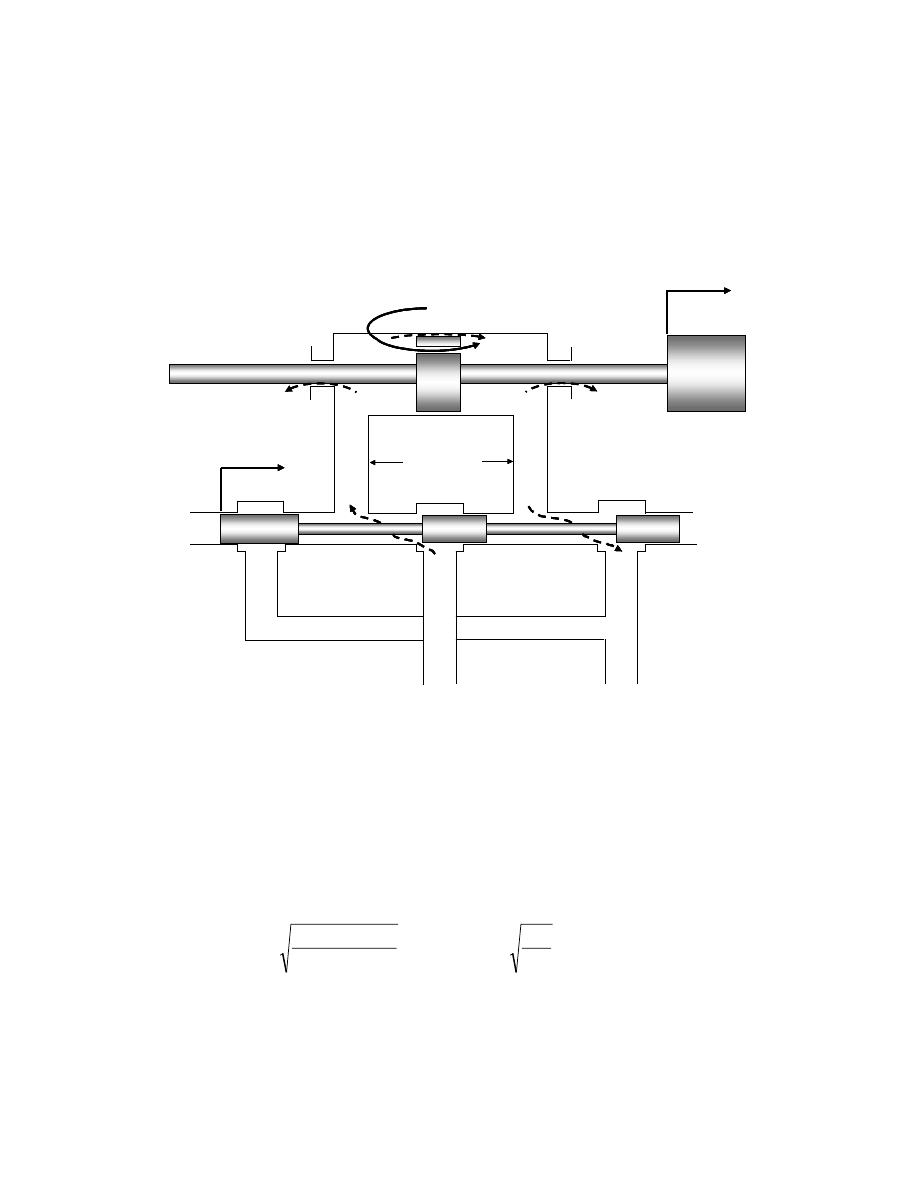
8

matched and symmetric orifices. Positioning of the spool u

1

directs high pressure fluid

flow to either one of the cylinder chambers and connects the other chamber to the pump

reservoir. This flow creates a pressure difference P

L

across the piston. This pressure

difference multiplied by the piston area A

p

is what provides the active force F

A

for the

suspension system.

Spool

Piston

P

1

Q

1

P

L

= P

1

- P

2

Supply

Return

P

S

P

R

Q

2

P

2

V

1

V

2

C

em

P

1

C

em

P

2

C

im

P

L

F

A

u

1

u

2

A

p

Spool

Spool

Piston

P

1

Q

1

P

L

= P

1

- P

2

Supply

Return

P

S

P

R

Q

2

P

2

V

1

V

2

C

em

P

1

C

em

P

2

C

im

P

L

F

A

u

1

u

2

A

p

Figure 2.3: Physical schematic and variables for the hydraulic actuator.

Dynamics for the hydraulic actuator [15] valve are given below. Parameter definitions

and experimental values are given in the Glossary. The change in force is proportional to

the position of the spool with respect to center, the relative velocity of the piston, and the

leakage through the piston seals. A second input u

2

may be used to bypass the piston

component by connecting the piston chambers.

)]

(

2

)

sgn(

)

sgn(

[

2

2

1

1

1

u

s

p

L

tm

L

L

d

L

S

d

p

A

x

x

A

P

C

P

P

u

C

P

u

P

wu

C

A

F

&

&

&

−

−

−

−

−

=

ρ

ρ

α

(2.2)

The bypass valve u

2

could be used to reduce the energy consumed by the system. If the

spool position u

1

is set to zero, the bypass valve and actuator will behave similar to a

9

variable orifice damper. For the purposes of proving the viability of the FTC the bypass

valve input u

2

is set to zero during experiments.

Spool valve positions u

1

and u

2

are controlled by a current-position feedback loop. The

essential dynamics of the spool have been shown to resemble a first order system forced

by a voltage for frequencies less than 15 Hz [7].

kv

u

u

=

+

&

τ

(2.3)

2.2.3 Complete

system

The system to be controlled by the FTC is the combined quarter car plant and hydraulic

actuator; spool voltage is the control input. Defining the state x

5

= P

L

= F

A

/A

p

and

choosing the state vector (2.4) the state space representation of the system can be written

as in Figure 2.4. Suspension friction and road disturbance are considered model errors

and are not shown here.

]

,

,

,

,

,

[

1

u

A

F

x

x

x

x

x

r

X

p

A

s

s

u

u

u

&

&

−

−

=

(2.4)

V

k

X

C

A

A

m

A

m

c

m

k

m

c

m

A

m

c

m

k

m

c

c

m

k

X

tm

p

p

s

p

s

s

s

s

s

s

u

p

u

s

u

s

u

s

t

u

t

































































+





































































Φ

+





































































−

−

−

−

−

−

−

+

−

−

=

τ

τ

α

α

α

0

0

0

0

0

0

0

0

0

0

1

0

0

0

0

0

0

0

0

0

0

0

0

1

0

1

0

0

0

0

0

0

1

0

&

ρ

α

5

6

6

)

sgn(

x

x

P

wx

C

where,

s

d

−

=

Φ

Figure 2.4: FTC plant dynamics in state space form

10

2.3 Control Algorithms

As seen in Figure 2.4 there is a severe non-linearity

Φ

in the dynamic behavior of the

system. The most direct approach to solving this problem is dynamic surface control [3].

However, as will be developed, this method results in some undesirable internal

dynamics. The concept of Output Redefinition (ORD) is one solution to this problem.

Using ORD makes it possible to adaptively determine the value of the suspension

damping, c

s

, in Figure 2.2 [14]. Simulation and implementation issues are addressed as

well.

2.3.1

Dynamic Surface Control

In general, dynamic surface control reduces an n

th

order system to n 1

st

order systems.

The output is differentiated with respect to time. Controllers are chosen to regulate a

synthetic control input for each differentiation step. Progressive synthetic input choices

should be one derivative closer to the real system input. If the input appears after m<n

steps then there are n-m internal dynamic states. A controller is designed for each of the

m 1

st

order systems. Since there are no controllers for the internal dynamics, it is

essential that the internal dynamics be well behaved. Dynamic surface control typically

utilizes a sliding surface controller for each of the m 1

st

order surfaces. If necessary,

input-output linearization could be applied to system prior to the dynamic surface control

method. Input-output linearization often results in the undesirable differentiation of

model errors. For more information on dynamic surface control consult reference [17].

For the system in Figure 2.4, the control enters through the spool voltage. Appling the

method described above, the resulting system has relative degree 2 and thus 4 internal

dynamics states. In this case, the internal dynamics are precisely those of the quarter car

suspension system. These dynamics are marginally stable and thus highly oscillatory due

to the lack of a pure, physical damping element. Since there exists a direct feedback path

from suspension velocity to hydraulic actuator force, Equation (2.2), the suspension

oscillations could result in undesirable force tracking performance [4].

11

Derivation of Control Law

The output F

A

was differentiated with respect to time until the control input appeared.

The resulting controller surfaces are

spool

p

u

&

A

A

L

F

P

=

(2.5)

For the P

L

surface, an integral term was added to the standard definition of s. The

integral term, weighted by 0 <

λ

1

< 1, slightly attenuates control noise.

d

5

x

x

x

where

dt

x

x

s

5

5

5

1

5

1

~

~

~

−

=

+

=

∫

λ

(2.6)

Applying the sliding surface approach, the control law must satisfy the condition in

Equation (2.7) to ensure asymptotic tracking of F

des

.

(

)

2

1

1

5

1

5

1

1

1

~

~

s

x

x

s

s

s

η

λ

−

≤

+

=

&

&

(2.7)

Plugging in the equation of dynamics for

d

x

5

&

and solving for u

des

:

(

)

{

}

1

1

5

1

5

5

2

4

~

1

s

x

x

x

C

x

x

A

u

d

tm

p

des

η

λ

α

α

−

−

+

+

−

Φ

=

&

(2.8)

In Equation (2.8) the desired force profile enters through the terms

d

x

5

&

and s

1

. Because

the time derivative of the desired force is used in control computation, it is important for

the force profile to be smooth.

Following the method used for the P

L

surface, the equation for control input V can be

obtained as follows:

(

)

2

2

2

2

2

2

2

s

u

u

s

s

s

u

u

s

des

des

η

−

≤

−

=

−

=

&

&

&

(2.9)

Substituting the equation of dynamics for

u&

into Equation (2.9) and solving, the control

input is thus:

{

}

2

2

1

s

u

u

k

V

des

τ

η

τ

−

+

=

&

(2.10)

The time derivative of u

des

is needed to compute the control input V. Using the filter of

Equation (2.11) allows theoretical proof that the resulting controller is asymptotically

stable.

12

τ

ψ

ψ

−

=

des

u

&

(2.11)

ψ

&

is used in place of

des

u

&

in Equation (2.10). The state

ψ

is maintained via forward

Euler integration of

ψ

&

.

In theory, the sliding surface gains

i

η

are chosen to overcome the worst-case model and

disturbance errors. In practice, the control input is limited by system capabilities; see

Section 2.5 for more details.

2.3.2 Output

Redefinition

Dynamic surface control ensures asymptotic tracking of the desired profile provided the

sliding surface gains,

η

i

, can be made sufficiently high as to overpower any errors.

Output redefinition reduces model errors by directly considering the lack of a pure

damping element in the system. The output is modified such that an artificial damping

term is added to the system. As per Osorio et al [14] the modified output can be written

as

[

]

v

v

A

s

u

v

A

m

k

k

K

and

F

y

where

K

y

x

x

k

F

y

−

=

=

−

=

−

−

=

0

0

)

(

β

&

&

(2.12)

New synthetic inputs are developed for the modified system by using suspension

measurements. New desired outputs are obtained by using the quarter car model to

compute the expected suspension terms. The gain k

v

is chosen such that the state

feedback matrix (PK+Q), in Equation (2.14), is Hurwitz. The general procedure for

developing the control law using the modified output is explained below, more detail is

given in the reference sited above. For instance, Osorio et al [14] proves that if a

controller is designed to asymptotically track the modified output then the original output

is also obtained.

Controller derivation begins by writing the internal dynamic equations in matrix form,

using the vector

β

from Equation (2.1), the upper 4x4 matrix Q from Figure 2.4, and

[

]

T

1

0

1

0

s

u

m

m

P

−

=

to obtain:

13

β

Q

Py

β

+

=

&

(2.13)

From Equation (2.12) and Equation (2.13) it follows that

β

β

β

)

(

Q

PK

Py

K

F

y

m

A

m

+

+

=

−

=

&

&

&

&

(2.14)

Now, deriving the sliding approach for the y

m

surface:

des

m

m

y

y

s

−

=

1

1

1

1

)

)

(

(

s

y

Q

PK

Py

K

F

s

des

m

m

A

η

β

−

=

−

+

+

−

=

&

&

&

(2.15)

Substituting the valve dynamics of Equation (2.2) into Equation (2.15), the control law is

found to be

(

)

[

]

{

}

1

1

2

4

)

(

1

s

y

Q

PK

Py

K

F

C

x

x

A

u

des

m

m

A

tm

p

des

η

β

α

α

−

+

+

+

+

+

−

Φ

=

&

(2.16)

The sliding surface controller developed above provides a method to compensate for the

lack of a pure, physical damping element in the system. This surface is a modified form

of the P

L

=F

A

/A

p

surface of the original FTC formulation, Equation (2.8).

2.3.3 Parameter

Adaptation

Several times throughout this derivation the need for a pure damping element in the

suspension models and controllers has been mentioned. Since there is no physical

damper it is difficult to estimate what the proper amount of damping should be; here, an

adaptive algorithm is derived for this purpose. The methodology can also be used to

estimate other system parameters, provided the parameters are estimated individually.

Derivation of Update Law

The parameter c

s

appears in the redefined output dynamic Equation (2.12) not in the

original output P

L

. Thus, the redefined output will be used. Dynamics written in terms

of c

s

are

{ }

(

)

)

(

...

4

2

x

x

m

c

k

F

y

eq

s

v

A

m

−

−

+

=

s

s

c

c

where

∆

+

=

ˆ

c

s

(2.17)

Using the sliding surface as described in Equation (2.15) and the Lyapunov like function:

14

2

2

2

2

1

s

c

s

∆

+

=

ρ

l

(2.18)

Differentiating Equation (2.18), substituting

s&

from Equation (2.15), and using the

control law (2.16) we obtain (2.19). The system uses c

s

, the controller uses

s

cˆ , and

0

=

s

c

&

.

(

)

s

eq

s

c

s

m

x

x

c

s

&

l&

ˆ

)

(

1

4

2

2

1

1

ρ

η

−

−

∆

+

−

=

(2.19)

To ensure that Equation (2.19) is negative semi-definite we must cancel the second term.

Thus the parameter update law is

2

1

1

4

2

)

(

ˆ

s

s

m

x

x

c

eq

s

η

ρ

−

=

⇒

−

=

l&

&

(2.20)

Since the estimate of c

s

is time varying and the Lyapunov function time derivative is only

negative semi-definite, Barbalat’s lemma must be applied:

bounded

is

s

s

2

-

b/c

continous

uniformly

is

definite

-

semi

negative

is

zero

by

bounded

lower

is

&

l&&

l&

l&

l

σ

=

•

•

•

(2.21)

Thus, the parameter c

s

may be adaptively determined. Unfortunately, sliding surface s

1

does not converge in simulation or in implementation. Thus, the parameter c

s

does not

converge either.

2.4 Simulation

Before implementing the controller on the HMMWV the control code was tested via

Simulink simulation.

2.4.1 Setup

Below is an image of one Simulink model used to simulate controller performance. The

plant dynamics of the quarter car and hydraulic valve are simulated given an erroneous

set of parameters. Road input and suspension friction disturbances are also added to the

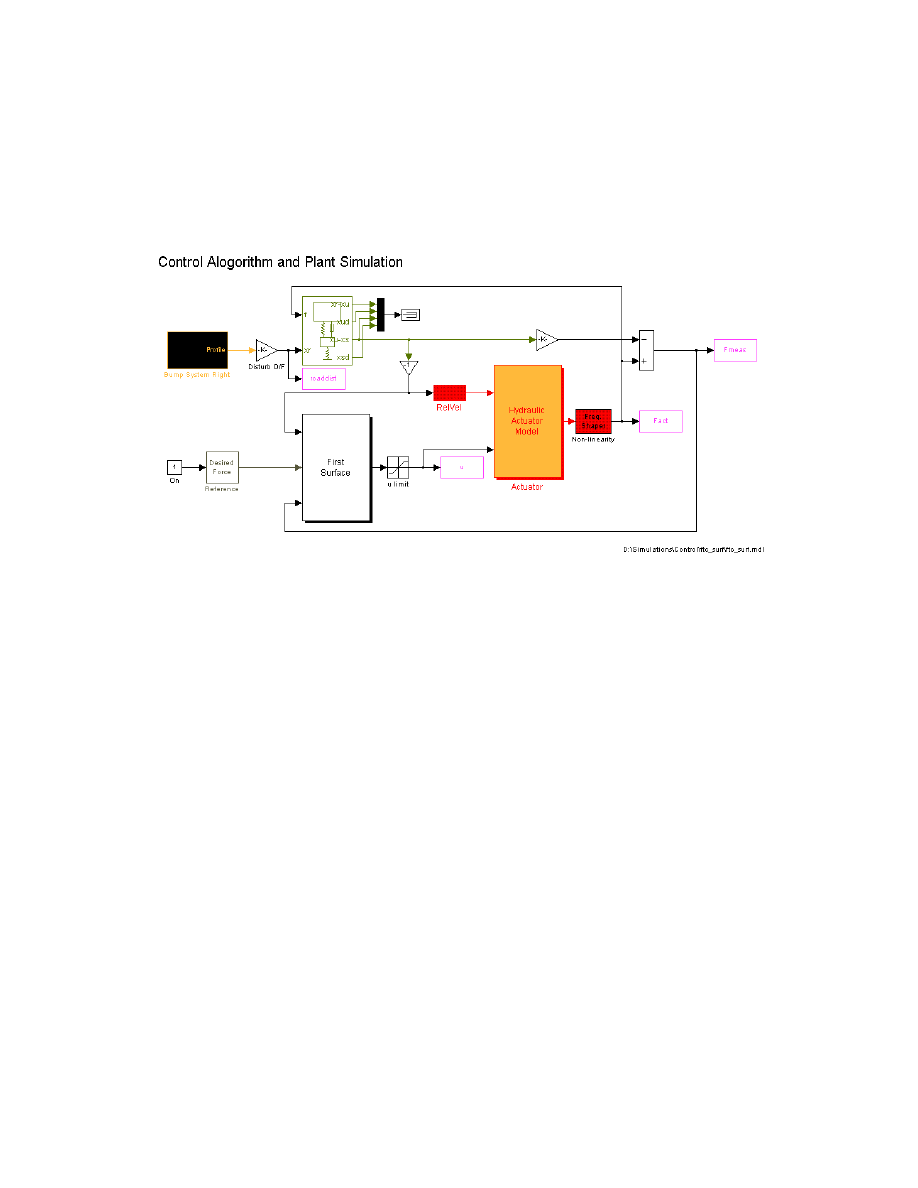
15

plant. The controller used the correct, fixed set of parameters, and the only allowable

modification to the control algorithm was an increase in the sliding surface gains,

η

i

.

Spool voltage is limited to

±

10 Volts. Sliding surface gains should not be increased as to

cause control input saturation.

Figure 2.5: Simulink FTC simulation setup, quarter car plant

2.4.2

Model Error Approximation

Without the existence of significant model error the controller simulation would, and did,

result in perfect tracking. Experimental data depicted considerable model error in the

range of 1Hz to 5Hz. The most likely cause of this is the un-modeled, full car resonant-

mode, dynamic feedback from the suspension relative velocity to the actuator chamber

pressure. To compensate for this, a model error filter was created, the “Freq. Shaper”

block in Figure 2.5. System output was attenuated at 1Hz and amplified at 5Hz by two,

second order filters in series. For dynamic surface control it is required that the error be

additive to a nominal plant. If the phase error is neglected then the filter error is in that

form and the controller is still theoretically viable.

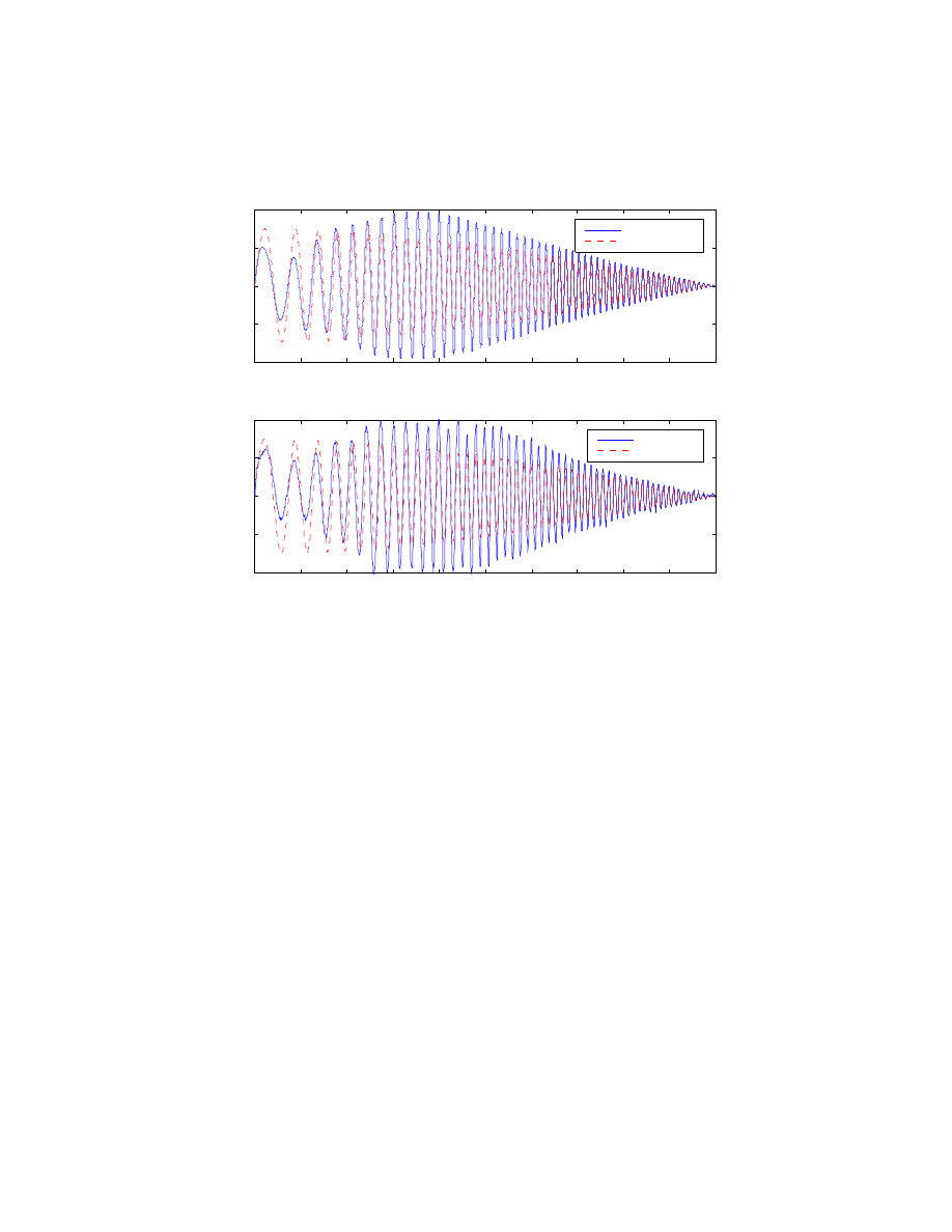
The same controller, gains, and parameters were used both in simulation and on the

physical system. The plot below depicts comparable error dynamics; the dotted line is

16

the desired trajectory. With the model error filter, simulation results are more accurate

representations of what the HMMWV will do given a specific controller.

0

1

2

3

4

5

6

7

8

9

10

−1000

−500

0

500

1000

Force (N)

Simulated & Experimental Force Tracking Control Output

Simulated

Desired

0

1

2

3

4

5

6

7

8

9

10

−1000

−500

0

500

1000

Force (N)

Time (sec)

Actual

Desired

Figure 2.6: Plot of simulated (top) vs. actual (bottom) controller performance

2.4.3 Simulation

Results

Simulation of the control algorithm proved useful in debugging the code and also spurred

the development of a new, empirical control scheme. By creating the model error

approximation filter to make the simulation look like the actual system performance, it

was realized that the inverse filter could be used to improve tracking near the resonant

modes of the suspension, see Section 2.5.2.

2.5 Implementation

Tuning the FTC was an arduous process, exacerbated by the lack of accurate system

parameter information. Parameter information was not well documented and it was very

17

difficult to conduct parameter validation tests. That aside, the following modifications to

the theory proved useful.

2.5.1 Noise

Filters

The desired spool position command output by the first surface, P

L

, was very noisy. The

second surface amplified the noise and coincidently decreased sliding mode gains. It was

empirically determined that the filter in Equation (2.22) reduced control noise and

improved controller performance. With this filter, u'

des

replaced the u

des

command sent to

the second surface in Equation (2.9).

2

)

2

(

)

1

(

'

−

+

−

=

k

u

k

u

u

des

des

des

(2.22)

Another empirical study showed that numerical differentiation, Equation (2.23), of

des

u

&

worked better than the sliding mode filter described in Equation (2.11).

t

k

w

k

w

k

w

des

des

des

∆

−

−

=

)

1

(

)

(

)

(

&

(2.23)

2.5.2

Model Error Filters

The FTC formulation above treats the full car dynamics as a disturbance. Results

indicated that FTC performance around the resonant modes for chassis motion was poor.

Resonant frequency for the pitch and heave modes is around 2Hz and around 4Hz for the

roll mode. Filtering the u

des

command by a filter that attenuates inputs around these

frequencies improved force tracking. To implement these filters with high-level

controller force generation, a heave, pitch, and roll quantification scheme was used.

Ultimately, FTC tuning was improved to eliminate the need for these filters. Moreover,

MPC formulation considers these resonant frequencies when computing F

des

.

2.5.3

High-Level Control Filters

The hierarchical control inputs were generated at a 30ms sampling rate while the FTC ran

at 1ms. A 1ms sampling rate was necessary to ensure good tracking up to 8Hz as dictated

by the system time constants. For smooth convergence to F

des

, considering the derivative

18

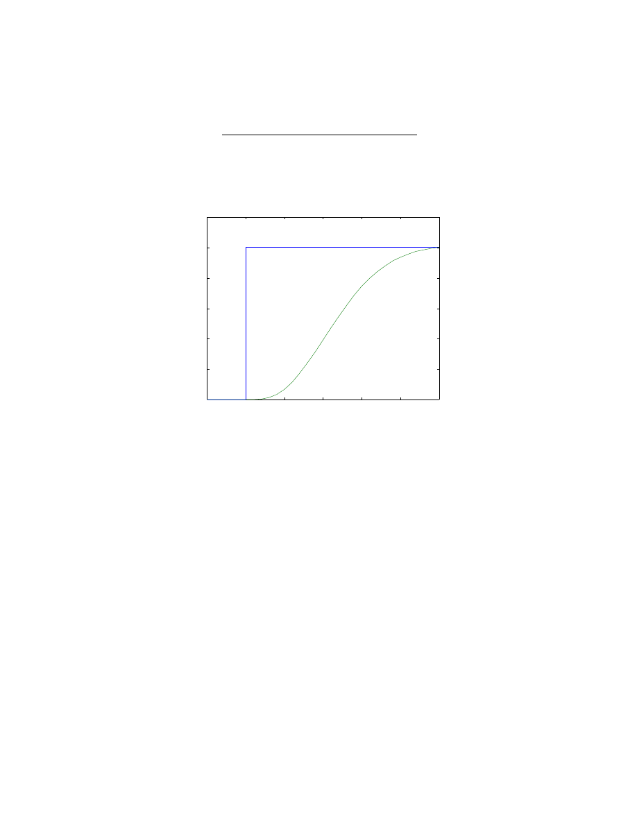
terms in Equation (2.8), the desired force was filtered by Equation (2.24), the rise time is

approximately 27ms.

9

4

.

6

7

6

.

7

385625

950

9

4

.

6

)

(

Fˆ

2

3

4

des

e

s

e

s

s

s

e

s

+

+

+

+

=

(2.24)

A plot of the filter step response is shown below for better understanding of filter

functionality.

0

0.005

0.01

0.015

0.02

0.025

0.03

0

200

400

600

800

1000

1200

Force (n)

Time (sec)

Step Response of Smoothing Filter

Figure 2.7: Plot of F

des

smoothing filter step response

19

Chapter 3 - Subsystems

Most of these systems are presented in other project reports; they are summarized here to

provide a more complete understanding of the system. However, components that

contain unique, personal, contributions are discussed in more detail. All of the systems

are necessary for the successful implementation of the MPC

p

controller.

3.1 Safety Systems

Emergency Shut Down

Two independent switches can affect a shutdown. One switch, near the driver, is a

software shutdown; it opens actuator bypass valves and damps the control output to zero

smoothly. The other toggle switch, by the passenger, is a hard shutdown; it is directly

wired to open the hydraulic pump bypass. With the bypass open no power is supplied to

the actuators. Typically, the first shutdown is sufficient to handle occasional controller

instabilities.

Signal Checking

This safety check alerts the driver that a sensor is disconnected. A bit of logic checks for

the existence of sensor noise on the respective input channel. No noise implies the sensor

is disconneceted.

3.2 Preview Information

The MPC

p

requires the road profile, Z

road

, and the rate that Z

road

is changing with respect

to time

road

Z&

for n preview steps, or preview horizon (pH), at each wheel. Road profiles

for each side of the car are stored in a buffer. When extracting preview data the buffer is

parsed and information of the current vehicle velocity and Z

road

are combined to create

road

Z&

. The HMMWV system has two methods to obtain Z

road

.

20

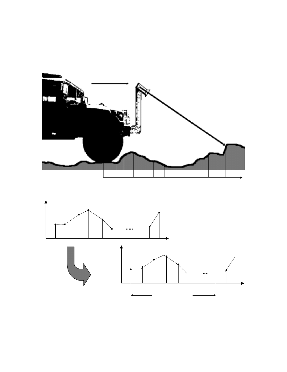
3.2.1 Preview

Generation

Preview generation can be used on courses with a known road profile, such as the test

track, see Appendix D. The preview buffer is fed a pre-stored profile in place of the

sensor preview data. The digital profile is synchronized to the actual profile using

standard HMMWV sensors. Below is a sample buffer output matched with peaks from

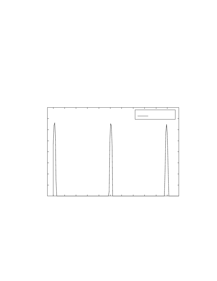
the suspension load cells. The trigger spikes indicate the most probable location of the

actual bump. This method relies on absolute position and is therefore susceptible to error

accumulation. At 10m the real bump is almost beyond the buffered preview generation

predicted location. To contrast, buffered sensor data requires only slightly more than the

length of the vehicle, at most 4m.

0

1

2

3

4

5

6

7

8

9

10

11

0

0.01

0.02

0.03

0.04

0.05

0.06

0.07

0.08

Dis tanc e Traveled [m ]

P

rof

il

e [

m

]

Trigger
B uffer Output

Figure 3.1: Plot of generated & buffered preview data matched with load cell peaks

3.2.2

Preview Sensor Correction

While preview generation makes debugging a bit easier, it is not useful in the proposed

application. For that we use preview sensors that measure the range to ground. Sensors

measurements must be converted to a road height. In practice the preview sensor mount,

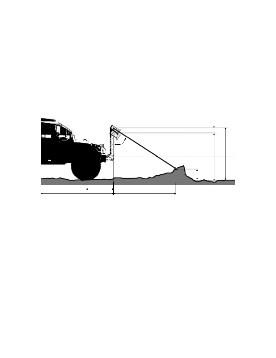
21

rigidly attached to the chassis, see Appendix A, will have some heave, pitch and roll

(HPR). Assuming that the assembly is a rigid body with negligible warp, it is possible to

compensate for chassis motion by trigonometric relations. HPR are measured much

faster than the rate of change of HPR. Thus, it is reasonable to apply trigonometry

directly to the measurements, obtaining the following equations:

f

meas

road

bias

lat

long

sens

meas

sens

road

X

D

X

D

CG

CG

H

Z

D

Z

Z

+

−

=

+

−

−

=

−

−

=

)

sin(

cos

sin

sin

)

cos(

θ

α

α

φ

θ

θ

α

(3.1)

Where the variables are defined as

h

bias

D

meas

H

Z

road

Z

sens

αααα

CG

long

X

f

Θ =

Θ =

Θ =

Θ =

Pitch

Φ =

Φ =

Φ =

Φ =

Roll

X

road

h

bias

D

meas

H

Z

road

Z

sens

αααααααα

CG

long

X

f

Θ =

Θ =

Θ =

Θ =

Pitch

Φ =

Φ =

Φ =

Φ =

Roll

X

road

Figure 3.2: Diagram and nomenclature definition for preview correction

The set of values X

road

and Z

road

are now be fed to the buffer and used to attain proper

preview information for the MPC

p

.

Equations (3.1) rely on accurate HPR measurements to ascertain correct road

information. To be accurate, the HPR computation must also include the road profile

under the wheels. Experiments have shown that the problem is more complicated than

simply accounting for the road height under the wheel. Further discussion of this topic is

presented in Section 3.2.4.

3.2.3 Preview

Buffer

Incoming road information is sorted, stored, and updated by the buffer with respect to

X

road

. Interpolated data is retrieved for the requested pH for each wheel.

22

Consecutive road data is not guaranteed to have an equal spacing or even a consistent

order. Graphically, the input to the buffer and buffer processing are depicted in Figure

3.3 & Figure 3.4.

current
sample

vehicle speed

V

k

Z

k+n

Z

k

Z

k+1

Z

k+2

Z

k+3

Z

k+4

Z

k+5

Z

k+n-1

distance

current
sample

vehicle speed

V

k

Z

k+n

Z

k

Z

k+1

Z

k+2

Z

k+3

Z

k+4

Z

k+5

Z

k+n-1

distance

Figure 3.3: Diagram of unevenly spaced road height samples

road profile

height

distance

Z

k+n

Z

k

Z

k+1

Z

k+2

Z

k+3

Z

k+4

Z

k+5

Z

k+n-1

road profile

height

Z

j

Z

j+1

Z

j+2

Z

j+3

Z

j+4

Z

j+m

T

T

T

T

T

total preview time

V

k

road profile

height

distance

Z

k+n

Z

k

Z

k+1

Z

k+2

Z

k+3

Z

k+4

Z

k+5

Z

k+n-1

road profile

height

distance

Z

k+n

Z

k

Z

k+1

Z

k+2

Z

k+3

Z

k+4

Z

k+5

Z

k+n-1

road profile

height

Z

j

Z

j+1

Z

j+2

Z

j+3

Z

j+4

Z

j+m

T

T

T

T

T

total preview time

road profile

height

Z

j

Z

j+1

Z

j+2

Z

j+3

Z

j+4

Z

j+m

T

T

T

T

T

total preview time

V

k

V

k

Figure 3.4: Interpolation and re-sampling of the road profile preview information

23

A standard velocity sensor is used to measure V

k

for the experimental HMMWV. In final

implementation, an accurate estimation of the ground speed is required to avoid errors

introduced by wheel slip, by wheel liftoff, and by loss of traction.

The buffer is fixed length, circulating memory. An integer increment in the array pointer

corresponds to a fixed increment in the physical distance. To improve the stochastic

properties of the buffer, new information is interpolated and updated, if necessary, with a

forgetting factor.

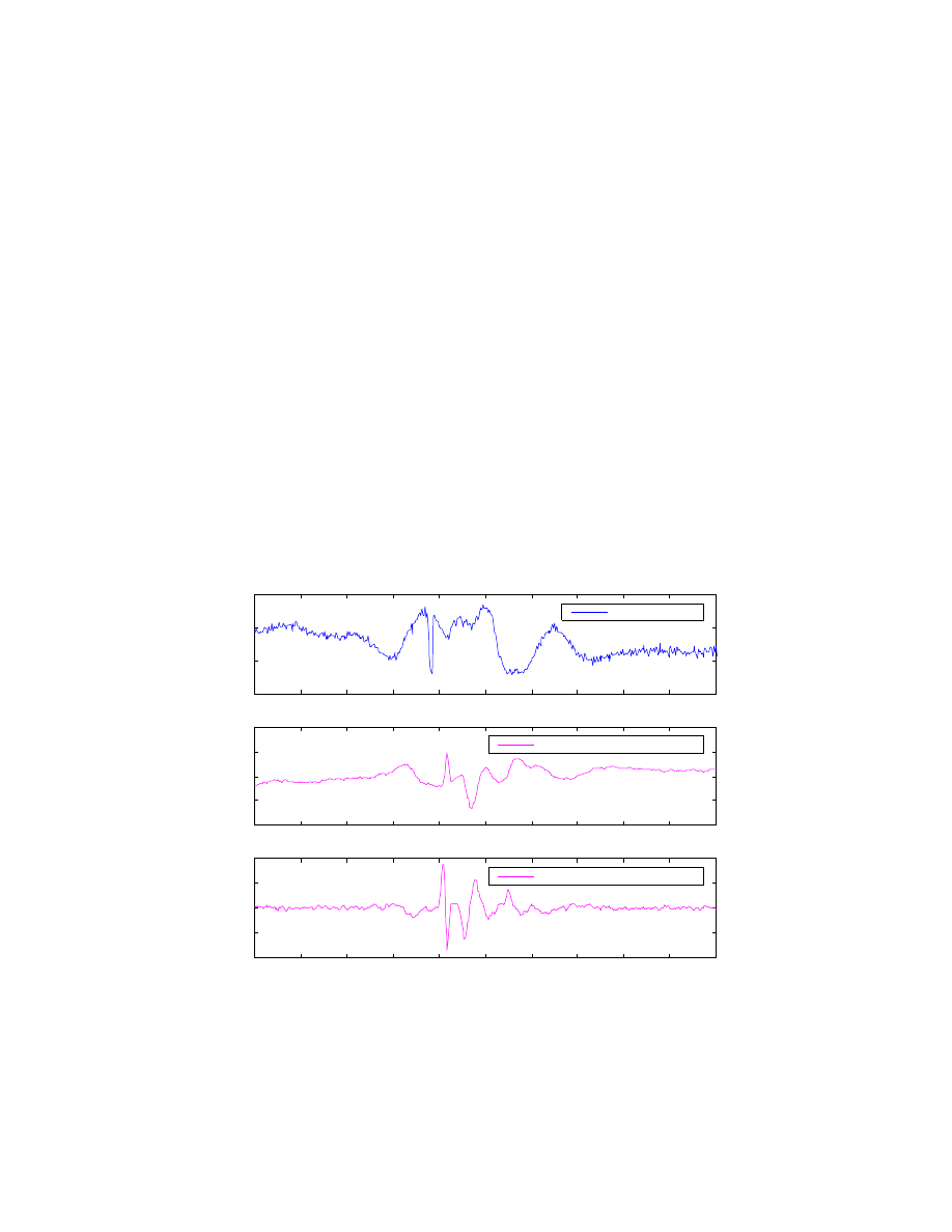
3.2.4

Preview Correction Modifier

Information from the preview buffer will be used to help alleviate the problem observed

in Section 3.2.2. Figure 3.5 shows raw sensor data and the HPR corrected and buffered

road profile. HPR is computed with only road height information. Observe the negative

bump just after the actual bump in the Z

r

plot.

2

2.5

3

3.5

4

4.5

5

5.5

6

6.5

7

0.7

0.8

0.9

1

Range (m)

Simple Preview Correction

Sensor Data

2

2.5

3

3.5

4

4.5

5

5.5

6

6.5

7

−0.1

−0.05

0

0.05

0.1

z

r

(m)

Corrected & Buffered Data

2

2.5

3

3.5

4

4.5

5

5.5

6

6.5

7

−10

−5

0

5

10

z

r

dot (m/s)

Time (sec)

Corrected & Buffered Data

Figure 3.5: Plot of raw preview data and corrected & buffered preview outputs when using

simple HPR computation

24

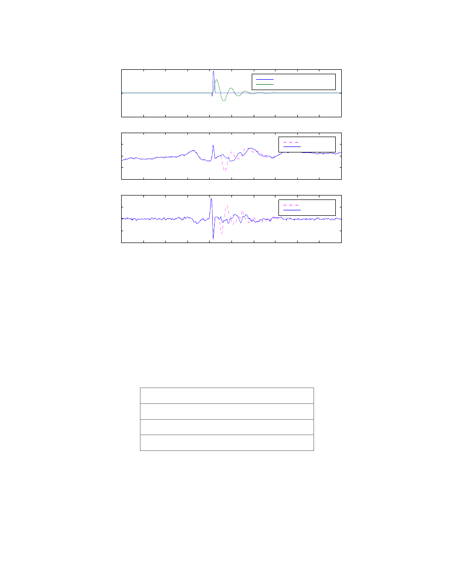
The negative impression can be removed if compensation for tire dynamics is included in

the HPR computation. To do this, bump data is extracted from the buffered preview

information and fed to a quarter car system. Below is the system dynamics derived from

Figure 2.2.

[

]

T

r

r

U

&

=

are the only system inputs and chassis heave

s

x is the output.

(

)

(

)

U

m

c

m

k

X

m

c

c

m

k

k

m

c

m

k

m

c

m

k

m

c

m

k

X

u

t

u

t

u

s

t

u

s

t

u

s

u

s

s

s

s

s

s

s

s

s













































+













































+

−

+

−

−

−

=

0

0

0

0

0

0

1

0

0

0

0

0

1

0

&

[

]

T

u

u

s

s

x

x

x

x

X

where

&

&

=

Figure 3.6: Plant dynamics for tire compensation

Now

s

x is used in the HPR computation and the results are shown in Figure 3.7. MPC

p

places the most weight on

r

Z

&

; in the final plot we see a tremendous improvement over

the original

r

Z

&

.

Results from this technique are promising but extracting the bump data from the preview

information is not a robust process. A better solution is to use this knowledge to modify

the KF and attain better HPR estimates. Thus far, HPR have been computed with LVDT

data (suspension expansion sensor data), as the LVDT correction was much better than

the correction obtained by using the HPR data from the KF.

25

2

2.5

3

3.5

4

4.5

5

5.5

6

6.5

7

−0.05

0

0.05

Preview Correction w/ Tire Compensation

Height (m)

Bump from Buffer

Chassis Response

2

2.5

3

3.5

4

4.5

5

5.5

6

6.5

7

−0.1

−0.05

0

0.05

0.1

z

r

(m)

Original

Modified

2

2.5

3

3.5

4

4.5

5

5.5

6

6.5

7

−10

−5

0

5

10

z

r

dot (m/s)

Time (sec)

Original

Modified

Figure 3.7: Plot of advanced HPR correction data and new preview data

3.3 Kalman Filter

The Kalman Filter (KF) design was done by SSCI. A 14 State, 7 DOF full car model was

used. Below is a list the available vehicle information generated by the KF (bold items

are KF states).

Suspension Expansion

, Suspension Velocity

Hub Velocity

Tire Deflection

Chassis Pitch & Roll rate,

Chassis HPR

Table 3.1: Kalman filter states and vehicle information

Adjusting noise covariances, setting system parameters and validating state information

for the KF was difficult. One subtlety was compensation for the velocity ratio of the

suspension arm. The arm created two coordinate frames, one for the chassis and one for

the wheels and road.

26

3.4 Performance Criterion

The US Army TARDEC has empirically developed a criterion known as “absorbed

power” to quantify ride comfort. This formulation filters the sprung mass acceleration

through a Human Response Filter (HRF) that represents the frequency range most

undesirable by a human driver. A second order approximation of the HRF is given in

equation (3.2), the units of input acceleration are

2

/ s

m

. Output from the filter is squared

and time averaged over a moving window to produce the “absorbed power” measure, also

known as the Cumulative Absorbed Power (CAP). Over a given terrain the CAP should

remain less than 6 Watts for driver comfort. Drivers inherently slow down when the

CAP persistently exceeds the 6 Watt limit.

)

3

.

901

02

.

30

(

12

)

(

F

R

H

2

+

+

=

s

s

s

s

)

(3.2)

27

Chapter 4 - High Level Controllers

Now that the building blocks are explained, the interesting parts of the project can be

readily described. The systems presentation is intended to be an overview of controller

design, references are provided for the interested reader.

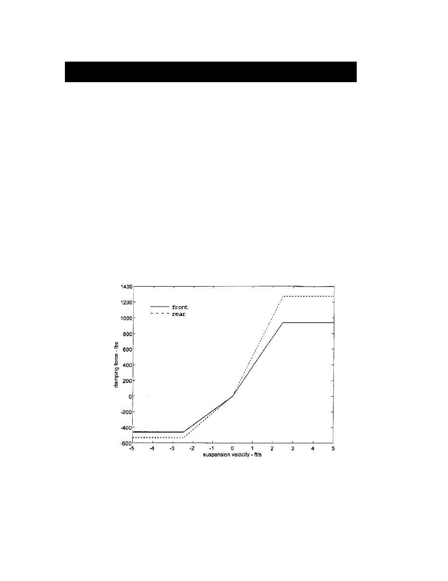
4.1 Mock Passive Suspension

It is difficult to make the actuators naturally behave like a passive suspension. A best

effort approach is to open actuator bypass valves, shut off the hydraulic pump, and set the

primary valve control input to zero. A better method is to use the force mapping

provided by TARDEC for a normal HMMWV suspension. For a given suspension

velocity, the corresponding force is tracked by the FTC – according to Figure 4.1.

Figure 4.1: Plot of damping force vs. suspension velocity for a standard HMMWV

28

4.2 Sky Hook Damping Controller

There are two approaches to sky hook damping:

1. Theoretically add a damper to each wheel

2. Theoretically add three dampers to the chassis, one respectively for HPR

On the HMMWV, the simpler, 4 independent damper method is implemented. The plant

dynamics are derived as follows.

s

s

f

a

s

u

s

s

u

s

ms

x

m

F

F

x

x

k

x

x

c

F

&&

&

&

=

−

+

−

+

−

=

∑

)

(

)

(

Sprung

Mass

Unsprung

Mass

kt

bt

ks bs

F

B

sky

s

s

x

x &,

u

u

x

x &,

r

r &,

Sprung

Mass

Sprung

Mass

Unsprung

Mass

Unsprung

Mass

kt

bt

kt

bt

ks bs

F

ks bs

F

B

sky

B

sky

s

s

x

x &,

u

u

x

x &,

r

r &,

s

s

x

x &,

s

s

x

x &,

u

u

x

x &,

u

u

x

x &,

r

r &,r

r &,

u

u

f

a

u

s

s

u

s

s

u

t

u

t

mu

x

m

F

F

x

x

c

x

x

k

x

r

k

x

r

c

F

&&

&

&

&

&

=

+

−

−

+

−

+

−

+

−

=

∑

)

(

)

(

)

(

)

(

Figure 4.2: Diagram for sky hook damping and standard quarter car equations

The control law is

)

(

s

u

vel

s

sky

des

x

x

K

x

B

F

&

&

&

−

+

−

=

(4.1)

Controller gains are chosen to adjust the pole locations of the original system. For the

HMMWV the gain set {B

sky

, K

vel

} = {2000, 1000} is used.

4.3 Linear Quadratic Regulator

A standard LQR formulation for suspension systems is implemented. The plant

dynamics are of the form used by the Kalman filter. Thus, the cost function includes

29

{Chassis Accel, Susp Travel, Tire Deflection, Pitch & Roll rates, Hub Vel,

Control Usage}

(4.2)

Some transformations are required to put the associated cost function into standard form

and obtain the Riccati equation. The interested reader should consult Thompson et al [19]

for more details.

The LQR weighting set is given in Table 4.1. Very little restriction is placed on the

control input; chassis acceleration, pitch and roll rates have the highest costs. Matlab is

used to generate the LQR optimal matrix gain K.

Parameter

Weight

Chassis Acceleration

10

Pitch & Roll Rate

10

Suspension Travel

1

Hub Velocity

1

Tire Deflection

0.1

Control Usage

5

5

−

e

Table 4.1:

LQR weighting gains

In practice, the output F

des

of the Linear Quadratic Regulator is scaled by 500.

Theoretically, the “control usage” weight could be modified, however the scalar gain is

sufficient.

4.4 Model Predictive Controllers

The MPC was designed and coded for the HMMWV environment by SSCI, source code

and libraries are implemented in Simulink via S-function. MPC is the primary

computation for the 300MHz Alpha processor, at a ∆t of 30ms.

At each sampling instant, the MPC computes a finite number of future control moves

such that a cost function, over a finite horizon, is minimized. The first control output is

fed to the FTC. The exact workings of the MPC involve output prediction (based on a

30

system model) and a receding-horizon approach. For more information on MPC and

MPC

p

formulations consult Gopalasamy et al [9]. Therein, they describe how to recast

the MPC problem to a constrained Quadratic Programming (QP) problem and select the

respective real-time algorithm.

Of interest to this project are the weighting parameters of the cost function. Originally,

the cost criterion was based on the following terms:

{Absorbed Power, Susp Travel, Tire Deflection, Control Usage}

(4.3)

Field testing of the MPC and SKY controllers motivated the addition of an “optimal” sky

hook damping term into the MPC cost function. The ultimate set is

{Absorbed Power, Susp Travel, Tire Deflection, Control Usage, Susp Velocity} (4.4)

The physical constraint set, and respective values are shown below.

{Force, Force Rate, Susp Limit}

(4.5)

With preview information, MPC becomes MPC

p

. MPC

p

enhances MPC by considering

road

Z&

and relative road heights for the desired pH at each wheel.

Parameter

Weight

Absorbed Power

23

Suspension Travel

0.02

Suspension Velocity

192

Tire Deflection

0.08

Control Usage

1.1

6

−

e

Table 4.2:

MPC weighting gains

Constraint

Value

Force

± 8000 N

Force Rate

± 5000 N/s

Suspension Travel

± 0.1 m

Table 4.3:

MPC constraint values

31

Chapter 5 - Experimental Results

HMMWV controllers were introduced systematically, simple controllers were tested first

and computational complexity was slowly increased. Initially, PI position control of the

actuators was used to verify proper hardware wiring and functionality. Force tracking

control was tuned by analyzing the spool voltage surface then later connecting the force

surface to the spool voltage surface. To test the controllers, a desired profile was

required. For this, a custom, relative time, generic profile generator block was created.

Following satisfactory tuning of the FTC, the high-level, force generating controllers

were connected to the desired force of the FTC.

Generated preview information was used with the MPC

p

. Owing to difficulties with the

preview correction algorithm the MPC had not used sensor, preview data at the time of

this report.

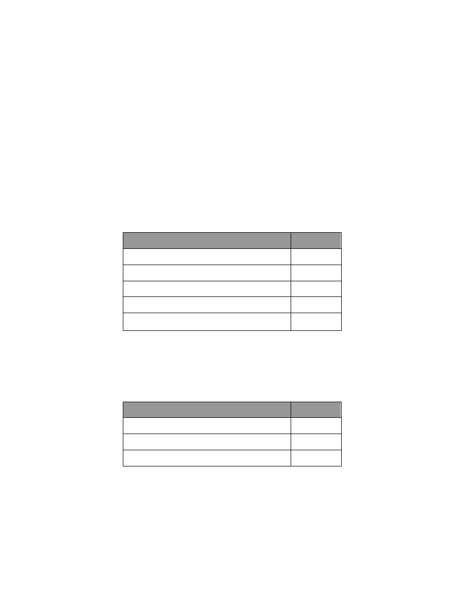
5.1 Ride Height Control

Ride Height Control (RHC) is the most basic, yet essential controller on the HMMWV.

RHC performance is shown in Figure 5.1. The desired position being tracked is part of a

demonstration profile. At the end of a real-time modifiable sequence of events one tire is

raised off of the ground; this demonstrates some extraneous advantages of active

suspension systems.

A slight phase lag is visible in Figure 5.1. The lag can be removed with higher gains but

remains for the sake of passenger comfort.

32

15

20

25

30

−0.04

−0.02

0

0.02

0.04

RHC Performance − LHF

Position (m)

Actual

Desired

15

20

25

30

−0.04

−0.02

0

0.02

0.04

RHC Performance − LHR

Position (m)

Time (sec)

Actual

Desired

15

20

25

30

−0.04

−0.02

0

0.02

0.04

RHC Performance − RHF

Actual

Desired

15

20

25

30

−0.04

−0.02

0

0.02

0.04

RHC Performance − RHR

Time (sec)

Actual

Desired

Figure 5.1: Plot of Ride Height Controller performance

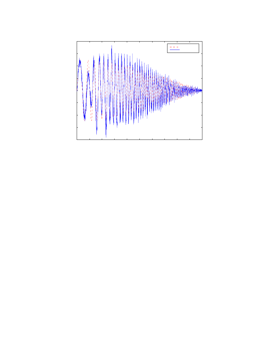
5.2 Force Tracking Control

This section depicts most of the problems mentioned in Chapter 2. The final Force

Tracking Controller (FTC) is more than sufficient for the research objectives. The most

common profile used in tuning the controller is a “sweep sine”. A “sweep sine” varies

frequency linearly from 1Hz to 10Hz and attenuates the amplitude with time. Thus, the

time axis roughly corresponds to a frequency.

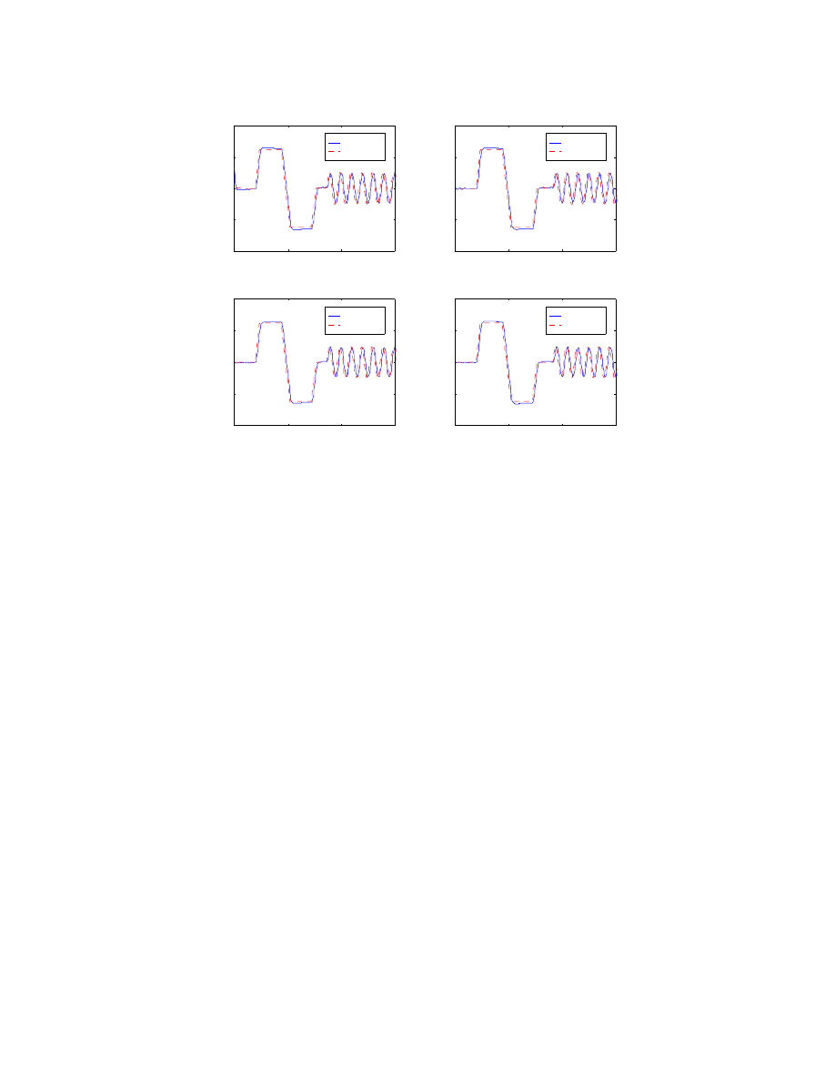
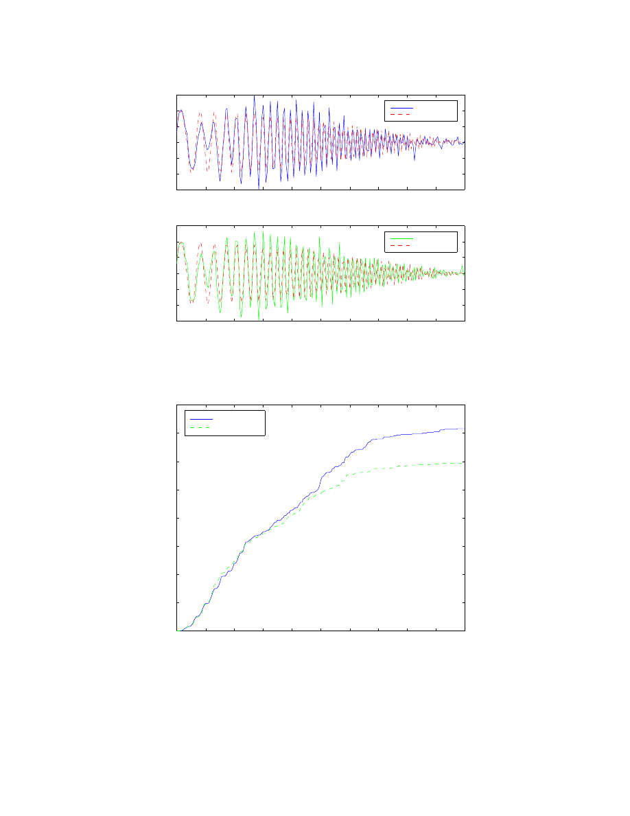
Figure 5.2 shows the affects of the resonant modes of the full car system. To obtain these

plots, FTC gains are turned down slightly to amplify the problem.

33

0

1

2

3

4

5

6

7

8

9

10

−1000

0

1000

FTC HPR Performance − Force (N)

Heave

Actual

Desired

0

1

2

3

4

5

6

7

8

9

10

−1000

0

1000

Pitch

Actual

Desired

0

1

2

3

4

5

6

7

8

9

10

−1000

0

1000

Roll

Time (sec)

Actual

Desired

Figure 5.2: Plot of FTC performance in heave, pitch & roll modes

Observe the resonant peaks of ~ 2Hz for heave and pitch modes; the roll mode is closer

to 4 Hz.

Next are the results of the Output Redefinition scheme. Once again, controller gains are

turned down slightly. There is a slight improvement in tracking around 1.5Hz, or about

1sec, as shown in Figure 5.3. Moreover, Figure 5.4 depicts a mild improvement in the

sum squared relative velocity error for frequencies greater than 5Hz. Relative velocity

error is defined as the difference between the actual suspension velocity

u

s

x

x

&

&

−

and the

velocity predicted by the quarter car model. These results are not an indication that the

theory is erroneous, but rather, the ORD gain cannot be increased very high because

control noise amplification causes system instability. Osorio et al [14] explains that a

gain of 5000 was needed to sufficiently move the poles of the Berkeley Active

Suspension Rig (BASR) system. With the HMMWV FTC and KF only a gain of 150 is

attainable. In implementation, ORD is not used as it requires information from the KF,

which if difficult to obtain given the HMMWV DSP architecture, see Appendices B & C.

34

0

1

2

3

4

5

6

7

8

9

10

−1500

−1000

−500

0

500

1000

1500

Force Tracking Controller Performance

Force (N)

Actual

Desired

0

1

2

3

4

5

6

7

8

9

10

−1500

−1000

−500

0

500

1000

1500

FTC with Output Redefinition

Force (N)

Time (sec)

Actual

Desired

Figure 5.3: Plot of FTC performance with Output Redefinition

0

1

2

3

4

5

6

7

8

9

10

0

0.1

0.2

0.3

0.4

0.5

0.6

0.7

0.8

Relative Velocity Error Improvement using ORD

Sum Squared Error (m

2

/s

2

)

Time (sec)

Kv = 0
Kv = 150

Figure 5.4: Plot of sum squared relative velocity error for output redefinition

35

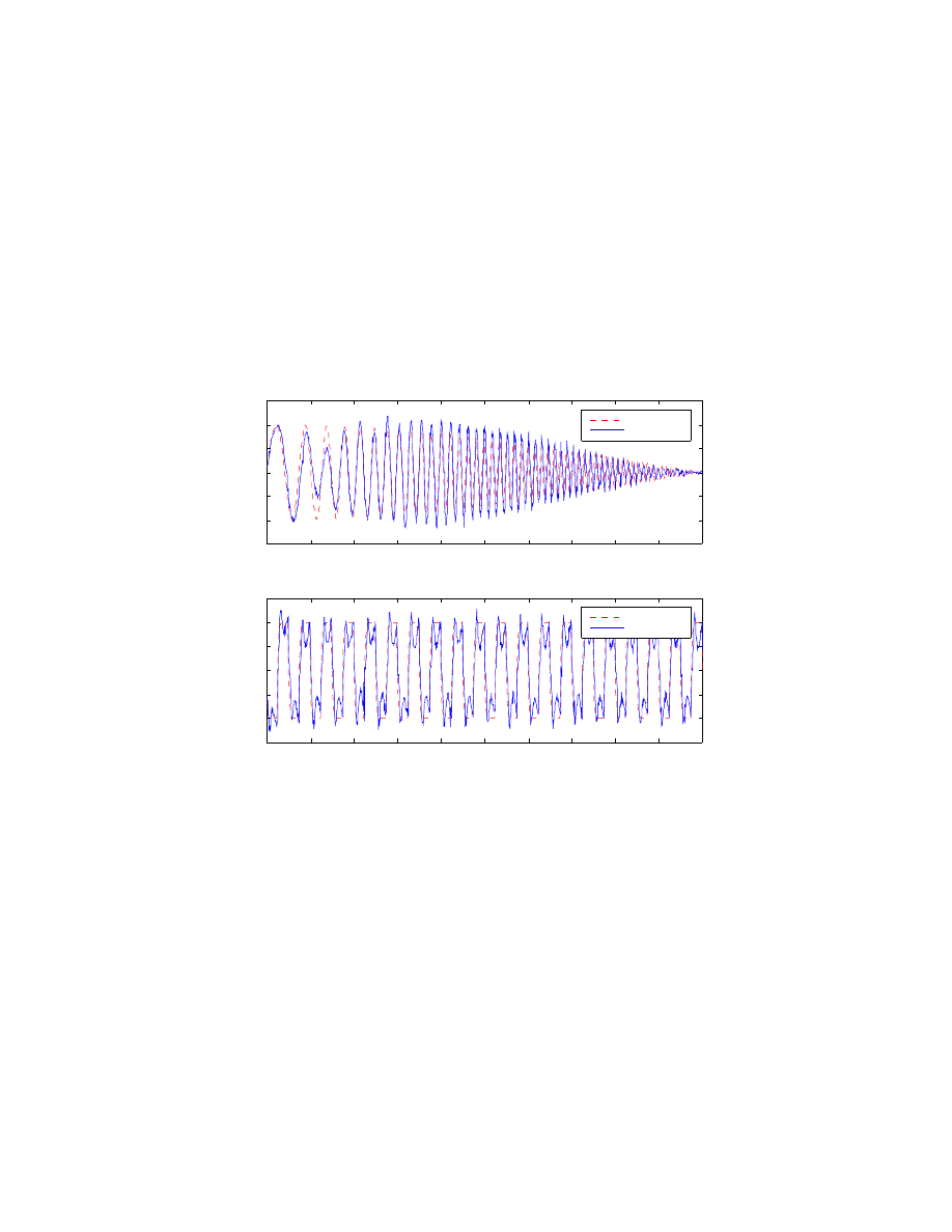
In Figure 5.5 the controller gains are returned to their nominal values and the initial

amplitude of the “sweep sine” was increased to 2000 N. Additionally, the response to a

filtered square wave is shown. There is no compensation for HPR or ORD. If present,

ORD would lessen the dip at each peak.

Figure 5.6 shows FTC performance while tracking a discrete F

des

. Since the higher level

controllers run at a sampling rate of 30ms the original F

des

is filtered, equation (2.24), and

a smoother F

des

is tracked by the FTC.

0

1

2

3

4

5

6

7

8

9

10

−3000

−2000

−1000

0

1000

2000

3000

Force Tracking Control − Sweep Sine

Force (N)

Desired

Actual

0

1

2

3

4

5

6

7

8

9

10

−1500

−1000

−500

0

500

1000

1500

Force Tracking Control − Square Wave

Force (N)

Time (sec)

Desired

Actual

Figure 5.5: Plot of n

ominal FTC performance

36

0

1

2

3

4

5

6

7

8

9

10

−4000

−3000

−2000

−1000

0

1000

2000

3000

4000

Force Tracking Control − Discrete Sweep Sine

Time (sec)

Force (N)

Desired

Actual

Figure 5.6: Plot of FTC performance tracking a discrete, generated control signal F

des

5.3 High-Level Controllers

Tuning and performance evaluation of the high-level controllers is conducted at the test

track described in Appendix D. More realistic performance data is collected on an off-

road, natural terrain.

Figure 5.7 depicts typical results. All of the higher level controllers perform similarly,

the MPC is slightly better than the rest. There is better than a twofold improvement in

the absorbed power criterion when compared to the passive suspension. LQR

performance, not shown, is comparable to the MPC performance. This is true provided

the system remains within constraints, Table 4.3, and there is no preview information.

For the MPC trial in Figure 5.7 the force tracking controller performance is shown.

Observe the two spikes corresponding to collision with the test track obstacles. At these

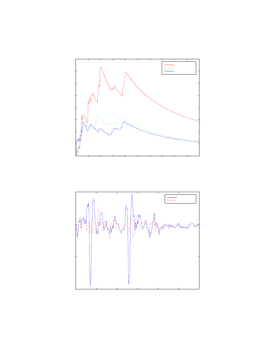
37

instances there is saturation of the control input u

1

. In theory, the MPC

p

should reduce

the amount of saturation.

0

0.5

1

1.5

2

2.5

3

3.5

4

4.5

5

0

5

10

15

20

25

30

35

40

High Level Controller Results − Test Track

Relative Absorbed Power (Watts)

Time (sec)

Passive
Sky Hook
MPC

Figure 5.7: Plot of higher level controller performance evaluated at the test track

0

0.5

1

1.5

2

2.5

3

−10000

−5000

0

5000

FTC Performance, for MPC F

des

− RHF

Force (N)

Time(sec)

Actual

Desired

Figure 5.8: Plot of FTC performance tracking the MPC F

des

of Figure 5.7

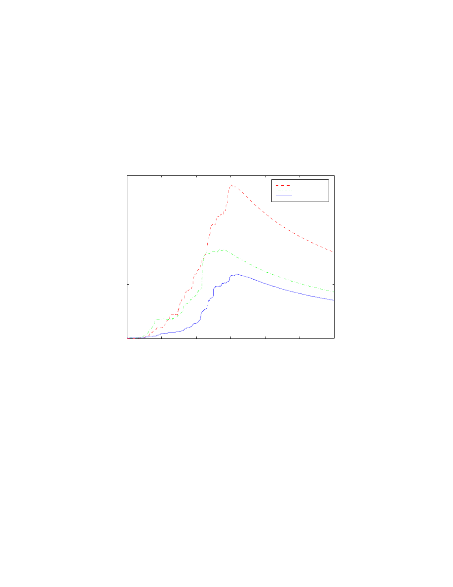
38

Using the same controllers off-road, the results of Figure 5.9 are generated. Now, MPC

handedly beats the Sky Hook Damping controller. Moreover, the off-road results show

that only the MPC maintained a CAP of < 6 Watts. By military standards, this terrain is

only drivable at this speed, 20mph, if the MPC is used.

To better understand the improvements of Figure 5.9 the suspension LVDT

measurements are shown in Figure 5.10. The MPC reduced suspension travel and the

likelihood of suspension saturation, which occurs at approximately ± 0.06 meters.

0

5

10

15

20

25

30

0

5

10

15

High Level Controller Results − Off Road

Cumulative Absorbed Power (Watts)

Time (sec)

Passive
Sky Hook
MPC

Figure 5.9: Plot of higher level controller performance evaluated off-road

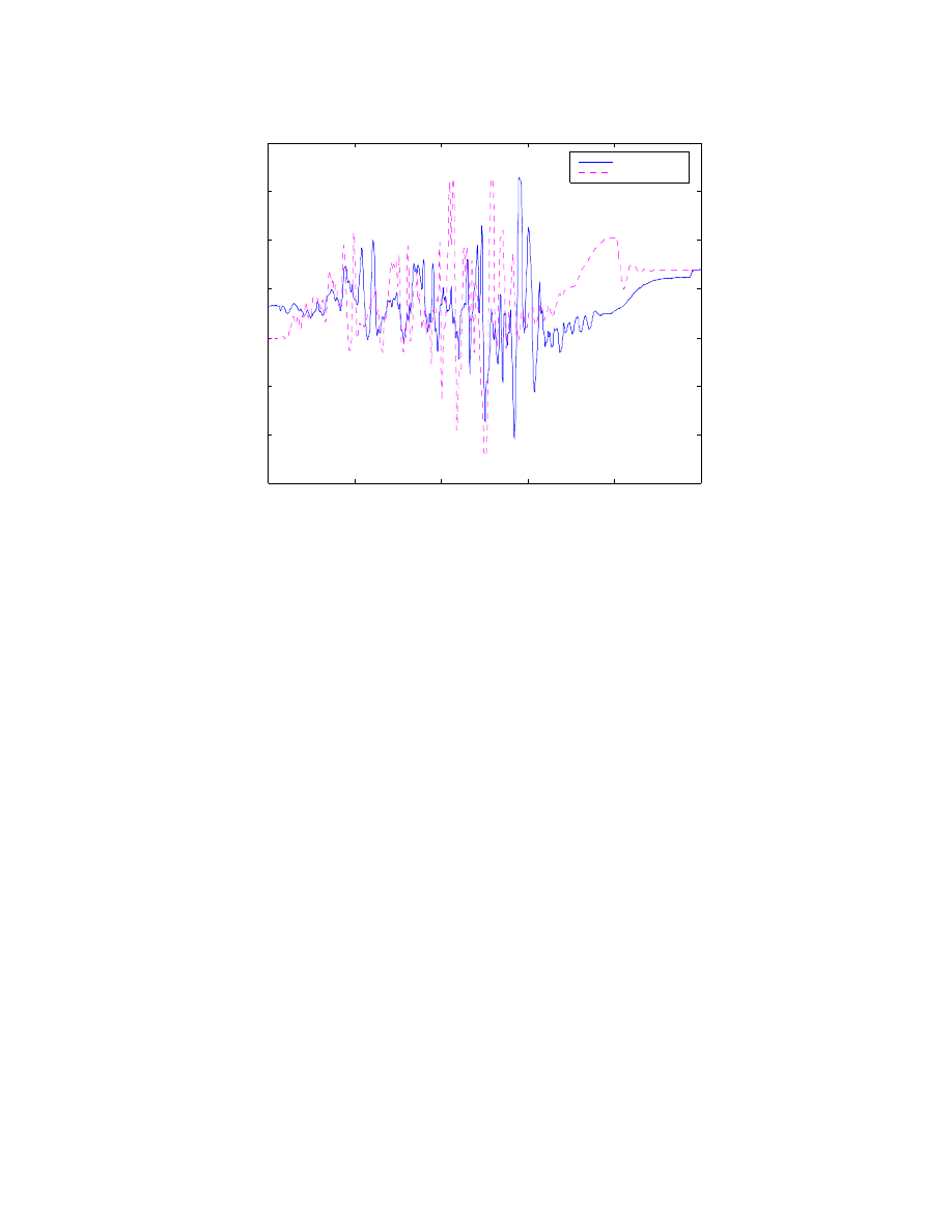
39

0

5

10

15

20

25

−0.06

−0.04

−0.02

0

0.02

0.04

0.06

0.08

LHF Pos (m)

Time (sec)

Suspension Travel for Off−road Test

MPC

Sky Hook

Figure 5.10: Plot of suspension travel for off-road data in Figure 5.9

5.4 MPC Preview Controller

Finally, the preview information is added. Currently, only access to the generated

preview is available. Figure 5.11 implies that with preview, MPC performance

deteriorates. Intuitively this does not make sense. Some possible causes for this are

1. Poor synchronization between digital bumps and real bumps

2. Compounded distance error over the long track, see Figure 3.1

3. Bump profile was to perfect, it has a high initial derivative

Looking into these causes and improving the results is left for future work on the project.

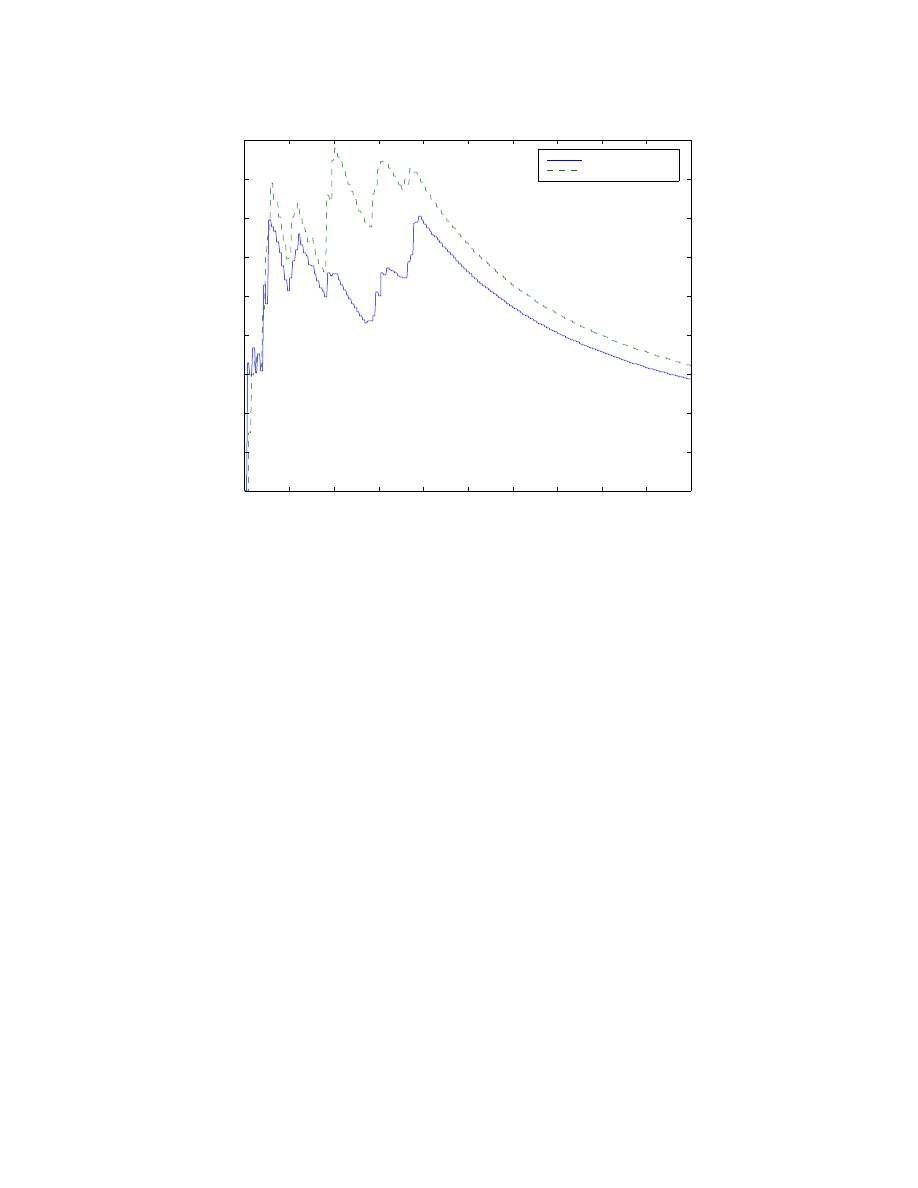
40

0

0.5

1

1.5

2

2.5

3

3.5

4

4.5

5

0

2

4

6

8

10

12

14

16

18

Model Predictive Controller Results − Test Track

Cumulative Absorbed Power (Watts)

Time (sec)

MPC

MPC Preview

Figure 5.11: Plot of MPC performance with and without generated preview data

41

Chapter 6 - Conclusions

Practical, implementation oriented, modifications to dynamic surface control theory were

successfully employed. Modifications involved adding filters at various levels of the

control computation. To the end of realizing full functionality of Model Predictive

Control (MPC) using preview information, numerous subsystems were designed. All

subsystems work well. A Sky Hook Damping Controller (SKY) and a Linear Quadratic

Regulator (LQR) were developed to benchmark the performance of the MPC without

preview. For the non-preview controllers more than a twofold increase in ride comfort

over passive suspension was obtained. This resulted in an increased drivable speed for

rough terrain. In particular, the MPC allowed for the fastest speed over off-road terrain.

All of the infrastructure is in place to test and debug the MPC with preview. Initial

results indicate the need for further research. In specific, more work is needed on the

preview correction algorithm and on the MPC

p

weights and constraints tuning. In the

immediate future testing will continue on the test track. Perhaps an FSLQ with preview

will be implemented; the respective derivation has already been done as part of Phase I

work.

The following support tasks need also be accomplished:

1. Design a test where suspension consistently saturates

2. Compute RMS for test track and compare results to the plot in Appendix D

3. Redesign CAP computation to be based on a moving window of appropriate

size

42

References

[1]

Alleyne, A., “Nonlinear and Adaptive Control with Applications to Active
Suspensions”, Ph.D. Dissertation, University of California at Berkeley, Berkeley,
CA, 1994.

[2]

Alleyne, A., and Hedrick, J.K., “Nonlinear Adaptive Control of Active
Suspensions”, IEEE Transactions on Control Systems Technology, Vol. 3, No. 1,
pp. 94-102, 1995.

[3]

Alleyne, A., and Hedrick, J.K., “Nonlinear Control of a Quarter Car Active
Suspension”, Proceedings of the 1992 American Control Conference, Chicago,
IL, 1992.

[4]

Alleyne, A., and Liu, R., “On the Limitations of Force Tracking Control for
Hydraulic Servosystems”, ASME Journal of Dynamic Systems, Measurement and
Control, 1999.

[5]

Anderson, B., and Moore, J.B., “Optimal Control – Linear Quadratic Methods”,
Prentice Hall, 1990.

[6]

Bender, E.K., “Optimum Linear Preview Control with Application to Vehicle
Suspension”, Trans. Of ASME, J. of Basic Engineering, pp.213-221, Jun.1968.

[7]

Engleman, G.H. and Rizzoni, G., “Including the Force Generation Process in
Active Suspension Control Formulation”, Proceedings of the 1993 American
Controls Conference, San Francisco, CA, pp. 701-705, 1993.

[8]

Gopalasamy, S., and Hedrick, J.K., “Tracking Nonlinear Non-minimum Phase
Systems Using Sliding Control”, International Journal of Control,

Vol

. 57, No. 5,

pp. 1141-1158, 1994.

[9]

Gopalasamy, S., Hedrick, J.K., Osorio C., and Rajamani, R., “Model Predictive
Control For Active Suspensions – Controller Design and Experimental Study”,
Trans. of ASME, J. of Dynamic Systems and Control,

Vol

. 61, pp. 725-733, 1997.

[10] Hac, A., “Optimal Linear Preview Control of Active Vehicle Suspension”,

Vehicle System Dynamics, Vol. 21, pp. 167-195, 1992

[11] Hac, A., “Suspension Optimization of a 2-DOF Vehicle Model Using Stochastic

Optimal Control Technique”, Journal of Sound and Vibration, Vol. 100, No.3,
pp.343-357, 1985.

[12] Hrovat, D., “Survey of Advanced Suspension Developments and Related Optimal

Control Applications”, Automatica, Vol.33, No.10, pp 1781-1817

43

[13] Langlois, R.G., and Anderson, R.J., “Preview Control Algorithms for the Active

Suspension of an Off-Road Vehicle”, Vehicle System Dynamics, Vol. 24, pp.65-
97, 1995.

[14] Osorio, C., Gopalasamy, S., and Hedrick, J., “Force Tracking Control for Electro

hydraulic Active Suspensions Using Output Redefinition”, Proceedings of the
ASME Winter Annual Meeting, Nashville, TN, 1999.

[15] Rajamani, R., “Observers for Nonlinear Systems, with application to Automotive

Active Suspensions”, Ph.D. Dissertation, University of California at Berkeley,
Berkeley, CA, 1993.

[16] Sharp, R.S., and Hassan, S.A., “The Relative Performance Capabilities of Passive,

Active, and Semi-Active Car Suspension Systems”, Proceedings of the Institution
of Mechanical Engineers, Part D, Vol. 203, No.3, pp.219-228, 1986.

[17] Slotine, J.J., and Li, W.P., “Applied Nonlinear Control”, Prentice Hall, 1991.

[18] Thompson, A.G. and Chaplin, P.M., “Force Control in Electrohydraulic Active

Suspensions”, Vehicle System Dynamics, Vol. 25, pp.185-202, 1996.

[19] Thompson, A.G., Davis, B.R., and Pearce, C.E.M., “An Optimal Linear Active

Suspension with Finite Road Preview”, Society of Automotive Engineers paper
0148-7191/80/0225-0520(800520), 1980.

[20] Tomizuka, M., “Optimum Linear Preview Control with Application to Vehicle

Suspension – Revisited”, Trans. of ASME, J. of Dynamic Systems, Measurement
and Control, Vol.98, No.3, pp.309-315, Sep.1976.

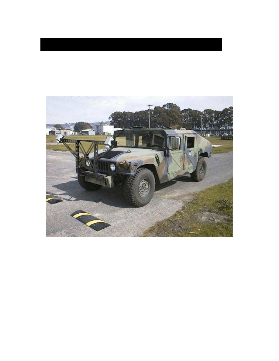
44

Appendix A - HMMWV Hardware

A.1 Equipment as Received

Vehicle

Figure A.1: Photograph of experimental HMMWV

The vehicle used for this project is an experimental High Mobility Multi-Purpose

Wheeled Vehicle (HMMWV) Model M1026, manufactured in 1993 by American Motors

General for the US Army TACOM. Powered by a 6.5 liter diesel V8 rated at 150 hp @

3600 RPM, the HMMWV has a top speed of 55 mph. The engine is mated to an

automatic transmission driving a full time four-wheel drive system.

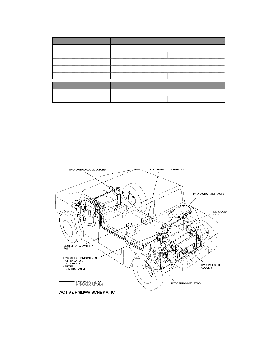
45

Dimensions

Front

Rear

Wheelbase
Distance from CG

1531.6mm

1770.4mm

CG Height
Track
Total Suspension Travel

269mm

271.5mm

Weights

Front

Rear

Gross Vehicle Weight
Unsprung Weight

126Kg

130Kg

3302mm

842.6mm

1818.6mm

3810Kg

Table A.1: Base Vehicle Data

Hydraulic System

Lotus Engineering of England modified the vehicle for the Army’s research purposes.

The conversion work was done in 1993, under a previous contract with Lotus for the

development and implementation of a velocity based active suspension controller.

Figure A.2: Physical schematic for the experimental HMMWV

46

As can be seen by the schematic in Figure A.2, the experimental HMMWV has been

equipped with four hydraulic actuators in place of the standard passive suspension shock

absorbers. The vertical wheel travel was nearly doubled to 26 centimeters.

A Vickers PV3-115 hydraulic pump powers the system hydraulics. The pump is rigidly

mounted to the chassis and is driven by a transmission belt directly connected to the

engine powertrain. The system supply pressure is 3000 psi. With a maximum design

flow of 45 liters per minute, the pump consumes up to 32 hp and requires an engine speed

of 700 to 3500 rpm. This information is summarized in Table 1.1.

Two independent current driven electro-hydraulic servovalves control hydraulic flow in

each of the four actuators. Moog, Inc., located in the United Kingdom, manufactured

these valves. The primary spool valve, model E773-030, controls the amount and

direction of flow to or from each of the two actuator chambers. The bypass valve, model

E760-730, controls the area of an orifice that allows flow between the two chambers of

the actuator. While the primary spool valve controls the actuator behavior by introducing

energy to the system, the bypass valve can only control the rate of energy dissipation

within the actuator. See actuator schematic, Figure 2.3.

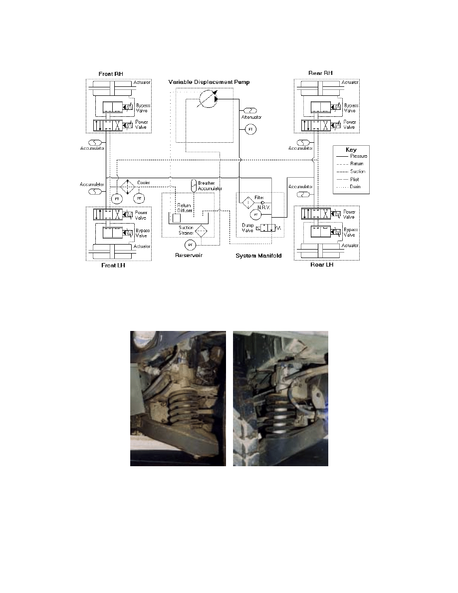
47

Figure A.3: Schematic for the HMMWV hydraulic system

Figure A.4: Photographs of hydraulic actuator installations: left- Front right- Rear

48

Sensors and Electronics

The Lotus-modified HMMWV is equipped with a suite of sensors and transducers to

measure various vehicle data. Table A.2 lists the Lotus-installed sensors and their

respective measurements.

Qty Sensor Type

Location

Measurement

4

Load Cell

Top mount of each actuator

Actuator forces

4

LVDT

Inside each actuator

Actuator displacement

4

Hub Accelerometer

On each wheel hub

Axle vertical acceleration

2

CG Accelerometer

CG pack

Longitudinal & lateral accel.

1

Yaw Rate Sensor

CG pack

Vehicle yaw rate

1

Rack Displacement

Steering box pinion shaft

Steering angle

1

Speedometer

Engine compartment

Vehicle speed

1

Tachometer

Engine compartment

Engine rpm

3

Pressure Transducer Pump outlet, filter inlet & outlet

Supply pressures

2

Pressure Transducer Cooler inlet & outlet

Return pressures

1

Pressure Transducer Reservoir Tank

Reservoir pressure

1

Hydraulic Flow
Meter

In-line after pump

Total hydraulic flow

3 Thermocouple

Reservoir, pump outlet, &
cooler inlet

System temperatures

Table A.2: Experimental HMMWV, Lotus installed sensors and transducers

Sensor and transducer signals are connected to the Lotus Interface and Signal

Conditioning Box, Figure A.5, located in the center console of the HMMWV. Most

measurements are passed through a set of differential gain amplifiers and low pass, anti-

aliasing filters with a cut off frequency around 250Hz. The Lotus Interface and Signal

Conditioning Box receives power directly from the car battery, 24 VDC, and provides

regulated power (

±

15, +12 or +5 VDC) to all connected sensors.

49

Figure A.5: Photograph of Lotus interface and signal conditioning box

A.2 Sensors added by UCB

As received, the sensing and control capabilities of the HMMWV were insufficient to

obtain our control objectives. The following subsections detail UCB modifications.

A.2.1 Servo

Amplifiers

The output power of the digital to analog converter (DAC) was insufficient to control the

primary and spool valves directly. Eight servo-amplifiers were purchased and are used in

a proportional-derivative (PD) current feedback loop to position the respective spools.

These boards allow control of the spool via a voltage signal from the AutoBox as well as

provide for a voltage feedback term proportional to the physical position of the spool.

Below is the specification sheet for the amplifiers. Capacitor C1 was removed to

eliminate the integral component of the controller. Resistor R7 was changed to adjust the

proportional gain of the current feedback servo amplifier controller.

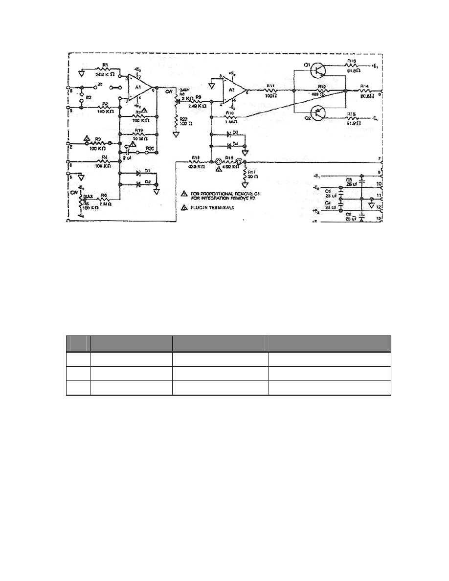
50

Figure A.6: Schematic for the servo-amplifier circuit board

A.2.2

Accelerometers & Gyros

In addition to the vehicle sensors installed by Lotus, eight new sensors were installed.

Four sensors to measure additional states and four to replace faulty sensors, see Table

A.3. All sensors were manufactured by CFX, Edgemont PA. A specification sheet for

each type of sensor is provided in Figure A.7.

Qty Sensor Type

Measurement

Mount Locations

2

Accelerometer

Z-axis acceleration

Opposite corners of the chassis

2

Rate Gyro

Pitch and Roll rates

Center console

4

Accelerometer

Hub Accelerations

Inner hub (replaced old sensors)

Table A.3: Additional vehicle sensors installed by UCB

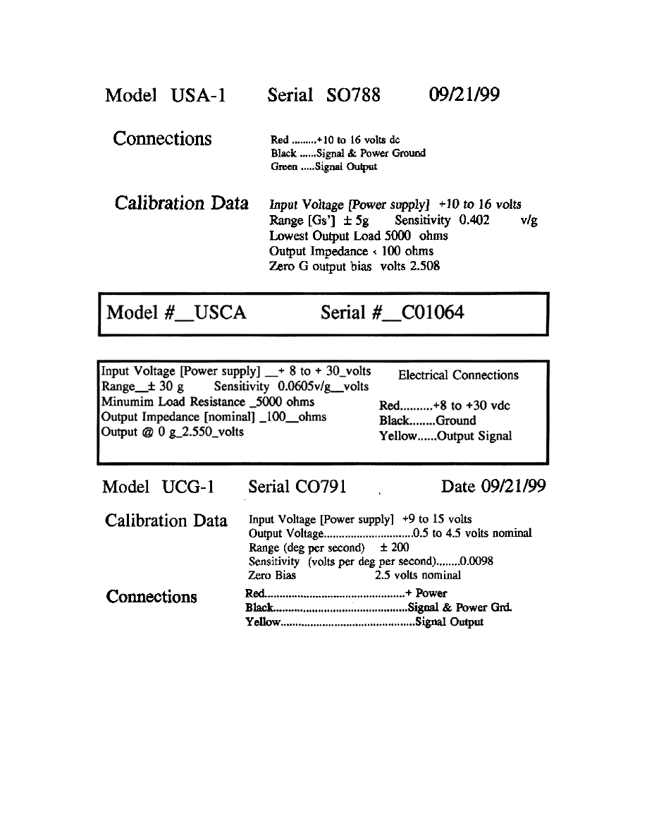
51

Figure A.7: Specification sheets for UCB added vehicle sensors. top- chassis accelerometer

middle- hub accelerometer bottom- rate gyro

A.2.3 Preview

Sensors

For relatively straight path motion or for uniform, wide bumps in the road profile it is

sufficient to use only range finding units to obtain preview information. This assumption

52

simplifies the sensor requirements and, as shown in Section 3.2.2, the preview processing

algorithm.

Two types of sensors were explored:

1. Frequency Modulated Continuous Wave (FMCW) radar by O’Conner

Engineering

2. WTA24-P5401 LED optical sensor by Sick Optic

FMCW Radar Sensor

The FMCW radar has a central frequency of 24.5 GHz and scanning range of 0.5 GHz.

For easy comparison with the WTA24, the other pertinent information is presented in

Table A.4.

Specification:

Nominal Value:

Range

1.0 m - 5.0 m

Range Rate

0 m/s - 40 m/s

Resolution

0.01 m

Reproducibiliy

-

Accuracy

-

Light Spot

0.3 m - 0.6 m

Output

2.5 V - 7.0 V

Response Time

1.1 ms

Table A.4: FMCW radar specifications.

WTA24 Optical Sensor

This sensor consists of a modulated infrared LED, with an average life of 100,000 hours

at 25

°

C, and precision reflectors all mounted inside a rugged diecast metal housing. The

unit meets or exceeds shock and vibration standards: IEC 68-2-27/IEC 68-2-6. The

general specifications of interest are tabulated below:

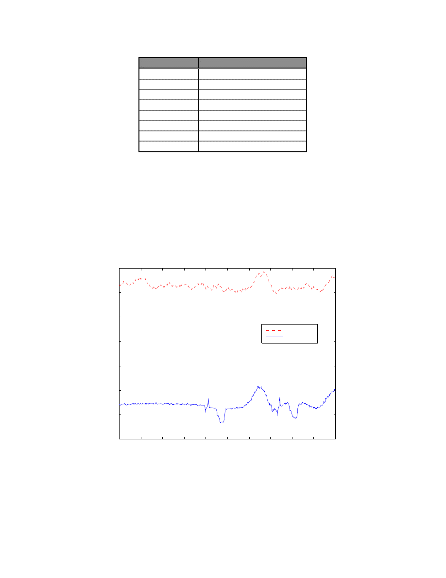
53

Specification:

Nominal Value:

Range

0.6 m - 1.2 m

Range Rate

-

Resolution

0.02 m

Reproducibiliy

0.03 m

Accuracy

0.08 m

Light Spot

0.02 m - 0.03 m

Output

4 mA - 20 mA

Response Time

5.0 ms

Table A.5: WTA24-P5401 optical sensor specifications.

Typical sensor outputs are shown in Figure A.8. The optical sensor detects small bumps

better that the radar, as in the top plots. However, since the radar filters small width, low

frequency disturbances it may better represent the actual system disturbance; tire berth

naturally filters low amplitude disturbances of that type. Bottom plots depict this

phenomenon well around 4.5 seconds.

0

0.5

1

1.5

2

2.5

3

3.5

4

4.5

5

0.6

0.8

1

1.2

1.4

1.6

1.8

2

Time (sec)

Range (m)

Calibrated Sensor Data − Target: Parking Curbs

Radar
Optical

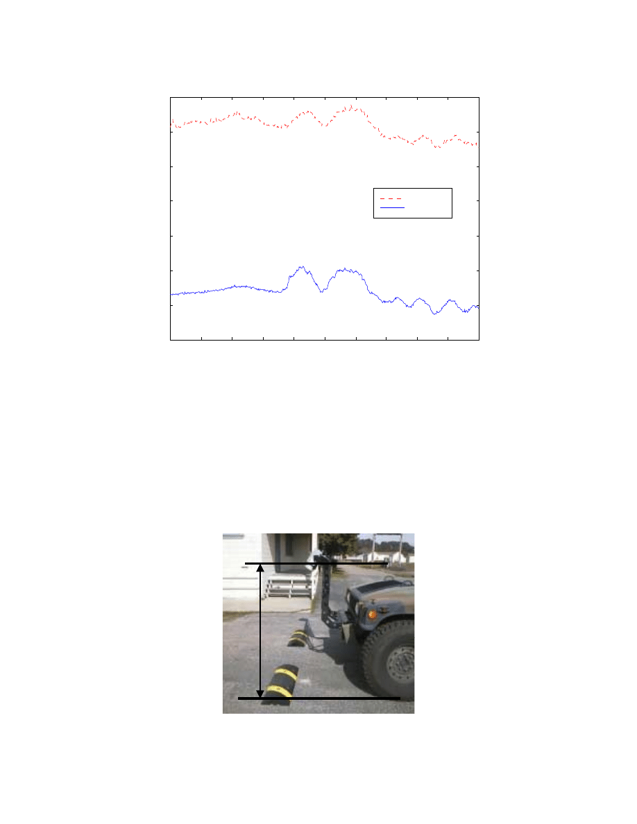
54

0

0.5

1

1.5

2

2.5

3

3.5

4

4.5

5

0.6

0.8

1

1.2

1.4

1.6

1.8

2

Time (sec)

Range (m)

Calibrated Sensor Data − Target: Off Road / Dirt

Radar
Optical

Figure A.8: Plots of preview sensor comparison: top- Parking curbs, slow bottom- Dirt road,

moderate speed

A.3 Sensor Mount

A custom designed, steel metal frame rigidly attached to the front bumper of the

HMMWV was the original mount, see Figure A.9.

0.6m

1.5m

Figure A.9: Photograph of original radar mount with key dimensions labeled

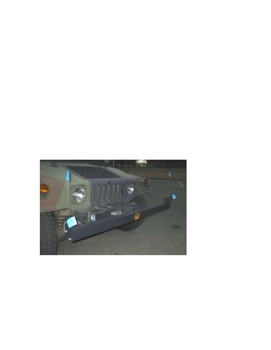
55

The mount had adjustable radar mount angles (to change the preview distance), strong

structure to endure rugged terrain, high natural frequency to minimize signal noise, and

right angle protrusion to allow the hood to open.

A new mount was designed and built to hold the optical sensors and radar as well as to

modify some features of the original mount paradigm. With the new mount, the drivers

view is not obstructed and the radars are 1 foot higher. The new mount is not as rigid as

the original and changing the preview angle requires construction of additional fixtures,

see photo below. Mount preview characteristics are:

► 9, 0.01 sec steps of preview

► 35 mph maximum vehicle speed

► ~2 samples/ft minimum at 100Hz buffer processing

Figure A.10: Photograph of new, wooden, preview mount in WTA24 configuration

Radar mounts, not shown, allow for vertical, side mount of the radar. Essentially, the

radar looks straight down at a road profile different than the profile under the wheels.

This assisted in application testing of the radar.

56

Appendix B - Signal Processing

A dSpace Autobox is used as the HMMWV control computation computer. Prior to

entering the Autobox some signals require pre-filtering or amplification. The particular

sensor and signal routing configuration determine the type of analog signal processing

required. For instance, noise from the spool position feedback signal was corrupting all

servo-amplifier data on the cable; now, an analog low pass filter is applied prior to

assembling the signals.

Every sensor signal is routed through the center console of the HMMWV. Thus, most of

the analog signal conditioning is computed there. Signals enter the Autobox via a 32-

wire flat ribbon cable.

B.1 Autobox

The development and real time implementation is done using a dSpace multiprocessor

data acquisition and Digital Signal Processing (DSP) unit, which consists of:

I/O Boards:

DS2003: 32 Channel Analog to Digital Converter Board

DS2103: 32 Channel Digital to Analog Converter Board

Digital Signal Processing Boards:

DS1003: TI TMS320C40 Parallel 60MHz DSP board

DS1004: DEC Alpha AXP21164 300MHz DSP board

Expansion Box for In-Vehicle Experiments:

Autobox

dSpace Software Tools:

Cockpit: Virtual Instrument Panel Tool

Trace: Data Acquisition and Variable Display Tool

RTI-MP: Multiprocessor Real time interface for Matlab and
Simulink

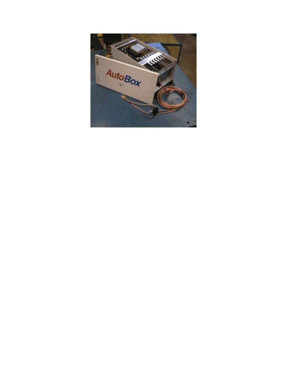
57

Figure B.1: Photograph of AutoBox expansion housing for in-vehicle experiments

The expansion box is specifically designed for in-vehicle experiments and houses all four

dSpace boards. The Autobox receives power directly from the vehicle battery, 24 volts.

Internal DC/DC power supplies regulate power and compensate for any voltage

fluctuations. Interface to a Notebook PC is made via Ethernet cable. The Notebook PC

is used for programming, downloading the control code to the DSP boards and, if desired,

for data acquisition and display. Although the downloaded control code is fully

autonomous, the PC interface is used to change control modes. Figure B.2 depicts the

basic hardware architecture of the dSpace data acquisition and DSP unit.

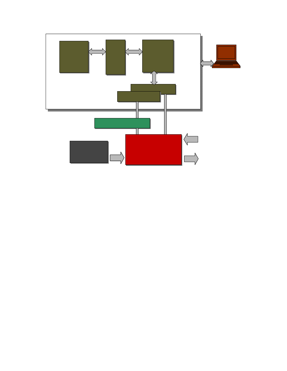
58

From

HMMWV
Sensors

To

HMMWV

Actuators

Servo Amplifiers

Lotus Interface &

Signal Conditioning

Box

UC Berkeley

Sensor

Interface

Auto

Box

ADC Board

IO Boards

DS2003
DS2103

DAC Board

DS1004

Alpha

21164

300 MHz

DS1003

TMS320C40

60 MHz

Dual

Port

RAM

PC

From

HMMWV
Sensors

To

HMMWV

Actuators

Servo Amplifiers

Servo Amplifiers

Lotus Interface &

Signal Conditioning

Box

Lotus Interface &

Signal Conditioning

Box

UC Berkeley

Sensor

Interface

UC Berkeley

Sensor

Interface

UC Berkeley

Sensor

Interface

Auto

Box

ADC Board

IO Boards

DS2003
DS2103

DAC Board

DS1004

Alpha

21164

300 MHz

DS1003

TMS320C40

60 MHz

Dual

Port

RAM

Auto

Box

ADC Board

IO Boards

DS2003
DS2103

DAC Board

DS1004

Alpha

21164

300 MHz

DS1003

TMS320C40

60 MHz

Dual

Port

RAM

Auto

Box

Auto

Box

ADC Board

IO Boards

DS2003
DS2103

DAC Board

ADC Board

ADC Board

IO Boards

DS2003
DS2103

DAC Board

DAC Board

DS1004

Alpha

21164

300 MHz

DS1004

Alpha

21164

300 MHz

DS1003

TMS320C40

60 MHz

DS1003

TMS320C40

60 MHz

Dual

Port

RAM

Dual

Port

RAM

PC

PC

PC

Figure B.2: Diagram of the hardware architecture for active suspension control

All connections to the Autobox are routed through the Lotus Interface Box. The box

provides two pre-established 32pin connectors for the I/O cables. Inside the AutoBox

the I/O boards are connected to the C40 DSP by a peripheral high-speed bus (PHS-bus).

The C40 DSP board processes the I/O, FTC and communication tasks, the Alpha 21164

DSP board is used for complex floating point operations and computationally intensive

processes such as the MPC and preview buffer. Data is transferred between the C40 and

the Alpha via dual-port memory, allowing for fast interrupt-driven communication

channels. A PC connects to the system via Ethernet cable and provides a graphical user

interface for monitoring and interacting with the application running on the system.

Graphic interaction with the real-time application is performed with the dSpace Cockpit

and Trace tools.

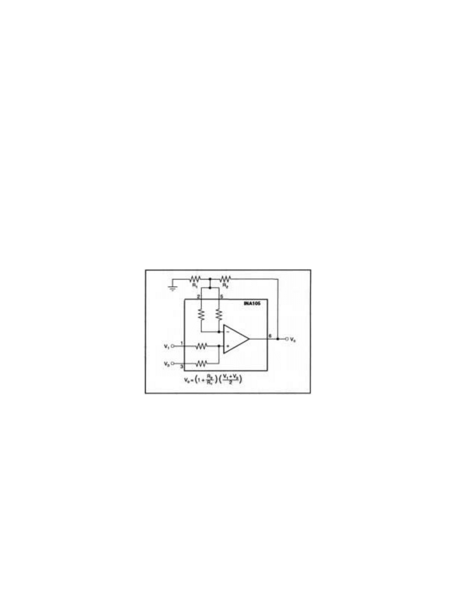
59

B.2 Signal Conditioning

Prior to connecting sensor signals to the Autobox it is necessary to filter or amplify some

signals. Inside the Lotus box the signals pick up about 100mV of noise; to maintain a

good signal to noise ratio the respective sensor signals are pre-amplified before the Lotus

box.

When allowable, only software filters are used to ensure uniform phase delay in signals

and also to allow for easy modification of cutoff frequencies.

Hardware Amplifiers & Filters

A sample schematic for the WTA24 preview sensor preamplifier is given in Figure B.3.

In this case, the amplified voltage output (converted from current output) exceeded ±10

volts, but not the 20 volt range, of the ADC so a bias is added during the amplification

stage.

Figure B.3: Schematic for the summing amplifier used for the WTA24

Software Filters

When necessary 40Hz low pass butterworth filters are used. The filter design can be

obtained via the Matlab, “butter” command. No bias removing filters are implemented

on sensor inputs. Static subtraction of sensor bias is sufficient for short term testing.

60

Appendix C - Real-time Software

For the purposes of prototyping, software is the ideal platform as it affords easy

modification. To comply with the requirements of the dSpace compilers, Matlab, by

Math Works Inc., was chosen as the programming language. The real-time interface

multiprocessor (RTI-MP) tool provides automatic code generation directly from Simulink

block diagrams and renders low-level C programming unnecessary. Simulink is a

graphical interface to the Matlab software. When practical, code is written graphically

using existing Simulink components from standard libraries. Upon occasion it is

necessary to construct custom blocks of code, S-functions, to perform complicated

functions, such as the MPC and the preview buffer algorithms.

This Appendix is intended as a User’s Guide to the HMMWV software.

C.1 dSpace/Simulink Environment

Versions

Matlab

Version: 5.1.1.4

Date: September 2, 1997

Toolboxes:

Simulink Fuzzy

Logic*

Real-Time Workshop (RTW) Mu-Analysis and Synthesis*

Signal Processing

System Identification*

Control System

QFT Control Design*

dSpace Libraries

Partial Differential Equation*

Nonlinear Control Design*

* Installed but not necessary in the current implementation.

Table C.1: Matlab version and installed toolboxes

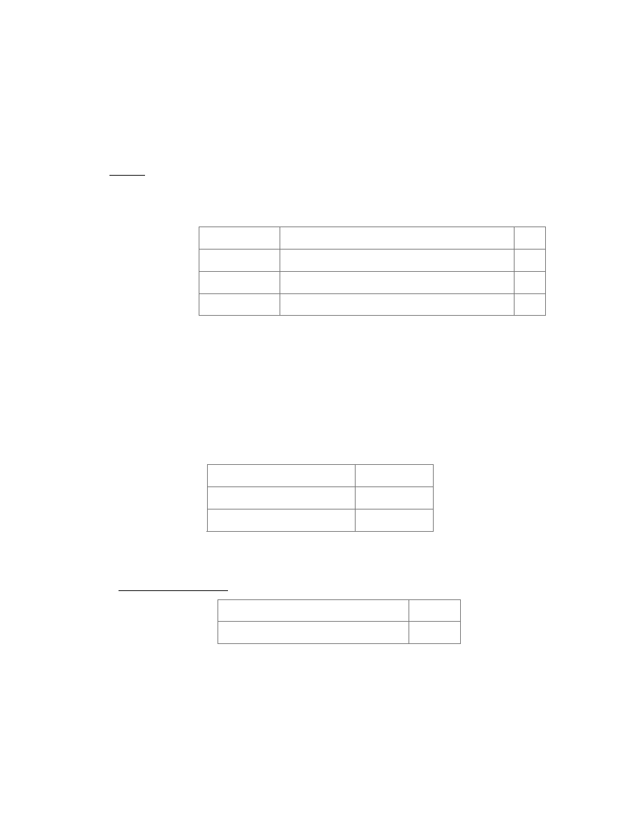
61

To obtain the version listed above, version 5.1.1 was installed and a Matlab provided

update program was run. In addition to the toolboxes above, the “State Flow” toolbox

would be useful. One of the primary functions of the code is to change the states of the

controller; pre-defined state transition software would have aided greatly in this regard.

dSpace

Version: 1.3

Build #: 1998110901

Components:

RTI1003

Real-Time Interface to Simulink

3.2

RTI-MP

RTI for Multiprocessor Systems

3.2

MLIBN

Matlab-DSP Interface Library

3.1

MTRC40N

Real-Time Trace Module for Matlab

3.1

Table C.2: dSpace version and components

During the course of the project dSpace version 2.1 was received. Due to some slight

bugs, the new software was never used for HMMWV control.

Configurations

Hardware configurations and setup parameters for the boards are set according to the

dSpace documentation. A summary of the important settings is provided below:

IP address of Autobox:

128.32.14.44

I/O Address for DS1003:

318-31F

h

I/O Address for DS1004:

310-317

h

Table C.3: Hardware addresses

DS2003 A/D Settings

Hardware:

PHS-Bus Base Address:

20

h

DIP-Switch Setting:

0010

Software:

±

10 V, 15 bit resolution on all functional channels. All 32

channels are used.

Table C.4: ADC settings

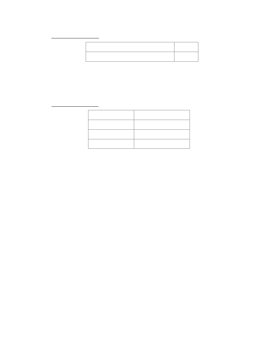
62

DS2103 D/A Settings

Hardware:

PHS-Bus Base Address:

90

h

DIP-Switch Setting:

1001

Software:

±

10 V, 14 bit resolution on all functional channels. Only odd

numbered channels 5-19 are used. Upon initialization,
termination, and errors the output voltage is set to zero.

Table C.5: DAC settings

Multiprocessor Setup

Scheduler mode: multiple timer tasks

Basic step size: 0.001 sec

DS1003 Solver: ode4

DS1004 Solver: discrete

Table C.6: Multiprocessor information

To determine the best paradigm for data relay across the dual port memory, see below,

application tests were conducted. From the results: the Alpha board runs a 10ms and

30ms task only and data transfer from the TI board to the Alpha board is conducted via

virtual shared memory. Data transfer from the Alpha board to the TI board is conducted

via swinging buffer.

Swinging buffer – data is written to the buffer and not overwritten until all of the data

from one write process is read. This method guarantees congruent data but requires 3

times the storage space.

Virtual shared memory – data read and write processes occur when the respective process

is ready to read or write. Data is not guaranteed congruent but no additional memory

space is required.

More information on the protocols is given in the dSpace documentation.

C.2 Implementation Architecture

Below is the system level block diagram of the HMMWV implementation. Graphically,

the components of the control software are divided into several subcategories: input

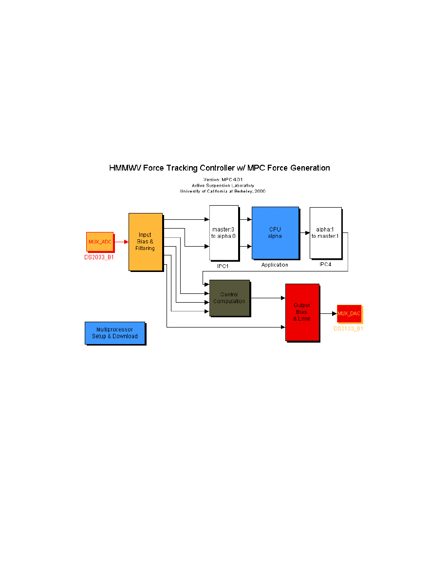
63

processing, control computation, output processing and alpha processes. There are two

types of blocks, program blocks and hardware interface blocks. Program blocks, e.g.

“Input Bias & Filtering” and “CPU alpha”, use standard Simulink programming practices

to implement the control. Hardware blocks, e.g. “MUX_ADC” and “master:0 to

alpha:0”, are provided by dSpace and handle the reading and writing of data to the

respective boards. After a general overview of the program structure, the following

sections will detail the logic underneath the custom program blocks.

Figure C.1: Simulink model of the system implementation

The set of 32 input signals is read from the ADC card onto the TI board. These signals

are then calibrated, grouped, and filtered. From there some signals are transferred to the

Alpha board via the dual port memory blocks. Other signals remain on the TI board and

are connected to the control computation block. After the control algorithm computes the

desired spool voltage, the 4 command signals are passed through a safety and limit check

before being transferred to the DAC. Bypass valve status is set within the “Output Bias

& Limit” block. The “Multiprocessor Setup & Download” block is a graphical way to

call the build and download commands for the system.

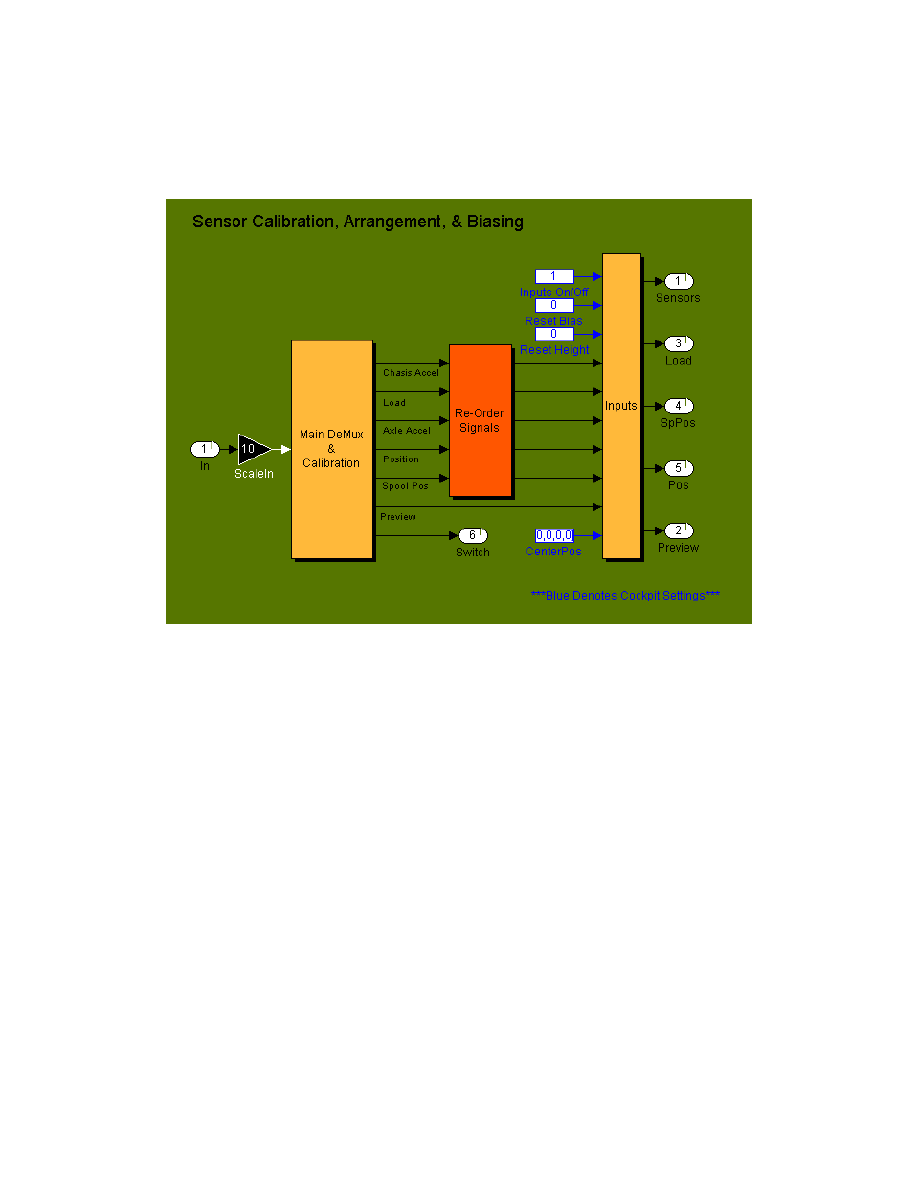
64

C.2.1

Signal Processing Modules

Input Processing

Figure C.2: Simulink model of underneath the “Input Bias & Filtering” block

Signals received and sent to the ADC/DAC are an order of magnitude less than the

physical, measured signal. After scaling the input, the signals are calibrated according to

specification documents and grouped with like signals. The sensor inputs are not ordered

in a consistent manner, the “Re-Order Signals” block puts all data in the sequence:

1. LHF – Left Hand Front

2. LHR – Left Hand Rear

3. RHF – Right Hand Front

4. RHR – Right Hand Rear

Thus creating a standard numbering order for the actuators. The “Inputs” block contains

all of the signal filters and bias subtraction schemes.

At this stage the pseudo state transition methods become evident. Constant values of 0 or

1 are used to turn certain features on or off. The value of 1 or 0 can be changed from

65

within Cockpit. For instance, the rising edge of the “Reset Bias” bit is used start an

integrator to determine the dc bias. A simpler example of the pseudo state transition is

the “Inputs On/Off” bit, when this bit is high the input signals are enabled and not

enabled when zero.

Output Processing

Figure C.3: Simulink model of underneath the “Output Bias & Limit” block

Aside from scaling and arranging the output signals, the essence of the output code is to

allow for safe operation of the HMMWV hydraulics by providing a method for

emergency stabilization via software, as per Section 3.1. Of course, stopping the engine

will also stop chassis motion but is very harsh on the system.

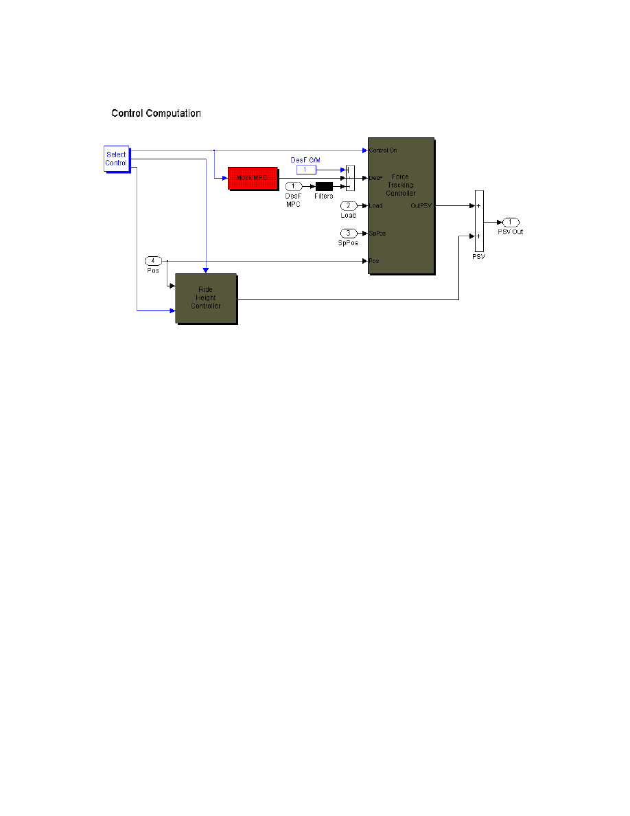
66

C.2.2 Control

Modules

Figure C.4: Simulink model of underneath the “Control Computation” block

An integer, set from Cockpit determines which primary actuator control scheme is

enabled by the “Select Control” block. The desired force for the force-tracking controller

is either generated by the “Mock MPC” or computed on the Alpha board by a high-level

controller.

Ride Height, PI Control Module

PI controller provides a means to ensure a stable chassis when the pump is on and there

are no road disturbances. From the LVDT we know the expansion of the actuator, x.

Given some desired expansion x

des

a proportional integral (PI) controller was designed

such that:

∫

−

+

−

=

)

(

)

(

x

x

K

x

x

K

V

des

I

des

p

spool

(C.1)

The gain set {K

p

= 150, K

I

= 50} was determined empirically to achieve a reasonable

response with moderate comfort to the passengers. The Simulink diagram of the control

code for the four actuators is shown below. Given this code, any desired position

trajectory, within the limits of the actuators, can be obtained.

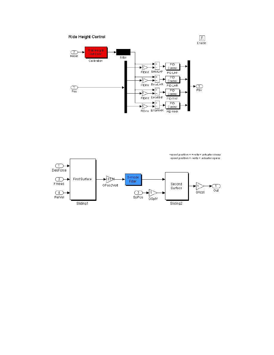
67

Figure C.5: Simulink model of the “Ride Height Controller”

Force Tracking Control Module

Figure C.6: Simulink model of the final version of the FTC for one actuator.

From the derivation of the controller in Chapter 2, there are two surfaces coupled by a

filter, as seen in Figure C.6. Controller surfaces were tuned independently. It is not

shown here but a scaled desired trajectory was passed directly to the second surface

during tuning. Furthermore, an open loop control signal could be sent directly to the

spool valve servo amplifier. This was important for collecting the data needed for

parameter estimation. Below is one incarnation of the ORD FTC first surface described

by equation (2.16).

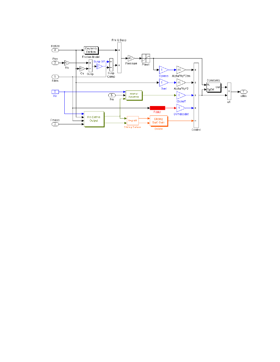
68

Figure C.7: Simulink model of a fully populated force surface for one actuator’s FTC

Notice the plethora of gain blocks. These blocks allow the respective terms to be

adjusted from Cockpit. The performance of the FTC is determined by the accuracy of the

parameters. The gain blocks allow real-time manipulation of the values.

C.2.3 Subsystem

Modules

Subsystem modules were computed on the Alpha board. In the code structure shown in

Figure C.8, there are three primary computations for the Alpha board: the MPC, the

preview buffer and the Kalman Filter (KF). The base sampling rate for the board is

10ms; this means the inputs and outputs are processed at 10ms. Due to processor

constraints the MPC is run at a 30ms sampling rate. To simplify the interactions, the KF,

HRF, and Sky Hook, are also run at 30ms. Transfer of data between tasks of different

sampling rates is done one of two ways:

1. Faster task (10ms) to slower task transitions: zero order hold

2. Slower task (“MPC Mod”) to faster task (output): data is written to a buffer.

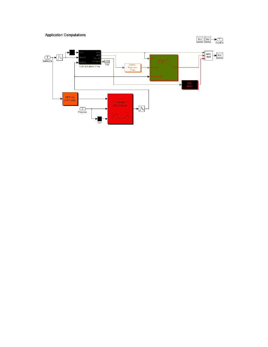
69

Figure C.8: Simulink model of “CPU Alpha”, notice inter-task data transfer methods

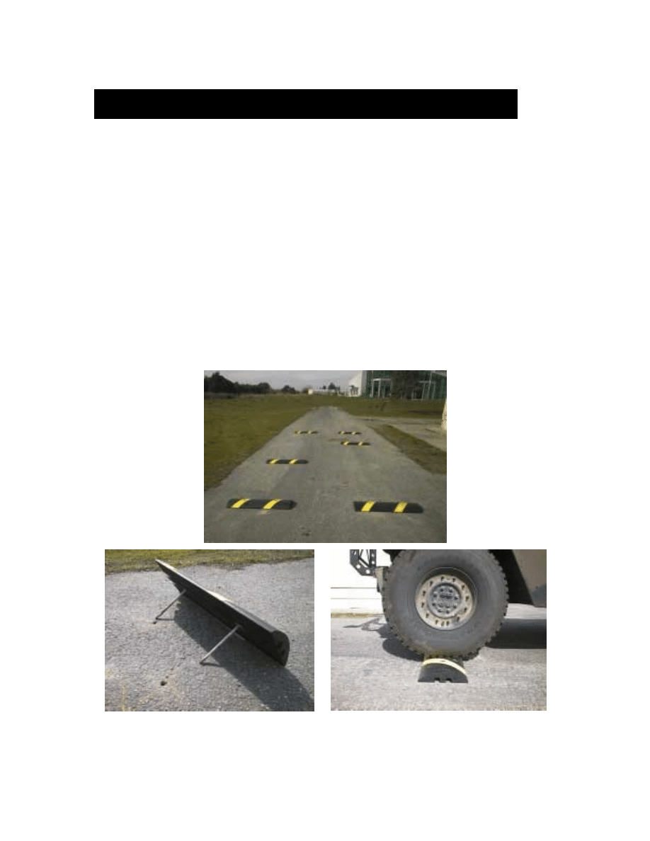
70

Appendix D - Test Track

The HMMWV is stored at the University of California’s Richmond Field Station (RFS)

in Richmond, CA. In addition to storage, RFS provides the local for testing. The

available testing paradigms are: 1. a custom test track, described below, 2. gravel roads,

3. dirt roads, and 4. off-road, grassy terrain.

For the test track we have opted for an asphalt, instead of a dirt, road surface to limit the

effects of weather, erosion, and wear. Six standard, hard rubber speed bumps,

manufactured by Scientific Developments Inc., are used. There are 10 possible

temporary locations for the bumps along the 32’ test region. Bump raisers are used to

increase the height of the bumps in 1.5” increments. Photos of the test track follow.

Figure D.1: Photographs of RFS active suspension test track

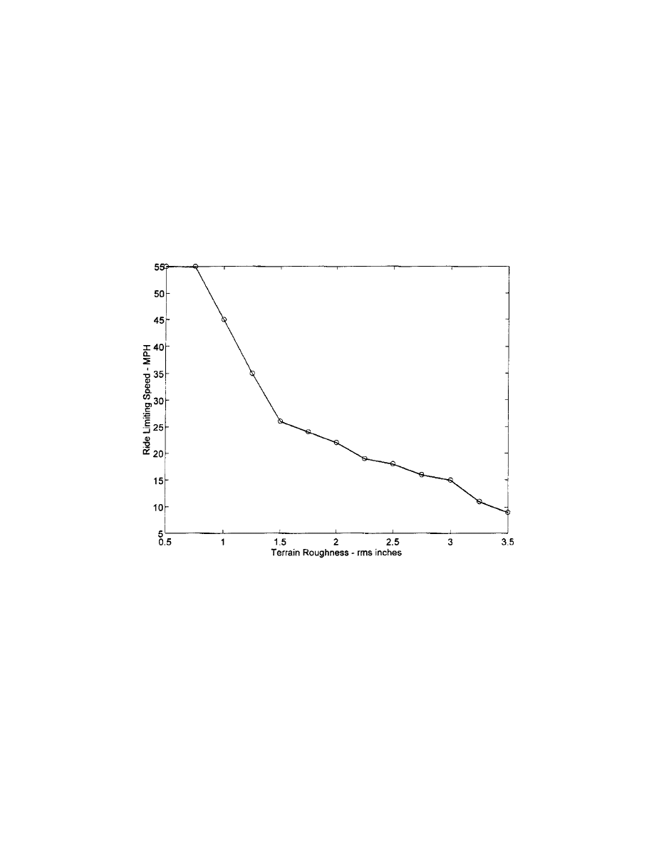
71

TARDEC has conducted extensive research on terrain roughness values and how they

relate to the human drivable speed for a given road. The maximum drivable speed is the

speed that the Cumulative Absorbed Power, see Section 3.4, reaches 6 Watts. Figure D.2

presents this information for a standard HMMWV. Although is has not yet been done, a

terrain roughness value will be computed for the test track profile. Perhaps some sections

of the dirt, gravel or off-road test tracks will be measured and converted as well. With

that information, a true valuation of the MPC results presented herein can be obtained.

Figure D.2: Plot of rate limiting speed for a given terrain roughness. 55mph is taken as the

maximum attainable HMMWV speed.

72

Appendix E - Glossary

Nomenclature

Piston area = 0.0044 m

2

Discharge coefficient = 0.7

Leakage coefficient =

2

/

em

im

C

C

+

= 15e-12

Suspension damping = 12000 Ns/m

Tire damping = 200 Ns/m

Actuator

force

Friction force = 120 N

Voltage to position conversion factor = 1481 V/m

Suspension spring stiffness = 240 kN/m

Tire spring stiffness = 1000 kN/m

Relative velocity, chassis → axle = 2.1

Sprung mass = 2800 kg

Un-sprung mass = 270 kg

Equivalent

mass

(

)

s

u

m

m

1

1

+

Supply pressure = 20684 kN/m

2

Pressure induced by load

Spool valve position

Bypass valve area

Input voltage command

Total volume of actuator cylinder chamber

Spool valve width = 0.008 m

Hydraulic coefficient =

t

V

/

4

β

= 2.273e9 N/m

5

Bulk modulus of hydraulic fluid

Specific gravity of hydraulic fluid = 3500

p

A

i

d

C

tm

C

s

c

t

c

A

F

f

F

k

s

m

eq

m

s

k

t

k

s

P

L

P

1

u

2

u

t

V

w

α

β

ρ

V

v

k

u

m

73

Acronyms

RHC

Ride

Height

Controller

FTC

Force

Tracking

Controller

ORD

Output Redefinition of FTC

SKY

Sky Hook Damping Controller

LQR

Linear

Quadratic

Regulator

FSLQ

Frequency Shaped Linear Quadratic Controller

VDC

Velocity

Damping

Controller

MPC

Model

Predictive

Controller

MPC

p

Model Predictive Controller with Preview

HRF

Human

Response

Filter

CAP

Cumulative

Absorbed

Power

HPR

Heave Pitch & Roll

pH

Preview Horizon for MPC

DOF

Degree

of

Freedom

LHF

Left/Right

Hand

Front/Rear

LVDT

Linear Variable Displacement Transducer

BASR

Berkeley Active Suspension Rig

HMMWV

High Mobility Multi-Purpose Wheeled Vehicle

UCB

The University of California at Berkeley

SSCI

Scientific Systems Company Inc.

SBIR

Small Business Innovative Research

TACOM

Tank Automotive & Armaments Command

TARDEC

Tank Automotive Research, Development Center