
Lectures at Stanford
Geometric scattering theory
Richard B. Melrose
Massachusetts Institute of Technology
CAMBRIDGE UNIVERSITY PRESS
Cambridge
New York
Port Chester
Melbourne
Sydney


Preface
These notes are based on lectures delivered at Stanford University in
January
1
1994 and then repeated at MIT in the Spring semester. I am
very grateful to the members of the Mathematics Department at Stan-
ford, and in particular Ralph Cohen, for the invitation and hospitality.
My especial thanks to those who attended the lectures and contributed
in one way or another. I am particularly pleased to acknowledge the
influence on my thinking of two of the members of the audience, Ralph
Phillips and Joe Keller. Rafe Mazzeo encouraged me to write up the lec-
tures, provided me with his own notes and, as if that were not enough,
made many helpful comments on the manuscript. I should also like to
extend my thanks to Sang Chin, Daniel Grieser, Andrew Hassell, Mark
Joshi, Olivier Lafitte, Eckhard Meinrenken, Edith Mooers and Andras
Vasy who attended the second hearing
2
of the lectures at MIT and to-
gether made many useful remarks; Andras Vasy was particularly helpful
in reading and correcting the notes as they dribbled out. I would also
like to thank Tanya Christiansen and Gunther Uhlmann for their assis-
tance and Lars H¨
ormander, Georgi Vodev and Maciej Zworski for their
comments on later versions of the manuscript.
3
It is my hope that these notes may serve as an introduction to an
active and growing area or research, although I fear they represent a
rather steep learning curve.
1
It was a horrible month in Cambridge I am told, very pleasant indeed in Palo Alto.
This footnote is an indication of things to come in the body of the notes. If you
can’t stand it, stop now!
2
Of course I had really wanted to do things in the other order but did not manage
to get my thoughts together in time.
3
Of course, I claim sole credit for all remaining errors.
iii

Contents
List of Illustrations
page 1
Introduction
2
1
Euclidean Laplacian
3
1.1
The Laplacian
3
1.2
Spectral resolution
4
1.3
Scattering matrix
6
1.4
Resolvent family
8
1.5
Limiting absorption principle
9
1.6
Analytic continuation
11
1.7
Asymptotic expansion
13
1.8
Radial compactification
15
2
Potential scattering on R
n
17
2.1
The resolvent of ∆ + V
17
2.2
Poles of the resolvent
20
2.3
Boundary pairing
21
2.4
Formal solutions
23
2.5
Unique continuation
23
2.6
Perturbed plane waves
24
2.7
Relative scattering matrix
24
2.8
Asymptotics of the resolvent
26
2.9
L
2
eigenfunctions
27
2.10 Zero energy states
27
2.11 Meromorphy of the scattering matrix
28
3
Inverse scattering
29
3.1
Radon transform
29
3.2
Wave group
32
3.3
Wave operators
35
3.4
Lax-Phillips transform
35
iv

Contents
v
3.5
Travelling waves
36
3.6
Near-forward scattering
38
3.7
Constant-energy inverse problem
39
3.8
Exponential solutions
41
3.9
Backscattering
42
4
Trace formulæ and scattering poles
44
4.1
Determinant and scattering phase
45
4.2
Poisson formula
47
4.3
Existence of poles
48
4.4
Lax-Phillips semigroup
49
4.5
Counting function
50
4.6
Pole-free regions
53
5
Obstacle scattering
54
5.1
Obstacles
55
5.2
Scattering operator
57
5.3
Reflected geodesics
58
5.4
Ray relation
61
5.5
Trapped rays
64
6
Scattering metrics
67
6.1
Manifolds with boundary
68
6.2
Hodge theorem
69
6.3
Pseudodifferential operators
70
6.4
Symbol calculus
73
6.5
Index theorem
76
6.6
Limiting absorption principle
77
6.7
Generalized eigenfunctions
78
6.8
Scattering matrix
79
6.9
Long-range potentials
81
6.10 Other theorems?
81
7
Cylindrical ends
82
7.1
b-geometry
83
7.2
Thresholds
85
7.3
Scattering matrix
87
7.4
Boundary expansions and pairing
88
7.5
Hodge theory
89
7.6
Atiyah-Patodi-Singer index theorem
90
7.7
b-Pseudodifferential operators
92
7.8
Trace formula and spectral asymptotics
93
7.9
Manifolds with corners
94

vi
Contents
8
Hyperbolic metrics
96
8.1
Warped products
96
8.2
Conformally compact manifolds
98
8.3
0-geometry and analysis
100
8.4
The Laplacian
102
8.5
Analytic continuation
104
8.6
Finite volume quotients
105
8.7
hc-geometry
105
8.8
Spectrum
106

List of Illustrations
1
The contours γ
+
(λ
′
) and γ
−
(λ
′
).
10
2
Analytic continuation of the resolvent for n odd.
12
3
Analytic continuation of the resolvent for n even.
13
4
Stereographic, or radial, compactification of R
n
.
15
5
Poles of the analytic continuation of R
V
(λ) (n odd)
22
6
The Lax-Phillips semigroup
49
7
Reflected geodesics.
59
8
Non-uniqueness of extension of reflected geodesics.
60
9
Two secret rooms
63
10
The compactified scattering cotangent bundle
75
11
Geodesic of a scattering metric.
80
12
Spectrum of the Laplacian of an exact b-metric
86
13
Geodesics for a conformally compact metric
104
1

Introduction
The lectures on which these notes are based were intended as an, es-
sentially non-technical, overview of scattering theory. The point of view
adopted throughout is that scattering theory provides a parametrization
of the continuous spectrum of an elliptic operator on a complete man-
ifold with uniform structure at infinity. The simple, and fundamental,
case of the Laplacian on Euclidean space is described in the first two lec-
tures to introduce the basic framework of scattering theory. In the next
three lectures various results on Euclidean scattering, and the methods
used to prove them, are outlined. In the last three lectures these ideas
are extended to non-Euclidean settings. This is an area of much cur-
rent research and my idea was to show how similar the Euclidian and the
less familiar cases are. Some of the interactions of scattering theory with
hyperbolic geometry, index theory and Hodge theory are also indicated.
I have made no attempt at completeness here but simply described
what time, and my own tastes, indicate. In particular there should be at
least three times as many references as there are. If I have offended by
omitting reference to important work, this should not be interpreted as
a deliberate slight! In writing up the lectures I have made extensive use
of footnotes to cover more subtle points, to clarify statements that were
felt to be obscure, by someone, and to make comments. These asides
can be freely ignored.
2

1
Euclidean Laplacian
1.1 The Laplacian
A fundamental aspect of scattering theory, and one to which I shall
give considerable emphasis, is the parametrization of the continuous
spectrum of differential operators, especially the Laplace operator. I
therefore want to begin these lectures with a discussion of the spectral
theory of the flat Laplacian on Euclidean space:
∆ = D
2
1
+ D
2
2
+ · · · + D
2
n
on R
n
, D
j
=
1
i
∂
∂z
j
(1.1)
where z
1
, . . . , z
n
are the standard coordinates. Notice that this is the
‘geometer’s
1
Laplacian’ whereas the ‘analyst’s Laplacian’ is −∆.
2
To a large extent below, except where it is really important, I shall
avoid functional analytic statements relating to the boundedness of op-
erators on Hilbert spaces. Thus I shall consider, at least initially, ∆ as
an operator on Schwartz’ space
3
of C
∞
functions which decrease rapidly
at infinity with all derivatives:
S(R
n
) =
u : R
n
−→ C ; sup
z∈
R
n
|z
α
D
β
u(z)| < ∞
.
(1.2)
1
Of course it depends on the sort of ‘geometer’ you know; this positive Laplacian
is the 0-form case of the Hodge Laplacian. Some geometers use the analysts’
convention.
2
The ‘scattering theorist’s Laplacian’ is either −i∆ or A =
0
Id
∆
0
. The reason
for considering A should become clearer in Section 3.2.
3
See [42], Definition 7.1.2. It is somewhat contradictory to be using S(R
n
), which
is a more subtle space topologically than are Hilbert spaces such as L
2
(R
n
); nev-
ertheless doing so avoids the discussion of unbounded operators. See also [103].
3

4
Euclidean Laplacian
The Fourier transform
b
f (ζ) =
Z
R
n
e
−iz·ζ
f(z)dz
(1.3)
is an endomorphism
4
of S(R
n
) with inverse
f(z) = (2π)
−n
Z
R
n
e
iz·ζ
b
f (ζ)dζ.
(1.4)
Since
5
d
D
j
f = ζ
j
b
f , conjugation by the Fourier transform reduces any
constant coefficient operator to multiplication by a function, in particu-
lar
c
∆f = |ζ|
2
b
f, ∀ f ∈ S(R
n
).
(1.5)
1.2 Spectral resolution
Using (1.5), and the inversion formula (1.4), the form of the spectral
resolution
6
of ∆ can be readily deduced. Introducing polar coordinates,
ζ = λω, λ = |ζ| in (1.4) gives
f(z) = (2π)
−n
∞
Z
0
Z
S
n−1
e
iλz·ω
λ
n−1
b
f (λω)dωdλ.
(1.6)
This can be rewritten as a decomposition of the identity operator:
Id =
∞
Z
0
E
0
(λ)dλ, E
0
(λ)f = (2π)
−n
Z
S
n−1
e
iλz·ω
λ
n−1
b
f (λω)dω.
(1.7)
4
See [42], Theorem 7.1.5.
5
See [42], Lemma 7.1.4.
6
See [98] for a discussion of the spectral theorem; it is not necessary to know this
result to proceed (in fact this admonition could be appended to many subsequent
comments.)
1.2 Spectral resolution
5
Here
7
E
0
(λ)dλ is a projection-valued measure
8
which gives the spectral
decomposition of the Laplacian
∆ =
∞
Z
0
λ
2
E
0
(λ)dλ.
(1.8)
The operator E
0
(λ) has range in the null space of ∆ − λ
2
; as follows
from the fact that the ‘plane waves’ Φ
0
(z, ω, λ) = exp(iλz · ω) are, for
ω ∈ S
n−1
, solutions of (∆ − λ
2
)Φ
0
= 0. It is convenient to decompose
E
0
(λ) as a product of two operators. Define
9
(Φ
0
(λ)g)(z) =
Z
S
n−1
Φ
0
(z, ω, λ)g(ω)dω, Φ
0
(z, ω, λ) = e
iλz·ω
.
(1.9)
Thus Φ
0
(λ) : C
∞
(S
n−1
) −→ S
′
(R
n
), the space of tempered distributions.
The formal adjoint operator is just
10
(Φ
∗
0
(λ)f)(ω) =
Z
R
n
Φ
0
(z, ω, −λ)f(z)dz, Φ
∗
0
(λ) : S(R
n
) −→ C
∞
(S
n−1
),
(1.10)
since Φ
0
(z, ω, −λ) = Φ
0
(z, ω, λ). Then the definition (1.7) becomes
E
0
(λ) = (2π)
−n
λ
n−1
Φ
0
(λ)Φ
∗
0
(λ), λ > 0.
(1.11)
Now, for fixed 0 6= λ ∈ R, Φ
∗
0
(λ) is surjective as a map (1.10).
11
Thus
to compute the range of E
0
(λ) it is only necessary to find the range of
Φ
0
(λ). In fact it is as large as could reasonably be expected.
7
λ is the ‘frequency’ of the wave e
iλz·ω
.
8
It is not the case that E
0
(λ) maps f ∈ S(R
n
) into S(R
n
); the form of the range
is discussed below. One might therefore wonder on what space this is supposed
to be a projection! One way to explain this is in terms of the average of the
E
0
(λ). If q ∈ C
∞
c
((0, ∞)) is a smooth function of compact support set E
0
(q)f =
∞
R
0
q(λ)E
0
(λ)f dλ. Then E
0
(q) : S(R
n
) −→ S(R
n
) and for any two functions q,
q
′
∈ C
∞
c
((0, ∞)) it is always the case that E
0
(q) ◦ E
0
(q
′
) = E
0
′
).
9
As a general convention I use the same notation for the operator and its Schwartz
kernel. Of course this is a possible source of confusion and error, in particular one
has to be careful as to which variables are regarded as parameters and what is
the splitting into ‘incoming’ and ‘outgoing’ variables. Nevertheless I feel that this
danger is outweighed by the consequent reduction in the number of symbols.
10
So one can reasonably say that Φ
∗
0
(z, ω, λ) = Φ
†
(z, ω, λ), where the † tells one to
reverse the order of the variables and so get the transpose.
11
As follows from the properties of the Fourier transform, since any smooth function
on the sphere |ζ| = λ > 0 is the restriction of an element of S(R
n
).
6
Euclidean Laplacian
Lemma 1.1
12
For 0 6= λ ∈ R the range of Φ
0
(λ), acting on distributions
on S
n−1
, is the null space of ∆ − λ
2
acting on the space, S
′
(R
n
), of
tempered distributions on R
n
.
1.3 Scattering matrix
Thus all the solutions of (∆ − λ
2
)u = 0 with u ‘of polynomial growth’
are superpositions of the elementary plane wave solutions Φ
0
(z, ω, λ) =
e
iλz·ω
where ω ∈ S
n−1
. The plane waves give a ‘continuous
13
parametriz-
ation’ of the eigenspace; there is a related ‘functional parametrization’
of it which is also important.
If g in (1.9) is taken to be smooth then the principle of stationary
phase
14
can be used to understand the behaviour of Φ
0
(λ)g as |z| → ∞.
Writing z = |z|θ, θ = z/|z| ∈ S
n−1
gives
Φ
0
(λ)g(|z|θ) =
Z
S
n−1
e
i|z|λθ·ω
g(ω)dω.
(1.12)
The phase function θ · ω as a function of ω ∈ S
n−1
is stationary, i.e. has
vanishing gradient, exactly at the two points ω = ±θ. Since the Hessian
at these points is non-degenerate
15
the stationary phase lemma gives a
complete asymptotic expansion
16
Φ
0
(λ)g(|z|θ) ∼ e
iλ|z|
(λ|z|)
−
1
2
(n−1)
e
−
1
4
π(n−1)i
(2π)
1
2
(n−1)
X
j≥0
|z|
−j
h
+
j
(θ)
+e
−iλ|z|
(λ|z|)
−
1
2
(n−1)
e
1
4
π(n−1)i
(2π)
1
2
(n−1)
X
j≥0
|z|
−j
h
−
j
(θ), λ > 0,
(1.13)
12
This is simple to prove using the structure theory of distributions. Namely if
(∆ − λ
2
)u = 0 with u ∈ S
′
(R
n
), the dual space to S(R
n
), then the Fourier
transform
b
u(ζ) satisfies (|ζ|
2
− λ
2
)
b
u(ζ) = 0. If λ 6= 0 it follows that, written in
terms of polar coordinates z = rθ,
b
u = δ(r − |λ|)g
′
(θ) for some distribution on
the sphere g
′
∈ C
−∞
(S
n−1
). The inverse Fourier transform then shows that u is
Φ
0
(λ)g for g = (2π)
−n
λ
n−1
g
′
.
13
Really this is a smooth parametrization. One view of scattering theory is that it
describes the smoothness of the spectrum of appropriate operators.
14
By a ‘principle’ here is meant an old theorem which has had many manifestations.
For a precise statement of an appropriate version see [42], Section 7.7.
15
That is, ω · θ is a Morse function on the sphere.
16
This means that for any integer N the difference between the left side and the par-
tial sum over j ≤ N on the right side is bounded, in |z| ≥ 1, by C|z|
−N −1−
1
2
(n−1)
for some constant C. The power here is just the size of the first term dropped from
the sums. In fact the same is true after any number of formal derivatives with
respect to θ, or r = |z|, are taken (on both sides of course).

1.3 Scattering matrix
7
in which h
±
0
(θ) = g(±θ) and the h
±
j
for j ≥ 1 are all given by polynomials
in the Laplacian on the sphere applied to g(±θ).
Lemma 1.2
17
For each λ > 0 and each h ∈ C
∞
(S
n−1
) there is a unique
solution to (∆ − λ
2
)u = 0 such that as |z| → ∞
18
u(|z|θ) = e
iλ|z|
|z|
−
1
2
(n−1)
h(θ)
+e
−iλ|z|
|z|
−
1
2
(n−1)
h
′
(θ) + O
|z|
−
1
2
(n+1)
(1.15)
where h
′
∈ C
∞
(S
n−1
), and necessarily
19
h
′
(θ) = A
0
h(θ) = i
n−1
h(−θ).
(1.16)
This parametrizes the generalized eigenspace with eigenvalue λ
2
by the
distributions
20
on the sphere at infinity. Notice that ±λ give different
parametrizations of the same space, one in terms of h and the other
in terms of h
′
. The relationship between these two parametrizations
is given by (1.16) and this operator, mapping h(θ) to i
(n−1)
h(−θ), is
the ‘absolute scattering matrix’ for Euclidean space. It is a unitary
isomorphism of C
∞
(S
n−1
).
21
There are various stronger forms of this lemma, as far as the unique-
ness part is concerned. One particularly convenient one arises from the
17
The existence part follows from (1.13). To prove the uniqueness it is only necessary
to prove a variant of (1.13) for Φ
0
(λ)g where g ∈ C
−∞
(S
n−1
) is a distribution.
This can be done by using the same formula, (1.12), integrated against a test
function in C
∞
(S
n−1
). The stationary phase expansion in the θ variable shows
that
Φ
0
(λ)g(|z|θ) = e
iλ|z|
(λ|z|)
−
1
2
(n−1)
e
−
1
4
π(n−1)i
(2π)
1
2
(n−1)
g(θ)
+e
−iλ|z|
(λ|z|)
−
1
2
(n−1)
e
1
4
π(n−1)i
(2π)
1
2
(n−1)
g(−θ) + u
′
(1.14)
where u
′
∈ H
−∞
(R
n
) is in the union of all the standard Sobolev spaces; moreover
g is determined by this expansion since neither the first two terms separately, not
their sum, can be in H
−∞
(R
n
) unless g = 0. Given two solutions of the form
(1.15), the difference is a solution with h = 0. From Lemma 1.1 it follows that
this difference is of the form Φ
0
(λ)g for some g. The uniqueness of the expansion
(1.14) then shows that g = 0. Some further comments on the uniqueness will be
made in Lecture 2.
18
The ‘big Oh’ notation here means that the difference of the left and right sides is
bounded by C|z|
−
1
2
(n+1)
in |z| ≥ 1 for some constant C.
19
As defined here the operator A
0
is independent of λ. However, there is also a
unique solution on the form (1.15) for λ < 0. If n is odd, the resulting operator
mapping h to h
′
is the same. If n is even it is not, rather it is −A
0
.
20
I mean here that the map h 7→ u ∈ S
′
(R
n
) extends by continuity to all
h ∈ C
−∞
(S
n−1
) and then gives a parametrization of all the tempered general-
ized eigenfunctions.
21
If n is odd it is an involution, i.e. A
0
◦ A
0
= Id, whereas if n is even it is a fourth
root of unity in the sense that A
4
0
= Id . This sort of behaviour, depending on the
parity of the dimension, can be seen much more strongly in 1.6.

8
Euclidean Laplacian
observation that the function |z|
−
1
2
(n−1)
is locally square-integrable near
0 and that |z|
−
1
2
(n+1)
is square-integrable near |z| = ∞.
22
Thus (1.15)
implies that
u(|z|θ) =e
iλ|z|
|z|
−
1
2
(n−1)
h(θ)
+e
−iλ|z|
|z|
−
1
2
(n−1)
h
′
(θ) + u
′
, u
′
∈ L
2
(R
n
).
(1.17)
Conversely, for a solution to (∆ −λ
2
)u = 0, this implies (1.15) and hence
(1.13).
Notice from (1.13) that the map C
∞
(S
n−1
) 7−→ S
′
(R
n
) which gives
the unique solution of the form (1.15) is
u(z) = P
0
(λ)h = λ
1
2
(n−1)
e
1
4
π(n−1)i
(2π)
−
1
2
(n−1)
Φ
0
(λ)h, λ > 0.
(1.18)
It would be reasonable to call the operator P
0
(λ) the ‘Poisson operator’
for the ‘boundary problem’ which seeks the solution to (∆ − λ
2
)u = 0
of the form (1.15) with h given.
23
1.4 Resolvent family
I should pay at least lip service to the fundamental fact that the Laplac-
ian is an essentially self-adjoint operator.
24
In particular the inverse of
the operator ∆ −σ, for σ ∈ C \ R is a bounded operator on L
2
(R
n
). This
is certainly true and much more can be seen, namely that this operator
can be obtained in terms of the Fourier transform:
(∆ − σ)
−1
f(z) = (2π)
−n
Z
R
n
e
iz·ζ
(|ζ|
2
− σ)
−1
b
f(ζ)dζ
(1.19)
whenever σ ∈ C \ [0, ∞).
25
Since the spectrum
26
is confined to the positive real axis it is conve-
nient to introduce λ
2
= σ as a modified spectral parameter. There are
two obvious normalizations of the choice of λ; I shall choose the ‘physical
22
That is, the function is square-integrable on the complement of any ball of positive
radius around the origin.
23
The mapping properties of an operator such as P
0
(λ) can be understood in terms
of Besov spaces, see [43].
24
If you want to know what this means see [98].
25
Since then |ζ|
2
− σ has no zeroes for ζ ∈ R
n
.
26
The spectrum is the singular set of the resolvent family.

1.5 Limiting absorption principle
9
domain’ to be the set
27
P = {λ ∈ C ; Im λ < 0}.
(1.20)
Then define
R
0
(λ) = (∆ − λ
2
)
−1
, λ ∈ P, i.e. Im λ < 0.
(1.21)
I will usually refer to this, slightly incorrectly,
28
as ‘the resolvent.’ From
(1.19) it follows that
R
0
(λ) : S(R
n
) −→ S(R
n
) for Im λ < 0.
(1.22)
It is the unique operator with this property such that (∆ −λ
2
)◦R
0
(λ) =
Id on S(R
n
).
1.5 Limiting absorption principle
The resolvent of the Laplacian can be written as an integral operator:
R
0
(λ)f(z) =
Z
R
n
R
0
(λ, z, z
′
)f(z
′
)dz
′
,
R
0
(λ, z, z
′
) = (2π)
−n
Z
R
n
e
i(z−z
′
)·ζ
dζ
(|ζ|
2
− λ
2
)
.
(1.23)
The integral here is not absolutely convergent.
29
To avoid worrying
about this
30
I shall consider instead the kth power of the resolvent,
where for k >
1
2
n the corresponding integral is absolutely convergent
R
k
0
(λ, z, z
′
) = (2π)
−n
Z
R
n
e
i(z−z
′
)·ζ
dζ
(|ζ|
2
− λ
2
)
k
, Im λ < 0.
(1.27)
27
In the lectures themselves I used the opposite convention, that Im λ > 0 in the
physical domain, I regretted it then . . . . I hope that all the sign errors have been
eliminated, but I am not too confident.
28
In that the resolvent is (∆ − σ)
−1
.
29
It is relatively straightforward to compute the form of these kernels ‘explicitly;’
the result (as with almost everything else) is simpler in the odd-dimensional case
than the even-dimensional one. If n = 1 then
R
0
(λ, z, z
′
) = λ
−1
exp(−iλ|z − z
′
|).
(1.24)
If n ≥ 3 is odd then there is a polynomial, q
n
, of degree n − 3 in one variable such
that
R
0
(λ; z, z
′
) = |z − z
′
|
−n+2
q
n
(λ|z − z
′
|) exp(iλ|z − z
′
|).
(1.25)
For n ≥ 2 even
R
0
(λ; z, z
′
) =
1
4i
λ
2π|z − z
′
|
1
2
n−1
Ha
(1)
1
2
n−1
(λ|z − z
′
|)
(1.26)
where Ha
(1)
j
(z) is a Hankel function.
30
Not that it is a serious problem.
10
Euclidean Laplacian
......
.....
......
.............
..........
.....
...........
..
...........
.
.
....................
.
.
.
.
.
.
.
.
.
.
.
.
.
.
.
.
.
.
.
.
.
.
.
.
.
.
.
.
.
.
.
.
.
.
.
.
.
.
.
.
.
.
.
.
.
.
.
.
.
.
.
..............
.
.
.
.
.
.
.
.
.
.
.
.
.
.
.
.
.
.
.
.
.
.
.
.
.
....
....
..
..
.
.
.
.
.
.
.
.
.
.
.
.
.
.
.
.
.
.
.
.
.
.
.
.
.
.
.
.
.
.
.
.
.
.
.
.
...
.
•
λ
′
•
λ
′
− iǫ
Im ρ
Re ρ
γ
+
(λ
′
)
......
......
......
......
...............
..........
....
..
..........
..........
....
............................
.
.
.
.
.
.
.
.
.
.
.
.
.
.
.
.
.
.
.
.
.
.
.
.
.
.
.
.
.
.
.
.
.
.
.
.
.
.
.
.
.
.
.
.
.
.
.
.
.
.
.
..............
.
.
.
.
.
.
.
.
.
.
.
.
.
.
.
.
.
.
.
.
.
.
.
.
.
...........
..
.............
............. .............
........
.....
......
......
.
•
λ
′
•
λ
′
+ iǫ
Im ρ
Re ρ
γ
−
(λ
′
)
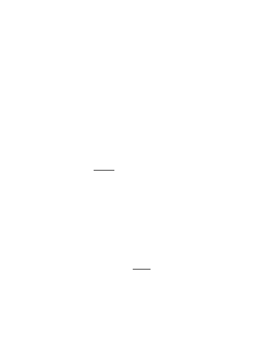
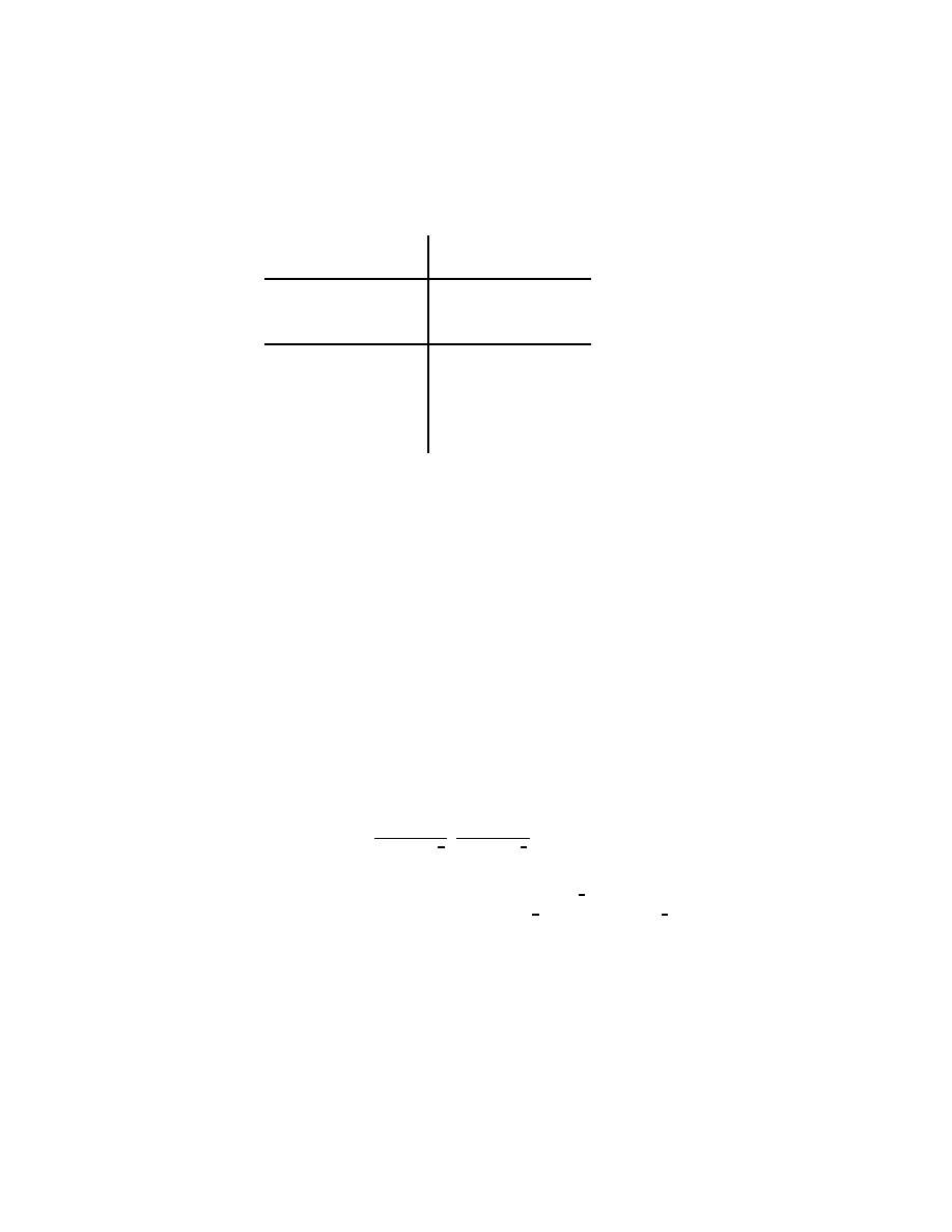
Fig. 1. The contours γ
+
(λ
′
) and γ
−
(λ
′
).
I am especially interested in what happens as Im λ ↑ 0 and the spectral
parameter σ = λ
2
approaches [0, ∞). Introducing polar coordinates in
ζ, as in (1.7), but now writing ζ = ρω, gives
R
k
0
(λ, z, z
′
) = (2π)
−n
Z
S
n−1
∞
Z
0
e
iρ(z−z
′
)·ω
ρ
n−1
dρ
(ρ
2
− λ
2
)
k
dω.
(1.28)
The integrand is holomorphic in ρ away from ρ = ±λ, where there is a
pole. If λ = λ
′
− iǫ with λ
′
> 0 and ǫ > 0 and small, then Cauchy’s
theorem can be used to move the contour in (1.28) to γ
+
(λ
′
) as in
Figure 1:
R
k
0
(λ, z, z
′
) = (2π)
−n
Z
S
n−1
Z
γ
+
(λ
′
)
e
iρ(z−z
′
)·ω
ρ
n−1
dρ
(ρ
2
− λ
2
)
k
dω, λ = λ
′
− iǫ.
(1.29)
Now the limit as ǫ ↓ 0 in (1.29) is not singular, provided λ
′
> 0. If
λ = −λ
′
− iǫ where λ
′
is still positive then in place of (1.29)
R
k
0
(λ, z, z
′
) = (2π)
−n
Z
S
n−1
Z
γ
−
(λ
′
)
e
iρ(z−z
′
)·ω
ρ
n−1
dρ
(ρ
2
− λ
2
)
k
dω,
λ = −λ
′
− iǫ,
(1.30)

1.6 Analytic continuation
11
with γ
−
(λ
′
) the contour going ‘the other way’ around λ
′
. Again the limit
as ǫ ↓ 0 can be taken. Since the two limiting points ±λ
′
correspond to
the same point σ = (λ
′
)
2
in the spectrum it is natural to consider the
difference:
R
k
0
(λ, z, z
′
) − R
k
0
( − λ, z, z
′
) =
(2π)
−n
Z
S
n−1
Z
γ
+
(λ)−γ
−
(λ)
e
iρ(z−z
′
)·ω
ρ
n−1
dρ
(ρ
2
− λ
2
)
k
dω, λ > 0.
(1.31)
The difference of the two contours is homotopic to a clockwise circle of
small radius around the single point λ, so Cauchy’s theorem can be used
to evaluate the integral as a residue. Using the identity (∆ − λ
2
)
j
R
k
0
=
R
k−j
0
(λ) for k > j
R
0
(λ; z, z
′
)−R
0
(−λ; z, z
′
)
=
1
2i
(2π)
−(n−1)
λ
n−2
Z
S
n−1
e
iλ(z−z
′
)·ω
dω, λ > 0.
(1.32)
This is the limiting absorption principle or it can be called, perhaps
more correctly, Stone’s theorem.
31
1.6 Analytic continuation
Formulæ (1.29) and (1.30) make sense for ǫ small compared to the radius
of the circular part of the contour (and hence with respect to λ
′
), of
either sign. This shows that R
0
(λ, z, z
′
) can be continued analytically,
as a function of λ, through the real axis, at least away from 0. Indeed if
I define M (λ), in terms of right side of (1.32):
M (λ, z, z
′
) =
1
2i
(2π)
−(n−1)
Z
S
n−1
e
iλ(z−z
′
)·ω
dω, λ > 0,
(1.34)
then observe that M (λ; z, z
′
) extends to be an entire function of λ ∈ C .
I shall denote, temporarily, by e
R
0
(λ) the function
32
defined by analytic
continuation of R
0
(λ) across (0, ∞). Thus e
R
0
(λ) = R
0
(λ) in Im λ < 0,
31
Which can be stated briefly in the present context as the assertion that the spectral
resolution can be obtained from the difference of the limits, from above and below,
of the resolvent family on the spectrum. Notice that by inserting the Fourier
transform in (1.7) it follows that
E
0
(λ) =
λi
π
(R
0
(λ) − R
0
(−λ)) , λ ∈ (0, ∞).
(1.33)
32
Really to be thought of as an operator.
12
Euclidean Laplacian
...............
.
.
.
.
.
.
.
.
.
.
.
.
.
.
.
.
.
.
.
.
.
.
.
.
.
.
.
.
.
.
.
.
.
.
.
.
.
.
.
.
.
.
.
.
.
.
.
.
.
.
.
.....
.....
.....
.............
..........
.....
...........
..........
.....
. . . . . . . . . . . . . . . . . . . . . . . . . . . . . . . . . .
. . . . . . . . . . . . . . . . . . . . . . . . . . . . . . . . . . .
. . . . . . . . . . . . . . . . . . . . . . . . . . . . . . . . . .
. . . . . . . . . . . . . . . . . . . . . . . . . . . . . . . . . . .
. . . . . . . . . . . . . . . . . . . . . . . . . . . . . . . . . .
. . . . . . . . . . . . . . . . . . . . . . . . . . . . . . . . . . .
. . . . . . . . . . . . . . . . . . . . . . . . . . . . . . . . . .
. . . . . . . . . . . . . . . . . . . . . . . . . . . . . . . . . . .
. . . . . . . . . . . . . . . . . . . . . . . . . . . . . . . . . .
. . . . . . . . . . . . . . . . . . . . . . . . . . . . . . . . . . .
. . . . . . . . . . . . . . . . . . . . . . . . . . . . . . . . . .
. . . . . . . . . . . . . . . . . . . . . . . . . . . . . . . . . . .
. . . . . . . . . . . . . . . . . . . . . . . . . . . . . . . . . .
. . . . . . . . . . . . . . . . . . . . . . . . . . . . . . . . . . .
. . . . . . . . . . . . . . . . . . . . . . . . . . . . . . . . . .
. . . . . . . . . . . . . . . . . . . . . . . . . . . . . . . . . . .
. . . . . . . . . . . . . . . . . . . . . . . . . . . . . . . . . .
. . . . . . . . . . . . . . . . . . . . . . . . . . . . . . . . . . .
. . . . . . . . . . . . . . . . . . . . . . . . . . . . . . . . . .
. . . . . . . . . . . . . . . . . . . . . . . . . . . . . . . . . . .
. . . . . . . . . . . . . . . . . . . . . . . . . . . . . . . . . .
. . . . . . . . . . . . . . . . . . . . . . . . . . . . . . . . . . .
. . . . . . . . . . . . . . . . . . . . . . . . . . . . . . . . . .
0
Im λ
Re λ
P
σ=λ
2
−→
.................
.
.
.
.
.
.
.
.
.
.
.
.
.
.
.
.
.
.
.
.
.
.
.
.
.
.
.
.
.
.
.
.
.
.
.
.
.
.
.
.
.
.
.
.
.
.
.
.
.
.
.
.....
......
.....
...............
..........
....
.
...........
..
...........
.
0
Im σ
Re σ
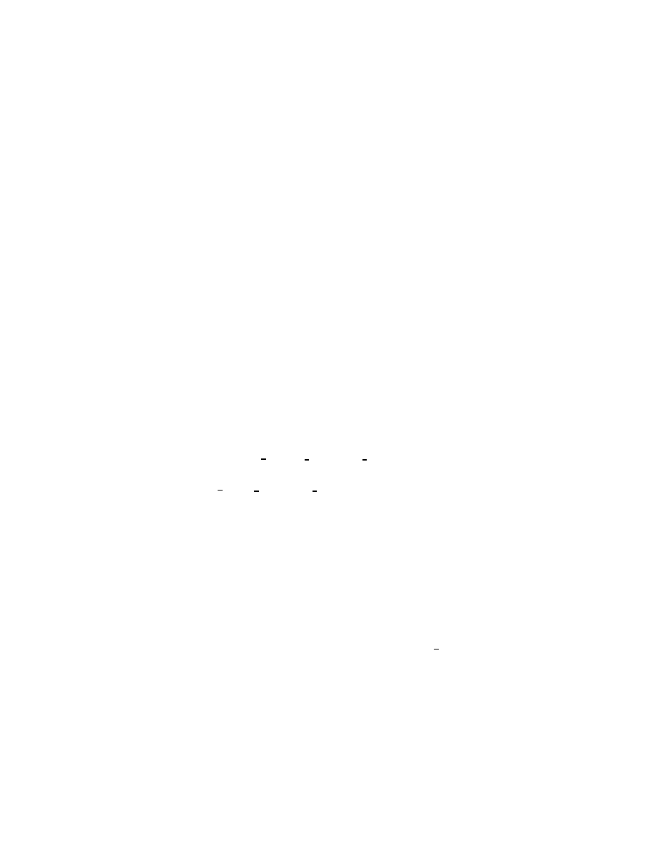
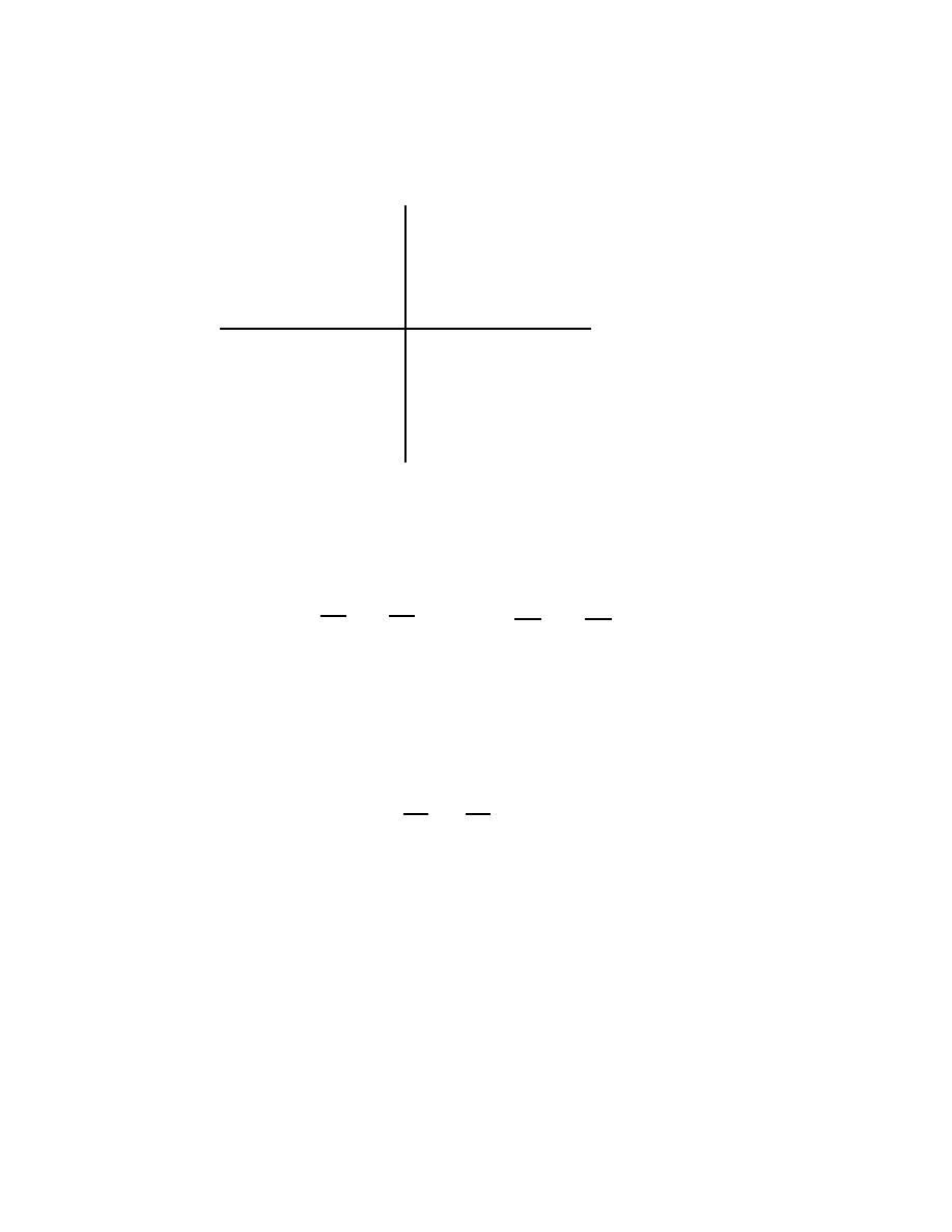
Fig. 2. Analytic continuation of the resolvent for n odd.
but e
R
0
(λ) is also defined near the positive real axis. From (1.32) it
follows that, for λ near the positive real axis with Im λ > 0,
e
R
0
(λ) = R
0
(−λ) + λ
n−2
M (λ).
(1.35)
Thus in fact e
R
0
(λ) extends to be holomorphic for all Im λ > 0 as well as
near (0, ∞) and in Im λ < 0, i.e. e
R
0
(λ) is holomorphic in C \ (−∞, 0].
Using the antipodal map in the sphere it follows from (1.34) that
M (−λ) = M(λ).
(1.36)
Applying (1.35) twice gives
lim
ǫ↓0
e
R
0
(−λ
′
+ iǫ)− lim
ǫ↑0
e
R
0
(−λ
′
+ iǫ)
=
(
0
n odd
2(λ
′
)
n−2
M (λ
′
)
n even
λ
′
> 0,
(1.37)
This shows the basic difference between the odd- and even-dimensional
cases. For odd n ≥ 3, the resolvent kernel is locally integrable in z, z
′
and
entire
33
as a function of λ; for n = 1 it is meromorphic in λ with a simple
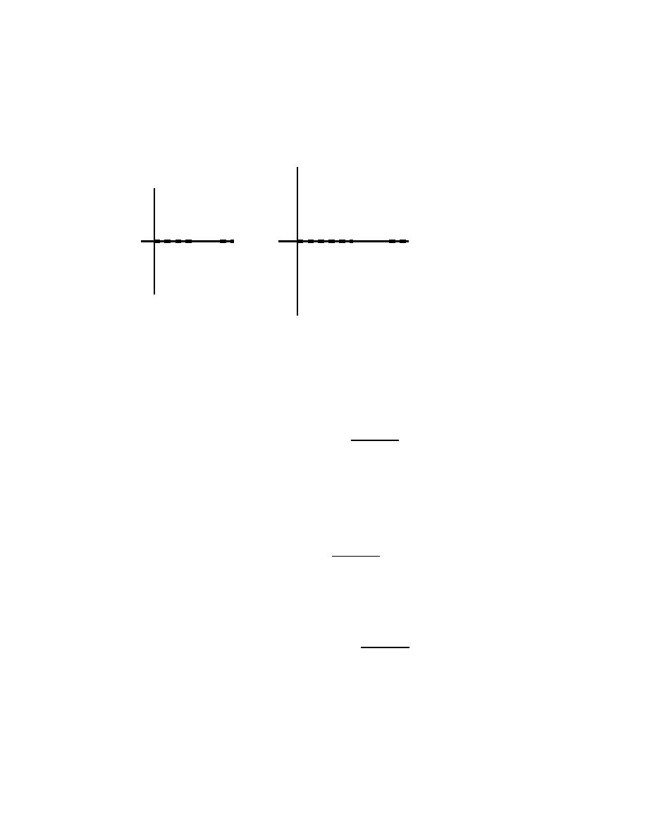
pole at 0. In the even-dimensional case a similar result is valid, except
that the kernel only extends to be entire on the logarithmic covering of
the complex plane, Λ, i.e. as a function of the variable log λ.
34
Thus if
R
♭
0
(τ ) = R
0
(λ) the ‘physical domain’ for R
♭
0
(τ ) can be taken as {τ ∈
R
× i(−π, 0) ⊂ C } and then R
♭
0
(τ ) extends to be entire on the τ -plane
33
It follows from (1.23) that there is neither an essential singularity, nor a pole, at
λ = 0.
34
In the even dimensional case the behaviour as λ → 0 can also be analyzed; in fact
R
0
(λ) = R
′
0
(λ) + M (λ)λ
n−2
log λ
(1.38)
where R
′
0
(λ) is entire.

1.7 Asymptotic expansion
13
...............
.
.
.
.
.
.
.
.
.
.
.
.
.
.
.
.
.
.
.
.
.
.
.
.
.
.
.
.
.
.
.
.
.
.
.
.
.
.
.
.
.
.
.
.
.
.
.
.
.
.
.
.....
.....
.....
.............
..........
.....
.
.
..
..
..........
..........
. . . . . . . . . . . . . . . . . . . . . . . . . . . . . . . . . .
. . . . . . . . . . . . . . . . . . . . . . . . . . . . . . . . . . .
. . . . . . . . . . . . . . . . . . . . . . . . . . . . . . . . . .
. . . . . . . . . . . . . . . . . . . . . . . . . . . . . . . . . . .
. . . . . . . . . . . . . . . . . . . . . . . . . . . . . . . . . .
. . . . . . . . . . . . . . . . . . . . . . . . . . . . . . . . . . .
. . . . . . . . . . . . . . . . . . . . . . . . . . . . . . . . . .
. . . . . . . . . . . . . . . . . . . . . . . . . . . . . . . . . . .
. . . . . . . . . . . . . . . . . . . . . . . . . . . . . . . . . .
. . . . . . . . . . . . . . . . . . . . . . . . . . . . . . . . . . .
. . . . . . . . . . . . . . . . . . . . . . . . . . . . . . . . . .
−iπ
0
Im τ
Re τ
P
σ=e
2
τ
−→
.................
.
.
.
.
.
.
.
.
.
.
.
.
.
.
.
.
.
.
.
.
.
.
.
.
.
.
.
.
.
.
.
.
.
.
.
.
.
.
.
.
.
.
.
.
.
.
.
.
.
.
.
.....
......
.....
...............
..........
....
.
.
..
..........
...........
.
0
Im σ
Re σ
Fig. 3. Analytic continuation of the resolvent for n even.
and has the special property that under the transformation τ 7→ τ +πi,
35
which corresponds to the shift from one preimage of the point λ = e
τ
to
another, it transforms by
R
♭
0
(τ + πi) = R
♭
0
(τ ) + e
(n−2)τ
M (e
τ
)
(1.39)
where M (λ) is the entire function of λ given by (1.34).
36
In either case
I shall denote the analytic continuation again by R
0
(λ), even though in
the even-dimensional case it is a function on Λ.
1.7 Asymptotic expansion
The expansion, (1.15), for elements of the null space of ∆ − λ
2
can be
extended to elements of the ‘near null space.’ More precisely
Proposition 1.1
If λ ∈ P ∪ (R\ {0})
37
then for each f ∈ C
∞
c
(R
n
)
38
(R
0
(λ)) f(|z|θ) ∼ e
−iλ|z|
|z|
−
1
2
(n−1)
∞
X
j=0
|z|
−j
h
j
(θ) as |z| → ∞,
(1.41)
35
This is the ‘deck-transformation’ for the covering of the λ-plane by the τ -plane.
36
Note that M (λ) can be expressed, for real λ > 0, as
M (λ) =
1
2i
(2π)
−(n−1)
Φ
0
(λ)Φ
∗
0
(λ).
(1.40)
Indeed this follows directly from (1.34) and (1.9), or (1.33).
37
Thus, Im λ ≤ 0 and λ 6= 0.
38
For real λ this result remains true for f ∈ S(R
n
), although the proof is a little
more involved.

14
Euclidean Laplacian
with h
j
∈ C
∞
(S
n−1
) and where
39
h
0
(θ) =
1
2iλ
P
†
0
(λ)f =
1
2i
(2π)
−
1
2
(n+1)
λ
1
2
(n−3)
e
1
4
π(n−1)i
b
f (−λθ), λ > 0.
(1.42)
This result can be proved using methods similar to those discussed in
Section 1.5.
40
If λ > 0 then only the first term in (1.41) is not square-
integrable near infinity. The solution u = R
0
(λ)f to (∆ − λ
2
)u = f is
then distinguished by the Sommerfeld radiation condition:
(
∂
∂r
+ iλ)u(rθ) ∈ L
2
(R
n
).
(1.46)
39
Here P
†
0
(λ) is the transpose of the operator P
0
(λ) in (1.18), so has the same kernel
but with the variables reversed in order.
40
I shall only discuss the proof for real λ. Consider R
0
(λ) which I have defined
as the limit of the resolvent from the physical region. Choose a cut-off function
φ ∈ C
∞
c
(R) which is 1 in an open neighbourhood of 1 and vanishes identically near
0. Then, for Im λ < 0,
R
0
(λ)f (z) = u
1
(z) + u
2
(z),
b
u
1
(ζ) = φ(
|ζ|
|λ|
)(|ζ|
2
− λ
2
)
−1
b
f (ζ).
(1.43)
Here, u
2
∈ S(R
n
) so it remains to analyze the behaviour of u
1
. Now fix θ = z/|z|
and consider another cut-off function on the sphere, ψ
0
∈ C
∞
(S
n−1
) such that
ψ
0
(ω) is identically equal to 1 in a neighbourhood of the equator ω · θ = 0 and
with ψ
0
(ω) vanishing identically in neighbourhoods of both ω = θ and ω = −θ.
Let 1 = ψ
0
+ ψ
+
+ ψ
−
be the resulting partition of unity with ψ
±
supported in
±θ · ω ≥ 0. Writing u
1
as the inverse Fourier transform of its Fourier transform,
introducing polar coordinates ζ = ρω and inserting this partition of unity gives
u
1
(z) = v
0
(z) + v
+
(z) + v
−
(z) where
v
t
= (2π)
−n
∞
Z
0
Z
S n−1
e
i|z|ρω·θ
ψ
t
(ω)(ρ
2
− λ
2
)
−1
ρ
n−1
φ
ρ
|λ|
b
f (ρω)dωdρ.
(1.44)
Of the three terms in (1.44) the only non-trivial one, asymptotically, is v
−
, since
v
0
, v
+
∈ S(R
n
) uniformly for Im λ ≤ 0 (but near a fixed non-zero real value λ
′
.)
For v
0
this follows by integration by parts in ω, using the fact that d
ω
(ω · θ) 6= 0
on the support of ψ
0
. For v
+
the ρ-integral can be deformed into the complex, as
γ
+
(λ
′
), using the fact that the integrand is analytic in ρ in a neighbourhood of
the deformed part. Similarly the ρ integral for v
−
can be deformed to a contour
integral over γ
−
(λ
′
) except that the pole at ρ = λ is encountered during the
deformation. Thus
R
0
(λ)f (|z|θ) =
1
2
(2π)
−n
λ
n−2
Z
S n−1
e
iλ|z|ω·θ
ψ
−
(ω)
b
f(λω)dω + w, w ∈ S(R
n
).
(1.45)
The asymptotic expansion then follows from the principle of stationary phase,
much as in (1.13).
1.8 Radial compactification
15
............................
.
.
.
.
.
.
.
.
.
.
.
.
.
.
.
.
.
.
.
.
.
.
.
.
.
.
.
.
.
.
.
.
.
.
.
.
.
.
.
.
.
.
.
.
.
.
.
.
.
.
.
......
......
......
......
...............
..........
....
.
...........
.
..........
..
.
......
..
.....
.
....
....
..
...
..
..
..
..
..
..
.
..
..
.
..
.
.
..
.
.
.
..
.
.
.
.
.
.
..
.
.
.
.
.
.
.
.
.
.
.
.
.
.
.
.
.
.
.
.
.
.
.
.
.
.
.
.
.
.
.
.
.
.
.
.
.
.
.
.
.
.
.
.
.
.
.
.
.
.
.
.
.
.
.
.
.
.
.
.
.
.
.
.
.
.
.
.
.
.
.
.
.
.
.
.
.
.
.
.
.
.
.
.
.
.
.
.
.
.
.
.
.
.
.
.
.
.
.
.
.
.
.
.
.
.
.
.
.
.
.
.
.
.
.
.
.
.
.
.
.
.
.
.
.
.
.
.
.
.
.
.
.
.
.
.
.
.
.
.
.
.
.
.
.
.
.
.
.
.
.
.
.
.
.
.
.
.
.
.
.
.
.
.
.
.
.
.
.
.
.
.
.
.
.
.
.
.
.
.
.
.
.
.
.
.
.
.
.
.
.
.
.
.
.
.
.
.
.
...
.
.
.
.
.
.
.
.
...
.
.
..
.
.
..
.
...
..
..
.
..
..
..
...........
...........
........
..........
.........
.........
.........
.........
.........
.........
.........
.........
.........
.........
.........
.........
.........
.........
.........
..........
.........
.........
...
S
R
n
z
′
= SP(z)
(1, z)
z
′
1
z
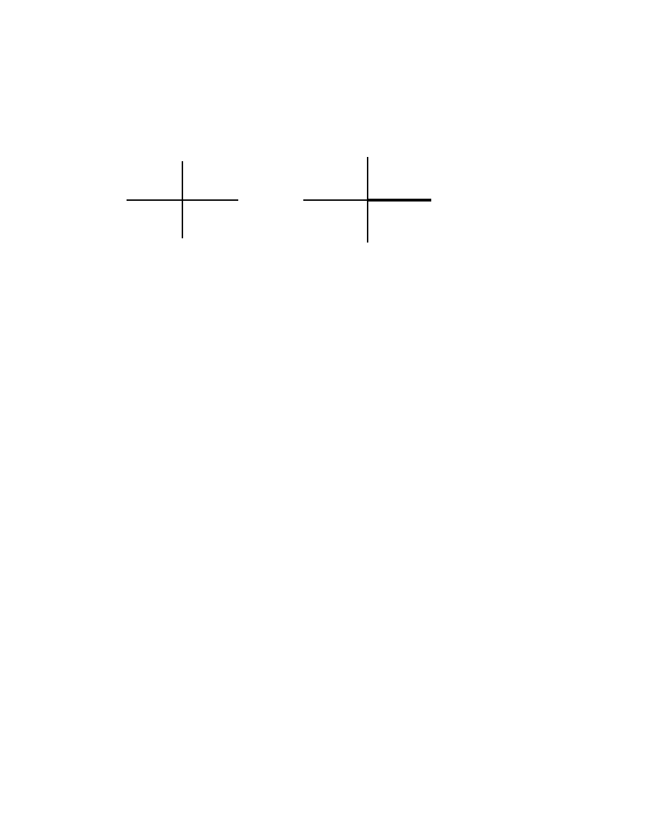
Fig. 4. Stereographic, or radial, compactification of
R
n
.
1.8 Radial compactification
One point of view that I would like to emphasize from the beginning of
these lectures is that non-compact spaces, such as R
n
, should generally
be compactified. The idea here is simply that I do not want to think
of asymptotic expansions such as (1.13) as some new phenomenon tak-
ing place ‘at infinity.’ Rather this is just a form of Taylor’s theorem at
the boundary (which is ‘infinity’). To see this just carry out the stereo-
graphic, or perhaps more correctly radial, compactification of Euclidean
space, R
n
, to a ball, or better yet a half-sphere as in Figure 4
S
n
+
= {z
′
∈ R
n+1
; |z
′
| ≤ 1, z
′
1
≥ 0}.
(1.47)
Stereographic projection is the identification of R
n
with the interior of
the half-sphere:
SP : R
n
∋ z 7−→ z
′
=
1
(1 + |z|
2
)
1
2
,
z
(1 + |z|
2
)
1
2
∈ S
n
+
⊂ R
n+1
.
(1.48)
I shall consistently denote by x a defining function
41
for the boundary of
a manifold with boundary. In this case x = z
′
1
= (1+|z|
2
)
−
1
2
is a defining
function for the boundary of S
n
+
. In |z| > 1, (1+|z|
2
)
1
2
= |z|
−1
(1+|z|
−2
)
1
2
41
A defining function for a hypersurface H in a manifold M is a real-valued function
ρ ∈ C
∞
(M ) which vanishes precisely on H, so H = {p ∈ M ; ρ(p) = 0} and has
dρ(p) 6= 0 at all points of H. For the boundary of a manifold with boundary I shall
assume that x is normalized to be positive in the interior of M.

16
Euclidean Laplacian
and it follows that |z|
−1
is a boundary defining function for S
n
+
, except for
the minor problem that it blows up at the interior point corresponding to
the origin in R
n
. This means that (1.13) can be rewritten in the form
42
Φ
0
(λ)g = SP
∗
f where
f = e
iλ/x
x
1
2
(n−1)
h
+
+ e
−iλ/x
x
1
2
(n−1)
h
−
with h
±
∈ C
∞
(S
n
+
).
(1.49)
The asymptotic expansion (1.13) follows from the Taylor expansion of
the functions h
±
43
at the boundary of S
n
+
.
44
The Sommerfeld radiation
condition can be written
(x
2
∂
∂x
− iλ)u ∈ L
2
sc
(S
n
+
)
(1.50)
where L
2
sc
(S
n
+
) is the space of square-integrable functions for the metric
volume form, L
2
(R
n
) = SP
∗
L
2
sc
(S
n
+
).
I will note here, for later reference, the form of the Euclidean metric
as a metric on the interior of S
n
+
. Introducing polar coordinates on R
n
,
θ = z/|z|, R = |z| the metric becomes
|dz|
2
= dR
2
+ R
2
|dθ|
2
(1.51)
where |dθ|
2
denotes the usual metric on the sphere S
n−1
. If x = |z|
−1
is
the boundary defining function discussed above then the metric can be
written, near the boundary, in the form
|dz|
2
=
dx
2
x
4
+
|dθ|
2
x
2
.
(1.52)
Generalizations of this type of metric, and the associated scattering
theory, to an arbitrary compact manifold with boundary in place of
S
n
+
will be discussed in Lecture 6.
42
For f a function on S
n
+
, the pull-back to R
n
is SP
∗
f = f ◦ SP .
43
Notice that C
∞
(S
n
+
) is the space of functions on S
n
+
which are continuous up to
the boundary with all their derivatives. Thus demanding h ∈ C
∞
(S
n
+
) is the same
as saying that h =
e
h
¯
S
n
+
for some function
e
h ∈ C
∞
(S
n
).
44
Conversely (1.49) can be deduced from (1.13), together with similar estimates on
formal derivatives of the expansion.

2
Potential scattering on R
n
The simplest perturbations of the flat Laplacian on Euclidean space are
given by potentials. I will spend this second lecture showing the degree
to which the results I described last time, for the flat case, extend when
the Laplacian is perturbed in this way. One reason I wish to concentrate
on potential perturbations is their simplicity, which means that I can
even outline the methods of proof. Much of what I will say carries over
to other perturbations and I shall say a little more about this later.
So consider the operator ∆ + V where V ∈ C
∞
c
(R
n
). Here V acts
by multiplication and is the ‘potential.’
1
I shall limit myself to this
simple case, where V is both smooth and has compact support, even
though most of the results I describe have generalizations involving less
regularity or less stringent support properties (e.g. replaced by growth
conditions at infinity). In fact much energy has gone into refining these
results for low regularity potentials with weak decay conditions at infin-
ity.
2.1 The resolvent of
∆ + V
The true spectral theory of ∆ + V is very simple. Namely the new
operator is almost unitarily equivalent to the free one. As in the free
case, rather than discuss the technicalities of the fact that ∆ + V is an
unbounded self-adjoint
2
operator on L
2
(R
n
), I shall simply discuss the
resolvent family.
1
For the most part I shall assume that V is real-valued even though this is not
always necessary.
2
For real V. The notes of Simon’s lectures [17] contain a good treatment of con-
ditions on a potential (much more general than smooth with compact support)
guaranteeing that ∆ + V is self-adjoint.
17

18
Potential scattering on R
n
Proposition 2.1
For each λ ∈ C , Im λ << 0,
3
there is a uniquely
defined operator R
V
(λ) : S(R
n
) −→ S(R
n
) such that
(∆ + V − λ
2
) ◦ R
V
(λ) = Id .
(2.1)
Indeed from the construction, via analytic Fredholm theory, that I
will outline much more can be said about the family R
V
(λ). The ra-
dial compactification of R
n
to a ball, or half-sphere, reduces S(R
n
) to
˙
C
∞
(S
n
+
), the space of smooth functions on S
n
+
vanishing with all deriva-
tives at the boundary, i.e. S(R
n
) = SP
∗
˙
C
∞
(S
n
+
). Thus, for Im λ < 0,
R
V
(λ) : ˙
C
∞
(S
n
+
) −→ ˙C
∞
(S
n
+
).
4
Proposition 2.2
For f ∈ C
∞
c
(R
n
) ⊂ ˙C
∞
(S
n
+
), n ≥ 2,
R
V
(λ)f = R
0
(λ)G
V
(λ)f with G
V
(λ) extending to be
meromorphic in λ as a map G
V
(λ) : C
∞
c
(R
n
) −→ C
∞
c
(R
n
).
(2.2)
Here λ ∈ C if n is odd and λ ∈ Λ if n is even.
In fact even more can be said, namely that G
V
(λ) has finite rank residues
at each pole and that these residues are smoothing operators, having
kernels in C
∞
(R
n
× R
n
).
Proof
The construction of R
V
(λ) proceeds via perturbation theory
(which is why it is so easy) and then the extra properties follow from
analytic Fredholm theory. Observe that, for n > 1, the corresponding
operator R
0
(λ) has these properties and no poles at all.
Starting from the desired identity (2.1), and the corresponding free
identity, it follows that
R
0
(λ) = R
0
(λ) ◦ (∆ + V − λ
2
) ◦ R
V
(λ) = R
V
(λ) + R
0
(λ) ◦ V ◦ R
V
(λ).
(2.3)
This can be written (Id +R
0
(λ) ◦ V )◦R
V
(λ) = R
0
(λ). Without worrying
for the moment about whether it makes sense, it is only necessary to
invert the operator Id +R
0
(λ) ◦ V and then
5
R
V
(λ) = (Id +R
0
(λ) ◦ V )
−1
R
0
(λ).
(2.4)
3
That is, Im λ < c(V ) for some constant c(V ) depending on V. There can be only
a finite number of poles of R
V
(λ) in Im λ < 0. If V is real they must lie on the
negative imaginary axis.
4
I will generally identify an operator on S(R
n
) with the operator on ˙
C
∞
(S
n
+
) to
which it is conjugated by SP
∗
.
5
This is often called the Lipmann-Schwinger equation, as are several other closely
related equations.

2.1 The resolvent of ∆ + V
19
Now, I need to do a little functional analysis to see this. First consider
the Hilbert space e
T |z|
L
2
(R
n
), meaning the space of functions of the
form e
T |z|
f(z) where f is square-integrable. Let L
2
c
(B(R)) be the space
of square-integrable functions on R
n
with support in the ball of radius
B(R) = {|z| ≤ R}. In the region of C or Λ, depending on the parity
of the dimension, where | Imλ| < T, R
0
(λ) defines a family of compact
operators
6
R
0
(λ) : L
2
c
(B(R)) −→ e
T |z|
L
2
(R
n
)
(2.5)
depending holomorphically on λ. Furthermore the norm of this operator
tends to zero as λ → −i∞ in the original ‘physical’ half-plane, P. Since
V has compact support, if R is taken to be large enough then V :
e
T |z|
L
2
(R
n
) −→ L
2
c
(B(R)). Now ‘analytic Fredholm theory’
7
shows that
the inverse family
(Id +R
0
(λ) ◦ V )
−1
: e
T |z|
L
2
(R
n
) −→ e
T |z|
L
2
(R
n
)
(2.6)
is meromorphic with all residues of its inverse being operators of finite
rank. In particular this inverse exists for all λ outside a discrete set. The
uniqueness of the inverse in the physical region shows that enlarging T
gives an extension of the same family. Finally this shows the existence
of R
V
(λ), given by (2.4).
8
I still need to check the stated properties of R
V
(λ), in particular (2.2).
Instead of (2.3) the similar identity, arising from the fact that R
V
(λ) is
expected to be a two-sided inverse, can be used:
R
0
(λ) = R
V
(λ) ◦ (∆ + V − λ
2
) ◦ R
0
(λ) = R
V
(λ) + R
V
(λ) ◦ V ◦ R
0
(λ).
(2.7)
Now the operator
Id +V ◦ R
0
(λ) : L
2
c
(B(R)) −→ L
2
c
(B(R))
(2.8)
6
The exponential bound follows from the estimates on R
0
(λ) discussed in Lecture 1.
The compactness is a form of the Ascoli-Arzela theorem, for the embedding of
Sobolev spaces.
7
The fact that a compact operator, such as R
0
◦ V, is norm-approximable by finite
rank operators shows the invertibility of Id +R
0
(λ) ◦ V is, locally in λ, equivalent
to the invertibility of a matrix and hence to the invertibility of a function (the
determinant of the matrix.) Thus if the family is invertible at one point, as it is
in this case, it is invertible outside a discrete set at which the inverse family has
poles.
8
The composition here makes sense since (Id +R
0
(λ) ◦ V )
−1
: e
T |z|
L
2
(R
n
) −→
e
T |z|
L
2
(R
n
) for any T large enough compared with |λ|.

20
Potential scattering on R
n
is entire with a meromorphic inverse which is just G
V
(λ). It is also the
case that if f ∈ ˙C
∞
(B(R)) then
9
G
V
(λ)f = (Id +V ◦ R
0
(λ))
−1
f ∈ ˙C
∞
(B(R))
(2.9)
depends meromorphically on λ. This leads to (2.2). That this construc-
tion gives the same operator R
V
(λ) follows from the invertibility near
−i∞.
2.2 Poles of the resolvent
The poles of the analytic continuation of the resolvent are in many ways
similar to the eigenvalues of the Laplacian on a compact manifold with
boundary, except that they are not real! They will be discussed at
greater length in Lecture 4 but for the moment I simply note that they
are associated to generalized eigenfunctions. Indeed it follows from (2.2)
that, for n odd, if the resolvent R
V
has a pole at λ then there is an
eigenfunction u of the form
u = exp(−iλ/x)x
1
2
(n−1)
w, w ∈ C
∞
(S
n
+
), (∆ + V − λ
2
)u = 0.
(2.10)
In the even-dimensional case the same is true in the physical region, but
the generalized eigenfunctions corresponding to poles of the resolvent
are not quite so simple. However they can be characterized in a uniform
way:
Lemma 2.1
10
For n ≥ 2, λ is a pole of R
V
(λ) if and only if there
is a non-trivial solution, u ∈ C
∞
(R
n
), to (∆ + V − λ
2
)u = 0 such that
u = −R
0
(λ)V u.
If Im λ < 0 then a function of the form (2.10) is square-integrable.
If Im λ > 0 it is not, nor is it for 0 6= λ ∈ R, unless the coefficient, w,
9
This is ‘elliptic regularity.’ The operator R
0
(λ) maps H
p
c
(R
n
) into H
p+2
loc
(R
n
) for
any λ and p, where H
p
c
(R
n
) and H
p
loc
(R
n
) are, respectively, the spaces of functions
with compact support in, and locally in, the Sobolev space H
p
(R
n
).
10
This characterization follows directly from (2.2). Namely, if R
V
(λ) has a pole,
then so must G
V
(λ)f for some f ∈ C
∞
c
(R
n
). Since (Id +V ◦ R
0
(λ))G
V
(λ) = Id
the residue, u
′
∈ C
∞
c
(R
n
), of G
V
(λ)f must satisfy u
′
+ V R
0
(λ)u
′
= 0. Then
u = R
0
(λ)u
′
satisfies u = −R
0
(λ)V R
0
(λ)u
′
= −R
0
(λ)V u. Conversely if there is
such a function u ∈ C
∞
(R
n
), then g = V u ∈ C
∞
c
(R
n
) satisfies g = −V R
0
(λ)g
which means that Id +V ◦ R
0
(λ) has null space and therefore cannot be invertible,
so G
V
(λ), and hence R
V
(λ), must have a pole.

2.3 Boundary pairing
21
vanishes at the boundary. The real axis in λ is of particular interest
since this gives rise to the spectrum of ∆ + V.
I shall summarize the ‘algebraic’ information in the poles in the fol-
lowing terms.
Definition 2.1
Let D(V ) ⊂ C × N, for n odd, or D(V ) ⊂ Λ × N for n
even, be the divisor defined by R(λ). Thus (λ
′
, k) ∈ D(V ) if R(λ) has a
pole at λ = λ
′
of rank
11
k.
2.3 Boundary pairing
As a continuation to Lemma 2.1 let me note the ‘absence of embedded
eigenvalues:’
Proposition 2.3
For any n, and V ∈ C
∞
c
(R
n
) real-valued, there are no
non-trivial solutions to (2.10) with 0 6= λ ∈ R.
Note that, for either parity of n, when 0 6= λ ∈ R the residue of
any pole at λ must satisfy (2.10). There are two parts to the proof of
Proposition 2.3. The first part is to show that if u satisfies (2.10) then
it is actually in ˙
C
∞
(S
n
+
), i.e. S(R
n
). This argument in turn consists of
two steps. First it will be seen from a general ‘boundary pairing,’ which
arises as a form of Green’s formula, that w = 0 on S
n−1
= ∂S
n
+
. Then
an inductive argument will be used to show that the whole Taylor series
vanishes, so u ∈ ˙C
∞
(S
n
+
).
To define the boundary pairing, consider a more general ‘formal solu-
tion’ than in (2.10). Namely suppose that
u = u
+
+ u
−
, u
±
= exp(±iλ/x)x
1
2
(n−1)
w
±
, w
±
∈ C
∞
(S
n
+
) and
(∆ + V − λ
2
)u = f ∈ ˙C
∞
(S
n
+
).
(2.11)
11
This is the algebraic multiplicity of the pole. In this context it can be defined as
the dimension of the subspace of C
∞
(R
n
) which is the sum of the ranges of all
the singular terms in the Laurent series for R
V
(λ) at λ = λ
′
. For λ 6= 0 this is
the same as the range of the residue, i.e. the least singular term. All the elements
of this space are annihilated by (∆ − (λ
′
)
2
)
k
. See also the paper of Gohberg and
Sigal [28].
22
Potential scattering on R
n
.........
.
.
.
.
.
.
.
.
.
.
.
.
.
.
.
.
.
.
.
.
.
.
.
.
.
.
.
.
.
.
.
......
......
................
...
..
.
...
...
..
.
...
.
×
×
×
×
×
×
×
.......... ..........
.......... ..........
.......... ..........
.......... ..........
.......... .........
. ..........
..........
..........
..........
..........
..........
..........
..........
..........
.........
.
.
.
.
.
.
.
.
.
.
.
.
.
.
.
.
.
.
.
.
.
.
.
.
.
.
.
.
.
.
.
.
.
.
.
.
.
.
.
.
.
.
.
.
.
.
.
.
.
.
.
.
.
.
.
.
.
.
.
.
.
.
.
.
.
.
.
.
.
.
.
.
.
.
.
.
.
.
.
.
.
.
.
.
.
.
.
.
.
.
.
.
.
.
.
.
.
.
.
.
.
.
.
.
.
.
.
.
.
.
.
.
.
.
.
.
.
.
.
.
.
.
.
.
.
.
.
.
.
.
.
.
.
.
.
.
.
.
.
.
.
.
.
.
.
.
.
.
.
.
.
.
.
.
.
.
.
.
.
.
.
.
.
.
.
.
.
.
.
.
.
.
.
.
.
.
.
.
.
.
.
.
.
..
.
.
.
.
.
.
.
.
.
.
.
.
.
.
Re λ
Im λ
Fig. 5. Poles of the analytic continuation of R
V
(λ) (n odd)
Lemma 2.2
12
Suppose u
(i)
for i = 1, 2 are as in (2.11), V ∈ C
∞
c
(R
n
)
is real-valued and 0 6= λ ∈ R then
−2iλ
Z
S
n−1
v
(1)
+
v
(2)
+
− v
(1)
−
v
(2)
−
dz =
Z
R
n
f
(1)
u
(2)
− u
(1)
f
(2)
dz
where v
(i)
±
= w
(i)
±
¯
∂S
n
+
.
(2.14)
Applying (2.14) directly to u as in (2.10) it follows that the leading
coefficient v = v
+
= w
¯
∂S
n
+
vanishes identically.
12
To prove this, choose a ‘cut-off ’ function ρ ∈ C
∞
c
(R) which has ρ(x) = 1 for |x| < 1
and support in |x| ≤ 2. Now consider the integral
I
ǫ
=
Z
Rn
f
(1)
u
(2)
− u
(1)
f
(2)
ρ(ǫ|z|)dz.
(2.12)
Clearly, as ǫ ↓ 0 this converges to the right side of (2.14). Inserting f
(i)
= (∆ +
V − λ
2
)u
(i)
the terms involving V and λ
2
cancel. Integration by parts and use of
the given form (2.11) shows that I
ǫ
converges to the left side of (2.14). If V is not
real then an alternative version of (2.14) is still available:
−2iλ
Z
S n−1
v
(1)
+
v
(2)
−
− v
(1)
−
v
(2)
+
=
Z
Rn
f
(1)
u
(2)
− u
(1)
f
(2)
dz.
(2.13)

2.4 Formal solutions
23
2.4 Formal solutions
Consider the structure of a formal solution as in (2.11). Since V has
compact support this has nothing to do with V at all, i.e. u
±
are just
formal solutions of the free Laplacian in the sense that ∆u
±
= f
±
∈
S(R
n
).
Lemma 2.3
13
For each h ∈ C
∞
(S
n−1
) and 0 6= λ ∈ R there is an
element, u ∈ C
∞
(R
n
), of the formal null space of ∆−λ
2
, i.e. (∆−λ
2
)u ∈
S(R
n
), having an asymptotic expansion
u ∼ exp(iλ|z|)|z|
−
1
2
(n−1)
X
j≥0
|z|
−j
h
j
(θ), z = |z|θ with h
0
= h.
(2.15)
Moreover the difference of any two elements of the formal null space
satisfying (2.15) is in S(R
n
).
2.5 Unique continuation
The remainder of the argument needed to prove Proposition 2.3 is a
unique continuation theorem:
Theorem 2.1
14
If 0 6= λ ∈ R then any function u ∈ ˙C
∞
(S
n
+
) satisfying
(∆ + V − λ
2
)u = 0 vanishes identically.
13
To see the existence of u consider (L1.9) and (1.14). This certainly gives a formal
solution (indeed a solution) of the form (2.11) with leading coefficient in u
+
being
h. Using Borel’s lemma (see [40], Theorem 1.2.6) at the boundary of S
n
+
, the
coefficients |z|
−j
h
+
j
= x
j
h
+
j
can be summed, uniquely modulo S(R
n
) = ˙
C
∞
(S
n
+
),
to give a solution of the form (2.15). The uniqueness follows by noting that if
u has an expansion as in (2.15) with leading term, h, identically zero then u is
square-integrable. Taking the Fourier transform of the equation (∆ − λ
2
)u = f it
follows that (|ζ|
2
− λ
2
)
−1
b
f must be square-integrable and hence
b
f must vanish on
{|ζ|
2
= λ
2
}. This shows that u ∈ S(R
n
).
14
This result is valid for complex-valued V ∈ C
∞
c
(R
n
). To prove it consider an
eigenfunction u ∈ S(R
n
), which therefore satisfies (∆ − λ
2
)u = −V u = f ∈
C
∞
c
(R
n
). The first step is to show that this implies that u ∈ C
∞
c
(R
n
), i.e. u vanishes
near infinity. There are several ways to see this, one is to use the expansion of u
in spherical harmonics. Each of the coefficients in this expansion is a function of
r = |z| which is rapidly decreasing and satisfies an ordinary differential equation. It
can be seen that the equation is a form of Bessel’s equation which has no non-trivial
rapidly decreasing solution. Another proof can be based on the characterization
of the range of the Radon transform and is briefly discussed in Footnote 3.5.
Once such a putative eigenfunction corresponding to an embedded eigenvalue is
known to have compact support it can be shown to vanish identically using the
unique continuation of solutions to second order elliptic equations.

24
Potential scattering on R
n
This completes the proof of Proposition 2.3. Thus, if V is real-valued
15
then R
V
(λ) is well defined for all real, non-zero, λ.
2.6 Perturbed plane waves
I am now in a position to describe the construction of analogues of the
‘plane wave’ eigenfunctions Φ
0
(z, ω, λ) = exp(iλz · ω) in the free case.
Lemma 2.4
For each 0 6= λ ∈ R and ω ∈ S
n−1
there is a unique
function in the null space of ∆ + V − λ
2
of the form
Φ
V
(z, ω, λ) = exp(iλz · ω) + exp(−iλ|z|)|z|
−
1
2
(n−1)
φ
V
(z, ω, λ)
with φ
V
∈ C
∞
(S
n
+
).
(2.16)
Proof The compactness of the support of V means that (∆ + V −
λ
2
)e
iλz·ω
= f with f = −V e
iλz·ω
∈ C
∞
c
(R
n
). Since R
V
(λ) has no pole
on R\ {0},
Φ
V
(z, ω, λ) = exp(iλz · ω) + R
V
(λ)f
(2.17)
is, by (2.2) and Proposition 1.1, of the form (2.16) and satisfies (∆ +
V − λ
2
)Φ
V
= 0. The uniqueness follows from Proposition 2.3, since the
difference between two solution of the form (2.16) would be of the form
(2.10).
Notice that Φ
V
(z, ω, λ), defined by (2.17) extends to be meromorphic
as a function of λ on the same domain as R
V
(λ).
2.7 Relative scattering matrix
The coefficient in (2.16) also depends smoothly
16
on the parameters, i.e.
φ
V
(z, ω, λ) ∈ C
∞
(S
n
+
× S
n−1
× (R\ {0})).
Thus, as with (1.9) in the free case, Φ
V
can be used as the kernel of an
operator into the null space of ∆ + V − λ
2
:
15
If V is complex-valued then it is possible for there to be poles of the resolvent at
points in the continuous spectrum, but the corresponding eigenfunctions cannot
be square-integrable.
16
In fact φ
V
is a real-analytic function of ω and λ on this set, see Footnote 26.

2.7 Relative scattering matrix
25
Φ
V
(λ)g =
Z
S
n−1
Φ
V
(z, ω, λ)g(ω)dω.
(2.18)
From the form of Φ
V
in (2.17) and (1.13) it follows that Φ
V
(λ)g has,
for g ∈ C
∞
(S
n−1
), a similar asymptotic expansion
Φ
V
(λ)g(|z|θ) = e
iλ|z|
(λ|z|)
−
1
2
(n−1)
e
−
1
4
π(n−1)i
(2π)
1
2
(n−1)
g(θ)
+e
−iλ|z|
(λ|z|)
−
1
2
(n−1)
e
1
4
π(n−1)i
(2π)
1
2
(n−1)
g
′
(θ) + u
′
, u
′
∈ L
2
(R
n
).
(2.19)
In fact it has a complete asymptotic expansion of which I have written
only the leading part. Thus for the perturbed problem ∆ + V, with
V ∈ C
∞
c
(R
n
) real-valued, there is a complete analogue of Lemma 1.2, i.e.
a solution of (∆+V −λ
2
)u = 0 of the form (1.15) for each h ∈ C
∞
(S
n−1
).
Again from the uniqueness result, h
′
(θ) is determined by h. The map
A
V
(λ)h = h
′
maps C
∞
(S
n−1
) into itself. In fact, as follows from (2.19),
it is of the form
A
V
h(θ) = i
(n−1)
h(−θ) +
Z
S
n−1
A
′
V
(θ, ω, λ)h(ω)dω
(2.20)
where A
′
V
∈ C
∞
(S
n−1
× S
n−1
× (R\ {0})). The operator A
V
(λ) is the
absolute scattering matrix.
17
From (2.16), (2.18) and (2.19),, for λ > 0,
A
′
V
(θ, ω, λ) = e
1
4
π(n−1)i
(2π)
−
1
2
(n−1)
λ
1
2
(n−1)
φ
V
(θ, ω, λ).
(2.21)
As noted earlier it is usual to normalize away the scattering matrix
for Euclidean space, and to define the scattering matrix
18
by
S
V
(θ, ω, λ)g =
i
−(n−1)
A
V
(λ)g
(−θ).
(2.22)
Thus it follows that the scattering matrix is of the form Id +B
V
where
B
V
is a smoothing operator, i.e. has C
∞
Schwartz’ kernel. This kernel
is called the scattering amplitude. Needless to say it carries the same
information as A
V
or S
V
.
17
I know, it is not a matrix, but this is by extrapolation from the 1-dimensional case
where it is. Blame the physicists. The obvious alternative name, the ‘scattering
operator,’ is reserved for the t-convolution operator with kernel obtained by Fourier
transformation of the λ variable.
18
I shall call this the relative scattering matrix.

26
Potential scattering on R
n
2.8 Asymptotics of the resolvent
The generalized plane waves also give the leading term in the asymptotic
expansion of R
V
(λ)f, just as in Proposition 1.1 in the free case.
Proposition 2.4
For f ∈ ˙C
∞
(S
n
+
) and λ > 0
R
V
(λ)f = e
−iλ|z|
|z|
−
1
2
(n−1)
w(z),
with w = (SP
∗
)(w
′
), w
′
∈ C
∞
(S
n
+
) and
v = w
′
¯
S
n−1
=
1
2iλ
P
†
V
(λ)f =
1
2iλ
Z
R
n
P
†
V
(z
′
,
z
|z|
, λ)f(z
′
)dz
′
where P
V
(z
′
; ω, λ) = λ
1
2
(n−1)
e
1
4
π(n−1)i
(2π)
−
1
2
(n−1)
Φ
V
(z, ω, λ).
(2.23)
Proof To check (2.23) first notice that the boundary pairing, (2.13),
whilst proved for two solutions as in (2.11), is also valid, with the same
proof, when u = u
(1)
= R
V
(λ)f is as in (2.11) but u
(2)
= Φ
V
(λ).
19
This
gives the identity
2iλλ
−
1
2
(n−1)
e
−
π
4
(n−1)i
(2π)
1
2
(n−1)
v =
Z
f(z)Φ
V
(z, ω, λ)dz.
(2.24)
Here v is the boundary value of w
′
= R
V
(λ)f in (2.2). This gives (2.23).
As in the free case, P
V
(λ) is the Poisson operator, so that if g ∈
C
∞
(S
n−1
) then u = P
V
(λ)g is the unique solution of (∆ + V − λ
2
)u = 0
with an expansion as in (2.11) with v
+
¯
S
n−1
= g. Also, the difference of
the resolvent at ±λ on the real axis can be recovered from the perturbed
plane waves:
20
R
V
(λ) − R
V
(−λ) = λ
n−2
M
V
(λ) =
1
2i
(2π)
−(n−1)
λ
n−2
Φ
V
(λ)Φ
†
V
(−λ).
(2.26)
19
Just integrate against a smooth function in the ω variable.
20
Let u be the solution to (∆ + V − λ
2
)u = 0 obtained by applying R
V
(λ) − R
V
(−λ)
to f ∈ C
∞
c
(R
n
). Thus u has an expansion as in (2.11) and v
+
, the boundary value
of w
+
, which is just the boundary value of −R
V
(−λ)f, is given by
1
2iλ
λ
1
2
(n−1)
e
−
1
4
π(n−1)i
(2π)
−
1
2
(n−1)
Φ
†
V
(−λ)f.
(2.25)
The solution with this boundary value is obtained by applying P
V
(λ) and this is
just the right side applied to f. It follows that the two sides of (2.26) are equal as
operators.

2.9 L
2
eigenfunctions
27
2.9
L
2
eigenfunctions
The poles of the resolvent in the physical half-plane are the easiest to an-
alyze. Indeed, since R
V
(λ) is holomorphic and acts on S(R
n
) in a deleted
neighbourhood of such a point it follows that the residue operators
21
also
acts on S(R
n
). Its range is the corresponding eigenspae. Provide V is
real, any poles in the physical half-plane are necessary simple and lie on
the imaginary axis.
22
Conversely any L
2
eigenfunction of ∆ + V corre-
sponding to a negative eigenvalue, σ, gives rise to a pole of the resolvent
R
V
(λ) at the unique point λ ∈ P with λ
2
= σ.
2.10 Zero energy states
All the L
2
eigenfunctions of ∆ + V are known as ‘bound states’ in the
physical literature. As well as those arising from negative eigenvalues
there may be ‘zero energy’ states, i.e. elements of the null space of
∆ + V. For n odd, R
V
(λ)
23
can have at most a double pole at 0.
24
The
leading coefficient, i.e. the coefficient of λ
−2
, maps onto the null space
of ∆ + V acting on L
2
(R
n
).
25
The residue space, being the linear span
of the coefficients of λ
−1
in the expansion of R
V
(λ)f, for f ∈ C
∞
c
(R
n
)
such that there is no λ
−2
term, consists of elements of the null space
of ∆ + V which are not in L
2
(R
n
). For n = 3 this space is at most one
21
Meaning the coefficients in the Laurent expansion of the operator near a pole
e
λ :
R
V
(λ) =
X
j≤p
(λ −
e
λ)
−j
B
j
+ B
′
(λ),
B
′
(λ) holomorphic near
e
λ.
(2.27)
22
That is, of order 1, i.e. j = 1 in (2.27). This follows from the self-adjointness,
which is to say that for any φ ∈ S(R
n
)
|
Z
Rn
φ(∆ + V − λ
2
)φdz| ≥ 2| Im λ|| Re λ|kφk
2
L
2
=⇒ kφk
L
2
≤ (2| Im λ|| Re λ|)
−1
k(∆ + V − λ
2
)φk
L
2
(2.28)
23
For V real-valued.
24
This follows from the inequality (2.28).
25
That it takes values in the L
2
null space of ∆ + V follows from (2.28). To see
that it is surjective observe that if u ∈ L
2
(R
n
) satisfies (∆ + V )u = 0 then
∆u = −V u ∈ C
∞
c
(R
n
). This implies that u = −R
0
(0)V u and that V u cannot
vanish identically so (Id −V R
0
(λ))
−1
V u must have a double pole at 0, the leading
coefficient of which is V u. This shows that u occurs as the leading coefficient in
R
V
(λ)u.

28
Potential scattering on R
n
dimensional and its non-zero elements are called ‘half-bound states;’
they do not occur if n ≥ 5.
2.11 Meromorphy of the scattering matrix
The meromorphic continuation of the resolvent, to C for odd dimensions
and to Λ for even dimensions, has been discussed above. From this it
can be deduced that the scattering matrix has a similar continuation:
Proposition 2.5
26
The relative scattering matrix for V ∈ C
∞
c
(R
n
) ex-
tends to a meromorphic function of λ ∈ C for n odd and to a meromor-
phic function of λ ∈ Λ for n even; the poles of the analytic continuation
are among the poles of R
V
(λ) with at most the same multiplicity.
26
The Lipmann-Schwinger equation can be used to express the scattering matrix in
terms of the resolvent. Thus, the kernel of the scattering matrix is, for λ > 0, the
product of λ
1
2
(n−1)
e
1
4
π(n−1)i
(2π)
−
1
2
(n−1)
and the coefficient of e
−iλ|z|
|z|
−
1
2
(n−1)
in the expansion of Φ
V
(λ) as |z| → ∞. Writing Φ
V
as
Φ
V
(λ) = Φ
0
(λ) − R
0
(λ)V Φ
0
(λ) + R
0
(λ)V R
V
(λ)V Φ
0
(λ)
(2.29)
it follows that
A
V
(λ) = A
0
(λ) −
1
2iλ
P
†
0
(V Φ
0
(λ) − V R
V
(λ)V Φ
0
(λ)) , for λ > 0.
(2.30)
The compactness of the support of V means that the right side extends to a
meromophic function of λ, in C or Λ depending on the parity of the dimension. It
follows that the poles of A
V
(λ) must occur at poles of R
V
(λ) and with no greater
multiplicity.

3
Inverse scattering
In this lecture I shall discuss three main types of inverse scattering re-
sults. I shall ignore the case n = 1
1
since this has an enormous literature,
the methods available then are somewhat different
2
and the results are
more precise and complete. The three basic results examined here cor-
respond to different parts of the scattering matrix. The first result,
showing in particular that the scattering matrix B
V
(θ, ω, λ) determines
V, arises from an examination of the high-frequency asymptotics, i.e. the
behaviour as λ → ∞, of B
V
. The second result shows that, for n ≥ 3,
the scattering amplitude B
V
(θ, ω, λ) for fixed 0 6= λ ∈ R also determines
V. Finally, in odd dimensions, the backscattering B
V
(−ω; ω, λ) defines
a globally Fredholm map, so at least near most points small variations
in the potential are determined by the scattering amplitude.
Before discussing these inverse results I shall briefly describe the Radon
transform and then its modification to the ‘Lax-Phillips transform,’
which is the name I am giving to the explicit form of their ‘translation-
representation’
3
for the free problem.
3.1 Radon transform
Since it is has other applications below and is in any case the basis for
the Lax-Phillips transform I shall first discuss the Radon transform. A
1
This is a beautiful theory. A good starting point to investigate it is the work of
Gel’fand and Levitan, [25].
2
The basic difference is related to the possibility of complexification to a problem
with one complex variable.
3
I have rather underemphasized the Lax-Phillips approach to scattering theory,
compared to its importance. This is partly because it cannot be applied without
serious modification to many problems that still fit within the scope of scattering
theory. Still it is an excellent paradigm. A brief discussion is given in Section 4.4.
29

30
Inverse scattering
hyperplane in R
n
is determined by its unit normal vector, ω, and signed
distance from the origin, s, where the sign is chosen so that sω is a point
in the hyperplane, a general point of which satisfies the linear equation
z · ω = s. This parametrization is 2-1, since (−s, −ω) parametrizes the
same hyperplane as (s, ω).
The Radon transform of u ∈ C
∞
c
(R
n
) is the integral over hyperplanes:
4
Ru(s, ω) =
Z
H={z·ω=s}
u(z)dH
z
∈ C
∞
c
(R× S
n−1
)
(3.1)
where dH
z
is the Euclidean measure induced on H. Notice that Ru(s, ω) =
0 in |s| > R if supp(u) ⊂ B(R). Clearly Ru(−s, −ω) = Ru(s, ω) so the
map u 7→ Ru is not surjective.
5
That it is injective can be seen by
relating it to the Fourier transform
6
:
bu(rω) =
∞
Z
−∞
e
−irs
Ru(s, ω)ds,
(3.6)
which is just the 1-dimensional Fourier transform in the s variable.
The Fourier inversion formula leads to the inversion formula for the
4
There is an extensive theory of generalized Radon transforms in several different
contexts. See Guillemin and Sternberg [30].
5
In fact the Radon transform is not surjective as a map from C
∞
c
(R
n
) to the even
subspace of C
∞
c
(R× S
n−1
). The precise range is given by a result of Helgason [36]:
Theorem 3.1
The range of the Radon transform as a map
R : ˙
C
∞
(B(R)) −→ ˙
C
∞
([−R, R] × S
n−1
),
(3.2)
for any
R > 0, consists of the functions satisfying
g(−s, −ω) = g(s, ω) ∀ s ∈ [−R, R], ω ∈ S
n−1
and
(3.3)
Z
s
k
g(s, ω)ds = P
k
(ω) is a polynomial of degree at most k, ∀ k.
(3.4)
6
Just introduce polar coordinates ξ = rω in the definition of the Fourier transform
to see that
b
u(rω) =
Z
e
−irω·z
f (z)dz
(3.5)
from which (3.6) follows, since dz = dHds when ω is fixed.

3.1 Radon transform
31
Radon transform
7
u(z) =
1
2
(2π)
−n+1
Z
S
n−1
(|D
s
|
n−1
Ru)(z · ω, ω)dω.
(3.10)
This also gives Plancherel’s formula
Z
R
n
|u(z)|
2
dz
=(2π)
−n+1
Z
R
Z
S
n−1
||D
s
|
1
2
(n−1)
Ru(s, ω)|
2
dωds, u ∈ C
∞
c
(R
n
).
(3.11)
Notice that the Radon transform extends by continuity to a map from
Schwartz space
8
R : S(R
n
) −→ S(R× S
n−1
).
(3.12)
There is a ‘uniqueness’ result for the Radon transform in this form which
is convenient to invoke below, also due to Helgason.
Proposition 3.1
9
If u ∈ S(R
n
) has Radon transform with support in
[−R, R] × S
n−1
then u ∈ ˙C
∞
(B(R)).
7
The Fourier inversion formula written in polar coordinates is
u(z) = (2π)
−n
Z
S n−1
∞
Z
0
e
iz·rω
b
u(rω)r
n−1
drdω.
(3.7)
Inserting (3.6) and using the fact that Ru is an even function to extend the integral
over r to negative values gives
u(z) =
1
2
(2π)
−n+1
Z
S n−1
1
2π
∞
Z
0
e
i(z·ω)r
∞
Z
−∞
Ru(s, ω)|r|
n−1
ds drd ω.
(3.8)
The 1-dimensional Fourier inversion formula then gives (3.10), with the operator
on functions in s being |D
s
|
n−1
= D
n−1
s
if n is odd or
|D
s
|
n−1
v(s) =
1
2π
∞
Z
−∞
e
irs
b
v(r)|r|
n−1
dr
(3.9)
if n is even.
8
The range space here consists of functions which are rapidly decreasing at infinity
and remain so after any differential operator with constant coefficients in the first
variable is applied.
9
The characterization of the range on S(R
n
) follows as in Footnote 5 with condition
(3.3) dropped, i.e. (3.4) holds for Ru whenever u ∈ S(R
n
). The injectivity of the
Radon transform then shows that Proposition 3.1 follows from Theorem 3.1.

32
Inverse scattering
3.2 Wave group
The solution properties of the wave equation are fundamental to the
study of the high-frequency behaviour of the scattering amplitude, and
for other reasons besides.
10
This is encoded in the existence, and prop-
erties, of the wave group for the operator ∆ + V :
11
Theorem 3.2
12
For any V ∈ C
∞
c
(R
n
) and any (u
0
, u
1
) ∈ C
∞
(R
n
) there
is a unique solution, u ∈ C
∞
(R× R
n
) to the Cauchy problem
(D
2
t
− ∆ − V )u(t, z) = 0 in R
t
× R
n
u(0, z) = u
0
(z), D
t
u(0, z) = u
1
(z) ∀ z ∈ R
n
(3.14)
and the resulting 2 × 2 matrix of operators
U
V
(t)
u
0
u
1
=
u(t, ·)
D
t
u(t, ·)
(3.15)
10
In the more ‘physical’ literature Schr¨
odinger’s equation
(D
t
+ ∆ + V )v = 0
(3.13)
is often used for similar purposes. The solution for the initial value problem
v(0) = v
0
is
v(t) = G(t)v
0
= exp(−i(∆ + V ))v
0
.
This defines a group of operators with infinitesimal generator −i(∆ + V ), which
explains the otherwise enigmatic statement in Footnote 1.2.
11
The discussion here is equally valid for the Laplacian of a Riemann metric on
a compact manifold, (provided |z − z
′
| is replaced by the Riemannian distance
between the points in (3.16)) with which the scattering case is compared at various
points below. The wave group for the Laplacian associated to a metric g will be
denoted U
g
(t).
12
There are a variety of different approaches to the proof of this important result.
For the case, actually under discussion here, of a potential perturbation of the flat
metric the proof, as usual, can be accomplished by perturbation from the flat case
where the solution can be written down using the Fourier transform, or explicitly.
Another approach, developed systematically by John [47] and followed in [81], is
to use the Radon transform to write the solution as a superposition of perturbed
plane waves. This is particularly suited to the requirements of Section 3.5 below.
Another method due to Hadamard [33] (see [44] Chapter 17 or for a more complete
account the book of Friedlander [22]), allows the solution to be written down quite
explicitly. The theory of Fourier integral operators gives a representation of the
solution somewhat intermediate between these two formulations; it is often the
most convenient. The existence, uniqueness and support properties of the solution
can also be obtained by less explicit functional-analytic methods, based on energy
estimates.

3.2 Wave group
33
forms a 1-parameter group
13
with infinitesimal generator
0
Id
∆ + V
0
;
the solution to (3.14) also satisfies the support estimate
14
supp(u) ⊂ {(t, z); ∃ z
′
∈ supp(u
0
) ∪ supp(u
1
) with |t| ≤ |z − z
′
|} .
(3.16)
One of the most important properties of the solution of the wave
equation is the manner in which singularities of the solution of the initial
value problem propagate. First note that the wave group extends by
continuity
15
to a group of operators
16
U
V
(t) : C
−∞
(R
n
) × C
−∞
(R
n
) −→ C
−∞
(R
n
) × C
−∞
(R
n
)
(3.17)
with the same support property, (3.16). In fact the solution to (3.14)
is an element of C
∞
(R
t
; C
−∞
(R
n
)).
17
In a weak form this can then be
stated as a bound on the singular support of the solution:
18
sing supp(u) ⊂
(t, z) ∈ R× R
n
; ∃
z
′
∈ sing supp(u
0
) ∪ sing supp(u
1
) with |z − z
′
| = |t|
.
(3.18)
In fact there is a much better way to describe such results, namely
in terms of the wavefront set.
19
For a distribution on R
k
this can be
considered as a subset
20
WF(u) ⊂ R
k
× S
k−1
.
(3.19)
The wavefront set WF(u) consists of those points (z, ω) such that the
Fourier transform of u localized near z is not rapidly decreasing in any
13
That these operators form a group, U
V
(t) · U
V
(t
′
) = U
V
(t + t
′
) follows from the
uniqueness of the solution to (3.14) and the t-translation invariance of the problem.
14
This is the ‘finite speed of propagation’ for solutions to the wave equation.
15
In the topology of distributions.
16
I denote by C
−∞
(R
n
) the usual space of distributions of unrestricted growth, i.e.
the dual space of C
∞
c
(R
n
) denoted by Schwartz D
′
(R
n
).
17
That is, it is a distribution in the spatial, z, variables which depends smoothly on
the time variable t.
18
That is, singularities travel only at the speed of ‘light.’ The singular support of a
distribution is the complement of the largest (there is a largest) open set to which
it restricts as a C
∞
function.
19
Introduced in this C
∞
setting by H¨
ormander [40].
20
The space here is to be thought of as the boundary of R
k
× S
k
+
where the second
factor is really the stereographic compactification of the dual R
k
. Thus, and this is
the more usual convention, WF(u) can be considered as a subset of R
k
× (R
k
\ {0})
which is ‘conic,’ i.e. invariant under the R
+
action on the second factor.

34
Inverse scattering
open cone containing the direction ω.
21
This notion allows (3.18) to be
elegantly improved to the two statements
22
WF(u) ⊂ {((t, z), (τ, ζ)) ∈ R
n+1
× S
n
; τ
2
= |ζ|
2
} and
(3.21)
((t, z), (τ, ζ)) ∈ WF(u) =⇒ (z + t
ζ
τ
,
ζ
|ζ|
) ∈ WF(u
0
) ∪ WF(u
1
).
(3.22)
The lines
t 7−→ (t, z − t
ζ
τ
, τ, ζ),
(3.23)
where τ
2
= |ζ|
2
as in (3.21), are the (null) bicharacteristics of the wave
operator.
23
Then (3.22) results from the two statements that WF(u) is a
complete union of such bicharacteristic curves and that a bicharacteristic
can only be in WF(u) if the point on it over t = 0 arises from a point in
WF(u
0
) ∪ WF(u
1
).
There is an intermediate space between the smooth functions of com-
pact support and the distributions on which the wave group is bounded.
Namely the finite energy space, H
FE
(R
n
), defined as the closure of
C
∞
c
(R
n
) × C
∞
c
(R
n
) with respect to the norm
k(u
0
, u
1
)k
2
=
Z
R
n
|ζ|
2
|b
u
0
(ζ)|
2
+ |b
u
1
(ζ)|
2
dζ
(3.24)
This is a Hilbert space,
H
FE
(R
n
) ⊂ S
′
(R
n
) × S
′
(R
n
),
(3.25)
on which U
V
(t) is a bounded group of operators.
21
More precisely, the complement R
k
× S
k−1
\ WF(u), of the wavefront set of u ∈
C
−∞
(R
k
) is defined as consisting of those points (z, ω) such that for some function
φ ∈ C
∞
c
(R
n
), with φ(z) 6= 0, and some function φ
′
∈ C
∞
(S
k−1
) with φ
′
(ω) 6= 0
the product of φ
′
and the Fourier transform, φ
′
(ω
′
)(
b
φu)(rω
′
) is uniformly rapidly
decreasing as r → ∞. This is an open condition, and hence WF(u) is a closed set;
its projection onto the first factor is the singular support
π
Rk
WF(u) = sing supp(u).
(3.20)
See for example [42].
22
This is almost a characterization of WF(u) for the solution to (3.14). If (z, ζ) ∈
WF(u
0
) ∪ WF(u
1
) then for at least one choice of sign, ((t, z ∓ tζ), (±
1
√
2
,
1
√
2
ζ)) ∈
WF(u).
23
That is, an integral curve of the Hamilton vector field 2τ ∂/∂t − 2ζ · ∂/∂z of the
symbol τ
2
− |ζ|
2
, of the wave operator.

3.3 Wave operators
35
3.3 Wave operators
There is an alternate definition of the scattering matrix, indeed an al-
ternative formulation of scattering theory itself, in terms of the wave
group.
24
Namely, for V ∈ C
∞
c
(R
n
) real valued, the limits
W
±
u = lim
t→±∞
U
V
(−t)U
0
(t)u, ∀ u = (u
0
, u
1
) ∈ (C
∞
c
(R
n
))
2
.
(3.26)
exist. This defines the Møller wave operators which extend by continuity
to isomorphisms from the finite energy space onto the orthocomplement
of the finite dimensional space spanned by the L
2
eigenfunctions, i.e.
onto the part of the finite energy space corresponding to the continuous
spectrum.
25
It is important that the two wave operators have the same
range since this means that the ‘abstract’ scattering operator can be
defined by:
e
S
V
= W
−1
+
◦ W
−
.
(3.27)
It is then a unitary operator, provided V is real, acting on the finite
energy space.
26
3.4 Lax-Phillips transform
The Radon transform satisfies the identity
27
R∆f = D
2
s
Rf
(3.29)
which effectively reduces the n-dimensional Laplacian to the one-dimen-
sional Laplacian. This is the basis of the Lax-Phillips transform which,
24
There is a similar formulation in terms of the group of operators solving the
Schr¨
odinger equation. That they give the same scattering operator (up to simple
renomalization) is part of Kato’s invariance principle [48]. For a development of
scattering theory on this basis see the book of Yafaev [117] and the lectures of
Simon [17].
25
This is called the ‘completeness’ of the wave operators.
26
The standard way of relating this scattering operator and the scattering matrix
defined earlier is to observe, from (3.26), that W
±
U
V
(t) = U
0
(t)W
±
, i.e. the
Møller wave operators intertwine the free and the perturbed wave group (acting
on the orthocomplement of the bound states). This means that
e
S
V
commutes
with U
0
(t) and so can be decomposed according to the spectral decomposition of
the free Laplacian. As one would expect
e
S
V
exp(iλz · ω) = exp(iλz · ω) +
Z
S n−1
B
V
(λ)(θ, ω) exp(iλz · θ)dθ.
(3.28)
27
To obtain this just apply the Laplacian to the inversion formula, (3.10), and then
apply the Radon transform.

36
Inverse scattering
for n odd, conjugates the free wave group U
0
(t) to a translation group.
Define
LP
u
0
u
1
= (2π)
−
1
2
(n−1)
D
1
2
(n+1)
s
(Ru
0
)(s, ω) − D
1
2
(n−1)
s
(Ru
1
)(s, ω)
.
(3.30)
The two terms, from u
0
and u
1
, have opposite parities under (s, ω) →
(−s, ω) so LP : C
∞
c
(R
n
)
2
−→ C
∞
c
(R× S
n−1
) is injective.
28
Proposition 3.2
For any odd n ≥ 3, the Lax-Phillips transform, (3.30),
conjugates the free wave group to the translation group:
LP ◦U
0
(t) ◦ LP
−1
= W
0
(t), W
0
(t)k(s, ω) = k(s − t, ω).
(3.31)
For any V ∈ ˙
C
∞
(B(R)) the transformed group
29
W
V
(t) = LP ◦U
V
(t) ◦ LP
−1
(3.32)
satisfies
W
V
(t)k(s, ω) = k(s − t, ω)
(
if s and s − t < −R
or s and s − t > R.
(3.33)
3.5 Travelling waves
The spectral, and scattering, properties of ∆ + V as λ → ∞ can be
expected to be classical, i.e. rather than involving global solutions of
differential equations the asymptotic behaviour should be expressible
in terms of local operations on V, and integration. To investigate the
high-frequency behaviour I shall use the wave equation and Lax-Phillips
transform.
The plane waves, e
iλz·ω
, on which much of the discussion up to this
point has been based, can be obtained by the one-dimensional (inverse)
Fourier transform:
e
iλz·ω
=
Z
R
e
−itλ
δ(t + z · ω)dt.
(3.34)
28
In fact it extends by continuity to an isometric isomorphism from the finite energy
space for the wave equation, defined in (3.25), onto L
2
(R× S
n−1
), this indeed is
the reason for the normalizing constant in (3.30).
29
In the odd-dimensional case the infinitesimal generator of the transformed group
W
V
(t) is D
s
+ V
LP
where V
LP
is the sum of a pseudodifferential operator of order
−1 and and an ‘anti-pseudodifferential’ operator of order −1, by which I mean
a pseudodifferential operator followed by the reflection (s, ω) → (−s, −ω). Both
terms can be taken to have kernels with support in the region |s|, |s
′
| ≤ R if V has
support in |z| ≤ R.

3.5 Travelling waves
37
Here δ(t + z · ω) ∈ S
′
(R
n+1
) is a distribution depending on ω ∈ S
n−1
as
a parameter:
hδ(t + z · ω), φi =
Z
R
n
φ(−z · ω, z)dz, φ ∈ S(R
n+1
).
(3.35)
By direct differentiation this distribution can be seen to be a solution of
the (free) wave equation:
(D
2
t
− ∆)δ(t + z · ω) = 0 in R
n+1
.
(3.36)
If now a potential is added then a natural generalization is to seek a
solution to the perturbed wave equation. Observe that the support of
the ‘travelling wave’ δ(t + z · ω) is disjoint from the support of V when
t << 0. Thus it makes sense to look for a perturbed travelling wave:
(D
2
t
− ∆ − V )u
V
(t, z, ω) = 0, u
V
(t, z, ω) = δ(t + z · ω) in t << 0.
(3.37)
This is the forcing problem for the wave equation.
Lemma 3.1
30
There is a unique solution to the forcing problem (3.37)
and, for some T > 0, exp(−T (1 + t
2
)
1
2
)u
V
∈ S
′
(R
n
).
31
The forced behaviour of the solution in t << 0, together with (3.16),
shows that for |z| ≤ R the solution u vanishes in t < −C − R for some
C depending on V. This, and the exponential bound, allows the Fourier-
Laplace transform to be taken.
Proposition 3.3
32
For Im λ << 0
Φ
V
(z, ω, λ) =
∞
Z
0
e
−itλ
u
V
(t, z, ω)dt
(3.38)
is the perturbed plane wave solution in Lemma 2.4.
33
30
The existence of the solution to this problem is equivalent to the solvability of the
Cauchy problem; as discussed in Section 3.2 above. For a more leisurely treatment
see [81].
31
The only reason that the solution is not tempered is that there may be L
2
eigenfunctions.
32
Certainly the Fourier-Laplace transform in (3.38) gives an element of the null space
of ∆ + V − λ
2
. That this solution is of the form (2.16) follows from the support
properties of u
V
.
33
The analytic continuation of Φ
V
(z, ω, λ) being given by (2.17).

38
Inverse scattering
A solution to (3.37), modulo C
∞
errors, can be found in the form of
a travelling wave with jump discontinuity:
34
u
′
V
(t, z, ω) = δ(t + z · ω) + H(t + z · ω)b(t, z, ω),
b ∈ C
∞
(R
n+1
× S
n−1
),
(3.40)
in the sense that (D
2
t
− ∆ − V )u
′
V
∈ C
∞
(R
n+1
× S
n−1
) and b = 0 in
t << 0. The Taylor series of b at t + z · ω = 0 is uniquely determined by
these conditions and
b(−z · ω, z, ω) = −
1
2
∞
Z
0
V (z + sω)ds.
(3.41)
The solution u
V
to the forcing problem is also of the form (3.40), with
b satisfying (3.41).
3.6 Near-forward scattering
From the construction of u
′
V
as a solution, modulo C
∞
, to the forc-
ing problem the high frequency asymptotics of the scattering amplitude
B
V
(θ, ω, λ) can be deduced. As might be expected on geometric grounds,
most of the scattering at high energy goes ‘straight through’ and in par-
ticular:
For any ǫ > 0, N > 0 ∃ C > 0 s.t.
|B
V
(θ, ω, λ)| ≤ C(1 + |λ|)
−N
if |θ − ω| ≥ ǫ and |λ| ≥ ǫ,
(3.42)
i.e. the scattering amplitude is rapidly decreasing as λ → ∞ in any
region where θ is bounded away from ω. On the other hand there is a
‘peak’ of energy rather narrowly focused near the forward direction θ =
ω. Let ω
⊥
⊂ R
n
be the (n − 1)-dimensional space of vectors orthogonal
to the unit vector ω.
34
Here H(t) is the Heaviside function,
H(t) =
1
t ≥ 0
0
t < 0
(3.39)
and b can be assumed to have support in |t − z · ω| ≤ 1.

3.7 Constant-energy inverse problem
39
Proposition 3.4
35
There are functions α
j
(·; ω) ∈ S(ω
⊥
), for j =
0, . . . , ∞, depending on V and smoothly on ω ∈ S
n−1
, such that
B
V
(θ, ω, λ) ∼
X
j≥0
λ
n−2−j
α
j
λ(θ − (θ · ω)ω); ω) as λ → ∞
(3.43)
with the leading term given by
α
0
(w; ω) = c
Z
ω
⊥
e
iξ·w
T
XR
(V )(ξ, ω), c 6= 0,
where T
XR
(V )(ξ, ω) =
∞
Z
0
V (ξ + sω)ds.
(3.44)
The function T
XR
(V ) is sometimes called the X-ray transform of V ; it
is just the integral over straight lines. The asymptotic expansion (3.43)
shows that all the coefficients, in particular α
0
(w; ω) and hence T
XR
(V ),
can be recovered from B
V
.
Corollary 3.1
The map V 7−→ a
V
, from (complex-valued) potentials in
C
∞
c
(R
n
) to the scattering amplitude, is injective.
One way to see that V can be recovered from its X-Ray transform,
(3.44), is to use the Radon transform, since the Radon transform can be
written in terms of the X-ray transform if n ≥ 2. To do so, choose, for
each ω ∈ S
n−1
a direction θ ∈ S
n−1
with ω · θ = 0 and then
36
R(s, ω) =
Z
{w·ω=s,w·θ=0}
∞
Z
−∞
V (w + tθ)dt dw.
(3.45)
This formula, together with (3.10), shows that V can be recovered from
α
0
in (3.44) and hence, by (3.43), from A
V
.
In fact this procedure gives rather more, namely it gives a constructive
procedure under which the potential can be recovered from the scattering
amplitude.
3.7 Constant-energy inverse problem
Although this inverse result is quite satisfactory it does involve the high-
frequency limit, which can be viewed as ‘impractical.’ The next result I
shall discuss only uses the restriction of scattering amplitude to a fixed
35
This result can be obtained, for n ≥ 3 odd, using the Lax-Phillips transform (3.38),
(2.16) and (2.21). The even-dimensional case is similar but more involved.
36
If n = 2 there is no integral over w here.

40
Inverse scattering
energy to recover the potential. It has the disadvantage, compared to
Corollary 3.1, that is is not constructive.
37
Note that this problem has
a considerable history. There are two main approaches, both of which
have succeeded.
38
Another interesting approach is through the work of
A. Melin, see for example [65].
Proposition 3.5
For any n ≥ 3 and any 0 6= λ ∈ R the map from
real potentials to scattering matrices at frequency λ, C
∞
c
(R
n
) ∋ V 7−→
A
V
(λ) ∈ C
∞
(S
n−1
× S
n−1
) is injective.
Suppose V
i
∈ C
∞
c
(R
n
), i = 1, 2, are two real-valued potentials with the
same scattering matrix; I shall proceed to outline an argument showing
that V
1
= V
2
. The first step is to consider Φ
i
(z, ω, λ) = Φ
V
i
(z, ω, λ) for
i = 1, 2. Choose R > 0 so large that both V
1
and V
2
have support in the
interior of the ball B(R) of radius R. For any functions g
i
∈ C
∞
(S
n−1
)
put u
i
=
R
S
n−1
Φ
i
(z, ω, λ)g
i
(ω)dω, for i = 1, 2. Thus (∆ + V
i
−λ
2
)u
i
= 0.
It follows that
Z
R
n
(V
1
(z) − V
2
(z))u
1
(z)u
2
(z)dz
= −
Z
R
n
(∆ − λ
2
)u
1
· u
2
− u
1
· (∆ − λ
2
)u
2
dz
=2iλ
Z
S
n−1
(w
+,1
w
+,2
− w
−,1
w
−,2
) dω
(3.46)
37
Although it can probably be made constructive.
38
One approach is due to Fadeev, whose work was directed at generalizing the 1-
dimensional theory, in particular the original method of Gel’fand and Levitan.
A solution to the inverse scattering problem using this approach is described by
Henkin and Novikov in [37], see also the articles of Novikov [85] and [86], the
announcement [87] and the references therein; in particular this is dependent on
the work of Beals and Coifman [9] and Nachman [84]. The second approach, which
I shall follow, originates with Calder´
on [13] who considered a different inverse
problem, namely the recovery of the coefficients of a second-order operator from
the ‘Dirichlet-to-Neumann’ map on the boundary of a region, that map which
gives the normal derivative of the solution of the Dirichlet problem with given
data. Calder´
on’s approach was extended and refined by Sylvester, Uhlmann and
others (see [111] and references therein). In particular Sylvester and Uhlmann
solved the inverse problem for the Dirichlet-to-Neumann map for ∆ + V acting on
a ball.(See the survey of G. Uhlmann [113].) There is a close relationship between
these two problems to the extent that the results of [111] can be used to solve the
inverse scattering problem. In fact the argument I give here is a modified form
of Calder´
on’s approach. Rather than proceeding via the Dirichlet-to-Neumann
problem (which is also used in [37]) this solves the inverse scattering problem
more directly, using the construction of exponential solutions in [111]. A more
leisurely discussion will appear in [81].

3.8 Exponential solutions
41
where w
±,i
are the boundary values of the u
i
in the sense of Lemma 2.2.
By definition of the scattering matrix w
−,1
= Aw
+,1
and w
−,2
= Aw
+,2
for the same operator A which is also unitary. Thus both sides in (3.46)
vanish, i.e. for all choices of the g
i
Z
B(R)
(V
1
(z) − V
2
(z))u
1
(z)u
2
(z)dz = 0 ∀ g
i
∈ S
n−1
, i = 1, 2.
(3.47)
Lemma 3.2
39
For V ∈ C
∞
c
(R
n
) real-valued with support in |z| < R,
and 0 6= λ ∈ R, the functions u =
R
S
n−1
Φ
V
(z, ω, λ)g(ω)dω are dense, in
the topology of C
∞
(B(R)), in the null space of (∆ + V − λ
2
) acting on
C
∞
(B(R)).
Thus from the assumption that V
1
and V
2
have the same scattering
matrix at frequency λ it follows that
Z
B(R)
(V
1
(z) − V
2
(z))u
1
(z)u
2
(z)dz = 0
∀ u
i
∈ C
∞
(B(R)), with (∆ + V
i
− λ
2
)u
i
= 0 for i = 1, 2.
(3.48)
3.8 Exponential solutions
To finish the proof of Proposition 3.5 it remains to construct enough
solutions u
i
as in (3.48) to show that V
1
= V
2
. This amounts to showing
that the linear span of the products u
1
u
2
of such solutions is dense in,
say, L
2
(B(R)). In fact it is convenient to show this through the use of
the Fourier transform. Consider the set of ζ ∈ C
n
satisfying the two
constraints
40
ζ · ζ = λ
2
, Re ζ = ξ.
(3.49)
39
The proof of this is a straightforward application of distribution theory. The dual
space of C
∞
(B(R)) is naturally identified with the space of all distributions on R
n
with support in B(R). Thus consider such a distribution f which vanishes when
paired with all the u of the statement of the Lemma. This implies that
h(ω) =
Z
Rn
f (z)Φ
V
(z, ω, λ)dz = 0 ∀ ω ∈ S
n−1
.
Here the integral is really a distributional pairing. The function h is actually the
boundary value at infinity of v = R
V
(λ)f. Thus it follows from the uniqueness
theorem that v actually has support in B(R). Since f = (∆ + V − λ
2
)v it follows
that
R
Rn
f (z)u(z)dz = 0 for any u ∈ C
∞
(B(R)) satisfying (∆ + V − λ
2
)u = 0.
This implies the density property of the Lemma.
40
This is the part of the argument that originates with Calder´
on, see [13].

42
Inverse scattering
If ζ = ξ + iη the first condition requires |ξ|
2
− |η|
2
= λ
2
and ξ · η = 0.
Lemma 3.3
41
For V ∈ C
∞
c
(R
n
), real-valued with support in |z| < R,
there exists C > 0 such that for each ζ ∈ C
n
satisfying (3.49) and
|ζ| ≥ C, there is a solution u
ζ
∈ C
∞
(B(R)) to (∆ + V − λ
2
)u
ζ
= 0 in
|z| ≤ R of the form
u
ζ
= e
iz·ζ
(1 + a(z, ζ)) with sup
|z|≤R
|a(z, ζ)| ≤ C/|ζ|.
(3.50)
If n ≥ 3 then for each ξ ∈ R
n
there exists ξ
′
∈ S
n−1
and ξ
′′
∈ S
n−1
,
with |ξ
′
| = |ξ
′′
| = 1 and with all three mutually orthogonal. Then, for
t >> 0
ζ
±
t
= ξ ± (t
2
− |ξ|
2
+ λ
2
)
1
2
ξ
′
± itξ
′′
(3.51)
satisfies (3.49). Let u
1
(t) be the solution, whose existence is guaranteed
by Lemma 3.3, for ζ
+
t
and V
1
. Similarly let u
2
(t) be the solution for ζ
−
t
and V
2
. As t → ∞, u
1
(t)u
2
(t) → exp(2iz · ξ) on B(R). Thus from (3.48)
it follows that if V = V
1
− V
2
then
b
V (−2ξ) = lim
t→∞
Z
R
n
(V
1
− V
2
)u
1
(t)u
2
(t)dz = 0.
(3.52)
Since this is true for all ξ it follows that V
1
= V
2
.
3.9 Backscattering
As I have already discussed, the scattering matrix does determine the
potential V. A more refined form of this question is whether the ‘back-
scattering’ alone determines V. That is, whether V can be recovered from
the restriction of the scattering matrix B
V
(θ, ω, λ) to the submanifold
θ = −ω. This gives a formally determined problem in that the number
of variables is again n. Eskin and Ralston [21] showed that the map from
potential to backscattering is globally Fredholm. I shall give a form of
this result which is easier to state; it is described in detail in [81]. This
result only applies to potentials of compact support in odd dimensional
spaces.
First observe that the function B
V
(θ, −θ, λ) can be obtained from
the restriction of the scattering kernel, k
V
(s, θ, −θ). If V has support in
B(R) then k
V
(s, θ, ω) has support in [−2R, ∞) × S
n−1
. This is always a
41
The construction of these exponential solutions is close in spirit to the one-
dimensional inverse methods. For details see [111].

3.9 Backscattering
43
smooth function, for V ∈ C
∞
c
(B(R)). Let H
n,R
⊂ ˙
H
2
([−2R, 2R] ×S
n−1
)
be the closure
42
of the image of the modified Radon transform:
C
∞
c
(B(2R)) 7−→ D
1
2
(n−3)
s
RV ∈ ˙
H
2
([−2R, 2R] × S
n−1
).
(3.53)
Then the modified backscattering transform
β : C
∞
(B(R)) ∋ V 7−→
π
R
D
1
2
(n−3)
s
k
V
(s, −θ, θ) ∈ H
n,R
⊂ ˙
H
2
([−2R, 2R] × S
n−1
)
(3.54)
is well defined, where π
R
is the orthogonal projection onto H
n,R
.
Theorem 3.3
For any odd n ≥ 3, the backscattering transform (3.54)
extends by continuity to a map
β : ˙
H
1
2
(n+1)
(B(R)) −→ H
n,R
⊂ ˙
H
2
([2R, 2R] × S
n−1
)
(3.55)
which is globally analytic and Fredholm, i.e. β can be expanded in a
convergent power series around each point V ∈ ˙
H
1
2
(n+1)
(B(R)) and the
derivative of β at any point is a Fredholm map.
It follows directly from this theorem that the map V → β(V ) is locally
an isomorphism near each point is some open dense set, which includes
the zero potential. Whether or not β is everywhere a local isomorphism,
or indeed is a global isomorphism, is not known.
43
42
Taken in ˙
H
2
([−2R, 2R] × S
n−1
).
43
Not known to me anyway.

4
Trace formulæ and scattering poles
The poles of the analytic continuation of the resolvent, (∆ + V − λ
2
)
−1
,
which arise from the L
2
eigenvalues, the half-bound states and the scat-
tering poles (poles of the analytic continuation of the scattering matrix)
are close analogues of the eigenvalues in the compact case. Indeed, in odd
dimensions, they are the eigenvalues of an operator, namely the infinites-
imal generator of the Lax-Phillips semigroup. The non-selfadjointness of
this operator means that most of the techniques developed to analyze the
eigenvalues of self-adjoint operators are not (directly) applicable. Nev-
ertheless, many of the results from the spectral theory of the Laplacian
on a compact manifold do have analogues for the scattering poles.
Often the results for compact problems are stated in terms of the
counting function for the eigenvalues.
1
For scattering problems this
has two natural, but different, analogues. The first is the scattering
phase, the argument of the determinant of the relative scattering matrix.
1
For the Laplacian of a Riemann metric, g, on a compact manifold without bound-
ary the counting function for the eigenvalues can be taken to be
N
g
(λ) = sgn(λ) min{j; λ
j
> |λ|}
(4.1)
where 0 = λ
2
0
< λ
2
1
≤ λ
2
2
≤ . . . are the eigenvalues in increasing order repeated
according to multiplicity. Thus, N
g
(λ) is automatically an odd function. The
Poisson formula, the generalization to the scattering setting of which is discussed
here, expresses the Fourier transform of the regularized trace of the wave group
for the Laplacian (see [39] and [19]; note also Footnote 3.11)
τ
g
(ρ) = Tr
Z
R
U
g
(t)ρ(t)dt
, ∀ ρ ∈ S(R) =⇒ τ
g
∈ S
′
(R),
(4.2)
in terms of the counting function:
b
τ
g
(λ) =
dN
g
(λ)
dλ
=
X
λ
2
j
∈spec(∆
g
)
δ(λ − λ
j
) + δ(λ).
(4.3)
44

4.1 Determinant and scattering phase
45
The first trace formula I will discuss expresses the relative trace of the
wave group in terms of this scattering phase. In the odd-dimensional
case there is a second trace formula, which is a more direct analogue
of the Poisson formula. The relationship between these formulæ, and
determinants, gives information about the distribution of the poles. For
more detailed information the interested reader may also consult the
recent survey article of Zworski, [120].
4.1 Determinant and scattering phase
The relative scattering matrix for a potential, V ∈ C
∞
c
(R
n
), is of the
form S
V
(λ) = Id +B
V
(λ) with B
V
(λ) a smoothing operator acting on
functions on the sphere at infinity. In particular, B
V
(λ) is trace class
2
so the Fredholm determinant
d
V
(λ) = det S
V
(λ), λ ∈ R\ {0}
(4.5)
exists. If V is real valued then S
V
(λ) is unitary, so the determinant has
absolute value 1. The scattering phase, defined as the argument:
s
V
(λ) =
1
i
log d
V
(λ) =
1
i
log det S
V
(λ)
(4.6)
is therefore real. In fact (4.6) only fixes s
V
(λ) up to an additive constant
in 2πZ.
For any ρ ∈ C
∞
c
(R) the time average of the difference of the perturbed
and the free wave groups:
U
V
(ρ) − U
0
(ρ) =
Z
R
(U
V
(t) − U
0
(t)) ρ(t)dt
(4.7)
is a smoothing operator with compactly supported Schwartz kernel. It
is therefore of trace class and its trace defines a distribution:
τ
V
(ρ) = Tr
Z
R
(U
V
(t) − U
0
(t)) ρ(t)dt.
(4.8)
2
For a discussion of the trace functional and trace class operators see Chapter 19
of [44], [27] or [99]. The latter includes a clear treatment of the Fredholm determi-
nant. The Fredholm determinant can be defined by the condition (which is valid
for matrices)
d
dt
log det(Id +tA) = tr A(Id +tA)
−1
, det Id = 1
(4.4)
where A is in the trace class of operators. The right side of (4.4) is meromorphic
with poles at the points t = −1/σ
j
with σ
j
the non-zero eigenvalues of A; the
residues are integers so det(Id +tA) is entire in t.

46
Trace formulæ and scattering poles
Proposition 4.1
For scattering by a potential the trace of the regularized
wave group can be expressed in terms of the L
2
eigenvalues and the
scattering amplitude in that
3
eτ
V
(t) = τ
V
(t) −
X
(λ,k)∈D(V ), Im λ<0
2k cosh(iλt)
(4.9)
is tempered and has Fourier transform
c
eτ
V
(λ) = −i Tr
S
−1
(λ)
d
dλ
S(λ)
.
(4.10)
The right side of (4.10) can also be interpreted in terms of the scat-
tering phase so the complete, distributional, formula becomes
τ
V
(t) = Tr (U
V
(t) − U
0
(t))
=
X
σ∈ppspec(∆+V )
2 cosh(|σ|
1
2
t) + F
−1
d
dλ
s
V
(λ).
(4.11)
As already noted the form of the singularities of the kernel of the wave
group can be described rather precisely. This allows the regularity of
τ
V
(t), or equivalently
eτ
V
(t), to be analyzed:
Lemma 4.1
If φ ∈ C
∞
c
(R) and φ − 1 vanishes to infinite order at 0
then, provided
4
n ≥ 3 is odd, (1 − φ(t))e
τ (t) ∈ S(R). If n is even then
(1 − φ(t))e
τ (t) has a complete asymptotic expansion as |t| → ∞. There
are constants w
j
, j ∈ N such that for any N ∈ N, N > n/2, as t ↓ 0 if
n ≥ 3 is odd
τ (t) =
(n−1)/2
X
j=1
w
j
D
n−1−2j
t
δ(t) +
N
X
j=(n+1)/2
w
j
|t|
2j−n
+ r
N
(t),
r
N
∈ C
2N−n
(R)
(4.12)
whereas if n ≥ 2 is even
τ (t) =
n/2
X
j=1
w
j
D
2j−n
t
log |t| +
N
X
j=n/2+1
w
j
t
n−2j
log |t| + r
N
(t),
r
N
∈ C
2N−n
(R).
(4.13)
3
The divisor D(V ) is defined in Definition 2.1.
4
For the 1 dimensional case see McKean and Singer [64].

4.2 Poisson formula
47
The coefficients w
j
= w
j
(V ) are (essentially) the ‘heat invariants’ of
the potential V. The first few of these can be written down explicitly:
5
w
1
(V ) = c
1,n
Z
V dz
(4.14)
w
2
(V ) = c
2,n
Z
V
2
dz
(4.15)
w
3
(V ) = c
3,n
Z
V
3
+ |∇V |
2
dz
(4.16)
w
4
(V ) = c
4,n
Z
5V
4
+ 5V
2
∆V + |∆V |
2
dz;
(4.17)
the universal constants c
j,n
are all non-zero. In general, the jth invariant
is the integral of a polynomial, with constant coefficients, in V and its
derivatives where each term has weight j, with a factor of V considered
to have weight 1 and each differentiation considered to have weight
1
2
.
These polynomials are invariant under the action of SO(n) on V.
From this short-time behaviour of the wave kernel it follows that s(λ)
has a complete asymptotic expansion as λ → ∞ :
s
V
(λ) ∼
X
j≥0
a
j
(V )λ
n−1−2j
.
(4.18)
The coefficients in this expansion are non-zero constant multiples of
those in (4.12) or (4.13). Thus all the heat invariants w
k
(V ) can be
recovered from (the high-frequency asymptotics of) the determinant of
the scattering matrix.
4.2 Poisson formula
The second and more subtle variant of the trace formula is only known
in odd dimensions. It can be seen (very) formally by observing that
the integral on the right in (4.10) is a contour integral which can be
formally moved through all the poles of the scattering matrix to infinity.
Although this deformation has not been justified directly the resulting
formula can be proved using the Lax-Phillips semigroup.
5
With some diligence these formulæ can be deduced from the results of [64].

48
Trace formulæ and scattering poles
Proposition 4.2
6
For scattering by V ∈ C
∞
c
(R
n
) with n ≥ 3 odd,
Tr (U
V
(t) − U
0
(t)) =
X
(λ,k)∈D(V )
ke
iλ|t|
, t 6= 0,
(4.19)
where D(V ) is the divisor of V, see Definition 2.1.
I shall briefly discuss the proof of this result below.
4.3 Existence of poles
Combining this formula with (4.12) the existence of scattering poles
follows for most potentials.
Proposition 4.3
7
For any odd dimension n ≥ 3 and any real potential
V ∈ C
∞
c
(R
n
) such that w
k
(V ) 6= 0 for some k ≥
1
2
(n + 1), D(V ) is
unbounded, i.e. the scattering matrix has an infinite number of poles.
In particular, in view of the formula for w
2
(V ) in (4.17):
Corollary 4.1
For n = 3 there must be an infinite number of scattering
poles for any potential of compact support which is not identically zero.
Indeed this is to be expected in any dimension. The general properties
of the invariants w
k
(V ), together with Proposition 4.3, show that the
set of potentials with an infinite number of scattering poles is open and
dense in the C
∞
topology. For a fixed potential V there can be at most
a finite set of real numbers, s, such that sV does not have an infinite
number of scattering poles.
6
This formula was proved first by Lax and Phillips [52] for obstacle scattering, but
only for t > 4R where the obstacle is contained in the ball of radius R. Bardos,
Guillot and Ralston [6] extended the formula to the more natural range t > 2R.
In [71] the trace formula is proved for all t 6= 0.
7
This result does not seem to appear in the literature. The proof here occurred to
me following discussions with Antonio S´
a Barreto and Maciej Zworski, during the
preparation of these notes, concerning their proof of such a result for potentials
of a fixed sign (see [8]). The invariants w
k
(V ) for k ≥
1
2
(n + 1) are, from (4.12),
the coefficients of the powers |t|
2k−n
in the asymptotic expansion (really just a
one-sided Taylor’s formula) of τ
V
(t) at t = 0. Thus if one of these is non-zero
then the right side of (4.19) must be non-zero for t sufficiently small and positive.
This shows that there must be at least one pole of the analytic continuation of the
resolvent, so D(V ) is not empty. Suppose D(V ) were finite. Then the right side
of (4.19) would be a finite sum. It would follow that the coefficient of t
0
, i.e. the
constant term, in the expansion of τ
V
(t) as t ↓ 0, would be the value at t = 0 of the
sum, i.e. the number of elements of D(V ). However from (4.12) the coefficient of
t
0
vanishes in odd dimensions. Thus D(V ) cannot be both finite and non-empty.
It follows that it is infinite, so the series on the right in (4.19) diverges at t = 0.
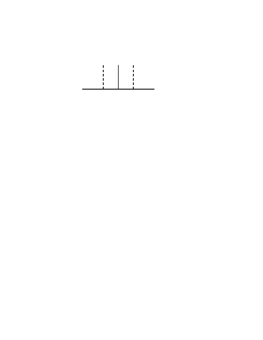
4.4 Lax-Phillips semigroup
49
..........
.
.
.
.
.
.
.
.
.
.
.
.
.
.
.
.
.
.
.
.
.
.
.
.
.
.
.
.
.
.
.
.
.
.
.
.
.
.
.
.
.
.
.
.
.
.
.
.
.
.
.
s
.
.
.
.
.
.
.
.
.
.
.
.
.
.
.
.
.
.
.
.
.
.
.
.
.
.
.
.
.
.
.
.
.
.
.
.
..
.
.........
............
..............................
...........
.
.
.
.
.
.
.
.
.
.
.
.
..
.
.
.
.
..
.
.
.
ω
.....
..................
...........
.
.
...........
.
..........
..
.
t
−R
R
.
.
.
.
.
.
.
.
.
.
.
.
.
.
.
.
Fig. 6. The Lax-Phillips semigroup
4.4 Lax-Phillips semigroup
In Section 3.4, I have already mentioned that the Lax-Phillips transform,
for odd dimensions, gives an isomorphism of the finite energy space
H
FE
(R
n
) to L
2
(R× S
n−1
) and intertwines the free wave group and the
translation group. Moreover for a potential perturbation the wave group
is conjugated to a group of bounded operators on L
2
(R×S
n−1
) satisfying
(3.33). This means that
k ∈ L
2
([−R, R] × S
n−1
) ⊂ L
2
(R× S
n−1
)
=⇒ W
V
(t)k = 0 in s < −R for t > 0.
(4.20)
This allows the Lax-Phillips semigroup to be defined by orthogonal pro-
jection onto L
2
([−R, R] × S
n−1
)
8
Z
V
(t)k = W
V
(t)k
¯
[−R, R] × S
n−1
, k ∈ L
2
([−R, R] × S
n−1
), t ≥ 0.
(4.21)
As the name suggests, this is a semigroup, Z(t)Z(s) = Z(t + s), for
t, s ≥ 0. Its infinitesimal generator
9
is
Z
V
(t) = exp(itL
V
), L
V
= D
s
+ V
LP
with domain
Dom(L
V
) =
k ∈L
2
([−R, R] × S
n−1
);
D
s
k ∈ L
2
([−R, R] × S
n−1
) and k(−R, ·) = 0
,
(4.22)
with V
LP
as described in Footnote 3.29.
8
That is, restriction back to [−R, R] × S
n−1
.
9
Existence of which is guaranteed by the Hille-Yosida theorem.

50
Trace formulæ and scattering poles
Lemma 4.2
For any odd n and V ∈ ˙C
∞
(B(R)) the infinitesimal gen-
erator of the Lax-Phillips semigroup has resolvent (L
V
− λ)
−1
, a mero-
morphic function of λ ∈ C with values in the bounded operators on
L
2
([−R, R] × S
n−1
) with poles of finite rank at precisely the poles of the
resolvent R(λ) and with the same multiplicities.
10
The proof of (4.19) uses this result. For t > 2R the Lax-Phillips
semigroup Z(t) is smoothing, and hence trace class as an operator on
L
2
([−R, R] × S
n−1
). Its trace is τ
V
(t) and its non-zero eigenvalues are
exp(iλt) for λ ∈ D(V ). In fact, for T > 0, a subspace of L
2
([−R, R] ×
S
n−1
) can be constructed on which the operator Z
V
(t) has, for t > T,
the same eigenvalues as it has on L
2
([−R, R] × S
n−1
) and on which it is
of trace class. Lidskii’s theorem, expressing the trace as the sum of the
eigenvalues then gives (4.19).
I give another application of the Lax-Phillips semigroup in Section 4.6
below.
4.5 Counting function
Discussion of the convergence of the right side of (4.19), as with (4.3), is
related to counting functions for the poles. In the odd-dimensional case
I shall simply consider the counting function
N (R) =
X
(λ,k)∈D(V ),|λ|≤R
k,
(4.23)
just the number of poles with absolute value less than R, as always
counted with multiplicity. The corresponding function for the case of
a compact manifold without boundary, see Footnote 1, has a leading
asymptotic term known as ‘Weyl’s law’ which is
11
N (R) = c
n
Vol(M )R
n
+ O(R
n−1
), n = dim M, for M compact.
(4.24)
For scattering by a potential there is, in odd dimensions, a similar upper
bound.
Proposition 4.4
If n ≥ 3 is odd and V ∈ C
∞
c
(R
n
) then
N (R) ≤ C + CR
n
.
(4.25)
10
So giving the same divisor.
11
See [19].

4.5 Counting function
51
This result is due to Zworski, [118], and is shown to be optimal by an
example in [119].
12
Zworski’s argument to get the precise order (4.25),
is a clever modification of the approach in [70]; it has been further sim-
plified and extended by Vodev ([116]). Such bounds are obtained by
showing that the poles are among the zeros of an entire function. As dis-
cussed in Lecture 2 the poles of the resolvent are the values of λ for which
the Lipmann-Schwinger operator Id +V R
0
(λ) is not invertible as an op-
erator on L
2
(B(R)). Since V R
0
(λ) is compact this is the same as the
values of λ for which −1 is an eigenvalue of V R
0
(λ). For k ≥
1
2
(n+1) the
product (V R
0
(λ))
k
is trace class so the non-invertibility of Id +V R
0
(λ),
which implies the non-invertibility of Id +(V R
0
(λ))
k
, means that the
Fredholm determinant
h
(k)
V
(λ) = det Id +(V R
0
(λ))
k
(4.26)
must have a zero at that point. This remains true with multiplicities
included, so to get an upper bound on the number of poles it suffices
to count the zeros of the entire function h
(k)
V
(λ). For an entire func-
tion Jensen’s inequality allows the counting function for the zeros to
be bounded in terms of the growth of the function itself. In particular
(4.25) follows from the estimate
|h
(n+1)
V
(λ)| ≤ Ce
C|λ|
n
.
(4.27)
Estimates due to Weyl allow the determinant in (4.26) to be bounded
in terms of the characteristic values of the operator A = (V R
0
(λ))
n+1
:
| det(Id +A)| ≤
∞
Y
j=0
(1 + χ
j
(A))
(4.28)
where the χ
j
(A) > 0 are positive square-roots of the eigenvalues of
A
∗
A, repeated with multiplicity. If H
R
is the characteristic function of
a ball of radius R, containing the support of V then V H
R
= V. The
characteristic values of a product satisfy
χ
j
(AB) = χ
j
(BA),
χ
j+k
(AB) ≤ χ
j
(A)χ
k
(B) and
χ
j
(AB) ≤ kAkχ
j
(B).
(4.29)
so it suffices to consider the characteristic values of H
R
R
0
(λ)H
R
, in
which V no longer appears explicitly. In the physical half-space, Im λ <
12
With n replaced by some integer this was proved in [70] and later improved to
n + 1 in an unpublished note.

52
Trace formulæ and scattering poles
0, the characteristic values of H
R
R
0
(λ)H
R
, are easily estimated uni-
formly and satisfy:
χ
j
(H
R
R
0
(λ)H
R
) ≤ Cj
−
1
n
, Im λ ≤ 0,
(4.30)
It follows that
13
χ
j(n+1)
((V R
0
(λ))
n+1
) ≤ C(χ
j
(H
R
R
0
(λ)H
R
))
n+1
=⇒ |h
(n+1)
V
| ≤ C in Im λ ≤ 0.
(4.31)
To estimate the characteristic values of H
R
R
0
(λ)H
R
in Im λ ≥ 0 the
identity (1.32) can be used. This allows the difference of the free resol-
vent at λ and −λ to be written
H
R
(R
0
(λ) − R
0
(−λ)) H
R
= iG
R
(λ)G
∗
R
(λ)
(4.32)
where G
R
: L
2
(S
n−1
) −→ L
2
(B(R)). The non-zero eigenvalues of G
R
G
∗
R
are the same as those of G
∗
R
G
R
which is an operator on L
2
(S
n−1
). Thus
it suffices to estimate, uniformly in λ, the characteristic values of the
operator, Q
R
, with Schwartz’ kernel
Q
R
(ω, τ, λ) =
Z
B(R)
e
iλ(ω−θ)·z
dz ∈ C
∞
(S
n−1
× S
n−1
).
(4.33)
This kernel is in fact real-analytic
14
and this leads to the uniform esti-
mates
χ
j
(H
R
R
0
(λ)H
R
) ≤
(
C exp 2T | Im λ|
for j ≤ C|λ|
n−1
Cj
−
1
n
for j > C|λ|
n−1
.
(4.35)
This gives (4.27) for all λ ∈ C and hence (4.25).
As already noted, (4.25) is optimal, in the sense that there are exam-
ples with this growth. In general no lower bound is known
15
The only
general lower bound for potential scattering of which I am aware arises
from the argument of Lax and Phillips for obstacle scattering [52], which
can be adapted to show
13
For various constants, C.
14
The norm, on L
2
(S
n−1
), of Q
p,R
= (∆
S n−1
+ 1)
p
Q
R
is, for some constant C
which is independent of p and λ, bounded by C
p
(1 + |λ|
2p
) exp(2R| Im λ|) Since
Q
R
= (∆
S n−1
+ 1)
−p
Q
p,R
this leads to bounds on the characteristic values in
terms of the eigenvalues of the Laplacian on the sphere:
χ
j
(Q
R
) ≤ j
−p
1
n−1
(C
′
)
p
(1 + |λ|
2p
) exp(2R| Im λ|).
(4.34)
Taking the minimum over p of the right side, for each fixed j gives (4.35).
15
Corollary 4.1 shows that for n = 3 and any potential, other than 0, there is
an infinite set of poles. The corresponding result is not known to hold in odd
dimensions n ≥ 5, or in any even dimension.

4.6 Pole-free regions
53
Lemma 4.3
For n = 3 and any potential V ∈ C
∞
c
(R
n
) of fixed sign, not
identically zero, the number of pure-imaginary poles satisfies
N
Im
(R) =
X
(is,k)∈D(V ),s∈[−R,R]
k ≥ cR
n−1
, c > 0.
(4.36)
For the even-dimensional case bounds on the number of poles have
been given by [46] and improved by Vodev ([114]) to
N (R, a) =
X
(λ,k)∈D(V ),|λ|≤R,
−a≤arg λ≤a
k
N (R, a) ≤ Ca (R
n
+ (log a)
n
) , a, R > 1
(4.37)
where, as usual, λ ∈ Λ is described formally by extension of the argument
to −∞ < arg λ < ∞.
4.6 Pole-free regions
There are only a finite number of poles of the analytic continuation of
the resolvent in the physical region, Im λ ≤ 0. In the odd-dimensional
case this can be extended to give pole free regions, near infinity, in which
Im λ → ∞ :
Proposition 4.5
For n ≥ 3 odd and any V ∈ C
∞
c
(R
n
), real-valued,
and any constant N there are only finitely many poles of the resolvent
satisfying
Im λ ≤ N + N log(1 + | Re λ|).
(4.38)
Results of this type were obtained by Lax and Phillips, [53], but for a
fixed N. The general estimate, (4.38), follows from the fact that for t >
2R the Lax-Phillips semigroup, Z
V
(t), has a C
∞
kernel as an operator
on [−R, R] × S
n−1
and depends smoothly on t. Thus the t-derivative of
any order, D
p
t
Z(t), is bounded for any p. The eigenvalues are therefore
bounded and thus
|λ
j
|
p
exp(−T Im λ
j
) ≤ C
p,T
(4.39)
holds for all j. This implies (4.38).

5
Obstacle scattering
So far I have considered, in the main, scattering theory for potential
perturbations of the flat Laplacian. In this lecture I wish to discuss
some of the properties of the more substantial perturbation obtained by
introducing a boundary in a compact region; in the last three lectures
I shall consider various problems which are not perturbations of Eu-
clidian space at all. Even restricting attention to compactly-supported
perturbations of Euclidian space, one can consider much more general
situations. For example the metric can be changed on a compact set,
1
the topology itself can be modified or the Laplacian can be deformed
in more serious ways, say to a hypoelliptic operator.
2
Rather generally
one can consider a ‘black box’ perturbation
3
with appropriate analytic
properties, and still variants of many of the results discussed below re-
main valid. Nevertheless it is worthwhile considering the different types
of perturbations separately, since they each have their own special fea-
tures. Even the subject of scattering by an obstacle is a large, and in
parts quite technical, one to which I cannot do justice in one lecture.
I shall therefore limit myself to discussing some representative results
which indicate both the similarities to, and differences from, the case of
potential scattering.
1
Such perturbations are included as a ‘trivial case’ in the discussion in Lecture 6.
2
For example it is only in cases like this, where the ‘spectral density’ is higher for
the perturbation than for the free problem that a leading asymptotic term for the
counting functions for the poles has been shown to exist – see [109] and for related
results [115] and [89].
3
For example, the analytic continuation of the resolvent for such general perturba-
tions is discussed by Sj¨
ostrand and Zworski in [108].
54

5.1 Obstacles
55
5.1 Obstacles
Consider a smooth ‘obstacle.’ This can be specified by a smooth compact
embedded (but not necessarily connected) hypersurface H ⊂ R
n
such
that
R
n
\ H = Ω ∪ O, with O compact and Ω connected
(5.1)
and with both O and Ω open. Thus O = O ∪ H is the ‘obstacle’ and
Ω is its exterior. On the boundary, H, of Ω a self-adjoint boundary
condition, such as the Dirichlet, Neumann or Robin condition, should
be specified for the Laplacian; for the sake of definiteness I shall only
consider the Dirichlet condition.
Using methods similar to those already described in the case of a
potential it follows that:
4
Proposition 5.1
For each 0 6= λ ∈ R and each ω ∈ S
n−1
there is a
unique function u ∈ C
∞
(Ω) satisfying (∆
− λ
2
)u = 0 in Ω and such that
u = e
iλz·ω
+ u
′
, u
′
= e
−iλ|z|
|z|
−
1
2
(n−1)
g(
z
|z|
) + u
′′
, u
′′
∈ L
2
(Ω)
(5.2)
where u = 0 on H and g ∈ C
∞
(S
n−1
).
This can be seen from the analytic continuation of the resolvent (∆ −
λ
2
)
−1
. As for potential scattering this operator, which is bounded on
L
2
(Ω) for λ in the physical space, the lower half-plane, continues ana-
lytically to an operator mapping C
∞
c
(Ω) to
C
∞
(Ω) and depending mero-
morphically on λ ∈ C or λ ∈ Λ according to the parity of the dimension.
5
For scattering by an obstacle there are no bound states, the only spec-
trum is [0, ∞) with no embedded eigenvalues.
6
4
This result, for odd dimensions, is contained, for example, in the book of Lax and
Phillips, [51].
5
The general strategy for proving such a result is to find a parametrix, i.e. an
inverse for the problem (which should be holomorphic in λ ∈ C or Λ, or at least
an arbitrarily large open subset), up to a compact error term. For potential
scattering the resolvent of the free Laplacian gives such a parametrix. For an
obstacle problem the theory of elliptic boundary problems (see for example [44])
gives a local parametrix for the boundary problem. This can be combined, using a
partition of unity, with the free resolvent near infinity to give a global parametrix.
The assumptions on a ‘black box’ perturbation should be made so that this type of
construction can be applied, see [108]. Once the parametrix has been constructed
arguments much as for potential scattering apply. For instance the resolvent of
the boundary problem can be related to that of the free problem, enough to give
Proposition 5.1.
6
The proof of the absence of embedded eigenvalues follows as in the potential case.

56
Obstacle scattering
Again as in the case of potential scattering it follows that, given 0 6=
λ ∈ R, for each g ∈ S(R
n
) and f ∈ C
∞
(S
n−1
) there is a unique solution
u ∈ C
∞
(Ω) of
(∆ − λ
2
)u = g in Ω satisfying v = 0 on H and
v = e
iλ|z|
|z|
−
1
2
(n−1)
f(
z
|z|
) + e
−iλ|z|
|z|
−
1
2
(n−1)
f
−
(
z
|z|
) + v
′
, v
′
∈ L
2
(Ω)
(5.3)
for some f
−
∈ C
∞
(S
n−1
). The generalized plane waves in Proposition 5.1
give a parametrization of the null space of the Laplacian on tempered
distributions (satisfying the boundary condition in a weak sense). The
solutions in (5.3) are dense in this space, and in fact there is a general-
ization where f ∈ C
−∞
(S
n−1
) which generates the whole null space. If
g ≡ 0 then f
−
is determined by f and the map
A
H
(λ) : f 7−→ f
−
(5.4)
is the absolute scattering matrix. From (5.2) and (1.13) it follows that
A
H
(λ)f(θ) = i
(n−1)
f(−θ) + (A
′
H
f)(−θ)
(5.5)
with A
′
H
a smoothing operator, i.e. of the form
A
′
H
f(θ) =
Z
S
n−1
A
′
H
(θ, ω, λ)f(ω)dω,
(5.6)
the (relative) scattering amplitude A
′
H
(θ, ω, λ) being a smooth function
of θ, ω ∈ S
n−1
for each 0 6= λ ∈ R.
7
Again as in the potential case
8
f and f
+
≡ 0 in (5.3) =⇒ v ∈ S(Ω);
f and f
+
≡ 0 and g ∈ C
∞
c
(R
n
) =⇒ v ∈ C
∞
c
(Ω).
(5.7)
It is also the case that no two different obstacles can have the same
scattering matrix.
Proposition 5.2
9
If n ≥ 3 is odd and H
i
, i = 1, 2 are two smooth
That there are no bound states is a consequence of the formal positivity of the
Laplacian with Dirichlet (or Neumann) boundary condition.
7
In fact it is real-analytic.
8
Indeed the proof reduces to the free case. Choose a function φ ∈ C
∞
c
(R
n
) which
is equal to 1 in a ball containing H in its interior. Then consider v
′
= (1 − φ)v,
it satisfies (∆ − λ
2
)v
′
∈ S(R
n
) and has the same asymptotic expansion as in
(5.3). Thus f ≡ f
+
≡ 0 implies v
′
∈ S(R
n
) and hence v ∈ S(R
n
). Similarly if
g ∈ C
∞
c
(R
n
) as well then v
′
must have compact support.
9
This result can be found as Theorem 5.6 of Chapter 5 of [51], where the proof
is attributed to Schiffer. For the given f ∈ C
∞
(S
n−1
) consider the solutions v
i
,
i = 1, 2, to (5.3) with g ≡ 0 for the two obstacles with boundaries H
i
. Using a

5.2 Scattering operator
57
embedded hypersurfaces as above then A
H
1
f = A
H
2
f for any one f ∈
C
∞
(S
n−1
),
10
not identically zero, for all 0 6= λ ∈ R implies H
1
= H
2
.
5.2 Scattering operator
Proposition 5.2 is an (older) analogue of Proposition 3.5 and is similarly
non-constructive, i.e. does not give a procedure by which H can be
recovered from A
′
H
. In search of a more constructive recovery procedure
consider the absolute scattering kernel
B
H
(t, θ, ω) =
1
2π
Z
R
e
−iλt
A
H
(θ, ω, λ)dλ
(5.8)
and the corresponding relative scattering kernel which is given by
B
′
H
(t, θ, ω) = i
n−1
(B
V
(t, −θ, ω) − δ(t)δ
ω
(ω).
These are both distributions in the space C
−∞
(R× S
n−1
× S
n−1
) with
the support property
H ⊂ {|z| ≤ R} =⇒ supp(B
′
H
) ⊂ {t ≥ −2R}.
(5.9)
The scattering operator is the operator on R× S
n−1
defined by B
H
,
or δ(t)δ
ω
(θ) + B
′
H
acting as a convolution operators in the t variable.
The most immediate invariants of such an operator are the singularities
of the kernel.
For the case of potential scattering it follows from the construction of
perturbed travelling wave solutions to the wave equation that
sing supp(B
′
V
) ⊂ {t = 0, θ = ω}.
(5.10)
In fact more is true. Not only is the singular support of B
′
V
contained
cutoff as in Footnote 8 it follows that v
1
− v
2
has compact support. By unique
continuation for elements of the null space of ∆ − λ
2
it follows that v
1
− v
2
must
vanish on the complement of O
1
∪ O
2
and hence on its boundary. If H
1
6= H
2
then, by relabelling it can be supposed that Ω
2
\ O
1
6= ∅. Consider any component
of Ω
2
\ O
1
. The boundary of such an open set is contained in the union of the
boundaries of O
1
and of the boundary of O
1
∪ O
2
. In either case v
2
must vanish
there, so v
2
is an eigenfunction, with Dirichlet boundary condition in this set.
Since the Dirichlet spectrum on any bounded open set has a positive lower bound,
it follows that for λ small enough v
2
≡ 0 in such an open set. However v
2
is
real-analytic in Ω
2
so this implies v
2
≡ 0 in Ω
2
. This contradiction implies that
H
1
= H
2
.
10
The same argument works if f ∈ C
−∞
(S
n−1
) and in particular if f is taken to be
the delta measure at some point ω then the identity of the two scattering matrices
for all θ ∈ S
n−1
and for all λ and one ω implies that H
1
= H
2
.

58
Obstacle scattering
in the ‘diagonal’ but, acting as a convolution operator in t :
B
′
V
∗ f(t, θ) =
∞
Z
−∞
Z
S
n−1
B
′
V
(t − t
′
, θ, ω)f(t
′
, ω)dωdt
′
,
(5.11)
B
′
V
is a pseudodifferential operator. More precisely, the wavefront set of
the scattering kernel satisfies
WF(B
′
V
) ⊂ {(0, ω, ω;τ, τ w, −τ w) ∈ T
∗
(R× S
n−1
× S
n−1
);
τ 6= 0 and ∃ z ∈ supp(V ) with (z − w) ⊥ ω}.
(5.12)
Thus the singularities of B
′
V
can be attributed to the geodesics which
pass through the support of V. Now, a geodesic in R
n
is a curve of the
form
z(t) = w
′
+ (t − t
′
)ω
′
, ω
′
∈ S
n−1
(5.13)
where w
′
and ω
′
are uniquely determined if it is required that w
′
·ω
′
= 0.
The geodesic passes through supp(V ) if z = w
′
+ t
′′
ω
′
∈ supp(V ) for
some t
′′
, i.e. w
′
is in the projection of supp(V ) into the plane orthogonal
to ω. For each 0 6= τ ∈ R, this gives a point in the set on the right in
(5.12) and every such point arises this way.
5.3 Reflected geodesics
To generalize (5.12) to obstacle scattering the notion of a reflected
geodesic is needed. I shall consider only ‘C
∞
’ geodesics,
11
those which
are related to the propagation of singularities in the C
∞
sense. A re-
flected geodesic is a curve I ∋ t −→ z(t) ∈ Ω, where I ⊂ R is an interval,
which satisfies a condition near each point, depending on the nature of
the point. A curve is admitted as a reflected geodesic if it satisfies one
of the following conditions near each point z(t
′
) :
12
(i) z(t
′
) ∈ Ω and z(t) is a free geodesic nearby.
Thus z(t) is in the interior nearby and the curve is a straight line segment
as in (5.13), for |t − t
′
| < ǫ for some ǫ > 0.
(ii) z(t
′
) ∈ H with transversal, equal-angle reflection.
11
Note that the ‘C
∞
’ definitely refers to the space of functions modulo which the
singularities travelling along the curves are computed, not the curves themselves
which are not even C
1
in general.
12
Of course t ∈ I throughout.

5.3 Reflected geodesics
59
......
......
......
......
.....
......
.....
......
......
......
......
......
.......
.......
.......
........
.........
.........
............
............
..............
..............................................................
..........
...........
............
................
.....................
....................................
........
.......
.......
......
......
......
......
......
......
......
.....
......
.....
......
.....
......
.....
......
......
......
......
......
......
.......
.......
.......
..........
...................................
............
...........
............
...........
..........
............
..........
..........
..........
..........
...........
...........
..........
..
...........
...........
...........
.
..........
.
..........
.
...........
.
..........
..........
..
..
.
..........
..
..
.
..........
..
..
.
..
.
..
.
.
..
.
.
.
.
.
.
.
.
.
.
.
.
.
.
.
.
.
.
.
.
.
.
.
.
.
.
.
.
.
.
.
.
.
.
.
.
.
.
.
.
.
.
.
.
.
.
.
.
.
.
.
.
.
.
.
.
.
.
.
.
.
.
.
.
.
.
.
.
.
.
.
.
.
.
.
.
.
.
.
.
.
.
.
.
.
.
.
.
.
.
.
.
.
.
.
.
.
.
.
.
.
.
.
.
.
.
.
.
.
.
.
.
.
.
.
.
.
.
.
.
.
.
.
.
.
.
.
.
.
.
.
.
.
.
.
.
.
.
.
.
.
.
.
.
.
.
.
.
.
.
.
.
.
.
.
.
.
.
.
.
.
.
.
.
.
.
.
.
.
.
.
.
.
.
.
.
.
.
.
.
.
.
.
.
.
.
.
.
.
.
.
.
.
.
.
.
.
.
.
.
.
.
.
.
.
.
.
.
.
.
.
.
.
.
.
.
.
.
.
.
.
.
.
.
.
.
.
.
.
.
.
.
.
.
.
.
.
.
.
.
.
.
.
.
.
.
.
.
.
.
.
.
.
.
.
.
.
.
.
.
.
.
.
.
.
.
.
.
.
.
.
.
.
.
.
.
.
.
.
.
.
.
.
.
.
.
.
.
.
.
.
.
.
.
.
.
.
.
..
.
.
.
.
.
.
.
.
.
.
.
.
.
.
.
.
.
.
.
.
.
.
.
.
.
.
.
.
.
.
.
.
.
.
.
.
.
.
.
.
.
.
.
..
.
.
..
.
..
.
..
..
...
...
..
...
...
..
...
....
...
....
....
.....
.....
.....
...
....
........
.
.
.
.
.
.
.
.
.
.
.
.
.
.
.
.
.
.
.
.
.
.
.
.
.
.
.
.
.
.
.
.
.
.
.
.
.
.
.
.
.
.
.
.
.
.
.
.
.
.
.
.
.
.
.
.
.........
......
......
......
.
.........
........
.......
..
.....
..............
...........
...
.
..
.
.
..
.
...
..
.
..........
.
.
.............
.
.
.
.
.
.
.
.
..
.
.
.
.
.
.
..
.
.
......
....
......
.....
...
..
......
.......
.......
......
.......
......
......
.......
......
.......
......
............
.
............
.
...........
..
............
.
............
.
......
(ii)
(iii)
(v)
(v)
(iv’)
O
Ω
......
......
.
......
......
.
......
......
.
......
......
.
.
..
.
..
..
..
.
..
..
..
..
.
..
..
..
..
.
..
..
..
..
.
.
.
..
..
..
.
..
..
.
.
..
.
..
..
..
.
..
..
..
..
.
..
..
..
Fig. 7. Reflected geodesics.
By this I mean that if ν is the unit inward-pointing (with respect to Ω)
normal to H at z(t
′
) then there are two directions ω
′
, ω
′′
∈ S
n−1
such
that ω
′′
− ω
′
= cν, c > 0, and for some ǫ > 0, z(t) = z(t
′
) + (t − t
′
)ω
′
,
for t
′
− ǫ < t < t
′
, and z(t) = z(t
′
) + (t − t
′
)ω
′′
for t
′
< t < t
′
+ ǫ. This
is Snell’s law.
(iii) z(t
′
) ∈ H and z(t) is a diffractive ray nearby.
This means that for some ω ∈ S
n−1
with ω · ν = 0, and some ǫ > 0,
z(t) = z(t
′
) + (t − t
′
)ω where the ω-directional curvature of H, with
respect to Ω is strictly negative at z(t
′
).
13
(iv) z(t
′
) ∈ H, z(t) − z(t
′
) − (t − t
′
)ω = O(|t − t
′
|
3
2
) with ω · ν = 0
and the ω-directional curvature is non-negative at z(t
′
).
This is the residual case and can naturally be divided into two. If the
ω-directional curvature is strictly positive at z(t
′
) then it is necessarily
positive nearby. It can then be shown that
(iv’) z(t
′
) ∈ H and z(t) is a gliding ray nearby.
This means that z(t) ∈ H for |t − t
′
| < ǫ and z(t) is a geodesic for the
induced Riemann structure on H. This leaves only the cases of ‘higher
order contact:’
13
The directional curvature is the curvature of the curve formed by H ∩ P as a curve
in the 2-plane P = sp{xν + yω} where ν is the unit normal as before.

60
Obstacle scattering
..........
.
..........
.
..........
..........
..
..........
..........
.
..........
..
..
..........
.
...
..
..
.
...
..
.
.
..
.
.
..
.
.
.
.
.
.
.
.
.
.
.
.
.
.
.
.
.
.
.
.
.
.
.
.
.
.
.
.
.
.
.
.
.
.
.
.
.
.
.
.
.
.
.
.
.
.
.
.
.
.
.
.
.
.
.
.
.
.
.
.
.
.
.
.
.
.
.
.
.
.
.
.
.
.
.
.
.
.
.
.
.
.
.
.
.
.
.
.
.
.
.
.
.
.
.
.
.
.
.
.
.
......
......
......
......
......
......
......
......
......
......
......
......
......
......
......
......
......
......
......
.......
........
.............
......................................................................
..........
.
..
...........
.
.
.
...........
.
...........
..
..
...........
.
.
.
.
.
.
.
.
.
.
.
.
.
.
.
.
.
.
.
.
.
.
.
.
.
.
.
.
.
.
.
.
.
.
.
.
.
.
.
.
O
Ω
Fig. 8. Non-uniqueness of extension of reflected geodesics.
(v) z(t
′
) ∈ H, z(t) − z(t
′
) − (t − t
′
)ω = O(|t − t
′
|
3
2
) with ω · ν = 0
and the ω-directional curvature is zero at z(t
′
).
As with geodesics on a complete manifold, such as R
n
, these reflected
geodesics can be continued indefinitely in each direction. However in
general there is no uniqueness for the continuation. Non-uniqueness can
occur only at points at which the directional curvature vanishes to infi-
nite order. If the boundary H is real-analytic there is always uniqueness.
The following example of non-uniqueness of the continuation of rays is
due to Taylor ([112].)
Example
Consider a region in the plane bounded by a curve on which
there is a point at which the curvature vanishes to infinite order but at
which it has a simple change of sign, i.e. it is negative on one side and
positive on the other. There is then a straightline segment in Ω which is
tangent to the boundary, to infinite order, at the flat point; see Figure 8.
This segment lies on the side on which the obstacle is locally convex. It
is possible to arrange that, on the side of the curve on which the obstacle
is concave, there is a ray which is reflected infinitely often with a limit
point at the point of vanishing curvature.
14
It is straightforward to
check that, together, the free segment and the infinitely reflected curve
form a reflected ray according to the definition above. However, it is
14
Draw in the infinitely reflected ray first by taking a sequence of intervals, the sum
of the lengths of which converges, and arrange them end to end with successive
angle changes which are all of fixed sign and are small compared to the lengths
(i.e. the angles tend to zero when divided by any fixed power of the length. Then
it is easy to show that a curve can be drawn through the points of reflection so
that Snell’s law holds and the curvature has the stated properties.

5.4 Ray relation
61
also the case that the free segment together with the boundary curve in
the concave region constitutes a reflected ray. This shows that there is
non-uniqueness for the local continuation of the incoming free segment,
as a ray.
15
5.4 Ray relation
For each ω ∈ S
n−1
and each w ∈ R
n
with w · ω = 0 there is a ray coming
in from infinity:
z(t) = w + tω, t << 0.
(5.14)
This can be continued, possibly in more than one way. The ray will strike
the obstacle if w lies in the projection of the obstacle in the direction ω.
If the obstacle is contained in the ball |z| ≤ R and a continuation of the
ray leaves this ball then it will be of the form
z(t) = w
′
+ (t − t
′
)ω
′
, ω
′
∈ S
n−1
for t >> 0
(5.15)
where again w
′
· ω
′
= 0. The ray relation of the obstacle is the set
Λ
H
= {(t
′
, ω
′
, ω, τ, τ w
′
, −τ w); 0 6= τ ∈ R}
(5.16)
where there is a ray z(t) of the form (5.14) and (5.15). The value of t
′
for a particular point in the ray relation is called the sojourn time of
that ray.
16
It is a measure of the ‘additional time’ the ray spends in the
neighbourhood of the obstacle. The regular part of the ray relation is
defined by
Λ
reg
H
=
(t
′
, ω
′
, ω, τ, τ w
′
, −τ w); 0 6= τ ∈ R
and there is no point of the type (iii) or (v) on the ray
.
(5.17)
The rays defining Λ
reg
H
are actually those which do not have any point
of type (iii) or (iv), since a point of type (iv’) cannot occur until one of
type (v) has been encountered. The transversality of the reflection at
points of type (ii) means that Λ
reg
H
is a smooth submanifold.
17
15
In fact it can be shown, using the dynamical properties of rays, that the set of
points which can be reached at a fixed distance along all the continuations of any
one ray, is always connected. Thus in this case there must be an uncountably
infinite set of continuations of the given ray!
16
This concept was introduced by Guillemin in [29] which was the first systematic
application of microlocal analysis to scattering theory. It is still very much worth
reading.
17
I conjecture, having not seen an explicit proof, that Λ
reg
H
is
precisely the smooth
part of Λ
H
.

62
Obstacle scattering
The fibre of the cotangent bundle of the sphere, T
∗
S
n−1
, at the point
ω can be identified with the orthocomplement of ω in R
n
. Since T
∗
(R×
S
n−1
× S
n−1
) is isomorphic to T
∗
R
× T
∗
S
n−1
× T
∗
S
n−1
the ray relation
can be identified as a subset of the cotangent bundle of R×S
n−1
×S
n−1
.
The regular part is a Lagrangian submanifold.
18
Proposition 5.3
19
The scattering kernel for an obstacle satisfies
Λ
reg
H
⊂ WF(B
H
) ⊂ Λ
H
.
(5.18)
Given the conjecture in Footnote 17 this means that the regular set
Λ
reg
H
can be recovered from B
′
H
; indeed it can be recovered from the
knowledge of B
′
H
modulo C
∞
terms. In any case the closure of Λ
reg
H
can be recovered from the wavefront set, since the complementary part
has smaller Hausdorff dimension.
20
One can therefore ask the natural
question as to whether Λ
reg
H
determines H. That this is not the case
is shown by the following example due to Livshits
21
, see also the note
of Rauch [97] and related examples given by Penrose in a somewhat
different context.
Example
Consider the obstacle in Figure 9. The inner curve between
A and B is part of an ellipse, including the half above the major semi-
axis, CD; E and F are the foci of this ellipse. The boundary curve is
simply tangent to the major semiaxis at E and F and is otherwise just a
smooth, say C
∞
, curve, H, which does not meet the major semiaxis CD
at any other point. This forms the boundary of the obstacle O. Consider
the behaviour of reflected (C
∞
) rays for this obstacle. Any ray passing
18
That is the symplectic form vanishes when restricted to Λ
reg
H
.
19
The first inclusion follows from the fact that B
′
H
is a Lagrangian distribution,
microlocally near Λ
reg
H
. That is, it can be constructed quite explicitly in terms
of oscillatory integrals. The second inclusion follows from a construction as in
Section 3.5 which allows B
H
to be obtained as the Lax-Phillips transform of a
solution to the forcing problem (with Dirichlet boundary condition on O.) Results
on the propagation of singularities (by Taylor [112] and in [67], [79] and [80], see
also [44]) and the calculus of wavefront sets (using the properties of the Radon
transform as a Fourier integral operator) then lead to (5.18). Unfortunately I do
not know of anywhere this is published in full detail.
20
That is, the closure of Λ
reg
H
is necessarily the closure of the subset of WF(B
H
)
which is a smooth manifold of dimension n + 1. This also suggests some more
geometric questions. Since WF(B
H
) is closed, the closure of Λ
reg
H
is also a subset
of Λ
H
. Is it the case that Λ
H
= Λ
reg
H
? It seems to me that this should be true. It
would imply that
WF(B
H
) = Λ
H
.
(5.19)
21
Mikhail Livshits to be precise. Unfortunately this example was not published by
him.

5.4 Ray relation
63
......
...
....
....
..
...
..
..
..
..
.
..
.
..
.
..
.
.
.
..
.
.
.
.
..
.
.
.
.
.
.
.
.
.
.
.
.
.
.
.
.
.
.
.
.
.
.
.
.
.
.
.
.
.
.
.
.
.
.
.
.
.
.
.
.
.
.
.
.
.
.
.
.
.
.
.
.
.
.
.
.
.
.
.
.
.
.
.
.
.
.
.
.
.
.
.
.
.
.
.
.
.
.
.
.
.
.
.
.
.
.
.
.
.
.
.
.
.
.
.
.
.
.
.
.
.
.
.
.
.
.
.
.
.
.
.
.
.
.
.
.
.
.
.
.
.
.
.
.
.
.
.
.
.
.
.
.
.
.
.
.
.
.
.
.
.
.
.
.
.
.
.
.
.
.
.
.
.
.
.
.
.
.
.
.
.
.
.
.
.
.
.
.
.
.
.
.
.
.
.
.
.
.
.
.
.
.
.
.
.
.
.
.
.
.
.
.
.
.
.
.
.
.
.
.
.
.
.
.
.
.
.
.
.
.
.
.
.
.
.
.
.
.
.
.
.
.
.
.
.
.
.
.
.
.
.
.
.
.
.
.
.
.
.
.
.
.
.
.
.
.
.
.
.
.
.
.
.
.
.
.
.
.
.
.
.
.
.
.
.
.
.
.
.
.
.
.
.
.
.
.
.
.
.
.
.
.
.
.
.
.
.
.
.
.
.
.
.
.
.
.
.
.
.
.
.
.
.
.
.
.
.
.
.
.
.
.
.
.
.
.
.
.
.
.
.
.
.
.
.
.
.
.
.
.
.
.
.
.
.
.
.
.
.
.
.
.
.
.
.
.
.
.
.
.
.
.
.
.
.
.
.
.
.
.
.
.
.
...
.
.
.
.
...
.
...
.
...
..
..
.
...........
.
..........
.....
..........
..........
..
..........
.
.
..
.
...
.
.
..
.
.
.
.
...
.
.
.
.
.
.
.
.
.
.
.
.
.
.
..........
..........
..........
............
.............
..........
A
B
C
D
E
F
....
.....
....
.....
....
...
...
...
..
...
..
..
..
..
.
..
..
.
..
..
.
.
..
.
..
.
.
..
.
.
.
..
.
.
.
..
.
.
.
.
.
.
.
.
.
..
.
.
.
.
.
.
.
.
.
.
.
.
.
.
.
.
.
.
.
.
.
.
.
.
.
.
.
.
.
.
.
.
.
.
.
.
.
.
.
.
.
.
.
.
.
.
.
.
.
.
.
.
.
.
.
.
.
.
.
.
.
.
.
.
.
.
.
.
.
.
.
.
.
.
.
.
.
.
.
.
.
.
.
.
.
.
.
.
.
.
.
.
.
.
.
.
.
.
.
.
.
.
.
.
.
.
.
.
.
.
.
.
.
.
.
.
.
.
.
.
.
.
.
.
.
.
.
.
.
.
.
.
.
.
.
.
.
.
.
.
.
.
.
.
.
.
.
.
.
.
.
.
.
.
.
.
.
.
.
.
.
.
.
.
.
.
.
.
.
.
.
.
.
.
.
.
.
.
.
.
.
.
.
.
.
.
.
.
.
.
.
.
.
.
.
.
.
.
.
.
.
.
.
.
.
.
.
.
.
.
.
.
.
.
.
.
.
.
.
.
.
.
.
.
.
.
.
.
.
.
.
.
.
.
.
.
.
.
.
.
.
.
.
.
.
.
.
.
.
.
.
.
.
.
.
.
.
.
.
.
.
.
.
.
.
.
.
.
.
.
.
.
.
.
.
.
.
.
.
.
.
.
.
.
.
.
.
.
.
.
.
.
.
.
.
.
.
.
.
.
.
.
.
.
.
.
.
.
.
.
.
.
.
.
.
.
.
.
.
.
.
.
.
.
.
.
.
.
.
.
.
.
.
.
.
.
.
.
.
.
.
.
.
.
.
.
.
.
.
.
.
.
.
.
.
.
.
.
.
.
.
.
.
.
.
.
.
.
.
.
.
.
.
.
.
.
.
.
.
.
.
.
.
.
.
.
.
.
.
.
.
.
.
.
.
.
.
.
.
.
.
.
.
.
.
.
.
.
.
.
.
.
.
.
.
.
.
.
.
.
.
.
.
.
.
.
.
.
.
.
.
.
.
.
.
.
.
.
.
.
.
.
.
.
.
.
.
.
.
.
.
.
.
.
.
.
.
.
.
.
.
.
.
.
.
.
.
.
.
.
.
.
.
.
.
.
.
.
.
.
.
.
.
.
.
.
.
.
.
.
.
.
.
.
.
.
.
.
.
.
.
.
.
.
.
.
.
.
.
.
.
.
.
.
.
.
.
.
.
.
.
.
.
.
.
.
.
.
.
.
.
.
.
.
.
.
.
.
.
.
.
.
.
.
.
.
.
.
.
.
.
.
.
.
.
.
.
.
.
.
.
.
.
.
.
.
.
.
.
.
.
.
.
.
..
.
.
.
.
.
.
..
.
.
.
..
.
.
.
...
.
...
..
.
...
..........
.
...........
.
..........
.
..........
......
..........
..........
...........
..
..........
.
.
..........
.
...
..
.
.
..
.
.
.
..
.
.
.
..
.
.
.
.
.
.
.
.
.
...
.
.
.
.
.
.
.
.
.
.
.
.
.
.
.
.
.
.
.
.
.
.
.
.
.
.
.
.
.
.
.
.
.
.
.
.
.
.
.
.
.
.
.
.
.
.
.
.
.
.
.
.
.
.
.
.
.
.
.
.
.
.
.
.
.
.
.
.
.
.
.
.
.
.
.
.
.
.
.
.
.
.
.
.
.
.
.
.
.
.
.
.
.
.
.
.
.
.
.
.
.
.
.
.
.
.
.
.
.
.
.
.
.
.
.
.
.
.
.
.
.
.
.
.
.
.
.
.
.
.
.
.
.
.
.
.
.
.
.
.
.
..........
..........
...........
..........
...........
...........
............
.............
.............
.............
...............
................
..................
...................
.......................
.......................
O
Ω
......
.
.....
....
...
..
..
..
..
.
..
.
..
.
.
..
.
.
.
.
.
.
.
.
.
.
.
.
.
.
.
.
.
.
.
.
.
.
.
.
.
.
.
.
.
.
.
.
.
.
.
.
.
.
.
.
.
.
.
.
.
.
.
.
.
.
.
.
.
.
.
.
.
.
.
.
.
..
.
.
.
.
.
..
.
.
..
...
..
..
...........
..........
......
......
......
......
......
......
.......
........
...........
.................................
............
...........
...........
..........
.
.
.
.
.
.
.
.
.
.
.
.
.
.
.
.
.
.
.
.
.
.
.
.
.
.
.
.
.
.
.
.
.
.
.
.
.
.
.
.
.
.
.
.
.
.
.
.
.
.
..
.
..
..
.
.........................
....................
......
......
.
.
.
.
.
.
.
.
.
.
.
.
.
.
.
.
.
.
.
.
.
.
.
.
.
.
.
.
.
.
.
.
.
.
.
.
.
.
.
.
.
.
.
.
.
.
.
.
.
.
.
.
.
.
.
.
.
.
.
.
.
.
.
.
.
.
.
.
.
.
.
.
.
.
.
.
.
.
.
.
.
.
.
.
.
.
.
.
.
.
.
.
.
..
.
.
.
.
.
.
..
.
.
..
.
.
..
.
..
.
..
.
..
..
..
..
..
..
..
..
...
...
...
....
.....
......
.
.....
.....
.....
.....
.....
....
....
.................................................................
..............
...........
.........
........
........
.......
......
.......
......
......
......
.....
.....
.....
.....
...
.....
..
....
....
......
......
.
......
......
.
......
......
.
......
......
.
......
......
.
......
......
.
......
......
.
......
......
.
..
...
...
...
..
...
...
...
...
.
..
...
...
...
..
.
...
...
...
...
...
...
...
...
.
.
...
...
...
...
...
...
...
...
.
...........
..
.
..........
..
..........
.
..
.
..........
..
...........
.
.
..........
.
..
.
..........
..
..........
...
...........
..
..........
...
...........
..
..........
...
...........
..
..........
...
...........
..
Fig. 9. Two secret rooms
upward through the segment EF of the major semiaxis is immediately
reflected back again, across the same segment.
22
This means that any
reflected ray coming in from infinity cannot enter the region of O lying
below F D (or CE.) Thus, from the propagation of singularities result,
(5.18), and the stronger result that B
H
is determined microlocally by
the obstacle in a neighbourhood of the region accessible by rays com-
ing in from infinity, it follows that WF(B
H
), or even B
H
modulo C
∞
,
cannot detect the structure of the boundary in the open region DF (or
CE.) Thus by smoothly modifying the boundary near B one can get
two
23
different obstacles with scattering kernels which differ by a C
∞ 24
function.
25
22
This is the basic property of the ellipse, that the two lines to the foci from a
point on the ellipse make equal angles with the normal to the ellipse at that point.
Snell’s law then implies that the reflected ray from a point on EF also crosses EF.
23
Or even an uncountably infinite set of such obstacles.
24
Quite a lot is now known about the propagation of singularities modulo finer
regularity than C
∞
. In this case one would expect that, if the boundary is just
short of analytic, in the sense that it is in all Gevrey classes greater than 1 (the
obstacle can be constructed in these classes) then the singularities at the level of
Gevrey 3 or finer may well detect the difference between two such obstacles. For
a discussion of the propagation of Gevrey regularity see [55].
25
Notice that the ‘rooms’ bounded by F BD or CAE are ‘quiet’ (or ‘dark’) in the
sense that no strong waves can reach there from outside. On the other hand the
echo in there might be a bit strong.

64
Obstacle scattering
Despite this counterexample there are several positive results. If the
obstacle is convex then Λ
H
is the closure of Λ
reg
H
and the obstacle is
easily recovered from it. In fact Majda [56], see also [57], observed that,
assuming H to be smooth and convex, it can be recovered from the
backscattering; more precisely it can be recovered from the singularities
of B
H
¯
R
× ∆
−
(S
n−1
).
26
In fact the same is true if the obstacle is
normally accessible in the sense that the outward normal from each
point of H does not hit the obstacle at any other point.
5.5 Trapped rays
The global behaviour of the reflected geodesics, for instance if there are
periodic rays, has a very considerable effect on the scattering properties.
One natural condition, the importance of which was emphasized by Lax
and Phillips is
Definition 5.2
An obstacle is said to trap rays, or to have trapped rays,
if the sojourn time is unbounded above, i.e. for any T there is an element
of the ray relation (t
′
, ω
′
, ω, τ, τ w
′
, −τ w) with t
′
> T. If the obstacle does
not trap rays it is said to be ‘non-trapping.’
Thus if the obstacle is non-trapping, the singular support of the scat-
tering kernel is compact.
27
In odd dimensions the Lax-Phillips semi-
group can be defined very much as in the case of potential scattering
and the argument in Proposition 4.5 carries over to give
Proposition 5.4
If n ≥ 3 odd and the obstacle is non-trapping then
for any constant N there are only finitely many poles of the resolvent
satisfying
Im λ ≤ N + N log(1 + | Re λ|).
(5.20)
A question posed by Lax and Phillips concerns the possible converse to
Proposition 5.4. They had originally conjectured that an obstacle which
trapped rays would necessarily have a sequence of poles with imaginary
part tending to zero. This was shown not to be the case by Ikawa, see [45]
26
Here ∆
−
(S
n−1
) is the antidiagonal, where ω = −θ in S
n−1
× S
n−1
. It is also of
interest to note that the fact that the obstacle is convex can be determined from
the regular part of the ray relation. Namely the convexity of O is equivalent to
the fact that for every ω 6= θ there is a unique ray in Λ
reg
H
linking ω and θ.
27
This is true for example if the obstacle is star-shaped in the sense that there is a
fixed point p such that for each ω ∈ S
n−1
there is exactly one point on H of the
form p + r
ω
ω with r
ω
> 0.

5.5 Trapped rays
65
for a simple system of two disjoint convex obstacles. The existence and
position of ‘pseudo-poles’ for this problem had previously been shown
by Bardos, Guillot and Ralston [6] and the distribution of the poles has
been more precisely analyzed by G´erard in [26]. Nevertheless various
modified forms of the Lax-Phillips conjecture are consistent with present
knowledge of the distribution of poles in scattering theory. For example
Modified Lax-Phillips conjecture (A)
28
For every trapping obstacle there are infinitely many poles in some
half-space Im λ < C.
Modified Lax-Phillips conjecture (B)
For every trapping obstacle there are infinitely many poles in any
region Im λ ≤ N + N log(1 + | Re λ|).
29
The overall estimates on the distribution of poles are also the same as
in the case of potential scattering.
Proposition 5.5
For n ≥ 3 odd the counting function for scattering
poles, given by (4.23) satisfies (4.25)
30
.
Similarly the trace formula, (4.11) carries over directly
τ
H
(t) = F
−1
d
dλ
s
H
(λ)
(5.21)
where s
H
(λ) is −i times the logarithm of the determinant of the scat-
tering matrix.
31
From this a form of ‘Weyl’s law’ for the large frequency
behaviour of the scattering phase can be deduced:
s
H
(λ) = c
n
Vol(O)λ
n
+ O(λ
n−1
) as λ → ∞.
(5.22)
This is an analogue of (4.18) but there is no full asymptotic expansion
in case the obstacle is trapping.
32
The Poisson formula (4.19) is also valid for obstacle scattering.
33
This
has been used to get a variety of estimates on the distribution of scatter-
ing poles under various conditions. I will only discuss one such result
34
28
By assumption n ≥ 3 is odd always here.
29
Of course (A) implies (B)!
30
This is shown in [71]; this indeed was the first case in which the optimal order
bound was proved, even though the obstacle case is the more difficult technically.
31
So it doesn’t matter that this is only determined up to an additive constant.
32
The result is then rather harder to prove; see [72].
33
First proved for all t 6= 0 in [69]; see Sj¨
ostrand-Zworski [110] for a discussion
including ‘black-box’ perturbations in odd dimensions.
34
See Zworski’s survey [120] for a more complete discussion.

66
Obstacle scattering
Namely, consider a strictly convex obstacle. Harg´e and Lebeau, [34],
using the complex scaling method (similar to that used by Sj¨
ostrand and
Zworski in [109]) showed that the poles satisfy an estimate
35
Im λ > c| Re λ|
1
3
, c > 0.
(5.23)
They even give a geometrically determined value of c for which there are
at most a finite number of poles not satisfying (5.23).
35
A similar estimate on any real-analytic obstacle which is non-trapping for C
∞
rays was obtained by Bardos, Lebeau and Rauch [7], see also Popov [95], using
the results, on the propagation of singularities with respect to functions of Gevrey
class 3, by Lebeau [55].

6
Scattering metrics
In the last three lectures I shall stray beyond the confines of ‘traditional,’
i.e. Euclidean, scattering theory. I want to show how some of the ideas
and methods of Euclidean scattering can be extended to give a detailed
description of the generalized eigenfunctions of the Laplacian on certain
complete Riemannian manifolds with a regular structure at infinity. I
shall discuss, in varying levels of detail, five main classes of such met-
rics, each being a complete metric on the interior of a compact manifold
with boundary. The first two of these, consisting of asymptotically flat
(‘scattering’ or ‘sc-’) metrics and cylindrical end (‘boundary’ or simply
‘b-’) metrics will be the topics of this, and the penultimate, lecture. In
each case I will try to show that these classes of metrics exemplify a
general principle. Namely for each of them there are results analogous
to the standard differential-geometric theorems on a compact manifold
with boundary. These results include a ‘Hodge theorem’ (description of
the null space of the Laplacian on forms) a ‘Seeley theorem’ (description
of the resolvent family as pseudodifferential operators
1
) an ‘index theo-
rem’ (description of the Fredholm properties of these pseudodifferential
operators and
2
a formula of Atiyah-Singer type for the index). In the
final lecture I shall try to give an overview of the classification of these
metrics.
The class I shall talk about today consists of the scattering metrics.
These are direct generalizations of Euclidean spaces. Thus one can
expect that the results are rather direct extensions of those discussed
above. This is indeed the case, but the possibility of non-trivial topol-
1
Hence the possibility of describing the structure of functions of the operator, e.g.
complex powers, see [104] and [105].
2
At least in some cases!
67

68
Scattering metrics
ogy in the underlying space means that even some things which are
simple on Euclidean space manifest interest in the more general setting.
6.1 Manifolds with boundary
The setting for these metrics is an arbitrary compact manifold with
boundary, X.
3
The ‘trivial case’ to bear in mind is S
n
+
, obtained by
stereographic compactification of R
n
. The form of the Euclidean metric
on S
n
+
has already been discussed in (1.52). This can be generalized im-
mediately to any compact manifold with boundary. A Riemann metric
4
on X
◦
, the interior of X, is a scattering metric if it can be written in
the form
g =
dx
2
x
4
+
h
x
2
(6.1)
where h is a smooth symmetric 2-cotensor which is positive-definite when
restricted to the boundary
5
and x ∈ C
∞
(X) is a boundary defining
function.
6
In fact it is straightforward to check that, once it is known to
exist, the form (6.1) of the metric determines x ∈ C
∞
(X) up to addition
3
A manifold with boundary, by implication always C
∞
, is a Hausdorff and para-
compact topological space, X, which is locally modelled on a half space, R
n
+
=
[0, ∞) × R
n−1
. An open subset U ⊂ R
n
+
is the intersection of an open subset
U
′
⊂ R
n
with R
n
+
. A smooth function on U is, by definition, the restriction to
U of a element of C
∞
(U
′
) and the space of these functions is denoted C
∞
(U ).
Similarly a diffeomorphism between open sets of R
n
+
is taken to be the restriction
to these sets of a diffeomorphism between open subsets of R
n
. Then the C
∞
struc-
ture on X is given by a covering of X by open subsets U
j
each homeomorphic
to an open subset of
e
U
j
⊂ R
n
by maps f
j
: U
j
→
e
U
j
such that for each j, k
with U
j
∩ U
k
6= ∅ the composite map f
j
◦ f
−1
k
: f
k
(U
j
∩ U
k
) → f
j
(U
j
∩ U
k
) is a
diffeomorphism of open subsets of R
n
+
.
4
Meaning of course a positive-definite smooth 2-cotensor on X
◦
.
5
The tangent and cotangent bundles of a manifold with boundary are defined as
in the case of manifolds without boundary. In fact any manifold with boundary
can be ‘doubled’ across the boundary to a manifold without boundary, which I
will denote somewhat enigmatically as 2X. The tangent and cotangent bundles
are then naturally the restrictions to X of the bundles over the double. Thus h is
supposed to be a smooth section of T
∗
X ⊗ T
∗
X which is symmetric and smooth
up to the boundary in the sense that it is the restriction of a smooth section over
the double. The tangent bundle to the boundary is a smooth subbundle of the
restriction of T X to the boundary, which I denote T
∂X
X. Thus the condition that
h
∂X
∈ C
∞
(X; T
∗
X ⊗ T
∗
X) should restrict to a positive definite form on each
space T
p
∂X × T
p
∂X ⊂ T
p
X × T
p
X for p ∈ ∂X is meaningful.
6
Boundary defining functions always exist on a manifold with boundary, that is
there is always a function x ∈ C
∞
(X) which satisfies x ≥ 0, x = 0 on ∂X and
dx 6= 0 at ∂X. Any two boundary defining functions x and x
′
are related by
x
′
= ax where a ∈ C
∞
(X) is everywhere positive.

6.2 Hodge theorem
69
of a smooth multiple
7
of x
2
and hence fixes h
∂X
unambiguously. Thus
the boundary ∂X is itself naturally a Riemann manifold
8
when X is
given a scattering metric.
9
6.2 Hodge theorem
One of the most basic theorems in the differential geometry of a compact
Riemann manifold Y, without boundary, is the Hodge theorem
10
which
identifies the null space of the Laplacian on forms with the cohomology,
either in the sense of DeRham or, because of the DeRham theorem, in the
sense of singular cohomology with real coefficients. The exterior power
bundles
11
Λ
k
Y carry natural inner products, defined by the metric. The
metric also fixes a density, dg, which can be used to integrate functions.
This allows the adjoint of the exterior derivative
d : C
∞
(Y ; Λ
k
) −→ C
∞
(Y ; Λ
k+1
)
(6.2)
to be defined as a differential operator of order 1, δ = d
∗
: C
∞
(Y ; Λ
k+1
) −→
C
∞
(Y ; Λ
k
) by
Z
Y
hδu, vidg =
Z
Y
hu, dvidg ∀ u ∈ C
∞
(Y ; Λ
k+1
), v ∈ C
∞
(Y ; Λ
k
).
(6.3)
Theorem 6.1
(Hodge-Weyl) The null space of ∆ = (d + δ)
2
= dδ + δd
on C
∞
(Y ; Λ
k
) is, for any compact Riemann manifold without boundary,
Y, naturally isomorphic to the singular cohomology with real coefficients
H
k
(X) = H
k
sing
(Y ; R).
For a compact manifold with boundary there are extensions of this
result to the Laplacian for a metric smooth and non-degenerate up to
the boundary. Here I am more interested in the corresponding result
for scattering metrics. To state this, recall that there is a long exact se-
quence in cohomology relating the absolute
12
and relative cohomologies
7
This means that the scattering metric determines a trivialization of the conormal
bundle, N
∗
∂X ⊂ T
∗
∂X
X.
8
Compact and without boundary.
9
It should also be noted that any compact manifold with boundary can be given a
scattering metric. In fact if ∂X is given a Riemann metric then there is a scattering
metric on X which induces the given metric on the boundary.
10
In this generality due to Weyl.
11
The antisymmetric parts of the tensor powers of T
∗
Y.
12
In deRham form the absolute cohomology is the cohomology of d acting on
C
∞
(X; Λ
∗
), forms smooth up to the boundary; the relative cohomology is the

70
Scattering metrics
of X with the cohomology of the boundary:
· · · −→ H
k−1
(∂X) −→ H
k
rel
(X) −→ H
k
abs
(X) −→ H
k
(∂X) −→ · · · .
(6.4)
Here the coefficients are real throughout. The central map is, in terms
of DeRham cohomology, derived from an inclusion map.
Theorem 6.2
The null space of the Laplacian ∆ = dδ + δd, for a
scattering metric, acting on square-integrable k-forms is naturally iso-
morphic to the image, in (6.4), of the relative in the absolute cohomology
in dimension k.
Such a result depends on the construction of a good parametrix.
13
I
shall briefly discuss this in the context of the properties of the resolvent
family in the physical region.
6.3 Pseudodifferential operators
The treatment of the resolvent family for ∆ + V in Lecture 2, and to a
lesser extent in the subsequent results on Euclidean scattering, depends
heavily on the representation (2.2) which expresses it in terms of the
free resolvent. To get information on the free resolvent, as in Lecture 1,
its kernel can be computed explicitly, or, as I have done, its represen-
tation in terms of the Fourier transform can be used. For the resolvent
family for the Laplacian of a scattering metric such direct methods are
not available.
14
Instead I shall describe an algebra of ‘scattering’ pseu-
dodifferential operators on X which are tailored to contain the resolvent
family. That the resolvent does takes values in this space can be shown
constructively.
Let me first describe this algebra of pseudodifferential operators on
cohomology of d acting on ˙
C
∞
(X; Λ
∗
), forms vanishing to infinite order at the
boundary, or equivalently C
∞
c
(X
◦
, Λ
∗
), forms with compact support in the interior.
13
That is, an approximate inverse, where the ‘good’ refers to the error being appro-
priately compact.
14
Although there is certainly a possible replacement. Namely one could (i.e. I
haven’t) consider the special ‘model scattering metrics’ where X is replaced by
[0, ∞) × Y, with h in (6.1) taken to be independent of x and to have no factors
of dx. Then ‘separation of variables’ allows the Laplacian for the full metric to be
written as a function of the Laplacian for h on Y. Indeed this can be done in terms
of Bessel functions. Now one can analyze the behaviour of this function ‘directly’
and (probably) use perturbation theory to examine the original problem. I prefer
to proceed to construct the kernel of the resolvent more explicitly as outlined here.

6.3 Pseudodifferential operators
71
R
n
. This will allow the definition in the general case to be made by lo-
calization, since X is everywhere locally diffeomorphic to S
n
+
. Pseudod-
ifferential operators were originally defined as operators on functions on
R
n
through the Fourier transform
15
Au = (2π)
−n
Z
R
n
e
iz·ζ
a(z, ζ)
b
u(ζ)dζ,
b
u(ζ) =
Z
R
n
e
−iζ·z
u(z)dz.
(6.5)
The class of operators obtained depends on the conditions imposed on
the ‘amplitude’ (or full symbol) a. The class arising here was considered
explicitly by Shubin [106] and Parenti [88]. It corresponds to functions
a which are symbols of ‘product type’ in z and ζ with full asymptotic
expansions at infinity.
16
This can be easily expressed in terms of the
stereographic compactification. Thus consider separate stereographic
compactification in each of these variables
SP
2
: R
n
× R
n
−→ S
n
+
× S
n
+
.
(6.7)
The image space is a manifold with corners, and hence C
∞
(S
n
+
× S
n
+
)
is naturally defined.
17
Let ρ
∂
and ρ
∞
be respective boundary defining
functions for the two boundary hypersurfaces S
n−1
×S
n
+
and S
n
+
×S
n−1
.
18
Then
Definition 6.3
For any m, k ∈ R, the space Ψ
m,k
sc
(S
n
+
) consists of the
operators of the form (6.5) with amplitude
a ∈ (SP
2
)
∗
ρ
k
∂
ρ
−m
∞
C
∞
(S
n
+
× S
n
+
).
The residual operators, those in
Ψ
−∞,∞
sc
(S
n
+
) =
\
k,m
Ψ
m,k
sc
(S
n
+
),
(6.8)
15
See the original papers by Kohn and Nirenberg [49] and H¨
ormander [38] as opposed
to the older, more restricted, definitions in terms of singular integral operators.
16
The properties of this ‘calculus’ on R
n
follow from the general ‘Weyl calculus’ of
H¨
ormander, see [41] or [44]. It corresponds to the slowly varying metric
|dz|
2
1 + |z|
2
+
|dζ|
2
1 + |ζ|
2
.
(6.6)
17
Precisely, a ∈ C
∞
(S
n
+
× S
n
+
) if and only if there exists a function u
′
∈ C
∞
(S
n
× S
n
)
such that u = u
′ ¯
(S
n
+
× S
n
+
).
18
For instance take ρ
∂
= (1 + |z|
2
)
−
1
2
and ρ
∞
= (1 + |ζ|
2
)
−
1
2
.

72
Scattering metrics
are precisely those with Schwartz kernels in
19
S(R
2n
) = (SP
2
)
∗
˙
C
∞
(S
n
+
× S
n
+
)
.
Furthermore it can be seen that Ψ
k,m
sc
(S
n
+
) is invariant under diffeomor-
phisms of S
n
+
. This allows a corresponding space of pseudodifferential
operators to be defined on any compact manifold with boundary by lo-
calization; a similar definition has also been considered by Erkip and
Schrohe [20].
Definition 6.4
20
For any compact manifold with boundary, Ψ
m,k
sc
(X)
consists of those continuous linear operators
A : ˙
C
∞
(X) −→ ˙C
∞
(X)
(6.9)
with the following two properties. First, if φ
1
, φ
2
∈ C
∞
(X) have disjoint
supports then
21
A
′
u = φ
1
Aφ
2
u =
Z
X
A(p, p
′
)u(p
′
)dg(p
′
) with A
′
∈ ˙
C
∞
(X × X).
(6.10)
Secondly, if F : U −→ U
′
is a diffeomorphism between open sets U ⊂ X
and U
′
⊂ S
n
+
, φ ∈ C
∞
(X) has support in U and φ
′
∈ C
∞
(S
n
+
) has support
in U
′
then
˙
C
∞
(S
n
+
) ∋ v 7−→ A
′′
v = (F
−1
)
∗
(φA(F
∗
(φ
′
v))) ∈ ˙C
∞
(S
n
+
)
(6.11)
is an element of Ψ
m,k
sc
(S
n
+
).
19
This space can in turn can be identified with the subspace of C
∞
(S
n
× S
n
) con-
sisting of the functions which vanish identically outside S
n
+
× S
n
+
.
20
There is a different, more global and ‘intrinsic’ definition which I prefer. This sort
of definition can be used for all the calculi of pseudodifferential operators which I
briefly discuss in the remaining lectures. In barest outline the definition is based
on ‘blow-up.’ The kernels of pseudodifferential operators in the ordinary sense
are conormal distributions (in fact distributional densities) at the diagonal of the
product X
2
. This manifold can be replaced by a blown up, or stretched, version
denoted X
2
f
where ‘f’ refers to the structure in question; this is a compact manifold
with corners. In this case f=sc . The construction of X
2
f
, in each circumstance, is
based on the properties of the Lie algebra of vector fields V
f
(X) underlying the
problem. The f-pseudodifferential operators are then defined by conormal distri-
butions with respect to a ‘lifted diagonal’ in X
2
f
. Examples of this construction
can be found in [62], [76] and [60]; the general theory should be contained in [66].
21
Here I have used the Riemann density dg of some scattering metric. The space
˙
C
∞
(X × X) ⊂ C
∞
((2X) × (2X)) consists of the functions vanishing identically
outside X × X.

6.4 Symbol calculus
73
These spaces of operators are invariant under diffeomorphism of X
and form a bifiltered algebra
Ψ
m
1
,k
1
sc
(X) ◦ Ψ
m
2
,k
2
sc
(X) ⊂ Ψ
m
1
+m
2
,k
1
+k
2
sc
(X).
(6.12)
The definition is designed so that
Theorem 6.3
For any scattering metric (6.1) on a compact manifold
with boundary the resolvent family of the Laplacian is such that
{λ ∈ C ; Im λ < 0} ∋ λ 7−→ R(λ) = (∆ − λ
2
)
−1
∈ Ψ
−2,0
sc
(X)
(6.13)
is a holomorphic family.
This is the direct extension to this ‘category’ of Seeley’s theorem,
which says the same thing for compact manifolds without boundary.
6.4 Symbol calculus
A result such as Theorem 6.3 can be proved using the symbolic and
related properties of the algebra Ψ
∗,∗
sc
(X). To describe some of these
let me first introduce the natural replacement for S
n
+
× S
n
+
, in the case
of a general compact manifold with boundary X, as the carrier of the
symbols in (6.5) and (6.7).
To do so consider the elementary properties of a scattering metric,
(6.1). Let V(X) = C
∞
(X; T X) be the space of smooth vector fields on
X. These are the restrictions to X of smooth vector fields on 2X, its
double to a manifold without boundary. As such they have no special
properties with respect to the boundary. Let V
b
(X) ⊂ V(X) be the
subspace of vector fields which are tangent to the boundary.
22
Now
consider the elements of V(X) with bounded length with respect to a
scattering metric. Then
23
V
sc
(X) = {V ∈ V(X); |V |
g
is uniformly bounded on X
◦
} = xV
b
(X).
(6.14)
This space of vector fields, V
sc
(X), is a Lie algebra
24
under the com-
mutator bracket. It is also the case that there is a natural vector bundle
22
If x ∈ C
∞
(X) is a boundary defining function and V ∈ V(X) then V ∈ V
b
(X) if
and only if V x ∈ xC
∞
(X), i.e. V x vanishes at ∂X.
23
The first inequality here is the definition.
24
This follows directly from the second equality in (6.14), since if V = xV
′
and
W = xW
′
are elements of V
sc
(X) so is
[V, W ] = [xV
′
, xW
′
] = x
2
[V
′
, W
′
] + x(V
′
x)W
′
− x(W
′
x)V
′
(6.15)

74
Scattering metrics
over X, smooth up to the boundary, which I shall denote
sc
T X, with
the defining property
25
V
sc
(X) = C
∞
(X;
sc
T X).
(6.18)
The bundle
sc
T X is independent of which scattering metric is used to
define it.
26
It is therefore more fundamental than the notion of a scat-
tering metric. I call it the scattering tangent bundle.
27
Let
sc
T
∗
X be the
dual bundle to
sc
T X, it is the ‘scattering cotangent bundle.’ The fibre
of
sc
T
∗
X is a vector space of dimension n = dim X over each point. Let
sc
¯
T
∗
X be the compact manifold with corners obtained by replacing each
fibre by its stereographic compactification to a half sphere. For X = S
n
+
it is certainly the case that
sc
¯
T
∗
S
n
+
= S
n
+
×S
n
+
. In the general case
sc
¯
T
∗
X
is a replacement for this space. Let C
sc
X = ∂(
sc
¯
T
∗
X) be the boundary
of this compact manifold with corners, it is not a manifold with bound-
ary but is rather the union of two
28
manifolds with boundary, with the
boundaries of these two manifolds naturally identified. As notation set
C
∞
(C
sc
X) =
u : C
sc
X −→ C ; ∃ e
u ∈ C
∞
(
sc
¯
T
∗
X) with u =
e
u
¯
C
sc
X.
.
(6.19)
This space is defined precisely so that
since V
b
(X) itself is a Lie algebra, see Lecture 7.
25
Really
sc
T X is a vector bundle which comes equipped with a vector bundle map
ι
sc
:
sc
T X −→ T X which is an isomorphism over X
◦
and such that for V ∈
V(X) = C
∞
(X; T X), V ∈ V
sc
(X) is equivalent to V lifting to a section of
sc
T X;
this is how to interpret (6.18). The definition of the fibre,
sc
T
p
X, for any p ∈ X
is through the ideal I
p
(X) ⊂ C
∞
(X) of functions vanishing at p. Then
sc
T
p
X = V
sc
(X)
I
p
(X) · V
sc
(X)
(6.16)
where the subspace I
p
(X) · V
sc
(X) is the finite linear span of products. If x,
y
1
, . . . , y
n−1
are local coordinates near a boundary point, with x a local boundary
defining function then the vector fields
x
2
∂
∂x
, x
∂
∂y
1
, . . . , x
∂
∂y
n−1
(6.17)
form a local, smooth, basis for
sc
T X.
26
Since all such metrics give the same set of vector fields of bounded length.
27
Notice that, essentially by definition, a scattering metric defines a non-degenerate
fibre metric on
sc
T X. The converse is not quite true, because of the special splitting
of normal and tangential parts of the metric implicitly in (6.1).
28
Each of which is itself possibly disconnected.

6.4 Symbol calculus
75
∂X
X
◦
sc
¯
T
∗
∂X
X
sc
S
∗
X
Fig. 10. The compactified scattering cotangent bundle
Lemma 6.1
There is a natural map
29
σ
sc,0,0
: Ψ
0,0
sc
(X) −→ C
∞
(C
sc
X)
(6.20)
which gives a short exact sequence
0 −→ Ψ
−1,1
sc
(X) ֒→ Ψ
0,0
sc
(X)
σ
sc
,0,0
−→ C
∞
(C
sc
X) −→ 0.
(6.21)
There are various direct extensions of this result. First, if E is a C
∞
vector bundle over X then the spaces Ψ
m,k
sc
(X; E) are easily defined.
30
Similarly the symbol map and symbol sequence extend to other orders.
Thus, for any m, k ∈ R, the space ρ
k
∂
ρ
−m
∞
C
∞
(
sc
¯
T
∗
X) can be interpreted
as the space of all smooth sections of a line bundle over
sc
¯
T
∗
X, which I
shall denote Q
m,k
. For general order and vector bundle the map (6.20)
and sequence (6.21) become
31
0 −→ Ψ
m−1,k+1
sc
(X; E) ֒→ Ψ
m,k
sc
(X; E)
σ
sc
,m,k
−→ C
∞
(C
sc
X; π
∗
hom(E) ⊗ Q
m,k
) −→ 0.
(6.22)
These symbol maps are multiplicative under composition.
29
This is the joint symbol map, it really consists of two pieces, one being the symbol
in the ordinary sense and the other coming from the behaviour of the operator at
the boundary, i.e. ‘spatial infinity’ in R
n
.
30
Just use the local definition as in Definition 6.4 with open sets over which E is
trivial so that the corresponding operator on S
n
+
is a matrix of operators in the
sense of Definition 6.3.
31
Here π : C
sc
X −→ X is the projection.

76
Scattering metrics
This is quite analogous to the case of a compact manifold with bound-
ary, except for the ‘extra’ part of the symbol coming from ∂X. Vari-
ous other of the standard constructions extend easily. For example, let
H
k
sc
(S
n
+
) = SP
∗
H
k
(R
n
)
be the image under stereographic compactifi-
cation of the standard Sobolev spaces
32
on R
n
. This can be transferred,
by localization, to sections of any vector bundle over a general compact
manifold with boundary so defining the spaces H
k
sc
(X; E). More gener-
ally, set H
k,l
sc
(X; E) = x
l
H
k
sc
(X; E) for l ∈ R and x a boundary defining
function. Then the scattering pseudodifferential operators are always
bounded as maps
Ψ
m,k
sc
(X; E) ∋ A : H
M,K
sc
(X; E) −→ H
M −m,K+k
sc
(X; E)
∀ m, k, M, K ∈ R.
(6.23)
6.5 Index theorem
An element, A ∈ Ψ
m,k
sc
(X; E), of the ring of scattering pseudodifferential
operators acting on sections of a vector bundle E, is Fredholm as an
operator (6.23) if, and only if, it is ‘totally’ elliptic in the sense that
its symbol, σ
sc,m,k
(A) is an isomorphism at each point of C
sc
X.
33
As a
compact manifold with corners
sc
¯
T
∗
X can be retracted (or smoothed)
to a compact manifold with boundary Z
′
(X). The bundle isomorphism
σ
sc,m,k
(A) defines an isomorphism of a bundle over the boundary of
Z
′
(X), up to homotopy. Using the clutching construction
34
this data in
turn defines a virtual vector bundle, over the double, Z(X), of Z
′
(X)
and hence an element AS(A) ∈ K
0
(Z(X)) of the K space of Z(X). In
fact AS(A) arises from a class with support in Z
′
. This relative class on
T
∗
X is the Atiyah-Singer class. The full index class is AS(A) Td(T
∗
X)
where Td(T
∗
X) is the Todd class of T
∗
X, thought of as an absolute
class on Z.
32
Take k ≥ 0 for simplicity so that the elements are functions. In fact if k < 0
then the elements of H
k
sc
(S
n
+
) can be defined in the same way, as ‘extendible
distributions.’
33
Notice that the Laplacian itself is not ‘totally’ elliptic since its symbol, just the
square of the metric length function on
sc
T
∗
X, vanishes at the zero section, which
meets C
sc
X over the boundary; on the other hand ∆ + 1 is totally elliptic.
34
See [4] or [5].

6.6 Limiting absorption principle
77
Theorem 6.4
35
The index of a (totally) elliptic element A ∈ Ψ
m,k
sc
(X; E)
is the integer
ind(A) = hAS(A) Td(T
∗
X), [T
∗
X]i
(6.24)
obtained by pairing the index class of the symbol with the fundamental
class.
In case the boundary of the manifold is empty this is just the Atiyah-
Singer theorem. This result should be compared with the Atiyah-Patodi-
Singer index theorem discussed in Lecture 7.
Given the properties of the algebra of operators Ψ
∗,∗
sc
(X; E) the proof
of (6.24) is quite straightforward. There are invertible operators of
any multiorder m, k and using these it suffices to consider the result
for Ψ
0,0
sc
(X; E). Any elliptic operator in Ψ
0,0
sc
(X; E) can be deformed
through such elliptic operators to an element of Ψ
0,0
sc
(X; E) which is a
bundle isomorphism, i.e. multiplication by a matrix, everywhere near
the boundary. Then formula (6.24) is the Atiyah-Singer formula and its
validity in general follows from its homotopy invariance.
6.6 Limiting absorption principle
Now, consider something closer to the ‘real’ questions of spectral and
scattering theory for the Laplacian.
36
As a weak converse to Theo-
rem 6.3
37
let me first note that the spectrum of ∆ consists precisely of
the half line [0, ∞). Furthermore there is no embedded spectrum, i.e.
35
This result includes several known index theorems. In particular the index theo-
rem of Callias, [14], is the special case when X = S
n
+
is, for n odd, obtained by
stereographic compactification and A is the Dirac operator on R
n
with an addi-
tional term of order zero ensuring its ellipticity in this scattering sense. Callias
theorem was extended by Anghel [2] and further extended by Anghel [3] and R˚
ade
[96]. R˚
ade’s theorem is stated for Dirac operators on general odd-dimensional
complete Riemannian manifolds but the invertibility conditions imposed outside
a hypersurface allow this result to be reduced, by a simple homotopy, to a special
case of Theorem 6.4. These results for Dirac operators therefore bear much the
same relationship to Theorem 6.4 as the Atiyah-Singer index theorem for Dirac
operators on a compact manifold (with Hermitian Clifford module) bears to the
general Atiyah-Singer index theorem for elliptic pseudodifferential operators.
36
For simplicity acting on functions but these results all have relatively direct exten-
sions to the Laplacian acting on forms. The results of this, and the next, section
come from [74].
37
In the sense that R(λ) cannot extend to a larger set in λ as a holomorphic function
with values in the bounded operators on L
2
(X; dg) = H
0
sc
(X).

78
Scattering metrics
there are no L
2
eigenfunctions corresponding to λ > 0.
38
There is in
this setting a direct extension of the limiting absorption principle.
Proposition 6.1
For a scattering metric, as λ
′
∈ P tends to a limiting
value 0 6= λ ∈ R the function R(λ
′
)f for any f ∈ ˙C
∞
(X), converges
uniformly on compact sets and defines a limiting operator
R(λ) : ˙
C
∞
(X) −→ C
∞
(X
◦
), 0 6= λ ∈ R.
(6.25)
Moreover,
R(λ)f = e
−iλ/x
x
1
2
(n−1)
a(x, λ) with a ∈ C
∞
(X).
(6.26)
This is the direct analogue of Lemma 2.4 for a potential perturbation
of the Euclidean Laplacian.
6.7 Generalized eigenfunctions
The property (6.26) means that one can quite easily find a ‘functional
parametrization’ of the generalized eigenspace of the Laplacian for a
scattering metric.
Proposition 6.2
39
If 0 6= λ ∈ R the space
null(∆ − λ
2
) =
u ∈ H
∞,∞
sc
(X); (∆ − λ
2
)u = 0
(6.28)
is contained in H
∞,−
1
2
+ǫ
sc
(X) for any ǫ < 0 and meets H
∞,−
1
2
+ǫ
sc
(X) in
{0} for any ǫ > 0. For each g ∈ C
∞
(∂X) there is a unique element of
null(∆ − λ
2
) of the form
40
u = e
iλ/x
x
1
2
(n−1)
g + e
−iλ/x
x
1
2
(n−1)
g
−
+ u
′
, g
−
∈ C
∞
(∂X), u
′
∈ H
0,0
sc
(X)
(6.29)
38
This is also true of the action on forms, the only difference is that in the case of
functions there is also no L
2
null space, as shown by Theorem 6.2 whereas for the
action on forms the same result shows that there may indeed be L
2
null space.
39
To construct these generalized eigenfunctions it is enough to show that there is a
‘formal solution’
v = e
iλ/x
x
1
2
(n−1)
h, h ∈ C
∞
(X), h
¯
∂X = g
(∆ − λ
2
)v ∈ ˙
C
∞
(X)
(6.27)
and then to use Proposition 6.1 to solve away the error term.
40
Both g and g
−
should be extended to smooth functions in the interior to make
sense of (6.29), but the result is independent of how this is done. These solutions
necessarily have full asymptotic expansions at the boundary.

6.8 Scattering matrix
79
and these solutions are dense
41
in the topology of H
∞,−
1
2
+ǫ
sc
(X) for any
ǫ < 0.
6.8 Scattering matrix
As in Euclidean scattering, the uniqueness of the solution (6.29) for given
g ∈ C
∞
(∂X) means that there is a scattering matrix
A(λ) : C
∞
(∂X) ∋ g 7−→ g
−
∈ C
∞
(∂X).
(6.30)
It is easily seen to be unitary with respect to the L
2
structure on the
boundary. However the construction of the solutions (6.29) in this gen-
eral case is much less direct than in the various cases of Euclidean scatter-
ing considered earlier. Therefore the structure of the scattering matrix
is not immediately obvious.
Theorem 6.5
42
For any 0 6= λ ∈ R the scattering matrix for a scat-
tering metric is a Fourier integral operator, of order 0, associated to
geodesic flow on the boundary at distance π.
To understand where the geodesic flow on the boundary of X comes
from (and indeed to prove this result) consider the behaviour of geodesics
in the interior of X. By examining the Hamilton equations for geodesics
one can show that for a given compact subset K ⊂ X
◦
there are many
geodesics which do not meet K. If K is chosen large enough (a sort of
‘compact core’) then every geodesic for the given scattering metric on X
which does not meet K has a limit point on ∂X in both directions; if x is
a given boundary defining function then this is the case for the compact
set {x ≥ ǫ} if ǫ > 0 is small enough. For a given point on ∂X there
is an infinite family of geodesics having this as limit point in a given
direction. Furthermore, if one considers a sequence χ
n
of geodesics with
a fixed limit point at one end,
lim
t→−∞
χ
n
(t) = p ∈ ∂X ∀ n
(6.31)
41
In fact if g ∈ C
−∞
(∂X) is an arbitrary distributions, which is extended to an
element of C
−∞
(X) to be constant in the normal direction for some product
decomposition near the boundary then there is a unique solution of the form
(6.29), except that the ‘error term’ has should be taken to be in H
∞,−
1
2
+ǫ
sc
(X) for
0 < ǫ < 1. The linear space of these solutions is exactly the null space in (6.28).
Thus the null space is identified with C
−∞
(∂X).
42
This is a result of joint work with Maciej Zworski, [82].

80
Scattering metrics
..........
..........
..........
..........
..........
..........
...........
............
...........
.............
............
..............
...............
................
..................
.......................
...................................
....................................................................................
.................
.............
............
..........
..........
.........
........
........
........
........
.......
.......
.......
......
.......
......
......
......
......
......
......
......
......
......
......
.....
......
......
.....
......
.....
......
...
......
.....
....
....
...
...
...
..
...
..
..
..
..
..
..
..
..
.
..
..
.
..
.
..
.
..
.
..
.
..
.
.
.
..
.
.
.
..
.
.
.
.
..
.
.
.
.
.
.
.
.
.
.
.
.
.
.
.
.
.
.
.
.
.
.
.
.
.
.
.
.
.
.
.
.
.
.
.
.
.
.
.
.
.
.
.
.
.
.
.
.
.
.
.
.
.
.
.
.
.
.
.
.
.
.
.
.
.
.
.
.
.
.
.
.
.
.
.
.
.
.
.
.
.
.
.
.
.
.
.
.
.
.
.
.
.
.
.
.
.
.
.
.
.
.
.
.
.
.
.
.
.
.
.
.
.
.
.
.
.
.
.
.
.
.
.
.
.
.
.
.
.
.
.
.
.
.
.
.
.
.
.
.
.
.
.
.
.
.
.
.
.
.
.
.
.
.
.
.
.
.
.
.
.
.
.
.
.
.
.
.
.
.
.
.
.
.
.
.
.
.
.
.
.
.
.
.
.
.
.
.
.
.
.
.
.
.
.
.
.
.
.
.
.
.
.
.
.
.
.
.
.
.
.
.
.
.
.
.
.
.
.
.
.
.
.
.
.
.
.
.
.
.
.
.
.
.
.
.
.
.
.
.
.
.
.
.
.
.
.
.
.
.
.
.
.
.
.
.
.
.
.
.
.
.
.
.
.
.
.
.
.
.
.
.
.
.
.
.
.
.
.
.
.
.
.
.
.
.
.
.
.
.
.
.
.
.
.
.
.
.
.
.
.
.
.
.
.
.
.
.
.
.
.
.
.
.
.
.
.
.
.
.
.
.
.
.
.
.
.
.
.
.
.
.
.
.
.
.
.
.
.
.
.
.
.
.
.
.
.
...
.
.
.
.
.
.
.
...
.
.
.
...
.
..
.
.
..
.
.
..
.
...
...
..
..
.
..........
..........
.
..
...........
..
..........
..........
.......
..
..
..
..
..
..
..
.
..
..
.
..
..
.
..
.
..
.
.
..
.
..
.
.
.
..
.
.
.
..
.
.
.
.
..
.
.
.
.
.
.
.
.
.
..
.
.
.
.
.
.
.
.
.
.
.
.
.
.
.
.
.
.
.
.
.
.
.
.
.
.
.
.
.
.
.
.
.
.
.
.
.
.
.
.
.
.
.
.
.
.
.
.
.
.
.
.
.
.
.
.
.
.
.
.
.
.
.
.
.
.
.
.
.
.
.
.
.
.
.
.
.
.
.
.
.
.
.
.
.
.
.
.
.
.
.
.
.
.
.
.
.
.
.
.
.
.
.
.
.
.
.
.
.
.
.
.
.
.
.
.
.
.
.
.
.
.
.
.
.
.
.
.
.
.
.
.
.
.
.
.
.
.
.
.
.
.
.
.
.
.
.
.
.
.
.
.
.
.
.
.
.
.
.
.
.
.
.
.
.
.
.
.
.
.
.
.
.
.
.
.
.
.
.
.
.
.
.
.
.
.
.
.
.
.
.
.
.
.
.
.
.
.
.
.
.
.
.
.
.
.
.
.
.
.
.
.
.
.
.
.
.
.
.
.
.
.
.
.
.
.
.
.
.
.
.
.
.
.
.
.
.
.
.
.
.
.
.
.
.
.
.
.
.
.
.
.
.
.
.
.
.
.
.
.
.
.
.
.
.
.
.
.
.
.
.
.
.
.
.
.
.
.
.
.
.
.
.
.
.
.
.
.
.
.
.
.
.
.
.
.
.
.
.
.
.
.
.
.
.
.
.
.
.
.
.
.
.
.
.
.
.
.
.
.
.
.
.
.
.
.
.
.
.
.
.
.
.
.
.
.
.
.
.
.
.
.
.
.
.
.
.
.
.
.
.
.
.
.
.
.
.
.
.
.
.
..
.
.
.
.
.
.
.
...
...
..
...
..
..
...
..
..
..
..
.
..
..
..
.
..
..
.
..
.
..
.
.
..
.
..
.
.
..
.
.
.
..
.
.
.
.
..
.
.
.
.
.
.
.
.
..
.
.
.
.
.
.
.
.
.
.
.
.
.
.
.
.
.
.
.
.
.
.
.
.
.
.
.
.
.
.
.
.
.
.
.
.
.
.
.
.
.
.
.
.
.
.
.
.
.
.
.
.
.
.
.
.
.
.
.
.
.
.
.
.
.
.
.
.
.
.
.
.
.
.
.
.
.
.
.
.
.
.
.
.
.
.
.
.
.
.
.
.
.
.
.
.
.
.
.
.
.
.
.
.
.
.
.
.
.
.
.
.
.
.
.
.
.
.
.
.
.
.
.
.
.
.
.
.
.
.
.
.
.
.
.
.
.
.
.
.
.
.
.
.
.
.
.
.
.
.
.
.
.
.
.
.
.
.
.
.
.
.
.
.
.
.
.
.
.
.
.
.
.
.
.
.
.
.
.
.
.
.
.
.
.
.
.
.
.
.
.
.
.
.
.
.
.
.
.
.
.
.
.
.
.
.
.
.
.
.
.
.
.
.
.
.
.
.
.
.
.
.
.
.
.
.
.
.
.
.
.
.
.
.
.
.
.
.
.
.
.
.
.
.
.
.
.
.
.
.
.
.
.
.
.
.
.
.
.
.
.
.
.
.
.
.
.
.
.
.
.
.
.
.
.
.
.
.
.
.
.
.
.
.
.
.
.
.
.
.
.
.
.
.
.
.
.
.
.
.
.
.
.
.
.
.
.
.
.
.
.
.
.
.
.
.
.
.
.
.
.
.
.
.
.
.
.
.
.
.
.
.
.
.
.
.
.
.
.
.
.
.
.
.
.
.
.
.
.
.
.
.
.
.
.
.
.
.
.
.
.
.
.
...
.
.
.
.
...
....
.....
....
...
...
...
...
..
...
..
..
..
..
..
..
..
..
.
..
..
.
..
.
..
.
..
.
..
.
.
..
.
.
..
.
.
.
..
.
.
.
.
.
..
.
.
.
.
.
.
.
.
.
.
.
.
.
.
.
.
.
.
.
.
.
.
.
.
.
.
.
.
.
.
.
.
.
.
.
.
.
.
.
.
.
.
.
.
.
.
.
.
.
.
.
.
.
.
.
.
.
.
.
.
.
.
.
.
.
.
.
.
.
.
.
.
.
.
.
.
.
.
.
.
.
.
.
.
.
.
.
.
.
.
.
.
.
.
.
.
.
.
.
.
.
.
.
.
.
.
.
.
.
.
.
.
.
.
.
.
.
.
.
.
.
.
.
.
.
.
.
.
.
.
.
.
.
.
.
.
.
.
.
.
.
.
.
.
.
.
.
.
.
.
.
.
.
.
.
.
.
.
.
.
.
.
.
.
.
.
.
.
.
.
.
.
.
.
.
.
.
.
.
.
.
.
.
.
.
.
.
.
.
.
.
.
.
.
.
.
.
.
.
.
.
.
.
.
.
.
.
.
.
.
.
.
.
.
.
.
.
.
.
.
.
.
.
.
.
.
.
.
.
.
.
.
.
.
.
.
.
.
.
.
.
.
.
.
.
.
.
.
.
.
.
.
.
.
.
.
.
.
.
.
.
.
.
.
.
.
.
.
.
.
.
.
.
.
.
.
.
.
.
.
.
.
.
.
.
.
.
.
.
.
.
.
.
.
.
.
.
.
.
.
.
.
.
.
.
.
.
.
.
.
.
.
.
.
.
.
.
.
.
.
.
.
.
.
.
.
.
.
.
.
.
.
.
.
.
.
.
.
.
.
.
.
.
.
.
.
.
.
.
.
.
.
.
.
..
.
.
.
.
.
.
..
.
.
.
.
..
.
.
..
.
.
...
.
...
...
..
.
.........
p
′
p
X
Fig. 11. Geodesic of a scattering metric.
and supposes that for some defining function x the supremum of x on
χ
n
tends to zero with n
43
sup
t∈(−∞,∞)
x(χ
n
(t)) → 0 as n → ∞
(6.32)
then any limit point of the other end points of the geodesics, p
n
k
→ p
′
,
p
n
= lim
t→∞
χ
n
(t), where n
k
→ ∞ as k → ∞, is at distance π from p
in the sense that there is a geodesic of length π on ∂X with initial point
p and p
′
as endpoint. The constant π arises from the intrinsic scaling
factor in (6.1). In fact much more is true, any subsequence of χ
n
has a
subsequence which converges (locally uniformly) to a geodesic of length
π in the boundary and conversely every boundary geodesic of length π
arises in this way. As I shall illustrate in the last lecture with some
more examples, at least in the regular cases described in these lectures
the singularities of the kernel of the scattering matrix always arise from
geodesics on X which are uniformly close to the boundary.
43
So the geodesics are uniformly close to the boundary as n → ∞.

6.9 Long-range potentials
81
6.9 Long-range potentials
Most of what I have described here for the Laplacian carries over to ∆ +
V, provided V ∈ C
∞
(X) vanishes to second order on ∂X.
44
If V = xV
′
where x is the defining function in (6.1) and V
′
∈ C
∞
(X) is constant on
∂X then again the results on the continuous spectrum carry over, except
that now there can be discrete spectrum in (−∞, 0) which can even
accumulate at 0. The constructive methods used to prove Theorem 6.5
are closely related to those developed to discuss long-range potentials in
Euclidean space, see for example the work of S. Agmon [1] and Agmon
and H¨
ormander. It is possible to combine these methods with those of
[74] and [82] to analyze ∆ + V when V is long-range in this sense.
6.10 Other theorems?
Since the basic results of scattering on Euclidean spaces, including the
limiting absorption principle and parametrization of the continuous spec-
trum have been shown to extend to this wider setting, it is natural to
ask whether some of the other results also have such generalizations.
First, there is the question of the possible analytic continuation of the
resolvent. It is quite reasonable to expect at least a local continuation
through the spectrum, away from 0, provided the metric is supposed
to have a product decomposition near the boundary.
45
In general one
should expect 0 to be an essential singularity for any such analytic con-
tinuation.
In cases of perturbations of the Euclidean metric on R
n
which decay
sufficiently rapidly at infinity, analogues of the trace formula are known.
See the work of Phillips ([90], [91]) and especially that of Robert ([101],
[100]).
44
This is a ‘short-range’ condition.
45
See Footnote 14.

7
Cylindrical ends
The second class of complete Riemann metrics I shall consider are those
on the interior of a compact manifold with boundary giving a neighbour-
hood of the boundary the appearance of a ‘cylindrical end.’ In fact the
class with which I shall work have asymptotically cylindrical ends; I call
them ‘exact b-metrics.’ If X is a compact manifold with boundary
1
and
x ∈ C
∞
(X) is a boundary defining function then a metric on the interior
of X is an exact b-metric if, near the boundary, it takes the form
g =
dx
2
x
2
+ g
′
with h = g
′
¯
∂X a metric on ∂X.
(7.1)
Here g
′
is supposed to be a smooth 2-cotensor. In fact taking g
′
to be
a metric on X in the usual sense, i.e. smooth and non-degenerate up to
the boundary, and using (7.1) as a global definition on X shows that any
compact manifold with boundary admits such an exact b-metric. The
terms ‘exact’ and the ‘b’ (which just stands for boundary) are explained
below. The traditional approach to metrics of this type is to take a
product decomposition of the manifold near its boundary with x as the
normal variable and then use (7.1) as the definition of the metric, with
g
′
= h the pull-back of a metric on ∂X. This is a metric of ‘product type,’
near the boundary. These also always exists and for many questions (e.g.
those which are homotopy invariant) it is enough to treat this product-
type case. Notice that introducing t = − log x as variable in place of x
the boundary is moved to t = ∞ and the metric, in the product case,
takes the form
g = dt
2
+ h.
(7.2)
1
To simplify the notation I shall assume that the boundary of X is connected, the
modifications to handle the general case are very minor, see Footnote 24
82

7.1 b-geometry
83
This t variable is natural from the viewpoint of geodesic length and then
the perturbation in the more general case (7.1) is seen to be exponentially
decreasing as t → ∞. Note that (7.2) shows the manifold equipped with
an exact b-metric to look, near the boundary, like the product of a 1-
dimensional Euclidean space (i.e. the half line) and a compact manifold
with boundary. Thus the term ‘cylindrical end.’ The analytic properties
of the Laplacian (even in the more general case (7.1)) strongly reflect
this approximate product decomposition.
7.1 b-geometry
The reason I prefer to think of these metrics in the form (7.1), rather
than the form (7.2), is their connection to the intrinsic geometry
2
of
the compact manifold with boundary, X. These metrics are, in a certain
sense, the most natural complete metrics on the interior of X. I have
already briefly described the Lie algebra V
b
(X) of all those smooth vector
fields on X which are tangent to the boundary. In local coordinates near
the boundary x, y
1
, . . . , y
p
with x ≥ 0 a boundary defining function,
V
b
(X) is locally spanned by
x
∂
∂x
,
∂
∂y
1
, . . . ,
∂
∂y
p
.
(7.3)
From (7.1) it is clear that V
b
(X) is also the space of smooth vector
fields on X with bounded length with respect to any exact b-metric.
The fact that V
b
(X) has a local basis, (7.3),
3
means that it is in fact the
space of (all) smooth sections of a vector bundle,
b
T X, on X.
4
As in the
scattering case described in Lecture 6 there is a natural vector bundle
map
b
T X −→ T X which is an isomorphism over the interior of X but
in this case drops rank by one over the boundary.
5
That the length,
2
Hence I think of them as exact b-metrics on manifolds with boundary rather
than as manifolds with asymptotically cylindrical ends, except that I have not
explained the ‘exact’ part (see Footnote 6). You are ‘supposed’ to think of b-
metrics, b-geometry, etc. more or less as a category.
3
Together with the fact that the coefficients with respect to these local bases are
related by smooth matrices under change of coordinates system of this type.
4
If p ∈ X (including possibly p ∈ ∂X) and I(p) ⊂ C
∞
(X) is the ideal of functions
vanishing at p let I(p) · V
b
(X) be the subspace of V
b
(X) consisting of finite sums
of products f V, f ∈ I(p) and V ∈ V
b
(X). The fibre of this vector bundle at p can
be defined abstractly as
b
T
p
X = V
b
(X)/I(p) · V
b
(X).
(7.4)
5
Namely x∂/∂x spans the null space at each boundary point.

84
Cylindrical ends
with respect to (7.1), of an element of V
b
(X) is bounded leads to the
conclusion that such an exact b-metric is actually a smooth fibre metric
on the vector bundle
b
T X.
6
That V
b
(X) is a Lie algebra makes the ‘enveloping algebra’ Diff
∗
b
(X)
a natural object filtered by order, i.e. an element P ∈ Diff
m
b
(X) is an
operator on C
∞
(X) which can be written as a finite
7
sum of products
with up to m factors, each in V
b
(X), or C
∞
(X). Thus, locally P is just
a differential operator which can be written in the form
P u =
X
k+|α|≤m
p
k,α
(x, y)(xD
x
)
k
D
α
y
u
(7.5)
where the coefficients a C
∞
functions of the local coordinates, xD
x
=
−ix∂/∂x and D
y
= −i(∂/∂y
1
, . . . , ∂/∂y
p
). Since this space of opera-
tors is clearly invariant under conjugation by a non-vanishing smooth
function the corresponding space Diff
m
b
(X; E) is defined for any vector
bundle E. Let
b
Λ
k
(X) be the k-fold exterior power of
b
T
∗
X, the dual
bundle to
b
T X. Then
Lemma 7.1
8
The Laplacian of a(n exact) b-metric acting on forms on
the interior of X extends by continuity to an element ∆ ∈ Diff
2
b
(X;
b
Λ
k
)
for every k.
A more precise statement of the form of the Laplacian near the bound-
ary can be obtained in terms of the orthogonal decomposition of the
bundle
b
T
∗
∂X
X = (
dx
x
)R⊕ T
∗
∂X
(7.6)
which follows from the form, (7.1), of the metric. Then the Laplacian,
6
Not all (smooth) fibre metrics on
b
T X are exact b-metrics; this indeed is where
the ‘exactness’ comes in. At a boundary point the element x∂/∂x ∈
b
T
p
X is
completely natural. The first condition on an exact b-metric (as opposed to a
general fibre metric on
b
T X) is that x∂/∂x should have length 1 at each boundary
point. Then consider the subspace W ⊂ V
b
(X) consisting of those element with
W
p
⊥ x∂/∂x at each boundary point. For an exact b-metric this is a Lie algebra
(under commutation), in general it is not. A b-metric with this additional property
could well be called a ‘closed’ b-metric. Restriction to the boundary gives a natural
map W −→ C
∞
(∂X; T ∂X) and the exactness of the metric, in the sense that it
is of the form (7.1) in some product decomposition, is equivalent to the further
global condition at ∂X that this should have a right inverse which is a Lie algebra
homomorphism.
7
Since X is compact, otherwise as a locally finite sum.
8
This is easy enough to prove but notice that, for general k, it is not true if
b
Λ
k
(X)
is replaced by the usual form bundles Λ
k
(X).

7.2 Thresholds
85
on k-forms, becomes
9
∆ =
(xD
x
)
2
+ ∆
∂,k−1
0
0
(xD
x
)
2
+ ∆
∂,k
+ xQ, Q ∈ Diff
2
b
(X;
b
Λ
k
),
b
Λ
k
(X) =
dx
x
∧ Λ
k−1
(∂X) ⊕ Λ
k
(∂X) near ∂X.
(7.7)
Here ∆
∂,k
is the Laplacian on the boundary, for the metric h, acting on
k-forms.
7.2 Thresholds
As already noted, the spectral and scattering theory for the Laplacian of
an exact b-metric is dominated by the approximate splitting of the met-
ric as a product. In particular the eigenvalues of the Laplacian on the
boundary play an important role in the spectral and scattering theory of
the Laplacian on X. For the Laplacian acting on k-forms the thresholds
are the eigenvalues of the Laplacian on the boundary, acting on on both
k and k − 1 forms.
10
The spectrum of ∆ acting on k forms consists of
branches of continuous spectrum starting at each threshold with finite
multiplicity equal to the rank of the eigenspace(s) of the boundary Lap-
lacian(s) corresponding to that threshold; in addition there may be L
2
eigenfunctions embedded in the continuous spectrum (and even in some
cases below it). The L
2
eigenvalues necessarily form a discrete set and
each is of finite multiplicity.
For a product-type metric Christiansen and Zworski have given op-
timal estimates on the growth rate of the counting function for the L
2
eigenvalues. Let N
pp
(λ) be the number, counted with multiplicity, of L
2
eigenfunctions
11
with eigenvalues less than or equal to λ
2
.
9
In case of a product-type metric this decomposition becomes exact in a neighbour-
hood of the boundary, i.e. with Q = 0.
10
For k = 0 or k = dim X this means just acting on 0 forms and (dim X − 1)-forms
respectively.
11
Any eigenfunction of the Laplacian which is square integrable with respect to
the metric inner product and volume form necessary decays at a uniform rate,
depending on the eigenvalue, near the boundary,
(∆ − λ
2
)u = 0,
Z
X
|u|
2
dg < ∞ =⇒ |u| ≤ C
a
x
a
, a > 0,
(7.8)
where a is determined by the nearest eigenvalue of the boundary Laplacian, i.e.
threshold, to the eigenvalue. One can even see that such an eigenfunction has a
complete asymptotic expansion in powers of x (with logarithmic factors).
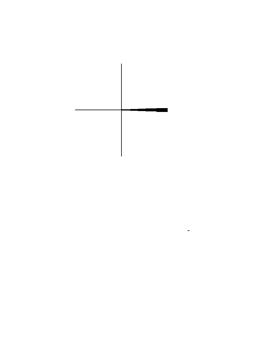
86
Cylindrical ends
............................
.
.
.
.
.
.
.
.
.
.
.
.
.
.
.
.
.
.
.
.
.
.
.
.
.
.
.
.
.
.
.
.
.
.
.
.
.
.
.
.
.
.
.
.
.
.
.
.
.
.
.
.....
......
......
......
......
......
......
......
......
......
......
......
......
......
......
......
......
......
......
...........
..........
......
..........
.
..........
.....
.
.
.
.
.
.
.
.
.
.
.
.
.
.
.
.
.
.
.
.
.
.
.
.
.
.
.
.
.
.
.
.
|
|
|
|
|
| = threshold
× = eigenvalue
× ×
×
Re σ
Im σ
Fig. 12. Spectrum of the Laplacian of an exact b-metric
Proposition 7.1
12
For a product-type metric
N
pp
(λ) ≤ C(1 + |λ|)
dim X
.
(7.10)
The behaviour of the continuous spectrum and the related definition
of the scattering matrix can be obtained, as in the case of Euclidean
scattering, by analytic continuation of the resolvent.
Theorem 7.1
13
The resolvent (∆ −λ
2
)
−1
extends, as an operator from
˙
C
∞
(X;
b
Λ
k
) to C
−∞
(X;
b
Λ
k
), to a meromorphic function of λ ∈ D where
D is the minimal Riemman surface to which all the functions (λ
2
−τ
j
2
)
1
2
extend to be holomorphic, as τ
j
2
runs over the set of thresholds.
12
The first result of this general type is due to Donnelly, [18], who showed that
N
pp
(λ) ≤ C(1 + |λ|)
2 dim X−1
.
(7.9)
The improvement of this estimate to (7.10) is due to Christiansen and Zworski,
[16], their proof uses a form of the ‘pseudo-Laplacian’ of Lax-Phillips and Colin
de Verdi`
ere, which in turn is very closely related to the Atiyah-Patodi-Singer
boundary condition discussed below.
13
In fact one can be much more precise about the structure of the Schwartz kernel
of the analytic continuation of the resolvent, see [73].

7.3 Scattering matrix
87
7.3 Scattering matrix
From the limiting absorption principle, i.e. an examination of the limit
of the resolvent as the parameter approaches the spectrum, a paramet-
rization of the generalized eigenspaces can be obtained much as in the
Euclidean case.
Proposition 7.2
If τ
j
2
is an eigenvalue of the boundary Laplacian and
φ is an associated eigenfunction, ∆
∂
φ = τ
j
2
φ, then for each λ ∈ R
with λ
2
> τ
j
2
such that λ
2
is not a threshold
14
there exists a unique
eigenfunction, with eigenvalue λ
2
, of the Laplacian satisfying
15
u = x
i
√
λ
2
−τ
j
2
φ +
X
τ
k
2
<λ
2
x
−i
√
λ
2
−τ
j
2
ψ
k
+ u
′
, u
′
∈ L
2
b
(X)
(7.11)
and u ⊥ v ∀ v ∈ L
2
b
(X) with (∆ − λ
2
)v = 0.
(7.12)
The sum in (7.11) is over the thresholds smaller than λ
2
and the
coefficients, ψ
k
, are associated eigenfunctions. Let
Eig(λ) =
X
τ
k
<λ
2
null(∆
∂
− τ
k
2
)
(7.13)
be the direct sum of the eigenfunctions for the boundary Laplacian with
eigenvalue less than λ
2
. The coefficient ψ
k
in (7.11) are determined by
φ so the map
φ 7−→
M
k
(
√
λ
2
− τ
k
2
p
λ
2
− τ
j
2
ψ
k
) ∈ Eig(λ)
(7.14)
extends by linearity to a map
A(λ) : Eig(λ) −→ Eig(λ).
(7.15)
This is the scattering matrix,
16
at frequency λ, for the metric. The λ-
dependent factors are included to make the scattering matrix unitary.
Note that it is a matrix, at least in the sense of an operator on a finite
dimensional space, with the caveat that the dimension of the space in-
creases every time λ
2
crosses a threshold, the change being the dimension
of the associated eigenspace of the boundary Laplacian.
17
14
i.e. is not an eigenvalue of the boundary Laplacian.
15
Here L
2
b
(X) is the L
2
space for any b-metric on X; the volume form is
dx
x
dy
near the boundary. Since the generalized eigenfunction in (7.11) is bounded and
L
2
eigenfunctions decay, as stated in Footnote 11, the pairing condition in (7.12)
does make sense.
16
As normalized by Christiansen in [15]; the normalization in [73] is different.
17
The results here are stated for the Laplacain on functions. For the Laplacian
on forms essentially the same result holds, except that the ‘boundary Laplacian’

88
Cylindrical ends
7.4 Boundary expansions and pairing
To see the unitarity of A(λ), and other things besides, it is convenient
to consider a limiting form of Green’s theorem in this setting. For any
λ ∈ R suppose u ∈ C
−∞
(X;
b
Λ
k
)
18
and that u satisfies (∆ − λ
2
)u ∈
˙
C
∞
(X;
b
Λ
k
). Then, for product-type metrics, and for λ
2
not a threshold,
u necessarily has a complete asymptotic expansion at the boundary in
the sense that
u ∼
X
j
x
µ
±
(j)
φ
j,±
, µ
±
(j)
2
= τ
j
2
− λ
2
,
(7.17)
where φ
j,±
are eigenfunctions, with eigenvalue τ
j
, for the boundary Lap-
lacian. Notice that the assumption that the solutions are of polynomial
growth means that there can only be a finite number of terms with neg-
ative powers of x.
19
If λ
2
= τ
j
2
for some threshold then there is just
one corresponding µ(j) = 0 and in place of (7.17) one must allow the
possibility of a logarithmic term:
u = φ
j,0
+ log x · φ
j,1
+
X
p6=j
x
µ
±
(p)
φ
p,±
,
µ
±
(p)
2
= τ
p
2
− τ
j
2
, λ
2
= τ
j
2
.
(7.18)
Here the φ
p,±
are eigenfunctions as before
20
and φ
j,i
are eigenfunctions
for the boundary Laplacian with eigenvalue τ
j
2
.
21
should be interpreted as the matrix of operators arising from (7.7), i.e.
∆
∂,k−1
0
0
∆
∂,k
.
(7.16)
18
This just means that u can be written as (a finite sum of sections of the form bundle
of the type) x
−N
B
N
v where v is square-integrable and B
N
∈ Diff
N
b
(X;
b
Λ
k
) for
some N. Thus u is of at worst ‘polynomial growth’ near the boundary.
19
Hence there can only be a finite number of terms with power having real part less
than any given real number p. It follows that the asymptotic expansion makes
sense.
20
See Footnote 17.
21
For a general exact b-metric something very similar is true. There is an asymptotic
expansion (7.17), or (7.18), as λ
2
is not, or is, a threshold, but the coefficients φ
j,±
cannot be taken to be constant. In fact they may not even be smooth but are
necessarily of the form
φ
j,±
∼
∞
X
r=0
x
N (r,j)
(log x)
r
φ
j,±,r
.
(7.19)
Here the coefficients φ
j,±,r
are all smooth and N (r, j) → ∞ as r → ∞ for each
j, so the sum makes sense asymptotically. The leading parts φ
j,±,0 ¯
(x = 0) are
eigenfunctions as before. The logarithmic terms in (7.19) arise only because of

7.5 Hodge theory
89
The boundary pairing is mostly of interest for ‘extended L
2
solutions.’
Thus, consider the space which is just a little larger
22
than L
2
x
0−
L
2
b
(X;
b
Λ
k
) =
\
ǫ>0
x
−ǫ
L
2
b
(X;
b
Λ
k
).
(7.20)
Proposition 7.3
If λ
2
is not a threshold and u
(i)
∈ x
0−
L
2
b
(X;
b
Λ
k
) for
i = 1, 2 satisfy (∆ − λ
2
)u
(i)
∈ ˙C
∞
(X;
b
Λ
k
) then
23
Z
X
h(∆ − λ
2
)u
(1)
, u
(2)
i − hu
(1)
, (∆ − λ
2
)u
(2)
i
dg
=
X
τ
j
2
<λ
2
2i
q
λ
2
− τ
j
2
Z
∂X
hφ
(1)
j,+
, φ
(2)
j,+
i − hφ
(1)
j,−
, φ
(2)
j,−
i
dh.
(7.21)
If λ
2
= τ
k
2
is a threshold then the right side of (7.21) is replaced by
2i
Z
∂X
hφ
(1)
k,1
, φ
(2)
k,0
i−hφ
(1)
k,0
, φ
(2)
k,1
i
dh
+
X
τ
j
2
<τ
k
2
2i
q
τ
k
2
− τ
j
2
Z
∂X
hφ
(1)
j,+
, φ
(2)
j,+
i − hφ
(1)
j,−
φ
(2)
j,−
i
dh.
(7.22)
7.5 Hodge theory
It turns out that the Hodge cohomology
24
of an exact b-metric is the
same as that of a scattering metric:
Proposition 7.4
The null space of the Laplacian, acting on square-
-integrable k-forms, is naturally isomorphic to the image of the relative
(deRham) cohomology of X in the absolute cohomology.
In fact quite a lot more can be said about ‘nearly square-integrable’
solutions.
25
Consider the ‘extended L
2
null space.’ As a special case
accidental multiplicities, when two of the µ
±
(j) differ by an integer. In case λ
2
is
a threshold a similar modification is needed to (7.18).
22
Here L
2
b
is just the metric L
2
space, in fact independent of choice of b-metric.
23
Here I have only written the formulæ in the case of a product-type metric. In the
general case the result is the same, except for instance that the terms on the right
in (7.21) are the leading coefficients in (7.19).
24
The modifications required in the discussion above when the boundary of X has
more than one component are rather minor. The boundary operator should just
be interpreted as the direct sum of the operators on the different components and
sums, as in (7.21) are over the eigenvalues of all these operators.
25
See Chapter 5 of [73] for a more detailed discussion.

90
Cylindrical ends
of (7.18) or (7.19), if u ∈ x
0−
L
2
b
(X;
b
Λ
k
) is in the null space of the
Laplacian then near the boundary it takes the form
u = (u
10
+ u
11
log x) ∧
dx
x
+ (u
00
+ u
01
log x) + u
′
, u
′
∈ L
2
b
(X;
b
Λ
k
)
(7.23)
where the u
ij
are k − i forms on ∂X, independent of x, which are in the
null space of the boundary Laplacian, i.e. they are harmonic.
The range of this generalized boundary data, given by the u
ij
’s, is a
Lagrangian subspace of the symplectic vector space formed by the direct
sum of two copies of the Hodge cohomology of ∂X in dimensions k − 1
and k. Moreover, both the relative and the absolute cohomology of X
can be ‘found’ in this extended L
2
null space:
Theorem 7.2
The relative cohomology of X is naturally identified with
the space of harmonic forms in x
0−
L
2
b
(X;
b
Λ
k
) such that u
00
= 0, u
01
= 0
and u
11
= 0 in (7.23), and similarly the absolute cohomology is naturally
identified with the space of harmonic forms in x
0−
L
2
b
(X;
b
Λ
k
) such that
u
00
= 0, u
10
= 0 and u
11
= 0. All these forms are closed and coclosed.
7.6 Atiyah-Patodi-Singer index theorem
A b-differential operator P ∈ Diff
m
b
(X; E, F ), acting from sections of
one vector bundle E to those of another bundle, F, has an invariantly
defined principal symbol,
σ
b,m
(P ) ∈ C
∞
(
b
T
∗
X; π
∗
hom(E, F )).
(7.24)
Here π :
b
T
∗
X −→ X is the projection and σ
b,m
(P ) is a homogeneous
polynomial of degree m on the fibres of
b
T
∗
X. As in the last lecture I
prefer to replace
b
T
∗
X by its stereographic compactification
b
¯
T
∗
X.
26
The new part added to compactify the vector bundle is just
b
S
∗
X, the
sphere bundle of
b
T
∗
X. Then the symbol map (7.24) can be regarded
as a map
σ
b,m
(P ) ∈ C
∞
(
b
S
∗
X; π
∗
hom(E, F ) ⊗ Q
m
).
(7.25)
where Q
m
is the bundle over
b
S
∗
X whose sections are the functions
which are homogeneous of degree m on
b
T
∗
X. The differential operator
26
This is a compact manifold with corner, it is actually diffeomorphic to
sc
¯
T
∗
X, just
not naturally so.

7.6 Atiyah-Patodi-Singer index theorem
91
is elliptic,
27
as an element of Diff
m
b
(X; E, F ) if σ
b,m
(P )(ζ) is, for each
ζ ∈
b
T
∗
X \ 0, invertible as a map from E
π(ζ)
to F
π(ζ)
. The symbol of P
in (7.5) is just
σ
b,m
(P ) =
X
k+|α|=m
p
k,α
(x, y)λ
k
η
α
.
(7.26)
As well as this symbol there is a closely related ‘non-commutative bound-
ary symbol.’ In fact this ‘indicial operator’ operator,
I(P, λ) =
X
k+|α|≤m
p
k,α
(0, y)λ
k
D
α
y
,
(7.27)
is an element of Diff
m
(∂X; E
∂X
, F
∂X
) which depends polynomially on
λ ∈ C . It is invariantly defined, except that it depends mildly on the
choice of boundary defining function, x.
The b-Sobolev spaces, of positive integral order, are defined quite
analogously to the usual ones:
H
k
b
(X; E) =
n
u ∈ L
2
b
(X; E); Diff
k
b
(X; E)u ⊂ L
2
b
(X; E)
o
.
(7.28)
Theorem 7.3
28
An element P ∈ Diff
m
b
(X; E, F ), where X is a compact
manifold with boundary, is Fredholm as an operator P : H
m
b
(X; E) −→
L
2
b
(X; F ) if and only if it is elliptic and has indicial operator I(P, λ) :
C
∞
(∂X; E
∂X
) −→ C
∞
(∂X; F
∂X
) invertible for each real λ.
If X is a spin manifold
29
the spin bundle, S, over X is defined and
the Dirac operator associated to an exact b-metric is an elliptic element
of Diff
1
b
(X; S). If X is even-dimensional then S = S
+
⊕ S
−
splits as a
direct sum of two subbundles and ð is ‘Z
2
-graded odd’ i.e. decomposes
as an anti-diagonal 2 × 2 matrix
ð
=
0
ð
−
ð
+
0
.
(7.29)
Over the boundary, S
+
and S
−
can be identified in a natural way and
in terms of this identification the indicial family of ð
+
is just the family
ð
0
+ iλ, where ð
0
is the (self-adjoint) Dirac operator on the boundary
27
One should perhaps say ‘b-elliptic’ to distinguish this condition from ellipticity in
the ordinary sense, since this it is impossible for P to be elliptic in this stronger
sense if m > 0 (and the two ellipticities are the same for m = 0) there should be
no confusion, with the meaning is clear from the context.
28
This is a generalization of traditional results for ordinary differential operators
with regular-singular points. It was proved in this generality in [75].
29
For a discussion of these matters, and the Atiyah-Patodi-Singer theorem itself, see
[73].

92
Cylindrical ends
defined by the induced spin structure. The indicial family is therefore
invertible for all real λ if and only if it is invertible for λ = 0, i.e. when
ð
0
itself is invertible. Thus Theorem 7.3 shows that ð
+
: H
1
b
(X; S
+
) −→
L
2
b
(X; S
−
) is Fredholm if and only if ð
0
is invertible.
Theorem 7.4
30
If X is an even-dimensional compact spin manifold
with boundary then ð
+
, the positive Dirac operator, is Fredholm if and
only if the boundary Dirac operator ð
0
is invertible, its index is then
31
ind(ð
+
) = dim null(ð
+
) − dim null(ð
−
) =
Z
X
b
A −
1
2
η(ð
0
)
where η(ð
0
) =
1
√
π
∞
Z
0
t
−
1
2
Tr ð
0
exp(−tð
2
0
)
dt.
(7.30)
7.7 b-Pseudodifferential operators
As in Section 6.5 the possibility of extending the Atiyah-Patodi-Singer
index theorem to a general index theorem for b-differential, or even
b-pseudodifferential operators is of considerable interest. As far as I
know this has not been done in a completely satisfactory way.
32
The
algebra of pseudodifferential operators, Ψ
∗
b
(X; E), which ‘microlocalizes’
the algebra Diff
∗
b
(X; E) is relatively straightforward to define. I shall
simply remark on some of its properties; see [68], [44] (Section 18.3) or
[73] for the definition.
33
Other closely related classes of operators have
been defined by Kondratev[50], Plamenevskii [93] and Schulze [102].
34
For any m ∈ R and any vector bundle E over X, Ψ
∞
b
(X; E) consists
of a linear space of operators on C
∞
(X; E) which is filtered by the order
30
This is the Atiyah-Patodi-Singer index theorem for the Dirac operator for a spin
structure. It has rather direct extensions to more general Dirac operators as-
sociated to Hermitian Clifford modules, as discussed, for example, in [73]. For
more general ‘family index theorems’ of Atiyah-Patodi-Singer type see the work
of Bismut and Cheeger [10], [77], [78].
31
The
b
A-genus here is the characteristic class, expressed in terms of the Riemann
curvature by
b
A = det
1
2
R/4πi
sinh(R/4πi)
. The convergence of the integral defining
the η invariant of the boundary Dirac operator also requires justification.
32
However, see the work of Piazza [92] for a partial result.
33
See [76] for a brief discussion in the case of manifolds with corners.
34
There is a difference between the calculus Ψ
∗
b
(X; E) and the others listed here
arising from the different intended applications, to complete manifolds on the
one hand and incomplete manifolds with conical singularities on the other. For
a general discussion of pseudodifferential operators on complete manifolds with
bounded geometry see the lectures of Shubin [107].

7.8 Trace formula and spectral asymptotics
93
m and
Diff
m
b
(X; E) ⊂ Ψ
m
b
(X; E) ∀ m ∈ N.
(7.31)
The symbol map is defined, consistently with (7.26) and this inclusion,
as a map onto the space C
∞
(
b
S
∗
X; π
∗
hom(E) ⊗ Q
m
) of sections which
are homogeneous of degree m. This symbol map is multiplicative and
gives a short exact sequence
σ
b,m+m
′
(P Q) = σ
b,m
(P ) · σ
b,m
′
(Q),
(7.32)
0 −→ Ψ
m−1
b
(X; E) −→ Ψ
m
b
(X; E)
σ
b
,m
−→ C
∞
(
b
S
∗
; π
∗
hom(E) ⊗ Q
m
) −→ 0.
(7.33)
Furthermore the map to the indicial family, (7.27), also extends to the
algebra of b-pseudodifferential operators, it takes values in the space of
entire functions with values in Ψ
m
(∂X; E
∂X
) with appropriate unifor-
mity properties in the complex parameter λ. Furthermore Theorem 7.3
extends to the pseudodifferential operators essentially verbatim to char-
acterize the Fredholm elements of the algebra.
7.8 Trace formula and spectral asymptotics
As already noted above the trace formula has been extended, by Chris-
tiansen, to exact b-metrics. If x ∈ C
∞
(X) is a boundary defining func-
tion with respect to which the metric takes the form (7.1) and U
g
(t) is
the wave group as in (4.2), but on X, then the b-trace can be defined,
as a tempered distribution, by Hadamard regularization:
τ
g
(ρ) = b-Tr U (ρ) = lim
ǫ↓0
Z
x>ǫ
tr
Z
R
U (t, p, p)ρ(t)dt dg(p) − A(ρ) log ǫ
,
(7.34)
where tr is just the trace on 2 × 2 matrices and A(ρ) is determined by
the condition that the limit exist.

94
Cylindrical ends
Proposition 7.5
35
For any exact b-metric the inverse Fourier trans-
form of the b-trace (7.34) of the wave group satisfies
F
−1
τ
g
=
X
(λ
′
)
2
∈ppspec(∆)
δ(λ − λ
′
) +
1
2πi
d
dλ
log det A(λ)
+
1
4
X
06=σ
2
∈spec(∆
0
)
δ(λ − σ) +
1
2
Tr A(0)δ(λ).
(7.35)
Using this trace formula Christiansen and Zworski have shown that the
sum of the counting function for the point spectrum and the scattering
phase has a leading ‘Weyl’ term as λ → ∞ :
N
pp
(λ) +
1
2πi
log det A(λ) = (2π)
−n
Vol(B
n
)b- Vol(X)λ
n
+ O(λ
n−1
)
where b- Vol(X) =
bZ
X
dg = lim
ǫ↓0
Z
x>ǫ
dg + log ǫ Vol(∂X)
(7.36)
is the regularized ‘b-volume’ of the manifold.
7.9 Manifolds with corners
There are many interesting possible extensions of these results. In par-
ticular it is natural to seek similar descriptions of the index, spectral and
scattering theory for similar exact b-metrics on manifolds with corners.
These are easily defined inductively. Indeed a compact manifold with
corners, X, has a product decomposition in a neighbourhood of each of
its boundary hypersurfaces of the form [0, ǫ) × H where the boundary
hypersurface, H, is a compact manifold with corners where the maxi-
mum codimension of a boundary face is at most one less than in X. Thus
if, for each boundary hypersurface H, x
H
is a defining function for H
then an exact b-metric of product type on X is a metric on the interior
which takes the form
g = (
dx
H
x
H
)
2
+ g
′
H
near H
(7.37)
35
The scattering phase, log det A(λ) has to be normalized at each threshold, since
the rank of A(λ) changes there. The normalization of the jump of the phase used
here, following [15], involves the behaviour of the generalized eigenfunctions. This
is important since it contributes δ terms to the formula.

7.9 Manifolds with corners
95
where g
′
H
is an exact b-metric of product type on H. It is rather clear
that one should expect.
36
Conjecture 7.1
For an exact b-metric
37
the spectrum of the Laplacian
consists of possibly countable point spectrum of finite multiplicity, cor-
responding to L
2
eigenfunctions together with continuous spectrum con-
sisting of an at most countable union of rays [τ, ∞) where the thresholds,
τ, form the discrete set consisting of the union of the L
2
eigenvalues for
the induced Laplacians on all boundary faces (of positive codimension.)
38
Notice that Euclidean spaces are themselves examples of these types
of manifolds. So are products of manifolds with corners, carrying exact
b-metrics. In both these cases this conjecture is easily verified.
It would also be interesting to extend the Atiyah-Patodi-Singer index
theorem to Dirac operators on such manifolds. At this stage there seems
to be no general result except under the (unreasonable) assumption
that the induced Dirac operator on every boundary face of codimension
greater than 1 is invertible. Then a result very similar to Theorem 7.4
holds.
39
36
I hope to prove this soon!
37
Whether of product type or not.
38
In fact one should expect to be able to show that the ray of continuous spectrum
arising from an L
2
eigenvalue on a boundary face of codimension p corresponds
to functions on a (pseudo-) manifold of dimension p − 1. Part of the problem is to
know exactly what is meant by a pseudomanifold here!
39
Partial results on the behaviour of the eta invariant for the boundary of a manifold
with corners up to codimension two are contained in [60] and [35].

8
Hyperbolic metrics
In the previous two lectures I discussed two classes of complete metrics
on the interiors of compact manifolds with boundaries. Today I will
discuss two more,
1
necessarily in less detail. To start with let me briefly
consider the classification of metrics which are ‘warped products’ near
the boundary.
8.1 Warped products
Thus, if X is a manifold with boundary and x is a boundary defining
function consider a metric which takes the form
g = x
2a
dx
2
+ x
2b
h
(8.1)
where at least initially it can be supposed that h is a metric on the
boundary pulled back under some product decomposition, i.e. is inde-
pendent of x and has no dx terms. Such a metric is complete
2
if and
only if
a ≤ −1.
(8.3)
1
In a sense three more.
2
A metric is complete if and only if every geodesic can be continued indefinitely in
both directions. If X is compact then the only failure of completeness that can
occur must involve a geodesic which approaches the boundary. Certainly condition
(8.3) is necessary since the curves which are constant in the boundary factor are
geodesics and these have infinite arclength in the direction in which x is decreasing
if and only if
1
Z
0
x
−a
dx = ∞
(8.2)
which is just (8.3). The converse involves a closer look at the geodesic equations
but is not very difficult.
96

8.1 Warped products
97
I shall call the case a = −1 ‘marginally complete.’
3
In the marginally complete case the sign of b is the determining fea-
ture. Indeed, for any constant q > 0 the transformation x
′
= x
q
, whilst
not smooth, is continuous and the introduction of x
q
as a boundary defin-
ing function simply changes the C
∞
structure on X near the boundary.
Thus in these cases, and even if h involves both dx and x dependence of
the coefficients, the distinguished cases
4
are
5
g =
dx
2
x
2
+ x
2
h,
‘hc’=hyperbolic, or rank one, cusp
(8.4)
g =
dx
2
x
2
+ h,
‘b’=boundary or metric with cylindrical end
(8.5)
g =
dx
2
x
2
+
h
x
2
,
‘0’=zero or conformally compact metric.
(8.6)
The first and last of these are the cases I wish to discuss today. The
middle one is of course the subject of Lecture 7.
Now consider the ‘overcomplete’ cases, where a < −1. There is a basic
classification corresponding to the sign of b − a − 1. If this vanishes then
the, possibly singular, transformation x 7−→ x
′
= x
−1/(1+a)
reduces the
metric to a constant multiple of the scattering metric
g
sc
= x
−2
dx
2
x
2
+ h
=
dx
2
x
4
+
h
x
2
,
‘sc’=scattering,
(8.7)
considered in Lecture 6. If b < 1 + a (which is, by assumption, negative)
then the transformation x
′
= x
−b/(1+a)
reduces the metric to a constant
multiple of the singular conformal 0-metric
g = x
−2r
dx
2
x
2
+
h
x
2
,
r =
(1 + a)
2
b
> 0.
(8.8)
In the remaining cases, where b > 1 + a, the metric is conformal, with
a possibly singular conformal factor, to the ‘hyperbolic cusp’ type metric
in (8.4). It is worth noting the three subcases. First if (1 + a) < b < 0
3
One should be a little careful about ‘degrees of completeness’ since this is rather
subjective. See Footnote 6.
4
There does not seem to be any uniformity in the names or notation for these
various types of metrics. I like to have abbreviations, such as ‘0-’ in order to be
able to denote in a simple way the various objects that are ‘functorially’ associated
to these types of metrics, e.g. the ‘0-pseudodifferential operators’ discussed below.
A rather more complete discussion of how one can associate such objects with
these classes of metrics (and many others, a couple more of which are mentioned
below), is to be contained in [66]. Maybe it exists by now?
5
Here and below I consistently switch to the old notation, x, for the new boundary
defining function.

98
Hyperbolic metrics
then the metric can be transformed to a constant multiple of
g = x
−2r
dx
2
x
2
+ x
2
h
with r > 1.
(8.9)
In case b = 0 again a, possibly singular, transformation x 7−→ x
′
=
x
−1−a
can be made reducing the metric to a constant multiple of the
case
6
g
c
=
dx
2
x
4
+ h
‘c’=cusp.
(8.10)
In the remaining case of b > 0 a similar transformation leads to the
remaining case intermediate between (8.4) and (8.10)
g = x
−2r
dx
2
x
2
+ x
2
h
with 0 < r < 1.
(8.11)
In summary then there are eight basic cases. I do not know of any
serious examination of (8.8), (8.9) or (8.11). The other cases have all
been treated to a greater or lesser extent. A similar classification can be
made in the incomplete cases.
8.2 Conformally compact manifolds
The first case I shall discuss is a metric of the form (8.6) near the bound-
ary. For the most part the assumption that h is independent of x and
dx can be dropped, this only affects the more subtle results.
The basic example of such a metric is that on hyperbolic space. In
the upper-half space model, n-dimensional
7
hyperbolic space is just
8
H
n
=
(x, y) ∈ R
n
; x > 0, y ∈ R
n−1
(8.12)
with the metric
g =
|dx|
2
+ |dy|
2
x
2
.
(8.13)
Clearly this is of the form (8.6) down to x = 0. Of course this is not a
6
Notice that the transcendental transformation x 7−→ x
′
= 1/ log(1/x) reduces
the cusp metric in (8.10) to the metric (8.5). Of course if one has a variable
coefficient form of (8.10), where h depends on x then this introduces rather singular
coefficients in (8.5), so one should really think of smooth perturbations of (8.5) as
a special case of smooth perturbations of (8.10).
7
n ≥ 2.
8
In most discussions of hyperbolic space the role of the variables in (8.12) is reversed,
i.e. the boundary defining functions is denoted y and the x’s are variables in R
n−1
.
I think it is better to keep to the consistent usage of x as a boundary defining
function.

8.2 Conformally compact manifolds
99
compact manifold with boundary but it can be compactified to a Eu-
clidean ball so that the hyperbolic metric is a 0-metric. I shall denote
the compact model by ¯
H
n
.
There are other examples of 0-metrics which arise from hyperbolic
space. The group of diffeomorphism of H
n
preserving the metric is
PSL(n, R), acting as fractional linear transformations. Consider Γ which
is a subgroup acting discretely.
9
If Γ has no fixed points (in the interior)
then H
n
/Γ is a manifold, although it can be rather nasty. If the group Γ
is ‘small’ in the sense that it has no parabolic elements and is geometri-
cally finite
10
then the quotient
11
¯
H
n
/Γ is again a compact manifold with
boundary to which the hyperbolic metric descends as a 0-metric. The
extension of scattering theory to hyperbolic space, and its quotients, has
quite a long history; in particular Lax and Phillips extended their theory
to this setting, see especially [54] and references therein.
The metric on hyperbolic space is very special in that its sectional
curvature is a negative constant. A general 0-metric is not so restricted.
Let me write (8.6) in the form
g =
g
∞
x
2
(8.14)
where g
∞
is an incomplete metric which is smooth up to the boundary,
i.e. is just a smooth positive definite metric on the fibres of T X.
12
Even
so such a 0-metric has ‘asymptotically constant curvature’ in the weak
sense that if p ∈ ∂X and p
n
∈ X
◦
is a sequence with limit p then the
sectional curvatures at p
n
approach the fixed value −|dx|
2
∞
, where |·|
∞
is
the dual metric on T
∗
X to the metric g
∞
. This suggests a strengthening
of (8.14) by adding the condition
|dx|
∞
= 1 on ∂X.
(8.15)
This implies that, for an appropriate choice of product structure,
g =
dx
2
+ h(x)
x
2
near ∂X,
(8.16)
where h is a metric on the cross-section of the product, i.e. on ∂X
but depending parametrically on x. This can be further restricted by
9
Meaning that for any compact subset, K, of the interior of H
n
the set of γ ∈ Γ
such that γ(K) ∩ K 6= ∅ is finite.
10
For a full discussion of this condition see the paper of Bowditch [11].
11
Examples are given by the Schottky groups.
12
Alternatively this is the same as demanding that g
∞
be the restriction to X of a
Riemann metric on 2X, its double to a compact manifold without boundary.

100
Hyperbolic metrics
demanding that h(x) be independent of x :
g =
dx
2
+ h
x
2
near ∂X.
(8.17)
Any compact manifold with boundary has a metric of this form.
8.3
0-geometry and analysis
By 0-geometry I mean the geometry of a conformally compact metric,
(8.14), or more generally the geometry of the more fundamental object,
V
0
(X), which is the space of smooth vector fields on X of bounded length
with respect such a metric. These structures were first discussed in this
degree of generality by Mazzeo [59] and then in [61]. The space V
0
(X)
is independent of the particular 0-metric chosen
V
0
(X) = {V ∈ V(X); |V |
∞
≤ Cx} = xV(X) ⊂ V
b
(X).
(8.18)
It consists of the vector fields which vanish
13
at the boundary. Again it is
a Lie algebra. It has certain other properties
14
which mean that one can
follow through much of the abstract discussion of differential operators
on compact manifolds without boundary. Thus, as in the cases of the
sc and b-structures, the filtration of the enveloping algebra of V
0
(X),
Diff
m
0
(X), is defined, as consisting of those operators
P : C
∞
(X) −→ C
∞
(X)
(8.19)
which can be written as a sum of up to m fold products of vector fields
in V
0
(X).
15
This definition can be extended, by localization, to define
the filtered algebra Diff
∗
0
(X; E) of operators on sections of any vector
bundle over X.
There is also a natural 0-tangent bundle,
0
T X. This can be defined
either by ‘rescaling,’ so it can be denoted xT X or, as in Footnote 7.4,
more abstractly so that
V
0
(X) = C
∞
(X;
0
T X).
(8.20)
Its dual bundle,
0
T
∗
X, plays the rˆ
ole of T
∗
X for these operators. In par-
ticular the standard symbol map extends by continuity from the interior
to a map
σ
0,m
: Diff
m
0
(X; E) −→ C
∞
(
0
S
∗
X; π
∗
hom(E) ⊗ Q
m
),
(8.21)
13
Hence the ‘0’ moniker.
14
I collect such properties together in the notion of a ‘boundary fibration structure’
discussed in [66].
15
The fact that V
0
is a Lie algebra makes the order well defined.
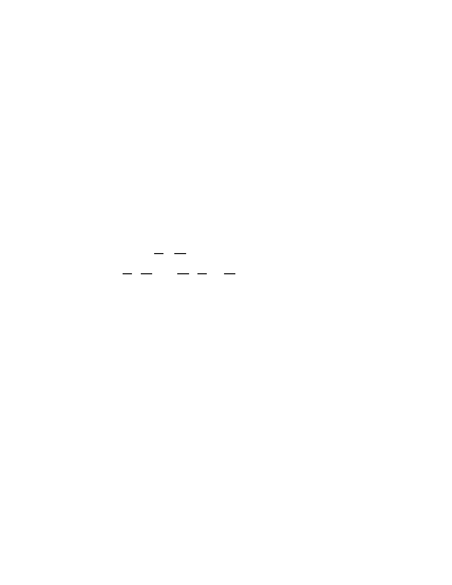
8.3 0-geometry and analysis
101
where
0
S
∗
X is the sphere bundle over X with fibre at each point the
sphere at infinity
16
and Q
m
is the restriction to
0
S
∗
X of the line bundle
with sections the functions on
0
T
∗
X which are homogeneous of degree
m on the fibres. The null space of (8.21) is precisely Diff
m−1
0
(X; E).
As in the other cases of such rings of differential operators discussed
above, this symbol map does not fix the important properties
17
of such
operators. The second ‘symbol’ map is, as in the b-case, non-commut-
ative. In fact it is ‘partly commutative’ and partly non-commutative.
To describe it precisely observe that, for each p ∈ ∂X,
0
T
p
X has a non-
trivial Lie algebra structure. Namely if v, w ∈
0
T
p
X and V, W ∈ V
0
(X)
are such that V (p) = v and W (p) = w
18
then
[v, w] = [V, W ](p) ∈
0
T
p
X
(8.22)
is independent of the choice of V and W.
19
This makes
0
T
p
X into a
solvable Lie algebra
20
which is given in terms of the basis
x
∂
∂x
, x
∂
∂y
j
, j = 1, . . . , n − 1, by
[x
∂
∂x
, x
∂
∂y
j
] = −[x
∂
∂y
j
, x
∂
∂x
] = x
∂
∂y
j
, j = 1, . . . , n − 1
(8.24)
with all other commutators zero. Let Diff
m
0,p
(
0
T
p
X) be the part of or-
der m of the enveloping algebra of this Lie algebra.
21
It is a finite-
dimensional vector space and these spaces form a bundle of algebras
over the boundary; I shall denote by Diff
m
I,0
(∂X) the smooth sections of
this bundle. The normal map is a surjective linear map
N : Diff
m
0
(X) −→ Diff
m
I,0
(∂X)
(8.25)
16
This is just the boundary of the stereographic compactification of
0
T
∗
p
X.
17
For instance the Fredholm condition.
18
In the sense of sections of
0
T X.
19
This independence of choice is just the fact that if I(p) ⊂ C
∞
(X) is the ideal of
functions vanishing at p ∈ ∂X then V
0
(X) · I(p) ⊂ I(p), so
[V
0
(X), I(p) · V
0
(X)] ⊂ I(p) · V
0
(X)
(8.23)
shows that I(p) · V
0
(X) ⊂ V
0
(X) is a Lie algebra ideal.
The quotient
V
0
(X)/ (I(p) · V
0
(X)) , which is, by definition, just
0
T
p
X, is therefore a Lie
algebra.
20
So the corresponding Lie group is diffeomorphic to the same space,
0
T
p
X, as the
Lie algebra and the group law can be written down quite explicitly.
21
If the Lie algebra
0
T
p
X is realized as the left-invariant vector fields on the corre-
sponding Lie group then Diff
m
0,p
(
0
T
p
X) consists of the operators on C
∞
functions
on the Lie group which are polynomials, with constant coefficients and degree at
most m, in these vector fields.

102
Hyperbolic metrics
which is a homomorphism of algebras.
22
I shall not go into any detail here, but part of the package of a
‘boundary fibration structure’ is that there is an associated ring of pseu-
dodifferential operators, in this case the 0-pseudodifferential operators
Ψ
∗,∗
0
(X; E), acting on sections of any given vector bundle, E. It has
properties closely related to those of Diff
∗
0
(X; E). The first of the orders
in Ψ
∗,∗
0
(X; E) is the interior order, as a pseudodifferential operator in
the ordinary sense, and the second order represents the degree of vanish-
ing, or singularity, at the boundary. If x is a boundary defining function
then
Ψ
m,l
0
(X; E) = x
l
Ψ
m,0
0
(X; E) ∀ m, l ∈ R.
(8.27)
Both the symbol map and the normal operator have natural extensions
to these spaces of pseudodifferential operators.
The Lie group with Lie algebra
0
T
p
X, p ∈ ∂X, has a natural com-
pactification, ¯
G
p
, to a half-ball on which the elements of the Lie algebra
are smooth vector fields. Acting on the natural 0-Sobolev spaces, as
they do, an element P ∈ Diff
m
0
(X; E), or Ψ
m,l
0
(X; E), is Fredholm if
and only if its symbol is an invertible homomorphism at each point and
its normal operator is invertible on the corresponding spaces on G
p
, for
each p ∈ ∂X. As far as I am aware, no general index theorem for this
algebra has been proved. However an index theorem of Plamenevskii
and Rozenblyum [94] can be regarded as a particular case of such a
conjectural result.
8.4 The Laplacian
One direct consequence of the 0-geometry just discussed is that the Lap-
lacian of a conformally compact metric, (8.14), is necessarily an element
of Diff
2
0
(X). In fact the same is true for the operator acting on forms,
provided these are rescaled. If
0
Λ
k
is the kth exterior power of
0
T
∗
X
then, for any k,
∆ ∈ Diff
2
0
(X;
0
Λ
k
).
(8.28)
The algebra of 0-pseudodifferential operators is designed so that
22
Thus
N (P · Q) = N (P ) · N (Q), P ∈ Diff
m
0
(X), Q ∈ Diff
m
′
0
(X).
(8.26)

8.4 The Laplacian
103
Proposition 8.1
For any conformally compact metric, with curvature
constant at infinity in the sense of (8.15), the (true) resolvent family
(∆ − τ )
−1
∈ Ψ
−2,0
0
(X), τ ∈ C \ [
(n − 1)
2
4
, ∞)
(8.29)
depends meromorphically on τ and the spectrum of ∆ consists of the
half-line [(n − 1)
2
/4, ∞) with possibly a finite number of eigenvalues, of
finite multiplicity, in (0, (n − 1)
2
/4).
There is a similar result for the action on k-forms.
23
Under the as-
sumption that |dx|
∞
is constant
24
on the boundary, as in (8.16), there
are no embedded eigenvalues
25
and the spectrum has uniform, infi-
nite, multiplicity. More precisely the generalized eigenspaces can be
parametrized much as in the Euclidean case.
Proposition 8.2
26
For a metric (8.16), each 0 6= λ ∈ R and each
f ∈ C
∞
(∂X) there is a unique solution of the equation (∆ − λ
2
−
1
4
(n −
1)
2
)u = 0 of the form
u = x
iλ
x
1
2
(n−1)
f + x
−iλ
x
1
2
(n−1)
f
−
+ u
′
, f
−
∈ C
∞
(∂X), u
′
∈ L
2
(X).
(8.31)
As usual the uniqueness of the solution in (8.30) leads to the scattering
matrix
A(λ) : C
∞
(∂X) −→ C
∞
(∂X).
(8.32)
In this case A(λ) ∈ Ψ
0
(∂X) is an invertible pseudodifferential operator,
on the compact manifold ∂X.
27
Even in the case of hyperbolic space
itself the scattering matrix is not ‘trivial.’
The key to understanding the behaviour of the scattering matrix, in
particular why it is a pseudodifferential operator, lies in the behaviour
23
See the paper of Mazzeo [58].
24
These results can be extended to the case of a ‘variable curvature at infinity’ to
some degree, see [58].
25
See R. Mazzeo [59].
26
As in the case discussed above this can be refined to give a functional parametriz-
ation of the continuous spectrum. Namely for given f ∈ C
−∞
(∂X) there is still
a unique generalized eigenfunction of the form (8.31), where f
−
∈ C
−∞
(∂X) and
the error term u
′
is permitted to be in the Sobolev space
H
−∞,0
0
(X) = Diff
∗
0
(X) · L
2
(X), L
2
(X) = H
0,0
0
(X)
(8.30)
being the metric L
2
space. Furthermore these solutions exhaust the null space of
∆ − λ
2
−
1
4
(n − 1)
2
acting on C
−∞
(X) = H
∞,−∞
0
(X).
27
It is really of ‘complex order’ −2iλ.

104
Hyperbolic metrics
...........
..........
..........
...........
..........
..........
...........
...........
............
...........
............
..............
...............
................
...................
......................
...................................
......................................................................................
................
.............
............
..........
..........
.........
........
........
.......
........
.......
.......
.......
.......
......
......
......
......
......
......
......
......
......
......
......
......
.....
......
......
......
......
......
.
......
.....
....
....
...
...
...
..
...
..
..
..
..
..
..
..
..
.
..
..
.
..
.
..
.
..
.
..
.
..
.
.
.
..
.
.
.
..
.
.
.
.
..
.
.
.
.
.
.
.
.
.
.
.
.
.
.
.
.
.
.
.
.
.
.
.
.
.
.
.
.
.
.
.
.
.
.
.
.
.
.
.
.
.
.
.
.
.
.
.
.
.
.
.
.
.
.
.
.
.
.
.
.
.
.
.
.
.
.
.
.
.
.
.
.
.
.
.
.
.
.
.
.
.
.
.
.
.
.
.
.
.
.
.
.
.
.
.
.
.
.
.
.
.
.
.
.
.
.
.
.
.
.
.
.
.
.
.
.
.
.
.
.
.
.
.
.
.
.
.
.
.
.
.
.
.
.
.
.
.
.
.
.
.
.
.
.
.
.
.
.
.
.
.
.
.
.
.
.
.
.
.
.
.
.
.
.
.
.
.
.
.
.
.
.
.
.
.
.
.
.
.
.
.
.
.
.
.
.
.
.
.
.
.
.
.
.
.
.
.
.
.
.
.
.
.
.
.
.
.
.
.
.
.
.
.
.
.
.
.
.
.
.
.
.
.
.
.
.
.
.
.
.
.
.
.
.
.
.
.
.
.
.
.
.
.
.
.
.
.
.
.
.
.
.
.
.
.
.
.
.
.
.
.
.
.
.
.
.
.
.
.
.
.
.
.
.
.
.
.
.
.
.
.
.
.
.
.
.
.
.
.
.
.
.
.
.
.
.
.
.
.
.
.
.
.
.
.
.
.
.
.
.
.
.
.
.
.
.
.
.
.
.
.
.
.
.
.
.
.
.
.
.
.
.
.
.
.
.
.
.
.
.
.
.
.
.
.
.
.
...
.
.
.
.
.
.
.
...
.
.
.
..
.
.
..
.
.
..
.
.
..
.
...
..
.
..........
.
...........
.
..........
.
..........
.
..........
..........
.............
........
..........
...........
.............
...................
...................................................................................
....................
................
..............
.............
............
...........
...........
..........
...........
...........
...........
..........
..
...........
.
..
..........
.
..
..
..
..
.
..........
..
.
.
.
..
.
.
.
.
.
..
.
.
.
.
.
.
.
.
.
.
.
.
.
.
.
.
.
.
.
.
.
.
.
.
.
...............
...................................................................
.................
..............
...........
............
...........
...........
..........
..........
..........
..
..
.
...
.
...
.
.
.
.
...
.
.
.
.
.
.
.
.
.
.
.
.
.
.
.
.
.
.
.
.
.
.
.
.
.
.
.
.
.
.
.
.
.
.
.
.
.
.
.
.........................................................
..............
............
..........
..........
..........
..
..........
.
...
..
.
.
.
...
.
.
.
.
.
.
.
.
.
.
.
.
.
.
.
.
.
.
.
.
.
.
.
.
.
.
.
.
.
.
.
.
.
.
.
.
.
.....................
..........
..
..........
.
.
.
.
.
.
.
.
.
.
.
.
p
Fig. 13. Geodesics for a conformally compact metric
of the geodesics of the conformally compact metric. It is quite easy to
see that for every p ∈ ∂X there are many geodesics which have limit at p
as t → −∞. Moreover, given a neighbourhood of the boundary, {x < ǫ},
an infinite family of these geodesics stay within that neighbourhood and
have limit point, as t → ∞, also on the boundary. As ǫ ↓ 0 the end point
of such geodesics necessarily approaches p. Thus the boundary relation,
which for a scattering metric gives geodesic flow at length π for the
boundary metric, gives the identity relation for a conformally compact
metric.
I shall not discuss the Hodge cohomology of metrics of this type; this
has been worked out by Mazzeo [58]; see also the work of Mazzeo and
Phillips [63] where the cohomology of more general hyperbolic quotients
is computed.
8.5 Analytic continuation
The family of operators (∆−λ
2
−
1
4
(n−1)
2
)
−1
, where ∆ is the Laplacian
as in Proposition 8.1, extends to be a meromorphic function of λ ∈ C ,
as an operator from C
∞
c
(X
◦
)) to C
∞
(X
◦
). This was shown in [61], with
the caveat that the residues of the poles are not shown there to be of
finite rank. The finiteness of the rank in case the metric has constant
curvature near infinity is shown by Guillop´e and Zworski, in [32], [31].
They also show, under the same conditions, a polynomial bound on the

8.6 Finite volume quotients
105
counting function for the poles, defined as in (4.23),
N (R) ≤ C + CR
n+1
.
(8.33)
This is probably not optimal. For quotients of hyperbolic space of this
type the analytic continuation was also shown by Froese, Hislop and
Perry in [23]; see the references there for earlier work, especially that
related to hyperbolic quotients.
8.6 Finite volume quotients
The second class of metrics I wish to briefly discuss today are the hyper-
bolic cusp metrics, as in (8.4). One feature which immediately distin-
guishes these metrics from all the other complete metrics I have consid-
ered so far is that they have finite volume.
28
Indeed the most familiar
example of these sorts of metrics come from finite volume quotients of
hyperbolic space. Consider the quotient of hyperbolic space by the infi-
nite cyclic group generated by the single
29
transformation
x + iy 7−→ x + i(y + 1).
(8.34)
The quotient H
2
/Γ is a cylinder with metric (8.13), with |dy|
2
interpreted
as the metric on the circle. Notice in particular that this manifold with
boundary has two boundary hypersurfaces, one which is of type 0 and
the other of type ‘hc.’ The inversion x 7→ 1/x interchanges the two.
8.7 hc-geometry
The finiteness of the volume of manifolds with hc-metrics is not the
only novelty as compared to the other cases considered so far. In fact
the underlying difference is that the space of vector fields of bounded
length is not spanned by its smooth elements.
30
This is closely related
to the fact that the boundary
31
of a finite volume quotient is typically a
torus. Said a different way, the hc-structure is not a boundary fibration
28
The volume form near the boundary is necessarily of the form x
n−2
dxdy where dy
is a volume form on the boundary and n = dim X. Since n ≥ 2, for non-triviality,
this is integrable so the volume is finite.
29
This is a typical parabolic element of PSL(2, R)
30
It contains elements with unbounded coefficients of the type V /x with V a smooth
vector field tangent to the boundary but which does not vanish identically after
restriction to the boundary.
31
Meaning the boundary of the appropriate compactification of the quotient.

106
Hyperbolic metrics
structure in the sense of [66]. The simple remedy is to regard these
hc-metrics as conformal cusp metrics. That is, simply write (8.4) as
g
hc
= x
2
g
c
(8.35)
where g
c
is a metric of the form (8.10).
32
If Diff
∗
c
(X) is defined as the
enveloping algebra of the Lie algebra V
c
(X) of cusp vector fields
33
then
the Laplacian of an hc-metric is more singular
∆
hc
∈ x
−2
Diff
2
c
(X).
(8.36)
However, this means that the resolvent family can be written in the form
(∆
hc
− τ )
−1
= x
−2
(x
2
∆ − x
2
τ )
−2
∈ Ψ
−2,−2
c
(X).
(8.37)
Of course I have not defined the algebra, Ψ
m,k
c
(X), of cusp pseudodif-
ferential operators however I have already pointed out, in Footnote 6,
the relationship between the cusp- and b-algebras. Thus it is not too
hard to make sense of (8.37). What I really want to indicat here is that
it should lead one to expect, in general for an hc-metric, that the full
spectrum should behave like the spectrum of a b-Laplacian near 0. The
only real difference is that the spectrum will not in general start at 0.
8.8 Spectrum
The spectral theory of the Laplacian for metrics of this type has been
discussed in some detail by M¨
uller [83], following much work, by many
authors and over a long period of time, on the finite volume quotients
of hyperbolic space.
Proposition 8.3
The spectrum of the Laplacian of an hc-metric
34
con-
sists of continuous spectrum of finite multiplicity in [
1
4
(n − 1)
2
, ∞) with
the possibility of embedded L
2
(pure point) spectrum and also of a fi-
nite number of L
2
eigenvalues in [0,
1
4
(n − 1)
2
]. For each 0 6= λ ∈ R
32
This is one reason for singling out the ‘cusp’ metrics, but not the only one.
33
I have sloughed over some subtleties here. In distinction to the earlier cases, the
cusp structure is not ‘canonical.’ That is, the Lie algebra V
c
(X) is not invariant
under all diffeomorphisms of X. In fact it is equivalent to specifying a boundary
defining function up to quadratic terms or a constant multiple, i.e. it is equiva-
lent to a choice of trivialization of the conormal bundle to the boundary, up to
a constant factor. Under a general diffeomorphism of X one cusp structure is
transformed into another.
34
Of product type.

8.8 Spectrum
107
and each element, f, of the null space of ∆
∂
35
there is a solution of
(∆ −
1
4
(n − 1)
2
− λ
2
)u = 0 of the form
u = x
iλ
x
1−n
f + x
−iλ
x
1−n
f
−
+ u
′
, u
′
∈ L
2
hc
(X)
(8.38)
which is unique up to addition of an L
2
eigenfunction with eigenvalue
1
4
(n − 1)
2
+ λ
2
.
The scattering matrix in this case is a matrix! Namely it is a λ-
dependent linear operator on the finite-dimensional space consisting of
the null space of the boundary Laplacian. This is again easy to relate
to the behaviour of the geodesics. Indeed there is a neighbourhood of
the boundary which contains no complete geodesic. Again the resolvent
has a meromorphic continuation to the λ plane. For a discussion of the
poles of the continuation see the papers of Guillop´e and Zworski [32]
and Froese and Zworski [24]. The trace formula, giving the regularized
trace of the wave group in terms of the eigenvalues and the scattering
matrix is well-known in the case of hyperbolic quotients, as Selberg’s
trace formula, and extends to the general case in a similar form.
35
Note that the boundary may consist of several components. The null space of
∆
∂
on each component just consists of the constants, but these can differ from
component to component.

108
Hyperbolic metrics
References
[1] S. Agmon, Spectral theory of Schr¨
odinger operators on Euclidean
and non-Euclidean spaces, Comm. Pure Appl. Math. 39 (1986),
3–16.
[2] N. Anghel, L
2
-index formula for perturbed Dirac operators, Comm.
Math. Phys. 128 (1990), 77–97.
[3]
, On the index of Callias-type operators, Geom. and Funct.
Anal. 3 (1993), 431–438.
[4] M.F. Atiyah, K-theory, Benjamin, New York, 1967.
[5] M.F. Atiyah and I.M. Singer, The index of elliptic operators, III,
Ann. of Math. 87 (1968), 546–604.
[6] C. Bardos, J.-C. Guillot, and J. Ralston, La relation de Poisson
pour l’´equation des ondes dans un ouvert non born´e, Comm P.D.E.
7
(1982), 905–958.
[7] C. Bardos, G. Lebeau, and J. Rauch, Scattering frequencies and
Gevrey 3 singularities, Invent. Math. 90 (1987), 77–1144.
[8] A. S´
a Barreto and M. Zworski’, Existence of resonances in three
dimensions, Preprint, Sept 1994.
[9] R. Beals and R.R. Coifman, Multi-dimensional inverse scatter-
ing and nonlinear partial differential equations, Proc. Symp. Pure
Math. 43 (1985), 45–70.
[10] J.-M. Bismut and J. Cheeger, Families index for manifolds with
boundary, superconnections and cones, Invent. Math. 89 (1990),
91–151.
[11] B.H. Bowditch, Geometrical finiteness for hyperbolic groups, J.
Funct. Anal, To appear.
[12] J. Br¨
uning and V.W. Guillemin (Editors), Fourier integral opera-
tors, Springer-Verlag, Berlin Heidelberg New York Tokyo, 1994.
[13] A.P. Calder´
on, On an inverse boundary value problem, Seminar
on Numerical Analysis and its Applications to Continuum Physics
(Rio de Janeiro), vol. 90, Soc. Brasileira de Matem`
atica, pp. 65–73.
[14] C. Callias, Axial anomalies and the index theorem on open spaces,
Comm. Math. Phys. 62 (1978), 213–234.
[15] T. Christiansen, Scattering theory for manifolds with asymptoti-
cally cylindrical ends, To appear.
[16] T. Christiansen and M. Zworski, Spectral asymptotics for mani-
folds with cylindrical ends, Preprint, 1994.
[17] H.L. Cycon, R.G. Froese, W. Kirsch, and B. Simon, Schr¨
odinger
operators, Springer-Verlag, 1987.

8.8 Spectrum
109
[18] H. Donnelly, Eigenvalue estimates for certain noncompact mani-
folds, Michigan Math. J. 31 (1984), 349–357.
[19] J.J. Duistermaat and V.W. Guillemin, The spectrum of positive
elliptic operators and periodic geodesics, Invent. Math. 29 (1975),
39–79.
[20] A.K. Erkip and E. Schrohe, Normal solvability of boundary value
problems on asymptotically flat manifolds, J. Funct. Anal. 109
(1992), 22–51.
[21] G. Eskin and J. Ralston, The inverse backscattering problem in
three dimensions, Comm. Math. Phys. 124 (1989), 169–215.
[22] F.G. Friedlander, The wave equation on a curved space-time, Cam-
bridge University Press, Cambridge, London, New York, Mel-
bourne, 1975.
[23] R. Froese, P. Hislop, and P. Perry, A Mourre estimates and related
bounds for hyperbolic manifolds with cusps of non maximal rank,
J. Funct. Anal. 98 (1991), 292–310.
[24] R. Froese and M. Zworski, Finite volume surfaces with resonances
far from the unitarity axis, Int. Math. Research Notices 10 (1993),
275–277.
[25] I.M. Gel’fand and B.M. Levitan, On the determination of a differ-
ential equation from its spectral function, Izv. Akad. Nauk SSSR
15
(1951), 309–360.
[26] C. G´erard, Asymptotique des pˆ
oles de la matrice de scattering pour
deux obstacles strictement convexes, Bull. Soc. Math. France 116
(1988), Check.
[27] I. Gohberg and M. Krein, Introduction to the theory of non-self-
adjoint operators, A.M.S., Providence, R.I, 1969.
[28] I.C. Gohberg and E.I Sigal, An operator generalization of the log-
arithmic residue theorem and the theorem of Rouch´e, Math. USSR
Sbornik 13 (1971), no. 4, 603–624, Russian Volume 126.
[29] V.W. Guillemin, Sojourn times and asymptotic properties of the
scattering matrix, RIMS Kyoto Univ. 12 (1977), 69–88.
[30] V.W. Guillemin and S. Sternberg, Geometrical asymptotics, AMS
Surverys, vol. 14, AMS, Providence, R.I., 1977.
[31] L. Guillop´e and M. Zworski, Polynomial bounds on the number of
resonances for some complete spaces of constant negative curvature
near infinity, Preprint, 1994.
[32]
, Upper bounds on the number of resonances for non-
compact Riemann surfaces, Preprint, 1994.

110
Hyperbolic metrics
[33] J. Hadamard, Le probl`eme de Cauchy et les `equatons aux d´eriv´ees
partielles lin´eaires hyperboliques, Hermann, Paris, 1932.
[34] T. Harg´e and G. Lebeau, Diffraction par un convexe, Invent. Math.
118
(1994), 161–196.
[35] A. Hassell, R. Mazzeo, and R. Melrose, Analytic surgery and the
eta invariant, II, To appear.
[36] S. Helgason, The Radon transform on Euclidean spaces, compact
two-point homogeneous spaces and Grassmann manifolds, Acta
Math. 113 (1965), 153–180, See also [81].
[37] G.M. Henkin and R.G. Novikov, The ∂-equation in the multidi-
mensional inverse scattering problem, Russion Math. Surveys 42
(1987), 109–180.
[38] L. H¨
ormander, Pseudo-differential operators, Comm. Pure Appl.
Math. 18 (1965), 501–517.
[39]
, The spectral function of an elliptic operator, Acta Math.
121
(1968), 193–218, See also [12].
[40]
, Fourier integral operators, I, Acta Math. 127 (1971), 79–
183, See also [12].
[41]
, The Weyl calculus of pseudo-differential operators,
Comm. Pure Appl. Math. 32 (1979), 359–443.
[42]
, The analysis of linear partial differential operators, vol. 1,
Springer-Verlag, Berlin Heidelberg NewYork Tokyo, 1983.
[43]
, The analysis of linear partial differential operators, vol. 4,
Springer-Verlag, Berlin Heidelberg NewYork Tokyo, 1985.
[44]
, The analysis of linear partial differential operators, vol. 3,
Springer-Verlag, Berlin Heidelberg NewYork Tokyo, 1985.
[45] M. Ikawa, On the poles of the scattering matrix for two strictly
convex obstacles, J. Math. Kyoto Univ. 23 (1983), 127–194.
[46] A. Intissar, A polynomial bound on the number on the scattering
poles for a potential in even dimensions, Comm. P.D.E. 11 (1986),
367–396.
[47] F. John, Plane waves and spherical means applied to partial dif-
ferential equations, Wiley (Interscience), 1955.
[48] T. Kato, Wave operators and unitary equivalence, Pacific J. Math.
15
(1965), 171–180.
[49] J.J. Kohn and L. Nirenberg, On the algebra of pseudo-differential
operators, Comm. Pure Appl. Math. 18 (1965), 269–305.
[50] V.A. Kondrat’ev, Boundary value problems for elliptic equations in
domains with conical points, Trudy Mosk. Math. Obsc. 16 (1967),
209–292.

8.8 Spectrum
111
[51] P.D. Lax and R.S. Phillips, Scattering theory, Academic Press,
New York, 1967, Revised edition, 1989.
[52]
, Decaying modes for the wave equation in the exterior of
an obstacle, Comm. Pure Appl. Math. 22 (1969), 737–787.
[53]
, A logarithmic bound on the location of the poles of the
scattering operator, Arch. Rat. Mech. Anal. 40 (1971), 268–280.
[54]
, Scattering theory for automorphic forms, Ann. of Math.
Studies, vol. 87, Princeton University Press, 1976.
[55] G. Lebeau, Regularit´e Gevrey 3 pour la diffraction, Comm. in
P.D.E. 9 (1984), 1437–1494.
[56] A. Majda, High frequency asymptotics for the scattering matrix
and the inverse problem of acoustical scattering, Comm. Pure
Appl. Math. 29 (1976), 261–291.
[57]
, A representation for the scattering operator and the in-
verse problem for arbitrary bodies, Comm. Pure Appl. Math. 30
(1977), 167–196.
[58] R. Mazzeo, The Hodge cohomology of a conformally compact met-
ric, J. Diff. Geom. 28 (1988), 309–339.
[59]
, Unique continuation at infinity and embedded eigenval-
ues for asymptotically hyperbolic manifolds, Amer. J. Math. 113
(1991), 25–46.
[60] R. Mazzeo and R. Melrose, Analytic surgery and the eta invariant,
To appear.
[61]
, Meromorphic extension of the resolvent on complete
spaces with asymptotically constant negative curvature, J. Funct.
Anal. 108 (1987), 260–310.
[62]
, The adiabatic limit, Hodge cohomology and Leray’s spec-
tral sequence, J. Diff. Geom. 31 (1990), 185–213.
[63] R. Mazzeo and R. Phillips, Hodge theory on hyperbolic manifolds,
Duke Math. J. 60 (1990), 509–559.
[64] H. McKean and I.M. Singer, Curvature and the eigenvalues of the
laplacian, J. Diff. Geom. 1 (1967), 43–69.
[65] A. Melin, Inverse scattering problem for a quantum mechanical
two-body system, Proceedings of the twenty-first Nordic congress of
mathematicians, Lecture notes in pure and applied mathematics,
vol. 156, Marcel Dekker, 1994, pp. 247–261.
[66] R.B. Melrose, Differential analysis on manifolds with corners, In
preparation.
[67]
, Microlocal parametrices for diffractive boundary value
problems, Duke Math. J. 42 (1975), 605–635.

112
Hyperbolic metrics
[68]
, Transformation of boundary problems, Acta Math. 147
(1981), 149–236.
[69]
, Scattering theory and the trace of the wave group, J.
Funct. Anal. 45 (1982), 29–440.
[70]
, Polynomial bound on the number of scattering poles, J.
Funct. Anal. 53 (1983), 287–303.
[71]
, Polynomial bounds on the distribution of poles in scatter-
ing by an obstacle, Journe´es “Equations aux D´eriv´ees Partielle,”
Saint-Jean-des-Monts.
[72]
, Weyl asymptotics for the phase in obstacle scattering,
Comm. in P.D.E. 13 (1988), 1421–1439.
[73]
, The Atiyah-Patodi-Singer index theorem, A K Peters,
Wellesley, MA, 1993.
[74]
, Spectral and scattering theory for the Laplacian on
asymptotically Euclidian spaces, Spectral and scattering theory
(M. Ikawa, ed.), Marcel Dekker.
[75] R.B. Melrose and G.A. Mendoza, Elliptic pseudodifferential oper-
ators of totally characteristic type, MSRI Preprint, 1983.
[76] R.B. Melrose and P. Piazza, Analytic K-theory for manifolds with
corners, Adv. Math 92 (1992), 1–27.
[77]
, Families of Dirac operators, boundaries and the b-
calculus, Preprint, 1993.
[78]
, An index theorem for families of Dirac operators on odd-
dimensional manifolds with boundary, Preprint, 1994.
[79] R.B. Melrose and J. Sj¨
ostrand, Singularities in boundary value
problems I, Comm. Pure Appl. Math. 31 (1978), 593–617.
[80]
, Singularities in boundary value problems II, Comm. Pure
Appl. Math. 35 (1982), 129–168.
[81] R.B. Melrose and G. Uhlmann, An introduction to microlocal anal-
ysis and scattering theory, Preliminary version, 1994 (with any
luck).
[82] R.B. Melrose and M. Zworski, Scattering metrics and geodesic flow
at infinity, In preparation.
[83] W. M¨
uller, Manifolds with cusps of rank one, Lecture Notes in
Math., vol. 1244, Springer Verlag, Berlin, Heidelberg, New York,
1988.
[84] A.I. Nachman, Reconstruction from boundary measurements, Ann.
Math. (1988), 531–587.

8.8 Spectrum
113
[85] R.G. Novikov, Multidimensional inverse spectral problems for the
equation −∆ψ + (v(x) − E)ψ = 0., Funct. Anal. and Appl. 22
(1988), 263–272.
[86]
, The inverse scattering problem on a fixed energy level for
two-dimensional Schr¨
odinger operator, J. Funct. Anal. 103 (1992),
409–463.
[87]
, Reconstruction of an exponentially decreasing potential for
the three-dimensional Schr¨
odinger equation through the scattering
amplitude at fixed energy, C. R. Acad. Sci Paris 316 (1993), 657–
662.
[88] C. Parenti, Operati pseudodifferenziali in R
n
e applicazioni, Annali
Mat. Pura et Appl. 93 (1972), 359–389.
[89] V. Petkov and G. Vodev, Upper bounds on the number of scattering
poles and the Lax-Phillips conjecture, Asympt. Anal. 7 (1993), 87–
104.
[90] R.S. Phillips, Scattering theory for the wave equation with a short
range perturbation, I, Indiana Univ. Math. J. 31 (1982), 609–639.
[91]
, Scattering theory for the wave equation with a short range
perturbation, II, Indiana Univ. Math. J. 33 (1984), 831–846.
[92] P. Piazza, On the index of elliptic operators on manifolds with
boundary, J. Funct. Anal. 117 (1993), 308–359.
[93] B.A. Plamenevskii, Algebras of pseudo-differential operators,
Nauka, Moscow, 1986, (Russian).
[94] B.A. Plamenevskii and G.V. Rozenblyum, Pseudodifferential op-
erators with discontinuous symbols: K-theory and index formula,
Funk. Anal. Appl. (Russian) 26 (1991), no. 4, 45–56.
[95] G. Popov, Some estimates of Green’s function in the shadow, Os-
aka J. Math. 24 (1987), 1–12.
[96] J. R˚
ade, An L
2
index theorem for Dirac operators on complete
odd-dimensional manifolds, Preprint.
[97] J. Rauch, Illumination of bounded domains, American Mathemat-
ical Monthly 85 (1978), no. 5, 359.
[98] M. Reed and B. Simon, Methods of modern mathematical physics,
vol. III, Academic Press, 1979.
[99] J.R. Ringrose, Compact non-self-adjoint operators, Van Nostrand
Reinhold Company, 1971.
[100] D. Robert, Relative time-delay for perturbations of elliptic opera-
tors and semiclassical asymptotics, To Appear.

114
Hyperbolic metrics
[101]
, Relative time delay and trace formula for long range per-
turbation of laplace’s operator, Operator theory; Advances and
Applications, vol. 57, Birk¨auser Verlag, Basel.
[102] B.-W. Schulze, Corner Mellin operators and reductions of order
with parameters., Ann. Sc. Norm. Sup., Pisa 16 (1989), 1–81.
[103] L. Schwartz, The´eorie des distributions I, II, Hermann, Paris,
1950-51.
[104] R.T. Seeley, Complex powers of elliptic operators, Proc. Symp.
Pure Math. 10 (1967), 288–307.
[105]
, The resolvent of an elliptic boundary problem, Amer. J.
Math. 91 (1969), 889–919.
[106] M.A. Shubin, Pseudodifferential operators on R
n
, Sov. Math. Dokl.
12
(1971), 147–151.
[107]
, Spectral theory of elliptic operators on non-compact man-
ifolds, Summer school on semiclassical methods, Nantes.
[108] J. Sj¨
ostrand and M. Zworski, Lower bounds on the number of scat-
tering poles II, To appear.
[109]
, Complex scaling and the distribution of scattering poles,
J. Amer. Math. Soc. 4 (1991), 729–769.
[110]
, Estimates on the number of scattering poles near the real
axis for scattering by strictly convex obstacles, Ann. l’Inst. Fourier
43
(1993), 769–790.
[111] J. Sylvester and G. Uhlmann, A global uniqueness theorem for an
inverse boundary value problem, Ann. of Math.. 125 (1987), 153–
169.
[112] M.E. Taylor, Grazing rays and reflection of singularities to wave
equations, Comm. Pure Appl. Math. 29 (1978), 1–38.
[113] G. Uhlmann, Inverse boundary value problems and applications,
Asterisque 207 (1992), 153–211.
[114] G. Vodev, Sharp bounds on the number of scattering poles in even
dimensional spaces, To appear.
[115]
, On the distribution of scattering poles for perturbations of
the Laplacian, Ann. Inst. Fourier 40 (1992), 625–635.
[116]
, Sharp polynomial bounds on the number of scattering
poles for perturbations of the Laplacian, Comm. Math. Phys. 146
(1992), 205–216.
[117] D. Yafaev, Mathematical scattering theory, A.M.S., Providence,
R.I., 1992.
[118] M. Zworski, Sharp polynomial bounds on the number of scattering
poles, Duke Math. Jour. 59 (1989), no. 2, 311–323.

8.8 Spectrum
115
[119]
, Sharp polynomial bounds on the number of scattering poles
of radial potentials, J. Funct. Anal. 82 (1989), no. 2, 370–403.
[120]
, Counting scattering poles, Spectral and scattering theory
(M. Ikawa, ed.), Marcel Dekker.
Wyszukiwarka
Podobne podstrony:
Topping P Lectures on the Ricci flow (draft, CUP, 2006)(ISBN 0521689473)(O)(134s) MDdg
Yafaev D Lectures on scattering theory (LN, 2001)(28s) MP
Alvarez Gaume L , Introductory Lectures on Quantum Field Theory
Magnea U , Lectures on random matrix theory and symmetric spaces
Notes on the?onomics of Game Theory
Koons, Robert C Lecture #18 Aquinas On The Virtues And The Law
at, in, on
at in on by
Ziming Li Lecture notes on computer algebra (web draft, 2004)(31s) CsCa
Baez J , Smith B , Wise D Lectures on classical mechanics (web draft, 2005)(76s) PCtm
at in on time 2011
AT IN ON
On the Epistemic Theory of Vagueness
What do they usually do at 2 pm on Wednesdays (1)
What do they usually do at 2 pm on Wednesdays (2)
how much, how many, at, in, on Where, There is
Neumann W D Notes on geometry and 3 manifolds, with appendices by P Norbury (web draft, 2004)(54s)
Larusson F Lectures on Real Analysis (CUP, 2012)(ISBN 9781107026780)(128s) MCet
więcej podobnych podstron