
arXiv:physics/9909019 v8 11 Dec 2003
Acceleration-dependent self-interaction effects as a basis for inertia
Vesselin Petkov
Science College, Concordia University
1455 de Maisonneuve Boulevard West
Montreal, Quebec H3G 1M8
vpetkov@alcor.concordia.ca
Abstract
The paper pursues two aims. First, to revisit the classical electromagnetic mass theory and develop it further
by making use of a corollary of general relativity - that the propagation of light in non-inertial reference frames
is anisotropic. Second, to show that the same type of acceleration-dependent self-interaction effects that give
rise to the inertia and mass of the classical electron appear in quantum field theory as well when the general
relativistic frequency shift of the virtual quanta, mediating the electromagnetic, weak, and strong interactions
between non-inertial particles, is taken into account. Those effects may account for the origin of inertia and mass
of macroscopic objects.
1
Introduction
Recently there has been a renewed interest in the nature of inertia [1]-[4]. This is not surprising since the issue of
inertia along with that of gravitation have been the most outstanding puzzles in physics for centuries. Even now,
at the beginning of the twenty first century, the situation is the same - the nature of inertia remains an unsolved
mystery in modern physics; our understanding of gravity can be described in the same way since the modern
theory of gravitation, general relativity, added very little to our understanding of the mechanism of gravitational
interaction. The mystery of gravity has been even further highlighted by the fact that general relativity, which
provides a consistent no-force explanation of gravitational interaction of bodies following geodesic paths, is silent on
the nature of the very force we identify as gravitational - the force acting upon a body deviated from its geodesic
path while being at rest in a gravitational filed.
In the past there have been two major and very different attempts to understand what causes inertia. In 1881
Thomson [5] first realized that a charged particle was more resistant to being accelerated than an otherwise identical
neutral particle and conjectured that inertia can be reduced to electromagnetism. Owing mostly to the works of
Heaviside [6], Searle [7], Abraham [8], Lorentz [9], Poincar´e [10], Fermi [11, 12], Mandel [13], Wilson [14], Pryce [15],
Kwal [16] and Rohrlich [17, 18] this conjecture was developed in the framework of the classical electron theory into
what is now known as the classical electromagnetic mass theory of the electron. In this theory inertia is regarded as
a local phenomenon originating from the interaction of the electron with its own electromagnetic field [19]. Around
1883 Mach [23] argued that inertia was caused by all the matter in the Universe thus assuming that the local property
of inertia had a non-local cause.
While a careful theoretical analysis [24] speaks against Mach’s hypothesis, the electromagnetic mass approach
to inertia, on the contrary, is still the only theory that predicts the experimental fact that at least part of the
inertia and inertial mass of every charged particle is electromagnetic in origin. As Feynman put it: ”There is
definite experimental evidence of the existence of electromagnetic inertia - there is evidence that some of the mass
of charged particles is electromagnetic in origin” [25]. And despite that at the beginning of the twentieth century
many physicists recognized ”the tremendous importance, which the concept of electromagnetic mass possesses for
all of physics” since ”it is the basis of the electromagnetic theory of matter” [26] it has been inexplicably abandoned
after the advent of relativity and quantum mechanics. And that happened even though the classical electron theory
predicted before the theory of relativity that the electromagnetic mass increases with the increase of velocity, yielding
the correct velocity dependence, and that the relationship between energy and mass is E = mc
2
[25, pp. 28-3, 28-4],
1

[27]. Now ”the state of the classical electron theory reminds one of a house under construction that was abandoned
by its workmen upon receiving news of an approaching plague. The plague in this case, of course, was quantum
theory. As a result, classical electron theory stands with many interesting unsolved or partially solved problems”
[28].
The purpose of this paper is to demonstrate that the classical electron theory (more specifically, the classical
electromagnetic mass theory) considered in conjunction with general relativity sheds some light on the nature of
inertia and mass.
Inertia is the resistance a particle offers to its acceleration and inertial mass is defined as the measure of that
resistance. The classical electromagnetic mass theory shows that an accelerated charge resists the deformation
of its electromagnetic field (caused by the accelerated motion) and the measure of this resistance is the inertial
electromagnetic mass of the charge m
a
= U/c
2
, where U is the energy of the electromagnetic field of the charge.
However, when the field is considered in the accelerated reference frame N
a
in which the charge is at rest it is not
clear how the acceleration causes the distortion of the charge’s field in N
a
. The same difficulty is encountered when
one calculates the electric field in the non-inertial reference frame N
g
of a charge supported in a gravitational field.
Both problems are resolved if a corollary of general relativity - that the propagation of electromagnetic signals (for
short light) in non-inertial frames of reference is anisotropic - is taken into account. As we shall see in Section 4 the
average velocity of light between two points in a non-inertial frame (N
a
or N
g
) is anisotropic - it depends on from
which point it is determined (since at that point the local speed of light is always c). When two observers in N
a
and N
g
calculate the electric fields of two charges at rest in N
a
and N
g
, respectively, they find that the fields are as
distorted as required by the equivalence principle (see Section 5). The charges resist the deformation of their fields
through the self-forces F
a
self
= −m
a
a
and F
g
self
= m
g
g
, where m
a
= U/c
2
and m
g
= U/c
2
, again in agreement with
the equivalence principle.
As will be shown in Section 5 the only way for a charge in N
a
or N
g
to prevent its field from getting distorted is
to compensate the anisotropy in the propagation of light there by falling with an acceleration a or g, respectively. If
the charge is prevented from falling, its field distorts which gives rise to the self-force F
a
self
or F
g
self
. This self-force,
in turn, acts back on the charge and tries to force it to fall in order to compensate the anisotropy in the propagation
of light and to restore the Coulomb shape of its field. This shows that the classical electromagnetic mass theory
reveals a close connection between the shape of the electric field of a charge and its state of motion. If the field of a
charge is the Coulomb field (i.e. it is not distorted), the charge offers no resistance - it moves in a non-resistant way
(by inertia). However, if the charge accelerates, its field deforms and its motion with respect to an inertial reference
frame I is resistant; when observed in N
a
the charge resists the deformation of its field and its being prevented from
falling in N
a
. If the field of a charge is distorted due to its being at rest in a gravitational filed (i.e. at rest in N
g
),
the charge also resists the deformation of its field and its being prevented from falling in the gravitational field. In
other words, if the field of a charge is the Coulomb field, the charge is represented by a geodesic worldline; if the
field is distorted, the worldline of the charge is not geodesic.
The classical electromagnetic mass theory presents an intriguing account of the origin of inertia and mass (and the
equivalence of the inertial mass m
a
and the passive gravitational mass m
g
) of a charge in terms of its self-interaction
with its distorted electromagnetic field. One problem with the classical theory, since it does not take into account
the strong and weak interactions, is its prediction that the entire mass of a charge should be electromagnetic in
origin. However, if the electromagnetic interaction gives rise to inertia and electromagnetic mass, the strong and
weak interactions as fundamental forces should make a contribution to the mass as well [29].
The study of the classical electromagnetic mass theory makes it possible to ask whether the same type of
acceleration-dependent self-interaction effects in quantum field theory (QFT) give rise to inertia and mass. All
interactions in QFT are realized through the exchange of virtual quanta constituting the corresponding ”fields”.
Consider again the electromagnetic interaction in quantum electrodynamics (QED). In QED the quantized electric
field of a charge is represented by a cloud of virtual photons that are constantly being emitted and absorbed by
the charge. It is believed that the attraction and repulsion electric forces between two charges interacting through
exchange of virtual photons originate from the recoils the charges suffer when the virtual photons are emitted and
absorbed.
A free (inertial) charge in QED is subjected to the recoils resulting from the emitted and absorbed virtual
photons which constitute its own electric field. Due to spherical symmetry, all recoils caused by both the emitted
and absorbed virtual photons cancel out exactly and the charge is not subjected to any self-force. Hence, in terms
of QED a charge is represented by a geodesic worldline if the recoils from the emitted and absorbed virtual photons
2

completely cancel out.
As it is the momentum of a photon that determines the recoil felt by a charge when the photon is emitted
or absorbed, the recoils resulting from the virtual photons emitted by a non-inertial charge also cancel out since,
as seen by the charge, all photons are emitted with the same frequencies (and energies) and therefore the same
momenta. However, the frequencies of the virtual photons coming from different directions before being absorbed by
a non-inertial charge are direction dependent (blue or red shifted). It has not been noticed so far that this directional
dependence of the frequencies of the virtual photons absorbed by a non-inertial charge disturbs the balance of the
recoils to which the charge is subjected. In turn, that imbalance gives rise to a self-force which acts on the non-inertial
charge. It should be specifically stressed that the mechanism which gives rise to that self-force is not hypothetical -
it is the accepted mechanism responsible for the origin of attraction and repulsion forces in QED.
The self-force, resulting from the imbalance in the recoils caused by the virtual photons absorbed by a non-
inertial charge, is a resistance force since it acts only on non-inertial charges. It arises only when an inertial charge
is prevented from following a geodesic worldline; no self-force is acting on an inertial charge (following a geodesic
worldline).
As we shall see in Section 6 in the case of an accelerating charge the resistance self-force has the form of the
inertial force which resists the deviation of the charge from its geodesic path. When a charge is supported in a
gravitational field the self-force also resists the deviation of the charge from its geodesic path and has the form of
what is traditionally called the gravitational force.
It is clear that non-inertial weak and strong (color) charges will be also subjected to a self-force arising from the
imbalance in the recoils caused by the absorbed W and Z particles in the case of weak interaction and the absorbed
gluons in the case of strong interaction. Therefore it appears that the acceleration-dependent self-interaction effects
in QFT are similar to those in the classical electromagnetic theory and may account for the origin of inertia and
mass.
The picture which emerges is the following. Consider a body whose constituents are subjected to electromagnetic,
weak and strong interactions. If the recoils from all virtual quanta (photons, W and Z particles, and gluons)
mediating the interactions cancel out precisely, the body is represented by a geodesic worldline; it is offering no
resistance to its motion and is therefore moving by inertia. When the body is accelerating the balance of the recoils
caused by the absorbed virtual quanta is disturbed which gives rise to a self-force. The worldline of a body whose
constituents have distorted electromagnetic, weak, and strong fields is not geodesic (the distortion of the ”fields”
manifests itself in the fact that the recoils from the absorbed virtual quanta do not cancel out). As a result the
body resists the deformation of its electromagnetic, weak, and strong ”fields” and therefore its acceleration which is
causing the deformation. The self-force is a resistance force and is composed of three components - electromagnetic,
weak and strong. Therefore both inertia and inertial mass appear to originate from the lack of cancellation of the
recoils caused by the absorbed virtual quanta mediating the electromagnetic, weak, and strong interactions.
If the body is at rest in a gravitational field, the frequencies (i.e. the energies) of the virtual quanta being
absorbed by its constituent particles are shifted. As a result the recoils from the virtual photons, W and Z particles,
and gluons which every constituent particle of the body suffers do no cancel out. That imbalance in the recoils
gives rise to a self-force which has the form of the gravitational force (as shown in Section 6) and is also composed
of three components - electromagnetic, weak and strong. This means that the passive gravitational mass, like
the inertial mass, appears to originate from the imbalance in the recoils caused by the absorbed virtual quanta
mediating the electromagnetic, weak, and strong interactions. Therefore this picture provides a natural explanation
of the equivalence of inertial and passive gravitational masses - they have the same origin. The anisotropy in the
propagation of the virtual quanta is compensated if the body falls with an acceleration g. The recoils from all
absorbed virtual quanta (photons, W and Z particles, and gluons) the falling body suffers cancel out exactly and
the body moves in a non-resistant way (following a geodesic path). This mechanism offers a nice explanation of why
all bodies fall in a gravitational field with the same acceleration.
The outlined picture suggests that inertia and the entire inertial and passive gravitational mass originate from
acceleration-dependent self-interaction effects in QFT - the constituent particles of every non-inertial body are
subjected to a self-force which is caused by the imbalance in the recoils from the absorbed virtual quanta. What spoils
the picture is the rest mass of the Z particle. The unbalanced recoils from this particle explains the contribution of
the weak interaction to the mass of every particle undergoing weak interactions in which the Z particle is involved.
However, what accounts for the mass of the Z particle which is one of the carriers of this interaction remains a
mystery.
3

On the one hand, it follows from QFT, when the general relativistic frequency shift is taken into account, that
electromagnetic, weak, and strong interactions all make contributions to inertia and mass. On the other hand, the
fact that the Z particle involved in mediating the weak interaction possesses a rest mass demonstrates that not all
mass is composed of electromagnetic, weak, and strong contributions. Obviously, it will be the experiment that will
determine how much of the mass is due to electromagnetic, weak, and strong interactions, and how much is caused
by the Higgs or another unknown mechanism.
One obvious question that has remained unanswered so far is about the gravitational interaction. If we manage
to quantize gravitation and the existence of gravitons is confirmed, gravitational interaction will make a contribution
to the mass as well, and more importantly may account for the mass of the Z particle.
The paper addresses two main questions: (i) Are inertia and both inertial and gravitational mass of the classical
electron fully explained by the electromagnetic mass theory? and (ii) Do the electromagnetic, weak, and strong
interactions, in the framework of QFT, all contribute to inertia and mass?
Section 2 discusses the reasons why this paper starts with the study of the classical electron. Section 3 examines
the arguments against the classical electromagnetic mass theory. Section 4 deals with an important but overlooked
up to now corollary of general relativity - that in addition to the coordinate velocity of light one needs two different
average velocities (coordinate and proper) to account fully for the propagation of light in non-inertial reference
frames. In Section 5 it is shown that (i) the inertia and mass of the electron are caused by acceleration-dependent
electromagnetic self-interaction effects, and (ii) the inertial and gravitational mass of the classical electron are purely
electromagnetic in origin (which naturally explains their equivalence). Section 6 applies the mechanism of exchange
of virtual quanta that gives rise to attraction and repulsion forces in QFT to the case of a non-inertial charge.
2
Why the classical electron?
As mentioned in the Introduction the study of the inertial properties of the classical electron reveals that its inertia
and mass originate from the interaction of the electron charge with its own distorted field. In Section 5 we will
demonstrate that this is really the case and then in Section 6 will show that in QFT the same mechanism -
interaction of electric, weak, and strong charges with their distorted ”fields” - gives rise to contributions from the
electromagnetic, weak, and strong interactions to inertia and mass of all bodies.
Although as it will become clear throughout the paper that it is the analysis of the inertial properties of the
classical electron that provided the hint of how to approach the issue of inertia in QFT, let me briefly explain why
this paper starts with the study of inertia and mass of the classical electron.
Often the first reaction to any study of the classical model of the electron (a small charged spherical shell)
questions why it should be studied at all since it is clear that this model is wrong: the classical electron radius that
gives the correct electron mass is ∼ 10
−15
m whereas experiments probing the scattering properties of the electron
found that its size is smaller than 10
−18
m [30]. Unfortunately, it is not that simple. An analysis of why the electron
does not appear to be so small has been carried out by Mac Gregor [31]. However, what immediately shows that
the scattering experiments do not tell the whole story is the fact that they are relevant only to the particle aspect
of the electron.
Despite all studies specifically devoted to the nature of the electron (see, for instance, [32], [33]) no one knows
what an electron looks like before being detected and some even deny the very correctness of such a question. One
thing, however, is completely clear: the experimental upper limit of the size of the electron (< 10
−18
m) cannot
be interpreted to mean that the electron is a particle (localized in a region whose size is smaller than 10
−18
m)
without contradicting both quantum mechanics and the existing experimental evidence. Therefore, the scattering
experiments tell very little about what the electron itself is and need further studies in order to understand their
meaning. For this reason those experiments are not an argument against any study of the classical model of the
electron.
As one of the most difficult problems of the classical electron is its stability one may conclude that the basic
assumption in the classical model of the electron - that there is interaction between the elements of its charge
through their distorted fields - may be wrong. The very existence of the radiation reaction force, however, seems to
imply that there is indeed interaction (repulsion) between the different ”parts” of the electron charge. The radiation
reaction is due to the force of a charge on itself - the net force exerted by the fields generated by different parts of
the charge distribution acting on one another [34, p. 439]. In the case of a single radiating electron the presence of
4
a radiation reaction force appears to suggest that there is interaction of different ”parts” of the electron.
Here are two more reasons justifying the analysis of the classical electron:
(i) The calculations of the inertial and gravitational forces acting on a non-inertial classical electron (accelerating
and at rest in a gravitational field, respectively) yield the correct expressions for these forces. This means that
Newton’s second law can be derived on the basis of Maxwell’s equations and the classical model of the electron (see
Sections 5.1 and 5.2). It is unlikely that such a result may be just a coincidence.
(ii) The completion of the classical electromagnetic mass theory by taking into account the average anisotropic
velocity of light in non-inertial frames of reference is of importance for the following reason as well. As inertia and
gravitation have predominantly macroscopic manifestations it appears natural to expect that these phenomena should
possess not only a quantum but a classical description as well. This expectation is corroborated by the very existence
of classical theories of gravitation - Newton’s gravitational theory and general relativity. In addition to predicting
the experimental evidence of the existence of electromagnetic inertia and mass, the classical electromagnetic mass
theory yields, as we shall see, the correct expressions for the inertial and gravitational forces acting on a non-inertial
classical electron. Therefore its completion will naturally make it the classical theory of inertia. It is worth exploring
the classical electromagnetic mass theory further since the results obtained, as we shall see, may serve as guiding
principles for our understanding of the nature of inertia and mass in QFT. The most general guiding principle is given
by Bohr’s correspondence principle which states that the quantum theory must agree with the classical theory where
the classical theory’s predictions are accurate. As the classical theory of inertia accurately predicts the existence
of electromagnetic inertia and mass of charged classical particles the application of Bohr’s correspondence principle
implies that the chances of any modern theory of inertia can be evaluated by seeing whether it can be considered a
quantum generalization of the classical electromagnetic mass theory.
3
Classical electromagnetic mass theory and the arguments against it
According to the classical electromagnetic mass theory it is the unbalanced repulsion of the volume elements of the
charge caused by the distorted field of an accelerating electron that gives rise to the electron’s inertia and inertial
mass. Since the electric field of an inertial electron (represented by a straight worldline in flat spacetime) is the
Coulomb field the repulsion of its charge elements cancels out exactly and there is no net force acting on the electron.
If, however, the electron is accelerated its field distorts, the balance in the repulsion of its volume elements gets
disturbed, and as a result it experiences a net self-force F
self
which resists its acceleration - it is this resistance that
the classical electromagnetic mass theory regards as the electron’s inertia. The self-force is opposing the external
force that accelerates the electron (i.e. its direction is opposite to the electron’s acceleration a) and turns out to
be proportional to a: F
a
self
= −m
a
a
, where the coefficient of proportionality m
a
represents the inertial mass of the
electron and is equal to U/c
2
, where U is the energy of the electron field; therefore the electron inertial mass is
electromagnetic in origin.
The electromagnetic mass of the classical electron can be calculated by three independent methods [35]: (i)
energy-derived electromagnetic mass m
U
= U/c
2
, where U is the field energy of an electron at rest (when the
electron is moving with relativistic velocities v then m
U
= U/γc
2
, where γ = 1 − v
2
/c
2
−1/2
), (ii) momentum-
derived electromagnetic mass m
p
= p/v, where p is the field momentum when the electron is moving at speed v (for
relativistic velocities m
p
= p/γv), and (iii) self-force-derived electromagnetic mass m
s
= F
self
/a, where F
self
is the
self-force acting on the electron when it has an acceleration a (for relativistic velocities m
s
= F
self
/γ
3
a).
There have been two arguments against regarding the entire mass of charged particles as electromagnetic in
classical (non-quantum) physics:
(i) There is a factor of 4/3 which appears in the momentum-derived and the self-force-derived electromagnetic
mass - m
p
=
4
3
m
U
and m
s
=
4
3
m
U
(the energy-derived electromagnetic mass m
U
does not contain that factor).
Obviously, the three types of electromagnetic masses should be equal.
(ii) The inertia and mass of the classical electron originate from the unbalanced mutual repulsion of its ”parts”
caused by the distorted electric field of the electron. However, it is not clear what maintains the electron stable since
the classical model of the electron describes its charge as uniformly distributed on a spherical shell, which means
that its volume elements tend to blow up since they repel one another.
Feynman considered the 4/3 factor in the electromagnetic mass expression a serious problem since it made the
electromagnetic mass theory (yielding an incorrect relation between energy and momentum due to the 4/3 factor)
5

inconsistent with the special theory of relativity: ”It is therefore impossible to get all the mass to be electromagnetic
in the way we hoped. It is not a legal theory if we have nothing but electrodynamics” [25, p. 28-4]. It seems he
was unaware that the 4/3 factor which appears in the momentum-derived electromagnetic mass had already been
accounted for in the works of Mandel [13], Wilson [14], Pryce [15], Kwal [16], and Rohrlich [17] (each of them removed
that factor independently from one another). The self-force-derived electromagnetic mass has been the most difficult
to deal with, persistently yielding the factor of 4/3 [35]. By a covariant application of Hamilton principle in 1921
Fermi [11] first indirectly showed that there was no 4/3 factor in the self-force acting on a charge supported in a
gravitational field. Here we shall see how the factor of 4/3 is accounted for in the case of an electron at rest in an
accelerating reference frame N
a
and in a frame N
g
at rest in a gravitational field of strength g, described in N
a
and
N
g
, respectively. After the 4/3 factor has been removed the electromagnetic mass theory of the classical electron
becomes fully consistent with relativity and the classical electron mass turns out to be purely electromagnetic in
origin.
Since its origin a century ago the electromagnetic mass theory has not been able to explain why the electron is
stable (what holds its charge together). This failure has been seen as an explanation of the presence of the 4/3 factor
and has been used as evidence against regarding its entire mass as electromagnetic. To account for the 4/3 factor it
had been assumed that part of the electron mass (regarded as mechanical) originated from non-electric forces (known
as the Poincar´e stresses [10]) which hold the electron charge together. It was the inclusion of those forces in the
classical electron model and the resulting mechanical mass that compensated the 4/3 factor reducing the momentum-
derived electromagnetic mass from (4/3) m
U
to m
U
. This demonstrates that the attraction non-electric Poincar´e
forces make a negative contribution to the entire electron mass. It turned out, however, that the 4/3 factor was
a result of incorrect calculations of the momentum-derived electromagnetic mass as shown by Mandel [13], Wilson
[14], Pryce [15], Kwal [16], and Rohrlich [17]. As there remained nothing to be compensated (in terms of mass),
if there were some unknown attraction forces responsible for holding the electron charge together, their negative
contribution (as attraction forces) to the electron mass would result in reducing it from m
U
to (2/3) m
U
. Obviously,
there are two options in such a situation - either to seek what this time compensates the negative contribution of
the Poincar´e stresses to the mass or to assume that the hypothesis of their existence was not necessary in the first
place (especially after it turned out that the 4/3 factor does not appear in the correct calculation of the momentum-
derived electromagnetic mass). A strong argument supporting the latter option is the fact that if there existed a
real problem with the stability of the electron, the hypothesis of the Poincar´e stresses should be needed to balance
the mutual repulsion of the volume elements not only of an electron moving with constant velocity (as in the case of
the momentum-derived electromagnetic mass), but also of an electron at rest in its rest frame. This, however, is not
the case since when the electron is at rest there is no 4/3 factor problem in the rest -energy-derived electromagnetic
mass of the electron. If the electron charge tended to blow up as a result of the mutual repulsion of its ”parts”,
it should do so not only when it is moving at constant velocity but when is at rest as well. Somehow this obvious
argument has been overlooked.
Another indication that the stability problem does not appear to be a real problem is that it does not show up
(through the 4/3 factor) in the correct calculations of the self-force either. As Fermi [11] showed and as we shall see
here the Poincar´e stresses are not needed for the derivation of the self-force-derived electromagnetic mass since the
4/3 factor which was present in previous derivations of the self-force turned out to be a result of not including in the
calculations of an anisotropic volume element which arises due to the anisotropic velocity of light in the non-inertial
reference frames where the self-force is calculated.
All this implies that there is no real problem with the stability of the electron. We do not know why. What we
do know, however, is that if there were a stability problem it would inevitably show up in all calculations of the
energy-derived, momentum-derived, and self-force-derived electromagnetic mass which is not the case. Obviously,
there should be an answer to the question why calculations based on the indisputably wrong classical model of the
electron (i) correctly describe its inertial and gravitational behaviour (including the equivalence of its inertial and
passive gravitational mass), and (ii) yield the correct expressions for the inertial and gravitational force. My guess of
what that answer might be is that there is something in the classical model which leads to the correct results. Most
probably, the spherical distribution of the charge. However, it is not necessary to assume that that distribution is a
solid spherical shell existing at every single instant as a solid shell (like the macroscopic objects we are aware of) -
only in that case its ”parts” will repulse one another and the sphere will tend to explode. It is not unthinkable to
picture an elementary charge as being spherical but not solid (with continuous distribution of the charge) [36].
The fact that the 4/3 factor has been accounted for and the stability problem does not appear to be a real
6

problem (since it does not show up (i) in the rest -energy-derived electromagnetic mass of the electron, and (ii)
in the calculations of the self-force) indicates that, in the case of the classical electron, the arguments against
regarding its inertia and inertial mass as entirely electromagnetic in origin are answered. We shall see that not
only is its inertial mass electromagnetic, but also both its passive gravitational and active gravitational masses are
purely electromagnetic in origin. This in turn fully explains the behavior of an electron in flat spacetime and in a
gravitational field, thus providing answers to the following fundamental questions: (i) Why does an electron moving
with uniform velocity in flat spacetime not resist its motion by inertia (since Galileo inertia has been a postulate)?
(ii) Why does an accelerating electron in flat spacetime resist its acceleration? (iii) Why does an electron falling
toward the Earth’s surface not resist its acceleration? (iv) Why does an electron at rest on the Earth’s surface resist
its being prevented from falling?
4
Propagation of light in non-inertial reference frames
For an inertial observer I the electric field of an accelerating electron is doubly distorted due to (i) the Lorentz
contraction, and (ii) its acceleration. As we are interested in the effect of the acceleration on the shape of the
electric field of an accelerating electron throughout the paper we will be considering its instantaneous electric field
with respect to I in order to separate the deformation of the electric field due to the Lorentz contraction from the
distortion caused by the electron’s acceleration.
As the instantaneous electric field of an accelerating electron is distorted with respect to I it follows that there is
a self-force acting on the electron. For an observer in an accelerating frame of reference N
a
in which the electron is
at rest, however, it appears at first glance that the electron field is not distorted since it is at rest in N
a
which would
mean that the electron is subjected to no self-force. If this were the case, there would be a problem: the inertial and
the non-inertial observers would differ in their observation on whether or not the electron is subjected to a force;
as the existence of a force is an absolute (observer-independent) fact all observers (both inertial and non-inertial)
should recognize it.
The same problem arises if an electron is at rest in the non-inertial reference frame N
g
of an observer supported
in a gravitational field. As the electron is at rest in N
g
it will appear that its field should not be distorted in N
g
. For
an inertial observer I (falling in the gravitational field), however, the electron is accelerating with respect to I and
therefore its field is distorted. This problem disappears when a corollary of general relativity that the propagation of
light is anisotropic in non-inertial reference frames is taken into account in the calculation of the electron potential
and field there. As we shall see below, due to the average anisotropic velocity of light in N
a
and N
g
, the scalar
potential ϕ
a
and ϕ
g
and the vector potential A
a
and A
g
are distorted and when the electric field of an electron at
rest in N
a
and N
g
is calculated by using the scalar potential it turns out as distorted as the field seen by the inertial
observer I instantaneously at rest with respect to N
a
and N
g
.
We shall now determine the average anisotropic velocity of light in N
a
and N
g
in order to calculate the potential
and the electric field of an electron there which in turn will enable us to determine the self-forces F
a
self
and F
g
self
in
N
a
and N
g
, respectively.
It has been overlooked that the average velocity of light determined in an accelerating reference frame N
a
is
anisotropic due to the accelerated motion of N
a
. The anisotropy of light in an accelerating frame is a direct conse-
quence of the fact that acceleration is absolute in a sense that there is an absolute, observer-independent, difference
between a geodesic worldline, representing inertial motion, and the non-geodesic worldline of an accelerating particle.
Since acceleration is absolute it should be detectable (unlike the relative motion with constant velocity) and it is
the average anisotropic velocity of light in N
a
that constitutes a way allowing an observer at rest in N
a
to detect
the frame’s accelerated motion. That the propagation of light in non-inertial reference frames (accelerating or at
rest in a gravitational field) is anisotropic can most clearly be demonstrated by revisiting the issue of propagation
of light in the Einstein elevator experiment [38] and determining the velocity of light rays parallel to the elevator’s
acceleration (in addition to the horizontal ray originally considered by Einstein).
7
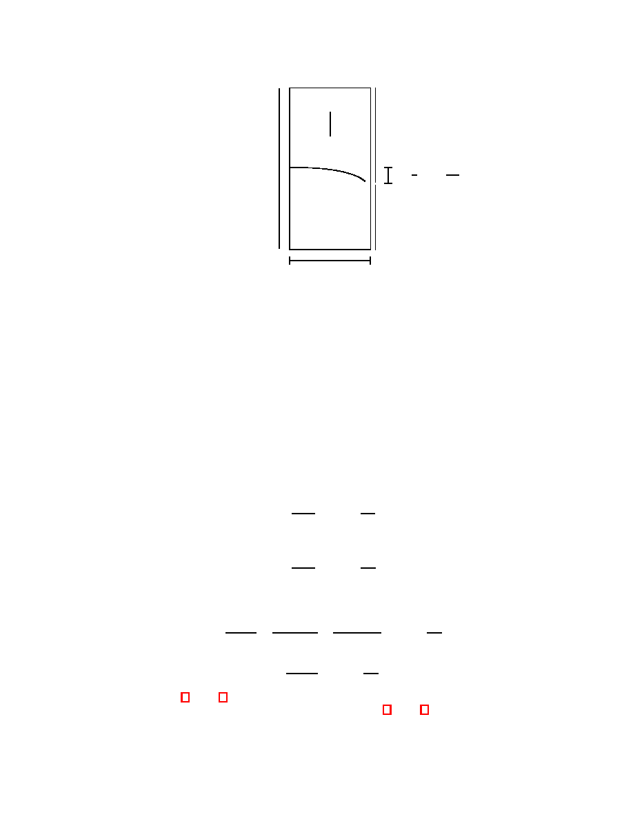
r
B
6
r
B
′
?δ =
1
2
at
2
=
ar
2
2
c
2
A
r
r
C
r
D
s
—
—
6
?
2r
-
r
?
6
6
a
Figure 1
. Three light rays propagate in an accelerating elevator. After having been emitted simultaneously from
points A, C, and D the rays meet at B
′
. The ray propagating from D towards B, but arriving at B
′
, represents
the original thought experiment considered by Einstein. The light rays emitted from A and C are introduced in
order to determine the expressions for the average velocity of light in an accelerating frame of reference.
Consider an elevator accelerating with an acceleration a = |a| which represents a non-inertial (accelerating)
reference frame N
a
(Figure 1). Three light rays are emitted simultaneously in the elevator (in N
a
) from points D,
A, and C toward point B. Let I be an inertial reference frame instantaneously at rest with respect to N
a
(i.e. the
instantaneously comoving frame) at the moment the light rays are emitted. The emission of the rays is therefore
simultaneous in N
a
as well as in I (I and N
a
have a common instantaneous three-dimensional space at this moment
and therefore common simultaneity). At the next moment an observer in I sees that the three light rays arrive
simultaneously not at point B, but at B
′
since for the time t = r/c the light rays travel toward B the elevator moves
at a distance δ = at
2
/2 = ar
2
/2c
2
. As the simultaneous arrival of the three rays at point B
′
as viewed in I is an
absolute (observer-independent) fact due to its being a point event, it follows that the rays arrive simultaneously at
B
′
as seen from N
a
as well. Since for the same coordinate time t = r/c in N
a
the three light rays travel different
distances DB
′
≈ r, AB
′
= r + δ, and CB
′
= r − δ, before arriving simultaneously at point B
′
, an observer in the
elevator concludes that the propagation of light is affected by the elevator’s acceleration. The average velocity c
a
AB
′
of the light ray propagating from A to B
′
is slightly greater than c
c
a
AB
′
=
r + δ
t
≈ c
1 +
ar
2c
2
.
The average velocity c
a
B
′
C
of the light ray propagating from C to B
′
is slightly smaller than c
c
a
CB
′
=
r − δ
t
≈ c
1 −
ar
2c
2
.
It is easily seen that to within terms ∼ c
−2
the average light velocity between A and B is equal to that between A
and B
′
, i.e. c
a
AB
= c
a
AB
′
and also c
a
CB
= c
a
CB
′
:
c
a
AB
=
r
t − δ/c
=
r
t − at
2
/2c
=
c
1 − ar/2c
2
≈ c
1 +
ar
2c
2
(1)
and
c
a
CB
=
r
t + δ/c
≈ c
1 −
ar
2c
2
.
(2)
As the average velocities (1) and (2) are not determined with respect to a specific point and since the coordinate
time t is involved in their calculation, it is clear that the expressions (1) and (2) represent the average coordinate
velocities between the points A and B and C and B, respectively.
8

The same expressions for the average coordinate velocities c
a
AB
and c
a
CB
can be also obtained from the expression
for the coordinate velocity of light in N
a
. If the z-axis is parallel to the elevator’s acceleration a the spacetime
metric in N
a
has the form [39, p. 173]
ds
2
=
1 +
az
c
2
2
c
2
dt
2
− dx
2
− dy
2
− dz
2
.
(3)
Note that due to the existence of a horizon at z = −c
2
/a [39, pp. 169, 172-173] there are constrains on the size of
non-inertial reference frames (accelerated or at rest in a parallel gravitational field) which are represented by the
metric (3). If the origin of N
a
is changed, say to z
B
= 0 (See Figure 1), the horizon moves to z = −c
2
/a − |z
B
|.
As light propagates along null geodesics ds
2
= 0 the coordinate velocity of light at a point z in N
a
is
c
a
(z) = ±c
1 +
az
c
2
.
(4)
The + and − signs are for light propagating along or against z, respectively. Therefore, the coordinate velocity of
light at a point z is locally isotropic in the z direction. It is clear that c
a
(z) cannot become negative due to the
constraints on the size of non-inertial frames which ensure that |z| < c
2
/a [39, pp. 169, 172].
As the coordinate velocity c
a
(z) is continuous on the interval [z
A
, z
B
] one can calculate the average coordinate
velocity between A and B in Figure 1:
c
a
AB
=
1
z
B
− z
A
Z
z
B
z
A
c
a
(z) dz = c
1 +
az
B
c
2
+
ar
2c
2
,
(5)
where we took into account that z
A
= z
B
+ r. When the coordinate origin is at point B (z
B
= 0) the expression (5)
coincides with (1). In the same way:
c
a
BC
= c
1 +
az
B
c
2
−
ar
2c
2
,
(6)
where z
C
= z
B
− r. For z
B
The average coordinate velocities (5) and (6) correctly describe the propagation of light in N
a
yielding the right
expression δ = ar
2
/2c
2
(See Figure 1). It should be stressed that without these average coordinate velocities the
fact that the light rays emitted from A and C arrive not at B, but at B
′
cannot be explained.
As a coordinate velocity, the average coordinate velocity of light is not determined with respect to a specific
point and depends on the choice of the coordinate origin. Also, it is the same for light propagating from A to B
and for light travelling in the opposite direction, i.e. c
a
AB
= c
a
BA
. Therefore, like the coordinate velocity (4) the
average coordinate velocity is also isotropic but only in a sense that the average light velocity between two points
is the same in both directions. As seen from (5) and (6) the average coordinate velocity of light between different
pairs of points, whose points are the same distance apart, is different and this sense it is anisotropic. As a result, as
seen in Figure 1, the light ray emitted at A arrives at B before the light ray emitted at C.
In an elevator supported in a parallel gravitational field (representing a non-inertial reference frame N
g
), where
the metric is [39, p. 1056]
ds
2
=
1 +
2gz
c
2
c
2
dt
2
− dx
2
− dy
2
− dz
2
,
(7)
the expressions for the average coordinate velocity of light between A and B and B and C, respectively, are
c
g
AB
= c
1 +
gz
B
c
2
+
gr
2c
2
and
c
g
BC
= c
1 +
gz
B
c
2
−
gr
2c
2
.
The average coordinate velocity of light explains the propagation of light in the Einstein elevator, but cannot
be used in a situation where the average light velocity between two points (say a source and an observation point)
is determined with respect to one of the points. Such situations occur in the Shapiro time delay [40] and, as we
9
shall see, when one calculates the potential, the electric field, and the self-force of a charge in non-inertial frames of
reference. As the local velocity of light is c the average velocity of light between a source and an observation point
depends on which of the two points is regarded as a reference point with respect to which the average velocity is
determined (at the reference point the local velocity of light is c). The dependence of the average velocity on which
point is chosen as a reference point demonstrates that that velocity is anisotropic. This anisotropic velocity can be
regarded as an average proper velocity of light since it is determined with respect to a given point and its calculation
involves the proper time at that point.
The average proper velocity of light between A and B can be obtained by using the average coordinate velocity
of light (5) between the same points:
c
a
AB
≡
r
∆t
= c
1 +
az
B
c
2
+
ar
2c
2
Let us calculated the average proper velocity of light propagating between A and B as determined from point A.
This means that we will use A’s proper time ∆τ
A
= 1 + az
A
/c
2
∆t:
¯
c
a
AB
(as seen f rom A) ≡
r
∆τ
A
=
r
∆t
∆t
∆τ
A
.
Noting that r/∆t is the average coordinate velocity (5) and z
A
= z
B
+ r we have (to within terms ∼ c
−2
)
¯
c
a
AB
(as seen f rom A) ≈ c
1 +
az
B
c
2
+
ar
2c
2
1 −
az
A
c
2
≈ c
1 −
ar
2c
2
.
(8)
The calculation of the average proper velocity of light propagating between A and B, but as seen from B yields:
¯
c
a
AB
(as seen f rom B) ≡
r
∆τ
B
=
r
∆t
∆t
∆τ
B
≈ c
1 +
az
B
c
2
+
ar
2c
2
1 −
az
B
c
2
≈ c
1 +
ar
2c
2
.
(9)
The average proper velocities (8) and (9) can be derived without using the average coordinate velocity of light.
Consider a light source at point B (Figure 1). As seen from the metric (3) proper and coordinate times do not
coincide whereas proper and coordinate distances are the same [41]. To calculate the average proper velocity of light
originating from B and observed at A (that is, as seen from A) we have to determine what are the initial velocity
of a light signal at B and its final velocity at A both with respect to A. As the local velocity of light is c the final
velocity of the light signal determined at A is also c. Its initial velocity at B as seen from A is
c
a
B
=
dz
B
dτ
A
=
dz
B
dt
dt
dτ
A
where dz
B
/dt = c
a
(z
B
) is the coordinate velocity (4) at B
c
a
(z
B
) = c
1 +
az
B
c
2
and dτ
A
is the proper time at A
dτ
A
=
1 +
az
A
c
2
dt.
As z
A
= z
B
+ r and az
A
/c
2
< 1 for the coordinate time dt we have (to within terms ∼ c
−2
)
dt =
1 −
az
A
c
2
dτ
A
=
1 −
az
B
c
2
−
ar
c
2
dτ
A
.
Then for the initial velocity c
a
B
at B as seen from A we obtain
c
a
B
= c
1 +
az
B
c
2
1 −
az
B
c
2
−
ar
c
2
or keeping only the terms ∼ c
−2
c
a
B
= c
1 −
ar
c
2
.
(10)
10

The initial velocity c
a
B
at B as seen from A is the proper velocity of light at B determined by A. As seen from (10)
this velocity is linear in both distance and time which allows us to determine the average proper velocity of light
between two points by using only the proper velocities of light at those points. Therefore, for the average proper
velocity c
a
BA
= (1/2)(c
a
B
+ c) of light propagating from B to A as seen from A we have
c
a
BA
(as seen f rom A) = c
1 −
ar
2c
2
,
(11)
which coincides with (8).
As the local velocity of light at A is c it follows that if light propagates from A toward B its average proper
velocity c
a
AB
(as seen f rom A) will be equal to the average proper velocity of light propagating from B toward A
c
a
BA
(as seen f rom A). Thus, as seen from A, the back and forth average proper velocities of light travelling between
A and B are the same.
Now let us determine the average proper velocity of light between B and A with respect to the source point B.
A light signal emitted at B as seen from B will have an initial (local) velocity c there. The final velocity of the
signal at A as seen from B will be
c
a
A
=
dz
A
dτ
B
=
dz
A
dt
dt
dτ
B
where dz
A
/dt = c
a
(z
A
) is the coordinate velocity at A
c
a
(z
A
) = c
1 +
az
A
c
2
and dτ
B
is the proper time at B
dτ
B
=
1 +
az
B
c
2
dt.
Then as z
A
= z
B
+ r we obtain for the velocity of light c
a
A
at A as determined from B
c
a
A
= c
1 +
ar
c
2
and the average proper velocity of light propagating from B to A as seen from B becomes
c
a
BA
(as seen f rom B) = c
1 +
ar
2c
2
.
(12)
As expected (12) coincides with (9).
Comparing (11) and (12) demonstrates that the two average proper velocities between the same points are not
equal and depend on from where they are seen. As we expected the fact that the local velocity of light at the
reference point is c makes the average proper velocity between two points dependant on where the reference point
is.
In order to express the average proper velocity of light in a vector form (which will turn out to be helpful for the
calculation of the electric field in the next section) let the light emitted from B be observed at different points. The
average proper velocity of light emitted at B and determined at A (Figure 1) is given by (11). As seen from point
C the average proper velocity of light from B to C will be given by the same expression as (12)
c
a
BC
(as seen f rom C) = c
1 +
ar
2c
2
.
As seen from a point P at a distance r from B and lying on a line forming an angle θ with the acceleration a) the
average proper velocity of light from B is
c
a
BP
(as seen f rom P ) = c
1 −
ar cos θ
2c
2
.
Then the average proper velocity of light coming from B as seen from a point defined by the position vector r
originating from B has the form
¯
c
a
= c
1 −
a
· r
2c
2
.
(13)
11

As evident from (13) the average proper velocity of light emitted from a common source and determined at
different points around the source is anisotropic in N
a
- if the observation point is above the light source (with
respect to the direction of a) the average proper velocity of light is slightly smaller than c and smaller than the
average proper velocity as determined from an observation point below the source. If an observer at point B (Figure
1) determines the average proper velocities of light coming from A and C he will find that they are also anisotropic
- the average proper velocity of a light signal coming from A is slightly greater than that emitted at C and therefore
the A-signal will arrive first. However, if the observer at B (Figure 1) determines the average proper velocities of
light propagating between A and B and B and A he finds that the two average proper velocities are the same.
The calculation of the average proper velocity of light in the frame N
g
of an observer supported in a parallel
gravitational field can be obtained in the same way and the resulting expression is:
¯
c
g
= c
1 +
g
· r
2c
2
,
(14)
where g is the gravitational acceleration. It is interesting to note that a substitution of a = −g in (13) yields (14) as
required by the principle of equivalence. The next section will offer us an additional reason to look into the question
whether this result is an indication that the identical anisotropic velocities of light in N
a
and N
g
may provide us
with an insight into what lies behind the equivalence principle.
The velocities (13) and (14) demonstrate that there exists a directional dependence in the propagation of light
between two points in non-inertial frames of reference (accelerating or at rest in a gravitational field). This anisotropy
in the propagation of light has been an overlooked corollary of general relativity. In fact, up to now neither the
average coordinate velocity nor the average proper velocity of light have been defined. However, we have seen that
the average coordinate velocity is needed to account for the propagation of light in non-inertial reference frames (to
explain the fact that two light signals emitted from points A, and C in Figure 1 meet at B
′
, not at B). We will also
see below that the average proper velocity is necessary for the correct description of electromagnetic phenomena in
non-inertial frames in full accordance with the equivalence principle.
5
Electromagnetic mass theory and anisotropic velocity of light
Here we shall not follow the standard approach to calculating the self-force [34], [44]-[46] which describes an electron’s
accelerated motion in an inertial frame I. Instead, all calculations will be carried out in the non-inertial reference
frame N
a
in which the accelerating electron is at rest. The reason for this is that the calculation of the electric
field and the self-force of an accelerating electron in the accelerating frame N
a
(not in I) is crucial for the correct
application of the principle of equivalence since it relates those quantities of an electron in a non-inertial (accelerating)
frame N
a
and in a non-inertial frame N
g
supported in a gravitational field. An advantage of calculating the electron’s
electric field in the non-inertial frame in which the electron is at rest is that it is obtained only from the scalar potential
and the calculations do not involve retarded times.
5.1
An electron in a non-inertial (accelerating) reference frame N
a
In the case of an accelerating reference frame the anisotropic velocity of light (13) leads to two changes in the
potential
dϕ
a
= −
ρdV
a
4πǫ
o
r
a
,
(15)
of an electron at rest in N
a
and described there as compared to the standard Coulomb potential of an inertial
electron determined in its rest frame, where −ρ is the density of the electron charge, r
a
is the distance between the
charge element −ρdV
a
and the observation point, and dV
a
is an anisotropic volume element of the electron charge
(to be defined later) both determined in N
a
.
First, analogously to determining the distance between a charge and an observation point as r = ct (where t
is the time it takes for an electromagnetic signal to travel from the charge to the point at which the potential is
determined) in an inertial reference frame [34, p. 416], r
a
is expressed in N
a
as r
a
= ¯
c
a
t. Since a · r/2c
2
< 1 we can
write
(r
a
)
−1
≈ r
−1
1 +
a
· r
2c
2
.
(16)
12

The second change in (15) is a Li´enard-Wiechert-like (or rather anisotropic) volume element dV
a
(not coinciding
with the actual volume element dV ) which arises in N
a
on account of the anisotropic velocity of light there. The
origin of dV
a
is analogous to the origin of the Li´enard-Wiechert volume element dV
LW
= dV / (1 − v · n/c) of a
charge moving at velocity v with respect to an inertial observer I, where n = r/r and r is the position vector at the
retarded time [34, p. 418]. The origin of dV
LW
can be explained in terms of the ”information-collecting sphere” of
Panofsky and Phillips [45, p. 342] used in the derivation of the Li´enard-Wiechert potentials; similar concepts are
employed by Feynman [25, p. 21-10], Griffiths [34, p. 418], and Schwartz [47].
A charge approaching an observation point where the potential is determined contributes more to the potential
there ”than if the charge were stationary” [47, p. 215] since it ”stays longer within the information-collecting
sphere” [45, p. 343] which converges toward the observation point and therefore chases the charge at the velocity
of light c in I. The greater contribution to the potential may be viewed as originating from a charge of a Li´enard-
Wiechert volume dV
LW
that appears greater than dV [48]. If the charge is receding from the observation point,
the information-collecting sphere moves against the charge, the charge stays less within it and the resulting smaller
contribution of the charge to the potential appears to come from a charge whose Li´enard-Wiechert volume dV
LW
appears smaller than dV .
By the same argument the anisotropic volume dV
a
also appears different from dV in N
a
. Consider a charge of
length l (placed in a direction parallel to a) at rest in N
a
. The time for which the information-collecting sphere
traveling at the average velocity of light (13) in N
a
sweeps over the charge is
∆τ
a
=
l
¯
c
a
=
l
c (1 − a · r/2c
2
)
≈ ∆t
1 +
a
· r
2c
2
,
where ∆t = l/c is the time for which the information-collecting sphere propagating at speed c sweeps over an inertial
charge of the same length l in its rest frame. If the observation point where the potential is determined is above the
charge (in a direction parallel to a), the information-collecting sphere moves along a in N
a
, its average velocity is
slightly smaller than c (as seen from that point) and therefore ∆τ
a
> ∆t (since a · r = ar). As a result the charge
stays longer within the sphere and its contribution to the potential is greater. This is equivalent to saying that the
greater contribution comes from a charge of a greater length l
a
which for the same time ∆τ
a
is swept over by an
information-collecting sphere propagating at velocity c:
l
a
= ∆τ
a
c = l
1 +
a
· r
2c
2
.
If the point where the potential is determined is below the charge, the information-collecting sphere moves against a
in N
a
(meaning that a · r = −ar), its average velocity is slightly greater than c (as seen from the observation point)
and the time for which the sphere moves over the charge is smaller: ∆τ
a
< ∆t. Therefore the charge stays less time
within the information-collecting sphere and its contribution to the potential is smaller which can be interpreted to
mean that a charge of a shorter length is making a smaller contribution to the potential.
The anisotropic volume element which corresponds to such an apparent length l
a
is obviously
dV
a
= dV
1 +
a
· r
2c
2
.
(17)
The scalar potential of a charged volume element −ρdV
a
of the electron at rest in N
a
can now be calculated by
substituting (16) and (17) in (15)
dϕ
a
= −
1
4πǫ
0
ρdV
a
r
a
= −
1
4πǫ
0
ρdV
r
1 +
a
· r
2c
2
2
or keeping only the terms proportional to c
−2
we obtain
dϕ
a
= −
ρ
4πǫ
0
r
1 +
a
· r
c
2
dV.
(18)
The electric field of the charged volume element −ρdV
a
can be calculated only from the scalar potential (18) without
the involvement of retarded times since the charged element is at rest in N
a
dE
a
= −∇dϕ
a
= −
1
4πǫ
o
n
r
2
+
a
· n
c
2
r
n
−
a
c
2
r
ρdV.
13
The electric field of the electron then is
E
a
= −
1
4πǫ
o
Z
n
r
2
+
a
· n
c
2
r
n
−
a
c
2
r
ρdV.
(19)
If we compare the electric field (19) of an electron at rest in N
a
(determined in N
a
) and its field [44, p. 664]
determined in an inertial reference frame I in which the electron is instantaneously at rest we see that for both an
observer in N
a
and an observer in I the electron’s field is equally distorted. Therefore, as we expected it does turn
out that the shape of the electric field of an accelerating charge is absolute like acceleration itself. This implies that
there exists a correspondence between the shape of a charge and its state of motion which is observer-independent.
As for all observers (both inertial and non-inertial) a worldline is either geodesic or not, the field of an inertial charge
represented by a geodesic worldline is the Coulomb field, whereas the field of a non-inertial charge (accelerating or,
as we shall see below, supported in a gravitational field) whose worldline is not geodesic is distorted.
The self-force which the field of the electron exerts upon an element −ρdV
a
1
of its own charge is
dF
a
self
= −ρdV
a
1
E
a
=
1
4πǫ
o
Z
n
r
2
+
a
· n
c
2
r
n
−
a
c
2
r
ρ
2
dV dV
a
1
.
(20)
The resultant self-force acting on the electron as a whole is:
F
a
self
=
1
4πǫ
o
Z
Z
n
r
2
+
a
· n
c
2
r
n
−
a
c
2
r
ρ
2
dV dV
a
1
,
(21)
which after taking into account the anisotropic volume element (17) becomes
F
a
self
=
1
4πǫ
o
Z
Z
n
r
2
+
a
· n
c
2
r
n
−
a
c
2
r
1 +
a
· r
2c
2
ρ
2
dV dV
1
.
Assuming a spherically symmetric distribution of the electron charge [9] and following the standard procedure
of calculating the self-force [46] we get (see Appendix):
F
a
self
= −
U
c
2
a
,
(22)
where
U =
1
8πǫ
o
Z
Z
ρ
2
r
dV dV
1
is the energy of the electron’s electric field. As U/c
2
is the mass that corresponds to that energy we can write (22)
in the form:
F
a
self
= −m
a
a
,
(23)
where m
a
= U/c
2
is identified as the electron inertial electromagnetic mass. The famous factor of 4/3 in the
electromagnetic mass of the electron does not appear in (23). The reason is that in (20) and (21) we have identified
and used the correct volume element dV
a
1
= 1 + a · r/2c
2
dV
1
originating from the anisotropic velocity of light in
N
a
; not taking it into account results in the appearance of the 4/3 factor.
The self-force F
a
self
to which an electron is subjected due to its own distorted field is directed opposite to a and
therefore resists the acceleration of the electron. As seen from (22) this force is purely electromagnetic in origin and
therefore both the resistance the classical electron offers to being accelerated (i.e. its inertia) and its inertial mass
(which is a measure of that resistance) are purely electromagnetic in origin as well.
The self-force (23) is traditionally called the inertial force. According to Newton’s third law the external force F
that accelerates the electron and the self-force F
a
self
which resists F have equal magnitudes and opposite directions:
F
= −F
a
self
. Therefore we can write F = m
a
a
which means that Newton’s second law can be derived on the basis
of Maxwell’s electrodynamics applied to the classical model of the electron and Newton’s third law.
We have seen that the average anisotropic velocity of light in N
a
causes the imbalance in the repulsion of all
volume elements −ρdV
a
and −ρdV
a
1
that is responsible for the self-force F
a
self
to which an electron as a whole is
subjected and which resists its accelerated motion. While it is the net effect of the unbalanced repulsion of the
electron volume elements that gives rise to its electromagnetic mass, the contribution to the mass of the unbalanced
14
repulsion of individual charges is more complex. The unbalanced repulsion of two like charges whose line of interaction
is perpendicular to the acceleration a increases their mass. The unbalanced repulsion of two charges whose line of
interaction is parallel to a, however, decreases their mass as can be verified by direct calculation. By taking into
account the anisotropic volume element dV
a
1
in (20) the latter effect has resulted in reducing the electron mass from
4/3 m to m.
If the unbalanced repulsion of like charges causes the classical electron’s inertia, mass, and the self-force F
a
self
that acts in a direction opposite to a, it is quite natural to ask what the effect of the unbalanced attraction of two
unlike charges −ρdV
a
and +ρdV
a
1
will be. As in the case of unbalanced repulsion it depends on the angle between a
and the line of interaction of the two opposite charges. The unbalanced attraction of two charges −ρdV
a
and +ρdV
a
1
whose line of interaction is perpendicular to the acceleration a decreases their mass by dm since the self-force acting
on them is in the direction of a: dF
a
self
= dma. This is an inevitable but nevertheless a surprising result since it
demonstrates that not only does the self-force acting on accelerating opposite charges not resist their acceleration
but further increases it [50], [51] (note that this effect is different from the runaway problem [52] in the classical
electron theory). On the other hand, the negative contribution to the mass resulting from unbalanced attraction is
not so surprising - in Section 3 we have seen that non-electric attraction forces also make a negative contribution to
the mass. When the line of interaction of two opposite charges is parallel to a their unbalanced attraction increases
their mass since the self-force in this case is dF
a
self
= − dma.
Let us now calculate the electric field of an inertial electron whose charge is e and which appears falling in
N
a
with an apparent acceleration a
∗
= −a (where a is the acceleration of N
a
). It is obvious that for an inertial
observer I falling with the electron its electric field is the Coulomb field. In order to obtain the electric field of the
falling electron in N
a
we have to use generalized Li´enard-Wiechert potentials which take into account the anisotropic
velocity of light in N
a
. These can be directly obtained by replacing r with r
a
and the actual volume element dV with
the anisotropic volume element dV
a
in the expressions for the Li´enard-Wiechert potentials in an inertial reference
frame:
ϕ
a
(r, t) =
−
e
4πǫ
o
r
1
1 − v · n/c
1 +
a
· r
c
2
ret
(24)
A
a
(r, t) =
−
e
4πǫ
o
c
2
r
v
1 − v · n/c
1 +
a
· r
c
2
ret
,
(25)
where, as usual, the subscript ”ret” indicates that the quantity in the square brackets is evaluated at the retarded
time. The electric field of an electron falling in N
a
(and considered instantaneously at rest in N
a
) obtained from
E
= −∇ϕ
a
−
∂A
a
∂t
= −
e
4πǫ
o
n
r
2
+
a
∗
·n
c
2
r
n
−
a
∗
c
2
r
+
a
· n
c
2
r
n
−
a
c
2
r
.
Noting that a
∗
= −a it proves that the electric field of the falling electron, as described in N
a
, is identical with the
field of an inertial electron determined in its rest frame:
E
= −
e
4πǫ
o
n
r
2
.
This result shows that for a non-inertial observer at rest in N
a
the instantaneous electric field of the falling electron
is the Coulomb field. Therefore, the assumption that the shape of the electric field of an inertial electron is absolute
is also confirmed since both I and N
a
detect a Coulomb field of the falling electron. In general: (i) a Coulomb field
is associated with an inertial electron (represented by a geodesic worldline) by both an inertial observer I (moving
with the electron) and a non-inertial observer N
a
, and (ii) for both I and N
a
the electric field of a non-inertial
electron (whose worldline is not geodesic) is equally distorted. As we expected the fact that the state of (inertial or
accelerated) motion of a charge is absolute implies that the shape of the electric field of an (inertial or accelerated)
charge is also absolute (the same for an inertial and a non-inertial observer).
15
5.2
An electron in a non-inertial reference frame N
g
at rest in the Earth’s gravita-
tional field
Similarly to the case of calculating the electric potential in N
a
the average anisotropic velocity of light (14) in N
g
also leads to anisotropic r
g
and dV
g
in N
g
:
(r
g
)
−1
≈ r
−1
1 −
g
· r
2c
2
and
dV
g
= dV
1 −
g
· r
2c
2
.
(26)
As a result the scalar potential of a charged volume element −ρdV
g
of the electron in N
g
is:
dϕ
g
= −
ρ
4πǫ
0
r
1 −
g
· r
c
2
dV.
(27)
It should be emphasized that only by taking into account the anisotropic volume element dV
g
we can obtain the
correct potential (27) of a charge supported in a gravitational field. By using the actual volume element dV in 1921
Fermi [11] derived the expression
ϕ =
e
4πǫ
0
r
1 −
1
2
gz
c
2
(28)
for the potential of a charge at rest in a gravitational field. The use of dV resulted in the factor 1/2 in the parenthesis
which leads to a contradiction with the principle of equivalence when the electric field is calculated from this potential:
it follows from (28) that the electric field of a charge supported in the Earth’s gravitational field coincides with the
instantaneous electric field of a charge moving with an acceleration a = −g/2 (obviously the principle of equivalence
requires that a = −g).
The calculation of the electric field of a charged volume element −ρdV
g
in N
g
is again carried out by using only
the scalar potential (27):
dE
g
= −∇dϕ
g
= −
1
4πǫ
o
n
r
2
−
g
· n
c
2
r
n
+
g
c
2
r
ρdV
and the field of the electron is then
E
g
= −
1
4πǫ
o
Z
n
r
2
−
g
· n
c
2
r
n
+
g
c
2
r
ρdV.
(29)
A comparison of the electric field of an electron supported in the Earth’s gravitational field (29), determined in N
g
,
with the electric field of an accelerated electron (19), determined in the frame N
a
, indicates that the electric fields of
an electron at rest on the Earth’s surface and an electron at rest in the frame N
a
which moves with an acceleration
a
= −g are equally distorted in accordance with the principle of equivalence. A substitution a = −g in (18) also
transforms it into (27) as required by the equivalence principle.
The self-force with which the electron field interacts with an element −ρdV
g
1
of the electron charge is therefore
dF
g
self
= −ρdV
g
1
E
g
=
1
4πǫ
o
Z
n
r
2
−
g
· n
c
2
r
n
+
g
c
2
r
ρ
2
dV dV
g
1
(30)
and the resultant self-force with which the electron acts upon itself is:
F
g
self
=
1
4πǫ
o
Z
Z
n
r
2
−
g
· n
c
2
r
n
+
g
c
2
r
ρ
2
dV dV
g
1
,
(31)
After taking into account the explicit form (26) of dV
g
1
, assuming a spherically symmetric distribution of the electron
charge, and calculating the self-force as we have done in the case of an electron at rest in N
a
we get:
F
g
self
=
U
c
2
g
,
(32)
where
16

U =
1
8πǫ
o
Z
Z
ρ
2
r
dV dV
1
is the energy of the electron’s field. As U/c
2
is the mass associated with the field energy of the electron, i.e. its
electromagnetic mass, (32) obtains the form:
F
g
self
= m
g
g
,
(33)
where m
g
= U/c
2
is interpreted here as the electron passive gravitational mass. As in the case of the self-force acting
on an accelerating electron described in N
a
the 4/3 factor in the electromagnetic mass does not appear in (33) for
the same reason: the correct volume element (26) was used in (31). Therefore the anisotropic volume element dV
g
simultaneously resolves two different problems - removes both the 1/2 factor in the potential (28) derived by Fermi
and the 4/3 factor in the self-force.
The self-force F
g
self
which acts upon an electron on account of its own distorted field is directed parallel to g
and resists the deformation of its electric field caused by the fact that the electron at rest on the Earth’s surface is
prevented from falling. This force is traditionally called the gravitational force. As we have seen F
g
self
arises only
when an electron is prevented from falling, i.e. only when it is deviated from its geodesic path. Only in this case
the electron field deforms which gives rise to the self-force F
g
self
. Thus F
g
self
resists the deformation of the field of
the electron which means that it resists its being prevented from following a geodesic path. As a Coulomb field is
associated with a non-resistantly moving electron (represented by a geodesic worldline) it follows that F
g
self
is, in
fact, an inertial force since it resists the deviation of an electron from its geodesic path, that is, F
g
self
resists the
deviation of the electron from its motion by inertia. Therefore, the nature of the force acting upon an electron at
rest in a gravitational field is inertial and is purely electromagnetic in origin as seen from (33), which means that
the electron passive gravitational mass m
g
in F
g
self
= m
g
g
is also purely electromagnetic in origin. It is immediately
clear from here why the inertial and the passive gravitational masses of the classical electron are equal. As the nature
of the self-force F
g
self
is inertial it follows that what is traditionally called passive gravitational mass is, in fact, also
inertial mass. This becomes evident from the fact that the two masses are the measure of resistance an electron offers
when deviated from its geodesic path. In flat spacetime the force of resistance is F
a
self
= −m
a
a
whereas in curved
spacetime this same force that resists the deviation of the electron from its geodesic path is F
g
self
= m
g
g
where m
a
and m
g
are the measures of resistance (inertia) in both cases. The two resistance force are equal F
a
self
= F
g
self
for
a = g as seen from (22) and (32) and therefore m
a
= m
g
. This equivalence also follows from the fact that m
a
and
m
g
are the same thing - the mass associated with the energy of the electron field.
The result that the force F
g
self
, acting on an electron when it is deviated from its geodesic path due to its being at
rest in a gravitational field, is inertial is valid not only for the classical electron. A non-resistant motion (i.e. motion
by inertia) of a body in both special relativity (flat spacetime) and general relativity (curved spacetime) is represented
by a geodesic worldline whereas a body represented by a non-geodesic worldline is subjected to a resistance force
which opposes the external force preventing the body from following its geodesic path in spacetime. That is why
the nature of the resistance force is inertial in both special and general relativity. It should be specifically stressed
here that the conclusion of the non-gravitational nature of the force acting on a body at rest in a gravitational
field follows from general relativity itself [42, p. 244]: as a body supported in a gravitational field is deviated from
its geodesic path, which means that it is prevented from moving non-resistantly (by inertia), it is subjected to an
inertial force since it arises only when the body is prevented from moving in a non-resistant (inertial) manner. This
explains why in general relativity ”there is no such thing as the force of gravity” [53].
As seen from (30) it is the unbalanced repulsion of all volume elements −ρdV
g
and −ρdV
g
1
(caused by the average
anisotropic velocity of light in N
g
) that is responsible for the self-force F
g
self
to which the electron as a whole is
subjected (if the velocity of light were isotropic, all forces of repulsion of the electron volume elements would cancel
out and there would be no self-force acting upon the electron as a whole). As in the acceleration case here too
the unbalanced attraction of two unlike charges −ρdV
g
and +ρdV
g
1
changes the sign in the self-force in (30), which
means that for the case when the line of interaction of the charges is perpendicular to g it becomes a levitation
force [54], [51] whose effect is to reduce the charges’ passive gravitational electromagnetic mass. The unbalanced
attraction of unlike charges whose line of interaction is parallel to g results in a self-force in the direction of g which
increases their mass. In a gravitational field, the unbalanced repulsion of two like charges interacting along a line
17
perpendicular to g produces a self-force parallel to g. The self-force produced by the unbalanced repulsion of the
like charges interacting along a line parallel to g is opposite to g.
Let us now calculate the electric field of an electron falling in the Earth’s gravitational field. General relativity
describes an electron falling in a gravitational field by a geodesic worldline. It implies that it moves by inertia
(without resistance) and its Coulomb field is not distorted for an inertial observer I falling with the electron. In
order to obtain the electric field of an electron falling with acceleration a = g in the Earth’s gravitational field (in
N
g
) we have to use the generalized Li´enard-Wiechert potentials which include the corrections due to the average
anisotropic velocity of light in N
g
as we have done in the case of an electron falling in N
a
. Their explicit expressions
in N
g
are:
ϕ
g
(r, t) =
−
e
4πǫ
o
r
1
1 − v · n/c
1 −
g
· r
c
2
ret
(34)
A
g
(r, t) =
−
e
4πǫ
o
c
2
r
v
1 − v · n/c
1 −
g
· r
c
2
ret
.
(35)
The electric field of the electron falling in N
g
(and considered instantaneously at rest in N
g
) obtained from (34)
and (35) is:
E
= −∇ϕ
g
−
∂A
g
∂t
= −
e
4πǫ
o
h
n
r
2
+
g
· n
c
2
r
n
−
g
c
2
r
+
−
g
· n
c
2
r
n
+
g
c
2
r
i
.
Therefore the electric field of the falling electron in the reference frame N
g
proves to be identical with the field of
an inertial electron determined in its rest frame:
E
= −
e
4πǫ
o
n
r
2
.
(36)
As seen from (36) while the electron is falling in the Earth’s gravitational field its electric field at any instant is
the Coulomb field which means that no self-force is acting on the electron, i.e. there is no resistance to its accelerated
motion. This explains why the electron is falling in a gravitational field by itself and no external force is causing its
acceleration. As (36) shows, the only way for the electron to compensate the anisotropy in the propagation of light
and to preserve the Coulomb shape of its electric field is to fall with an acceleration g. If the electron is prevented
from falling its electric field distorts, the self-force (33) appears and tries to force the electron to move (fall) in such
a way that its field becomes the Coulomb field; as a result the self-force disappears.
The result that the electron (and any charge) falls in a gravitational field with an acceleration g by itself in order
to prevent its field from getting distorted may shed light on two facts: (i) that in general relativity the motion of
a body falling toward a gravitating center is regarded as inertial (non-resistant) and is represented by a geodesic
worldline, and (ii) the experimental fact that all objects fall in a gravitational field with the same acceleration.
The conclusion that the electron preserves the Coulomb shape of its field while falling in a gravitational field
is also quite relevant to the debate [18], [55]-[58] on whether or not a falling charge radiates. As (36) shows the
electric field of a falling charge is the Coulomb field and therefore does not contain the radiation r
−1
terms - this is
a straightforward demonstration that a charge falling in a gravitational field does not radiate [49].
The result (36) demonstrates the important fact that a Coulomb field is associated with the falling electron by
both an inertial observer I (falling with the electron) and a non-inertial observer at rest in N
g
. This again confirms
the assumption that the shape of the electric field of an inertial electron (represented by a geodesic worldline) is
absolute (observer-independent) due to the fact that the inertial motion is itself absolute.
Now we are in a position to answer all four questions formulated in Section 3. (i) An electron moving with constant
velocity in a flat spacetime region where the average velocity of light is isotropic does not resist its uniform motion
since uniform motion (represented by a straight geodesic worldline) in flat spacetime ensures that the electron’s
electric field is the Coulomb field. Stated another way, the only way for an electron to prevent its electric field from
distorting in flat spacetime is to move with constant velocity. (ii) An accelerating electron resists its acceleration
in flat spacetime because the accelerated motion distorts the electron’s electric field which results in an electric
self-force that opposes the deformation of the electron’s field. (iii) An electron falling toward the Earth’s surface
does not resists its (flat-spacetime) acceleration since, as we have seen, falling with an acceleration g is the only
way for the electron to compensate the anisotropy in the propagation of light in the Earth’s vicinity and to prevent
its electric field from getting distorted (the curved-spacetime acceleration of the falling electron is zero). (iv) An
electron at rest on the Earth’s surface is subjected to an electric self-force trying to make the electron fall since the
18

average anisotropic velocity of light in the Earth’s gravitational field distorts the electron field which in turn gives
rise to the self-force. The nature of that force is inertial (not gravitational) and is electromagnetic in origin.
The mechanism giving rise to the free (non-resistant) fall of the electron in a gravitational field and to the
self-force (33) that resists its prevention from falling is identical to the mechanism responsible for the self-force (22)
an accelerated electron in flat spacetime is subjected to and for its free fall as described in the accelerated frame
N
a
. This mechanism implies that the common anisotropy in the propagation of light in N
a
and N
g
gives rise to
similar phenomena whose mathematical expressions transform into one another when the substitution a = −g is
used. Therefore, the equivalence principle seems to originate from the same metrics (3) and (7) which give rise to the
anisotropic propagation of light in the non-inertial frames of reference N
a
and N
g
and to identical electromagnetic
phenomena in N
a
and N
g
.
5.3
Gravitational interaction of the classical electron
We have shown that the inertial and passive gravitational masses of the classical electron are entirely electromagnetic
in origin. As all three masses - inertial, passive gravitational, and active gravitational - are considered equal [59], it
follows that the electron active gravitational mass is fully electromagnetic in origin as well. And since it is only the
charge of the classical electron that represents it (there is no mechanical mass), it follows that the active gravitational
mass of the electron is represented by its charge. Therefore it is the electron charge that distorts spacetime and
causes the average anisotropic velocity of light in the electron’s neighborhood.
We have seen that it is the anisotropy in the average proper velocity of light and the electromagnetic mass theory
that fully and consistently explain the fall of an electron toward the Earth and the self-force acting on an electron
at rest on the Earth’s surface. Let us now see whether the gravitational attraction between two electrons can be
explained in the same way.
In addition to the electric repulsion of two electrons (e
1
and e
2
) in space, they also attract each other through the
anisotropy in the average proper velocity of light caused by each of them: e
1
falls toward e
2
in order to compensate
the anisotropy caused by e
2
and to prevent its electric field from getting distorted and vice versa. In other words, the
charge of the electrons affects the propagation of light around them which in turn changes the shape of the electrons’
worldlines resulting in their convergence toward each other. Therefore, in the framework of the electromagnetic
mass theory the anisotropy in the propagation of light in the electrons’ vicinity is sufficient to explain the electrons’
(gravitational) attraction in terms of non-resistant motion which is not caused by a force. In such a way, as we have
seen above, the case of the classical electron may provide an insight into the question of why no force is involved in
the gravitational attraction of bodies as described by general relativity.
6
Looking for the origin of inertia in QFT
As discussed in the Introduction the same mechanism that accounts for inertia and mass of the classical electron -
the interaction of the electron charge with its distorted field - appears to lead to contributions from all interactions
to the inertia and mass in the framework of QFT.
Consider a free particle, whose constituents are subjected to electromagnetic, weak, and strong interactions. The
recoils the particle suffers due to the emission and absorption of the virtual quanta of the electromagnetic, weak,
and strong ”fields” of its own constituents cancel out precisely. However, it has been overlooked that the recoils from
the virtual quanta absorbed by a non-inertial particle do not cancel - owing to the general relativistic directional
dependency of the frequencies of the incoming virtual quanta (constituting a distortion of the corresponding ”fields”)
the magnitudes of their momenta and therefore the recoils acting on the particle are also direction dependent. That
imbalance in the recoils gives rise to a self-force which is electromagnetic, weak, and strong in origin and which acts
on the non-inertial particle. As this self-force arises only when the particle is prevented from following a geodesic
path it is clearly inertial.
At the conceptual level it appears certain that QFT does say something important about the origin of inertia
and mass - if one believes in the Standard Model they should agree that the recoils from all incoming (blue or red
shifted) virtual quanta absorbed by the electric, weak, and strong non-inertial charges will not cancel out and will
give rise to an inertial force. However, a conceptual analysis does not constitute a real result in physics.
19
What is not only difficult, but almost hopeless is how one can calculate the self-force originating from the
unbalanced recoils from the virtual quanta that are absorbed by a non-inertial particle. There are too many
unknowns. Virtual quanta are off mass shell particles which means that their energy, momentum and mass do
not obey the relativistic equation:
E
2
= p
2
c
2
+ mc
2
2
.
For example, unlike the momentum of a normal photon which is given by p = E/c, the momentum of a virtual
photon is not equal to E/c. Also unknown are the energy of a charge (electromagnetic, weak, or strong) in terms of
the energies of the virtual quanta that constitute the ”field” of the charge, the lifetimes and energies of individual
virtual quanta, and the absorption time during which a virtual quant is absorbed by the charge.
An attempt to overcome those difficulties is to carry out a semiclassical calculation of the self-force in the case
of electromagnetic interaction in QED; similar calculations can be done for the other interactions. For this purpose
the following assumptions will be made. It appears natural to define the energy of the electric field of a charge in
QED as the sum of the energies of all virtual photons constituting the ”field” at a given moment. Such a definition
avoids the issue of the dimension of the charge. In order to eliminate some of the unknowns mentioned above it
appears that an equivalent definition of the charge’s ”field” energy is also possible in terms of the total energy of
the number of virtual photons absorbed by the charge during some characteristic time δt (δt can be regarded as the
time for which the charge renews its ”field”). The lifetimes of all virtual photons can be expressed in terms of δt
as αδt, where α is a real number. The distances travelled by the virtual photons during their lifetimes will be then
αr = αcδt, where r = cδt, is obviously the distance travelled by a virtual photon for the characteristic time δt. The
time for which a virtual photon is absorbed by a charge is assumed to be δτ . The momentum of a virtual photon
can be considered to be p
a
= β (E
a
/c), where β is also a real number and E
a
is the blue/red shifted energy of the
virtual photon being absorbed by an accelerating charge; E
a
is determined in the accelerating reference frame N
a
in which the charge is at rest.
In N
a
the frequency of a virtual photon coming from a given directions toward the charge (as seen by the charge)
can be written in the vector form
f
a
= f
1 −
a
· r
c
2
.
(37)
Here f is the frequency measured at r = 0 and r = nr, where n is a unit vector pointing towards the charge and
determining the direction of the incoming virtual photon.
By the uncertainty principle the energy of a virtual photon of lifetime δt in N
a
is ∆E
a
∼h/δt. A virtual photon
of lifetime αδt will have energy ∆E
a
α
∼h/αδt = ∆E
a
/α. By (37) the energy of this virtual photon can be written as
∆E
a
α
=
∆E
a
α
=
hf
a
α
=
hf
α
1 −
a
· r
c
2
α
=
∆E
α
1 −
a
· r
c
2
α
,
where ∆E/α = hf /α is the energy of that virtual photon determined at r = 0. The momentum of the virtual
photon will be then
∆p
a
αβ
= β
∆E
a
α
c
= β
∆E
a
cα
=
∆Eβ
cα
1 −
a
· r
c
2
α
.
Assume that the number of virtual photons coming from a direction n within the solid angle dΩ which are
absorbed during the characteristic time δt is x. The momentum of all virtual photons x is then
x
X
i=1
∆p
a
α
i
β
i
n
dΩ =
x
X
i=1
∆E
a
β
i
cα
i
n
dΩ =
x
X
i=1
∆Eβ
i
cα
i
1 −
a
· r
c
2
α
i
n
dΩ.
The force produced by the recoils from all x virtual photons is
dF
a
self
=
x
X
i=1
∆p
a
α
i
β
i
δτ
n
dΩ.
20
Then the self-force that acts on the charge and results from the unbalanced recoils of all virtual photons absorbed
during the characteristic time δt and coming from all directions towards the charge is
F
a
self
=
Z
x
X
i=1
∆p
a
α
i
β
i
δτ
n
dΩ =
Z
x
X
i=1
∆Eβ
i
cδτ α
i
1 −
a
· r
c
2
α
i
n
dΩ
=
Z
x
X
i=1
∆Eβ
i
cδτ α
i
n
dΩ −
Z
x
X
i=1
∆Eβ
i
c
3
δτ
(a · r) n dΩ.
(38)
Due to symmetry, the first integral in (38) is zero. Noticing that r = nr and r = cδt, for the self-force we can write
F
a
self
= −
x
X
i=1
∆Eβ
i
δt
c
2
δτ
Z
(a · n) n dΩ.
(39)
The integral in (39) is similar to the one calculated in the Appendix:
Z
(a · n) n dΩ =
4π
3
a
.
By substituting this result in (39) and taking into account that
U = 4π
x
X
i=1
∆Eβ
i
is the total energy of all virtual photons (coming from all directions of the solid angle 4π) absorbed during the time
δt, we obtain for the self-force
F
a
self
= −
1
3
δt
δτ
U
c
2
a
.
The energy U represents the energy of the ”field” of the charge. Therefore the quantity U/c
2
is the mass corresponding
to the energy of the electric ”field” of the charge and can be regarded as its electromagnetic mass m
a
= U/c
2
. If
the characteristic time δt is three times greater than the absorption time δτ , the expression for the self-force acting
on the accelerating charge will have the exact form of the inertial force
F
a
self
= −m
a
a
.
(40)
Despite the fact that the calculations are semiclassical everything in the self-force (40) shows that it can be regarded
as a fraction of the inertial force to which an accelerating charge is subjected - it is proportional to the acceleration
with the correct sign and the coefficient of proportionality has the dimension of mass. The mass m
a
in (40) is inertial
since it is a measure of the resistance the charge offers to its acceleration and is electromagnetic in origin.
Consider now a charge at rest in a gravitational field of strength g. The frequency of a virtual photon absorbed
by the charge will be shifted:
f
g
= f
1 +
g
· r
c
2
.
(41)
If the virtual photon is approaching the charge from ”above” (moving towards the mass producing the gravitational
field), the photon will be blue shifted; if it is approaching the charge from ”below” (receding from the mass), it will
be red shifted.
Like in the case of an accelerating charge, the unbalanced recoils of the virtual photons that are absorbed during
the time δt by a charge at rest in a gravitational field give rise to a self-force, which has precisely the form of the
gravitational force (if δt = 3δτ )
F
g
self
= m
g
g
.
(42)
21

Here also m
g
= U/c
2
, where
U = 4π
x
X
i=1
∆Eβ
i
is the total energy of all virtual photons (coming from all directions of the solid angle 4π) and absorbed by the
non-inertial charge during the time δt.
Everything in the self-force (42) indicates that it can be regarded as a fraction of the gravitational force acting
on a charge supported in a gravitational field - it is proportional to the gravitational acceleration with the correct
sign and the coefficient of proportionality has the dimension of mass. It is clearly seen that the self-force (42) is
inertial - it arises when the charge is prevented from following a geodesic worldline (i.e. prevented from falling in the
gravitational field); only in this case the charge will see the incoming virtual photons as blue or red shifted, i.e. with
frequencies given by (41). The mass m
g
in (42) is traditionally regarded as passive gravitational mass but since it is
a measure of the resistance the charge is offering when deviated from its geodesic path, m
g
is obviously inertial and
in this case electromagnetic in origin. That is why the masses m
a
and m
g
coincide - they are simply the same thing:
(i) a measure of the resistance a non-inertial charge is offering when prevented from following a geodesic path, and
(ii) the mass that correspond to the charge’s ”field”.
When the charge is falling in the gravitational field the frequencies of the incoming virtual photons will not be
shifted as seen by the charge. The recoils from the absorbed photons will cancel out and the charge will move in a
non-resistant manner - its worldline will be geodesic.
The equations (40) and (42) have the form of Newton’s second law. On the one hand, it is clear that in QED
the behaviour of a charge is not governed by the deterministic Newton’s second law. On the other hand, however,
a non-inertial charge in QED is also subjected to an inertial or gravitational force which should have the form of
Newton’s second law.
The outlined QED mechanism for the inertia and mass of a charge appears to resemble the zero-point field (ZPF)
approach to inertia [1], [2]. In both approaches inertia originates from the interaction of an accelerating charge with
virtual photons. In the ZPF approach the resistance an accelerated charge offers to its acceleration originates from
its interaction with the virtual photons of the ZPF fluctuations of the electromagnetic quantum vacuum, whereas in
the proposed mechanism it is the unbalanced recoils from the virtual photons of the charge’s own electromagnetic
field that give rise to the charge’s inertia. The latter mechanism provides a common explanation of the origin
of the inertial and the passive gravitational mass. The ZPF approach to inertia, however, appears to encounter
some difficulties with the explanation of the passive gravitational mass. In a recent attempt [60] to overcome those
difficulties it has been assumed that ”the electromagnetic quantum vacuum is effectively accelerating (falling)”
past a charge held fixed in a gravitational field. That assumption, however, needs a thorough examination since a
falling vacuum implies that light is also falling (accelerating) in a gravitational field which is not the case in general
relativity; the velocity of a light signal propagating (falling) towards a massive body is decreasing [43, p. 197], [40].
The weak and the strong interactions will make similar contributions to the inertia and mass of a particle whose
constituents are involved in weak and strong interactions. Consider, for example, one of the quarks in a proton.
The quark participates in electromagnetic, weak, and strong interactions since it has electric, weak (because its
flavor can be altered only by charged weak interactions), and color (strong) charges. If for the sake of the argument
we assume that the quark is not interacting with the other quarks in the proton, its mass will be simply a sum of
positive electromagnetic, weak, and strong contributions. When the interactions between the quarks is turned on the
picture becomes complicated - as discussed in Section 5 depending on the interactions (whether they are repulsion
or attraction) and on the angle between the acceleration (a or g) and the line on interaction between the quarks,
the contribution of different interactions to the mass of the proton may be positive or negative.
Let us summarize the behavior of a particle whose constituents are involved in electromagnetic, weak, and strong
interactions. If the recoils from all virtual quanta that are absorbed by the particle’s constituents cancel out, the
particle will move in a non-resistant way (by inertia) and its worldline will be geodesic. If the particle is prevented
from following a geodesic path the balance in the recoins is disturbed and every constituent of the particle and
therefore the particle itself is subjected to a self-force which is inertial in origin since it resists the deviation of the
particle from its geodesic path.
The particle will fall in a gravitational field of strength g with an acceleration g by itself in order to prevent
a disturbance of the balance in the recoils (from virtual photons, W and Z particles, and gluons) suffered by its
22
constituents. Therefore all kinds of particles should fall with the same acceleration in a gravitational field and
should offer no resistance to their fall. It is clear from here that if all the mass is composed of electromagnetic, weak
and strong contributions, the mechanism that is responsible for the same-acceleration non-resistant fall of a particle
simultaneously explains two facts: (i) that in general relativity the motion of a body falling towards a gravitating
center is regarded as inertial (non-resistant) and is represented by a geodesic worldline, and (ii) the experimental
fact that all objects fall in a gravitational field with the same acceleration.
One may be left with the impression that QFT may lead to a solution of the mystery of inertia. Unfortunately,
it is not that certain. What we have done in this section is to explain inertia in terms of unbalanced recoils from
absorbed virtual quanta. However, the very existence of recoils seems to imply that they are caused by the inertia
of the virtual quanta. For instance, hardly anyone questions the inertia of the normal photon [61], [62]. But even in
this case, QFT may account for the macroscopic manifestations of inertia.
7
Conclusions
The paper is concerned with two main issues. It revisits the classical electromagnetic mass theory and further
develops it by taking into account a corollary of general relativity - that the propagation of light in non-inertial
reference frames is anisotropic. The arguments against regarding the entire inertia and mass of the classical electron
as electromagnetic in origin have been answered.
The second issue addressed in the paper is an overlooked effect in QFT that the accepted mechanism of interac-
tions through exchange of virtual quanta leads to acceleration-dependent self-interaction effects which may account
for the origin of inertia and mass of macroscopic objects.
The main results of the paper are:
1. The study of an accelerating electron and an electron supported in a gravitational field in terms of the classical
electromagnetic mass theory yields three results: (i) There appears to exist a connection between the shape of the
electric field of a charge and the shape of its worldline. The worldline of a charge whose field is distorted (due
to the charge’s acceleration or its being at rest in a gravitational field) is not geodesic and the charge resists the
deformation of its field (and worldline) - the charge is subjected to a self-force on account of its distorted field which
is electromagnetic in origin. If the field of a charge is the Coulomb field its worldline is geodesic and the charge offers
no resistance to its motion while moving with constant velocity in flat spacetime or falling in a gravitational field.
(ii) The self-force acting on an accelerating electron or on an electron supported in a gravitational field is inertial
and is electromagnetic in origin. Therefore, the equivalence of the inertial and gravitational forces and masses (in the
case of the classical electron) is naturally explained. (iii) Newton’s second law is derived on the basis of Maxwell’s
equations and the classical model of the electron.
2. It has been shown that the average velocity of light propagating in non-inertial reference frames is anisotropic.
This anisotropy (i) makes it possible to calculate the electric field and self-force of a charge directly in a non-inertial
reference frame without the need to transform the field from an inertial frame, and (ii) sheds some light on what
might be the underlying reason of the equivalence principle.
3. The anisotropic velocity of light in N
a
or N
g
gives rise to an anisotropic volume element dV
a
or dV
g
of a
charge determined in N
a
or N
g
, respectively. It is the use of this anisotropic volume element that yields the correct
expressions of the potential and the electric field of a charge in non-inertial frames - taking the anisotropic volume
element into account simultaneously solves two problems: removes (i) the 1/2 factor in the potential of a charge
supported in a gravitational field (calculated by Fermi in 1921), and (ii) the 4/3 factor in the self-force.
4. It has been shown that in QFT a mechanism, similar to the mechanism giving rise to inertia and mass of the
classical electron, also leads to contributions from the electromagnetic, weak, and strong interactions to inertia and
mass.
8
Appendix - Calculation of the Self-Force
The self-force
F
a
self
=
1
4πǫ
o
Z
Z
n
r
2
+
a
· n
c
2
r
n
−
1
c
2
r
a
1 +
a
· r
2c
2
ρ
2
dV dV
1
.
23

can be written (to within terms proportional to c
−2
) as
F
a
self
=
1
4πǫ
o
Z
Z
n
r
2
+
3
2
a
· n
c
2
r
n
−
1
c
2
r
a
ρ
2
dV dV
1
.
(43)
We have reached this result assuming that the charge element de
a
acts upon the charge element de
a
1
. In this case
the vector r begins at de
a
and ends at de
a
1
, i.e. n points from de
a
to de
a
1
. If we assumed that de
a
1
acts upon de
a
the
result should be the same. As interchanging the two charge elements reverses the direction of n the self-force in this
case will be
F
a
self
=
1
4πǫ
o
Z
Z
−
n
r
2
+
3
2
a
· n
c
2
r
n
−
1
c
2
r
a
ρ
2
dV dV
1
.
(44)
Adding equations (44) and (43) and dividing the result by 2 we get
F
a
self
=
1
4πǫ
o
Z
Z
3
2
a
· n
c
2
r
n
−
1
c
2
r
a
ρ
2
dV dV
1
.
(45)
In order to do the integral (45) let us consider the integral [45]
I
=
Z
Z
a
· n
r
n
dV dV
1
.
(46)
We can put n = n
k
+n
⊥
, where n
k
is parallel to a and n
⊥
is perpendicular to a. Then
(a · n) n = a n
k
+n
⊥
n
k
+n
⊥
=
a
· n
k
+a · n
⊥
n
k
+n
⊥
=
a
· n
k
n
k
+ a · n
k
n
⊥
+ (a · n
⊥
) n
k
+ (a · n
⊥
) n
⊥
=
a
· n
k
n
k
+ a · n
k
n
⊥
since (a · n
⊥
) = 0. Substituting this result in (46) yields
I
=
Z
Z
a
· n
k
r
n
k
dV dV
1
+
Z
Z
a
· n
k
r
n
⊥
dV dV
1
.
(47)
To facilitate the calculations further let us assume that r is rotated 180
◦
about an axis parallel to a running through
the centre of the spherical charge distribution of the electron. Then the vector n = n
k
+n
⊥
becomes n
k
−n
⊥
. This
means that in the second integral in (47) for every elementary contribution
a
· n
k
r
n
⊥
dV dV
1
there is also an equal and opposite contribution
−
a
· n
k
r
n
⊥
dV dV
1
which shows that the second integral in (47) is zero and we can write
I
=
Z
Z
a
· n
k
r
n
k
dV dV
1
.
(48)
The integral I is now a function only of n
k
. In order to return to the general case of n (and not restrict ourselves
to using n
k
) we will express the integral in (48) in terms of n and a unit vector u in the direction of a. Since n
k
is
parallel to a, we have a · n
k
= an
k
. Then we can write
an
k
n
k
=
a
n
k
2
= a
h
1
2
n
k
2
i
=
=
a
1n
k
2
= a un
k
2
= a (un cos θ)
2
=
a
(u · n)
2
24
where θ is the angle the vector n forms with the vector of the acceleration a. Now we can write the integral (48) in
the form
I
= a
Z
Z
(u · n)
2
r
dV dV
1
.
(49)
Following Abraham [8] and Lorentz [9] we have assumed a spherically symmetric distribution of the electron
charge. This shows that as all directions in space are indistinguishable the integral in (49) should be independent of
the direction of the unit vector u. In such a way the average of this integral over all possible directions of u should
be equal to the integral itself:
Z
Z
(u · n)
2
r
dV dV
1
=
1
4π
Z
dΩ
Z
Z
(u · n)
2
r
dV dV
1
(50)
=
1
4π
Z
Z
dV dV
1
r
Z
(u · n)
2
dΩ
where dΩ is an element of the solid angle within which a given unit vector u lies. To do this integral we choose a
polar coordinate system with the polar axis along n. Then u · n = cos θ and dΩ = sin θdθdϕ and
1
4π
Z
(u · n)
2
dΩ
=
1
4π
Z
π
0
cos
2
θ sin θdθ
Z
2
π
0
dϕ
=
1
2
Z
π
0
cos
2
θ sin θdθ
=
1
2
−
1
3
cos
3
θ |
π
0
=
1
2
−
1
3
(−1 − 1)
=
1
3
.
Substituting this result in (50) yields
Z
Z
(u · n)
2
r
dV dV
1
=
1
3
Z
Z
dV dV
1
r
.
Thus for the integral (49) we have
I
= a
Z
Z
(u · n)
2
r
dV dV
1
=
a
3
Z
Z
dV dV
1
r
.
(51)
By substituting (51) in (45) we obtain
F
a
self
=
1
4πǫ
o
Z
Z
3
2
a
3c
2
r
−
a
c
2
r
ρ
2
dV dV
1
=
−
a
8πǫ
o
c
2
Z
Z
ρ
2
r
dV dV
1
and finally the expression for the self-force becomes
F
a
self
= −
U
c
2
a
.
25

References
[1] B. Haisch, A. Rueda and H. E. Puthoff, Phys. Rev. A 49, 678 (1994).
[2] A. Rueda and B. Haisch, Phys. Lett. A 240, 115 (1998); Found. Phys. 28, 1057 (1998).
[3] J.-P. Vigier, Found. Phys. 25, 1461 (1995).
[4] J. F. Woodward, Found. Phys. 29, 899 (1999); 31, 819 (2001).
[5] J. J. Thomson, Phil. Mag. 11, 229 (1881).
[6] O. Heaviside The Electrician 14, 220 (1885).
[7] G. F. C. Searle, Phil. Mag. 44, 329 (1897).
[8] M. Abraham, The Classical Theory of Electricity and Magnetism, 2nd ed. (Blackie, London, 1950).
[9] H. A. Lorentz, Proceedings of the Academy of Sciences of Amsterdam 6, 809 (1904); Theory of Electrons, 2nd
ed. (Dover, New York, 1952).
[10] H. Poincar´e, Compt. Rend. 140, 1504 (1905); Rendiconti del Circolo Matematico di Palermo 21, 129 (1906).
[11] E. Fermi, Nuovo Cimento 22, 176 (1921).
[12] E. Fermi, Phys. Zeits. 23, 340 (1922); Rend. Acc. Lincei (5) 31, 184; 306 (1922); Nuovo Cimento. 25, 159
(1923).
[13] H. Mandel, Z. Physik 39, 40 (1926).
[14] W. Wilson, Proc. Phys. Soc. 48, 736 (1936).
[15] M. H. L. Pryce, Proc. Roy. Soc. A 168, 389 (1938).
[16] B. Kwal, J. Phys. Rad. 10, 103 (1949).
[17] F. Rohrlich, Am. J. Phys. 28, 639 (1960).
[18] F. Rohrlich, Classical Charged Particles, (Addison-Wesley, New York, 1990).
[19] On the historical development of the classical electromagnetic mass theory see [18], [20], and [22].
[20] M. Jammer, Concepts of Mass in Classical and Modern Physics, (Dover, New York, 1997), Ch.11. See also [21].
[21] M. Jammer, Concepts of Mass in Contemporary Physics and Philosophy, (Princeton University Press, Princeton,
2000), p. 34.
[22] J. W. Butler, Am. J. Phys. 37, 1258 (1969).
[23] E. Mach, Science of Mechanics, 9th ed., (Open Court, London, 1933).
[24] S. Weinberg, Gravitation and Cosmology, (Wiley, New York, 1972), Ch. 3, Sec. 7.
[25] R. P. Feynman, R. B. Leighton and M. Sands, The Feynman Lectures on Physics, Vol. 2, (Addison-Wesley, New
York, 1964), p. 28-10
[26] E. Fermi, Z. Physik, 23, 340 (1922); quoted by P. Moylan, Am. J. Phys., 63, 818 (1995).
[27] In fact, the obtained relationship between mass and energy contained a factor of 4/3 which later was accounted
for; see [25, p. 28-4].
[28] P. Pearle, in D. Teplitz, ed. Electromagnetism: Paths to Research (Plenum Press, New York, 1982), p. 213.
26

[29] H. Stephani, General Relativity, 2nd ed., (Cambridge University Press, Cambridge, New York, 1990), p. 69.
[30] D. Bender et al., Phys. Rev. D30, 515 (1984).
[31] M. H. Mac Gregor, The Enigmatic Electron, (Kluwer, Dordrecht, 1992).
[32] D. Hestenes, and A. Weingartshofer (eds), The electron: New Theory and Experiment, (Kluwer, Dordrecht,
1991).
[33] M. Springford (ed.), Electron: A Centenary Volume, (Cambridge University Press, Cambridge, 1997).
[34] D. J. Griffiths, Introduction to Electrodynamics, 2nd ed. (Prentice Hall, London, 1989).
[35] D. J. Griffiths and R. E. Owen, Am. J. Phys. 51, 1120 (1983).
[36] Such a possibility follows from a work [37] which has received little attention so far. By bringing the idea of
atomism to its logical completion (discreteness not only in space but in time as well - 4−atomism), it is argued
in that work that a quantum-mechanical description of the electron itself (not only of its state) is possible if
the electron is represented not by its worldline (as deterministically described in special relativity) but by a
set of four-dimensional (4D) points (modeled by the energy-momentum tensor of dust - in this case a sum of
delta functions) scattered all over the spacetime region in which the wave function of the electron is different
from zero. The 4−atomism hypothesis gives an insight into two questions relevant to the issues discussed here:
(i) how an elementary charge can have ”parts” and still remain an elementary charge, and (ii) why there is no
stability problem despite that the ”parts” of an electron repel one another. Since, according to the 4−atomism
hypothesis, for 1 second an electron is represented by 10
20
4D points (the Compton frequency) at one instant
the electron exists as a single 4D point carrying a greater (bare) charge, but for one second, for example, there
will be 10
20
such points occupying a spherical shell that manifest themselves as an electron whose effective
charge is equal to the elementary charge. If we can observe the electron without interacting with it for, say,
10
−9
s the electron will appear to us as a spherical shell since during the observation time (10
−9
s) the electron
is represented by 10
11
4D points appearing and disappearing on the spherical shell. Each charged 4D point
feels the repulsion from other previously existing constituents of the electron, but cannot be repelled since it
exists just one instant. Therefore, such a spherical distribution of the electron charge appears to be stable. This
hypothesis also appears compatible with the scattering experimental data - the dimensions of the constituents of
the electron (its 4D points) can be smaller than 10
−18
m. The 4−atomistic model does not lead to the difficulties
of a purely particle and a purely wave models of the electron and may be a candidate for what Einstein termed
”something third” (neither a particle nor a wave). What is promisingly original in the 4−atomism hypothesis
is its radical approach toward the way we understand the structure of an object. The present understanding
is that an object can have structure only in space. The 4-atomism suggests that an object can be indivisible
(structureless) in space (like an electron) but structured in time. Whether or not this hypothesis will turn out
to have anything to do with reality remains to be seen, but the very fact that it offers conceptual resolutions
to several open questions and goes beyond quantum mechanics (which cannot be discussed in this paper) by
predicting two new effects that can be tested makes it a valuable candidate for a thorough examination.
[37] A. H. Anastassov, ”The Theory of Relativity and the Quantum of Action (4−Atomism)”, Doctoral Thesis, Sofia
University, 1984 (unpublished); ”Self-Contained Phase-Space Formulation of Quantum Mechanics as Statistics
of Virtual Particles”, Annuaire de l’Universit´e de Sofia ”St. Kliment Ohridski”, Facult´e de Physique, 81, 1993,
pp. 135-163.
[38] A. Einstein, L. Infeld, The Evolution of Physics, (Simon and Schuster, New York, 1966).
[39] C. W. Misner, K. S. Thorne and J. A. Wheeler, Gravitation, (Freeman, San Francisco, 1973).
[40] V. Petkov, Am. J. Phys., under review; gr-qc/9909081.
[41] W. Rindler, Am. J. Phys. 36, 540 (1968).
[42] W. Rindler, Essential Relativity, 2nd ed. (Springer-Verlag, New York, 1977), p. 49.
27
[43] H. Ohanian and R. Ruffini, Gravitation and Spacetime, 2nd ed., (New York, London: W. W. Norton, 1994).
[44] J. D. Jackson, Classical Electrodynamics, 3rd ed., Wiley, New York, 1999.
[45] W. K. H. Panofsky and M. Phillips, Classical Electricity and Magnetism, 2nd ed. (Addison-Wesley, Mas-
sachusetts, London, 1962).
[46] B. Podolsky and K. S. Kunz, Fundamentals of Electrodynamics, (Marcel Dekker, New York, 1969), p. 288.
[47] M. Schwartz, Principles of Electrodynamics, (Dover, New York, 1972), p 213.
[48] The fact that the volume of the charge depends on the observation point at which the potential is determined
does not mean that there is a violation of the invariance of the electric charge. For a specific discussion of this
point see [45, p. 342]; for a derivation of the Li´enard-Wiechert volume in the calculation of the Li´enard-Wiechert
potentials see [34, p. 419].
[49] V. Petkov, Ph. D. Thesis, (Concordia University, Montreal, 1997).
[50] F. H. J. Cornish, Am. J. Phys. 54, 166 (1986).
[51] V. Petkov, Proceedings of the 35th AIAA/ASME/SAE/ ASEE Joint Propulsion Conference & Exhibit, June
20-24, 1999 , Los Angeles, California, American Institute of Aeronautics and Astronautics Journal, Washington,
DC, paper no. AIAA-99-2144 (physics/9906059).
[52] S. Coleman, in D. Teplitz, ed. Electromagnetism: Paths to Research (Plenum Press, New York, 1982), p. 183.
[53] J. L. Synge, Relativity: the general theory, (Nord-Holand, Amsterdam, 1960), p. 109.
[54] D. J. Griffiths Am. J. Phys. 54, 744, (1986)
[55] B. S. DeWitt and R. W. Brehme, Ann. Phys. 9, 220 (1960).
[56] D. G. Boulware, Ann. Phys. 124, 169 (1980).
[57] S. Parrott, Gen. Rel. Grav. 29, 1463 (1997).
[58] A. Harpaz and N. Soker, Gen. Rel. Grav. 30, 1217 (1998).
[59] The equivalence of the active and passive gravitational masses can be demonstrated in the following way.
Consider a particle on the surface of the Earth. The gravitational force on the particle is given by Newton’s
second law F = mg, where m is its passive gravitational mass. The same force can be written in terms of
Newton’s gravitational law F = GM m/r
2
, where G is the gravitational constant, r is the Earth’s radius, and m
and M are the particle’s and Earth’s active gravitational masses, respectively. But this equation can be written
in the form F = m GM/r
2
= mg, where the mass m plays the role of a passive gravitational mass.
[60] B. Haisch and A. Rueda, gr-qc/0106075.
[61] A. Einstein, Ann. Phys. 20, 627 (1906).
[62] D. L. Livesey, Atomic and Nuclear Physics, (Blaisdell, Massachusetts, 1966), p. 117.
28
Document Outline
- Introduction
- Why the classical electron?
- Classical electromagnetic mass theory and the arguments against it
- Propagation of light in non-inertial reference frames
- Electromagnetic mass theory and anisotropic velocity of light
- Looking for the origin of inertia in QFT
- Conclusions
- Appendix - Calculation of the Self-Force
Wyszukiwarka
Podobne podstrony:
Haisch Update on an Electromagnetic Basis for Inertia, Gravitation, Principle of Equivalence, Spin
The Creature as a Reflection for personal Self Destruction
the creature as a reflection for personal self destruction IPNHG57EKFZNLLEVY6OHQDUFE4SCWNGUDOTRKJY
TRANSIENT HYPOFRONTALITY AS A MECHANISM FOR THE PSYCHOLOGICAL EFFECTS OF EXERCISE
Ionic liquids as solvents for polymerization processes Progress and challenges Progress in Polymer
Fluorescent proteins as a toolkit for in vivo imaging 2005 Trends in Biotechnology
But As a Soldier, For His Count Stephen Goldin
Orpel, Aleksandra A Note On the Dependence of Solutions On Functional Parameters for Nonlinear Stur
Solid phase microextraction as a tool for trace element spec
Communicate Effectively 24 Lessons for Day to Day Business Success
Barwiński, Marek Lemkos as a Small Relict Nation (2003)
go and say we are shutting ju jutsu as a mataphor for analysing resistance
Physics Papers Andrei Linde (2003), Testing The Cosmological Constant As A Candidate For Dark Energ
(eBook PDF GUI) Design Patterns as Tools for User Interface Design
Opcodes as Predictor for Malware
Norris, C E i Colman, A M (1993) Context effects on memory for televiosion advertisements Social Bah
Mathematical Basis for Physical Inference [jnl article] A Tarantola, K Mosegaard (2000) WW
Use of an Attenuated Computer Virus as a Mechanism for Teaching Epidemiology
więcej podobnych podstron