Mirlin Statistics of energy levels and eigenfunctions in disordered systems (PR326, p259, 2000)(124s)

STATISTICS OF ENERGY LEVELS

AND EIGENFUNCTIONS IN DISORDERED

SYSTEMS

Alexander D. MIRLIN

Institut fu

( r Theorie der kondensierten Materie, Universita(t Karlsruhe, 76128 Karlsruhe, Germany

AMSTERDAM } LAUSANNE } NEW YORK } OXFORD } SHANNON } TOKYO

A.D. Mirlin / Physics Reports 326 (2000) 259}382

259

1 Tel.: #49-721-6083368; fax: #49-721-698150. Also at Petersburg Nuclear Physics Institute, 188350 Gatchina,

St. Petersburg, Russia.

E-mail address: mirlin@tkm.physik.uni-karlsruhe.de (A.D. Mirlin)

Physics Reports 326 (2000) 259}382

Statistics of energy levels and eigenfunctions in

disordered systems

Alexander D. Mirlin

Institut fu

( r Theorie der kondensierten Materie, Postfach 6980, Universita(t Karlsruhe, 76128 Karlsruhe, Germany

Received July 1999; editor: C.W.J. Beenakker

Contents

1. Introduction

262

2. Energy level statistics: random matrix theory

and beyond

266

2.1. Supersymmetric

p-model formalism

266

2.2. Deviations from universality

269

3. Statistics of eigenfunctions

273

3.1. Eigenfunction statistics in terms of the

supersymmetric

p-model

273

3.2. Quasi-one-dimensional geometry

277

3.3. Arbitrary dimensionality: metallic

regime

283

4. Asymptotic behavior of distribution functions

and anomalously localized states

294

4.1. Long-time relaxation

294

4.2. Distribution of eigenfunction

amplitudes

303

4.3. Distribution of local density of states

309

4.4. Distribution of inverse participation

ratio

312

4.5. 3D systems

317

4.6. Discussion

319

5. Statistics of energy levels and eigenfunctions at

the Anderson transition

320

5.1. Level statistics. Level number variance

320

5.2. Strong correlations of eigenfunctions near

the Anderson transition

325

5.3. Power-law random banded matrix

ensemble: Anderson transition in 1D

328

6. Conductance #uctuations in quasi-one-

dimensional wires

344

6.1. Modeling a disordered wire and mapping

onto 1D

p-model

345

6.2. Conductance #uctuations

348

7. Statistics of wave intensity in optics

353

8. Statistics of energy levels and eigenfunctions in

a ballistic system with surface scattering

360

8.1. Level statistics, low frequencies

362

8.2. Level statistics, high frequencies

363

8.3. The level number variance

364

8.4. Eigenfunction statistics

365

9. Electron}electron interaction in disordered

mesoscopic systems

366

9.1. Coulomb blockade: #uctuations in the

addition spectra of quantum dots

367

10. Summary and outlook

373

Acknowledgements

374

Appendix A. Abbreviations

374

References

375

0370-1573/00/$ - see front matter

PII: S 0 3 7 0 - 1 5 7 3 ( 9 9 ) 0 0 0 9 1 - 5

Abstract

The article reviews recent developments in the theory of #uctuations and correlations of energy levels and

eigenfunction amplitudes in di!usive mesoscopic samples. Various spatial geometries are considered, with
emphasis on low-dimensional (quasi-1D and 2D) systems. Calculations are based on the supermatrix
p-model approach. The method reproduces, in so-called zero-mode approximation, the universal random
matrix theory (RMT) results for the energy-level and eigenfunction #uctuations. Going beyond this approxi-
mation allows us to study system-speci"c deviations from universality, which are determined by the di!usive
classical dynamics in the system. These deviations are especially strong in the far

`tailsa of the distribution

function of the eigenfunction amplitudes (as well as of some related quantities, such as local density of states,
relaxation time, etc.). These asymptotic

`tailsa are governed by anomalously localized states which are

formed in rare realizations of the random potential. The deviations of the level and eigenfunction statistics
from their RMT form strengthen with increasing disorder and become especially pronounced at the
Anderson metal}insulator transition. In this regime, the wave functions are multifractal, while the level
statistics acquires a scale-independent form with distinct critical features. Fluctuations of the conductance
and of the local intensity of a classical wave radiated by a point-like source in the quasi-1D geometry are also
studied within the

p-model approach. For a ballistic system with rough surface an appropriately modi

"ed

(

`ballistica) p-model is used. Finally, the interplay of the #uctuations and the electron}electron interaction in

small samples is discussed, with application to the Coulomb blockade spectra.

( 2000 Elsevier Science B.V.

PACS: 05.45.Mt; 71.23.An; 71.30.#h; 72.15.Rn; 73.23.!b; 73.23.Ad; 73.23.Hk

Keywords: Level correlations; Wave function statistics; Disordered mesoscopic systems; Supermatrix sigma model

261

A.D. Mirlin / Physics Reports 326 (2000) 259}382

1. Introduction

Statistical properties of energy levels and eigenfunctions of complex quantum systems have been

attracting a lot of interest of physicists since the work of Wigner [1], who formulated a statistical
point of view on nuclear spectra. In order to describe excitation spectra of complex nuclei, Wigner
proposed to replace a complicated and unknown Hamiltonian by a large N

]N random matrix.

This was a beginning of the random matrix theory (RMT) further developed by Dyson and Mehta
in the early 1960s [2,3]. This theory predicts a universal form of the spectral correlation functions
determined solely by some global symmetries of the system (time-reversal invariance and value of
the spin).

Later it was realized that the random matrix theory is not restricted to strongly interacting

many-body systems, but has a much broader range of applicability. In particular, Bohigas et al. [4]
put forward a conjecture (strongly supported by accumulated numerical evidence) that the RMT
describes adequately statistical properties of spectra of quantum systems whose classical analogs
are chaotic.

Another class of systems to which the RMT applies and which is of special interest to us here is

that of disordered systems. More speci"cally, we mean a quantum particle (an electron) moving in
a random potential created by some kind of impurities. It was conjectured by Gor'kov and
Eliashberg [5] that statistical properties of the energy levels in such a disordered granule can be
described by the random matrix theory. This statement had remained in the status of conjecture
until 1982, when it was proved by Efetov [6]. This became possible due to development by Efetov
of a very powerful tool of treatment of the disordered systems under consideration } the supersym-
metry method (see the review [6] and the recent book [7]). This method allows one to map the
problem of the particle in a random potential onto a certain deterministic "eld-theoretical model
(supermatrix

p-model), which generates the disorder-averaged correlation functions of the original

problem. As Efetov showed, under certain conditions one can neglect spatial variation of the
p-model supermatrix

"eld (so-called zero-mode approximation), which allows one to calculate the

correlation functions. The corresponding results for the two-level correlation function reproduced
precisely the RMT results of Dyson.

The supersymmetry method can be also applied to the problems of the RMT-type. In this

connection, we refer the reader to the paper [8], where the technical aspects of the method are
discussed in detail.

More recently, focus of the research interest was shifted from the proof of the applicability of

RMT to the study of system-speci"c deviations from the universal (RMT) behavior. For the
problem of level correlations in a disordered system, this question was addressed for the "rst time
by Altshuler and Shklovskii [9] in the framework of the di!uson-cooperon diagrammatic per-
turbation theory. They showed that the di!usive motion of the particle leads to a high-frequency
behavior of the level correlation function completely di!erent from its RMT form. Their pertur-
bative treatment was however restricted to frequencies much larger than the level spacing and was
not able to reproduce the oscillatory contribution to the level correlation function. Inclusion of
non-zero spatial modes (which means going beyond universality) within the

p-model treatment of

the level correlation function was performed in Ref. [10]. The method developed in [10] was later
used for calculation of deviations from the RMT of various statistical characteristics of a dis-
ordered system. For the case of level statistics, the calculation of [10] valid for not too large

A.D. Mirlin / Physics Reports 326 (2000) 259}382

262

frequencies (below the Thouless energy equal to the inverse time of di!usion through the system)
was complemented by Andreev and Altshuler [11] whose saddle-point treatment was, in contrast,
applicable for large frequencies. Level statistics in di!usive disordered samples is discussed in detail
in Section 2 of the present article.

Not only the energy levels statistics but also the statistical properties of wave functions are of

considerable interest. In the case of nuclear spectra, they determine #uctuations of widths and
heights of the resonances [12]. In the case of disordered (or chaotic) electronic systems, eigenfunc-
tion #uctuations govern, in particular, statistics of the tunnel conductance in the Coulomb
blockade regime [13]. Note also that the eigenfunction amplitude can be directly measured in
microwave cavity experiments [14}16] (though in this case one considers the intensity of a classical
wave rather than of a quantum particle, all the results are equally applicable; see also Section 7).
Within the random matrix theory, the distribution of eigenvector amplitudes is simply Gaussian,
leading to

s2 distribution of the `intensitiesa DtiD2 (Porter}Thomas distribution) [12].

A theoretical study of the eigenfunction statistics in a disordered system is again possible with

use of the supersymmetry method. The corresponding formalism, which was developed in Refs.
[17}20] (see Section 3.1), allows one to express various distribution functions characterizing the
eigenfunction statistics through the

p-model correlators. As in the case of the level correlation

function, the zero-mode approximation to the

p-model reproduces the RMT results, in particular

the Porter}Thomas distribution of eigenfunction amplitudes. However, one can go beyond this
approximation. In particular, in the case of a quasi-one-dimensional geometry, considered in
Section 3.2, this

p-model has been solved exactly using the transfer-matrix method, yielding exact

analytical results for the eigenfunction statistics for arbitrary length of the system, from weak to
strong localization regime [17,18,21}23]. The case of a quasi-1D geometry is of great interest not
only from the point of view of condensed matter theory (as a model of a disordered wire) but also
for quantum chaos.

In Section 3.3 we consider the case of arbitrary spatial dimensionality of the system. Since for

d'1 an exact solution of the problem cannot be found, one has to use some approximate methods.
In Refs. [24,25] the scheme of [10] was generalized to the case of the eigenfunction statistics. This
allowed us to calculate the distribution of eigenfunction intensities and its deviation from the
universal (Porter}Thomas) form. Fluctuations of the inverse participation ratio and long-range
correlations of the eigenfunction amplitudes, which are determined by the di!usive dynamics in the
corresponding classical system [25}27], and are considered in Section 3.3.3.

Section 4 is devoted to the asymptotic

`tailsa of the distribution functions of various #uctuating

quantities (local amplitude of an eigenfunction, relaxation time, local density of states) characteriz-
ing a disordered system. It turns out that the asymptotics of all these distribution functions are
determined by rare realizations of disorder leading to formation of anomalously localized eigen-
states. These states show some kind of localization while all

`normala states are ergodic; in the

quasi-one-dimensional case they have an e!ective localization length much shorter than the
`normala one. Existence of such states was conjectured by Altshuler et al. [28] who studied
distributions of various quantities in 2#

e dimensions via the renormalization group approach.

More recently, Muzykantskii and Khmelnitskii [29] suggested a new approach to the problem.
Within this method, the asymptotic

`tailsa of the distribution functions are obtained by "nding

a non-trivial saddle-point con"guration of the supersymmetric

p-model. Further development and

generalization of the method allowed one to calculate the asymptotic behavior of the distribution

263

A.D. Mirlin / Physics Reports 326 (2000) 259}382

functions of relaxation times [29}31], eigenfunction intensities [32,33], local density of states [34],
inverse participation ratio [35,36], level curvatures [37,38], etc. The saddle-point solution de-
scribes directly the spatial shape of the corresponding anomalously localized state [29,36].

Section 5 deals with statistical properties of the energy levels and wave functions at the Anderson

metal}insulator transition point. As is well known, in d'2 dimensions a disordered system
undergoes, with increasing strength of disorder, a transition from the phase of extended states to
that of localized states (see, e.g. [39] for review). This transition changes drastically the statistics of
energy levels and eigenfunctions. While in the delocalized phase the levels repel each other strongly
and their statistics is described by RMT (up to the deviations discussed above and in Section 2), in
the localized regime the level repulsion disappears (since states nearby in energy are located far
from each other in real space). As a result, the levels form an ideal 1D gas (on the energy axis)
obeying the Poisson statistics. In particular, the variance of the number N of levels in an interval
*E increases linearly, var(N)"SNT, in contrast to the slow logarithmic increase in the RMT case.
What happens to the level statistics at the transition point? This question was addressed for the "rst
time by Altshuler et al. [40], where a Poisson-like increase, var(N)"

sSNT, was found numerically

with a spectral compressibility

sK0.3. More recently, Shklovskii et al. [41] put forward the

conjecture that the nearest level spacing distribution P(s) has a universal form at the critical point,
combining the RMT-like level repulsion at small s with the Poisson-like behavior at large s.
However, these results were questioned by Kravtsov et al. [42] who developed an analytical ap-
proach to the problem and found, in particular, a sublinear increase of var(N). This controversy was
resolved in [43,44] where the consideration of [42] was critically reconsidered and the level number
variance was shown to have generally a linear behavior at the transition point. By now, this result has
been con"rmed by numerical simulations done by several groups [45}48]. Recently, a connection
between this behavior and multifractal properties of eigenfunctions has been conjectured [49].

Multifractality is a formal way to characterize strong #uctuations of the wave function ampli-

tude at the mobility edge. It follows from the renormalization group calculation of Wegner [50]
(though the term

`multifractalitya was not used there). Later the multifractality of the critical wave

functions was discussed in [51] and con"rmed by numerical simulations of the disordered
tight-binding model [52}56]. It implies, in very rough terms, that the eigenfunction is e!ectively
located in a vanishingly small portion of the system volume. A natural question then arises: why do
such extremely sparse eigenfunctions show the same strong level repulsion as the ergodic states in
the RMT? This problem is addressed in Section 5.1. It is shown there that the wavefunctions of
nearby-in-energy states exhibit very strong correlations (they have essentially the same multifractal
structure), which preserves the level repulsion despite the sparsity of the wave functions.

In Section 5.2 we consider a

`power-law random banded matrix ensemblea (PRBM) which

describes a kind of one-dimensional system with a long-range hopping whose amplitude decreases
as r

~a with distance [57]. Such a random matrix ensemble arises in various contexts in the theory

of quantum chaos [58,59] and disordered systems [60}62]. The problem can again be mapped
onto a supersymmetric

p-model. It is further shown that at a"1 the system is at a critical point of

the localization}delocalization transition. More precisely, there exists a whole family of such
critical points labeled by the coupling constant of the

p-model (which can be in turn related to the

parameters of the microscopic PRBM ensemble). Statistics of levels and eigenfunctions in this
model are studied. At the critical point they show the critical features discussed above (such as the
multifractality of eigenfunctions and a "nite spectral compressibility 0(

s(1).

A.D. Mirlin / Physics Reports 326 (2000) 259}382

264

The energy level and eigenfunction statistics characterize the spectrum of an isolated sample. For

an open system (coupled to external conducting leads), di!erent quantities become physically
relevant. In particular, we have already mentioned the distributions of the local density of states
and of the relaxation times discussed in Section 4 in connection with anomalously localized states.
In Section 6 we consider one of the most famous issues in the physics of mesoscopic systems,
namely that of conductance #uctuations. We focus on the case of the quasi-one-dimensional
geometry. The underlying microscopic model describing a disordered wire coupled to freely
propagating modes in the leads was proposed by Iida et al. [63]. It can be mapped onto a 1D
p-model with boundary terms representing coupling to the leads. The conductance is given in this
approach by the multichannel Landauer}BuKttiker formula. The average conductance

SgT of this

system for arbitrary value of the ratio of its length ¸ to the localization length

m was calculated by

Zirnbauer [64], who developed for this purpose the Fourier analysis on supersymmetric manifolds.
The variance of the conductance was calculated in [65] (in the case of a system with strong
spin}orbit interaction there was a subtle error in the papers [64,65] corrected by Brouwer and
Frahm [66]). The analytical results which describe the whole range of ¸/

m from the weak

localization (¸;

m) to the strong localization (¸<m) regime were con

"rmed

by numerical

simulations [67,68].

As has been already mentioned, the

p-model formalism is not restricted to quantum-mechanical

particles, but is equally applicable to classical waves. Section 7 deals with a problem of intensity
distribution in the optics of disordered media. In an optical experiment, a source and a detector of
the radiation can be placed in the bulk of disordered media. The distribution of the detected
intensity is then described in the leading approximation by the Rayleigh law [69] which follows
from the assumption of a random superposition of independent traveling waves. This result can be
also reproduced within the diagrammatic technique [70]. Deviations from the Rayleigh distribu-
tion governed by the di!usive dynamics were studied in [71] for the quasi-1D geometry. When the
source and the detector are moved toward the opposite edges of the sample, the intensity
distribution transforms into the distribution of transmission coe$cients [72}74].

Recently, it has been suggested by Muzykantskii and Khmelnitskii [75] that the supersymmetric

p-model approach developed previously for the di

!usive systems is also applicable in the case of

ballistic systems. Muzykantskii and Khmelnitskii derived the

`ballistic p-modela where the

di!usion operator was replaced by the Liouville operator governing the ballistic dynamics of the
corresponding classical system. This idea was further developed by Andreev et al. [76,77] who
derived the same action via the energy averaging for a chaotic ballistic system with no disorder.
(There are some indications that one has to include in consideration certain amount of disorder to
justify the derivation of [76,77].) Andreev et al. replaced, in this case, the Liouville operator by its
regularization known as Perron}Frobenius operator. However, this approach has failed to provide
explicit analytical results for any particular chaotic billiard so far. This is because the eigenvalues of
the Perron}Frobenius operator are usually not known, while its eigenfunctions are highly singular.
To overcome these di$culties and to make a further analytical progress possible, a ballistic
model with surface disorder was considered in [78,79]. The corresponding results are reviewed in
Section 8. It is assumed that roughness of the sample surface leads to the di!usive surface
scattering, modelling a ballistic system with strongly chaotic classical dynamics. Considering the
simplest (circular) shape of the system allows one to "nd the spectrum of the corresponding
Liouville operator and to study statistical properties of energy levels and eigenfunctions. The

265

A.D. Mirlin / Physics Reports 326 (2000) 259}382

2 The two-level correlation function is conventionally denoted [3,4] as R2(s). Since we will not consider higher-order

correlation functions, we will omit the subscript

`2a.

results for the level statistics show important di!erences as compared to the case of a di!usive
system and are in agreement with arguments of Berry [80,81] concerning the spectral statistics in
a generic chaotic billiard.

In Section 9 we discuss a combined e!ect of the level and eigenfunction #uctuations and the

electron}electron interaction on thermodynamic properties of quantum dots. Section 9.1 is devoted
to statistics of the so-called addition spectrum of a quantum dot in the Coulomb blockade regime.
The addition spectrum, which is determined by the positions of the Coulomb blockade conduc-
tance peaks with varying gate voltage, corresponds to a successive addition of electrons to the dot
coupled very weakly to the outside world [82]. The two important energy scales characterizing
such a dot are the charging energy e

2/C and the electron level spacing D (the former being much

larger than the latter for a dot with large number of electrons). Statistical properties of the addition
spectrum were experimentally studied for the "rst time by Sivan et al. [83]. It was conjectured in
Ref. [83] that #uctuations in the addition spectrum are of the order of e

2/C and are thus of classical

origin. However, it was found in Refs. [84,85] that this is not the case and that the magnitude of

#uctuations is set by the level spacing

D, as in the non-interacting case. The interaction modi

"es,

however, the shape of the distribution function. In particular, it is responsible for breaking the spin
degeneracy of the quantum dot spectrum. These results have been con"rmed recently by thorough
experimental studies [86,87].

The research activity in the "eld of disordered mesoscopic systems, random matrix theory, and

quantum chaos has been growing enormously during the recent years, so that a review article
clearly cannot give an account of the progress in the whole "eld. Many of the topics which are
not covered here have been extensively discussed in the recent reviews by Beenakker [88] and by
Guhr et al. [89].

2. Energy level statistics: random matrix theory and beyond

2.1. Supersymmetric

p-model formalism

The problem of energy level correlations has been attracting a lot of research interest since the

work of Wigner [1]. The random matrix theory (RMT) developed by Wigner et al. [2,3] was found
to describe well the level statistics of various classes of complex systems. In particular, in 1965
Gor'kov and Eliashberg [5] put forward a conjecture that the RMT is applicable to the problem of
energy level correlations of a quantum particle moving in a random potential. To prove this
hypothesis, Efetov developed the supersymmetry approach to the problem [6,7]. The quantity of
primary interest is the two-level correlation function

R(s)"

SlT2

Sl(E!u/2)l(E#u/2)T

(2.1)

A.D. Mirlin / Physics Reports 326 (2000) 259}382

266

where

l(E)"<~1 Tr d(E!HK) is the density of states at the energy E, < is the system volume, HK is

the Hamiltonian,

D"1/SlT< is the mean level spacing, s"u/D, and S

T denote averaging over

realizations of the random potential. As was shown by Efetov [6], the correlator (2.1) can be
expressed in terms of a Green function of certain supermatrix

p-model. Depending on whether the

time reversal and spin rotation symmetries are broken or not, one of three di!erent

p-models is

relevant, with unitary, orthogonal or symplectic symmetry group. We will consider "rst the
technically simplest case of the unitary symmetry (corresponding to the broken time reversal
invariance); the results for two other cases will be presented at the end.

We give only a brief sketch of the derivation of the expression for R(s) in terms of the

p-model.

One begins with representing the density of states in terms of the Green's functions,

l(E)"

pi<

dr[GEA(r,r)!GER(r,r)] ,

(2.2)

where

ER,A(r

, r

D(E!HK$ig)~1Dr

T, gP#0 .

(2.3)

The Hamiltonian H

K consists of the free part HK0 and the disorder potential ;(r):

K "HK0#;(r), HK0"

2 ,

(2.4)

the latter being de"ned by the correlator

S;(r);(r@)T"

plq

d(r!r@) .

(2.5)

A non-trivial part of the calculation is the averaging of the GRGA terms entering the correlation

function

Sl(E#u/2)l(E!u/2)T. The following steps are:

(i) to write the product of the Green's functions in terms of the integral over a supervector "eld

U"(S1,s1,S2,s2):

E`u@2

, r

E~u@2

, r

U DUs S1(r

)SH

)S2(r

)SH

)

]exp

@Us(r@)K1@2[E#(u/2#ig)K!HK]K1@2U(r@)

(2.6)

where

K"diagM1, 1,!1,!1N,

(ii) to average over the disorder;
(iii) to introduce a 4

]4 supermatrix variable Rkl(r) conjugate to the tensor product Uk(r)Usl(r);

(iv) to integrate out the

"elds;

267

A.D. Mirlin / Physics Reports 326 (2000) 259}382

3 Strictly speaking, the level correlation functions (2.11)

}(2.13) contain an additional term

d(s) corresponding to the

`self-correlationa of an energy level. Furthermore, in the symplectic case all the levels are double degenerate (Kramers
degeneracy). This degeneracy is disregarded in (2.13) which thus represents the correlation function of distinct levels only,
normalized to the corresponding level spacing.

(v) to use the saddle-point approximation which leads to the following equation for R:

R(r)"

plq

g(r, r) ,

(2.7)

g(r

, r

D(E!HK0!R)~1Dr

T .

(2.8)

The relevant set of the solutions (the saddle-point manifold) has the form:

p ) I!

(2.9)

where I is the unity matrix,

p is certain constant, and the 4]4 supermatrix Q"¹~1K¹ satis

"es

the condition Q

2"1, with ¹ belonging to the coset space ;(1, 1 D 2)/;(1 D 1)];(1 D 1). The expres-

sion for the two-level correlation function R(s) then reads

R(s)"

DQ(r)

dr Str QKk

exp

dr Str[!D(+Q)2!2iuKQ]

(2.10)

Here k"diag

M1,!1, 1,!1N, Str denotes the supertrace, and D is the classical di

!usion constant.

We do not give here a detailed description of the model and mathematical entities involved, which
can be found, e.g. in Refs. [6}8,90], and restrict ourselves to a qualitative discussion of the structure
of the matrix Q. The size 4 of the matrix is due to (i) two types of the Green functions (advanced and
retarded) entering the correlation function (2.1), and (ii) necessity to introduce bosonic and
fermionic degrees of freedom to represent these Green's function in terms of a functional integral.
The matrix Q consists thus of four 2

]2 blocks according to its advanced-retarded structure, each

of them being a supermatrix in the boson}fermion space.

To proceed further, Efetov [6] neglected spatial variation of the supermatrix "eld Q(r) and

approximated the functional integral in Eq. (2.10) by an integral over a single supermatrix
Q (so-called zero-mode approximation). The resulting integral can be calculated yielding precisely
the Wigner}Dyson distribution:

UWD(s)"1!

sin

2(ps)

(

ps)2

(2.11)

the superscript U standing for the unitary ensemble. The corresponding results for the orthogonal
(O) and the symplectic (Sp) ensemble are

OWD(s)"1!

sin

2(ps)

(

ps)2

sgn (s)!Si(

ps)

cos

sin

(

ps)2

(2.12)

A.D. Mirlin / Physics Reports 326 (2000) 259}382

268

(s)"1!

sin

2(2ps)

ps)2

Si(2

ps)

cos 2

sin 2

ps)2

(2.13)

Si(x)"

sin y

dy .

The aim of Section 2.2 will be to study the deviations of the level correlation function from the
universal RMT results (2.11)}(2.13).

2.2. Deviations from universality

The procedure we are using in order to calculate deviations from the universality is as follows

[10]. We "rst decompose Q into the constant part Q0 and the contribution QI of higher modes with

non-zero momenta. Then we use the renormalization group ideas and integrate out all fast modes.
This can be done perturbatively provided the dimensionless (measured in units of e

2/h) conduc-

tance g"2

pEc/D"2plD¸d~2<1 (here Ec"D/¸2 is the Thouless energy). As a result, we get an

integral over the matrix Q0 only, which has to be calculated non-perturbatively.

We begin with presenting the correlator R(s) in the form

R(s)"

pi)2

Ru2

DQ exp

M!S[Q]NDu/0 ,

S[Q]"!

Str(

+Q)2#s8

Str

KQ#u8

Str Q

(2.14)

where 1/t"

plD/4, s8"ps/2i<, u8"pu/2i<. Now we decompose Q in the following way:

Q(r)"¹

I (r)¹0

(2.15)

where ¹0 is a spatially uniform matrix and QI describes all modes with non-zero momenta. When

u;Ec, the matrix QI #uctuates only weakly near the origin K of the coset space. In the leading

order, Q

I "K, thus reducing (2.14) to a zero-dimensional p-model, which leads to the Wigner}

Dyson distribution (2.13). To "nd the corrections, we should expand the matrix Q

I around the

origin

I "K(1#=/2)(1!=/2)~1"K

1#=#

(2.16)

where = is a supermatrix with the following block structure:

t12

t21 0

(2.17)

Substituting this expansion into Eq. (2.14), we get

S"S0#S1#O(=3) ,

269

A.D. Mirlin / Physics Reports 326 (2000) 259}382

S0"

Str

(

+=)2#s8Q0K#u8Q0Kk

S1"

1
2

Str[s

8 ;0K=2#u8;0kK=2] ,

(2.18)

where Q0"¹~1

0 K

¹0,

;0"¹0K¹~1

, ;0k"¹0Kk¹~1

. Let us de"ne S%&&[Q0] as a result of

elimination of the fast modes:

%&&

+"e~S

+Se~S

,W+`-/ J*W+TW ,

(2.19)

where

TW denote the integration over = and J[=] is the Jacobian of the transformation

(2.15), (2.16) from the variable Q to

MQ0,=N (the Jacobian does not contribute to the leading order

correction calculated here, but is important for higher-order calculations [25,91]). Expanding up to
the order =

4, we get

S%&&"S0#SS1T!12SS21T#12SS1T2#2

(2.20)

The integral over the fast modes can be calculated now using the Wick theorem and the
contraction rules [6,28]:

SStr =(r)P=(r@)RT"P(r, r@)(Str P Str R!Str PK Str RK) ,
SStr[=(r)P]Str[=(r@)R]T"P(r, r@)Str(PR!PKRK) ,

(2.21)

where P and R are arbitrary supermatrices. The di!usion propagator

P is the solution of the

di!usion equation

+2P(r1,r2)"(pl)~1[d(r1!r2)!<~1]

(2.22)

with the Neumann boundary condition (normal derivative equal to zero at the sample boundary)
and can be presented in the form

P(r, r@)"

k_e

/k(r)/k(r@)

(2.23)

where

/k(r) are the eigenfunctions of the di!usion operator !D+2 corresponding to the eigen-

values

ek (equal to Dq2 for a rectangular geometry). As a result, we "nd

SS1T"0 ,
SS21T"

1
2

dr dr

@ P2(r, r@)(s8 Str Q0K#u8StrQ0Kk)2 .

(2.24)

Substitution of Eq. (2.24) into Eq. (2.20) yields

S%&&[Q0]"

s Str Q0K#

u Str Q0Kk#

p2ad

(s Str Q0K#u Str Q0Kk)2 ,

ad"

dr d r

@P2(r, r@)"

, n

21#2#n2d)2

(2.25)

A.D. Mirlin / Physics Reports 326 (2000) 259}382

270

The value of the coe$cient ad depends on spatial dimensionality d and on the sample geometry; in

the last line of Eq. (2.25) we assumed a cubic sample with hard-wall boundary conditions. Then for
d"1, 2, 3 we have a1"1/90K0.0111, a2K0.0266, and a3K0.0527 respectively. In the case of

a cubic sample with periodic boundary conditions we get instead

ad"

p)4

, n

/~=

21#2#n2d)2

(2.26)

so that a1"1/720K0.00139, a2K0.00387, and a3K0.0106. Note that for d(4 the sum in

Eqs. (2.25) and (2.26) converges, so that no ultraviolet cut-o! is needed.

Using now Eq. (2.14) and calculating the remaining integral over the supermatrix Q0, we "nally

get the following expression for the correlator to the 1/g

2 order:

R(s)"1!

sin

2(ps)

(

ps)2

4ad

sin

2(ps) .

(2.27)

The last term in Eq. (2.27) just represents the correction of order 1/g

2 to the Wigner

}Dyson

distribution. The formula (2.27) is valid for s;g. Let us note that the smooth (non-oscillating) part
of this correction in the region 1;s;g can be found by using purely perturbative approach of
Altshuler and Shklovskii [9,40]. For s<1 the leading perturbative contribution to R(s) is given by
a two-di!uson diagram:

RAS(s)!1"

/pn

/0,1,2,

(Dq

2!iu)2

[!is#(

p/2)gn2]2

(2.28)

At s;g this expression is dominated by the q"0 term, with other terms giving a correction of
order 1/g

RAS(s)"1!

p2s2

2ad

(2.29)

where ad was de"ned in Eq. (2.25). This formula is obtained in the region 1;s;g and is

perturbative in both 1/s and 1/g. It does not contain oscillations (which cannot be found
perturbatively) and gives no information about actual small-s behavior of R(s). The result (2.27) is
much stronger: it represents the exact (non-perturbative in 1/s) form of the correction in the whole
region s;g.

The important feature of Eq. (2.27) is that it relates corrections to the smooth and oscillatory

parts of the level correlation function (represented by the contributions to the last term propor-
tional to unity and to cos 2

ps respectively). While appearing naturally in the framework of the

supersymmetric

p-model, this fact is highly non-trivial from the point of view of semiclassical

theory [80,81], which represents the level structure factor K(

q) (Fourier transform of R(s)) in terms

of a sum over periodic orbits. The smooth part of R(s) corresponds then to the small-

q behavior of

q), which is related to the properties of short periodic orbits. On the other hand, the oscillatory

part of R(s) is related to the behavior of K(

q) in the vicinity of the Heisenberg time q"2p (t"2p/D

in dimensionful unit), and thus to the properties of long periodic orbits.

271

A.D. Mirlin / Physics Reports 326 (2000) 259}382

4 For all the ensembles, we denote by g the conductance per one spin projection: g"2plD¸d~2, without multiplication

by factor 2 due to the spin.

The calculation presented above can be straightforwardly generalized to the other symmetry

classes. The result can be presented in a form valid for all the three cases:

(b)(s)"

2ad

bg2

(b)

(s)

(2.30)

where

b"1(2,4) for the orthogonal (unitary, symplectic) symmetry; R(b)

denotes the correspond-

ing Wigner}Dyson distribution (2.11)}(2.13).

For sP0 the Wigner}Dyson distribution has the following behavior:

(b)

cbsb, sP0

c1"

c2"

c4"

p)4

135

(2.31)

As is clear from Eq. (2.30), the found correction does not change the exponent

b, but renormalizes

the prefactor cb:

(b)(s)"

b#2)(b#1)

cbsb, sP0 .

(2.32)

The correction to cb is positive, which means that the level repulsion becomes weaker. This is

related to a tendency of eigenfunctions to localization with decreasing g.

What is the behavior of the level correlation function in its high-frequency tail s<g? The

non-oscillatory part of R(s) in this region follows from the Altshuler}Shklovskii perturbative
formula (2.28). For s<g summation can be replaced by integration, yielding

RAS(s)!1Jg~d@2sd@2~2

(2.33)

(note that in 2D the coe$cient of the term (2.33) vanishes, and the result for RAS is smaller by an

additional factor 1/g, see [44]). What is the fate of the oscillations in R(s) in this regime? The answer
to this question was given by Andreev and Altshuler [11] who calculated R(s) using the stationary-
point method for the

p-model integral (2.10). Their crucial observation was that on top of the trivial

stationary point Q"

K (expansion around which is just the usual perturbation theory), there exists

another one, Q"k

K, whose vicinity generates the oscillatory part of R(s). (In the case of symplectic

symmetry there exists an additional family of stationary points, see [11]). The saddle-point
approximation of Andreev and Altshuler is valid for s<1; at 1;s;g it reproduces the above
results of Ref. [10] (we remind that the method of [10] works for all s;g). The result of [11] has
the following form:

U04#(s)"

cos 2

D(s) ,

(2.34)

A.D. Mirlin / Physics Reports 326 (2000) 259}382

272

O04#(s)"

cos 2

2(s) ,

(2.35)

04#

(s)"

cos 2

1@2(s)#

cos 4

2(s) ,

(2.36)

where D(s) is the spectral determinant

D(s)"

2D2

e2k

(2.37)

The product in Eq. (2.37) goes over the non-zero eigenvalues

ek of the di!usion operator (which are

equal to Dq

2 for the cubic geometry). This demonstrates again the relation between R04#(s) and the

perturbative part (2.28), which can be also expressed through D(s),

(b)

(s)!1"!

bp2

R2 ln D(s)

Rs2

(2.38)

In the high-frequency region s<g the spectral determinant is found to have the following
behavior:

D(s)&exp

C(d/2)d sin(pd/4)

d@2

(2.39)

so that the amplitude of the oscillations vanishes exponentially with s in this region.

Taken together, the results of [10,11] provide complete description of the deviations of the level

correlation function from universality in the metallic regime g<1. They show that in the whole
region of frequencies these deviations are controlled by the classical (di!usion) operator governing
the dynamics in the corresponding classical system.

3. Statistics of eigenfunctions

3.1. Eigenfunction statistics in terms of the supersymmetric

p-model

Within the RMT, the distribution of eigenfunction amplitudes is simply Gaussian, leading to the

s2 distribution of the `intensitiesa yi"NDt2iD (we normalized yi in such a way that SyT"1) [12]

U(y)"e~y ,

(3.1)

O(y)"

~y@2

J2py

(3.2)

Eq. (3.2) is known as the Porter}Thomas distribution; it was originally introduced to describe

#uctuations of widths and heights of resonances in nuclear spectra [12].

Recently, interest in properties of eigenfunctions in disordered and chaotic systems has started to

grow. On the experimental side, it was motivated by the possibility of fabrication of small systems
(quantum dots) with well resolved electron energy levels [92,93,82]. Fluctuations in the tunneling

273

A.D. Mirlin / Physics Reports 326 (2000) 259}382

5 The

"rst two indices of Q correspond to the advanced}retarded and the last two to the boson}fermion decom-

position.

conductance of such a dot measured in recent experiments [94,95] are related to statistical
properties of wave function amplitudes [13,96}98]. When the electron}electron Coulomb interac-
tion is taken into account, the eigenfunction #uctuations determine the statistics of matrix elements
of the interaction, which is in turn important for understanding the properties of excitation and
addition spectra of the dot [99,100,84]. Furthermore, the microwave cavity technique allows one to
observe experimentally spatial #uctuations of the wave amplitude in chaotic and disordered
cavities [13}15].

Theoretical study of the eigenfunction statistics in a d-dimensional disordered system is again

possible with use of the supersymmetry method [17}20]. The distribution function of the eigen-
function intensity u"

Dt2(r0)D in a point r0 is de"ned as

P(u)"

d(Dta(r0)D2!u)d(E!Ea)

(3.3)

The moments of P(u) can be written through the Green's functions in the following way:

SDt(r0)D2qT"

q~2

pl<

lim

g?0

g)q~1SGq~1

(r0, r0)GA(r0, r0)T .

(3.4)

The product of the Green's functions can be expressed in terms of the integral over a supervector

"eld

U"(S1,s1,S2,s2),

q~1

(r0, r0)GA(r0,r0)"

2~q

(q!1)!

UDUs(S1(r0)SH1(r0))q~1S2(r0)SH2(r0)

]exp

@Us(r@)K1@2(E#igK!HK)K1@2U(r@)

(3.5)

Proceeding now in the same way as in the case of the level correlation function (Section 2.1), we
represent the r.h.s. of Eq. (3.5) in terms of a

p-model correlation function. As a result, we

"nd

SDt(r0)D2qT"!

lim

g?0

plg)q~1

DQQ

q~1

11, bb

Q22, bbe~S*Q+ ,

(3.6)

where S[Q] is the

p-model action,

S[Q]"!

dr Str

plD

(

2!plgKQ

(3.7)

(

b"2 for the considered case of the unitary symmetry). Let us de

"ne now the function >(Q

) as

(Q0)"

)/Q

DQ(r) exp

M!S[Q]N .

(3.8)

A.D. Mirlin / Physics Reports 326 (2000) 259}382

274

Here r0 is the spatial point, in which the statistics of eigenfunction amplitudes is studied. For the

invariance reasons, the function >(Q0) turns out to be dependent in the unitary symmetry case

on the two scalar variables 14

j1(R and !14j241 only, which are the eigenvalues of

the

`retarded}retardeda block of the matrix Q0. Moreover, in the limit gP0 (at a "xed value of the

system volume) only the dependence on

j1 persists:

(Q0),>(j1,j2)P>a(2plgj1) .

(3.9)

With this de"nition, Eq. (3.6) takes the form of an integral over the single matrix Q0,

SDt(r0)D2qT"!

lim

g?0

plg)q~1

DQ0Qq~1

0_11, bb

Q0_22,bb>(Q0) .

(3.10)

Evaluating this integral, we "nd

SDt(r0)D2qT"

q(q!1)

du u

q~2>a(u) .

(3.11)

Consequently, the distribution function of the eigenfunction intensity is given by [17]

P(u)"

>a(u) (U) ,

(3.12)

where < is the sample volume.

In the case of the orthogonal symmetry, >(Q0),>(j1, j2, j), where 14j1, j2(R and

j41. In the limit gP0, the relevant region of values is j1<j2,j, where

(Q0)P>a(plgj1) .

(3.13)

The distribution of eigenfunction intensities is expressed in this case through the function >a as

follows [17]:

P(u)"

p<u1@2

u@2

dz(2z!u)

~1@2

>a(z)

p<u1@2

1@2

>a(z#u/2) (O) .

(3.14)

In the di!usive sample, typical con"gurations of the Q-"eld are nearly constant in space, so that

one can approximate the functional integral (3.8) by an integral over a single supermatrix Q. This
procedure, which makes the problem e!ectively zero dimensional and is known as zero-mode
approximation (see Section 2.1), gives

>a(z)+e~Vz (O, U) ,

(3.15)

and consequently,

P(u)+<e

~uV (U) ,

(3.16)

P(u)+

~uV@2 (O) ,

(3.17)

275

A.D. Mirlin / Physics Reports 326 (2000) 259}382

which are just the RMT results for the Gaussian Unitary Ensemble (GUE) and Gaussian
Orthogonal Ensemble (GOE) respectively, Eqs. (3.1) and (3.2).

Therefore, like in the case of the level correlations, the zero mode approximation yields the RMT

results for the distribution of the eigenfunction amplitudes. To calculate deviations from RMT, one
has to go beyond the zero-mode approximation and to evaluate the function >a(z) determined by

Eqs. (3.8) and (3.9) for a d-dimensional di!usive system. In the case of a quasi-1D geometry this can
be done exactly via the transfer-matrix method, see Section 3.2. For higher d, the exact solution is
not possible, and one should rely on approximate methods. Corrections to the

`main bodya of the

distribution can be found by treating the non-zero modes perturbatively, while the asymptotic
`taila can be found via a saddle-point method (see Sections 3.3 and 4).

Let us note that the formula (3.8), (3.9) can be written in a slightly di!erent, but completely

equivalent form [32,33]. Making in (3.8) the transformation

Q(r)PQ

I (r)"<~1(r0)Q(r)<(r0) ,

where the matrix <(r0) is de"ned from Q(r0)"<(r0)K<~1(r0), one gets in the unitary case

>a(u)"

DQ exp

dr Str

plD

(

u
2

KQPbb

(3.18)

where Pbb denotes the projector onto the boson}boson sector, and a similar formula in the

orthogonal case.

The above derivation can be extended to a more general correlation function representing

a product of eigenfunction amplitudes in di!erent points

(r1,2, rk)"

Dt2q

(r1)DDt2q

(r2)D2Dt2q

(rk)Dd(E!Ea)

(3.19)

If all the points ri are separated by su$ciently large distances (much larger than the mean free path

l), one "nds for the unitary ensemble [18]

(r1,2, rk)"!

q1!q2!2qk!

(q1#q2#2#qk!1)!

lim

g?0

plg)q

]

DQQq

11, bb

(r1)Q22, bb(r1)Qq

11, bb

(r2)2Qq

11, bb

(rk)e~S*Q+ .

(3.20)

In the case of the quasi-1D system one can again evaluate Eq. (3.20) via the transfer matrix method,
while in higher d one has to use approximate schemes. The correlation functions of the type (3.19)
appear, in particular, when one calculates the distribution of the inverse participation ratio (IPR)
P2":ddr D t4a(r)D, the moments of which are given by Eq. (3.19) with q1"q2"2"qk"2.

We will discuss the IPR distribution function below in Sections 3.2.4 and 3.3.3. The case of k"2 in
Eq. (3.19) corresponds to the correlations of the amplitudes of an eigenfunction in two di!erent
points; we will discuss such correlations in Sections 3.3.3 and 4.1.1 (where they will describe the
shape of an anomalously localized state).

A.D. Mirlin / Physics Reports 326 (2000) 259}382

276

6 Let us stress that we consider a sample with the hard-wall (not periodic) boundary conditions in the logitudinal

direction, i.e. a wire with two ends (not a ring).

3.2. Quasi-one-dimensional geometry

3.2.1. Exact solution of the

p-model

In the case of quasi-1D geometry an exact solution of the

p-model is possible due to the

transfer-matrix method. The idea of the method, quite general for the one-dimensional problems, is
in reducing the functional integral (3.8) or (3.20) to solution of a di!erential equation. This is
completely analogous to constructing the SchroKdinger equation from the quantum-mechanical
Feynman path integral. In the present case, the role of the time is played by the coordinate along
the wire, while the role of the particle coordinate is played by the supermatrix Q. In general, at "nite
value of the frequency

g in Eq. (3.7) (more precisely, g plays a role of imaginary frequency), the

corresponding di!erential equation is too complicated and cannot be solved analytically [6].
However, a simpli"cation appearing in the limit

gP0, when only the non-compact variable

j1 survives, allows to "nd an analytical solution [18] of the 1D p-model.6

There are several di!erent microscopic models which can be mapped onto the 1D supermatrix

p-model. First of all, this is a model of a particle in a random potential (discussed above) in the case
of a quasi-1D sample geometry. Then one can neglect transverse variation of the Q-"eld in the
p-model action, thus reducing it to the 1D form [101,6]. Secondly, this is the random banded
matrix (RBM) model [102,17,18] which is relevant to various problems in the "eld of quantum
chaos [103,104]. In particular, the evolution operator of a kicked rotor (paradigmatic model of
a periodically driven quantum system) has a structure of a quasi-random banded matrix, which
makes this system to belong to the

`quasi-1D universality classa [18,105]. Finally, the

Iida}WeidenmuKller}Zuk random matrix model [63] of the transport in a disordered wire (see
Section 6 for more detail) can be also mapped onto the 1D

p-model.

The result for the function >a(u) determining the distribution of the eigenfunction intensity

Dt2(r0)D reads (for the unitary symmetry)

>a(u)"

(1)(uAm, q`)=(1)(uAm,q~) .

(3.21)

Here A is the wire cross-section,

m"2plDA the localization length, q`"¸`/m, q~"¸~/m, with

¸`, ¸~ being the distances from the observation point r0 to the right and left edges of the sample.

For the orthogonal symmetry,

m is replaced by m/2. The function =(1)(z, q) satis

"es the equation

R=(1)(z, q)

2 R

Rz2

(1)(z, q)

(3.22)

and the boundary condition

(1)(z, 0)"1 .

(3.23)

The solution to Eqs. (3.22) and (3.23) can be found in terms of the expansion in eigenfunctions of the
operator z

2R2/Rz2!z. The functions 2z1@2Kik(2z1@2), with Kl(x) being the modi"ed Bessel function

277

A.D. Mirlin / Physics Reports 326 (2000) 259}382

(Macdonald function), form the proper basis for such an expansion [106], which is known as the
Lebedev}Kontorovich expansion; the corresponding eigenvalues are !(1#

k2)/4. The result is

(1)(z, q)"2z1@2

K1(2z1@2)#

2
p

sinh

Kik(2z1@2)e~((1`k

)4)q

(3.24)

The formulas (3.12), (3.14), (3.21) and (3.24) give therefore the exact solution for the eigenfunction
statistics for arbitrary value of the parameter X"¸/

m (ratio of the total system length

¸"¸`#¸~ to the localization length). The form of the distribution function P(

u) is essentially

di!erent in the metallic regime X;1 (in this case X"1/g) and in the insulating one X<1. We
will discuss these two limiting cases below, in Sections 3.2.3 and 3.2.4 respectively.

3.2.2. Global statistics of eigenfunctions

The multipoint correlation functions (3.19) determining the global statistics of eigenfunctions can

be also computed in a similar way. Let us "rst assume that the points ri lie su$ciently far from each

other,

Dri!rjD<l. We order the points according to their coordinates xi along the wire,

0(x1(2(xk(¸, and de"ne ti"xi/m, qi"ti!ti~1, q1"t1. Then we "nd from Eq. (3.20)

for the unitary symmetry

(r1,2, rk)"

q1!2qk!

(q1#2#qk!2)!(mA)q

]

dz z

~2=(1)

z; X!

s/1

(k)(z; q1,2,qk) ,

(3.25)

where the functions =

(s)(z; q1,2,qs) are de"ned by the equation (identical to Eq. (3.22))

R=(s)(z; q1,2, qs)

Rqs

2 R

Rz2

(s)(z; q1,2,qs)

(3.26)

and the boundary conditions

(s)(z; q1,q2,2,qs~1,0)"zq

s~1

(s~1)(z; q1,q2,2,qs~1) .

(3.27)

Solving these equations consecutively via the Lebedev}Kontorovich transformation, one can "nd
all the correlation functions <

(r1,2, rk) (in the form of multiple integrals over ks). This will be

in particular used in Section 4.2.1, where we will study the joint distribution function of the wave
function intensities in two points (k"2).

We show now that the correlation functions (3.25) allow to represent the statistics of eigenfunc-

tion envelops in a very compact form. Making the substitution of the variable z"e

h and de

"ning

the functions =

I (s)(h; q1,2,qs)"z~1@2=(s)(z;q1,2,qs), we can rewrite (3.26) in the form of the

imaginary time SchroKdinger equation,

R=I(s)

Rqs

K =I(s),

K "!R2h#eh#14

(3.28)

A.D. Mirlin / Physics Reports 326 (2000) 259}382

278

with the boundary conditions

I (s)(h; q1,2,qs~1,0)"eq

s~1

h=I(s~1)(h; q1,2,qs~1) ,

I (1)(h; 0)"e~h@2 .

(3.29)

This allows to rewrite Eq. (3.25) as a matrix element,

(r1,2, rk)"

q1!2qk!

(q1#2#qk!2)!(mA)q

]Se~h@2De~(X~

+ k

s/1

he~q

s~1

he~q

De~h@2T

(3.30)

(these transformations are completely analogous to those performed by Kolokolov in [107], where
the eigenfunction statistics in the strictly 1D case was studied). Furthermore, the matrix element
can be represented as a Feynman path integral,

(r1,2, rk)"

q1!2qk!

(q1#2#qk!2)!(mA)q

hl dhr e~((h

)@2)

h(0)/h

,h(X)/h

h(t) exp

1
4

hQ2#eh#

1
4

]eq

h(t

)`q

h(t

) ,

(3.31)

with N being the normalization constant, N

~1":Dh expM!14:dthQ2N. The quantum mechanics

de"ned by the Hamiltonian (3.28) (or, equivalently, by the path integral (3.31)) is known as
Liouville quantum mechanics [108,109]; the corresponding spectral expansion is obviously equiva-
lent to the Lebedev}Kontorovich expansion.

Inserting here the decomposition of unity, 1"

:dw d(X~1: dt eh!w) and making a shift

hPh#ln w, we get

(r1,2, rk)"

q1!2qk!

~X@4N

h(t)e~(h(0)`h(X))@2

]exp

1
4

hQ2

h(t

dt e

h!1

(3.32)

According to (3.32), the eigenfunction intensity can be written as a product

t(r)"U(r)W(t) ,

(3.33)

where

U(r) is a quickly

#uctuating (in space) function, which has the Gaussian Ensemble statistics,

SDU2qDT"q!/<q, and

#uctuates independently in the points separated by a distance larger than the

mean free path. The function

W(t) determines, in contrast, a smooth envelope of the wave function.

Its #uctuations are long-range correlated and are described by the probability density

Mh(t)"ln W2(t)N"Ne~X@4e~(h(0)`h(X))@2exp

1
4

hQ2

(3.34)

279

A.D. Mirlin / Physics Reports 326 (2000) 259}382

The above calculation can be repeated for the case, when some of the points ri lie closer than l to

each other. The result (3.33), (3.34) is reproduced also in this case, with the function

U(r) having the

ideal metal statistics given by the zero-dimensional

p-model. This statistics [110

}112] is Gaussian

and is determined by the (short-range) correlation function

SUH(r)U(r@)T"k1@2

(

Dr!r@D) ,

(3.35)

see Eq. (3.71) below.

The physics of these results is as follows. The short-range #uctuations of the wave function

(described by the function

U(r)) have the same origin as in a strongly chaotic system, where

superposition of plane waves with random amplitudes and phases leads to the Gaussian #uctu-
ations of eigenfunctions with the correlation function (3.35) and, in particular, to the RMT statistics
of the local amplitude,

SDU2qDT"q!/<q. The second factor W(t) in the decomposition (3.33) describes

the smooth envelope of the eigenfunction (changing on a scale <l), whose statistics is given by
(3.34) and is determined by di!usion and localization e!ects.

Let us note that in the metallic regime, X;1, the measure (3.34) can be approximated as

Mh(x)N" exp

plAD

(3.36)

We will see in Section 4, while studying the statistics of anomalously localized states in d51
dimensions, that the probability of appearance in a metallic sample of such a rare state with an
envelope e

h(r) is given (within the exponential accuracy) by the d-dimensional generalization of

(3.36) (see, in particular, Eqs. (4.10) and (4.77)).

Finally, we compare the eigenfunction statistics in the quasi-1D case with that in a strictly 1D

disordered system. In the latter case, the eigenfunction can be written as

t1D(x)"

cos(kx#

d)W(x) ,

(3.37)

where

W(x) is a smooth envelope function. The local statistics of t1D(x) (i.e. the moments (3.4)) was

studied in [113], while the global statistics (the correlation functions of the type (3.19)) in [107].
Comparing the results for the quasi-1D and 1D systems, we "nd that the statistics of the smooth
envelopes

W is exactly the same in the two cases, for a given value of the ratio of the system length

to the localization length (equal to

bplAD in quasi-1D and to the mean free path l in 1D). In

particular, the moments

C(q)(r)"SDt2q(r)DT are found to be related as

qC(q)

Q1D

(2q!1)!!

C(q)

(3.38)

where the factor q!

2/(2q!1)!! represents precisely the ratio of the GUE moments, SDU2qDT"q!/<q,

to the plane wave moments,

S(2/<)q cos2q(kx#d)T"(2q!1)!!/q!<q. For the case of the ortho-

gonal symmetry of the quasi-1D system, this factor is replaced by q!. Equivalence of the statistics of
the eigenfunction envelopes implies, in particular, that the distribution of the inverse participation
ratio (IPR),

P2"

Dt(r)D4 ,

(3.39)

A.D. Mirlin / Physics Reports 326 (2000) 259}382

280

is identical in the 1D [114,115] and quasi-1D [18,22] cases (the form of this distribution in the
localized limit ¸/

m<1 is explicitly given in Section 3.2.4 below; for arbitrary ¸/m the result is very

cumbersome [115]).

3.2.3. Short wire

In the case of a short wire, X"1/g;1, Eqs. (3.12), (3.14), (3.21) and (3.24) yield [17,18,36]

(U)(y)"e~y

(2!4y#y

2)#2

[X~1@2 ,

(3.40)

(O)(y)"

~y@2

J2py

3
2

3y#

[X~1@2 ,

(3.41)

(U)(y)" exp

a
6

2X#2

~1@2[y[X~1 ,

(3.42)

(O)(y)"

J2py

exp

1
2

a
6

2X#2

~1@2[y[X~1 ,

(3.43)

P(y)& exp[!2

bJy/X], yZX~1

(3.44)

(a more accurate formula for the far

`taila (3.44) can be found in Section 4.2.1, Eq. (4.74)). Here the

coe$cient

a is equal to a"2[1!3¸~¸`/¸2]. We see that there exist three di!erent regimes of the

behavior of the distribution function. For not too large amplitudes y, Eqs. (3.40) and (3.41) are just
the RMT results with relatively small corrections. In the intermediate range (3.42), (3.43) the
correction in the exponent is small compared to the leading term but much larger than unity, so that
P(y)<PRMT(y) though ln P(y)Kln PRMT(y). Finally, in the large amplitude region, (3.44), the

distribution function P(y) di!ers completely from the RMT prediction. Note that Eq. (3.44) is not
valid when the observation point is located close to the sample boundary, in which case the
exponent of (3.44) becomes smaller by a factor of 2, see Section 4.2.3.

3.2.4. Long wire

In the limit of a long sample, X"¸/

m<1, Eqs. (3.12), (3.14), (3.21) and (3.24) reduce to

(U)(u)K

m2A

21(2JuAm)#K20(2JuAm)] ,

(3.45)

(O)(u)K

m2A

K1(2JuAm)

JuAm

(3.46)

with

m"2plAD as before. Note that in this case the natural variable is not y"u<, but rather uAm,

since typical intensity of a localized wave function is u&1/A

m in contrast to u&1/< for

a delocalized one. The asymptotic behavior of Eqs. (3.45) and (3.46) at u<1/A

m has precisely the

same form,

P(u)&exp(!2

bJuAm) ,

(3.47)

281

A.D. Mirlin / Physics Reports 326 (2000) 259}382

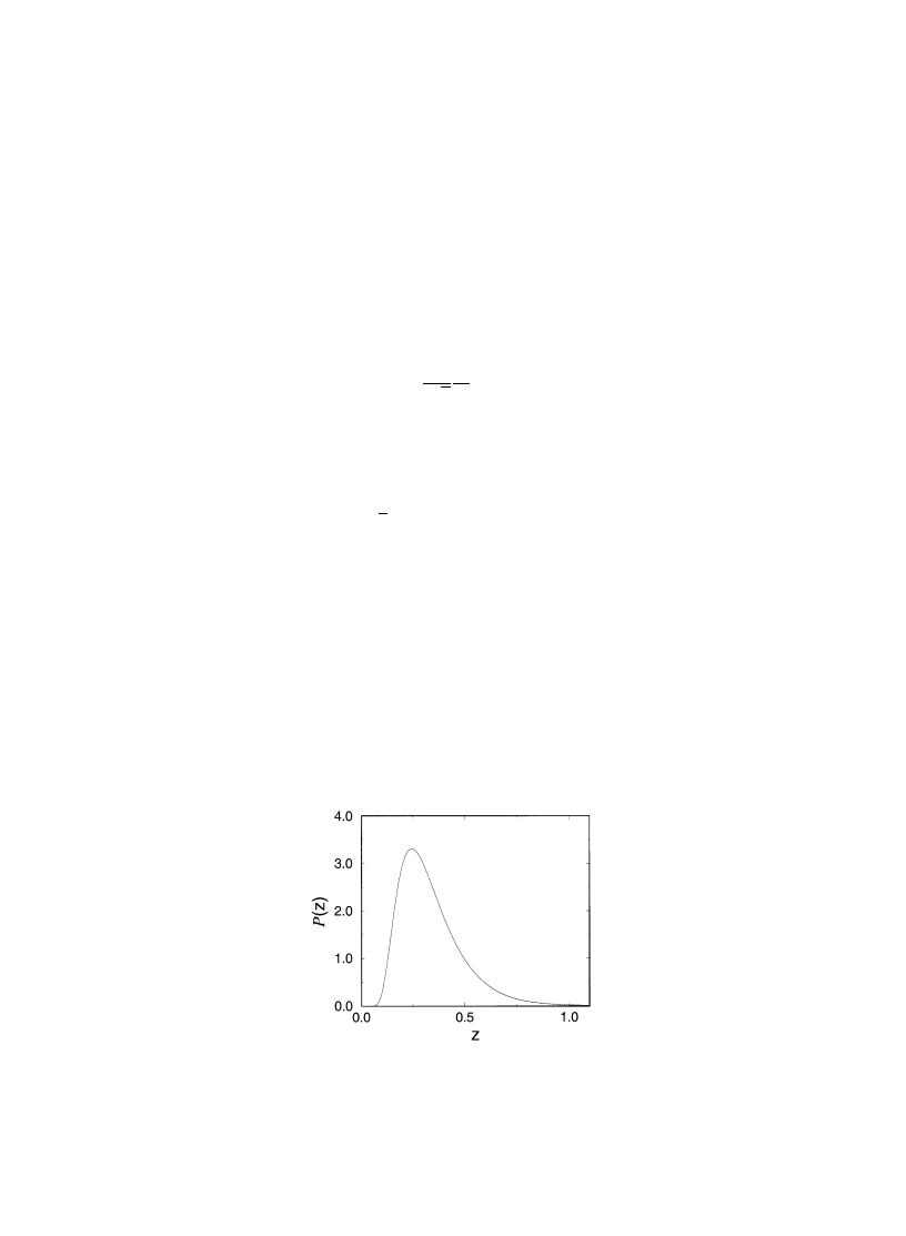
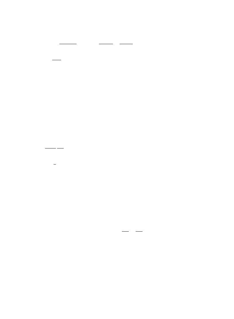
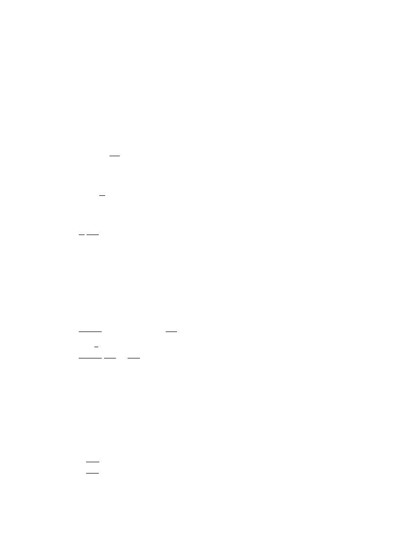
Fig. 1. Distribution function P(z) of the normalized (dimensionless) inverse participation ratio z"[

b2/(b#2)]plDA2P2

in a long (¸<

m) quasi-1D sample. The average value is SzT"1/3. From [18].

as in the region of very large amplitude in the metallic sample, Eq. (3.44). On this basis, it was
conjectured in [18] that the asymptotic behavior (3.44) is controlled by the probability to have
a quasi-localized eigenstate with an e!ective spatial extent much less than

m (`anomalously

localized state

a). This conjecture was proven rigorously in [36] where the shape of the anomalously

localized state (ALS) responsible for the large-u asymptotics was calculated via the transfer-matrix
method. We will discuss this in Section 4 devoted to ALS and to asymptotics of di!erent
distribution functions.

Distribution of the inverse participation ratio (IPR) is also found to have a simple form in the

limit ¸<

m [22,25]:

P(z)"2

k/1

p2zk4!3k2)e~p

~3@2

k/1

2e~k

(3.48)

where z"

plDA2P2 in the unitary case and z"(plDA2/3)P2 in the orthogonal case. (The second

line in (3.48) can be obtained from the "rst one by using the Poisson summation formula.)
Therefore, the spatial extent of a localized eigenfunction measured by IPR #uctuates strongly (of
order of 100%) from one eigenfunction to another. More precisely, the ratio of the r.m.s. deviation
of IPR to its mean value is equal to 1/

J5 according to Eq. (3.48). The

"rst form of Eq. (3.48) is more

suitable for extracting the asymptotic behavior of P(z) at z<1, whereas the second line gives us the
leading behavior of P(z) at small z;1:

P(z)"

p4ze~p

z<1 ,

p~1@2z~7@2e~1@z, z;1 .

(3.49)

Therefore, the probability to have atypically large or atypically small IPR is exponentially
suppressed. The function P(z) is presented in Fig. 1.

The above #uctuations of IPR are due to #uctuations in the

`central bumpa of a localized

eigenfunction. They should be distinguished from the #uctuations in the rate of exponential decay
of eigenfunctions (Lyapunov exponent). The latter can be extracted from another important

A.D. Mirlin / Physics Reports 326 (2000) 259}382

282

physical quantity } the distribution function P(v), where

v"(2

plDA2)2Dt2a(r1)t2a(r2)D

is the product of the eigenfunction intensity in the two points close to the opposite edges of the
sample r1P0, r2P¸. The result is [23,18]

P(!ln v)"F[!(

b ln v)/2X]

2(2

pX/b)1@2

exp

(2X/

b#ln v)2

U(u)"u

C2[(3!u)/2]

C(u)

O(u)"

C2[(1!u)/2]

pC(u)

(3.50)

Therefore, ln v is asymptotically distributed according to the Gaussian law with the mean value
S!ln vT"(2b)X"¸/bplAD and the variance var(!ln v)"2S!ln vT. The same log-normal
distribution is found for the conductance and for transmission coe$cients of a quasi-1D sample
from the Dorokhov}Mello}Pereyra}Kumar formalism [116,74] (see end of Section 6.2).

Note that the formula (3.50) is valid in the region of v;1 (i.e. negative ln v) only, which contains

almost all normalization of the distribution function. In the region of still higher values of v
the log-normal form of P(v) changes into the much faster stretched-exponential fall-o!
J

exp

M!2J2bv1@4N, as can be easily found from the exact solution given in [23,18]. The decay

rate of all the moments

SvkT, k52, is four times less than S!ln vT and does not depend on k:

SvkTJe~X@2b. This is because the moments SvkT, k52, are determined by the probability to

"nd

`anomalously delocalized statea with v&1.

3.3. Arbitrary dimensionality: metallic regime

3.3.1. Distribution of eigenfunction amplitudes

In the case of arbitrary dimensionality d, deviations from the RMT distribution P(y) for not too

large y can be calculated [24,25] via the method described in Section 2. Applying this method to the
moments (3.6), one gets

SDt(r)D2qT"

1
2

iq(q!1)#2

(U) ,

(3.51)

SDt(r)D2qT"

(2q!1)!!

[1#

iq(q!1)#2] (O) ,

(3.52)

where

i"P(r, r). Correspondingly, the correction to the distribution function reads

P(y)"e

i
2

(2!4y#y

2)#2

(U) ,

(3.53)

P(y)"

~y@2

J2py

3
2

3y#

(O) .

(3.54)

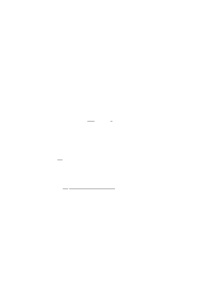
Deviations of the eigenfunction distribution function P(y) from its RMT form are illustrated for the
orthogonal symmetry case in Fig. 2. Numerical studies of the statistics of eigenfunction amplitudes

283

A.D. Mirlin / Physics Reports 326 (2000) 259}382

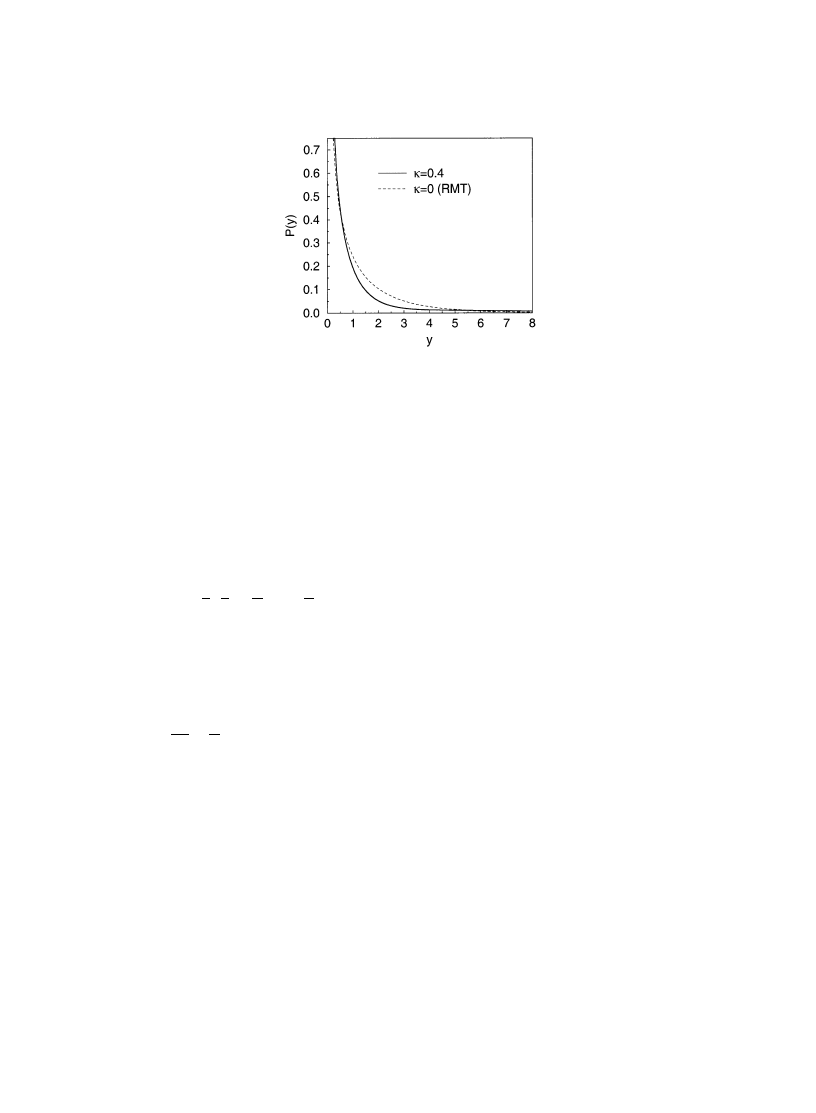
Fig. 2. Distribution P(y) of the normalized eigenfunction intensities y"<

Dt2(r)D in the orthogonal symmetry case. The

dotted line shows the RMT result, Eq. (3.2), while the full line corresponds to Eq. (3.54) with

i"0.4.

in weak localization regime have been performed in Ref. [117] for the 2D and in Ref. [118] for the
3D case. The found deviations from RMT are well described by the above theoretical results.
Experimentally, statistical properties of the eigenfunction intensity have been studied for micro-
waves in a disordered cavity [15]. For a weak disorder the found deviations are in good agreement
with (3.54) as well.

In the quasi-one-dimensional case (with hard wall boundary conditions in the longitudinal

direction), the one-di!uson loop

P(r, r) is equal to

i,P(r, r)"

2
g

1
3

04x4¸ ,

(3.55)

so that Eqs. (3.53) and (3.54) agree with results (3.40) and (3.41) obtained from the exact solution.
For the periodic boundary conditions in the longitudinal direction (a ring) we have

i"1/6g. In the

case of 2D geometry,

P(r, r)"

(3.56)

with g"2

plD. Finally, in the 3D case the sum over the momenta P(r, r)"(pl<)~1

(Dq

2)~1

diverges linearly at large q. The di!usion approximation is valid up to q&l

~1; the corresponding

cut-o! gives

P(r, r)&1/2plDl"g~1(¸/l). This divergency indicates that more accurate evaluation

P(r, r) requires taking into account also the contribution of the ballistic region (q'l~1)

which depends on microscopic details of the random potential. We will return to this question in
Section 3.3.4.

The formulas (3.53) and (3.54) are valid in the region of not too large amplitudes, where the

perturbative correction is smaller than the RMT term, i.e. at y;

i~1@2. In the region of large

amplitudes, y'

i~1@2 the distribution function was found by Fal

'ko and Efetov [32,33], who

applied to Eqs. (3.12) and (3.14) the saddle-point method suggested by Muzykantskii and Khmel-
nitskii [29]. We relegate the discussion of the method to Section 4 and only present the results here:

A.D. Mirlin / Physics Reports 326 (2000) 259}382

284

P(y)Kexp

b
2

iy2

]

(U)

J2py

(O)

i~1@2[y[i~1 ,

(3.57)

P(y)&exp

d(iy)

Zi~1 .

(3.58)

Again, as in the quasi-one-dimensional case, there is an intermediate range where a correction in
the exponent is large compared to unity, but small compared to the leading RMT term [Eq. (3.57)]
and a far asymptotic region (3.58), where the decay of P(y) is much slower than in RMT. In the next
section we will discuss the structure of anomalously localized eigenstates, which are responsible for
the asymptotic behavior (3.44), (3.58).

3.3.2. 2D: Weak multifractality of eigenfunctions

Since d"2 is the lower critical dimension for the Anderson localization problem, metallic 2D

samples (with g<1) share many common properties with systems at the critical point of the
metal}insulator transition. Although the localization length

m in 2D is not in

"nite (as for truly

critical systems), it is exponentially large, and the criticality takes place in the very broad range of
the system size ¸;

3.3.2.1. Multifractality: basic dexnitions.

The criticality of eigenfunctions shows up via their

multifractality. Multifractal structures "rst introduced by Mandelbrot [119] are characterized by
an in"nite set of critical exponents describing the scaling of the moments of a distribution of some
quantity. Since then, this feature has been observed in various objects, such as the energy
dissipating set in turbulence [120}122], strange attractors in chaotic dynamical systems [123}126],
and the growth probability distribution in di!usion-limited aggregation [127}129]; see Ref. [130]
for a review.

The fact that an eigenfunction at the mobility edge has the multifractal structure was noticed for

the "rst time in [51], though the underlying renormalization group calculations were done by
Wegner several years earlier [50]. For this problem, the probability distribution is just the
eigenfunction intensity

Dt2(r)D and the corresponding moments are the inverse participation ratios,

Pq"

drDt2q(r)D .

(3.59)

The multifractality is characterized by the anomalous scaling of Pq with the system size ¸,

PqJ¸~D

(q~1),¸~q(q) ,

(3.60)

with Dq di!erent from the spatial dimensionality d and dependent on q. Equivalently, the

eigenfunctions are characterized by the singularity spectrum f (

a) describing the measure ¸f(a) of

the set of those points r where the eigenfunction takes the value

Dt2(r)DJ¸~a. The two sets of

exponents

q(q) and f (a) are related via the Legendre transformation,

q(q)"qa!f (a), f @(a)"q, q@(q)"a .

(3.61)

For a recent review on multifractality of critical eigenfunctions the reader is referred to [55,131].

285

A.D. Mirlin / Physics Reports 326 (2000) 259}382

3.3.2.2. Multifractality in 2D. We note "rst that the formulas (3.51) and (3.52) for the IPRs with
q

[i~1@2 can be rewritten in the 2D case (with (3.56) taken into account) as

SPqT

RMT

(1@bpg)q(q~1)

(3.62)

where P

RMT

is the RMT value of Pq equal to q!¸~2(q~1) for GUE and (2q!1)!!¸~2(q~1) for GOE.

We see that (3.62) has precisely the form (3.60) with

Dq"2!(q/bpg) .

(3.63)

As was found in [32,33], the eigenfunction amplitude distribution (3.57), (3.58) leads to the same
result (3.63) for all q;2

bpg. Since deviation of Dq from the normal dimension 2 is proportional to

the small parameter 1/

pg, it can be termed `weak multifractalitya (in analogy with weak localiza-

tion). The result (3.63) was in fact obtained for the "rst time by Wegner [50] via the renormalization
group calculations.

The limits of validity of Eq. (3.63) are not unambiguous and should be commented here. The

singularity spectrum f (

a) corresponding to (3.63) has the form

f (

a)"2!

bpg

(3.64)

so that f (

aB"0) for

aB"2

bpg)1@2

(3.65)

a lies outside the interval (a~,a`), the corresponding f(a)(0, which means that the most likely

the singularity

a will not be found for a given eigenfunction. However, if one considers the average

SPqT over a su$ciently large ensemble of eigenfunctions (corresponding to di!erent realizations of

disorder), a negative value of f (

a) makes sense (see a related discussion in [132,133]). This is the

de"nition which was assumed in [32,33] where Eq. (3.63) was obtained for all positive q;2

bpg.

In contrast, if one studies a typical value of Pq, the regions a'a` and a(a~ will not

contribute. In this case, Eq. (3.63) is valid only within the interval q~4q4q` with

qB"$(2bpg)1@2; outside this region one "nds [134,135]

q(q),Dq(q!1)"

a~, q'q` ,

a`, q(q~ .

(3.66)

Therefore, within this de"nition the multifractal dimensions Dq saturate at the values a` and

a~ for qP#R and qP!R, respectively. This is in agreement with results of numerical

simulations [52}56].

3.3.3. Correlations of eigenfunction amplitudes and yuctuations of the inverse participation ratio

In this subsection, we study correlations of eigenfunctions in the regime of a good conductor

[25}27,136,137]. The correlation function of amplitudes of one and the same eigenfunction with

A.D. Mirlin / Physics Reports 326 (2000) 259}382

286

energy E can be formally de"ned as follows:

a(r1,r2,E)"SDtk(r1)tk(r2)D2TE,D

Dtk(r1)tk(r2)D2d(E!ek)

(3.67)

An analogous correlation function for two di!erent eigenfunctions is de"ned as

p(r1,r2,E,u)"SDtk(r1)tl(r2)D2TE,u

D2R~1(u)

kEl

Dtk(r1)tl(r2)D2d(E!ek)d(E#u!el)

(3.68)

where R(

u) is the two-level correlation function (2.1). To evaluate a(r1,r2,E) and p(r1,r2,E,u), we

employ an identity

p2[D~1a(r1,r2,E)d(u)#D~2RI(u)p(r1,r2,E,u)]

Re[

SGR(r1,r1,E)GA(r2,r2,E#u)!GR(r1,r1,E)GR(r2,r2,E#u)T] ,

(3.69)

where G

R,A(r, r@, E) are retarded and advanced Green

's functions and R

I (u) is the non-singular part

of the level-level correlation function: R(

u)"RI(u)#d(u/D). A natural question, which arises at

this point, is whether the r.h.s. of Eq. (3.69) cannot be simply found within the di!uson-Cooperon
perturbation theory [9]. Such a calculation would, however, be justi"ed only for

u<D (more

precisely, one has to introduce an imaginary part of frequency:

uPu#iC, and require that

C<D). Therefore, it would only allow to

"nd a smooth in

u part of p(r1,r2,E,u) for u<D.

Evaluation of

a(r1,r2,E), as well as of p(r1,r2,E,u) at u&D, cannot be done within such

a calculation. For this reason the non-perturbative supersymmetry approach is to be used.

The r.h.s. of Eq. (3.69) can be expressed in terms of the supermatrix

p-model, yielding:

p2[D~1a(r1,r2,E)d(u)#D~2p(r1,r2,E,u)RI(u)]

(

pl)2[1!ReSQ11

(r1)Q22

(r2)TS!kd(r1!r2)ReSQ12

(r1)Q21

(r1)TS] ,

(3.70)

where

TS denotes the averaging with the sigma-model action and kd(r)"(pl)~2SImGR(r)T2 is

a short-range function explicitly given by

kd(r)"exp(!r/l)

20(pFr),

2D ,

(pFr)~2sin2pFr, 3D .

(3.71)

We consider the unitary ensemble "rst; results for the orthogonal symmetry will be presented in the
end. Evaluating the

p-model correlation functions in the r.h.s. of Eq. (3.70) and separating the result

into the singular the singular (proportional to

d(u)) and regular at u"0 parts, one can obtain the

correlation functions

a(r1,r2,E) and p(r1,r2,E,u). The two-level correlation function R(u) entering

Eq. (3.70) was studied in Section 2. We employ again the method of [10] described in Section 2 to
calculate the sigma-model correlation functions

SQ11

(r1)Q22

(r2)TS and SQ12

(r1)Q21

(r2)TS for

relatively low frequencies

u;Ec. First, we restrict ourselves to the terms of order g~1. Then, the

result for the "rst correlation function reads as

SQ11

(r1)Q22

(r2)TS"!1!2i

exp(i

ps)sin ps

(

ps)2

P(r1,r2) ,

(3.72)

287

A.D. Mirlin / Physics Reports 326 (2000) 259}382

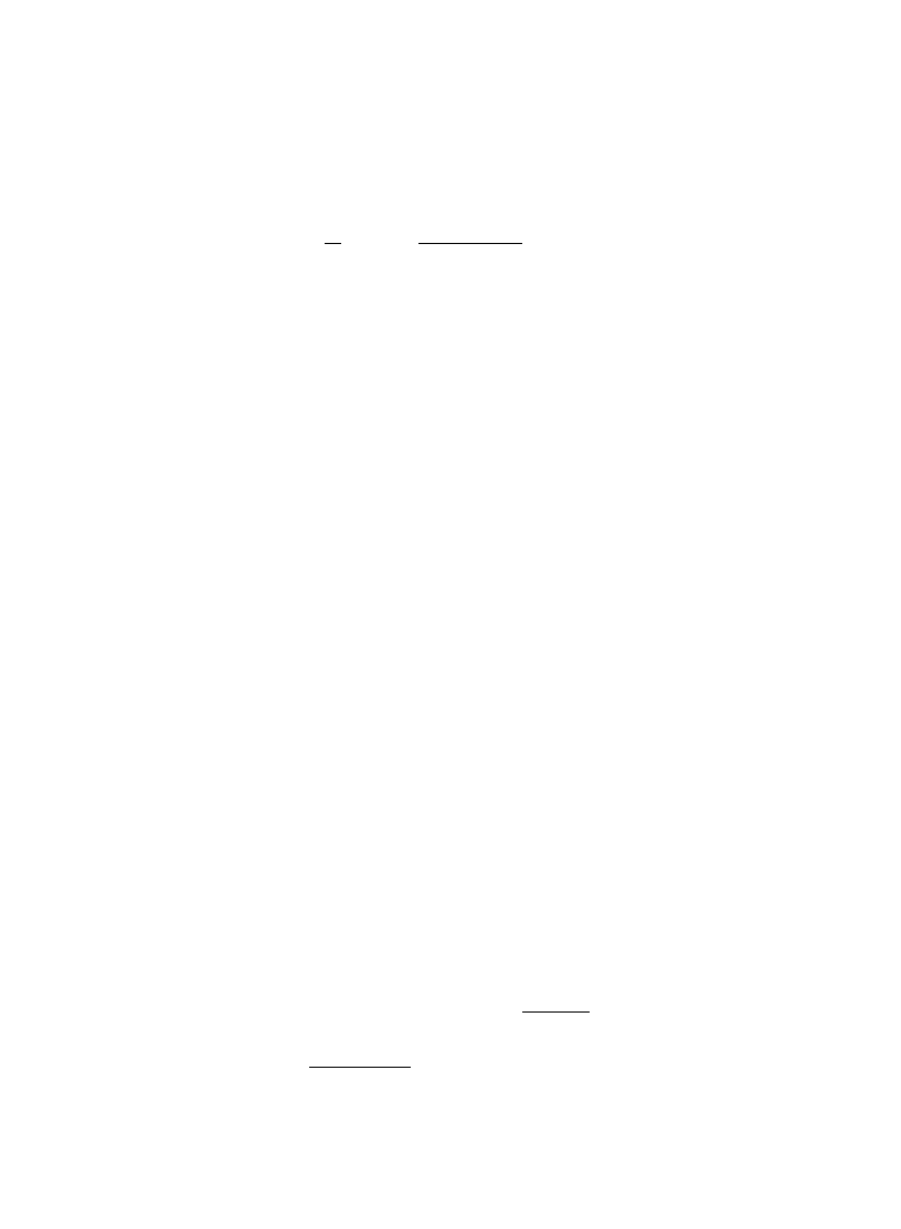
where s"

u/D#i0. The

"rst

two terms in Eq. (3.72) represent the result of the zero-mode

approximation; the last term is the correction of order g

~1. An analogous calculation for the

second correlator yields:

SQ12

(r1)Q21

(r2)TS"!2

1#i

exp(i

ps) sin ps

(

ps)2

P(r1,r2)

(3.73)

Now, separating regular and singular parts in r.h.s. of Eq. (3.70), we obtain the following result [27]
for the autocorrelations of the same eigenfunction:

2SDtk(r1)tk(r2)D2TE!1"kd(r)[1#P(r1,r1)]#P(r1,r2) ,

(3.74)

and for the correlation of amplitudes of two di!erent eigenfunctions

2SDtk(r1)tl(r2)D2TE,u!1"kd(r)P(r1,r1), kOl.

(3.75)

In particular, for r1"r2 we have

2SDtk(r)tlr)D2TE,u!1"dkl#(1#dkl)P(r,r) .

(3.76)

Note that the result (3.74) for r1"r2 is the inverse participation ratio calculated above (Section

3.3.1); on the other hand, neglecting the terms with the di!usion propagator (i.e. making the
zero-mode approximation), we reproduce the result of Refs. [110}112].

Eqs. (3.75) and (3.76) show that the correlations between di!erent eigenfunctions are relatively

small in the weak disorder regime. Indeed, they are proportional to the small parameter

P(r, r). The

correlations are enhanced by disorder; when the system approaches the strong localization regime,
the relative magnitude of correlations,

P(r, r) ceases to be small. The correlations near the

Anderson localization transition will be discussed in Section 5.

Another correlation function, generally used for the calculation of the linear response of the

system,

c(r1,r2,E,u)"StHk(r1)tl(r1)tk(r2)tHl(r2)TE,u

D2R~1(u)

kEl

tHk(r1)tl(r1)tk(r2)tHl(r2)d(E!ek)d(E#u!el)

(3.77)

can be calculated in a similar way. The result reads

2StHk(r1)tl(r1)tk(r2)tHl(r2)TE,u"kd(r)#P(r1,r2), kOl.

(3.78)

As is seen from Eqs. (3.74), (3.75) and (3.78), in the 1/g order the correlation functions

a(r1,r2,E)

and

c(r1,r2,E,u) survive for the large separation between the points, r<l, while p(r1,r2,E,u)

decays exponentially for the distances larger than the mean free path l. This is, however, an artifact
of the g

~1 approximation, and the investigation of the corresponding tails requires the extension of

the above calculation to the terms proportional to g

~2. The correlator SQ11

(r1)Q22

(r2)TS gets the

following correction in the g

~2 order:

dSQ11

)

TS"!f1#2f4#exp(2ips)f3!2i

exp(2i

ps)

( f2!f3)

exp(2i

ps)!1

ps)2

( f1!4f2#3f3!2f4) ,

(3.79)

A.D. Mirlin / Physics Reports 326 (2000) 259}382

288

where we de"ned the functions

f1(r1,r2)"P2(r1, r2) ,

f2(r1,r2)"(2<)~1

dr[

P2(r, r1)#P2(r,r2)] ,

f3"<~2

dr dr

@ P2(r, r@) ,

f4(r1,r2)"<~1

P(r, r1)P(r,r2) .

(3.80)

Consequently, we obtain the following results for the correlations of di!erent (kOl) eigenfunctions
at r'l:

2SDtk(r1)tl(r2)D2TE,u!1"

1
2

( f1!f3!2f4)

2( f2!f3)

sin

2 ps

(

ps)2

sin 2

sin

2 ps

(

ps)2

(3.81)

As it should be expected, the double integral over the both coordinates of this correlation function
is equal to zero. This property is just the normalization condition and should hold in arbitrary
order of expansion in g

~1.

The quantities f2, f3, and f4 are proportional to g~2, with some (geometry-dependent) prefactors

of order unity. On the other hand, f1 in 2D and 3D geometry depends essentially on the distance

Dr1!r2D. In particular, for l;r;¸

f1(r1,r2)"P2(r1, r2)+

(

pg)2

2D ,

p2lDr)2

3D .

Thus, for l(r;¸, the contributions proportional to f1 dominate in Eq. (3.81), yielding

2SDtk(r1)tl(r2)D2TE,u!1"12P2(r1,r2), kOl .

(3.82)

On the other hand, for the case of the quasi-1D geometry (as well as in 2D and 3D for r&¸), all
quantities f1, f2, f3, and f4 are of order of 1/g2. Thus, the correlator p(r1,r2, E, u) acquires

a non-trivial (oscillatory) frequency dependence on a scale

u&D described by the second term in

the r.h.s. of Eq. (3.81). In particular, in the quasi-1D case the function f2!f3 determining the

spatial dependence of this term has the form

f2!f3"!

(3.83)

where B4(x)"x4!2x3#x2!1/30 is the Bernoulli polynomial.

289

A.D. Mirlin / Physics Reports 326 (2000) 259}382

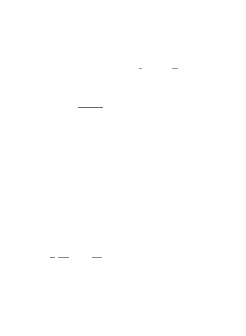
Let us remind the reader that the above derivation is valid for

u;Ec. In the range uZEc the

p-model correlation functions entering Eqs. (3.70) can be calculated by means of the perturbation
theory [9], yielding

2SDtk(r1)tl(r2)D2TE,u"1#Re

kd(r)Pu(r1, r2)#

1
2

P2u(r1,r2)!

dr dr

@P2u(r,r@)

2StHk(r1)tl(r1)tk(r2)tHl(r2)TE,u"kd(r)#RePu(r1,r2) ,

(3.84)

where

Pu(r1,r2) is the "nite-frequency di!usion propagator

Pu(r1,r2)"(pl)~1+

/q(r1)/q(r2)

2!iu

(3.85)

and the summation in Eq. (3.85) now includes q"0. As was mentioned, the perturbation theory
should give correctly the non-oscillatory (in

u) part of the correlation functions at u<D. Indeed, it

can be checked that Eqs. (3.84) match the results (3.75) and (3.78) of the non-perturbative
calculation in this regime. Furthermore, in the 1/g order [which means keeping only linear in
Pu terms in (3.84) and neglecting !iu in denominator of Eq. (3.85)]. Eqs. (3.84) and (3.85)

reproduce the exact results (3.75) and (3.78) even at small frequencies

u&D. We stress, however,

that the perturbative calculation is not justi"ed in this region and only the supersymmetry method
provides a rigorous derivation of these results.

Generalization to a system with unbroken time reversal symmetry (orthogonal ensemble) is

straightforward [138]; in the 1/g-order Eqs. (3.74), (3.75), and (3.78) are modi"ed as follows:

2SDtk(r1)tk(r2)D2TE"[1#2kd(r)][1#2P(r1,r2)] ,

(3.86)

2SDtk(r1)tl(r2)D2TE,u!1"2kd(r)P(r1,r2) ,

(3.87)

2StHk(r1)tl(r1)tk(r2)tHl(r2)TE,u"kd(r)#[1#kd(r)]P(r1,r2), kOl .

(3.88)

3.3.3.1. IPR yuctuations. Using the supersymmetry method, one can calculate also higher-order
correlation functions of the eigenfunction amplitudes. In particular, the correlation function
SDt4k(r1)DDt4k(r2)DTE determines #uctuations of the inverse participation ratio (IPR) P2":drDt4(r)D.

Details of the corresponding calculation can be found in Ref. [25]; the result for the relative
variance of IPR,

d(P2)"var(P2)/SP2T2 reads

d(P2)"

dr dr

P2(r, r@)"

32ad

b2g2

(3.89)

with a numerical coe$cient ad de"ned in Section 2 (see Eqs. (2.25) and (2.26)). The #uctuations

(3.89) have the same relative magnitude (&1/g) as the famous universal conductance #uctuations.
Note also that extrapolating Eq. (3.89) to the Anderson transition point, where g&1, we "nd
d(P2)&1, so that the magnitude of IPR #uctuations is of the order of its mean value (which is, in

turn, much larger than in the metallic regime; see Section 5).

A.D. Mirlin / Physics Reports 326 (2000) 259}382

290

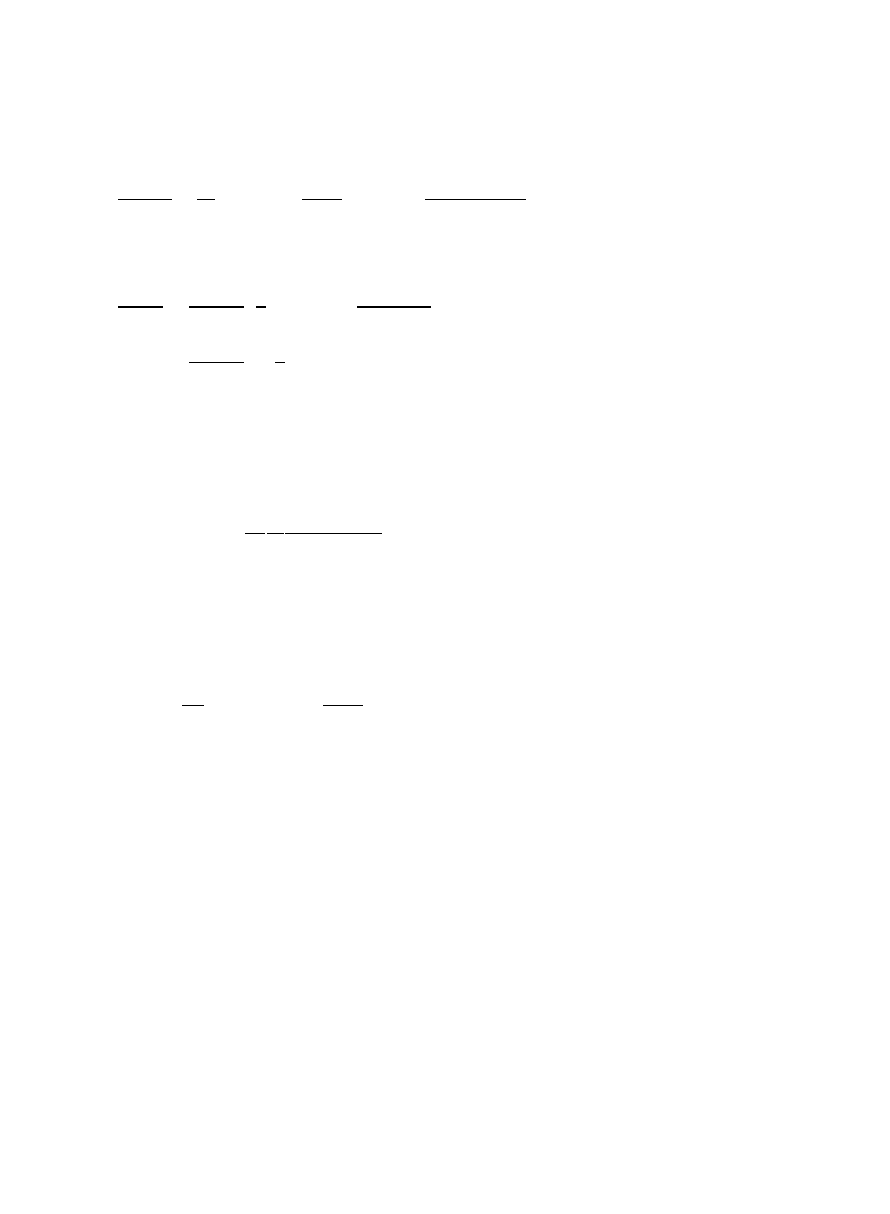
Eq. (3.89) can be generalized onto higher IPRs Pq with q'2,

var(Pq)

SPqT2

2(q!1)2

dr dr

P2(r, r@)"

2(q!1)2ad

b2g2

(3.90)

so that the relative magnitude of #uctuations of Pq is &q(q!1)/g. Furthermore, the higher

irreducible moments (cumulants)

|Pnq}, n"2,3,2, have the form

|Pnq}

SPqTn

(n!1)!

q(q!1)

dr12drn

P(r1,r2)2P(rn,r1)

(n!1)!

2
b

q(q!1)

(3.91)

where

P is the integral operator with the kernel P(r, r@)/<. This is valid provided q2n;2bpg.

Prigodin and Altshuler [137] obtained Eq. (3.91) starting from the assumption that the eigen-
function statistics is described by the Liouville theory. According to (3.91), the distribution
function P(Pq) of the IPR Pq (with q2/bpg;1) decays exponentially in the region

q(q!1)/g;Pq/SPqT!1;1,

P(Pq)&exp

Pq/SPqT!1

q(q!1)

(3.92)

where

e1 is the lowest non-zero eigenvalue of the di!usion operator !D+2.

The perturbative calculations show that the cumulants of the IPRs are correctly reproduced (in

the leading order in 1/g) if one assumes [137] that the statistics of the eigenfunction envelopes
Dt2(r)D4.005)"eh(

) is governed by the Liouville theory (see, e.g. [139,140]) de

"ned by the functional

integral

h d

h!1

exp

bplD

dr(+h)2

2 .

(3.93)

We will return to this issue in Section 4 where the asymptotics of the IPR distribution function will
be discussed. We will see that these

`tailsa governed by rare realizations of disorder are described

by saddle-point solutions which can be also obtained from the Liouville theory description (3.93).
The multifractal dimensions (3.63) can be found from the Liouville theory as well [139,140]. It
should be stressed, however, that this agreement between the supermatrix

p-model governing the

eigenfunctions statistics and the Liouville theory is not exact, but only holds in the leading order
in 1/g.

Let us note that the correlations of eigenfunction amplitudes determine also #uctuations of

matrix elements of an operator of some (say, Coulomb) interaction computed on eigenfunctions
tk of the one-particle Hamiltonian in a random potential. Such a problem naturally arises, when

one wishes to study the e!ect of interaction onto statistical properties of excitations in a mesoscopic
sample (see Section 9).

3.3.4. Ballistic ewects
3.3.4.1. Ballistic systems. The above consideration can be generalized to a ballistic chaotic system,
by applying a recently developed ballistic generalization of the

p-model [75

}77]. The results are

291

A.D. Mirlin / Physics Reports 326 (2000) 259}382

then expressed [78] in terms of the (averaged over the direction of velocity) kernel g(r1,n1; r2, n2) of

the Liouville operator K

K "vFn+ governing the classical dynamics in the system,

PB(r1,r2)"

dn1 dn2 g(r1, n1;r2, n2) ,

K g(r1,n1;r2,n2)"(pl)~1[d(r1!r2)d(n1!n2)!<~1] .

(3.94)

Here n is a unit vector determining the direction of momentum, and normalization

:dn"1 is used.

Equivalently, the function

PB(r1,r2) can be de"ned as

PB(r1,r2)"

dn1 g8(r1,n1, t;r2) ,

(3.95)

where g

8 is determined by the evolution equation

vFn1+1

8 (r1,n1,t;r2)"0, t'0

(3.96)

with the boundary condition

8 Dt/0"(pl)~1[d(r1!r2)!<~1] .

(3.97)

Eq. (3.94) is a natural

`ballistica counterpart of Eq. (2.22). Note, however, that PB(r1, r2) contains

a contribution

P(0)

(r1, r2) of the straight line motion from r2 to r

(equal to 1/(

ppFDr1!r2D) in 2D

and to 1/2(pFDr1!r2D)2 in 3D), which is nothing else but the smoothed version of the function

kd(Dr1!r2D). For this reason, P(r1, r2) in Eqs. (3.86)}(3.88) should be replaced in the ballistic case

P(r1,r2)"PB(r1,r2)!P(0)B(r1,r2). At large distances Dr1!r2D<jF the (smoothed) correlation

function takes in the leading approximation the form

2a(r1,r2,E)"1#

PB(r1,r2) .

(3.98)

A formula for the variance of matrix elements closely related to Eq. (3.98) was obtained in the
semiclassical approach in Ref. [141]. In a recent paper [142] a similar generalization of the Berry
formula for

StHk(r1)tk(r2)T was proposed.

Eq. (3.98) shows that correlations in eigenfunction amplitudes in remote points are determined

by the classical dynamics in the system. It is closely related to the phenomenon of scarring of
eigenfunctions by the classical orbits [143,144]. Indeed, if r1 and r2 belong to a short periodic orbit,

the function

PB(r1,r2) is positive, so that the amplitudes Dtk(r1)D2 and Dtk(r2)D2 are positively

correlated. This is a re#ection of the

`scarsa associated with this periodic orbits and a quantitative

characterization of their strength in the coordinate space. Note that this e!ect gets smaller with
increasing energy E of eigenfunctions. Indeed, for a strongly chaotic system and for

Dr1!r2D&¸ (¸

being the system size), we have in the 2D case

PB(r1,r2)&jF/¸, so that the magnitude of

correlations decreases as E

~1@2. The function PB(r1,r2) was explicitly calculated in Ref. [78] for

a circular billiard with di!use surface scattering (see Section 8).

3.3.4.2. Ballistic ewects in diwusive systems. We return now to the question of deviations of the
eigenfunction amplitude distribution from the RMT in a di!usive 3D sample. As was shown in

A.D. Mirlin / Physics Reports 326 (2000) 259}382

292

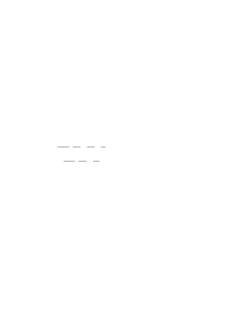
Section 3.3.1, such deviations are controlled by the parameter

i"P(r, r), see Eqs. (3.53)

}(3.56). The

physical meaning of the parameter

i is the time-integrated return probability, see Eq. (3.95)

generalizing de"nition of

P(r1,r2) to the ballistic case. The contribution to this return probability

from the times larger than the momentum relaxation time, t'

q, is given by

P$*&&(r, r)"(pl<)~1 +

[

1@l

(Dq

2)~1 .

The sum over the momenta diverges on the ultraviolet bound in d52, so that the cut-o! at q&1/l
is required. This results in Eq. (3.56) in 2D and in

P$*&&(r, r)&1/(kFl)2 in the 3D case. There exists,

however, an additional, ballistic, contribution to

P(r, r), which comes from the times t shorter than

the mean free time

q. Diagrammatically, it is determined by the

"rst term of the di!uson ladder

contributing to

P(r, r) (that with one impurity line), i.e. by the probability to hit an impurity and to

be rejected back after a time t;

q. Contrary to the di

!usive contribution, which has a universal

form and is determined by the value of the di!usion constant D only, the ballistic one is strongly
dependent on the microscopic structure of the disorder. In particular, in the case of the white-noise
disorder we "nd

P"!--(r, r)"

plv2Fq

(dq)

2D ,

lv2Fq

(dq)

kFl

3D .

(3.99)

Note that the integrals over the momenta are again divergent at large q } precisely in the same way
as in the di!usive region, but with di!erent numerical coe$cients } and are now cut-o! at q&kF.

The total return probability is given by the sum of the short-scale (ballistic) and long-scale

(di!usive) contributions. It is important to notice, however, that the single-scattering contribution
(3.99) should be divided by 2 in the orthogonal symmetry case, because the corresponding
trajectory is identical to its time reversal. Thus,

i"P$*&&(r, r)#P"!--(r, r) for b"2 and

i"P$*&&(r, r)#(1/2)P"!--(r, r) for b"1. We see that for the white-noise random potential in 3D the
return probability is dominated by the ballistic contribution, yielding

i&1/kFl. In the 2D case,

taking into account of the ballistic contribution modi"es only the argument of the logarithm
in (3.56). Furthermore, even in the quasi-1D geometry the non-universal short-scale e!ects
can be important. Indeed, if we consider a 3D sample of the quasi-1D geometry (¸x,¸y;¸z),

the di!usion contribution will be given by Eq. (3.55),

P$*&&(r, r)&1/g, while the ballistic one

will be

P"!--(r, r)&1/kFl. Therefore, the di!usion contribution is dominant only provided

g;kFl.

On the other hand, let us consider the opposite case of a smooth random potential with

correlation length d<

jF. Then the scattering is of small-angle nature and the probability for

a particle to return back in a time t;

q is exponentially small, so that P"!--(r, r) can be neglected.

Therefore, the return probability

i in Eqs. (3.51)

}(3.54) is correctly given by the di!usion contribu-

tion, see Eq. (3.56) for 2D and the estimate below it for 3D. Thus the corrections to the

`bodya of

the distribution function are properly given by the

p-model in this case.

293

A.D. Mirlin / Physics Reports 326 (2000) 259}382

4. Asymptotic behavior of distribution functions and anomalously localized states

In this section, we discuss asymptotics of distribution functions of various quantities characteriz-

ing wave functions in a disordered system. Asymptotic behavior of these distribution functions is
determined by rare realizations of the disorder producing the states, which show much stronger
localization features than typical states in the system. We call such states

`anomalously localized

states

a (ALS).

It was found by Altshuler, Kravtsov and Lerner (AKL) [28] that distribution functions of conduc-

tance, density of states, local density of states, and relaxation times have slowly decaying logarithmically
normal (LN) asymptotics at large values of the arguments. These results were obtained within the
renormalization group treatment of the

p-model. The validity of this RG approach is restricted to 2D

and 2#

e-dimensional systems, with e;1. On the other hand, the conductance, LDOS and relaxation

times #uctuations in strictly 1D disordered chains, where all states are strongly localized, were
studied with the use of Berezinski and Abrikosov}Ryzhkin techniques [113,145}148]. The corre-
sponding distributions were found to be of the LN form, too. It was conjectured on the basis of this
similarity [28,113,149] that even in a metallic sample there is a "nite probability to "nd

`almost

localized

a eigenstates, and that these states govern the slow asymptotic decay of the distribution

functions. Similar conclusion [25] is implied by the exact results for the statistics of the eigenfunc-
tion amplitude in the quasi-one-dimensional case, which shows the identical asymptotic behavior
in the localized and metallic regimes, see Section 3, Eqs. (3.44) and (3.47).

A new boost to the activity in this direction was given by the paper of Muzykantskii and

Khmelnitskii [29], who proposed to use the saddle-point method for the supersymmetric

p-model

in order to calculate the long-time dispersion of the average conductance G(t). Their idea was to
reproduce the AKL result by means of a more direct calculation. However, they found a di!erent,
power-law decay of G(t) in an intermediate range of times t in 2D. As was shown by the author [30]
(and then reproduced in [31] within the ballistic

p-model approach), the far asymptotic behavior is

of log-normal form and is thus in agreement with AKL. The saddle-point method of Muzykantskii
and Khmelnitskii allowed also to study the asymptotic behavior of distribution functions of other
quantities: relaxation times [29}31], eigenfunction intensities [32,33], local density of states [34],
inverse participation ratio [35,36], level curvatures [37], etc. The form of the saddle-point solution
describes directly the spatial shape of the corresponding anomalously localized state [29,36].

We will consider the unitary symmetry (

b"2) throughout this section; in the general case, the

conductance g in the exponent of the distribution functions is replaced by (

b/2)g (we will sometimes

do it explicitly in the end of the calculation).

4.1. Long-time relaxation

In this subsection we study (mainly following Refs. [29,30]) the asymptotic (long-time) behavior

of the relaxation processes in an open disordered conductor. One possible formulation of the
problem is to consider the time dependence of the average conductance G(t) de"ned by the
non-local (in time) current}voltage relation

I(t)"

@ G(t!t@)<(t@) .

(4.1)

A.D. Mirlin / Physics Reports 326 (2000) 259}382

294

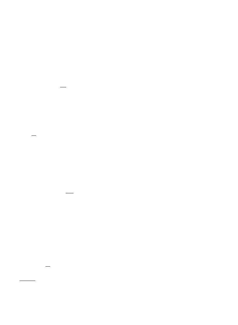
7 h1 is related to the eigenvalue j1 used in Section 3.1 as j1"coshh1.

Alternatively, one can study the decay law, i.e. the survival probability Ps(t) for a particle injected

into the sample at t"0 to be found there after a time t. Classically, Ps(t) decays according to the

exponential law, Ps(t)&e~t@t

, where t

is the lowest eigenvalue of the di!uson operator !D

with the proper boundary conditions. The time tD has the meaning of the time of di!usion through

the sample, and t

is the Thouless energy (see Section 2). The same exponential decay holds for the

conductance G(t), where it is induced by the weak-localization correction. The quantities of interest
can be expressed in the form of the

p-model correlation function

G(t), Ps(t)&

~*ut

DQ(r)A

MQNe~S*Q+ ,

(4.2)

where S[Q] is given by Eq. (3.7) with

gP!2iu. The preexponential factor AMQN depends on

speci"c formulation of the problem, but is not important for the leading exponential behavior
studied here.

Varying the exponent in Eq. (4.2) with respect to Q and

u, one gets the equations [29]

+(Q+Q)#iu[K, Q]"0 ,

(4.3)

dr Str(

KQ)"t .

(4.4)

[We assume unitary symmetry (

b"2); in the orthogonal symmetry case the calculation is

applicable with minor modi"cations and we will present the result in the end.] Note that in fact
u plays in (4.2) a role of the Lagrange multiplier corresponding to the condition (4.4).

Therefore, it remains

(i) to "nd a solution Qu of Eq. (4.3) (which will depend on u);

(ii) to substitute it into the self-consistency equation (4.4) and thus to "x

u as a function of t;

(iii) to substitute the found solution Qt into Eq. (4.2), which will yield

Ps(t)&exp

plD

Str

(

+Qt)2

(4.5)

Note that Eq. (4.3) is to be supplemented by the boundary conditions

D-%!$4"K

(4.6)

at the open part of the boundary, and

+nQD*/46-!503"0

(4.7)

at the insulating part of the boundary (if it exists);

+n denotes here the normal derivative.

It is not di$cult to show [29] the solution of Eq. (4.3) has in the standard parametrization the

only non-trivial variable } bosonic

`non-compact anglea7 04h1(R; all other coordinates being

equal to zero. As a result, Eq. (4.3) reduces to an equation for

h1(r) (we drop the subscript `1a below)

+2h#

sinh

h"0 ,

(4.8)

295

A.D. Mirlin / Physics Reports 326 (2000) 259}382

the self-consistency condition (4.4) takes the form

dr(cosh h!1)"t ,

(4.9)

and Eq. (4.5) can be rewritten as

ln Ps(t)"!

plD

dr(+h)2 .

(4.10)

For su$ciently small times,

h is small according to (4.9), so that Eqs. (4.8) and (4.9) can be linearized

+2h#2ch"0, 2c"iu/D ,

(4.11)

dr h2"t .

(4.12)

This yields

1@2

/1(r) ,

(4.13)

where

/1 is the eigenfunction of the Laplace operator corresponding to the lowest eigenvalue

c1"1/DtD. The survival probability (4.10) reduces thus to

ln Ps(t)"

plD

dr h+2h"!plDc1

dr h2"!t/tD ,

(4.14)

as expected. Eq. (4.14) is valid (up to relatively small corrections) as long as

h;1, i.e. for

D;1 (D"1/l< being the mean level spacing). To

"nd the behavior at t

ZD~1, as well corrections

at t(

D~1, one should consider the exact (non-linear) equation (4.8), solution of which depends on

the sample geometry.

4.1.1. Quasi-1D geometry

We consider a wire of a length ¸ and a cross-section A with open boundary conditions at both

edges,

h(!¸/2)"h(¸/2)"0. Eqs. (4.8) and (4.9) take the form

hA#2c sinh h"0 ,

(4.15)

L@2

~L@2

dx(cosh

h!1)"t/plA .

(4.16)

From the symmetry consideration

h(x)"h(!x) and h@(0)"0, so that it is su

$cient to consider the

region x'0. The solution of Eq. (4.15) reads

h(x)

Jc(cosh h0!cosh

)

(4.17)

A.D. Mirlin / Physics Reports 326 (2000) 259}382

296

where

h0 is determined by the condition h(¸/2)"0 yielding

¸"

Jc(cosh h0!cosh

)

(4.18)

In the large-t region (t

D<1) we will have h0<1, and Eqs. (4.17) and (4.18) can be simpli"ed to give

h(x)Kh0

(4.19)

h0Kln

h20

c¸2

(4.20)

Substituting this into condition (4.16) allows to relate

h0 to t,

*h0 .

(4.21)

Finally, substitution of Eqs. (4.19) and (4.21) into (4.10) yields the log-normal asymptotic behavior
of Ps(t) [29]:

ln Ps(t)K!g ln2

ln(t

;

D<1 ,

(4.22)

with g"2

plAD/¸ being the dimensionless conductance. We remind that Eq. (4.22) has been

derived for the unitary ensemble (

b"2); in the general case, its r.h.s. should be multiplied by b/2.

Eq. (4.22) has essentially the same form as the asymptotic formula for G(t) found by Altshuler and

Prigodin [148] for the strictly 1D sample with a length much exceeding the localization length:

G(t)&exp

2(t/q)

(4.23)

If we replace in Eq. (4.23) the 1D localization length

m"l by the quasi-1D localization length

m"bplAD, we reproduce the asymptotics (4.22) (up to a normalization of t in the argument of ln2,
which does not a!ect the leading term in the exponent for tPR). This is one more manifestation
of the equivalence of statistical properties of smooth envelopes of the wave functions in 1D and
quasi-1D samples [18] (see Section 3). Furthermore, agreement of the results for the metallic and
the insulating samples demonstrates clearly that the asymptotic

`taila (4.22) in the metallic sample

is indeed due to anomalously localized eigenstates.

As another manifestation of this fact, Eq. (4.22) can be represented as a superposition of the

simple relaxation processes with mesoscopically distributed relaxation times [28]:

Ps(t)&

(

~t@t

(

P(t

(

) .

(4.24)

The distribution function P(t

(

) then behaves as follows:

P(t

(

)&exp

M!g ln2(gDt

(

)

(

1/g

D,tD .

(4.25)

297

A.D. Mirlin / Physics Reports 326 (2000) 259}382

This can be easily checked by substituting Eq. (4.25) into Eq. (4.24) and calculating the integral via
the stationary point method; the stationary point equation being

2gt

(

ln(g

(

)"t .

(4.26)

Note that Thouless energy t

determines the typical width of a level of an open system. Therefore,

formula (4.25) concerns indeed the states with anomalously small widths t

(

in the energy space.

The saddle-point solution

h(r) provides a direct information on the spatial shape of the

corresponding ALS. This was conjectured by Muzykantskii and Khmelnitskii [29] and was
explicitly proven in [36] for the states determining the distribution of eigenfunction amplitudes, see
Section 4.2.1 below. Speci"cally, the smoothed (over a scale larger than the Fermi wavelength)
intensity of the ALS is

Dt2(r)D"N~1eh(r), where N is the normalization factor determined by the

requirement

:dd rDt2(r)D"1. We get thus from Eq. (4.19)

Dt2(r)D4.005)"

A¸

~2h

@x@@L

(4.27)

with

h0Kln

2
p

D ln(tD)

4
p

(

2(gDt

(

)

(4.28)

Thus, the ALS, which gives a minimum to the level width t

(

, has an exponential shape (4.27),

(4.28).

The saddle-point method allows also to "nd the corrections to Eq. (4.14) in the intermediate

region tD;t;D~1, where h0;1 [150]. For this purpose, we expand coshh0 and cosh

Eq. (4.18) up to the 4th order terms, which leads to the following relation between

c and h0:

2¸

1
8

h20#2

(4.29)

Further, we substitute Eq. (4.17) into (4.16),

(cosh

Jc(cosh h0!cosh

)

plA

(4.30)

and expand cosh

in (4.30) up to the 4th order terms. This gives the relation

plA

h20

J2c

h20

(4.31)

Using Eqs. (4.15) and (4.16), we can rewrite the action in the form

plAD

dx(

h@)2"2plAD¸c(cosh h0!1)!2Dtc .

(4.32)

Expressing now

h0 and c through t according to Eqs. (4.30) and (4.31), we "nd

ln Ps(t)"S"

p2g

(4.33)

A.D. Mirlin / Physics Reports 326 (2000) 259}382

298

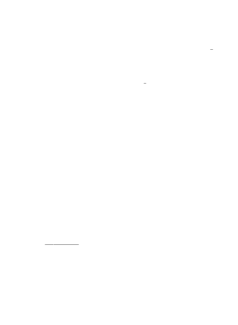
with tD"¸2/p2D. In the general case, g is replaced by (b/2)g here. Eq. (4.33) is completely

analogous to the formula (3.42), (3.43) for the statistics of eigenfunction amplitudes. It shows that
the correction to the leading term !t/tD in lnPS becomes large compared to unity at tZJgtD,

though it remains small compared to the leading term up to t&gtD&D~1.

Result (4.33) was also obtained by Frahm [151] from rather involved calculations based on the

equivalence between the 1D

p-model and the Fokker

}Plank approach and employing the approx-

imate solution of the Dorokhov}Mello}Pereyra}Kumar equations in the metallic limit. The fact
that the logarithm of the quantum decay probability, ln PS(t), starts to deviate strongly (compared

to unity) from the classical law, ln P

#-s(t)"!t/tD at t&tDJg was observed in numerical simula-

tions by Casati et al. [152]. For related results in the framework of the random matrix model see
Section 4.1.3.

4.1.2. 2D geometry

We consider now a 2D disk-shaped sample of a radius R with an open boundary. If the problem

is formulated in terms of the conductance, we can assume the two leads attached to the disk
boundary to be of almost semicircular shape, with relatively narrow insulating intervals between
them. Then we can approximate the boundary conditions by using Eq. (4.6) for all the boundary. In
fact, in view of the logarithmic dependence of the saddle point action on R (see below), the result
does not depend to the leading approximation on the speci"c shape of the sample and the leads
attached. With the rotationally invariant form of the boundary condition, the minimal action
corresponds to the function

h depending on the radial coordinate r only. We get therefore the radial

equation

hA#h@/r#2c sinh h"0, 04r4R

(4.34)

(the prime denotes the derivative d/dr) with the boundary conditions:

h(R)"0 ,

(4.35)

h@(0)"0

(4.36)

Condition (4.36) follows from the requirement of analyticity of the "eld in the disk center.

Assuming that characteristic values of

h satisfy the condition h<1 (which corresponds to

D<1), one can replace sinh h by eh/2. Eq. (4.34) can be then easily integrated, and its general

solution reads:

h(r)"

C2rC

(C2rC

(4.37)

with two integration constants C1 and C2. To satisfy the boundary condition (4.36), we have to

choose C1"2. Furthermore, the above assumption h(0)<1 implies that 2C2/c<1. Therefore, the

second boundary condition (4.35) is satis"ed if C2K8/cR4, and the solution can be written in the

form

h(r)K[(r/R)2#cR2/8]~2 .

(4.38)

299

A.D. Mirlin / Physics Reports 326 (2000) 259}382

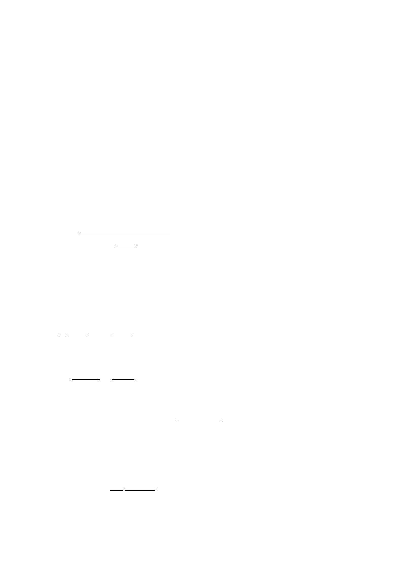
Using now the self-consistency equation (4.9) one "nds

c"4p2l/t. Finally, calculating the action

on the saddle point (4.38), we "nd [29]

ln Ps(t)"SK8p2lDln(tD) ,

(4.39)

The above treatment is valid provided

h@(r)(l~1 on the saddle point solution, which is the

condition of the applicability of the di!usion approximation (here l is the mean free path). In
combination with the assumption

h(0)<1 this means that 1;tD;(R/l)2.

Now let us consider the region of still longer times, t<

D~1(R/l)2. In order to support the

applicability of the di!usion approximation, we should search for a function

h(r) minimizing the

action with an additional restriction

h@4Al~1. Here A is a parameter of the order of unity, which

cannot be "xed within the di!usion approximation. We will see however that the saddle-point
action depends on l through ln(R/l) only, and thus does not depend on A in the leading order, so
that we can set A"1. Since the derivative has a tendency to increase in the vicinity of r"0, the
restriction can be implemented [30] via replacing the boundary conditions (4.36) by

h@(r

H )

where the parameter r

H will be speci"ed below. The solution reads now:

h(r)"

(r/R)

C~2

(r/R)

C#2
C!2

H /

;

r4R .

(4.40)

The function

h(r) is meant as being constant within the vicinity DrD4r

H of the disk center. The

condition

h@4l~1 yields r

lC. It is important to note that the result does not depend on details

of the cut-o! procedure. For example, one gets the same results if one chooses the boundary
condition in the form

h@(r

H )

1/l. The crucial point is that the maximum derivative

h@ should not

exceed 1/l. The constant C is to be found from the self-consistency equation (4.9) which can be
reduced to the following form:

p2lR2

C!2

(4.41)

Neglecting corrections of the ln(ln ) ) form, we "nd

ln(t

ln(R/r

H )

ln(t

ln(R/l)

(4.42)

The action (4.10) is then equal to

p2lD(C#2)2 ln(R/r

H )

p2lD

2[tD(R/l)2]

ln(R/l)

(4.43)

Combining Eqs. (4.39) and (4.43) and introducing the factor

b/2 for generality, we get thus the

following long-time asymptotics of Ps(t) (or G(t)) [30]:

Ps(t)&(tD)~2pbg, 1;tD;(R/l)2 ,

(4.44)

Ps(t)&exp

pbg

2 (t/gq)

ln (R/l )

D<(R/l)2 ,

(4.45)

A.D. Mirlin / Physics Reports 326 (2000) 259}382

300

where g"2

plD is the dimensionless conductance per square in 2D and q is the mean free

time.

The far asymptotic behavior (4.45) is of the log-normal form and very similar to that found by

AKL (see Eq. (7.8) in Ref. [28]). It di!ers only by the factor 1/g in the argument of ln

2. It is easy to

see however that this di!erence disappears if one does the last step of the AKL calculation with
a better accuracy. Let us consider for this purpose the intermediate expression of AKL (Ref. [28],
Eq. (7.11)):

G(t)J!

~t@t

(

exp

(

(4.46)

where

p2lD

in the weak localization region in 2D, which we are considering. Evaluating the integral (4.46) by
the saddle point method, we "nd

G(t)&exp

2ut

exp

2(t/gq)

ln(R/l)

(4.47)

where we have kept only the leading term in the exponent. Eq. (4.47) is in exact agreement with
Eq. (4.45) for

b"1 (AKL assumed the orthogonal symmetry of the ensemble). Therefore, the

supersymmetric treatment con"rms the AKL result and also establishes the region of its validity. It
is instructive to represent the obtained results in terms of the superposition of simple relaxation
processes with mesoscopically distributed relaxation times t

(

G(t), Ps(t)&

(

~t@t

(

P(t

(

) .

(4.48)

Eqs. (4.44) and (4.45) lead then to the following result for the distribution function P(t

(

) [30]:

P(t

(

/tD)~2pbg,

tD;t

(

;

tD(R/l)2 ,

exp

pbg

2(t

(

ln(R/l)

(

tD(R/l)2 ,

(4.49)

where tDKR2/D is the time of di!usion through the sample.

The smooth envelope of the ALS corresponding to the intermediate region tD;t

(

;

tD(R/l)2

has according to Eq. (4.37) the following spatial structure:

Dt2(r)D4.005)"N~1eh(r)"

bpDt

(

[(r/R)

2#R2/8bDt

(

]

(4.50)

301

A.D. Mirlin / Physics Reports 326 (2000) 259}382

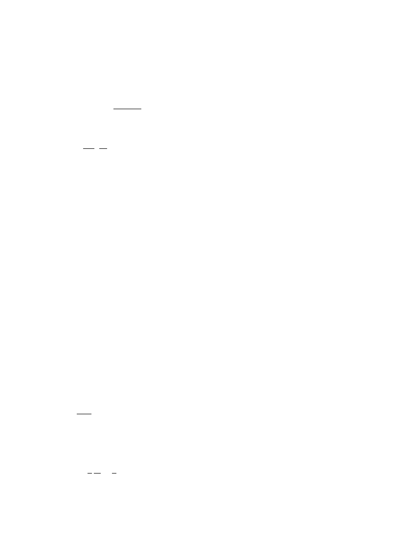
Thus, this ALS has an e!ective localization length

m%&&R(tD/t

(

)

1@2, with the intensity decreasing as

1/r

4 outside the region of the extent m%&. As to the ultra-long-time region, Eqs. (4.40) and (4.42)

indicate that now the e!ective localization length is given by l

(t)

H de"ned as

(t)

ctl;

ctK

ln(t

(

/tD)

ln(R/l)

(4.51)

The ALS intensity decays in a power-law manner for r'l

(t)

H , with an exponent depending on

(

Dt2(r)D&

(t)2

(t)

r4R .

(4.52)

4.1.3. Random matrix model

Here we mention brie#y the results on the quantum decay law obtained by Savin and Sokolov

[153] within the RMT model. This will allow us to see the similarities and the di!erences between
the di!usive systems and the random matrix model. The model describes a Hamiltonian of an open
chaotic system by a Gaussian random matrix coupled to M external (decay) channels. The decay
law found has the form

Ps(t)&(1#CWt/M)~M ,

(4.53)

where

CW"M¹D/2p is a typical width of the eigenstate, with ¹ characterizing the channel

coupling (¹"1 for ideal coupling, see also Section 6). In this case, the product M¹ plays a role of
the dimensionless conductance g (in contrast to the di!usive case where g is governed by the bulk
of the system, here it is determined by the number of decay channels and the strength of their
coupling). For not too large t (t

*¹;1), Eq. (4.53) yields the classical decay law, Ps(t)&e~t

, with

the corrections of the form

ln Ps(t)"!tCW(1!CWt/2M#2) ,

(4.54)

which is similar to the results found for the di!usive systems (see, e.g. Eq. (4.33)). At large
t<(

*¹)~1, the decay take the power-law asymptotic form [154]

ln Ps(t)K!M ln(CWt/M) .

(4.55)

4.1.4. Distribution of total density of states

Here we discuss the contribution of ALS to the asymptotic behavior of the distribution function

l) of the total density of states (DOS),

l(E)"

dr GR(r,r;E)

(4.56)

(in the present subsection we denote the average DOS as

l0 to distinguish it from the #uctuating

quantity

l(E)). A resonance state with an energy E and width t~1

(

gives a following contribution

l(E):

lALS(E)"

2
p

(

2
p

(

Dl0 .

(4.57)

A.D. Mirlin / Physics Reports 326 (2000) 259}382

302

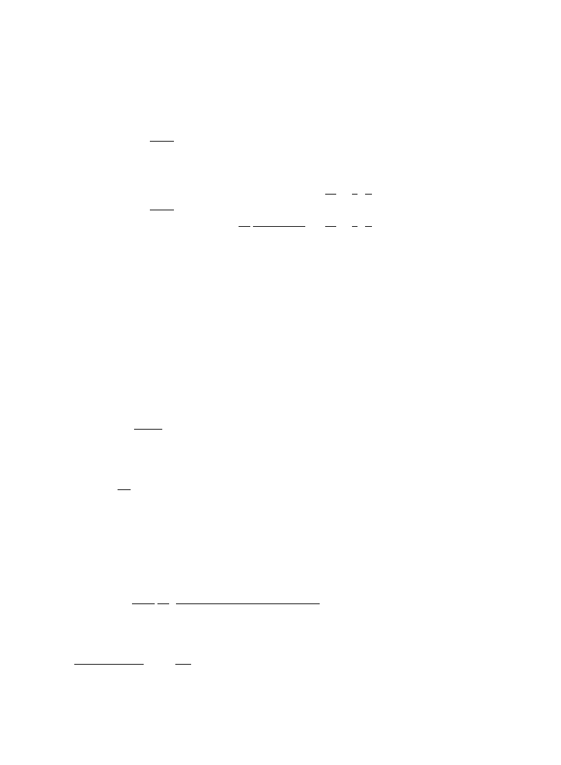
We expect that the asymptotic behavior of P(

l) at l<gl0&tD/< is determined by a single

anomalously localized states with t

(

tD. This yields [36]

l)&P

(

Dl0

exp

M!g ln2(gl/l0)N .

(4.58)

in the quasi-1D case and

l)&P

(

Dl0

l/l0)~4pg,

;

1
g

exp

2(l/l0*q)

ln(¸/l)

1
g

(4.59)

in the 2D geometry. The far LN asymptotic tail in Eq. (4.59) is in full agreement with the RG
calculation by Altshuler et al. [28]. We "nd also an intermediate power-law behavior, which could
not be obtained from the study of cumulants in Ref. [28]. We note, however, that this power-law
form is fully consistent with the change of the behavior of cumulants

|ln} at n&pg discovered

in [28].

4.2. Distribution of eigenfunction amplitudes

4.2.1. Quasi-1D geometry

The spatial shape of the ALS determining the asymptotics of the distribution function of

eigenfunction intensities can be found [36] via the exact solution of the

p-model. We de

"ne

SDt2(r)DTu"

Q(u, r)

P(u)

(4.60)

where

Q(u, r)"

Dta(r)D2d(Dta(0)D2!u)d(E!Ea)

(4.61)

and P(u) is the distribution function of u"

Dt2(0)D de

"ned formally by Eq. (3.3). According to

Eq. (4.60),

SDt2(r)DTu is the average intensity of an eigenstate, which has in the point r"0 the

intensity u (which will be assumed to be atypically large). The exact result for P(u) is given in the
form of the Lebedev}Kontorovich expansion by Eqs. (3.12), (3.21) and (3.24). Calculating
the moments

SDt(0)D2Dt(r)D2qT, and restoring the function Q(u, r), we

"nd for r'l

Q(u, r)"!

(2)(umA; q1,q2)=(1)(umA,q~)

(4.62)

where the function =

(2)(z; q1,q2) satis"es the same equation, as =(1),

R=(2)(z; q1, q2)

Rq1

2 R

Rz2

(2)(z; q1,q2)

(4.63)

303

A.D. Mirlin / Physics Reports 326 (2000) 259}382

with the boundary condition

(2)(z; 0, q2)"z=(1)(z,q2) .

(4.64)

The solution of Eqs. (4.63) and (4.64) is

(2)(z, q1,q2)"2Jz

k b(k, q2)Kik(2Jz)e~((1`k

)@4)q

k, q2)"

k sinh(pk)

dt Kik(t)=(1)(t2/4,q2) .

(4.65)

Substituting here the formula (3.24) for =

(1)(z, q2) and evaluating the integral over z, we can reduce

Eq. (4.65) for b(

k, q2) to the form

k, q2)"

k sinh(pk)

1#i

(1#

k2)#

k sinh(pk)

k1k1

k21

]sinh

pk1

1#i

k#k1

1#i

k!k1

~((1`k

)@4)q

(4.66)

In the opposite case r(l we "nd

Q(u, r)"

kd(r)

>a(u) ,

(4.67)

where the function >a(u) was de"ned in Eq. (3.9). This formula is valid for any sample, which is

locally d-dimensional. In the case of the quasi-1D geometry we get

Q(u, r)"

kd(r)

(1)(umA, q~)=(1)(umA,q`)], r;l

(4.68)

4.2.1.1. Insulating sample (¸<

m). The distribution P(u) is given by Eqs. (3.45) and (3.46). The

`taila, Eq. (3.47), at u<1/Am corresponds to atypically large local amplitudes. Analyzing the
general formula for

SDt2(r)DT in this case, we

"nd [36] the following spatial structure of the ALS

with

Dt2(0)D"u:

SDt2(r)DTu"

p3@2

~1@2A~3@2r~3@2e~r@4m, r<m ,

(4.69)

SDt2(r)DTu"

1
2

1@2

1#r

l(r;

m ,

(4.70)

SDt2(r)DTu"

1
2

1@2

[1#2

JuAmkd(r)], r(l .

(4.71)

We see from Eqs. (4.69), (4.70) and (4.71) that the eigenfunction normalization is dominated by the
region r&

m%&, where m%&&Jm/uA;m plays the role of an e!ective localization length. In the

A.D. Mirlin / Physics Reports 326 (2000) 259}382

304

region

m%&;r;m the wave intensity falls down as 1/r2, and crosses over to the conventional

localization behavior at r<

m. Therefore, the appearance of an anomalously high amplitude

Dt2(0)D"u<1/Am is not just a local

#uctuation, but rather a kind of a cooperative phenomenon

corresponding to existence of a whole region r

[m%& with an unusually large amplitude

Dt2(r)D"12Ju/mA&1/Am%&.

Eq. (4.71) describes a sharp drop of the amplitude from

Dt2(0)D"u to SDt2(r)DT"12Ju/mA

at r&l. This

`quasi-jumpa happens on a short scale r0&k~1

(uA

m)1@*2(d~1)+. To understand

the reason for it, let us recall that the above formulas represent the average intensity

Dt2(r)D (under

the condition

Dt2(0)D"u). One can also study the

uctuations of the intensity. It turns out [36] that

in the region r0;r;m the #uctuations are of usual GUE type superimposed on the envelope

(4.70). It is not di$cult to understand that the quasi-jump has the same origin as the GUE-like

#uctuations at r<r

. One can ask, of course, why this short-scale #uctuation happens exactly in

the center of the smooth ALS

`bumpa with a probability close to unity. The answer is as follows.

We are studying the states with an anomalously large local intensity u, which is an exponentially
rare event. There are two sources which may favor the formation of such a high intensity:
(i) formation of an ALS with a spatially non-uniform smooth envelope, and (ii) short-scale
GUE-like #uctuations. Both these mechanisms have exponentially small probabilities to produce
an enhancement of the intensity by a large factor. The found con"guration of

SDt2(r)DTu (short-scale

quasi-jump (4.71) on top of the smooth con"guration (4.70)) represents just the optimal combination
of the two mechanisms:

Dt2(0)D4.005) J(u),

1
2

1@2

2(uA

m)1@2 .

(4.72)

For arbitrary geometry of the sample, the magnitude of the

`quasi-jumpa J(u) is given according to

Eq. (4.67) by

J(u)K!u

ln>a(u)K!u

ln P(u)

(4.73)

(in the quasi-1D case this reduces to J(u)"2(uA

m)1@2 as stated above). The formula (4.73) can be

reproduced (within the saddle-point approximation) by writing the quantity u as a product u"usJ

of the smooth part us and the local #uctuating quantity J, with the latter distributed according to

P(J)"e

~J.

4.2.1.2. Metallic sample (¸;

m). The asymptotic behavior of the intensity distribution function

has the same stretched-exponential form, as in the localized regime, see Eq. (3.44). More accurately
(with the subleading factors included), this formula reads [36]

P(u)"

16
p2

J¸`¸~

exp

JumA#

p2m

4¸`

Jm/uA

¸`

p2m

4¸~

Jm/uA

¸~

(4.74)

Calculation of Q(u, r) shows [36] that the ALS intensity has for l(r;¸ the same form (4.70),
provided the condition <

Dt2(0)D<g is ful

"lled.

This condition, under which the asymptotic

305

A.D. Mirlin / Physics Reports 326 (2000) 259}382

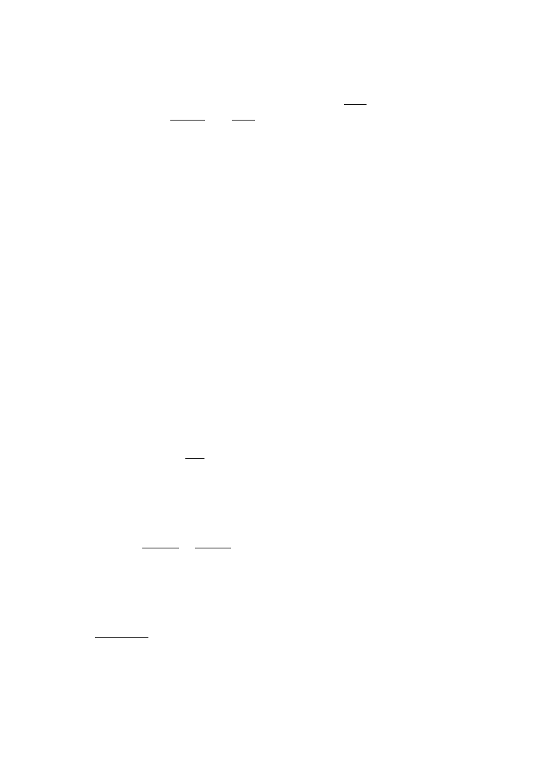
behavior (3.44), (4.74) is valid, acquires now a very transparent meaning. This is just the condi-
tion that the e!ective localization length of an ALS,

m%&"Jm/uA is much less than the sample

size ¸. Indeed,

m%&/¸"Jm/uA¸2"Jg/u<.

Near the sample edges, r&¸<

m%&, the form of the ALS intensity is slightly modi"ed by the

boundary of the sample, see [36]. Finally, the

`quasi-jumpa of SDt2(r)DTu at r;l has the same form

(4.71) as in the insulating regime.

4.2.1.3. Saddle-point method. The saddle-point method of Muzykantskii and Khmelnitskii can be
also applied to the problem of the statistics of eigenfunction amplitudes, as was done by Fal'ko and
Efetov [32,33]. In this case, one should look for the saddle-point of the functional integral (3.8)
determining the function >a(u) (which in turn determines the eigenfunction statistics, see Eqs. (3.12)

and (3.14)). The saddle-point is again parametrized by the bosonic non-compact angle

h(r) only,

and the corresponding saddle-point equation has the form

plD+2h!ueh"0 .

(4.75)

It is similar to Eq. (4.8) of the long-time relaxation problem, but with di!erent sign of the second
term. Also, the boundary conditions have now a di!erent form:

h(0)"0

(4.76)

and condition (4.7) at the boundary (since we consider now a closed sample). Alternatively, one can
write Eqs. (4.75) and (4.76) in a slightly di!erent form by shifting the variable

h#ln(u<)Ph. Then

u is removed from the saddle-point equation and from the action, but appears in the boundary
condition.

The action determining the distribution function P(u) is given by

ln P(u)"S"

plD

(

+h)2#ueh

(4.77)

The formula (4.77) acquires a very transparent meaning if we take into account what was written
in Section 4.2.1 concerning the two factors contributing to the large amplitude

Dt2(0)D"u. Firstly,

this is the non-uniform smooth envelope Je

) yielding

Dt2(0)D4.005)"

h(0)

:ddr eh(

)

:ddr eh(

)

the corresponding weight is represented by the "rst term in action (4.77). Secondly, these are the
local Gaussian (GUE-like) #uctuations of the wave function amplitude, which should provide the
remaining factor (

`quasi-jumpa)

Dt2(0)D4.005)

dr eh(

) ,

the corresponding probability P(J)"e

~J reproduces the second term in action (4.77).

A.D. Mirlin / Physics Reports 326 (2000) 259}382

306

In the quasi-1D case and under the condition u<g<

~1, the solution of Eq. (4.75) reads [33,34]

h(r)"

1#r

plD

0(r;¸` .

(4.78)

Comparing Eq. (4.78) with Eqs. (4.70), we see that the saddle-point solution nicely reproduces the
average intensity of the ALS,

SDt2(r)DTu for r'l, up to an overall normalization factor. Also,

the form of P(u) found in the quasi-1D case by the saddle-point method [33] is in a very good
agreement with the exact results presented above. This agreement does credit to the saddle-point
method and allows to use the saddle-point con"guration for characterizing the shape of ALS in
higher dimensions and for other distribution functions, where the exact solution is not available.

4.2.2. 2D geometry

For a 2D disk-shaped sample of a radius ¸ with the high amplitude point r"0 in the center of

the disk, the saddle-point solution of Eqs. (4.75) and (4.76) is found to have the form [32,33]

h(r)"

~2k

8(1!

k)2plD

2~2k

r5l

~2k

for l

r;¸ ,

(4.79)

where the exponent 0(

k(1 depends on u and satis

"es the equation

k(1!k)2

plD

(4.80)

We are interested in the asymptotic region u¸

2<plD ln~1(¸/l ), where the distribution of the

eigenfunction intensity is given by Eq. (3.58), and an ALS is formed. Then the exponent

k can be

approximated as

plD

2 ln(¸/l

H )

(4.81)

The lower cut-o! scale l

H appears in Eq. (4.79) for the same reason as in the long-time relaxation

problem (Section 4.1.2), i.e. because of the restriction of the di!usion approximation on the
momenta q of the

p-model

"eld: q(l

~1. It is determined by the condition h(@r)Dr/l

~1, which

yields l

kl. The corresponding asymptotic behavior of >a(u) (and consequently of the intensity

distribution function), which was already quoted in Section 3.3.1, is

>a(u),P(u)&exp

p2lD

ln(¸/l

H )

(4.82)

307

A.D. Mirlin / Physics Reports 326 (2000) 259}382

Normalizing the expression (4.79), we "nd that the average ALS density for r'l

H is equal to

SDt2(r)DTu"

p2lDk

~2k

8(1!

k)2plD

2~2k

r5l

H .

(4.83)

The saddle-point calculation assumes that

h(r) is constant for r(l

H , so that Eq. (4.83) gives

SDt2(r)DTuK

p2lDk

in this region. However, for very small r(l the average intensity

SDt2(r)DTu changes sharply, as we

have seen in the quasi-1D case. Using Eq. (4.67) for Q(u, r) and Eq. (3.12) for P(u), we get

SDt2(r)DTu,

Q(u, r)

P(u)

[1!k2(r)#J(u)k2(r)]SDt2(r"lH)DTu, r(lH .

(4.84)

According to Eqs. (4.73) and (4.82), the height of the quasi-jump is given by

J(u)K!u

ln>a(u)K

p2lD

ln(¸/l

H )

p2lD

p2lDk ,

(4.85)

which is precisely the factor by which the value of

SDt2(r"l

H )DT

found above di!ers from

SDt2(0)DTu,u. Combining Eqs. (4.83)}(4.85), we get

SDt2(r)DTu"

J(u)

[1!k2(r)#k2(r)J(u)], r(lH .

(4.86)

Therefore, in the 2D case the ALS determining the asymptotics of the amplitude distribution
function has the power-law shape (4.83) with the short-scale bump (4.86).

4.2.3. States localized near the boundary

We assumed in the above calculations that the center of an ALS is located far enough from the

sample edge. For a quasi-1D sample, this means that

m%&;¸`,¸~. In the 2D case this implies that

the distance from the observation point to the boundary is of the same order of magnitude in all
directions, so that ln(¸/l) is de"ned without ambiguity. Here, we will consider brie#y the role of
ALS situated close to the boundary, when these conditions are violated [36].

We "rst consider the quasi-1D geometry. Let us calculate the distribution function P(u) in

a point located very close to one of the sample edges. Formally, this means that ¸~;m%&. Then the

function =

(1)(uAm, q~) in Eq. (3.21) can be approximated by unity, and we get

P(u)"

2
p

m3@4A1@4¸~1@2u~3@4 exp

JumA#

p2m

4¸`

Jm/uA

¸`

(4.87)

We see therefore that close to the boundary the distribution P(u) has the asymptotic decay
P(u)&exp

M!2JuAmN, which is slower than in the bulk of the sample, P(u)&expM!4JuAmN.

This means that if we consider the distribution P(u) averaged over the position of the observation
point, its asymptotic tail will be always dominated by contribution of the points located close to the

A.D. Mirlin / Physics Reports 326 (2000) 259}382

308

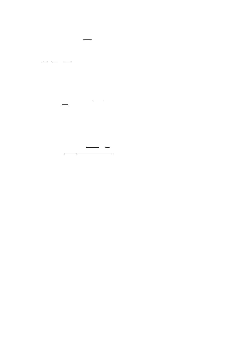
boundary, P(u)&exp

M!2JuAmN. This could be already anticipated from Eq. (4.74), where the

factor

exp

¸`

¸~

increases strongly with approaching one of the sample edges. The same tendency, but in a weaker
form, is observed in Eqs. (3.40)}(3.43). Calculating the average intensity

SDt2(r)DTu of the corre-

sponding ALS, we "nd that at r'l the ALS spatial shape retain the form (4.70), with an additional
overall factor of 2. At small r, Eq. (4.71) is slightly modi"ed:

SDt2(r)DTu"

1@2

[1#

JuAmkd(r)] .

(4.88)

In 2D, we can consider a sample of the semicircular shape, with the observation point located in

the center of the diameter serving as a boundary. The saddle-point solution then has exactly the
same form (4.79), and the ALS intensity is still given by Eq. (4.83), with an additional factor 2. The
asymptotic form of the distribution function P(u) contains an extra factor 1/2 in the exponent:

P(u)&exp

p2lD

ln(¸/l

H )

(4.89)

This result is expected to be applicable to any 2D sample of a characteristic size ¸, with a smooth
boundary and the observation point taken in the vicinity of the boundary.

We see therefore, that, very generally, the probability of formation of an ALS with the center in

a given point is strongly enhanced (via an extra factor 1/2 in the exponent), if this point lies close to
the sample edge. This leads to the additional factor 1/2 in the exponent in the asymptotic form of
the distribution P(u) near the boundary.

4.3. Distribution of local density of states

We again assume the sample to be open, as in the problem of the distribution of relaxation times,

Section 4.1. Then it is meaningful to speak about the statistics of the local density of states (LDOS)
o(E, r)"(!1/p)Im GR(r,r;E). In a metallic sample, the LDOS is a weakly #uctuating quantity,

whose distribution P(

o) is mostly concentrated in a narrow Gaussian peak [28,155] with mean

value

SoT"l and the variance var(o/l)&i;1, where i is the usual parameter of the perturba-

tion theory

i"P(r, r)"

pl<Dq2, which already appeared in Section 3.3.1. This close-to-

Gaussian shape of P(

o) holds however in the region Do/l!1D;1 only. We will consider in contrast

the

`tailsa of the distribution, o/l;1 and o/l<1, where a much slower decay of P(o) will be

found.

We begin by discussing on a qualitative level a relation of the asymptotics of P(

o) to the behavior

of the distribution functions considered above. Typically, in an open metallic sample the LDOS
o(E, r) is given by a superposition of &1/tDD"g adjacent levels, since their widths are of order

of 1/tD. However, we can expect that for o much larger than its average value l, the asymptotic form

309

A.D. Mirlin / Physics Reports 326 (2000) 259}382

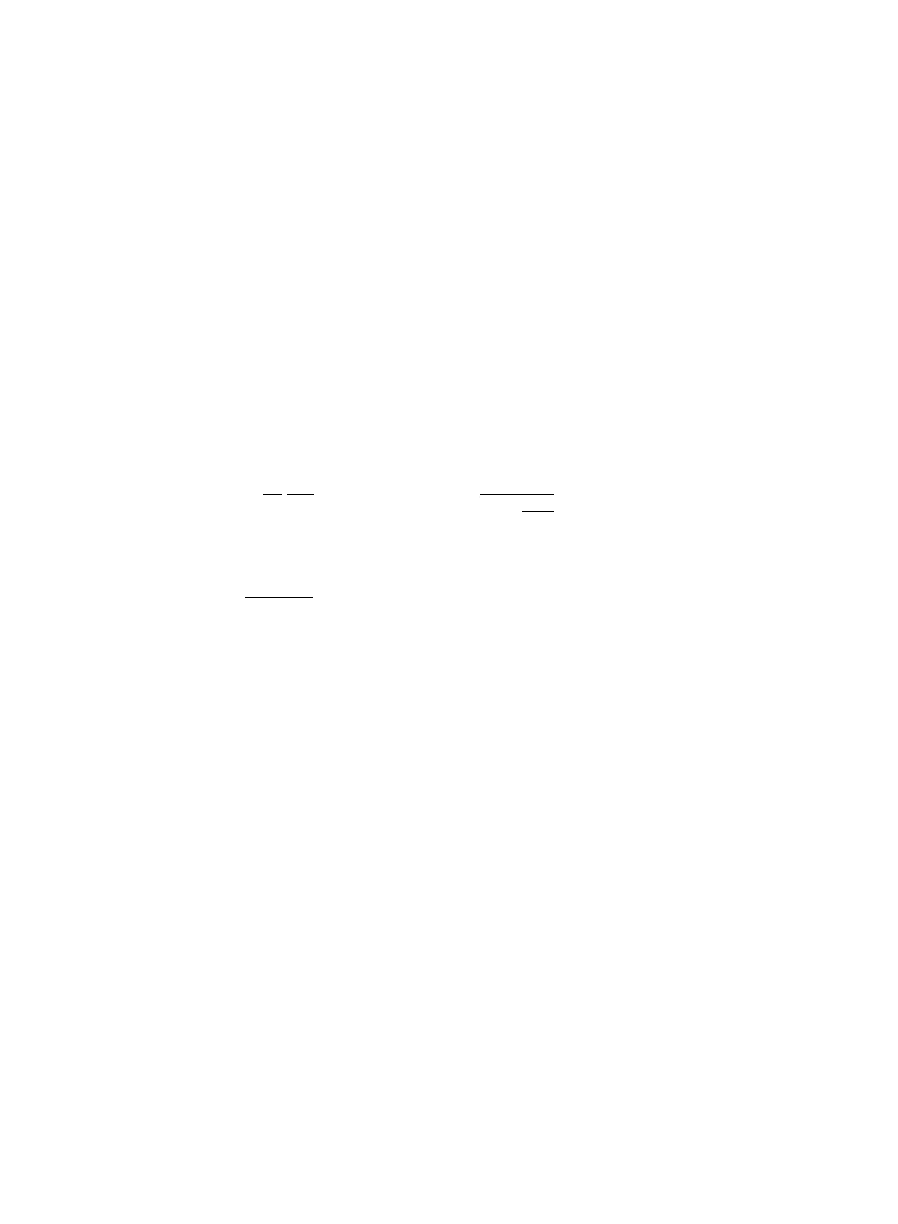
of P(

o) is determined by a probability to have a single narrow resonance, which gives this value of

LDOS

o(E, r). The most favorable situation happens when the resonance is located around the

point r in the real space and around the energy E in energy space. The LDOS provided by such
a resonance is:

oALS"Dt2(r)D2t

(

p ,

(4.90)

where t

(

is the resonance width. Thus, the optimal #uctuation should provide now a maximum to

the product of the local amplitude u"

Dt2(r)D and the inverse level width t

(

, and the asymptotics of

the distribution P(

o) should be related to that of P(u) and P(t

(

). In particular, in the quasi-1D case,

where the distribution P(t

(

), Eq. (4.25), decays much more slowly than P(u), Eq. (3.47), one should

expect the asymptotic behavior of P(

o) to be mainly determined by P(t

(

). We will see below that

this is indeed the case.

Now we turn to a formal calculation. The distribution function P(

o) of LDOS can be expressed

through the function >(

j1,j2) introduced in Section 3.1 as follows [19,20,322,323].

o)"d(o!1)#

Ro2

`1)@2o

j1 >M(j1)

j1!o

1@2

(4.91)

where

M (j1)"

(

j1,j2)

j1!j2

(4.92)

and

o is normalized by its mean value: o/lPo. Let us note the symmetry relation found in [19,20]

o~1)"o3P(o) .

(4.93)

It follows from Eq. (4.91) and is completely independent of a particular form of the function
>

(

j1,j2). Obviously, Eq. (4.93) relates the small-o asymptotic behavior of the distribution P(o) to

its large-

o asymptotics.

Asymptotic behavior of P(

o) was studied in [34] via the saddle-point method supplemented in

the quasi-1D case by the exact solution. The saddle-point equation has for this problem a very
simple form,

+2h"0 ,

with the boundary conditions

hD-%!$4"0, h(0)"o/2 .

4.3.1. Quasi-1D geometry

In the quasi-1D case, the solution reads

h(r)K

(

o/l)1~r@L

r'0 ,

(

o/l)1~@r@@L

r(0 ,

(4.94)

A.D. Mirlin / Physics Reports 326 (2000) 259}382

310

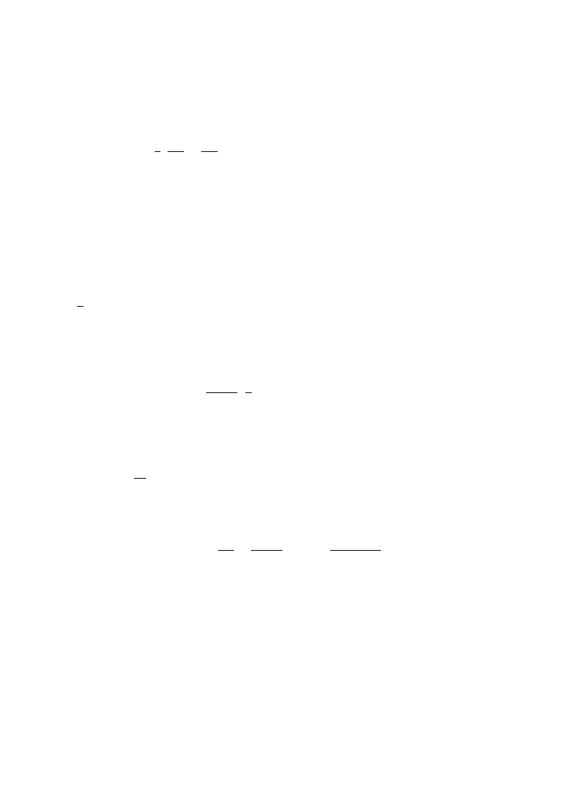
where, as before, ¸` and ¸~ are the distances from the observation point r"0 to the sample

edges. This yields the asymptotics of the distribution function

o)&exp

m
4

¸`

¸~

2(o/l)

(4.95)

Let us note that this asymptotic behavior of P(

o) in an open sample is strongly di

!erent from the

asymptotics of P(u) in a closed sample, Eq. (3.47). As was explained above, the di!erence originates
from the fact that P(

o) is essentially determined by P(t

(

). To demonstrate this explicitly, we put the

observation point in the middle of the sample, ¸`"¸~"¸/2. The con"guration (4.94) acquires

then precisely the same form as the optimal con"guration (4.19) for the relaxation time t

(

, and the

asymptotics (4.95) of P(

o) is identical to that of P(t

(

), Eq. (4.25).

The corresponding values of t

(

and

o are related as follows:

(

2(gDt

(

o/l .

(4.96)

Now we calculate the value of the local amplitude

Dt2(0)D for an ALS corresponding to the

con"guration (4.94). First, its smoothed intensity is given by

Dt2(r)D4.005)"N~1eh(r)"

ln(

o/l)

~2@r@@L

(4.97)

Second, the quasi-jump induced by the GUE-type #uctuations gives an additional factor, which is
found according to Eq. (4.73) to be

o)"!o R

ln P(

o)"2g ln(o/l) .

(4.98)

Combining Eqs. (4.96)}(4.98), we can compute the LDOS (4.90) determined by this resonance state:

oALS(E,0)"Dt2(0)D4.005) J(o)

(

ln(

o/l)

2g ln(

o/l)

2g ln

2(o/l)

o .

(4.99)

We have explicitly checked therefore that the LDOS

o is indeed determined by a single ALS,

smoothed intensity of which is given by Eq. (4.97). There are three sources of the enhancement of
LDOS: (i) amplitude of the smooth envelope of the wave function, (ii) the short-scale GUE

`bumpa,

and (iii) the inverse resonance width. They are represented by the three factors in Eq. (4.99),
respectively.

The result (4.95) can be also obtained [34] from the exact solution of the

p-model. It was also

shown in [34] that in the long wire limit (¸<

m) the whole distribution function takes a log-normal

form analogous to that found in [113] for the case of a strictly 1D sample by the Berezinskii
technique.

311

A.D. Mirlin / Physics Reports 326 (2000) 259}382

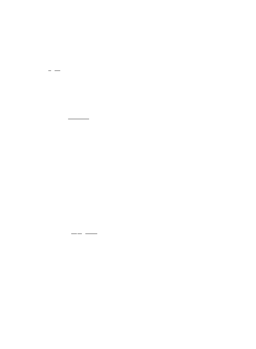
4.3.2. 2D geometry

In the 2D case, we introduce again (as in Sections 4.1.2 and 4.2.2) the small-r cuto!, l

(o)

H . The

saddle-point solution reads

h(r)K

(o)

(4.100)

where l

(o)

col, and

co"ln(o/l)/ln(¸/l(o)H) .

The distribution P(

o) has the following asymptotics [34]:

o)&exp

p2lD ln2o

ln(¸/l

(o)

H )

(4.101)

So, the LDOS distribution has (as in the quasi-1D case) the log-normal form, which is now similar
to the distribution (4.82) of the eigenfunction intensities (while the distribution of relaxation times
has an intermediate power-law regime). This result is in perfect agreement with the asymptotic
behavior of P(

o) found by the renormalization group method in [28].

As for all the other distribution functions studied, the relevant ALS decay in a power-law

fashion,

Dt2(r)DJ(r/l(o)

H )~c

. Like in the quasi-1D case, one can explicitly verify [36] that a single

state with the spatial shape determined by (4.100) indeed provides, by virtue of Eq. (4.90), the value
of LDOS equal to

4.4. Distribution of inverse participation ratio

In this subsection, we study the asymptotics of the distribution function of the IPR P2, Eq. (3.39).

We have already considered the #uctuations of P2 in Section 3.3.3. As was explained there, the

relative magnitude of the #uctuations is [r.m.s.(P2)]/SP2T&1/g. At 1/g;P2/SP2T!1;1 the

distribution function is of the exponential form,

P(P2)&exp

SP2T

(4.102)

Note that for negative deviations P2/SP2T!1 with DP2/SP2T!1D<1/g the distribution function

decays much faster [137], so that the distribution is strongly asymmetric. As was mentioned in
Section 3.3.2, the

`bodya of the distribution P(P2) is described properly (in the leading order in 1/g)

by the Liouville theory. We will see below that this is also true for the asymptotic

`taila of P(P2).

Our consideration of asymptotics of the IPR distribution is based on unpublished results [35]

(partially announced in [36]). We derive "rst a relation between P(P2) and the distribution of level

velocities Pv(v) [25]. To this end, we consider a Hamiltonian H#aW, where W is a random

perturbation. Speci"cally, the matrix elements Wr

are supposed to be independent Gaussian-

distributed random variables with the mean value equal to zero and the variance

SWHr

T"W0(Dr1!r2D)d(r1!r@1)d(r2!r@2) .

A.D. Mirlin / Physics Reports 326 (2000) 259}382

312

We will assume that W0(r) is a short-ranged function with some characteristic scale f. The level

velocity vn corresponding to an energy level En is de"ned as vn"dEn(a)/da (where En(a) is the level

of the perturbed Hamiltonian H#

aW) and can be found within the conventional perturbation

theory as

vn"

dr@ Wrr{tHn(r)tn(r@) .

(4.103)

Using (4.103), we "nd

Sv2nT"w0P2,

w0"c

dr W0(r) ,

(4.104)

where c"1 (1/2) if kff;1 (resp. kff<1).

This consideration can be extended to higher moments of the level velocity

Sv2q

n T

as well. This

leads to the following relation between the two distributions:

Pv(v),Sd(v!vn)T

dP2

pw0P2]1@2

exp

2w0P2

PI(P2) .

(4.105)

On the other hand, the level velocity distribution can be expressed through the

p-model correlation

function in the following way [156]. According to the de"nition,

Pv(v)"

d(E!En)d(v!REn/Ra)

a?0

lim

a?0

d(E!En(0))d(E#av!En(a))

(4.106)

so that Pv(v) is determined by the aP0 limit of the parametric level correlation function. The latter

can be represented [as a generalization of Eq. (2.10)] in terms of a correlation function of the
p-model [157

}159]. This yields

Pv(v)"lim

g?0

l<v

dr Str Q11k

BAP

dr Str Q22k

*Q+;

Sv[Q]"

dr Str

plD

(

+Q)2!

plg

w0(pl)2g2

KQK

(4.107)

Combining Eqs. (4.105) and (4.107), we "nd the expression for the IPR distribution function in
terms of the

p-model,

PI(P2)"

J2pP3@2

lim

g?0

gl<

c`*=

c~*=

]

dr Str Q11k

BAP

dr Str Q22k

*Q+ ;

(4.108)

313

A.D. Mirlin / Physics Reports 326 (2000) 259}382

where Su[Q]"!u/2P2#Sv[Q]Dv

. The saddle point con"guration is again parametrized by

the bosonic

`anglea h(r) only; the action on such a con"guration is

Su[h]"!

2P2

plD

(

+h)2!

plg

(

plg)2

(4.109)

The corresponding saddle-point equations can be readily obtained by varying Su[h] with respect to

h(r) and u:

+2h!

plg2

2h"0,

(

plg)2

dr e2h#

2P2

0 .

(4.110)

Making a shift

h"hI#ln(iu/plg) and dropping the tilde, we can reduce them to the form

+2h!c(eh!e2h)"0 ,

(4.111)

P2"2

dr e2h ,

(4.112)

where

c"u/2plD. Integration of Eq. (4.111) with the Neumann boundary condition yields

:ddr(eh!e2h)"0, so that Eq. (4.112) can be rewritten in the following form (invariant with respect
to a shift of the variable

h):

P2"2

:ddr e2h

(

:ddr eh)2

(4.113)

The meaning of Eq. (4.113) is completely transparent if we recall that

Dt2(r)D4.005)Jeh(

). The factor

2 comes from the GUE-like short-scale #uctuations.

Taking into account Eqs. (4.111) and (4.112), we "nd the action (4.109) on the saddle-point

con"guration to be equal to

Su[h]"

plD

dr (+h)2 .

(4.114)

The problem that we are solving is easily seen to be equivalent to searching for the minimum of
(4.114) under the conditions

:eh ddr"1, :e2h ddr"P2 (or, equivalently, under the condition (4.113)

invariant with respect to normalization of e

h). This is nothing else but the optimum

#uctuation

problem for P(P2) within the Liouville theory (3.93). Therefore, the Liouville theory (3.93) describes

properly the asymptotics of the IPR distribution.

4.4.1. Quasi-1D geometry

Equation

hA!ceh#ce2h"0

(4.115)

A.D. Mirlin / Physics Reports 326 (2000) 259}382

314

has the following general solution:

~h"

[1#

J1!C1/csin(JC1x!C2)] .

(4.116)

The constants C1 and C2 should be found from the boundary conditions

h@(!¸/2)"h@(¸/2)"0 ,

yielding

cos

JC1

0 .

The solution providing the minimum to the action corresponds to C2"0, JC1"p/¸ and gives

the wave function intensity

Dt2(r)D4.005)"

h(x)

:eh(x)dx

c1@2¸2

J1!p2/¸2c sin(px/¸)

(4.117)

(with A being the sample transverse cross-section) and the IPR value

P2"

c1@2

GUE

c1@2¸

(4.118)

Calculating action (4.114) we "nd the following asymptotic behavior of the IPR distribution
function

ln P(P2)KSu"

p3lDA2

P2!

GUE

(4.119)

Eq. (4.119) is valid for 1/g;P2/PGUE

1;¸/l. Therefore, in the quasi-1D case the exponential

behavior (4.102) is not restricted to the region of small deviations from the average value; there is no
change of the behavior of P(P2) at P2/PGUE

1&1 (we will "nd such a change below in the 2D

geometry case).

The far asymptotics at P2<PGUE

is determined by the states, which have an e!ective localiza-

tion length

m%& much smaller than the sample length ¸. The shape of these states is according to

(4.117)

Dt2(r)D4.005)"

m%&

(x#¸/2)

2#m2%&

m%&"

pAP2

(4.120)

Let us note that the density of such a state is concentrated near the edge (x"!¸/2) of the sample
(of course, there exists an equivalent solution located near the opposite edge, x"¸/2). Since the
shape of a state with

m%&;¸ and the corresponding action SuKp3lDA2P2/4 are only weakly

a!ected by the sample length ¸, we may expect such states to determine the asymptotic behavior of
PI(P2) also in the localized regime, ¸<m. However, if we compare the action found above with the

asymptotics of PI(P2) at P2<1/mA in an in"nitely long sample ["rst line of Eq. (3.49)], we "nd

that the absolute value of the exponent in the latter case is larger by factor of 4. The explanation is
as follows. The states determining the large-P2 asymptotics in the limit ¸PR can be obtained

315

A.D. Mirlin / Physics Reports 326 (2000) 259}382

from Eq. (4.116) by taking a solution which has a maximum in the middle of the sample
(C2"p/2, JC1"2p/¸); the result is

Dt2(r)D4.005)"

m%&

2#m2%&

m%&"

pAP2

(4.121)

The only di!erence between (4.120) and (4.121) is that ALS is now located in the bulk of the sample.
This leads to an extra factor 4 in the action (see similar discussion in Section 4.2.3 for the case of
the statistics of eigenfunction amplitudes). However, in the limit of a long sample, ¸

m<1 the

contribution of the states located near the boundary is additionally suppressed by a factor &1/¸
as compared to that of the bulk ALS (which may be located everywhere in the sample). Therefore, if
one "xes P2 and considers PI(P2) in the limit ¸PR, only the contribution of the bulk ALS

survives, despite the fact that it has the exponent 4 times larger than that of the ALS located near
the boundary. In other words, the contribution of the states located near the boundary to the "rst
line of Eq. (3.49) (large-P2 asymptotics of PI(P2) at X"¸/m<1) is J(1/X)e~p

z@4.

On the other hand, if a sample with periodic boundary conditions in the longitudinal direction

(a ring) is considered, only the bulk solution (C2"p/2, JC1"2p/¸) will survive. Consequently,

the asymptotic form of ln P(P2) will be di!erent from (4.119) by an extra factor of 4.

4.4.2. 2D geometry

Now we calculate the far asymptotics of P(P2) at P2<PGUE

. We assume "rst the periodic

boundary conditions (so that the sample has no boundary) and search for a rotationally invariant
solution, which should satisfy the di!erential equation

hA#

h@!c(eh!e2h)"0 .

(4.122)

(In fact, for the hard-wall boundary conditions the asymptotics is determined by the states located
near the boundary; however, such states can be obtained from the symmetric solution by putting
the center at the boundary and restricting the solution to the interior of the sample; see below.)
From our experience in the quasi-1D case, we expect the solution to have a form of a bump
concentrated in a region r

[lp and decreasing with r outside this region. For r<lp the term e2h is

thus expected to become irrelevant, so that the equation takes the form (4.75). Its solution is given
by (4.79) and can be approximated at lp;r;¸ as eh(r)KA/ra with some coe$cient A and

exponent

a. In order to have large P2, we require a'1. Using the condition (4.113), we "nd scale

lp to be given by

lp&

~1@2

a'2 ,

(¸

4~2aP2)~1@*2(a~1)+, a(2 ,

(4.123)

up to a numerical coe$cient of order unity. Therefore, the action (4.114) is equal to

Su"a2p2lDln(¸/lp)"F(a)p2lDln(¸2P2) ,

(4.124)

A.D. Mirlin / Physics Reports 326 (2000) 259}382

316

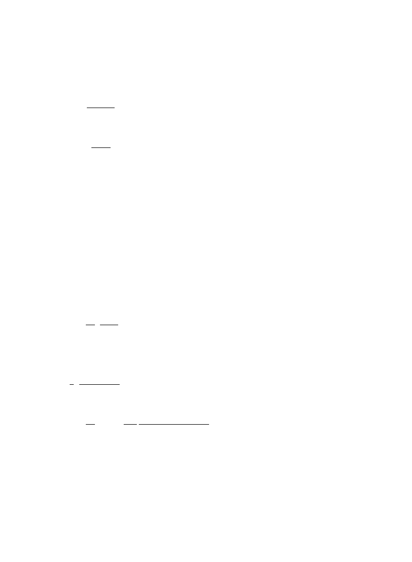
where

a)"

a2/2,

a52,

a!1)

a42 .

(4.125)

Thus, the minimum of Su corresponds to a"2, yielding

P(P2)&

SP2T

~bpg@2

(4.126)

The upper border of validity of (4.126) is P2&PRMT

(¸/l)

2&1/l2.

For hard wall boundary conditions, the asymptotic behavior of P(P2) will be, however,

determined by con"gurations with a maximum located near the sample boundary. Assuming that
the sample has a smooth boundary with the single characteristic scale ¸ (for example, it is of the
circular form), we can get such a state from the rotationally invariant bulk state by putting its
center on the boundary and removing that half of the state which is outside of the sample. Such
a truncated state will have the twice larger IPR and twice smaller action compared to its parent
bulk state. Consequently, the asymptotics of the distribution function for a sample with a boundary
will be di!erent from (4.126) by an extra factor 1/2 in the exponent.

Using the Liouville theory description (3.93), one can generalize the above consideration to the

distribution P(Pq) of higher IPR's Pq (3.90) with q'2 [160]. We will assume that q is not too large,

2(2bpg, so that the average value SPqT is at the same time the typical value of Pq (see Section

3.3.2). Then in the region q

2/bpg[Pq/SPqT!1[1 the distribution has the exponential form (3.92).

At larger Pq the optimal con"guration is again of the form Dt2(r)D4.005),eh(

)"A/ra for r'lp;

minimizing the action, we "nd

a"q/4 and the distribution function

P(Pq)&

SPqT

~2bpg@q

(4.127)

This is valid for Pq(PRMT

(¸/l)

2; for still larger Pq the corresponding optimal #uctuation would

violate the condition of the applicability of the di!usion approximation

h@[1/l. Incorporating this

restriction (cf. similar situation for the distribution of relaxation times, Section 4.1.2) leads to

1
q

ln(Pq/PRMT

)

ln(¸/l)

(4.128)

and to the log-normal far asymptotics

P(Pq)&

exp

bpg

2[(Pq/PRMT

)(¸/l)

ln(¸/l)

(4.129)

for (¸/l)

2[Pq/PRMT

q [

(¸/l)

2q~2.

4.5. 3D systems

As we will see below, in the 3D case the states determining the asymptotics of the distribution

functions have just a local short-scale spike on top of a homogeneous background. In this sense, no

317

A.D. Mirlin / Physics Reports 326 (2000) 259}382

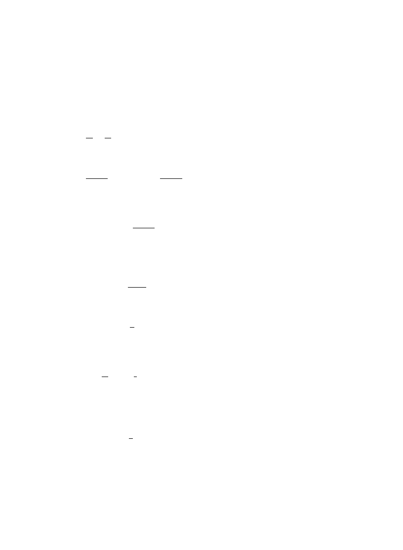
ALS is formed, in contrast to the quasi-1D and 2D situations. As a closely related feature, we "nd
that the results in 3D are strongly dependent on microscopic details of the random potential. We
start from discussing what the

p-model calculation gives when applied to the 3D geometry. Then

we compare this with the results of the direct optimal #uctuation method [161].

Let us consider, e.g. the long-time relaxation problem. The solution of the

p-model saddle-point

equation has the form [30]

h(r)KC

r4R ,

(4.130)

where R is the system size (which is, in fact, irrelevant here) and

l ln

q(kFl)2

;

C&ln

q(kFl)2

(4.131)

The reason for introduction of the short-scale cut-o! length l

H is the same as in 2D (see Sections

4.1.2 and 4.2.2): the gradient

h@ should not exceed &1/l. Calculating the action, we

"nd

ln Ps(t)&(kFl)2 ln3

q(kFl)2

(4.132)

with an uncertainty in numerical prefactor. This uncertainty originates from the fact that the action
is dominated by the ultraviolet (short-distance) region r&l

H . Similar result is obtained for the

eigenfunction amplitude statistics [33,36]

ln P(u)&(kFl)2ln3

(kFl)2

(4.133)

and for the LDOS distribution function [34]

ln P(

o)&(kFl)2ln3

(4.134)

As we see, all these distribution functions are found to have the exponential-log-cube asymptotic
form. The corresponding eigenstates have the shape

Dt2(r)D4.005)K

exp

2Zi

where Ci&1, Zt"t/[q(kFl)2], Zu"<u/(kFl)2, and Zo"o/l, i.e. they consist of the usual homo-

geneous background

Dt2(r)D4.005)"1/< supplemented by a short-scale bump containing only

a minor part of the eigenfunction normalization.

Muzykantskii and Khmelnitskii [31] applied the ballistic

p-model approach to the problem of

the long-time relaxation. They reproduced the result (4.132) and found the numerical prefactor
there to be equal to

p/9J3. On the other hand, Smolyarenko and Altshuler [161] employed

the direct optimal #uctuation method to study the asymptotics of the distribution function P(u).
This approach is similar to that used many years ago [162,163] to calculate the tails of the
density of states of a disordered system. The authors of [161] did not use the

p-model description,

but rather searched directly for the optimal realization of the random potential (hence their term

A.D. Mirlin / Physics Reports 326 (2000) 259}382

318

`direct optimal #uctuation methoda). While having con"rmed the exponential-log-cube form of the
asymptotics in the 3D case, they found a prefactor smaller by &kFl compared to the p-model

result, i.e. they obtained

P(u)&kFl ln3(u<) .

(4.135)

The physical reason for this di!erence lies in the ballistic e!ects which have been already

discussed in Section 3.3.3 in connection with perturbative corrections to the eigenfunction ampli-
tude distribution. It was shown there that in the 3D case and for the white-noise random potential
the parameter

i governing these corrections is dominated by a non-universal (depending on the

type of the disorder) ballistic contribution yielding

i&1/kFl, while the di!usive contribution is

1/(kFl)2. This is in direct correspondence with Eqs. (4.133) and (4.135), which show precisely the

same di!erence. Eq. (4.135) is again non-universal; its derivation by Smolyarenko and Altshuler
[161] relies on the white-noise disorder assumption. The corresponding optimal con"guration of
the potential found in [161] is nothing else but a potential wall surrounding the observation point
with the height several times larger than EF and the thickness &jF ln(u<). Such con"gurations are

not included in the

p-model consideration, which assumes that the absolute value of the particle

velocity does not change appreciably in space. If one would consider a smooth random potential,
whose magnitude is limited from above by some value ;.!9;EF, such con"gurations would not

be allowed. Whether in this case the

p-model result would hold remains to be seen.

4.6. Discussion

In Section 4, we have studied the asymptotic behavior of various distribution functions charac-

terizing the eigenfunction statistics in a disordered sample. For this purpose, we used two methods
of treatment of the

p-model: exact solution (in the quasi-1D case) and the saddle-point method.

Physically, the saddle-point solution describes the relevant optimum #uctuations of the wave
function envelope; probability of formation of such a #uctuation is found to be governed by the
Liouville theory (3.93). In the quasi-1D case, the results of the saddle-point method are in
agreement with those of the exact solution of the

p-model.

The 2D geometry is of special interest, since the eigenfunctions show the features of criticality. In

this case, a full agreement between the saddle-point calculation and the renormalization-group
(RG) treatment of Altshuler et al. [28] was found for all the distributions, where such a comparison
was possible, namely for P(t

(

), P(

o) and P(l). This agreement is highly non-trivial, for the

following reason. The RG treatment is based on a resummation of the perturbation theory
expansion and can be equally well performed within the replica (bosonic or fermionic) or
supersymmetric formalism. At the same time, the present approach based on the supersymmetric
formalism relies heavily on the topology of the saddle-point manifold combining non-compact (

j1)

and compact (

j2) degrees of freedom. The asymptotic behavior of the distribution functions

considered is determined by the region

j1<1 which is very far from the `perturbativea region of

the manifold QK

K (i.e. j1,j2K1). It is well known [164] that for the problem of energy level

correlation, the replica approach fails, since it does not re#ect properly the topology of the

p-model

manifold. The success of the RG treatment of [28] seems to be determined by the fact that for the
present problem (in contrast to that of level correlation) only the non-compact sector of the
supersymmetric

p-model is essential, with compact one playing an auxiliary role. Let us note that

319

A.D. Mirlin / Physics Reports 326 (2000) 259}382

the same situation appears in the vicinity of the Anderson transition [90,19,20] where the function
>

(

j1,j2) acquires a role of the order parameter function and depends on the non-compact variable

j1 only. The above agreement found for the `tailsa of the distributions in the metallic region

provides therefore support to the results concerning the Anderson transition obtained with making
use of the renormalization group approach and 2#

e expansion.

We have found that the spatial structure of ALS relevant to the asymptotic behavior of di!erent

distributions may be di!erent. This is because an ALS constitutes an optimal #uctuation for one of
the above quantities, and the form of this #uctuation depends on the speci"c characteristic, which is
to be optimized. Finally, we have discussed interrelations between asymptotics of various distribu-
tion functions. In the quasi-1D and 2D cases, we thus presented a comprehensive picture which
explains all the studied asymptotics as governed by exponentially rare events of formation of ALS.

5. Statistics of energy levels and eigenfunctions at the Anderson transition

In d'2 dimensions a disordered system undergoes, with increasing strength of the disorder,

a transition from the phase of extended states to that of localized states (see, e.g. [39] for review).
This transition changes drastically the statistics of energy levels and eigenfunctions. In particular,
at the mobility edge these statistics acquire distinct features re#ecting criticality of the theory. This
is the subject of the present section. Section 5.1 is devoted to the level statistics and Section 5.2
to the eigenfunctions correlations at the mobility edge. In Section 5.3 we study the level and
eigenfunction statistics in a quasi-one-dimensional model with long-range (power-law) hopping
which undergoes the Anderson transition and shows at criticality all the features characteristic for
a conventional metal-insulator transition point in d'2.

5.1. Level statistics. Level number variance

The problem of the energy level statistics at the mobility edge was addressed for the "rst time by

Altshuler et al. [40], who considered the variance

SdN2(E)T"SN2(E)T!SN(E)T2 of the number

of levels within a band of a width E. This quantity is related to the two-level correlator (2.1) via

SdN(E)2T"

WN(E)X

~WN(E)X

(

SN(E)T)!DsD)R(c)(s) ds ,

(5.1)

or, equivalently,

SN(E)T

SdN(E)2T"

WN(E)X

~WN(E)X

(c)(s) ds ,

(5.2)

where

SN(E)T"E/D and R(c)(s)"R(s)!1 is the connected part of the two-level correlation

function. In RMT, the 1/s

2 behavior of R(c)(s) leads to the logarithmic behavior of the variance

SdN2TWDK(2/p2b)lnSNT for SNT<1. In the opposite situation characteristic for the phase

of localized states, when all energy levels are completely uncorrelated (known as the Poisson
statistics), one gets

SdN2TP"SNT. Supported by their numerical simulations, Altshuler et al. [40]

A.D. Mirlin / Physics Reports 326 (2000) 259}382

320

put forward a conjecture that at the critical point

SdN2TKsSNT ,

(5.3)

where 0(

s(1 is a numerical coe

$cient (which is conventionally called now

`spectral compress-

ibility

a). More recently, Shklovskii et al. [41] introduced the concept of new universal statistics at

the mobility edge (see also Ref. [165]). In Ref. [42] the correlator R(s) at the mobility edge was
studied by means of perturbation theory combined with scaling assumptions about a form of the
di!usion propagator. It was found that for s<1,

(c)(s)Js~2`c

(5.4)

where

c(1 is certain critical index. The consideration of Ref. [42] led to the conclusion that

c"1!1/ld (where l is the critical exponent of the localization length), which was however
questioned later [166] in view of the oversimpli"ed treatment of the di!usion propagator at the
transition point in [42]. At any rate, the behavior (5.4) with some

c is what one expects to hold at

the mobility edge; the condition

c(1 follows from the requirement of convergence of :R(s) ds.

Using Eqs. (5.1) and (5.4) and the sum rule

R(s) ds"0

(5.5)

(implied by the conservation of the number of energy levels), the authors of [42] concluded that

SdN2TJNc

(5.6)

with

c(1, in contradiction with Ref. [40]. This conclusion was critically reexamined in Refs.

[43,44], where it was shown that the asymptotic behavior (5.4) of the correlator R(s) at s<1 does
not imply the absence of the linear term (5.3). The #aw in reasoning of Ref. [42] was in the
assumption that the universal part of the correlator R(s) (which is the one surviving in the limit
E/

D"SNT"const, ¸PR) satis

"es the sum rule (5.5). It turns out, however, that the sum rule is

ful"lled only if all contributions are taken into account, including the non-universal contribution of
the

`ballistica region u&1/q, where q is the elastic mean free time. To demonstrate this, we

estimate below (following Ref. [43]) the contributions to the sum rule from all regions of the
variable s.

In fact, for the conventional model of a particle in a random potential de"nition (2.1) of the

correlator and the sum rule relation (5.4) should be modi"ed, when the vicinity of the critical point
is considered. The reason is that the Anderson transition point corresponds to a strong disorder
regime EFq&1, so that the condition u&1/q implies u&EF. On the other hand, the density of

states

l(EF) can be considered as a constant only for small variations of energy u;EF. This means

that variation of

l(EF) should be taken into account in (2.1) and (5.5). Besides, the condition

EFq&1 leads to a breakdown of the perturbation theory, that complicates the analysis of the

`ballistica region contribution. To get rid of these problems, we consider a di!erent microscopic
model which has exactly the same universal part of R(s), but whose density of states does not change
within the range of

u&1/q. This is so-called n-orbital Wegner model [167], which can be

considered as a system of metallic granules forming a d-dimensional lattice, each granule being
coupled to its nearest neighbors. In the limit n<1 this model can be mapped onto a supersymmet-
ric

p-model de

"ned on a lattice. The action of this

p-model reads [90] (we consider the unitary

321

A.D. Mirlin / Physics Reports 326 (2000) 259}382

symmetry for de"niteness)

MQN"

WijX

Str QiQj#e+

Str QiK ,

(5.7)

where the supermatrices Qi are de"ned on sites i of a d-dimensional lattice with a lattice spacing a.

Summation in the "rst term of Eq. (5.7) goes over the pairs

SijT of nearest neighbors. The

parameters

C and e are related to the classical di

!usion constant D, the density of states

l, and the

frequency

u as follows:

C"plDad~2,

e"!iuplad/2 .

(5.8)

The two-level correlator can be expressed through a correlation function of this

p-model via the

discretized version of Eq. (2.10):

R(s)"Re

DQj

Str QikK

exp(!S

MQN) ,

(5.9)

where < is the system volume. It is not di$cult to prove explicitly [43] that the two-level
correlation function of this lattice

p-model, Eq. (5.9), satis

"es exactly the sum rule (5.5). As will

become clear below, the continuum version of the

p-model does not possess this property: there is

a de"ciency of the sum rule for it which is related with the contribution of the range of

u close to the

ultraviolet cut-o!.

Let us stress that in the region

u;D/a2,Ec(a) the correlator R(s) is universal, i.e. does not

depend on microscopical details of the model. The region

u&D/a2 plays a role analogous to that

of the ballistic region,

u&1/q, in the case of the usual model of particle in a random potential.

Despite the non-universality of the correlation function R/6(s) in this `ballistica domain, the

corresponding integral contribution I/6 to the sum rule is universal, because it determines,

according to Eq. (5.5), the sum rule de"ciency for the universal part R6(s):

I6#I/6"0 ,

I6"

(c)

(s) ds,

I/6"

(c)

(s) ds .

(5.10)

As will be seen below, when the system is close to the Anderson transition the two regions of the
variable s dominating the integrals I6 and I/6, respectively, are separated by a parametrically broad

range of s giving a negligible contribution to the sum rule. For energy band width E lying in this
range, we get from Eqs. (5.2) and (5.10)

SdN(E)2TKI6SN(E)T"!I/6SN(E)T ,

(5.11)

i.e. just the linear term (5.3) with

s"I6"!I/6. We turn now to the analysis of the correlator R(s)

and of the sum rule in various situation. For completeness, we start from the case of a good metal,
then we consider the critical point and the critical region cases.

(1) Good metal. Here the following three regions with di!erent behavior of R(s) can be found:
(A)

`Wigner}Dysona (WD) region: u;Ec. The correlator R(s) in this region was studied in

Section 2.2, see Eqs. (2.27) and (2.30). The corresponding contribution to the sum rule can be

A.D. Mirlin / Physics Reports 326 (2000) 259}382

322

estimated as (we omit numerical factors of order unity)

IAK

R(s)J#1/g .

(5.12)

(B)

`Altshuler}Shklovskiia (AS) region: Ec;u;Ec(a). Here Ec(a)"D/a2 is the Thouless

energy at the scale of lattice spacing a, which plays a role of the ultraviolet cut-o! for the di!usion
theory. The level correlation function is given by Eq. (2.33), yielding

IBK

D@a

R(s) dsJg

~d@2

d@2~1

1/g(a) ,

(5.13)

where g(a)"g(a/¸)

d~2 is the conductance at the scale a. Note that for the case of a particle in

a random potential, the following substitutions should be done: aPl; Ec(a)PEc(l)"1/q;

1/g(a)P1/g(l)J(

eq)d~1.

(C)

`Ballistica region: uZEc(a). To "nd the correlator R(s) in this range, we can neglect in the

leading approximation the "rst term in Eq. (5.7), that gives

(c)(s)J!

d 1

(5.14)

ICK

D@a

(c)(s) dsJ!1/g(a) .

(5.15)

Contribution (5.12) to the sum rule is dominated by the region

u&D, whereas the contributions

(5.13) and (5.15) are dominated by a vicinity of the ultraviolet cut-o!

u&D/a2. In d"3 g<g(a),

and these non-universal contributions IB, IC are much larger (by absolute value) than IA, but they

should cancel each other according to the sum rule. The situation is more interesting in d"2,
where the contribution (2.33), (5.13) of the AS region is absent in view of special analytical
properties of the di!usion propagator [168,169,44]. In this case g(a)"g, so that the contributions
IA and IC are of the same order, in agreement with the sum rule which prescribes their sum to be

zero. We can identify then IA with I6 and IC with I/6 in Eq. (5.10), so that I6"!I/6J1/g.

According to Eq. (5.11), this leads to a linear behavior of the variance,

SdN2TJ(1/g)SNT,

Ec;E;D/a2 ,

(5.16)

but the corresponding coe$cient is of order 1/g;1. The numerical coe$cient in (5.16) can be
calculated using the explicit form of R

(c)(s), yielding

s,I6K

bpg

g<1 .

(5.17)

With an increase in disorder strength, the coupling constant

C in Eq. (5.7) decreases. When it

approaches a critical value

C#, corresponding to the metal}insulator transition, the correlation

length

m becomes large: m<a. Depending on the relation between m and the system size ¸, the

following two situations are to be distinguished.

323

A.D. Mirlin / Physics Reports 326 (2000) 259}382

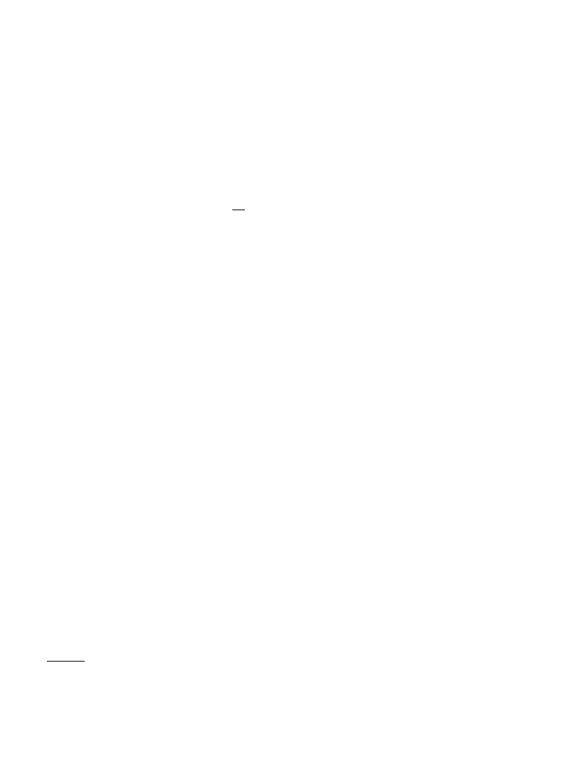
8 In 3D the value of g

H is, of course, of order unity. However, if one considers formally

d"2#

e with e;1, then

e is parametrically large. It is thus instructive to keep g

H as a parameter in all estimates.

(2) Metal in the critical region: a;

m;¸. In this case g(a)Kg

H , but

g,g(¸)<g

H , where

H is

the critical value of the conductance.

8 We

"nd then as much as four di!erent regions of s for the

correlator R(s):

(A) WD region:

u;Ec. The correlator R(s) and the contribution to the sum rule for this region

are given by the same Eqs. (2.27), (2.30) and (5.12), as for a good metal.

(B) AS region: Ec;u;Ec(m)"gHDm, where Ec(m) and Dm are Thouless energy and level spacing

for a piece of the sample with linear size

m. The correlator R(c)(s) is given by Eq. (2.33), and we

"nd

IBK

H D

(c)(s) dsJg~d@2g

d@2~1

1/g

H ,

(5.18)

where we have used the relations

Dm/D"(¸/m)d and g/gHJ(¸/m)d~2.

(C)

`Kravtsov}Lerner}Altshuler}Aronova (KLAA) region: Ec(m),gHDm;u;gHDa,Ec(a).

The correlator R

(c)(s) in this range was studied in Ref. [170]; the result reads:

(c)(s)K!g~c

H (D

D)1~cs~2`c

(5.19)

and, consequently,

ICK

H D

(c)(s) dsJ!1/g

(5.20)

(D)

`Ballistica region: uZEc(a). Here Eqs. (5.14) and (5.15) hold, yielding

IDJ!1/gH

(5.21)

The contribution IA is dominated by u&D, the contributions IB, IC by u&Dm, and "nally, the

contribution ID comes from the `non-universala region u&Ec(a). Therefore, this last contribution

determines I/6 in Eq. (5.10), leading according to Eq. (5.11) to the linear behavior of the variance

SdN2TJ(1/g

H )S

Ec(m);E;Ec(a)

(5.22)

with a coe$cient &1/g

H (which is of order unity in 3D).

(3) Finally, a system is at the critical point, when

m<¸. In this case, g(¸)"g(a)"g

H . The AS

region disappears, and we have, in full analogy with the previous estimates:

(A) WD region:

u[Ec"gHD.

IAJ#1/gH ,

(5.23)

(B) KLAA region: g

H D

;

u;DagH.

R(s)J!g

~2`c,

IBJ!1/gH ,

(5.24)

(C)

`Ballistica region: uZDagH.

ICJ!1/gH .

(5.25)

A.D. Mirlin / Physics Reports 326 (2000) 259}382

324

Again the same conclusion, as for the critical region case, can be drawn: the

`ballistica

contribution (5.25) can be identi"ed as I/6 in Eq. (5.10), yielding:

SdN2TKsSNT,

Ec;E;Ec(a) ,

(5.26)

with

s&1/g

H .

Recently, a relation between the spectral compressibility

s and the multifractal dimension D2 (for

discussion of multifractality and corresponding bibliographic references, see Sections 3.3.2 and 5.2)
was proposed [49,166]:

s"(d!D2)/2d .

(5.27)

The central idea of the derivation [49] is to consider the motion of energy levels, when the system is
subject to a random perturbation. This allows to link the spectral statistics with the wave function
correlations. In 2D, one can check, by comparing Eqs. (3.63) and (5.27), that Eq. (5.27) is indeed
satis"ed in leading order in 1/g. The general derivation of Eq. (5.27) is, however, based on certain
approximate decoupling of a higher-order correlation function [171,172,49], so that it is not
completely clear whether this is indeed an exact formula as argued in [49] or only an approxima-
tion valid for g

The linear behavior (5.3) of the level number variance at the Anderson transition has been

con"rmed by now in numerical simulations by several groups [45}48]. The spectral compressibil-
ity

s is an important universal parameter characterizing the critical point of Anderson transition.

Its universality is of the same sort as that of the critical indices, i.e.

s depends only on the spatial

dimensionality and on the symmetry (universality) class. Let us note that the whole level correla-
tion function R

(c)(s) is not as universal, since it depends also on the shape of the sample and on the

boundary conditions [48,173}175]. This can be expected already from the perturbative 1/g

correction, Eqs. (2.27) and (2.30), where the coe$cient ad does depend on the shape and on the

boundary conditions. Also, the shape dependence becomes evident if one considers the limit of an
elongated sample with a length considerably larger than the transverse sample size. Indeed, let us
consider (in 3D) a rectangular sample with ¸y"¸z"¸x/a, where a is a numerical factor [173]. If

we "x

a and consider the limit ¸PR, the level correlation function has a limiting form, which,

depends, however on

a. In particular, at a<1 the sample is of quasi-1D geometry with a ratio of

the sample length to the localization length &

a, so that the level statistics will be close to

Poissonnian.

Asymptotic behavior of the nearest-neighbor level spacing distribution function P(s) for s<1 at

the mobility edge has been also a controversial issue. We remind that for the Poissonnian statistics
P(s)"e

~s, while in the RMT P(s)&e~#0/45 s

. While Refs. [40,41] conjectured that P(s)&e

~#0/45 s,

the authors of Ref. [176] found P(s)&e

~#0/45 s

2~c

with the same index

c as in Eq. (5.4). Recent

numerical studies [177,178] support the former result, P(s)&e

~#0/45 s.

5.2. Strong correlations of eigenfunctions near the Anderson transition

In this section, we discuss correlations between the amplitudes of di!erent, but close in energy,

eigenstates at and near the critical point of the Anderson transition. Let us recall that in the metallic
phase far from the transition point a typical eigenfunction covers essentially uniformly the sample
volume. This is re#ected in the inverse participation ratio P2, as well as in the higher moments

325

A.D. Mirlin / Physics Reports 326 (2000) 259}382

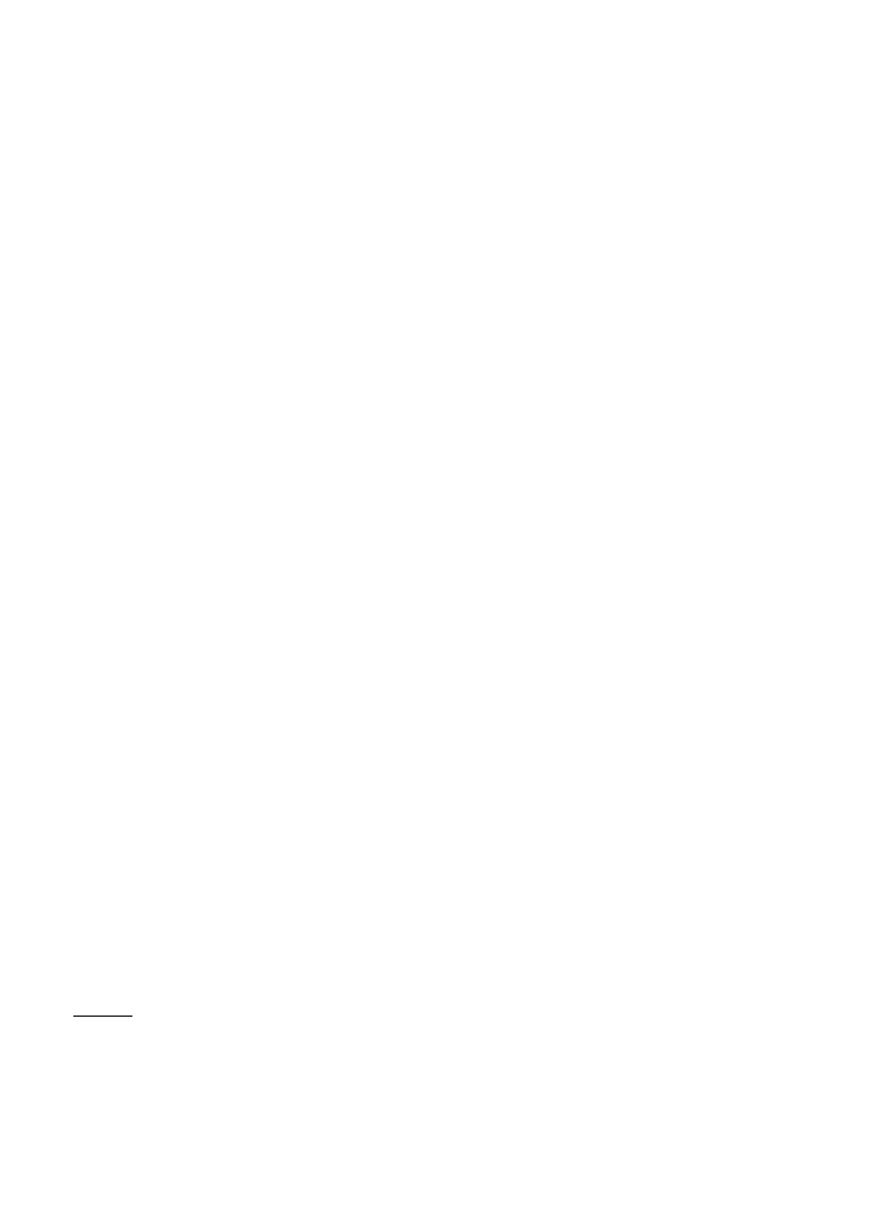
9 Eq. (5.30) was explicitly derived in [182] for the case of the sparse random matrix model [183,184] corresponding to

the limit of in"nite dimensionality, d"R. So, even at d"R, where the wave function sparsity (multifractality) takes its
extreme form, nearby in energy eigenfunctions are fully correlated.

Pq":ddr D t2q(r)D, which di!er only weakly from their RMT values, see Eqs. (3.15) and (3.52). When

the system approaches the point of the Anderson transition Ec, these extended eigenfunctions

become less and less homogeneous in space, showing regions with larger and smaller amplitudes
and eventually forming a multifractal structure in the vicinity of Ec, see Section 3.3.2. This

multifractal behavior is characterized by the following behavior of the moments Pq at the critical

point:

PqJ¸~D

(q~1), ¸(m ,

(5.28)

as well as in the conducting phase in the vicinity of the critical point:

PqJm(d~D

)(q~1)¸~d(q~1), ¸'m .

(5.29)

Here

mJDE!EcD~l is the correlation length and Dq is the set of multifractality exponents,

d'D2'D3'2. As Eq. (5.29) indicates, the eigenfunctions become more and more sparse when

the system approaches the critical point of the Anderson transition from the metallic phase (i.e.
when

m increases). Just at the mobility edge the scaling of IPR with the system size ¸ becomes

di!erent, see Eq. (5.28), so that the eigenfunction e!ectively occupies a vanishing fraction of the
system volume. At last, in the insulating phase any eigenstate is localized in a domain of "nite
extension

m, and IPR remains

"nite in the limit of in"nite system size ¸PR.

This transparent picture serves as a basis for qualitative understanding of spectral properties of

disordered conductors. Indeed, as long as eigenstates are well extended and cover the whole
sample, they overlap substantially, and corresponding energy levels repel each other almost in the
same way as in RMT. As a result, the Wigner}Dyson (WD) statistics describes well energy levels in
a good metal, see Section 2. In contrast, in the insulating phase di!erent eigenfunctions correspond-
ing to levels close in energy are localized far apart from one another and their overlap is negligible.
This is the reason for absence of correlations of energy levels in this regime, i.e. the Poisson
statistics.

A naive extrapolation of this argument to the vicinity of the transition point would lead to

a wrong conclusion. Indeed, one might expect that sparse (multifractal in the critical point)
eigenstates fail to overlap, that would result in essential weakening of level correlations close to the
mobility edge and vanishing level repulsion at E"Ec. However, numerical simulations show

[40,41,179}181] that even at the mobility edge levels repel each other strongly (although the level
statistics is di!erent from RMT). As we are going to explain now, this apparent contradiction is
resolved in the following way: The critical eigenstates for nearby levels are so strongly correlated
that they overlap well in spite of their sparse structure.

To demonstrate the strong correlations, we will consider the relation between the overlap

function

p(r, r, E, u), Eq. (3.68), and the `self-overlapa a(r, r, E), Eq. (3.67) (the latter determining the

IPR P2 according to P2":dra(r,r,E). As was shown9 in [182], everywhere in the metallic phase

A.D. Mirlin / Physics Reports 326 (2000) 259}382

326

(including the vicinity of the critical point)

p(r, r, E, u)"

b#2

a(r, r, E)

(5.30)

for

u;Dm, where Dm&1/lmd is the level spacing in the correlation volume. Eq. (5.30) implies the

following structure of eigenfunctions within an energy interval

u(Dm. Each eigenstate can be

represented as a product

Wi(r)"ti(r)UE(r). Here the function UE(r) is an eigenfunction envelope of

`humps and dipsa. It is the same for all eigenstates around energy E, re#ects the underlying gross
(multifractal) spatial structure, and governs the divergence of the inverse participation ratios Pq at

the critical point. In contrast,

ti(r) shows RMT-like #uctuations on the scale of the wave length. It

"lls the envelope function

UE(r) in an individual way for each eigenfunction, but is not critical, i.e. is

not sensitive to the vicinity of the Anderson transition. These Gaussian #uctuations are responsible
for the factor

b/(b#2) (which is the same as in the corresponding Gaussian Ensemble) in Eq. (5.30).

As was already mentioned, this picture is valid in the energy window

u&Dm around the energy

E; the number of levels in this window being large as

Dm/D&(¸/m)d<1 in the limit ¸<m. These

states form a kind of Gaussian Ensemble on a spatially non-uniform (multifractal for EPEc)

background

UE(r). Since the eigenfunction correlations are described by the formula (5.30), which

has exactly the same form as in the Gaussian Ensemble, it is not surprising that the level statistics
has the WD form everywhere in the extended phase [183,184]. For larger

u, p(r, r, E, u) is expected

to decrease as

u~g@d, where g"d!D2, according to the scaling arguments [131,185}189] (see

below), so that

p(r, r, E, u)/a(r, r, E)&(u/Dm)~g@d, u'Dm ,

(5.31)

up to a numerical coe$cient of order unity.

The above formulas are valid in the metallic regime, i.e. for ¸<

m. Exactly at the critical point

(

m<¸) they take the form

p(r, r, E, u)/a(r, r, E)&1, u(D

(5.32)

and

p(r, r, E, u)/a(r, r, E)&(u/D)~g@d, u'D .

(5.33)

Of course, Eq. (5.32) is not su$cient to ensure the WD statistics at the critical point, since there is
only of order of one level within its validity range

u&D. Indeed, the numerical simulations show

that the level statistics on the mobility edge is di!erent from the WD one [40,41,179}181].

However, Eq. (5.32) allows us to make an important conclusion concerning the behavior of R(s)

(or, which is essentially the same, of the nearest neighbor spacing distribution P(s)) at small
s"

u/D. For this purpose, it is su

$cient to consider only two neighboring levels. Let their energy

di!erence be

u0&D. Let us now perturb the system by a random potential <(r) with S<(r)T"0,

S<(r)<(r@)T"Cd(r!r@). For the two-level system it reduces to a 2]2 matrix M<ijN, i,j"1,2, with

elements <ij":ddr <(r)WHi(r)Wj(r). The crucial point is that the variances of the diagonal and

o!-diagonal matrix elements are according to Eq. (5.32) equal to each other up to a factor of order
of unity:

S<211T/SD<212DT"p(r,r,E,u)/a(r,r,E)&1 .

(5.34)

327

A.D. Mirlin / Physics Reports 326 (2000) 259}382

The distance between the perturbed levels is given by

u"[(<11!<22#u0)2#D<12D2]1@2.

Choosing the amplitude of the potential in such a way that the typical energy shift <11&D and

using Eq. (5.34), we "nd

SD<12D2T&D. As a result, the probability density for the level separation

u is for u;D of the form dP&(u/D)b du/D, with some prefactor of order of unity. We thus
conclude that in the critical point

P(s)Kcbsb, s;1 ,

(5.35)

with a coe$cient cb of order of unity, in agreement with the numerical "ndings [41,179,181].
5.2.1. Spatial correlations at the mobility edge

Another question that one can ask concerning the wave function correlations at the mobility

edge is how the correlations decay with distance in real space. Let us consider correlations

a(r, r@, E)

of the eigenfunction amplitudes in two di!erent points. Matching the behavior of

a(r, r@, E) at r"r@

with that at

Dr!r@D&minM¸, mN (where no strong correlations is expected), we

"nd in the metallic

phase (¸<

m<l)

a(r, r@, E)&¸~2dmg D r!r@D~g, l[Dr!r@D[m

(5.36)

and at the critical point (

m<¸)

a(r, r@, E)&¸~2d`gDr!r@D~g, l[Dr!r@D[¸ .

(5.37)

The same consideration can be straightforwardly applied to the higher correlation functions
SDt2q

(r)

DDt2q

@)DT, leading to the conclusion that they decay as

SDt2q

(r)

DDt2q

@)DTJDr!r@D~*d`q(q

)`q(q

)~q(q

)+ ,

where

q(q),(q!1)Dq has been already introduced in Section 3.3.2. These results were obtained

for the "rst time by Wegner [190] from renormalization-group calculations. The above formulas
for the spatial correlations at the mobility edge can be generalized to the correlator

p(r, r@, E, u)

of two di!erent eigenfunctions by using the scaling assumptions that this is the length

¸u"¸

(

D/u)1@d"(1/ul)1@d which will set the correlation range at

"nite

u. This give for the

correlations at criticality (l(

Dr!r@D(¸u(¸,m)

p(r, r@, E, u)&¸~2d(ul)~g@dDr!r@D~g .

(5.38)

Chalker and Daniell [185,186] conjectured that the di!usion propagator

c(r, r@, E, u), Eq. (3.77), has

the same behavior (5.38) at the mobility edge. Extensive numerical simulations [185,187}189] fully
con"rm this conjecture, which determines the form of the anomalous di!usion at the critical point
of the Anderson transition.

5.3. Power-law random banded matrix ensemble: Anderson transition in 1D

The ensemble of random banded matrices (RBM) is de"ned as the set of matrices with elements

Hij"Gija(Di!jD) ,

(5.39)

where the matrix G runs over the Gaussian ensemble, and a(r) is some function satisfying the
condition limr?= a(r)"0 and determining the shape of the band. In the most frequently considered

A.D. Mirlin / Physics Reports 326 (2000) 259}382

328

case of RBM the function a(r) is considered to be (exponentially) fast decaying when r exceeds some
typical value b called the bandwidth. Matrices of this sort were "rst introduced as an attempt to
describe an intermediate level statistics for Hamiltonian systems in a transitional regime between
complete integrability and fully developed chaos [191] and then appeared in various contexts
ranging from atomic physics (see [192] and references therein) to solid state physics [18] and
especially in the course of investigations of the quantum behavior of periodically driven Hamil-
tonian systems [193,194]. The most studied system of the latter type is the quantum kicked rotor
[104] characterized by the Hamiltonian

K "

K 2

(

m/~=

d(t!m¹) ,

(5.40)

where l

K "!i+ R/Rh is the angular momentum operator conjugated to the angle h. The constants

and I are the period of kicks and the moment of inertia, correspondingly, and <(

h) is usually

taken to be <(

h)"k cos h. Classically, the kicked rotor exhibits an unbound di

!usion in the

angular momentum space when the strength of kicks k exceeds some critical value. It was found,
however, that the quantum e!ects suppress the classical di!usion in close analogy with the
localization of a quantum particle by a random potential [104,195].

It is natural to consider the evolution (Floquet) operator ;

K that relates values of the wavefunc-

tion over one period of perturbation,

t(h, t#¹)";Kt(h, t), in the `unperturbeda basis of eigen-

functions of the operator

K : DlT"

p)1@2

exp(in

h), n"$0,$1,

2 .

The matrix elements

SmD;DnT tend to zero when Dm!nDPR. In the case <(h)"k cos h this decay

is faster than exponential when

Dm!nD exceeds b+k/+, whereas within the band of the e

!ective

width b matrix elements prove to be pseudorandom [104].

Let us note, however, that the exponentially rapid decay of

SmD;DnT in the above mentioned

situation is due to the in"nite di!erentiability of <(

h)"cos h. If we take a function <(h) having

a discontinuity in a derivative of some order, the corresponding matrix elements of the evolution
operator would decay in a power-law fashion in the limit

Dn!mDPR. In fact, there is an

interesting example of a periodically driven system where the matrix elements of the evolution
operator decay in a power-law way, namely the so-called Fermi accelerator [58]. The power-law
(pseudo-)random banded matrices appear also in other models of the quantum chaos, such as
a close-to-circular Bunimovich stadium [196}198] or a Coulomb center inside an integrable
billiard [59].

One may also consider the random matrix (5.39) as the Hamiltonian of a one-dimensional

tight-binding model with long-ranged o!-diagonal disorder (random hopping). A closely related
problem with non-random long-range hopping and diagonal disorder was studied numerically in
Ref. [199]. E!ect of weak long-range hopping on the localized states in a 3D Anderson insulator
was discussed by Levitov [200,201,324]. Similar models with a power-law hopping appear also in
other physical contexts [60}62,202].

As was shown in [18,102], the conventional RBM model can be mapped onto a 1D supermatrix

non-linear

p-model, which allows for an exact analytical solution. The same p-model was derived

329

A.D. Mirlin / Physics Reports 326 (2000) 259}382

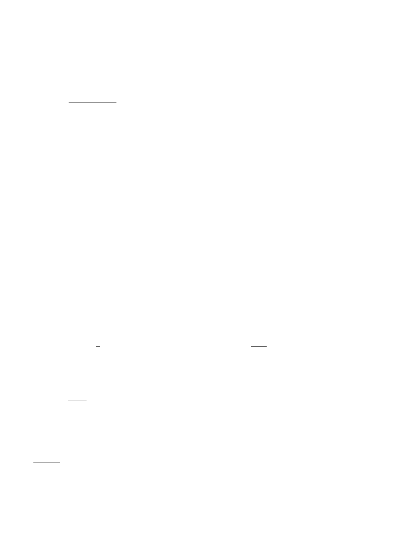
10 The expression for A0 is valid for a'1/2 and in the limit NPR. When a(1/2, A0 starts to have a dependence on

N which can be removed by a proper rescaling of the matrix elements Hij in Eq. (5.39). Then, the properties of the model

with

a(1/2 turn out to be equivalent to those of the GOE, so we will not consider this case any longer.

initially [6,101] for a particle moving in a quasi-1D system (a wire) and being subject to a random
potential. All states are found to be asymptotically localized, with the localization length

B2(2B0!E2)

2, Bk"

r/~=

2(r)rk .

(5.41)

However, for the case of a power-like shape of the band,

a(r)Jr

~a for large r ,

(5.42)

this derivation should be reconsidered. As explained below, this leads [57] to a more general 1D
p-model with long-range interaction, which is much richer than the conventional short-range one.
In particular, it exhibits the Anderson localization transition at

a"1. We mainly follow Ref. [57]

in our presentation.

5.3.1. Mapping onto the ewective

p-model

Let us consider the ensemble of large N

]N matrices (NPR) de

"ned

by Eq. (5.39) with

a function a(r) having the form

a(r)K

r(b ,

(r/b)

~a, r'b .

(5.43)

The parameter b will serve to label the critical models with

a"1. We will consider b to be large:

b<1, in order to justify formally the derivation of the

p-model. We will argue later on that our

conclusions are qualitatively valid for arbitrary b as well. We will call the ensemble (5.39), (5.43) the
power-law random banded matrix (PRBM) model. While considering localization properties, we
will restrict ourselves by one-loop calculation, and for this reason, by the orthogonal ensemble.

The PRBM model can be mapped onto the

p-model on a lattice,

MQN"!

1
4

(

plA0)2Str+

[(A

~1)ij!A~1

0 dij

]Q(i)Q(j)!

plu

Str Q(i)

K .

(5.44)

Here Q(i)"¹

i K

¹i satis"es the constraint

2(i)"1, A is the matrix with elements

Aij"a2(Di!jD), A0 is given by10 A0"+l Akl++=r/~= a2(r), and l is the density of states:

pA0

(4A0!E2)1@2 .

(5.45)

The standard next step is to restrict oneself to the long wavelength #uctuations of the Q-"eld. For

usual RBM characterized by a function a(r) decreasing faster than any power of r as rPR, this is

A.D. Mirlin / Physics Reports 326 (2000) 259}382

330

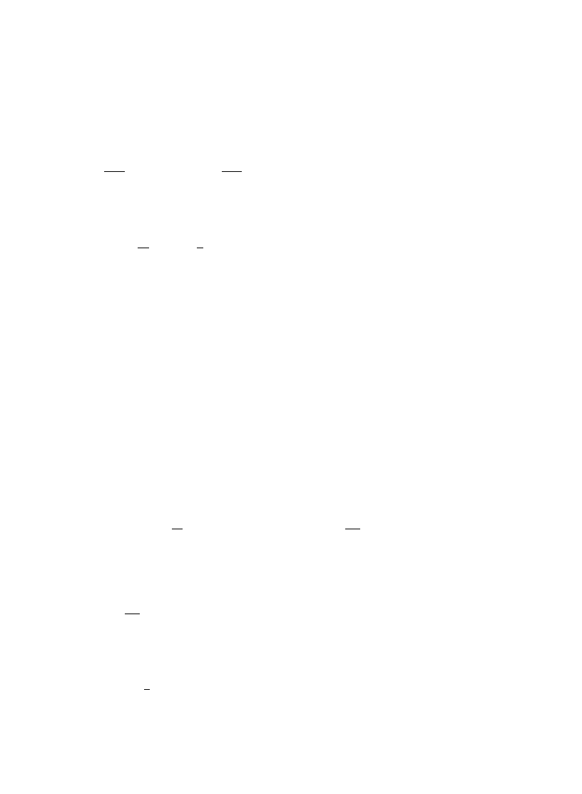
achieved by the momentum expansion of the "rst term in the action (5.44):

[(A

~1)ij!A~1

0 dij

]Q(i)Q(j),N

~1+

]QqQ~q

~1+

2QqQ~q"

dx(

RxQ)2 ,

(5.46)

where Qq is the Fourier transform of Q(i), and B2"+lAkl(k!l)2, as de"ned in Eq. (5.41). This

immediately leads to the standard continuous version of the non-linear

p-model:

MQN"!

Str

1
2

D0(RxQ)2#iuQK

(5.47)

with the classical di!usion constant D0"plB2, which implies the exponential localization of

eigenstates with the localization length

m"plD0Jb2.

Let us try to implement the same procedure for the present case of power-like bandshape (5.43).

Restricting ourselves to the lowest order term in the momentum expansion, we arrive again at
Eq. (5.47) as long as

a53/2. This suggests that for a53/2 the eigenstates of the present model

should be localized in the spatial domain of the extension

mJlD0. However, in contrast to the

usual RBM model this localization is power-like rather than exponential:

Dt(r)D2Jr~2a at r<m.

This is quite evident due to the possibility of direct hopping with the power-law amplitude. On
a more formal level the appearance of power-law tails of wave functions is a consequence of the
breakdown of the momentum expansion for the function A

in higher orders in q

2. The

presence of power-law

`tailsa of the wave functions, with an exponent a determined by the decay of

hopping elements, was found in numerical simulations in Refs. [197}199].

The most interesting region 1/2(

a(3/2 requires a separate consideration. In this case,

Eq. (5.46) loses its validity in view of the divergence of the coe$cient B2. We "nd instead

20(A~1

)+A0!Aq"2

dr a

2(r)(1!cos qr)

DqD

b@q@

dx(1!cos x)#(b

DqD)2a

b@q@

(1!cos x)

cab2aDqD2a~1 for 1/2(a(3/2 and DqD;1/b ,

(5.48)

where

ca"2

(1!cos x)

is a numerical constant, ca"[2C(2!2a)/(2a!1)]sin pa for aO1 and c1"p for a"1.

The corresponding long-wavelength part of the action,

S0MQN"!

Str

(dq)

DqD2a~1QqQ~q ,

(5.49)

331

A.D. Mirlin / Physics Reports 326 (2000) 259}382

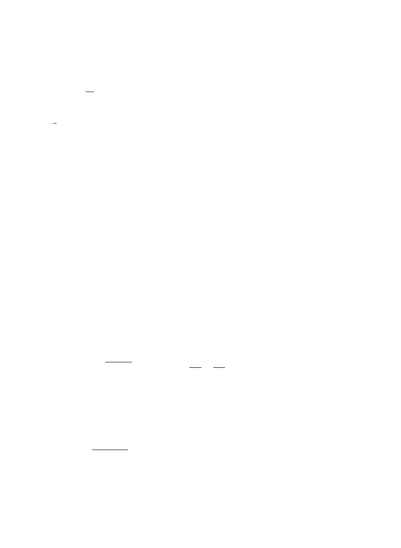
where

(dq),

dq
2

~1+

cannot be reduced to the local-in-space form in the coordinate representation any longer. Here,
1/t"

14(pl)2cab2aJb2a~1<1 plays the role of coupling constant, justifying the perturbative and

renormalization group treatment of the model described below.

Let us mention that if we consider the RBM model as a tight-binding Hamiltonian, the

corresponding classical motion described by the master equation on the 1D lattice is superdi!usive
for 1/2(

a(3/2 with a typical displacement in a time t being rJt1@(2a~1) (Levy law of index

a!1; see Ref. [203] for a review). As will be discussed in Section 5.3.3, this in

#uences the

asymptotic behavior of the spectral correlation function for the corresponding quantum system.

5.3.1.1. Perturbative treatment of the non-linear

p-model: General formulas. Here we derive one-

loop perturbative corrections to the density}density correlation function and inverse participation
ratios. Analysis of these expressions for various values of the power-law parameter

a will be

presented in Section 5.3.2.

The density}density correlation function (di!usion propagator)

K(r1,r2; u)"GE`u@2

(r1, r2)GE~u@2

(r2, r1)

can be expressed in terms of the

p-model as follows [6]:

K(r1,r2; u)"!(pl)2

DQQ12,ab(r1)kbbQ21,ba(r2)e~S

(5.50)

Here the indices p, p

@ of the matrix Qpp{,ab correspond to its advanced}retarded block structure,

whereas

a, b discriminate between bosonic and fermionic degrees of freedom. The matrix kbb is

equal to 1 for bosons and (!1) for fermions. To calculate the correlation function (5.50)
perturbatively, we use here the following parametrization [6] of the matrix Q:

K(=#J1#=2)"K

1#=#

(5.51)

where = is block-o!-diagonal in the advanced}retarded representation. To get the perturbative
expansion for K(r1, r2; u), one has to substitute Eq. (5.51) into (5.50), to separate the part quadratic

in = from the rest in the exponent and to apply the Wick theorem. In the usual case, when the
action is given by Eq. (5.47), the leading order (tree level) result reads in the momentum space as
follows:

K0(q, u)"

D0q2!iu

(5.52)

The perturbative quantum corrections do not modify the general form (5.52), but change the value
of the di!usion constant. In particular, in one-loop order one gets Eq. (5.52) with D0 replaced

A.D. Mirlin / Physics Reports 326 (2000) 259}382

332

by [204]

D"D0

pl<

/pn

D0q2!iu

(5.53)

This induces the standard weak-localization correction to the conductivity.

Now we implement an analogous procedure for the non-local

p-model of the type of Eqs. (5.44)

and (5.49):

MQN"

Str

r.r{

;

(r!r

@)Q(r)Q(r@)!i

Str

KQ(r) ,

(5.54)

with ;(r)Jr

~2a as rPR, so that the Fourier transform of ;(r) behaves at small momenta as

;

I (q)"!DqDp, 1/2(p(2 .

(5.55)

The exponent

p is related to the parameter a of the RBM model by p"2a!1. In leading order, we

keep in the action the terms quadratic in = only, which yields

K0(q, u)"

plt)~1DqDp!iu

(5.56)

corresponding to a superdi!usive behavior.

To calculate the one-loop correction to K0(q) (we set u"0 for simplicity) we expand the kinetic

term in S

MQN up to fourth order in =:

r,r{

Str ;(r!r

@)Q(r)Q(r@)D45) 03$%3"+

r,r{

1
4

Str =

2(r)=2(r@) .

(5.57)

The contraction rules are given by Eqs. (8) and (16) of Ref. [25] (reproduced below as Eq. (2.21) for
the unitary symmetry), with the propagator

P(q) replaced by

P(q)"t/8DqDp .

(5.58)

Evaluating the one-loop correction, we get the following expression for the density}density
correlation function up to the one-loop order:

~1(q)"K~1

(q)!

(

pl)2

(dk)

Dq#kDp!DkDp

DkDp

(5.59)

Now we calculate the perturbative correction to the inverse participation ratios Pq. The results

of Ref. [25] presented in Section 3.3.1 are straightforwardly applicable to the present case of
power-law RBM, provided the appropriate modi"cation of the di!usion propagator entering the
contraction rules is made, see the text preceding Eq. (5.58). One "nds

SPqT"

q(q!1)

P(r, r)

(2q!1)!!

q~1

(5.60)

where

P(r, r@)"(1/N)

(q)exp[iq(r!r

@)] and P(q) is given by Eq. (5.58).

333

A.D. Mirlin / Physics Reports 326 (2000) 259}382

11 Note that the =-

"eld renormalization is absent due to the supersymmetric character of the problem, which is

physically related to the particle number conservation [6].

5.3.1.2. Renormalization group treatment.

The e!ective

p-model, Eq. (5.54), is actually of one-

dimensional nature. However, for the sake of generality, we "nd it convenient to consider it here to
be de"ned in d-dimensional space with arbitrary d. The form (5.56) of the generalized di!usion
propagator implies that d"

p plays the role of the logarithmic dimension for the problem. In the

vicinity of this critical value we can carry out a renormalization group (RG) treatment of the model,
following the procedure developed for general non-linear

p-models in [205

}208]. We begin by

expressing the action in terms of the renormalized coupling constant t"Z

tBkd~p, where tB is the

bare coupling constant, Z1 is the renormalization constant, and k~1 is the length scale governing

the renormalization:

kd~p

2tZ1

rr{

;

(

Dr!r@D) Str [!=(r)=(r@)#J1#=2(r) J1#=2(r@)]

plu

Str

J1#=2(r) .

(5.61)

Expanding the action in powers of =(r) and keeping terms up to 4th order, we get

S"S0#S1#O(=6) ,

S0"

kd~p

4tZ1

rr{

;

(

Dr!r@D) Str (=(r)!=(r@))2!

plu

Str =

2(r) ,

S1"

kd~p

8tZ1

rr{

;

(

Dr!r@D) Str =2(r)=2(r@)#

plu

Str =

4(r) .

(5.62)

We have restricted ourselves to 4th order terms, since they are su$cient for obtaining the
renormalized quadratic part of the action in one-loop order. The calculation yields, after the
cancelation of an

:(dk)Jd(0) term with the contribution of the Jacobian:

S26!$"S0#SS1T

1
2

(dq) Str=q=~q

kd~p

tZ1

;

I (q)!

1
2

(dk)

;

I (k)!;I(k#q)

kd~p

tZ1

;

I (k)!

plu

(5.63)

According to the renormalization group idea, one has to chose the constant Z1(t)"1#at#2

so as to cancel the divergence in the coe$cient in front of the leading

DqDp term.

5.3.2. Localization and eigenfunction statistics

In this subsection we analyze the model in di!erent regions of the exponent

p"2a!1 using the

general formulas derived in Section 5.3.2.

A.D. Mirlin / Physics Reports 326 (2000) 259}382

334

5.3.2.1. Localized regime: 1(

p(2 (1(a(3/2). To evaluate the one-loop correction (5.59) to

the di!usion propagator, we use the expansion

Dq#kDp

DkDp

p
2

q;k ,

DqDp
DkDp

q<k .

(5.64)

Thus, the integral in Eq. (5.59) can be estimated as

(dk)

Dq#kDp

DkDp

k;q

(dk)

p!2

k:q

(dk)

DqDp
DkDp

(5.65)

and we are interested in the particular case of the dimension d"1. For

p'd"1 the integral

diverges at low k, and the second term in Eq. (5.65) dominates. This gives

I&¸

p~1DqDp ,

(5.66)

where ¸ is the system size determining the infrared cut-o! (in the original RBM formulation it is
just the matrix size N). This leads to the following one-loop expression for the di!usion correlator

K(q)"

(

pl)2tI

DqDp

I ~1"t~1! const ¸p~1 .

(5.67)

Now we turn to the renormalization group analysis, as described in Section 5.3.1. In the one-loop

order, the expression for the renormalization constant Z1 is determined essentially by the same

integral I, Eq. (5.65), with the RG scale

k playing the role of the infrared cut-o

! (analogous to that

of the system size ¸ in Eq. (5.67)). This yields (in the minimal subtraction scheme):

Z1(t)"1!

p!1

O(t

2) ,

(5.68)

leading to the following relation between the bare and the renormalized coupling constant
analogous to Eq. (5.67):

k1~p,

1
2

p!1

k1~p .

(5.69)

From Eq. (5.68), we get the expression for the

b-function:

b(t)" R

R lnk

(1!

p)t

1#t

Rt lnZ1(t)

(

p!1)t!

O(t

3) .

(5.70)

Both Eqs. (5.67) and (5.70) show that the coupling constant t increases with the system size ¸ (resp.
scale

k), which is analogous to the behavior found in the conventional scaling theory of localization

in d(2 dimensions [167,209]. The RG #ow reaches the strong coupling regime t&1 at the scale
k&t1@(p~1)

. Remembering the relation of the bare coupling constant tB and the index p to the

335

A.D. Mirlin / Physics Reports 326 (2000) 259}382

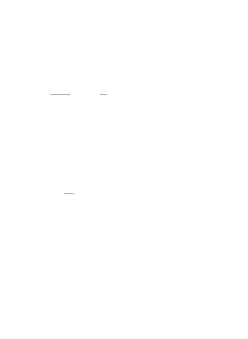
parameters of the original PRBM model: t

2a~1; pJ2a!1, we conclude that the length

scale

m&t~1@(p~1)

(2a~1)@(2a~2)

(5.71)

plays the role of the localization length for the PRBM model.

This conclusion is also supported by an inspection of the expression for the IPR, Eq. (5.60).

Evaluation of the one-loop perturbative correction in Eq. (5.60) yields

SPqT"

(2q!1)!!

q~1

1#q(q!1)

f(p)Np~1

(5.72)

where

f(p) is Riemann

's zeta-function;

f(p)K1/(p!1) for p close to unity. The correction term

becomes comparable to the leading (GOE) contribution for the system size N&t

1@(p~1), paramet-

rically coinciding with the localization length

m. For larger N the perturbative expression (5.72)

loses its validity, and the IPR is expected to saturate at a constant value

SPqT&m1~q for N<m.

In concluding this subsection, let us stress once more that the localized eigenstates in the present

model are expected to have integrable power-law tails:

Dt2(r)DJr~2a"r~p~1 at r<m.

5.3.2.2. Delocalized regime: 0(

p(1 (1/2(a(1). We begin again by considering the pertur-

bative corrections to the di!usion propagator (5.59). The "rst term in the r.h.s. of Eq. (5.65)
proportional to

:dk/k2 is determined by the vicinity of its lower cut-o

! (i.e. k&q), whereas the

second one is proportional to

:dk/kp and thus determined by the vicinity of its upper cut-o

(i.e. again k&q). Therefore, the integral (5.65) is now dominated by the region k&q, and is
proportional to

DqD. We get, therefore:

(

pl)2K~1(q)"

DqDp

CpDqD

(5.73)

with a numerical constant Cp.

We see that the correction term is of higher order in

DqD as compared to the leading one. Thus, it

does not lead to a renormalization of the coupling constant t. This is readily seen also in the
framework of the RG scheme, where the one-loop integral in Eq. (5.63) does not give rise to terms of
the form

DqDp. One can check that this feature is not speci

"c to the one-loop RG calculation, but

holds in higher orders as well. For the case of a vector model with long-ranged interaction this
conclusion was reached by Brezin et al. [210]. Thus, the renormalization constant Z1 is equal to

unity and the

b-function is trivial:

b(t)"(1!p)t .

(5.74)

This means that the model does not possess a critical point, and, for

p(1, all states are delocalized,

for any value of the bare coupling constant t. This property should be contrasted with the behavior
of a d-dimensional conductor described by the conventional local non-linear

p-model and under-

going an Anderson transition at some critical coupling t"t# [167].

Though all states of the model are delocalized, their statistical properties are di!erent from GOE.

In particular, calculating the variance of the inverse participation ratio P2 (see Section 3.3.3,

A.D. Mirlin / Physics Reports 326 (2000) 259}382

336

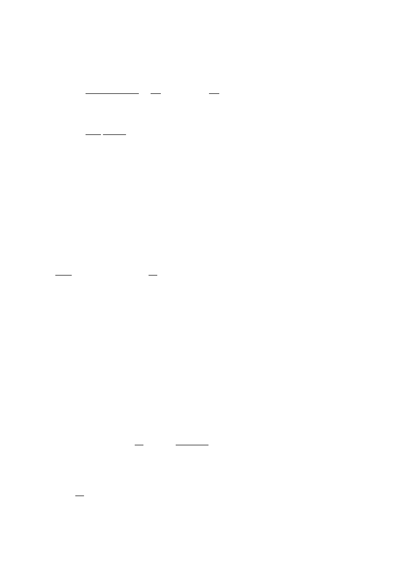
Eq. (3.89)) we get

d(P2)"

SP22T!SP2T2

SP2T2

rr{

P2(r, r@)"

q/pn@N_ n/1, 2,

P2(q) .

(5.75)

p'1/2 the sum over q is convergent yielding

d(P2)"

p2p

f(2p)

2~2p

(5.76)

Thus, in this regime the #uctuations of the IPR are much stronger than for the GOE where
d(P2)J1/N. Only for p(1/2 (a(3/4) the IPR #uctuations acquire the GOE character. Consid-

ering higher irreducible moments (cumulants) of the IPR,

|Pn2}, one "nds that the GOE behavior

is restored at

p(p(n)

1/n. In this sense, the model is analogous to a d-dimensional conductor at

d"2/

p. Therefore, only when pP0 (correspondingly, aP1/2 in the original PRBM formulation)

all statistical properties become equivalent to those characteristic of GOE.

5.3.2.3. Critical regime:

p"1 (a"1). As we have seen, p"1 separates the regions of localized

(

p'1) and extended (p(1) states. It is then natural to expect some critical properties showing up

just at

p"1. Let us again consider the generalized di

!usion propagator, Eq. (5.59). At

p"1 the

one-loop correction yields

(

pl)2

~1(q)"4DqD

~1!

ln(

DqD¸)

(5.77)

As expected at the critical point, the correction to the coupling constant is of logarithmic nature.
However, Eq. (5.77) di!ers essentially from that typical for a 2D disordered conductor:

~1"t~1

ln(¸/l) ,

(5.78)

where the bare coupling constant tB corresponds to scale l. Comparing the two formulas, we see

that in Eq. (5.77) the mean free path l is replaced by the inverse momentum q

~1. Therefore, the

correction to the bare coupling constant is small for low momenta q&1/¸, and the correlator K(q)
is not renormalized. This implies the absence of eigenstate localization, in contrast to the 2D
di!usive conductor case, where Eq. (5.78) results in an exponentially large localization length
mJexp t~1

. On a more formal level, the absence of essential corrections to the low-q behavior of

K(q) is due to the fact that the region k'q does not give a logarithmic contribution. This is
intimately connected with the absence of t renormalization at

p(1.

To study in more details the structure of critical eigenfunctions, let us consider the set of IPR Pq.

The perturbative correction, Eq. (5.60), is evaluated at

p"1 as

SPqT"

1#q(q!1)

ln(N/b)

(2q!1)!!

q~1

(5.79)

where the microscopic scale b, Eq. (5.43), enters as the ultraviolet cut-o! for the

p-model, the role

usually played by the mean free path l. This formula is valid as long as the correction is small:

ln(N/b)

~1@2

337

A.D. Mirlin / Physics Reports 326 (2000) 259}382

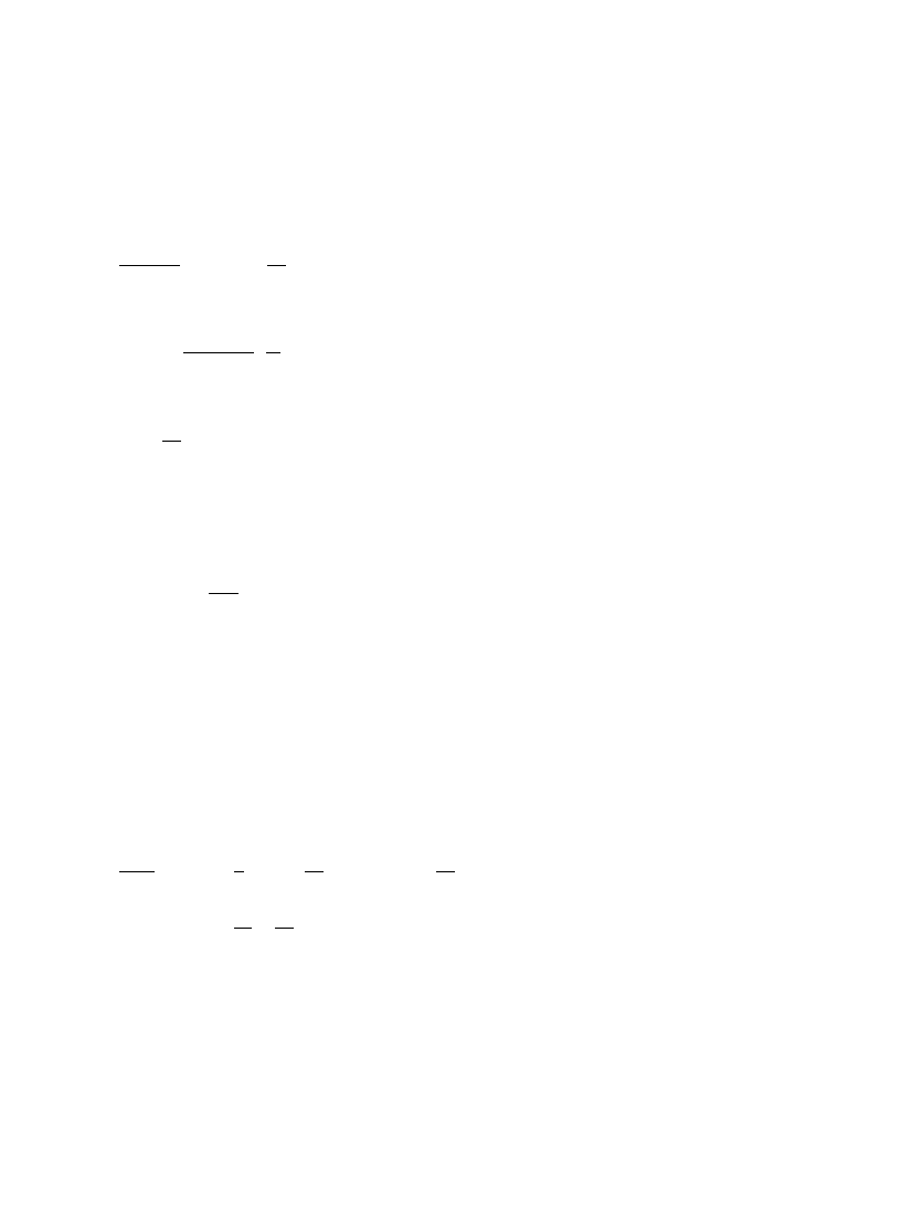
For larger q the perturbation theory breaks down, and one has to use the renormalization group
approach. This requires [28,50] introduction of higher vertices of the type zq:Strq(QkK)dr into the

action of the non-linear

p-model and their subsequent renormalization. The resulting RG equa-

tions for the charges zq read, in the one-loop order,

dzq

d ln

k~1

q(q!1)

zq ,

(5.80)

where

k~1 is the renormalization scale. Integrating Eq. (5.80), we

"nd

SPqT"

(2q!1)!!

q~1

q(q~1)t@8p

(5.81)

Note, that this formula is reduced to the perturbative expression, Eq. (5.79), in the regime

ln(N/b)

~1@2

The behavior described by Eq. (5.81) is characteristic of a multifractal structure of wave functions

(see Sections 3.3.2 and 5.2). Comparing (5.81) with (3.60), we "nd the multifractality dimensions
Dq"1!qt/8p. The general formula valid for both orthogonal (b"1) and unitary (b"2)

universality classes is

Dq"1!q

(5.82)

This form of the fractal dimensions is reminiscent of that found in two and 2#

e dimensions for the

usual di!usive conductor, see Eq. (3.63). The one-loop result (5.82) holds for q;8

p/t.

Now we can understand the reason for the q-dependent logarithmic correction to the di!usion

propagator K(q), Eq. (5.77). As was mentioned in the end of Section 5.2, the multifractality of
eigenfunctions determines the momentum dependence of the di!usion propagator at high q in the
critical point [185,186]

~1(q)JDqD(DqD¸)~g, g"d!D2

(5.83)

(at "nite frequency

u the system size ¸ is replaced by ¸u&(D/u)1@2). On the other hand, the

logarithmic correction in Eq. (5.77) is the "rst term of the expansion

(

pl)2

~1(q)"

DqD

ln(

DqD¸)#C2

ln(

DqD¸)

DqD

ln(

DqD¸)

(5.84)

where F(x) is some parameterless function. Since

g"1!D2Kt/4p, Eq. (5.84) has precisely the

form expected from (5.83), assuming that F(x)&e

~2x at x<1.

The set of fractal dimensions Dq (as well as spectral properties at p"1, see Section 5.3.3)

is parametrized by the coupling constant t. Strictly speaking, the above

p-model derivation is

justi"ed for t;1 (i.e. b<1). However, the opposite limiting case can be also studied, following
Levitov [200,201,324]. It corresponds to a d-dimensional Anderson insulator, perturbed by a weak

A.D. Mirlin / Physics Reports 326 (2000) 259}382

338

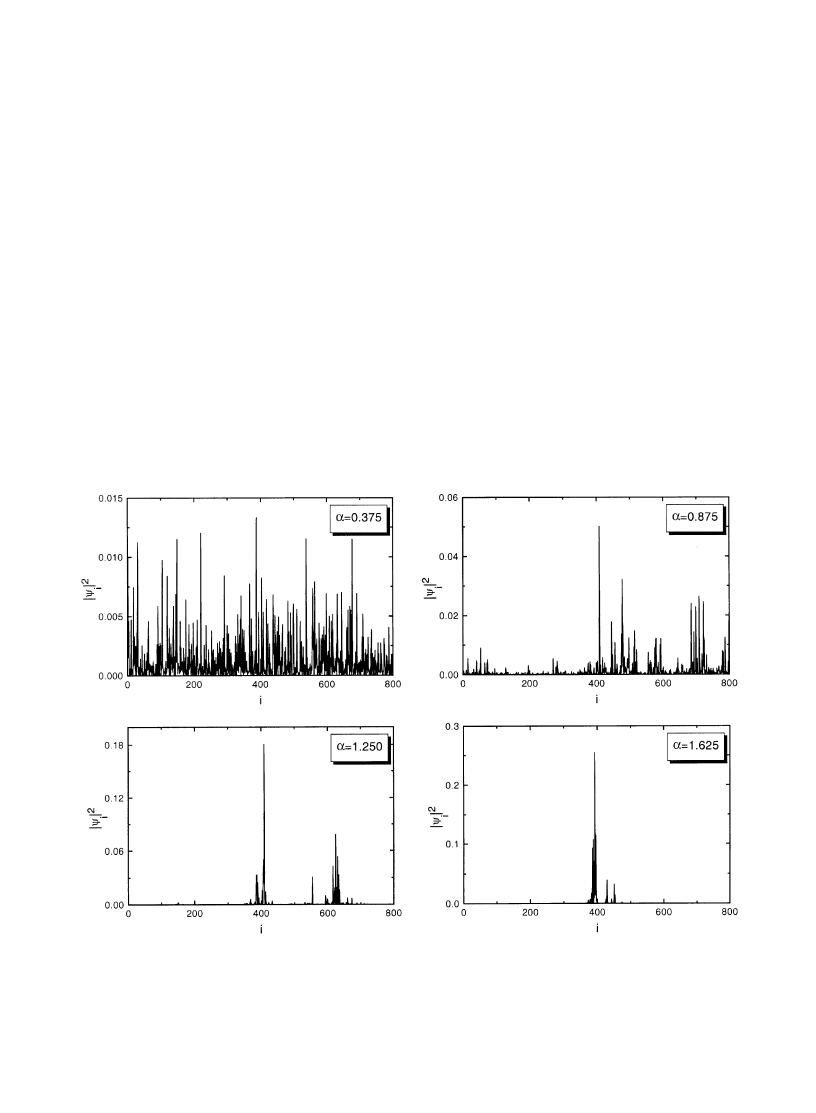
Fig. 3. Typical eigenfunctions for the matrix size N"800 and four di!erent values of

a: 0.375, 0.875, 1.250, and 1.625.

From [57].

long-range hopping with an amplitude decreasing with distance as r

~p. The arguments of Levitov

imply that the states delocalize at

p4d, carrying fractal properties at p"d. The PRBM model in

the limit b;1 is just the 1D version of this problem. This shows that the conclusion about
localization (delocalization) of eigenstates for

p'1 (resp. p(1), with p"1 being a critical point

holds irrespective of the particular value of the parameter b. The b;1 limit of the PRBM model
was also studied in Ref. [61] where the IPR P2 was calculated, yielding the fractal dimension

D2Jb. Alternatively, the regime of the Anderson insulator with weak power-law hopping can be

described in the framework of the non-linear

p-model, Eq. (5.54), by considering the limit t<1.

Formally, the non-linear

p-model for arbitrary t can be derived from a microscopic tight-binding

model by allowing n<1

`orbitalsa per site [167].

To summarize, the PRBM model (5.39), (5.43) with 0(b(R or the

p-model (5.54) with

a coupling constant 0(t(R represent at

p"1 a continuous family of critical theories

parametrized by the value of b (respectively, t).

5.3.2.4. Numerical simulations. Numerical simulations of the PRBM model were performed in
Ref. [57] for values of

a3[0,2] and b"1. In Fig. 3 we present typical eigenfunctions for four

339

A.D. Mirlin / Physics Reports 326 (2000) 259}382

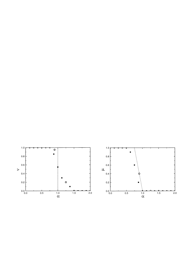
Fig. 4. Index

l characterizing the dependence of the inverse participation ratio SP2T on the matrix size N via

SP2TJ1/Nl, as a function of a. Points refer to the best-"t values obtained from matrix sizes between N"100 and

N"1000 (squares) or N"2400 (circles). The dashed line is the theoretical prediction for the transition from

l"1, at

small

a, to l"0, at large a. From [57].

Fig. 5. The same as Fig. 4, but for the index

k, derived from the N dependence of the variance d of the inverse

participation ratio:

d,(SP22T!SP2T2)/SP2T2J1/Nk. The dashed line corresponds to the predicted linear crossover

from

k"1 at a(3/4 to k"0 at a'1. From [57].

di!erent regions of

a. In agreement with the theoretical picture presented above, the eigenstates

corresponding to

a"0.375 and a"0.875 are extended, whereas those corresponding to a"1.25

and

a"1.625 are localized. At the same time, one can notice that the states with a"0.875 and

a"1.25 exhibit a quite sparse structure, as opposed to the other two cases. This can be explained
by the proximity of the former two values of

a to the critical value a"1.0 where eigenstates should

show the multifractal behavior. To get a quantitative information about the properties of the
eigenstates, the mean value of the IPR,

SP2T, and its relative variance, d"(SP22T!SP2T2)/SP2T2,

were calculated in [57]. At any given

a the dependences of the quantities SP2T and d on the matrix

size N were approximated by the power-laws

SP2TJ1/Nl, dJ1/Nk for N ranging from 100 to

2400. In Figs. 4 and 5 the values of the exponents

l and k obtained in this way are plotted versus the

PRBM parameter

a. The expected theoretical curves are presented as well. We see from Fig. 4 that

the data show a crossover from the behavior typical for extended states (

l"1) to that typical for

localized states (

l"0), centered approximately at the critical point a"1. The deviations from the

sharp step-like theoretical curve

l(a) can be presumably attributed to the

"nite-size e!ects which

are unusually pronounced in the PRBM model due to the long-range nature of the o!-diagonal
coupling. The data for the exponent

k (Fig. 5) also show a reasonable agreement with the expected

linear crossover,

k"4(1!a) for 3/4(a(1, see Eq. (5.76).

While the presented data are in good agreement with the above theoretical picture, a more

detailed numerical investigation of the structure of eigenstates and of spectral statistics is certainly
desirable. In particular, it would be especially interesting to study the critical manifold,

a"1,

where the multifractal properties of eigenstates and intermediate level statistics are predicted by the
theory.

A.D. Mirlin / Physics Reports 326 (2000) 259}382

340

5.3.3. Spectral properties

Let us consider now the spectral statistics of the PRBM model. In the

`metallica regime, the

leading correction to the Wigner}Dyson form RWD(s) of the level correlation function is given by

the properly modi"ed Eq. (2.30), i.e.

R(s)"

RWD(s) ,

(5.85)

where

rr{

P2(r, r@)"

q/pn@N_ n/1, 2,

P2(q)

p2p

2p~2,

p'1/2 ,

const

p2pb1~2p

~1, p(1/2 .

(5.86)

p(1/2 the sum divergent at high momenta is cut o

at q&

p/b; the procedure leaving

undetermined a constant of order of unity. The correlation function R(s) is close to its RMT value if
p(1 (the region of delocalized states), or else if p'1 and the system size N is much less than the
localization length

m, Eq. (5.71). Under these conditions, Eq. (5.85) holds as long as the correction

term is small compared to the leading one. This requirement produces the following restriction on
the frequency s"

u/D:

s(sc&

~1N1~p,

p'1/2 ,

~1b1@2~pN1@2J(Nb)1@2, p(1/2 .

(5.87)

At larger frequencies (s'sc), the form of the level correlation function changes from the 1/s2

behavior typical for RMT to a di!erent one, in full similarity with the Altshuler}Shklovskii regime
(2.33) in the case of a conventional d-dimensional conductor. Extending Eq. (2.28) to the present
case, we "nd

(c)(s)"

bp2

n/0,1,

plt

1~1@pt1@ps1@p~2,

p'1/2 (pO1) ,

2N~1b2p~1J(Nb)~1,

p(1/2 .

(5.88)

At last, let us consider the level statistics at criticality,

p"1. In this case the coe

$cient of

proportionality in the asymptotic expression (5.88) vanishes in view of analyticity:

(c)(s)&

p2b

(x!i

u)2

0 .

(5.89)

This is similar to what happens in the case of a 2D di!usive conductor (see Section 5.1). A more
accurate consideration requires taking into account the high-momentum cut-o! at q&b

~1. In full

341

A.D. Mirlin / Physics Reports 326 (2000) 259}382

analogy with the 2D situation mentioned we "nd then a linear term in the level number variance:

SdN2(E)TKsSN(E)T; s"

(c)(s) ds"

(5.90)

The presence of the linear term (5.90) (as well as the multifractality of eigenfunctions, Section 5.3.2)
makes the case

p"1 similar to the situation on the mobility edge of a disordered conductor in

d'2 discussed in Sections 5.1 and 5.2. Let us "nally mention that the value of

s, Eq. (5.90), is in

agreement with the formula (5.27), where D2 is given by Eq. (5.82) with q"2, and d"1 in the

present case. We stress, however, that both Eqs. (5.82) and (5.90) have been derived in the leading
order in t/8

p;1. As we discuss below, at t/8pZ1 Eq. (5.27) appears to be violated.

In fact, one can calculate the whole two-level correlation function using the results of Refs.

[10,11] presented in Section 2.2. We consider the unitary symmetry (

b"2) here for simplicity. In

this case, the level correlation function is described by a single formula R(s)"R1%35(s)#R04#(s)

[with R1%35(s) and R04#(s) given by Eqs. (2.38) and (2.34), respectively] in the whole range of s. The

spectral determinant D(s), Eq. (2.37) can be easily calculated [211], yielding

D(s)"

(

pst/16)2

sinh

2(pst/16)

(5.91)

in the case of periodic boundary conditions and

D(s)"

pst/8

sinh(

pst/8)

(5.92)

in the case of hard-wall boundary conditions. The resulting expressions for R(s) are

(c)(s)"!

sin

2ps

(

ps)2

(

pst/16)2

sinh

2(pst/16)

(5.93)

for periodic boundary conditions and

(c)(s)"!

p2s2

(

pst/8)2

sinh

2(pst/8)

2 cos(

ps)

pst/8

sinh(

pst/8)

(5.94)

for the hard-wall boundary conditions. Calculating the spectral compressibility

s":R(c)(s) ds, we

reproduce Eq. (5.90).

There exists a deep connection between the PRBM ensemble and the random matrix ensemble

introduced by Moshe et al. in Ref. [212]. This latter ensemble is determined by the probability
density

P(H)J

d; exp

M!Tr H2!h2N2 Tr([;, H][;, H]s)N ,

(5.95)

where

:d; denotes the integration over the group of unitary matrices with the Haar measure. The

parameter h allows to interpolate between the limits of the Wigner}Dyson (h"0) and the Poisson
(hPR) statistics. The relation between the ensemble (5.95) and the PRBM ensemble is established
as follows [211]. For any given unitary matrix ; the level statistics in the ensemble determined by
the density (5.95) (without integration over ;) is determined by the eigenvalues e

(k"1,2, N) of

A.D. Mirlin / Physics Reports 326 (2000) 259}382

342

;

. For N<1 a typical matrix ; has an essentially uniform density of eigenvalues, so that we can

consider as a typical representative the matrix with equidistant eigenvalues,

hk"2pk/N. Indeed,

weak #uctuations of

hk around these values do not a!ect essentially the behavior of a(r) in Eq. (5.97)

below. On the other hand, the matrices with strongly non-uniform density of eigenvalues represent
a vanishingly small fraction of the whole group volume and can be neglected. Making a trans-
formation to the eigenbasis of ;, we can transform P(H) to

P(H)Jexp

DHijD2

1#(2Nh)

2sin2

(i!j)

(5.96)

so that the matrix H has a form of the PRBM in the critical regime

a"1 with

2(r)"

b
4

sin

2(pr/N)

(

p/N)2

b
4

1#(r/b)

for r;N ,

(5.97)

and b"1/2

ph. Calculating (for h;1) the coupling constant in the center of the band (E"0)

according to Section 5.3.1, we get t"4/b"8

ph.

A nice feature of the ensemble (5.95) is that at

b"2 the level correlation function can be

calculated exactly for arbitrary value of h [212] (we remind that the above

p-model study of the

PRBM ensemble was restricted to the regime 1/2

pb"h;1). After the integration over the unitary

group with making use of the Itzykson}Zuber formula, the joint probability distribution of the
eigenvalues of H is found to be equal to the probability density of coordinates of a system of
non-interacting 1D fermions in a harmonic con"nement potential at "nite temperature. The
parameter h of the model (5.95) determines, in this formulation, the ratio of the temperature to the
Fermi energy, h"¹/EF, or, in other words, the degree of degeneracy of the Fermi gas. Calculating

the two-particle correlation function for non-interacting fermions, one "nds the sought level
correlation function [212]. In the center of the band the result reads

Sl(!u/2)l(u/2)T!Sl(0)T2"!

1#Ce

2*phNu

(5.98)

where C"[e

1@h!1]~1 and the mean level spacing D is given by

D~1"Sl(0)T"

1#Ce

(5.99)

The spectral compressibility

s is found from (5.98) and (5.99) to be

s"1!

:dp(1#Cep

)

:dp(1#Cep

)

(5.100)

343

A.D. Mirlin / Physics Reports 326 (2000) 259}382

The formulas (5.98) and (5.99) can be simpli"ed in the limits h;1 and h<1. For h;1, when the
gas is strongly degenerate, one gets (as usual, we introduce s"

u/D)

(c)(s)"!

sin

p2hs/2

sinh

p2hs/2

(5.101)

in precise agreement with the result (5.93) obtained directly for the PRBM ensemble (with the
above identi"cation of the parameters of the two models, t"8

ph).

In the opposite limit, h<1, the gas is almost classical and the correlations are weak,

(c)(s)"!e~2ph

(5.102)

Note that the corresponding spectral compressibility

sK1!1/J2h approaches unity in the limt

hPR, whereas the formula (5.27) would imply

s41/2. Therefore, at least for the PRBM model,

Eq. (5.27) is not an exact relation, but rather an approximation valid in the close-to-RMT regime
1/2

pb"h;1.

6. Conductance 6uctuations in quasi-one-dimensional wires

This section is devoted to a study of the conductance #uctuations of a quasi-one-dimensional

disordered system [64,65]. As was already mentioned in Section 3, there exist di!erent microscopic
models which can be mapped onto the same 1D supersymmetric

p-model and thus belong to

the same

`quasi-one-dimensional universality classa. Our treatment below will be based on the

Iida}WeidenmuKller}Zuk (IWZ) model [63] representing a wire as a sequence of coupled N

random matrices, the "rst and the last of which are coupled to the states propagating in the leads.
Using the multi-channel BuKttiker}Landauer formula [213}216], the mean conductance and its
variance can be expressed in terms of end-to-end correlation functions of the

p-model. Similarly to

what was done in Section 3.2, where the eigenfunction statistics was studied, these correlation
functions can be calculated exactly via the transfer-matrix method. This means that calculation of
the functional integral can be reduced to solution of a

`SchroKdinger equationa, which can be found

in terms of an expansion in corresponding eigenfunctions. The results depend on a single parameter

m (where ¸ is the sample length and m the localization length) and do not depend on details of the

underlying microscopic model. On top of the IWZ-model and two other models from the quasi-1D
class already discussed in Section 3.2 (the thick wire model of Efetov and Larkin and the random
banded matrix model), we mention here a system of weakly coupled 2D layers in strong magnetic

"eld [68,217}224]. In the quantum Hall regime the transport in each layer is due to edge states.

Tunneling between the layers leads to appearance of the transport in the transverse direction. The
coupled edge states propagating on a surface of the cylinder form a 2D chiral metal, which can be
described by a directed network model introduced by Chalker and Dohmen [217]. Mapping of this
problem onto the supersymmetric spin chain was done in [218,221]; further mapping onto the
supersymmetric

p-model was presented in [222]. If the number of layers is su

$ciently large, the

system is of quasi-one-dimensional nature. Very recent numerical study of the directed network
model [68] showed perfect agreement with the analytical results presented below. First experi-
mental realization of the multilayer quantum Hall system has been also reported recently [224].

A.D. Mirlin / Physics Reports 326 (2000) 259}382

344

6.1. Modeling a disordered wire and mapping onto 1D

p-model

The presentation below is based on Ref. [65]. We consider a quasi one-dimensional disordered

wire of length ¸, decomposed into K boxes with linear dimension l. With each box i (i"1,2, K)
we associate N electronic states

DikT (k"1,

2, N). The boxes 1 and K are coupled to ideal leads

i on the left (i"¸) and right (i"R) side of the disordered region. In each of these leads we have
a number of modes

DE, a, iT (a"1,

2) with transverse energy

ea whose longitudinal momentum

k is de"ned by their total energy E being equal to

ea#+2k2/(2mH%). Here mH% is the e!ective mass of

the electrons. We work at zero temperature. The Hamiltonian of the system reads

i,a

D E, a, iTE

E, a,

iD# +

i,j,k,l

Dik

ijklSjlD

i/1,K

k,a,i

dE(

DE, a, iT=iak(E,i)SikD#c.c.) .

(6.1)

The N

]N-matrices (Hiikl) are taken to be members of the Gaussian unitary (GUE), orthogonal

(GOE) or symplectic (GSE) ensemble. For de"niteness, we will consider the orthogonal symmetry
case in the present section; the results for all the three symmetry classes will be presented in
Section 6.2. In the GOE case, the elements H

iikl are independent real Gaussian random variables

with zero mean value and

SHiiklHiik{l{T"

(

dkl{dlk{#dkk{dll{) .

(6.2)

States in adjacent boxes are coupled by another set of Gaussian random variables with zero mean
values and

SHii`1

i`1i

lk T

2/N2.

(6.3)

All other matrix elements H

ijkl vanish. The coupling between channel and box states is e!ected by

the matrix elements =

iak(E,i). We assume that they do not depend on E and i, that they obey the

symmetry =

ika"=iHak"=iak and that they ful"ll the orthogonality relation

iak=ikb"dabx (i"1,K)

(6.4)

with x a normalization constant. Eq. (6.4) is convenient but does not result in any loss of generality
[8]. We note that =

iak vanishes unless i"1,K.

The conductance of the system is given by the many-channel Landauer}BuKttiker formula

[213}216],

(

DSRL

ab D2

DSLR

ba D2

)"2

DSRL

ab D2

(6.5)

The S-matrix S

ii{

of the IWZ-model reads [225]

ii{

dabdii{!2pi +

i,j,k,l

iak(i)(D~1)ijkl=jlb(i@) ,

(6.6)

345

A.D. Mirlin / Physics Reports 326 (2000) 259}382

where

ijkl"Edijdkl!Hijkl#iX1kldi1dj1#iXKkldiKdjK ,

(6.7)

Xikl"p

a/1

ika=ial (i"1,K) .

(6.8)

The S-matrix in Eq. (6.5) is taken at the Fermi energy E"EF, and N#) denotes the number of open

channels at this energy. It follows that in order to obtain

SgT and Sg2T we have to calculate the

ensemble average of a product of two resp.four propagators D

~1. Further manipulations are

completely analogous to those outlined in Section 2.1 for the case of the level correlation function.
We de"ne a supervector

t"(S11,S21,s1,sH1,S12,S22,s2,sH2) of real commuting (S) and complex

anticommuting (

s) variables, with the

"rst four components corresponding to the retarded and the

last four to the advanced sector. Then

~1)ijkl"

t](S11)jl(S11)ik exp

tsK1@2DKK1@2t

(6.9)

where D

K "diag(D, D, D, D, Ds, Ds, Ds, Ds), K"diag(1, 1, 1, 1,!1,!1,!1,!1). Products of two

and four propagators can be expressed in similar fashion (see Eq. (6.14) below). After averaging
of Eq. (6.9) over the Gaussian distribution of random variables entering D

K , we perform the

Hubbard}Stratonovitch transformation introducing 8

]8 supermatrices Ri (i"1,2,K) conju-

gate to the dyadic product

titsi and then take the large-N limit. As a result, the integration over

Ri is restricted to solutions of the saddle-point equation Ri"j2(E!Ri)~1, which have the form

j2!

K¹~1,p ) I!id ) Q ,

(6.10)

with Q"¹

K¹~1, Q2"1. As a result, Eq. (6.9) takes the form

S(D~1)ijklT"

D[Q]exp

d2v2

Str QiQi`1

]

t] (S11)jl(S11)ikexp

tsK1@2(EK#iXKK#idQK)K1@2t

S(S11)jl(S11)ikTQ .

(6.11)

Here (E

K )ijkl"Edkldij, (XK)ijkl"(X1)kldi1dj1#(XK)kldiKdjK and (QK)ijkl"dklQidij. The last line of

Eq. (6.11) introduces a short-hand notation

TQ.

According to Eqs. (6.5) and (6.6), the "rst two moments of the conductance are given by

SgT"8 +

klk{l{

X1ll{XKk{kS(D~1)K1

~1 s)1K

l{k{T

(6.12)

Sg2T"64

klk{l{oqo{q{

X1ll{XKk{kX1qq{XKo{oS(D~1)K1

~1s)1K

l{k{

~1)K1

~1s)1K

q{o{T

(6.13)

A.D. Mirlin / Physics Reports 326 (2000) 259}382

346

12 We use here a brief notation for the matrix elements of the Q-matrices. Each of the two upper indices runs from 1 to

8 according to ordering of components of a supervector introduced before Eq. (6.9).

The averages of products of the Green's functions relevant for

SgT and Sg2T can be expressed

similarly to Eq. (6.11) as follows:

S(D~1)K1

~1s)1K

l{k{T

S(S11)1l(S11)Kk(S12)Kk{(S12)1l{TQ ,

S(D~1)K1

~1 s)1K

l{k{

~1)K1

~1s)1K

q{o{T

S(S11)1l(S11)Kk(S12)Kk{(S12)1l{(S21)1q(S21)Ko(S22)Ko{(S22)1q{TQ .

(6.14)

For simplicity, we set E"0 below. Evaluating the contractions in (6.14), performing the convolu-
tion with the projectors

X1, XK in (6.12), (6.13) and using N#)<1, one comes after some algebraic

manipulations to the following

p-model representation12 of SgT and Sg2T [64,65]:

SgT"

I 2#)

D[Q]Q

exp

M!S[Q]N ,

(6.15)

Sg2T"

I 4#)

D[Q]Q

exp

M!S[Q]N ,

(6.16)

S[Q]"

Str QiQi`1#

I #)

Str

K(Q1#QK) .

(6.17)

Here N

I #)"N#)¹0, with ¹0"4dx/(d#x)2 being the so-called transmission coe$cient, and

m"(4v2/j2)l. In the weak-disorder limit, m<l, the discrete sum !(m/8l)

Str QiQi`1 can be

replaced by an integral

dz Str

(6.18)

which is precisely the continuous version of the 1D

p-model (see Sections 2 and 3) with m being the

localization length equal to

m"2plAD for a thick wire. The second term in Eq. (6.17) containing

Q1 and QK describes the coupling of the wire to the leads.

Let us note that the duplication of the number of "eld components in the supervector

t (which is

forced by the supersymmetric formulation) gave us enough #exibility to write down the expressions
Eq. (6.14) for products of two as well as of four propagators. As a result, we were able to express
both

SgT and Sg2T in terms of correlation functions of the usual `minimala p-model. We did not

have to introduce Q-matrices of larger dimension. This fact no longer holds true when higher
moments of the conductance are to be calculated. For that purpose we would have to introduce
supervectors of larger size to express higher-order products of propagators in a form analogous
to (6.14). The increase in the number of supervector components would force us to deal with
Q-matrices of larger dimension. This enlargement, while posing no di$culty to perturbative
calculations [28], gives rise to substantial complications in the case of the exact treatment.

347

A.D. Mirlin / Physics Reports 326 (2000) 259}382

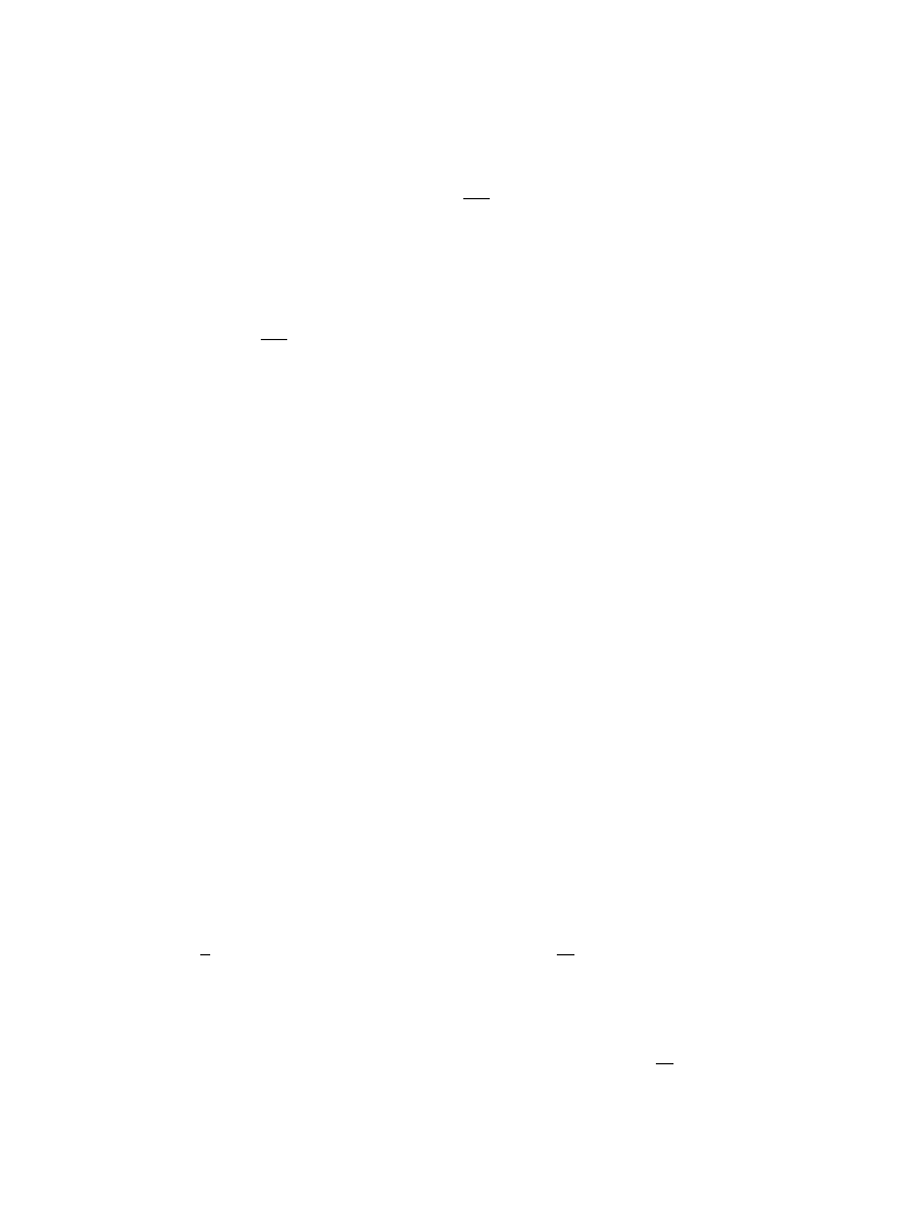
To introduce the transfer operator for the

`partition suma in Eq. (6.16), we de"ne the function

(QK, Q1;¸/2m)"

D[Q2]2D[QK~1]exp

32l

K~1

i/1

Str(Qi`1!Qi)2

(6.19)

which has the property

(QK`1, Q1; (¸#l)/2m)"

D[QK]=(QK`1, QK; l/2m)=(QK, Q1; ¸/2m)

D[QK]exp

32l

Str(QK`1!QK)2

(QK, Q1; ¸/2m) .

(6.20)

In the continuum limit

m<l, when Qi and Qi`1 are close to each other, one can reduce the integral

equation (6.20) to a di!erential one:

Rt="DQ= ,

(6.21)

lim
t?0

(Q, Q

@; t)"d(Q, Q@) ,

(6.22)

where

DQ is the Laplace operator on the non-linear space of Q-matrices. Eq. (6.21) has a form of the

heat (or di!usion) equation on this space, with = being the corresponding heat kernel.

6.2. Conductance yuctuations

Expressions (6.15) and (6.16) contain the e!ective number of open channels, N

I #), as a parameter.

As was shown in [63], the existence of this parameter sets an additional length scale ¸0"m/NI#).

For a very short system (¸;¸0), the conductance SgT is controlled by the sample-leads coupling

and is of order of N

I #). In this case, the zero-mode (i.e. spatially constant Q) approximation can be

used. We are interested here in the opposite limit ¸<¸0, where the resistance of the sample is

dominated by the bulk of the system. In this case, N

I #) becomes an irrelevant parameter and the

heat kernel itself already contains all information about

SgT and Sg2T. Since we assume that

I #)<1, the crossover length scale ¸0 is much less than m, so that the ratio of the sample length to

the localization length ¸/

m in the bulk-dominated regime can be arbitrary.

Using the generalized Fourier expansion of the heat kernel in the eigenfunctions of the Laplace

operator

DQ, one can "nd after very lengthy calculations [64,65] (there was a subtle error in the

GSE case in these papers corrected in [66]) the following exact results for

SgT and Sg2T for an

arbitrary value of the parameter ¸/

GOE:

SgnT(¸)"

p
2

j tanh2(pj/2)(j2#1)~1pn(1,j,j)exp

(1#

j2)

4 +

l|2

j1 dj2 l(l2!1)j1tanh(pj1/2)j2 tanh(pj2/2)

]pn(l,j1,j2) <

p,p

/B1

(!1#

pl#ip1j1#ip2j2)~1exp

2#j21#j22#1)

A.D. Mirlin / Physics Reports 326 (2000) 259}382

348

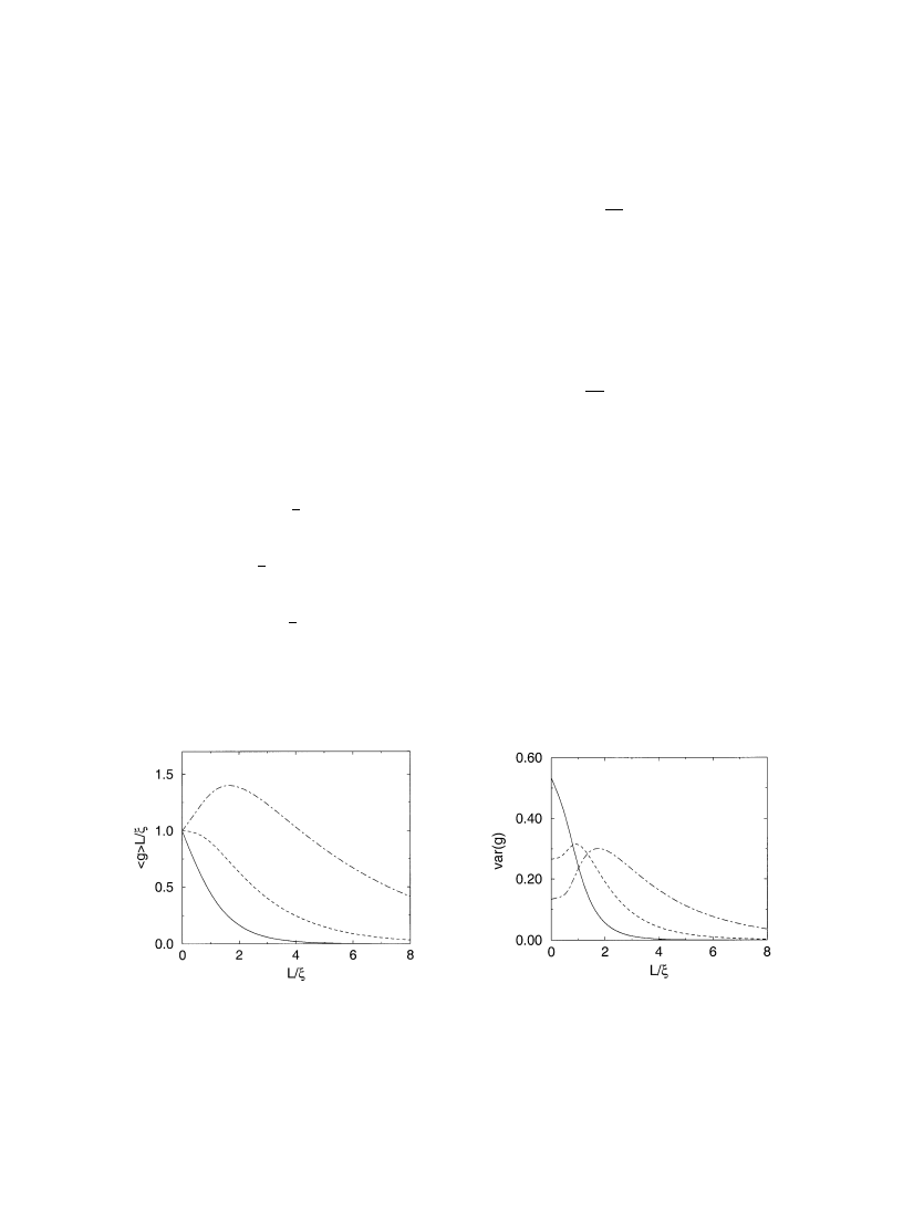
Fig. 6. Average conductance

SgT normalized to its Ohm

's law value as a function of the sample length (measured in units

m"2plAD). The full, dashed and dot-dashed lines correspond to the orthogonal, unitary, and symplectic symmetry,

respectively.

Fig. 7. The same as Fig. 6, but for the conductance variance var(g).

GUE:

SgnT(¸)"22 +

l|2

j j tanh(pj/2)l(j2#l2)~2pn(l,j)exp

2#j2)

(6.23)

GSE:

SgnT(¸)"25

j j(j2#1)tanh(pj/2)l1l2pn(j,l2,l2)

]

p,p

/B1

(!1#i

pj#p1l1#p2l2)~1exp

21#l22#j2!1)

The polynomials pn in the above expressions are given by

GOE:

p1(l, j1,j2)"l2#j21#j22#1 ,

p2(l, j1,j2)"12(j41#j42#2l4#3l2(j21#j22)#2l2!j21!j22!2) ,

GUE:

p1(l, j)"l2#j2,

p2(l, j)"12(l2#j2)2,

GSE:

p1(j, l1,l2)"j2#l21#l22!1 ,

p2(j, l1,l2)"14(l41#l42#2j4#3j2(l21#l22)!2j2#l21#l22!2) .

(6.24)

The results (6.23) are presented in Figs. 6 and 7 for all the three symmetry classes. The above

GUE formula is written for the case of broken time-reversal symmetry, but preserved spin-rotation

349

A.D. Mirlin / Physics Reports 326 (2000) 259}382

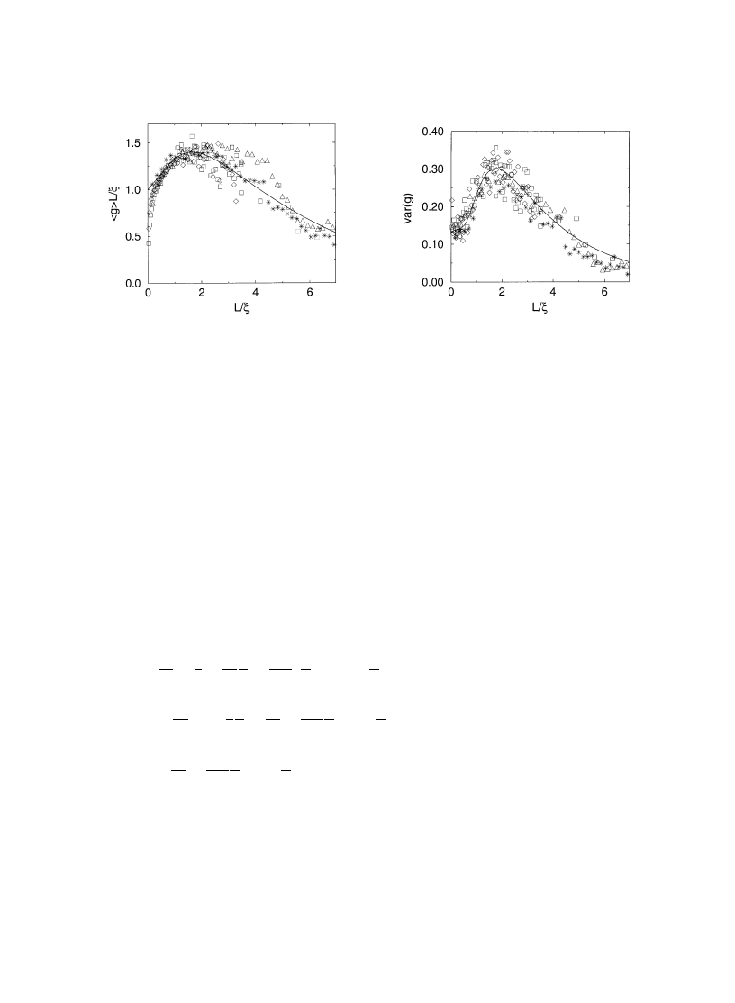
Fig. 8. Numerical data [67] for the average conductance in the case of symplectic symmetry. The box size N and the
number of channels N#) are equal to 10 (squares), 20 (diamonds), 60 (triangles), and 100 (stars). Each data point

corresponds to an average over 100 realizations of disorder. The full line is the theoretical prediction.

Fig. 9. The same as Fig. 8, but for the conductance variance.

invariance. The result for systems with broken time-reversal symmetry and with strong spin
interactions (e.g. systems with magnetic impurities, or systems with strong spin-orbit interaction in
magnetic "eld; to be denoted as GUE

@ below) is

SgnTGUE{(¸)"(1/2)nSgnTGUE(¸/2) .

(6.25)

The results (6.23) have been con"rmed by numerical simulations of the IWZ-model [67] and of the
directed network model [68]. In particular, we present in Figs. 8 and 9 the numerical results of [67]
for the symplectic symmetry class.

Let us discuss the behavior of Eqs. (6.23) in the limits of short (¸;

m) and long (¸<m) wire.

Condition ¸;

m corresponds to the metallic (weak localization) region, SgT<1. We

"nd in this

case the following perturbative (in ¸/

m) expansion for SgT, Sg2T and var(g):

SgT(¸)"

2
3

945

Sg2T(¸)"

8
3

52
45

136
945

(6.26)

var(g(¸))"

315

The perturbative results for the symplectic case are related to those for the orthogonal class via the
symmetry relations [226}228]

SgnTS1(¸)"(!1/2)nSgnTO(!¸/2) and have the form

SgT(¸)"

1
3

1890

A.D. Mirlin / Physics Reports 326 (2000) 259}382

350

Sg2T(¸)"

4
3

13
45

945

(6.27)

var(g(¸))"

315

Finally, for unitary symmetry we have

SgT(¸)"

Sg2T(¸)"

(6.28)

var(g(¸))"

The expressions for

SgT start from the Ohm

's law term 2

m/¸"4plAD/¸ (we remind that g is

measured in units of e

2/h"e2/2p+ and includes factor 2 due to the spin, while l is the density of

states per spin projection). The other terms constitute the weak-localization corrections. The
leading terms in var(g) are well-known values of the universal conductance #uctuations in the case
of quasi-1D geometry.

The opposite condition ¸<

m de

"nes

the region of strong localization. In this case, the

asymptotic behavior of

SgnT, n"1, 2, is as follows:

GOE:

SgnT"2~3@2~np7@2(m/¸)3@2e~L@2m ,

GUE:

SgnT"23~np3@2(m/¸)3@2e~L@4m ,

GSE:

SgnT"215@2~np3@2(m/¸)3@2e~L@8m .

(6.29)

Let us recall that

m is de

"ned here as

m"2plAD independently of the symmetry. The formulas

(6.29) demonstrate therefore well-known dependence of the localization length on the symmetry of
the ensemble, ¸-0#Jb. Let us stress, however, that in the GUE@ case (broken time-reversal and

spin-rotation symmetries), the results for which can be obtained via the relation (6.25) the
localization length is the same as in GSE [101,229]. This is because the transition GSEPGUE

not only changes

b from 4 to 2, but also breaks the Kramers degeneracy, increasing by factor of

2 the number of coupled channels. These two e!ects compensate each other. More generally,
localization length is proportional to

b/s, where s is the degeneracy factor.

6.2.1. DMPK equations

As has been already mentioned, calculation of higher moments

SgnT with n'2 and thus of the

whole distribution function P(g) has not been achieved in the supersymmetry approach because of
technical di$culties (necessity to increase the size of the Q-matrix with increasing n). The con-
ductance distribution in the localized regime ¸<

m can be approximately calculated from the

Dorokhov}Mello}Pereyra}Kumar (DMPK) approach. Within this approach, pioneered by
Dorokhov [230] and developed by Mello et al. [231], one derives a Fokker-Planck (di!usion)

351

A.D. Mirlin / Physics Reports 326 (2000) 259}382

equation for the distribution of transmission eigenvalues ¹n (the eigenvalues of the transmission-

matrix product tt

s). This equation is conveniently written in terms of the distribution function

j1,j2,2;¸), where ji"(1!¹i)/¹i and has the form

RP
R¸

n/1

Rjn

jn(1#jn)J

Rjn

~1P ,

i/1

j/i`1

Dji!jjDb ,

(6.30)

where l is the mean free path, N is the number of transverse modes, and

c"bN#2!b. Overview

of the results obtained within the DMPK approach can be found in the review article of Beenakker
[88]. It has been shown recently [66] that in the limit N<1 the DMPK approach is equivalent to
the supersymmetric

p-model considered above. Let us note that the DMPK approach is restricted

to calculation of transport properties of the quasi-1D conductor (which can be expressed through
the transmission eigenvalues ¹i), while the supersymmetry method allows to study all sorts of

quantities which can be expressed through the Green's functions (e.g. statistics of levels, eigenfunc-
tion amplitudes, local density of states etc. } see other sections of this article).

In the localized regime ¸<Nl the distribution function P(x1,2, xN;¸) with ji"sinh2xi (so

that ¹i"1/cosh2xi) takes the form [230,232,233]

P(x1,2, xl)"

p¸

N@2 N

n/1

exp

2¸

xn!

1;x1;x2;2;xn ,

(6.31)

where

mn"cl/(1#bn!b) are the inverse Lyapunov exponents. In the limit ¸PR all xn tend to

non-random values ¸/

mn, which is a manifestation of the Oseledec theorem (matrix generalization

of the

`law of large numbersa) [234}236]. For ¸/Nl<1 the conductance

g"G/(e

2/h)"2

n/1

¹n

(6.32)

is dominated by x1, e.g. gK2/cosh2x1K8e~2x

, which implies the Gaussian distribution of ln g,

P(ln g)K

p¸

1@2

exp

8¸

ln g#

2¸

(6.33)

with the average

Sln gT"!2¸/cl and the variance var(g)"4¸/cl"!2Sln gT. We have already

encountered the same log-normal distribution in Section 3.2.4, when we calculated the distribution
of the product of the wave function intensities in two points located close to the opposite edges of
the sample. The result (6.33) is fully con"rmed by numerical simulations as illustrated in Fig. 10.

The log-normal form (6.33) of the conductance distribution holds for g(1 only (since one

transmission eigenvalue cannot produce a conductance larger than unity); for g'1 the distribu-
tion P(g) decays very fast. The moments

SgnT with n51 are thus determined by the probability to

have g&1, which yields (with exponential accuracy)

SgnT&exp(!¸/2cl)

(6.34)

in full agreement with the asymptotics of the "rst two moments, Eqs. (6.29), found from the
supersymmetric approach. [Eqs. (6.29) contain also preexponential factors, for derivation

A.D. Mirlin / Physics Reports 326 (2000) 259}382

352

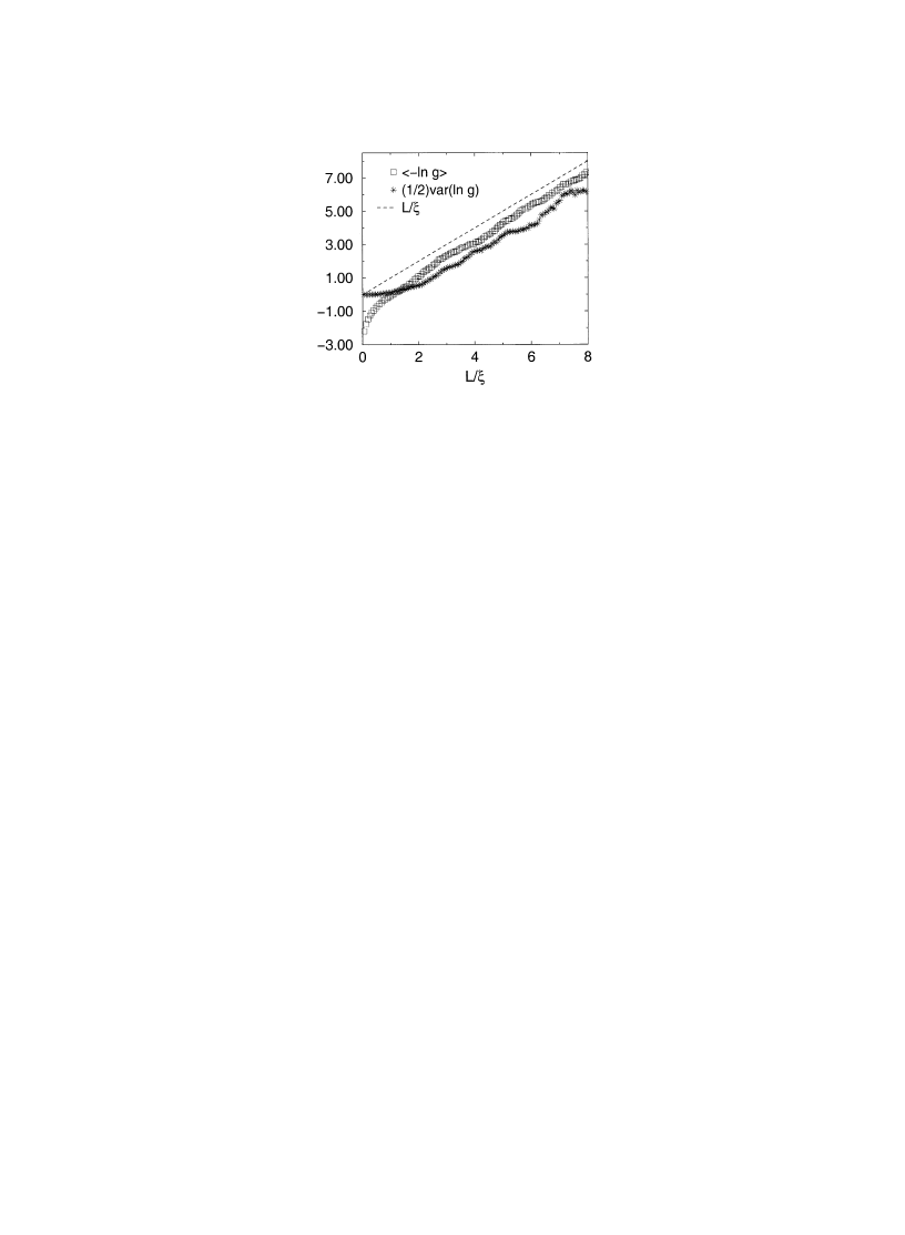
Fig. 10. The average and the variance of the conductance logarithm as a function of the sample length (for the symplectic
symmetry class). The box size N and the number of channels N#) are equal to 10. Each data point corresponds to an

average over 100 realizations of disorder. The dashed line corresponds to the formula (6.33).

of which the approximation (6.31), (6.33) of the solution of the DMPK equations is not
su$cient.]

Finally, we note that in the strictly 1D case Abrikosov [147] derived the exact result for the

conductance distribution function P(g) for arbitrary value of ¸/l. In the limit ¸/l<1 it approaches
the log-normal distribution (also found by Melnikov [145,146]), which can be obtained from
Eq. (6.33) by setting N"1 (i.e.

c"2). In fact, essentially equivalent results were obtained much

earlier in the context of the classical wave propagation, see Refs. [237}239].

7. Statistics of wave intensity in optics

As was already mentioned in the introduction, our statistical considerations are applicable not

only to properties of eigenfunctions and energy levels of quantum particles (electrons), but also to
those of intensities and eigenfrequencies of classical waves. This is related to similarity of the
stationary SchroKdinger equation and the wave equation. Propagation of the classical "eld

tu with

frequency

u in an inhomogeneous medium is described by the wave equation

[

+2#k20(1#k(r))]tu(r)"0 ,

(7.1)

supplemented by appropriate sources. Here k0"u/c, with c the speed of propagation in the

average medium, and

k(r) describes

#uctuations of the refraction index. The "eld

tu can describe

a component of the electromagnetic or acoustic wave. The impurity diagrammatic technique
[240}243] and the

p-model approach [244,245] can be developed in full analogy with the case of

the SchroKdinger equation in random potential.

Let us consider an open system with a permanently radiating source (for example, a point-like

source would correspond to addition of the term J

d(r!r0) in the r.h.s. of Eq. (7.1). The problem

of #uctuations of the wave intensity

t2u(r) in such a situation has a very long history. Almost

353

A.D. Mirlin / Physics Reports 326 (2000) 259}382

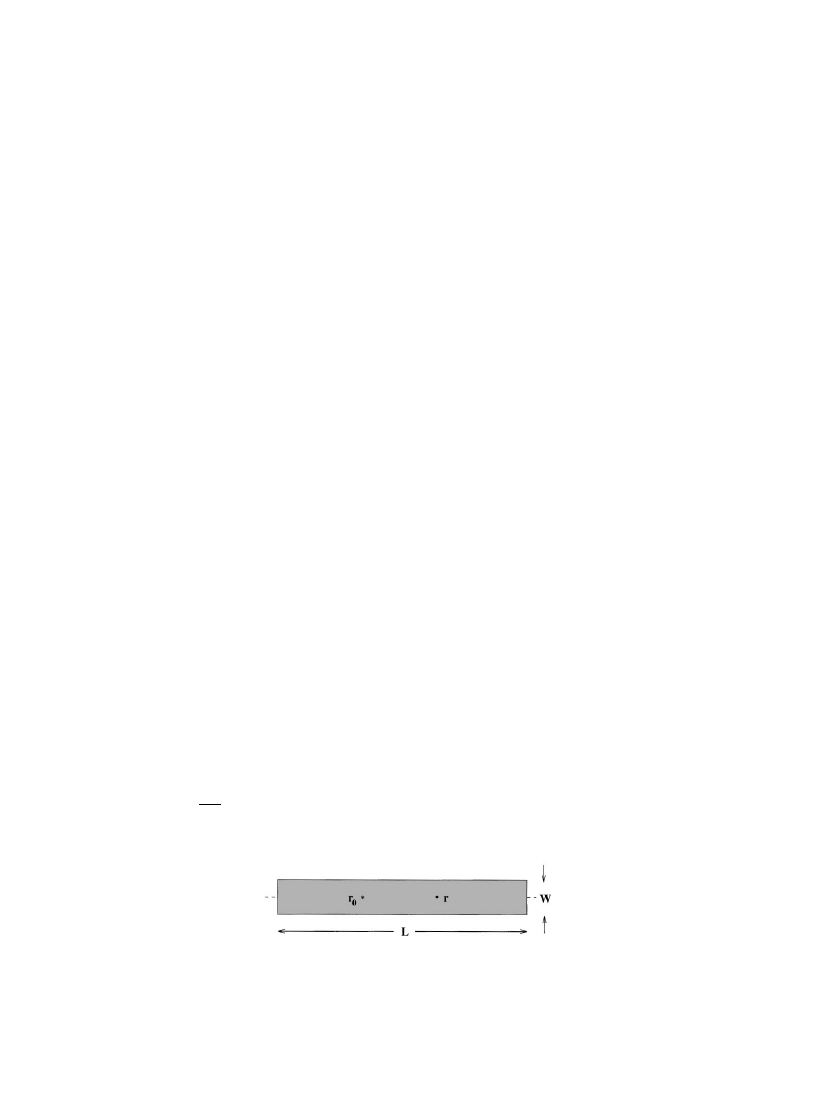
Fig. 11. Geometry of the problem. Points r0"(x0, y0, z0) and r"(x,y,z) are the positions of the source and of the

observation point (detector) respectively. From [71].

a century ago Rayleigh proposed a distribution which bears his name:

P0(II)"exp(!II) ,

(7.2)

where I

I is the intensity normalized to its average value, II"I/SIT. A simple statistical argument

leading to Eq. (7.2) is based on representing

tu(r) as a sum of many random contributions (plane

waves with random amplitudes and phases). This is essentially the same argument that was used by
Berry to describe #uctuations of eigenfunctions

ti in chaotic billiards and which leads to the RMT

statistics of

Dt2i(r)D (see Section 3). Let us mention, however, a di!erence between the two cases

(emphasized by Pnini and Shapiro [246]). In the case of an open system,

tu is a sum of traveling

waves, while for the closed system

ti is represented as a sum of standing waves. As a result, the

Rayleigh statistics has the same form as the statistics of eigenfunction amplitudes in a closed system
with broken time-reversal invariance (unitary class), where the eigenfunctions are complex.

Diagrammatic derivation of Eq. (7.2) is very simple [247] (see below); for the case of a smooth

randomness an essentially equivalent derivation [248] using path-integral arguments was given.
However, similarly to distributions of other quantities studied above (eigenfunction amplitude,
local DOS, relaxation time, etc.), distribution of optical intensities show deviations from the
Rayleigh law, which will be studied below. More speci"cally, we will consider #uctuations of the
intensity I(r, r0) at a point r induced by a point-like source at r0, with the both points r and

r0 located in the bulk of the sample. We will assume quasi-1D geometry of the sample with length

much larger than the transverse dimension = (see Fig. 11).
Let us note that there was a considerable activity recently in studying statistics of the transmis-

sion coe$cients ¹ab of a disordered waveguide [72}74,249,250]. In this formulation of the

problem, a source and a detector of the radiation are located outside the sample. The source
produces a plane wave injected in an incoming channel a, and the intensity in an outgoing channel
b is measured. The transmission coe$cients are related to the transmission matrix t (already
mentioned in Section 6) as ¹ab"DtabD2. One can also de"ne the transmittance ¹a"

¹ab

summed

over the outgoing channels. Finally, the total transmittance ¹"

a,b

¹ab

is the optical analogue of

the conductance g (#uctuations of which were studied in Section 6). Combining the diagrammatic
approach with the results on distribution of transmission eigenvalues in the metallic regime
(following from the DMPK equations), Nieuwenhuizen and van Rossum [72] calculated the
distribution functions P(¹a) and P(¹ab) for g<1. The results have the following form:

P(sa)"

~i=

exp[xsa!U#0/(x)] ;

(7.3)

A.D. Mirlin / Physics Reports 326 (2000) 259}382

354

P(sab)"

~i=

exp

sab

xv!

U#0/(x)

;

(7.4)

U#0/(x)"gln2(J1#x/g#Jx/g) ,

(7.5)

where sa"¹a/S¹aT and sab"¹ab/S¹abT. For large g<1 (i.e. in the `metallica regime), the

distribution P(sa), Eq. (7.3), has a Gaussian form,

P(sa)K

3g
4

exp

(sa!1)2

(7.6)

with log-normal tails at small sa;1 and an exponential asymptotics at large sa<1 of the form

P(sa)&exp(!gsa). The distribution of the channel-to-channel transmission coe$cients sab is

a close relative of the distribution of the point-to-point transmitted intensity I(r, r0) which was

discussed above and will be studied in detail below. For not too large sab it has the Rayleigh form,

P(sab)&e~s

, with the leading perturbative correction given by

P(sab)Ke~s

2ab!4sab#2)

sab;Jg

(7.7)

(this form of the correction to the Rayleigh law for the intensity distribution was found in a number
of papers, see Refs. [248,249,251,252]). In the intermediate region

Jg(sab(g Eq. (7.4) yields

P(sab)Kexp

sab

sab#2

(7.8)

(correction of this type was also obtained earlier, Refs. [252,253]). For large sab'g the distribution

acquires a stretched-exponential form

P(sab)&exp(!2Jgsab) .

(7.9)

We will return to Eq. (7.9) below, when comparing the results for the distribution of I(r0, r) with

P(sab). In the localized regime both distributions P(sa) and P(sab) are determined by the single

(largest) transmission eigenvalue and acquire the same log-normal form as the conductance
distribution, Eq. (6.33). We note also that van Langen et al. [74] were able to calculate P(sa) and

P(sab) in the case of the unitary symmetry, b"2, in the whole range of the parameter ¸/m (from

weak to strong localization). The distributions P(sa) and P(sab) were studied experimentally by

Garcia and Genack [254,255] and by Stoychev and Genack [256]; their "ndings are in good
agreement with the theoretical results.

Now we return to the statistics of the intensity I(r, r0). The "eld at the point r is given by the

(retarded) Green's function GR(r,r0) and the radiation intensity is I(r,r0)"DGR(r, r0)D2. The average

intensity

SI(r, r0)T is given diagrammatically by a di!uson ¹(r1,r2), attached to two external

vertices. The vertices are short-range objects and can be approximated by a

d-function times (l/4p),

so that

SI(r, r0)T"(l/4p)2¹(r,r0). For the quasi-one-dimensional geometry, the expression for the

di!uson reads

(r, r0)"

2 3

[z:(¸!z;)]

Al¸

(7.10)

355

A.D. Mirlin / Physics Reports 326 (2000) 259}382

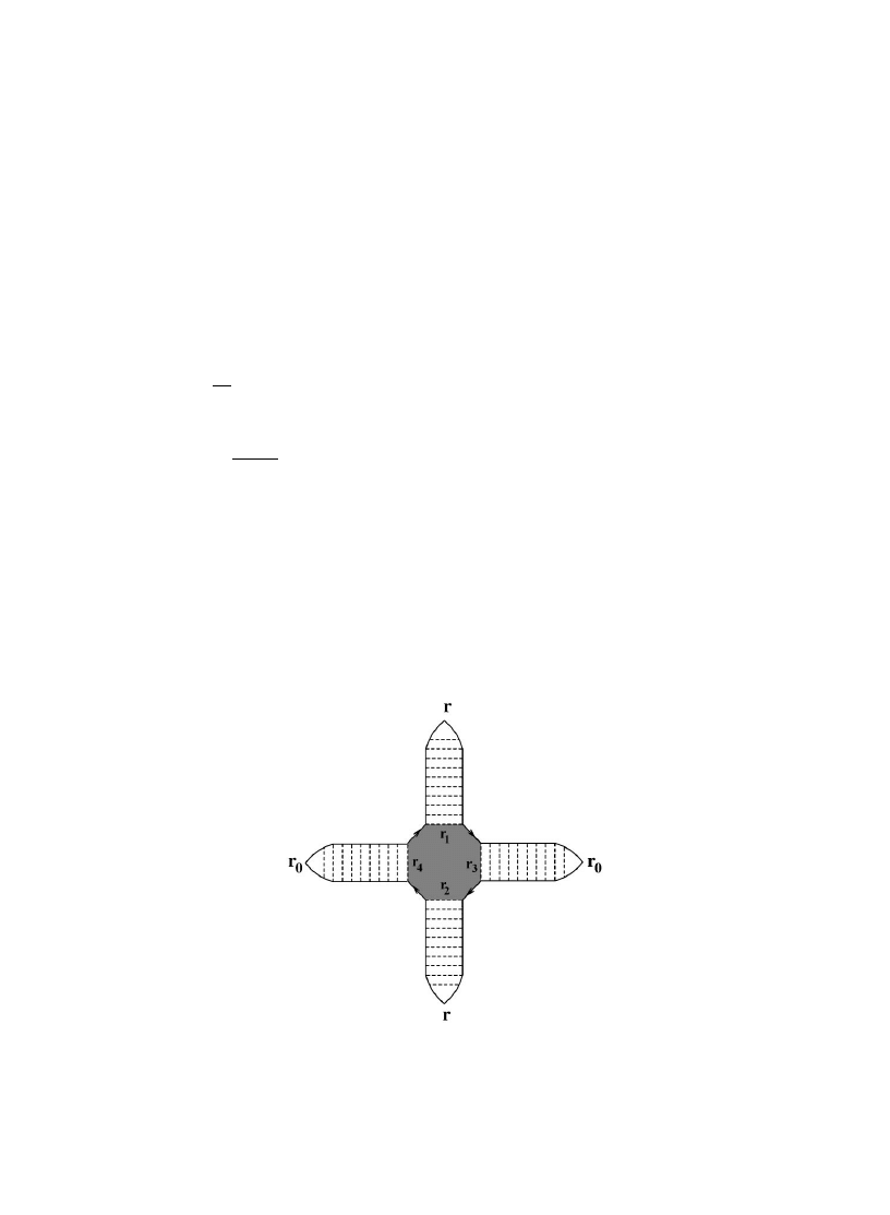
Fig. 12. Diagram for a pair of interacting di!usons. The external vertices contribute the factor (l/4

p)4. The shaded region

denotes the internal interaction vertex, see Eq. (7.11). From [71].

where l is the elastic mean free path, A is the cross-section of the tube, z-axis is directed along the
sample, z:"min(z,z0) and z;"max(z,z0). We assume that Dz!z0D<=.

The intensity distribution P(I) is obtained, in the diagrammatic approach, by calculating the

moments

SInT of the intensity. In the leading approximation [247], one should draw n retarded and

n advanced Green's functions and insert ladders between pairs

MGR,GAN in all possible ways. This

leads to

SInT"n!SITn and, thus, to Eq. (7.2).

Corrections to the Rayleigh result come from diagrams with intersecting ladders, which describe

interaction between di!usons. The leading correction is due to pairwise interactions. The diagram
in Fig. 12 represents a pair of

`collidinga di!usons. The algebraic expression for this diagram is

C(r, r0)"2

(r, r1)¹(r, r2)¹(r3, r0)¹(r4,r0)

]

pk20

3o[(+1#+2))(+3#+4)#2(+1 )+2)#2(+3 )+4)]

d(o!r

)

(7.11)

where k0 is the wave number and +

acts on r

. The factor (l/4

p)4 comes from the 4 external vertices

of the diagram, the ¹'s represent the two incoming and two outgoing di!usons and the expression
in the curly brackets corresponds to the internal (interaction) vertex (

`Hikami boxa) [257,258].

Finally, the factor 2 accounts for the two possibilities of inserting a pair of ladders between the
outgoing Green's functions. Integrating by parts and employing the quasi one-dimensional

A.D. Mirlin / Physics Reports 326 (2000) 259}382

356

geometry of the problem, we obtain (for z0(z):

C(z, z0)K2SI(z,z0)T2

(7.12)

where

SI(z, z0)T"

z0(¸!z)

Al¸

is the average intensity,

c"2g

2(3z#z0)!2¸z(z#z0)#2z20(z!z0)

1 ,

(7.13)

and g"k

20lA/3p¸<1 is the dimensionless conductance of the tube. For simplicity, we will assume

that the source and the detector are located relatively close to each other, so that

Dz!z0D;¸, in

which case Eq. (7.13) reduces to

c"g¸2/2z(¸!z). (All the results are found to be qualitatively the

same in the generic situation z0&z!z0&¸!z&¸.)

In order to calculate

SInT one has to compute a combinatorial factor which counts the number

Ni of diagrams with i pairs of interacting di!usons. This number is Ni"(n!)2/[22ii!(n!2i)!]K

(n!/i!)(n/2)

2i. For not too large n;c1@2 it is su

$cient to keep the i"1 contribution, yielding the

leading perturbative correction [71],

SIInT"n!

n(n!1)

(7.14)

or in terms of the distribution function,

P(I

I )"e~I

I 2!4II#2)

I ;c1@2.

(7.15)

For larger n (or, equivalently, I

I ) we have to sum up the series over i, yielding

SInT
SITn

*n@2+

1
i!

n! exp(2n

2/3c) .

(7.16)

Although i cannot exceed n/2, the sum in Eq. (7.16) can be extended to R, if the value of n is
restricted by the condition n;

c. Eq. (7.16) represents the leading exponential correction to the

Rayleigh distribution. Let us discuss now e!ect of higher order

`interactionsa of di!usons.

Diagrams with 3 intersecting di!usons will contribute a correction of n

3/c2 in the exponent of

Eq. (7.16), which is small compared to the leading correction in the whole region n;

c, but

becomes larger than unity for n

Zc2@3. Likewise, diagrams with 4 intersecting di

!usons produce

a n

4/c3 correction, etc. Restoring the distribution P(I), we

"nd [71]

P(I

I )Kexp

I #

I 2#O

I 3

(7.17)

Eqs. (7.14), (7.15) and (7.17) are analogous to those found in the case of transmission coe$cient
statistics, (7.7), (7.8), with the only di!erence that the parameter g is now replaced by

c/2 (if we

357

A.D. Mirlin / Physics Reports 326 (2000) 259}382

consider the limit z0P0, zP¸, then cP2g, so that both results are consistent). As has been

already mentioned, deviations of this form from the Rayleigh distribution of intensities were found
earlier by various authors [248,249,251}253]; a value of the parameter governing the strength of
deviations (here 1/

c) depends, however, on the geometry of the problem. It should be realized that

Eq. (7.17) is applicable only for I

I ;c&g and, thus, does not determine the far asymptotics of P(I).

The latter is unaccessible by the perturbative diagram technique and is handled below by the
supersymmetry method.

For technical simplicity, we will assume now that the time reversal symmetry is broken by some

magnetooptical e!ects (unitary ensemble). The moments of the intensity at point r due to the source
at r0 are given by

SInT"

[DQ](Q12,bb(z))n(Q21,bb(z0))ne~S*Q+ ,

(7.18)

where S[Q] is the zero-frequency

p-model action,

S[Q]"!

plD

3r Str(+Q)2 ,

(7.19)

which reduces in the quasi-1D geometry to

S[Q]"!(g¸/8)

dz Str(dQ/dz)

2 .

Assuming again that the two points r and r0 are su$ciently close to each other, Dz!z0D;¸ and

taking into account slow variation of the Q-"eld along the sample, we can replace the product
Q12,bb(z)Q21,bb(z0) by Q12,bb(z)Q21,bb(z). We get then the following result for the distribution of the

dimensionless intensity y"(16

p2/k20)I:

P(y)"

d(y#Q12,bbQ21,bb)>(Q) ,

(7.20)

where >(Q) is a function of a single supermatrix Q de"ned by Eq. (3.8). Using the fact that the
function >(Q) depends only on the eigenvalues 14

j1(R, !14j241, we "nd

P(y)"

j1 dj2

j1#j2

j1!j2

(

j1,j2)d(y#1!j21) .

(7.21)

The function >(

j1,j2) can be evaluated at g<1 via the saddle-point method (see [34] and Section

4.3) with the result

(

j1,j2)Kexp

[

h21#h22]

(7.22)

where

j1,coshh1, j2,cosh2 (04h1(R, 04h24p). In fact, the dependence of > on h2 is

not important, within the exponential accuracy, because it simply gives a prefactor after the
integration in Eq. (7.21). Therefore, the distribution function P(y) is given by

P(y)&>(

j1"J1#y,j2"1)&exp(!ch21/2) ,

(7.23)

A.D. Mirlin / Physics Reports 326 (2000) 259}382

358

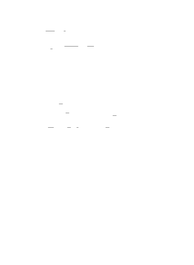
where

h1"ln(J1#y#Jy). Finally, after normalizing y to its average value SyT"2/c, we

obtain [71]:

P(I

I )Kexp

[ln

2(J1#2II/c#J2II/c)]

(7.24)

For I

I ;c, Eq. (7.24) reproduces the perturbative expansion (7.17), while for II<c it implies the

log-normal asymptotic behavior of the distribution P(I

I ):

ln P(I

I )K!(c/8)ln2(8II/c) .

(7.25)

The log-normal

`taila (7.25) should be contrasted with the stretched-exponential asymptotic

behavior of the distribution of transmission coe$cients, Eq. (7.9). As was found in [71], these two
results match each other in the following way. When the points z and z0 approach the sample

edges, z0"¸!z;¸, an intermediate regime of a stretched-exponential behavior emerges:

ln P(I

I )K

I #

I 2#2,

I ;g ,

JgII,

g;I

I ;g

g¸

8z0

2 II

I <g

(7.26)

Thus, when the source and the detector move toward the sample edges, the range of validity of the
stretched-exponential behavior becomes broader, while the log-normal

`taila gets pushed further

away. In contrast, when the source and the detector are located deep in the bulk, z0&¸!z&¸,

the stretched-exponential regime disappears, and the Rayleigh distribution crosses over directly to
the log-normal one at I

I &g.

Let us now describe the physical mechanisms standing behind these di!erent forms of P(I

I ) [71].

The Green's function G

R(r0,r) can be expanded in eigenfunctions of a non-Hermitean (due to open

boundaries)

`Hamiltoniana as

R(r0,r)"+

tHi(r0)ti(r)(k20!Ei#ici)~1 .

Since the level widths

ci are typically of order of the Thouless energy Ec&D/¸2, there is typically

g levels contributing appreciably to the sum. In view of the random phases of the wave

functions, this leads to a Gaussian distribution of G

R(r0,r) with zero mean, and thus to the Rayleigh

distribution of I(r0, r)"DGR(r0,r)D2, with the moments SIInT"n!. The stretched-exponential behav-

ior results from such disorder realizations where one of the states

ti has large amplitudes in both

the points r0 and r. Considering both ti(r0) and ti(r) as independent random variables with

Gaussian distribution and taking into account that only one (out of g) term contributes in this case
to the sum for G

R, we

"nd

SIInT&n!n!/gn, corresponding to the above stretched-exponential form

of P(I

I ). Finally, the log-normal asymptotic behavior corresponds to those disorder realizations

where G

R is dominated by an anomalously localized state, which has an atypically small width ci

359

A.D. Mirlin / Physics Reports 326 (2000) 259}382

(the same mechanism determines the log-normal asymptotics of the distribution of local density of
states, see Section 4.3).

8. Statistics of energy levels and eigenfunctions in a ballistic system with surface scattering

In the preceding part of this article we considered statistical properties of spectra of disordered

di!usive systems. Using the supersymmetric

p-model approach, we were able to demonstrate the

relevance of the random matrix theory (RMT) and to calculate deviations from its predictions both
for the level and eigenfunction statistics. Generalization of these results to the case of a chaotic
ballistic system (i.e. quantum billiard) has become a topic of great research interest. For ballistic
disordered systems the

p-model has been proposed [75], with the Liouville operator replacing the

di!usion operator in the action. It has also been conjectured that the same

p-model in the limit of

vanishing disorder describes statistical properties of spectra of individual classically chaotic system.
This conjecture was further developed in [76,77,259] where the

p-model was obtained by means of

energy averaging, and the Liouville operator was replaced by its regularization } the Perron}
Frobenius operator.

However, straightforward application of the results of Refs. [10,11,25,27] to the case of an

individual chaotic system is complicated by the fact that the eigenvalues of the Perron}Frobenius
operator are unknown, while its eigenfunctions are extremely singular. For this reason the

p-model

approach has so far failed to provide explicit results for any particular ballistic system.

In this section, we consider a ballistic system with surface disorder leading to di!usive scattering

of a particle in each collision with the boundary. This models behavior of a quantum particle in
a box with a rough boundary which is irregular on the scale of the wave length. Since the particle
loses memory of its direction of motion after a single collision, this model describes a limit of an
`extremely chaotica ballistic system, with typical relaxation time being of order of the #ight time.
(This should be contrasted with the case of a relatively slight distortion of an integrable billiard
[196,260,261].) One might naively think that all results for such a model could be obtained by
setting l+¸ in a system with bulk disorder. In fact, the level statistics in a system with bulk
disorder and arbitrary relation between mean free path l and system size ¸ was studied in
[168,169,262]. However, the results presented below show that systems with bulk and surface
disorder are not equivalent.

To simplify the calculations, we will assume a circular geometry of the billiard. A similar problem

was studied numerically in Ref. [263,264] for a square geometry. We consider only the case of
unitary symmetry (broken time-reversal invariance); generalization to the orthogonal case is
straightforward. We follow Ref. [78] in the presentation below. The level statistics for the same
problem was independently studied in Ref. [79]. Very recently, the same approach was used [265]
to calculate the persistent current in a ring with di!usive scattering.

Our starting point is the sigma-model for ballistic disordered systems [31,75]. The e!ective

action for this model has the form

F[g(r, n)]"

dr Str

uKSg(r)T!

q(r)

Sg(r)T2!2vFSK;~1n+;T

(8.1)

A.D. Mirlin / Physics Reports 326 (2000) 259}382

360

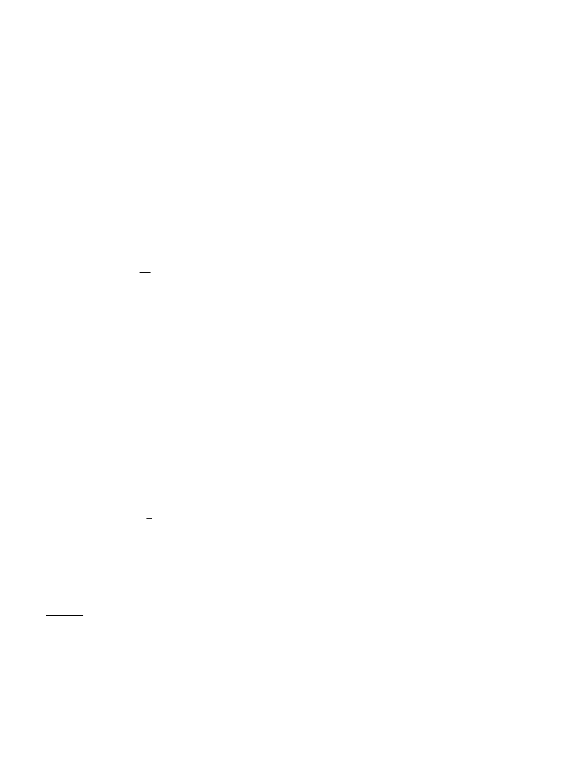
13 Exact form of the boundary condition depends on the underlying microscopic model. In particular, the di

!use

scattering can be modelled by surrounding the cavity by a disordered layer with a bulk mean free path l and a thickness
d<l. The corresponding boundary condition [268,269] di!ers from Eq. (8.3) by a parameterless function of order unity.
For a review of the boundary conditions corresponding to various microscopic realizations of the rough surface see
[270].

Here a 8

]8 supermatrix

"eld g is de"ned on the energy shell of the phase space, i.e. g depends on

the coordinate r and direction of the momentum n. The momentum dependence of the "eld
g distinguishes the ballistic

p-model from the di

!usive case where the supermatrix "eld Q depends

on r only. The angular brackets denote averaging over n:

SO(n)T":dn O(n) with the normalization

:dn"1. Like in the case of the di

!usive

p-model, the matrix g is constrained by the condition

2(r, n)"1, and can be represented as g";K;~1, with K"diag(1, 1, 1, 1,!1,!1,!1,!1).

Since we are interested in the clean limit with no disorder in the bulk, the second term in the action
(8.1) containing the elastic mean free time

q is zero everywhere except at the boundary where it

modi"es the boundary condition (see below).

As was explained in Section 2, the statistical properties of energy levels are governed by the

structure of the action in the vicinity of the homogeneous con"guration of the g-"eld, g(r, n)"

Writing ;"1!=/2#2, we "nd the action in the leading order in =,

F0[=]"!

dr dn Str [=21(KK!iu)=12] ,

(8.2)

where the indices 1, 2 refer to the

`advanced}retardeda decomposition of =, and KK is the Liouville

operator, K

K ,vFn+. This `linearizeda action has the same form as that of a di!usive system, with

the di!usion operator being replaced by the Liouville operator. This enables us to use the results
derived for the di!usive case by substituting the eigenvalues and eigenfunctions of the operator
K

K for those of the di!usion operator.

The operator K

K should be supplemented by a boundary condition, which depends on the form of

the surface roughness. As a model approximation we consider purely di!use scattering [266,267]
for which the distribution function

u(r, n) of the outgoing particles is constant and is

"xed by #ux

conservation:

u(r, n)"p

(

);0

(Nn

@)u(r, n@)dn@, (Nn)(0 .

(8.3)

Here the point r lies at the surface, and N is an outward normal to the surface. This boundary
condition should be satis"ed by the eigenfunctions of K

K .

The eigenvalues

j of the operator KK corresponding to angular momentum l obey the equation

I l(m),!1#

1
2

h sin h exp[2ilh#2m sin h]"0 ,

(8.4)

where

m,Rj/vF, and R is the radius of the circle. For each value of l"0,$1,$2,2 Eq. (8.4) has

a set of solutions

mlk with mlk"m~l,k"mHl,~k, which can be labeled with k"0,$1,$2,2 (even l)

or k"$1/2,$3/2,2 (odd l). For l"k"0 we have

m00"0, corresponding to the zero mode

361

A.D. Mirlin / Physics Reports 326 (2000) 259}382

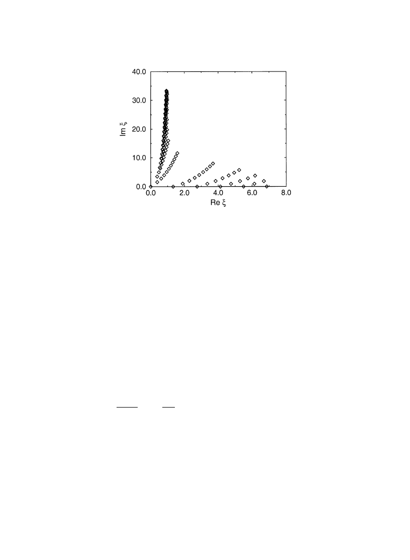
Fig. 13. First 11

]11 (04k, l(11) eigenvalues of the Liouville operator KK in units of vF/R, as given by Eq. (8.4). From

Ref. [78].

u(r, n)"const. All other eigenvalues have positive real part Re mlk'0 and govern the relaxation of

the corresponding classical system to the homogeneous distribution in the phase space.

The asymptotic form of the solutions of Eq. (8.4) for large

DkD and/or DlD can be obtained by using

the saddle-point method,

mkl+

0.66l#0.14 ln l#0.55

pik, 04k;l ,

(ln k)/4#

pi(k#1/8),

04l;k .

(8.5)

Note that for k"0 all eigenvalues are real, while for high values of k they lie close to the imaginary
axis and do not depend on l (see Fig. 13).

8.1. Level statistics, low frequencies

As was explained in Section 2.2 [see Eq. (2.27)], in the range of relatively low frequencies (which

for our problem means

u;vF/R, see below) the level correlation function R(s"u/D) has the form

R(s)!1"

d(s)!

sin

2ps

(

ps)2

pvF

sin

2ps .

(8.6)

The "rst two terms correspond to the zero-mode approximation and are given by RMT, while the
last one is the non-universal correction to the RMT results. The information about the operator
K

K enters through the dimensionless constant A"+@m~2

, where the prime indicates that the

eigenvalue

m00"0 is excluded. The value of A, as well as the high-frequency behavior of R(s) (see

below), can be extracted from the spectral function [9]

u)"+

Sl(u); Sl(u),+

(

jkl!iu)~2 .

(8.7)

A.D. Mirlin / Physics Reports 326 (2000) 259}382

362

According to the Cauchy theorem, Sl can be represented as an integral in the complex plane,

Sl(u)"

2 1

(z!i

uR/vF)2

I @l(z)

I l(z)

dz ,

where the contour C encloses all zeroes of the function J

I l(z). Evaluating the residue at z"iuR/vF,

we "nd

Sl(u)"!(R/vF)2

z/*uR@v

ln J

I l(z) .

(8.8)

Considering the limit

uP0 and subtracting the contribution of j00"0, we get

A"!19/27!175

p2/1152#64/(9p2)+!1.48 .

(8.9)

In contrast to the di!usive case, this constant is negative: the level repulsion is enhanced with
respect to result for RMT. Eq. (8.6) is valid as long as the correction is small compared to the RMT
result, i.e. provided

u is below the inverse time of

#ight, v

/R.

8.2. Level statistics, high frequencies

In the range

u<D the connected part of the level correlation function R(u)!1 can be

decomposed into the smooth Altshuler}Shklovskii (AS) part RAS(u)"(D2/2p2)ReS(u) [9] and

the part R04# which oscillates on the scale of the level spacing (see Section 2.2). Evaluating the

asymptotic behavior of Sl(u) from Eq. (8.8), we "nd in the high-frequency regime when u<vF/R:

RAS(u)"

puR

1@2

cos

(8.10)

The oscillating part of the level correlation function R04#(s) for frequencies u<D is given by

Eq. (2.34) with the spectral determinant

D(s)"s

~2 <

klE(00)

(1!is

D/jkl)~1(1#isD/jkl)~1 .

Since

D~2R2 ln D(s)/Rs2"!2Re S(u), we can restore D(s) from Eqs. (8.7), (8.8) up to a factor of the

form exp(c1#c2s), with c1 and c2 being arbitrary constants. These constants are "xed by the

requirement that Eq. (2.34) in the range

D;u;vF/R should reproduce the low-frequency

behavior (8.6). As a result, we obtain

D(s)"

6 1

I l(isN~1@2)JIl(!isN~1@2)

(8.11)

Here N"(vF/RD)2"(pFR/2)2 is the number of electrons below the Fermi level. For high

frequencies

u<vF/R this yields the following expression for the oscillating part of the level

correlation function:

R04#(u)"

128

cos

(8.12)

363

A.D. Mirlin / Physics Reports 326 (2000) 259}382

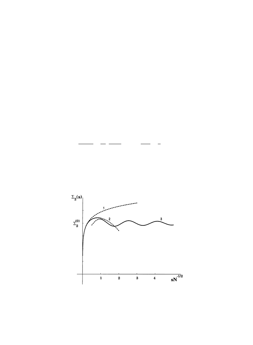
Fig. 14. Level number variance

R2(E) as a function of energy;s"E/D. Curve 1 shows the RMT result, while curves 2 and

3 correspond to asymptotic regimes of low (8.14) and high (8.15) frequencies. The saturation value

R(0)

is given in the text.

From Ref. [78].

It is remarkable that the amplitude of the oscillating part does not depend on frequency. This is in
contrast to the di!usive case, where in the AS regime (

u above the Thouless energy) the oscillating

part R04#(u) is exponentially small, see Eq. (2.39).

8.3. The level number variance

The smooth part of the level correlation function can be best illustrated by plotting the variance

of the number of levels in an energy interval of width E"s

R2(s)"

(s!

Ds8D)R(s8)ds8 .

(8.13)

A direct calculation gives for s;N

1@2

p2R2(s)"1#c#ln(2ps)#As2/(2N)

(8.14)

and for s<N

1@2

p2R2(s)"1#c#ln

16N

1@2

p2
16

1@2

cos

1@2

p
4

(8.15)

Here

c+0.577 is Euler

's constant, and

A is de"ned by Eq. (8.9). The "rst three terms at the rhs of

Eq. (8.14) represent the RMT contribution (curve 1 in Fig. 14).

As seen from Fig. 14, the two asymptotics (8.14) and (8.15) perfectly match in the intermediate

regime, s&N

1@2. Taken together, they provide a complete description of R2(s). According to

Eq. (8.15), the level number variance saturates at the value

R(0)

p~2(1#c#ln(16N1@2/p2)), in

A.D. Mirlin / Physics Reports 326 (2000) 259}382

364

contrast to the behavior found for di!usive systems [9] or ballistic systems with weak bulk disorder
[168,262]. The saturation occurs at energies s&N

1@2, or in conventional units E&vF/R. This

saturation of

R2(s), as well as its oscillations on the scale set by short periodic orbits, is expected for

a generic chaotic billiard [80,81]. It is also in good agreement with the results for

R2(s) found

numerically for a tight-binding model with moderately strong disorder on boundary sites
[263,264].

8.4. Eigenfunction statistics

Now we turn to correlations of the amplitudes of an eigenfunction in two di!erent points de"ned

by Eq. (3.67). As was discussed in Section 3.3.3, these correlations are governed by the ballistic
propagator

PB(r1,r2) (see Eq. (3.98) and the text preceding it). Direct calculation gives:

PB(r1,r2)"P1(r1,r2)#P2(r1,r2) ,

(8.16)

P1(r1,r2)"P(0)B(r1!r2)!<~1

@1 P(0)B(r@1!r2)

@2 P(0)B(r1!r@2)#<~2

@1 dr@2 P(0)B(r@1!r@2) ,

(8.17)

P2(r1,r2)"

ppFR

k/1

2!1

r1r2

cos k(

h1!h2)

where

P(0)

(r)"1/(

ppFDrD), and (r,h) are the polar coordinates. This formula has a clear interpreta-

tion. The function

PB can be represented as a sum over all paths leading from r1 to r2, with

possible surface scattering in between. In particular,

P1 corresponds to direct trajectories from

r1 to r2 with no re#ection from the surface, while the contribution P2 is due to the surface

scattering. The "rst term in the numerator 4k

2!1 comes from trajectories with only one surface

re#ection, while the second sums up contributions from multiple re#ections.

Let us summarize the main results of this section. We have used the ballistic

p-model approach

to study statistical properties of levels and eigenfunctions in a billiard with di!usive surface
scattering, which exempli"es a ballistic system in the regime of strong chaos. It was found that the
level repulsion and the spectral rigidity are enhanced compared to RMT. In particular, the level
number variance saturates at the scale of the inverse time of #ight, in agreement with Berry's
prediction for a generic chaotic system [80,81]. As another manifestation of the strong spectral
rigidity, the oscillating part of the level correlation function does not vanish at large level
separation. We calculated also the ballistic analog of the di!usion propagator in this model, which
governs correlations of eigenfunction amplitudes in di!erent spatial points.

While we focused our attention on the statistics of levels and wave functions in a closed ballistic

sample, the surface nature of scattering will also modify statistical properties of the transport
characteristics for an open system. In this connection, we mention the recent papers [271,272]
where quantum localization and #uctuations of the transmission coe$cients and of the conduc-
tance were studied for a quasi-1D wire with a rough surface. A number of important di!erences
compared to the case of bulk disorder was found.

365

A.D. Mirlin / Physics Reports 326 (2000) 259}382

Note that the motion in a quasi-1D wire with surface scattering is closely related to the PRBM

ensemble of Section 5.3. According to (8.3), the probability density for a particle to leave the surface
after a scattering event with an angle

h;1 with respect to the surface is P(h)&h. Since the

distance of the ballistic #ight is r&

h~1 for small h, this yields P(r)&r~3 for r larger than the

transverse size of the wire. Thus, we get a power-law

`taila at large r of the form (5.43) with a"3/2.

According to Section 5.2, this is precisely the marginal value separating the regions of conventional
K

(q, 0)Jq

2 and unconventional K~1

(q, 0)Jq

2a~1 behavior of the di

!usion

propagator

K0(q, u). It is clear that at a"3/2 the propagator acquires a logarithmic correction,

(q, 0)Jq

2 ln q, see Ref. [271] for details.

9. Electron}electron interaction in disordered mesoscopic systems

In the preceding sections we have considered statistical properties of energy levels and eigenfunc-

tions of a single particle in a disorder potential. However, if an electronic system is considered, the
Coulomb interaction between the electrons has to be taken into account. The in#uence of the
electron}electron interaction on transport properties of disordered systems has been intensively
studied during the last two decades, in particular in connection with such phenomena as weak
localization [273] and universal conductance #uctuations [274]. The electron}electron interaction
sets the length scale l

(

(phase breaking length) below which the electron wave function preserves its

coherence. Also, interplay of the interaction and disorder leads to a singular (at Fermi energy or at
zero temperature) correction to the density of states and to the conductivity [273].

More recently, another kind of problems has attracted the research interest: to what extent does

the electron}electron interaction in#uence the properties of the electron spectrum in a disordered
dot? This interest is largely motivated by a recent progress in nanotechnology which allows to
observe experimentally discrete electronic levels in semiconductor quantum dots [93,275] and in
small metallic grains [276,277]. In fact, there are two types of the quantum dot spectra studied
experimentally via measuring their I}< characteristics: (i) excitation spectrum, when excited levels
are probed in a dot with given number of electrons by increasing the source-drain voltage, and
(ii) addition spectrum, when electrons are added one by one by changing the gate voltage.

As concerns the excitation spectrum, it was found in [99,278] that the quasiparticle levels with

energies below the Thouless energy Ec (counted from the Fermi energy) have a width smaller than

the mean level spacing and thus form a well-de"ned discrete spectrum. To show this, let us calculate
the r.m.s. value of the matrix element <ijkl of the screened Coulomb interaction which describes

a decay of the quasiparticle state

DiT to a three-particle (more precisely, two particles#one hole)

state

D jklT. Using Eqs. (3.78), (3.88) for a di

!usive dot, one "nds [99]

SD<ijklD2T&(D/g)2. On the

other hand, the density of states of the three-particle states is

l3(E)&E2/D3, so that the Golden

Rule width of the one-particle states is

C(E)"2pSD<D2Tl3(E)&E2/Dg2. Comparing C(E) with D,

we get the above threshold E&g

D"Ec. The number of the discrete excited levels is thus of order

of the intrinsic dimensionless conductance g of the dot (not to be confused with the tunneling
conductance in the Coulomb blockade regime determined by the contacts). These "ndings are in
agreement with experiment [93].

The "ne structure of these excited single particle levels was studied theoretically in [100,279,280]

(see also Refs. [325,326]) where the Hamiltonian of the many-body interacting problem was

A.D. Mirlin / Physics Reports 326 (2000) 259}382

366

considered as a tight-binding model in the Fock space, with matrix elements of the Coulomb
interaction playing a role of the hopping terms. It was found that only for the energy above
E

JgD is the Golden Rule applicable and the levels have the regular Lorentzian shape. For

smaller energies the quasiparticle excitation consist essentially of a single peak with a small
admixture of other many-particle exact eigenstates. This corresponds to the Anderson localization
in the Fock space.

Though the properties of the single-particle excitations discussed above are of most interest,

one can also discuss statistical properties of exact many-body levels. For excitation energy
E<

D a typical state consists of &JE/D<1 quasiparticles, each of them having an energy

JED. Comparing the density of those states to which any of such states is coupled with the

matrix element of the interaction, one estimates the border for the complete delocalization of
many-body states as Ech&*g2@3 [279,281] (see also [282]). For energies E;Ech the many-body

level statistics is Poissonnian, while for the energies above Ech it should acquire the Wigner}Dyson

form. Numerical studies of statistical properties of spectra of many-body fermionic systems
[283}287] indeed show such a crossover from the Poisson to RMT statistics with increasing
excitation energy.

Statistical properties of the addition spectrum have been studied by several experimental groups

recently [83,86,288}290]. We will address the theoretical aspects of this problem (following Refs.
[84,136]) in Section 9.1.

Let us brie#y mention another topic which has attracted a great deal of research interest recently.

This is the problem of localization of two interacting particles raised by Shepelyansky [291] (see
also an early paper by Dorokhov [292]). It was suggested in [291] that the e!ective localization
length

m2 of two interacting particles in a 1D disordered sample can be much larger than the

localization length

m1 of a non-interacting particle. This paper stimulated a considerable analytical

and numerical activity. In the quasi-1D case, the problem can be mapped onto an ensemble of
random banded matrices with strongly #uctuating diagonal elements, which was studied numer-
ically in [293] and analytically (via the supersymmetric

p-model approach) in [294,295]. The

results con"rmed the original conjecture of Shepelyansky,

m2Jm21. In the case of a strictly 1D

system, the situation is somewhat more complicated, since the corresponding random matrix
ensemble was found [61] to be of the power-law random banded matrix type (see Section 5.3) in the
critical regime

a"1. Still, the localization length enhancement was predicted, m2Jmk1, but with

a non-universal exponent

k (1(k(2) depending on the interaction strength. Generalization of

the Shepelyansky's idea to the vicinity of the Anderson transition point in higher-dimensional
systems was proposed by Imry [296]. A detailed review of recent activity in this direction can be
found in [89].

9.1. Coulomb blockade: yuctuations in the addition spectra of quantum dots

The Coulomb blockade e!ect shows up the most distinctly in the addition spectrum experiment,

where one measures the conductance of an almost isolated quantum dot as a function of the gate
voltage. Detailed description of the experimental setup can be found, e.g. in [82,297]. At low
temperature ¹ one observes a sequence of almost equidistant peaks separated by

`valleysa where

the conductance is very small. The positions of the peaks are determined by the condition that the
energies of the dot with N and N#1 electrons are equal. We will assume below that the following

367

A.D. Mirlin / Physics Reports 326 (2000) 259}382

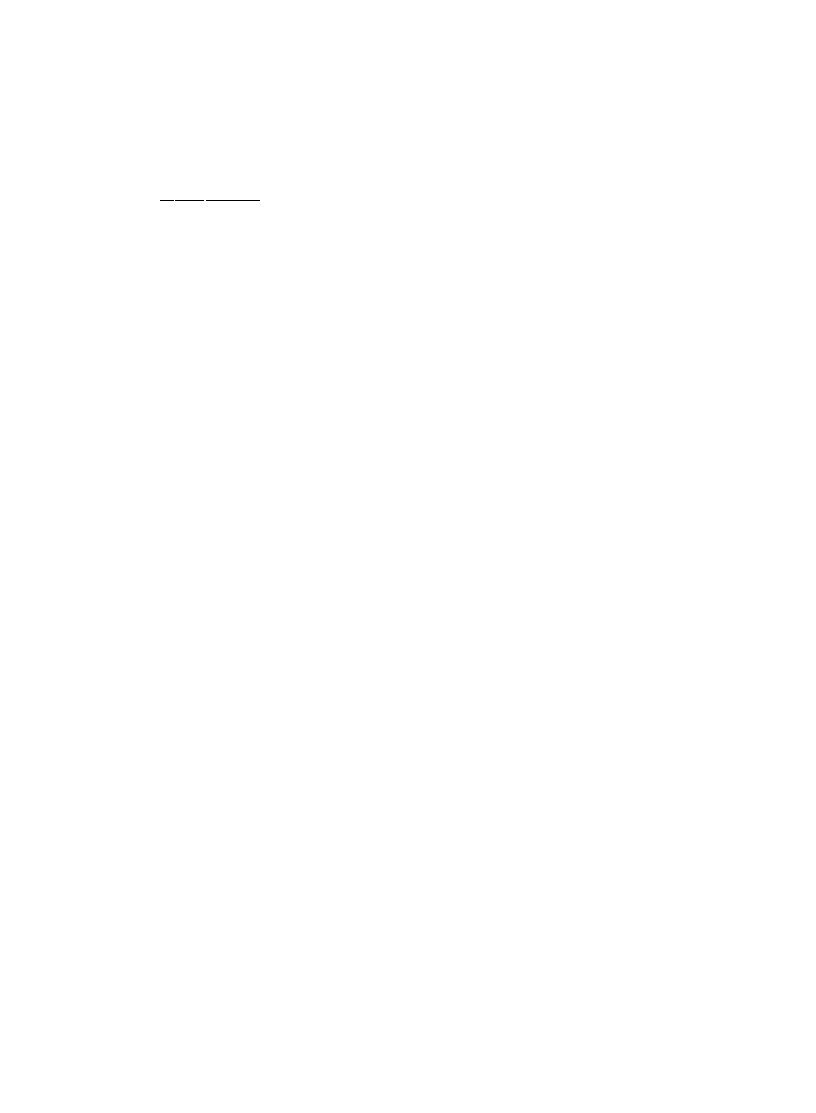
inequality is met:

C;k¹;D, where C"Cl#Cr is the sum of the tunneling rates to the leads.

The peak width is then set by the temperature, while the height is given by [298]

g.!9"

2k¹

ClCr

Cl#Cr

(9.1)

The peak heights show strong #uctuations induced by RMT-like #uctuations of eigenfunction
amplitudes, as predicted in [13,96] and observed experimentally in [94,95]. In the valleys between
the peaks, it is energetically costly (of order of the charging energy e

2/C, where C is the dot

capacitance) to add an electron to (or to remove from) the dot, and the conductance is determined
by virtual processes (so-called elastic cotunneling [299]) and is strongly suppressed.

The issue of the statistics of the peak spacings was addressed for the "rst time in [83]. Basing on

numerical data for very small systems, the authors of [83] concluded that the r.m.s. deviation of the
peak spacing SN is proportional to the charging energy e2/C, with a coe$cient +0.15. We will

show below (our consideration will closely follow Refs. [84,136]) that the #uctuations are in fact
much smaller, of order of the mean level spacing

D. Let us note that in an analogous problem for

classical particles the #uctuation magnitude rms(SN) would indeed be proportional to the mean

value

SSNT [300,301]. The physical reason for smaller #uctuations in the quantum case is in the

delocalized nature of the electronic wave functions, which are spread roughly uniformly over the
system. These theoretical conclusions were con"rmed recently by thorough experimental studies,
as discussed in the end of the section.

The simplest theoretical model which may be used to study distribution of the peak spacings is as

follows. One considers a dot as a "xed size di!usive mesoscopic sample and assumes that changing
a gate voltage by an amount

d<g simply reduces to a uniform change of the potential inside the dot

by a constant

c d<g, with certain numerical coe$cient c (`lever arma). Such a model was used for

numerical simulations of the addition spectra in Refs. [83,302]. We start by considering the
statistics of peak spacings within this model [84]; we will later return to the approximations
involved and relax some of them. We will neglect the spin degree of freedom of electrons "rst;
inclusion of the spin will be also discussed in the end of the section.

The distance between the two consecutive conductance peaks is given by (Fig. 15)

SN"(EN`2!EN`1)!(EN`1!EN)

kN`2

N`1

kN`1

(9.2)

where EN is the ground state of a sample with N electrons. In the second line of Eq. (9.2) we rewrote

SN in terms of the Hartree}Fock single electron energy levels, with kji denoting the energy of the

state

dj in the dot containing i electrons. It is convenient to decompose SN in the following way

SN"(kN`2

N`1

kN`2

)#(

kN`2

kN`1

)

E1#E2 .

(9.3)

The quantity E2 is the distance between the two levels of the same one-particle (Hartree}Fock)

Hamiltonian H

K N (describing a dot with N electrons) and is expected to obey RMT; in particular

SE2T"D and r.m.s.(E2)"aD with a numerical coe$cient a of order of unity [a"0.52 (0.42) for

the orthogonal (resp. unitary) ensemble]. On the other hand, E1 is a shift of the level d(N#2) due

to the change of the Hamiltonian H

K NPHKN`1 accompanying addition of the electron d(N#1) to

the system.

A.D. Mirlin / Physics Reports 326 (2000) 259}382

368

Fig. 15. Energy levels before and after the electron

d(N#1) has been added to the dot. From Ref. [84].

The e!ective interaction ;(r, r

@) between the electrons d(N#1) and d(N#2) can be found

from the RPA-type equation,

;

(r, r

@)";0(r!r@)!

;0(r!r

)P0(r

, r

);(r

, r

(9.4)

where ;0(r)"e2/er, e is the dielectric constant, and

P0(r

, r

l[d(r

)!<

~1]

(9.5)

is the polarization operator. Its solution has the form [84]

;

(r, r

@)";M#d;(r)#d;(r@)#;i(r,r@) .

(9.6)

Here ;

M ,e2/C is a constant (charging energy), d;(r) is the change of the self-consistent potential

due to addition of one electron (i.e. di!erence in the self-consistent potential in the dots with N and
N#1 electrons), and ;i(r) is the screened Coulomb interaction. In particular, in the experi-

mentally most relevant 2D case (which we will consider below) and assuming a circular form of the
dot with radius R, we have

d;(r)"!

eisR

2!r2)~1@2 ,

(9.7)

while ;i is given in the Fourier space by ;Ii(q)"2pe2/e(q#is) with the inverse screening length

is"2pe2l/e.

According to Eq. (9.6), the term E1 can be decomposed into the following three contributions:

E1"e2/C#

dr(

Dt2N`1(r)D#Dt2N`2(r)D)d;(r)#

dr dr

@Dt2N`1(r)DDt2N`2(r@)D;i(Dr!r@D)

(0)

(1)

(2)

(9.8)

369

A.D. Mirlin / Physics Reports 326 (2000) 259}382

The "rst term in Eq. (9.8) (the charging energy) determines the average value

SE1T and thus the

average peak spacing

SSNT (since e2/C<D for a large dot with N<1). This is the only contribu-

tion to E1 kept by the so-called constant interaction model, which in addition neglects #uctuations

of the capacitance C. Consequently, #uctuations of SN within the constant interaction model are

determined solely by #uctuations of the single-particle level spacing E2 and thus follow RMT:

r.m.s.(SN)"aD.

The term E1 in Eq. (9.3) is however an additional source of #uctuations and is thus responsible

for the enhancement of #uctuations in comparison with RMT. In principle, all the three terms E

(0)

(1)

, and E

(2)

in Eq. (9.8) contribute to this enhancement. Fluctuations of the "rst one, E

(0)

2/C

are due to the fact that the capacitance is slightly di!erent from its purely geometric value because
of a "nite value of the screening length. The corresponding correction to C can be expressed in
terms of the polarization operator P(r, r

@). The latter is a

#uctuating quantity (because of #uctu-

ations of the eigenfunctions in the Fermi sea) and contains a random part P3(r, r@) leading to the

following expression for the random part of the charging energy:

2/C)3"2

dr dr

@ d;(r)P3(r,r@)d;(r@) .

(9.9)

Evaluating the #uctuations of the polarization operator, we "nd [138]

var(E

(0)

l2 ln g

d;(r

)

P(r

, r

)

d;(r

)

1
b

ln g

(9.10)

Now we consider #uctuations of the last term, E

(2)

, in Eq. (9.8). Using Eqs. (3.74) and (3.86) for the

correlations of eigenfunction amplitudes in two remote points, the variance of E

(2)

is found to be

var(E

(2)

b2<4

;i(Dr

D);i(Dr

D)P(r

, r

)

P(r@

, r

)

b2<2

P2(r

, r

(9.11)

Finally, #uctuations of the term E

(1)

can be also evaluated with a help of Eqs. (3.74), (3.86), yielding

var(E

(1)

b<2

d;(r

)

P(r

, r

)

d;(r

(9.12)

It is seen that for g<1 all the contributions Eqs. (9.10)}(9.12) are parametrically small compared

to the RMT #uctuations (which are &

D). Fluctuations of the term E(1)

related to the change

d;(r)

of the self-consistent potential represent parametrically leading contribution to the enhancement of
the peak spacing #uctuations with respect to RMT.

Let us now discuss approximations made in the course of the above derivation:

(i) The dot was supposed to be di!usive in the calculation. For a ballistic dot one should replace

P(r, r@) by its ballistic counterpart. This would mean that the parameter g is replaced by
&

1@2&¸/jF, where N is the number of electrons in the dot and ¸ the characteristic linear

dimension. The numerical coe$cient would depend, however, on

`how strongly chaotica is the

dot. The role of the eigenfunctions #uctuations and correlations (

`scarsa) in enhancement of

A.D. Mirlin / Physics Reports 326 (2000) 259}382

370

the peak spacing #uctuations was studied in [303] via numerical simulations of a dot with
N+100 electrons.

(ii) It was assumed that changing the gate voltage results in a spatially uniform change of the

potential in the sample. This has led us to the expression Eq. (9.7) for the change of the
self-consistent potential

d;(r) accompanying the addition of one electron to the dot. This

result would correspond to a gate located far enough from the sample. In a more realistic
situation, when the gate is relatively narrow and located close to the sample, the potential
change

d;(r) (as well as the additional electron density) will be concentrated on the side of the

dot facing the gate. The change of the potential

d;(r) corresponds then to a slight deformation

of the dot with adding each electron to it. To estimate

d;(r) in this case, we can consider

a model problem of a point-like charged object (modeling the gate) located a distance d from
the edge of the dot. Assuming that the dot size is larger than d, we can approximate the dot
[while calculating

d;(r)] by a half plane. In one period of the Coulomb blockade oscillations

the gate charge changes by e (electron charge). The charge distribution induced in the dot is

do(x, y)"!

J(d#x)2#y2

(9.13)

where the closest to the gate point of the dot is chosen as the coordinate origin and the x axis is
directed along the dot edge. The corresponding change of the potential is

d;(r)"(e2l/e)~1do(r).

Substituting this into the "rst line of Eq. (9.12), we come to the same result

r.m.s.(E

(1)

D/Jbg ,

in the di!usive limit d'l, and to

r.m.s.(E

(1)

D/JbkFd

in the case d(l.
E!ect of the quantum dot deformation on the peak spacing #uctuations has been recently
considered in Ref. [304]. The authors of [304] characterized the strength of the deformation
by a phenomenological dimensionless parameter x and assumed that it can be large (x

Z1),

strongly a!ecting the spacing distribution. However, the above estimates indicate that for
a typical geometry this parameter is much less than unity, x&1/

Jg or x&1/JkFd.

(iii) It was assumed that the dot energy and the measured gate voltage are related through

a constant (or smoothly varying) coe$cient

c. This `lever arma c depends, however on the

dot-gate capacitance, which is also a #uctuating quantity. If the gate size and the distance to
the gate is of the order of the size of the dot, these #uctuations should be of the same order as

#uctuations of the dot self-capacitance and thus lead to additional #uctuations parametrically

small compared to

D, see Eq. (9.10).

(iv) The calculation was done within the random phase approximation, which assumes that the

ratio of the interparticle Coulomb energy to the kinetic energy is small, rs,J2e2/e+vF;1

(vF is the Fermi velocity). However, most of the experimental realizations of semiconductor

quantum dots correspond to rs+1. Since this value is still considerably lower than the Wigner

crystallization threshold, the calculations should be still valid, up to a numerical factor

a(rs)

[depending on rs only and such that a(rs;1)"1].

371

A.D. Mirlin / Physics Reports 326 (2000) 259}382

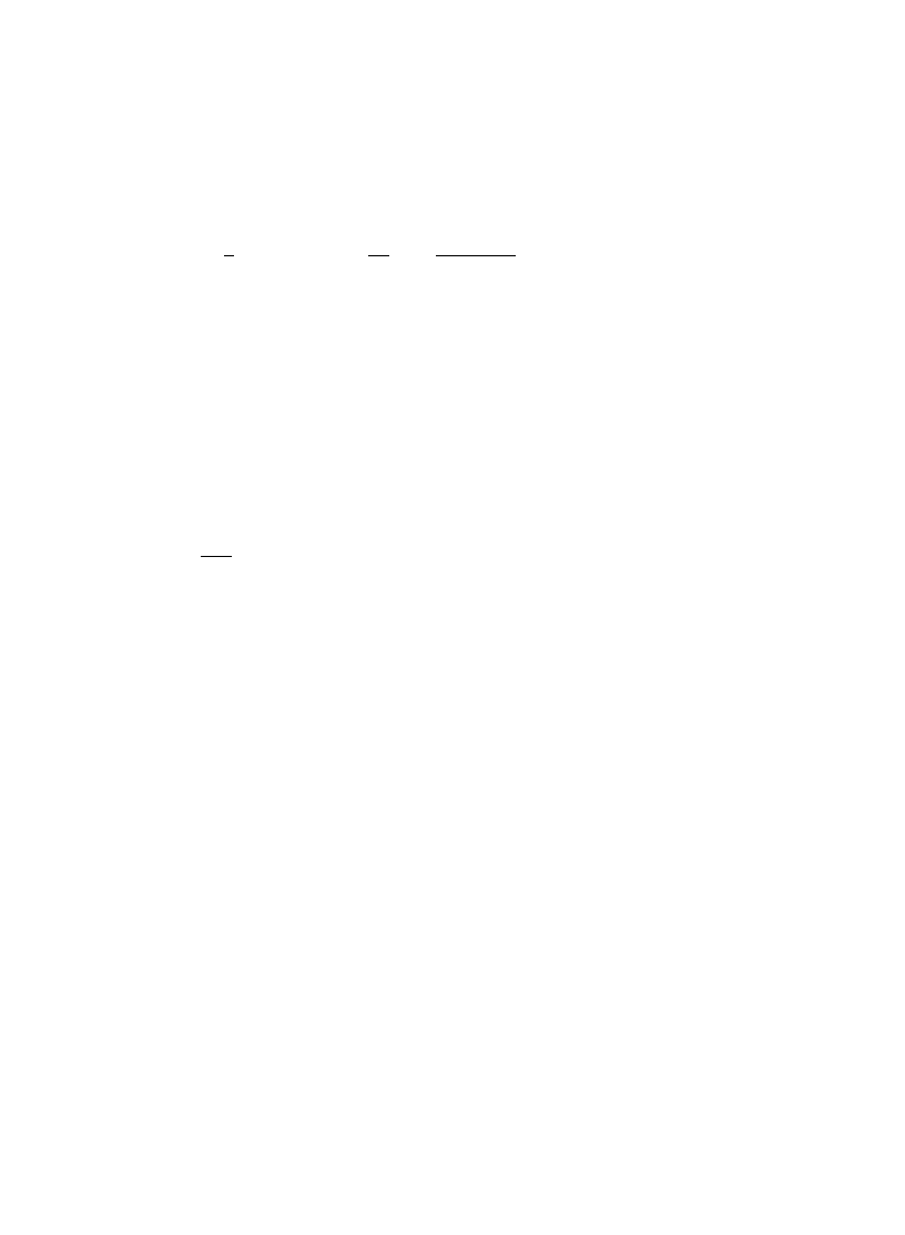
(v) We considered the model of spinless electrons up to now. Let us brie#y discuss the role of the

spin degree of freedom. Within the constant interaction model, it would lead to a bimodal
distribution [302] of peak spacings

P(SN)"

1
2

d(SN!e2/C)#

PWD

SN!e2/C

(9.14)

where PWD(s) is the Wigner}Dyson distribution and D denotes the level spacing in the absence

of spin degeneracy. The value of the coe$cient a in the relation r.m.s.(SN)"aD is then

increased (compared to the spinless case) and is equal to 1.24 (1.16) for the orthogonal (resp.
unitary) ensemble. Taking into account #uctuations of eigenfunctions (and thus of E1)

however modi"es the form of the distribution. The value of the term E

(2)

representing the

interaction between two electrons is larger in the case when

tN`2 and tN`1 correspondto two

spin-degenerate states (i.e. have the same spatial dependence of the wave function), since

dr dr

@Dt2i(r)DDt2i(r@)D;i(Dr!r@D)

dr dr

@Dt2i(r)DDt2j(r@)D;i(Dr!r@D)

b<2

dr dr

@ kd(Dr!r@D);i(Dr!r@D)&D

(9.15)

for rs&1 (the coe$cient depends on rs, see [84]). Therefore, "lling a state tit pushes up the

level

tis (with respect to other eigenstates) by an amount of order of D. This removes

a bimodal structure of the distribution of peak spacings and slightly modi"es the value of the
coe$cient a.

Basing on the above analysis, we can make the following general statement. Imagine that we "x

rs&1 (i.e. "x the electron density and thus the Fermi wave length) and the system geometry,

and then start to increase the linear dimension ¸ of the system. Then, while the average value
of the peak spacing SN scales as SSNT+e2/CJ1/¸, its #uctuations will scale di!erently:

r.m.s.(SN)&DJ1/¸2. This conclusion is also corroborated by diagrammatic calculations of

Ref. [85].

As was mentioned in the beginning of this section, this result should be contrasted with that for

classical particles [300,301], where the #uctuations are proportional to the mean value

SSNT. The

parametrically smaller #uctuations in the quantum case are due to the delocalized nature of the
electronic wave functions, which are spread roughly uniformly over the system.

The above prediction was con"rmed by recent experiments [86,87,290], where a thorough study

of the peak spacing statistics was carried out. It was found that the low-temperature value of
r.m.s.(SN), as well the typical temperature scale for its change are approximately given by the mean

level spacing

D (while in units of Ec the magnitude of #uctuations was as small as 1}4%).

Several recent papers studied statistical properties of the peak spacing numerically. Stopa [303]

used the density functional theory and found the #uctuations of the addition energies to be
approximately 0.7

D, in agreement with the above results. Disappearance of the bimodal character

of the peak spacing distribution with increasing rs was observed recently in numerical simulations

by Berkovits [305] via exact diagonalization. However, the system size and the number of particles

A.D. Mirlin / Physics Reports 326 (2000) 259}382

372

in the exact diagonalization studies are very small, so that it is di$cult to draw any quantitative
conclusions concerning the dots with large number of electrons from the results of [305].

10. Summary and outlook

In this article we have reviewed the recent progress in the study of statistical properties of

disordered electronic systems. We have discussed statistics of energy levels and eigenfunction
amplitudes, as well as of several related quantities (local density of states, escape time, conductance,
etc.) In most of the article the supersymmetric

p-model approach was used, as a unique and

powerful tool allowing one to calculate various distribution and correlation functions. Within this
approach, we have employed a number of complementary methods of treating the

p-model: exact

solution (in particular, transfer-matrix method in 1D), perturbation theory, renormalization group,
saddle-point method. The main emphasis has been put onto system-speci"c deviations from the
universal predictions of the random matrix theory. The results presented constitute a detailed and,
in many respects, complete description of #uctuations of spectra and wave functions of disordered
systems.

Still, there is a number of directions in this "eld in which a more complete understanding is

needed, so that the corresponding research remains active at present. Let us point out some of
them.

f Statistical properties of energy levels and wave functions of ballistic systems whose classical

counterparts are chaotic require more theoretical studies. It remains to be understood what are
the conditions of applicability of the ballistic

p-model derived in [75

}77]. Apparently, a certain

amount of disorder present in a system (or, in other words, some ensemble averaging) is needed
to justify the derivation in these papers, but the precise conditions have not been quanti"ed yet
(see Ref. [306] where this problem is discussed in the context of correlations of quantum maps).
Also, a discrepancy between the results of the

p-model and of the semiclassical approach in

treating repetitions of periodic orbits [307,308] is to be resolved. It remains to be seen whether
the ballistic

p-model approach can be developed to predict the weak-localization corrections

(recent attempts [309,310] did not lead to any de"nite conclusions), the asymptotic

`tailsa of the

distributions (like those discussed in Section 4 for di!usive systems), etc.

f Interplay of disorder and electron

}electron interaction in mesoscopic systems continues attract-

ing considerable research interest. In Section 9 of this article we discussed only the issue of

#uctuations in an (almost) closed system. In the experiment, coupling of the dot to the outside

world is controlled by the gate(s) and may be varied. There arise a rich variety of regimes
depending on the coupling strength, magnetic "eld, and the strength of the Coulomb interaction
(parameter rs). Fluctuations in open quantum dots have been studied recently, both theoretically

[311}313] and experimentally [289,290,314,315], but the issue is not fully understood yet. In Ref.
[316] it was found that application of a strong magnetic "eld a!ects dramatically the addition
spectrum of a quantum dot, leading to strong #uctuations and to bunching of the Coulomb
blockade peaks. A consistent explanation of these experimental results is still missing.

Very recently, several groups [317}321] simultaneously performed self-consistent Hartree}

Fock calculations of addition spectra of quantum dots. Though the method allows one to study

373

A.D. Mirlin / Physics Reports 326 (2000) 259}382

considerably larger systems as compared to the exact diagonalization method, the obtained
results were not su$cient to extract unambiguously a scaling dependence of the spacing
distribution function on the parameters of the problem. A drawback of the Hartree}Fock
method with the bare Coulomb potential is that the exchange interaction does not get screened,
whereas the screening was crucially important for the theoretical consideration in Section 9.1.
More work in this direction may be expected in the nearest future.

f The physics of the Anderson metal

}insulator transition, including #uctuations at the critical

point, remains an actively studied "eld. Parameters of modern computers allow one to evaluate
numerically critical indices and various distribution functions with a high accuracy. It would be
very interesting to study numerically the critical point in higher dimensions (see, in this respect,
recent paper [178]) as well as in an e!ectively in"nite-dimensional tree-like sparse random
matrix model and in a long-range 1D model (power-law random banded matrix ensemble
considered in Section 5.3). It remains to be seen what is the status of the conjecture of Ref. [49]
relating the spectral compressibility to the eigenfunction multifractality. Also, the form of the
conductance distribution at the critical point remains an open problem. Ref. [28] predicted
a log-normal form of the distribution function at g<

SgT&1, similarly to the distribution

functions of local density of states and of relaxation times. However, in contrast to the latter two
quantities, an anomalously large conductance cannot be explained by a single anomalously
localized state (since a single state cannot produce the conductance larger than 1). It seems much
more probable that the conductance distribution falls o! much more fast, in a Gaussian (or
similar) fashion at large g, but no corresponding calculation has been available so far. Tech-
nically, the problem is that calculating higher moments of the conductance requires increasing of
the size of the Q-matrix in the

p-model, which complicates tremendously a non-perturbative

treatment of the distribution function. For recent numerical studies of the conductance distribu-
tion at criticality, see Refs. [327}329].

Acknowledgements

My own work reviewed in this paper was done in collaboration with the late A.G. Aronov,

Ya.M. Blanter, F.-M. Dittes, Y.V. Fyodorov, V.E. Kravtsov, A. MuKller-Groeling, B.A. Muzykan-
tskii, R. Pnini, T. Seligman, B. Shapiro, M.R. Zirnbauer. It is my pleasure to thank all of them. I am
also indebted to many other colleagues, in particular, O. Agam, B.L. Altshuler, R. Berkovits,
S. Fishman, K. Frahm, Y. Gefen, D.E. Khmelnitskii, I.V. Lerner, L.S. Levitov, C. Marcus,
K. Muttalib, D.G. Polyakov, P.G. Silvestrov, I.E. Smolyarenko, A.M. Tsvelik, P. WoKl#e, and
I.Kh. Zharekeshev for numerous stimulating discussions of the topics addressed in the review. This
work was supported by SFB195 der Deutschen Forschungsgemeinschaft.

Appendix A. Abbreviations

AKL

Altshuler, Kravtsov, and Lerner, Ref. [28]

ALS

anomalously localized state

DMPK

Dorokhov-Mello-Pereira-Kumar (equations)

DOS

density of states

A.D. Mirlin / Physics Reports 326 (2000) 259}382

374

GOE

Gaussian orthogonal ensemble

GSE

Gaussian symplectic ensemble

GUE

Gaussian unitary ensemble

IPR

inverse participation ratio

LDOS

local density of states

logarithmically normal

PRBM

power-law random banded matrix

RBM

random banded matrix

renormalization group

RPA

random phase approximation

RMT

random matrix theory

Wigner}Dyson (level statistics)

1D, 2D, 3D one dimensional, two dimensional, three dimensional

References

[1] E.P. Wigner, Ann. Math. 53 (1951) 36.
[2] F.J. Dyson, J. Math. Phys. 3 (1962) 140.
[3] M.L. Mehta, Random Matrices, Academic Press, Boston, 1991.
[4] O. Bohigas, M.J. Giannoni, C. Schmit, Phys. Rev. Lett. 52 (1984) 1.
[5] L.P. Gor'kov, G.M. Eliashberg, Zh. Eksp. Theor. Fiz. 48 (1965) 1407 [Sov. Phys. JETP 21 (1965) 940].
[6] K.B. Efetov, Adv. Phys. 32 (1983) 53.
[7] K.B. Efetov, Supersymmetry in Disorder and Chaos, Cambridge University Press, Cambridge, 1997.
[8] J.J.M. Verbaarschot, H.A. WeidenmuKller, M.R. Zirnbauer, Phys. Rep. 129 (1985) 367.
[9] B.L. Altshuler, B.I. Shklovskii, Zh. Eksp. Theor. Fiz. 91 (1986) 220 [Sov. Phys. JETP 64 (1986) 127].

[10] V.E. Kravtsov, A.D. Mirlin, Pis'ma Zh. Eksp. Teor. Fiz. 60 (1994) 645 [JETP Lett. 60 (1994) 656].
[11] A.V. Andreev, B.L. Altshuler, Phys. Rev. Lett. 75 (1995) 902.
[12] C.E. Porter, Statistical Theories of Spectra: Fluctuations, Academic Press, New York, 1965.
[13] R.A. Jalabert, A.D. Stone, Y. Alhassid, Phys. Rev. Lett. 68 (1992) 3468.
[14] J. Stein, H.-J. StoKckmann, Phys. Rev. Lett. 68 (1992) 2867.
[15] A. Kudrolli, V. Kidambi, S. Sridhar, Phys. Rev. Lett. 75 (1995) 822.
[16] H. Alt, H.-D. GraKf, H.L. Harney, R. Ho!erbert, H. Lengeler, A. Richter, P. Schardt, H.A. WeidenmuKller, Phys. Rev.

Lett. 74 (1995) 62.

[17] A.D. Mirlin, Y.V. Fyodorov, J. Phys. A: Math. Gen. 26 (1993) L551.
[18] Y.V. Fyodorov, A.D. Mirlin, Int. J. Mod. Phys. B 8 (1994) 3795.
[19] A.D. Mirlin, Y.V. Fyodorov, Phys. Rev. Lett. 72 (1994) 526.
[20] A.D. Mirlin, Y.V. Fyodorov, J. de Phys. I France 4 (1994) 655.
[21] Y.V. Fyodorov, A.D. Mirlin, Phys. Rev. Lett. 69 (1992) 1093, 1832 (E).
[22] Y.V. Fyodorov, A.D. Mirlin, Phys. Rev. Lett. 71 (1993) 412.
[23] Y.V. Fyodorov, A.D. Mirlin, Pis'ma Zh. Eksp. Teor. Fiz. 58 (1993) 636 [JETP Lett. 58 (1993) 615].
[24] Y.V. Fyodorov, A.D. Mirlin, Pis'ma Zh. Eksp. Teor. Fiz. 60 (1994) 779 [JETP Lett. 60 (1994) 790].
[25] Y.V. Fyodorov, A.D. Mirlin, Phys. Rev. B 51 (1995) 13 403.
[26] Ya.M. Blanter, A.D. Mirlin, Phys. Rev. B 53 (1996) 12 601.
[27] Ya.M. Blanter, A.D. Mirlin, Phys. Rev. E 55 (1997) 6514.
[28] B.L. Altshuler, V.E. Kravtsov, I.V. Lerner, in: B.L. Altshuler, P.A. Lee, R.A. Webb (Eds.), Mesoscopic Phenomena

in Solids, North-Holland, Amsterdam, 1991, p. 449.

[29] B.A. Muzykantskii, D.E. Khmelnitskii, Phys. Rev. B 51 (1995) 5480.

375

A.D. Mirlin / Physics Reports 326 (2000) 259}382

[30] A.D. Mirlin, Pis'ma Zh. Eksp. Teor. Fiz. 62 (1995) 583 [JETP Lett. 62 (1995) 603].
[31] B.A. Muzykantskii, D.E. Khmelnitskii, preprint cond-mat/9601045.
[32] V.I. Fal'ko, K.B. Efetov, Europhys. Lett. 32 (1995) 627.
[33] V.I. Fal'ko, K.B. Efetov, Phys. Rev. B 52 (1995) 17 413.
[34] A.D. Mirlin, Phys. Rev. B 53 (1996) 1186.
[35] A.D. Mirlin, Y.V. Fyodorov (1995), unpublished.
[36] A.D. Mirlin, J. Math. Phys. 38 (1997) 1888.
[37] V.E. Kravtsov, I.V. Yurkevich, Phys. Rev. Lett. 78 (1997) 3354.
[38] C. Basu, C.M. Canali, V.E. Kravtsov, I.V. Yurkevich, Phys. Rev. B 57 (1998) 14 174.
[39] P.A. Lee, T.V. Ramakrishnan, Rev. Mod. Phys. 57 (1985) 287.
[40] B.L. Altshuler, I.K. Zharekeshev, S.A. Kotochigova, B.I. Shklovskii, Zh. Eksp. Theor. Fiz. 94 (1988) 343 [Sov.

Phys. JETP 67 (1988) 625].

[41] B.I. Shklovskii, B. Shapiro, B.R. Sears, P. Lambrianides, H.B. Shore, Phys. Rev. B 47 (1993) 11 487.
[42] V.E. Kravtsov, I.V. Lerner, B.L. Altshuler, A.G. Aronov, Phys. Rev. Lett. 72 (1994) 888.
[43] A.G. Aronov, A.D. Mirlin, Phys. Rev. B 51 (1995) 6131.
[44] V.E. Kravtsov, I.V. Lerner, Phys. Rev. Lett. 74 (1995) 2563.
[45] B.R. Sears, H.B. Shore, Statistical #uctuations of energy levels spectra near the metal-insulator transition, 1994,

unpublished.

[46] I. Zharekeshev, B. Kramer, in: H.A. Cerdeira, B. Kramer, G. SchoKn (Eds.), Quantum Transport in submicron

structures, NATO ASI Series E, Vol. 291, Kluwer Academic Publishers, Dordrecht, 1995, p. 93.

[47] I. Zharekeshev, B. Kramer, Jpn. J. Appl. Phys. 34 (1995) 4361.
[48] D. Braun, G. Montambaux, M. Pascaud, Phys. Rev. Lett. 81 (1998) 1062.
[49] J.T. Chalker, V.E. Kravtsov, I.V. Lerner, Pis'ma Zh. Eksp. Teor. Fiz. 64 (1996) 355 [JETP Lett. 64 (1996) 386].
[50] F. Wegner, Z. Phys. B 36 (1980) 209.
[51] C. Castellani, L. Peliti, J. Phys. A: Math. Gen. 19 (1986) L429.
[52] M. Schreiber, H. Grussbach, Phys. Rev. Lett. 67 (1991) 607.
[53] W. Pook, M. Janssen, Z. Phys. B 82 (1991) 295.
[54] B. Huckestein, B. Kramer, L. Schweitzer, Surf. Sci. 263 (1992) 125; B. Huckestein, L. Schweitzer, in: G. Landwehr

(Ed.), High Magnetic Fields in Semiconductor Physics III. Proc. Int. Conf. WuKrzburg 1990, Springer Series in
Solid State Sciences, Vol. 101, Springer, Berlin, 1992, p. 84.

[55] M. Janssen, Int. J. Mod. Phys. B 8 (1994) 943.
[56] B. Huckestein, Rev. Mod. Phys. 67 (1995) 357.
[57] A.D. Mirlin, Y.V. Fyodorov, F.-M. Dittes, J. Quezada, T.H. Seligman, Phys. Rev. B 54 (1996) 3221.
[58] J.V. Jose, R. Cordery, Phys. Rev. Lett. 56 (1986) 290.
[59] B.L. Altshuler, L.S. Levitov, Phys. Rep. 288 (1997) 487.
[60] A.V. Balatsky, M.I. Salkola, Phys. Rev. Lett. 76 (1996) 2386.
[61] I.V. Ponomarev, P.G. Silvestrov, Phys. Rev. B 56 (1997) 3742.
[62] M.A. Skvortsov, V.E. Kravtsov, M.V. Feigel'man, Pis'ma Zh. Eksp. Teor. Fiz. 68 (1998) 78 [JETP Lett. 68 (1998) 84].
[63] S. Iida, H.A. WeidenmuKller, J.A. Zuk, Ann. Phys. (NY) 200 (1990) 219.
[64] M.R. Zirnbauer, Phys. Rev. Lett. 69 (1992) 1584.
[65] A.D. Mirlin, A. MuKller-Groeling, M.R. Zirnbauer, Ann. Phys. (NY) 236 (1994) 325.
[66] P.W. Brouwer, K. Frahm, Phys. Rev. B 53 (1996) 1490.
[67] A.D. Mirlin, A. MuKller-Groeling (1994), unpublished.
[68] V. Plerou, Z. Wang, Phys. Rev. B 58 (1998) 1967.
[69] A. Ishimaru, Wave Propagation and Scattering in Random Media, Academic Press, New York, 1978.
[70] B. Shapiro, Phys. Rev. Lett. 57 (1986) 2168.
[71] A.D. Mirlin, R. Pnini, B. Shapiro, Phys. Rev. E 57 (1998) R6285.
[72] Th.M. Nieuwenhuizen, M.C.W. van Rossum, Phys. Rev. Lett. 74 (1995) 2674.
[73] E. Kogan, M. Kaveh, Phys. Rev. B 52 (1995) R3813.
[74] S.A. van Langen, P.W. Brouwer, C.W.J. Beenakker, Phys. Rev. E 53 (1996) R1344.
[75] B.A. Muzykantskii, D.E. Khmelnitskii, Pis'ma Zh. EDksp. Teor. Fiz. 62 (1995) 68 [JETP Lett. 62 (1995) 76].

A.D. Mirlin / Physics Reports 326 (2000) 259}382

376

[76] A.V. Andreev, O. Agam, B.D. Simons, B.L. Altshuler, Phys. Rev. Lett. 76 (1996) 3947.
[77] A.V. Andreev, B.D. Simons, O. Agam, B.L. Altshuler, Nucl. Phys. B 482 (1996) 536.
[78] Ya.M. Blanter, A.D. Mirlin, B.A. Muzykantskii, Phys. Rev. Lett. 80 (1998) 4161.
[79] V. Tripathi, D.E. Khmelnitskii, Phys. Rev. B 58 (1998) 1122.
[80] M.V. Berry, Proc. Roy. Soc. London A 400 (1985) 229.
[81] M.V. Berry, in: M.-J. Giannoni, A. Voros, J. Zinn-Justin (Eds.), Chaos and Quantum Physics, North-Holland,

Amsterdam, 1991, p. 251.

[82] L.P. Kouwenhoven, C.M. Marcus, P.L. McEuen, S. Tarucha, R.M. Westerwelt, N.S. Wingreen, in: L.L. Sohn, L.P.

Kouwenhoven, G. SchoKn (Eds.), Mesoscopic Electron Transport, Kluwer, 1997, p. 105.

[83] U. Sivan, R. Berkovits, Y. Aloni, O. Prus, A. Auerbach, G. Ben-Joseph, Phys. Rev. Lett. 77 (1996) 1123.
[84] Ya.M. Blanter, A.D. Mirlin, B.A. Muzykantskii, Phys. Rev. Lett. 78 (1997) 2449.
[85] R. Berkovits, B.L. Altshuler, Phys. Rev. B 55 (1997) 5297.
[86] S.R. Patel, S.M. Cronenwett, D.R. Stewart, A.G. Huibers, C.M. Marcus, C.I. DuruoKz, J.S. Harris, K. Campman,

A.C. Gossard, Phys. Rev. Lett. 80 (1998) 4522.

[87] D.R. Stewart, D. Sprinzak, C.M. Marcus, C.I. DuruoKz, J.S. Harris, Science 278 (1997) 1784.
[88] C.W.J. Beenakker, Rev. Mod. Phys. 69 (1997) 731.
[89] T. Guhr, A. MuKller-Groeling, H.A. WeidenmuKller, Phys. Reports 299 (1998) 189.
[90] M.R. Zirnbauer, Nucl. Phys. B 265 (1986) 375.
[91] V.E. Kravtsov, C.M. Canali, I.V. Yurkevich, in: I.V. Lerner, J.P. Keating, D.E. Khmelnitskii (Eds.), Supersym-

metry and Trace Formulae: Chaos and Disorder, Proceedings of the NATO ASI, Plenum Press, New York, 1998,
pp. 273}292.

[92] U. Meirav, M.A. Kastner, S.J. Wind, Phys. Rev. Lett. 65 (1990) 771.
[93] U. Sivan, F.P. Milliken, K. Milkove, S. Rishton, Y. Lee, J.M. Hong, V. Boegli, D. Kern, M. De Franza, Europhys.

Lett. 25 (1994) 605.

[94] A.M. Chang, H.U. Baranger, L.N. Pfei!er, K.W. West, T.Y. Chang, Phys. Rev. Lett. 76 (1996) 1695.
[95] J.A. Folk, S.R. Patel, S.F. Godijn, A.G. Huibers, S.M. Cronenwett, C.M. Marcus, K. Campman, G. Gossard, Phys.

Rev. Lett. 76 (1996) 1699.

[96] V.N. Prigodin, K.B. Efetov, S. Iida, Phys. Rev. Lett. 71 (1993) 1230.
[97] Y. Alhassid, H. Attias, Phys. Rev. Lett. 76 (1996) 1711.
[98] H. Bruus, H.C. Lewenkopf, E.R. Mucciolo, Phys. Rev. B 53 (1996) 9968.
[99] Ya.M. Blanter, Phys. Rev. B 54 (1996) 12 807.

[100] B.L. Altshuler, Y. Gefen, A. Kamenev, L.S. Levitov, Phys. Rev. Lett. 78 (1997) 2803.
[101] K.B. Efetov, A.I. Larkin, Zh. Eksp. Teor. Fiz. 85 (1983) 764 [Sov. Phys. JETP 58 (1983) 444].
[102] Y.V. Fyodorov, A.D. Mirlin, Phys. Rev. Lett. 67 (1991) 2405.
[103] G. Casati, B.V. Chirikov (Eds.), Quantum Chaos: Between Order and Disorder, Cambridge University Press,

Cambridge, 1994.

[104] F.M. Izrailev, Phys. Rep. 129 (1990) 299.
[105] A. Altland, M.R. Zirnbauer, Phys. Rev. Lett. 77 (1996) 4536.
[106] O.I. Marichev, Handbook on integral transforms of higher transcendental functions, Ellis Horwood Ltd., New

York, 1983, p. 137.

[107] I.V. Kolokolov, Zh. Eksp. Teor. Fiz. 103 (1993) 2196 [Sov. Phys. JETP 76 (1993) 1099].
[108] E. D'Hoker, R. Jackiw, Phys. Rev. D 26 (1982) 3517.
[109] D.G. Shelton, A.M. Tsvelik, Phys. Rev. B 57 (1998) 14 242.
[110] M.V. Berry, J. Phys. A 10 (1977) 2083.
[111] V.N. Prigodin, Phys. Rev. Lett. 74 (1995) 1566; V.N. Prigodin et al., Phys. Rev. Lett. 75 (1995) 2392.
[112] M. Srednicki, Phys. Rev. E 54 (1996) 954.
[113] B.L. Altshuler, V.N. Prigodin, Zh. Eksp. Teor. Fiz. 95 (1989) 348 [Sov. Phys. JETP 68 (1989) 198].
[114] V.L. Berezinski, L.P. Gor'kov, Zh. Eksp. Teor. Fiz. 78 (1980) 812 [Sov. Phys. JETP 51 (1980) 409].
[115] I.V. Kolokolov, Europhys. Lett. 28 (1994) 193.
[116] A.D. Stone, P.A. Mello, K.A. Muttalib, J.-L. Pichard, in: B.L. Altshuler, P.A. Lee, R.A. Webb (Eds.), Mesoscopic

Phenomena in Solids, North-Holland, Amsterdam, 1991.

377

A.D. Mirlin / Physics Reports 326 (2000) 259}382

[117] K. MuKller, B. Mehlig, F. Milde, M. Schreiber, Phys. Rev. Lett. 78 (1997) 215.
[118] V. Uski, B. Mehlig, R.A. RoKmer, Ann. Phys. (Leipzig) 7 (1998) 437.
[119] B.B. Mandelbrot, J. Fluid. Mech. 62 (1974) 331.
[120] U. Frisch, G. Parisi, in: M. Ghil, R. Benzi, G. Parisi (Eds.), Turbulence and Predictability in Geophysical Fluid

Dynamics and Climate Dynamics, International School of Physics Enrico Fermi, Varenna, 1983, North-Holland,
Amsterdam, 1985, p. 84.

[121] R. Benzi, G. Paladin, G. Parisi, A. Vulpiani, J. Phys. A: Math. Gen. 17 (1984) 3521.
[122] U. Frisch, Turbulence: The Legacy of A.N. Kolmogorov, Cambridge University Press, Cambridge, 1995.
[123] P. Grassberger, Phys. Lett. 97 A (1983) 227.
[124] H.G.E. Hentschel, I. Procaccia, Physica D 8 (1983) 435.
[125] R. Benzi, G. Paladin, G. Parisi, A. Vulpiani, J. Phys. A: Math. Gen. 18 (1985) 2157.
[126] T.C. Halsey, M.H. Jensen, L.P. Kadano!, I. Procaccia, B.I. Shraiman, Phys. Rev. A 33 (1986) 1141.
[127] T.C. Halsey, P. Meakin, I. Procaccia, Phys. Rev. Lett. 56 (1986) 854.
[128] J. Lee, H.E. Stanley, Phys. Rev. Lett. 61 (1988) 2945.
[129] R. Blumenfeld, A. Aharony, Phys. Rev. Lett. 62 (1989) 2977.
[130] G. Paladin, A. Vulpiani, Phys. Rep. 156 (1987) 147.
[131] M. Janssen, Phys. Rep. 295 (1998) 1.
[132] B. Mandelbrot, Physica A 163 (1990) 306.
[133] B. Mandelbrot, Prog. Roy. Soc. London A 434 (1991) 79.
[134] C. de Chamon, C. Mudry, X.-G. Wen, Phys. Rev. Lett. 77 (1996) 4194.
[135] H.E. Castillo, C. de Chamon, E. Fradkin, P.M. Goldbart, C. Mudry, Phys. Rev. B 56 (1997) 10 668.
[136] A.D. Mirlin, in: I.V. Lerner, J.P. Keating, D.E. Khmelnitskii (Eds.), Supersymmetry and Trace Formulae: Chaos

and Disorder, Proceedings of the NATO ASI, Plenum Press, New York, 1998, pp. 245}260.

[137] V.N. Prigodin, B.L. Altshuler, Phys. Rev. Lett. 80 (1998) 1944.
[138] Ya.M. Blanter, A.D. Mirlin, Phys. Rev. B 57 (1998) 4566.
[139] A.B. Zamolodchikov, Al.B. Zamolodchikov, Nucl. Phys. B 477 (1996) 577.
[140] I.I. Kogan, C. Mudry, A.M. Tsvelik, Phys. Rev. Lett. 77 (1996) 707.
[141] B. Eckhardt, S. Fishman, J. Keating, O. Agam, J. Main, K. MuKller, Phys. Rev. E 52 (1995) 5893.
[142] S. Hortikar, M. Srednicki, Phys. Rev. Lett. 80 (1998) 1646.
[143] E. Heller, in: M.-J. Giannoni, A. Voros, J. Zinn-Justin (Eds.), Chaos and Quantum Physics, North-Holland,

Amsterdam, 1991, p. 547, and references therein.

[144] O. Agam, S. Fishman, J. Phys. A 26 (1993) 2113.
[145] V.I. Melnikov, Pis'ma Zh. Exp. Teor. Fiz. 32 (1980) 244 [JETP Lett. 32 (1980) 225].
[146] V.I. Melnikov, Fiz. Tverd. Tela 22 (1980) 2404 [Sov. Phys. Solid State 22 (1980) 1398].
[147] A.A. Abrikosov, Solid State Commun. 37 (1981) 997.
[148] B.L. Altshuler, V.N. Prigodin, Pis'ma Zh. Eksp. Teor. Fiz. 47 (1988) 36 [JETP Lett. 47 (1988) 43].
[149] V.E. Kravtsov, Habilitationsschrift, Heidelberg, 1992.
[150] A.D. Mirlin, B.A. Muzykantskii (1997), unpublished.
[151] K. Frahm, Phys. Rev. E 56 (1997) R6237.
[152] G. Casati, G. Maspero, D.L. Shepelyansky, Phys. Rev. E 56 (1997) R6233.
[153] D.V. Savin, V.V. Sokolov, Phys. Rev. E 56 (1997) R4911.
[154] C.H. Lewenkopf, H.A. WeidenmuKller, Ann. Phys. (NY) 212 (1991) 53.
[155] I.V. Lerner, Phys. Lett. A 133 (1988) 253.
[156] Y.V. Fyodorov, Phys. Rev. Lett. 73 (1994) 2688.
[157] A. Szafer, B.L. Altshuler, Phys. Rev. Lett. 70 (1993) 587.
[158] B.D. Simons, B.L. Altshuler, Phys. Rev. B 48 (1993) 5422.
[159] B.D. Simons, P.A. Lee, B.L. Altshuler, Nucl. Phys. B 409 [FS] (1993) 487.
[160] A.D. Mirlin, Y.V. Fyodorov (1998), unpublished.
[161] I.E. Smolyarenko, B.L. Altshuler, Phys. Rev. B 55 (1997) 10 451.
[162] B.I. Halperin, M. Lax, Phys. Rev. 148 (1966) 722.
[163] J. Zittartz, J.S. Langer, Phys. Rev. 148 (1966) 742.

A.D. Mirlin / Physics Reports 326 (2000) 259}382

378

[164] J.J.M. Verbaarschot, M.R. Zirnbauer, J. Phys. A: Math. Gen. 17 (1985) 1093.
[165] E. Hofstetter, M. Schreiber, Phys. Rev. B 48 (1993) 16 979.
[166] V.E. Kravtsov, cond-mat/9603166, in: Proceedings of the Moriond Conference

`Correlated Fermions and

Transport in Mesoscopic Systems

a, Les Arcs, 1996.

[167] F. Wegner, Phys. Rep. 67 (1980) 15.
[168] A. Altland, Y. Gefen, Phys. Rev. Lett. 71 (1993) 3339.
[169] A. Altland, Y. Gefen, Phys. Rev. B 51 (1995) 10 671.
[170] A.G. Aronov, V.E. Kravtsov, I.V. Lerner, Phys. Rev. Lett. 74 (1995) 1174.
[171] J.T. Chalker, I.V. Lerner, R.A. Smith, Phys. Rev. Lett. 77 (1996) 554.
[172] J.T. Chalker, I.V. Lerner, R.A. Smith, J. Math. Phys. 37 (1996) 5061.
[173] H. Potempa, L. Schweitzer, J. Phys.: Condens. Matter 10 (1998) L431.
[174] L. Schweitzer, H. Potempa, Physica A 266 (1999) 486.
[175] V.E. Kravtsov, V.I. Yudson, Phys. Rev. Lett. 82 (1999) 157.
[176] A.G. Aronov, V.E. Kravtsov, I.V. Lerner, Pis'ma Zh. Eksp. Teor. Fiz. 59 (1994) 39 [JETP Lett. 59 (1994) 40].
[177] I.Kh. Zharekeshev, B. Kramer, Phys. Rev. Lett. 79 (1997) 717.
[178] I.Kh. Zharekeshev, B. Kramer, Ann. Phys. (Leipzig) 7 (1998) 442.
[179] S.N. Evangelou, Phys. Rev. B 49 (1994) 16 805.
[180] D. Braun, G. Montambaux, Phys. Rev. B 52 (1995) 13 903.
[181] I.Kh. Zharekeshev, B. Kramer, Phys. Rev. B 51 (1995) 17 356.
[182] Y.V. Fyodorov, A.D. Mirlin, Phys. Rev. B 55 (1997) R16001.
[183] A.D. Mirlin, Y.V. Fyodorov, J. Phys. A: Math. Gen. 24 (1991) 2273.
[184] Y.V. Fyodorov, A.D. Mirlin, Phys. Rev. Lett. 67 (1991) 2049.
[185] J.T. Chalker, G.J. Daniell, Phys. Rev. Lett. 61 (1988) 593.
[186] J.T. Chalker, Physica A 167 (1990) 253.
[187] B. Huckestein, L. Schweitzer, Phys. Rev. Lett. 72 (1994) 713.
[188] T. Brandes, B. Huckestein, L. Schweitzer, Ann. Phys. (Leipzig) 5 (1996) 633.
[189] K. Pracz, M. Janssen, P. Freche, J. Phys.: Condens. Matter 8 (1996) 7147.
[190] F. Wegner, in: H. Fritsche, D. Adler (Eds.), Localisation and Metal Insulator Transitions, Plenum, New York,

1985, p. 337.

[191] T.H. Seligman, J.J.M. Verbaarschot, M.R. Zirnbauer, J. Phys. A: Math. Gen. 18 (1985) 2751.
[192] V.V. Flambaum, A.A. Gribakina, G.F. Gribakin, M.G. Kozlov, Phys. Rev. A 50 (1994) 267.
[193] F.M. Izrailev, Chaos, Solitons, Fractals 5 (1995) 1219.
[194] G. Casati, L. Molinari, F.M. Izrailev, Phys. Rev. Lett. 64 (1990) 1851.
[195] S. Fishman, D.R. Grempel, R.E. Prange, Phys. Rev. Lett. 49 (1982) 509.
[196] F. Borgonovi, G. Casati, B. Li, Phys. Rev. Lett. 77 (1996) 4744.
[197] G. Casati, T. Prosen, Phys. Rev. E 59 (1999) R2516.
[198] F. Borgonovi, P. Conti, D. Rebuzzi, B. Hu, B. Li, Physica D 131 (1999) 317.
[199] G. Yeung, Y. Oono, Europhys. Lett. 4 (1987) 1061.
[200] L. Levitov, Europhys. Lett. 9 (1989) 83.
[201] L. Levitov, Phys. Rev. Lett. 64 (1990) 547.
[202] P. Cizeau, J.P. Bouchaud, Phys. Rev. E 50 (1994) 1810.
[203] J.P. Bouchaud, A. Georges, Phys. Rep. 195 (1990) 127.
[204] L.P. Gor'kov, A.I. Larkin, D.E. Khmelnitskii, Pis'ma Zh. Eksp. Teor. Fiz. 30 (1979) 248 [JETP Lett. 30 (1979)

228].

[205] E. BreHzin, J. Zinn-Justin, Phys. Rev. B 14 (1976) 3110.
[206] E. BreHzin, J. Zinn-Justin, J.C. Le Guillou, Phys. Rev. D 14 (1976) 2615.
[207] E. BreHzin, S. Hikami, J. Zinn-Justin, Nucl. Phys. B 165 (1980) 528.
[208] J. Zinn-Justin, Quantum Field Theory and Critical Phenomena, Clarendon Press, Oxford, 1989.
[209] E. Abrahams, P.W. Anderson, D.C. Licciardello, T.V. Ramakrishnan, Phys. Rev. Lett. 42 (1979) 673.
[210] E. BreHzin, J. Zinn-Justin, J.C. Le Guillou, J. Phys. A: Math. Gen. 9 (1976) L119.
[211] V.E. Kravtsov, K.A. Muttalib, Phys. Rev. Lett. 79 (1997) 1913.

379

A.D. Mirlin / Physics Reports 326 (2000) 259}382

[212] M. Moshe, H. Neuberger, B. Shapiro, Phys. Rev. Lett. 73 (1994) 1497.
[213] R. Landauer, Philos. Mag. 21 (1970) 863.
[214] D.S. Fisher, P.A. Lee, Phys. Rev. B 23 (1981) 6851.
[215] M. BuKttiker, Phys. Rev. Lett. 57 (1986) 1761.
[216] H.U. Barranger, A.D. Stone, Phys. Rev. B 40 (1989) 8169.
[217] J.T. Chalker, A. Dohmen, Phys. Rev. Lett. 75 (1995) 4496.
[218] L. Balents, M.P.A. Fisher, Phys. Rev. Lett. 76 (1996) 2782.
[219] Y.B. Kim, Phys. Rev. B 53 (1996) 16 320.
[220] H. Mathur, Phys. Rev. Lett. 78 (1997) 2429.
[221] L. Balents, M.P.A. Fisher, M.R. Zirnbauer, Nucl. Phys. B 483 (1996) 601.
[222] I.A. Gruzberg, N. Read, S. Sachdev, Phys. Rev. B 55 (1997) 10 593.
[223] I.A. Gruzberg, N. Read, S. Sachdev, Phys. Rev. B 56 (1997) 13 218.
[224] D.P. Druist, P.J. Turley, K.D. Maranowski, E.G. Gwinn, A.C. Gossard, Phys. Rev. Lett. 80 (1998) 365.
[225] C. Mahaux, H.A. WeidenmuKller, Shell-Model Approach to Nuclear Reactions, North-Holland, Amsterdam, 1969.
[226] K. JuKngling, R. Oppermann, Z. Phys. B 38 (1980) 93.
[227] R. Oppermann, K. JuKngling, Phys. Lett. A 76 (1980) 449.
[228] F. Wegner, Z. Phys. B 49 (1983) 297.
[229] A.D. Mirlin, Phys. Rev. Lett. 72 (1994) 3437.
[230] O.N. Dorokhov, Pis'ma Zh. Eksp. Teor. Fiz. 36 (1982) 259 [JETP Lett. 36 (1982) 318].
[231] P.A. Mello, P. Pereyra, N. Kumar, Ann. Phys. (NY) 181 (1988) 290.
[232] O.N. Dorokhov, Zh. Eksp. Teor. Fiz. 85 (1983) 1040 [Sov. Phys. JETP 58 (1983) 606].
[233] J.-L. Pichard, in: B. Kramer (Ed.), Quantum Coherence in Mesoscopic Systems, NATO ASI Series B254, Plenum

Press, New York, 1991, p. 369.

[234] V.I. Oseledec, Trans. Moscow Math. Soc. 19 (1968) 197.
[235] A. Crisanti, G. Palladin, A. Vulpiani, Products of Random Matrices in Statistical Physics, Springer, Berlin, 1993.
[236] J.-L. Pichard, G. Sarma, J. Phys. C 14 (1981) L127.
[237] M.E. Gertsenshtein, V.B. Vasil'ev, Teor. Veroyatn. Primen. 4 (1959) 424; 5 (1960) 3 (E) [Theor. Probab. Appl.

4 (1959) 391; 5 (1960) 340 (E)].

[238] Yu.L. Gazaryan, Zh. Eksp. Teor. Fiz. 56 (1969) 1856 [Sov. Phys. JETP 29 (1969) 996].
[239] G.C. Papanicolaou, SIAM J. Appl. Math. 21 (1971) 13.
[240] U. Frisch, in: A.T. Bharucha-Reid (Ed.), Probabilistic Methods in Applied Mathematics, Vol. 1, Academic Press,

New York, 1968, pp. 76}198.

[241] P. Sheng, Introduction to Wave Scattering, Localization, and Mesoscopic Phenomena, Academic Press, New

York, 1995.

[242] P. Sheng (Ed.), Scattering and Localization of Classical Waves in Random Media, World Scienti"c Series on

Directions in Condensed Matter Physics, Vol. 8, World Scienti"c, Singapore, 1990.

[243] B. Shapiro, in: Y. Avishai (Ed.), Recent Progress in Many-Body Theories, Vol. 2, Plenum Press, New York, 1990,

pp. 95}104.

[244] S. John, M.J. Stephen, Phys. Rev. B 28 (1983) 6358.
[245] B. Elattari, V. Kagalovsky, H.A. WeidenmuKller, Phys. Rev. B 57 (1998) 11 258.
[246] R. Pnini, B. Shapiro, Phys. Rev. E 54 (1996) 1032R.
[247] B. Shapiro, Phys. Rev. Lett. 57 (1986) 2168.
[248] R. Dashen, J. Math. Phys. 20 (1979) 894.
[249] N. Shnerb, M. Kaveh, Phys. Rev. B 43 (1991) 1279.
[250] E. Kogan, M. Kaveh, R. Baumgartner, R. Berkovits, Phys. Rev. B 48 (1993) 9404.
[251] V.V. Zavorotnyi, V.I. Klyatskin, V.I. Tatarskii, Zh. Eksp. Teor. Fiz. 73 (1977) 481 [Sov. Phys. JETP 46 (1977) 252].
[252] K. Gochelashvili, V. Shishov, Zh. Eksp. Teor. Fiz. 74 (1978) 1974 [Sov. Phys. JETP 47 (1978) 1028].
[253] R. Dashen, Optics Lett. 9 (1984) 110.
[254] N. Garcia, A.Z. Genack, Optics Lett. 16 (1991) 1132.
[255] A.Z. Genack, N. Garcia, Europhys. Lett. 21 (1993) 753.
[256] M. Stoychev, A.Z. Genack, Phys. Rev. Lett. 79 (1997) 309.

A.D. Mirlin / Physics Reports 326 (2000) 259}382

380

[257] S. Hikami, Phys. Rev. B 24 (1981) 2671.
[258] K.B. Efetov, A.I. Larkin, D.E. Khmelnitskii, Zh. Eksp. Teor. Fiz. 79 (1980) 1120 [Sov. Phys. JETP 52 (1980) 568].
[259] O. Agam, B.L. Altshuler, A.V. Andreev, Phys. Rev. Lett. 75 (1995) 4389.
[260] K.M. Frahm, D.L. Shepelyansky, Phys. Rev. Lett. 78 (1997) 1440.
[261] K.M. Frahm, D.L. Shepelyansky, Phys. Rev. Lett. 79 (1997) 1833.
[262] O. Agam, S. Fishman, J. Phys. A 29 (1996) 2013.
[263] E. Cuevas, E. Louis, J.A. VergeHs, Phys. Rev. Lett. 77 (1996) 1970.
[264] E. Louis, E. Cuevas, J.A. VergeHs, M. Ortun

8 o, Phys. Rev. B 56 (1997) 2120.

[265] K.V. Samokhin, Phys. Rev. B 60 (1999) 1511.
[266] K. Fuchs, Proc. Cambridge Phil. Soc. 34 (1938) 100.
[267] A.A. Abrikosov, Fundamentals of the Theory of Metals, North-Holland, Amsterdam, 1988, p. 122.
[268] S. Chandrasekhar, Radiative Transfer, Oxford University Press, Oxford, 1950.
[269] P.M. Morse, H. Feshbach, Methods of Theoretical Physics, Part II, Section 12.2, McGraw-Hill, New York, 1953.
[270] V.I. Okulov, V.V. Ustinov, Fiz. Nizk. Temp. 5 (1979) 213 [Sov. J. Low. Temp. Phys. 5 (1979) 101].
[271] M. Leadbeater, V.I. Falko, C.J. Lambert, Phys. Rev. Lett. 81 (1998) 1274.
[272] J.A. Sa`nchez-Gil, V. Freilikher, A.A. Maradudin, I.V. Yurkevich, Phys. Rev. B 59 (1999) 5915.
[273] B.L. Altshuler, A.G. Aronov, in: A.L. Efros, M. Pollak (Eds.), Electron}Electron Interactions in Disordered

Systems, North-Holland, Amsterdam, 1985, p. 1.

[274] P.A. Lee, A.D. Stone, H. Fukuyama, Phys. Rev. B 35 (1987) 1039.
[275] S. Tarucha, D.G. Austing, T. Honda, R.J. van der Hage, L.P. Kouwenhoven, Phys. Rev. Lett. 77 (1996) 3613.
[276] D.C. Ralph, C.T. Black, M. Tinkham, Phys. Rev. Lett. 74 (1995) 3241.
[277] O. Agam, N.S. Wingreen, B.L. Altshuler, D.C. Ralph, M. Tinkham, Phys. Rev. Lett. 78 (1997) 1956.
[278] U. Sivan, Y. Imry, A.G. Aronov, Europhys. Lett. 28 (1994) 115.
[279] A.D. Mirlin, Y.V. Fyodorov, Phys. Rev. B 56 (1997) 13 393.
[280] P.G. Silvestrov, Phys. Rev. Lett. 79 (1997) 3394.
[281] Ph. Jacquod, D.L. Shepelyansky, Phys. Rev. Lett. 79 (1997) 1837.
[282] P.G. Silvestrov, Phys. Rev. E 58 (1998) 5629.
[283] R. Berkovits, Europhys. Lett. 25 (1994) 681.
[284] R. Berkovits, Y. Avishai, J. Phys.: Condens. Matter 8 (1996) 389.
[285] D. Weinmann, J.-L. Pichard, Y. Imry, J. Phys. I France 7 (1997) 1559.
[286] R. Berkovits, Y. Avishai, Phys. Rev. Lett. 80 (1998) 568.
[287] M. Pascaud, G. Montambaux, preprint cond-mat/9810211.
[288] F. Simmel, T. Heinzel, D.A. Wharam, Europhys. Lett. 38 (1997) 123.
[289] S.R. Patel, D.R. Stewart, C.M. Marcus, M. Gokcedag, Y. Alhassid, A.D. Stone, C.I. Duruoz, J.S. Harris Jr., Phys.

Rev. Lett. 81 (1998) 5900.

[290] S.M. Maurer, S.R. Patel, C.M. Marcus, C.I. DuruoKz, J.S. Harris Jr., Phys. Rev. Lett. 83 (1999) 1403.
[291] D.L. Shepelyansky, Phys. Rev. Lett. 73 (1994) 2707.
[292] O.N. Dorokhov, Zh. Eksp. Teor. Fiz. 98 (1990) 646 [Sov. Phys. JETP 71 (1990) 360].
[293] Ph. Jacquod, D.L. Shepelyansky, Phys. Rev. Lett. 75 (1995) 3501.
[294] Y.V. Fyodorov, A.D. Mirlin, Phys. Rev. B 52 (1995) R11580.
[295] K. Frahm, A. MuKller-Groeling, Europhys. Lett. 32 (1995) 385.
[296] Y. Imry, Europhys. Lett. 30 (1995) 405.
[297] C.M. Marcus, S.R. Patel, A.G. Huibers, S.M. Cronenwett, M. Switkes, I.H. Chan, R.M. Clarke, J.A. Folk, S.F.

Godijn, K. Campman, A.C. Gossard, Chaos, Solitons, and Fractals 8 (1997) 1261.

[298] C.W.J. Beenakker, Phys. Rev. B 44 (1991) 1646.
[299] D.V. Averin, Y. Nazarov, Phys. Rev. Lett. 65 (1990) 2446.
[300] J.R. Morris, D.M. Deaven, K.M. Ho, Phys. Rev. B 53 (1996) R1740.
[301] A.A. Koulakov, F.G. Pikus, B.I. Shklovskii, Phys. Rev. B 55 (1997) 9223.
[302] O. Prus, A. Auerbach, Y. Aloni, U. Sivan, R. Berkovits, Phys. Rev. B 54 (1996) R14289.
[303] M. Stopa, preprint cond-mat/9709119.
[304] R.O. Vallejos, C.H. Lewenkopf, E.R. Mucciolo, Phys. Rev. Lett. 81 (1998) 677.

381

A.D. Mirlin / Physics Reports 326 (2000) 259}382

[305] R. Berkovits, Phys. Rev. Lett. 81 (1998) 2128.
[306] M.R. Zirnbauer, preprint chao-dyn/9812023, in: I.V. Lerner, J.P. Keating, D.E. Khmelnitskii (Eds.), Supersym-

metry and Trace Formulae: Chaos and Disorder, Plenum Press, New York, 1999, p. 153.

[307] N. Argaman, Y. Imry, U. Smilansky, Phys. Rev. B 47 (1993) 440.
[308] E.B. Bogomolny, J.P. Keating, Phys. Rev. Lett. 77 (1996) 1472.
[309] I.L. Aleiner, A.I. Larkin, Phys. Rev. B 54 (1996) 14 423.
[310] R. Smith, I.V. Lerner, B.L. Altshuler, Phys. Rev. B 58 (1998) 10 343.
[311] I.L. Aleiner, L.I. Glazman, Phys. Rev. Lett. 77 (1996) 2057.
[312] I.L. Aleiner, L.I. Glazman, Phys. Rev. B 57 (1998) 9608.
[313] A. Kaminski, I.L. Aleiner, L.I. Glazman, Phys. Rev. Lett. 81 (1998) 685.
[314] S.M. Cronenwett, S.R. Patel, C.M. Marcus, K. Campman, A.C. Gossard, Phys. Rev. Lett. 79 (1997) 2312.
[315] S.M. Cronenwett, S.M. Maurer, S.R. Patel, C.M. Marcus, C.I. DuruoKz, J.S. Harris Jr., Phys. Rev. Lett. 81 (1998)

5904.

[316] N.B. Zhitenev, R.C. Ashoori, L.N. Pfei!er, K.W. West, Phys. Rev. Lett. 79 (1997) 2308.
[317] S. Levit, D. Orgad, Phys. Rev. B 60 (1999) 5549.
[318] L. Bonci, R. Berkovits, preprint cond-mat/9901332.
[319] P.N. Walker, Y. Gefen, G. Montambaux, Phys. Rev. Lett. 82 (1999) 5329.
[320] P.N. Walker, G. Montambaux, Y. Gefen, Phys. Rev. B 60 (1999) 2541.
[321] A. Cohen, K. Richter, R. Berkovits, Phys. Rev. B 60 (1999) 2536.
[322] K.B. Efetov, V.N. Prigodin, Phys. Rev. Lett. 70 (1993) 1315; Mod. Phys. Lett. B 7 (1993) 981.
[323] A.D. Mirlin, Y.V. Fyodorov, Europhys. Lett. 25 (1994) 669.
[324] L.S. Levitov, preprint cond-mat/9908178.
[325] C. Mejia et al., Phys. Rev. Lett. 81 (1998) 5189.
[326] X. Leyronas, J. Tworzydko, C.W.J. Beenakker, Phys. Rev. Lett. 82 (1999) 4894.
[327] K. Slevin, T. Ohtsuki, Phys. Rev. Lett. 78 (1997) 4083; 82 (1999) 669.
[328] X. Wang, Q. Li, C.M. Soukoulis, Phys. Rev. B 58 (1998) R3576; C.M. Soukoulis, X. Wang, Q. Li, M.M. Sigalas,

Phys. Rev. Lett. 82 (1999) 668.

[329] P. Markos

\ , preprint cond-mat/9901285.

A.D. Mirlin / Physics Reports 326 (2000) 259}382

382

Wyszukiwarka

Podobne podstrony:
Nukariya; Religion Of The Samurai Study Of Zen Philosophy And Discipline In China And Japan
Contrastic Rhetoric and Converging Security Interests of the EU and China in Africa
20 Of Myth Life and War in Plato 039 s Republic Studies in Continental Thought
2016 Energy scaling and reduction in controling complex network Chen
Montag Imitating the Affects of Beasts Interest and inhumanity in Spinoza (Differences 2009)
Baez Benjamin Technologies Of Government Politics And Power In The Information Age
Pietrzak, Levity of Design Man and Modernity in the Poetry of J H Prynne
Hitch; The King of Sacrifice Ritual and Authority in the Iliad
James Dawes The Language of War, Literature and Culture in the U S from the Civil War through World
Census and Identity The Politics of Race, Ethnicity and Language in National Censuses (eds D I Kertz
Ahn And Cheung The Intraday Patterns Of The Spread And Depth In A Market Without Market Makers The
Berger P L , Questions of Faith A Skeptical Affirmation of Christianity Religion and Spirituality in
Heater and Coolers in Ventilation Systems
Review of methods for demonstrating redundancy in DP systems for the offshore industry
The energy consumption and economic costs of different vehicles used in transporting woodchips Włoch
Determination of trace levels of taste and odor compounds in
Can we accelerate the improvement of energy efficiency in aircraft systems 2010 Energy Conversion an
Estimation of Dietary Pb and Cd Intake from Pb and Cd in blood and urine

więcej podobnych podstron