
rsos.royalsocietypublishing.org
Research
Cite this article: Chen Y-Z, Wang L-Z,
Wang W-X, Lai Y-C. 2016 Energy scaling and
reduction in controlling complex networks.
R. Soc. open sci. 3: 160064.
http://dx.doi.org/10.1098/rsos.160064
Received: 28 January 2016
Accepted: 17 March 2016
Subject Category:
Physics
Subject Areas:
mathematical physics/complexity
Keywords:
complex networks, control, scaling law
Author for correspondence:
Ying-Cheng Lai
e-mail:
Energy scaling and
reduction in controlling
complex networks
Yu-Zhong Chen
1
, Le-Zhi Wang
1
, Wen-Xu Wang
2
and Ying-Cheng Lai
1
1
School of Electrical, Computer, and Energy Engineering, Arizona State University,
Tempe, AZ 85287, USA
2
Department of Systems Science, School of Management and Center for Complexity
Research, Beijing Normal University, Beijing 100875, People’s Republic of China
Recent works revealed that the energy required to control a
complex network depends on the number of driving signals
and the energy distribution follows an algebraic scaling law.
If one implements control using a small number of drivers,
e.g. as determined by the structural controllability theory, there
is a high probability that the energy will diverge. We develop
a physical theory to explain the scaling behaviour through
identification of the fundamental structural elements, the
longest control chains (LCCs), that dominate the control energy.
Based on the LCCs, we articulate a strategy to drastically
reduce the control energy (e.g. in a large number of real-world
networks). Owing to their structural nature, the LCCs may
shed light on energy issues associated with control of nonlinear
dynamical networks.
1. Introduction
The past 15 years have witnessed tremendous advances in
our understanding of complex networked structures in various
natural, social and technological systems, as well as the dynamical
processes taking place on them [
]. Progress has also been
made in the area of controlling complex networks, where the
ultimate goal is to control nonlinear dynamical processes on
complex networks. The interplay between nonlinear dynamics
and complex networks makes formulating a general control
framework too difficult to be addressed at the present. A
reasonable compromise is to study linear controllability [
while retaining the complex network topology in hope to
gain insights into the fundamental control issues that can
be useful for controlling nonlinear dynamical networks. Some
representative results are the following. A key issue was to
determine the minimum number of driver nodes required to steer
the system from an arbitrarily initial state to an arbitrarily final
2016 The Authors. Published by the Royal Society under the terms of the Creative Commons
Attribution License http://creativecommons.org/licenses/by/4.0/, which permits unrestricted
use, provided the original author and source are credited.

2
rsos
.ro
yalsociet
ypublishing
.or
g
R.
Soc
.open
sc
i.
3:
160064
................................................
state in finite time. In this regard, a pioneering approach [
] was to adopt the classic structural
controllability theory of Lin [
] to directed complex networks whose structural controllability can be
accessed via the maximum matching algorithm [
]. The effects of the density of in/out degree nodes
were incorporated into the structural controllability framework [
], which was also applied to protein
interaction networks [
]. Based on the classic Popov–Belevitch–Hautus (PBH) rank condition [
], an
exact controllability framework was developed [
An issue of physical importance is the energy required to control a complex network. The energy
bounds were first obtained for specific classes of networks [
]. For example, if the network adjacency
matrix is positive definite, the lower bound of the energy approaches a constant but if the matrix
is semi-positive definite, the lower bound scales algebraically with the control time. In these cases,
the upper bound of the energy can still diverge. Quite recently, it was found [
] that under
certain conditions (e.g. setting the number of controllers to one or the entire network size), for scale-
free networks the actual control energy follows a power-law (algebraic) distribution with respect to
uncertainties in the selection of the target state. In the extreme case where the structural controllability
theory stipulates, mathematically, that a single controller be sufficient to control the entire network, there
is a high probability for the energy to diverge. While the results provide insights into the feasibility
of controlling complex networks, the physical underpinning for the algebraic energy distribution and
energy divergence needs to be understood, which is the main purpose of our study.
In this paper, we uncover the general mechanism responsible for the control energy, without any
restrictions on the number of controllers, topology and the target state. Our main result is the following.
We find that, for any given complex network, the fundamental entities responsible for the control energy
possess a chain structure, which we call the longest control chains (LCCs). (LCCs are conceptually
different from control signal paths (CSPs), or stems [
]—see §2.3 for explanations.) Identification of
LCCs enables us to obtain a physical understanding of the energy distribution, providing an explanation
for our numerically discovered phenomenon that energy divergence is prevalent in real-world networks.
The understanding also allows us to articulate effective strategies to drastically reduce the control energy
(e.g. by many orders of magnitude). Because LCCs are a structural concept, we expect it to be useful for
addressing the energy issue associated with control of nonlinear networks.
2. Results
2.1. Control energy distribution
We use the standard setting of network controllability [
˙x = Ax + Bu,
(2.1)
where x
= [x
1
(t),
. . . , x
N
(t)]
T
is the state variable of the whole system, vector u
= [u
1
(t),
. . . , u
M
(t)]
T
is the
control input or the set of control signals, A is the N
× N adjacency matrix of the network, and B is
the N
× N
D
control matrix specifying the set of ‘driver’ nodes [
]. The goal of the structural and exact
controllability theories is to determine the minimum number of driver nodes, N
D
, for networks of various
topologies. With the input driving signal u
t
, the control energy is defined as
E(t
f
)
=
t
f
0
u
T
t
· u
t
dt.
(2.2)
In the standard linear systems theory [
], optimal control can be achieved to minimize the energy in the
functional space of the control input signal u
t
. The optimal control signal is
u
t
= B
T
· e
A
T
(t
f
−t)
· W
−1
· (x
t
f
− e
At
f
· x
0
),
(2.3)
where W
≡
t
f
t
0
e
A
τ
B
· B
T
· e
A
T
τ
d
τ is the positive-definite and symmetric Gramian matrix.
We use the Erd˝os and Rényi (ER) type of directed random networks [
] and the Barabási–Albert
(BA) type of directed scale-free networks [
] with a parameter P
b
. Specifically, for a pair of nodes i and
j with a link, the probability that it points from the smaller degree to the larger degree nodes is P
b
, and
1
− P
b
is the probability that the link points in the opposite direction (if both nodes have the same degree,
the link direction is chosen randomly). We implement the maximum matching algorithm [
] to obtain
the control matrix B and calculate the minimum energy for any given control time t
f
. For an ensemble
of randomly realized network configurations with identical structural properties, the control energy E
can be regarded as a random variable. We find that, for a vast majority of the networks in the ensemble,
3
rsos
.ro
yalsociet
ypublishing
.or
g
R.
Soc
.open
sc
i.
3:
160064
................................................
1
10
–1
10
–2
10
–3
10
–4
1
10
–1
10
–2
10
–3
10
–4
10
6
10
8
10
10
E
P
(E
)
10
12
10
8
10
6
10
4
10
10
E
10
12
·kÒ = 4P
b
= 0.1
·kÒ = 6P
b
= 0.1
·kÒ = 6P
b
= 0
·kÒ = 6P
b
= 0.1
·kÒ = 8P
b
= 0
·kÒ = 8P
b
= 0.1
(a)
(b)
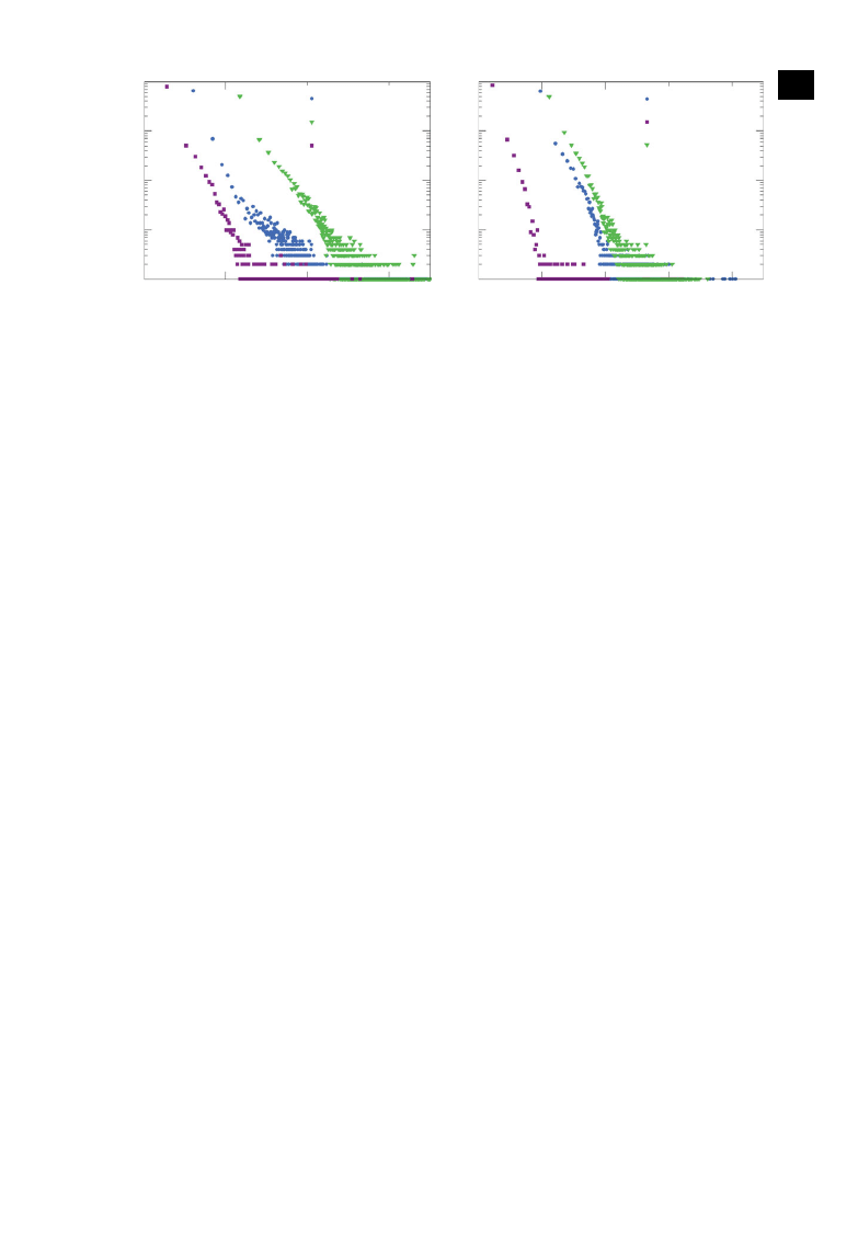
Figure 1. Energy distributions for (a) ER random and (b) BA scale-free networks. Each distribution is obtained from an ensemble of
10 000 networks. For most networks in the ensemble, the control energies diverge for values of the probability P
b
or the average degree
k larger than the ones shown in the figure. The initial states x
0
and the final states x
t
f
are randomly chosen, with the control time set
to t
f
= 1.
the required control energy is enormous and tends to diverge. For the cases where the energy can be
reasonably computed, it follows an algebraic distribution with fat tails, as shown in
with the
scaling exponent of about 1.5, regardless of the network type and size.
2.2. Structural determinants of control energy and energy distribution
We develop a physical understanding of the large control energy required and also the algebraic
scaling behaviour in the energy distribution. To gain insights, we first consider a simple model: a
unidirectional, one-dimensional string network, for which an analytic estimate of the control energy
can be obtained [
] as
E
l
≈ λ
−1
H
l
,
(2.4)
where l is the chain length (the number of nodes on the string) and
λ
H
l
is the smallest eigenvalue of
the underlying H-matrix, denoted by H
l
, which is related to the Gramian matrix by H
≡ e
−At
f
We
−A
T
t
f
.
Numerical verification of equation (
) is presented in
) is obtained
for a simple one-dimensional chain network, we find numerically and analytically that it also holds for
random and scale-free network topologies.
A brief derivation of equation (2.4) is as follows. The control energy required by the system can be
expressed as [
E(t
f
)
= x
T
0
· H
−1
· x
0
,
(2.5)
where x
0
is the initial state of the system. The matrix H is positive definite and symmetric with its inverse
satisfying H
−1
= QΛQ
T
, where
Λ and Q are the corresponding eigenvalue and eigenvector matrices,
respectively. Thus,
λ
−1
H
is the largest eigenvalue of H
−1
with
λ
H
denoting the smallest eigenvalue of H.
Numerically, we find that
λ
−1
H
is dramatically larger than any other eigenvalue. We have
E(t
f
)
= x
T
0
Q
ΛQ
T
x
0
=
N
i
=1
λ
i
(q
T
i
· x
0
)
2
≈ λ
−1
H
(q
T
1
· x
0
)
2
,
(2.6)
where q
i
is the ith column of Q. If the initial state x
0
is chosen to satisfy q
T
1
· x
0
= 1, we obtain E(t
f
)
≈ λ
−1
H
.
We find numerically that a random choice of x
0
does not change E(t
f
)’s order of magnitude. A detailed
derivation can be found in [
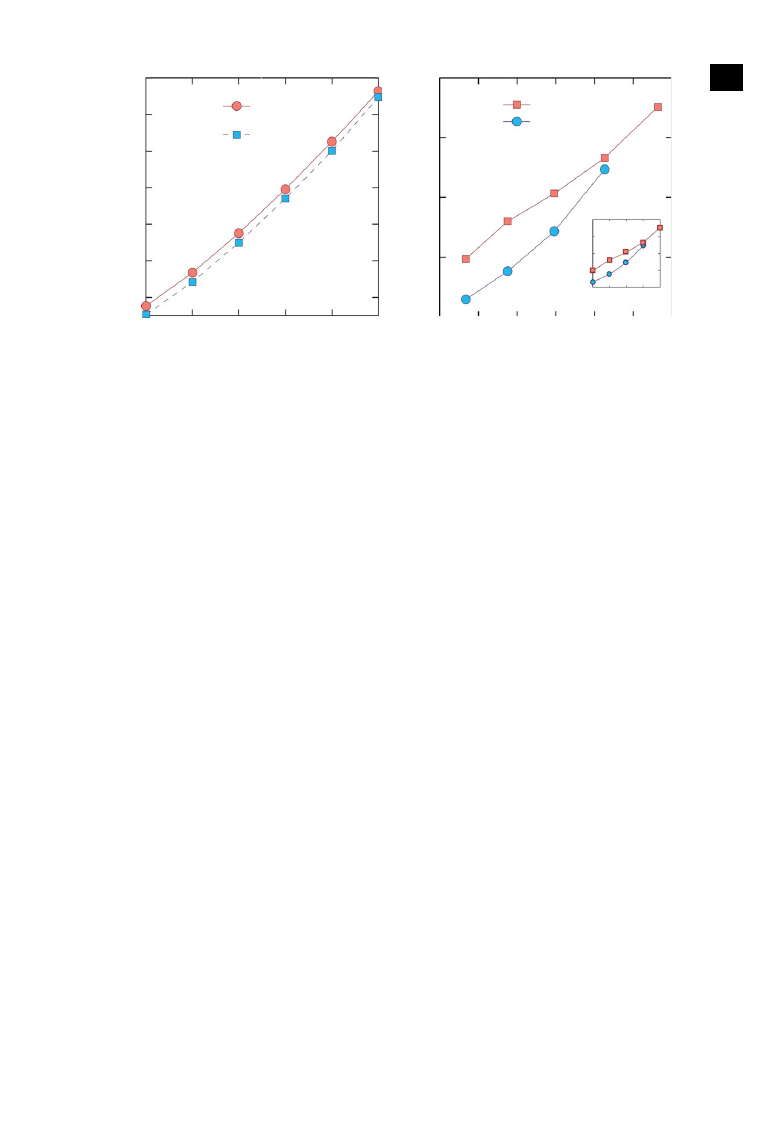
We see from
a, that the energy required for control tends to increase exponentially with the
chain length, indicating that even for a simple one-dimensional chain network of limited length, such as
l
= 7, the required control energy can be unbearably large. The exponential behaviour holds for complex
networks as well, as shown in the inset of
b for ER random and BA scale-free networks. In fact,
b indicates a strong positive correlation between the average control energy for the network and
E
L
, the energy required to control the LCC (to be described below) embedded in the network.
4
rsos
.ro
yalsociet
ypublishing
.or
g
R.
Soc
.open
sc
i.
3:
160064
................................................
10
14
10
13
10
11
10
9
10
7
10
5
10
2
10
4
10
13
10
11
10
9
10
7
10
5
3
4
5
6
7
10
6
10
8
10
10
10
12
10
14
10
12
10
10
10
8
10
6
10
4
10
2
2
3
4
5
l
E
L
L
E
l
l
H
l
E
l
·EÒ
6
7
–l
ER
BA
(a)
(b)
Figure 2. (a) For a one-dimensional chain network of length l, energy E
l
and
λ
−1
H
l
versus l. (b) Correlation between
E, the average
of control energy for networks with the same LCC length, and E
L
, the energy of an LCC of length D
C
= L (L = 3, 4, 5, 6 and 7 for ER and
L
= 3, 4, 5 and 6 for BA networks), calculated from ensembles of 10 000 networks. The inset in (b) shows the corresponding E versus
the LCC length L for BA and ER networks.
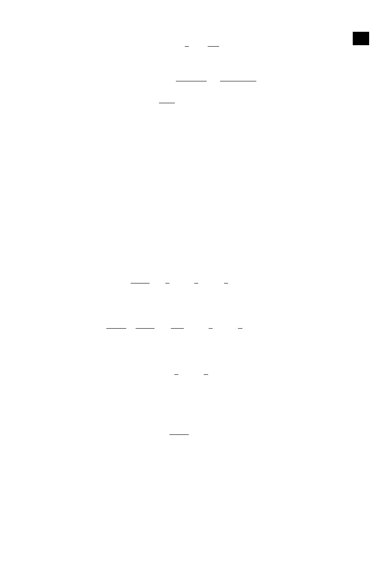
2.3. Concepts of control signal paths and longest control chains
In a networked system, control signal and energy originated from the driver nodes travel through one-
dimensional-string-like paths towards each of the non-driver nodes. As discussed, identifying maximum
matching so that the network is deemed structurally controllable does not guarantee convergent control
energy. When maximum matching is found, one can divide the whole network into N
D
CSPs, namely,
N
D
stems [
], each being a unidirectional one-dimensional string led by a driver node that passes
the control signal onto every node along the path, illustrated as the vertical paths in
. CSPs thus
provide a picture indicating how the signals from the N
D
external control inputs reach every node in the
network to ensure full control (in the sense of structural controllability).
How does the control energy flow through the network? To address this question, we distinguish two
types of links: one along and another between the CSPs, as shown in
. It may seem that the latter
links are less important as the control signal propagates along the former set of links. However, owing
to coupling, a node’s dynamical state will affect all its nearest neighbours’ states which, in turn, will
affect the states of their neighbours, and so on. In principle, any driver node is connected with nodes
both along and outside its CSP. Correspondingly, an arbitrary node in the network is influenced by every
driver node, directly through the CSP to which it belongs, or indirectly through the CSPs that it does
not sit on. Intuitively, the ability of a driver node to influence a node becomes weaker as the distance
between them is increased. In order to control a distant node, exponentially increased energy from the
driver is needed. The chain starting from a driver node and ending at a non-driver node along their
shortest path is effectively a control chain. Intuitively, control energy flows through the control chains,
while the control signal is propagated along the CSPs. We define the length of the longest control chain
(LCC), D
C
, as the control diameter of the network, as shown in
To find the LCCs in a network, we first use the maximum matching algorithm to find all the driver
nodes. We then identify the shortest paths from each of the driver nodes to each of the non-driver nodes.
Finally, we pick out the longest such shortest paths as LCCs. The computational complexity of finding the
LCCs are that associated with the maximum matching algorithm plus searching for the longest shortest
paths, which is feasible for large networks. There can be multiple LCCs. The node at the end of an LCC
is most difficult to be controlled in the sense that the largest amount of control energy is required. The
number m of such end nodes dictates the degeneracy (multiplicity) of LCCs. An example is shown in
, where we see that, although there are multiple LCCs, their ends converge to only three nodes,
leading to m
= 3. Since the energy required to control a one-dimensional chain grows exponentially with
its length in such a way that even one unit of increase in the length can amplify the energy by orders of
magnitude (
a), the energy associated with any chain shorter than the LCC can typically be several
orders of magnitude smaller than that with the LCC. Thus, the total energy is dominated by the LCCs.
5
rsos
.ro
yalsociet
ypublishing
.or
g
R.
Soc
.open
sc
i.
3:
160064
................................................
a
b
c
d
e
f
g
h
i
driver node:
non-driver node:
CSP link:
non-CSP link:
LCC:
LCC end-node
all possible LCCs:
c1
Æ
d3
Æ
e5
Æ
e6
i1
Æ
d3
Æ
e5
Æ
e6
i1
Æ
h2
Æ
e3
Æ
f5
c1
Æ
f3
Æ
f4
Æ
f5
e1
Æ
e2
Æ
e3
Æ
f5
e1
Æ
f3
Æ
f4
Æ
f5
c1
Æ
d3
Æ
e5
Æ
f6
i1
Æ
d3
Æ
e4
Æ
f6
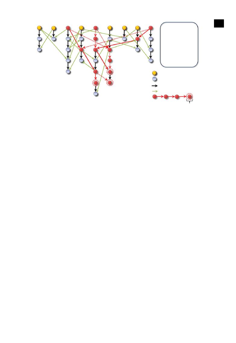
Figure 3. Schematic of CSPs (stems) and LCCs of a network. There are N
D
= 9CSPs,whicharealignedverticallyandlabelledasatoi.CSP
(or non-CSP) links are displayed in black (or green). In this example, the length of the LCCs is 4. Typically, a control chain may contain nodes
belonging to multiple CSPs. Two LCCs sharing no common nodes are marked by the red nodes and the solid red arrows. Links belonging
to other LCCs are marked by red dashed arrows. Each node is specified using its CSP label and its position along the CSP sequentially from
top to bottom. Eight LCCs in the network converge to only three end-nodes, e6, f 5 and f 6 (marked by red dashed circles), leading to LCC
degeneracy m
= 3. Note that the stems [
] (or CSPs) are originated from the driver nodes and are obtained through maximal matching.
Owing to the typically low value of m, a single LCC essentially dictates the energy required to control
the whole chain system. This is true especially for networks with long LCCs. Intuitively, the probability
to form long LCCs is small. Accordingly, a longer LCC tends to have smaller value of degeneracy m.
As a result, the longest LCCs have almost no degeneracy (m
= 1) so that they effectively rule the control
energy of the whole network.
In the structural controllability theory, a network is deemed more structurally controllable if N
D
is
smaller [
]. However, as the number of driver nodes is reduced, the length of the chain of nodes that
each controller drives on average must increase, leading to an increase in the LLC length and accordingly
an exponential growth in the control energy. In the ‘optimal’ case of structural controllability of N
D
= 1,
the LLC length will be maximized, leading to unrealistically large control energy that prevents us from
achieving actual control of the system.
Taken together, with respect to the previously defined concept of stem [
], we emphasize that a
stem is a path that propagates control signal from the input in the absence of a feedback loop (or a circle),
and each such path is determined by maximum matching, which allows a node to control at most one of
its immediate neighbours. Thus, a stem is in fact a CSP, which is quite different from the concept of an
LCC. Particularly, for a driver node and a non-driver node, a control chain is the shortest path between
them. For a set of driver nodes and all non-driver nodes in the entire network, an LCC is simply the
longest control chain. While control signals propagate through the CSPs, the energy may not flow along
the same paths due to the interactions among the nearest neighbours via the physical connections. For
example, the state change of a node can lead to state changes of all its nearest neighbours through the
energy exchange between this node and all its neighbours. That is, control energy flows through the
LCCs, not CSPs.
2.4. Control energy reduction scheme
Our finding of the LCC skeleton suggests a method to significantly reduce the control energy. A
straightforward solution is to break the LCCs with redundant controllers beyond those obtained via
maximum matching along the LCCs. Adding a redundant control input at the ith node of a unidirectional
one-dimensional chain of length l breaks it into two shorter sub-chains of length i
− 1 and l − i + 1.
Roughly, the control energy is the sum of energies required to control the two shorter components,
which is dominated by energy associated with the longer one owing to the exponential dependence
of the energy on the chain length. For i
≈ l/2, the length of the longer part is minimized. In simulations,
6
rsos
.ro
yalsociet
ypublishing
.or
g
R.
Soc
.open
sc
i.
3:
160064
................................................
0
0.5
1.0
0
0.5
1.0
College Student
Prison Inmate
s208a
s420a
s838a
Small World
Kohonen
Protein-1
Protein-2
Protein-3
St.martin
Seagrass
Grassland
Ythan
Silwood
Little Rock
Baydry
DE
*
mid
/E
*
n
D
n*
D
DE
*
R-mid
/E
*
(b)
(a)
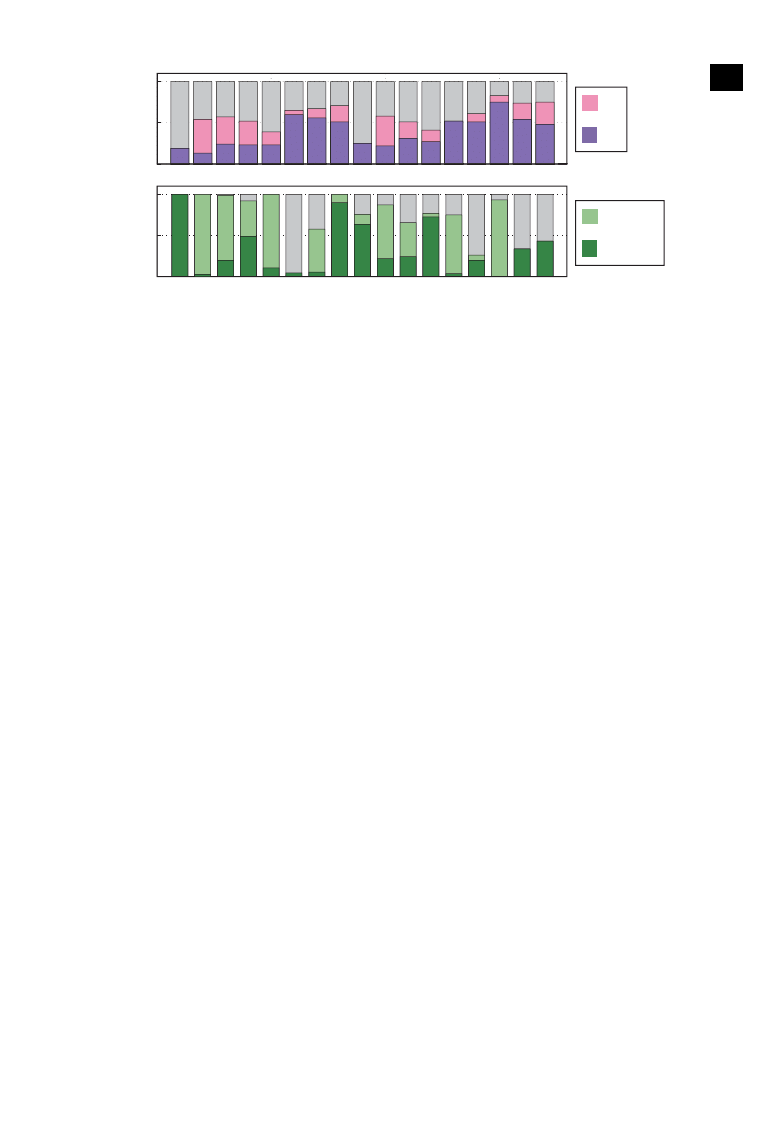
Figure 4. For the 17 real-world networks studied in [
], (a) densities of the original driver nodes n
D
(dark purple) and of the augmented
controls n
D
(light purple). (b) Normalized energy reduction
E
mid
/E
= (E
− E
mid
)
/E
(light green) when an additional control signal
is added to the middle of each LCC and normalized energy reduction
E
R
-
mid
/E
= (E
− E
R
-
mid
)
/E
(dark green) for the case where
the same number of control signals are randomly added into each network. All coloured bars start from 0. For the ‘Silwood’ network, the
energy with randomly added control signals is higher than the corresponding E
(the negative
E
R
-
mid
is not shown in the figure). For
the light green bars, the reduced control energy E
mid
is several orders of magnitude smaller than E
. The bars with more gray portion
than the light green potions are for the networks with relatively low values of E
and D
C
, for which energy reduction is not necessary.
applying a single redundant control input presents an extremely efficient energy reduction strategy for
one-dimensional chains: several orders of magnitude of reduction in the energy can be achieved. As a
realistic physical example, we considered a bidirectional cascading parallel R-C circuit of seven units,
which is effectively a one-dimensional chain of seven nodes with a self-loop at each node. For this
system, the redundant control input can be realized by inducing external current input into a capacitor.
A reduction in the joule energy of nearly 10 orders of magnitude is achieved [
For a complex network, the strategy of adding a redundant control at the middle of each LCC
dramatically outperforms the strategy of randomly adding an identical number of control inputs.
Treating the amount of the normalized energy reduction
E/E as a random variable across the ensemble
of networks, we obtain a monotonously increasing distribution function P(
E/E), reflecting the effect
of energy reduction. We find that high (low)
E/E values are more (less) probable under LCC-breaking
strategy when compared with the random strategy. For networks with longer LCCs, the strategy works
more effectively. For example, for networks with D
C
= 5, nearly 40% of the networks reach E/E ≈ 1,
but the same reduction can be achieved only for 2% of the networks via the random strategy.
For a large number of real-world networks, the mathematical structural controllability theory
stipulates that some of them are controllable with a few driving signals [
]. We find that most of these
networks (15 out of 17) require unrealistically high energies due mainly to their long LCCs. Strikingly,
even with unlimited energy supply, the number of driver nodes as determined by the maximum
matching algorithm is generally insufficient to fully control the whole system, where there exists a
number M
of nodes that never converge to their target states. These observations lead to the speculation
that, in order to fully control a realistic network, significantly more driver nodes are needed than those
identified by maximum matching. For example, N
D
= N
D
+ M
driver nodes should be deployed to
gain full control of the system, as shown in
a for n
D
and n
D
= N
D
/N for the 17 real-world
networks. Our energy reduction strategy is remarkably effective on the real-world networks with large
LCCs, as shown in
b. The quantity E
mid
is the control energy of a real-world network when a
redundant control input is applied at the middle of each LCC, while E
R-mid
denotes the energy when
the same number of redundant control inputs are randomly applied to the network. For each of the real-
world networks with unrealistically large energy requirement, the reduced control energy E
mid
is several
orders of magnitude lower than the original energy E
—the control energy with M
augmented driver
nodes without any LCC-breaking control input. The energy reduction due to random control signal

7
rsos
.ro
yalsociet
ypublishing
.or
g
R.
Soc
.open
sc
i.
3:
160064
................................................
augmentation is again much less effective in most cases, giving further evidence that the control energy
of real-world networks is generally determined by their LCCs.
To the best of our knowledge, the failure to converge to the target state with limitless energy
supply has not been observed for any modelled networks: it only occurs in empirical (real-world)
networks. It may be caused by some atypical structural properties. For example, for some networks,
the uncontrollable nodes form self-loops but without any incoming links. For some other networks with
an unusually high average degree, an ill-conditioned Gramian matrix can arise, prohibiting the system
from converging to the target state. However, such uncontrollable cases (even with infinite supply of
energy) are not expected to be generic.
3. Discussion
We fill a significant knowledge gap in the extremely active field of controlling complex networks by
developing a physical understanding of the recently discovered phenomena of algebraic distribution
and divergence of the required control energy. This is achieved through identification of LCCs,
the fundamental structure embedded in the network that dominantly determines the energy. The
understanding leads naturally to an optimization strategy to significantly reduce the control energy in
real-world networks: increasing the number of controllers slightly by placing redundant control signals
(beyond the number determined by the structural-controllability theory) along the LCCs. At present, the
issue of control energy can be addressed only in the linear controllability framework, but we believe that
the LCCs, due to their structural origin, can find counterparts in formulating theories of controllability
and observability for nonlinear dynamical networks [
], a largely open problem deserving much
attention and great research effort.
Our results that the LCCs essentially determine the network control energy are consistent with the
finding in [
]. In particular, for a one-dimensional unidirectional chain with exactly one control input, its
control energy has the standard definition that leads to the mathematical conclusion of energy divergence
for long chains, while the finding that anisotropic networks can be readily controlled was not obtained
under exactly the same setting. The dependence of a network’s control energy on its LCCs can be
further demonstrated via our energy reduction schemes, effective for both modelled and real-world
complex networks.
4. Methods
4.1. Longest control chain and control energy distribution
The construction illustrated in
provides a structural profile to estimate the control energy. In
particular, a network can be viewed as consisting of a set of control chains, and the total energy E required
has two components: E
(1)
, the sum of energies associated with all control chains, and E
(2)
, the interaction
energies among the chains, defined as E
− E
(1)
. The control chains are approximately independent of each
other so that E
(2)
is negligible as compared with E
(1)
. Each control chain is effectively a one-dimensional
string. Owing to the exponential increase in the energy with the chain length, E
(1)
can be regarded as the
sum of control energies associated with the set of LCCs. The required energy to control the full network
can thus be approximated as
E
= E
(1)
+ E
(2)
≈ E
(1)
≈ m · E
D
C
,
(4.1)
where E
D
C
denotes the energy required to control an LCC of length D
C
, and m denotes its degeneracy
(multiplicity), as shown in
. Reasoning from an alternative standpoint, an arbitrary combination
of D
C
and m, which we call an LCC skeleton, effectively represents a network, and the entire network
ensemble is equivalent to all the possible LCC skeletons according to a joint probability function
P(D
C
, m). The energy distribution for the original network can be characterized by the distribution of
the energy required to control the LCC skeleton in the ensemble. Through simulations, we find that the
marginal distribution of D
C
, P
D
C
(D
C
), decays approximately exponentially:
P
D
C
(D
C
)
= a · e
−b·D
C
,
(4.2)
where a and b are positive constants. Using
E
D
C
≈ A · e
B
·D
C
,
(4.3)
8
rsos
.ro
yalsociet
ypublishing
.or
g
R.
Soc
.open
sc
i.
3:
160064
................................................
we obtain
D
C
≈
1
B
ln
E
D
C
A
,
(4.4)
where A and B are positive constants, and consequently the distribution of E
D
C
as
P(E
D
C
)
= P
D
C
ln (E
D
C
/A)
B
·
d ln (E
D
C
/A)
dE
D
C
≈
aA
b
/B
B
· E
−(1+b/B)
D
C
.
(4.5)
The marginal distribution of m for networks with D
C
> 2 also exhibits an exponential decay:
P
m
(m)
= c · e
−g·m
,
(4.6)
where c and g are positive constants. Note that D
C
and m are uncorrelated, since a positive correlation
would imply that the number of LCCs increases with their length, which is unphysical, and a negative
correlation would lead to an exponential divergence of either P
D
C
(D
C
) or P
m
(m). We thus have
P(D
C
, m)
≈ P
D
C
(D
C
)
· P
m
(m)
(4.7)
and
P(E
D
C
, m)
≈ P
D
C
(E
D
C
)
· P
m
(m).
(4.8)
As a result, we obtain the following cumulative energy distribution:
F
E
(E)
= P(m · E
D
C
< E) =
∞
0
E
/E
DC
0
P(E
D
C
, m)
· dm
dE
D
C
=
∞
0
E
/E
DC
0
P
D
C
(E
D
C
)
· P
m
(m)
· dm
dE
D
C
≈
caA
b
/B
gB
·
−
b
B
−
Γ
b
B
− Γ
b
B
, gE
· (gE)
−b/B
,
(4.9)
where
Γ (b/B) and Γ (b/B, gE) are the Gamma and incomplete Gamma functions, respectively. The
distribution of E can then be expressed as
P
E
(E)
=
dF
E
(E)
dE
≈
caA
b
/B
gB
·
−
e
−gE
E
+
Γ
b
B
− Γ
b
B
, gE
· (gE)
−(1+b/B)
,
(4.10)
where
−e
−gE
/E ≈ 0 due to the typically large value of E. Since numerically the difference between the
two Gamma functions is approximately constant:
h
Γ
≡ Γ
b
B
− Γ
b
B
, gE
≈ 1.7,
(4.11)
P
E
(E) can be simplified as
P
E
(E)
≈ C · E
−(1+b/B)
,
(4.12)
providing a theoretical explanation for the algebraic energy distribution, where
C
=
caA
b
/B
gB
· g
−(2+b/B)
· h
Γ
is a positive constant. Numerically, we have B
≈ 2 and b ≈ 1. Accordingly, the theoretical estimate of
the scaling exponent is 1
+ b/B ≈ 1.5, which is consistent with the numerical value. The nearly identical
exponent in the distribution of E
D
C
indicates that the role of the LCC degeneracy m is insignificant in
the control energy and its distribution. It is the combination of the exponential decay in the distribution
of the control diameter and the exponential increase in the energy required to control LCCs with their
length which gives rise to the power-law energy distribution of the LCCs and ultimately leads to the
algebraic distribution in the actual energy required to control the original network.
We remark that, since the probability P
m
(m) has an exponential dependence on m and does not
explicitly contain the energy E
D
C
, the summation in m from 1 to E
/E
D
C
is a finite geometric sum, which
differs from the integral in only a constant coefficient and does not affect the algebraic scaling exponent
1
+ b/B. In our analysis, the reason to treat m as a real valued number is that the relation E ≈ mE
D
C
holds
9
rsos
.ro
yalsociet
ypublishing
.or
g
R.
Soc
.open
sc
i.
3:
160064
................................................
(b)
(a)
10
7
10
8
10
9
10
10
10
11
10
12
10
13
10
–1
10
–2
10
–3
10
–4
1
E
d
10
7
10
8
10
9
10
10
10
11
10
12
10
13
E
d
P
(E
d
)
10
–1
10
–2
10
–3
10
–4
1
D
C
= 5
D
C
= 6
random D
C
double-LCC interaction:
LCC-non-LCC interaction:
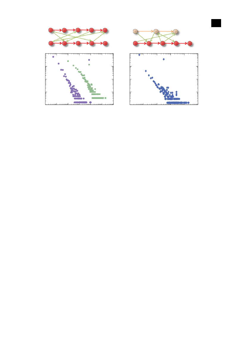
Figure 5. Distribution of control energy in a double-chain interaction models. (a) Two chains of D
C
= 5 and D
C
= 6, where the upper
panel is a schematic of two LCCs of identical length D
C
= 5 interacting with each other via some random links between them. (b) Two
chains with their lengths randomly chosen from 3 to 6, where the upper panel shows the case of two interacting chains of length 5
and 3. The longer chain plays the role of LCC, while the shorter chain is a non-LCC.
only in the order-of-magnitude sense, implying that E
/E
D
C
is typically not an integer. The limits m
→ 0
and E
D
C
→ ∞ correspond to the rare case where all nodes in the network belong to one single LCC.
If we treat m (1
≤ m ≤ E/E
D
C
) as an integer and accordingly set the integral upper bound of E
D
C
as E,
the cumulative energy distribution function will have a similar form to equation (4.9) with only a small
difference in the constant coefficient. This would not have any significant effect on the probability density
function P
E
(E) in equation (4.12). Numerically, E is typically a large number in the order of at least 10
10
.
As a result, the numerical difference caused by the integral upper bound is negligible.
4.2. Double-chain interaction
Our analysis of the LCC-skeleton predicts power-law distribution of the required energy for practically
controllable networks, which agrees qualitatively with numerics. However, interaction energy E
(2)
among the coexisting chains is ignored. In a physical system, interactions among the basic components
can play an important role in determining the system’s properties. To obtain a more accurate estimate
of the behaviours of the control energy, we need to include the interactions among the chains. The
necessity is further justified as there are discrepancies between the actual control energy and that from the
LCC-skeleton, as exemplified in
b. Thus, in order to reproduce the numerically obtained energy
distributions, we must incorporate the interactions among the LCCs into the model. However, including
the interactions makes analysis difficult, as there are typically a large number of interacting pairs of
chains. To gain insight into the role played by the interactions, it is useful to focus on the relatively
simple case of two interacting chains.
Our double-chain interaction model is constructed, as follows. Consider two identical unidirectional
chains, denoted by C1 and C2, each of length D
C
. Every node in C1 connects with every node in C2
with probability p, all links between the two chains are unidirectional. A link points to C2 from C1 with
probability p
1
→2
and the probability for a link in the opposite direction is p
2
→1
= 1 − p
1
→2
. By changing
the connection rate p and the directional bias p
1
→2
, we can simulate and characterize various interaction
patterns between the two chains. To be concrete, we generate an ensemble of 10 000 interacting double-
chain networks, each with 2
· D
C
nodes and multiple randomized inter-chain links as determined by
the parameters p and p
1
→2
. As shown in
a, the distribution of the control energy displays a
remarkable similarity to that for random networks, in that a power-law scaling behaviour emerges
with the exponent about 1.5. The power-law distribution holds robustly with respect to variations in
the parameters p and p
1
→2
, and the change in the magnitude of the energy due to small variations in

10
rsos
.ro
yalsociet
ypublishing
.or
g
R.
Soc
.open
sc
i.
3:
160064
................................................
the parameter values is insignificant when compared with that caused by a change in the length of the
LCC. In addition, to reveal the role of the interaction between an LCC and a non-LCC chain in the
control energy, we randomly pick their lengths from [
] with equal probability, where the longer chain
acts as an LCC. Again, we observe a strong similarity between the energy distributions from random
networks and from this model, as shown in
b, suggesting a universal pattern followed by pair
interactions, regardless of the length of the chains. In particular, interactions between two chains, LCC or
not, have a similar effect on the control-energy distribution. These results indicate that the double-chain
interaction model captures the essential physical ingredients of the energy distribution in controlling
complex networks.
Authors’ contributions.
Y.C.L. devised the research project. Y.Z.C. and L.Z.W. performed numerical simulations. Y.Z.C.,
L.Z.W., W.X.W. and Y.C.L. analysed the results. Y.Z.C. and Y.C.L. wrote the paper. All authors gave final approval
for publication.
Competing interests.
The authors declare no competing financial interests.
Funding.
This work was supported by ARO under grant no. W911NF-14-1-0504.
References
1.
Strogatz SH. 2001 Exploring complex networks.
Nature 410, 268–276. (
2.
Albert R, Barabási AL. 2002 Statistical mechanics
of complex networks. Rev. Mod. Phys. 74, 47–97.
(
3.
Mendes JFF, Dorogovtsev SN, Ioffe AF. 2003
Evolution of networks: from biological nets to the
internet and the WWW, 1st edn. Oxford UK: Oxford
University Press.
4. Pastor-Satorras R, Vespignani A. 2004 Evolution and
structure of the internet: a statistical physics
approach, 1st edn. Cambridge UK: Cambridge
University Press.
5.
Barrat A, Barthélemy M, Vespignani A. 2008
Dynamical processes on complex networks, 1st edn.
Cambridge UK: Cambridge University Press.
6. Newman MEJ. 2010 Networks: an introduction,
1st edn. Oxford, UK: Oxford University Press.
7.
Lombardi A, Hörnquist M. 2007 Controllability
analysis of networks. Phys. Rev. E 75, 056110.
(
doi:10.1103/PhysRevE.75.056110
8. Liu B, Chu T, Wang L, Xie G. 2008 Controllability of a
leader-follower dynamic network with switching
topology. IEEE Trans. Automat. Contr. 53, 1009–1013.
(
9. Rahmani A, Ji M, Mesbahi M, Egerstedt M. 2009
Controllability of multi-agent systems from a
graph-theoretic perspective. SIAM J. Contr. Optim.
48, 162–186. (
10. Liu YY, Slotine JJ, Barabási AL. 2011 Controllability of
complex networks. Nature 473, 167–173.
(
11. Wang WX, Ni X, Lai YC, Grebogi C. 2011 Optimizing
controllability of complex networks by small
structural perturbations. Phys. Rev. E 85, 026115.
(
doi:10.1103/PhysRevE.85.026115
12. Nacher JC, Akutsu T. 2012 Dominating scale-free
networks with variable scaling exponent:
heterogeneous networks are not difficult to control.
New J. Phys. 14, 073005. (
13. Yan G, Ren J, Lai YC, Lai CH, Li B. 2012 Controlling
complex networks: How much energy is needed?
Phys. Rev. Lett. 108, 218703. (
14. Nepusz T, Vicsek T. 2012 Controlling edge dynamics
in complex networks. Nat. Phys. 8, 568–573.
(
15. Liu YY, Slotine JJ, Barabási AL. 2013 Observability of
complex systems. Proc. Natl Acad. Sci. USA 110,
2460–2465. (
16. Yuan ZZ, Zhao C, Di ZR, Wang WX, Lai YC. 2013 Exact
controllability of complex networks. Nat. Commun.
4, 2447. (
17. Menichetti G, Dall’Asta L, Bianconi G. 2014 Network
controllability is determined by the density of low
in-degree and out-degree nodes. Phys. Rev. Lett.
113, 078701. (
doi:10.1103/PhysRevLett.113.078701
18. Ruths J, Ruths D. 2014 Control profiles of complex
networks. Science 343, 1373–1376. (
19. Wuchty S. 2014 Controllability in protein interaction
networks. Proc. Natl Acad. Sci. USA 111, 7156–7160.
(
20. Yuan ZZ, Zhao C, Wang WX, Di ZR, Lai YC. 2014 Exact
controllability of multiplex networks. New J. Phys.
16, 103036. (
21. Whalen AJ, Brennan SN, Sauer TD, Schiff SJ. 2015
Observability and controllability of nonlinear
networks: the role of symmetry. Phys. Rev. X 5,
011005. (
22. Yan G, Tsekenis G, Barzel B, Slotine JJ, Liu YY,
Barabási AL. 2015 Spectrum of controlling and
observing complex networks. Nat. Phys. 11,
779–786. (
23. Chen YZ, Wang LZ, Wang WX, Lai YC. 2015 The
paradox of controlling complex networks: control
inputs versus energy requirement. (
24. Lin CT. 1974 Structural controllability. IEEE Trans.
Automat. Contr. 19, 201–208. (
25. Hopcroft JE, Karp RM. 1973 An n
5
/2
algorithm for
maximum matchings in bipartite graphs. SIAM J.
Comput. 2, 225–231. (
26. Zhou H, Ou-Yang ZC. 2003 Maximum matching on
random graphs. (
http://arxiv.org/abs/cond-mat/
27. Zdeborová L, Mézard M. 2006 The number of
matchings in random graphs. J. Stat. Mech. 2006,
P05003. (
doi:10.1088/1742-5468/2006/05/P05003
28. Hautus MLJ. 1969 Controllability and observability
conditions of linear autonomous systems. In
Nederlandse Academie van Wetenschappen. Series A:
Mathematical Sciences, vol. 72, pp. 443–448.
Amsterdam, The Netherlands: Elsevier.
29. Rugh WJ. 1996 Linear systems theory. Englewood
Cliffs, NJ: Prentice-Hall, Inc.
30. Erdős P, Rényi A. 1959 On random graphs, I. Publ.
Math. 6, 290–297.
31. Erdős P, Rényi A. 1960 On the evolution of random
graphs. Publ. Math. Inst. Hung. Acad. Sci. 5, 17–61.
32. Sorrentino F, di Bernardo M, Garofalo F, Chen G.
2007 Controllability of complex networks via
pinning. Phys. Rev. E 75, 046103. (
33. Lai YC. 2014 Controlling complex, nonlinear
dynamical networks. Nat. Sci. Rev. 1, 339–341.
(
34. Pasqualetti F, Zampieri S. 2014 On the controllability
of isotropic and anisotropic networks. In 53rd IEEE
Conf. on Decision and Control, pp. 607–612.
Los Angeles, CA: IEEE.
Document Outline
Wyszukiwarka
Podobne podstrony:
Mirlin Statistics of energy levels and eigenfunctions in disordered systems (PR326, p259, 2000)(124s
Epidemics and immunization in scale free networks
The energy consumption and economic costs of different vehicles used in transporting woodchips Włoch
Barron Late lateral energy fractions and the envelopment question in concert halls
synthetic reductions in clandestine amphetamine and methamphetamine laboratories a review forensic s
Cadmium and Other Metal Levels in Autopsy Samplesfrom a Cadmium Polluted Area and Non polluted Contr
Can we accelerate the improvement of energy efficiency in aircraft systems 2010 Energy Conversion an
Transient TLR Activation Restores Inflammatory Response and Ability To Control Pulmonary Bacterial I
How effective are energy efficiency and renewable energy in curbing CO2 emissions in the long run A
War In Heaven A Completely New And Revolutionary Conception of The Nature of Spiritual Reality by K
(Parenting) Anger and Aggression in Children Teaching Self Control
Epidemic dynamics and endemic states in complex networks
Immunization and epidemic dynamics in complex networks
Role of Antibodies in Controlling Viral Disease Lessons from Experiments of Nature and Gene Knockout
Degradable Polymers and Plastics in Landfill Sites
Estimation of Dietary Pb and Cd Intake from Pb and Cd in blood and urine
Aftershock Protect Yourself and Profit in the Next Global Financial Meltdown
General Government Expenditure and Revenue in 2005 tcm90 41888
A Guide to the Law and Courts in the Empire
więcej podobnych podstron