
BRICS
L
S
-96-6
T
.
Bra
¨un
er:
In
tr
od
u
ction
to
Lin
ear
Logic
BRICS
Basic Research in Computer Science
Introduction to Linear Logic
Torben Bra ¨uner
BRICS Lecture Series
LS-96-6
ISSN 1395-2048
December 1996

Copyright c
1996, BRICS, Department of Computer Science
University of Aarhus. All rights reserved.
Reproduction of all or part of this work
is permitted for educational or research use
on condition that this copyright notice is
included in any copy.
See back inner page for a list of recent publications in the BRICS
Lecture Series. Copies may be obtained by contacting:
BRICS
Department of Computer Science
University of Aarhus
Ny Munkegade, building 540
DK - 8000 Aarhus C
Denmark
Telephone: +45 8942 3360
Telefax:
+45 8942 3255
Internet:
BRICS@brics.dk
BRICS publications are in general accessible through World Wide
Web and anonymous FTP:
http://www.brics.dk/
ftp://ftp.brics.dk/
This document in subdirectory LS/96/6/

Introduction to Linear Logic
Torben Bra¨uner


Torben Bra¨
uner
BRICS
1
Department of Computer Science
University of Aarhus
Ny Munkegade
DK-8000 Aarhus C, Denmark
1
Basic Research In Computer Science,
Centre of the Danish National Research Foundation.


Preface
The main concern of this report is to give an introduction to Linear Logic.
For pedagogical purposes we shall also have a look at Classical Logic as well
as Intuitionistic Logic. Linear Logic was introduced by J.-Y. Girard in 1987
and it has attracted much attention from computer scientists, as it is a logical
way of coping with resources and resource control. The focus of this technical
report will be on proof-theory and computational interpretation of proofs,
that is, we will focus on the question of how to interpret proofs as programs
and reduction (cut-elimination) as evaluation. We first introduce Classical
Logic. This is the fundamental idea of the proofs-as-programs paradigm.
Cut-elimination for Classical Logic is highly non-deterministic; it is shown
how this can be remedied either by moving to Intuitionistic Logic or to Linear
Logic. In the case on Linear Logic we consider Intuitionistic Linear Logic as
well as Classical Linear Logic. Furthermore, we take a look at the Girard
Translation translating Intuitionistic Logic into Intuitionistic Linear Logic.
Also, we give a brief introduction to some concrete models of Intuitionistic
Linear Logic. No proofs will be given except that a proof of cut-elimination
for the multiplicative fragment of Classical Linear Logic is included in an
appendix.
Acknowledgements. Thanks for comments from the participants of the
BRICS Mini-course corresponding to this technical report. The proof-rules
are produced using Paul Taylor’s macros.
v

vi

Contents
Preface
v
1
Classical and Intuitionistic Logic
1
1.1
Classical Logic
. . . . . . . . . . . . . . . . . . . . . . . . . .
1
1.2
Intuitionistic Logic . . . . . . . . . . . . . . . . . . . . . . . .
5
1.3
The λ-Calculus . . . . . . . . . . . . . . . . . . . . . . . . . .
8
1.4
The Curry-Howard Isomorphism . . . . . . . . . . . . . . . . . 12
2
Linear Logic
14
2.1
Classical Linear Logic . . . . . . . . . . . . . . . . . . . . . . . 14
2.2
Intuitionistic Linear Logic . . . . . . . . . . . . . . . . . . . . 19
2.3
A Digression - Russell’s Paradox and Linear Logic . . . . . . . 23
2.4
The Linear λ-Calculus . . . . . . . . . . . . . . . . . . . . . . 27
2.5
The Curry-Howard Isomorphism . . . . . . . . . . . . . . . . . 31
2.6
The Girard Translation . . . . . . . . . . . . . . . . . . . . . . 32
2.7
Concrete Models
. . . . . . . . . . . . . . . . . . . . . . . . . 35
A Logics
40
A.1 Classical Logic
. . . . . . . . . . . . . . . . . . . . . . . . . . 40
A.2 Intuitionistic Logic . . . . . . . . . . . . . . . . . . . . . . . . 42
A.3 Classical Linear Logic . . . . . . . . . . . . . . . . . . . . . . . 43
A.4 Intuitionistic Linear Logic . . . . . . . . . . . . . . . . . . . . 45
B Cut-Elimination for Classical Linear Logic
46
B.1 Some Preliminary Results . . . . . . . . . . . . . . . . . . . . 46
B.2 Putting the Proof Together
. . . . . . . . . . . . . . . . . . . 52
vii

viii

Chapter 1
Classical and Intuitionistic
Logic
This chapter introduces Classical Logic and Intuitionistic Logic. Also, the
Curry-Howard interpretation of Intuitionistic Logic, the λ-calculus, is dealt
with.
1.1
Classical Logic
The presentation of Classical Logic given in this section is based on the book
[GLT89]. Formulas of Classical Logic are given by the grammar
s ::= 1
| s ∧ s | 0 | s ∨ s | s ⇒ s.
The meta-variables A, B, C range over formulae. Proof-rules for a Gentzen
style presentation of the logic are given in Appendix A.1; they are used to
derive sequents
A
1
, ..., A
n
` B
1
, ..., B
m
.
Such a sequent amounts to the formula expressing that the conjunction of
A
1
, ..., A
n
implies the disjunction of B
1
, ..., B
m
.
The meta-variables Γ, ∆
range over lists of formulae and π, τ range over derivations as well as proofs.
The Γ and ∆ parts of a sequent Γ
` ∆ are called contexts. The presence
of contraction and weakening proof-rules allows us to consider the contexts
of a sequent as sets of formulae rather than multisets of formulae, which is
1

Chapter 1.
Classical and Intuitionistic Logic
a feature distinguishing Classical Logic and Intuitionistic Logic from Linear
Logic. The Gentzen style proof-rules were originally introduced in [Gen34].
This presentation is characterised by the presence of two different forms of
rules for each connective, depending on which side of the turnstile the in-
volved connective is introduced. Note that in Appendix A.1 the rules that
introduce a connective on the left hand side have been positioned in the left
hand side column, and similarly, the rules that introduce a connective on the
right hand side have been positioned in the right hand side column. Note
also that the rules for conjunction are symmetric to those for disjunction.
In the system above, negation is defined as
¬A = A ⇒ 0. An alternative
formulation of Classical Logic can be obtained by leaving out implication
and having negation as a builtin connective together with the proof-rules
Γ
` A, ∆
¬
L
Γ,
¬A ` ∆
Γ, A
` ∆
¬
R
Γ
` ¬A, ∆
Implication is then defined as A
⇒ B = ¬A ∨ B. We would then have a
perfectly symmetric system. However, we have chosen the system of Ap-
pendix A.1 with the aim of making clear the connection to Intuitionistic
Logic.
One of the most important properties of the proof-rules for Classical Logic
is that the cut-rule is redundant; this was originally proved by Gentzen in
[Gen34]. The idea is that an application of the cut rule can either be pushed
upwards in the surrounding proof or it can be replaced by cuts involving
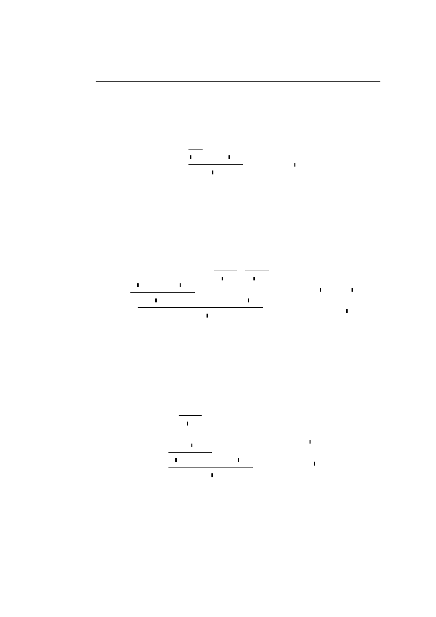
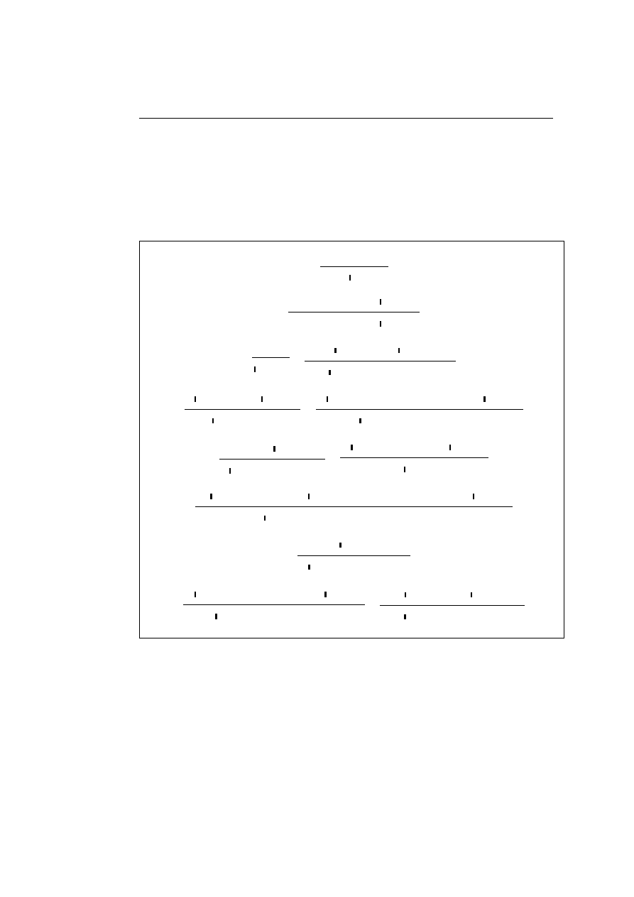
simpler formulae. The latter situation amounts to the following key-cases in
which the cut formula is introduced in the last used rules of both immediate
subproofs:
• The (∧
R
,
∧
L1
) key-case
··
· π
1
Γ
` A, ∆
··
· π
2
Γ
0
` B, ∆
0
Γ, Γ
0
` A ∧ B, ∆, ∆
0
··
· π
0
1
Γ
00
, A
` ∆
00
Γ
00
, A
∧ B ` ∆
00
Γ
00
, Γ, Γ
0
` ∆
00
, ∆, ∆
0
;
··
· π
1
Γ
` A, ∆
··
· π
0
1
Γ
00
, A
` ∆
00
Γ
00
, Γ
` ∆
00
, ∆
================
Γ
00
, Γ, Γ
0
` ∆
00
, ∆
0
, ∆
2

1.1.
Classical Logic
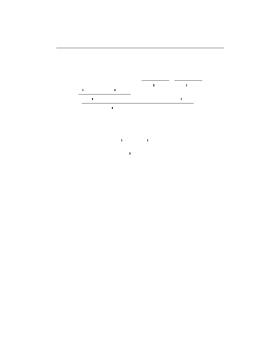
• The (∧
R
,
∧
L2
) key-case
··
·
π
1
Γ
` A, ∆
··
·
π
2
Γ
0
` B, ∆
0
Γ, Γ
0
` A ∧ B, ∆, ∆
0
··
·
π
0
1
Γ
00
, B
` ∆
00
Γ
00
, A
∧ B ` ∆
00
Γ
00
, Γ, Γ
0
` ∆
00
, ∆, ∆
0
;
··
·
π
2
Γ
0
` B, ∆
0
··
·
π
0
1
Γ
00
, B
` ∆
00
Γ
00
, Γ
0
` ∆
00
, ∆
0
================
Γ
00
, Γ, Γ
0
` ∆
00
, ∆
0
, ∆
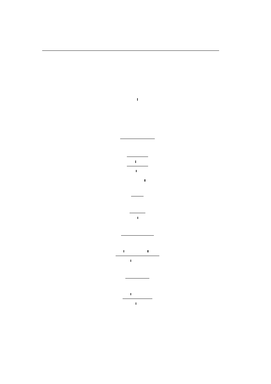
• The (1
R
, 1
L
) key-case
` 1
··
·
π
0
1
Γ
0
` ∆
0
Γ
0
, 1
` ∆
0
Γ
0
` ∆
0
;
··
· π
0
1
Γ
0
` ∆
0
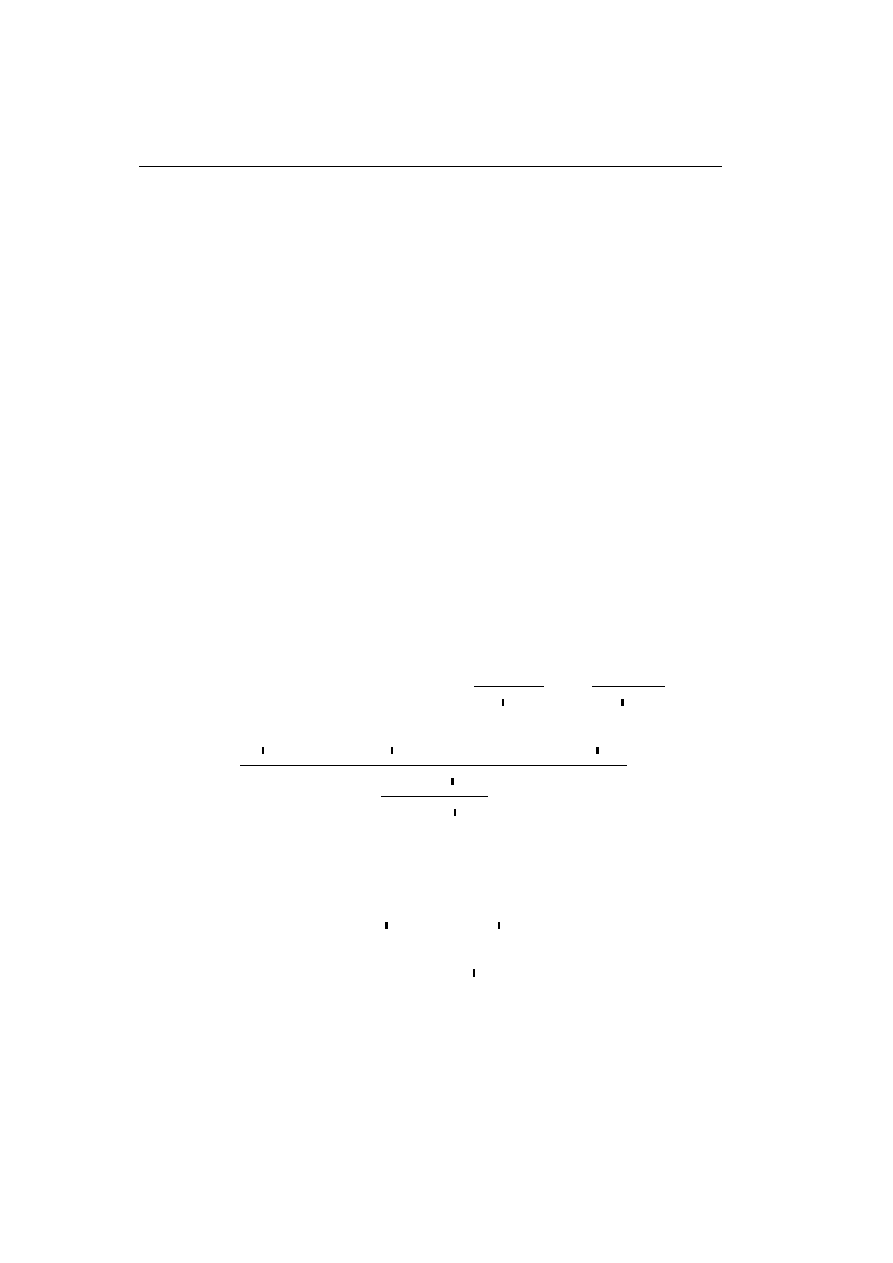
• The (⇒
R
,
⇒
L
) key-case
··
·
π
1
Γ, A
` B, ∆
Γ
` A ⇒ B, ∆
··
·
π
0
1
Γ
0
` A, ∆
0
··
·
π
0
2
Γ
00
, B
` ∆
00
Γ
0
, Γ
00
, A
⇒ B ` ∆
00
, ∆
0
Γ
0
, Γ
00
, Γ
` ∆
00
, ∆
0
, ∆
;
··
·
π
0
1
Γ
0
` A, ∆
0
··
· π
1
Γ, A
` B, ∆
··
· π
0
2
Γ
00
, B
` ∆
00
Γ
00
, Γ, A
` ∆
00
, ∆
Γ
00
, Γ, Γ
0
` ∆
00
, ∆, ∆
0
A double bar denotes a number of applications of rules.
We also have
(
∨
R1
,
∨
L
), (
∨
R2
,
∨
L
), and (0
R
, 0
L
) key-cases, but they are left out as they
3

Chapter 1.
Classical and Intuitionistic Logic
are symmetric to the mentioned (
∧
R
,
∧
L1
), (
∧
R
,
∧
L2
), and (1
R
, 1
L
) cases, re-
spectively. We omit the full cut-elimination proof here; the reader is referred
to [GLT89] for the details. A notable feature of the system is that all formu-
lae occuring in a cut-free proof are subformulae of the formulae occuring in
the end-sequent. This is called the subformula property.
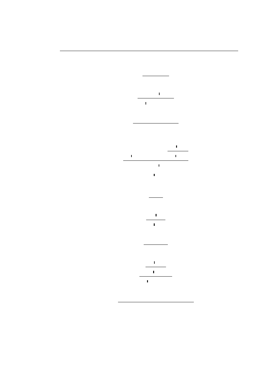
The fundamental idea in the proofs-as-programs paradigm is to consider
a proof as a program and reduction of the proof (cut-elimination) as evalua-
tion of the program. This makes it desirable that the same reduced proof is
obtained independent of the choices of reductions. However, this is not pos-
sible with Classical Logic where cut-elimination is highly non-deterministic,
as pointed out in [GLT89]. The problem is witnessed by the proof
··
·
π
Γ
` ∆
Γ
` A, ∆
··
·
π
0
Γ
0
` ∆
0
Γ
0
, A
` ∆
0
Γ
0
, Γ
` ∆
0
, ∆
which, because of its symmetry, can be reduced to both of the proofs
··
·
π
Γ
` ∆
==========
Γ
0
, Γ
` ∆
0
, ∆
··
· π
0
Γ
0
` ∆
0
==========
Γ
0
, Γ
` ∆
0
, ∆
The example implies that Classical Logic as given above has no non-trivial
sound denotational semantics; all proofs of a given sequent will simply have
the same denotation. This deficiency can be remedied by breaking the sym-
metry; two ways of doing so can be pointed out:
• Each right hand side context is subject to the restriction that it has
to contain exactly one formula. This amounts to Intuitionistic Logic
which will be dealt with in Section 1.2.
• Contraction and weakening is marked explicitly using additional modal-
ities ! and ? on formulae. The !-modality corresponds to contraction
and weakening on the left hand side, and similarly, the ?-modality cor-
responds to contraction and weakening on the right hand side. This
amounts to Classical Linear Logic which will be dealt with in Sec-
tion 2.1.
4

1.2.
Intuitionistic Logic
This dichotomy goes back to [GLT89]. Since the publication of this book
a considerable amount of work has been devoted to giving Classical Logic
a constructive formulation in the sense that proofs can be considered as
programs. This has essentially been achieved by “decorating” formulas with
information controlling the process of cut-elimination. The work of Parigot,
[Par91, Par92], Ong, [Ong96] and Girard, [Gir91] seems especially promising.
A notable feature of the latter paper is the presentation of a categorical model
of Classical Logic where A is not isomorphic to
¬¬A. Thus, the dichotomy
above should not be considered as excluding other solutions. The lesson to
learn is that constructiveness, in the sense that proofs can be considered as
programs, is not a property of certain logics, but rather a property of certain
formulations of logics.
1.2
Intuitionistic Logic
The presentation of Intuitionistic Logic given in this section is based on the
book [GLT89]. Formulae of Intuitionistic Logic are the same as the formulae
of Classical Logic. The proof-rules of Intuitionistic Logic in Gentzen style
occur as those of Classical Logic given in Appendix A.1 where
∨
L
is written
Γ, A
` C Γ
0
, B
` C
∨
L
Γ, Γ
0
, A
∨ B ` C
and the remaining rules are subject to the restriction that each right hand
side context contains exactly one formula.
We shall here consider also an equivalent Natural Deduction presentation
of Intuitionistic Logic which has cleaner dynamic properties than the pre-
sentation in Gentzen style. Proof-rules for this formulation of the logic are
given in Appendix A.2; they are used to derive sequents
A
1
, ..., A
n
` B.
The Natural Deduction style proof-rules were originally introduced by Gentzen
in [Gen34] and later considered by Pravitz in [Pra65]. This style of presen-
tation is characterised by the presence of two different forms of rules for
each connective, namely introduction and elimination rules. Note that in
Appendix A.2 the introduction rules have been positioned in the left hand
5

Chapter 1.
Classical and Intuitionistic Logic
side column, and the elimination rules have been positioned in the right hand
side column. Note also that the contraction and weakening proof-rules are
explicitly part of the Gentzen style formulation whereas they are admissible
in the Natural Deduction formulation.
A notable feature of Intuitionistic Logic is the so-called Brouwer-Heyting-
Kolmogorov functional interpretation where formulae are interpreted by means
of their proofs:
• A proof of a conjunction A ∧ B consists of a proof of A together with
a proof of B,
• a proof of an implication A ⇒ B is a function from proofs of A to
proofs of B,
• a proof of a disjunction A ∨ B is either a proof of A or a proof of
B together with a specification of which of the disjuncts is actually
proved.
The proof-rules for Intuitionistic Logic can then be considered as methods for
defining functions such that a proof of a sequent Γ
` B gives rise to a function
which assigns a proof of the formula B to a list of proofs proving the respective
formulae in the context Γ. Note that tertium non datur, A
∨ ¬A, which
distinguishes Classical Logic from Intuitionistic Logic, cannot be interpreted
in this way. It turns out that the λ-calculus is an appropriate language for
expressing the Brouwer-Heyting-Kolmogorov interpretation. We shall come
back to the λ-calculus in the next section, and in Section 1.4 we will introduce
the Curry-Howard isomorphism that makes explicit the relation between the
λ-calculus and Intuitionistic Logic.
Now, a Natural Deduction proof may be rewritten into a simpler form
using a reduction rule. Reduction of a Natural Deduction proof corresponds
to cut-eliminating in a Gentzen style formulation. The reduction rules are
as follows:
6

1.2.
Intuitionistic Logic
• The (∧
I
,
∧
E1
) case
··
·
Γ
` A
··
·
Γ
` B
Γ
` A ∧ B
Γ
` A
;
··
·
Γ
` A
• The (∧
I
,
∧
E2
) case
··
·
Γ
` A
··
·
Γ
` B
Γ
` A ∧ B
Γ
` B
;
··
·
Γ
` B
• The (⇒
I
,
⇒
E
) case
Γ, A, Λ
` A
··
·
Γ, A
` B
Γ
` A ⇒ B
··
·
Γ
` A
Γ
` B
;
··
·
Γ, Λ
` A
··
·
Γ
` B
• The (∨
I1
,
∨
E
) case
··
·
Γ
` A
Γ
` A ∨ B
Γ, A, Λ
` A
··
·
Γ, A
` C
Γ, B, ∆
` B
··
·
Γ, B
` C
Γ
` C
;
··
·
Γ, Λ
` A
··
·
Γ
` C
7

Chapter 1.
Classical and Intuitionistic Logic
• The (∨
I2
,
∨
E
) case
··
·
Γ
` B
Γ
` A ∨ B
Γ, A, Λ
` A
··
·
Γ, A
` C
Γ, B, ∆
` B
··
·
Γ, B
` C
Γ
` C
;
··
·
Γ, ∆
` B
··
·
Γ
` C
Note how a reduction rule removes a “detour” in the proof created by the
introduction of a connective immediately followed by its elimination.
The Natural Deduction presentation of Intuitionistic Logic satisfies the
Church-Rosser property which means that whenever a proof π reduces to
π
0
as well as to π
00
, there exists a proof π
000
to which both of the proofs π
0
and π
00
reduce, and moreover, it satisfies the strong normalisation property
which means that all reduction sequences originating from a given proof are
of finite length. Church-Rosser and strong normalisation implies that any
proof π reduces to a unique proof with the property that no reductions can
be applied; this is called the normal form of π.
Via the Curry-Howard
isomorphism this corresponds to analogous results for reduction of terms of
the λ-calculus which we will come back to in the next two sections.
1.3
The λ-Calculus
The presentation of the λ-calculus given in this section is based on the book
[GLT89]. In the next section we shall see how the λ-calculus occurs as a
Curry-Howard interpretation of Intuitionistic Logic. Note that we consider
products and sums as part of the λ-calculus; this convention is not followed
by all authors. Types of the λ-calculus are given by the grammar
s ::= 1
| s × s | s ⇒ s | 0 | s + s
8

1.3.
The
λ-Calculus
Figure 1.1: Type Assignment Rules for the λ-Calculus
x
1
: A
1
, ..., x
n
: A
n
` x
q
: A
q
Γ
` true : 1
Γ
` u : A Γ ` v : B
Γ
` (u, v) : A × B
Γ
` u : A × B
Γ
` fst(u) : A
Γ
` u : A × B
Γ
` snd(u) : B
Γ, x : A
` u : B
Γ
` λx
A
.u : A
⇒ B
Γ
` f : A ⇒ B Γ ` u : A
Γ
` fu : B
Γ
` w : 0
Γ
` false
C
(w) : C
Γ
` u : A
Γ
` inl
A+B
(u) : A + B
Γ
` u : B
Γ
` inr
A+B
(u) : A + B
Γ
` w : A + B Γ, x : A ` u : C Γ, y : B ` v : C
Γ
` case w of inl(x).u
|
inr(y).v : C
and terms are given by the grammar
t ::=
x
|
true
| (t, t) | fst(t) | snd(t) |
λx
A
.t
| tt |
false
C
(t)
| inl
A+B
(t)
| inr
A+B
(t)
| case t of inl(x).t
|
inr(y).t
9

Chapter 1.
Classical and Intuitionistic Logic
where x is a variable ranging over terms. The set of free variables, denoted
F V (u), of a term u is defined by structural induction on u as follows:
F V (x) =
{x}
F V (true) =
∅
F V ((u, v)) = F V (u)
∪ F V (v)
F V (fst(u)) = F V (u)
F V (λx.u) = F V (u)
− {x}
F V (f u) = F V (f )
∪ F V (u)
F V (false(u)) = F V (u)
F V (inl(u)) = F V (u)
F V (case w of inl(x).u
|
inr(y).v) = F V (w)
∪F V (u)−{x}∪F V (v)−{y}
We say that a term u is closed iff F V (u) =
∅. We also say that the variable
x is bound in the term λx.u. A similar remark applies to the case construc-
tion. We need a convention dealing with substitution: If a term v together
with n terms u
1
, ..., u
n
and n pairwise distinct variables x
1
, ..., x
n
are given,
then v[u
1
, ..., u
n
/x
1
, ..., x
n
] denotes the term v where simultaneously the terms
u
1
, ..., u
n
have been substituted for free occurrences of the variables x
1
, ..., x
n
such that bound variables in v have been renamed to avoid capture of free
variables of the terms u
1
, ..., u
n
. Occasionally a list u
1
, ..., u
n
of n terms will
be denoted u and a list x
1
, ..., x
n
of n pairwise distinct variables will be de-
noted x. Given the definition of free variables above, it should be clear how
to formalise substitution.
Rules for assignment of types to terms are given in Figure 1.1. Type
assignments have the form of sequents
x
1
: A
1
, ..., x
n
: A
n
` u : B
where x
1
, ..., x
n
are pairwise distinct variables. It can be shown by induction
on the derivation of the type assignment that
F V (u)
⊆ {x
1
, ..., x
n
}.
The λ-calculus satisfies the following properties:
Lemma 1.3.1 If the sequent Γ
` u : A is derivable, then for any derivable
sequent Γ
` u : B we have A = B.
10

1.3.
The
λ-Calculus
Proof: Induction on the derivation of Γ
` u : A.
2
The following proposition is the essence of the Curry-Howard isomorphism:
Proposition 1.3.2 If the sequent Γ
` u : A is derivable, then the rule
instance above the sequent is uniquely determined.
Proof: Use Lemma 1.3.1 to check each case.
2
We need a small lemma dealing with expansion of contexts.
Lemma 1.3.3 If the sequent ∆, Λ
` u : A is derivable and the variables in
the contexts ∆, Λ and Γ are pairwise distinct, then the sequent ∆, Γ, Λ
` u : A
is also derivable.
Proof: Induction on the derivation of ∆, Λ
` u : A.
2
Now comes a lemma dealing with substitution.
Lemma 1.3.4 (Substitution Property) If both of the sequents Γ
` u : A
and Γ, x : A, Λ
` v : B are derivable, then the sequent Γ, Λ ` v[u/x] : B is
also derivable.
Proof: Induction on the derivation of Γ, x : A, Λ
` v : B. We need
Lemma 1.3.3 for the case where the derivation is an axiom
x
1
: A
1
, ..., x
n
: A
n
` x
q
: A
q
such that the variable x is equal to x
q
.
2
The λ-calculus has the following β-reduction rules each of which is the image
under the Curry-Howard isomorphism of a reduction on the proof corre-
sponding to the involved term:
fst((u, v))
;
u
snd((u, v))
;
v
(λx.u)w
;
u[w/x]
case inl(w) of inl(x).u
|
inr(y).v
;
u[w/x]
case inr(w) of inl(x).u
|
inr(y).v
;
v[w/y]
11

Chapter 1.
Classical and Intuitionistic Logic
We shall not be concerned with η-reductions or commuting conversions. The
properties of Church-Rosser and strong normalisation for proofs of Intuition-
istic Logic correspond to analogous notions for terms of the λ-calculus via
the Curry-Howard isomorphism, and in [LS86] it is shown that these prop-
erties are indeed satisfied. First strong normalisation is proved. By K¨
onig’s
Lemma, this implies that any term t is bounded , that is, there exists a number
n such that no sequence of one-step reductions originating from t has more
than n steps. Given the result that all terms are bounded, Church-Rosser is
proved by induction on the bound.
1.4
The Curry-Howard Isomorphism
The original Curry-Howard isomorphism, [How80], relates the Natural De-
duction formulation of Intuitionistic Logic to the λ-calculus; formulae cor-
respond to types, proofs to terms, and reduction of proofs to reduction of
terms. This is dealt with in [GLT89] and in [Abr90]; the first emphasises the
logic side of the isomorphism, the second the computational side. In what
follows, we will consider the Natural Deduction presentation of Intuitionistic
Logic given in Appendix A.2. The relation between formulae of Intuitionistic
Logic and types of the λ-calculus is obvious. The idea of the Curry-Howard
isomorphism on the level of proofs is that proof-rules can be “decorated”
with terms such that the term induced by a proof encodes the proof. In the
case of Intuitionistic Logic an appropriate term language for this purpose
is the λ-calculus. If we decorate the proof-rules of Intuitionistic Logic with
terms in the appropriate way we get the rules for assigning types to terms
of the λ-calculus, and moreover, if we take the typing rules of the λ-calculus
and remove the variables and terms we can recover the proof-rules. We get
the Curry-Howard isomorphism on the level of proofs as follows: Given a
proof of the sequent A
1
, ..., A
n
` B, that is, a proof of the formula B on as-
sumptions A
1
, ..., A
n
, one can inductively construct a derivation of a sequent
x
1
: A
1
, ..., x
n
: A
n
` u : B, that is, a term u of type B with free variables
x
1
, ..., x
1
of respective types A
1
, ..., A
n
. Conversely, if one has a derivable
sequent x
1
: A
1
, ..., x
n
: A
n
` u : B, there is an easy way of getting a proof
of A
1
, ..., A
n
` B; erase all terms and variables in the derivation of the type
assignment. The two processes are each other’s inverses modulo renaming
of variables. The isomorphism on the level of proofs is essentially given by
12

1.4.
The Curry-Howard Isomorphism
Proposition 1.3.2.
On the level of reduction the Curry-Howard isomorphism says that a re-
duction on a proof followed by application of the Curry-Howard isomorphism
on the level of proofs, yields the same term as application of the Curry-
Howard isomorphism on the level of proofs followed by the term-reduction
corresponding to the proof-reduction. This can be verified by applying the
Curry-Howard isomorphism to the proofs involved in the reduction rules of
Intuitionistic Logic. For example, in the case of a (
⇒
I
,
⇒
E
) reduction we
get
Γ, x : A, Λ
` x : A
··
·
Γ, x : A
` u : B
Γ
` λx.u : A ⇒ B
··
·
Γ
` v : A
Γ
` (λx.u)v : B
;
··
·
Γ, Λ
` v : A
··
·
Γ
` u[v/x] : B
We see that a β-reduction has taken place on the term encoding the proof
on which the reduction is performed. In fact all β-reductions appear as
Curry-Howard interpretations of reductions on the corresponding proofs.
13

Chapter 2
Linear Logic
This chapter introduces Classical Linear Logic and Intuitionistic Linear Logic.
We make a detour to Russell’s Paradox with the aim of illustrating the dif-
ference between Intuitionistic Logic and Intuitionistic Linear Logic. Also,
the Curry-Howard interpretation of Intuitionistic Linear Logic, the linear
λ-calculus, is dealt with. Furthermore, we take a look at the Girard Transla-
tion translating Intuitionistic Logic into Intuitionistic Linear Logic. Finally,
we give a brief introduction to some concrete models of Intuitionistic Linear
Logic.
2.1
Classical Linear Logic
Linear Logic was discovered by J.-Y. Girard in 1987 and published in the
now famous paper [Gir87]. In the abstract of this paper, it is stated that
“a completely new approach to the whole area between constructive logics
and computer science is initiated”. In [Gir89] the conceptual background of
Linear Logic is worked out. The fundamental idea of Linear Logic is to control
the use of resources which is witnessed by the fact that the contraction and
weakening proof-rules are not admissible in general. Rather, Linear Logic
occurs essentially as Classical Logic with the restriction that contraction
and weakening is marked explicitly using additional modalities ! and ? on
formulae. The !-modality corresponds to contraction and weakening on the
left hand side, and similarly, the ?-modality corresponds to contraction and
weakening on the right hand side. A proof of !A amounts to having a proof
14

2.1.
Classical Linear Logic
of A that can be used an arbitrary number of times.
Here we shall only consider the multiplicative fragment of Classical Linear
Logic. Formulae are given by the grammar
s ::= I
| s ⊗ s | ⊥ | s
.............................
......
..
............
...........
....
...
...
....
...........
..
........
s
| s ( s | !s | ?s | & | 1 | ⊕ | 0.
Proof-rules for a Gentzen style presentation of the logic are given in Ap-
pendix A.3; they are used to derive sequents
A
1
, ..., A
n
− B
1
, ..., B
m
.
A Girardian turnstile
− is used to distinguish sequents of Classical Linear
Logic from sequents of Classical Logic, where the usual turnstile
` is used.
The &,1,
⊕ and 0 connectives are called additive. The system obtained by
excluding the additives is called the multiplicative fragment. Note that, un-
like most presentations of Classical Linear Logic, we use two-sided sequents,
which will make the connection to Intuitionistic Linear Logic more explicit.
Negation is then defined as A
⊥
= A
(⊥. The absence of contraction and
weakening prevents us from considering the contexts of a sequent as sets of
formulae, but we have to consider them to be multisets instead. This should
be compared to Classical and Intuitionistic Logic where we do have contrac-
tion and weakening which implies that contexts can be considered as sets of
formulae. The fact that contexts are considered as multisets means that ev-
ery formula occuring in the context of a sequent has to be used exactly once.
Therefore the two conjunctions & and
⊗ of Linear Logic are very different
constructs: A proof of A&B consists of a proof of A together with a proof
of B where exactly one of the proofs has to be used. A proof of A
⊗ B also
consists of a proof of A together with a proof of B but here both of the proofs
have to be used.
Now, as with Classical Logic, the cut-rule of Classical Linear Logic is
redundant. Again the idea is that an application of the cut rule can either
be pushed upwards in the surrounding proof or it can be replaced by cuts
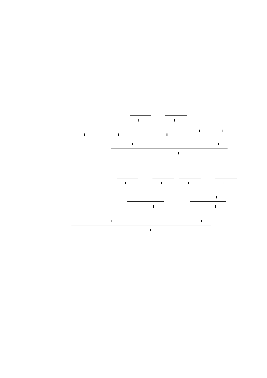
involving simpler formulae. In Classical Linear Logic we have the following
key-cases (excluding the additive key-cases which are similar to the corre-
sponding key-cases for Classical Logic):
15

Chapter 2.
Linear Logic
• The (⊗
R
,
⊗
L
) key-case
··
·
π
1
Γ
` A, ∆
··
·
π
2
Γ
0
` B, ∆
0
Γ, Γ
0
` A ⊗ B, ∆, ∆
0
··
·
π
0
1
Γ
00
, A, B
` ∆
00
Γ
00
, A
⊗ B ` ∆
00
Γ
00
, Γ, Γ
0
` ∆
00
, ∆, ∆
0
;
··
· π
1
Γ
` A, ∆
··
·
π
2
Γ
0
` B, ∆
0
··
·
π
0
1
Γ
00
, A, B
` ∆
00
Γ
00
, A, Γ
0
` ∆
00
, ∆
0
Γ
00
, Γ, Γ
0
` ∆
00
, ∆
0
, ∆
• The (I
R
, I
L
) key-case
` I
··
·
π
0
1
Γ
0
` ∆
0
Γ
0
, I
` ∆
0
Γ
0
` ∆
0
;
··
· π
0
1
Γ
0
` ∆
0
16

2.1.
Classical Linear Logic
• The ((
R
,
(
L
) key-case
··
·
π
1
Γ, A
` B, ∆
Γ
` A ( B, ∆
··
·
π
0
1
Γ
0
` A, ∆
0
··
·
π
0
2
Γ
00
, B
` ∆
00
Γ
0
, Γ
00
, A
( B ` ∆
00
, ∆
0
Γ
0
, Γ
00
, Γ
` ∆
00
, ∆
0
, ∆
;
··
· π
0
1
Γ
0
` A, ∆
0
··
· π
1
Γ, A
` B, ∆
··
·
π
0
2
Γ
00
, B
` ∆
00
Γ
00
, Γ, A
` ∆
00
, ∆
Γ
00
, Γ, Γ
0
` ∆
00
, ∆, ∆
0
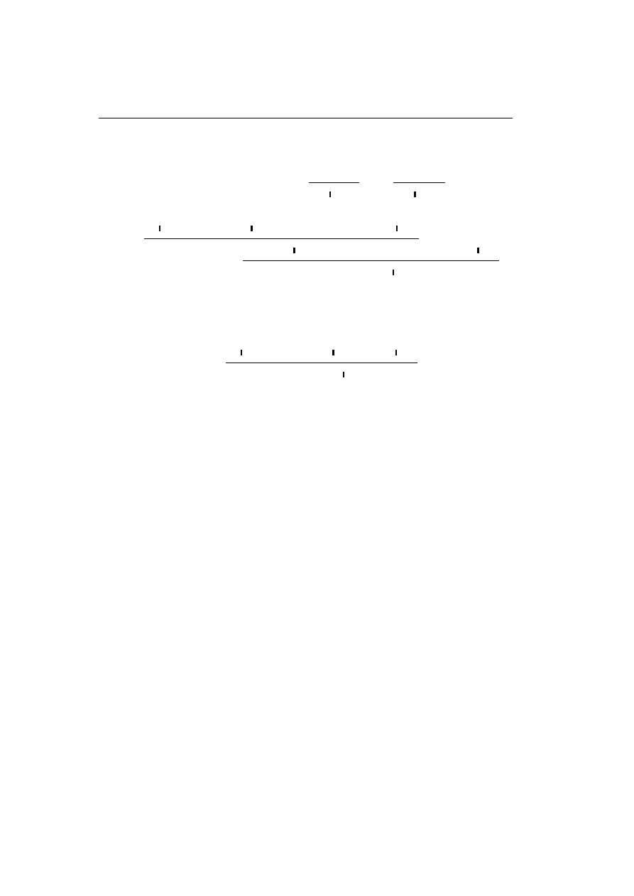
• The (!
R
, !
L
) key-case
··
· π
1
!Γ
` A, ?∆
!Γ
`!A, ?∆
··
· π
0
1
Γ
0
, A
` ∆
0
Γ
0
, !A
` ∆
0
Γ
0
, !Γ
` ∆
0
, ?∆
;
··
· π
1
!Γ
` A, ?∆
··
· π
0
1
Γ
0
, A
` ∆
0
Γ
0
, !Γ
` ∆
0
, ?∆
• The (!
R
, W
L
) key-case
··
· π
1
!Γ
` A, ?∆
!Γ
`!A, ?∆
··
· π
0
1
Γ
0
` ∆
0
Γ
0
, !A
` ∆
0
Γ
0
, !Γ
` ∆
0
, ?∆
;
··
· π
0
1
Γ
0
` ∆
0
===========
Γ
0
, !Γ
` ∆
0
, ?∆
We also have (
.............................
......
..
............
...........
....
..
..
...
....
...........
.........
R
,
.............................
......
..
............
...........
....
..
..
...
....
...........
.........
L
), (
⊥
R
,
⊥
L
), (W
R
, ?
L
), and (?
R
, ?
L
) key-cases, but they
are left out as they are symmetric to the mentioned (
⊗
R
,
⊗
L
), (I
R
, I
L
),
17

Chapter 2.
Linear Logic
(!
R
, W
L
), and (!
R
, !
L
) cases, respectively. The key-cases have the property
that a cut is replaced by cuts involving simpler formulas. Furthermore we
have the following so-called pseudo key-case:
• The (!
R
, C
L
) pseudo key-case
··
·
π
1
!Γ
` A, ?∆
!Γ
`!A, ?∆
··
·
π
0
1
Γ
0
, !A, !A
` ∆
0
Γ
0
, !A
` ∆
0
Γ
0
, !Γ
` ∆
0
, ?∆
;
··
· π
1
!Γ
` A, ?∆
!Γ
`!A, ?∆
··
· π
1
!Γ
` A, ?∆
!Γ
`!A, ?∆
··
· π
0
1
Γ
0
, !A, !A
` ∆
0
Γ
0
, !Γ, !A
` ∆
0
, ?∆
Γ
0
, !Γ, !Γ
` ∆
0
, ?∆, ?∆
=================
Γ
0
, !Γ
` ∆
0
, ?∆
We also have a (C
R
, ?
L
) pseudo key-case, but this is left out as it is symmetric
to the mentioned (!
R
, C
L
) case.
Note that in a pseudo key-case the cut
formula is replaced by cuts involving the same formula. Hence, the pseudo
key-cases does not simplify the involved cut formulas, which distinguishes
them from the key-cases (and this is indeed the reason why we call them
pseudo key-cases). In Appendix B we shall give a proof of cut-elimination
for the multiplicative fragment. As with Classical Logic, it is the case that
Classical Linear Logic satisfies the subformula property, that is, all formulae
occuring in a cut-free proof are subformulae of the formulae occuring in the
end-sequent.
Classical Linear Logic does not satisfy Church-Rosser, but on the other
hand, it is possible to give a non-trivial sound denotational semantics using
coherence spaces, see [GLT89]. Thus, the non-determinism of cut-elimination
18

2.2.
Intuitionistic Linear Logic
for Classical Linear Logic is limited. Note also that the example of Section 1.1
showing the non-determinism of cut-elimination for Classical Logic does not
go through for Classical Linear Logic.
It is, however, the case that the
multiplicative fragment of Classical Linear Logic satisfies Church-Rosser, cf.
[Laf96]. A proof can be found in [Dan90].
2.2
Intuitionistic Linear Logic
This section deals with Intuitionistic Linear Logic. The formulae are the same
as with Classical Linear Logic except that those involving the connectives
⊥,
.............................
......
..
............
...........
....
..
..
...
....
..........
..
........
and ? are omitted. The proof-rules of Intuitionistic Linear Logic in
Gentzen style occur as those of Classical Linear Logic given in Appendix A.3
where the proof-rules are subject to the restriction that each right hand side
context contains exactly one formula. It is possible to deal with the
⊥,
.............................
......
..
...........
...........
.....
..
..
..
....
...........
..
........
and ? connectives intuitionistically by allowing sequents to have more than
one conclusion together with an appropriate restriction on the
(
R
rule -
see [BdP96, HdP93]. It turns out that the ! modality enables Intuitionistic
Logic to be interpreted faithfully in Intuitionistic Linear Logic via the Girard
Translation - see Section 2.6.
Here we shall also consider a Natural Deduction presentation of Intu-
itionistic Linear Logic which is equivalent to the Gentzen style formulation.
Proof-rules for this formulation of the logic are given in Appendix A.4; they
are used to derive sequents
A
1
, ..., A
n
− B.
The Natural Deduction presentation is the same as the one given in the paper
[BBdPH92], and later fleshed out in detail in [Bie94]. A historical account
of the Natural Deduction presentation of Intuitionistic Linear Logic can be
found in Section 4.4 of [Bra96].
As in Intuitionistic Logic, a proof might be rewritten into a simpler form
using a reduction rule. Again, reduction of a Natural Deduction proof cor-
responds to cut-eliminating in a Gentzen style formulation. The reduction
rules of the Natural Deduction presentation of Intuitionistic Linear Logic
given here are as follows (excluding the additive reductions which are similar
to the corresponding reductions for Intuitionistic Logic):
19
Chapter 2.
Linear Logic
• The (I
I
, I
E
) case
− I
··
·
Γ
− A
Γ
− A
;
··
·
Γ
− A
• The (⊗
I
,
⊗
E
) case
··
·
Γ
− A
··
·
∆
− B
Γ, ∆
− A ⊗ B
A
− A B − B
··
·
Λ, A, B
− C
Λ, Γ, ∆
− C
;
··
·
Γ
− A
··
·
∆
− B
··
·
Λ, Γ, ∆
− C
• The ((
I
,
(
E
) case
A
− A
··
·
Γ, A
− B
Γ
− A ( B
··
·
Λ
− A
Γ, Λ
− B
;
··
·
Λ
− A
··
·
Γ, Λ
− B
20
2.2.
Intuitionistic Linear Logic
• The (P romotion, Dereliction) case
··
·
Γ
1
− !A
1
, ... ,
··
·
Γ
n
− !A
n
!A
1
− !A
1
, ..., !A
n
− !A
n
··
·
!A
1
, ..., !A
n
− B
Γ
1
, ..., Γ
n
− !B
Γ
1
, ..., Γ
n
− B
;
··
·
Γ
1
− !A
1
, ...,
··
·
Γ
n
− !A
n
··
·
Γ
1
, ..., Γ
n
− B
21
Chapter 2.
Linear Logic
• The (P romotion, Contraction) case
··
·
Γ
1
− !A
1
, ...,
··
·
Γ
n
− !A
n
!A
1
− !A
1
, ..., !A
n
− !A
n
··
·
!A
1
, ..., !A
n
− B
Γ
1
, ..., Γ
n
− !B
!B
− !B !B − !B
··
·
Λ, !B, !B
− C
Λ, Γ
1
, ..., Γ
n
− C
;
··
·
Γ
1
− !A
1
, ...,
··
·
Γ
n
− !A
n
!A
1
− !A
1
, ..., !A
n
− !A
n
··
·
!A
1
, ..., !A
n
− B
!A
1
, ..., !A
n
− !B
!A
1
− !A
1
, ..., !A
n
− !A
n
··
·
!A
1
, ..., !A
n
− B
!A
1
, ..., !A
n
− !B
··
·
Λ, !A
1
, ..., !A
n
, !A
1
, ..., !A
n
− C
Λ, Γ
1
, ..., Γ
n
− C
where the last used rule is derivable by using the Contraction and
Exchange rules. Note that a special case of the Contraction rule is
used.
22
2.3.
A Digression - Russell’s Paradox and Linear Logic
• The (P romotion, W eakening) case
··
·
Γ
1
− !A
1
, ... ,
··
·
Γ
n
− !A
n
!A
1
− !A
1
, ..., !A
n
− !A
n
··
·
!A
1
, ..., !A
n
− B
Γ
1
, ..., Γ
n
− !B
Λ
− C
Λ, Γ
1
, ..., Γ
n
− C
;
··
·
Γ
1
− !A
1
, ... ,
··
·
Γ
n
− !A
n
Λ
− C
Λ, Γ
1
, ..., Γ
n
− C
where the last used rule is derivable by using the W eakening rule.
If we think of the P romotion rule as putting a “box” around the right
hand side proof, then (P romotion, Dereliction) reduction removes the box,
whereas the (P romotion, Contraction) and (P romotion, W eakening) reduc-
tions respectively copy and discard the box.
Notions of Church-Rosser and strong normalisation for the Natural De-
duction presentation of Intuitionistic Linear Logic are defined in analogy
with the notions of Church-Rosser and strong normalisation for Intuitionis-
tic Logic. Intuitionistic Linear Logic does indeed satisfy these properties; via
a Curry-Howard isomorphism this corresponds to analogous results for reduc-
tion of terms of the linear λ-calculus which we will return to in Section 2.4
and Section 2.5.
2.3
A Digression - Russell’s Paradox and
Linear Logic
In this section we will make a digression with the aim of illustrating the fine
grained character of Intuitionistic Linear Logic compared to Intuitionistic
23

Chapter 2.
Linear Logic
Logic. We will take set-theoretic comprehension into account: In both of the
logics unrestricted comprehension enables a contradiction to be proved via
Russell’s Paradox, but it turns out that Intuitionistic Linear Logic allows the
presence of a restricted form of comprehension, which is not possible in the
case of Intuitionistic Logic.
Unrestricted comprehension says that for any predicate A(x) there is a
set
{x | A(x)} with the property that
t
∈ {x | A(x)} ⇔ A(t).
This is a very strong axiom; it has all the axioms of Zermelo-Fraenkel set
theory except the Axiom of Choice as special cases. An informal proof of
Russell’s Paradox now goes as follows: Using comprehension we define a set
u as
u =
{x | ¬(x ∈ x)}.
Thus, u is the famous set of all those sets that are not elements of themselves.
We then define a formula R to be
u
∈ u.
We then have R
⇔ ¬R which enables a contradiction to be proved as follows:
Assume R, this entails
¬R, which together with R entails a contradiction.
Thus we have proved
¬R. The proof of ¬R also gives a proof of R. But a
proof of
¬R together with a proof of R entails a contradiction.
Note how the contradiction is proved in two stages: First a formula R
such that R
⇔ ¬R is defined, then a contradiction is derived in a proof where
the assumption R is used twice. The two applications of the assumption R
are emphasised in the informal proof above. The are two ways of remedying
this inconsistency:
• Unrestricted comprehension is replaced by weaker axioms such that it
is impossible to define the set u and hence the formula R with the
property that R
⇔ ¬R cannot be defined either. This was the option
taken historically and which gave rise to Zermelo-Fraenkel set theory.
• Unrestricted comprehension is kept but the surrounding logic is weak-
ened such that the existence of a formula R with the property that
R
⇔ ¬R does not imply a contradiction. The !-free fragment of Linear
24

2.3.
A Digression - Russell’s Paradox and Linear Logic
Logic is one such option as assumptions here can be used only once
(recall that in deriving a contradiction from R
⇔ ¬R the assumption
R is used twice).
We will now flesh out some details of the second option. First we give a formal
proof of Russell’s Paradox in Intuitionistic Logic extended with unrestricted
comprehension as prescribed in [Pra65]. Recall that in Intuitionistic Logic
negation
¬A is defined as A ⇒ 0. The grammar for formulae of Intuitionistic
Logic is extended with an additional clause
s ::= ...
| t ∈ t
and a grammar for terms is added
t ::= x
| {x | s}
where x is a variable ranging over terms. Terms are to be thought of as sets
(they should not be confused with terms of the λ-calculus). Furthermore,
proof-rules for introduction and elimination of the connective
∈ are added
Γ
` A[t/x]
∈
I
Γ
` t ∈ {x | A}
Γ
` t ∈ {x | A}
∈
E
Γ
` A[t/x]
The first stage of Russell’s Paradox is formalised as follows: We define the
term u and the formula R as above and get
Γ
` R
Γ
` ¬R
and vice versa, which is equivalent to provability of
` R ⇒ ¬R and vice
versa. The second stage of the paradox is formalised as follows: Two copies
of the proof
R
` R
R
` ¬R
R
` R
R, R
` 0
R
` 0
` ¬R
25

Chapter 2.
Linear Logic
are applied in the proof
··
·
` ¬R
` R
··
·
` ¬R
` 0
of a contradiction. Note that we have used the admissible contraction proof-
rule together with a multiplicative version of the
⇒
E
rule which is also ad-
missible in Intuitionistic Logic. The presence of contraction is crucial for the
proof of inconsistency to go through. In [Pra65] the following observation
is made: It can be shown that the sequent
` 0 is not provable by a normal
proof; this means that no reduction sequences originating from the proof of
` 0 above end in a normal proof. Indeed, the proof reduces in two stages to
itself by carrying out the only performable reductions.
Now, above we have shown that unrestricted comprehension in the con-
text of Intuitionistic Logic is inconsistent. But it turns out that we do not get
inconsistency if we extend the !-free fragment of Intuitionistic Linear Logic
with unrestricted comprehension as above. Negation
¬A is here defined as
A
( 0
1
. We still have a formula R such that R
( ¬R and vice versa, but
now we cannot prove
− 0 as before because contraction is forbidden. The
system was proved consistent in [Gri82] using the following two observations:
A proof essentially shrinks under normalisation and there is no normal proof
of
− 0. The !-free fragment of Intuitionistic Linear Logic with unrestricted
comprehension is, however, very unexpressive. A partial solution to this lack
of expressiveness is to extend Intuitionistic Linear Logic with comprehension
as above but with the restriction that the ! modality is not allowed to occur in
the involved formula A(t). We still have the formula R such that R
( ¬R
and vice versa, but it turns out that this system is consistent, which was
proved in [Shi94].
Hence, the fine-grainedness of Intuitionistic Linear Logic allows the pres-
ence of a restricted form of comprehension, which is not possible in the
context of Intuitionistic Logic. It should be mentioned that considerations
on Russell’s Paradox in the context of Linear Logic have been crucial for
Girard’s discovery of Light Linear Logic - see [Gir94].
1
This is not the same as the negation A
⊥
of Classical Linear Logic which is defined as
A
⊥
= A
(
⊥. However, this difference is not of importance here.
26

2.4.
The Linear
λ-Calculus
2.4
The Linear λ-Calculus
The presentation of the linear λ-calculus which we give in this section is
the same as the one given in [BBdPH92, BBdPH93], and later fleshed out in
detail in [Bie94]. We have omitted the additive fragment as it is similar to the
corresponding fragment of the λ-calculus. The next section shows how the
linear λ-calculus occurs as a Curry-Howard interpretation of Intuitionistic
Linear Logic in the same way as the λ-calculus occurs as a Curry-Howard
interpretation of Intuitionistic Logic. Types of the linear λ-calculus are given
by the grammar
s ::= I
| s ⊗ s | s ( s | !s
and terms are given by the grammar
t ::=
x
|
∗ | let t be ∗ in t | t ⊗ t | let t be x ⊗ y in t |
λx
A
.t
| tt |
promote t, ..., t for x
1
, ..., x
n
in t
| derelict(t) |
discard t in t
| copy t as x, y in t
where x is a variable ranging over terms and t, ..., t denotes a list of n occur-
rences of the symbol t. The set of free variables, denoted F V (u), of a term
u is defined by induction on u as follows:
F V (x) =
{x}
F V (
∗) = ∅
F V (let w be
∗ in u) = F V (w) ∪ F V (u)
F V (u
⊗ v) = F V (u) ∪ F V (v)
F V (let w be x
⊗ y in u) = F V (w) ∪ F V (u) − {x, y}
F V (λx.u) = F V (u)
− {x}
F V (f u) = F V (f )
∪ F V (u)
F V (promote v
1
, ..., v
n
for x
1
, ..., x
n
in u) = F V (v
1
)
∪ ... ∪ F V (v
n
)
F V (derelict(u)) = F V (u)
F V (discard w in u) = F V (w)
∪ F V (u)
F V (copy w as x, y in u) = F V (w)
∪ F V (u) − {x, y}
27
Chapter 2.
Linear Logic
Figure 2.1: Type Assignment Rules for the Linear λ-Calculus
x : A
− x : A
Γ, x : A, y : B, ∆
− u : C
Γ, y : B, x : A, ∆
− u : C
− ∗ : I
Λ
− w : I Γ − u : A
Γ, Λ
− let w be ∗ in u : A
Γ
− u : A ∆ − v : B
Γ, ∆
− u ⊗ v : A ⊗ B
Λ
− w : A ⊗ B Γ, x : A, y : B − u : C
Γ, Λ
− let w be x ⊗ y in u : C
Γ, x : A
− u : B
Γ
− λx
A
.u : A
( B
Λ
− f : A ( B ∆ − u : A
Λ, ∆
− fu : B
Γ
1
− v
1
:!A
1
, ... , Γ
n
− v
n
:!A
n
x
1
:!A
1
, ..., x
n
:!A
n
− u : B
Γ
1
, ..., Γ
n
− promote v
1
, ..., v
n
for x
1
, ..., x
n
in u :!B
Λ
− u :!B
Λ
− derelict(u) : B
Λ
− w :!A Γ, x :!A, y :!A − u : B
Γ, Λ
− copy w as x, y in u : B
Λ
− w :!A Γ − u : B
Γ, Λ
− discard w in u : B
28

2.4.
The Linear
λ-Calculus
We use the same convention concerning substitution as for terms of the λ-
calculus: If a term v together with n terms u
1
, ..., u
n
and n pairwise distinct
variables x
1
, ..., x
n
are given, then v[u
1
, ..., u
n
/x
1
, ..., x
n
] denotes the term
v where simultaneously the terms u
1
, ..., u
n
have been substituted for free
occurrences of the variables x
1
, ..., x
n
such that bound variables in v have
been renamed to avoid capture of free variables of the terms u
1
, ..., u
n
.
Rules for assignment of types to terms are given in Appendix A.4. Type
assignments have the form of sequents
x
1
: A
1
, ..., x
n
: A
n
− u : A
where x
1
, ..., x
n
are pairwise distinct variables. Note that the definition of
sequents implicitly restricts use of the rules. For example, it is not possible
to use the rule for introduction of
⊗ if the contexts Γ and ∆ have common
variables. By induction on the derivation of the type assignment it can be
shown that
F V (u) =
{x
1
, ..., x
n
}.
Note that this is different from the λ-calculus where we did not have equality,
but only an inclusion. By induction on the derivation of the type assignment
it can be shown that every free variable of the term u occurs exactly once
2
.
The linear λ-calculus satisfies the following properties:
Lemma 2.4.1 If the sequent Γ
− u : A is derivable, then for any derivable
sequent Γ
0
− u : B, where the context Γ
0
is a permutation of the context Γ,
we have A = B.
Proof: Induction on the derivation of Γ
− u : A.
2
The following proposition is the essence of the Curry-Howard isomorphism:
Proposition 2.4.2 If the sequent Γ
− u : A is derivable, then the first
rule instance above the sequent which is different from an instance of the
Exchange rule is uniquely determined up to permutation of the context Γ.
Proof: Use Lemma 2.4.1 to check each case.
2
Now comes a lemma dealing with substitution.
2
This does not hold if the additive fragment is included.
29

Chapter 2.
Linear Logic
Lemma 2.4.3 (Substitution Property) If both of the sequents Γ
− u : A and
∆, x : A, Λ
− v : B are derivable and the variables in the contexts Γ and ∆, Λ
are pairwise distinct, then the sequent ∆, Γ, Λ
− v[u/x] : B is also derivable.
Proof: Induction on the derivation of ∆, x : A, Λ
− v : B.
2
We now need a couple of conventions: The term
copy w
1
as x
1
, y
1
in (...copy w
n
as x
n
, y
n
in u...)
is denoted
copy w as x, y in u
and the term
discard w
1
in (...discard w
n
in u...)
is denoted
discard w in u.
The linear λ-calculus has the following β-reduction rules each of which is
the image under the Curry-Howard isomorphism of a reduction on the proof
corresponding to the involved term:
let
∗ be ∗ in u
;
u
u
⊗ v be x ⊗ y in w
;
w[u, v/x, y]
(λx.u)w
;
u[w/x]
derelict(promote w for x in u)
;
v[w/x]
discard (promote w for x in u) in v
;
discard w in v
copy (promote w for x in u) as y, z in v
;
copy w as x
0
, x
00
in (v[promote x
0
for x in u, promote x
00
for x in u/y, z])
30

2.5.
The Curry-Howard Isomorphism
We shall only be concerned with β-reductions. The properties of Church-
Rosser and strong normalisation for proofs of Intuitionistic Linear Logic cor-
respond to analogous notions for terms of the linear λ-calculus via the Curry-
Howard isomorphism. In [Ben93] it is shown that the linear λ-calculus sat-
isfies strong normalisation by giving a reduction preserving translation into
System F (which does satisfy strong normalisation). By K¨
onig’s Lemma, this
implies that all terms are bounded. Church-Rosser can then be proved in
the standard way by induction on the bound. The proof is straightforward,
but tedious.
2.5
The Curry-Howard Isomorphism
In what follows, we will consider the Natural Deduction presentation of In-
tuitionistic Linear Logic given in Appendix A.4. Intuitionistic Linear Logic
corresponds to the linear λ-calculus via a Curry-Howard isomorphism in the
same way as Intuitionistic Logic corresponds to the λ-calculus. The formulae
of Intuitionistic Linear Logic correspond to types of the linear λ-calculus in
the obvious way. We get the rules for assigning types to terms of the linear
λ-calculus if we decorate the proof-rules of Intuitionistic Linear Logic with
terms in the appropriate way, and moreover, we can recover the proof-rules if
we take the typing rules of the linear λ-calculus and remove the terms. The
isomorphism on the level of proofs is essentially given by Proposition 2.4.2.
As with the λ-calculus, it is the case that all the β-reductions of the
linear λ-calculus appear as Curry-Howard interpretations of reduction rules of
Intuitionistic Linear Logic. For example, in the case of a (
⊗
I
,
⊗
E
) reduction
31
Chapter 2.
Linear Logic
we get
··
·
Γ
− u : A
··
·
∆
− v : B
Γ, ∆
− u ⊗ v : A ⊗ B
x : A
− x : A y : B − y : B
··
·
Λ, x : A, y : B
− wC
Λ, Γ, ∆
− let u ⊗ v be x ⊗ y in w : C
;
··
·
Γ
− u : A
··
·
∆
− v : B
··
·
Λ, Γ, ∆
− w[u, v/x, y] : C
We see that a β-reduction has taken place on the term encoding the proof
on which the reduction is performed. All β-reductions actually do appear as
Curry-Howard interpretations of reductions on the corresponding proofs.
2.6
The Girard Translation
The [Gir87] paper introduced the Girard Translation which embeds Intuition-
istic Logic into Intuitionistic Linear Logic. We will state the Girard Transla-
tion in terms of the Natural Deduction presentations of Intuitionistic Logic
and Intuitionistic Linear Logic given in Appendix A.2 and Appendix A.4,
respectively. The translation works at the level of formulae as well as at the
level of proofs. At the level of formulae the Girard Translation is defined
inductively as follows:
1
o
= 1
(A
∧ B)
o
= A
o
&B
o
(A
⇒ B)
o
= !A
o
( B
o
0
o
= 0
(A
∨ B)
o
= !A
o
⊕!B
o
32
2.6.
The Girard Translation
At the level of proofs the Girard Translation inductively translates a proof
of a sequent
A
1
, ..., A
n
` B
into a proof of the sequent
!A
o
1
, ..., !A
o
n
− B
o
.
In what follows we consider each case except the symmetric ones. Special
cases of rules are used when appropriate. Recall that a double bar means a
number of applications of rules.
• A derivation
A
1
, ..., A
n
` A
p
is translated into
!A
o
q
− !A
o
p
!A
o
q
− A
o
p
=============
!A
o
1
, ..., !A
o
n
− A
o
p
• A derivation
Γ
` 1
is translated into
!Γ
o
− 1
• A derivation
Γ
` A Γ ` B
Γ
` A ∧ B
is translated into
!Γ
o
− A
o
!Γ
o
− B
o
!Γ
o
− A
o
&B
o
• A derivation
Γ
` A ∧ B
Γ
` A
is translated into
!Γ
o
− A
o
&B
o
!Γ
o
− A
o
33
Chapter 2.
Linear Logic
• A derivation
Γ, A
` B
Γ
` A ⇒ B
is translated into
!Γ
o
, !A
o
− B
o
!Γ
o
− !A
o
( B
o
• A derivation
Γ
` A ⇒ B Γ ` A
Γ
` B
is translated into
!Γ
o
− !A
o
( B
o
!Γ
o
− A
o
!Γ
o
− !A
o
!Γ
o
, !Γ
o
− B
o
==========
!Γ
o
− B
o
• A derivation
Γ
` 0
Γ
` C
is translated into
!Γ
o
− 0
!Γ
o
− C
o
• A derivation
Γ
` A
Γ
` A ∨ B
is translated into
!Γ
o
− A
o
!Γ
o
− !A
o
!Γ
o
− !A
o
⊕!B
o
• A derivation
Γ
` A ∨ B Γ, A ` C Γ, B ` C
Γ
` C
34
2.7.
Concrete Models
is translated into
!Γ
o
− !A
o
⊕!B
o
!Γ
o
, !A
o
− C
o
!Γ
o
, !B
o
− C
o
!Γ
o
, !Γ
o
− C
o
==========
!Γ
o
− C
o
The translation is sound with respect to provability in the sense that the
sequent A
1
, ..., A
n
` B is provable (in Intuitionistic Logic) iff !A
o
1
, ..., !A
o
n
− B
o
is provable (in Intuitionistic Linear Logic). Moreover, it is shown in [Bie94]
that the translation preserves β-reductions. In [Gir87] it is shown that the
Girard Translation is sound with respect to the standard coherence space
interpretation, that is, the interpretation of a proof in Intuitionistic Logic
is essentially the same as the interpretation of its image under the Girard
Translation. A categorical version of this result can be found in [Bra96].
2.7
Concrete Models
An example of a concrete model of Intuitionistic Linear Logic is the category
of cpos and strict continuous functions. A cpo is a partial order with the
property that each directed subset has a least upper bound. Note that this
entails that a cpo has a bottom element. A monotone function between cpos
is continuous if it preserves the least upper bound of any non-empty directed
subset, and it is strict if it preserves the bottom element. The symmetric
monoidal structure is given by the smash product, the internal-hom of two
objects is given by the set of strict continuous functions with the pointwise
order, and the comonad is given by the lift operation.
It should be mentioned that the category of cpos and strict continuous
functions is actually a model for intuitionistic relevant logic in the sense of
[Jac94].
Also the category of dI domains and linear stable functions is a model
of Intuitionistic Linear Logic. We will first define a dI domain. Let (D,
v)
be a non-empty poset such that every finitely bounded subset X has a least
upper bound
tX where a subset X is finitely bounded iff every finite subset
of X has an upper bound. This entails that D has a bottom element, and
moreover, every non-empty subset X has a greatest lower bound which we
will denote by
uX. A prime element of D is an element d such that
d
v tX ⇒ ∃x ∈ X. d v x
35

Chapter 2.
Linear Logic
for any finitely bounded subset X. We will denote the set of prime elements
of D by D
p
. The poset D is prime algebraic iff
∀d ∈ D. d = t{d
0
∈ D
p
| d
0
v d)}
A finite element of D is an element d such that
d
v tX ⇒ ∃x ∈ X. d v x
for any non-empty directed subset X. We will denote the set of finite elements
of D by D
o
. The poset D is finitary iff
∀d ∈ D
o
.
|{d
0
∈ D | d
0
v d}| < ∞
The poset D is a dI domain if it is prime algebraic and finitary. A mono-
tone function f between dI domains is stable iff f (
uX) = u{f(x) | x ∈ X}
for any non-empty finitely bounded subset X, and it is linear iff f (
tX) =
t{f(x) | x ∈ X} for any finitely bounded subset X. The trace tr(f) of a
linear stable function f : D
→ E is a subset of D
p
× E
p
defined as
{(d, e) ∈ D
p
× E
p
| e v f(d) ∧ ∀d
0
v d. (e v f(d
0
)
⇒ d = d
0
)
}
In what follows, X
↑ means that the subset X has an upper bound. The
tensor product D
⊗ E of two dI domains D and E is defined as
{t ⊆ D
p
× E
p
| π
1
(t)
↑ ∧π
2
(t)
↑ ∧t is down-closed }
ordered by inclusion. The unit I is defined to be the dI domain with two
elements. We define the internal-hom D
( E as
{tr(f) | f : D → E}
ordered by inclusion. This is called the stable order. The dI domain !D is
defined as
{t ⊆ D
o
| t ↑ ∧t is down-closed }
ordered by inclusion.
There are quite a few other concrete models of Intuitionistic Linear Logic
around. The traditional coherence space model should be mentioned - see
[Gir87] and [GLT89] for details. In another vein, there are the bistructure
model of [PW94] and the category of hypercoherences and strongly stable
linear functions of [Ehr93]. Recently, the game models of [AJM96, HO96,
Nic94] have gained attention as they give rise to fully abstract models of
Scott’s PCF.
36

Bibliography
[Abr90]
S. Abramsky.
Computational interpretations of linear logic.
Technical Report 90/20, Department of Computing, Imperial
College, 1990.
[AJM96]
S. Abramsky, R. Jagadeesan, and P. Malacaria. Full abstraction
for PCF. Submitted for publication, 1996.
[BBdPH92] N. Benton, G. Bierman, V. de Paiva, and M. Hyland. Term
assignment for intuitionistic linear logic. Technical Report 262,
Computer Laboratory, University of Cambridge, 1992.
[BBdPH93] N. Benton, G. Bierman, V. de Paiva, and M. Hyland. A term cal-
culus for intuitionistic linear logic. In Proceedings of TLCA ’93,
LNCS, volume 664. Springer-Verlag, 1993.
[BdP96]
T. Bra¨
uner and V. de Paiva. Cut-elimination for full intuition-
istic linear logic. Technical Report 395, Computer Laboratory,
University of Cambridge, 1996. 27 pages. Also available as Tech-
nical Report RS-96-10, BRICS, Department of Computer Sci-
ence, University of Aarhus.
[Ben93]
N. Benton. Strong normalisation for the linear term calculus.
Technical Report 305, Computer Laboratory, University of Cam-
bridge, 1993.
[Bie94]
G. Bierman. On Intuitionistic Linear Logic. PhD thesis, Com-
puter Laboratory, University of Cambridge, 1994.
37

BIBLIOGRAPHY
[Bra96]
T. Bra¨
uner. An Axiomatic Approach to Adequacy. PhD thesis,
Department of Computer Science, University of Aarhus, 1996.
168 pages.
[Dan90]
V. Danos. La Logique Lin´
eaire appliqu´
ee `
a l’´
etude de divers
processus de normalisation (principalement du λ-calcul). PhD
thesis, Universit´
e Paris VII, 1990.
[Ehr93]
T. Ehrhard. Hypercoherences: A strongly stable model of linear
logic. Mathematical Structures in Computer Science, 3, 1993.
[Gen34]
G. Gentzen. Untersuchungen ¨
uber das logische Schliessen. Math-
ematische Zeitschrift, 39, 1934.
[Gir87]
J.-Y. Girard. Linear logic. Theoretical Computer Science, 50,
1987.
[Gir89]
J.-Y. Girard. Towards a geometry of interaction. In Contempo-
rary Mathematics, Categories in Computer Science and Logic,
volume 92. American Mathematical Society, 1989.
[Gir91]
J.-Y. Girard. A new constructive logic: Classical logic. Mathe-
matical Structures in Computer Science, 1, 1991.
[Gir94]
J.-Y. Girard. Light linear logic. Manuscript, 1994.
[GLT89]
J.-Y. Girard, Y. Lafont, and P. Taylor. Proofs and Types. Cam-
bridge University Press, 1989.
[Gri82]
V. N. Grishin. Predicate and set-theoretic calculi based on logics
without contractions. Math. USSR Izvestiya, 18, 1982.
[HdP93]
M. Hyland and V. de Paiva. Full intuitionistic linear logic (ex-
tended abstract). Annals of Pure and Applied Logic, 64, 1993.
[HO96]
J. M. E. Hyland and C.-H. L. Ong. On full abstraction for PCF.
Submitted for publication, 1996.
[How80]
W. A. Howard. The formulae-as-type notion of construction. In
To H. B. Curry: Essays on Combinatory Logic, Lambda Calcu-
lus and Formalism. Academic Press, 1980.
38

BIBLIOGRAPHY
[Jac94]
B. Jacobs. Semantics of weakening and contraction. Annals of
Pure and Applied Logic, 69, 1994.
[Laf96]
Y. Lafont. Private communication, 1996.
[LS86]
J. Lambek and P. J. Scott. Introduction to higher order categor-
ical logic. Cambridge University Press, 1986.
[Nic94]
H. Nickau. Hereditarily sequential functionals. In Proceedings
of LFCS ’94, LNCS, volume 813. Springer-Verlag, 1994.
[Ong96]
C.-H. L. Ong.
A semantic view of classical proofs: Type-
theoretical, categorical, and denotational characterizations. In
11th LICS Conference. IEEE, 1996.
[Par91]
M. Parigot. Free deduction: An analysis of ”computations” in
classical logic.
In Proceedings of RCLP, LNCS, volume 592.
Springer-Verlag, 1991.
[Par92]
M. Parigot. λµ-calculus: An algorithmic interpretation of clas-
sical natural deduction. In Proceedings of LPAR, LNCS, volume
624. Springer-Verlag, 1992.
[Pra65]
D. Pravitz.
Natural Deduction. A Proof-Theoretical Study.
Almqvist and Wiksell, 1965.
[PW94]
G. Plotkin and G. Winskel. Bistructures, bidomains and lin-
ear logic. In Proceedings of ICALP ’94, LNCS, volume 820.
Springer-Verlag, 1994.
[Shi94]
M. Shirahata. Linear Set Theory. PhD thesis, Stanford Univer-
sity, 1994.
39

Appendix A
Logics
A.1
Classical Logic
Axiom
A
` A
Γ
` A, ∆ Γ
0
, A
` ∆
0
Cut
Γ
0
, Γ
` ∆
0
, ∆
Γ
` ∆
W eakening
L
Γ, A
` ∆
Γ
` ∆
W eakening
R
Γ
` A, ∆
Γ, A, A
` ∆
Contraction
L
Γ, A
` ∆
Γ
` A, A, ∆
Contraction
R
Γ
` A, ∆
Γ, A
` ∆
∧
L1
Γ, A
∧ B ` ∆
Γ, B
` ∆
∧
L2
Γ, A
∧ B ` ∆
Γ
` A, ∆ Γ
0
` B, ∆
0
∧
R
Γ, Γ
0
` A ∧ B, ∆, ∆
0
Γ
` ∆
1
L
Γ, 1
` ∆
1
R
` 1
Γ
` A, ∆ Γ
0
, B
` ∆
0
⇒
L
Γ, Γ
0
, A
⇒ B ` ∆, ∆
0
Γ, A
` B, ∆
⇒
R
Γ
` A ⇒ B, ∆
40

A.1.
Classical Logic
Classical Logic - Disjunction
Γ, A
` ∆ Γ
0
, B
` ∆
0
∨
L
Γ, Γ
0
, A
∨ B ` ∆, ∆
0
Γ
` A, ∆
∨
R1
Γ
` A ∨ B, ∆
Γ
` B, ∆
∨
R2
Γ
` A ∨ B, ∆
0
L
0
`
Γ
` ∆
0
R
Γ
` 0, ∆
41

Appendix A.
Logics
A.2
Intuitionistic Logic
Axiom
A
1
, ..., A
n
` A
q
1
I
Γ
` 1
Γ
` A Γ ` B
∧
I
Γ
` A ∧ B
Γ
` A ∧ B
∧
E1
Γ
` A
Γ
` A ∧ B
∧
E2
Γ
` B
Γ, A
` B
⇒
I
Γ
` A ⇒ B
Γ
` A ⇒ B Γ ` A
⇒
E
Γ
` B
Γ
` 0
0
E
Γ
` C
Γ
` A
∨
I1
Γ
` A ∨ B
Γ
` B
∨
I2
Γ
` A ∨ B
Γ
` A ∨ B Γ, A ` C Γ, B ` C
∨
E
Γ
` C
42
A.3.
Classical Linear Logic
A.3
Classical Linear Logic
Axiom
A
− A
Γ
− A, ∆ Γ
0
, A
− ∆
0
Cut
Γ
0
, Γ
− ∆
0
, ∆
Γ, A, B
− ∆
⊗
L
Γ, A
⊗ B − ∆
Γ
− A, ∆ Γ
0
− B, ∆
0
⊗
R
Γ, Γ
0
− A ⊗ B, ∆, ∆
0
Γ
− ∆
I
L
Γ, I
− ∆
I
R
− I
Γ, A
− ∆ Γ
0
, B
− ∆
0
.............................
......
..
...........
...........
....
...
..
..
....
...........
..
........
L
Γ, Γ
0
, A
.............................
......
..
...........
...........
....
...
..
..
....
...........
..
........
B
− ∆, ∆
0
Γ
− A, B, ∆
.............................
......
..
...........
...........
.....
..
..
..
....
...........
..
........
R
Γ
− A
.............................
......
..
...........
...........
.....
..
..
..
....
...........
..
........
B, ∆
⊥
L
⊥ −
Γ
− ∆
⊥
R
Γ
− ⊥, ∆
Γ
− A, ∆ Γ
0
, B
− ∆
0
(
L
Γ, Γ
0
, A
( B − ∆, ∆
0
Γ, A
− B, ∆
(
R
Γ
− A ( B, ∆
Γ, A
− ∆
!
L
Γ, !A
− ∆
!Γ
− A, ?∆
!
R
!Γ
− !A, ?∆
!Γ, A
− ?∆
?
L
!Γ, ?A
− ?∆
Γ
− A, ∆
?
R
Γ
− ?A, ∆
Γ
− ∆
W eakening
L
Γ, !A
− ∆
Γ
− ∆
W eakening
R
Γ
− ?A, ∆
Γ, !A, !A
− ∆
Contraction
L
Γ, !A
− ∆
Γ
− ?A, ?A, ∆
Contraction
R
Γ
− ?A, ∆
43
Appendix A.
Logics
Classical Linear Logic - the Additives
Γ, A
− ∆
&
L1
Γ, A&B
− ∆
Γ, B
− ∆
&
L2
Γ, A&B
− ∆
Γ
− A, ∆ Γ − B, ∆
&
R
Γ
− A&B, ∆
1
R
Γ
− 1, ∆
Γ, A
− ∆ Γ, B − ∆
⊕
L
Γ, A
⊕ B − ∆
Γ
− A, ∆
⊕
R1
Γ
− A ⊕ B, ∆
Γ
− B, ∆
⊕
R2
Γ
− A ⊕ B, ∆
0
L
Γ, 0
− ∆
44
A.4.
Intuitionistic Linear Logic
A.4
Intuitionistic Linear Logic
Axiom
A
− A
I
I
− I
Λ
− I Γ − A
I
E
Γ, Λ
− A
Γ
− A ∆ − B
⊗
I
Γ, ∆
− A ⊗ B
Λ
− A ⊗ B Γ, A, B − C
⊗
E
Γ, Λ
− C
Γ, A
− B
(
I
Γ
− A ( B
Λ
− A ( B ∆ − A
(
E
Λ, ∆
− B
Γ
1
− !A
1
, ..., Γ
n
− !A
n
!A
1
, ..., !A
n
− B
P rom.
Γ
1
, ..., Γ
n
− !B
Λ
− !B
Dereliction
Λ
− B
Λ
− !A Γ, !A, !A − B
Contraction
Γ, Λ
− B
Λ
− !A Γ − B
W eakening
Γ, Λ
− B
Γ
1
− A
1
, ... , Γ
n
− A
n
1
I
Γ
1
, ..., Γ
n
− 1
Γ
− A Γ − B
&
I
Γ
− A&B
Λ
− A&B
&
E1
Λ
− A
Λ
− A&B
&
E2
Λ
− B
Γ
1
− A
1
, ... , Γ
n
− A
n
Λ
− 0
0
E
Γ
1
, ..., Γ
n
, Λ
− C
Γ
− A
⊕
I1
Γ
− A ⊕ B
Γ
− B
⊕
I2
Γ
− A ⊕ B
Λ
− A ⊕ B Γ, A − C Γ, B − C
⊕
E
Γ, Λ
− C
45

Appendix B
Cut-Elimination for Classical
Linear Logic
In this appendix we show that the multiplicative fragment of Classical Linear
Logic satisfies the cut-elimination property. We actually give an algorithm
transforming an arbitrary Classical Linear Logic proof (in the multiplicative
fragment) into a cut-free proof with the same end-sequent. Our proof of
cut-elimination is essentially taken from [BdP96]; it is along the lines of the
proof of cut-elimination for Classical Logic given in [GLT89] where the linear
context is taken into account. Towards the goal of proving this theorem we
start with some preliminary results.
B.1
Some Preliminary Results
As usual with cut-elimination proofs, a cut can either be replaced by cuts
involving simpler formulas, or it can be pushed upwards in the surrounding
proof. The former situation amounts to the key-cases, and the latter situation
is exemplified by the proof
Γ
− A, ∆
Γ
1
, A
− ∆
1
r
0
Γ
0
, A
− ∆
0
Γ
0
, Γ
− ∆
0
, ∆
which is transformed into
46
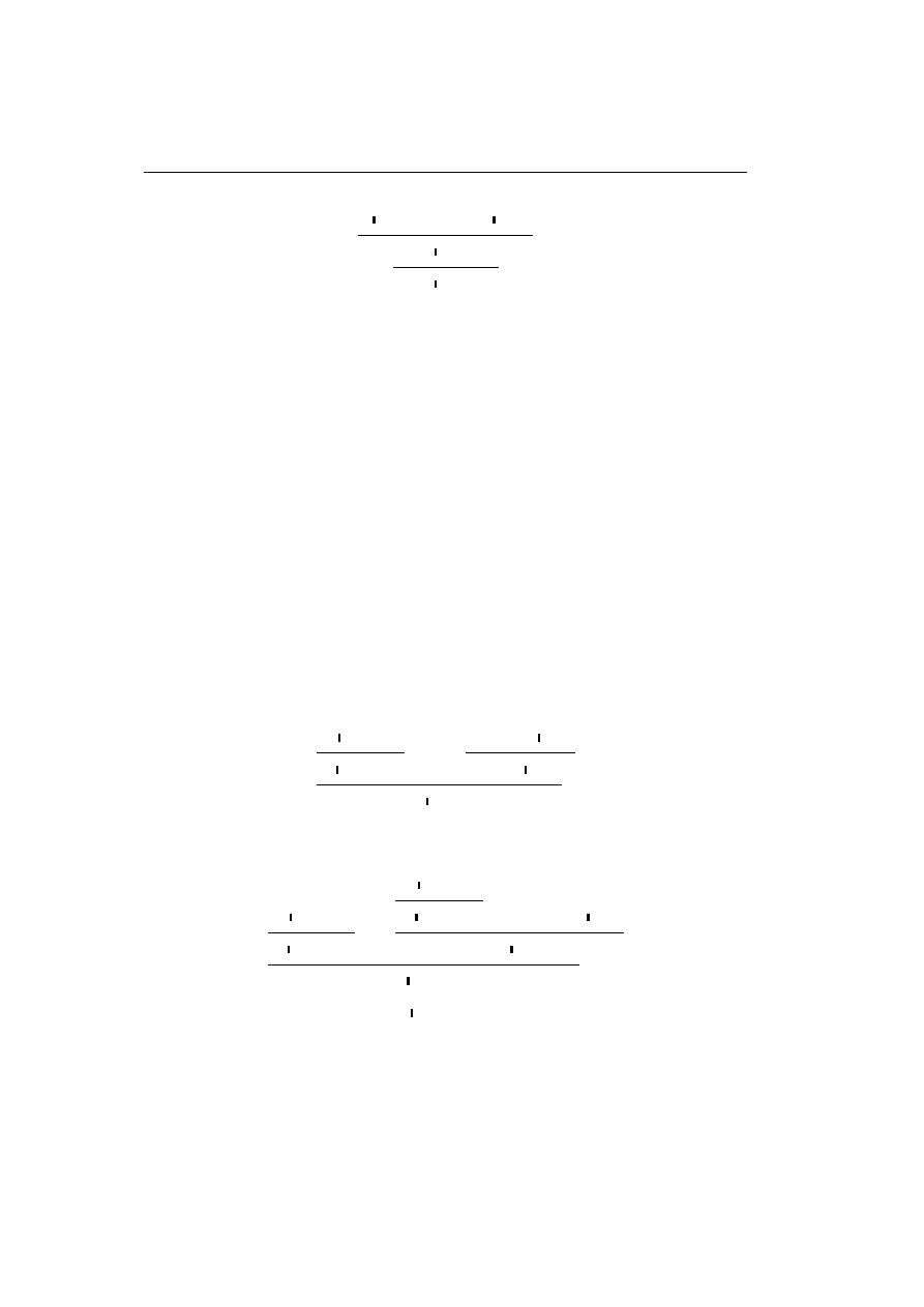
B.1.
Some Preliminary Results
Γ
− A, ∆ Γ
1
, A
− ∆
1
Γ
1
, Γ
− ∆
1
, ∆
r
0
Γ
0
, Γ
− ∆
0
, ∆
As is usual in cut-elimination proofs we need to define the degree of a formula.
Definition B.1.1 The degree ∂(A) of a formula A is defined inductively as
follows:
1. ∂(A) = 1 when A is atomic
2. ∂(A
⊗ B) = ∂(A
.............................
......
..
............
...........
....
...
..
...
.....
.........
.........
B) = ∂(A
( B) = max{∂(A), ∂(B)} + 1
3. ∂(!A) = ∂(?A) = ∂(A) + 1
The degree of a cut is defined to be the degree of the formula cut. The degree
of a proof is defined as the supremum of the degrees of the cuts in the proof.
The fundamental property of the key-cases is that a cut is replaced by cuts
of strictly lower degree.
Now we deal with what we call the pseudo key-cases, which differ from the
key-cases in that they do not decrease the degree of the cuts involved. There
are two pseudo key-cases, namely (!
R
, C
L
) and (C
R
, ?
L
). In Lemma B.1.3
we show how to perform additional modifications when applying the pseudo
key-cases such that the degree of the involved cuts does decrease. Let us
examine the (!
R
, C
L
) pseudo key-case
!Γ
− A, ?∆
!
R
!Γ
− !A, ?∆
Γ
0
, !A, !A
− ∆
0
Γ
0
, !A
− ∆
0
Γ
0
, !Γ
− ∆
0
, ?∆
;
!Γ
− A, ?∆
!Γ
− !A, ?∆
!Γ
− A, ?∆
!Γ
− !A, ?∆
Γ
0
, !A, !A
− ∆
0
Γ
0
, !Γ, !A
− ∆
0
, ?∆
Γ
0
, !Γ, !Γ
− ∆
0
, ?∆, ?∆
=================
Γ
0
, !Γ
− ∆
0
, ?∆
47
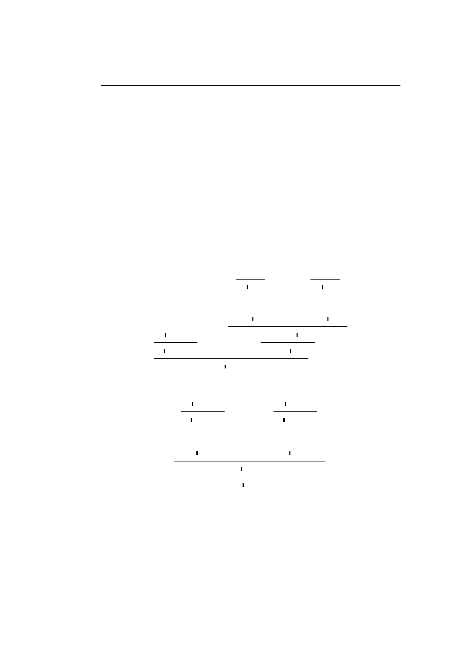
Appendix B.
Cut-Elimination for Classical Linear Logic
The (!
R
, C
L
) pseudo key-case does not decrease the degree, as mentioned
above. Thus, instead of just modifying the proof as prescribed, we have
to “track” the cut formula !A upwards in the right hand side immediate
subproof which has C
L
as the last rule. When we follow an antecedent !A
formula upwards in a proof, then a track ends due to one of the following
reasons: The formula is introduced by an instance of the !
L
rule, the formula
is absorbed by an instance of the W
L
rule, or finally, we end up in an axiom.
Note that on the way upwards the formula !A might have proliferated into
several copies while passing instances of the C
L
rule. In each of the mentioned
end-points there is an appropriate way of modifying the proof such that !A
is replaced by !Γ and ?∆ is added on the succedent in a way that decreases
the degree. For example the following proof where none of the tracks are
proliferated by passing instances of the C
L
rule and they both both end up
in an axiom
!Γ
− A, ?∆
!
R
!Γ
− !A, ?∆
!A
− !A
·
·
·
Γ
1
, !A
− ∆
1
!A
− !A
·
·
·
Γ
2
, !A
− ∆
2
Γ
0
, !A, !A
− ∆
0
Γ
0
, !A
− ∆
0
Γ
0
, !Γ
− ∆
0
, ?∆
is modified as follows
!Γ
− A, ?∆
!
R
!Γ
− !A, ?∆
·
·
·
Γ
1
, !Γ
− ∆
1
, ?∆
!Γ
− A, ?∆
!
R
!Γ
− !A, ?∆
·
·
·
Γ
2
, !Γ
− ∆
2
, ?∆
Γ
0
, !Γ, !Γ
− ∆
0
, ?∆, ?∆
=================
Γ
0
, !Γ
− ∆
0
, ?∆
Note that a (!
R
, C
L
) pseudo key-case was performed in the process of following
the track(s) upwards. This is formalised in the next lemma which takes care
48
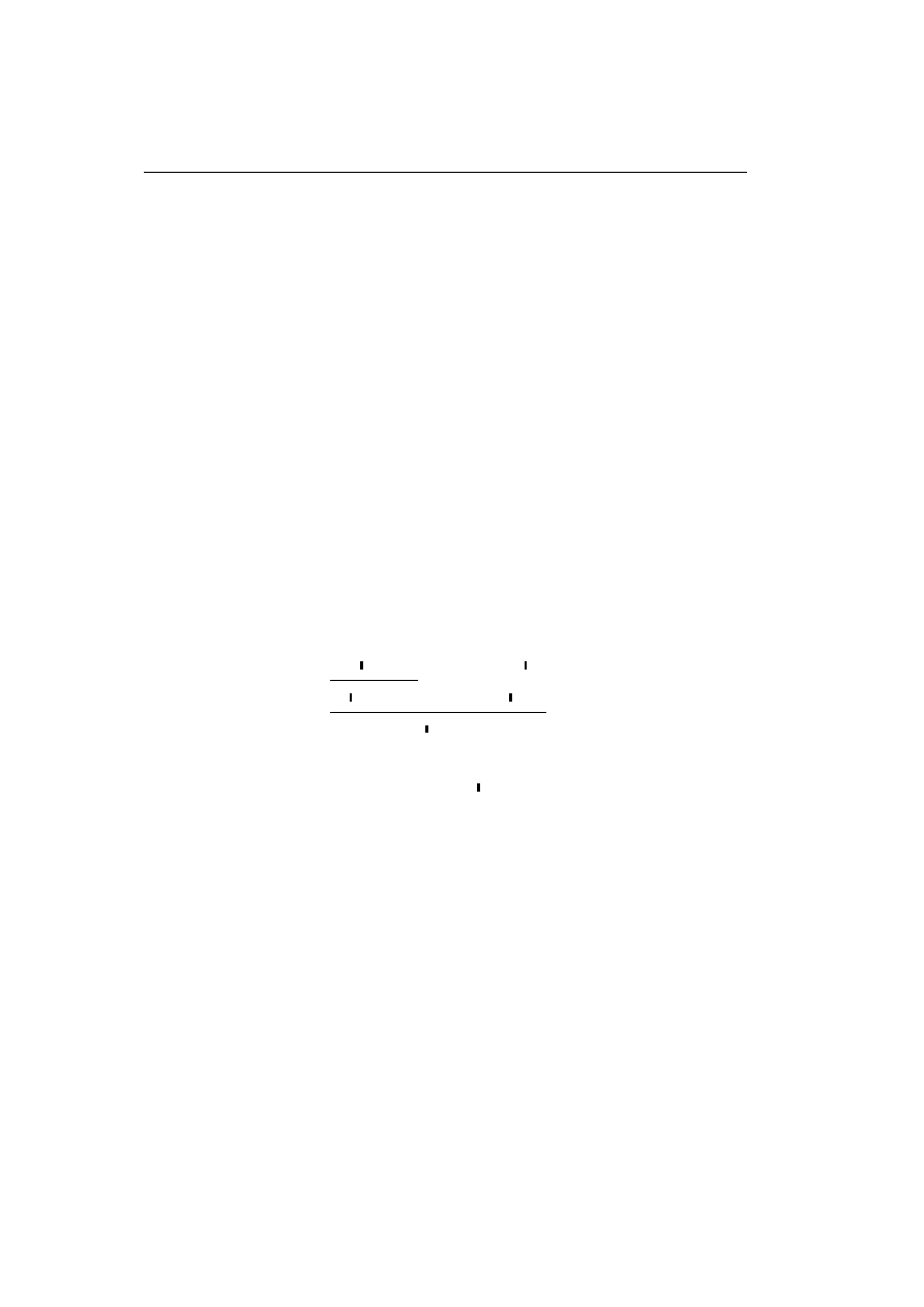
B.1.
Some Preliminary Results
of every situation where we have a cut such that the last rule of the left hand
side immediate subproof is the !
R
rule. The lemma is proved by induction
using the notion of height of a proof:
Definition B.1.2 The height h(τ ) of a proof τ is defined inductively as
follows:
1. if τ is an instance of a zero-premiss rule, then h(τ ) = 1,
2. if τ is obtained from the proof π by applying an instance of a one-
premiss rule, then h(τ ) = h(π) + 1,
3. if τ is obtained from the proofs π and π
0
by applying an instance of a
two-premiss rule, then h(τ ) = max
{h(π), h(π
0
)
} + 1.
Now the promised lemma.
Lemma B.1.3 Assume that !A
n
denotes a list of n occurrences of the for-
mula !A, and let a proof τ be given as follows
··
·
π
!Γ
− A, ?∆
!Γ
− !A, ?∆
··
· π
0
Γ
0
, !A
n
− ∆
0
========
Γ
0
, !A
− ∆
0
Γ
0
, !Γ
− ∆
0
, ?∆
where the subproofs π and π
0
have degrees strictly less than the degree of
τ . Then we can construct a proof of Γ
0
, !Γ
− ∆
0
, ?∆ which has degree strictly
less than the degree of τ
Proof: The proof is by induction on h(π
0
). In what follows, the last rule
used in π
0
is denoted by r
0
and we proceed on a case by case basis.
• r
0
is an instance of an axiom. We use the proof obtained by applying
!
R
to π.
• One of the n occurrences of the formula !A in the end-sequent of π
0
is
introduced by r
0
which is an instance of !
L
. We have two subcases. If
n = 1 then we have a (!
R
, !
L
) key-case which we change according to
the table of key-cases. If n > 1 then we have the following proof
49
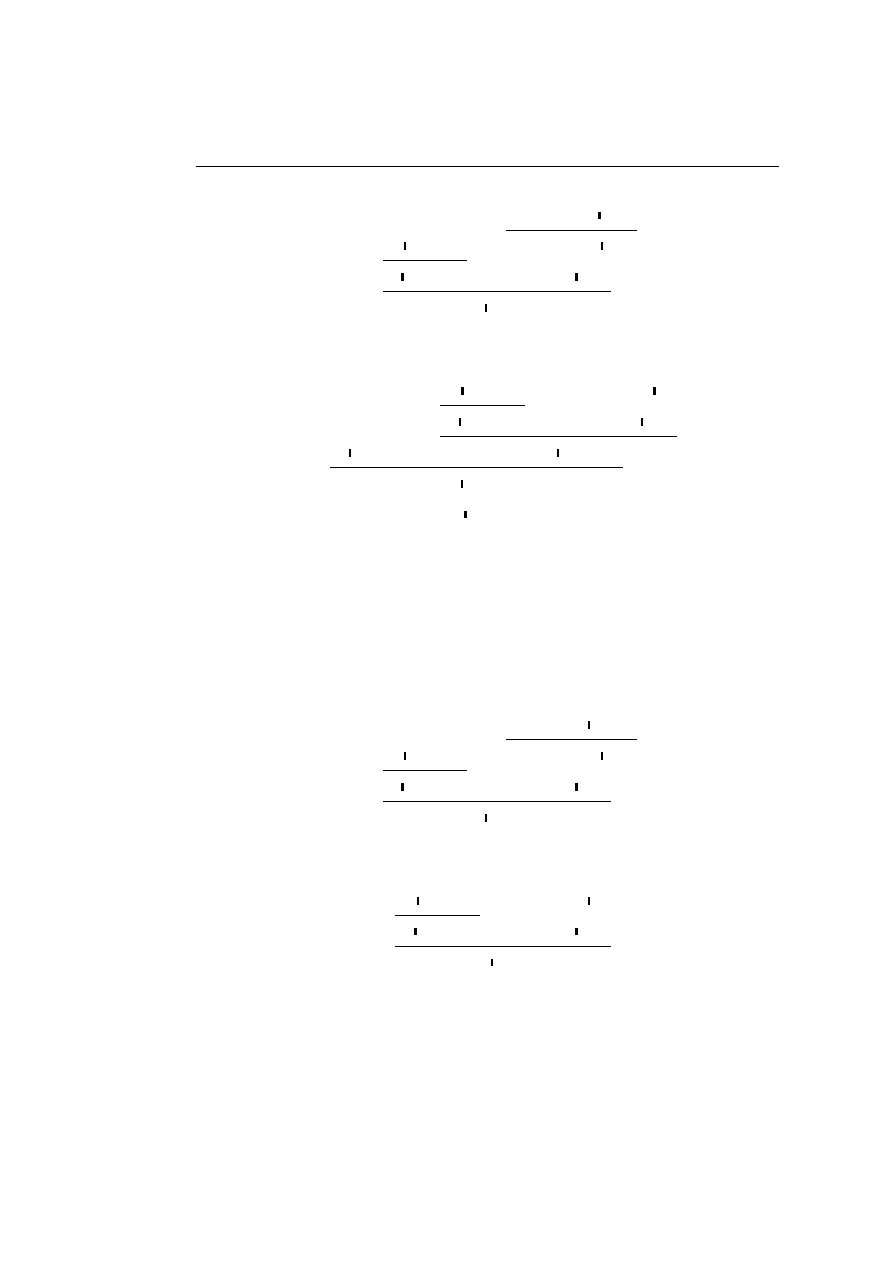
Appendix B.
Cut-Elimination for Classical Linear Logic
!Γ
− A, ?∆
!Γ
− !A, ?∆
Γ
0
, !A
n
−1
, A
− ∆
0
Γ
0
, !A
n
−1
, !A
− ∆
0
=============
Γ
0
, !A
− ∆
0
Γ
0
, !Γ
− ∆
0
, ?∆
which we transform into
!Γ
− A, ?∆
!Γ
− A, ?∆
!Γ
− !A, ?∆
Γ
0
, !A
n
−1
, A
− ∆
0
=============
Γ
0
, !A, A
− ∆
0
Γ
0
, !Γ, A
− ∆
0
, ?∆
Γ
0
, !Γ, !Γ
− ∆
0
, ?∆, ?∆
=================
Γ
0
, !Γ
− ∆
0
, ?∆
on which we apply the induction hypothesis on the appropriate sub-
proof.
• One of the n occurrences of the formula !A in the end-sequent of π
0
is
introduced by r
0
which is an instance of W
L
. We have two subcases. If
n = 1 then we have a (!
R
, W
L
) key-case which we change according to
the table of key-cases. If n > 1 then we have the following proof
!Γ
− A, ?∆
!Γ
− !A, ?∆
Γ
0
, !A
n
−1
− ∆
0
Γ
0
, !A
n
−1
, !A
− ∆
0
=============
Γ
0
, !A
− ∆
0
Γ
0
, !Γ
− ∆
0
, ?∆
which we transform into
!Γ
− A, ?∆
!Γ
− !A, ?∆
Γ
0
, !A
n
−1
− ∆
0
===========
Γ
0
, !A
− ∆
0
Γ
0
, !Γ
− ∆
0
, ?∆
on which we apply the induction hypothesis.
50
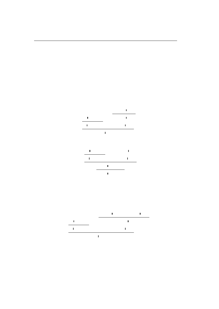
B.1.
Some Preliminary Results
• One of the n occurrences of the formula !A in the end-sequent of π
0
is introduced by r
0
which is an instance of C
L
. We apply the induc-
tion hypothesis to the immediate subproof of π
0
where we consider the
appropriate n + 1 occurrences of !A.
• None of the n occurrences of the formula !A in the end-sequent of π
0
are
introduced by r
0
. We have two subcases. In the first subcase all of the
n occurrences of the formula !A in the end-sequent of π
0
are inherited
from the same immediate subproof. If r
0
is a one-premiss rule, we have
the following proof
!Γ
− A, ?∆
!Γ
− !A, ?∆
Γ
1
, !A
n
− ∆
1
r
0
Γ
0
, !A
n
− ∆
0
=========
Γ
0
, !A
− ∆
0
Γ
0
, !Γ
− ∆
0
, ?∆
which we transform into
!Γ
− A, ?∆
!Γ
− !A, ?∆
Γ
1
, !A
n
− ∆
1
==========
Γ
1
, !A
− ∆
1
Γ
1
, !Γ
− ∆
1
, ?∆
r
0
Γ
0
, !Γ
− ∆
0
, ?∆
on which we apply the induction hypothesis on the appropriate sub-
proof. The situation is analogous if r
0
is a two-premiss rule. In the
second subcase the n occurrences of the formula !A in the end-sequent
of π
0
are not inherited from the same immediate subproof, so we have
the following proof
!Γ
− A, ?∆
!Γ
− !A, ?∆
Γ
1
, !A
p
− ∆
1
Γ
2
, !A
q
− ∆
2
r
0
Γ
0
, !A
p+q
− ∆
0
===========
Γ
0
, !A
− ∆
0
Γ
0
, !Γ
− ∆
0
, ?∆
which we transform into
51
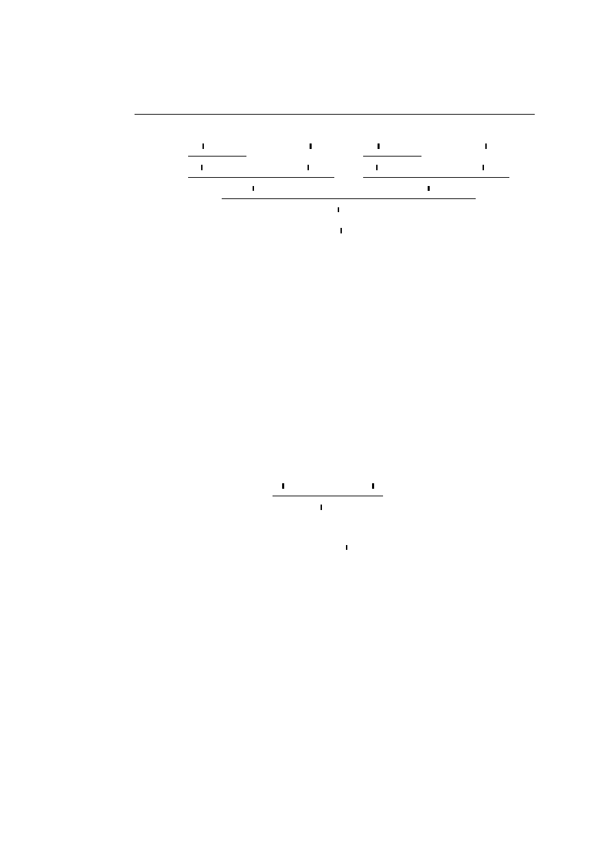
Appendix B.
Cut-Elimination for Classical Linear Logic
!Γ
− A, ?∆
!Γ
− !A, ?∆
Γ
1
, !A
p
− ∆
1
==========
Γ
1
, !A
− ∆
1
Γ
1
, !Γ
− ∆
1
, ?∆
!Γ
− A, ?∆
!Γ
− !A, ?∆
Γ
2
, !A
q
− ∆
2
=========
Γ
2
, !A
− ∆
2
Γ
2
, !Γ
− ∆
2
, ?∆
r
0
Γ
0
, !Γ, !Γ
− ∆
0
, ?∆, ?∆
=================
Γ
0
, !Γ
− ∆
0
, ?∆
on which we use the induction hypothesis on the appropriate two sub-
proofs.
2
There is a dual to Lemma B.1.3; and it is the case that the proofs are also
dual.
B.2
Putting the Proof Together
The following lemma is the engine of the cut-elimination proof.
Lemma B.2.1 Let a proof τ be given as follows
··
·
π
Γ
− A, ∆
··
·
π
0
Γ
0
, A
− ∆
0
Γ
0
, Γ
− ∆
0
, ∆
where the subproofs π and π
0
have degrees strictly less than the degree of τ .
Then we can construct a proof of Γ
0
, Γ
− ∆
0
, ∆ which has a degree strictly
less than the degree of τ .
Proof: Induction on h(π) + h(π
0
). In what follows, the last rules in π and
π
0
are denoted by r and r
0
, respectively, and the immediate subproofs of π
and π
0
are denoted by π
i
and π
0
j
, respectively. The formula A is denoted the
principal formula. We proceed case by case.
• r is an instance of an axiom; we use π
0
.
• r
0
is an instance of an axiom; dual to the previous case.
52
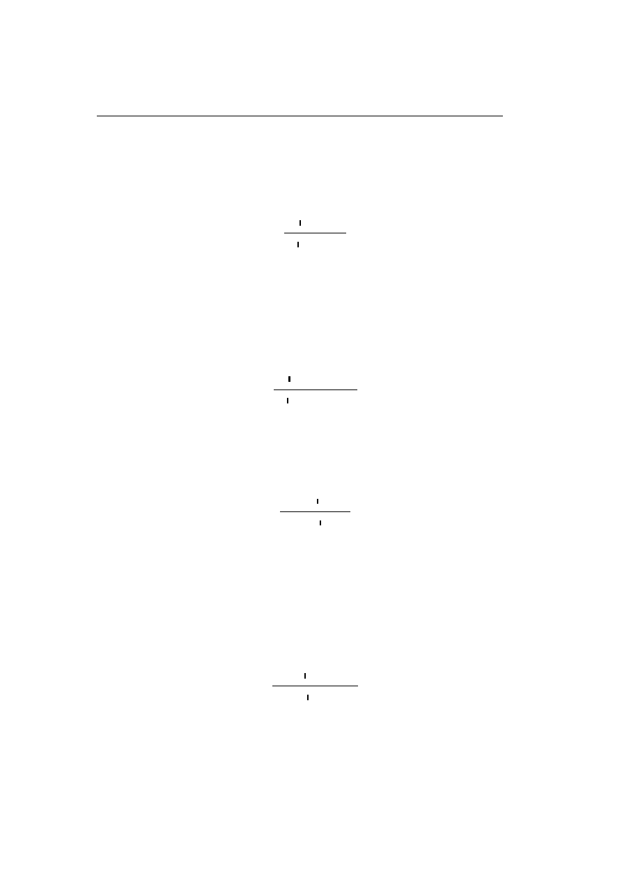
B.2.
Putting the Proof Together
We have now dealt with the cases where r or r
0
is an instance of an axiom.
• r is an instance of !
R
that introduces the principal formula; thus, A =!A
0
for some A
0
, and π looks as follows:
!Γ
− A
0
, ?∆
!Γ
− !A
0
, ?∆
We use Lemma B.1.3.
• r
0
is an instance of ?
L
that introduces the principal formula; dual to
the previous case.
• r is an instance of !
R
that does not introduce the principal formula;
thus, A =?A
0
for some A
0
, and π looks as follows:
!Γ
− B, ?A
0
, ?∆
!Γ
− !B, ?A
0
, ?∆
If the principal formula ?A
0
is not introduced by r
0
, then we push π
upwards in the right hand side subproof (note that r
0
cannot be an
instance of !
R
or ?
L
) and use the induction hypothesis. If the principal
formula ?A
0
is introduced by r
0
, that is, π
0
looks as follows:
!Γ
0
, A
0
− ?∆
0
!Γ
0
, ?A
0
− ?∆
0
then we push π
0
upwards in the left hand side subproof (note that each
formula in !Γ
0
has a ! at the top level and each formula in ?∆
0
has a ?
at the top level) and use the induction hypothesis.
• r
0
is an instance of ?
L
that does not introduce the principal formula;
dual to the previous case.
• r is an instance of ?
L
; thus, A =?A
0
for some A
0
, and π looks as follows:
!Γ, B
− ?A
0
, ?∆
!Γ, ?B
− ?A
0
, ?∆
53

Appendix B.
Cut-Elimination for Classical Linear Logic
If the principal formula ?A
0
is not introduced by r
0
, then we push π
upwards in the right hand side subproof (note that r
0
cannot be an
instance of !
R
or ?
L
) and use the induction hypothesis. If the principal
formula ?A
0
is introduced by r
0
, that is, π
0
looks as follows:
!Γ
0
, A
0
− ?∆
0
!Γ
0
, ?A
0
− ?∆
0
then we push π
0
upwards in the left hand side subproof (note that each
formula in !Γ
0
has a ! at the top level and each formula in ?∆
0
has a ?
at the top level) and use the induction hypothesis.
• r
0
is an instance of !
R
; dual to the previous case.
We have now dealt with the cases where r or r
0
is an instance of !
R
or ?
L
.
• r does not introduce the principal formula; we push π
0
upwards in the
left hand side subproof and use the induction hypothesis.
• r
0
does not introduce the principal formula; dual to the previous case.
• r introduces the principal formula on the right hand side and r
0
intro-
duces the principal formula on the left hand side; we have a (
⊗
R
,
⊗
L
),
(I
R
, I
L
), (
.............................
......
..
............
...........
....
...
...
....
............
.........
R
,
.............................
......
..
............
...........
....
..
..
..
....
............
.........
L
), (
⊥
R
,
⊥
L
) or (
(
R
,
(
L
) key-case. We change τ ac-
cording to the table of key-cases.
2
Lemma B.2.2 Given a proof τ of the sequent Γ
− ∆ we can construct a
proof of the same sequent with degree strictly lower than the degree of τ .
Proof: Induction on h(τ ). If the last rule used in τ is not a cut with the
same degree as the degree of τ , we are done by using the induction hypothesis
on the immediate subproofs of τ . If the last rule in τ is a cut with the same
degree as the degree of τ , we apply the induction hypothesis on the immediate
subproofs of τ , and obtain a proof τ
0
which looks as follows
54

B.2.
Putting the Proof Together
··
·
π
Γ
0
− A, ∆
0
··
·
π
0
Γ
00
, A
− ∆
00
Γ
00
, Γ
0
− ∆
00
, ∆
0
where the proofs π and π
0
have degrees strictly lower than the degree of
τ
0
. Note that Γ
00
, Γ
0
is equal to Γ and ∆
00
, ∆
0
is equal to ∆. We then use
Lemma B.2.1.
2
And now the Hauptsatz.
Theorem B.2.3 Given any proof of a sequent we can construct a cut-free
proof of the same sequent.
Proof: Iteration of Lemma B.2.2.
2
55

Recent Publications in the BRICS Lecture Series
LS-96-6 Torben Bra ¨uner. Introduction to Linear Logic. December
1996. iiiv+55 pp.
LS-96-5 Devdatt P. Dubhashi. What Can’t You Do With LP? De-
cember 1996. viii+23 pp.
LS-96-4 Sven Skyum. A Non-Linear Lower Bound for Monotone
Circuit Size. December 1996. viii+14 pp.
LS-96-3 Kristoffer H. Rose. Explicit Substitution – Tutorial & Sur-
vey. September 1996. v+150 pp.
LS-96-2 Susanne Albers. Competitive Online Algorithms. Septem-
ber 1996. iix+57 pp.
LS-96-1 Lars Arge.
External-Memory Algorithms with Applica-
tions in Geographic Information Systems. September 1996.
iix+53 pp.
LS-95-5 Devdatt P. Dubhashi.
Complexity of Logical Theories.
September 1995. x+46 pp.
LS-95-4 Dany Breslauer and Devdatt P. Dubhashi. Combinatorics
for Computer Scientists. August 1995. viii+184 pp.
LS-95-3 Michael I. Schwartzbach. Polymorphic Type Inference.
June 1995. viii+24 pp.
LS-95-2 Sven Skyum. Introduction to Parallel Algorithms. June
1995. viii+17 pp. Second Edition.
LS-95-1 Jaap van Oosten. Basic Category Theory. January 1995.
vi+75 pp.
Wyszukiwarka
Podobne podstrony:
Wavelet Transforms that Map Integers to Integers [jnl article] (1996) WW
Bayesian Methods A General Introduction [jnl article] E Jaynes (1996) WW
An Introduction to Conformal Field Theory [jnl article] M Gaberdiel (1999) WW
Introduction to Stochastic Calculus for Finance D Sondermann (Springer, 2006) WW
An Introduction to Statistical Inference and Data Analysis M Trosset (2001) WW
Introduction to Smooth Manifolds [Errata] J Lee (2000) WW
An Introduction to the Theory of Numbers L Moser (1957) WW
Introduction to VHDL
268257 Introduction to Computer Systems Worksheet 1 Answer sheet Unit 2
Introduction To Scholastic Ontology
Evans L C Introduction To Stochastic Differential Equations
Zizek, Slavoj Looking Awry An Introduction to Jacques Lacan through Popular Culture
Introduction to Lagrangian and Hamiltonian Mechanics BRIZARD, A J
Introduction to Lean for Poland
An Introduction to the Kabalah
Introduction to Apoptosis
więcej podobnych podstron