
WAVELET TRANSFORMS THAT MAP INTEGERS TO INTEGERS
A. R. CALDERBANK, INGRID DAUBECHIES, WIM SWELDENS, AND BOON-LOCK YEO
August 1996
Abstract.
Invertible wavelet transforms that map integers to integers have important appli-
cations in lossless coding. In this paper we present two approaches to build integer to integer
wavelet transforms. The first approach is to adapt the precoder of Laroia et al., which is used in
information transmission; we combine it with expansion factors for the high and low pass band
in subband filtering. The second approach builds upon the idea of factoring wavelet transforms
into so-called lifting steps. This allows the construction of an integer version of every wavelet
transform. Finally, we use these approaches in a lossless image coder and compare the results
to the literature.
1. Introduction
Wavelets, wavelet packets, and local cosine transforms are used in a variety of applications,
including image compression [2, 29, 39, 10, 25]. In most cases, the filters that are used have
floating point coefficients. For instance, if one prefers to use orthonormal filters with an assigned
number N (N
>
2) of vanishing moments and minimal filter length, then the resulting filter
coefficients are real numbers which can be computed with high precision, but for which we do
not even have a closed form expression if N > 3 [8]. When the input data consist of sequences
of integers (as is the case for images), the resulting filtered outputs no longer consist of integers.
Yet, for lossless coding it would be of interest to be able to characterize the output completely
again with integers.
In the case of the Fourier and cosine transforms, this problem has been solved in [17]. An
integer version of the orthogonal Haar transform has been known for some time as the S-
transform [24, 16]. In [10] a redundant integer version of the Haar transform is introduced
which uses rounded integer arithmetic and which yields near optimal approximation in certain
Besov spaces. Relaxing the constraint of orthonormality of the wavelets makes it possible to
obtain filter coefficients that are dyadic rationals [6, 14, 37, 31]; up to scaling these filters can
be viewed as mapping integers to integers. This rescaling amplifies the dynamic range of the
1991 Mathematics Subject Classification. 42C15, 94A29.
Key words and phrases. wavelet, lossless compression, integer transforms, precoding, lifting, source coding.
1

data considerably, however, so that this does not lead to reasonable lossless compression. In the
special case of binary valued images it is possible to define binary valued wavelet transforms
(and thus no bit growth) [18, 31].
In this paper, we present two approaches that lead to wavelet transforms that map integers
to integers, and which can be used for lossless coding. The two approaches are independent
of each other, and the reader can explore the corresponding two parts of this paper (Section 2
and Section 3) in either order. The second approach looks more promising for lossless image
coding. Note that in both cases we are not building integer arithmetic wavelet transforms. Thus
the computations are still done with floating point numbers, but the result is guaranteed to be
integer and invertibility is preserved. In software applications, this should not affect speed, as in
many of today’s microprocessors floating point and integer computations are virtually equally
fast.
The first approach, in Section 2, is inspired by the precoding invented by Laroia, Tretter,
and Farvardin (LTF) [21], which is used for transmission over channels subject to intersymbol
interference and Gaussian noise. When integer data undergo causal filtering with a leading filter
coefficient equal to 1, this precoding makes small (non-integer) adjustments to the input data
resulting in integer outputs after filtering. In Section 2.1, we try to adapt this method to the
subband filtering inherent to a wavelet transform. Even though this approach cannot be made
to work for other wavelet bases than the Haar basis, it leads to a reformulation of the original
problem, by including the possibility of an expansion coefficient. Section 2.2 shows how the
specific structure of wavelet filters can be exploited to make this expansion coefficient work. In
Section 2.3, we generalize the expansion idea to propose different expansion factors for the low
and the high pass filter: for the high pass filter, we can afford a larger expansion factor because
the dynamic range of its output tends to be smaller anyway. In most cases, the product of the
expansion factors for high and low pass is larger than 1, which turns out to be bad for lossless
compression.
A different approach (although there are points of contact) is taken in Section 3. An example
in [39] of a wavelet transform that maps integers to integers is seen to be an instance of a
large family of similar transforms, obtained by combining the lifting constructions proposed in
[32, 33] with rounding-off in a reversible way. In Section 3.1 we review the S transform, and in
Section 3.2 two generalizations, the TS transform and the S+P transform. In Section 3.3 we
briefly review lifting, and in Section 3.4 we show how a decomposition in lifting steps can be
turned into an integer transform. In general, this transform exhibits some expansion factors as
well. Unlike to what happened in Section 2 the product of the low and high pass expansion
2

factors is now always equal to 1. Section 3.5 gives a short discussion of how this approach can
be linked to the one in Section 2. In Section 4, we show many examples.
Finally, in Section 5 we show applications of the two approaches to lossless image coding, and
we compare our results with other results in the literature.
Except where specified otherwise, our notations conform with the standard notations for filters
associated with orthonormal or biorthogonal wavelet bases, as found in e.g., [8].
2. Expansion factors and integer to integer transforms
2.1. Precoding for subband filtering. We start by reviewing briefly the LTF precoder [21].
Suppose we have to filter a sequence of integers (a
n
)
n∈Z
, with a causal filter (i.e., h
k
= 0 for
k < 0) and leading coefficient 1 (i.e., h
0
= 1). If the h
k
are not themselves integers, then the
filtered output b
n
= a
n
+
P
∞
k=1
h
k
a
n−k
will in general not consist of integers either. The LTF
precoder replaces the integers a
n
by non-integers a
0
n
by introducing small shifts r
n
, in such a
way that the resulting b
0
n
are integers. More concretely, define
a
0
n
= a
n
− r
n
r
n
=
(
∞
X
k=1
h
k
a
0
n−k
)
=
(
∞
X
k=1
h
k
(a
n−k
− r
n−k
)
)
,
where the symbol
{x} = x − bxc stands for the fractional part of x, and bxc for the largest
integer not exceeding x. In practice, both the a
n
and the h
k
are non-zero for only finite ranges
of the indices n or k, so that the infinite recursion is not a problem: if a
n
= 0 for n < 0, then
so are a
0
n
and r
n
and the recursion can be started. If we now compute b
0
n
= a
0
n
+
P
∞
k=1
h
k
a
0
n−k
,
then we immediately see that
b
0
n
= a
n
+
$
∞
X
k=1
h
k
a
0
n−k
%
is an integer. To recover the original a
n
from the b
0
n
, one first applies the inverse filter 1/H(z) =
(1 +
P
∞
k=1
h
k
z
k
)
−1
(assuming this filter is stable), which gives the a
0
n
from which
a
n
= a
0
n
+
(
∞
X
k=1
h
k
a
0
n−k
)
can be computed immediately.
3

This approach can also be used if h
0
6= 1. In that case, if we have
a
0
n
= a
n
− r
n
r
n
=
(
(h
0
− 1)a
0
n
+
∞
X
k=1
h
k
a
0
n−k
)
=
(
(h
0
− 1)(a
n
− r
n
) +
∞
X
k=1
h
k
a
0
n−k
)
,
(2.1)
then the
b
0
n
=
∞
X
k=0
h
k
a
0
n−k
= a
0
n
+
$
(h
0
− 1)a
0
n
+
∞
X
k=1
h
k
a
0
n−k
%
+ r
n
= a
n
+
$
(h
0
− 1)a
0
n
+
∞
X
k=1
h
k
a
0
n−k
%
are integers again. The situation is now slightly more complicated, because the r
n
are defined
implicitly. Since both a
n
and the a
0
n−k
for k
>
1 are known when r
n
needs to be determined, we
can reformulate (2.1) as
r
n
=
{(1 − h
0
)r
n
+ y
n
}
with y
n
=
(h
0
− 1)a
n
+
P
∞
k=1
h
k
a
0
n−k
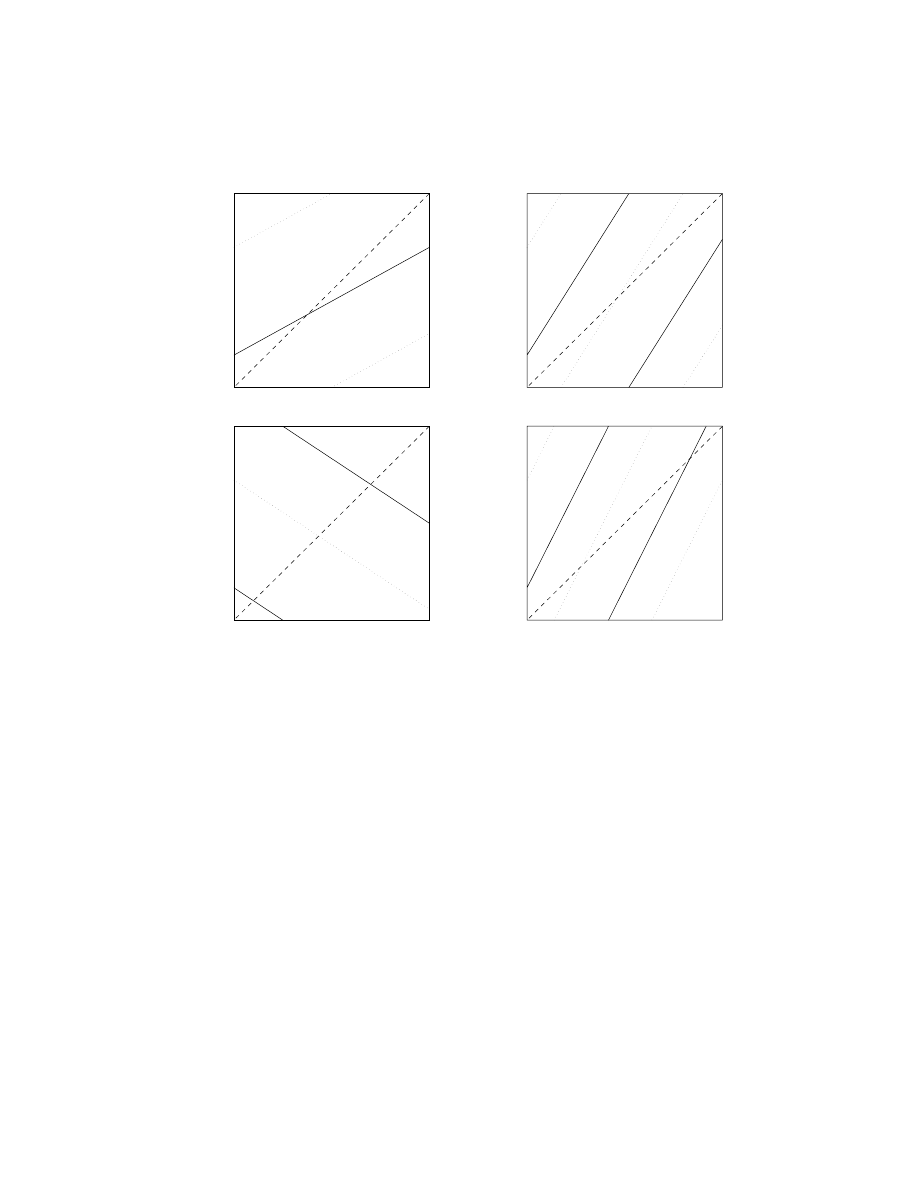
. Whether or not the equation
r =
{αr + y}
(2.2)
has a solution for arbitrary y
∈ [0, 1) depends on the size and sign of α. As shown in Figure 1,
a solution fails to exist for some choices of y if 0 < α < 2; for α
6
0 or α
>
2 there always exists
at least one solution. This range for α where (2.2) always has a solution corresponds to
|h
0
|
>
1.
When faced with having to use the precoder for cases where
|h
0
| < 1, a simple expedient is to
consider a renormalized filter, with e
h
n
= αh
n
, so that
|eh
0
|
>
1. (For instance, α = h
−1
0
will do.)
In the case of the wavelet transform, we work with several filters, followed by decimation.
In this paper, we shall always work with 2-channel perfect reconstruction filter banks; in this
section, unless specified explicitly, we assume the filter pair is orthonormal.
Assume that the two filters H and G are FIR, with h
n
= g
n
= 0 if n < 0 or n
>
2N . Then
we have
s
1,n
=
X
k
h
2n−k
s
0,k
d
1,n
=
X
k
g
2n−k
s
0,k
,
(2.3)
4
0
1
1
0
1
1
1
1
1
0
1
y2
0
r
r
r
r
y2
y1
y2
y1
y1
y2
y1
a
c
d
b
Figure 1.
Solving r =
{αr + y}:
a: For 0 < α
6
1, the equation r =
{αr + y} has solutions for y = y
1
(full) but
not for y = y
2
(dotted), since
{αr + y
1
} intersects the diagonal (dashed), but
{αr + y
2
} does not.
b: For 1
6
α < 2, the situation is reversed.
c: For α
6
0 we always have at least one solution.
d: Likewise for α
>
2.
which can be rewritten as
s
1,n
d
1,n
!
=
X
k
h
2(n−k)
h
2(n−k)+1
g
2(n−k)
g
2(n−k)+1
!
s
0,2k
s
0,2k−1
!
=
N
X
k=0
h
2k
h
2k+1
g
2k
g
2k+1
!
s
0,2(n−k)
s
0,2(n−k)−1
!
(2.4)
(This corresponds to a polyphase decomposition of the filters; see e.g., [30, 35, 38].) The sub-
scripts 0, 1 correspond to the “level” of the filtered sequences; level 0 are the unprocessed data,
5

while level 1 corresponds to one application of the H, G filters. More generally, s
j,n
and d
j,n
are
obtained by applying H, G to the s
j−1,k
, so that they are the results of j layers of filters.
If we define
H
k
=
h
2k
h
2k+1
g
2k
g
2k+1
!
with 0
6
k
6
N
− 1 ,
then (2.4) can be read as a 2D analog to the situation above; now each a
n
or b
n
is a 2-vector, with
a
n
= (s
0,2n
s
0,2n−1
)
t
, and b
n
= (s
1,n
d
1,n
)
t
. For an arbitrary 2-vector a = (a
1
a
2
)
t
, we introduce
the notations
{a} =
{a
1
}
{a
2
}
!
, and
bac =
ba
1
c
ba
2
c
!
.
We can now generalize the LTF precoder by defining
a
0
n
= a
n
− r
n
r
n
=
(
(H
0
− I)a
0
n
+
N −1
X
k=1
H
k
a
0
n−k
)
=
{(I − H
0
)r
n
+ y
n
} ,
(2.5)
with
y
n
=
(
(H
0
− I)a
n
+
N −1
X
k=1
H
k
a
0
n−k
)
.
If the equations (2.5) for r
n
can indeed be solved, then we find, as before, that the
b
0
n
=
n−1
X
k=0
H
k
a
0
n−k
consist of only integer entries. It is not clear, however, that the equation
r =
{(I − H
0
)r + y
}
(2.6)
always has solutions for any y
∈ [0, 1) × [0, 1). Indeed, for the Haar case, where
H
0
=
1
√
2
1
√
2
−
1
√
2
1
√
2
!
one checks that (2.6) has no solution if y
1
= 1/4, y
2
= 1/2.
The simple expedient of “renormalizing” H
0
to αH
0
works here as well. Let us replace the
orthonormal filtering (2.3) and its inverse
s
0,k
=
X
n
[h
2n−k
s
1,n
+ g
2n−k
d
1,n
]
6

by scaled versions:
es
1,n
= α
X
k
h
2n−k
s
0,k
,
e
d
1,n
= β
X
k
g
2n−k
s
0,k
s
0,k
=
X
n
h
α
−1
h
2n−k
es
1,n
+ β
−1
g
2n−k
e
d
1,n
i
.
The polyphase regrouping then uses the matrices
e
H
k
=
αh
2k
αh
2k+1
βg
2k
βg
2k+1
!
=
α
0
0
β
!
H
k
;
the corresponding equations for r
1
, r
2
become
r
1
=
{(1 − αh
0
)r
1
+ (y
1
− αh
1
r
2
)
}
r
2
=
{(1 − βg
1
)r
2
+ (y
2
− βg
0
r
1
)
} .
(2.7)
For the special case where the wavelet basis is the Haar basis, i.e., h
0
= h
1
=
1
√
2
= g
1
=
−g
0
,
with all other h
n
, g
n
= 0, we can choose α = β =
√
2. The system for r
1
, r
2
reduces then to
r
1
=
{y
1
− r
2
}
r
2
=
{y
2
+ r
1
}
which has the easy solution r
1
=
{(y
1
− y
2
)/2
} , r
2
=
{(y
1
+ y
2
)/2
} for arbitrary y
1
, y
2
∈ [0, 1).
Unfortunately, things are not as easy for orthonormal wavelet filters of higher order. When
N > 1, orthonormality of the wavelet filters implies
h
2N−2
g
0
+ h
2N−1
g
1
= 0
h
2N−2
h
0
+ h
2N−1
h
1
= 0 ,
where h
2N−1
6= 0. Hence h
0
g
1
=
−h
2N−2
g
0
h
0
/h
2N−1
= h
1
g
0
or det H
0
= 0.
This implies that
r =
{(I − αH
0
)r + y
}
(2.8)
cannot be solved for arbitrary y
∈ [0, 1)
2
, regardless of the choice of α, as shown by the following
argument. Suppose that for a given y in the interior of [0, 1)
2
, r solves (2.8). Then there exists
n
∈ Z
2
so that
r + n = (I
− αH
0
)r + y ,
or αH
0
r + n = y. Since both r and y are in [0, 1)
2
, it follows that
knk is bounded by some C > 0,
uniformly in y. Since det H
0
= 0, there exists a 2-vector e in R
2
so that αH
0
R
2
⊂ {λe; λ ∈ R}.
7

Take now f
⊥e, and consider y
0
= y + µf . Since y was chosen in the interior of [0, 1)
2
, y
0
still
lies within [0, 1)
2
for sufficiently small µ. Suppose r
0
is the corresponding solution of (2.8),
αH
0
r
0
+ n
0
= y
0
= y + µf .
Taking inner products of both sides with f leads to
hn
0
, f
i = hy, fi + µkfk
2
,
or
µ =
hn
0
− y, fi/kfk
2
.
Since the right hand side can take on only a finite set of values (since n
0
∈ Z
2
,
kn
0
k
6
C), this can
only hold for finitely many values of µ, and not for the interval around 0 for which y
0
= y + µf
is within [0, 1)
2
. (Note that the same no-go argument still works if we replace α by a diag-
onal matrix A, corresponding to a non-uniform expansion; in that case it suffices to choose
f
⊥ AH
0
R
2
.)
There exists a way around this problem, which exploits that the y
n
are not really independent
of the a
n
or r
n
, as we have implicitly assumed here. This is the subject of the next subsection.
2.2. Uniform expansion factors. For the Haar filter, we were looking in the last subsection
at the equation
y
1
y
2
!
=
n
1
n
2
!
+ α
1
√
2
1
√
2
−
1
√
2
1
√
2
!
r
1
r
2
!
For α = 1, n
1
, n
2
∈ Z and r
1
, r
2
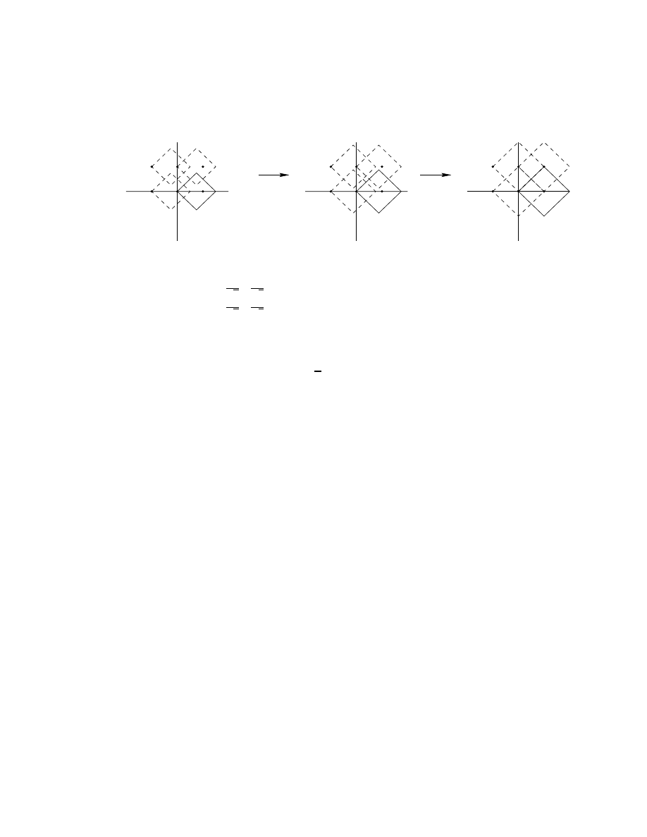
∈ [0, 1), the possible values taken on by the right hand side
range over the union of tilted squares shown in Figure 2a, which clearly do not cover the square
[0, 1)
2
. For α =
√
2, the tilted squares are blown up so that their union does not leave any gaps.
In the Haar case, the different pairs (s
0,2k
, s
0,2k−1
) remain nicely decoupled in the subband
filtering process, which enabled us to reduce the whole analysis to a 2D argument. As we saw
above, the most naive way to reduce to 2D does not work for longer filters; a solution to the
problem at the end of the last section is possible only by taking into account to some extent
the coupling between the pairs (s
0,2k
, s
0,2k−1
) in the filtering process. To do this, we shall first
consider the full problem, for the complete data sequence, and try to carry out a reduction to
fewer dimensions at a later stage. Imagine that the initial data constitute a finite sequence
(of length L) of integers, a
∈ Z
L
. The subband filtering operator H can now be viewed as an
8
c
a
b
(1,0)
(1,1)
(0,0)
(-1,0)
(0,1)
(-1,1)
Figure 2.
a. For H
0
=
1
√
2
1
√
2
−
1
√
2
1
√
2
!
, the union
S
n∈Z
2
(H
0
[0, 1)
2
+ n) does not cover
[0, 1)
2
.
b. and c. As α
>
1 increases, the set [0, 1)
2
\
S
n∈Z
2
(αH
0
[0, 1)
2
+ n) becomes
smaller; the gap closes for α =
√
2.
L
× L-matrix, which decomposes into 2 × 2 blocks (see Section 2.1).
H =
H
0
H
1
H
2
· · · H
N −3
H
N −2
H
N −1
0
0
· · ·
0
0
H
0
H
1
· · · H
N −4
H
N −3
H
N −2
H
N −1
0
· · ·
0
..
.
..
.
..
.
..
.
..
.
..
.
..
.
..
.
..
.
..
.
..
.
H
1
H
2
H
3
· · · H
N −2
H
N −1
0
0
0
· · · H
0
(2.9)
(We have here given H a circulant-structure to deal with the finite length of the data sequence,
which amounts to periodizing the data. Other ways of extending the data, such as reflections
or interpolation techniques, can also be used. This would change only the first and last few
rows and columns of the matrix, and it would not affect our argument significantly, although we
would, of course, have to take those changes into account near the start and end of the signal.
We have also implicitly assumed that L is even here, which is usually the case; odd L can be
handled as well, but are slightly more tricky.)
In general, Ha
6∈ Z
L
if a
∈ Z
L
. An appropriate shift of Ha will bring it back to Z
L
. More pre-
cisely, if Λ is a fundamental region in R
L
for the lattice Z
L
, then we can find f = f (a)
∈ Λ so that
Ha + f
∈ Z
L
. In order for the transform a
−→ Ha + f(a) to be invertible, we must require that
if a
6= a
0
, then Ha + f (a)
6= Ha
0
+ f (a
0
), or since H itself is invertible, H
−1
f (a)
6= H
−1
f (a
0
) + (a
0
− a).
This will be satisfied if H
−1
Λ
T
(H
−1
Λ + n) =
∅ for n ∈ Z
L
, n
6= 0. The Haar example shows us
already that it may not be possible to find such a fundamental region Λ without introducing an
9

expansion factor. (For Haar, the problem reduces to considering H
0
only in 2D; since H
−1
0
= H
t
0
,
we can look at Figure 2a again, which shows the regions H
0
[0, 1)
2
+ n; their mirror images are
the H
t
0
[0, 1]
2
+ m. For α = 1, they do intersect non-trivially.) If we do use an expansion factor
α, then we are dealing with the transform a
−→ αHa + f instead, and the sufficient condition
for invertibility becomes
H
−1
(α
−1
Λ)
\
H
−1
(α
−1
Λ + n) =
∅ for all n ∈ Z
L
\∅ .
(2.10)
(In this section we consider uniform dilation factors only; non-uniform dilations, with different
expansion factors for high and low pass parts, will be considered in the next subsection.) Given
any bounded fundamental region Λ, (2.10) will always be satisfied for sufficiently large α; the
challenge is, for a given H, to find a “reasonable” Λ for which α is as small as possible. (Since
one goal of this approach is to develop a practical lossless coding scheme with wavelets, the
region Λ must be tractable for numerical computations. In the Haar case of last section, we had
Λ = [0, 1)
L
, and α =
√
2.) It will be useful below, when we try to construct explicit Λ, to relax
the condition that Λ be exactly a fundamental region and to require instead that Λ contain a
fundamental region. Renaming α
−1
Λ = Γ, we have therefore the following challenge:
Find Γ
⊂ R
N
so that
• αΓ contains a fundamental region for Z
L
(with α
>
1 as small as we can get it)
• for all n ∈ Z
L
, n
6= 0.
H
−1
Γ
\
(H
−1
Γ + n) =
∅ .
(2.11)
In order to reduce the problem to a smaller size and make the search for a suitable Γ more
tractable, we shall here restrict ourselves to special Γ of the form
Γ = Ω
× Ω × . . . × Ω ,
where Ω
⊂ R
2
so that αΩ contains a fundamental region for Z
2
. This still enables us to exploit
the 2
× 2-block structure of H. Moreover, this will also make the implementation easier. Instead
of working with the large matrix H and its inverse, for which we would have to wait to acquire
all the data, restricting ourselves to product Γ makes a “running” implementation possible.
Let us look at this problem for the simplest example beyond the Haar case, which uses the
4-tap filters
h
0
=
1+
√
3
4
√
2
,
h
1
=
3+
√
3
4
√
2
,
h
2
=
3−
√
3
4
√
2
,
h
3
=
1−
√
3
4
√
2
,
g
0
=
−h
3
,
g
1
= h
2
,
g
2
=
−h
1
,
h
3
= h
0
.
10

Introducing the unitary matrices
U =
1
2
√
2
1 +
√
3
1
−
√
3
√
3
− 1 1 +
√
3
!
V =
1
2
1
√
3
−
√
3
1
!
,
we can rewrite the matrices H
0
and H
1
(the only non-zero H
k
) in this case as
H
0
= U
1
0
0
0
!
V = U e
H
0
V,
H
1
= U
0
0
0
1
!
V = U e
H
1
V .
(This is in fact a different way of writing the factorization of [36] for this particular case.)
It follows that H = U e
HV, where U and V are matrices with the 2
× 2 blocks U resp. V , on
the diagonal, and zeros elsewhere, and where
e
H =
e
H
0
e
H
1
0
· · ·
0
0
e
H
0
e
H
1
· · ·
0
..
.
..
.
e
H
1
0
0
· · ·
e
H
0
=
1
0
0
0
0
0
· · · · · · 0 0
0
0
0
1
0
0
· · · · · · 0 0
0
0
1
0
0
0
· · · · · · 0 0
0
0
0
0
0
1
· · · · · · 0 0
..
.
..
.
..
.
..
.
..
.
..
.
..
.
..
.
..
.
..
.
..
.
..
.
..
.
..
.
..
.
..
.
0
0
0
0
0
0
· · · · · · 1 0
0
1
0
0
0
0
· · · · · · 0 0
.
Note that e
Hf (and therefore e
H
−1
f as well) is just a permutation of the even entries of f .
(For longer filters H this will no longer be true; we shall see below how to extend this ap-
proach to that case.) It follows that if e
Γ is a product of 2D regions, e
Γ = e
Ω
× . . . × eΩ, with
eΩ ⊂ [a
1
, a
2
)
× [b
1
, b
2
) = R then e
He
Γ
⊂ R × . . . × R. In particular, any eΓ that is already of the
form R
× . . . × R is invariant under e
H or e
H
−1
. This suggests the following strategy for find-
ing a suitable Ω that would satisfy all our requirements. Take Ω so that U
t
Ω is a rectangle
with its sides parallel to the axes; then U
t
Γ = U
t
Ω
× . . . × U
t
Ω will be left invariant by e
H,
so that H
−1
Γ = (V
t
U
t
Ω
× . . . × V
t
U
t
Ω), and our sufficient condition reduces to a set of 2D
requirements. In particular, the last part (2.11) of the sufficient condition reduces to
V
t
U
t
Ω
\
(V
t
U
t
Ω + n) =
{0} for n ∈ Z
2
\{0} .
Since U
t
Ω = [a
1
, a
2
)
× [b
1
, b
2
) = R, this can be rewritten as
R
\
(R + V n) =
{0} for n ∈ Z
2
\{0}
11

or
R
− R
\
V Z
2
=
{0} ,
where we have used the notation A
− B = {x − y; x ∈ A, y ∈ B}; in our case both A and B
equal R, and
R
− R = {x − y; x, y ∈ R}
=
{z = (u, v); |u| < a
2
− a
1
,
|v| < b
2
− b
1
} .
Note that this set is symmetric around the origin, even if R is not. We can therefore assume,
without loss of generality, that R is centered around the origin, so that the condition reduces to
2R
◦
\
V Z
2
=
{0} or 2(V
t
R)
◦
\
Z
2
=
{0} ,
where B
◦
denotes the interior of the set B.
In summary, we are thus looking for a rectangle R
a,b
= [
−a, a) × [−b, b) so that
• αUR
a,b
contains a fundamental region for Z
2
• 2(V
t
R
a,b
)
◦
T
Z
2
=
{0}.
We would like to find a, b so that α is as small as possible. We start by constructing one
candidate for R
a,b
, and computing the corresponding α. The following technical lemma will be
useful in our construction:
Lemma 2.1. Start with a parallelogram P that is a fundamental region for Z
2
in R
2
. Form a
hexagon ∆
⊂ P by picking six points on the boundary of P so that opposite vertices are congruent
modulo Z
2
and so that no three of the six points are collinear. Then any parallelogram e
P that
contains ∆ also contains the interior of a fundamental region of Z
2
.
Proof. See Appendix A.
(Note that as a fundamental region for Z
2
, P cannot be open nor closed. Likewise, e
P can fail
to contain a true fundamental region if e
P contains too little of ∂ e
P .)
Corollary 2.2. Any parallelogram symmetric around 0 that contains the points (
1
2
, 0), (0,
1
2
) and
either (
1
2
,
1
2
) or (
1
2
,
−
1
2
) contains the interior of a fundamental region for Z
2
.
Let us apply this to our problem. We start with the second requirement, that
R
◦
a,b
\ 1
2
V Z
2
=
{0} .
Since V is an orthogonal matrix, 1/2V Z
2
is a (tilted) square lattice. It therefore makes sense
(because of symmetry considerations) to choose R
a,b
itself to be a square, i.e., a = b. The largest
possible value for a is then
√
3/4. (It suffices to check the points (1, 0), (0, 1) and (1,
±1) in Z
2
.)
12

Next, we check the other requirement. We have
αU R
a,b
= αU R
√
3
4
,
√
3
4
=
{(x, y) ∈ R
2
;
|(1 +
√
3)x + (
√
3
− 1)y|
6
√
3
√
2
α,
|(1 −
√
3)x + (1 +
√
3)y
|
6
√
3
√
2
α
} .
A straightforward application of Corollary 2.2 shows that this contains a fundamental region for
Z
2
if α
>
√
2.
In order to implement this integer to integer transform we would then do the following:
• Given the integers a
n
= s
0,n
, n = 1 . . . L, compute b
n
, n = 1 . . . L by b =
√
2 H a.
• For each b
n
, determine b
0
n
∈ Z so that b
0
n
− 1/2
6
b
n
6
b
n
+ 1/2.
To invert, we compute c = 1/
√
2 H
−1
b
0
, and we find the unique a
∈ Z
L
so that V [(a
2n,a
2n+1
)
t
−
(c
2n
, c
2n+1
)
t
]
∈ R
√
3/4
.
Remark: There exist other solutions, in which R
a,b
is not a square. In fact, we could just as
well have replaced our choice b =
√
3
4
with the smaller value b =
1+
√
3
8
, and obtained the same
value for α. This change of b corresponds to trimming the R
a,b
slightly in a non-essential way,
which reduces the overlap of the αU R
a,b
in the direction where we had room to spare. One can
also find completely different R
a,b
, with very different aspect ratios, that avoid
1
2
V Z
2
. These
lead to worse α, however.
This approach can also be used for longer filters, and even for biorthogonal pairs. For the
general biorthogonal case, the L
× L wavelet matrix H is of the type
H =
h
0
h
1
· · · · · · h
2N−2
h
2N−1
0
0
· · · · · ·
g
0
g
1
· · · · · · g
2N−2
g
2N−1
0
0
· · · · · ·
0
0
h
0
h
1
· · ·
· · ·
h
2N−2
h
2N−1
0
· · ·
0
0
g
0
g
1
· · ·
· · ·
g
2N−2
g
2N−1
0
· · ·
..
.
..
.
..
.
..
.
..
.
..
.
..
.
..
.
..
.
with
H
−1
=
eh
0
eg
0
0
0
· · · · · ·
eh
1
eg
1
0
0
· · · · · ·
eh
2
eg
2
eh
0
eg
0
0
· · ·
eh
3
eg
3
eh
1
eg
1
0
· · ·
..
.
..
.
..
.
..
.
..
.
..
.
where
P
n
h
n
eh
n+2k
= δ
k,0
,
eg
n
= (
−1)
n
h
−n−1+2N
, g
n
= (
−1)
n
eh
−n−1+2N
. We assume that h
0
and
h
1
are not both zero (same for e
h
0
, e
h
1
), but we place no such restrictions on the final filter taps,
so that our notation can accommodate biorthogonal filters of unequal length (which is always
the case when the filter lengths are odd, as in the popular 9-7 filter pair [6]).
13

Leaving the circulant nature of H
−1
aside, H
−1
consists of repeats of the two rows
· · · 0 0 eh
2N−2
eg
2N−2
eh
2N−4
eg
2N−4
· · · eh
0
eg
0
0
0
· · ·
· · · 0 0 eh
2N−1
eg
2N−1
eh
2N−3
eg
2N−3
· · · eh
1
eg
1
0
0
· · ·
with offsets of 2 at each repeat.
Since h
0
eh
2N−2
+ h
1
eh
2N−1
= 0 and h
2N−2
eh
0
+ h
2N−1
eh
1
= 0, the two 2
× 2 matrices at the
start and at the end of this repeating block are again singular. Define ratios λ and µ so that
λh
1
= e
h
2N−2
, λh
0
=
−eh
2N−1
, and µe
h
1
= h
2N−2
, µe
h
0
=
−h
2N−1
,
and define the matrices
A =
h
1
eh
0
−h
0
eh
1
!
B =
λ
1
1
−µ
!
.
Then
eh
2N−2
eg
2N−2
eh
2N−1
eg
2N−1
!
=
λh
1
h
1
−λh
0
−h
0
!
= A
1
0
0
0
!
B ,
and
eh
0
eg
0
eh
1
eg
1
!
=
eh
0
−µeh
0
eh
1
−µeh
1
!
= A
0
0
0
1
!
B .
It follows that H
−1
has a structure reminiscent of (2.11),
H
−1
= A
..
.
..
.
..
.
· · · 0 0 1 0
· · · 0 0 0 0
C
1
. . . C
N −2
0
0
0
0
· · ·
0
1
0
0
· · ·
..
.
..
.
..
.
B ,
(2.12)
where A and B have the 2
× 2 blocks A, respectively B, on the diagonal, and zero entries
elsewhere. The 2
× 2 matrices C
k
are defined by
C
k
= A
−1
eh
2N−2−2k
eg
2N−2−2k
eh
2N−1−2k
eg
2N−1−2k
!
B
−1
.
Note that since H
−1
is invertible, both A and B, and therefore also A and B must be invertible.
(In the orthogonal case, this can be seen immediately because det A = h
2
0
+ h
2
1
, det B =
−1 − λ
2
.)
We can now follow the same strategy as before: we try to find Ω
⊂ R
2
so that
• αΩ contains a fundamental region for Z
2
• for all n ∈ Z
L
, n
6= 0
H
−1
(Ω
× . . . × Ω)
\
H
−1
(Ω
× . . . × Ω) + n
= 0
(2.13)
14

We shall take the ansatz Ω = B
−1
R
a,b
. On the other hand, we define e
Ω = AR
c,d
; for appropriate
c, d, we then have
H
−1
(Ω
× . . . × Ω) ⊂ eΩ × . . . × eΩ .
Indeed, it suffices that
R
a,b
+ C
1
R
a,b
+
· · · + C
N −2
R
a,b
⊂ R
c,d
.
(2.14)
This, in turn, is assured if
1 +
P
N −2
`=1
|C
`;1,1
|
P
N −2
`=1
|C
`;1,2
|
P
N −2
`=1
|C
`;2,1
|
1 +
P
N −2
`=1
|C
`;2,2
|
!
a
b
!
=
c
d
!
.
(2.15)
(Of course (2.14) may be satisfied for choices of a, b, c, d where (2.15) is not, but in prac-
tice, for the filter pairs we considered, not much is lost.) Finally, if 2AR
◦
c,d
T
Z
2
=
{0} or
R
◦
c,d
T
1
2
A
−1
Z
2
=
{0}, then the second part of (2.13) is satisfied.
Let us see how this works on the example of the 6-tap orthogonal filter with three vanishing
moments,
h
0
= .332671
h
1
= .806891
h
2
= .459878
h
3
=
−.135011 h
4
=
−.085441 h
5
= .035226 .
Because of orthogonality, λ equals µ with λ = µ =
h
µ
h
1
' −.1059; moreover both A and B are
orthogonal matrices (up to an overall constant each),
A = (h
2
0
+ h
2
1
)
1
2
cos θ
sin θ
− sin θ cos θ
!
B = (1 + λ
2
)
1
2
cos ϕ
sin ϕ
sin ϕ
− cos ϕ
!
,
with θ = arctan
h
0
h
1
, ϕ = arctan
1
λ
. We now want to determine c, d so that R
◦
c,d
T
1
2
A
−1
Z
2
=
{0}.
Since A consists of a rotation combined with an overall scaling,
1
2
A
−1
Z
2
is a square lattice, and
it makes sense to choose c = d, as in the 4-tap case. The largest possible value for c = d is then
h
1
2(h
2
0
+h
2
1
)
' .5296.
On the other hand, because the filters are so short, we have only one matrix C
1
,
C
1
=
1
(h
2
0
+ h
2
1
)(1 + λ
2
)
h
1
−h
0
h
0
h
1
!
h
2
h
3
h
3
−h
2
!
λ
1
1
−λ
!
=
0
.5461
−.5461
0
!
According to (2.15), we then have
a
b
!
=
1
.5461
.5461
1
!
−1
c
d
!
'
.3425
.3425
!
.
Finally, it remains to determine α so that αΩ = αB
−1
R
a,b
contains a fundamental region for
Z
2
. αB
−1
R
a,b
is the tilted square delimited by λx + y =
±aα(λ
2
+ 1), x
− λy = ±bα(λ
2
+ 1);
by Corollary 2.2 this contains a fundamental region if (
1
2
, 0), (0,
1
2
) and (
−
1
2
,
1
2
) are included,
15

leading to d
>
|λ|+1
2a(1+λ
2
)
' 1.5965. This expansion factor is significantly worse than the factor
√
2 obtained for the 4-tap orthonormal filter earlier. In fact, applying this same strategy to the
family of all 6-tap orthonormal filters with at least one vanishing moment, leads to α
>
√
2 in all
cases, with the minimum α =
√
2 attained only for the 4-tap filter. In the next subsection, we
shall see that better results for orthonormal filters can be obtained via non-uniform expansion
factors.
The same strategy can also be used for biorthogonal filters. For the simple filter pair
h
0
=
−
1
8
= h
4
, h
1
=
1
4
= h
3
, h
2
=
3
4
, other h
n
= 0
eh
1
= e
h
3
=
1
2
, e
h
2
= 1, other e
h
n
= 0 ,
(2.16)
the matrices A, B, and C are
A =
1
4
0
1
8
1
2
!
B =
0
1
1
1
4
!
C =
0
4
−
7
4
0
!
,
leading to the choices c = 2, d = 1, and a =
1
3
, b =
5
12
. Then αB
−1
R
a,b
contains (
1
2
, 0), (0,
1
2
) and
(
−
1
2
,
1
2
) (and therefore a fundamental region for Z
2
) if α
>
3
2
. In this case it is not clear, however,
what a uniform expansion factor really means, since the two filters h and e
h need not have the
same normalization in a biorthogonal scheme—as indeed they do not in this example, where
P
n
h
n
= 1,
P
n
eh
n
= 2. One could explore “renormalized” versions, replacing h
n
with δh
n
and
eh
n
with δ
−1
eh
n
, and find the corresponding expansion factors. This amounts to the same as
introducing nonuniform expansion factors, the subject of the next subsection.
2.3. Different expansion factors for the high and low pass channels. Nothing forces us,
when we introduce our expansion factor, to choose the same expansion for the high pass channel
as for the low pass channel; allowing for different factors may lead to better results. In practice,
the dynamic ranges of the two channels on (natural) images are very different, and this might
be another reason to consider different expansion factors.
The analysis is similar to what was done in the previous subsection. We replace the uniform
factor α by a pair (α
L
, α
H
), and we denote by
α the operation which multiplies the odd-indexed
entries a
2k+1
of
α ∈ Z
L
with α
L
, the even-indexed entries a
2k
by α
H
. We again seek a subset
Γ
⊂ R
L
that satisfies (2.11) and so that
αΓ contains a fundamental region for Z
L
. We can now
seek to minimize α
L
(which leads to the least increase in dynamical range as we keep iterating
the wavelet filtering) or the product α
L
α
H
(to minimize the impact on the high-low, low-high
channels that detect horizontal and vertical edges in 2D-images).
16

As a warm-up, let us look at the Haar case again. We can confine our analysis to R
2
and Z
2
.
A pair of expansion factors (α
L
, α
H
) will work if we can find a set Ω in R
2
so that
• Ω is a fundamental region for Z
2
• H
−1
0
α
−1
Ω
T
(H
−1
0
α
−1
Ω + n) = 0 for n
∈ Z
2
, n
6= 0,
where α denotes now the 2
× 2 matrix,
α =
α
L
0
0
α
H
!
.
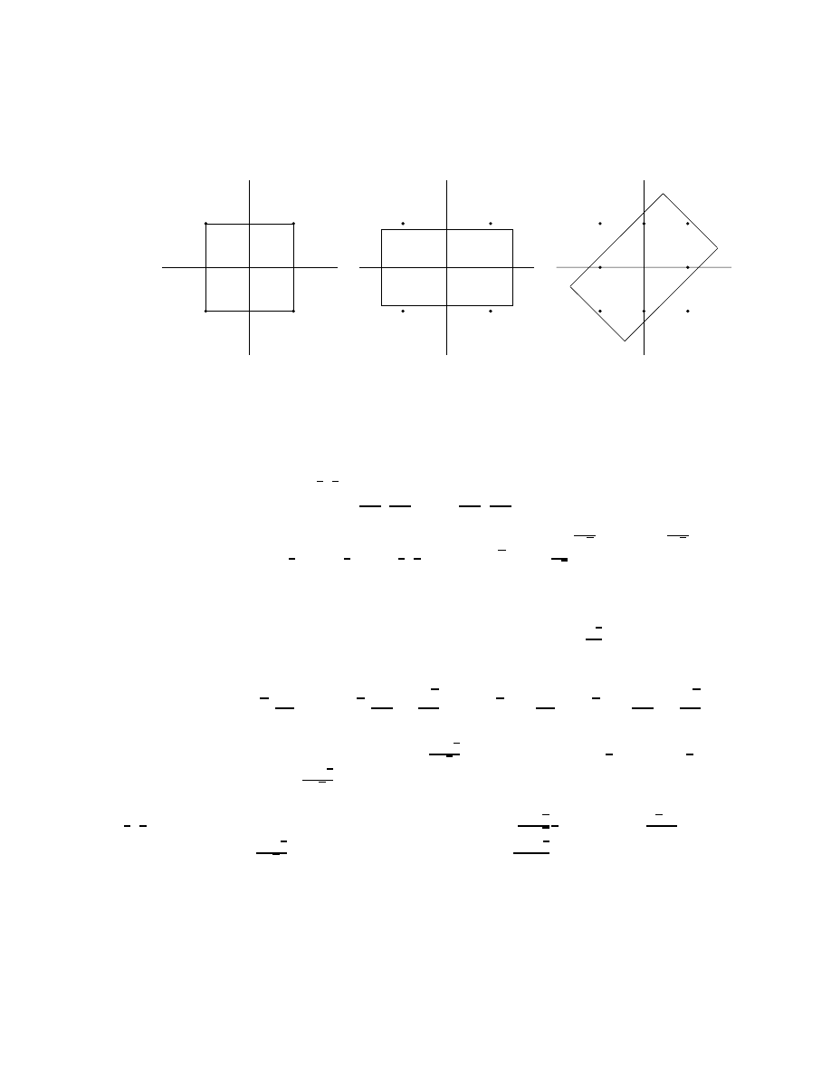
Let us take Ω = [
−
1
2
,
1
2
)
2
, so that Ω
◦
is symmetric with respect to the origin, consistent with
our analysis of longer filters in Section 2.2; this clearly satisfies the first requirement. Then
α
−1
Ω is the rectangle [
−
α
−1
L
2
,
α
−1
L
2
)
× [−
α
−1
H
2
,
α
−1
H
2
). The matrix H
−1
0
rotates this by 45
◦
, to a
tilted rectangle bounded by y = x
±
1
√
2
α
−1
H
, y =
−x ±
1
√
2
α
−1
L
(see Figure 3). In order to satisfy
the second requirement, this tilted rectangle can have area at most 1, or α
H
α
L
>
1. Can we
choose α
L
, α
H
so as to achieve the extremum α
H
α
L
= 1? In that case H
−1
0
α
−1
Ω must be a
fundamental region itself. For this, it is sufficient that (0,
1
2
), (
1
2
, 0) and (
1
2
,
1
2
)
∈ H
−1
0
α
−1
Ω, or
1
2
6
1
√
2
α
−1
H
, 1
6
1
√
2
α
−1
L
. This leads to the choices α
H
=
√
2, α
L
=
1
√
2
, which do indeed satisfy
α
L
α
H
= 1. For the Haar case, we can therefore find a non-uniform expansion matrix corre-
sponding with a global expansion factor of 1 (i.e., no net expansion factor), a significant gain
over the uniform case. Note that the total transform αH
0
is then given by
x
y
!
→
x+y
2
x
− y
!
,
(2.17)
a (non-orthonormal) form of the Haar transform often used in practice, and one which has been
known to lead to a map of integers to integers, called the S-transform [39]. We shall come back
to this in Section 3.1.
After this warm-up, let us consider longer filters. We can re-use much of what was done in
the previous section. The factorization (2.12) becomes now
H
−1
α
−1
= A
..
.
..
.
..
.
· · · 0 0 1 0
· · · 0 0 0 0
C
1
. . . C
N −2
0
0
0
0
· · ·
0
1
0
0
· · ·
..
.
..
.
..
.
B
α
−1
,
which suggests that we seek Ω = αB
−1
R
a,b
so that (
αH)
−1
(Ω
× . . . × Ω) ⊂ (AR
c,d
× . . . × AR
c,d
)
where R
◦
c,d
T
1
2
A
−1
Z
2
=
{0}. Let us check what this leads to in a few examples. We first take
the 4-tap orthonormal filter. In that case, there are no C-matrices to worry about, and we have
17
b
c
a
(-1/2,-1/2)
(1/2,-1/2)
(-1/2,1/2)
(1/2,1/2)
Figure 3.
a. The square Ω =
−
1
2
,
1
2
2
b. Applying α
−1
leads to
h
−
α
−1
L
2
,
α
−1
L
2
×
h
−
α
−1
H
2
,
α
−1
H
2
c. Applying next H
−1
0
leads to the rectangle given by
|y − x|
6
α
−1
H
√
2
,
|y + x|
6
α
−1
L
√
2
.
This contains (
1
2
, 0), (0,
1
2
) and (
1
2
,
1
2
) if α
H
>
√
2, α
L
>
1
√
2
.
c = a, d = b. The matrix A (= V
t
in the notations of the first part of Section 2.2) is still the
same rotation, so we still choose R
c,d
to be the square given by c = d =
√
3
4
. Because α
L
6= α
H
,
the set αB
−1
R
a,b
will no longer be a square; it is the parallelogram
Ω =
{(x, y); |(1 +
√
3)
x
α
L
+ (1
−
√
3)
y
α
H
|
6
√
6
2
and
|(
√
3
− 1)
x
α
L
+ (
√
3 + 1)
y
α
H
|
6
√
6
2
} .
If we assume α
L
6
α
H
, then the condition α
L
>
1+
√
3
√
6
already ensures that (
1
2
, 0) and (0,
1
2
)
∈ Ω.
If we pick the minimal α
L
=
1+
√
3
√
6
' 1.1, does there exist a solution for α
H
and how large does it
need to be? With the notation α
H
= α
L
· δ, with δ
>
1, the parallelogram Ω contains the point
(
1
2
,
1
2
) (and therefore also a fundamental region for Z
2
) if
1 +
1−
√
3
1+
√
3
1
δ
6
1, or δ
>
√
3+1
2
, leading
to the solution α
H
=
2+
√
3
√
6
' 1.6. The product α
L
α
H
is then
5+3
√
3
6
' 1.7, an improvement over
α
2
= 2 in the uniform expansion case, although it is not as spectacular as in the Haar case.
Our next example is the 6-tap orthonormal filter also considered in Section 2.2. We keep
again the same R
c,d
as before, with c = d
' .5296. The square R
a,b
is also not changed, with
a = b
' .3425. It then remains to determine α
L
, α
H
(minimizing either α
L
or α
L
α
H
) so that
18

αB
−1
R
a,b
contains a fundamental region. We have
αB
−1
R
a,b
=
{(x, y);
λ
x
α
L
+
y
α
H
6
a(λ
2
+ 1) ,
x
α
L
− λ
y
α
H
6
b(λ
2
+ 1)
} .
This parallelogram contains (
1
2
, 0), (0,
1
2
) and (
−
1
2
,
1
2
), and therefore a fundamental region for Z
2
,
if α
L
=
1
2a(λ
2
+1)
' 1.4437, α
H
=
1
2a(1−|λ|)(1+λ
2
)
' 1.6147. Again the product α
L
α
H
' 2.3310 is
smaller than the corresponding (1.5965)
2
' 2.5490 in the uniform expansion case, but the gain
is not as dramatic as in the Haar case: we still have α
L
α
H
> 1; worse, even α
L
is still larger
than
√
2.
Finally, let us revisit the biorthogonal example at the end of Section 2.2. Again, the values
of c, d, and a, b can be carried over, and we consider
αB
−1
R
a,b
=
(x, y);
y
α
H
6
1
3
,
x
α
L
+
y
4α
H
6
5
12
.
This contains (
1
2
, 0), (0,
1
2
) and (
−
1
2
,
1
2
) if α
L
=
6
5
, α
H
=
3
2
, a gain over uniform expansion, but
still a rather large price to pay, when compared to the Haar case (where we obtained α
L
< 1!).
In the next section, a different approach is explained, which goes beyond the reduction to
2D used so far, and which enables us to reduce any wavelet filtering to a map from integers
to integers without global expansion. In fact, this amounts to constructing appropriate sets
Γ
n
without using products of 2D regions by using a different representation of the filtering
operations.
3. The lifting scheme and integer to integer transforms
3.1. The S transform. We return again to the Haar transform, which we write in its unnor-
malized version (2.17) involving simply pairwise averages and differences:
s
1,l
=
s
0,2l
+ s
0,2l+1
2
d
1,l
=
s
0,2l+1
− s
0,2l
.
(3.1)
Its inverse is given by
s
0,2l
=
s
1,l
+ d
1,l
/2
s
0,2l+1
=
s
1,l
− d
1,l
/2 .
(3.2)
Because of the division by two, this is not an integer transform. Obviously we can build an
integer version by simply omitting the division by two in the formula for s
1,l
and calculating
the sum instead of the average; this is effectively what was proposed in Section 2.1. But a
more efficient construction, known as the S transform (Sequential), is possible [24, 16]. Several
19

definitions of the S transform exist, differing only in implementation details. We consider the
following case:
s
1,l
=
b(s
0,2l
+ s
0,2l+1
)/2
c
d
1,l
=
s
0,2l+1
− s
0,2l
.
(3.3)
At first sight, the rounding-off in this definition of s
1,l
seems to discard some information.
However, the sum and the difference of two integers are either both even or both odd. We can
thus safely omit the last bit of the sum, since it is equal to the last bit of the difference. The
S-transform thus is invertible and the inverse is given by
s
0,2l
=
s
1,l
− bd
1,l
/2
c
s
0,2l+1
=
s
1,l
+
b(d
1,l
+ 1)/2
c .
(3.4)
As long as the S-transform is viewed as a way to exploit that the sum and difference of two
integers have the same parity, it is not clear how to generalize this approach to other wavelet
filters. A different way of writing the Haar transform, using “lifting” steps
1
, leads to a natural
generalization. Lifting is a flexible technique that has been used in several different settings,
for an easy construction and implementation of “traditional” wavelets [32], and of “second
generation” wavelets [33], such as spherical wavelets [26]. Lifting is also closely related to several
other techniques [13, 22, 37, 34, 20, 4, 15, 7, 3, 19, 28]. Rather than giving the general structure
of lifting at this point, we show how to rewrite the Haar and S transforms using lifting.
We rewrite (3.1) in two steps which need to be executed sequentially. First compute the
difference and then use the difference in the second step to compute the average:
d
1,l
=
s
0,2l+1
− s
0,2l
s
1,l
=
s
0,2l
+ d
1,l
/2 .
(3.5)
This is the same as the Haar transform (3.1) because s
0,2l
+ d
1,l
/2 = s
0,2l
+ s
0,2l+1
/2
− s
0,2l
/2 =
s
0,2l
/2 + s
0,2l+1
/2 . It is now immediately clear how to compute the inverse transform again
in two sequential steps. First recover the even sample from the average and difference, and
later recover the odd sample using the even and the difference. The equations can be found by
reversing the order and changing the signs of the forward transform:
s
0,2l
=
s
1,l
− d
1,l
/2
s
0,2l+1
=
d
1,l
+ s
0,2l
.
1
The name “lifting” was coined in [32], where it was developed to painlessly increase (“lift”) the number of
vanishing moments of a wavelet.
20

As long as the transform is written using lifting, the inverse transform can be found immediately.
We will show below how this works for longer filters or even for non-linear transforms.
We can change (3.5) into an integer transform by truncating the division in the second step:
d
1,l
=
s
0,2l+1
− s
0,2l
s
1,l
=
s
0,2l
+
bd
1,l
/2
c .
This is the same as the S transform (3.3) because s
0,2l
+
bd
1,l
/2
c = s
0,2l
+
bs
0,2l+1
/2
− s
0,2l
/2
c =
bs
0,2l
/2 + s
0,2l+1
/2
c .
Even though the transform now is non-linear, lifting allows us to immediately find the inverse.
Again the equations follow from reversing the order and changing the signs of the forward
transform:
s
0,2l
=
s
1,l
− bd
1,l
/2
c
s
0,2l+1
=
d
1,l
+ s
0,2l
.
Substituting and using that d
− bd/2c = b(d + 1)/2c, we see that this is the same as the inverse
S transform (3.4).
This example shows that lifting allows us to obtain an integer transform using simply trun-
cation and without losing invertibility.
3.2. Beyond the S transform. Two generalizations of the S transform have been proposed:
the TS transform [39] and the S+P transform [25]. The idea underlying both is the same: add a
third stage in which a prediction of the difference is computed based on the average values; the
new high pass coefficient is now the difference of this prediction and the actual difference. This
can be thought of as another lifting step and therefore immediately results in invertible integer
wavelet transforms.
We first consider the TS transform. The idea here is to build an integer version of the
(3, 1) biorthogonal wavelet transform of Cohen-Daubechies-Feauveau [6]. We present it here
immediately using sequential lifting steps. The original, non-truncated transform goes in three
steps. The first two are simply Haar using a preliminary high pass coefficient d
(1)
1,l
. In the last
step the real high pass coefficient d
1,l
is found as d
(1)
1,l
minus its prediction:
d
(1)
1,l
=
s
0,2l+1
− s
0,2l
s
1,l
=
s
0,2l
+ d
(1)
1,l
/2
d
1,l
=
d
(1)
1,l
+ s
1,l−1
/4
− s
1,l+1
/4 .
(3.6)
21

The prediction for the difference thus is s
1,l+1
/4
− s
1,l
/4. The coefficients of the prediction are
chosen so that in case the original sequence was a second degree polynomial in l, then the new
wavelet coefficient d
1,l
is exactly zero. This assures that the dual wavelet has three vanishing
moments. This prediction idea also connects to average-interpolation as introduced by Donoho
in [12]. Substituting we see that the high pass filter is
{1/8, 1/8, −1, 1, −1/8, −1/8} while the
low pass filter is
{1/2, 1/2}, and we thus indeed calculate the (3,1) transform from [6]. Here the
numbers 3 and 1 stand respectively for the number of vanishing moments of the analyzing and
synthesizing high pass filter. We shall follow this convention throughout.
The integer version or TS-transform now can be obtained by truncating the non-integers
coming from the divisions in the last two steps:
d
(1)
1,l
=
s
0,2l+1
− s
0,2l
s
1,l
=
s
0,2l
+
bd
(1)
1,l
/2
c
d
1,l
=
d
(1)
1,l
+
bs
1,l−1
/4
− s
1,l+1
/4 + 1/2
c .
(3.7)
In the last step we add a term 1/2 before truncating to avoid bias; in the second step this is not
needed because the division is only by two. As the transform is already decomposed into lifting
steps, the inverse again can be found immediately by reversing the equations and flipping the
signs:
d
(1)
1,l
=
d
1,l
− bs
1,l−1
/4
− s
1,l+1
/4 + 1/2
c
s
0,2l
=
s
1,l
− bd
(1)
1,l
/2
c
s
0,2l+1
=
d
(1)
1,l
+ s
0,2l
.
(3.8)
The S+P transform (S transform + Prediction) goes even further. Here the predictor for d
(1)
1,l
does not only involve s
1,k
values but also a previously calculated d
(1)
1,l+1
value. The general form
of the transform is
d
(1)
1,l
=
s
0,2l+1
− s
0,2l
s
1,l
=
s
0,2l
+
bd
(1)
1,l
/2
c
d
1,l
=
d
(1)
1,l
+
bα
−1
(s
1,l−2
− s
1,l−1
) + α
0
(s
1,l−1
− s
1,l
) + α
1
(s
1,l
− s
1,l+1
)
− β
1
d
(1)
1,l+1
c .(3.9)
Note that the TS-transform is a special case, namely when α
−1
= β
1
= 0 and α
0
= α
1
= 1/4.
Said and Pearlman examine several choices for (α
w
, β
1
) and in the case of natural images suggest
α
−1
= 0, α
0
= 2/8, α
1
= 3/8 and β
1
=
−2/8. It is interesting to note that, even though this
was not their motivation, this choice without truncation yields a high pass analyzing filter with
2 vanishing moments.
22
3.3. The lifting scheme. We mentioned that the S, TS, and S+P transform can all be seen
as special cases of the lifting scheme. In this section, we describe the lifting scheme in general
[32, 33]. There are two ways of looking at lifting: either from the basis function point of view
or from the transform point of view. We consider the transform point of view.
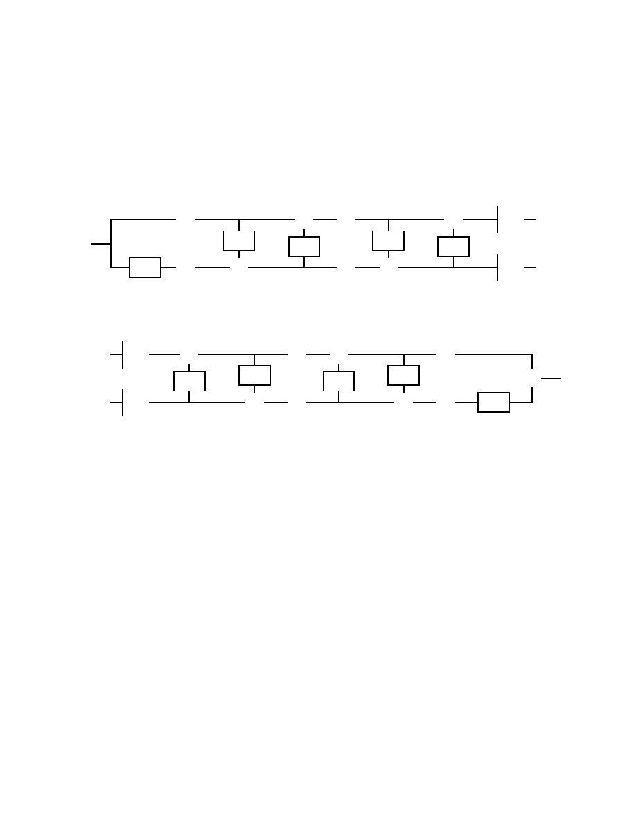
-
-
-
z
-
↓ 2
↓ 2
p
(1)
-
+
−
?
?
u
(1)
-
−
+
-
-
6
6
· · ·
· · ·
p
(M)
-
−
+
?
?
u
(M)
-
−
+
6
6
H
H
H
K
-
H
H
H
1/K
-
BP
LP
Figure 4.
The forward wavelet transform using lifting: First the Lazy wavelet,
then alternating dual lifting and lifting steps, and finally a scaling.
BP
LP
H
H
H
1/K
H
H
H
K
u
(M)
-
+
6
6
p
(M)
-
+
?
?
· · ·
· · ·
u
(1)
-
+
6
6
p
(1)
-
+
?
?
↑ 2
↑ 2
-
z
−1
6
?
+
-
Figure 5.
The inverse wavelet transform using lifting: First a scaling, then
alternating lifting and dual lifting steps, and finally the inverse Lazy transform.
The inverse transform can immediately be derived from the forward by running
the scheme backwards and flipping the signs.
Computing the wavelet transform using lifting steps consists of several stages. The idea is to
first compute a trivial wavelet transform (the Lazy wavelet or polyphase transform) and then
improve its properties using alternating lifting and dual lifting steps, see Figure 4. The Lazy
wavelet only splits the signal into its even and odd indexed samples:
s
(0)
1,l
=
s
1,2l
d
(0)
1,l
=
s
1,2l+1
.
A dual lifting step consists of applying a filter to the even samples and subtracting the result
from the odd ones:
d
(i)
1,l
= d
(i−1)
1,l
−
X
k
p
(i)
k
s
(i−1)
1,l−k
.
23

A lifting step does the opposite: applying a filter to the odd samples and subtracting the result
from the even samples:
s
(i)
1,l
= s
(i−1)
1,l
−
X
k
u
(i)
k
d
(i)
1,l−k
.
Eventually, after, say M pairs of dual and primal lifting steps, the even samples will become the
low pass coefficients while the odd samples become the high pass coefficients, up to a scaling
factor K:
s
1,l
= s
(M)
1,l
/K and d
1,l
= K d
(M)
1,l
.
As always, we can find the inverse transform by reversing the operations and flipping the
signs, see Figure 5. We thus first compute
s
(M)
1,l
= K s
1,l
and d
(M)
1,l
= d
1,l
/K .
Then undo the M alternating lifting steps and dual lifting steps:
s
(i−1)
1,l
= s
(i)
1,l
+
X
k
u
(i)
k
d
(i)
1,l−k
,
and
d
(i−1)
1,l
= d
(i)
1,l
+
X
k
p
(i)
k
s
(i−1)
1,l−k
.
Finally retrieve the even and odd samples as
s
1,2l
= s
(0)
1,l
s
1,2l+1
= d
(0)
1,l
.
The following theorem holds:
Theorem 3.1. Every wavelet or subband transform with finite filters can be obtained as the
Lazy wavelet followed by a finite number of primal and dual lifting steps and a scaling.
This theorem follows from a factorization well known to both electrical engineers (in linear
system theory) as well as algebraists (in algebraic K-theory); [9] gives a self-contained proof
as well as many examples coming from wavelet filter banks.. The proof is constructive; for a
given wavelet transform, the filters used in the lifting steps can be found using the Euclidean
algorithm. The number of lifting steps is bounded by the length of the original filters. It is also
shown in [9] how, with at most 3 extra lifting steps, K can always be set to 1.
It is important to point out that the lifting factorization is not unique. For a given wavelet
transform, one can often find many quite different factorization. Depending on the application
24

one then chooses the factorization with the smallest M , or the one with K closest to one, or the
one which preserves symmetry.
3.4. Lifting and integer wavelet transforms. Since we can write every wavelet transform
using lifting, it follows that we can build an integer version of every wavelet transform. Like
in the examples, one can, in each lifting step round-off the result of the filter right before the
adding or subtracting. An integer dual lifting step thus becomes:
d
(i)
1,l
= d
(i−1)
1,l
− b
X
k
p
(i)
k
s
(i−1)
1,l−k
+ 1/2
c ,
while an integer primal lifting step is given by
s
(i)
1,l
= s
(i−1)
1,l
− b
X
k
u
(i)
k
d
(i)
1,l−k
+ 1/2
c .
This obviously results in an integer to integer transform. Because it is written using lifting steps,
it is invertible and the inverse again immediately follows by flipping the signs and reversing the
operations.
The issue of the scaling factor K remains. Two solutions are possible:
1. Omit the scaling factor K, and keeping in mind that one actually calculates the low pass
times K and the band pass divided by K. This approach is similar to the non uniform
expansion factor of Section 2.3, with the difference that now the product of the factor for
the low pass (K) and the factor for the high pass (1/K) is always one. In this case it is
preferable to let K be as close to 1 as possible. This can be done using the non-uniqueness
of the lifting factorization [9].
2. With three extra lifting steps K can be made equal to one. One can then build the integer
version of those extra lifting steps. This comes down to shifting one coefficient b bits to
the left and the other b bits to the right. The b bits that get lost in the shift to the right
end up in the b locations freed up by the shift to the left.
This leads to the following pseudo-code implementation of an invertible integer wavelet trans-
form using lifting:
s
(0)
1,l
:= s
0,2l
d
(0)
1,l
:= s
0,2l+1
for i = 1:(1):M
∀l : d
(i)
1,l
:= d
(i−1)
1,l
− b
P
k
p
(i)
k
s
(i−1)
1,l−k
+ 1/2
c
∀l : s
(i)
1,l
:= s
(i−1)
1,l
− b
P
k
u
(i)
k
d
(i)
1,l−k
+ 1/2
c
25

end
The inverse transform is given by:
for i = M:(-1):1
∀l : s
(i−1)
1,l
:= s
(i)
1,l
+
b
P
k
u
(i)
k
d
(i)
1,l−k
+ 1/2
c
∀l : d
(i−1)
1,l
:= d
(i)
1,l
+
b
P
k
p
(i)
k
s
(i−1)
1,l−k
+ 1/2
c
end
s
0,2l+1
:= d
(0)
1,l
s
0,2l
:= s
(0)
1,l
3.5. Links with the approach in Section 2. There are two ways in which the scheme from
Section 3.4 can be linked to the approach in Section 2. First of all, by writing the filter bank as
a succession of lifting steps, we have in fact reduced everything to a situation similar to LTF:
every simple lifting step consists in “correcting” one entry (d
(i)
1,l
or s
(i)
1,l
) by adding to it a linear
combination of previously encountered entries. In LTF, the entry to be corrected is nudged away
from its integer value by subtracting from it the fractional part of what will be added by the
filter, but the filtering itself is then untouched. We choose to keep the integer value of the entry
to be corrected, but to change the filter step, adding only the integer part of the correction.
This amounts of course to the same thing.
A second link is the realization that we have in fact constructed in Section 3.4 particular
sets in R
2L
analogous to the H
−1
Γ + n considered in Section 2. To see this, note that if the
lifting scheme, with the truncation to integers of the “lifted” part (but not the first term) at
every step, is applied to real entries instead of integers, the final outcome will also consist of real
numbers (s
(M)
1,l
or d
(M)
1,l
). For each choice n = (n
s,l
, n
d,l
)
l=1,...L
∈ Z
2L
we can define the region
Σ
n
for which
bs
(M)
1,l
c = n
s,l
,
bd
(M)
1,l
c = n
d,l
. These regions correspond to the H
−1
Γ + n that we
considered in Section 2.
The regions Σ
n
are quite complex, however, and do not have the structure proposed in
Section 2.2 or 2.3. Applied to the same data, they will also give different results. The different
Σ
n
need not be even translates of Σ
0
. To illustrate this, let us look at the filters for the integer
TS transform as in (3.7). For simplicity, we take wraparound at the edges. Then the 2L entries
s
0,0
, . . . , s
0,2L−1
get transformed into s
1,l
, d
1,l
with l = 0, . . . , L
− 1, as given by (3.7), with the
boundary cases given by
d
1,0
= d
(1)
1,0
+
b1/4 (s
1,L−1
− s
1,1
) + 1/2
c
d
1,L−1
= d
(1)
1,2L−2
+
b1/4 (s
1,L−2
− s
1,0
) + 1/2
c .
26

The region Σ
0
is now
Σ
0
=
{(s
0,0
, . . . , s
0,2L−1
) ; 0
6
s
1,l
< 1, 0
6
d
1,l
< 1, l = 0, . . . , L
− 1} .
Since
b1/4(a − b) + 1/2c = 0 if bac = bbc = 0, we find that Σ
0
is exactly
Σ
0
=
{(s
0,0
, . . . , s
0,2L−1
) ; 0
6
s
0,2l+1
− s
0,2l
< 1, 0
6
s
0,2l+1
+ s
0,2l
< 2, l = 0, . . . , L
− 1},
or a product of L tiles identical (up to a shift) to those we found for the non-uniform expansion
Haar case in Section 2.3. Define now 2
k
= (s
1,l
, d
1,l
)
l=1,... ,L−1
, with d
1,l
= 0 for all l, s
1,l
= 2 δ
l,k
.
Then
Σ
2
k
=
{(s
0,0
, . . . , s
0,2L−1
) ; 2
6
s
1,k
< 3
0
6
s
1,l
< 1, l = 0, . . . , L
− 1, l 6= k,
0
6
d
1,l
< 1, l = 0, . . . , L
− 1} .
One easily checks that the integer in Σ
2
k
is m
k
= (0, . . . , 0, 2, 2, 1, 0, . . . , 0), i.e., s
0,2k
=
s
0,2k+1
= 2, s
0,2k+2
= 1, all other s
0,l
= 0. Take now s
0
= (0, . . . , 0, 2.9, 2.9, 1, 0, . . . , 0)
∈
Σ
0
+ m
k
. Then d
(1)
1,l
=
−δ
l,k+1
, s
1,l
= 2.9 δ
l,k
, d
1,l
=
−δ
l,k−1
, so that s
0
6∈ Σ
2
k
.
Note that in this particular case Σ
0
happens to be a fundamental region for Z
2L
; in general
(and in particular, in some of the more complex examples that we implemented) even this is not
necessarily true. In most cases, especially when even more truncation steps are considered, Σ
0
can also not be written as a product of two-dimensional regions.
4. Examples
4.1. Interpolating transforms. The first group of examples are instances of a family of sym-
metric, biorthogonal wavelet transforms built from the interpolating Deslauriers-Dubuc scaling
functions [32]. We present examples of the form (N, ˜
N ) where N is the number of vanishing
moments of the analyzing high pass filter, while ˜
N is the number of vanishing moments of the
synthesizing high pass filter. Using this notation the S-transform (3.3) can be referred to as a
(1, 1) transform. For all the interpolating examples we take K = 1.
• (2,2) interpolating transform
d
1,l
= s
0,2l+1
− b1/2 (s
0,2l
+ s
0,2l+2
) + 1/2
c
s
1,l
= s
0,2l
+
b1/4 (d
1,l−1
+ d
1,l
) + 1/2
c .
(4.1)
Note that, up to a shift where s
1,l
here corresponds to s
1,l+1
before, this is exactly the
filter pair given in (2.16).
27

• (4,2) interpolating transform
d
1,l
= s
0,2l+1
− b9/16 (s
0,2l
+ s
0,2l+2
)
− 1/16 (s
0,2l−2
+ s
0,2l+4
) + 1/2
c
s
1,l
= s
0,2l
+
b1/4 (d
1,l−1
+ d
1,l
) + 1/2
c .
(4.2)
• (2,4) interpolating transform
d
1,l
= s
0,2l+1
− b1/2 (s
0,2l
+ s
0,2l+2
) + 1/2
c
s
1,l
= s
0,2l
+
b19/64 (d
1,l−1
+ d
1,l
)
− 3/64 (d
1,l−2
+ d
1,l+1
) + 1/2
c .
(4.3)
• (6,2) interpolating transform
d
1,l
= s
0,2l+1
− b75/128 (s
0,2l
+ s
0,2l+2
)
− 25/256 (s
0,2l−2
+ s
0,2l+4
)
+ 3/256 (s
0,2l−4
+ s
0,2l+6
) + 1/2
c
s
1,l
= s
0,2l
+
b1/4 (d
1,l−1
+ d
1,l
) + 1/2
c .
(4.4)
• (4,4) interpolating transform
d
1,l
= s
0,2l+1
− b9/16 (s
0,2l
+ s
0,2l+2
)
− 1/16 (s
0,2l−2
+ s
0,2l+4
) + 1/2
c
s
1,l
= s
0,2l
+
b9/32 (d
1,l−1
+ d
1,l
)
− 1/32 (d
1,l−2
+ d
1,l+1
) + 1/2
c .
(4.5)
4.2. (2+2,2) transform. Inspired by the S+P transform, we use one extra lifting step to build
the earlier (2, 2) into a transform with 4 vanishing moments of the high pass analyzing filter.
The resulting transform is different from the earlier (4, 2) transform and therefore is called the
(2 + 2, 2) transform. The idea is to first compute a (2, 2) yielding low pass samples s
1,l
and
preliminary detail or high pass samples d
(1)
1,l
, and then use the s
1,l
combined with d
1,l+n
(n > 0)
to compute d
0
1,l
as a prediction for d
(1)
1,l
. The final detail sample then is d
(1)
1,l
− d
0
1,l
. We suggest a
scheme of the form:
d
(1)
1,l
= s
0,2l+1
− b1/2(s
0,2l
+ s
0,2l+2
) + 1/2
c
s
1,l
= s
0,2l
+
b1/4(d
(1)
1,l−1
+ d
(1)
1,l
) + 1/2
c
d
1,l
= d
(1)
1,l
− bα (−1/2 s
1,l−1
+ s
1,l
− 1/2 s
1,l+1
)
+ β (
−1/2 s
1,l
+ s
1,l+1
− 1/2 s
1,l+2
) + γ d
(1)
1,l+1
+ 1/2
c .
(4.6)
Without truncation, we want the scheme to have 4 vanishing moments.
This leads to the
following conditions:
8 β + 3 γ = 1
4 α + 4 β + γ = 1 .
28

Special cases are: (1) α = 1/6, β = 0, γ = 1/3, (2) α = 1/8, β = 1/8, γ = 0, and (3) α = 1/4, β =
−1/4, γ = 1. In our experiments we found that (2) works considerably better than (1) and (3),
and this is the case we use when we refer to (2 + 2, 2) in Section 5.
4.3. D4 orthogonal transform. The transform follows from the lifting factorization in [9].
d
(1)
l
= s
0,2l+1
− b
√
3 s
0,2l
+ 1/2
c
s
1,l
= s
0,2l
+
b
√
3/4 d
(1)
1,l
+ (
√
3
− 2)/4 d
(1)
1,l−1
+ 1/2
c
d
1,l
= d
(1)
1,l
+ s
1,l+1
.
Here K = (
√
3 + 1)/
√
2
≈ 1.577.
4.4. (9
− 7) symmetric biorthogonal transform. We consider the popular (9 − 7) filter
pair. The analysis low pass filter has 9 coefficients, while the analysis high pass filter has 7
coefficients. Both analysis and synthesis high pass filters have 4 vanishing moments [8]. The
integer transform again follows from the lifting factorization in [9].
d
(1)
1,l
= s
0,2l+1
+
bα (s
1,2l
+ s
1,2l+2
) + 1/2
c
s
(1)
1,l
= s
0,2l
+
bβ (d
(1)
1,l
+ d
(1)
1,l−1
) + 1/2
c
d
1,l
= d
(1)
1,l
+
bγ (s
(1)
1,l
+ s
(1)
1,l+1
) + 1/2
c
s
1,l
= s
(1)
1,l
+
bδ (d
1,l
+ d
1,l−1
) + 1/2
c .
The constants are given by
α
≈ −1.586134342
β
≈ −0.05298011854
γ
≈ 0.8829110762
δ
≈ 0.4435068522
K
≈ 1.149604398 .
5. Evaluation of integer to integer wavelet transforms
In this section, we evaluate the effectiveness of the various wavelet filters described in the
previous section for lossless compression of digital images. For the evaluation, we use selected
images from the set of standard ISO test images [1]. In this set of test images, there are natural
images, computer-generated images, compound images (mixed texts and natural images, e.g.,
“cmpnd1” and “cmpnd2”; “us” is an ultrasound image with text on it) and different types of
29
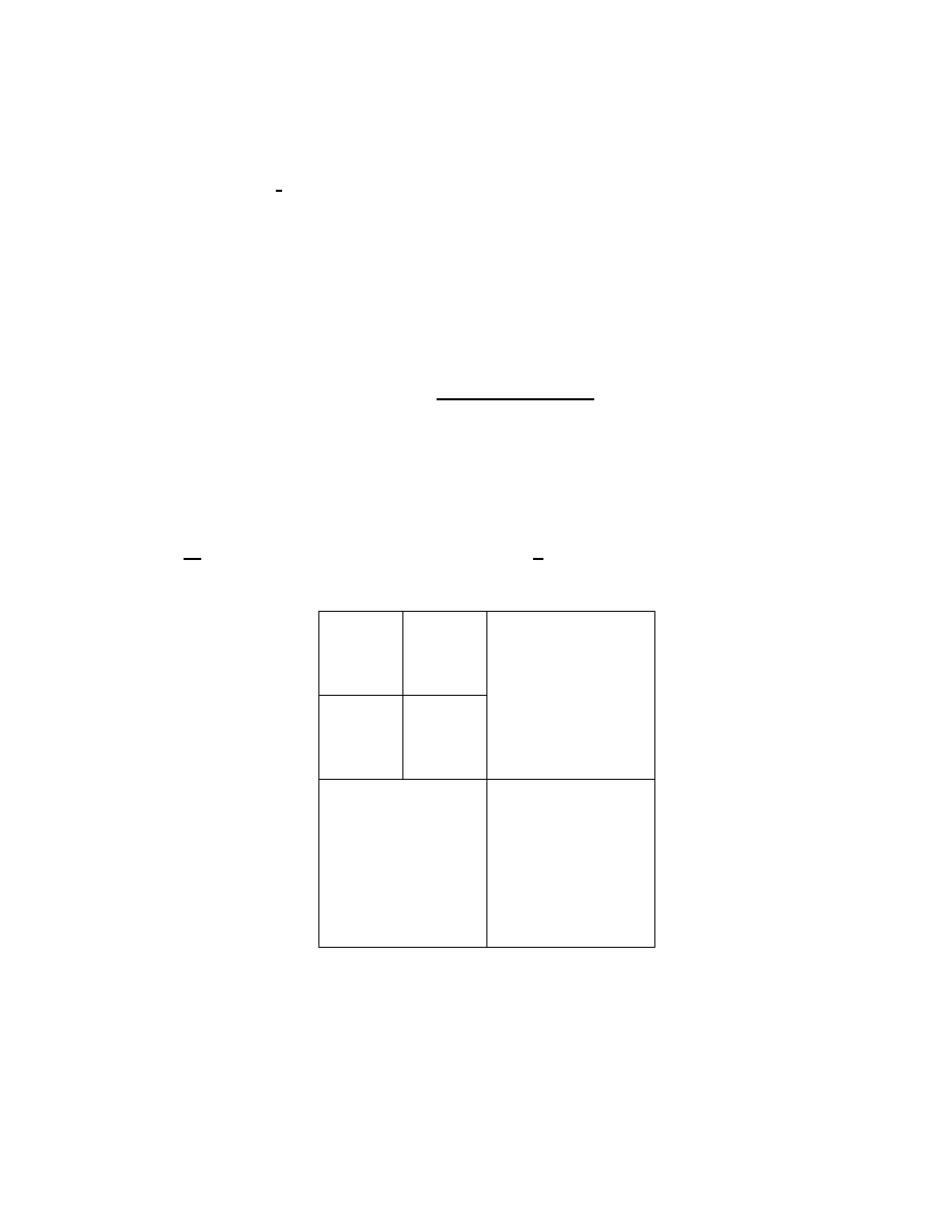
medical images (“x ray”, “cr”, “ct”, and “mri”). Separable two dimensional wavelet transforms
are taken of the images.
The effectiveness for lossless compression is measured using the entropy H(X), given by
H(X) =
−
X
i
P (s
i
) log P (s
i
),
(5.1)
where X is a discrete random variable taking on values s
i
with probability P (s
i
). For an image
X(, ) of size N
× M, we take the probability P (s
i
) to be the normalized count of value s
i
, i.e.,
P (s
i
) =
|(l, m) : X(l, m) = s
i
|
N M
.
(5.2)
We further take into account the fact that the statistics in different quadrants of a wavelet-
transformed image are different, and compute the weighted mean of the entropies in each quad-
rant of the transformed image. For example, in the two-scale decomposition shown in Figure 6,
the weighted entropy (in bits/pixel) is computed as
1
16
(H(C
2
) + H(D
2,v
) + H(D
2,h
) + H(D
2,d
)) +
1
4
(H(D
1,v
) + H(D
1,h
) + H(D
1,d
)) .
D
1,v
D
1,d
D
1,h
D
2,d
D
2,h
D
2,v
C
2
Figure 6.
A two-scale wavelet decomposition.
In the evaluation, we decompose each image into a maximum of five scales, the length and
width permitting. The weighted entropies are tabulated in Table 1.
Several observations can be made:
30

Images
(1,1)
(3,1)
(2,2)
S+P
(4,2)
(2+2,2)
D4
9-7
air2
5.13
4.91
4.82
4.81
4.77
4.76
5.09
4.98
bike
4.36
4.28
4.19
4.18
4.20
4.21
4.37
4.31
cafe
5.69
5.54
5.41
5.42
5.41
5.41
5.63
5.51
cats
3.69
3.53
3.47
3.43
3.42
3.42
3.60
3.47
cmpnd1
2.25
2.84
2.79
2.97
3.31
3.36
3.04
3.45
cmpnd2
2.41
2.96
2.79
3.01
3.28
3.33
3.12
3.42
cr
5.40
5.25
5.20
5.24
5.22
5.22
5.28
5.22
ct
5.54
4.63
4.50
4.30
4.15
4.16
4.96
4.36
faxballs
1.61
1.31
1.08
1.41
1.36
1.17
1.54
1.97
finger
6.24
5.71
5.49
5.48
5.35
5.35
5.85
5.45
gold
4.27
4.10
4.05
4.08
4.04
4.03
4.19
4.14
graphic
3.18
2.82
2.60
2.67
2.56
2.56
3.08
3.00
hotel
4.30
4.18
4.03
4.10
4.06
4.04
4.25
4.18
mri
6.59
6.16
6.02
5.90
5.91
5.91
6.26
5.97
tools
5.84
5.80
5.69
5.73
5.73
5.72
5.88
5.81
us
3.64
3.79
3.69
3.79
3.87
3.85
3.95
4.26
water
2.46
2.45
2.42
2.47
2.45
2.44
2.46
2.50
woman
4.87
4.67
4.57
4.54
4.53
4.54
4.78
4.64
x ray
6.42
6.13
6.06
6.09
6.06
6.06
6.18
6.08
Table 1.
Weighted entropies of transformed images.
1. There is no filter that consistently performs better than all the other filters on all the test
images.
2. Wavelet filters with more analyzing vanishing moments generally perform well with nat-
ural and smooth images and not so with images with a lot of edges and high frequency
components, such as with compound images.
3. On the other hand, a low order filter like (1,1) (S-transform) generally performs the worst,
especially with natural images. It does a poor job in decorrelating the images. However,
it performs significantly better on compound images (e.g., “cmpnd1” and “cmpnd2”) than
other higher order filters.
31

4. Wavelet filters (4,2) and (2+2,2) have similar performances and generally perform better
than other filters evaluated. For images “finger” and “ct”, they perform significantly better
than other filters.
5. The filter (3,1) generally performs worse than filters with comparable number of analyzing
vanishing moments.
6. It is interesting to note that even though the S+P has 2 analyzing vanishing moments, it
performs better than the (3,1) which has 3 and has comparable performances with those
with 4. This suggests that there are other factors besides the number of analyzing vanishing
moments which affect compression efficiency.
7. The (9
− 7), which is most popularly used for lossy compression of images and which has 4
analyzing vanishing moments, generally does not perform as well as the (4,2) and (2+2,2),
which have the same number of analyzing vanishing moments.
We further evaluate the wavelet filters by attaching an entropy coder to compute the actual
bit rate. We use the entropy coder of Said and Pearlman [25]. In each quadrant, the wavelet
coefficients are visited in a scanline order; for each coefficient, a context C
j
is derived based on
the values of its adjacent coefficients which have already been visited and its parent coefficient.
A total of 25 different contexts are used. The statistics of the context model is adaptively
updated as more pixels are visited and the model is reset after each quadrant is visited. An
arithmetic coder is then used to code the coefficients according to their contexts. The resulting
bit rate will be lower bounded by the conditional entropy,
H(X
|C) = −
X
i,j
P (s
i
, c
j
) log P (s
i
|c
j
),
(5.3)
where P (s
i
, c
j
) is the joint probability of value s
i
and context c
j
and P (s
i
|c
j
) is the conditional
probability of value s
i
given context c
j
. The results are tabulated in Table 2. The numbers
are derived from compressed file sizes. Given that H(X
|C) ≤ H(X), conditioning allows us to
achieve actual bit rate lower than the entropy H(X) computed in Table 1.
The relative strength of each filter over the others in actual coding is similar to that computed
using the entropies. As previously observed, wavelet filters (4,2) and (2+2,2) generally outper-
forms other filters for natural and smooth images. Also, filters with more analyzing vanishing
moments perform poorly with compound images. As can be seen from the two tables, numbers
computed from entropies provide a good indication of the actual performance of a wavelet filter.
Alternatively, with a context model in mind, one can compute the conditional entropies for a
better estimate of the actual bit rate.
32

Images
(3,1)
(2,2)
S+P
(4,2)
(2+2,2)
D4
9-7
air2
4.34
4.29
4.28
4.24
4.24
4.60
4.52
bike
3.83
3.78
3.76
3.78
3.79
3.94
3.88
cafe
5.07
4.98
4.98
4.95
4.98
5.17
5.07
cats
2.60
2.56
2.53
2.52
2.52
2.67
2.57
cmpnd1
2.34
2.31
2.38
2.59
2.62
2.40
2.64
cmpnd2
2.46
2.33
2.45
2.58
2.61
2.49
2.64
cr
5.21
5.17
5.22
5.19
5.19
5.25
5.20
ct
3.96
3.92
3.70
3.61
3.65
4.30
3.80
faxballs
1.12
1.02
1.20
1.17
1.07
1.51
1.59
finger
5.73
5.56
5.51
5.41
5.42
5.90
5.50
gold
3.99
3.94
3.99
3.95
3.94
4.11
4.09
graphic
3.05
2.91
2.93
2.87
2.89
3.34
3.29
hotel
3.97
3.90
3.95
3.91
3.90
4.10
4.07
mri
5.99
5.90
5.77
5.80
5.81
6.13
5.89
tools
5.59
5.49
5.53
5.52
5.51
5.65
5.60
water
1.83
1.79
1.85
1.81
1.80
1.85
1.88
woman
4.24
4.17
4.15
4.14
4.15
4.37
4.28
us
3.17
3.13
3.16
3.23
3.22
3.38
3.53
x ray
5.99
5.92
5.94
5.92
5.92
6.05
5.95
Table 2.
Exact bit rate of test images.
We also observe that the use of simple context modeling of the wavelet coefficients as in [25]
cannot provide a significant enough gain in actual coding when the performance of the wavelet
filter is poor in the first place. This points to the importance of using “good” wavelet filters and
necessitates the search for such filters.
The classical approach to lossless compression is decomposed into two steps: spatial decor-
relation and entropy coding of the decorrelated signals. The decorrelating steps have always
been performed in the spatial domains and they involve some form of non adaptive or adaptive
prediction of a pixel values based on previously visited pixels (see [23] and the references therein
for comparisons of state-of-the-art spatial-domain predication techniques). In fact, we can view
wavelet transforms that use two lifting steps such as those built from Deslauriers-Dubuc scaling
functions as decorrelation steps. The high pass coefficients are the decorrelated components.
33

The lifting step computes the difference between a true coefficient and its prediction and has
the following form:
d
j+1,l
= s
j,2l+1
− bf(s
j,2l−2L
· · · , s
j,2l−2
, s
j,2l
, s
j,2l+2
, s
j,2l+4
,
· · · , s
j,2l+2L
)
c.
(5.4)
We are thus predicting a pixel at an odd location 2l + 1 using pixels at even locations from both
sides of 2l + 1. This is in contrast to the spatial domain approach to prediction, which has the
following one-sided form:
d
j
= s
j
− bg(s
j−J
,
· · · , s
j−3
, s
j−2
, s
j−1
)
c.
(5.5)
The price to pay for prediction based on (5.4) is to retain knowledge of the remaining pixels
at the even locations. Similar prediction steps can be performed on these remaining pixels,
but because the distances between adjacent pixels are larger than before, correlations between
adjacent pixels tend to be lower. The dual lifting step in generating the s
j+1,l
smoothes this set
of remaining pixels before the lifting step on the coarser level is performed.
The big advantage of using wavelet transform to represent images is multiresolution represen-
tation, which spatial-domain prediction techniques based on (5.5) cannot offer. Using wavelet
transforms that map integers to integers permits lossless representation of the image pixels and
easily allows the transmission of lower resolution versions first, followed by transmissions of suc-
cessive details. Such a mode of transmission is especially valuable in scenarios where bandwidth
is limited, image sizes are large and lossy compression is not desirable. Examples are transmis-
sion of 2-D and 3-D medical images for tele-medicine applications and transmission of satellite
images down to earth. Each of these images is typically several megabytes in size.
Valuable lessons could also be learned from the recent advances in spatial-domain prediction
techniques [23]. Adaptation of prediction methods is made based on local statistics of the pixels.
In the wavelet transform approach to decorrelating an image, we could also use an adaptive
scheme in deciding the use of wavelet filters on a pixel by pixel basis. As we have seen, there
is not a wavelet filter that performs uniformly better than the others. Thus, the activities in
some small neighborhood should be used in determining the type of filters to use. The use of
adaptive wavelet filters in lossless and multiresolution representation of images warrants further
investigation.
Acknowledgements. Ingrid Daubechies would like to thank NSF (grant DMS-9401785), AFOSR
(grant F49620-95-1-0290), ONR (grant N00014-96-1-0367) as well as Lucent Technologies, Bell
Laboratories for partial support while conducting the research for this paper. I. D. and A.
R. Calderbank would like to thank the Institut des Hautes Etudes Scientifiques in Bures-sur-
Yvette, France, for its hospitality and support in June ’95 when part of this work was done.
34

Wim Sweldens is on leave as Senior Research Assistant of the Belgian Fund of Scientific Re-
search (NFWO). Boon-Lock Yeo thanks the support of the IBM Graduate Fellowship in spring,
AT&T Bell Laboratories in summer, and the Wallace Memorial Fellowship in Engineering from
Princeton University in fall 1995.
Note. After finishing this work, we learned that a construction similar to the one presented in
Section 3 was obtained independently by Dewitte-Cornelis and Chao-Fischer [11, 5].
The Chao-Fischer approach has the extra feature that it uses modular arithmetic to eliminate
all increase in dynamic range; thus if the original image uses 8 bits per pixel, all the wavelet
coefficients uses 8 bits as well. The disadvantage is that large wavelet coefficients can become
small due to the modular arithmetic, and vice versa. In our experiments, this wraparound
disadvantage tends to cancel out the advantage of no bit growth; nevertheless it is useful for
certain implementations.
References
[1] ISO/IEC JTC 1/SC29/WG1. Call for contributions - lossless compression of continuous-tone still pictures.
ISO Working Document ISO/IEC JTC1/SC29/WG1 N41, March 1994.
[2] C. M. Brislawn, J. N. Bradley, R. J. Onyshczak, and T. Hopper. The FBI compression standard for digitized
fingerprint images. In A. G. Tescher, editor, Applications of Digital Image Processing XIX. Proc. SPIE 2847,
1996.
[3] A. A. M. L. Bruekens and A. W. M. van den Enden. New networks for perfect inversion and perfect recon-
struction. IEEE J. Selected Areas Commun., 10(1), 1992.
[4] J. M. Carnicer, W. Dahmen, and J. M. Pe˜
na. Local decompositions of refinable spaces. Appl. Comput.
Harmon. Anal., 3:127–153, 1996.
[5] H. Chao and P. Fisher. An approach of fast integer reversible wavelet transform for image compression.
Preprint.
[6] A. Cohen, I. Daubechies, and J. Feauveau. Bi-orthogonal bases of compactly supported wavelets. Comm.
Pure Appl. Math., 45:485–560, 1992.
[7] W. Dahmen and C. A. Micchelli. Banded matrices with banded inverses II: Locally finite decompositions of
spline spaces. Constr. Approx., 9(2-3):263–281, 1993.
[8] I. Daubechies. Ten Lectures on Wavelets. CBMS-NSF Regional Conf. Series in Appl. Math., Vol. 61. Society
for Industrial and Applied Mathematics, Philadelphia, PA, 1992.
[9] I. Daubechies and W. Sweldens. Factoring wavelet transforms into lifting steps. Technical report, Bell Lab-
oratories, Lucent Technologies, 1996.
[10] R. A. DeVore, B. Jawerth, and B. J. Lucier. Image compression through wavelet transform coding. IEEE
Trans. Inform. Theory, 38(2):719–746, 1992.
[11] S. Dewitte and J. Cornelis. Lossless integer wavelet transform. Technical Report IRIS-TR-0041, Royal Me-
teorological Institute Belgium, 1996.
[12] D. L. Donoho. Smooth wavelet decompositions with blocky coefficient kernels. In [27], pages 259–308.
35

[13] D. L. Donoho. Interpolating wavelet transforms. Preprint, Department of Statistics, Stanford University,
1992.
[14] J. Gros. Binary friendly wavelets. Preprint, Department of Electrical Engineering and Computer Sciences,
UC Berkeley, 1995.
[15] A. Harten. Multiresolution representation of data: A general framework. SIAM J. Numer. Anal., 33(3):1205–
1256, 1996.
[16] V. K. Heer and H-E Reinfelder. A comparison of reversible methods for data compresssion. In Medical Imaging
IV, pages 354–365. Proc. SPIE 1233, 1990.
[17] J. Hong. Discrete Fourier, Hartley and cosine transforms in signal processing. PhD thesis, Columbia Uni-
verisity, Department of Electrical Engineering, 1993.
[18] C. P. Johnston. The lifting scheme and finite-precision-error-free filter banks. In M. Unser, A. Aldroubi,
and A. F. Laine, editors, Wavelet Applications in Signal and Image Processing IV, pages 307–316. Proc.
SPIE 2825, 1996.
[19] T. A. C. M. Kalker and I. Shah. Ladder Structures for multidimensional linear phase perfect reconstruction
filter banks and wavelets. In Proceedings of the SPIE Conference on Visual Communications and Image
Processing (Boston), pages 12–20, 1992.
[20] C. W. Kim, R. Ansari, and A. E. Cetin. A class of linear-phase regular biorthogonal wavelets. In Proc. IEEE
Int. Conference on Acoustics, Speech, Signal Processing, pages 673–676, 1992.
[21] R. Laroia, S. A. Tretter, and N. Farvardin. A simple and effective precoding scheme for noise whitening on
intersymbol interference channels. IEEE Trans. Commun., 41:460–463, 1993.
[22] M. Lounsbery, T. D. DeRose, and J. Warren. Multiresolution surfaces of arbitrary topological type. De-
partment of Computer Science and Engineering 93-10-05, University of Washington, October 1993. Updated
version available as 93-10-05b, January, 1994.
[23] N. Memon, V. Sippy, and X. Wu. A comparison of prediction schemes proposed for a new lossless image
compression standard. In IEEE International Symposium on Circuits and Systems, volume 2, pages 309–312,
May 1995.
[24] M. Rabbini and P. W. Jones. Digital Image Compression Techniques. SPIE Opt. Eng. Press, Bellingham
WA, 1991.
[25] A. Said and W. A. Pearlman. An image multiresolution representation for lossless and lossy image compres-
sion. IEEE Trans. Image Process., 5(9):1303–1310, 1996.
[26] P. Schr¨
oder and W. Sweldens. Spherical wavelets: Efficiently representing functions on the sphere. Computer
Graphics Proceedings, (SIGGRAPH 95), pages 161–172, 1995.
[27] L. L. Schumaker and G. Webb, editors. Recent Advances in Wavelet Analysis. Academic Press, New York,
1993.
[28] I. Shah and T. A. C. M. Kalker. On Ladder Structures and Linear Phase Conditions for Bi-Orthogonal Filter
Banks. In Proceedings of ICASSP-94, volume 3, pages 181–184, 1994.
[29] J. M. Shapiro. Embedded image coding using zerotrees of wavelet coefficients. IEEE Trans. Signal Process.,
41(12):3445–3462, 1993.
[30] G. Strang and T. Nguyen. Wavelets and Filter Banks. Wellesley, Cambridge, 1996.
[31] M. D. Swanson and A. H. Tewfix. A binary wavelet decomposition of binary images. IEEE Trans. Image
Process., 5(12):1637–1650, 1996.
36

[32] W. Sweldens. The lifting scheme: A custom-design construction of biorthogonal wavelets. Appl. Comput.
Harmon. Anal., 3(2):186–200, 1996.
[33] W. Sweldens. The lifting scheme: A construction of second generation wavelets. SIAM J. Math. Anal., to
appear, 1997.
[34] L. M. G. M. Tolhuizen, I. A. Shah, and T. A. C. M. Kalker. On constructing regular filter banks from domain
bounded polynomials. IEEE Trans. Signal Process., 42(2):451–456, 1994.
[35] P. P. Vaidyanathan. Multirate Systems and Filter Banks. Prentice Hall, Englewood Cliffs, NJ, 1992.
[36] P. P. Vaidyanathan and P.-Q. Hoang. Lattice structures for optimal design and robust implementation of
two-band perfect reconstruction QMF banks. IEEE Trans. Acoust. Speech Signal Process., 36:81–94, 1988.
[37] M. Vetterli and C. Herley. Wavelets and filter banks: Theory and design. IEEE Trans. Acoust. Speech Signal
Process., 40(9):2207–2232, 1992.
[38] M. Vetterli and J. Kova˘
cevi´
c. Wavelets and Subband Coding. Prentice Hall, Englewood Cliffs, NJ, 1995.
[39] A. Zandi, M. Boliek, E. L. Schwartz, and M. J. Gormish. CREW lossless/lossy medical image compression.
Technical Report CRC-TR-9526, RICOH California Research Center, 1995.
Appendix
A. Proof of Lemma 2.1
We start by reformulating Lemma 2.1 in a slightly different way, introducing explicit notations
for all the points involved.
Lemma 2.1. Let P be a parallelogram that is a fundamental region for Z
2
, and let A
1
, A
2
, A
3
be three points on the boundary of P such that
• A
0
j
, the mirror image of A
j
with respect to the center of P , is congruent with A
j
modulo
Z
2
(j = 1, 2, or 3)
• no three points among A
1
, A
2
, A
3
, A
0
1
, A
0
2
, A
0
3
are collinear.
Let Ω be the hexagon with vertices A
1
, A
2
, A
3
, A
0
1
, A
0
2
, A
0
3
. Then any closed parallelogram Q that
contains Ω also contains a fundamental region for Z
2
.
(Note that Ω is a strict subset of a fundamental region, and is therefore not a fundamental region
itself.)
Proof. Without loss of generality, we can assume that P is centered around the origin.
Because of the prohibition of collinearity, the six points must be distributed among the four
sides of P , with two points each on two opposite sides, and one point each on the remaining two
sides. If none of the points A
j
, A
0
j
lies on a vertex of P , then we can assume (by renumbering if
necessary) that A
1
, A
2
, and A
3
are three consecutive corners of the hexagon Ω, lying on three
different sides of P ; see Figure 7a. (If one of the A
j
, A
0
j
lies on a vertex, as in Figure 7b, then
the rest of this proof needs to be changed in a straightforward way; we leave this as an exercise
for the reader.)
37
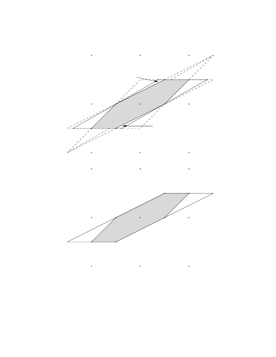
A
1
A
1
A
0
3
C
0
23
A
0
1
A
2
A
2
A
0
2
C
0
12
A
0
2
A
3
A
0
1
23
0
23
0
12
~
12
A
0
3
C
12
12
^
12
A
3
C
23
Figure 7.
a. The parallelogram P (with vertices C
12
, C
23
, C
0
12
, and C
0
23
) and the inscribed
hexagon Ω, with associated triangles
4
12
,
4
23
,
4
0
12
and
4
0
23
. All the
e and b
versions of the triangles are drawn, but only e
4
12
and b
4
12
have been labelled.
b. A special case where some vertices of Ω coincide with vertices of P .
38

Denote by C
12
the vertex of P that separates A
1
from A
2
, and similarly by C
23
the vertex
that separates A
2
from A
3
. We denote their opposites, which separate A
0
1
from A
0
2
, A
0
2
from A
0
3
,
respectively, by C
0
12
and C
0
23
.
The original fundamental region P is the union of the hexagon Ω and four triangles
4
12
(with vertices A
1
, A
2
, C
12
),
4
23
(vertices A
2
, A
3
, C
23
),
4
0
12
(vertices A
0
1
, A
0
2
, C
0
12
), and
4
0
13
(ver-
tices A
0
1
, A
0
3
, C
0
13
). For each of the triangles
4
ij
we define the two triangles b
4
ij
and e
4
ij
by
b
4
ij
=
4
ij
− A
i
+ A
0
i
, e
4
ij
=
4
ij
− A
j
+ A
0
j
; b
4
0
ij
and e
4
0
ij
are defined analogously. Every one of
the four original triangles is congruent modZ
2
with its
b and e versions.
Suppose there exists a parallelogram Q that contains Ω and that does not contain a funda-
mental region for Z
2
. If the parallel lines that bound Q do not touch Ω, we may reduce their
separation until they do. Let R be the resulting reduced parallelogram, bounded by the parallel
lines L, L
0
and M, M
0
, each of which is incident with Ω. Let x be a point in P so that R does
not contain any point congruent to x mod Z
2
. Then x
∈ 4
ij
or
4
0
ij
for some i, j, and there exist
points
bx, ex in the corresponding b
4, e
4 that are congruent to x mod Z
2
. Observe that if L, L
0
are
parallel lines through opposite vertices j, j
0
then exactly two of the points x,
ex, bx lie between L
and L
0
. Similarly for M, M
0
. Hence one of the points x,
ex, bx lies in the parallelogram R bounded
by L, L
0
and M, M
0
, which is a contradiction.
AT&T-Labs Research, Rm. 2C-363, 600 Mountain Avenue, Murray Hill NJ 07974
rc@research.att.com
Program for Applied and Computational Mathematics, Princeton University, Princeton NJ 08544
ingrid@math.princeton.edu
Lucent Technologies, Bell Laboratories, Rm. 2C-376, 600 Mountain Avenue, Murray Hill NJ 07974
wim@bell-labs.com
IBM Thomas J. Watson Research Center, P.O. Box 704, Yorktown Heights, NY 10598
yeo@watson.ibm.com
39
Wyszukiwarka
Podobne podstrony:
Mathematica package for anal and ctl of chaos in nonlin systems [jnl article] (1998) WW
Generalized Power Series in a Non Archimedean Field [jnl article] (1991) WW
Minkowski Metrics [jnl article] (2002) WW
Using Matlab for Solving Differential Equations (jnl article) (1999) WW
Elliptic Curves [jnl article] B Poonen WW
Connectionism Past, Present, and Future [jnl article] J Pollack WW
A Genetic Algorithm Tutorial [jnl article] D Whitley WW
The Birth of Model Theory [jnl article] C Badesa WW
Introduction to Linear Logic T Brauner (1996) WW
Efficient VLSI architectures for the biorthogonal wavelet transform by filter bank and lifting sc
The?ctors that Gave Rise To Japanese Militarism
Juvenile Crime Risk?ctors that Drive Youth to It
Efficient VLSI architectures for the biorthogonal wavelet transform by filter bank and lifting sc
An Introduction to Conformal Field Theory [jnl article] M Gaberdiel (1999) WW
Monte Carlo Sampling of Solutions to Inverse Problems [jnl article] K Mosegaard (1995) WW
Jamie Craig All That You Do To Me
Efficient VLSI architectures for the biorthogonal wavelet transform by filter bank and lifting sc
więcej podobnych podstron