Department of Music and Sound Recording

The Institute of Sound Recording papers

University of Surrey

Year 

An Assessment of the Spatial

Performance of Virtual Home Theatre

Algorithms by Subjective and Objective

Methods

Russell Mason

Francis Rumsey

This paper is posted at Surrey Scholarship Online.

http://epubs.surrey.ac.uk/recording/4

1

An assessment of the spatial performance of virtual home theatre

algorithms by subjective and objective methods

Russell Mason and Francis Rumsey, Institute of Sound Recording,

School of Performing Arts, University of Surrey,

Guildford, Surrey, GU2 5XH, UK

[e-mail]

[e-mail]

Abstract:

A controlled subjective test was carried out to assess selected spatial qualities of three virtual
home theatre processors. The subjective results were used to evaluate a number of objective
measurements based on the interaural cross-correlation coefficient (IACC). A novel
implementation of the IACC was found which appears to correlate well with the subjective
data.

0 Introduction

This paper documents part of the work carried out under the Eureka 1653 MEDUSA
(Multichannel Enhancement of Domestic User Stereo Applications) project. The MEDUSA
project involves collaborative research between the following partners: the British
Broadcasting Corporation, the Institute of Sound Recording at the University of Surrey,
Nokia Research Centre, Genelec Oy, and Bang & Olufsen A/S.

The purpose of the project is to examine the variables of the domestic multichannel sound
system, with and without picture, to carry out the essential optimisation leading to consumer
end products. These products will combine the requirements of multichannel reproduction
together with the less complex modes of reproduction, such as stereo and mono. This involves
linked studies of programme production and perceptual elements, leading to a single
optimised approach to domestic reproduction.

A great deal of the research carried out within the MEDUSA project involves subjective
listening tests. These subjective experiments are both expensive and time consuming to carry
out. As an alternative to this, objective measures that correlate well with certain subjective
parameters would be more accurately repeatable and would save time and money [1].
Therefore, it would be useful if subjective assessments could be replaced or complemented by
objective measurement methods. Currently it may be an impossible task to replace subjective
assessments completely. However, there are measures that are established or under
development which may correlate well with some aspects of spatial perception.

Whilst a great deal of research has been completed into the aspect of localisation in
reproduction systems, ‘spatial impression’ has so far been left behind [2]. Perhaps one reason
for this is the comparative simplicity with which localisation can be evaluated in listening
tests. In contrast, spatial impression is a much more complicated multidimensional subjective
phenomenon. In this case, spatial impression is defined as the auditory perception of the
location, dimensions, and other physical parameters of a sound source and the acoustic
environment in which the source is located.

In some areas, spatial impression has been researched in detail. This includes the perception
of concert hall acoustics. Not all of the measurable or perceivable categories used in concert

2

hall acoustics are relevant to the reproduction of sound in small rooms, but there are definite
parallels. Beranek provides a good overview of this [3].

The research into concert hall acoustics also proposes a number of objective measurements
that help to predict how a listener will perceive the sound of a concert hall. Among these is
the interaural cross-correlation coefficient (IACC), a measurement which was first worked on
in the late 1960s. Work by Schroeder, Gottlob and Siebrasse found that IACC was one of a
number of physical measures that correlated well with listener preferences [4]. Ando
confirmed this and found that it was independent of reverberation time [5].

The IACC has seldom been tested using reproduction systems [6, 7, 8]. There are also
arguments that the IACC is inadequate due to its poor low frequency differentiation [9], and
that the IACC does not work for small rooms [10].

Therefore, an experiment was undertaken to test a reproduction system in a small room using
both subjective and objective measurements. The objective measurements were based on the
IACC and the results were examined to find correlations with subjective spatial attributes.

The reproduction chosen implemented various ‘virtual home theatre’ (VHT) systems as
described in [11]. This type of system aims to reproduce the spatial attributes of the original
multichannel material using only two loudspeakers. This is usually attempted by simulating
head-related transfer function (HRTF) cues with cross-talk cancelling. By using a system in
which some of the loudspeaker signals are already artificially spatialised, the challenge for the
objective measurement is possibly made more difficult.

1 Programme material

In order to quantify attributes of sound reproduction using subjective tests, it is necessary to
conduct controlled listening tests. Within these listening tests an experimental design needs to
limit extraneous variables to an absolute minimum. Because of this, the programme material
needs to contain a wide range of auditory cues, yet be limited enough not to confuse the
listener. Whilst this may in some cases limit the external validity of a test, it is sometimes
necessary in order to obtain sensitive results.

In this case, certain spatial attributes of various virtual home theatre algorithms were judged.
Based on the work of Berg [12], these attributes were limited to those of Apparent Source
Width (ASW), Listener Envelopment (LEV) – both defined in [13], and Depth (perceived
distance of the source from the listener). The simplest programme material available that
would sufficiently excite all three spatial attributes was a single source in a reverberant
environment. To produce a range of auditory cues, a number of acoustic environments and
sound sources were needed.

Therefore, programme material was recorded specifically for this experiment, consisting of a
number of sound sources in a number of acoustic environments. In order to separate the
variables of acoustic environment and sound source, the source was sounded and recorded in
each environment. If this had been done in the conventional manner of recording a
performance in each space, there would have been an additional variable. For a given musical
extract, even with the very best musicians, it would have been impossible to play exactly the
same twice or more. This would have added performance as a confounding variable in
judging the reproduction of the acoustic environments.

Replaying anechoically recorded excerpts through a loudspeaker in each of the acoustic
environments eliminated this variation. This method was necessarily a compromise as there

3

was no longer a real source sounding in each acoustic. The disadvantages of this approach
were due to the artificiality of this ‘virtual source’. This included the directionality of the
source and the physical coupling of the source to the air. Such factors as timbre, attack, decay,
and musicality should have been reproduced effectively by high quality reproduction. This
approach has been used successfully in previous experiments [14, 4].

1.1 Anechoic recordings

The most readily available source of anechoic recordings was the Bang and Olufsen CD that
contains anechoic recordings made for the Archimedes project. The recording of this is well
documented in [15].

In order to present a wide range of auditory cues, the programme material needs to contain a
range of sound sources. This should ideally include examples such as transients, sustains,
both wide-band and narrow-band (tuned) signals, a wide range of frequencies, and a human
voice. There should also be sufficient gaps in the extracts so it is possible to hear the effect of
the acoustics.

The extracts used from the B&O CD were Cello (sustained, tuned, low frequency) and
Trumpet (mixture of transient attacks and sustains, tuned, mid-high frequencies). Two
additional extracts were recorded in the free-field room at BBC Research and Development in
Kingswood Warren, UK. These were snare drum (transient, wide frequency range, separated
hits) and a male speaking voice (a mixture of noise and modulated tonal sounds - a popular
test item).

The recordings were made in mono with a Brüel and Kjær 4006 omnidirectional microphone
connected via a custom pre-amp and phantom power supply to a Tascam DA-30 DAT
recorder using the internal converters. The aim of the recording was to produce a result which
when replayed sounded as natural as possible. In order to do this, the recording was
monitored on a single large loudspeaker and compared with the natural sound from the
source.

It has been found that it is easier and more efficient to judge audio signals that are stationary
and possibly repetitive [2, 16]. Because of this, the snare drum and trumpet excerpts were
made up of a short loop of a bar or so. This loop was repeated for 60 seconds to match the
duration of the other extracts.

The relative reproduction level of each of the sound sources is also important in recreating it
as accurately as possible. Using a Brüel and Kjær SPL meter with a Brüel and Kjær 4145 1-
inch capsule, A-weighted SPL measurements with a fast time constant were made of an
example of each sound source represented. From this, the relative level of each source was
calculated and referenced to a calibration signal of pink noise at 85 dBA at 1 metre from the
loudspeaker. A DAT was compiled of the excerpts adjusted to the correct level. As a final
check, the DAT was replayed at its reference level next to the corresponding source
reproducing a similar phrase.

1.2 Choice of reproduction loudspeaker

After informal listening, it was apparent that the choice of loudspeaker for reproducing the
anechoic recordings was important as it had a significant effect on the perceived result. The
ideal situation would be to reproduce each sound source through a loudspeaker that matches
the source most closely in terms of size, shape, directionality and frequency response.

4

Unfortunately it was not possible to obtain loudspeakers which met all of these criteria for all
the sources. Therefore, it was necessary to compromise on one loudspeaker.

The loudspeakers had to meet the following criteria in order to act effectively as a ‘virtual
source’:

•

Frequency response – fairly flat across a wide frequency range (low cello fundamental to

snare drum transient)

•

Sound power output – capable of emulating a trumpet playing fortissimo (approximately

100dBA at 1 metre)

•

Directionality / polar response – as omnidirectional as possible in order to excite the

response of the room and early reflections as much as possible.

It is recognised that some of the sound sources have a naturally narrow polar response at
certain frequencies. However, to accentuate the difference between the rooms by exciting the
early reflections as much as possible, a more omnidirectional source was needed.

A number of loudspeakers were tested to check whether they met the basic criteria outlined
above. These were: a Rogers LS5/8; a B&W 801; a JBL Control 12 SR; and a Quad
electrostatic.

To select the best of these loudspeakers, all four were listened to in Studio 1 of the PATS
building at the University of Surrey. This was one of the intended acoustic environments. The
loudspeakers were set up one at a time at the central line of the room, 4 metres from the rear
wall. They were each set up to replay at a reference level.

In this listening set-up, the JBL and Quad loudspeakers were found to be unsuitable. The JBL
was too directional due to the horn loaded tweeter. The Quad was not capable of producing a
high SPL, and it had a very limited high frequency response.

Of the remaining two, the Rogers radiated more high frequency content than the B&W. In
terms of perceived spatial impression, the B&W seemed to be a little wider than the Rogers.
In order to quantify the differences in the polar responses of the two loudspeakers, they were
measured in the free-field room at BBC Research and Development using a Maximum Length
Sequence System Analyser (MLSSA) from DRA Laboratories [17]. The measurements were
taken at 10° intervals, and averaged over one-third octave bands.

It was apparent from the polar plots (figure 1 to 4) that the B&W loudspeaker was more
omnidirectional at frequencies up to approximately 1200 Hz. Above this frequency, the
Rogers loudspeaker had mostly a wider directionality to the front of the loudspeaker. At
nearly all frequencies, the B&W loudspeaker produced more sound power output in the rear
hemisphere.

It was apparent from earlier research that the frequency band from 100 Hz to 1600 Hz is most
important to spatial perception [18]. Because of this, precedence was given to these results
and it appeared that from these measurements the B&W loudspeaker was most suitable.

1.3 5-channel recording

The 4 anechoic instrument recordings were replayed through the B&W loudspeaker in 2
acoustic environments. These were

•

PA 18 - a small lecture room at the University of Surrey

•

Size:

6.08m x 8.00m

•

RT60:

c. 0.5 secs rising to c. 1 sec at low frequencies

5

•

Description:

Hard walls and ceiling, carpeted floor, tables and equipment around
the edge of the room

•

Studio 1 – a medium-sized classical recording studio at the University of Surrey

•

Size:

14.36m x 17.04m

•

RT60:

c. 1.3 secs

•

Description:

Hard walls and ceiling with absorbers above 3 metres, wooden
sprung floor, temporary staging and seating in the rear half of the
room

The resulting sound field was captured with a 5-channel microphone technique. The array
consisted of five Neumann KM-84 cardioid microphones arranged as shown in figure 5. The
front three microphones pointed directly forwards, and the rear microphones pointed 45

°

outwards. This array was chosen from previous multichannel recording experience based on
attempting to find the most natural result. The microphone outputs were recorded discretely
through DDA pre-amps to a Tascam DA-88. The gain of each channel was set to be equal
using a Brüel and Kjær tone generator. Figures 6 and 7 show the layout of each room.

Unfortunately, a large reverberant acoustic environment was not available. Therefore, the
third acoustic environment was generated artificially as follows:

•

Lexicon Hall – an artificial hall generated by a Lexicon 480L digital reverberation unit

•

Size:

37 metres

•

RT60:

c. 2.2secs

•

Front pre-delay:24 msec

•

Rear pre-delay: 32 msec

The artificial acoustic environment was created by feeding the anechoic signal to the front
three channels, and then adding artificial reverberation. The anechoic signal was fed mainly to
the centre channel with a small amount fed to front left and front right. Two reverberation
algorithms were used, one to feed the front left and right channels, the other to feed the rear
left and right. It was unnecessary to add reverberation to the centre channel, as was found by
Walker [19]. The pre-delay of the rear algorithm was slightly longer than the one that fed the
front channels in order to separate them.

1.4 Processing

The 5-channel recordings were then processed by three virtual home theatre algorithms.
These processors, as described in [20, 21] aim to reproduce the spatial attributes of the
original multichannel material using only two loudspeakers. This is done by virtualising the
rear and sometimes the centre channels using various psychoacoustic methods. The three
processors used were commercial implementations kindly supplied by the relevant
manufacturers. Two of the algorithms were software implementations that run on a standard
PC, the other was a hardware unit.

The names of the algorithms and the manufacturers involved will not be disclosed for
contractual reasons.

1.5 Summary

The programme material created consisted of the following:

•

4 musical excerpts

•

Cello

•

Snare Drum

•

Trumpet

6

•

Voice

•

3 acoustic environments

•

PA 18 – small room

•

Studio 1 – medium classical recording studio

•

Lexicon Hall – artificial hall

•

3 virtual surround processors

•

2 PC software implementations

•

1 hardware implementation

This gave 36 extracts for audition in a listening test. The processing which each anechoic
recording had undergone is shown in figure 8.

2 Listening test

2.1 Physical set-up

The GuineaPig software [22] was used to run the test, which took place in the University of
Surrey’s new ITU-R BS 1116 [23] listening room. The software was run on a Silicon
Graphics O2 computer, with the ADAT digital audio output routed to a Yamaha 02R mixer
for D/A conversion. The audio samples all had a sample rate of 44.1 kHz with 16 bit
resolution. Five Genelec 1032A loudspeakers were set up in the standard configuration
although only the front left and right loudspeakers were used in the test. This was to attempt
to avoid listener bias from obvious visual cues that they were listening to stimulus with
artificially created spatial information. The loudspeakers were level aligned to within 0.1 dBA
using a pink noise generator and a Brüel and Kjær 2123 real-time analyser. The audio
extracts were loudness aligned using Moore’s loudness model [24, 25] so that all versions of
the musical extract were at the same perceived loudness, averaged over the extract duration.

2.2 AB comparison

A blind AB test paradigm was used to compare the processed extracts. The extracts were 60
seconds long and the subjects were free to switch between A and B in this time. They could
also start the excerpt again if more time was needed. There were two pseudo-random orders
of presentation used and for each, the extracts were presented in a fixed order whilst
processor type and room type were randomised. The subjects were randomly assigned to
either.

2.3 Scales

The listeners were asked to scale attributes for both extracts (A and B). Three of these were
spatial attributes as mentioned above: Apparent Source Width; Depth; and Envelopment. The
fourth was Naturalness. These were defined as follows:

•

Apparent Source Width – how narrow / wide or focused / diffuse is the sound source?

•

Depth – how far away do you perceive the sound source to be?

•

Envelopment – how enveloping is the audio? Is it all around or is it limited to the front

speakers?

•

Naturalness – how natural is the audio? How realistic and free from degrading artefacts is

it?

The subjects were asked to grade on a 10-point scale with a numerical guide shown for the
listener. The subjects were also asked to express a preference.

7

2.4 Test arrangement

All the processors were compared with each other for the same 5-channel input. In other
words, musical extracts were never compared against each other (cello against trumpet), and
acoustical environments were never compared (studio against small room). This gave 36
pairs. In order to give the subjects an opportunity to become accustomed to the programme
items, the first four pairs were presented as a trial. These were then repeated at the end of the
test for grading. This resulted in 40 pairs in total. For the analysis, only the last 36 pairs were
used, ignoring the first trial four.

It was recognised that the test was too long and complicated to complete in one session, and it
would ideally have been split into at least two sections. However, it proved difficult to
persuade listeners to undertake the test and splitting the task into two sections would have
reduced the number of listeners available. It may have been possible to make the test less
complicated (i.e. fewer criteria to judge), but it was felt that all the information was necessary.
Therefore, considering the trade-off between the number of listeners and the statistical power
of the test, the test was run in one session rather than two. The average session duration was
approximately 50 minutes.

2.5 Test subjects

The tests were run in a period of one week. 9 listeners took part in the test. In order to pick the
most critical and experienced listeners available, they were all final year students from the
University of Surrey’s Tonmeister Music and Sound Recording degree course.

2.6 Test Procedure

The subjects were not informed of the nature of the programme material under test and
whether any processing was involved. The written instructions to the listeners are shown in
Appendix A.

3 Analysis of the subjective data

3.1 ANOVA analysis

When the results were analysed, it was apparent that one of the sets of results was different
from the others. One listener had used only the very bottom of the scale (scores ranging from
0 to 4 as opposed to 0 to 10) which was inconsistent with the other 8 listeners. This was still
entered into the ANOVA because this calculation will attribute the error to the listener and
remove this from the other factors. This is why the SUBJECNO F-statistic is so high.

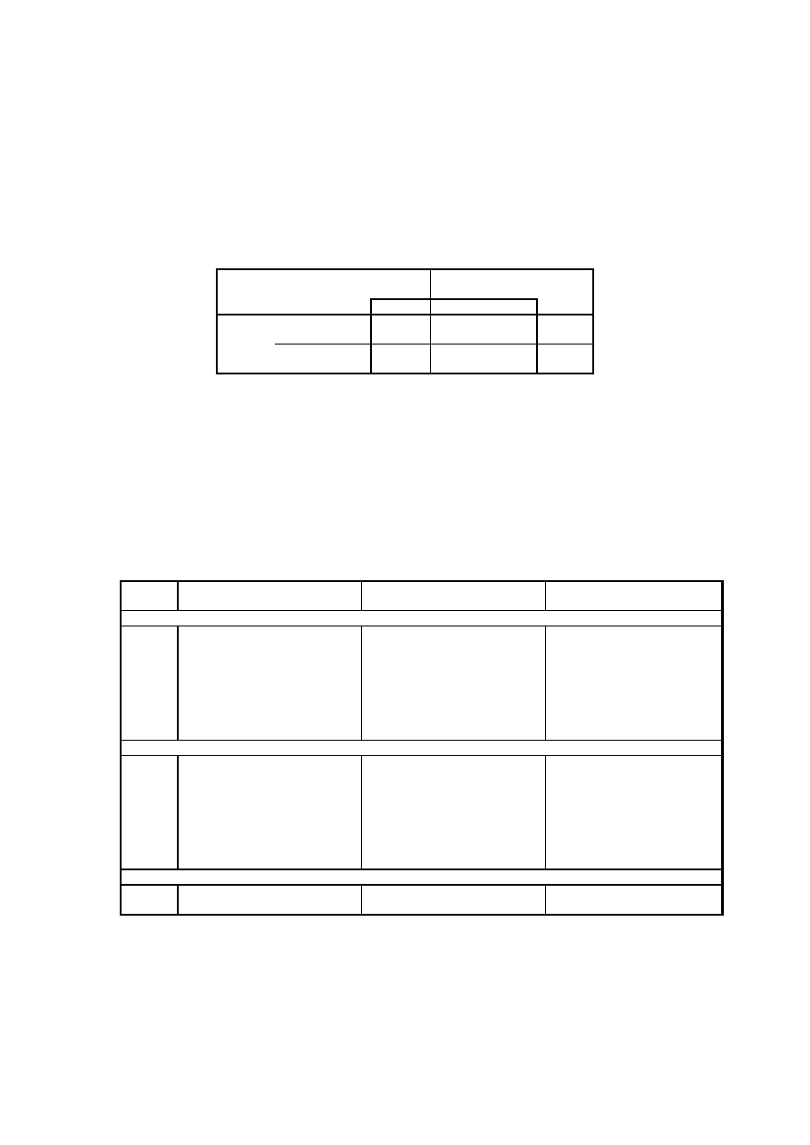
A multivariate ANOVA was carried out on the data of all 9 listeners. Of the pairs that were
repeated in the test, only the second occurrences were used, giving a balanced design. The
results are shown in table 1.

As can be seen, nearly every factor and some interactions are significant to the 0.01 level. If
the most significant factors for each grading scale are taken, then the Width, Depth and
Envelopment factors are mostly dependent on the type of room, and the Naturalness is mostly
dependent on the processor. It is noted that the significance is very high for all of these.

Of most interest are the results of the perceived differences by room and processor. The mean
values and associated 95% confidence intervals by room are shown in figures 9 to 12.

8

The Width, Depth and Envelopment vary in accordance with the size of the room. For all
three of these attributes, the Lexicon Hall is given the highest scores, followed by Studio 1,
with PA 18 being lowest. This is statistically significant in all three cases. These factors are
apparently highly correlated with each other. It is possible that this was caused by the
listeners confusing the scales. However, it is also possible that the correlation between the
spatial attributes is due to the nature of the programme material.

The means and 95% confidence intervals of the Naturalness judgements show much less
separation. Interestingly, for some reason Studio 1 is rated significantly less natural than
PA18. There is no significant difference between the Lexicon Hall and the other two rooms.

Figures 13 to 16 show the mean values and associated 95% confidence intervals of the
judgement data by processor.

For Width, Depth and Envelopment, the processor is not causing the same magnitude of
difference as the rooms, but there are statistically significant differences. Firstly, it appears
that Processor 1 makes the source significantly wider than Processor 3 which is in turn
significantly wider than Processor 2. Secondly, it appears that Processor 2 makes the source
significantly closer than Processor 3. In terms of Envelopment, the subjective result is that
Processors 1 and 3 are significantly more enveloping than Processor 2.

However the most significant result is for Naturalness. This shows Processor 1 to be rated
much lower than the other two. The difference between Processors 2 and 3 is smaller but still
significant. Interestingly, this is the inverse of the rank order of the results for Apparent
Source Width.

Whilst some of the interactions are statistically significant, the associated F-value is more
than a factor of 10 lower than the main factors. Investigation of the significant interactions
reveals that no further useful information can be obtained from this data. Indeed, it has been
said by others that if the difference between the interactions and main factor significance is so
large, it can safely be ignored [26]. In addition, the fact that the interactions are ordinal means
that the main factors are the most important aspects [27].

3.2 Preference analysis

For analysing the preferences, the data from all of the listeners was included. The data was
modified by giving the preferred choice a +1 value and the non-preferred choice a –1 value as
used previously [28, 4]. This was then summed by processor type as shown in figure 17.

It is apparent that Processor 1 is much less preferred than either Processor 2 or Processor 3.
However, whether Processor 2 is significantly preferred over Processor 3 is not so clear. In
fact, the application of a Mann-Whitney U test shows that the difference is significant.

To investigate further, the preference data can be separated out by listener to see if there is
agreement between the subjects or whether it is subject-dependent. This is shown in figure 18.

It is visible that in nearly every case Processor 1 is least preferred compared to the other two
processors. However, it is also apparent that the preference between the other two units is
somewhat subject dependent. Interestingly, those with the strongest preferences (and
therefore possibly most consistent) appear to prefer Processor 2.

Also interesting to note is the similarity between the preference sum separated by processor
(figure 17) and the mean value and 95% confidence intervals of the Naturalness judgements

9

separated by processor as shown earlier (figure 16). This relationship can be explored by the
use of discriminant function analysis.

3.3 Discriminant function analysis

Discriminant function analysis is an extension of the regression types of data analysis. It
attempts to construct a formula that determines the outcome of a grouping variable (in this
case Preference) from a number of other variables (in this case Width, Depth, Envelopment
and Naturalness) [29].

The standardised canonical discriminant function coefficients determine how much influence
each input variable has on the result. These were calculated using the data from all listeners
and are as follows:

•

Apparent Source Width

-0.348

•

Depth

-0.039

•

Envelopment

-0.105

•

Naturalness

1.036

It is clear that Naturalness is the primary factor that is determining preference in this
experiment, with a small negative amount of the Width attribute.

To test the accuracy of this regression model based on the weights shown above, the data was
entered and the results were compared with the original preference data. It is apparent from
table 2 that the resultant equation correctly classified 71.6% of the cases. This is significantly
higher than chance.

3.4 Informal anecdotal information

As a final informal check, the subjects were also asked how many loudspeakers they thought
were in use at most. Out of the 9 listeners, 7 thought that the rear loudspeakers were used for
some extracts. However, all the listeners thought that the front 3 loudspeakers were in use.

3.5

Discussion

Aspects of the spatial quality of three selected virtual home theatre (VHT) systems have been
evaluated by using controlled subjective listening tests. For this case, based on the particular
programme material, listening environment and listening position, the results suggest the
following. Firstly, out of the four attributes tested, the predominant difference that was
perceived between the three VHT algorithms was Naturalness. Secondly, the perceived
differences in Apparent Source Width (ASW), Depth and Envelopment were more affected
by the original environment in the programme material than the processors.

Thirdly, the preference appeared to be based on the perception of Naturalness and a small
negative amount on ASW. Finally, overall, Processor 1 was significantly least preferred and
Processor 2 was most preferred, though this differed somewhat between the listeners.

It appeared from questioning the subjects that Processor 1 suffered from a number of
degrading artefacts that rendered the audio unnatural. The main complaint was that it sounded
out of phase and uncomfortable. Timbral irregularities were also mentioned.

It is recognised that this test may not have high external validity for a number of reasons. The
programme material was limited in this experiment for reasons given in section 1 above. It is
similar to some programme material for which these systems may be used, though does not

10

cover a broad scope of all possible applications. Even so, the results may be applicable across
a wider range of programme material. The subjects were deliberately all experienced
listeners. Whether inexperienced listeners would have preferred the same algorithms as this
group of individuals is open to speculation. Lastly, only one listening position was used in the
test. As it is known that these algorithms are often very position dependent [20], the effect in
other listening positions is of interest.

However, it may be the case that the results found here are externally valid, especially given
the high significance level of the main factors. Indeed, other tests have uncovered similar
results [21].

From these tests, a set of subjective data was generated which was then used to correlate with
objective measures based on the interaural cross-correlation coefficient. It was unfortunate
that the spatial attributes appeared to be so highly correlated with each other. As mentioned
above, this was possibly due to the nature of the programme material used. However, it means
that if a measurement correlates with the spatial attributes, it is unclear whether it would be
only relevant for a single spatial attribute if different programme material was used.

4 Objective measurement using the interaural cross-correlation

coefficient

The interaural cross-correlation coefficient (IACC) is a binaural measure that calculates the
similarity of signals reaching each ear of a listener. The measurements are usually taken over
a fixed window after an impulse (t1 to t2 in equation 1 below). The correlation of these
signals is calculated using the interaural cross-correlation function (IACF). This is expressed
by equation 1.

Equation 1

∫

∫

∫

+

=

2

1

2

1

2

/

1

2

1

]

)

(

)

(

[

]

)

(

)

(

[

)

(

2

2

t

t

t

t

R

L

t

t

R

L

t

dt

t

p

dt

t

p

dt

t

p

t

p

IACF

τ

τ

where p = sound pressure

t = time after the direct sound

R = right ear signal

L = left ear signal [18]

This equation can be derived from the cross-correlation and cross-covariance functions as
shown in [30].

τ

is varied over a time period of ±1ms, a range large enough to encompass the maximum

interaural time difference due to the physical separation of human ears. The result of the
interaural cross-correlation coefficient is the maximum absolute value within the range of

τ

.

This is shown in equation 2.

Equation 2

max

)

(

τ

t

t

IACF

IACC

=

, for –1ms<

τ

<+1ms

[18]

11

A high value indicates that the signals are practically identical and a low value indicates that
the signals are very different. This has been related to subjective perception of concert hall
acoustics such that a low value indicates a diffuse sound field, and a high value, a focused
sound field [31].

Because of its relationship to the interaural time difference, the position of the maximum
value can indicate the direction of sound from the head. In other words, a sound coming from
the right of a listener will reach the right ear before the left ear. This means that the maximum
value will be at a corresponding position related to the respective times of arrival. The
position of the maximum value represents the angle of incidence of the sound from the
median plane [32]. However, this is only very clear for a single source in an anechoic
environment. When the additional reflections of a real room are added, the data becomes
much less defined.

In addition, the end effects of the cross-correlation function must be considered. Without
taking other measures to limit this, the effect can be minimised by:

•

ensuring the window of the sound sample measured (t1 to t2 in equation 1 above) is equal

to or greater than 5 times the period of the lowest frequency component of interest

•

measuring

τ

over a range less than ±20% of the length of the window (t1 to t2) [30]

For example, if frequencies down to 200 Hz are of interest, then the window length must be at
least 25ms. Using this window length,

τ

should be varied over a range less than ±5ms.

4.1 Conventional application of IACC

The IACC measurement can be taken over a range of different windows (t1 to t2 in equation 1
above) from the arrival of an impulse. In the late 1960s, Keet found that a measure
resembling (1 - IACC) with a window of 0 to 50ms was positively correlated with Apparent
Source Width (ASW) for a certain loudness of reproduction [33].

Hidaka et al [18] found that (1 - IACC) with a period of 0 to 80 ms was correlated with
Apparent Source Width and most effective in terms of a larger range of resulting values. This
was based on both previous work and the results of the calculations of their tests. The reason
for including the direct sound is that it results in a larger range of scores in real situations. In
addition, a measurement excluding the direct sound in an anechoic chamber would give an
IACC of 0, an indication of a very uncorrelated signal which is incorrect.

It was also found that the IACC was most effective over three separate octave bands centred
on 500, 1000 and 2000 Hz. Below this, the IACC measurement rose sharply, and above 3000
Hz there was little contribution to ASW [18]. The variant of IACC which Hidaka et al
concluded was most effective was (1 - IACC

E3

), where IACC

E3

was the average of the these

three octave bands of IACC taken over a window of 0 to 80 ms.

Further work found that the physical measure of (1 - IACC

E3

) did correlate with the changes

in the perceived ASW, however this was not accurate across the whole range of parameters
tested [34].

4.2 Measurement details

For the measurements described in this paper, the binaural sound fields were all captured
using a KEMAR head and torso simulator [35]. This was fitted with large ears (DB-065 and
DB-066), Zwislocki occluded ear simulators (DB-100), and Brüel and Kjær 4134
microphones. Binaural recordings were made of all the programme material used in the test.
For this the KEMAR was set up at the listening position in the listening room used in the

12

subjective test. Test signals were also recorded including maximum length sequences (MLS),
impulses, frequency sweeps and noise bursts. These had all been replayed in the acoustic
environments, recorded using 5 discrete channels and processed by the VHT algorithms in the
same manner as the programme material used for the subjective test and described earlier.
This is shown in figure 8.

The IACC measurement was carried out in a number of forms. This included varying the
window period (t1 to t2 in Equation 1 above), and making measurements of the whole
bandwidth, in octave bands, one-third octave bands, and IACC

E3

. Also tested was the result of

cancelling the effect of the occluded ear simulators by filtering the audio with diffuse field
equalisation. The signals measured in each case were the 1 ms pink noise bursts. The reason
for this was that a transient signal was needed to measure appropriate times after the direct
sound, and the impulses had an inadequate signal to noise ratio.

4.3 Correlation with subjective data

As mentioned above, a number of forms of interaural cross-correlation measurement were
attempted. The measured values were then entered into a correlation analysis with the
subjective data. Only the means from the ANOVA analysis were used as the subjective data
because using the raw data proved to be unsuitable for a correlation analysis. The subjective
data used is shown in figures 19 to 22.

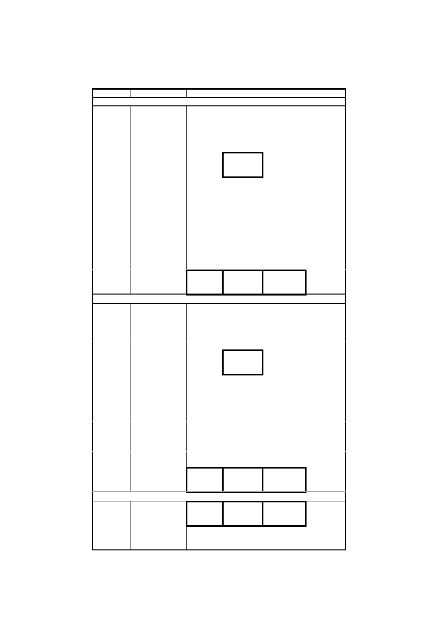
The correlation analysis showed that none of the types of IACC were predictably correlated
with this set of subjective data. As an example, table 3 shows a set of measured results. This
particular set was measured as described above, using a window of 0 to 80ms, and without
diffuse field equalisation. The numbers shown are the results by octave frequency band, first
the raw data, then as 1 - |raw data|. In addition the data for the IACC measured over the whole
audio frequency range is given, along with the IACC

E3

measurement as described above.

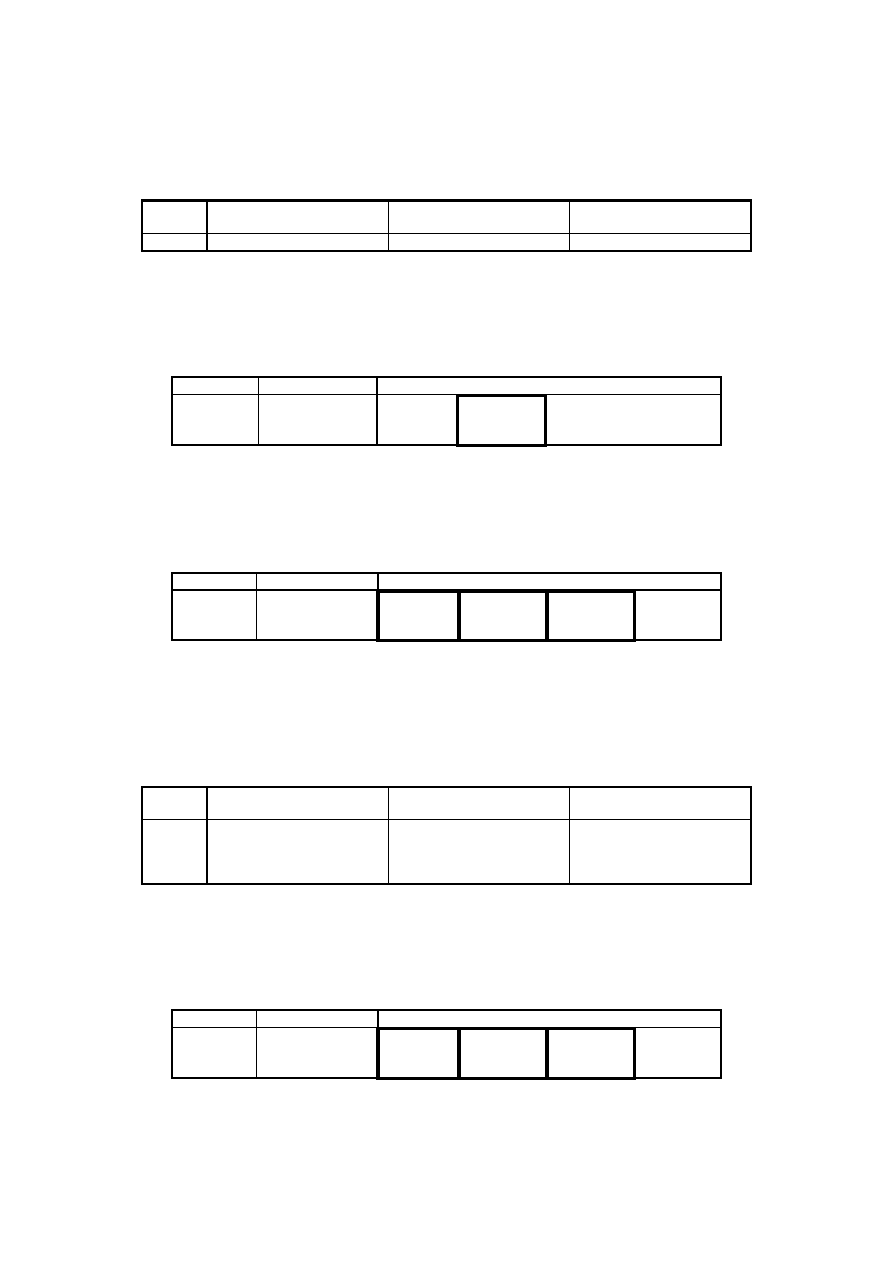
Table 4 shows the correlation matrix of the objective data in table 3 against the subjective
data shown in figures 19 to 22. Statistically significant results can be seen, highlighted by
thick black squares. However, these significant results appear not to support any known
research or theories. Indeed, some of the correlations appear to be negative as opposed to the
positive correlation as found by others and described above. It is not clear why this should be
and the authors can currently offer no explanation.

Therefore, it appears that the IACC measurement is unsatisfactory for reliably predicting any
of the chosen subjective spatial attributes in this case.

5 Objective measurement using the interaural cross-correlation

fluctuation function

A novel measurement was developed, based on the research into IACC as mentioned above,
and the research of Griesinger [36, 37, 10]. This new measure has been named the Interaural
Cross-Correlation Fluctuation Function (IACCFF). This function is a binaural measure and is
based on a consecutive series of IACC calculations. The function measures the fluctuation of
the position of maximum IACC over time. The output is a single value that is the mean of the
fluctuations across a fluctuation rate of 3 to 20 Hz, and an audio frequency range of 50 to
1600 Hz.

13

As the function is only in the very early stages of development, only an overview is provided
here, along with preliminary results that appear encouraging. Further work, including more
details of the function, will be published at a later date.

It was predicted that the IACCFF would measure some aspect of spatial perception. Out of
the three spatial attributes chosen in this experiment, it was expected that the IACCFF would
relate to either Apparent Source Width or Envelopment. This could possibly be dependent on
the type of signal measured (either transient or constant), or how the measurement is
implemented.

5.1 Response to simulations

The measure was initially tested by evaluating its response to extreme conditions for which
the perceived spatial parameters could be estimated.

The first simulation was of the 1ms pink noise burst positioned at 0° elevation and 0° azimuth
from a KEMAR dummy head in an anechoic chamber. This used the KEMAR dummy head
head-related transfer function (HRTF) measurements made by Bill Gardner and Keith Martin
at MIT Media Lab [38].

If the IACCFF measures some form of spatial perception (either ASW or Envelopment as
mentioned above), then it is evident that an anechoic sound field should produce a very low
result. For this signal, the IACCFF gave a result of -Inf (minus infinity), which is very low as
expected.

The second simulation was created using two uncorrelated white noise signals, one fed to the
right ear, the other to the left ear. The subjective result of this was predicted to be a diffuse
sound field [39]. Measuring this sound field using the IACCFF, the result was -9.9625. This
value is significantly higher than for the anechoic simulation as anticipated.

Therefore, it could be concluded that the IACCFF measurement was giving a wide range of
values to the extreme conditions to which it was subjected. In addition, the order of the values
was such that it matched the hypothesis that it was positively related to the subjective spatial
attributes of ASW or Envelopment.

5.2 Correlation with subjective data

The IACCFF was used to measure the binaural recordings of the 1 ms pink noise bursts,
processed as shown in figure 8 and replayed in the listening room. These were the same as
used for the IACC measurement, described above. The results are shown in table 5. A
correlation analysis was performed between this data and the subjective data shown in figures
19 to 22 and as used above. The correlation matrix is shown in table 6. The data for the Depth
attribute is also shown in a scatterplot in figure 23.

It is apparent that the measurement correlates well with the subjective Depth attribute for the
Lexicon Hall and Studio 1 extracts. However, there appears to be a problem with the results
from PA 18. This is likely to be due to the short decay time giving a low signal to noise ratio.
If the data from PA 18 is removed, the correlations between all the spatial attributes and the
IACCFF are much improved as shown in table 7.

In an attempt to use a sound source with a better signal to noise ratio, the snare drum extract
from the programme items was used. This sound is again a wide-bandwidth transient signal,
but this time is a number of separated hits rather than the single noise burst used previously.
The first 5 seconds of the 60 second sound file were measured and the results are shown in
table 8.

14

A correlation analysis was carried out between this data and the subjective data as used above
(figures 19 to 22). The results, shown in table 9 show a high correlation. The scatterplot is
shown in figure 24. It is apparent that the subjective and objective data are now very highly
correlated. However, due to the correlation between the spatial attributes it is not clear if the
function is only relevant for a single perceptual spatial dimension or for all of them.

6 Discussion

To summarise, three virtual home theatre (VHT) algorithms were tested using subjective
methods. They were also measured using a number of objective methods based on the
interaural cross-correlation (IACC) function, and these were compared with the subjective
results.

It appears that in this case the IACC does not predict any of the subjective spatial attributes
tested. Interestingly, the diffuse field equalisation made a very small difference to the
measured results, contrary to the findings of Morimoto and Iida [40]. The reason for the poor
performance of the IACC measure may be due to the artificial nature of the programme
material used in this experiment. Even so, for a measure to be an optimum representation of a
subjective attribute, it should be reliable regardless of the stimulus. Therefore, although the
IACC measurement has proved useful in concert hall acoustics, it appears that in this case it is
not a satisfactory solution.

The interaural cross correlation fluctuation function (IACCFF) appears to correlate much
better with the subjective results in this case. However, whether the measure will be
successful in other experiments is yet to be tested. As mentioned above, the correlation
between the spatial attributes in the subjective results means that it is impossible to ascertain
whether the measure is only relevant for one particular spatial attribute. So far, little is known
about the function and its particular qualities, and further research needs to be done to refine
the scope and definition of the measure.

Ideally, a useful measurement would be able to take the inputs of a known loudspeaker
configuration, and give a representative output for any given programme material. Currently
the IACCFF is a long way from this ideal. Measurements of binaural recordings of the
programme material used in the listening test resulted in unsatisfactory results. For the
measurement to achieve this ideal, an improved binaural model is needed, including improved
filter banks, analysis of subjective loudness, a simulation of the precedence effect, and
substantial research into the effects of continuous and transient signals. In addition some
consideration of the source segmentation or streaming as discussed by Bregman [41] may be
necessary.

Consideration must also be given to other aspects of subjective testing. The subjects
themselves are influenced by other factors from outside the test that each individual subject
brings with them. In addition, factors within the test, such as interaction between audio and
visual stimuli have been proven to affect the perception of either [42]. An objective measure
may not take all of these into account, and therefore can only give at best a ‘mean opinion
score’ (MOS) rather than exactly matching the results of a single subject. Even so, these
results are useful as a guide, and similar models for other aspects of audio quality have
already been standardised [43, 44].

In addition, specific implementation problems with the IACCFF need to be addressed. These
include only being able to measure single sources located in the median plane, and the result
being dependent on the sound source duration.

15

However, the initial results from this experiment are encouraging and warrant further
investigation.

7 Conclusion

To summarise, by using controlled subjective listening tests, the results suggest the following
for this particular case:

•

Out of the four attributes tested, the predominant perceived difference between the three

VHT processors is Naturalness

•

The perceived differences in ASW, Depth and Envelopment are more affected by the

original environments in the programme material than the processors

•

Preference is mainly based on the perception of Naturalness and a small negative amount

on ASW

•

Overall, Processor 1 is significantly least preferred and Processor 2 most preferred,

though this is somewhat listener dependent

The result of objective tests using measurements based on IACC suggest the following for
this particular case:

•

The IACC does not appear to produce results that correlate well with any of the chosen

subjective spatial attributes used in this experiment

•

The IACCFF appears to correlate quite strongly with all three of the chosen subjective

spatial attributes for certain test and programme signals

Further details of the measurement and further experimental results will be reported in due
course.

Acknowledgements

The authors would like to thank David Meares and BBC R&D for sponsorship and provision
of equipment, the MEDUSA team for their thought-provoking discussions and guidance, Nick
Cutmore and Roger Brownless at the BBC for assistance in the anechoic chamber, Dr. Tim
Brookes for assistance with DSP and MATLAB, Søren Bech and Dr. Bart de Bruyn for their
comments on the paper, the AES Educational Foundation for financial assistance and Lin
Oskam for her patient proof reading.

16

Appendix A -Instructions for listeners

The purpose of this listening test is to judge a number of audio extracts. The audio will be reproduced
from any of up to 5 loudspeakers in the room. The test is run on the GuineaPig test software that you
will control with a mouse via the graphical user interface. On the screen will be four buttons: ‘A’; ‘B’;
‘stop’; and ‘Done’. Clicking on either ‘A’ or ‘B’ will start the audio, clicking ‘stop’ will stop the audio,
and clicking ‘Done’ will move you to the next test item.

The test is of an A - B form. This means that there will be two concurrent sources that you can switch
between at any time. To do this, use the mouse to click on the buttons A or B to switch to the
corresponding source. Each extract is 60 seconds long. During this time you are free to switch as many
or as few times as you wish. If you have not made a decision in this time, clicking on either A or B will
start the audio again. You have as much time as you feel you need to take.

You are asked to grade each audio extract on 4 criteria. These are: image size; depth of image;
envelopment; and naturalness. These can be described as:

•

image size – how narrow / wide or focused / diffuse is the sound source?

•

depth of image – how far away do you perceive the sound source to be?

•

envelopment – how enveloping is the audio? Is it all around or is it limited to the front speakers?

•

naturalness – how natural is the audio? How realistic and free from degrading artefacts is it?

The scales are:

0

10

narrow / focused ------------------------------------- wide / diffuse
close ---------------------------------------------------- far / deep
sound only in front -------------------------------------- enveloping
unnatural --------------------------------------------------- natural

The endpoints denote the extremes of the scales.

The grading is done by clicking and dragging the bar in the grading scale to the desired point. The
numerical grades are shown on the scale in order to guide you. Grades can be made at any point on the
line, not just at the integer points. You are asked to grade both sources A and B. The grading however
is not to be a comparison between the two sources, but grading on an absolute scale. You are also asked
to give a preference by clicking on either A or B underneath the grading scale. The computer will not
let you grade the items until both have been heard, and will not let you move to the next item until the
grade has been given.

It is important to remember that there is no right or wrong answer. Your judgement is the correct
answer and you will not be marked on your choices. You will not be told anything about the sources
involved or the processing carried out, if any. If you are interested, you can find out after all the
listening tests have been carried out.

To repeat: I am looking for your evaluation of the sources. The sources are to be compared and grades
made in terms of their image width, image depth, envelopment, and naturalness. The grading scale is
from far left to far right, with the extremes being at each end. The preference indication is the choice
that you find most aesthetically pleasing.

Please feel free to ask any questions, preferably before the test begins.

Enjoy the listening, and thank you for taking part.

45

17

References

[1] Grewin, Christer. 1995: ‘Can Objective Measures Replace Subjective Assessments?’,

Audio Engineering Society Preprints, 99

th

Convention, preprint no. 4067.

[2] Rumsey, Francis 1998: ‘Subjective assessment of the spatial attributes of reproduced

sound’, Proceedings of the 15

th

International Audio Engineering Society Conference,

Copenhagen, Denmark, pp. 122-135.

[3] Beranek, Leo. 1996: Concert and Opera Halls – how they sound, (Woodbury, NY:

Acoustical Society of America).

[4] Schroeder, M. R., Gottlob, D. and Siebrasse, K. F. 1974: ‘Comparative study of European

concert halls: correlation of subjective preference with geometric and acoustic parameters’,
Journal of the Acoustical Society of America, vol. 56, no. 4 (October), pp. 1195-1201.

[5] Ando, Yoichi. 1985: Concert Hall Acoustics, Berlin: Springer-Verlag.

[6] Kurozumi, Kohichi and Ohgushi, Kengo. 1983: ‘The relationship between the cross-

correlation coefficient of two-channel acoustic signals and sound image quality’, Journal
of the Acoustical Society of America, vol. 74, no. 6 (December), pp. 1726-1733.

[7] Bareham, John R. 1996: ‘Measurement of Spatial Characteristics of Sound Reproduced in

Listening Spaces’, Audio Engineering Society Preprint, 101

st

Convention, preprint no.

4381.

[8] Martin, Geoff, Woszczyk, Wieslaw, Corey, Jason and Quesnel, René. 1999: ‘Controlling

Phantom Image Focus in a Multichannel Reproduction System’, Audio Engineering
Society Preprint, 107

th

Convention, preprint no. 4996.

[9] Griesinger, David. 1997: ‘The Psychoacioustics of Apparent Source Width, Spaciousness

and Envelopment in Performance Spaces’, Acta Acustica, vol. 83, no. 4 (July/August), pp.
721-731.

[10] Griesinger, David. 1998: ‘General Overview of Spatial Impression, Envelopment,

Localization, and Externalization’, Proceedings of the 15

th

International Audio

Engineering Society Conference, Copenhagen, Denmark, pp. 136-149.

[11] Zacharov, Nick, Huopaniemi, Jyri and Hämäläinen, Matti. 1999: ‘Results of a Round

Robin Subjective Evaluation of Virtual Home Theatre Sound Systems’, Audio
Engineering Society Preprint, 107

th

Convention, preprint no. 5067.

[12] Berg, Jan and Rumsey, Francis. 1999: ‘Spatial Attribute Identification and Scaling by

Repertory Grid Technique and other methods’, Proceedings of the 16

th

International

Audio Engineering Society Conference, Rovaniemi, Finland, pp. 51-66.

[13] Morimoto, Masayuki. 1997: ‘The Role of Rear Loudspeakers in Spatial Impression’,

Audio Engineering Society Preprint, 103

rd

Convention, preprint no. 4554.

[14] Yamaguchi, Kiminori. 1972: Multivariate analysis of subjective and physical measures

of hall acoustics, Journal of the Acoustical Society of America, vol. 52, pp. 1271-1279.

18

[15] Hansen, Villy and Munch, Gert. 1991: ‘Making Recordings for Simulation Tests in the

Archimedes Project’, Journal of the Audio Engineering Society, vol. 39, no. 10
(October), pp. 768-774.

[16] Olive, Sean E., Schuck, Peter L., Sally, Sharon L. and Bonneville, Marc E. 1994: ‘The

Effects of Loudspeaker Placement on Listener Preference Ratings’, Journal of the Audio
Engineering Society, vol. 42, no.9 (September), pp. 651–669.

[17] More details can be found at http://www.mlssa.com.

[18] Hidaka, Takayuki, Beranek, Leo L. and Okano, Toshiyuki. 1995: ‘Interaural cross-

correlation, lateral fraction, and low- and high-frequency sound levels as measures of
acoustical quality in concert halls’, Journal of the Acoustical Society of America, vol.
98, no. 2 (August), pp. 988-1007.

[19] Walker, Robert. 1999: ‘A Simple Acoustic Room Model for Virtual Production’,

Proceedings of the 1999 Audio Engineering Society UK Conference – Audio: the
second century, London, pp. 48-72.

[20] Olive, Sean E. 1998: ‘Subjective Evaluation of 3-D Sound Based on Two Loudspeakers’,

Proceedings of the 15

th

International Audio Engineering Society Conference,

Copenhagen, Denmark, pp. 194-210.

[21] Zacharov, Nick, Huopaniemi, Jyri and Hämäläinen, Matti. 1999: ‘Round Robin

Subjective Evaluation of Virtual Home Theatre Surround Systems at the AES 16

th

International Conference’, Proceedings of the 16

th

International Audio Engineering

Society Conference, Rovaniemi, Finland, pp. 544-556.

[22] Hynninen, J. and Zacharov N. 1999: ‘GuineaPig - A Generic Subjective Test System for

Multichannel Audio’, Audio Engineering Society Preprint, 106

th

Convention, preprint

no. 4871.

[23] ITU-R BS 1116. 1994: ‘Methods for the Subjective Assessment of Small Impairments in

Audio Systems including Multichannel Sound Systems’, International
Telecommunications Union, Recommendations ITU-R BS 1116, pp. 276-297.

[24] Moore, Brian C. J., Glasberg, Brian R. and Baer, Thomas. 1997: ‘A Model for the

Prediction of Thresholds, Loudness, and Partial Loudness’, Journal of the Audio
Engineering Society, vol. 45, no. 4 (April), pp. 224-240.

[25] Software available from: http://hearing.psychol.cam.ac.uk/Demos/demos.html.

[26] Bech, Søren. 1999: Personal communication with the authors.

[27] Hair, Joseph F., Anderson, Rolph E., Tatham, Ronald L. and Black, William C. 1995:

Multivariate Data Analysis with Readings, (New Jersey: Prentice Hall).

[28] Mason, Russell and Rumsey, Francis. 1999: ‘An investigation of Microphone

Techniques for Ambient Sound in Surround Sound Systems’, Audio Engineering
Society Preprint, 106

th

Convention, preprint no. 4912.

19

[29] Tabachnick, Barbara G. and Fidell, Linda S. 1996: Using Multivariate Statistics, (New

York: Harper Collins).

[30] Ifeachor, Emmanuel C. and Jervis, Barrie W. 1993: Digital Signal Processing: A

Practical Approach, (Wokingham, UK: Addison-Wesley).

[31] Ando, Yoichi and Kurihara, Yoshitaka. 1986: ‘Nonlinear response in evaluating the

subjective diffuseness of sound fields’, Journal of the Acoustical Society of America,
vol. 80, no. 3 (September), pp. 833-836.

[32] Blauert, J. and Cobben, W. 1978: ‘Some Consideration of Binaural Cross Correlation

Analysis’, Acustica, vol. 39, pp. 96-104.

[33] Keet, Wilhelm de Villiers. 1968: ‘The Influence of Early Lateral Reflections on the

Spatial Impression’, 6

th

International Congress on Acoustics, Tokyo, Japan, pp. E53-

E56.

[34] Okano, Toshiyuki, Beranek, Leo L. and Hidaka, Takayuki. 1998: ‘Relations among

interaural cross-correlation coefficient (IACC

E

), lateral fraction (LF

E

), and apparent

source width (ASW) in concert halls’, Journal of the Acoustical Society of America,
vol. 104, no. 1 (July), pp. 255-265.

[35] Burkhard, M. D. and Sachs, R. M. 1975: ‘Anthropometric manikin for acoustic

research’, Journal of the Acoustical Society of America, vol. 58, no. 1 (July), pp. 214-
222.

[36] Griesinger, David. 1992a: ‘IALF – Binaural Measures of Spatial Impression and

Running Reverberance’, Audio Engineering Society Preprint, 92

nd

Convention, preprint

no. 3292.

[37] Griesinger, David. 1992b: ‘Measures of Spatial Impression and Reverberance Based on

the Physiology of Human Hearing’, Proceedings of the 11

th

International Audio

Engineering Society Conference, Portland, Oregon, USA, pp. 114-145.

[38] Gardner, Bill and Martin, Keith. 1994: ‘HRTF Measurements of a KEMAR Dummy-

Head Microphone’, http://sound.media.mit.edu/~kdm/hrtf.html.

[39] Kendall, Gary S. 1995: ‘The Decorrelation of Audio Signals and Its Impact on Spatial

Imagery’, Computer Music Journal, vol. 19, no. 4 (Winter), pp.71-87.

[40] Morimoto, Masayuki and Iida, Kazuhiro. 1995: ‘A practical evaluation method of

auditory source width in concert halls’, Journal of the Acoustical Society of Japan
(English Translation), vol. 16, no. 2, pp. 59-69.

[41] Bregman, Albert S. 1990: Auditory Scene Analysis: the perceptual organization of

sound, (Cambridge, MA: MIT Press).

[42] Beerends, John G. and De Caluwe, Frank E. 1999: ‘The Influence of Video Quality on

Perceived Audio Quality and Vice Versa’, Journal of the Audio Engineering Society,
vol. 47, No. 5 (May) pp. 355-362.

[43] ITU-R BS 1387. 1999: ‘Method for objective measurements of perceived audio quality’,

International Telecommunications Union, Recommendations ITU-R BS 1387.

20

[44] Colomes, Catherine, Schmidmer, Christian, Thiede, Thilo and Treurniet, William C.

1999: ‘Perceptual Quality Assessment for Digital Audio: PEAQ – The new ITU standard
for objective measurement of the perceived audio quality’, Proceedings of the 17

th

International Audio Engineering Society Conference, Florence, Italy, pp. 114-145.

45

21

Tables

Table 1: Multivariate ANOVA results table for all listeners with ASW, Depth,

Envelopment and Naturalness as dependent variables and subject (SUBJECNO),
processor (PROCNO), room (ROOMNO) and musical excerpt (EXCERPNO) as
fixed factors.

Source

Dependent

Variable

Type III Sum of

Squares

df

Mean Square

F

Sig.

SUBJECNO

ASW

955.2332

8

119.404147

95.074940

0.0000

Depth

907.3990

8

113.424877

103.461881

0.0000

Envelopment

811.9025

8

101.487816

91.297190

0.0000

Naturalness

684.2323

8

85.529032

53.911668

0.0000

PROCNO

ASW

56.0858

2

28.042886

22.329004

0.0000

Depth

31.9319

2

15.965941

14.563528

0.0000

Envelopment

123.3921

2

61.696034

55.500993

0.0000

Naturalness

344.4571

2

172.228534

108.561122

0.0000

ROOMNO

ASW

267.2530

2

133.626497

106.399413

0.0000

Depth

586.4528

2

293.226404

267.470031

0.0000

Envelopment

657.5041

2

328.752052

295.741299

0.0000

Naturalness

21.7874

2

10.893719

6.866658

0.0012

EXCERPNO

ASW

4.3181

3

1.439383

1.146101

0.3306

Depth

11.3393

3

3.779774

3.447767

0.0170

Envelopment

24.1656

3

8.055201

7.246359

0.0001

Naturalness

72.8360

3

24.278657

15.303610

0.0000

SUBJECNO *

ASW

95.1470

16

5.946688

4.735020

0.0000

PROCNO Depth

28.9451

16

1.809066

1.650162

0.0551

Envelopment

100.2765

16

6.267284

5.637971

0.0000

Naturalness

211.5607

16

13.222544

8.334590

0.0000

SUBJECNO *

ASW

353.5456

16

22.096601

17.594305

0.0000

ROOMNO Depth

332.2375

16

20.764842

18.940903

0.0000

Envelopment

421.3428

16

26.333927

23.689677

0.0000

Naturalness

125.9712

16

7.873198

4.962727

0.0000

PROCNO *

ASW

20.0647

4

5.016173

3.994102

0.0035

ROOMNO Depth

70.2018

4

17.550455

16.008861

0.0000

Envelopment

11.5700

4

2.892492

2.602050

0.0360

Naturalness

5.3947

4

1.348673

0.850111

0.4943

SUBJECNO *

ASW

67.2234

32

2.100730

1.672696

0.0149

PROCNO * Depth

43.5329

32

1.360403

1.240908

0.1793

ROOMNO Envelopment

43.5898

32

1.362180

1.225400

0.1929

Naturalness

69.5175

32

2.172423

1.369347

0.0933

SUBJECNO *

ASW

69.4644

24

2.894348

2.304610

0.0006

EXCERPNO Depth

45.8701

24

1.911255

1.743375

0.0181

Envelopment

130.1865

24

5.424437

4.879757

0.0000

Naturalness

149.8219

24

6.242581

3.934897

0.0000

PROCNO *

ASW

8.7625

6

1.460417

1.162849

0.3259

EXCERPNO Depth

5.4180

6

0.902999

0.823681

0.5522

Envelopment

10.1247

6

1.687454

1.518013

0.1715

Naturalness

57.0875

6

9.514583

5.997344

0.0000

SUBJECNO *

ASW

45.1925

48

0.941510

0.749673

0.8877

PROCNO * Depth

39.6784

48

0.826633

0.754024

0.8829

EXCERPNO Envelopment

49.3344

48

1.027801

0.924597

0.6179

Naturalness

74.0125

48

1.541927

0.971926

0.5300

ROOMNO *

ASW

15.2182

6

2.536373

2.019574

0.0627

EXCERPNO Depth

21.7171

6

3.619511

3.301581

0.0036

Envelopment

8.5656

6

1.427608

1.284259

0.2639

Naturalness

18.3534

6

3.058904

1.928125

0.0758

SUBJECNO *

ASW

130.5543

48

2.719880

2.165691

0.0000

ROOMNO * Depth

71.7960

48

1.495750

1.364366

0.0634

EXCERPNO Envelopment

109.6719

48

2.284830

2.055405

0.0001

Naturalness

102.6124

48

2.137758

1.347497

0.0714

PROCNO *

ASW

11.3222

12

0.943519

0.751272

0.7005

ROOMNO * Depth

13.8942

12

1.157852

1.056149

0.3970

EXCERPNO Envelopment

13.7781

12

1.148171

1.032881

0.4180

Naturalness

22.8752

12

1.906265

1.201580

0.2805

Error

ASW

406.9100

324

1.255895

Depth

355.2000

324

1.096296

Envelopment

360.1650

324

1.111620

Naturalness

514.0150

324

1.586466

22

Table 2: Discriminant Function Analysis summary table for regression model based on

factors of ASW, Depth, Envelopment and Naturalness shown in section 3.3 to
predict grouping variable Preference from subjective experiment data.

Predicted Group
Membership

Total

Preference -1

1

Original

Count

-1

231

93

324

1

91

233

324

%

-1

71.3

28.7

100.0

1

28.1

71.9

100.0

71.6% of original grouped cases correctly classified.

Table 3: Results of IACC measurements made of 1 ms pink noise burst processed as

shown in figure 8 and recorded in listening room with KEMAR head using a
window of 0 to 80 ms without diffuse field equalisation.

Processor

1

1

1

2

2

2

3

3

3

Room

Lexicon

PA 18

Studio 1

Lexicon

PA 18

Studio 1

Lexicon

PA 18

Studio 1

Octave-band centred on:

63

0.79889

0.88297

0.98286

0.99091

0.98097

0.99014

0.84571

0.85478

0.99458

125

0.40607

0.6284

0.93946

0.93667

0.92386

0.97124

0.5425

0.44531

0.95678

250

0.20087

-0.15871

0.85754

0.42544

0.76217

0.92486

-0.19221

0.18745

0.85571

500

0.66809

0.46349

0.28936

-0.42719

0.61314

0.55605

0.45394

-0.13815

0.58695

1000

0.43674

0.30914

-0.20835

-0.33579

0.47914

0.42793

-0.38789

0.28498

0.42324

2000

-0.22473

-0.43454

-0.50093

0.43387

0.59453

-0.51577

-0.53136

-0.63636

-0.41627

4000

-0.55632

-0.57227

0.61808

0.47186

0.64292

0.57489

0.20698

0.31931

0.57085

8000

0.2695

0.36724

0.48899

-0.21864

0.31462

0.60142

0.29781

0.24461

0.48498

1 - |IACC| octave band centred on :

63

0.20111

0.11703

0.01714

0.00909

0.01903

0.00986

0.15429

0.14522

0.00542

125

0.59393

0.3716

0.06054

0.06333

0.07614

0.02876

0.4575

0.55469

0.04322

250

0.79913

0.84129

0.14246

0.57456

0.23783

0.07514

0.80779

0.81255

0.14429

500

0.33191

0.53651

0.71064

0.57281

0.38686

0.44395

0.54606

0.86185

0.41305

1000

0.56326

0.69086

0.79165

0.66421

0.52086

0.57207

0.61211

0.71502

0.57676

2000

0.77527

0.56546

0.49907

0.56613

0.40547

0.48423

0.46864

0.36364

0.58373

4000

0.44368

0.42773

0.38192

0.52814

0.35708

0.42511

0.79302

0.68069

0.42915

8000

0.7305

0.63276

0.51101

0.78136

0.68538

0.39858

0.70219

0.75539

0.51502

Wide bandwidth

1-IACC

0.67372

0.65143

0.47966

0.75753

0.49528

0.46644

0.71475

0.63794

0.49036

1-IACC

E3

0.6625

0.6663

0.707

0.6762

0.4573

0.5187

0.6151

0.6759

0.5407

23

Table 4: Pearson correlation analysis between IACC measurement results shown in

table 3 and subjective results shown in figures 19 to 22.

Width

Depth

Envelopment Naturalness

Octave band IACC centred on :

63 Hz

Pearson Correlation

0.222112

0.589185

0.324599

0.418494

Sig. (2-tailed)

0.565709

0.095026

0.394076

0.26228

N

9

9

9

9

125 Hz

Pearson Correlation

0.208676

0.575112

0.308702

0.390452

Sig. (2-tailed)

0.590014

0.105214

0.418942

0.298827

N

9

9

9

9

250 Hz

Pearson Correlation

0.458162

0.668726

0.459844

0.218151

Sig. (2-tailed)

0.214881

0.048908

0.212984

0.572835

N

9

9

9

9

500 Hz

Pearson Correlation

0.33992

0.136772

0.279884

-0.3266

Sig. (2-tailed)

0.370779

0.725677

0.465745

0.390995

N

9

9

9

9

1000 Hz

Pearson Correlation

0.370179

0.231682

0.232126

-0.22488

Sig. (2-tailed)

0.326771

0.548627

0.547838

0.56074

N

9

9

9

9

2000 Hz

Pearson Correlation

-0.63137

-0.38383

-0.64489

0.445172

Sig. (2-tailed)

0.0682

0.307814

0.060747

0.229841

N

9

9

9

9

4000 Hz

Pearson Correlation

0.13749

0.441984

0.231642

0.630053

Sig. (2-tailed)

0.724283

0.233596

0.548698

0.068957

N

9

9

9

9

8000 Hz

Pearson Correlation

0.824176

0.67599

0.786335

-0.37717

Sig. (2-tailed)

0.00629

0.045619

0.011961

0.316988

N

9

9

9

9

1 - |IACC| octave band centred on :

63 Hz

Pearson Correlation

-0.222112

-0.589185

-0.324599

-0.418494

Sig. (2-tailed)

0.565709

0.095026

0.394076

0.26228

N

9

9

9

9

125 Hz

Pearson Correlation

-0.208676

-0.575112

-0.308702

-0.390452

Sig. (2-tailed)

0.590014

0.105214

0.418942

0.298827

N

9

9

9

9

250 Hz

Pearson Correlation

-0.490571

-0.722047

-0.529842

-0.230994

Sig. (2-tailed)

0.179975

0.028045

0.142328

0.549848

N

9

9

9

9

500 Hz

Pearson Correlation

0.22387

0.19126

0.25434

-0.100559

Sig. (2-tailed)

0.56255

0.622046

0.508993

0.796861

N

9

9

9

9

1000 Hz

Pearson Correlation

0.36347

0.28727

0.40888

-0.440158

Sig. (2-tailed)

0.336298

0.453548

0.274527

0.235762

N

9

9

9

9

2000 Hz

Pearson Correlation

-0.114377

-0.288971

-0.141617

-0.403994

Sig. (2-tailed)

0.769518

0.450754

0.716278

0.280869

N

9

9

9

9

4000 Hz

Pearson Correlation

-0.425133

-0.475788

-0.355623

0.33163

Sig. (2-tailed)

0.253993

0.195468

0.347603

0.383304

N

9

9

9

9

8000 Hz

Pearson Correlation

-0.773842

-0.879908

-0.796474

0.12323

Sig. (2-tailed)

0.014402

0.001754

0.010197

0.752122

N

9

9

9

9

Wide bandwidth

1 - IACC all Pearson Correlation

-0.756811

-0.79102

-0.731657

0.09861

freq bands Sig. (2-tailed)

0.018236

0.011123

0.025053

0.800743

N

9

9

9

9

1 – IACC

E3

Pearson Correlation

0.019952

-0.16193

0.027166

-0.51078

Sig. (2-tailed)

0.959367

0.67724

0.944693

0.159964

N

9

9

9

9

24

Table 5: Results of IACCFF measurements made of 1 ms pink noise burst processed as

shown in figure 8 and recorded in listening room with KEMAR head.

Processor

1

1

1

2

2

2

3

3

3

Room

PA 18

Studio 1

Lexicon

PA 18

Studio 1

Lexicon

PA 18

Studio 1

Lexicon

IACCFF

-30.7614 -22.1295 -18.9857 -21.0363 -25.3765 -18.1478 -24.3318 -24.0451 -20.9018

Table 6: Pearson correlation analysis between IACCFF measurement results shown in

table 5 and subjective results shown in figures 19 to 22.

Width

Depth

Envelopment

Naturalness

IACCFF

Pearson Correlation

0.458572

0.774789

0.582951

0.210705

Sig. (2-tailed)

0.214418

0.014206

0.099461

0.58632

N

9

9

9

9

Table 7: Pearson correlation analysis between IACCFF measurement results shown in

table 5 excluding results for PA 18 and subjective results shown in figures 19 to 22.

Width

Depth

Envelopment

Naturalness

IACCFF

Pearson Correlation

0.887746

0.947098

0.837306

-0.19705

Sig. (2-tailed)

0.018194

0.004124

0.037551

0.708246

N

6

6

6

6

Table 8: Results of IACCFF measurements made of first 5 seconds of Snare Drum

extract of programme material processed as shown in figure 8 and recorded in
listening room with KEMAR head.

Processor

1

1

1

2

2

2

3

3

3

Room

PA 18

Studio 1

Lexicon

PA 18

Studio 1

Lexicon

PA 18

Studio 1

Lexicon

IACCFF

of Snare

Drum

excerpts

-16.3577 -13.3362

-11.219 -18.3394 -16.4946 -11.9289 -17.6494 -13.4884 -12.2604

Table 9: Pearson correlation analysis between IACCFF measurement results shown in

table 8 and subjective results shown in figures 19 to 22.

Width

Depth

Envelopment

Naturalness

IACCFF of

Pearson Correlation

0.981263

0.881938

0.973777

-0.46722

Snare Drum Sig. (2-tailed)

2.91E-06

0.001656

9.37E-06

0.204773

Excerpts N

9

9

9

9

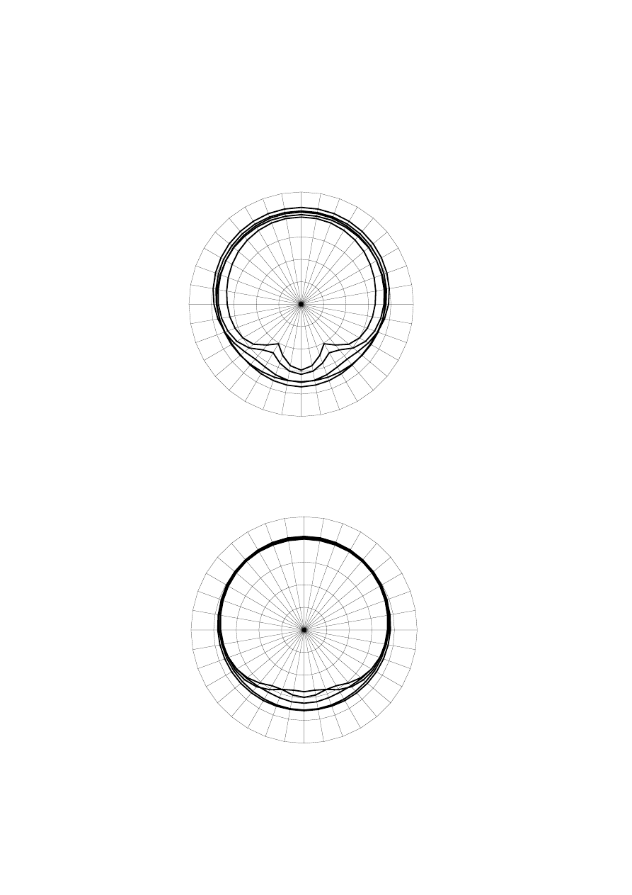
25

Figures

Figure 1: Polar response of Rogers LS 5/8 at frequencies of 75, 150, 225, 300, and 370

Hz.

-20

-10

0

10

20

30

0

10

20

30

40

50

60

70

80

90

100

110

120

130

140

150

160

170

180

190

200

210

220

230

240

250

260

270

280

290

300

310

320

330

340

350

Figure 2: Polar response of B&W 801 at frequencies of 75, 150, 225, 300, and 370 Hz.

-20

-10

0

10

20

30

0

10

20

30

40

50

60

70

80

90

100

110

120

130

140

150

160

170

180

190

200

210

220

230

240

250

260

270

280

290

300

310

320

330

340

350

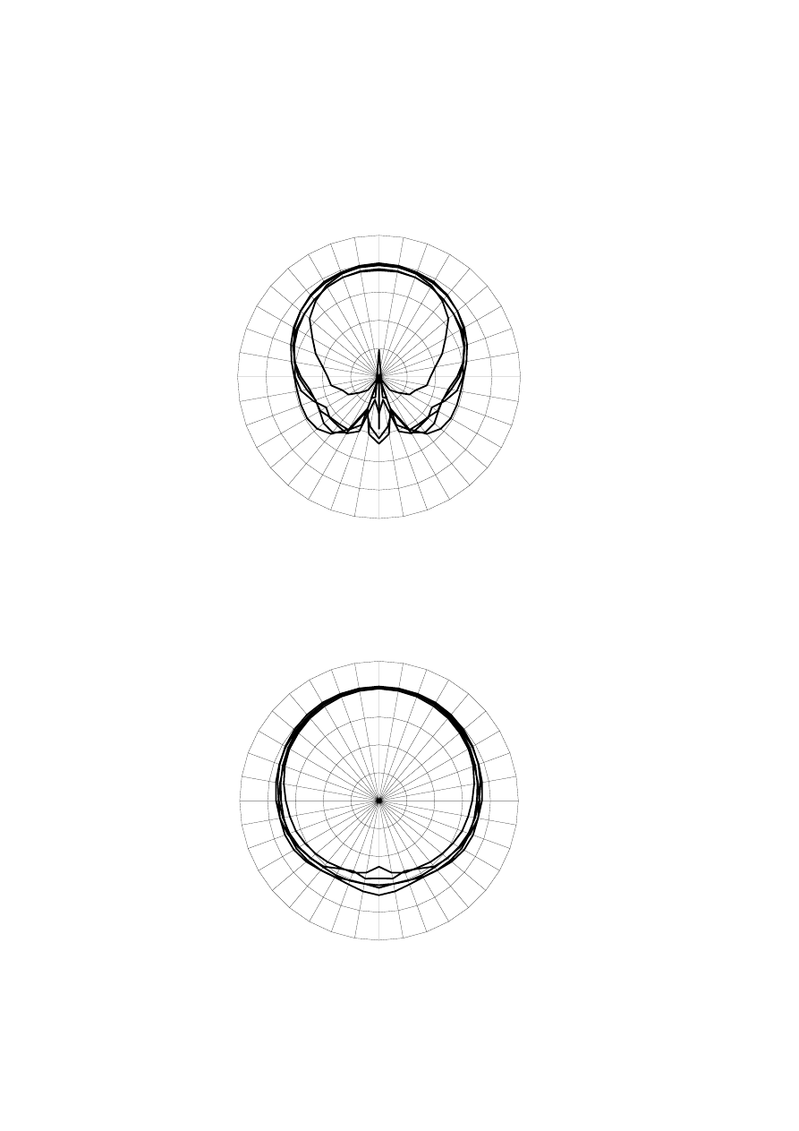
26

Figure 3: Polar response of Rogers LS 5/8 at frequencies of 520, 660, 810, 1030, and 1250

Hz.

-20

-10

0

10

20

30

0

10

20

30

40

50

60

70

80

90

100

110

120

130

140

150

160

170

180

190

200

210

220

230

240

250

260

270

280

290

300

310

320

330

340

350

Figure 4: Polar response of B&W 801 at frequencies of 520, 660, 810, 1030, and 1250 Hz.

-20

-10

0

10

20

30

0

10

20

30

40

50

60

70

80

90

100

110

120

130

140

150

160

170

180

190

200

210

220

230

240

250

260

270

280

290

300

310

320

330

340

350

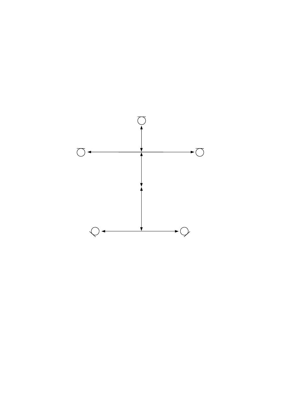
27

Figure 5: Diagram of 5-channel microphone array consisting of Neumann KM-84

cardioid microphones. Rear channel microphones on-axis direction was pointed 45°
away from directly backwards.

1.60 m

1.01 m

0.34 m

0.52 m

0.53 m

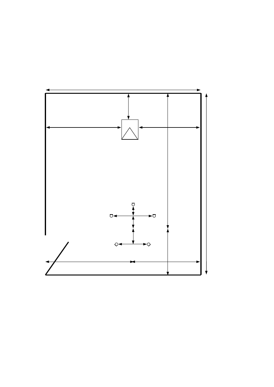
28

Figure 6: Diagram of microphone layout in PA 18.

3.01m

6.08 m

2.64m

3.25 m

2.83 m

4.92 m

3.08 m

8.00 m

1.32 m

1.60 m

1.01 m

0.34 m

0.52 m

0.53 m

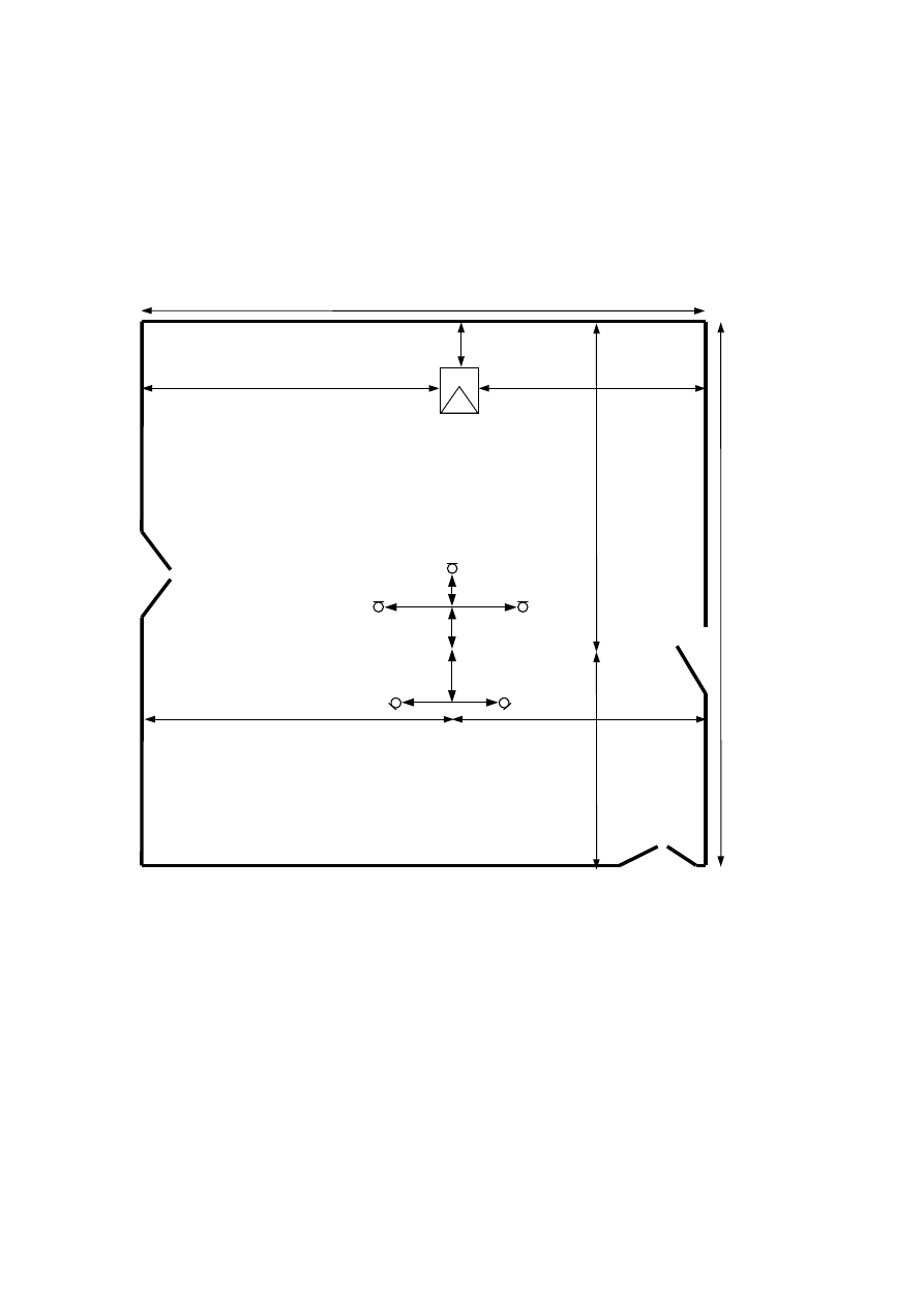
29

Figure 7: Diagram of microphone layout in Studio 1.

14.36 m

2.14 m

7.23 m

6.70 m

7.30 m

7.06 m

9.02 m

8.02 m

17.04 m

1.60 m

1.01 m

0.34 m

0.52 m

0.53 m

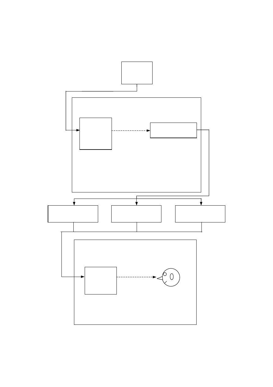
30

Figure 8: Block diagram of processing, both electronic and acoustic (denoted by dashed

lines) carried out on anechoic recordings and test signals.

Replay

anechoic

recording

Acoustic environment

Loudspeaker

Discrete 5-channel

capture

Virtual home theatre

processor 1

Virtual home theatre

processor 2

Virtual home theatre

processor 3

Replay in listening room

5 – channel

loudspeaker

array

Head

(human or KEMAR)

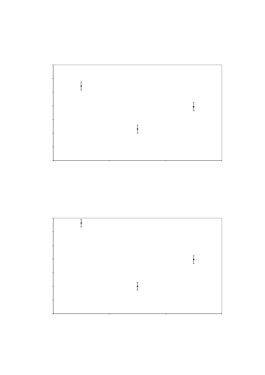
31

Figure 9: Mean value and the associated 95% confidence intervals of Apparent Source

Width judgements averaged across all listeners separated by Room as generated by
the ANOVA model.

2.5

3

3.5

4

4.5

5

5.5

6

Lexicon hall

PATS PA18

PATS studio 1

Room

Apparent source width judgements

Figure 10: Mean value and the associated 95% confidence intervals of Depth

judgements averaged across all listeners separated by Room as generated by the
ANOVA model.

2.5

3

3.5

4

4.5

5

5.5

6

Lexicon hall

PATS PA18

PATS studio 1

Room

Depth judgements

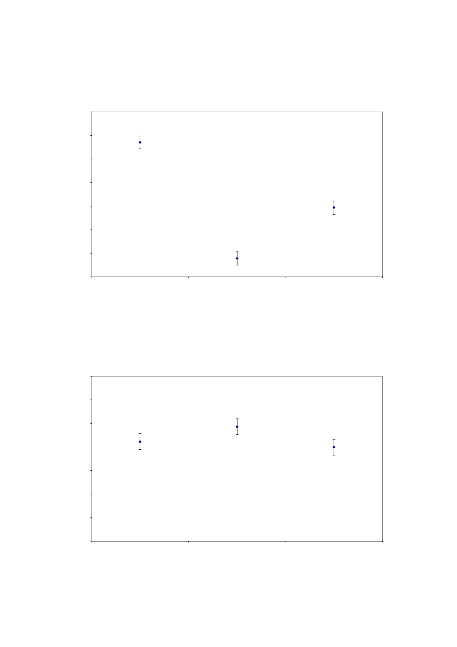
32

Figure 11: Mean value and the associated 95% confidence intervals of Envelopment

judgements averaged across all listeners separated by Room as generated by the
ANOVA model.

2.5

3

3.5

4

4.5

5

5.5

6

Lexicon hall

PATS PA18

PATS studio 1

Room

Envelopment judgements

Figure 12: Mean value and the associated 95% confidence intervals of Naturalness

judgements averaged across all listeners separated by Room as generated by the
ANOVA model.

2.5

3

3.5

4

4.5

5

5.5

6

Lexicon hall

PATS PA18

PATS studio 1

Room

Naturalness judgements

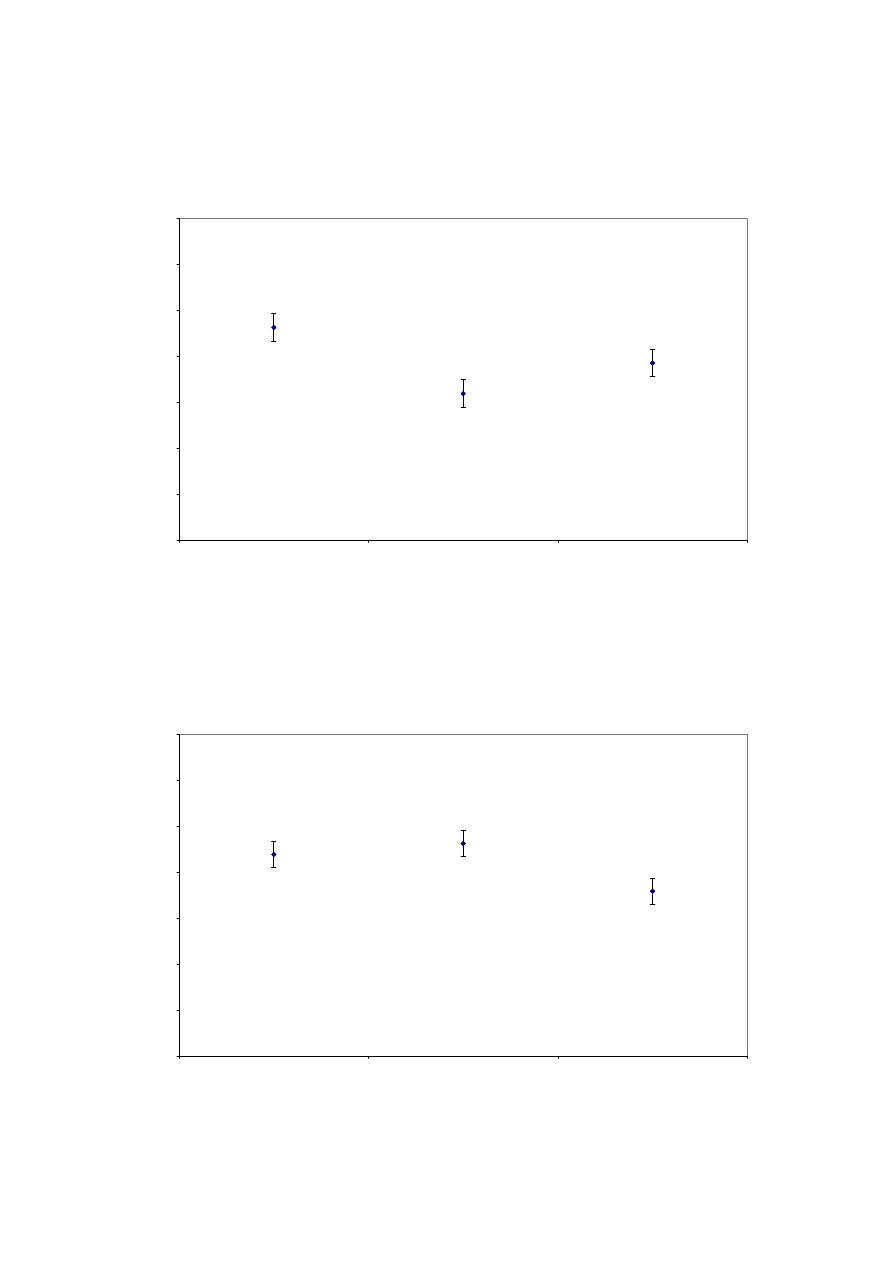
33

Figure 13: Mean value and the associated 95% confidence intervals of Apparent Source

Width judgements averaged across all listeners separated by Processor as generated
by the ANOVA model.

2.5

3

3.5

4

4.5

5

5.5

6

Processor 1

Processor 2

Processor 3

Processor

Apparent source width judgements

Figure 14: Mean value and the associated 95% confidence intervals of Depth

judgements averaged across all listeners separated by Processor as generated by the
ANOVA model.

2.5

3

3.5

4

4.5

5

5.5

6

Processor 1

Processor 2

Processor 3

Processor

Depth judgements

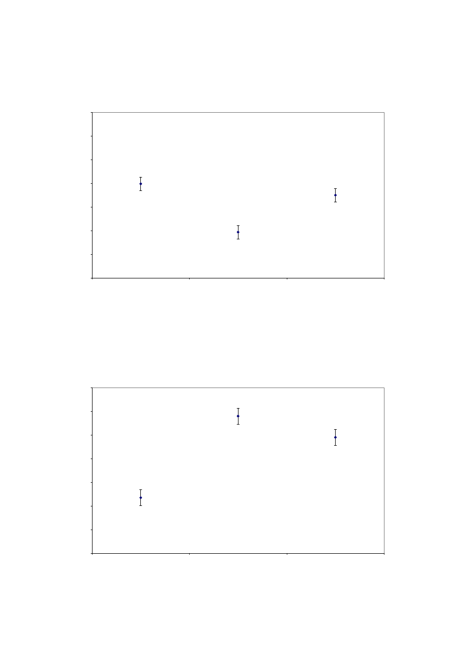
34

Figure 15: Mean value and the associated 95% confidence intervals of Envelopment

judgements averaged across all listeners separated by Processor as generated by the
ANOVA model.

2.5

3

3.5

4

4.5

5

5.5

6

Processor 1

Processor 2

Processor 3

Processor

Envelopment judgements

Figure 16: Mean value and the associated 95% confidence intervals of Naturalness

judgements averaged across all listeners separated by Processor as generated by the
ANOVA model.

2.5

3

3.5

4

4.5

5

5.5

6

Processor 1

Processor 2

Processor 3

Processor

Naturalness judgements

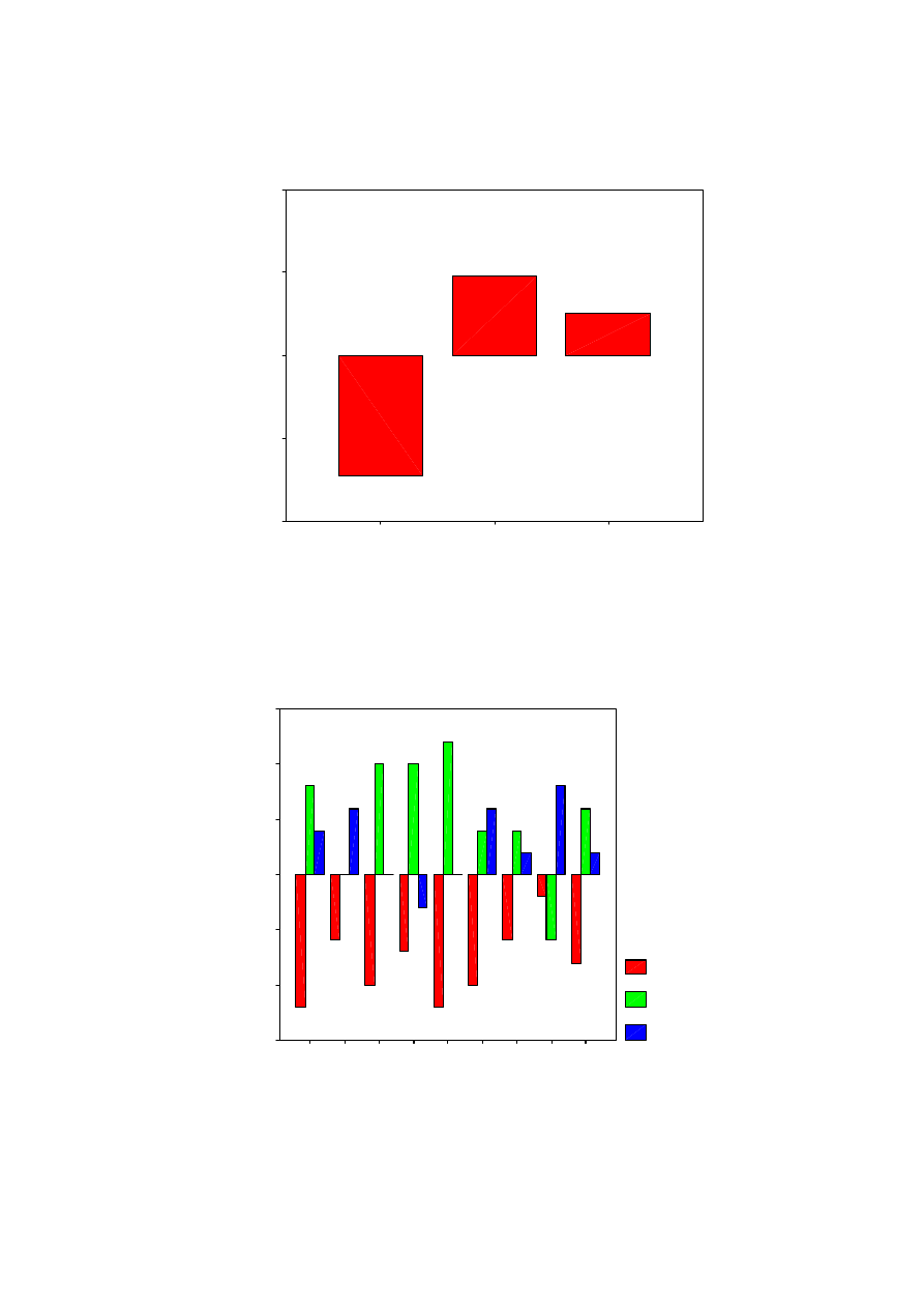
35

Figure 17: Sum of preference data for al listeners separated by Processor.

Processor

Processor 3

Processor 2

Processor 1

Sum Preference

200

100

0

-100

-200

Figure 18: Sum of preference data for all listeners separated by Processor and Subject.

Subject Number

9

8

7

6

5

4

3

2

1

Sum Preference

30

20

10

0

-10

-20

-30

Processor

Processor 1

Processor 2

Processor 3

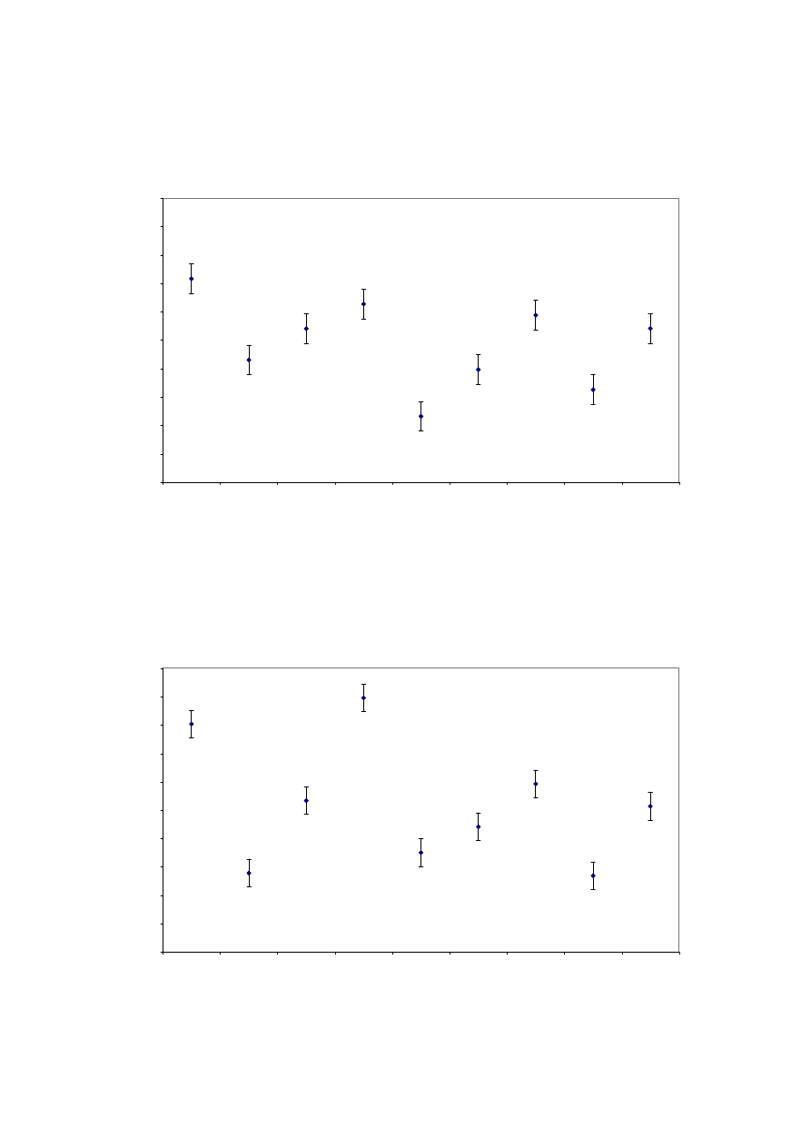
36

Figure 19: Mean value and the associated 95% confidence intervals of Apparent Source

Width judgements averaged across all listeners separated by Processor and Room as
generated by the ANOVA model.

2

2.5

3

3.5

4

4.5

5

5.5

6

6.5

7

Lexicon hall
Processor 1

PATS PA18

PATS studio 1

Lexicon hall

Processor 2

PATS PA18

PATS studio 1

Lexicon hall

Processor 3

PATS PA18

PATS studio 1

Room

Apparent Source Width judgements

Figure 20: Mean value and the associated 95% confidence intervals of Depth

judgements averaged across all listeners separated by Processor and Room as
generated by the ANOVA model.

2

2.5

3

3.5

4

4.5

5

5.5

6

6.5

7

Lexicon hall
Processor 1

PATS PA18

PATS studio 1

Lexicon hall

Processor 2

PATS PA18

PATS studio 1

Lexicon hall

Processor 3

PATS PA18

PATS studio 1

Room

Depth judgements

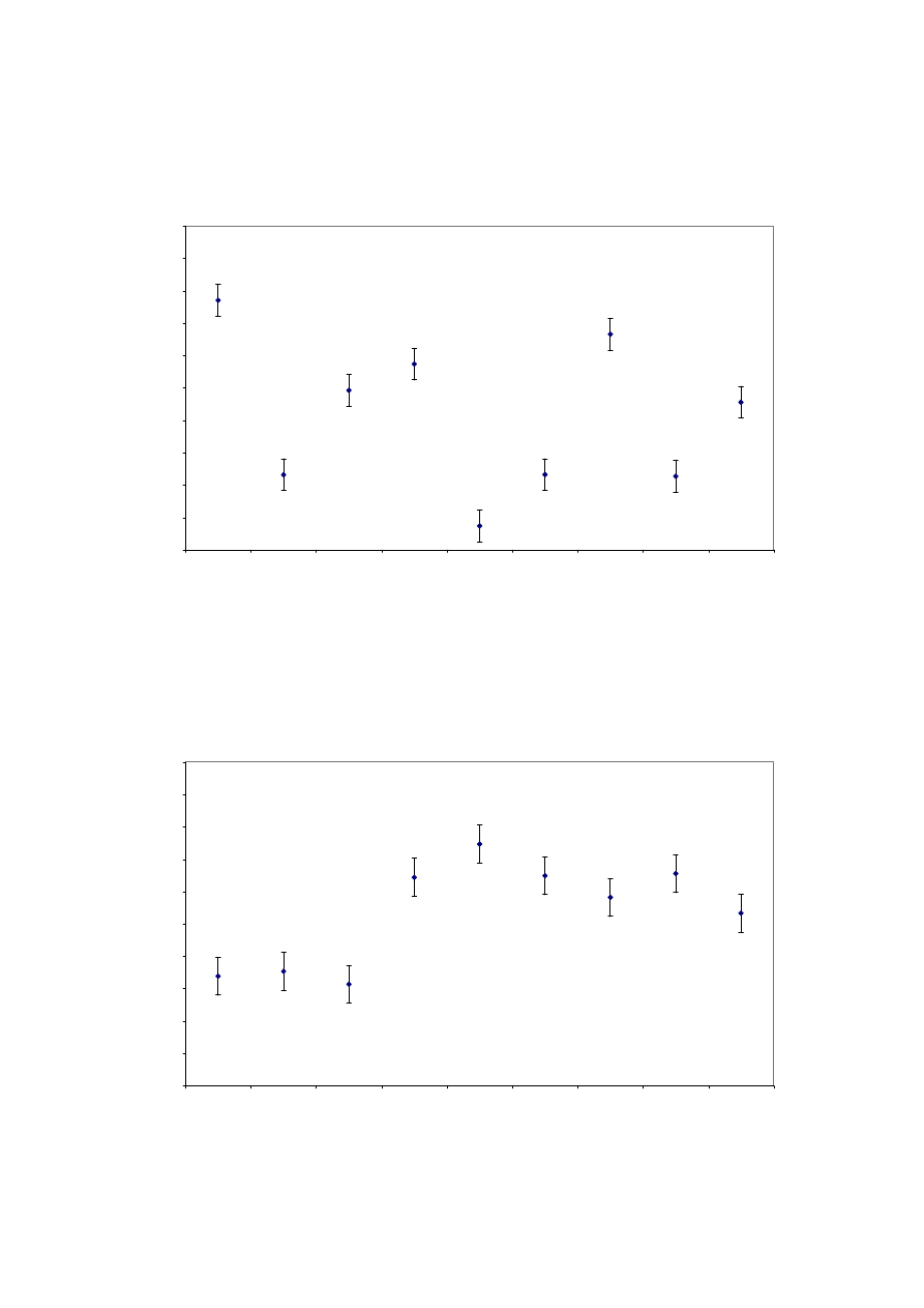
37

Figure 21: Mean value and the associated 95% confidence intervals of Envelopment

judgements averaged across all listeners separated by Processor and Room as
generated by the ANOVA model.

2

2.5

3

3.5

4

4.5

5

5.5

6

6.5

7

Lexicon hall
Processor 1

PATS PA18

PATS studio 1

Lexicon hall

Processor 2

PATS PA18

PATS studio 1

Lexicon hall

Processor 3

PATS PA18

PATS studio 1

Room

Envelopment judgements

Figure 22: Mean value and the associated 95% confidence intervals of Naturalness

judgements averaged across all listeners separated by Processor and Room as
generated by the ANOVA model.

2

2.5

3

3.5

4

4.5

5

5.5

6

6.5

7

Lexicon hall
Processor 1

PATS PA18

PATS studio 1

Lexicon hall

Processor 2

PATS PA18

PATS studio 1

Lexicon hall

Processor 3

PATS PA18

PATS studio 1

Room

Naturalness judgements

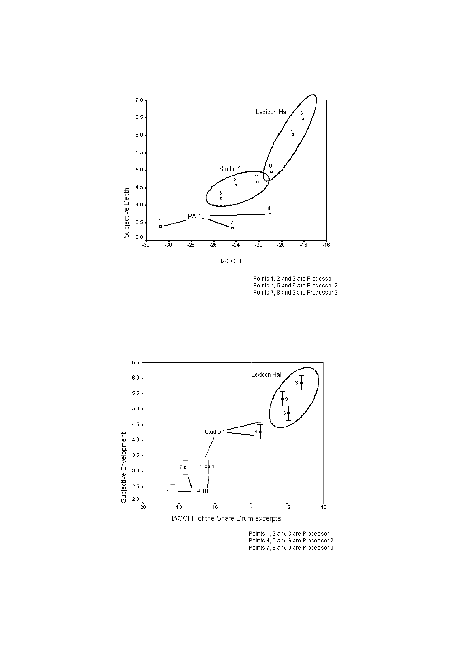
38

Figure 23: Scatter plot of IACCFF measurement results shown in table 5 against

subjective data for the Depth attribute shown in figure 20.

Figure 24: Scatter plot of IACCFF measurement results shown in table 8 against

subjective data for the Envelopment attribute shown in figure 21.