Modeling for Control of HCCI Engines

Gregory M. Shaver

Design Division

Dept. of Mechanical Engineering

Stanford University

Stanford, California 94305-4021

Email: [e-mail]

J.Christian Gerdes

Design Division

Dept. of Mechanical Engineering

Stanford University

Stanford, California 94305-4021

Email: [e-mail]

Parag Jain

Design Division

Dept. of Mechanical Engineering

Stanford University

Stanford, California 94305-4021

Email: [e-mail]

P.A. Caton

Thermosciences Division

Dept. of Mechanical Engineering

Stanford University

Stanford, California 94305-4021

Email: [e-mail]

C.F. Edwards

Thermosciences Division

Dept. of Mechanical Engineering

Stanford University

Stanford, California 94305-4021

Email: [e-mail]

Abstract

The goal of this work is to accurately predict the phasing
of HCCI combustion for a single cylinder research engine
using variable valve actuation (VVA) at Stanford Univer-
sity. Three simple single-zone models were developed and
compared with experiment.

The difference between the

three modeling approaches centered around the combustion
chemistry mechanism used in each. The first modeling ap-
proach, which utilized a temperature threshold to model the
onset of the combustion reaction, did not work well. How-
ever, an integrated reaction rate threshold accounting for
both the temperature and concentration did correlate well
with experiment. Additionally, another model utilizing a
simple two-step kinetic mechanism also showed good cor-
relation with experimental combustion phasing.

1 Introduction

Experimental studies at Stanford University ([1], [4]) and
elsewhere [6] demonstrate that variable valve actuation
(VVA) can be used to initiate homogeneous charge com-
pression ignition (HCCI). This is achieved by reinducting
combustion products from the previous cycle, thereby in-
creasing the sensible energy of the reactant charge and al-
lowing ignition to occur by compression alone at modest
compression ratios. Since the reinducted products act as
a thermal sink during combustion, this process lowers the
peak combustion temperature, which in turn lowers NOx
concentrations. This drop in NOx is one of the major bene-

fits of HCCI. It is important to note that other methods exist
to initiate HCCI, such as heating or precompressing the in-
take air ([10],[7]) or varying the compression ratio [2].

Due to the nature of HCCI, a fundamental control chal-
lenge exists. Unlike spark ignition (SI) or diesel engines,
where the combustion is initiated via spark and fuel injec-
tion, respectively, HCCI has no specific event that initiates
combustion. Therefore, ensuring that combustion occurs
with acceptable timing is more complicated than in the case
of either SI or diesel combustion. HCCI combustion tim-
ing is dominated by chemical kinetics, which depends on
in-cylinder species concentrations, temperature and pres-
sure. These parameters are controlled in the system studied
through the use of the fully flexible VVA system.

To synthesize a controller to stabilize HCCI using the VVA
system, a model of the system with special attention paid
to combustion phasing is therefore necessary. This model
should be as simple as possible, as it is often difficult to
synthesize controllers from more complex models. This pa-
per describes three fairly simple models and compares them
to behavior seen on a single-cylinder research engine out-
fitted with a fully flexible VVA system. Each model tracks
the in-cylinder pressure, temperature and species concentra-
tions during an HCCI cycle. The complete cycle includes
the concurrent induction of the reactants through the intake
valve and the products of combustion from the previous cy-
cle through the exhaust valve, compression, expansion and
exhaust. The valve flow during the induction and exhaust
portions of the cycle are modeled with compressible, steady
state, one-dimensional, isentropic flow relations. The three

models differ only in the approach used to model the com-
bustion chemistry. In the first model, the simplest of the
three, a temperature threshold is used to model the onset
of combustion. This approach shows poor correlation with
experiment, failing to capture the dependence of combus-
tion timing on concentration. In the second model, a two
step mechanism implementing a series of Arrhenius reac-
tion rates is used. Good correlation with experiment with
respect to phasing is found, with slight discrepancy in pres-
sure at the initiation of combustion. The third model imple-
ments elements from the other two models through the use
of an integrated Arrhenius rate as a threshold value. This ap-
proach shows good correlation with experiment, but shows
slight discrepancy as combustion completes.

Various types of models of HCCI combustion with more
complexity than those presented here have been devel-
oped. These include multi-zone models ([8], [3]) and multi-
dimensional CFD models [5]. While these approaches can
be expected to more accurately predict the performance and
emissions in HCCI combustion, the goal of this work is to
develop simple models characterizing combustion phasing.
It is from the simplified models that controllers may more
readily be synthesized to stabilize the HCCI combustion
during load tracking.

2 Modeling Approach

For each of the three approaches investigated, the model-
ing was based on an open system first law analysis, with
steady state compressible flow relations used to model the
mass flow through the intake and exhaust valves. The model
includes nine states: the temperature, T; the concentrations
of propane, [C

3

H

8

], oxygen, [O

2

], Nitrogen, [N

2

], carbon

dioxide, [C

2

O], water, [H

2

O], and carbon monoxide, [CO];

the crank angle,

θ

; and the cylinder volume, V.

2.1 Volume Rate Equation
The in-cylinder volume and its derivative are given by the
following well-known slider-crank formulas:

V

= V

c

+

π

B

2

4

(l − a − acos

θ

−

p

l

2

− a

2

sin

2

θ

) (1)

˙

V

=

π

4

B

2

a ˙

θ

sin

θ

(1 + a

cos

θ

p(L

2

− a

2

sin

2

θ

)

)

(2)

with:

˙

θ

=

ω

(3)

where

ω

is the rotational speed of the crankshaft, a is half

of the stroke length, L is the connecting rod length, B is the
bore diameter and V

c

is the clearance volume at top dead

center.

2.2 Valve Flow Equations
The mass flow through the valves consists of flow from
intake manifold to cylinder, ˙

m

1

, from cylinder to exhaust

manifold, ˙

m

2

, and from exhaust manifold to cylinder, ˙

m

3

,

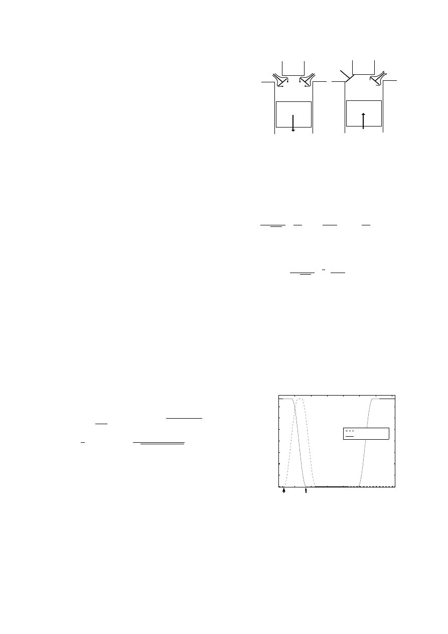
as shown in Figure 1.

Equations for these mass flow

INTAKE
VALVE

EXHAUST
VALVE

m

1

.

m

2

.

EXHAUST
VALVE

m

3

.

INTAKE
VALVE

-

Figure 1:

Valve Mass Flows: left - induction with intake and

exhaust valves open, right - exhaust

rates are developed using a compressible, steady state,
one-dimensional, isentropic flow analysis for a restriction,
where real gas flow effects are included by means of a dis-
charge coefficient, C

D

. The relations for the mass flows are:

˙

m

=

C

D

A

R

p

o

√

RT

o

p

T

p

o

1

/

γ

"

2

γ

γ

− 1

"

1 −

p

T

p

o

(

γ

−1)/

γ

##

(4)

for unchoked flow (p

T

/p

o

> [2/(

γ

+ 1)]

γ

/(

γ

−1)

), and:

˙

m

=

C

D

A

R

p

o

√

RT

o

√

γ

2

γ

+ 1

(

γ

+1)/2(

γ

−1)

(5)

for choked flow (p

T

/p

o

≤[2/(

γ

+1)]

γ

/(

γ

−1)

), where A

R

is the

effective open area for the valve, p

o

is the upstream stagna-

tion pressure, T

o

is the downstream stagnation temperature

and p

T

is the downstream stagnation pressure.

Figure 2 shows the general shape of a valve area profile
used for comparison between model and experiment. It
is the intake valve opening (IVO) and exhaust valve clos-
ing (EVC) locations that are varied for different operating
conditions. For the mass flow of the reactant gas into the

0

100

200

300

400

500

600

700

0

1

2

3

4

5

6

7

8

x 10

−4

Effective Open Area [m]

Crankshaft

°

Intake Valve
Exhaust Valve

IVO

EVC

Figure 2: General Valve Profile

cylinder through the intake valve, ˙

m

1

, p

o

is the intake man-

ifold pressure, assumed to be atmospheric, and p

T

is the

cylinder pressure, p. For the mass flow of burnt products

out of the cylinder through the exhaust valve, ˙

m

2

, p

o

is the

cylinder pressure, p, and p

T

is the exhaust manifold pres-

sure, assumed to be atmospheric. For the reinducted ex-
haust from the previous cycle through the exhaust valve, ˙

m

3

,

p

o

is the exhaust manifold pressure, and p

T

is the cylinder

pressure,p. Setting the manifold pressure to atmospheric is
an approximation. Strategies to model manifold flow dy-
namics are available [9], and could be implemented here in
a straightforward way to describe manifold pressure fluc-
tuations. Note that it is assumed that there is no flow from
cylinder to intake manifold. This is a reasonable assumption
for the experimental system studied in this paper. However,
allowing flow from cylinder to intake manifold is straight-
forward if desired.

2.3 Concentration Rate Equations
The rate of change of concentration for species i, [ ˙

X

i

] is

related to number of moles of species i in the cylinder, N

i

,

by:

˙

[X

i

] =

d

dt

N

i

V

=

˙

N

i

V

−

˙

V N

i

V

2

= w

i

−

˙

V N

i

V

2

(6)

where w

i

, the rate of change of moles of species i per unit

volume has been defined as:

w

i

=

˙

N

i

V

(7)

It has two contributions: the rate of change of moles of
species i per unit volume due to the combustion reactions,
w

rxn

,i

, and due to flow through the valves under the control

of the VVA system, w

valves

,i

, such that:

w

i

= w

rxn

,i

+ w

valves

,i

(8)

The combustion reaction rate, w

rxn

,i

, is determined through

the use of a combustion chemistry mechanism. As noted,
the mechanism used is the difference between the three
models presented in this paper. These approaches will be
outlined in Section 3.

Given the mass flow rates ( ˙

m

1

, ˙

m

2

and ˙

m

3

) from the analysis

in Section 2.2, the rate of change of moles of species i per
unit volume due to flow through the valves, w

valves

,i

, can be

found using the species mass fractions:

w

valves

,i

= w

1

,i

+ w

2

,i

+ w

3

,i

(9)

where:

w

1

,i

=

Y

1

,i

˙

m

1

V MW

i

(10)

w

2

,i

=

Y

2

,i

˙

m

2

V MW

i

(11)

w

3

,i

=

Y

3

,i

˙

m

3

V MW

i

(12)

Here Y

1

,i

, Y

2

,i

and Y

3

,i

are the mass fractions of species i in

the inlet manifold, exhaust manifold and cylinder, respec-
tively. It is assumed that a stoichiometric mixture is present

in the intake manifold. Further, it is assumed that only the
major combustion products of CO

2

, H

2

O and N

2

are re-

inducted into the cylinder through the exhaust. Therefore

Y

1

,i

and Y

2

,i

are constant. Note that other intake and exhaust

manifold compositions can be considered, but in any case
the manifold mass fractions are constant during an engine
cycle. However, the mass fraction of species i in the cylin-
der, Y

3

,i

, is constantly changing, and can be related to the

concentration states as:

Y

3

,i

=

[X

i

]MW

i

∑

[X

i

]MW

i

(13)

2.4 Temperature Rate Equations
In order to derive a differential equation for the temperature
of the gas inside the cylinder, the first law of thermodynam-
ics for an open system and the ideal gas law are combined
as outlined below. The first law of thermodynamics for an
open system is:

d

(mu)

dt

= Q −W + ˙

m

1

h

1

+ ˙

m

2

h

2

+ ˙

m

3

h

3

(14)

where m is the mass of species in the cylinder, u is the in-
ternal energy, Q is the heat transfer rate, W is the work, h

1

is the enthalpy of species in the intake manifold, h

2

is the

enthalpy of species in the exhaust manifold, and h

3

is the

enthalpy of the species in the cylinder. For the case of the
piston cylinder the work is:

W

= p ˙

V

(15)

where

ν

is the specific volume of the gas in the cylinder.

Now, given that the enthalpy is related to the internal energy
as:

h

= u + p

ν

(16)

Equations 14,15 and 16 can be combined to yield:

d

(mh)

dt

= ˙

mpV

/m + ˙pV + ˙

m

1

h

1

+ ˙

m

2

h

2

+ ˙

m

3

h

3

(17)

Expansion of the enthalpy to show the contributions of the
species in the cylinder can be represented as:

mh

= H =

∑

N

i

ˆh

i

(18)

where N

i

is the number of moles of species i in the cylin-

der, and H is the total enthalpy of species in Joules in the
cylinder, and ˆh

i

is the enthalpy of species i on a molar basis.

Noting that the rate of change of enthalpy per unit mole of

species i can be represented as

˙ˆh

i

= c

p

,i

(T ) ˙

T , where c

p

,i

(T )

is the specific heat of species i per mole at temperature T ,
Equations 18 and 6 can be combined to give:

d

(mh)

dt

= V

∑

˙

[X

i

]ˆh

i

+ ˙

T

∑

[X

i

]c

p

,i

(T )

+ ˙

V

∑

[X

i

]ˆh

i

(19)

In-cylinder pressure and its derivative can be related to the
concentrations and temperature through the ideal gas law
as:

p

=

∑

[X

i

]RT

(20)

˙

p

=

p

∑

˙

[X

i

]

∑

[X

i

]

+

p ˙

T

T

(21)

Meanwhile, the in cylinder mass and its derivative may be
related to the species concentrations, molecular weights and
volume as:

m

= V

∑

[X

i

]MW

i

(22)

˙

m

=

˙

V

∑

[X

i

]MW

i

+V

∑

˙

[X

i

]MW

i

(23)

Equating the right sides of Equations 17 and 19, substituting
Equations 21, 22, and 23, and rearranging yields a differen-
tial equation for temperature:

˙

T

=

−(

∑

˙

[X

i

]ˆh

i

) −

˙

V

(

∑

[X

i

]ˆh

i

)

V

+

p

∑

˙

[X

i

]

∑

[X

i

]

+

∑

˙

m

i

h

i

V

(

∑

[X

i

] ˆc

p

,i

(T )) − p/T

(24)

Equations 2, 3, 6 and 24 represent the set of nonlinear dif-
ferential equations for each of the nine states used in each
of the models.

As noted, the combustion reaction rate,

w

rxn

,i

, in Equation 6 is modeled differently in each of the

approaches as outlined in the next section.

3 Combustion Chemistry Modeling

The combustion chemistry mechanism utilized is the differ-
ence between the three modeling approaches. For all three
approaches, the stoichiometric reaction of propane and air
is assumed since this is the case for the experimental data
for which model results are compared. The major products
assumption is also made, such that the global reaction for
combustion can be written as:

C

3

H

8

+ 5O

2

+ 18.8N

2

→ 3CO

2

+ 4H

2

O

+ 18.8N

2

(25)

3.1 Temperature Threshold Approach
As a first pass a simple temperature threshold method was
developed in which the combustion reactions are assumed
to start once the in-cylinder temperature reaches a critical
value. In this case, the rate of reaction of the propane is
approximated as being gaussian in nature, such that:

w

C

3

H

8

=











[C

3

H

8

]

i

V

i

˙

θ

exp

h

−((

θ

−

θ

init )−

¯

θ

)

2

σ

2

i

V

σ

√

2

π

T ≥ T

th

0

T

< T

th











(26)

where

θ

init

, V

i

and

[C

3

H

8

]

i

are the crank angle, volume and

propane concentration, respectively, at the point where com-
bustion begins (i.e. where T

= T

th

). Further,

σ

and ¯

θ

are the

standard deviation and mean associated with the gaussian

reaction rate expression, and are fitted to correlate with ex-
periment at one operating condition. Note that other func-
tions could be used to model the reaction rate of propane,
such as a Wiebe function.

By inspection of equation 25 the reaction rates of the other
species follow directly:

w

O

2

= 3.5w

C

3

H

8

(27)

w

N

2

= 0

(28)

w

CO

2

= −3w

C

3

H

8

(29)

w

H

2

O

= −4w

C

3

H

8

(30)

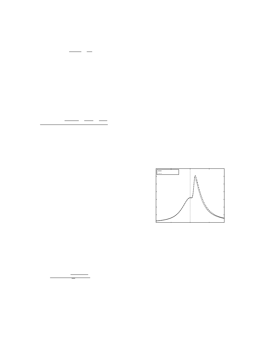
Figures 3 and 4 show that a single temperature threshold
fails to capture combustion phasing at different operating
conditions. This is due to the fact the initiation of the com-
bustion reaction depends not only on the temperature, but
also the concentration of species present in-cylinder. This
dependence on both temperature and concentrations is es-
pecially important in the case of HCCI, where reinducted
exhaust species from the previous cycle both dilute and
heat the reactant species. While the dilution of reactants
decreases the likelihood of combustion, the reactant heat-
ing increases the likelihood of combustion. The interplay
of these two phenomena leads to a self-stabilizing effect,
which corresponds to experimental observations of HCCI
using VVA.

−50

0

50

0

10

20

30

40

50

60

70

Crankshaft

°

ATC

Pressure (bar)

experiment
temp. threshold

Figure 3:

Temperature Threshold Approach: IVO @ 25deg.,

EVC @ 165

3.2 Two Step Mechanism
In order to capture the effects of both concentration and
temperature on combustion timing, a more detailed, yet still
simple, approach to modeling the combustion kinetics was
developed. In this case the reaction rate expressions de-
pend directly on both concentration and temperature using
well-known Arrhenius-type relations. Consider the two-
step mechanism:

C

3

H

8

+ 3.5O

2

+ 18.8N

2

→ 3CO + 4H

2

O

+ 18.8N

2

(31)

CO

+ .5O

2

↔ CO

2

(32)

−50

0

50

0

10

20

30

40

50

60

70

Crankshaft

°

ATC

Pressure (bar)

experiment
temp. threshold

Figure 4:

Temperature Threshold Approach: IVO @ 45deg.,

EVC @ 185

The reaction rates for C

3

H

8

oxidation and CO oxidation are

given in [11] as:

w

C

3

H

8

= 4.83e

9

exp

−15098

T

[C

3

H

8

]

.1

[O

2

]

1

.65

(33)

w

CO

,ox

= 2.24e

12

exp

−20130

T

[CO][H

2

O

]

.5

[O

2

]

.25

−5e

8

exp

−20130

T

[CO

2

]

(34)

These Arrhenius-type relations are commonly used to
model reaction rates in combustion mechanisms. By inspec-
tion of equation 32, the other reaction rates follow as:

w

O

2

= 3.5w

C

3

H

8

+ .5w

CO

,ox

(35)

w

N

2

= 0

(36)

w

CO

2

= −w

CO

,ox

(37)

w

H

2

O

= −4w

C

3

H

8

(38)

w

CO

= −3w

C

3

H

8

+ w

CO

,ox

(39)

Note that in this approach there is no need to track any
threshold values.

Results for this approach (Figures 5

−50

0

50

0

10

20

30

40

50

60

70

Crankshaft

°

ATC

Pressure (bar)

experiment
2 step mechanism

Figure 5:

Two Step Mechanism Approach: IVO @ 25deg., EVC
@ 165

and 6) show good correlation with experiment with respect
to combustion phasing, pressure rise, pressure decay and
peak pressure. However, there is a discrepancy in pres-
sure around the onset of combustion. More detailed mech-
anisms, with more reactions and corresponding Arrhenius

−50

0

50

0

10

20

30

40

50

60

70

Crankshaft

°

ATC

Pressure (bar)

experiment
2 step mechanism

Figure 6:

Two Step Mechanism Approach: IVO @ 45deg., EVC
@ 185

reaction rate expressions can be implemented in a compa-
rable way as the simple two step mechanism and be ex-
pected to show better correlation with experiment. How-
ever, the goal here is to keep the overall model simple, while
still capturing the combustion phasing and overall behavior.
The two step approach accomplishes this fairly well. It is
also clear through comparison with the temperature thresh-
old approach that both concentration and temperature must
be considered when modeling combustion timing.

3.3 Integrated Global Arrhenius Rate Threshold
The conclusion that both temperature and concentration
should be included in a description of combustion initia-
tion motivated a new approach with elements from both
of the previous approaches. In this case the proposed rate
of reaction of the propane is the same as that used for the
temperature threshold approach. Additionally, the idea of
a threshold parameter to mark the onset of combustion was
also adopted from the temperature threshold approach. The
difference is that the threshold used is the integration of an
Arrhenius type reaction rate expression similar to those used
in the two step mechanism approach, instead of a temper-
ature. This integrated reaction rate,

R

RR, then takes the

form:

Z

RR

=

Z

θ

0

AT

n

exp

(E

a

/(RT ))[C

3

H

8

]

a

[O

2

]

b

d

θ

(40)

such that:

w

C

3

H

8

=











[C

3

H

8

]

i

V

i

˙

θ

exp

h

−((

θ

−

θ

init )−

¯

θ

)

2

σ

2

i

V

σ

√

2

π

R

RR ≥

R

RR

th

0

R

RR

<

R

RR

th











(41)

where the threshold value of the integrated reaction rate,

R

RR

th

, has a value which correlates experiment and model

at one operating condition. By inspection of equation 25 the
reaction rates of the other species can be deduced as:

w

O

2

= 3.5w

C

3

H

8

(42)

w

N

2

= 0

(43)

w

CO

2

= −3w

C

3

H

8

(44)

w

H

2

O

= −4w

C

3

H

8

(45)

Like the results for the two step model, the predicted com-

−50

0

50

0

10

20

30

40

50

60

70

Crankshaft

°

ATC

Pressure (bar)

experiment
Integrated Arrhenius rate threshold

Figure 7:

Integrated Arrhenius Rate Threshold Approach: IVO

@ 25deg., EVC @ 165

−50

0

50

0

10

20

30

40

50

60

70

Crankshaft

°

ATC

Pressure (bar)

experiment
Integrated Arrhenius rate threshold

Figure 8:

Integrated Arrhenius Rate Threshold Approach: IVO

@ 45deg., EVC @ 185

bustion phasing with the integrated rate threshold approach
correlated with experiment, as can be seen in Figures 7 and
8. Furthermore, the pressure near the onset of combustion
matched experiment much better than the two step model.
However, slight discrepancies in pressure rise, maximum
pressure and pressure decrease can be noted along the pres-
sure peak.

4 Conclusion

Three different modeling strategies were developed and
compared to experimental results.

The main difference

among the three approaches was how the chemical kinet-
ics were modeled. In the simplest approach the kinetics
were assumed initiated once a temperature threshold was
attained. Following the crossing of this threshold, the rate
of consumption of mass of propane was approximated as

a gaussian like function. This approach showed unsatis-
factory results with significant deviations from experiment.
These deviations were attributed to the fact that species con-
centrations where not used to describe the combustion initi-
ation threshold. The second approach implemented a simple
two step mechanism, with Arrhenius-type reaction rates for
the oxidation of propane and carbon monoxide. Although
this method predicted combustion phasing well, it was de-
sirable to find a simpler approach that would still reflect ex-
perimental results. This was achieved in the third approach
developed by taking elements of both the previous models.
The idea of modeling the combustion initiation via a thresh-
old parameter was done by tracking the integration of the
Arrhenius global reaction rate for propane. As was the case
for the temperature threshold case, this was followed by a
gaussian type function to model the reaction rate of fuel.
This approach also correlated well with experimental com-
bustion timing.

References

[1]

P.A. Caton, A.J. Simon, J.C. Gerdes, and C.F. Ed-

wards. Residual-effected homogeneous charge compression
ignition at low compression ratio using exhaust reinduction.
International Journal of Engine Research, 4(2), 2003.

[2]

M. Christensen, A. Hultqvist, and B. Johansson.

Demonstrating the multi-fuel capability of a homogeneous
charge compression ignition engine with variable compres-
sion ratio. SAE paper 1999-01-3679.

[3]

Scott B. Fiveland and Dennis N. Assanis. A quasi-

dimensional HCCI model for performance and emissions
studies. Ninth International Conference on Numerical Com-
bustion, Paper No. MS052.

[4]

N.B. Kaahaaina, A.J. Simon, P.A. Caton, and C.F.

Edwards.

Use of dynamic valving to achieve residual-

affected combustion. SAE paper 2001-01-0549.

[5]

S.C. Kong, C.D. Marriot, R.D. Reitz, and M. Chris-

tensen. Modeling and experiments of HCCI engine comb-
sution using detailed chemical kinetics with multidimen-
sional CFD. Combustion Science and Technology, 27:31–
43, 1981.

[6]

D. Law, D. Kemp, J. Allen, G. Kirkpatrick, and

T. Copland. Controlled combustion in an IC-engine with
a fully variable valve train. SAE paper 2001-01-0251.

[7]

Joel Martinez-Frias, Salvador M. Aceves, Daniel

Flowers, J. Ray Smith, and Robert Dibble. Hcci engine con-
trol by thermal management. SAE paper 2000-01-2869.

[8]

Roy Ogink and Valeri Golovitchev. Gasoline HCCI

modeling: An engine cycle simulation cosde with a multi-
zone combustion model. SAE paper 2002-01-1745.

[9]

A.G. Stefanopoulou, J.W. Grizzle, and J.S. Freuden-

berg. Joint air-fuel ratio and torque regulation using sec-
ondary cylinder air flow actuators. ASME Journal of Dy-
namic Systems, Measurement, and Control, 121(4):638–
647, 1999.

[10] P. Tunestal, J-O Olsson, and B. Johansson. HCCI op-

eration of a multi-cylinder engine. First Biennial Meeting
of the Scandinavian-Nordic Section of the Combustion In-
stitute, 2001.

[11] Charles K. Westbrook and Frederick L. Dryer. Sim-

plified reaction mechanisms for the oxidation of hydrocar-
bon fuels in flames. Combustion Science and Technology,
27:31–43, 1981.