Ronald Bewley, Time Series Forecasting

1. Decomposition of Time Series

While the focus of this book is on forecasting, it is necessary to understand the

nature of the time series being predicted and some of the key historical developments in

the subject. The notion that a time series can be decomposed into additive or

multiplicative components representing trends, long-term cycles, seasonality and random

fluctuations has been the mainstay of much of forecasting’s development. However, a

growing literature has emerged on the modelling of seasonality, led by Svend Hylleberg

and Philip Hans Frances, that has challenged this approach.

The detrending of time series has similarly been the subject of much research and

development, from the early simple averaging techniques, through smoothing models and,

more recently, so-called smoothing filters.

Whether or not one accepts the classical decomposition of time series, or the joint

modelling of all the components, there is little doubt that the more advanced forecasting

methods considered in this book are sufficiently complex without joint modelling to

warrant their investigation assuming that data have been suitable transformed before the

forecasting analysis has commenced. Of course, this point of view does not preclude

awareness of the main criticisms of this approach nor some simple tests to detect the

possible importance of ignoring even more sophisticated approaches.

1.1 The Nature of Time Series

1.1.1 Definitions

A time series is a sequence of observations measured over time (usually at equally

spaced intervals; e.g. weekly, monthly, or annually) and can take the form of, say, Gross

Domestic Product each quarter; annual rainfall; or the daily Stock Market Index.

Within the definition of time series, two distinctions can be made. First, a time

series is said to be deterministic or stochastic depending on whether or not the series is

perfectly predictable. In econometrics, data are stochastic in that there is an inherent

random component which cannot be predicted, although it is sometimes assumed that there

is an underlying deterministic component buried in unpredictable ‘noise’. For example, in

the simple regression equation

y

t

=

α

+

β

x

t

+ u

t

,

the variable x is fixed, or given, as are the parameters

α

and

β

. Thus (

α

+

β

x

t

) is a

UNSW, July 2000 Draft, Decomposition of Time Series

deterministic component buried in noise, denoted by u

t

, the disturbance term.

A second distinction can be made between continuous and discrete time series. A

continuous series can, in theory, be measured at any point in time (e.g. there is always a

temperature, whether or not one chooses to measure it) although the measuring device

(e.g. a thermometer) may only permit the series to be collected with a finite interval (e.g.

every 1/100th second) giving rise to a particular type of discrete process known as a

sampled series. On the other hand, a discrete process can only be observed at given points

in time. The usual distinction between continuous and discrete series results from the

difference between stocks and flows. For example, the stock of wealth is continuous but

income, the flow, only exists on, say, a weekly, monthly or annual basis. Note the two

statements “My wealth is $10,000” and “My income is $1,000”. The former statement

might be true but the latter is meaningless without reference to the time period.

1.1.2 Time Series Versus Causal Modelling

Typically in econometrics, causal models are preferred to simple extrapolative

techniques. In causal models, the econometrician specifies some behavioural relationship

and estimates the parameters using regression techniques. Given such an estimated

relationship, past movements in the series can be explained, and future movements in the

series predicted, once assumptions are made about the behaviour of the independent

variables in the model. However, there are many cases when one cannot, or one prefers

not to, build a causal model:

1)

insufficient is known about behavioural relationships.

2)

lack of, or conflicting, theory.

3)

insufficient data on explanatory variables.

4)

a causal model is too expensive to build.

5)

expertise unavailable.

6)

causal model is not cost effective.

7)

time series models may be more accurate.

Time series models are not without some theoretical justification and there is little

doubt the popularity of time series analysis led econometricians to consider a wider class

of dynamic specification in the more conventional approach. Furthermore, there are some

2

Ronald Bewley, Time Series Forecasting

direct benefits to employing time series modelling procedures:

1)

limited computer storage needed for some time series models.

2)

some

time

series

models

are

automatic

in

that

user

intervention is not required to update the forecasts each

period.

3)

some time series models are evolutionary in that the

coefficients and, hence, the trends adapt as new information

is received.

4)

some time series models can be ‘put back on track’

automatically after a poor forecast.

1.1.3 Classical Decomposition of Time Series

In the classical decomposition of a time series, any series is thought to comprise

four components: trend, cycle, seasonal and random.

Trend

in this context trend does not imply a monotonically

increasing or decreasing series but simply the lack of a

constant mean. That is, different sections of a series may

have quite different sample means indicating that the

population mean is time dependent.

Cycle

refers to patterns, or waves, in the data that are repeated after

approximately

equal

intervals

with

approximately

equal

intensity.

For

example,

some

economists

believe

that

‘business cycles’ repeat themselves every four or five years

but occasionally a recession may last considerably longer

than the usual 1-2 years.

Seasonal

refers to a cycle of one year duration. There may, however,

be one or more peaks in a year and, in high frequency data, a

‘year’ may refer to a week and daily variation corresponds to

‘seasonal’ behaviour.

Random

refers to (unpredictable) variation not covered by the above.

3

UNSW, July 2000 Draft, Decomposition of Time Series

By way of example, consider the decomposition of the Australian monthly current

account series:-

Trend - is Australia on a downhill track? This raises the important question of when a

long-term cycle becomes a trend. For this reason, trend and cycle are often amalgamated

into one ‘trend’ component.

Cycle - (business cycle) The economy finds it hard to meet demand at the peak of a

business cycle and so imports more (‘The economy overheats’).

Seasonality - imports of clothing are seasonal, as are agricultural exports and foreign aid

payments.

Random - whether a 747 jumbo jet is imported on September 1 or August 30 makes a

large difference to the behaviour of the monthly account.

1.1.4 Trend Estimation

It is usually optimal to jointly estimate the trend and other time series components.

However, this approach usually requires a formal econometric model to be specified.

Alternatively, it can be useful to consider aggregating observations over time to

smooth data so as to highlight any trend. In particular, monthly data may be aggregated to

quarterly data and this will have a smoothing effect as random variation is averaged over

successive periods. However, such ‘temporal aggregation’ reduces the data set to, say, one

third of the original set when monthly data are aggregated into quarterly data. Seasonality

is typically removed or reduced by temporal aggregation.

Although temporal aggregation smooths data, there are certain negative aspects. For

example, when monthly data are aggregated into annual data, one must wait a full year or

more before a new observation is collected. Consequently new trends are detected much

later than with monthly data.

It is important in time series analysis to appreciate that a mean does not always

exist. While a sample mean can always be computed, inferences about a population mean

require that such a mean exists. For example, consider a time trend model

y

t

=

α

+

β

t + u

t

In such cases, no (constant) mean exists. One can, however, consider the concept of a

local mean in some neighbourhood. The mechanism for evolution of the local mean is the

4

Ronald Bewley, Time Series Forecasting

trend.

Consider the following averaging processes:-

Take the mean of adjacent pairs

(y

1

+ y

2

)/2 , (y

3

+ y

4

)/2 , ...

Clearly this averaging process reduces the size of the data set. However, it is a simple

matter to consider overlapping averages:

(y

1

+ y

2

)/2 , (y

2

+ y

3

)/2 , (y

3

+ y

4

)/2 , ...

and this variant only loses one observation while smoothing the series. Note, however, that

the average of observations 1 and 2 is aligned with time t = 1½ which has no

interpretation with discrete series. If the m successive observations are averaged and m is

odd, there is no problem:

(y

t-1

+ y

t

+ y

t+1

)/3 = m

t

(1.1.1)

is centred at time t and m

t

is known as a 3-point moving average.

Example Consider the data in column 1 of Table 1.1. Each element of column 2 is the

sum of three consecutive observations as defined by equation (1). The third column is the

second divided by three, i.e. the MA(3) process but note that there is no estimate of the

MA(3) corresponding to the first or last observation.

Table 1.1: Computation of an MA(3) Process

y

t

Sum

m

t

10

?

12

33

11

11

30

10

7

24

8

6

15

5

2

?

It is important to note that the longer the MA, that is the number of observations

being averaged, the smoother is the series. An MA(m) removes a cycle of period m but an

5

UNSW, July 2000 Draft, Decomposition of Time Series

MA(m+1) reduces, but does not remove a cycle of period m. For example, with monthly

data, a twelve period MA removes seasonality but a thirteen-period MA has two months

of January in the July average etc. but a less pronounced degree of seasonality exists in

the smoothed data than in the raw data.

Because many interesting cycles are of even length (12 months, 4 quarters, etc.), it

is useful to consider ‘convolutions’ of MA processes in order to ‘centre’ the MA

smoothed data. Consider an MA(3) of an MA(3); that is, the smoothed data are again

smoothed in the same manner.

The first three columns in Table 1.2 have been constructed on the same basis as

the corresponding columns in Table 1.1. Each element in the fourth column is the centred

sum of three consecutive elements of column (3) and the final column has been derived by

dividing the fourth column by 3.

Table 1.2: Computation of an MA(3*3) Process

y

t

Sum

MA(3)

Sum

MA(3*3)

10

?

?

?

12

33

11

?

?

11

30

10

29

9

7

24

8

23

7

6

15

5

?

?

2

?

?

?

The complete calculation for the third element of the smoothed series (9 ) is

derived from

9

= 11 + 10 + 8 = (10+12+11)/3 + (12+11+7)/3 + (11+7+6)/3

3

3

= (1/9) [1(10) + 2(12) + 3(11) + 2(7) + 1(6)]

=

(1/9)

y

1

+

(2/9)

y

2

+

(3/9)

y

3

+

(2/9

)y

4

+

(1/9)

y

5

6

Ronald Bewley, Time Series Forecasting

and it follows that the fourth element of the smoothed series (7 ) is given by

7

=

(1/9)

y

2

+

(2/9)

y

3

+

(3/9)

y

4

+

(2/9

)y

5

+

(1/9)

y

6

The sequence {1/9, 2/9, 3/9, 2/9, 1/9} defines the weights of the MA process or

filter since it filters out the noise in a series. Note that an MA(3*3) has 5 weights, the

weights are symmetric about the central observation, the maximum weight is at the centre,

and the weights sum to unity. A 3 * 3 MA is a centre-weighted MA. In general, an

MA(m*m), with m odd, has weights {1/m

2

, 2/m

2

, ...,m/m

2

, ...1/m

2

} and there are (2m-1)

weights. ‘Even’ MA processes are not centre-weighted but two even MA processes are

centred when convoluted.

When choosing an MA process, it should be recalled that a longer length produces

less randomness but more data are lost and the MA estimate of the trend is slower to react

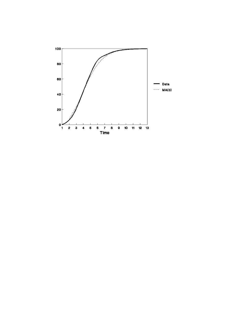
to any new trend in the data. For example, consider smoothing a growth curve. An

example is presented in Figure 1. Clearly, the trend estimate MA(3) under-predicts a

decreasing trend and over-predicts an increasing trend.

Because there is a lag of (m-1)/2 periods between the latest observation of the raw

series and the latest smoothed estimate, a one-sided MA is sometimes used. To be useful,

the weights of a one-sided filter need to decline, and sum to unity, as in the following

example

m

t

= 0.6 y

t

+ 0.3 y

t-1

+ 0.1 y

t-2

Optimal choices for the weights in such an MA process are considered in Section 1.2.

1.1.5 Seasonality

Seasonality is a pattern in the data which tends to replicate itself approximately in

successive years. If it were completely regular and, hence, deterministic in nature, it would

not present a problem. It is the randomness in the timing of the effects and the strength of

the variation that hampers investigation of seasonal data. Many methods have been

developed to cope with the problem and these fall into one of two categories: some

methods have been suggested which remove, or filter out, the seasonal effect from the data

before analysis while others are designed to deal jointly with the analysis and seasonality

at the modelling stage. The most well known from the former category is the classical

decomposition of time series using centre weighted moving averages.

7

UNSW, July 2000 Draft, Decomposition of Time Series

Figure 1.1: Smoothing a Growth Curve

Consider that a time series, y

t

, can be written as the sum of three components: trend (m

t

),

seasonal (s

t

), and irregular (r

t

)

y

t

= m

t

+ s

t

+ r

t

(1.2)

or, in multiplicative fashion:

y

t

= m

t

x s

t

x r

t

(1.3)

Clearly, a logarithmic transformation of (1.3) can be written in the form of (1.2) and the

choice of (1.2) or (1.3) depends on whether the seasonal component is constant over time

or is amplified by the trend. In many cases where there is a strong trend, (1.3) will be

appropriate, but there are cases when neither (1.2) nor (1.3) are adequate.

In order to isolate the seasonal component, some estimate of the trend is required.

A simple method of estimating the underlying trend is given by locally averaging the data

in a (centre-weighted) moving average as discussed earlier.

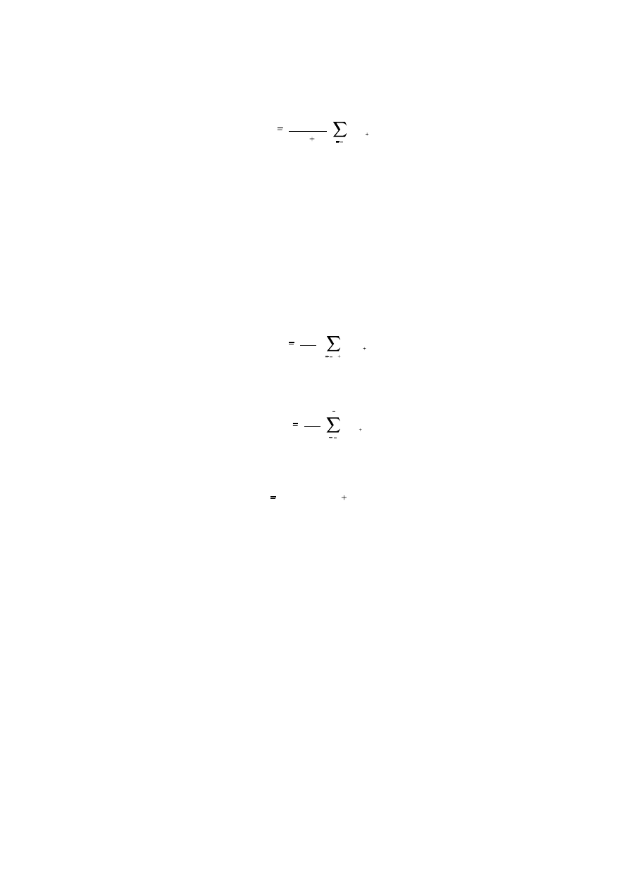
Specifically, consider that there are 2n + 1 periods (i.e. an odd number) in a year.

The averaging operator

8

Ronald Bewley, Time Series Forecasting

(1.1.4)

m

t

1

(2n 1)

n

i

n

y

t i

includes exactly one occurrence of each period within a year and so, m

t

can be considered

nonseasonal. If the number of periods in a year is even, the procedure is slightly more

complicated. The problem arises because the ‘centre-weighting’ principle would leave an

estimate of the trend corresponding to t+½ which is not meaningful with discrete data. In

such cases, the successive values of the trend are themselves averaged as follows. Let

there be 2n periods (i.e. an even number) in a year and define

and

(1.1.5)

m

(1)

t

1

2n

n

i

n 1

y

t i

with

(1.1.6)

m

(2)

t

1

2n

n 1

i

n

y

t i

Given that the trend can be isolated, the seasonal plus irregular component can be

(1.1.7)

m

t

(1/2) [m

(1)

t

m

(2)

t

]

extracted as

s

t

+ r

t

= y

t

- m

t

(1.1.8)

or

s

t

x r

t

= y

t

/m

t

(1.1.9)

Since r

t

is assumed to be noise, the seasonal component is found by averaging

either (1.1.8) or (1.1.9) for all observations corresponding to the same period in each year.

The steps of the calculations are given in Table 1.3 for Australian Retail Sales in

constant 1984/5 dollars. The second column displays the unadjusted quarterly data and the

third column presents the sum of four consecutive observations of the y

t

data (which is a

multiple of m

t

(1)

given by equation (1.1.5). The fourth column contains the sum of two

adjacent terms of column (3) while the fifth column contains the moving average trend,

9

UNSW, July 2000 Draft, Decomposition of Time Series

m

t

. In column (6), the unadjusted data are divided by the trend to produce a ‘raw’ estimate

of the seasonal times the irregular component as in equation (1.1.9).

Table 1.3: Seasonal Adjustment of Retail Sales Data

Date

y

t

Sum(4)

Sum(2)

m

t

(y

t

/m

t

)

s

t

(y

t

/s

t

)

ABS

(1)

(2)

(3)

(4)

(5)

(6)

(7)

(8)

(9)

82-II

13423

0.96

13928

13773

82-III

13129

0.97

13598

13599

82-IV

15399

54915

109540

13693

1.12

1.13

13631

13621

83-I

12964

54625

109394

13674

0.95

0.94

13782

13898

83-II

13134

54768

109734

13717

0.96

0.96

13627

13518

83-III

13272

54966

109985

13748

0.97

0.97

13746

13725

83-IV

15596

55020

110315

13789

1.13

1.13

13805

13793

84-I

13018

55295

110623

13828

0.94

0.94

13839

13742

84-II

13409

55328

110933

13867

0.97

0.96

13913

13824

84-III

13304

55605

111559

13945

0.95

0.97

13780

13921

84-IV

15874

55954

112497

14062

1.13

1.13

14051

14088

85-I

13367

56543

113827

14228

0.94

0.94

14210

14254

85-II

13999

57284

115345

14418

0.97

0.96

14525

14455

85-III

14045

58061

116353

14544

0.97

0.97

14547

14596

85-IV

16650

58292

116769

14596

1.14

1.13

14738

14706

86-I

13598

58477

117037

14630

0.93

0.94

14456

14589

86-II

14183

58560

116851

14606

0.97

0.96

14716

14617

86-III

14129

58291

116496

14562

0.97

0.97

14634

14633

86-IV

16381

58205

116249

14531

1.13

1.13

14500

14479

87-I

13513

58044

116191

14524

0.93

0.94

14365

14416

87-II

14022

58147

116651

14581

0.96

0.96

14549

14508

87-III

14232

58504

117499

14687

0.97

0.97

14741

14761

87-IV

16737

58995

118134

14767

1.13

1.13

14815

14757

88-I

14005

59139

118250

14781

0.95

0.94

14888

14757

88-II

14166

59111

118380

14797

0.96

0.96

14698

14659

88-III

14204

59269

118782

14848

0.96

0.97

14712

14668

88-IV

16895

59513

119579

14947

1.13

1.13

14955

14910

89-I

14248

60067

120785

15098

0.94

0.94

15147

15216

89-II

14720

60719

121904

15238

0.97

0.96

15273

15196

89-III

14856

61185

122707

15338

0.97

0.97

15387

15397

89-IV

17362

61522

123198

15400

1.13

1.13

15368

15478

90-I

14585

61676

123295

15412

0.95

0.94

15505

15413

90-II

14874

61619

122990

15374

0.97

0.96

15433

15393

90-III

14798

61372

122443

15305

0.97

0.97

15328

15456

90-IV

17115

61071

121826

15228

1.12

1.13

15149

15209

91-I

14285

60755

121622

15203

0.94

0.94

15186

15211

91-II

14557

60867

121937

15242

0.96

0.96

15105

15048

91-III

14910

61070

122610

15326

0.97

0.97

15444

15474

91-IV

17318

61540

1.13

15329

15356

92-I

14755

0.94

15685

15531

The next step is to average certain elements in column (6) and this is facilitated by

10

Ronald Bewley, Time Series Forecasting

organising the data as in Table 1.4. That is, the estimates in column (6) of Table 1.3 are

arranged by quarter and the columns of Table 1.4 are averaged to produce a unique

seasonal multiplier for each quarter. These four estimates are then repeated in column (7)

which, when divided into column (2) produces the seasonally adjusted series in column

(8). The Australian Bureau of Statistics seasonally adjusted data are presented in the final

column of Table 1.3 for comparison. An additive seasonal model would differ from that

described only in that the divisions in columns (6) and (8) become subtractions.

It can be computed from Table 1.4 that the average of the four seasonal ratios is

very close to one, as is desirable. If it transpires that the mean is not one (or zero for the

additive model), it is important to adjust the four estimates so that the mean is one.

Otherwise, there will be a bias in the level of the adjusted series.

Table 1.4: Forming the Seasonal Ratios

Year

Quarter

I

II

III

IV

1982

1.125

1983

0.948

0.957

0.965

1.131

1984

0.941

0.967

0.954

1.129

1985

0.939

0.971

0.966

1.141

1986

0.930

0.971

0.970

1.127

1987

0.930

0.962

0.969

1.133

1988

0.947

0.957

0.957

1.130

1989

0.944

0.966

0.969

1.127

1990

0.946

0.967

0.967

1.124

1991

0.940 0.955

0.973

Average

0.941

0.964

0.965

1.130

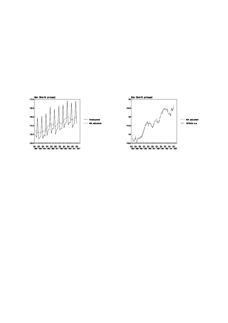
The impact of the seasonal adjustment procedure can be judged in the following

graphical analysis. In Figure 1.2(a), the marked seasonal pattern in retail sales makes it

extremely difficult to judge whether a quarter-to-quarter change is due only to seasonal

11

UNSW, July 2000 Draft, Decomposition of Time Series

effects or if it is of more substance. The adjusted data in the Figure, having separated out

the seasonal effects, makes it simpler to notice changes in trend values. In the companion

Figure 1.2(b), the series as seasonally adjusted by the Australian Bureau of Statistics is

compared to that derived in Table 1.3.

Figure 1.2: Seasonal Adjustment of Retail Sales

1.2(a) Adjusted and Unadjusted Data

1.2(b) Alternative Procedures

It can be noted from Figure 1.2(b) that the additional gains from employing the

more complicated ABS procedures are not great. However, it should be emphasised that, if

quarter-to-quarter changes are under consideration, the differences between the two

methods would be magnified.

Since the adjusted series contains the irregular component, it is necessarily more

volatile than the trend series, m

t

, as shown in Figure 1.2(a). In some sense, the trend series

gives a clearer picture of longer-term swings in the data but it should be noted that, in the

case of quarterly data, there are no trend estimates for the first and last two quarters.

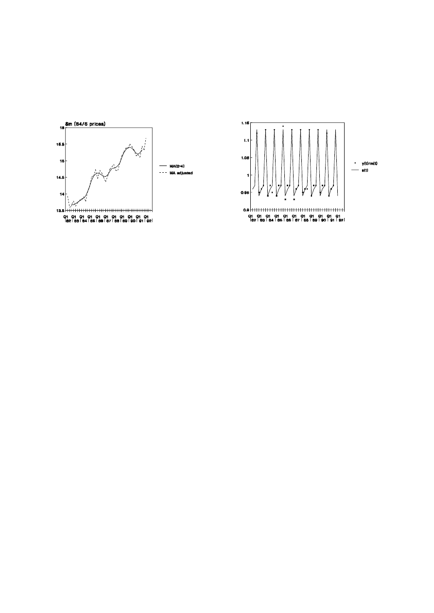
A fundamental assumption of the seasonal adjustment procedure is that the

seasonal effect is constant over time. By comparing the series of seasonal and irregular

component [column (6), Table 1.3] with the average effects [column (7), Table 1.3], it can

be noted that the assumption is reasonably valid. If, however, the amplitude of the raw

seasonal coefficients had been increasing or decreasing, assumptions other than that of

multiplicative effects would need to have been considered.

12

Ronald Bewley, Time Series Forecasting

Figure 1.3: Validity of Adjustment Procedure

1.3(a) Seasonally Adjusted Data and

3(b) Regularity of Seasonal Component

Moving Average Trends

1.2 Smoothing Methods

Exponential smoothing, Holt’s method and Winters’ Method, collectively known as

smoothing methods originated as simple, automatic forecasting techniques. They are

automatic in the sense that coefficients are often imposed rather than estimated, forecasts

are typically updated without re-estimation, and only limited amounts of data need to be

stored. However, there is no reason why the parameters are not estimated. Despite the

apparent simplicity of these methods and the availability of more sophisticated techniques,

smoothing methods remain popular in the business forecasting environment.

It will be shown that Holt’s method is a generalisation of exponential smoothing

that allows for a trend in the forecasts and Winter’s method is a further generalisation

which accommodates an evolving seasonal pattern.

1.2.1 Averages

Assume that there is no trend nor seasonality in a data series and that y

t

is

completely random and normally distributed as N(0,

σ

2

). The optimal model is, therefore,

y

t

= µ +

ε

t

(1.2.1)

E(

ε

t

) = 0 ; E(

ε

2

t

) =

σ

2

; E(

ε

t

ε

s

) = 0 if s

≠

t, hence the mean of y

t

is µ and there is a zero

correlation between successive values of y

t

. To estimate (1.2.1), consider a formal least

squares solution. Let

13

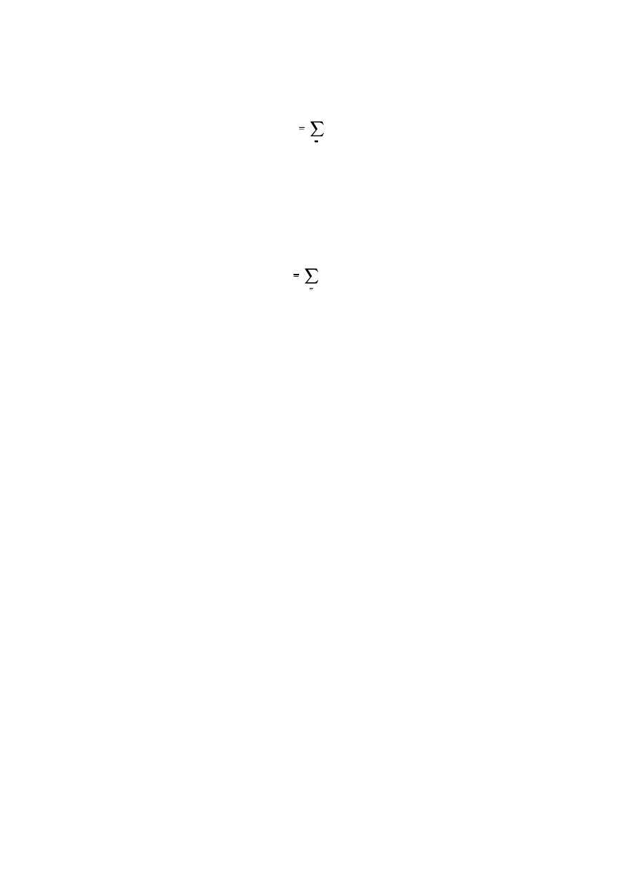
UNSW, July 2000 Draft, Decomposition of Time Series

where e

t

is the regression residual

S

T

t 1

e

2

t

e

t

= y

t

- m

and m is the estimate of µ. In least squares, S is minimised with respect to m and it can

easily be shown that

That is, the mean is the best forecast for all future time.

m

T

t 1

y

t

/T

yˆ

T

(k) = m

where k is the lead time of the forecast and T is the forecast origin. That is, yˆ

T

(k) is the

forecast of y

T+k

made at time t.

As new data becomes available: y

T+1

, ... ,y

T+n

, forecast errors can be defined:

e

T

(1) = y

T+1

- yˆ

T

(1)

(one-step forecast error)

e

T

(2) = y

T+2

- yˆ

T

(2)

(two-step forecast error)

.
.
.

e

T

(k) = y

T+k

- yˆ

T

(k)

(k-step forecast error)

1.2.2 Shifting Mean

Often in business and economics, it can be noted that a time series tends to shift,

or ‘float’, over time so that different sections of the series appear to have different levels

or means. In such cases it does not make sense to define the mean to be fixed over time

and so more emphasis might be placed on recent data when forecasting. This distinction

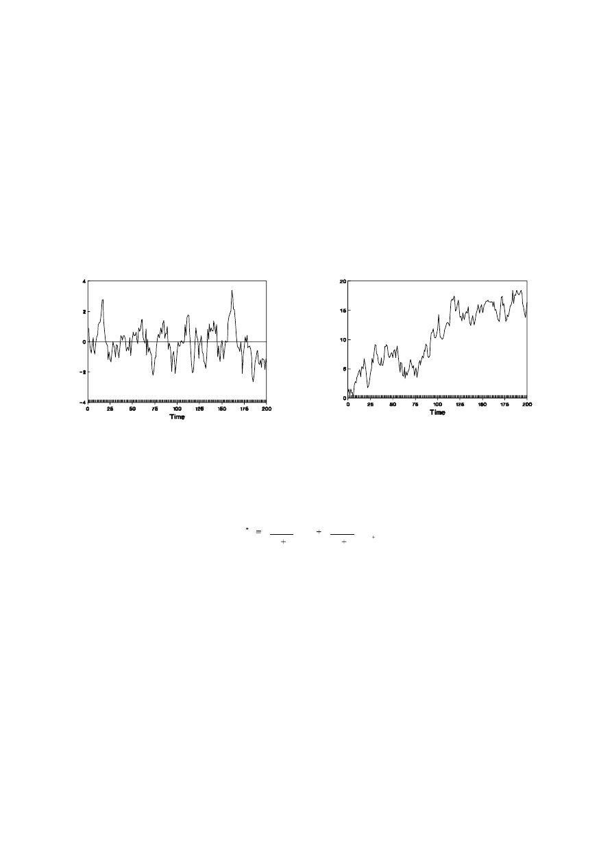
between series which frequently cross the mean [Figure 1.4(a)], that is exhibit mean

reversion and those that tend evolve over time [Figure 1.4(b)] is important for time series

analysis and will be defined more rigorously in subsequent chapters.

The simplest solution when dealing with series that evolve as in Figure 1.4(b) is to

average only the last T observations [in an MA(T) process] but this is usually

unsatisfactory for forecasting purposes. Unequal weights, such as given in

14

Ronald Bewley, Time Series Forecasting

m

t

= 0.4 y

t

+ 0.3 y

t-1

+ 0.2 y

t-2

+ 0.1 y

t-3

partially address this issue but these weights are somewhat arbitrary. One particular, and

extremely popular, variant of the unequal weight case is given by exponential smoothing

to be introduced later in this chapter. First, however, consider how an MA(T) process is

updated as new data becomes available.

Figure 1.4: Existence of Means

1.4(a) Mean Reversion

1.4(b) Shifting Mean

If the mean is assumed constant, but its estimate, m, is updated as new data

becomes available, the estimate with T observations, m

*

is linked to the old mean

[Appendix 1A] by

It follows from equation (1.2.2) that new data, y

T+1

, has decreasing importance

(1.2.2)

m













T

T 1

m













1

T 1

y

T 1

since (T+1)

-1

→

0 as T

→ ∞

. It can also be noted that it is only necessary to store two

numbers, m and T, not the whole data set, in order to update the mean when y

T+1

is

released.

If the above relationship is adapted for the T-period moving average situation, that

is one observation is dropped from the earliest period when the new data point is added, it

is shown in Appendix 1B that

15

UNSW, July 2000 Draft, Decomposition of Time Series

and it follows that T observations need to be stored if the process is to be updated.

m

m

(1/T) y

T 1

(1/T) y

1

1.2.3 Discounted Least Squares

Instead of considering minimising the residual sum of squares

as is done in standard regression analysis, consider a discounted least squares approach

S

T

t 1

e

2

t

T 1

i 0

y

T i

m

2

where

λ

is a fixed constant between zero and one. What was a constant, m, in standard

S

∞

i 0

λ

i

y

T i

m

T

2

regression is no longer a constant but m

T

, which depends on y

1

,...,y

T

. On setting dS

*

/dm

T

= 0, and rearranging, an updating formula can be derived for the discounted least squares

estimate of m using data up to and including time T, m

T

:

m

T+1

=

λ

m

T

+ (1-

λ

)y

T+1

(1.2.3)

That is, the new forecast m

T+1

is a weighted average of the old forecast m

T

and the new

observation y

T+1

. Since the basic model is that of representing the data by its local mean,

the forecast for all future time is m

T+1

until new information arrives.

Clearly

λ ≤

1 for the sum S

*

to be defined. If

λ

= 0, the old mean is ignored

and, m

T

= y

T

. If

λ

= 1, the new observation is ignored and m never changes, regardless of

the new data; m

T

= m

T-1

. Typically,

λ

> 0.

On noting that m

T

is the forecast of y

T+1

, equation (1.2.3) can be rewritten in terms

of the forecasts yˆ

T

(1), etc., and, by defining

λ

= (1-

α

):

yˆ

T

(1) = (1-

α

)yˆF

T-1

(1) +

α

y

T

(1.2.4)

and, after more algebra

yˆ

T

(1) = (1-

α

)

k+1

yˆ

T-k-1

(1) +

α

[y

T

+ (1-

α

)y

T-1

+ (1-

α

)

2

y

T-2

... + (1-

α

)

k

y

T-k

]

which demonstrates that the weights on y

T-i

are geometrically declining. The geometrically

declining pattern, which in the limit, as the time interval between successive observations

16

Ronald Bewley, Time Series Forecasting

approaches zero, is exponential, gives this method its name, Exponentially Weighted

Moving Average (EWMA) or Exponential Smoothing.

On substituting the definition of the one-step forecast error into (1.2.4), it can be

shown that

yˆ

T

(1) = yˆ

T-1

(1) +

α

e

T-1

(1)

(1.2.5)

That is, the EWMA is an error learning process; the old forecast is updated by some

proportion (

α

) of the old forecast error.

In order to make the EWMA operational, it is necessary to provide starting values.

That is, the forecast of the first observation, yˆ

0

(1), and a value for

α

. Since yˆ

0

(1) is a local

mean, this initial value is often taken to be the average of, say, the first three observations.

Note that if one has a lack of confidence about the initial value, a fairly high value

of

α

, say 0.5, can be chosen for, say, the first 20 observations so that new information is

weighted highly, for a ‘settling-in period’. The value of

α

can then be lowered to say 0.2

for forecasting purposes.

It is unusual to estimate

α

, as this defeats the simplicity of the approach, but it is

not uncommon for a grid search to be used to determine the sensitivity of the forecasts to

different values of

α

. For example, five or six different values of

α

are used and that

which produces the best fit over the sample is selected.

The EWMA is suboptimal when there is a linear trend in the data. Indeed, it can

be shown that EWMA forecasts lag behind the actual data with the bias being greater, the

smaller is the value of

α

. Holt’s method corrects for this bias and Winter’s method allows

for both trends and seasonality.

1.2.4 Share Price Index

The EWMA is best suited to series which exhibit the properties of time series such

as the Australian share price index. Monthly data from 1958 (Jan) to 1992 (April) were

used with the microTSP estimation procedure for exponential smoothing. The optimal

estimate for

α

was 0.99 but, in Figure 1.5, the forecasting properties of series with

α

= 0.1

and

α

= 0.5 are compared.

Clearly, when

α

is small, the EWMA forecasts are slow to react to new trends,

such as those exhibited in the late 1980’s boom. On the other hand, the higher levels of

α

17

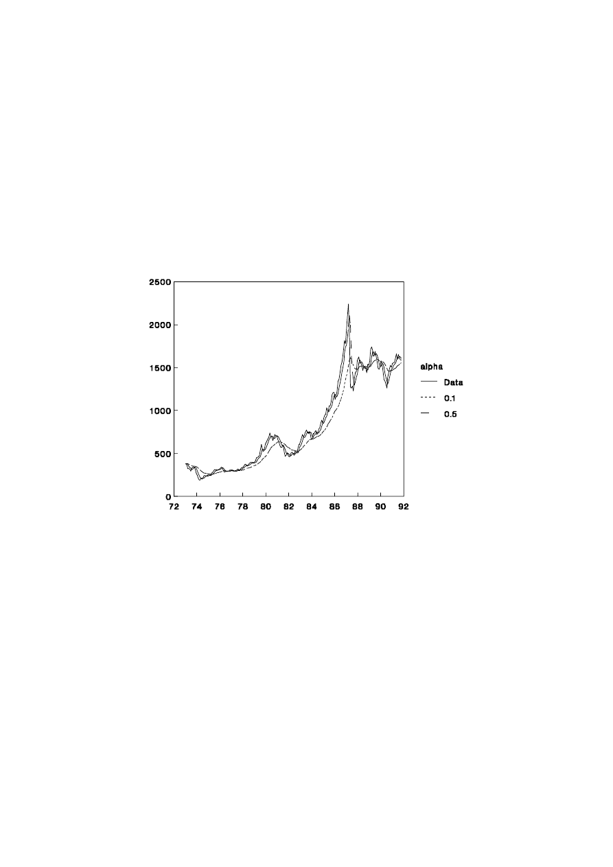
UNSW, July 2000 Draft, Decomposition of Time Series

imply that the forecasts over-react when an outlier occurs such as in September 1987

before the stock market crash.

The main problem with the EWMA forecast is that the best forecast for all future

time is the same as that for the next period. While this might be optimal for particular

series, the method is not sufficiently general for the many and varied applications of

forecasting techniques.

Figure 1.5: Share Price Index and EWMA Forecasts

1.2.5 Data Generating Process

The exponential smoothing method has a formal regression equation interpretation.

Recall the EWMA (1.2.5)

yˆ

t

(1) = yˆ

t-1

(1) +

α

e

t-1

(1)

(1.2.6)

and the definition of the one step forecast error

e

t-1

(1) = y

t

- yˆ

t-1

(1)

(1.2.7)

Now consider the data generating process

∆

y

t

= a

t

-

θ

a

t-1

(1.2.8)

where a

t

is N(0,

σ

2

) and i.i.d. [an expression which stands for independent and identically

18

Ronald Bewley, Time Series Forecasting

distributed; independent implies successive values of a

t

are not correlated and identical

implies that all a

t

have the same mean, variance and other distributional characteristics].

That is, a

t

has the same properties as the disturbance in a standard regression equation; in

time series analysis the term white noise is usually applied to such an error process.

∆

is

the first-difference operator such that

∆

y

t

= y

t

- y

t-1

. Equation (1.2.8), therefore, states that

the change in y

t

is not totally random unless

θ

= 0, but is related to the ‘shock’ or

disturbance term in the previous period. The forecasts from this model are equivalent to

those from the error-learning EWMA model.

Equation (1.2.8) can be written as

y

t

= y

t-1

+ a

t

-

θ

a

t-1

which, one period later, becomes

y

t+1

= y

t

+ a

t+1

-

θ

a

t

(1.2.9)

In order to produce a forecast from (1.2.9) for period t+1 it is necessary to replace

the right hand side of (1.2.9) by the best forecast of each term using information up to and

including that available at time t. This is known as taking conditional expectations (at time

t) of (1.2.9).

(i)

At time t the ‘best guess’ of a

t+1

is zero since it is, by definition,

unpredictable. Thus, E

t

(a

t+1

) = 0.

(ii)

At time t, a

t

has already occurred and the best guess of this term is the

forecast error e

t

. A more rigorous approach could, indeed, prove that the

disturbances that drive the process are the one-step forecast errors. Thus,

E

t

(a

t

) = e

t-1

(1).

(iii)

At time t, y

t

has occurred and is, therefore, known with certainty. Thus,

E

t

(y

t

) = y

t

.

(iv)

At time t, y

t+1

is unknown and so its conditional expectation is the forecast.

Thus E

t

(y

t+1

) = yˆ

t

(1).

Using the results of (i) - (iv), the conditional expectation of equation (1.2.9) is

yˆ

t

(1) = y

t

-

θ

e

t-1

(1)

(1.2.10)

and, substituting (1.2.7) into (1.2.10),

yˆ

t

(1) = yˆ

t-1

(1) +

α

e

t-1

(1)

(1.2.11)

where

α

= (1-

θ

). Clearly, equation (11) is of the same form as the EWMA in equation

19

UNSW, July 2000 Draft, Decomposition of Time Series

(1.2.6).

The right hand side of (1.2.8), a

t

-

θ

a

t-1

, is known as an MA (moving average)

process (of order 1) but it should be noted that the ‘weights’ do not sum to one as they

must in the similarly named MA smoothing methods.

Although the MA process given in equation (1.2.7) has no direct, intuitive

interpretation, the fact that it produces forecasts that are identically equal to an error

learning process motivates its use in business forecasting.

1.2.6 Holt’s Method

Holt’s method assumes that the data can be best summarised as having a local

mean, m

T

, as with the EWMA model, and a local (linear) trend,

τ

T

. Thus the forecasts

made at time T can be expressed as

yˆ

T

(k) = m

T

+ k

τ

T

(1.2.12)

Because of the importance of the trend in longer term forecasts, together with the

sensitivity of the estimate,

τ

T

is usual smoothed with a much smaller smoothing constant,

β

:

m

T

=

α

y

T

+ (1-

α

) (m

T-1

+

τ

T-1

)

(1.2.13)

τ

T

=

β

(m

T

- m

T-1

) + (1-

β

)

τ

T-1

(1.2.14)

It follows from (1.2.12) that the best forecast of y

T

is (m

T-1

+

τ

T-1

) so that the new

local level in (1.2.13) is a weighted average of the two, as in the EWMA model. The most

recent estimate of the trend is (m

T

- m

T-1

) so that the new estimate,

τ

T

, is a (differently)

weighted average of the two.

Holt’s method can also be written in terms of the forecast error

m

T

= (m

T-1

+

τ

T-1

) +

α

e

T

(1.2.15)

τ

T

=

τ

T-1

+

αβ

e

T

(1.2.16)

Since both

α

and

β

are between zero and one, the weight given to updating the trend is

less than that given to the level.

1.2.7 Winter’s Method and Seasonality

Further modifications can be made to the EWMA model to allow for seasonality in

either additive or multiplicative form. Winter’s method, described in Appendix 1C, allows

20

Ronald Bewley, Time Series Forecasting

for evolving seasonal patterns but its use in practice is somewhat limited and will not be

pursued here. A simpler, pragmatic approach when dealing with seasonal data is to first

use the seasonal adjustment procedure of Section 1.1 and then use the EWMA or Holt’s

method to make seasonally adjusted forecasts. If it is desired that the forecasts should

exhibit the same seasonal pattern as the data, the seasonal factors can be multiplied or

added to the forecasts

1.2.8 Henderson’s Trend Method

Many time series published by the Australian Bureau of Statistics are also

published in trend form. The method of deriving the trend is no more than a simple

moving average method with two modifications over that presented in Section 1.1. The

weights are derived from a more complicated process and these weights are published in

ABS Cat No. 1316.0, Estimates of “Trend”. Secondly, one-sided moving averages are used

for more recent data.

In each case, the ‘Henderson’ method requires the data to be first seasonally

adjusted, then, depending on the number of observations per year, a certain table of

weights is employed. In the case of quarterly data, all but the first and last 3 observations

are smoothed by the symmetric filter

m

t

= -0.059 y

t-3

+ 0.059 y

t-2

+ 0.294 y

t-1

+ 0.412 y

t

+ 0.294 y

t+1

+ 0.059 y

t+2

- 0.059 y

t+3

The last three observations are smoothed by

m

T-2

= -0.053 y

T-5

+ 0.058 y

T-4

+ 0.287 y

T-3

+ 0.399 y

T-2

+ 0.275 y

T-1

+ 0.034 y

T

m

T-1

= -0.054 y

T-4

+ 0.061 y

T-3

+ 0.294 y

T-2

+ 0.410 y

T-1

+ 0.289 y

T

m

T

= -0.034 y

T-3

+ 0.116 y

T-2

+ 0.383 y

T-1

+ 0.535 y

T

The ABS uses a 13-term moving average for monthly data and these weights are given in

Appendix 1D.

1.2.9 Share Price Index Revisited

In order to highlight some of the strengths and weaknesses of the trend methods,

the share price data examined in section 1.2.5 has been subjected to Henderson’s 13 point

21

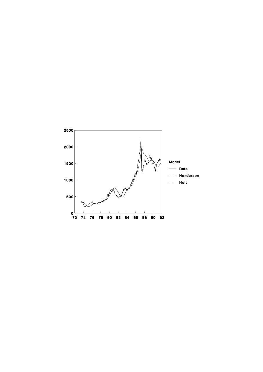
UNSW, July 2000 Draft, Decomposition of Time Series

moving average and Holt’s trend method with

α

= 0.1 and

β

= 0.1. It can be noted from

Figure 1.6 that Henderson’s method works well as a smoothing device over the range of

problems reflected in the share price data: changing trends, extreme values and changing

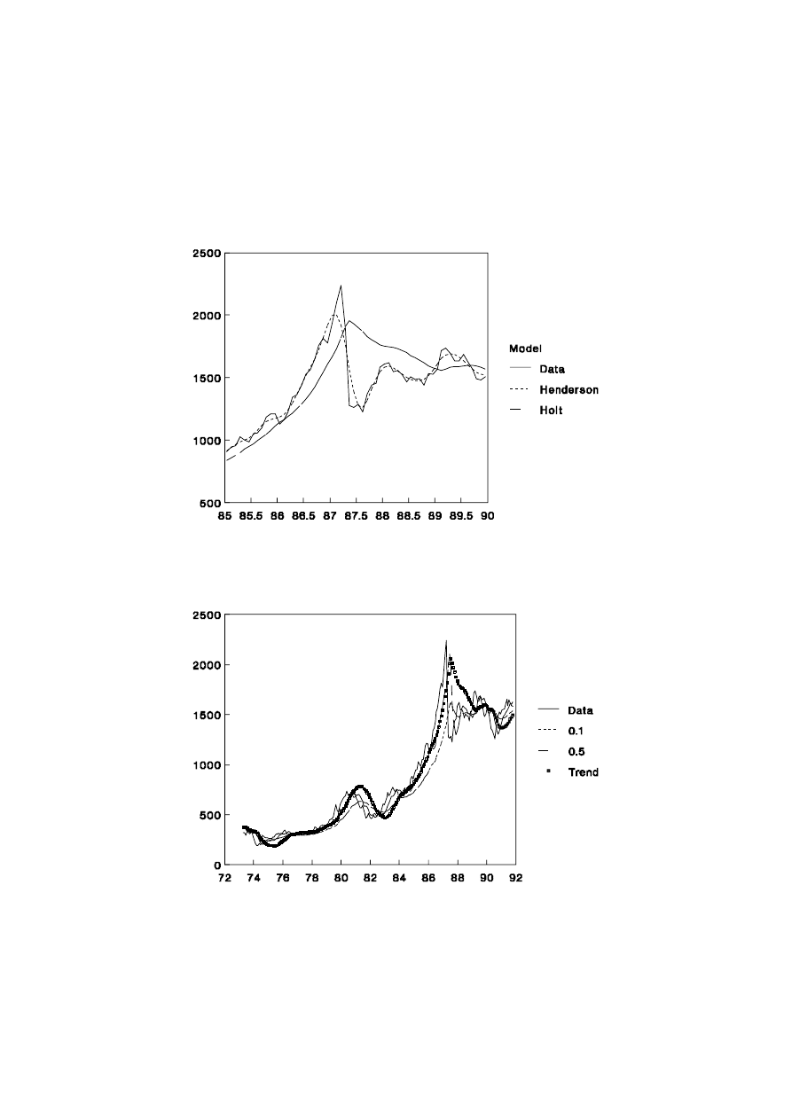
volatility. Holt’s method works much better than the EWMA with

α

= 0.1 during the

increasing trend of the 1980s shown in Figure 1.5 but it over-reacts after the share market

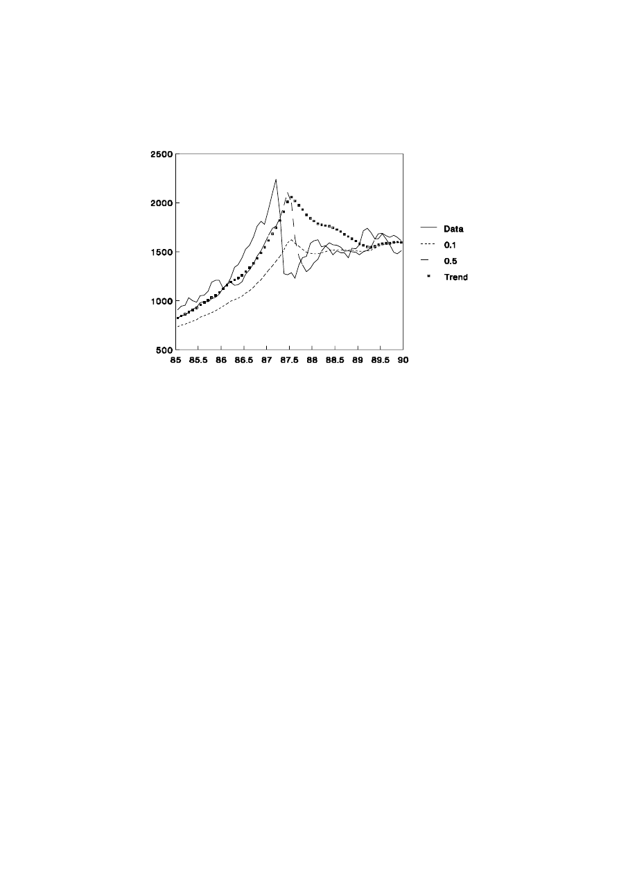
crisis of October 1987. These effects can be seen more clearly in Figure 1.7 which focuses

on the late 1980s.

Figure 1.6: Share Price Index and Trend Methods

In some sense, the comparison of the Henderson and Holt’s model, or indeed with

the EWMA models, should be qualified. Henderson’s method is not a forecasting tool but

the other methods have been presented as one-step forecasts. Thus, if Holt’s method is to

be used just as a smoothing model, the forecast yˆ

t

(1) should be replaced by m

t

. On the

other hand, if longer period forecasting is under consideration, even greater difference

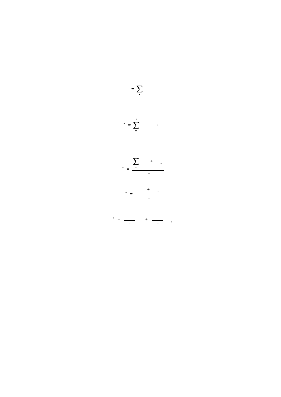
between the EWMA and Holt’s method can be noted. Three month ahead forecasts are

presented in Figures 1.8 and 1.9. Clearly, Holt’s model is inappropriate for share price

data and it is difficult to improve on an EWMA with a very large

α

, that is a model

which uses the current observation as the best forecast for all future time. If this were not

the case, investors would predict the future and alter the price of the shares accordingly.

22

Ronald Bewley, Time Series Forecasting

Such models are considered in greater detail in the more formal time series section of

these notes.

Figure 1.7: Performance of Trend Models During the 1980s

Figure 1.8: Three Month Forecasts of the Share Price Index

23

UNSW, July 2000 Draft, Decomposition of Time Series

Figure 1.9: Three Month Forecasts in the 1980s

24

Ronald Bewley, Time Series Forecasting

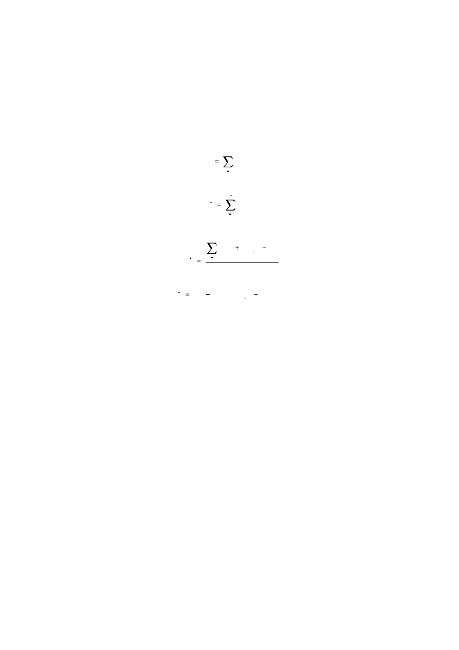
Appendix 1A: Updating of the Mean

If the mean of y

t

, m, is assumed constant, but its estimate, m

*

, is updated as new

data becomes available, the estimate with T observations

becomes

m

T

t 1

y

t

/T

with an additional observation. Moreover

m

T 1

t 1

y

t

/(T 1)

m

T

t 1

y

t

y

T 1

(T 1)

m

Tm

y

T 1

(T 1)

m













T

T 1

m













1

T 1

y

T 1

25

UNSW, July 2000 Draft, Decomposition of Time Series

Appendix 1B: Updating of Moving Averages

If the derivation from Appendix 1A is adapted for the T-period moving average

situation, that is one observation is dropped from the earliest period when the new data

point is added,

m

T

t 1

y

t

/T

m

T 1

t 2

y

t

/T

m

T

t 1

y

t

y

T 1

y

1

T

m

m

(1/T) y

T 1

(1/T) y

1

26

Ronald Bewley, Time Series Forecasting

Appendix 1C: Winter’s Method

If s is the period of seasonality (e.g. 12 with monthly data), Winter’s method can

be written as

m

T

=

α

(y

T

- F

T-s

) + (1-

α

) (m

T-1

+

τ

T-1

)

τ

T

=

β

(m

T

- m

T-1

) + (1-

β

)

τ

T-1

G

T

=

γ

(y

T

- m

T

) + (1-

γ

) G

T-s

F

T

(k) = (m

T

+ k

τ

T

) + G

T+k-s

for the additive model, where G

T

is the seasonal factor for observation T and

γ

is the

associated smoothing constant which is also between zero and one. G

T+k-s

is replaced by

G

T+k-2s

, etc if k > s.

The multiplicative model is

m

T

=

α

(y

T

/ F

T-s

) + (1-

α

) (m

T-1

+

τ

T-1

)

τ

T

=

β

(m

T

- m

T-1

) + (1-

β

)

τ

T-1

G

T

=

γ

(y

T

/ m

T

) + (1-

γ

) G

T-s

F

T

(k) = (m

T

+ k

τ

T

) G

T+k-s

27

UNSW, July 2000 Draft, Decomposition of Time Series

Appendix 1D: 13-term Henderson Weights

For all but the first and last six observations, the moving average is

m

t

= -0.014 y

t-6

- 0.028 y

t-5

+ 0.066 y

t-3

+ 0.147 y

t-2

+ 0.214 y

t-1

+ 0.240 y

t

+ 0.214 y

t+1

+ 0.147 y

t+2

+ 0.066 y

t+3

- 0.028 y

t+5

- 0.019 y

t+6

The last six terms are:

m

T-5

= -0.017 y

T-11

- 0.025 y

T-10

+ 0.001 y

T-9

+ 0.066 y

T-8

+ 0.147 y

T-7

+ 0.213 y

T-6

+ 0.238 y

T-5

+ 0.212 y

T-4

+ 0.144 y

T-3

+ 0.061 y

T-2

- 0.006 y

T-1

- 0.034 y

T

m

T-4

= -0.011 y

T-10

- 0.022 y

T-9

+ 0.003 y

T-8

+ 0.067 y

T-7

+ 0.145 y

T-6

+ 0.210 y

T-5

+ 0.235 y

T-4

+ 0.205 y

T-3

+ 0.136 y

T-2

+ 0.050 y

T-1

- 0.018 y

T

m

T-3

= -0.009 y

T-9

- 0.022 y

T-8

+ 0.004 y

T-7

+ 0.066 y

T-6

+ 0.145 y

T-5

+ 0.208 y

T-4

+ 0.230 y

T-3

+ 0.201 y

T-2

+ 0.131 y

T-1

+ 0.046 y

T

m

T-2

= -0.016 y

Y-8

- 0.025 y

T-7

+ 0.003 y

T-6

+ 0.068 y

T-5

+ 0.149 y

T-4

+ 0.216 y

T-3

+ 0.241 y

T-2

+ 0.216 y

T-1

+ 0.148 y

T

m

T-1

= -0.043 y

T-7

- 0.043 y

T-6

+ 0.002 y

T-5

+ 0.080 y

T-4

+ 0.174 y

T-3

+ 0.254 y

T-2

+ 0.292 y

T-1

+ 0.279 y

T

m

T

= -0.092 y

T-6

- 0.058 y

T-5

+ 0.012 y

T-4

+ 0.120 y

T-3

+ 0.244 y

T-2

+ 0.353 y

T-1

+ 0.421 y

T

28