Quick Start Tutorial
1-1
Quick Start Tutorial
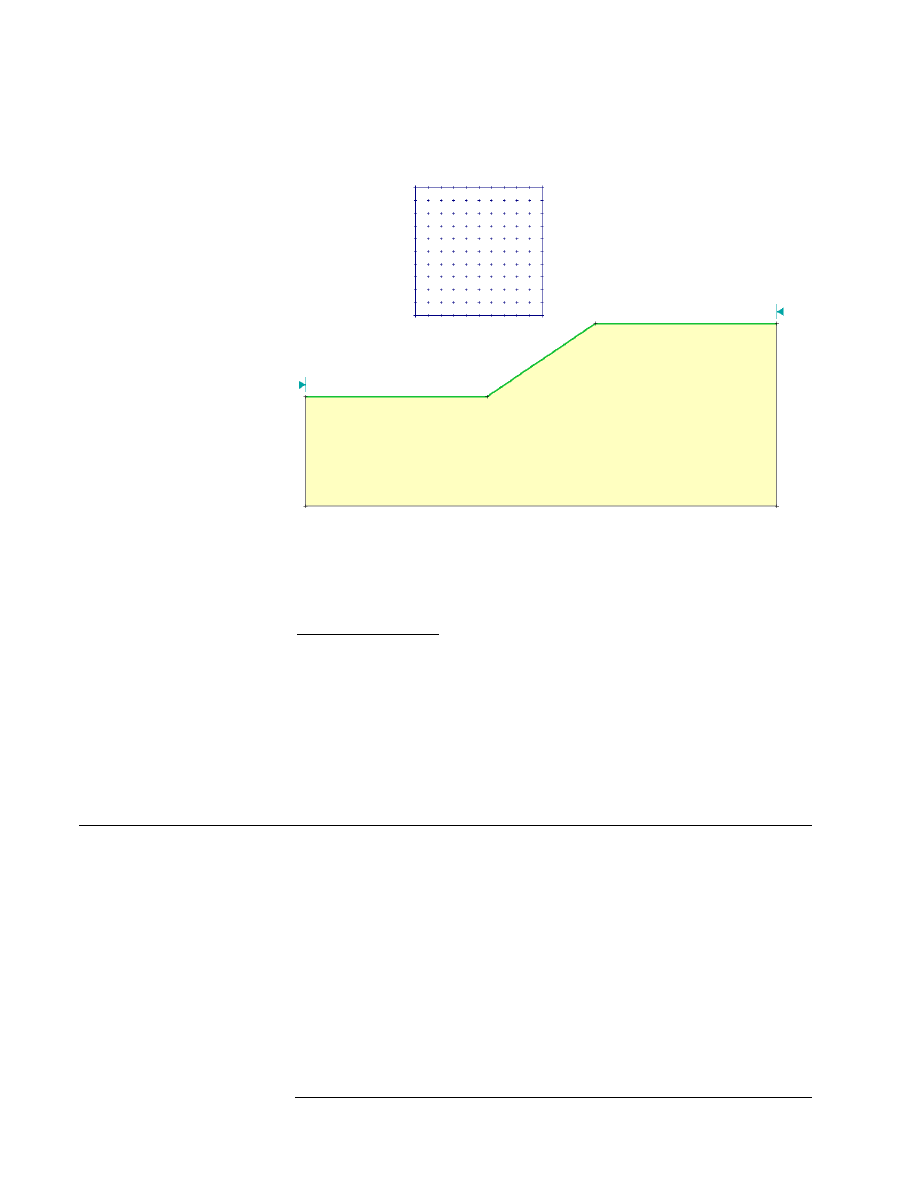
130 , 50
80 , 50
0 , 30
50 , 30
130 , 0
0 , 0
This “quick start” tutorial will demonstrate some of the basic features of
Slide using the simple model shown above. You will see how quickly and
easily a model can be created and analyzed with Slide.
MODEL FEATURES:
• homogeneous, single material slope
• no water pressure (dry)
• circular slip surface search (Grid Search)
The finished product of this tutorial can be found in the Tutorial 01
Quick Start.sli data file, located in the Examples > Tutorials folder in
your Slide installation folder.
Model
If you have not already done so, run the Slide Model program by double-
clicking on the Slide icon in your installation folder. Or from the Start
menu, select Programs
→ Rocscience → Slide 5.0 → Slide.
If the Slide application window is not already maximized, maximize it
now, so that the full screen is available for viewing the model.
Note that when the Slide Model program is started, a new blank
document is already opened, allowing you to begin creating a model
immediately.
Slide v.5.0 Tutorial
Manual
Quick Start Tutorial
1-2
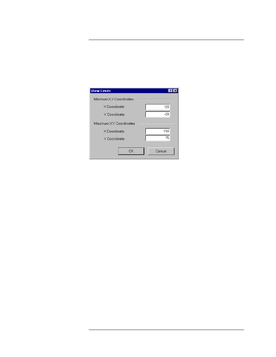
Limits
Let’s first set the limits of the drawing region, so that we can see the
model being created as we enter the geometry.
Select: View
→ Limits
Enter the following minimum and maximum x-y coordinates in the View
Limits dialog. Select OK.
Figure 1-1: View Limits dialog.
These limits will approximately center the model in the drawing region,
when you enter it as described below.
Slide v.5.0 Tutorial
Manual
Quick Start Tutorial
1-3
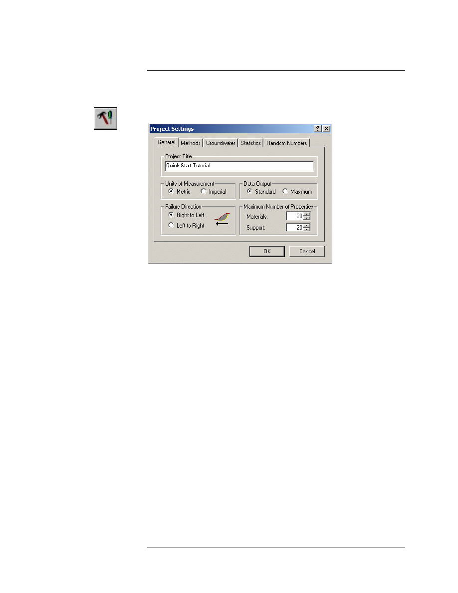
Project Settings
Although we do not need to set any Project Settings for this tutorial, let’s
briefly examine the Project Settings dialog.
Select: Analysis
→ Project Settings
Figure 1-2: Project Settings dialog.
Various important modeling and analysis options are set in the Project
Settings dialog, including Failure Direction, Units of Measurement,
Analysis Methods and Groundwater Method.
We will be using all of the default selections in Project Settings, however,
you may enter a Project Title – Quick Start Tutorial. Select OK.
Slide v.5.0 Tutorial
Manual
Quick Start Tutorial
1-4
Entering Boundaries
The first boundary that must be defined for every Slide model, is the
External Boundary.
The External Boundary in Slide is a closed polyline encompassing the
soil region you wish to analyze. In general:
An EXTERNAL BOUNDARY
must be defined for every
SLIDE model.
• The upper segments of the External Boundary represent the slope
surface you are analyzing.
• The left, right and lower extents of the External Boundary are
arbitrary, and can be extended as far out as the user deems necessary
for a complete analysis of the problem.
To add the External Boundary, select Add External Boundary from the
toolbar or the Boundaries menu.
Select: Boundaries
→ Add External Boundary
Enter the following coordinates in the prompt line at the bottom right of
the screen.
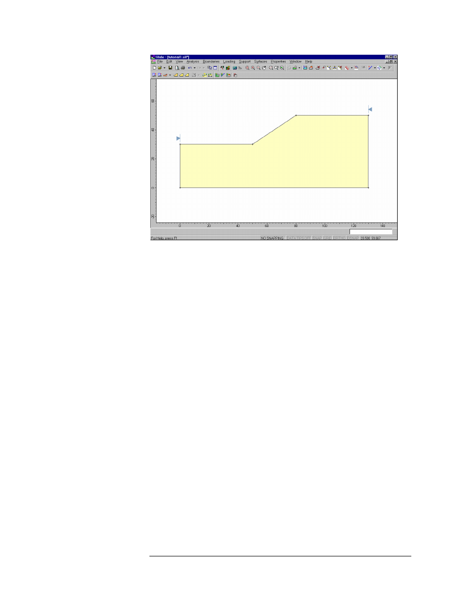
Enter vertex [esc=quit]: 0 0
Enter vertex [u=undo,esc=quit]: 130 0
Enter vertex [u=undo,esc=quit]: 130 50
Enter vertex [c=close,u=undo,esc=quit]: 80 50
Enter vertex [c=close,u=undo,esc=quit]: 50 30
Enter vertex [c=close,u=undo,esc=quit]: 0 30
Enter vertex [c=close,u=undo,esc=quit]: c
Note that entering c after the last vertex has been entered, automatically
connects the first and last vertices (closes the boundary), and exits the
Add External Boundary option.
Your screen should now look as follows:
Slide v.5.0 Tutorial
Manual
Quick Start Tutorial
1-5
Figure 1-3: External Boundary is created.
Note:
• Boundaries can also be entered graphically in Slide, by simply
clicking the left mouse button at the desired coordinates.
• The Snap options can be used for entering exact coordinates
graphically. See the Slide Help system for information about the
Snap options.
• Any combination of graphical and prompt line entry can be used to
enter boundary vertices.
Slide v.5.0 Tutorial
Manual
Quick Start Tutorial
1-6
Slip Surfaces
Slide can analyze the stability of either circular or non-circular slip
surfaces. Individual surfaces can be analyzed, or a critical surface search
can be performed, to attempt to find the slip surface with the lowest
factor of safety.
In this “quick start” tutorial, we will perform a critical surface search, for
circular slip surfaces. In Slide, there are 3 Search Methods available for
circular slip surfaces:
• Grid Search, Slope Search or Auto Refine Search.
We will use the Grid Search, which is the default method. A Grid Search
requires a grid of slip centers.
Auto Grid
Slip center grids can be user-defined (Add Grid option) or automatically
created by Slide (Auto Grid option). For this tutorial we will use the Auto
Grid option.
Select: Surfaces
→ Auto Grid
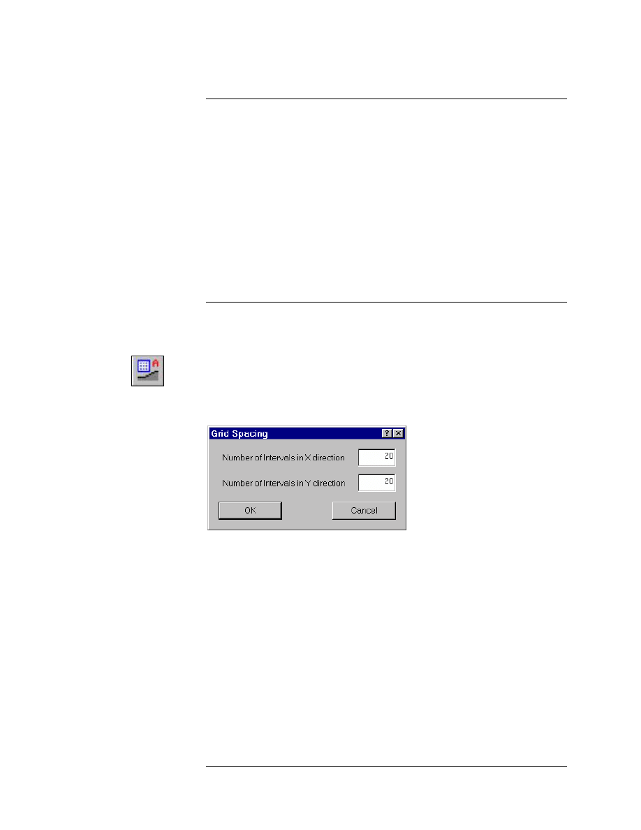
You will see the Grid Spacing dialog. We will use the default number of
intervals (20 x 20), so just select OK, and the grid will be created.
Figure 1-4: Grid Spacing dialog.
NOTE: By default, the actual locations of the slip centers within the grid
are not displayed. You can turn them on in the Display Options dialog.
Right-click the mouse and select Display Options from the popup menu.
Check the “Show grid points on search grid” option, and select Close.
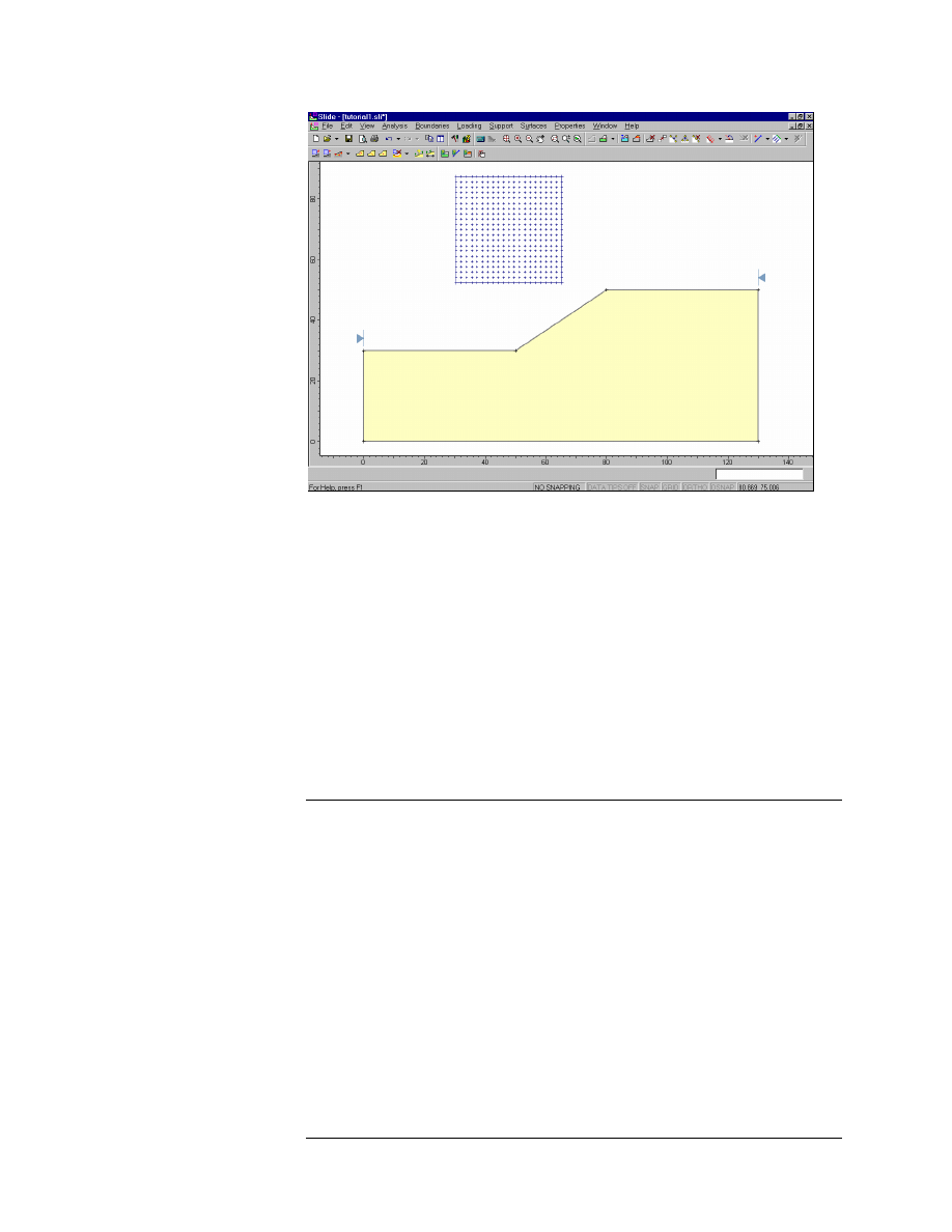
Your screen should look as follows.
Slide v.5.0 Tutorial
Manual
Quick Start Tutorial
1-7
Figure 1-5: Slip center grid created with Auto Grid.
Note that the 20 x 20 grid interval spacing actually gives a grid of 21 x 21
= 441 slip centers.
Each center in a slip center grid, represents the center of rotation of a
series of slip circles. Slide automatically determines the circle radii at
each grid point, based on the Slope Limits, and the Radius Increment.
The Radius Increment, entered in the Surface Options dialog, determines
the number of circles generated at each grid point.
How Slide performs a circular surface search, using the Slope Limits and
the Radius Increment, is discussed in the next section.
Slope Limits
When you created the External Boundary, you will notice the two
triangular markers displayed at the left and right limits of the upper
surface of the External Boundary. These are the Slope Limits.
The Slope Limits are automatically calculated by Slide as soon as the
External Boundary is created, or whenever editing operations (e.g.
moving vertices) are performed on the External Boundary.
The Slope Limits serve two purposes in a Slide circular surface analysis:
1. FILTERING – All slip surfaces must intersect the External
Boundary, within the Slope Limits. If the start and end points of a
slip surface are NOT within the Slope Limits, then the slip surface is
discarded (i.e. not analyzed). See Figure 1-6.
Slide v.5.0 Tutorial
Manual
Quick Start Tutorial
1-8
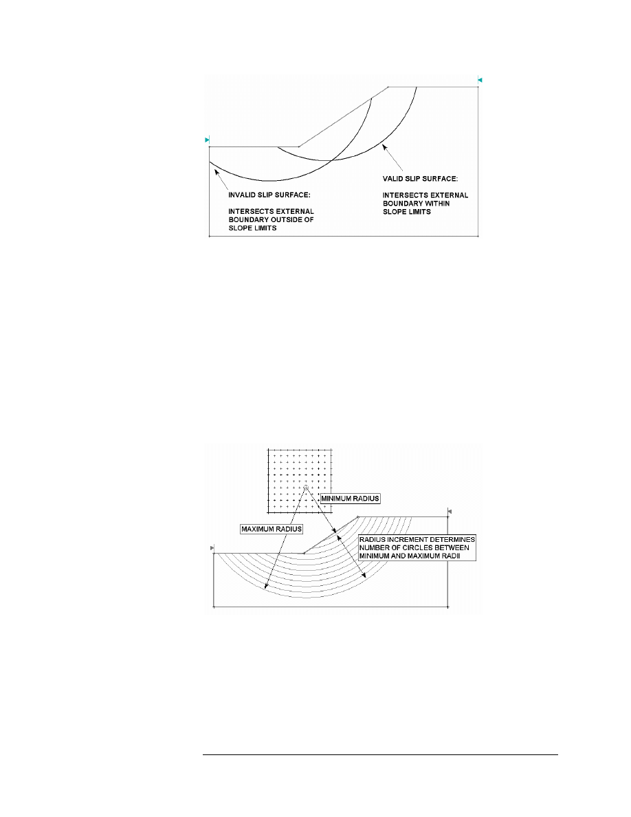
Figure 1-6: Slope Limits filtering for valid surfaces.
2. CIRCLE GENERATION – The sections of the External Boundary
between the Slope Limits define the slope surface to be analyzed. The
slope surface is used to generate the slip circles for a Grid Search, as
follows:
• For each slip center grid point, suitable Minimum and Maximum
radii are determined, based on the distances from the slip center
to the slope surface, as shown in Figure 1-7.
• The Radius Increment is then used to determine the number of
slip circles generated between the minimum and maximum radii
circles at each grid point.
Figure 1-7: Method of slip circle generation for Grid Search, using Slope Limits and
Radius Increment.
Slide v.5.0 Tutorial
Manual
Quick Start Tutorial
1-9
NOTE:
• The Radius Increment is the number of intervals between the
minimum and maximum circle radii at each grid point. Therefore the
number of slip circles generated at each grid point is equal to the
Radius Increment + 1.
• The total number of slip circles generated by a Grid Search, is
therefore = (Radius Increment + 1) x (total # of grid slip centers). For
this example, this equals 11 x 21 x 21 = 4851 slip circles.
Changing the Slope Limits
The default Slope Limits calculated by Slide will, in general, give the
maximum coverage for a Grid Search. If you wish to narrow the Grid
Search to more specific areas of the model, the Slope Limits can be
customized with the Define Limits dialog.
Select: Surfaces
→ Slope Limits → Define Limits
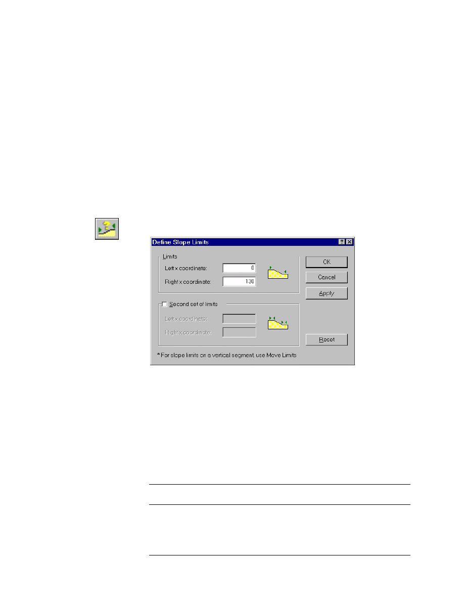
Figure 1-8: Define Slope Limits dialog.
The Define Slope Limits dialog allows the user to customize the left and
right Slope Limits, or even to define two sets of limits (e.g. to define
allowable ranges for slip surface starting and ending points).
We are using the default Slope Limits for this tutorial, however, it is
suggested that the user experiment with different Slope Limits, after
completing this tutorial.
Select Cancel in the Define Slope Limits dialog.
NOTE: the Slope Limits can also be moved graphically, using the mouse,
with the Move Limits option.
Slide v.5.0 Tutorial
Manual
Quick Start Tutorial
1-10
Surface Options
Let’s take a look at the Surface Options dialog.
Select: Surfaces
→ Surface Options
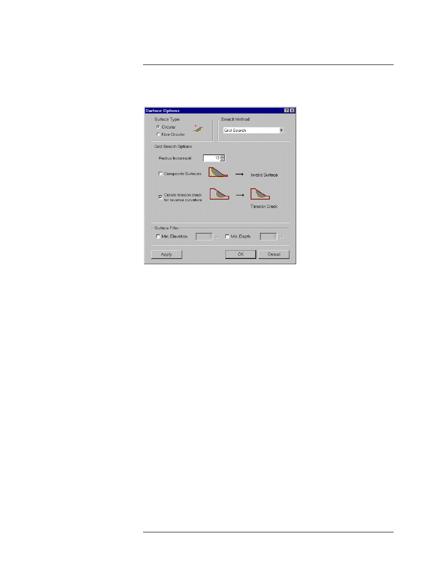
Figure 1-9: Surface Options dialog.
Note:
• The default Surface Type is Circular, which is what we are using for
this tutorial.
• The Radius Increment used for the Grid Search, is entered in this
dialog.
• The Composite Surfaces option is discussed in the Composite
Surfaces Tutorial.
We are using the default Surface Options, so select Cancel in the Surface
Options dialog.
Slide v.5.0 Tutorial
Manual
Quick Start Tutorial
1-11
Properties
Now let’s define the material properties.
Select: Properties
→ Define Materials
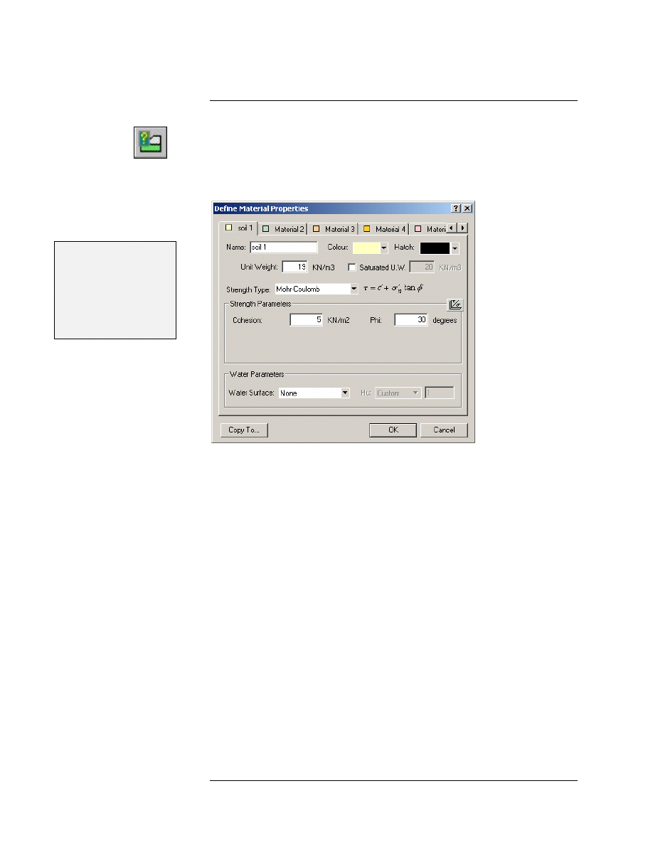
In the Define Material Properties dialog, enter the following parameters,
with the first (default) tab selected.
9 Enter:
9 Name = soil 1
9 Unit Weight = 19
Strength Type = Mohr-Coul
9 Cohesion = 5
9 Phi = 30
Water Surface = None
Figure 1-10: Define Material Properties dialog.
When you are finished entering properties, select OK.
NOTE: Since we are dealing with a single material model, and since you
entered properties with the first (default) tab selected, you do not have to
Assign these properties to the model. Slide automatically assigns the
default properties (i.e. the properties of the first material in the Define
Material Properties dialog) for you.
(Remember that when you created the External Boundary, the area
inside the boundary was automatically filled with the colour of the first
material in the Define Material Properties dialog. This represents the
default property assignment.)
For multiple material models, it is necessary for the user to assign
properties with the Assign Properties option. We will deal with assigning
properties in Tutorial 2.
Slide v.5.0 Tutorial
Manual
Quick Start Tutorial
1-12
Analysis Methods
Before we run the analysis, let’s examine the Analysis Methods that are
available in Slide.
Select: Analysis
→ Project Settings
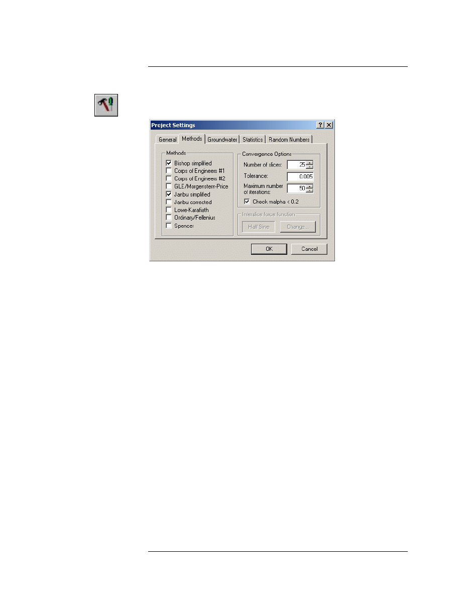
Figure 1-11: Analysis Methods dialog.
Select the Methods tab in the Project Settings dialog.
By default, Bishop and Janbu limit equilibrium analysis methods, are the
selected Analysis Methods.
However, the user may select any or all analysis methods, and all
selected methods will be run when Compute is selected. See the Slide
Help system for information about the different analysis methods, and
the assumptions used in each.
For this tutorial, we will only use the default analysis methods – Bishop
and Janbu. Select Cancel in the Project Settings dialog.
We are now finished with the modeling, and can proceed to run the
analysis and interpret the results.
Slide v.5.0 Tutorial
Manual
Quick Start Tutorial
1-13
Compute
Before you analyze your model, save it as a file called quick.sli. (Slide
model files have a .SLI filename extension).
Select: File
→ Save
Use the Save As dialog to save the file. You are now ready to run the
analysis.
Select: Analysis
→ Compute
The Slide COMPUTE engine will proceed in running the analysis. This
should only take a few seconds. When completed, you are ready to view
the results in INTERPRET.
Slide v.5.0 Tutorial
Manual
Quick Start Tutorial
1-14
Interpret
To view the results of the analysis:
Select: Analysis
→ Interpret
This will start the Slide INTERPRET program. You should see the
following figure:
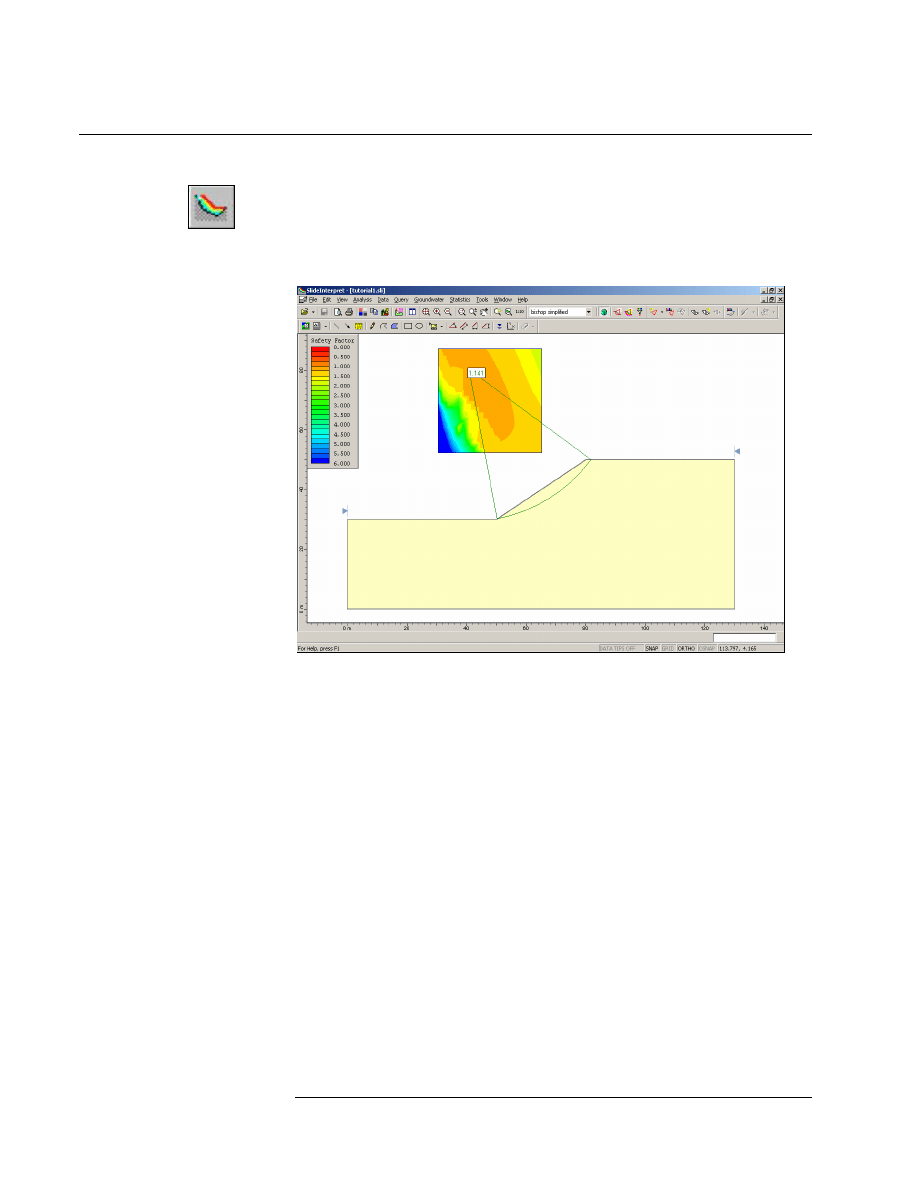
Figure 1-12: Results of Grid Search.
By default, when a computed file is first opened in the Slide
INTERPRETER, you will always see:
• The Global Minimum slip surface, for the BISHOP Simplified
analysis method (if a Bishop analysis was run)
• If a Grid Search has been performed, you will see contours of safety
factor in the slip center grid. The contours are based on the
MINIMUM calculated safety factor at each grid slip center.
The Global Minimum slip surface, and the contoured grid are both visible
in Figure 1-12.
Slide v.5.0 Tutorial
Manual
Quick Start Tutorial
1-15
Global Minimum Slip Surfaces
For a given analysis method, the Global Minimum slip surface is the slip
surface with the LOWEST factor of safety, of all slip surfaces analyzed.
The analysis method is displayed in the Toolbar at the top of the Slide
INTERPRET screen.
The Global Minimum safety factor is displayed beside the slip center for
the surface. In this case, for a Bishop analysis, the overall minimum
safety factor is 1.141.
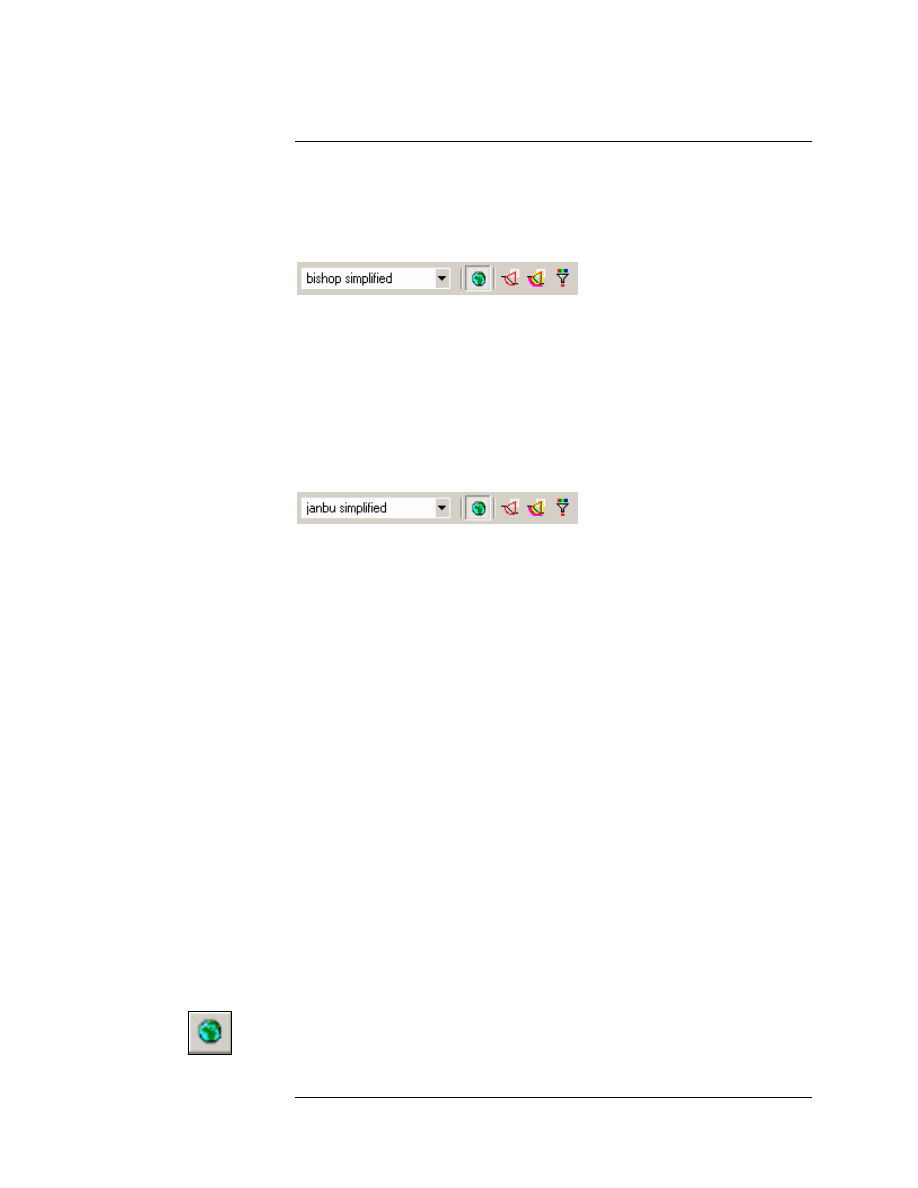
To view the Global Minimum safety factor and surface for other analysis
methods, simply use the mouse to select a method from the drop-down
list in the toolbar. For example, select the Janbu Simplified method, and
observe the results. In general, the Global Minimum safety factor and
slip surface, can be different for each analysis method.
Tip – while the analysis method is selected in the toolbar, if you have a
mouse with a mouse wheel, you can scroll through the analysis methods
by moving the mouse wheel. This allows you to quickly compare analysis
results, without having to select the analysis method each time.
It is very important to note the following –
• The term “Global Minimum” should be used with caution. The Global
Minimum surfaces displayed after an analysis, are only as good as
your search techniques, and may not necessarily be the lowest
possible safety factor surfaces for a given model. Depending on your
search methods and parameters, SURFACES WITH LOWER
SAFETY FACTORS MAY EXIST!!! (For example, grid location, grid
interval spacing, Radius Increment and Slope Limits, will all affect
the results of the Grid Search.)
Also note –
• In the current example, for the Bishop and Janbu analysis methods,
the Global Minimum surface is the same for both methods.
HOWEVER, IN GENERAL, THE GLOBAL MINIMUM SURFACE
FOR EACH ANALYSIS METHOD, WILL NOT NECESSARILY BE
THE SAME SURFACE!!!
The display of the Global Minimum surface, may be toggled on or off by
selecting the Global Minimum option from the toolbar or the Data menu.
Select: Data
→ Global Minimum
Slide v.5.0 Tutorial
Manual
Quick Start Tutorial
1-16
The Global Minimum is hidden.
Select: Data
→ Global Minimum
The Global Minimum is displayed.
Viewing Minimum Surfaces
Remember that the Grid Search is performed by generating circles of
different radii at each grid point in a slip center grid.
To view the minimum safety factor surface generated AT EACH GRID
POINT, select the Minimum Surfaces option in the toolbar or the Data
menu.
Select: Data
→ Minimum Surfaces
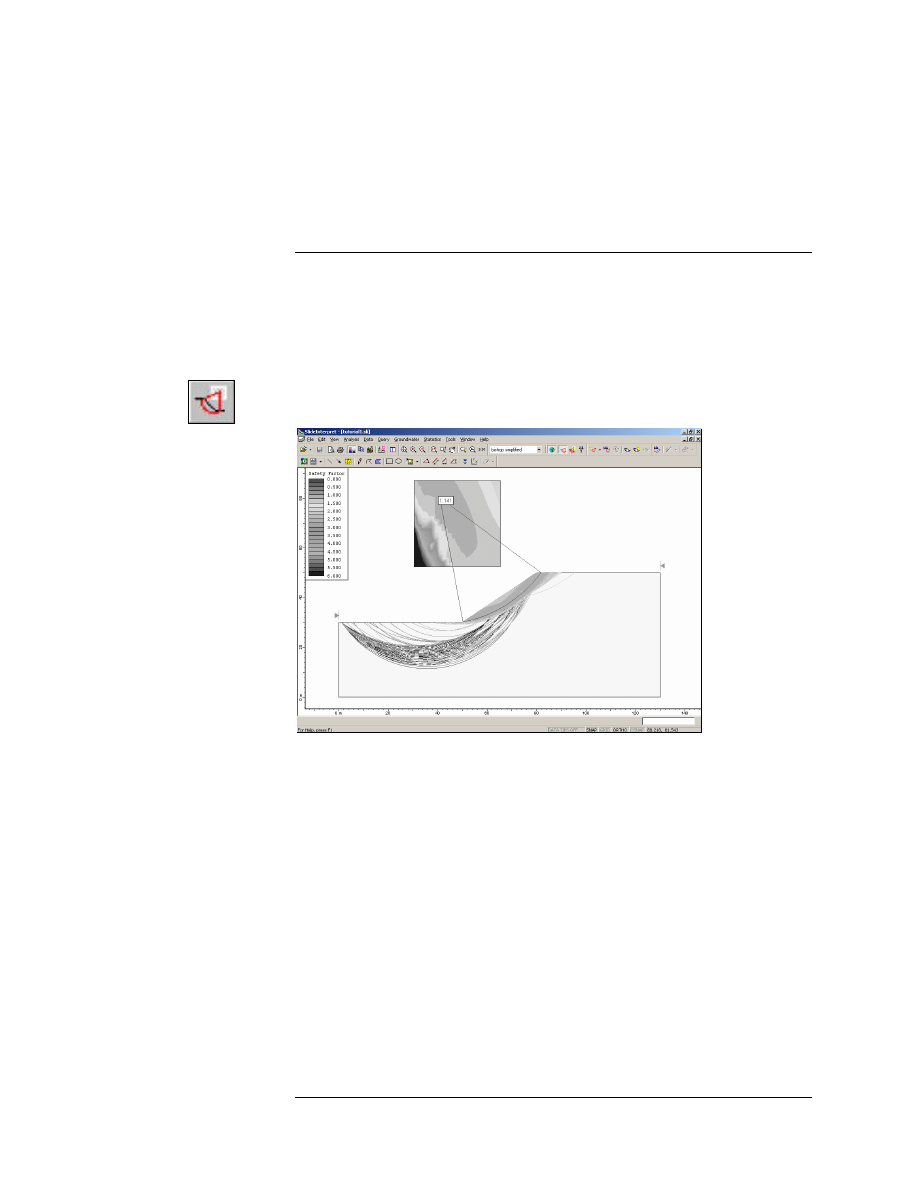
Figure 1-13: Circular surface search – Mimimum Surfaces shown.
As shown in Figure 1-13, Slide will draw the minimum slip surfaces, with
colours corresponding to the safety factor contours in the grid, and in the
legend (visible in the upper left corner).
Again, as with the Global Minimum, note that the Minimum Surfaces
correspond to the currently selected analysis method. (i.e. if you select
different analysis methods, you may see different surfaces displayed).
Slide v.5.0 Tutorial
Manual
Quick Start Tutorial
1-17
Viewing All Surfaces
To view ALL valid slip surfaces generated by the analysis, select the All
Surfaces option from the toolbar or the Data menu.
Select: Data
→ All Surfaces
Again, note that the slip surfaces are colour coded according to safety
factor, and that safety factors will vary according to the analysis method
chosen.
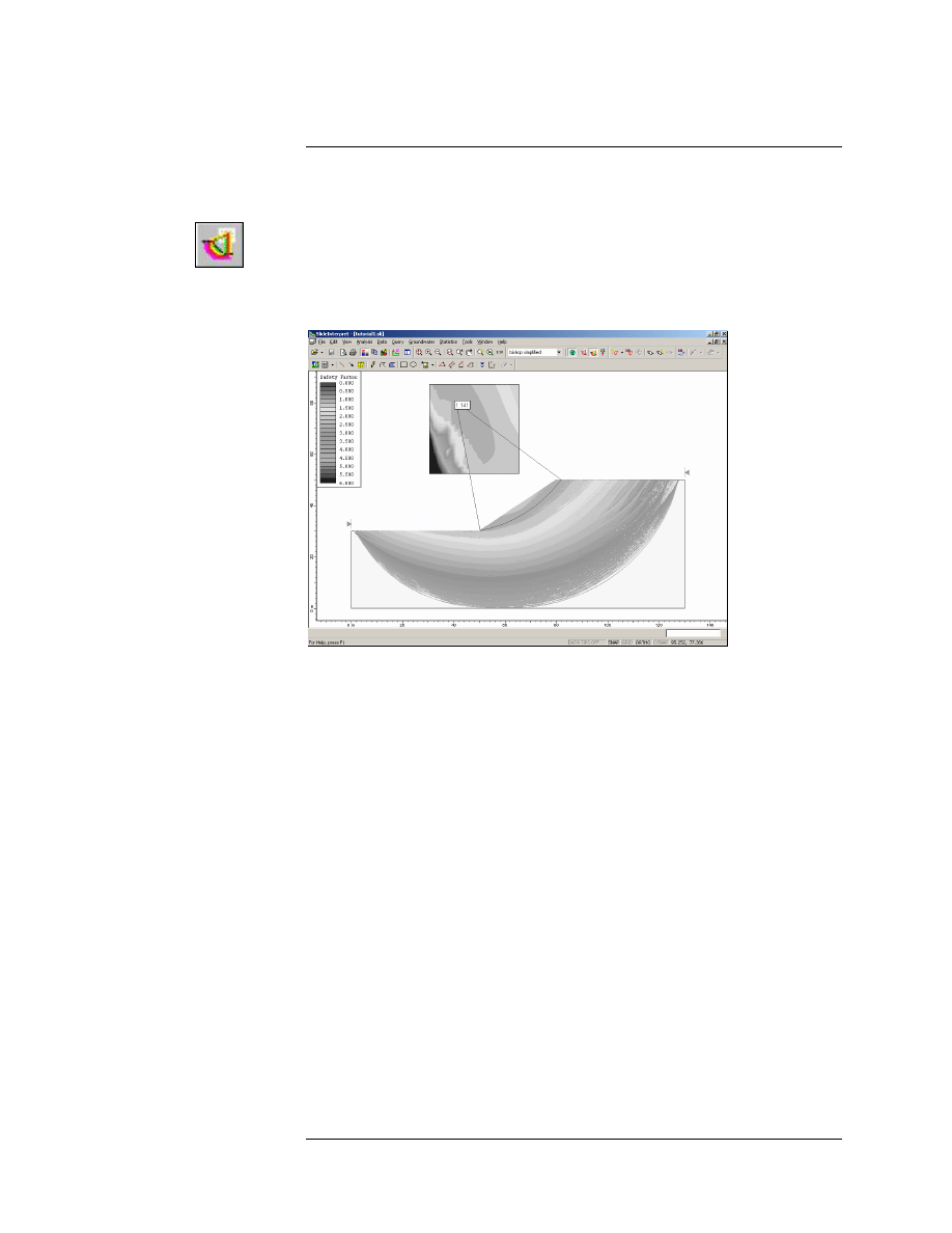
Figure 1-14: Circular surface search – All Surfaces shown.
NOTE: since the slip surfaces overlap, Slide draws the slip surfaces
starting with the HIGHEST safety factors, and ending with the LOWEST
safety factors, so that the slip surfaces with the lowest safety factors are
always visible (i.e. they are drawn last).
The All Surfaces option is very useful for visualizing all of the valid
surfaces generated by your analysis. It may indicate:
• areas in which to concentrate a search, in order to find a lower Global
Minimum, using some of the various techniques provided in Slide.
For example, customizing the Slope Limits, as discussed earlier in
this tutorial, or using the Focus Search options in the Surfaces menu.
• areas which have been insufficiently covered by the search, again,
necessitating a change in the search parameters (e.g. location of the
slip center grid, or a larger value of Radius Increment).
Slide v.5.0 Tutorial
Manual
Quick Start Tutorial
1-18
Filter Surfaces
When displaying either the Minimum Surfaces, or All Surfaces, as
described above, you can filter the surfaces you would like displayed,
using the Filter Surfaces option in the toolbar or the Data menu.
Select: Data
→ Filter Surfaces
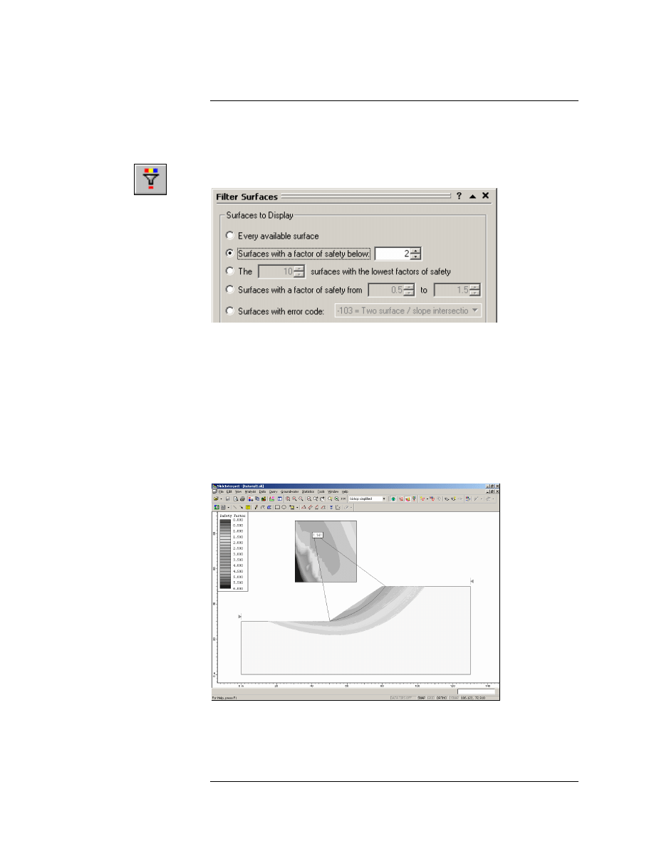
Figure 1-15: Filter Surfaces option.
Filtering can be done by safety factor, or by a specified number of lowest
surfaces (e.g. the 10 lowest safety factor surfaces). To see the results of
applying the filter parameters, without closing the dialog, use the Apply
button.
For example, select the “Surfaces with a factor of safety below” option.
Leave the default safety factor value of 2. Only surfaces with a factor of
safety less than 2 are now displayed. Select Done.
Figure 1-16: All slip surfaces with safety factor < 2.
Slide v.5.0 Tutorial
Manual
Quick Start Tutorial
1-19
Data Tips
The Data Tips feature in Slide allows the user to obtain model and
analysis information by simply placing the mouse cursor over any model
entity or location on the screen.
To enable Data Tips, click on the box on the Status Bar (at the bottom of
the Slide application window), which says Data Tips. By default, it
should indicate Data Tips Off. When you click on this box, it will toggle
through 3 different data tip modes – Off, Min and Max. Click on this box
until it displays Data Tips Max.
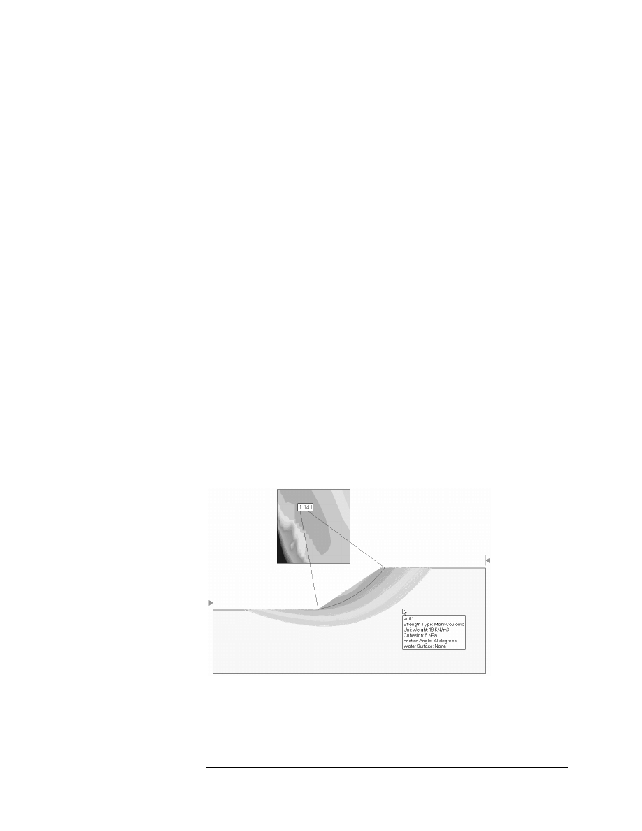
Now move the mouse cursor over the model, and you will see that the
material properties of the soil are displayed. Place the cursor over
different entities of the model, and see what information is displayed.
Virtually all model information is available using Data Tips, for example:
• slip surface safety factor, center and radius
• vertex coordinates
• grid coordinates
• contour values within slip center grids
• slope limit coordinates
• support properties
• etc etc
Click on the Status Bar and toggle Data Tips Off. You can experiment
with the Data Tips option in later tutorials. NOTE that Data Tips can
also be toggled through the View menu.
Figure 1-17: Data Tips display of material properties.
Slide v.5.0 Tutorial
Manual
Quick Start Tutorial
1-20
Info Viewer
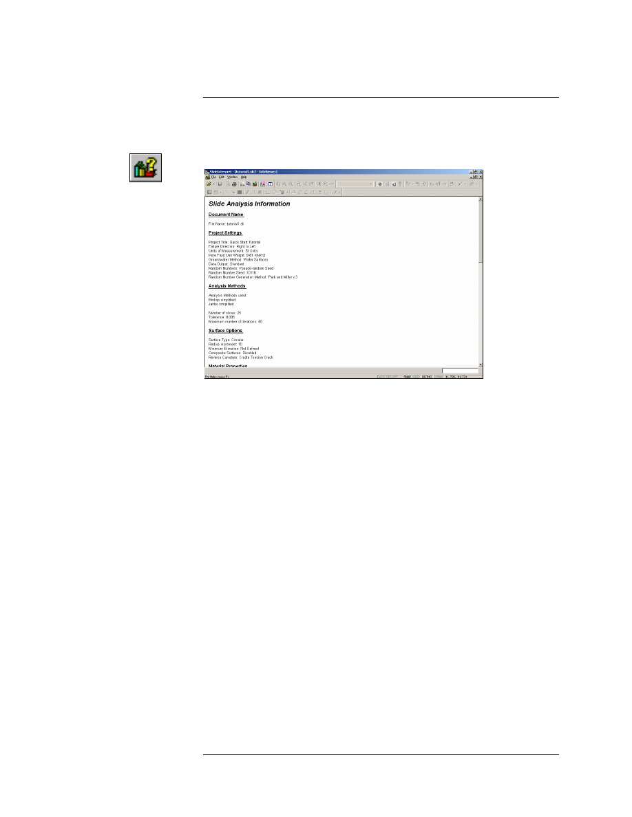
The Info Viewer option in the toolbar or the Analysis menu, displays a
summary of Slide model and analysis information, in its own view.
Select: Analysis
→ Info Viewer
Figure 1-18: SLIDE Info Viewer listing.
The Info Viewer information can be copied to the clipboard using the
Copy option in the toolbar or the Edit menu, or by right-clicking in the
view and selecting Copy. From the clipboard, the information can be
pasted into word processing programs for report writing.
The Info Viewer information can also be saved to a text file (*.txt – plain
text, no formatting preserved), or a rich-text file (*.rtf – preserves
formatting, as displayed in the Info Viewer). The Save As text file options
are available in the File menu, (while the Info Viewer is the active view),
or by right-clicking in the Info Viewer view.
The Info Viewer information can also be sent directly to your printer
using the Print option in the toolbar or File menu.
Close the Info Viewer view, by selecting the X in the upper right corner of
the view.
Slide v.5.0 Tutorial
Manual
Quick Start Tutorial
1-21
Drawing Tools
In the Tools menu or the toolbar, a wide variety of drawing and
annotation options are available for customizing views. We will briefly
demonstrate some of these options.
First, let’s add an arrow to the view, pointing at the Global Minimum
surface. Select the Arrow option from the Tools toolbar or the Tools
menu.
Select: Tools
→ Add Tool → Arrow
Click the mouse at two points on the screen, to add an arrow pointing at
the Global Minimum surface. Now add some text.
Select: Tools
→ Add Tool → Text Box
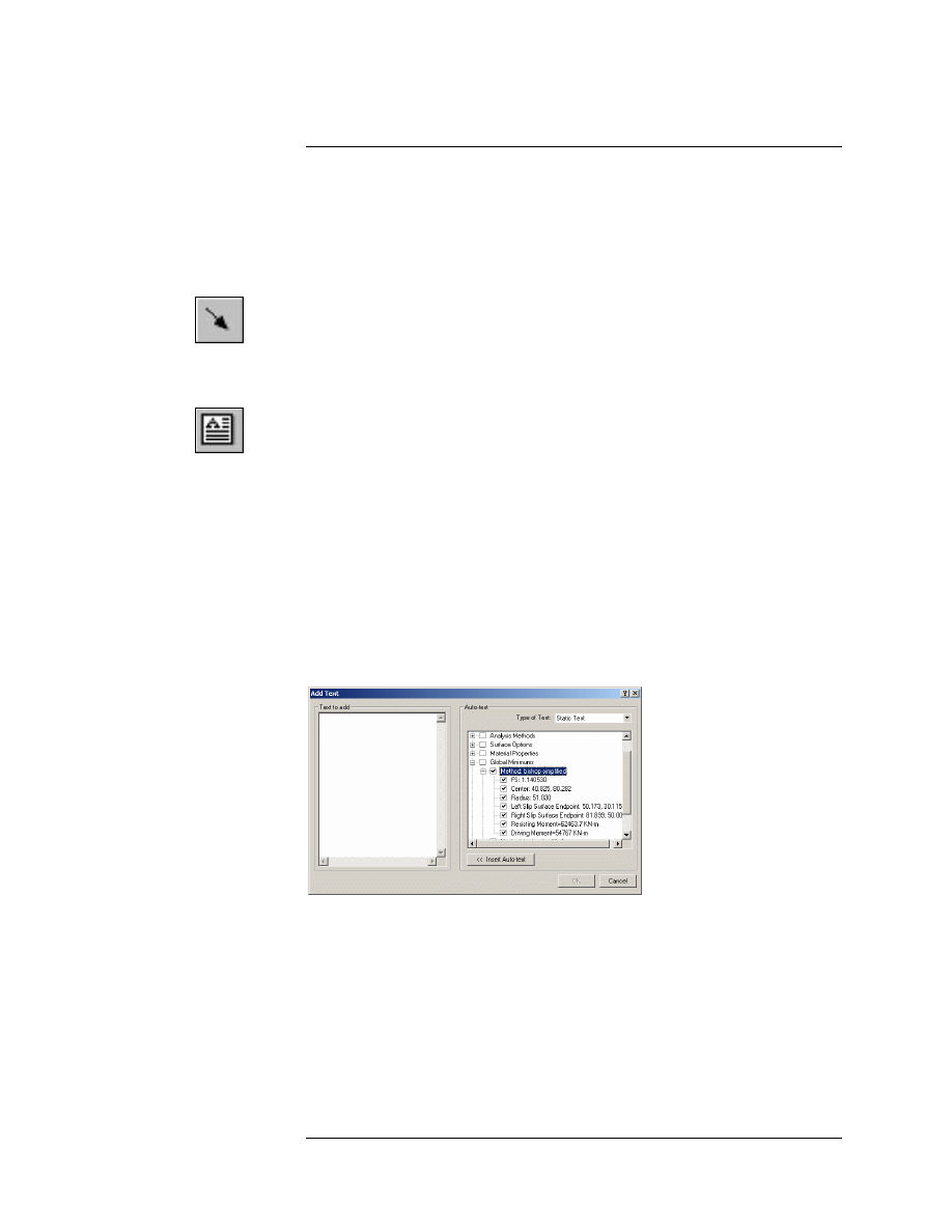
Click the mouse at a point near the tail of the arrow. You will see the Add
Text dialog. The Add Text dialog allows you to type any text and add it to
the screen. The convenient Auto-Text option can be used to annotate the
model with pre-formatted input and output data.
For example:
1. In the Add Text dialog, select the Global Minimum “+” box (NOT the
checkbox). Then select the Method: Bishop Simplified “+” box. Then
select the Method: Bishop Simplified checkbox.
2. The dialog should appear as follows:
Figure 1-19: Add Text dialog.
3. Now select the Insert Auto-text button. The Global Minimum surface
information for the Bishop analysis method, will be added to the
editing area at the left of the Add Text dialog.
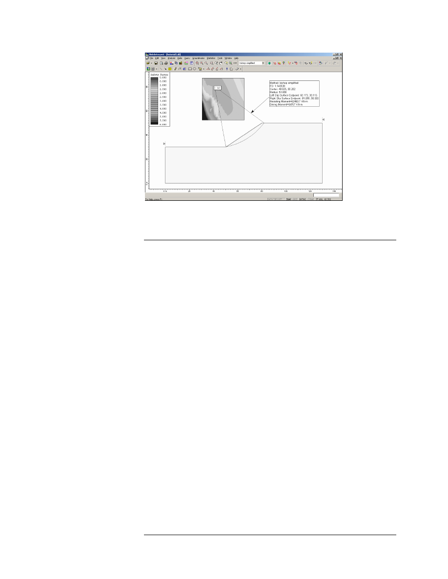
4. Now select OK. The text is added to the view, and your screen should
look similar to Figure 1-20.
Slide v.5.0 Tutorial
Manual
Quick Start Tutorial
1-22
Figure 1-20: Auto-text and arrow added to view.
Editing Drawing Tools
We will now describe the following properties of all drawing tools added
through the Tools menu options:
Right-click
If you right-click the mouse on a drawing tool, you will see a popup menu,
which makes available various editing options.
For example:
• right-click on the arrow. Delete, Format and Duplicate options are
available in the popup menu.
• right-click on the text box. Various options are available, including
Format, Edit Text, Rotate and Delete.
Single-click
If you single-click the left mouse button on a drawing tool, this will
“select” the tool, and you will see the “control points” highlighted on the
tool. While in this mode:
• You can click and drag the control points, to re-size the tool.
• If you hover the mouse over any part of the drawing tool, but NOT on
a control point, you will see the four-way arrow cursor, allowing you
to click and drag the entire drawing tool to a new location.
• You can delete the tool by pressing Delete on the keyboard.
Slide v.5.0 Tutorial
Manual

Quick Start Tutorial
1-23
Double-click
If you double-click the mouse on a drawing tool, you will see the Format
Tool dialog. The Format Tool dialog allows the user to customize styles,
colours etc. Only the options applicable to the clicked-on tool, will be
enabled in the Format Tool dialog. (Note: this is the same Format option
available when you right-click on a tool).
It is left as an optional exercise, for the user to experiment with the
various editing options that are available for each Tools option.
Saving Drawing Tools
All drawing tools added to a view through the Tools menu, can be saved,
so that you do not have to re-create drawings each time you open a file.
• The Save Tools option in the toolbar or the File menu, will
automatically save a tools file with the same name as the
corresponding Slide file. In this case, the tools file will automatically
be opened when the Slide file is opened in INTERPRET, and you will
immediately see the saved drawing tools on the opening view.
• The Export Tools option in the File menu, can be used to save a tools
file with a DIFFERENT name from the original Slide file. In this
case, you will have to use the Import Tools option to display the tools
on the model. This allows you, for example, to save different tools
files, corresponding to various views of a model.
• Tools files have a *.SLT filename extension
NOTE: when you save a TOOLS file, only drawing tools of the current
(active) view are saved.
Slide v.5.0 Tutorial
Manual
Quick Start Tutorial
1-24
Slide v.5.0 Tutorial
Manual
Exporting Images
In Slide, various options are available for exporting image files.
Export Image
The Export Image option in the File menu or the right-click menu, allows
the user to save the current view directly to one of four image file
formats:
• JPEG (*.jpg)
• Windows Bitmap (*.bmp)
• Windows Enhanced Metafile (*.emf)
• Windows Metafile (*.wmf)
Copy to Clipboard
The current view can also be copied to the Windows clipboard using the
Copy option in the toolbar or the Edit menu. This will place a bitmap
image on the clipboard which can be pasted directly into word or image
processing applications.
Black and White Images (Grayscale)
The Grayscale option, available in the toolbar or the View menu, will
automatically convert the current view to Grayscale, suitable for black
and white image requirements. This is useful when sending images to a
black and white printer, or for capturing black and white image files.
The Grayscale option works as a toggle, and all previous colour settings
of the current view will be restored when Grayscale is toggled off
We have now covered most of the basic features in the Slide INTERPRET
program, except the ability to obtain detailed analysis information for
individual slip surfaces, using the Query menu options. This is covered in
the next tutorial.
That concludes this Quick Start Tutorial. To exit the program:
Select: File
→ Exit
Document Outline
Wyszukiwarka
Podobne podstrony:
01 ENVI Quick Start
HUAWEI B593u 12 Quick Start(V100R001 01)
Pro drive Quick Start
,Voice Quick Start
Blender ENG Tutorial 01 Cartoonish Landscape
01 Linux Start systemu i związanie z nim procesy
borland c++builder 6 quick start 5GXKEOAPPJEUZ3BARU7TLRFBSSUSGQDKNS33OKA
Hackmaster Quick Start Rules
ANSYS quick start
CoC Dark Ages Quick Start
Parallels Desktop Mac Quick Start Guide
Quick Start Guide
2 SATA150 TX2 TX4 quick start v1 2
Smart Box NVR Series Quick Start Guide V1 0 0
E583X S quick start
Quick Start Guide
16 0 ANSYS Quick Start Licensing Guide
więcej podobnych podstron