Anshumana And Kalay Can Splits Create Market Liquidity Theory And Evidence

Journal of Financial Markets 5 (2002) 83–125

Can splits create market liquidity?

Theory and evidence

V. Ravi Anshuman

*, Avner Kalay

b,c

Finance and Control, Indian Institute of Management, Bannerghatta Road, Bangalore 560 076, India

The Leon Recanati Graduate School of Business Administration, Tel Aviv University,

P.O.B. 39010, Ramat Aviv, Tel Aviv 69978, Israel

Department of Finance, David Eccles School of Business, University of Utah, Salt Lake City,

UT 84112, USA

Abstract

We present a market microstructure model of stock splits in the presence of minimum

tick size rules. The key feature of the model is that discretionary trading is endogenously
determined. There exists a tradeoﬀ between adverse selection costs on the one hand and
discreteness related costs and opportunity costs of monitoring the market on the other
hand. Under certain parameter values, there exists an optimal price. We document an
inverse relation between the coeﬃcient of variation of intraday trading volume and the
stock price level. This empirical evidence and other existing evidence are consistent with
the model. r 2002 Elsevier Science B.V. All rights reserved.

JEL classiﬁcation:

G12; G18; G32

Keywords:

Stock splits; Liquidity; Tick size; Discreteness; Trading range; Optimal price

This paper draws on the Ph.D. dissertation of V. Ravi Anshuman and an earlier joint working

paper. We have received helpful comments from Larry Glosten, Ishwar Murty, Avanidhar
Subrahmanyam (the editor) and anonymous referees. We would also like to thank J. Coles, T.
Callahan, S. Ethier, R. Lease, U. Loewenstein, S. Manaster, J. Suay, E. Tashjian, S. Titman, Z.
Zhang, and seminar participants at Ben Gurion University, Boston College, Carnegie Mellon
University, Cornell University, Hebrew University, Hong Kong University of Science and
Technology, Rutgers University, Tel Aviv University, University of Utah and the European
Finance Association meetings for their helpful comments. The ﬁrst author acknowledges support
from the Global Business Program, University of Utah and the Recanati Graduate School of
Business, Tel Aviv University, Hong Kong University of Science and Technology, and the
University of Texas at Austin. We take responsibility for any remaining errors.

*Corresponding author. Tel.: +91-80-699-3104; fax: +91-80-658-4050.

E-mail address:

anshuman@iimb.ernet.in (V.R. Anshuman).

1386-4181/02/$ - see front matter r 2002 Elsevier Science B.V. All rights reserved.
PII: S 1 3 8 6 - 4 1 8 1 ( 0 1 ) 0 0 0 2 0 - 9

1. Introduction

U.S. ﬁrms split their stocks quite frequently. In spite of inﬂation, positive

real interest rates, and signiﬁcant risk premiums, the average nominal stock
price in the U.S. during the past 50 years has been almost constant. Why would
ﬁrms keep on splitting their stocks to maintain low prices?This behavior is
puzzling since, by doing so, ﬁrms actively increase their eﬀective tick size (i.e.,
tick size/price), potentially exposing their stockholders to larger transaction
costs.

This paper presents a value maximizing market microstructure model of

stock splits. Our model joins practitioners in predicting that ﬁrms split their
stocks to move the stock price into an optimal trading range in order to
improve liquidity.

1,2

The driving force of the model stems from the fact that

prices on U.S. exchanges are restricted to multiples of 1/8th of a dollar.

This

restriction on prices creates a wedge between the ‘‘true’’ equilibrium price and
the observed price.

Thus a portion of the transaction costs incurred by traders

is purely an artifact of discreteness.

Anshuman and Kalay (1998) show that discreteness related commissions

depend on the location of the ‘‘true’’ equilibrium price on the real line. In other
words, whether the discrete pricing restriction is binding or not depends on the
location of the ‘‘true’’ equilibrium price relative to a legitimate price (tick) in a
discrete price economy. It may so happen that the ‘‘true’’ equilibrium price
(plus any transaction cost) is close to a tick. Discreteness related commissions
would be low in such a period. As information arrives in the market, the
location of the ‘‘true’’ equilibrium price changes, and discreteness related
commissions would, therefore, vary over time. They could be as low as 0 or as
high as the tick size.

Interestingly, liquidity traders can take advantage of the variation in

discreteness related commissions by timing their trades. Of course, such

Academicians have mostly relied on signaling models to explain stock splits (Grinblatt et al.,

1984). More recently, Muscarella and Vetsuypens (1996) provide evidence consistent with the
liquidity motive of stock splits. Practitioners, however, have all along held the belief that stock
splits help restore an optimal trading range that maximizes the liquidity of the stock (see Baker and
Powell, 1992; Bacon and Shin, 1993).

Independent of our work, Angel (1997) has also presented a model of optimal price level that

explains stock splits. In his model, the optimal price provides a tradeoﬀ between ﬁrm visibility and
transaction costs. In contrast, our model examines the behavior of liquidity traders in the presence
of discrete pricing restrictions.

There are exceptions to this restriction and more recently the NYSE has initiated a move

toward decimal trading.

The ‘‘true’’ equilibrium price is the market value of the asset conditional on all publicly

available information in an otherwise identical continuous-price economy without any frictions
(transaction costs).

V.R. Anshuman, A. Kalay / Journal of Financial Markets 5 (2002) 83–125

strategic behavior is not costless. It involves close monitoring of the market
to take advantage of periods with low discreteness related commissions.
In general, liquidity traders diﬀer in terms of their opportunity costs of
monitoring the market. Some liquidity traders may prefer not to time the
market because the beneﬁts from timing trades do not oﬀset their opportunity
costs of monitoring. In contrast, other liquidity traders who are endowed with
low opportunity costs of monitoring may ﬁnd it beneﬁcial to time their trades.
Such discretionary traders would trade together in a period of low discreteness
related commissions. The presence of additional liquidity traders in this period
(a period of concentrated trading) forces the competitive market maker to
charge a lower adverse selection commission than otherwise. Thus, discre-
tionary liquidity traders save on execution costs – adverse selection as well as
discreteness related commissions.

Because the tick size is ﬁxed in nominal terms (at 1/8th of a dollar), the

economic signiﬁcance of the savings in discreteness related commissions
depends on the stock price level. At low stock price levels, the savings in
execution costs due to timing of trades may be signiﬁcant enough to oﬀset the
opportunity costs of monitoring of most liquidity traders. There would be
highly concentrated trading at low price levels as most liquidity traders would
exercise the ﬂexibility of timing trades. Conversely, at high stock price levels,
few liquidity traders would time trades because the potential savings in
execution costs are economically insigniﬁcant.

The key implication of the model is that the stock price level aﬀects the

distribution of liquidity trades across time, and consequently, the transaction
costs incurred by them. In particular, we show that there exists an optimal
stock price level that induces an optimal amount of discretionary trading. This
optimal price results in the lowest (total) expected transaction costs incurred by
all liquidity traders.

Because investors desire liquidity (Amihud and Mendelson, 1986; Brennan

and Subrahmanyam, 1995), a value-maximizing ﬁrm should choose a stock
price level that maximizes liquidity (minimizes the total transaction costs
incurred by all liquidity traders). By splitting (or reverse splitting) its stock, a
ﬁrm can always reset its stock price to the optimal price level.

We present numerical solutions of the model to show that, under certain

parameter values, an optimal price exists. The numerical solutions show that
the optimal price is increasing in the volatility of the underlying asset and
decreasing in the fraction of liquidity traders. We also show that the
optimal price is (linearly) increasing in the tick size. Finally, using intraday
transaction data, we document a cross-sectional inverse relation between the
coeﬃcient of variation of time-aggregated trading volume (a measure of the
degree of concentrated trading in a stock) and the stock price level.
This empirical evidence and other existing evidence are consistent with the
model.

V.R. Anshuman, A. Kalay / Journal of Financial Markets 5 (2002) 83–125

The paper is organized as follows. Section 2 discusses a numerical example

that illustrates the key features of the model. The model is developed in
Section 3. Section 4 presents numerical solutions of the model. Section 5
discusses empirical evidence relevant to the model, and Section 6 concludes the
paper.

2. A numerical example

Consider the following example that illustrates the central theme of the

model – endogenization of discretionary trading. We make the following
simplifying assumptions in the numerical example. (i) There are two trading
opportunities (Periods 1 and 2). (ii) Discreteness related commissions in each
period are either $0.02 or $0.10 with equal probability.

(iii) Firms are

restricted to choose between two base prices ($50 or $100) – the base price
could be thought of as the oﬀer price in an initial public oﬀering. (iv) Liquidity
traders are of two types: 80 liquidity traders face very low opportunity costs of
monitoring ($0.01 per dollar of trade) and 40 liquidity traders face extremely
high opportunity costs of monitoring. (v) In each period, there are a ﬁxed
number of informed traders who speculate on information that is revealed at
the end of the period.

Before the market opens, liquidity traders face a strategic choice. They know

that monitoring the market can help them time their trades into the period with
low discreteness related commissions ($0.02). Not only would they be saving on
discreteness related commissions but also on adverse selection commissions
because of the concentration of liquidity trades in a single period.

However, monitoring the market is not costless. Among the liquidity traders,

those with extremely high monitoring costs would not ﬁnd timing trades
worthwhile. Such liquidity traders (40) behave like nondiscretionary traders.
Assuming that there are negligible waiting costs, these traders would be
indiﬀerent between trading in Period 1 or trading in Period 2. Let equal
number of nondiscretionary traders (40/2=20) arrive in the market in each
period.

The interesting question is with regard to the 80 liquidity traders with low

monitoring costs. Should they incur monitoring costs and time their trades or
join the bandwagon of nondiscretionary traders?If they choose not to monitor
(and, therefore, act as nondiscretionary traders), then each trading period
would consist of (80+40)/2=60 liquidity traders, assuming that the arrival
rate of nondiscretionary traders is constant (equal) in both periods. On the
other hand, if these liquidity traders choose to monitor, one of the trading

This assumption is purely for illustration purposes. In reality, there exists a probability

distribution of discreteness related commissions over the interval (0, tick size).

V.R. Anshuman, A. Kalay / Journal of Financial Markets 5 (2002) 83–125

periods would have 100 (80 discretionary and 20 nondiscretionary) liquidity
traders, and the other period would have only 20 nondiscretionary liquidity
traders. Hence the distribution of liquidity traders across the two periods
would be one of the following: (60, 60) if they choose not to monitor the market
and either (20, 100) or (100, 20) if they monitor the market.

Liquidity traders with low monitoring costs would think as follows. Their

choice to monitor or not depends on the total (per dollar) transaction costs
they face under each scenario. Total transaction costs are composed of adverse
selection commissions, discreteness related commissions, and monitoring costs.
Table 1 presents these costs at the two base prices in this economy.

Consider Panel A of Table 1 for the case when the base price is $50. Suppose

liquidity traders with low monitoring costs choose to monitor the market. Then,
in the period they trade, the adverse selection commissions would be low
because of the presence of 100 liquidity traders. In contrast, when they choose
not to monitor the market, the adverse selection commissions are going to be
higher because there would be only 60 liquidity traders. Assume that the adverse
selection commissions are $0.046 when there are 100 liquidity traders and
$0.535 when there are 60 liquidity traders (in the model, we derive the adverse
selection commissions endogenously). Monitoring the market and concentrat-
ing trades in a single period results in savings of ($0.535 $0.046)=$0.489 in
adverse selection commissions, or 0.978% of the base price of $50.

Panel B of Table 1 shows the adverse selection commissions when the base

price is $100. These numbers are scaled up versions of the adverse selection
commissions when the base price is $50. However, as shown in the (%) adverse
selection commission column, the adverse selection commissions (given a ﬁxed
number of liquidity trades) are identical at both base prices in percentage
terms. Therefore, the beneﬁt of concentrated trading (in terms of savings in
adverse selection commissions) is 0.978%, which is invariant to the base price.

Now consider discreteness related commissions when the base price is $50

(Panel A). If liquidity traders with low monitoring costs choose to monitor,
they would incur lower discreteness related commissions because they can time
their trades in the period with low discreteness related commissions ($0.02).
Note that they would incur expected discreteness related commissions of $0.04
(this is higher than $0.02 because it is always possible that both trading periods
have a realized discreteness related commission of $0.10).

In contrast, when

such liquidity traders choose not to monitor, they incur a higher expected
discreteness related commission of $0.06 (an average of $0.02 and $0.10). These
commissions ($ values) stay the same at the higher base price of $100 (Panel B).

The probability of both trading periods having high discreteness related commissions ($0.10) is

0.5 0.5=0.25. The probability of at least one period having low discreteness related commissions
($0.02) is 10.25=0.75. Therefore, the expected discreteness related commissions is 0.25
$0.10+0.75 $0.02=$0.04.

V.R. Anshuman, A. Kalay / Journal of Financial Markets 5 (2002) 83–125

Because discreteness causes ﬁxed costs, the beneﬁt of timing trades (due to

savings in discreteness related commissions) is ﬁxed at $0.06$0.04=$0.02
independent of the base price. However, on a per dollar basis, the savings from
timing trades are 0.04% at the lower base price of $50, but only 0.02% at the
higher base price of $100.

Table 1
Numerical example

Liquidity traders are of two types – those who incur low monitoring costs (80) and those who incur

high monitoring costs (40). This numerical example illustrates the decision-making of liquidity
traders with low monitoring costs. If these liquidity traders choose to monitor the market, the
number of liquidity traders across the two periods would either be (100, 20) or (20, 100). If they
choose not to monitor, the number of liquidity traders in each period would be 60. At a base price
of $50, it is better to monitor because the total transaction costs are lower (Panel A). Conversely, at
a base price of $100, it is better not to monitor (Panel B). The total transaction costs incurred by all
liquidity traders (nondiscretionary and discretionary) is shown in Panel C.

Panel A: Decision to monitor the market

(base price is $50)

Adverse
selection
commissions

Discreteness
related
commissions

Monitoring
costs
(per dollar)

Total
transaction
costs
(per dollar)

Monitor

Liquidity
traders

($)

(%)

($)

(%)

Yes

100

0.046

0.092

0.04

0.080

1.000

1.172

0.535

1.070

0.06

0.120

0.000

1.190

Savings

0.489

0.978

0.02

0.040

1.000

0.018

Panel B: Decision to monitor the market

(base price is $100)

Adverse selection
commissions

Discreteness
related
commissions

Monitoring
costs

Total
transaction
costs

Monitor

Liquidity
traders

($)

(%)

($)

(%)

Yes

100

0.092

0.04

0.040

1.000

1.132

1.07

1.070

0.06

0.060

0.000

1.130

Savings

0.978

0.02

0.020

1.000

0.002

Panel C: Total transaction costs incurred by ALL liquidity traders

Base
price

Distribution of trades

Adverse
selection
costs

Discreteness
related costs

Monitoring
costs

Total
transaction
costs

$50

(100, 20) or (20, 100)

0.322

0.112

0.800

1.234

$100

(60, 60)

1.284

0.072

0.000

1.356

V.R. Anshuman, A. Kalay / Journal of Financial Markets 5 (2002) 83–125

Besides adverse selection commissions and discreteness related commissions,

liquidity traders also incur monitoring costs (1%) if they choose to monitor.
When the base price is $50 (Panel A), the sum of adverse selection
commissions, discreteness related commissions and monitoring costs is
1.172% upon monitoring and 1.19% without monitoring. When the base
price is $100 (Panel B), the total transaction costs are 1.132% upon monitoring
and 1.130% without monitoring.

The decision to monitor or not depends on the total savings in transaction

costs shown in the bottom row of Panels A and B in Table 1. At a lower base
price of $50, monitoring is preferred because the total savings are 0.018%. In
contrast, at a higher base price of $100, it is better not to monitor because the
savings are 0.002%.

The key to the model is the diﬀerence in the nature of the two components of

(dollar) execution costs – (dollar) adverse selection and (dollar) discreteness
related commissions. The former increases in proportion to the base price
whereas the latter, being ﬁxed, stays the same at all price levels. Therefore,
discretionary liquidity are indiﬀerent about the price level with respect to the
savings in adverse selection commissions (0.978% at both base prices).
However, they do care about the price level with respect to savings in
discreteness related commissions (0.02% at the higher base price of $100, but
0.04% at the lower base price of $50).

At the lower base price of $50, the savings in discreteness related

commissions are suﬃciently high, and total savings in execution costs (adverse
selection and discreteness related commissions) oﬀset monitoring costs.
Monitoring the market is therefore beneﬁcial to liquidity traders with low
monitoring costs. In contrast, at the higher base price of $100, monitoring is
not

beneﬁcial. Hence, liquidity traders with low monitoring costs endogenously

choose to act as discretionary traders when the base price is $50, but prefer to
act as nondiscretionary traders when the base price is $100. As a result, when
the base price is $50, the trading pattern across the two periods is either (100,
20) or (20, 100). In contrast, when the base price is $100, the trading pattern is
(60, 60). Thus, the base price level aﬀects the distribution of liquidity traders
across the two periods.

Panel C in Table 1 shows the total transaction costs due to adverse selection,

discreteness, and monitoring incurred by all liquidity traders at the two base
prices. For the computations in Panel C of Table 1, we assume that the adverse
selection commission is $0.575 when the number of liquidity traders in a
period is 20. This situation arises in one of the periods when the base
price is $50. To read Panel C in Table 1, consider the ﬁrst row where the base
price is $50. 100 liquidity traders face an adverse selection commission of
$0.046 and 20 liquidity traders face an adverse selection commission of $0.575.
On a per dollar basis, the total adverse selection commissions are
[100 $0.046+ 20 $0.575]/$50=0.322. We refer to this sum of all adverse

V.R. Anshuman, A. Kalay / Journal of Financial Markets 5 (2002) 83–125

selection commissions as the adverse selection component of total transaction
costs.

Furthermore, 100 liquidity traders face discreteness related commissions of

$0.04 and 20 liquidity traders face discreteness related commissions of $0.08
(this is less than $0.10 because they may be just lucky and trade in a period with
discreteness related commissions of $0.02). The total discreteness related
commissions on a per dollar basis is [100 $0.04+20 $0.08]/$50=0.112 (we
refer to the sum of all discreteness related commissions as the discreteness
related component of total transaction costs).

Finally, 80 liquidity traders incur monitoring costs of 1%, implying

total monitoring costs of [80 (0.01 $50)/$50]=0.80 on a per dollar basis.
This is the monitoring cost component of total transaction costs. The total
transaction costs are [0.322+0.112+0.80]=1.234 on a per dollar basis. Note
that this is the total transaction cost of all liquidity traders, taken together as a
group.

In contrast, when the base price is $100, the total transaction costs (on a per

dollar basis) are 1.356. From the ﬁrm’s perspective, the lower base price of $50
is preferable because liquidity traders (nondiscretionary and discretionary,
taken together as a group) face lower total transaction costs on a per dollar
basis.

Panel C in Table 1 also shows that the adverse selection component is

increasing in the base price. This situation arises because a lower base price is
associated with more concentrated trading. Consequently, many liquidity
traders incur low adverse selection commissions, resulting in a lower adverse
selection component. In contrast, the discreteness related and the monitoring
cost components are decreasing in the base price. This opposite relationship
provides the tradeoﬀs for an optimal price level.

In contrast to the numerical example, the model allows for a continuum of

monitoring costs for liquidity traders, a continuum of discreteness related
commissions, a continuum of base prices, and multiple (although, ﬁnite)
rounds of trading opportunities. More importantly, the adverse selection and
discreteness related commissions are endogenously determined.

The intuition of the model can also be explained as follows. A lower

base price induces more liquidity traders to act as discretionary traders.
This is beneﬁcial because greater discretionary trading results in a
lower adverse selection component. However, a lower base price also has
adverse cost implications. First, the discreteness related commission (DRC)
component increases and higher (cumulative) monitoring costs are incurred
because more liquidity traders act as discretionary traders. The optimal price,
which results in an optimal amount of discretionary trading, is the one
equating the marginal adverse selection component on the one hand to the sum
of the marginal DRC and the marginal monitoring cost component on the
other hand.

V.R. Anshuman, A. Kalay / Journal of Financial Markets 5 (2002) 83–125

3. The model

This section develops a market microstructure model that captures the role

of the asset price level in determining the behavior of market participants. The
asset price process is given by P

¼ P

t
t¼

; where P

is the underlying

asset price at time t; P

is an initial base price and d

½ Nð0; s

Þ represents an

unanticipated piece of (short-lived) private information that is revealed at the
end of each period t:

We also assume that s is linear in the base price, i.e., sðP

Þ ¼ kP

; where k is

referred to as the volatility parameter.

This characterization recognizes that

the magnitude of private information released in each period is proportional to
the underlying asset value. The rest of the economy is characterized by the
following assumptions:

(A1) The size of the trading population is T and there are m trading periods.
(A2) Risk neutral market makers post competitive prices before accepting

order ﬂow. Market makers do not incur order processing costs and do not face
any inventory constraints.

(A3) A fraction (1 l) of the trading population (T ) consists of cash

constrained risk neutral informed traders who trade on short-lived information
in each one of the m periods. They obtain (identical) perfect signals of d

at the

beginning of each period t:

(A4) A fraction l of the trading population (T) consists of risk neutral

uninformed liquidity traders.

A2 ensures that market makers post ask and bid prices such that the

expected losses to informed traders are oﬀset by the expected proﬁts from
uninformed liquidity traders (as in Admati and Pﬂeiderer, 1989). A3 implies
that informed traders cannot assume unbounded positions to take advantage
of the perfect signal because of wealth constraints (again, as in Admati and
Pﬂeiderer, 1989). Their order size is normalized to 1 for convenience. Note, d is
short-lived information that is revealed at the end of each period. Therefore, in
order to utilize their (exogenously) acquired private information, informed
traders must trade in the same period they receive information. For
convenience, we assume that in each period, tAð1; mÞ; the same informed
traders are observing a private signal (d

) and taking positions based upon this

information.

Our assumption of linearity is consistent with the standard assumption in asset pricing

literature. It mathematically follows that splitting an asset into n equal parts results in the standard
deviation of each part being equal to (1/n)th the standard deviation of the original asset. In other
words, standard deviation is linearly related to underlying asset value.

V.R. Anshuman, A. Kalay / Journal of Financial Markets 5 (2002) 83–125

3.1. Equilibrium commissions

Consider the ask side of the market (the analysis is identical for the bid side

of the market). For the competitive, risk neutral market maker, the equilibrium
ask commission (a

) can be determined by setting his expected proﬁts to zero.

Given A3, the number of informed traders in each period is ð1 lÞT: For
purposes of illustration let the remaining uninformed liquidity traders (lT ) be
equally distributed across the m periods. Then, we get the equilibrium
commission (a

) by solving the following equation (see Appendix A for the

derivation):

ð1 lÞT sðP

Þf

1 F

a ¼

ð1Þ

where fð:Þ and Fð:Þ represent the probability density function and the
cumulative distribution function of the standard normal distribution,
respectively. The left hand side of Eq. (1) shows the expected proﬁts of the
market makers, which is made up of two components – the ﬁrst term represents
the expected losses to informed traders and the second term represents the
expected proﬁts from liquidity traders.

Note that T factors out of Eq. (1). Thus, the trading population (T ) is

irrelevant for the analysis. Also, if a

is the solution to Eq. (1), then, under

continuous prices, the ask price (A

) is equal to P

þ a

: We refer to a

as the

adverse selection commission. Because sðP

Þ increases linearly in P

; it turns

out that the (dollar) adverse selection commission (a

) also increases linearly in

: However, as shown in Appendix A the adverse selection commission per

dollar traded

(i.e., percentage commissions) is constant and independent of the

base price (P

3.2. Discreteness related commissions (DRC)

Under discrete prices (separated by ticks of size d), the market maker’s

pricing policy is diﬀerent. In all likelihood, it may not be feasible to set the
price at A

¼ P

þ a

because A

may not be an exact multiple of the tick

size (d). Anshuman and Kalay (1998) show that, under discrete prices,
competitive market makers round the ask price upward to the nearest feasible
price (similarly, on the bid side of the market, the continuous-case bid price is
rounded downward to the nearest feasible price).

Therefore, the discreteness

Anshuman and Kalay (1998) examine the impact of discrete pricing restrictions in greater detail.

Following them, we assume that there can be no cross-subsidization of proﬁts across time, i.e.,
market makers could sell below a

in one period and sell above a

in the other period, thereby,

selling at an average commission of a

: Such a linear combination of trades, i.e., splitting orders

and executing them at adjacent prices, is assumed to be very costly. Alternatively, one can assume
that the market maker is not allowed to use mixed strategies in his pricing rule.

V.R. Anshuman, A. Kalay / Journal of Financial Markets 5 (2002) 83–125

related commissions on the ask side of the market are equal to d2Mod½P

; d (if Mod½P

þ a

; d > 0) or equal to 0 (if Mod½P

þ a

; d ¼ 0).

The restriction on discreteness of prices results in a few interesting

implications. First, due to discreteness, there is an additional component of
transaction costs, henceforth referred to as DRC. The equilibrium commission
is going to vary in the range [a

; a

þ d), depending on the location of A

ð¼ P

þ a

Þ on the real line. Second, given that P

and a

are common

knowledge at time t; all market participants can infer the exact magnitude of
DRC

in the current period.

3.3. Strategic liquidity trading

Liquidity traders can reduce transaction costs by deferring their trades to a

period where DRC are very low. More importantly, they would also face lower
adverse selection commissions because of the ensuing concentration of trades.
The beneﬁts of strategically timing trades can be a signiﬁcant reduction in
execution costs.

Of course, such strategic behavior is not costless. It involves close

monitoring of the market to take advantage of periods with low DRC. The
monitoring costs for a liquidity trader depends on the opportunity cost of his
or her time. From here on, we recognize that liquidity traders face diﬀerential
opportunity costs of monitoring.

(A5) At time t ¼ p; risk neutral liquidity traders (lT) make a strategic

decision – whether to act as discretionary or nondiscretionary traders. This
decison depends on their personal opportunity costs of monitoring. We assume
that, on a continuum of increasing monitoring costs, the qth percentile liquidity
trader incurs a (per dollar) monitoring cost, CðqÞ ¼ f =½lnðqÞ

1=w

; where f > 0

and w > 1:

At time t ¼ p; all liquidity traders are potential discretionary traders.

Liquidity traders weigh the beneﬁts of discretionary trading (namely, lower
execution costs) against their personal opportunity costs of monitoring. Only
those liquidity traders who foresee a net beneﬁt choose to act as discretionary
traders. We assume that, on a continuum of increasing monitoring costs,
the qth percentile liquidity trader incurs a (per dollar) monitoring cost,
CðqÞ ¼ f

=½lnðqÞ

1=w

; where f > 0 and w > 1:

In general, the parameter f tends

to ‘‘shift’’ CðqÞ up or down and the parameter w tends to alter the shape of the
function CðqÞ: This is illustrated in Fig. 1, which shows the cost function for a

By constraining f and w to be greater than 0, we ensure that C

ðqÞ > 0: Thus, CðqÞ; which

represents the personal monitoring cost incurred by the qth percentile liquidity trader, is increasing
in q; by construction. Note that Cð0Þ

-0 and Cð1Þ-p: Therefore, traders diﬀer in monitoring

costs over the interval (0; p). The constraint w > 1 is required for proper integration of the cost
function, as discussed in Appendix C.

V.R. Anshuman, A. Kalay / Journal of Financial Markets 5 (2002) 83–125

few combinations of the parameter values f and w: We refer to f and w as the
monitoring cost parameters.

If the q

percentile liquidity trader’s personal monitoring cost just oﬀsets the

savings in execution costs from timing trades, he would be indiﬀerent between
acting as a discretionary or a nondiscretionary trader. Assuming that he
chooses to act as a discretionary trader, the fraction of lT liquidity traders who
act as discretionary traders is q

; in equilibrium. The remaining fraction

(1 q

) would rationally choose to act as nondiscretionary traders because

they face higher monitoring costs than that of the q

percentile liquidity trader.

(A6) All liquidity traders realize their trading requirements at time t ¼ 0

Discretionary liquidity traders can trade in any one of the m periods. Waiting
costs are negligible and the arrival rate of nondiscretionary liquidity traders
into the market is constant.

Recall, the total trading population is T: Among these, a fraction ð1 lÞT

are informed traders who trade in each one of the m periods. The remaining
fraction lT consists of liquidity traders. Among the liquidity traders, a fraction

Fig. 1. The monitoring cost function. The monitoring cost function speciﬁes the opportunity cost
of monitoring incurred by the qth percentile trader. The cost function is CðqÞ ¼ f =½lnðqÞ

1=w

;

where f > 0 and w > 1: The monitoring cost parameters f and w aﬀect the shape of the cost
function, as shown in the three representative situations in the graph. In general, the parameter f
tends to ‘‘shift’’ the cost function up or down, whereas the parameter w tends to aﬀect the curvature
of the cost function.

V.R. Anshuman, A. Kalay / Journal of Financial Markets 5 (2002) 83–125

lT choose to act as discretionary traders and aggregate their trades in one of

periods (with low DRC ). The remaining fraction ð1 q

ÞlT consists of

nondiscretionary traders.

Given that there are negligible waiting costs,

nondiscretionary traders are indiﬀerent between trading early or late.
We assume that they arrive in the market at a constant rate.

In other

words, nondiscretionary traders are distributed equally across all the m
periods.

The trading pattern consists of a single period of concentrated trading and

1 periods of ‘‘regular’’ trading. Let T

represent the number of

discretionary traders and T

represent the number of nondiscretionary

traders per period. Then,

¼ q

ðlT Þ;

ð2Þ

¼ ð1 q

ÞðlT=mÞ:

ð3Þ

In the period of concentrated trading, DRC and adverse selection commissions
are low compared to the remaining periods. Let the adverse selection
commission in the period of concentrated trading be a

and let the adverse

selection commission in the remaining periods be a

: Note, a

is less than a

because of the presence of additional liquidity traders in the period of
concentrated trading. The equilibrium adverse selection commissions, a

and

; are given by the solutions of Eqs. (4) and (5), respectively, where the market

maker’s expected proﬁt function is set to zero. These equations are identical to
Eq. (1), except that the number of liquidity traders is diﬀerent:

: ð1 lÞT sðP

Þf

1 F

þ ðT

þ T

Þa ¼ 0;

ð4Þ

: ð1 lÞT sðP

Þf

1 F

þ ðT

Þa ¼ 0:

ð5Þ

We refer to discretionary traders who do not exercise their ﬂexibility as nondiscretionary

traders. In our model, nondiscretionary liquidity traders realize their trading requirements before
the market opens at time t ¼ 0

: This diﬀers from the traditional view in the market microstructure

literature, where nondiscretionary liquidity traders realize their trading requirements in a particular
period after the market opens and are compelled to trade in the same period.

The assumption of negligible waiting costs is reasonable in an intraday trading scenario where

the trading horizon is of the order of a few hours, at most. Essentially, we assume that a zero
discount rate applies over the trading horizon.

Alternative assumptions about the arrival rate of nondiscretionary liquidity traders would

imply exogenously imposed excess liquidity trading in at least one period. The model can be
suitably altered to accommodate any given speciﬁcation of nondiscretionary liquidity trader
behavior. However, we believe that there is no ex-ante motivation to justify examining alternative
speciﬁcations. Assuming a uniform arrival rate of nondiscretionary traders seems to be the most
innocuous speciﬁcation.

V.R. Anshuman, A. Kalay / Journal of Financial Markets 5 (2002) 83–125

Since discretionary traders have to monitor the market from the very ﬁrst

period, the decision to act as a discretionary trader or nondiscretionary trader
is made before the market opens. Hence q

; and therefore, a

and a

are

completely determined before trading begins.

By pooling their trades in any chosen period, discretionary traders can save

) on adverse selection commissions. The savings in adverse selection

commissions would be the same no matter which period they choose to
aggregate their trades. However, in a world with discrete prices, the savings in
DRC

are subject to timing ability because DRC are time varying. Hence timing

matters. The only uncertainty is with respect to the realization of DRC over the
interval (0, d).

3.3.1. Discretionary traders

’ timing strategy

As discussed in Section 3.2, current period DRC, is common knowledge at

the beginning of each period, but future period DRC are uncertain. Being risk
neutral, discretionary traders weigh the current period DRC with the expected
DRC

upon deferring trades. Thus, the distribution of DRC in future periods

aﬀects the timing strategy of discretionary traders.

Suppose DRC are uniformly distributed over (0, d). Consider a trading

horizon (m) of two periods. At the beginning of the ﬁrst period, DRC for the
ﬁrst period are known, but DRC for the second (and last) period are unknown.
Risk neutral discretionary traders can compare the current realized DRC with
the expected DRC upon deferring trades, which are equal to d=2: If the current
DRC

are less than or equal to d=2; it makes sense to trade immediately. In

contrast, if the current DRC>d/2, it makes sense to defer trades to the second
period. Thus, the timing strategy involves a simple trading rule. In the ﬁrst
period (of a two period horizon), the trading rule would be to trade in the
current period if DRC

pd/2, otherwise to defer trades. We refer to the fraction

1
2

in d=2 as the cutoﬀ level that describes the trading behavior of discretionary

traders in the ﬁrst period. Note that the cutoﬀ level indicates the expected DRC
from deferring trades.

In general (over an m-period trading horizon), the timing strategy would

involve a trading rule that employs a critical cutoﬀ (expressed as a fraction of
the tick size) corresponding to each period. If the realized DRC is less than or
equal to that implied by the cutoﬀ level (relevant for that period), discretionary
traders are better oﬀ trading in that period, as opposed to deferring trades.
Conversely, if the realized DRC is larger than that implied by the cutoﬀ level, it
is better to defer trades to the next period.

Note that the cutoﬀ for the last period has to be equal to 1, because

discretionary traders are forced to trade in this period (if they have deferred
trades until then). In conclusion, the trading rule therefore implies that
discretionary traders should trade in the ﬁrst period that has a realized DRC

V.R. Anshuman, A. Kalay / Journal of Financial Markets 5 (2002) 83–125

less than or equal to the cutoﬀ level (corresponding to that period). Such a
trading rule ensures minimization of expected DRC.

Proposition 1

. The timing strategy of discretionary traders can be described by a

set of optimal cutoﬀs

(ða

; 0

p1Þ), that is determined by recursively solving

Eq. (6) from t ¼ ðm 1Þ; y; 1; using the end-game constraint a

¼ 1: Discre-

tionary traders would ﬁnd it optimal to trade in the ﬁrst period that has a realized
DRC less than or equal to

¼ z

: z

d ¼ F

tþ

ða

tþ

j DRC

¼ z

dÞEfz

tþ

d j

tþ

; DRC

¼ z

þ ð1 F

tþ

ða

tþ

j DRC

¼ z

dÞÞ

tþ

ða

tþ

j DRC

¼ z

dÞEfz

tþ

d j

tþ

; DRC

¼ z

dg þ ?

þ ð1 F

tþ

ða

tþ

j DRC

¼ z

dÞÞ?ð

1 F

ða

j DRC

¼ z

dÞÞ

ða

j DRC

¼ z

dÞEfz

d j

; DRC

¼ z

;

ð6Þ

where the realization DRC

in period t is equal to z

; 0

o1 and F

ð:jDRC

refers to the cumulative distribution function of the conditional distribution of
DRC

given DRC

Proof

. Appendix B.

Proposition 1 describes the timing strategy of discretionary traders. In

deciding whether to trade in the current period or to defer trading to the next
period, discretionary traders compare the current period realized DRC with the
expected DRC upon deferring trades. Eq. (6) presents this comparison at stage
t

of the trading horizon of m periods. Note that the distribution of future

period DRC depends on the realized DRC in the current period. Hence Eq. (6)
deals with the conditional distribution of DRC. The optimal cutoﬀs can be
determined by solving Eq. (6) using a recursive backward dynamic program-
ming approach, where an end-game constraint (a

¼ 1) applies.

The trading rule works as follows: If the realization of DRC

in Period

; then discretionary traders would trade in Period 1, otherwise they

would defer their trades to the next period. Suppose discretionary traders
prefer to defer their trades and reach Period 2. If the realization of DRC

Period 2

; then discretionary traders would trade in the Period 2,

otherwise they would defer their trades to the next period, and so on till they

Note that discretionary traders would be interested in minimizing the expected execution costs

of (a

þ DRC). It turns out that minimizing expected DRC also ensures that a

would be minimized.

This follows because q

is increasing in the savings in execution costs, Sða

; y; a

; q

Þ; as

discussed later in Eq. (11). Furthermore, as shown in Eq. (10), Sða

; y; a

; q

Þ is inversely related

to discretionary trader’s expected DRC, E(DRC)

. Finally, since a

is monotonically decreasing in

[see Eqs. (4) and (5)], it follows that minimizing expected DRC ensures that a

is also minimized.

V.R. Anshuman, A. Kalay / Journal of Financial Markets 5 (2002) 83–125

reach a period with DRC less than or equal to the cutoﬀ relevant for that
period.

3.3.2. Ex-ante expected execution costs of discretionary traders

As stated in Assumption A5, liquidity traders make a strategic decision on

whether to act as discretionary traders or not, at time t ¼ p: At this point in
time, the distribution of DRC is Uniform (0, d) because there is no information
available about the price process.

Knowing the cutoﬀs a

;y; a

; one can

compute the ex-ante (at time t ¼ p) expected DRC incurred by discretionary
traders [E(DRC)

]. Therefore,

EðDRCÞ

¼ a

ða

=2Þ þ ð1 a

Þa

ða

=2Þ þ ?

þ ð1 a

Þð1 a

Þ?ð1 a

Þa

ða

=2Þ:

ð7Þ

Given that discretionary traders incur adverse selection commissions (a

;

which depends on q

), the expected per dollar execution costs of discretionary

liquidity traders (EC

) is given by

ða

;y; a

; q

Þ ¼ ½a

þ EðDRCÞ

ð8Þ

3.3.3. Equilibrium amount of discretionary trading (q

)

To determine the equilibrium amount of discretionary traders (q

), we ﬁrst

determine the savings in execution costs due to timing of trades. The
nondiscretionary traders who trade in (m 1) regular periods expect to pay an
adverse selection commission of a

and, on average, d/2 in DRC.

However, if

As discussed in Appendix B, the distribution of DRC is given by the wrapped normal

distribution. Mardia (1972) shows that the wrapped normal distribution converges to the uniform
distribution when r ¼ exp½ð1=2Þs

tends to zero, where s

is the variance of the underlying

normal distribution. At time t ¼ p; the relevant underlying normal variable is Sd over the time
interval (p,0), whose variance approaches inﬁnity. Hence the distribution of DRC in Period 1
through Period m will be uniform because the wrapped normal distribution converges to the
uniform distribution.

It might seem that DRC in the regular periods should vary over the interval (a

; d), otherwise

discretionary traders would pool their trades in such periods. However, this inference is incorrect.
Note DRC depend on the location of the continuous-case ask price A

ð¼ P

þ a

Þ on the real line.

Given P

; the location of A

depends on the equilibrium commission (a

), which depends on the

number of liquidity traders trading in a period. If discretionary traders are trading, the appropriate
continuous-case ask price is given by A

¼ P

þ a

; whereas when only nondiscretionary traders

appear in the market, the continuous-case ask price is given by A

¼ P

þ a

: Hence,

discretionary traders defer their trades whenever, conditional on their trading, the continuous-
case ask price (by A

¼ P

þ a

) is such that DRC lie in the interval (a

; d). Only

nondiscretionary traders would then trade, and it is quite possible that DRC are less than a

because the continuous-case ask price would then be given by A

¼ P

þ a

: However,

discretionary traders cannot take advantage of this situation because if they trade, DRC would
lie in the interval (a

; d ). In general, DRC in a regular period, where only nondiscretionary traders

trade, would vary over (0, d ).

V.R. Anshuman, A. Kalay / Journal of Financial Markets 5 (2002) 83–125

they are lucky and realize their trading need in the period of concentrated
trading, their expected execution costs are equal to fa

þ EðDRCÞ

g; the same

as that of discretionary liquidity traders. Ex-ante, the probability of trading in
a regular period is ðm 1Þ=m and the probability of trading in the period of
concentrated trading is (1=m). Thus, the expected (per dollar) execution costs
incurred by a nondiscretionary trader is given by

ða

;y; a

; q

Þ ¼ ½ðm 1Þ=mða

þ d=2Þ=P

þ ð1=mÞ½a

þ EðDRCÞ

ð9Þ

It follows that the (per dollar) savings in executions costs due to timing
of

trades

given

Sð

;y; a

; q

Þ ¼ EC

ða

;y; a

; q

Þ EC

ða

;y; a

; q

Þ; as stated in

Sð

;y; a

; q

Þ ¼ ½ðm 1Þ=m½ða

Þ þ d=2 EðDRCÞ

ð10Þ

Liquidity traders compare the savings in execution costs to their personal

monitoring costs. In equilibrium, q

would be such that the q

percentile

liquidity trader would be indiﬀerent between acting as a discretionary or as a
nondiscretionary trader. In either case, he would incur identical total expected
(per dollar) transaction costs. In short, q

would be such that savings in

execution cost from timing trades would be exactly oﬀset by his personal
monitoring costs. Thus, Cðq

Þ ¼ Sða

; y; a

; q

Þ: Plugging the functional

form of CðqÞ; as deﬁned in A5, we get

¼ exp½ff =Sða

;y; a

; q

Þg

ð11Þ

3.3.4. Equilibrium solution

Fig. 2 shows the pattern of liquidity trading in the m-period economy. In the

ﬁgure, the period of concentrated trading is Period s: Ex-ante, however, the
period of concentrated trading is unknown. Given a base price (P

discretionary traders choose the optimal cutoﬀs, a

;y; a

; by recursively

solving Eq. (6). The period of concentrated trading depends on the realization
of DRC in the m periods. The ﬁrst period that has a realized DRC less than or
equal to the relevant cutoﬀ for that period will be the period of concentrated
trading.

The optimal cutoﬀs determine the ex-ante expected DRC incurred by

discretionary traders, as described in Eq. (7) and the discretionary traders’
savings in execution costs, as described in Eq. (10). The equilibrium amount of
concentrated trading (q

) is then solved for, as shown in Eq. (11). Knowing q

;

the adverse selection commissions, a

; and a

; are found using Eqs. (4) and (5),

respectively. The solution set is given by fa

;y; a

; q

; a

; P

g; which

corresponds to a given base price, P

V.R. Anshuman, A. Kalay / Journal of Financial Markets 5 (2002) 83–125

3.4. Equilibrium transaction costs

We deﬁne the per dollar total transaction, TCðP

Þ; as follows:

TCðP

Þ ¼ ðm 1Þ

þ d=2

þ EðDRCÞ

ðT

þ T

l TCðqÞ dq:

ð12Þ

In the above equation, the ﬁrst term within the square brackets represents

the expected (per dollar) execution costs incurred by nondiscretionary traders

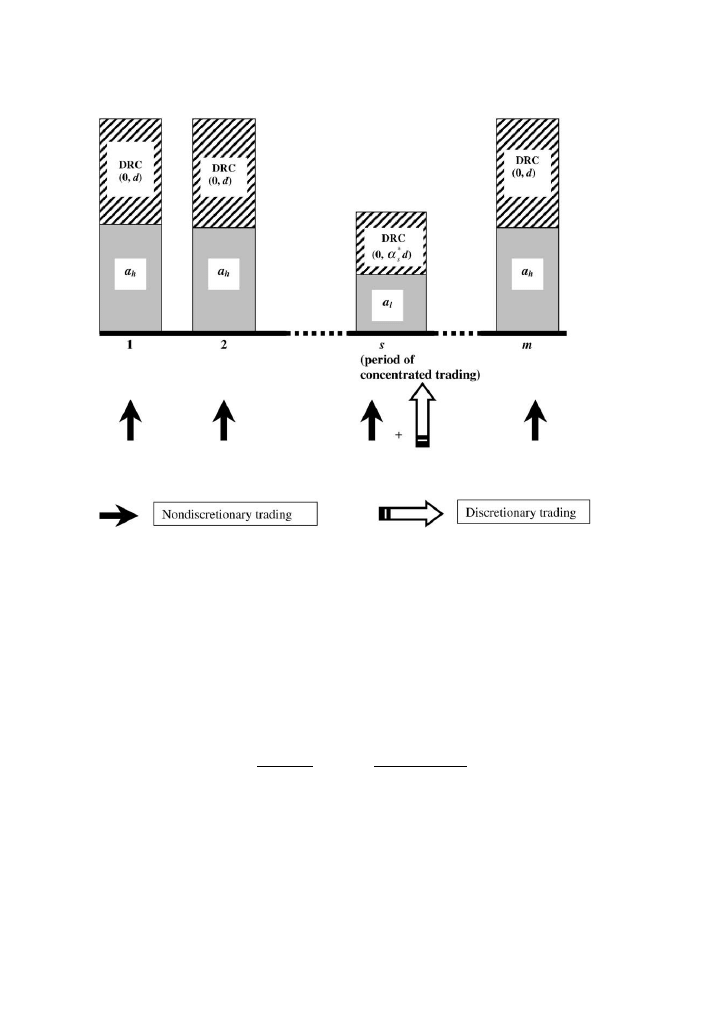
Fig. 2. A pictorial representation of the execution costs. The economy consists of m trading
periods. A fraction q

(endogenously determined) of the total number of liquidity traders (lT )

choose to act as discretionary traders and the remaining fraction (1 q

) prefer to act as

nondiscretionary traders. Before the market opens, discretionary traders choose optimal cutoﬀ level
a

o1) corresponding to each period t: They trade in the ﬁrst period that has discreteness

related commissions ðDRCÞ

; where d is the tick size. If the period of concentrated trading

occurs in Period s, DRC vary over (0, a

) and the adverse selection related commission is equal to

: In the remaining (m1) regular periods, the adverse selection related commission is equal to a

and DRC varies over the interval (0, d).

V.R. Anshuman, A. Kalay / Journal of Financial Markets 5 (2002) 83–125

100

in (m 1) periods of regular trading, given that DRC are, on average, equal to
d

/2. We explicitly factor in the depth of the market by including the number of

nondiscretionary traders (T

) incurring these commissions. Similarly, the

second term reﬂects the expected (per dollar) execution costs incurred by
liquidity traders in the period of concentrated trading. Finally, the last term
shows the cumulative monitoring costs incurred by all liquidity traders who act
as discretionary traders. It can be shown (see Appendix C) that the integration
of l TCðqÞ over the interval (0; q

) gives the expression: f lT Gððw 1Þ=wÞÞ

f1 GAMMADIST ½ðLnðq

Þg; where Gð:Þ is the gamma function and

GAMMADIST

is the cumulative distribution function of the standard gamma

distribution with parameter ½ðw 1Þ=w:

The expressions in the square bracket are normalized by the base price (P

This normalization is required to remove any spurious price eﬀects. Thus, our
objective function is expressed on a per dollar basis. This (inverse) measure of
liquidity reﬂects both the spread (i.e., commission) and the depth in the market.
Note, in Eq. (12) the base price appears explicitly in the denominator, and
implicitly in a

; a

; T

(through q

which depends on P

4. Numerical solution of the model

The model cannot be solved in closed-form. Therefore, we numerically solve

the model for reasonable parameter values. The numerical solution set
fa

;y; a

; q

; a

; P

g is used to compute the value of the transaction cost

function TCðP

Þ: Repeating this exercise for diﬀerent values of P

generates the

functional form of TCðP

Þ: The optimal base price is the one that results in the

lowest transaction cost.

4.1. The optimal cutoﬀs

The ﬁrst step in the numerical solution procedure is to solve Eq. (6) to

determine the optimal cutoﬀs, a

;y; a

: For these computations, we let the

number of trading periods (m) equal 10, the volatility parameter (k) equal 0.02,
and the tick size equal $0.125. A value of k ¼ 0:02 implies a standard deviation
of 2% (of the price level), which is consistent with observed daily standard
deviations.

Appendix B develops the functional form of the conditional

distribution, F

ða

j DRC

¼ z

dÞ

; and the expectation, Efz

d j z

;

DRC

¼ z

: These terms appear in Eq. (6). Table 2 shows the optimal

cutoﬀs at diﬀerent base prices varying from $1/2 to $100. The optimal cutoﬀs

Typical values of volatility of stocks lie in the range of 20–40% per annum, or equivalently

1.046–2.093% on a daily basis. Thus our choice of the parameter value is consistent with the daily
standard deviations observed on stock exchanges.

V.R. Anshuman, A. Kalay / Journal of Financial Markets 5 (2002) 83–125

101

depend on the base price because s

(the variance of d) depends on the base

price (s ¼ kP

Consider the case when the base price is $50. The cutoﬀ for the ﬁrst period is

0.1502. This means that discretionary traders would ﬁnd it optimal to trade in
the ﬁrst period only if the realized DRC in Period 1 is less than or equal to
0.1502d=$0.01877 (assuming a tick size of $0.125). Otherwise, they would
defer their trades to the next period. The last period cutoﬀ is always 1, since
discretionary are constrained to trade within the trading horizon (m=10
periods). It turns out that the optimal cutoﬀs are not very sensitive to the base
price, except at the very low base price of about $1.

Next, we apply the optimal cutoﬀs to Eq. (7) and determine discretionary

traders’ ex-ante expected DRC at each base price. This computation appears in the
bottom row of Table 2. For a base price of $50, the E(DRC)

=$0.0174, which is

signiﬁcantly lower than the nondiscretionary trader’s expected DRC of $0.0625.

4.2. The transaction cost function, TC(P

)

To construct the transaction cost function, we must ﬁrst solve for the

remaining endogenous variables in the solution set, namely, q

; a

; and a

;

corresponding to each base price level (P

). For convenience, we assume that

Table 2
The optimal cutoﬀs

This table shows the optimal cutoﬀs (a

) and discretionary traders’ ex-ante expected discreteness

related commissions [E(DRC)

] using a dynamic optimization procedure. The problem has been

solved for m=10 periods for diﬀerent base prices (P

). The base price level aﬀects the standard

deviation of the private information (s =kP

), where k is the volatility parameter. The m distinct

cutoﬀs (expressed as a fraction of the tick size) appear in the rows. We assume that the volatility
parameter (k) is equal to 0.02 and the tick size (d) is equal to $0.125.

Cutoﬀ (a

)

Base price (P

)

$1/2

$10

$50

$100

0.3839

0.1536

0.1492

0.1502

0.1499

0.4020

0.1763

0.1629

0.1636

0.1635

0.1631

0.4176

0.2099

0.1798

0.1797

0.1792

0.4318

0.2629

0.2011

0.1996

0.1992

0.4450

0.3281

0.2291

0.2249

0.2246

0.4579

0.3842

0.2675

0.2583

0.2581

0.4708

0.4285

0.3224

0.3047

0.3046

0.4843

0.4653

0.4000

0.3750

0.5000

1.0000

E(DRC)

0.0256

0.0183

0.0174

V.R. Anshuman, A. Kalay / Journal of Financial Markets 5 (2002) 83–125

102

the total trading population (T ) is equal to 200 (the results are invariant to the
choice of T ) and that the fraction of liquidity traders (l) is equal to 60% or 0.6.
The other key parameters are the monitoring cost parameters (f and w). They
deﬁne the shape of the monitoring cost schedule faced by liquidity traders. We
solve for q; a

; and a

; at diﬀerent base prices (P

) using the following

parameter values: d=$0.125, k=2%, m=10, T =200, l=0.6, and ðf ; wÞ
ð0:0109; 1:6Þ: We ﬁnd that the resulting transaction cost function, TCðP

Þ;

exhibits a local interior minimum at a base price of $53.

Table 3 presents the numerical solutions. Given l ¼ 0:6; the number of

uninformed liquidity traders (lT ) is equal to 120 and the remaining traders are
informed traders (80). Consider a base price of $10, as shown in the fourth row
of Table 3. First, the fraction of discretionary trading (q) is equal to 0.7169
(fourth column), which implies that 72% of the 120 liquidity traders act as

Table 3
Equilibrium characteristics

This table shows the numerical solution of the model at diﬀerent base prices. P

base price,

fraction of liquidity traders who choose to act as discretionary traders, a

adverse selection

related commissions in a regular period, a

adverse selection related commissions in the period of

concentrated trading, T

number of discretionary traders, and T

number of nondiscre-

tionary traders in each period. We assume that, in a continuum of increasing costs, the qth
percentile liquidity traders faces a monitoring cost, C(q)=f/[ln(q)]

1/w

, where f>0 and w>1. The

parameters deﬁning the numerical solution are as follows: (i) l: the fraction of liquidity traders in
the trading population (T), (ii) k: the volatility parameter, which speciﬁes the standard deviation of
the private information (d) in s(P

)=kP

, where P

is the base price, (iii) m: the number of periods,

(iv) d: the tick size, and (v) ( f, w): the monitoring cost parameter pair that deﬁnes the monitoring
cost schedule. The parameters chosen for the simulation are (i) l=0.6, T=200, (ii) k=0.02,
(iii) m=10, (iv) d=$0.125, and (v) f=0.0109, w=1.6.

0.5

0.0398

0.0042

0.9709

116.51

0.35

0.0362

0.0042

0.9486

113.83

0.62

0.0319

0.0044

0.9020

108.25

1.18

0.0247

0.0051

0.7169

86.03

3.40

0.0227

0.0055

0.6258

75.10

4.49

0.0218

0.0058

0.5745

68.94

5.11

0.0213

0.0061

0.5389

64.67

5.53

0.0209

0.0062

0.5115

61.37

5.86

0.0208

0.0063

0.5066

60.79

5.92

0.0208

0.0063

0.5042

60.50

5.95

0.0208

0.0063

0.5019

60.22

5.98

0.0206

0.0064

0.4885

58.62

6.14

0.0203

0.0066

0.4680

56.16

6.38

0.0200

0.0067

0.4485

53.82

6.62

0.0198

0.0069

0.4283

51.39

6.86

100

0.0189

0.0077

0.3453

41.43

7.86

V.R. Anshuman, A. Kalay / Journal of Financial Markets 5 (2002) 83–125

103

discretionary traders (=86.03, as shown in the ﬁfth column) while the
remaining 28% act as nondiscretionary traders.

Therefore, in each one of the

(=10) periods, 2.8% (=3.40, as shown in the last column) act as

nondiscretionary liquidity traders. The (per dollar) adverse selection commis-
sion in the period of concentrated trading is 0.0051 (third column) whereas the
(per dollar) adverse selection commission in the other nine periods is 0.0247
(second column).

In contrast, if the base price is equal to $100, as shown in the last row of

the table, a smaller fraction of the liquidity traders act as discretionary
traders (q

=35%). The (per dollar) adverse selection commission is 0.0077

in the period of concentrated trading and 0.0189 in the remaining regular
periods.

Besides adverse selection commissions, liquidity traders also incur DRC of

$0.0625, on average, in a regular period and much lower DRC (as shown in the
last row of Table 2) in the period of concentrated trading. Finally,
discretionary liquidity traders also incur monitoring costs. The total per
dollar expected transaction costs (incurred by all liquidity traders) can be
computed for a given base price (P

), as shown in Eq. (12). Table 4 shows

the total equilibrium expected transaction costs (last column) at various base
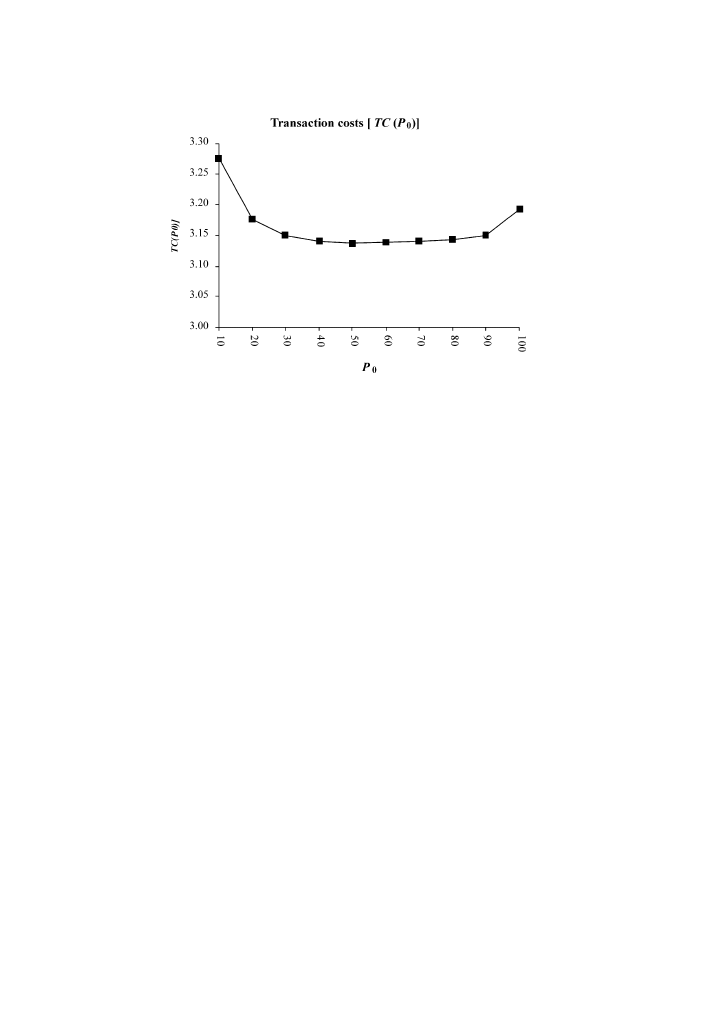
prices and Fig. 3 graphs the transaction costs as they vary with the base
price.

It can be seen both from Table 4 and Fig. 3 that the transaction cost function

½TCðP

Þ can be minimized by choosing an appropriate base price (P

). In this

case, the optimal base price is $53 and the (per-dollar) transaction costs
incurred at this base price are 3.1373. In contrast, had the base price been $100
(last row), the (per dollar) transaction cost would have been 3.1923. This
translates into a saving of 1.75%.

We are also interested in ﬁnding out whether the optimal price is

a global minimum or not. As the base price increases above $53, the
transaction cost function increases monotonically. No feasible solution
exists beyond a base price of $100. Therefore, the minimum at $53 is
a global minimum. In general, one cannot be sure whether the optimal
price is a global minimum or not because we are employing numerical

For convenience, we allow for fractional number of liquidity traders.

It might seem as if there is not much diﬀerence in transaction costs at the optimal price level of

$53, where TC(P

)=3.1373, and a high price level of $100, where TC(P

)=3.1923. Note that the

expected transaction cost is a per dollar measure. This implies that an investment of $100 when the
base price is $53 results in an absolute cost of 3.1373 100=$313.73. In contrast, had the base
price been $100, the absolute transaction costs would have been 3.1923 100=$319.23. Thus,
holding the base price at $53 results in a saving of $5.50 (=1.75% of $313.73) for 120 liquidity
traders.

V.R. Anshuman, A. Kalay / Journal of Financial Markets 5 (2002) 83–125

104

techniques to solve the model. However, given an upper bound on the
feasible set of prices that a ﬁrm can consider, even a local minimum over a
reasonable range of prices would suﬃce.

Table 4
Optimal price tradeoﬀs

This table shows total (expected) transaction costs incurred by all liquidity traders as a function of

the base price. P

base price, q fraction of liquidity traders who choose to act as discretionary

traders, a

adverse selection related commissions in a regular period, a

adverse selection related

commissions in the period of concentrated trading, T

number of discretionary traders, and

number of nondiscretionary traders in each period. We assume that, in a continuum of

increasing costs, the qth percentile liquidity traders faces a monitoring cost, C(q)=f/[ln(q)]

1/w

where f>0 and w>1. The parameters deﬁning the numerical solution are as follows: (i) l: the
fraction of liquidity traders in the trading population (T), (ii) k: the volatility parameter, which
speciﬁes the standard deviation of the private information (d) in s(P

)=kP

, where P

is the base

price, (iii) m: the number of periods, (iv) d: the tick size, and (v) ( f, w): the monitoring cost
parameter pair that deﬁnes the monitoring cost schedule. The parameters chosen for the simulation
are (i) l=0.6, T=200, (ii) k=0.02, (iii) m=10, (iv) d=$0.125, and (v) f=0.0109, w=1.6.

(Per dollar) expected transaction cost components

Base price (P

) Adverse

selection

Discreteness
related

Monitoring
cost

Total (per dollar)
transaction costs

0.5

0.6109

6.3778

2.3976

9.3864

0.6844

2.4413

2.2569

5.3826

0.8163

1.2813

2.0725

4.1701

1.2093

0.3463

1.7195

3.2752

1.3597

0.1954

1.6207

3.1757

1.4357

0.1386

1.5751

3.1494

1.4850

0.1083

1.5469

3.1402

1.5215

0.0893

1.5267

3.1375

1.5278

0.0863

1.5232

3.1374

1.5309

0.0849

1.5215

3.1373

1.5339

0.0836

1.5199

3.1374

1.5509

0.0763

1.5107

3.1379

1.5762

0.0668

1.4971

3.1402

1.5996

0.0596

1.4848

3.1441

1.6233

0.0541

1.4725

3.1499

100

1.7123

0.0528

1.4272

3.1923

Our only concern is that the global minimum could be a corner solution because TC(P

) may

go to 0 when P

approaches inﬁnity. We have two comments to make. First the stock price level is

bounded by the economic value of the ﬁrm (there must be at least one share), which rules out
inﬁnite values for P

. Second, note that if market makers are risk averse or face wealth constraints,

the breakeven commission charged by the market maker would increase at a faster rate than
predicted by our model, which has risk neutral market makers. In such a setting, TC(P

) would not

go to zero as P

approaches inﬁnity, and an interior global optimum would be realized. We can,

therefore, focus on the local minimum and interpret our model under the restriction that the base
price has to be less than some upper bound.

V.R. Anshuman, A. Kalay / Journal of Financial Markets 5 (2002) 83–125

105

4.3. Tradeoﬀs in the optimal price

The key feature of the model is that the base price (P

) aﬀects the economic

signiﬁcance of savings in execution costs accruing to potential discretionary
traders. While the base price does not aﬀect the (per dollar) adverse selection
commissions, it reduces the economic signiﬁcance of the ﬁxed cost component
– discreteness related commissions. Thus, (per dollar) execution costs depend
on the base price (P

). And, therefore, the amount of discretionary trading (q

)

depends on the base price (P

). At lower base prices, there is greater

discretionary trading because of the economic signiﬁcance of DRC. Con-
versely, there is lesser discretionary trading at higher base prices. This
dependence of the distribution of trades (across time) on the base price, in turn,
aﬀects total transaction costs incurred by traders across all the periods. In
other words, total transaction costs depend on the base price (P

To get a better insight of the tradeoﬀs in the optimal price, we rearrange

the ﬁrst two terms of the transaction cost function described in Eq. (12) as
follows:

TCðP

Þ ¼ ½ðm 1Þa

þ a

ðT

þ T

Þ=P

þ ½ðm 1Þðd=2ÞT

þ EðDRCÞ

ðT

þ T

Þ=P

þ f ðlTÞGððw 1Þ=wÞf1 GAMMADIST ½Lnðq

Þg

ð13Þ

Fig. 3. The transaction costs function [TC(P

)] is shown as a function of the base price P

. The

transaction costs are made up of the sum of adverse selection related commissions and discreteness
related commissions incurred by all liquidity traders in all periods as well as the (cumulative)
monitoring costs incurred by all discretionary liquidity traders. At a base price of approximately
$53, the transaction costs are minimized.

V.R. Anshuman, A. Kalay / Journal of Financial Markets 5 (2002) 83–125

106

¼ sum of adverse selection commissions in m periods

þ sum of DRC in m periods

þ ðcummulativeÞ monitoring costs:

TCðP

Þ; as described in Eq. (13) consists of three terms expressed in per

dollar amounts. The ﬁrst term is the sum total of (per dollar) adverse selection
commissions paid by all liquidity traders in all m periods (for clarity, we refer
to the sum total of adverse selection commissions as the adverse selection
component

). The second term is the sum total of (per dollar) DRC incurred by

all liquidity traders in all m periods (again, for clarity, we refer to this as the
DRC component

). Finally, the third term indicates the (cumulative) monitoring

costs incurred by discretionary liquidity traders (see Appendix C for a
derivation of the monitoring cost component).

Table 4 shows the three components at diﬀerent base prices. It can be seen

(in the second column of Table 4) that the adverse selection component
increases as the base price increases, whereas the DRC component (third
column) and the monitoring cost component (fourth column) decrease with the
base price. The optimal base price of $53 strikes the right balance between
these components.

The result can be explained with the help of Table 3. As the base price

increases, fewer liquidity traders act as discretionary traders (q

is lower)

because the economic signiﬁcance of savings in DRC is lower. The reduction in
discretionary trading has the following eﬀects. First, adverse selection
commissions in the period of concentrated trading increase (third column in
Table 3). Second, fewer traders beneﬁt from trading in the period of
concentrated trading (ﬁfth column in Table 3). Third, more liquidity traders
trade in regular periods (last column in Table 3). Fourth, the adverse selection
commissions in the regular period decrease (second column in Table 3).
However, they are still higher than in the period of concentrated trading. The
net eﬀect is that the adverse selection component of TCðP

Þ increases with the

base price (P

Now consider the DRC component of TCðP

Þ: Less concentrated trading at

higher base prices implies that fewer liquidity traders incur the low DRC in the
period of concentrated trading. Also, more liquidity traders trade in the other
periods where DRC is, on average, higher. Therefore, both eﬀects work toward
increasing (dollar) DRC. However, (dollar) DRC does not increase as fast as
the base price and the (per dollar) DRC component decreases in the base price,
unlike the adverse selection component.

Finally, the monitoring cost component decreases with the price level

because there is less concentrated trading at higher price levels and fewer
liquidity traders incur monitoring costs. There exists a tradeoﬀ between an
increasing adverse selection cost component and decreasing DRC and

V.R. Anshuman, A. Kalay / Journal of Financial Markets 5 (2002) 83–125

107

monitoring cost components of the transaction cost function. This tradeoﬀ
results in an interior optimum.

The intuition of the model can also be explained as follows. A lower base

price induces more liquidity traders to act as discretionary traders. This is
beneﬁcial because greater discretionary trading results in a lower adverse
selection component. However, a lower base price also has adverse cost
implications. First, the DRC component increases and higher (cumulative)
monitoring costs are incurred because more liquidity traders act as
discretionary traders. The optimal price, which results in an optimal amount
of discretionary trading, is the one equating the marginal adverse selection
component on the one hand to the sum of the marginal DRC and the marginal
monitoring components on the other hand.

4.4. Robustness checks

To check the robustness of our results, we numerically solved the model for

various parameter values.

The basic parameters are the liquidity parameter

(l), the volatility parameter (k), the trading horizon (m), and the tick size (d).
Given speciﬁc values for l; k; m; and d; we ﬁnd that the existence of an interior
local optimum of the transaction cost function depends on monitoring cost
parameter pair ( f ; w). We show that by appropriately choosing values for
( f ; w), one can demonstrate the existence of an interior (local) optimal price
for a wide range of reasonable parameter values for fl; k; m; dg:

The results are presented in Table 5. In Panel A of Table 5, we consider two

polar cases of the liquidity parameter (l). Consider the case where l ¼ 0:1: By
appropriately choosing ðf ; wÞ ð0:0119; 2:1Þ; we show the existence of an
optimal price ($32) when l is as low as 0.1. On the other hand, by choosing
ðf ; wÞ ð0:0065; 2:2Þ; an optimal price exists ($71) when l is as high as 0.9.

A ﬁnal point is in order. At ﬁrst glance, it might seem that the results of our model could be

obtained by explicitly introducing the asset price level and endogenizing discretionary trading in the
Admati and Pﬂeiderer (1989) model. However, our model has an additional feature – price
discreteness. The exchange-mandated discrete pricing restriction plays an important role in our
model. To see this, observe Eq. (10) that describes the savings in execution costs. Note that in the
absence of discrete prices, savings in executions costs arise purely because of savings in adverse
selection commissions, ½ða

Þ=P

; and not because of savings in DRC, ½d=2 EðDRCÞ

: As

shown in Appendix A, the saving, ½ða

Þ=P

; is independent of the price level. Therefore, q

;

which is a function of the savings, is independent of the base price in this set up [see Eq. (11)]. As a
consequence, in a model without discrete prices, the total transaction cost function would be
independent of the price level. Unlike our model, there would be no optimal price.

We ﬁnd that, for some parameter sets, there exist multiple solutions for the endogenous

variables (a

; a

; and q

), depending on the initial seed values. To obtain the results in the paper, use

initial seed values close to the given solution of a

and a

For some parameter sets, the transaction cost function, TCðP

Þ; is monotonically decreasing in

, and no interior optimal price exists.

V.R. Anshuman, A. Kalay / Journal of Financial Markets 5 (2002) 83–125

108

Similarly, in Panel B of Table 5, we demonstrate the existence of an optimal
price for two polar cases of the volatility parameter. For k=0.2%, we let
ðf ; wÞ ð0:0015; 1:5Þ and show that an optimal price exists ($98). For k=2%,
we let ðf ; wÞ ð0:0105; 1:6Þ and show that the optimal price is $120. Panel C of
Table 5 shows how the optimal price changes as the trading horizon (m)
increases from 10 to 11. We ﬁnd that the optimal price increases with the
trading horizon. Finally, we demonstrate the interior optimal price for two
diﬀerent tick size regimes in Panel D of Table 5.

4.5. Optimal price behavior

Fig. 4 illustrates the results of numerical solutions. Panel A shows that the

optimal price is increasing in the volatility parameter (k). Panels B, C, and D
show that the optimal price is decreasing in the liquidity parameter (l), and the
monitoring cost parameters, f and w; respectively. Finally, Panel E shows that
the optimal price is increasing in the tick size (d).

The relationship between the optimal price and the tick size is linear. Table 6

shows the optimal price for diﬀerent tick sizes and the consequent eﬀective tick

Table 5
Robustness checks

This table presents the optimal base price for diﬀerent parameter values. We assume that, in a

continuum of increasing costs, the qth percentile liquidity traders faces a monitoring cost, C(q)
=f/[ln(q)]

1/w

, where f>0 and w>1. The parameters deﬁning the numerical solution are as

follows: (i) l: the fraction of liquidity traders in the trading population (T), (ii) k: the volatility
parameter, which speciﬁes the standard deviation of the private information (d) in s(P

)=kP

where P

is the base price, (iii) m: the number of periods, (iv) d: the tick size, and (v) ( f, w): the

monitoring cost parameter pair that deﬁnes the monitoring cost schedule. T is assumed to be equal
to 200 in all cases.

Panel A. Liquidity parameter

(l)

l=0.1

ð f ; wÞ ð0:0119; 2:1Þ

ðm; k; dÞ ð10; 0:02; 0:125Þ

=32

l=0.9

ð f ; wÞ ð0:0065; 2:2Þ

ðm; k; dÞ ð10; 0:02; 0:125Þ

=71

Panel B. Volatility parameter

(k)

=0.002

ð f ; wÞ ð0:0015; 1:5Þ

ðm; l; dÞ ð10; 0:60; 0:125Þ

=98

=0.02

ð f ; wÞ ð0:0105; 1:6Þ

ðm; l; dÞ ð10; 0:60; 0:125Þ

=120

Panel C. Trading horizon

(m)

=10

ð f ; wÞ ð0:0105; 1:6Þ

ðl; k; dÞ ð0:70; 0:02; 0:125Þ

=35

=11

ð f ; wÞ ð0:0105; 1:6Þ

ðl; k; dÞ ð0:70; 0:02; 0:125Þ

=72

Panel D. Tick size

(d)

=$0.0625

ð f ; wÞ ð0:0105; 1:6Þ

ðm; k; lÞ ð10; 0:02; 0:60Þ

=60

=$0.125

ð f ; wÞ ð0:0105; 1:6Þ

ðm; k; lÞ ð10; 0:02; 0:60Þ

=120

V.R. Anshuman, A. Kalay / Journal of Financial Markets 5 (2002) 83–125

109

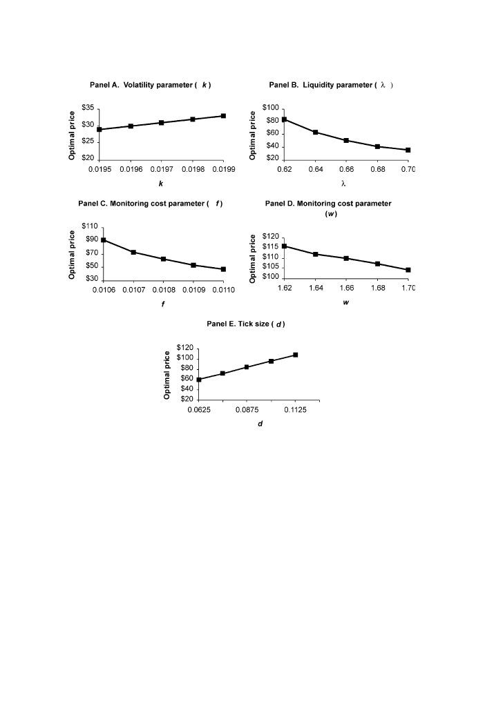
size (ratio of tick size to price). It can be seen that the eﬀective tick size stays the
same in all cases. In other words, given a set of parameters (other than the tick
size), there exists an optimal eﬀective tick size that minimizes transaction costs.
As the tick size changes, the optimal price also changes proportionately,
resulting in the same eﬀective tick size.

What really matters is the eﬀective tick size. In the U.S., because the tick size

is ﬁxed across all price levels (barring stock prices below $1), the optimal
eﬀective tick size can be transformed into an equivalent optimal price level.
Furthermore, one can also interpret this model in terms of an optimal amount

Fig. 4. The optimal price behavior. Panels A–E describe how the optimal price changes as one of
the exogenous parameter changes in value. The optimal price is increasing in the volatility
parameter (k), decreasing in the liquidity parameter (l), monitoring cost parameters ( f, w), and
increasing in the tick size (d). Note that the relationship between the optimal price and the tick size
is linear.

V.R. Anshuman, A. Kalay / Journal of Financial Markets 5 (2002) 83–125

110

of discretionary trading (q

The optimal eﬀective tick size induces an

optimal amount of discretionary trading. The last two columns show that the
equilibrium amount of discretionary trading (q

) and the minimized transac-

tion cost (at the optimal price) are the same for all cases.

5. Empirical implications and evidence

Our theory is consistent with existing empirical evidence but it also

leads to new empirical implications. We contrast the predictions of our
theory with the predictions of the popular hypothesis, which states that splits
allow a larger set of stockholders to buy round lots, thereby lowering the
commissions paid and thus increasing the ﬁrms’ stockholders base. We start by
presenting empirical evidence consistent with both our theory and the popular
hypothesis. We then present empirical evidence consistent with our model,
but inconsistent with the popular hypothesis. Table 7 presents a list of
empirical implications of our model and the popular hypothesis and the related
evidence.

Table 6
Tick size and optimal price

This table shows the optimal price behavior as the tick size changes. P

base price, q

fraction

of liquidity traders who choose to act as discretionary traders. We assume that, in a continuum of
increasing costs, the qth percentile liquidity traders faces a monitoring cost, C(q)=f/[ln(q)]

1/w

)=kP

, where P

is the base

price, (iii) m: the number of periods, (iv) d: the tick size, and (v) ( f, w): the monitoring cost
parameter pair that deﬁnes the monitoring cost schedule. The parameters chosen for the simulation
are: (i) l=0.6, T=200, (ii) k=0.02, (iii) m=10, and (iv) f=0.0105, w=1.6.

Tick
size (d)

Optimal
price (P

)

Optimal
eﬀective tick (d/P

)

Optimal amount
of discretionary
trading (q*)

Total (per dollar)
minimized
transaction
cost [TC(P

)]

0.0625

0.0010

0.5183

3.0249

0.0750

0.0010

0.5183

3.0249

0.0875

0.0010

0.5183

3.0249

0.1000

0.0010

0.5183

3.0249

0.1125

108

0.0010

0.5183

3.0249

Although q

is endogenously determined, it is not a choice variable like the tick size or the base

price.

V.R. Anshuman, A. Kalay / Journal of Financial Markets 5 (2002) 83–125

111

5.1. Evidence consistent with our model and the popular hypothesis

Our model and the popular hypothesis predict that, other things constant,

signiﬁcant increases in stock price should precede stock splits. Both the theory and
the hypothesis imply that announcements of splits would lead to positive stock
market response.

Empirical evidence consistent with this implication has been

documented in Fama et al. (1969). Positive announcement eﬀects are documented
in Grinblatt et al. (1984), and Eades et al. (1984). We turn now to present evidence
consistent with our model and unrelated to the popular hypothesis.

5.2. Stock distributions and the minimum tick size

The pattern of stock distributions varies signiﬁcantly between the U.S. and

Japan. Relative to Japanese ﬁrms, U.S. corporate managers seem to split their

Table 7
Empirical implications

This table presents a list of empirical implications and corresponding evidence of our theory and

the popular hypothesis of stock splits.

Empirical implications

Our theory

Popular
hypothesis

Evidence

Stock price before the split

Increase

Increase (Fama et al., 1969)

Announcement eﬀects

Positive

Positive (Grinblatt et al., 1984)

Price level in U.S.

Constant

Constant (Angel, 1997)

Frequency of splits in Japan

(relative to U.S.)

Lower

The same

Lower (Section 5.2)

Price level in Japan

Increase
with time

Constant

Increase with time
(Section 5.3)

Concentration of

trades and price level

Negative
relationship
is possible

No relationship

Negative relationship
(Section 5.4)

Concentration of trades

after a split

Higher

The same

Higher (Anshuman and
Goyal, 2001)

Stock return variability

Higher

The same

Higher (Ohlson and
Penman, 1985)

The popular hypothesis states that ﬁrms split their stocks to enable investors with binding

wealth constraints to buy round lots; thereby reducing their transaction costs. By doing that the
ﬁrm increases its stockholders’ base.

Note, this conclusion depends on the extent to which the market is surprised by the ﬁrm’s

decision to split. This situation can arise if (i) the ﬁrm is more knowledgeable about the
composition of liquidity traders, (ii) the ﬁrm has a better estimate of the costs of implementing a
split, and (iii) the ﬁrm (as compared to the market) can better anticipate changes in the premium
associated with its own stock’s liquidity. Under such circumstances, market participants would not
be able to predict with certainty the timing or the magnitude of the split.

V.R. Anshuman, A. Kalay / Journal of Financial Markets 5 (2002) 83–125

112

stocks much more frequently. Our model can help explain this puzzling
diﬀerence by examining the minimum price variation rules in Japan. The
minimum tick size is constant only over a range of stock prices and increases as
the level of the stock price increases. For instance, the tick size is 1 yen for
stock prices up to 2000 yen, 5 yen for stock prices in the 2000–3000 yen range,
10 yen for stock prices in the 3000–30,000 yen range, 50 yen for stock prices in
the 30,000–50,000 yen range, and so on. The eﬀective tick size varies over the
interval (0.0003, 0.0100) over all price levels. In contrast to the U.S., the
eﬀective tick size stays bounded within an interval and does not monotonically
decrease with the stock price level. Our theory predicts that Japanese ﬁrms can
allow the stock price level to drift without being too concerned about moving
too far away from an optimal eﬀective tick size. Unlike the U.S., Japanese
ﬁrms need not maintain constant nominal prices. We, therefore, expect them to
split their stocks less frequently than U.S. ﬁrms.

Fig. 5 (Panel A) displays the relative occurrence of stock dividends and splits

in the U.S. during the period 1985–1999. The data used in this ﬁgure has been
derived from the NYSE Fact Book (1994, 1999). There were a total of 2644
distributions during this period. Among these distributions, there were 362
(about 14%) distributions of size less than 25% whereas 2282 (about 86%)
distributions qualiﬁed as stock splits. 1399 (about 53%) of the distributions
were of size greater than 100%. During this period, U.S. ﬁrms have employed a
greater proportion of stock splits as compared to stock dividends.

Fig. 5 (Panel B) presents similar information for the Japanese stock markets

during the eight-year period 1983–1990. There were approximately 2982 stock
distributions. Interestingly, the average split factor is only 17% (the minimum
is 1%, and the maximum is 50%). There were 2799 distributions (about 94%)
of size less than 25% and zero distributions of size greater than 100%. More
importantly, only 183 distributions (about 6%) fell under the category of stock
splits. In Japan, stock dividends seem to be much more prevalent than stock
splits.

5.3. Average stock price

Because the tick size is ﬁxed in nominal terms at $0.125, U.S. ﬁrms wishing

to maintain a constant optimal (eﬀective) tick size must keep their nominal
stock price constant. Splits and reverse splits can be used to achieve this
outcome. Indeed the empirical evidence indicates that, in spite of inﬂation,
positive real interest rates, and signiﬁcant risk premiums, the average nominal
stock price in the U.S. during the last 50 years has been almost constant. Angel
(1997) presents empirical evidence, which shows that the average share price on

One must also note that institutional diﬀerences between the U.S. and Japan regarding stock

distributions might provide an alternative explanation of the results reported here.

V.R. Anshuman, A. Kalay / Journal of Financial Markets 5 (2002) 83–125

113

the NYSE has changed from $39.86 in 1951 to $37.27 in 1991. The average
share price on the NYSE has mostly hovered very close to the $40 mark during
the period 1951–1991.

As mentioned above, Japanese ﬁrms, in contrast, can maintain a long-run

stable eﬀective tick size even in the presence of rapid stock price increases.
Thus, Japanese ﬁrms need not maintain constant nominal stock prices to attain
their optimal eﬀective tick size. In the presence of positive inﬂation, real
interest rates, and positive risk premiums, one should expect to see a rising
trend in the average stock price over an extended period of time. The evidence
on the distribution of stock prices on the ﬁrst section of the Tokyo Stock
Exchange over the period 1950–1990 is consistent with this prediction. Ide
(1994) reports that the percentage of stocks with market value less than 500 yen
has decreased from 99% in 1950 to about 8% in 1990. During the same period
the percentage of stocks between 1000 and 2000 yen has risen from zero to 31%
and the percentage of stocks above 2000 yen has increased from zero to 17%.

Fig. 5. Stock distributions in the U.S. and Japan. Panels A and B show the histogram of stock
distributions in the U.S. (1985–1999) and Japan (1983–1990), respectively. The proportion of stock
splits to stock dividends in Japan is much lower than in the U.S. [Source: Panel A has been
constructed from data appearing in NYSE Fact Book (1994, 1999) and Panel B has been
constructed from data appearing in Ide (1994).]

V.R. Anshuman, A. Kalay / Journal of Financial Markets 5 (2002) 83–125

114

This rising trend is also apparent from the increase in the average share price
from 74 yen in 1950 to 1577.50 yen in 1990.

5.4. Coeﬃcient of variation of per period trading volume and price levels

Our model implies that diﬀerent ﬁrms would maintain their stock at diﬀerent

optimal levels depending on the relevant values of the parameter set
fl; k; m; d; f ; wg: Interestingly, an optimal price is also associated with an
equilibrium amount of discretionary trading (q

). Therefore, diﬀerent ﬁrms

(preferring diﬀerent optimal prices) would experience diﬀering degrees of
discretionary trading (or concentrated trading), depending on their parameter
values.

In this section we empirically examine the cross-sectional relationship

between price levels of ﬁrms and the degree of concentrated trading in their
stock. For this purpose, we study a sample of intraday transaction data for
2173 stocks trading on the NYSE during August 1993. The raw data consist of
time-stamped transactions as well as quote data obtained from the TAQ data
set. For transactions, price and volume data are available, while for quotes, bid
and ask quotes are available. To allow for a homogenous market regime, the
opening and closing sessions of trading have not been used in our empirical
tests. Thus, the sample consists of data from 22 trading days between
10:00 a.m. and 4:00 p.m.

For each stock, we computed the average transaction price (PRICE) based

on all transactions for that stock in the 22-day trading period. PRICE
represents the stock price level. For the entire sample of stocks, PRICE had a
mean of $27.90, a minimum value of $0.091825, and a maximum value of
$6830.49.

For our sample data on the NYSE, the tick size is equal to $1/16 for stocks

trading between $0.25 and $1.00, and further reduces to $1/32 for stocks priced
below $0.25. We excluded transaction data for all stocks that had PRICE less
than or equal to one dollar in order to restrict our test to a single tick size.
Furthermore, we also excluded all stocks that had less than (or equal to) 100
transactions over the entire sample period. After these exclusions, our ﬁnal
sample had 1796 stocks.

For each stock in the sample, we aggregated trading volume over 5-, 15-, 30-,

and 60-minute intervals. Over 22 trading days, aggregation of 5-minute trading
volume results in 1584 observations (22 days 6 hours 12 5-minute intervals)
for each stock. Similarly, each stock has 528 15-minute trading volume
observations, 264 30-minute observations, and 132 60-minute observations.

VSTD

denotes the standard deviation of the volume series of a stock. We ran

a regression of VSTD on PRICE. Because VSTD may be higher for stocks with
higher average trading volume, we added VMEAN as an independent variable
in the regression, where VMEAN is the mean of the aggregated volume of the

V.R. Anshuman, A. Kalay / Journal of Financial Markets 5 (2002) 83–125

115

stock in question. The results of this regression are reported in Table 8. The
ﬁrst four columns show the results of the regression where volume is
aggregated every 5, 15, 30, and 60 minutes, respectively. The evidence presented
here indicates that volatility of aggregated volume is negatively related to the
price level. Higher priced stocks have a smoother volume of trade.

To check

for multicollinearity, we computed the correlation between PRICE and
VMEAN

and found it to be statistically insigniﬁcant. The Pearson correlation

is equal to 0.0439 (p-value=0.0406), which indicates that the regression
speciﬁcation does not suﬀer from multicollinearity.

Table 8 also presents results associated with an alternative proxy of the

degree of concentrated trading, the Herﬁndahl Index. It is computed as
follows. If V05

denotes the trading volume for a stock in a particular 5-minute

trading period i; and V05SUM denotes the total trading volume for that stock
over the entire sample period, then the Herﬁndahl Index (HERF) is given by
S

(V05

/V05SUM)

. The Herﬁndahl indices for 15-, 30-, and 60-minute

aggregated volume data are constructed in a similar manner. Table 8 shows
that the Herﬁndahl Index is (signiﬁcantly) negatively related to the stock price
level. These results imply that the volume series of higher priced stocks is
smoother than that of lower priced stocks.

Next we investigate whether an inverse relationship between price level and

the degree of concentrated trading is possible in the context of our model. To
measure the degree of concentrated trading, we note that the per period trading
volume in the m periods is not constant because the trading volume increases in
the period of concentrated trading. We can show that the mean and standard
deviation of per period (expected) trading volume is ½lT=m þ ð1 lÞT and
ð1=mÞ

0:5

½q

lT ; respectively.

It follows that the coeﬃcient of variation, which

is deﬁned as the ratio of the standard deviation to the mean, is given by

In an earlier version of the paper we used intraday transaction data from 42 trading days

during the months of March and April, 1985. We found very similar results to that reported in
Table 8.

The m trading periods can be classiﬁed into (m 1) regular periods and one period of

concentrated trading. In a regular period only nondiscretionary liquidity trading occurs along with
informed trading. In contrast, in the period of concentrated trading, both nondiscretionary and
discretionary liquidity trading occurs along with informed trading. The per period trading volume
is therefore not constant across all periods, as shown in Fig. 2. Trading volume in a regular period
is equal to ð1 q

ÞlT=m of nondiscretionary trades and ð1 lÞT of informed trades. In contrast,

trading volume in the period of concentrated trading is equal to q

lT of discretionary trades,

ð1 q

ÞlT=m of nondiscretionary trades, and ð1 lÞT of informed trades. The mean of per period

trading volume in (m 1) regular periods and one period of concentrated trading is given by
½ðm 1Þ=m½ð1 q

ÞlT=m þ ð1 lÞT þ ð1=mÞ ½q

lT þ ð1 q

ÞlT=m þ ð1 lÞT; which simpliﬁes

to ½lT =m þ ð1 lÞT: The variance of per period trading volume is given by ð1=ðm 1ÞÞ½ðm 1Þ
f½ð1 q

ÞlT=m þ ð1 lÞT ½lT=m þ ð1 lÞTg

þ f½q

lT þ ð1 q

ÞlT=m þ ð1 lÞT ½lT=m

þð1 lÞTg

; which simpliﬁes to ð1=mÞ ½q

: It follows that the standard deviation is ð1=mÞ

0:5

½q

lT and the coeﬃcient of per period trading volume is given by m

0:5

½q

l=½l þ ð1 lÞm:

V.R. Anshuman, A. Kalay / Journal of Financial Markets 5 (2002) 83–125

116

Table 8
Concentration of trading volume

This table shows the results of the following regressions:

VSTD ¼ a þ b PRICE þ c VMEAN

;

HERF ¼ a þ b PRICE þ c VMEAN

;

where VSTD ðtimeseriesÞ standard deviation of each stock’s volume aggregated over a 5 (15, 30, and 60) minute interval, PRICE average
transaction price of each stock over the entire sample period, VMEAN ðtimeseriesÞ mean of each stock’s volume aggregated over a 5 (15, 30, and 60)
minute interval, and HERF Herfindahl Index of the 5 (15, 30, and 60) minute volume series. The number of observations in all regressions is equal to
1796. Each cell contains the regression coeﬃcient, the t-statistic, and the p-value, respectively.

VSTD=a+bPRICE+cVMEAN

HERF=a+bPRICE+cVMEAN

(1) 5 min

(2) 15 min

(3) 30 min

(4) 60 min

(1) 5 min

(2) 15 min

(3) 30 min

(4) 60 min

0.6474

0.7255

0.7263

0.7172

0.0323

0.0404

0.0391

0.0361

INTERCEPT

4556.44

7602.27

10,076

5751.26

0.0306

0.0418

0.0577

0.0398

14.292

13.177

10.025

11.068

33.665

45.902

58.545

40.924

0.0001

PRICE

6.724

6.906

5.959

7.465

7.04E06

4.10E06

2.75E06

6.02E06

8.465

10.459

9.821

9.414

3.103

3.937

4.616

4.036

0.0001

0.0019

0.0001

VMEAN

1.122

0.8554

0.7480

1.101

2.71E07

7.84E08

2.96E08

1.17E07

53.069

58.936

57.688

59.444

4.489

3.422

2.331

3.367

0.0001

0.0006

0.0199

0.0008

V.R.

Anshuman

Kalay

Journal

of
Financial

Markets

(2002)

83–125

117

0:5

½q

l=½l þ ð1 lÞm: Note that both standard deviation and coeﬃcient of

variation are functions of q

; which depends on the entire parameter set

fl; k; m; d; f ; wg:

Table 9 shows a series of optimal prices and the associated coeﬃcient of

variation in per period trading volume. One can see that the optimal price
changes as the liquidity parameter (l) changes. Associated with each optimal
price are the amount of discretionary trading (q

), the standard deviation of per

period trading volume and the coeﬃcient of variation of per period trading
volume. There is an inverse relationship between the price level and the
standard deviation or the coeﬃcient of variation in volume. This implies that
our model is consistent with the empirically established negative relation
between price and concentrated trading reported in this section.

5.5. Post-split coeﬃcient of variation in trading volume

A stock split oﬀers a natural experiment to empirically test our model. After

a split, the only change that occurs is that of the price level. According to our
model, the lower price level after a split should cause an increase in the amount
of discretionary trading (q

). From the discussion in the previous section, we

can see that the standard deviation and coeﬃcient of variation of per period

Table 9
Concentration of trading volume and price level

This table shows that a negative relationship between the degree of concentrated trading and the

price level is possible in the context of the model. As l increases, the optimal price increases. In
contrast, the sample standard deviation and coeﬃcient of variation of per period trading volume
decrease with l. P

base price, q fraction of liquidity traders who choose to act as

discretionary traders. We assume that, in a continuum of increasing costs, the qth percentile
liquidity traders faces a monitoring cost, C(q)=f/[ln(q)]

1/w

, where f>0 and w>1. The parameters

deﬁning the numerical solution are as follows: (i) l: the fraction of liquidity traders in the trading
population (T), (ii) k: the volatility parameter, which speciﬁes the standard deviation of the private
information (d) in s(P

)=kP

, where P

is the base price, (iii) m: the number of periods, (iv) d: the

tick size, and (v) ( f, w): the monitoring cost parameter pair that deﬁnes the monitoring cost
schedule. The parameters chosen for the simulation are: (i) T=200, (ii) k=0.02, (iii) m=10, (iv)
d

=$0.125, and (v) f=0.0105, w=1.6.

Liquidity
parameter
(l)

Optimal
price
(P

Optimal
eﬀective
tick size
(d/P

Optimal amount
of discretionary
trading
(q*)

Standard
deviation
of per period
trading volume

Coeﬃcient of
variation
of per period
trading volume

0.70

0.0036

0.4543

404.44

0.2718

0.68

0.0030

0.4736

414.86

0.2625

0.64

0.0020

0.4985

407.12

0.2379

0.62

0.0015

0.5083

397.32

0.2255

0.60

120

0.0010

0.5183

386.79

0.2138

V.R. Anshuman, A. Kalay / Journal of Financial Markets 5 (2002) 83–125

118

trading volume are increasing in q

: Our model, therefore, implies that a stock

split should result in a higher standard deviation and coeﬃcient of variation of
per period trading volume. Anshuman and Goyal (2001) examine a sample of
stock splits during 1993–1994 and ﬁnd that, subsequent to stock splits, there is
an overall increase in the coeﬃcient of variation of trading volume aggregated
over short intervals. This result is consistent with our model’s prediction.

5.6. Post-split volatility of returns

Note that the periods of concentrated trading on the ask and bid sides of the

market, in general, do not coincide because DRC on the ask side and bid side
of the market are not identical.

Thus during periods of concentrated buying

(selling), the average transaction price is biased toward the ask (bid) price. This
bias causes signiﬁcant price changes across the period of concentrated trading,
thereby creating volatility. Given that there is greater amount of discretionary
trading after a split, the above eﬀect should be more pronounced after a split.
Our model implies that the volatility of returns should increase (decrease) after
a split (reverse split). Ohlson and Penman (1985), Lamoureux and Poon (1987),
and Koski (1998) present evidence that is consistent with this implication of the
model.

5.7. Decimalization of the minimum tick size

Our model suggests a linear relationship between the optimal price level and

the tick size. This result has implications for the proposed decimalization of
tick sizes on stock exchanges. If the tick size were to be reduced to 1 cent, the
optimal price would drop by a factor of 12.5, i.e., a $50 optimal price would
drop down to $4. This would mean that ﬁrms would undo the eﬀect of the
change in tick size by employing stock splits. According to our model, when
ﬁrms believe that the new tick size is going to persist, they would employ a
series of splits or a one-time large split to converge to lower trading range. This
is an experiment that time will make possible. We believe that it is too early to
interpret the current evidence (on stock split activity) either in favor of our
model or against it.

More importantly, we note that exchanges and regulating

bodies in the U.S. do not choose the eﬀective tick size. They never did. Firms

Asymmetric DRC on the ask and bid side arise because the true equilibrium price is, in general,

asymmetrically located with respect to feasible discrete prices. See Anshuman and Kalay (1998) for
a more detailed discussion of this issue.

As pointed out by Angel (1997), there was a switch in price quoting rules from percentage of

par to dollar pricing in 1915. With percentage of par pricing, the eﬀective tick size is invariant to the
price level and there were relatively few splits before 1915. After 1915, with dollar pricing, the
eﬀective tick size depended on the price level. However, it took about 14 years for the average stock
price on the NYSE to drop from about $90 to $40, thereby doubling the eﬀective tick size.

V.R. Anshuman, A. Kalay / Journal of Financial Markets 5 (2002) 83–125

119

choose the eﬀective tick size by splitting and reverse splitting the stocks. If we
believe that insiders in ﬁrms know better than us as to what a stock’s optimal
eﬀective tick size should be, any attempt to intervene via regulation is pointless.

6. Conclusion

This paper presents a theory that argues that splits improve liquidity. The

driving force behind the model is the discrete pricing restriction on organized
exchanges. Execution costs arising from discreteness vary over time. Liquidity
traders have an incentive to time their trades to lower their execution costs. The
asset price level aﬀects their incentives because discreteness related costs are
determined by a nominally ﬁxed tick size. By splitting, a ﬁrm lowers its stock
thereby increasing the incentives of liquidity traders to time their trades. The
resulting concentration of trades reduces overall transaction costs incurred by
liquidity traders. Our analysis also establishes the existence of an optimal price
level that minimizes transaction costs. Stock split factors can be adjusted to
reset the stock price level to the optimal level.

Appendix A. Derivation of Eq. (1)

The informed trader’s proﬁt conditional on observing d is equal to (d a),

where a is the ask commission charged by the market maker. The market
maker infers that the informed trader would trade only when d is greater than
a

: Therefore, he computes his expected losses to informed traders to be equal to

ð1 lÞT E½ðd aÞjd > a: At the same time his expected proﬁts from liquidity
traders is equal to ðlT =mÞa: Setting the market maker’s expected proﬁts to zero
yields the equilibrium commission (a

), i.e., a

is given by the solution of the

following equation:

ð1 lÞT Probfd > agE½ðd aÞjd > a þ ðlT=mÞa ¼ 0:

ðA:1Þ

The conditional expected value, E½ðdÞ j d > a; given d Nð0; sðP

Þ; is equal to

sðP

Þ ffða=sðP

ÞÞ=½1 Fða=sðP

Þg (see Johnson and Kotz, p. 81), and noting

that Probfd > ag ¼ ½1 Fða=sðP

Þ; Eq. (A.1) may be simpliﬁed to: ð1

lÞTfsðP

Þfða=sðP

ÞÞ ½1 Fða=sðP

Þag þ ðlT =mÞa ¼ 0; as shown in Eq. (1),

where fð:Þ and Fð:Þ represent the probability density function and the
cumulative distribution function of the standard normal distribution,
respectively.

Further, given sðP

Þ ¼ kP

; Eq. (1) reduces to: ð1 lÞT fkP

fða=kP

½1 Fða=kP

Þag þ ðlT =mÞa ¼ 0: Denoting (a=P

) by x; this equation becomes

ð1 lÞT fkfðx=kÞ ½1 Fðx=kÞxg þ ðlT=mÞx ¼ 0: Note that P

appears in

this equation only through x: There is a unique solution to (x

) to this

V.R. Anshuman, A. Kalay / Journal of Financial Markets 5 (2002) 83–125

120

equation, which implies that as P

changes, the variable a

adjusts accordingly

in such a way that (a

) is always equal to x

: In other words, the solution

) is linear in P

Appendix B

Lemma 1

. The conditional distribution of DRC

t+j

given DRC

8j>1, is given by

the wrapped normal distribution over the interval

(0, d).

For notational convenience, consider just the ﬁrst two periods. Period 1

begins at time t ¼ 0 and ends at time t ¼ 1: Period 2 begins at time t ¼ 1 and
ends at time t ¼ 2: As shown in Anshuman and Kalay (1998), the posted ask
price is the nearest tick (d) greater than P

þ a

; where the base price (P

) and

the equilibrium ask commission (a

) are common knowledge at time t ¼ 0: It

follows that the discreteness related commissions in Period 1 (DRC

) are

known to all traders at time t ¼ 0; as shown below:

DRC

Mod½P

þ a

; d

if Mod½P

þ a

; d > 0;

if Mod½P

þ a

; d ¼ 0:

(

It is more convenient to express the above formulation of DRC

Mod½ðP

þ a

Þ; d: Similarly, DRC

is given by Mod½ðP

þ a

þ dÞ; d;

which is uncertain at time t ¼ 0 because d is going to be revealed at the end
of Period 1. Hence, the distribution of DRC

is given by the distribution of the

modulus of a nonzero mean normal random variable, ðP

þ a

þ dÞ; which is

Nðm; s

Þ; where m ¼ ðP

þ a

Þ:

Mardia (1972) discusses the distribution of the modulus of a mean zero

normal variable (referred to as the wrapped normal distribution). Extending
his results, we get the probability density function of DRC

f ð

; mÞ ¼

ﬃﬃﬃﬃﬃﬃ

k¼þN

k¼N

exp

1
2

½y þ dkÞ m

;

where m ¼ ðP

þ a

and 0

pyod:

Noting that knowledge of m is equivalent to knowledge of DRC

Modðm; dÞ; it follows that

f ð

; DRC

Þ ¼

ﬃﬃﬃﬃﬃﬃ

k¼þN

k¼N

exp

1
2

½ðy þ dkÞ DRC

;

pyod:

ðB:1Þ

The cumulative distribution function F ½y

; DRC

; can be computed by

integrating each term of the above expression. This is the conditional

V.R. Anshuman, A. Kalay / Journal of Financial Markets 5 (2002) 83–125

121

distribution of DRC

given DRC

. It follows that

F ½

yjDRC

k¼N

ðy þ dkÞ DRC

dk DRC

;

ðB:2Þ

where Fð:Þ denotes the cumulative distribution function of the standard normal
distribution. The conditional distribution of DRC

given DRC

can be derived

in a similar manner. The only diﬀerence is that the underlying normal random
variable is

1;y; t

ðdÞ; which is also normally distributed but has a much larger

variance. The conditional distribution of DRC

given DRC

would therefore be

wrapped normal. In general, the above result applies for the conditional
distribution of DRC

tþj

given information at time t for all j > t: We refer to the

conditional distribution as F

tþj

ð:jDRC

Þ:

Proof of Proposition 1

. We develop the optimal timing strategy of discre-

tionary traders. The total execution costs depend on adverse selection
commissions (a

) and DRC. Discretionary traders can compare the execution

costs in the current period (a

þ DRC) with the Efa

þ DRCg upon deferring

trades. Note that a

is minimized when ex-ante expected DRC are minimized.

Hence, minimizing (a

þ DRC) is equivalent to minimizing DRC.

Let the realized DRC in any period (s) be denoted by DRC

¼ z

; 0

p1:

Let the discretionary traders’ trading (deferring) strategy be described by a set
of cutoﬀs (a

; 0

p1; s ¼ 1;y; m). Discretionary traders defer their trades

whenever the realized DRC in any period (s) is such that z

> a

Let ½DRC

;y; m

jDRC

¼ z

denote the (conditional) expected DRC

when (t 1) periods have elapsed, but period t has not yet begun. The
discretionary trader has to trade in any one period between t and m: Note that
discretionary traders would reach period t only if the realized DRC in all
previous periods was greater than the corresponding cutoﬀs. More impor-
tantly, the expected DRC would now depend on the cutoﬀs a

;y;

and not on

any of the previous cutoﬀs. It follows that

E ½DRC

;y; m

j DRC

¼ z

¼ F

ða

j DRC

¼ z

dÞ

Efz

; DRC

¼ z

þ ð1 F

ða

jDRC

¼ z

dÞÞ

EfDRC

tþ

1;y; m

jDRC

¼ z

ðB:3Þ

Note that a

appears in F

ð:Þ and Efz

; but does not appear in the term

EfDRC

tþ

1;y; m

: The latter is a function of the cutoﬀs, a

tþ

1;y;

: Using the

results for F

ð:Þ in Eq. (B.2) and the result in Lemma 2 (stated below) Eq. (B.3)

Since a

is a function of q

; which is a function of the savings form timing trades, a

depends on

the EðDRCÞ

from the overall dynamic strategy. Hence a

is a function of all the optimal cutoﬀs

from time t ¼ 1 to m: As argued earlier (see footnote 13), a

gets minimized when EðDRCÞ

gets

minimized. Therefore, we can solve for the cutoﬀs by applying the dynamic optimization only with
respect to DRC.

V.R. Anshuman, A. Kalay / Journal of Financial Markets 5 (2002) 83–125

122

can be further simpliﬁed as

E½DRC

;y; m

jDRC

¼ z

k¼N

s f

dk z

d þ dk z

þ ðz

d dkÞ

d þ dk z

dk z

k¼N

d þ dk z

dk z

EfDRC

tþ

1;y; m

jDRC

¼ z

ðB:4Þ

Diﬀerentiating Eq. (B.4) with respect to a

; and noting that the term

EfDRC

tþ

1;y; m

g does not contain a

; we get upon simpliﬁcation the following

ﬁrst order condition and second order condition (which ensures minimization):

: a

EfDRC

tþ

1;y; m

j DRC

¼ z

dg ¼

ðB:5Þ

> 0:

ðB:6Þ

Expansion of the term EfDRC

tþ

1;y; m

j DRC

¼ z

in Eq. (B.5) results in

the equation stated in Proposition 1 (after noting that the conditioning variable
should be DRC

¼ z

at the beginning of period t).

This ﬁrst order condition holds for all periods except the last period, where

the constraint a

¼ 1 holds. Since the ﬁrst order condition determining a

depends on a

; the problem can be solved using a dynamic programming

procedure that solves the cutoﬀs in a sequential manner starting from the last
period and going backward to the ﬁrst period. In other words, Eq. (B.5) has to
be solved recursively from t ¼ ðm 1Þ; y; 1 to determine the cutoﬀs
a

; y; a

; using the constraint a

¼ 1: &

Lemma 2

Efz

d j

; DRC

¼ z

k¼N
k¼N

s f

dk z

d þ dk z

þ ðz

d dkÞ

d þ dk z

dk z

k¼N
k¼N

d þ dk z

dk z

;

where

fð:Þ stands for the standard normal density function and Fð:Þ stands for the

cumulative standard normal.

The

(conditional) probability density function of the DRC

d is given in

Eq.

(B.1) and the (conditional) cumulative distribution function is given in

V.R. Anshuman, A. Kalay / Journal of Financial Markets 5 (2002) 83–125

123

Eq.

(B.2). Using these results, it follows that

Efz

d j

; DRC

¼ z

yf ðyÞ dy

f ð

yÞ dy

k¼þN
k¼N

ﬃﬃﬃﬃﬃﬃ

ð1=2Þ½ðyþdkz

dÞ

k¼þN
k¼N

d þ dk z

dk z

Using properties of the normal distribution, the result in Lemma 2 follows.

Appendix C. Derivation of cumulative monitoring costs

The cumulative monitoring cost component of the total transaction cost

function is given by

CðqÞ

lT dq ¼

½LnðqÞ

1=w

dq:

Let s LnðqÞ: Then, the expression simpliﬁes to ðf lTÞ

Lnðq

1=w

ds ¼

ðlTÞf Gððw 1Þ=wÞf1 GAMMADIST ½Lnðq

ÞÞg; where Gð:Þ denotes the

gamma function and GAMMADIST denotes the cumulative distribution
function of the standard gamma distribution with parameter ½ðw 1Þ=w: Note
w

> 1 is required for Gððw 1Þ=wÞ to be deﬁned properly and the integration to

hold.

References

Admati, A.R., Pﬂeiderer, P., 1989. Divide and conquer: a theory of intraday and day-of-the-week

mean eﬀects. Review of Financial Studies 2, 189–223.

Amihud, Y., Mendelson, H., 1986. Asset pricing and the bid–ask spread. Journal of Financial

Economics 17, 223–249.

Angel, J.J., 1997. Tick size, share prices, and stock splits. Journal of Finance 52, 655–681.
Anshuman, V.R., Goyal, V.K., 2001. Stock splits, order ﬂow dynamics, and quote characteristics.

Working paper, Hong Kong University of Science and Technology.

Anshuman, V.R., Kalay, A., 1998. Market-making with discrete prices. Review of Financial

Studies 11 (1), 81–109.

Bacon, F., Shin, T.S., 1993. Management’s view of reverse stock splits. Financial Management 22

(1), 18–19.

Baker, H.K., Powell, G.E., 1992. Why companies issue stock splits. Financial Management

21 (2), 11.

Brennan, M.J., Subrahmanyam, A., 1995. Market microstructure and asset pricing: on the

compensation for illiquidity in stock returns. Journal of Financial Economics 41, 441–464.

Eades, K.M., Hess, P.J., Kim, E.H., 1984. On interpreting security returns during the ex-dividend

period. Journal of Financial Economics 13, 3–34.

V.R. Anshuman, A. Kalay / Journal of Financial Markets 5 (2002) 83–125

124

Fama, E., Fisher, L., Jensen, M.C., Roll, R., 1969. The adjustment of stock prices to new

information. International Economic Review 10 (1), 1–21.

Grinblatt, M., Masulis, R., Titman, S., 1984. The valuation eﬀects of stock splits and stock

dividends. Journal of Financial Economics 13, 461–490.

Ide, M., 1994. Japanese corporate ﬁnance and international competition (Toyo Keizai).
Johnson, N.L., Kotz, S., 1970. Continuous Univariate Distributions-1. Wiley, Reading, MA.
Koski, J., 1998. Measurement eﬀects and the variance of returns after stock splits and stock

dividends. Review of Financial Studies 11 (1), 143–162.

Lamoureux, C.G., Poon, P., 1987. The market reaction to stock splits. Journal of Finance 42,

1347–1370.

Mardia, 1972. Statistics of Directional Data. Academic Press, London and New York.
Muscarella, C., Vetsuypens, M., 1996. Stock splits: signaling or liquidity?The case of ADR

‘‘Solo-splits’’. Journal of Financial Economics 42, 3–26.

Ohlson, J.A., Penman, S.H., 1985. Volatility increases subsequent to stock splits. Journal of

Financial Economics 14, 251–266.

V.R. Anshuman, A. Kalay / Journal of Financial Markets 5 (2002) 83–125

125

Wyszukiwarka

Podobne podstrony:
Market Liquidity, Investor Participation and Managerial Autonomy Why do Firms go Private
Chordia, Sarkar And Subrahmanyam An Empirical Analysis Of Stock And Bond Market Liquidity
The relationship between public relations and marketing in excellent organizations evidence from the
Is Addiction Rational Theory and Evidence
How YOU Can Personally Defeat the NWO and Create Peace on Earth
Hollifield, Miller, Sandas And Slive Liquidity Supply And Demand In Limit Order Markets
SegerFeldt Frederik Water For Sale How Business And The Market Can Resolve The World s Water Crisis
5 4 5 Lab Create Accounts and Update
Millionaire Marketing Rolodex Private Jets and Yachts
Ionic liquids as solvents for polymerization processes Progress and challenges Progress in Polymer
can and imperatives
An Overreaction Implementation of the Coherent Market Hypothesis and Options Pricing
Millionaire Marketing Rolodex Jewelry and Watches
business groups and social welfae in emerging markets
Luther The Marketing Plan How to Prepare and Implement It
Density and viscosity of several pure and water saturated ionic liquids Green Chemistry
15 Customers and marketing

więcej podobnych podstron