DISCUSSION PAPER SERIES

ABCD

www.cepr.org

Available online at:

www.cepr.org/pubs/dps/DP3676.asp

www.ssrn.com/xxx/xxx/xxx

No. 3676

LIQUIDITY SUPPLY AND DEMAND

IN LIMIT ORDER MARKETS

Burton Hollifield, Robert A Miller,

Patrik Sandås and Joshua Slive

FINANCIAL ECONOMICS

ISSN 0265-8003

LIQUIDITY SUPPLY AND DEMAND

IN LIMIT ORDER MARKETS

Burton Hollifield, Carnegie Mellon University

Robert A Miller, Carnegie Mellon University

Patrik Sandås, University of Pennsylvania and CEPR

Joshua Slive, Ecole des HEC, Montreal

Discussion Paper No. 3676

December 2002

Centre for Economic Policy Research

90–98 Goswell Rd, London EC1V 7RR, UK

Tel: [phone], Fax: [phone]

Email:

[e-mail]

, Website: www.cepr.org

This Discussion Paper is issued under the auspices of the Centre’s research
programme in FINANCIAL ECONOMICS. Any opinions expressed here are
those of the author(s) and not those of the Centre for Economic Policy
Research. Research disseminated by CEPR may include views on policy, but
the Centre itself takes no institutional policy positions.

The Centre for Economic Policy Research was established in 1983 as a
private educational charity, to promote independent analysis and public
discussion of open economies and the relations among them. It is pluralist
and non-partisan, bringing economic research to bear on the analysis of
medium- and long-run policy questions. Institutional (core) finance for the
Centre has been provided through major grants from the Economic and
Social Research Council, under which an ESRC Resource Centre operates
within CEPR; the Esmée Fairbairn Charitable Trust; and the Bank of
England. These organizations do not give prior review to the Centre’s
publications, nor do they necessarily endorse the views expressed therein.

These Discussion Papers often represent preliminary or incomplete work,
circulated to encourage discussion and comment. Citation and use of such a
paper should take account of its provisional character.

Copyright: Burton Hollifield, Robert A. Miller, Patrik Sandås and Joshua Slive

CEPR Discussion Paper No. 3676

December 2002

ABSTRACT

Liquidity Supply and Demand in Limit Order Markets*

We model a trader’s decision to supply liquidity by submitting limit orders or
demand liquidity by submitting market orders in a limit order market. The best
quotes and the execution probabilities and picking-off risks of limit orders
determine the price of immediacy. The price of immediacy and the trader’s
willingness to pay for immediacy determine the trader’s optimal order
submission, with the trader’s willingness to pay for immediacy depending on
the trader’s valuation for the stock. We estimate the execution probabilities
and the picking off risks using a sample from the Vancouver Stock Exchange
to compute the price of immediacy. The price of immediacy changes with
market conditions – a trader’s optimal order submission changes with market
conditions. We combine the price of immediacy with the actual order
submissions to estimate the unobserved arrival rates of traders and the
distribution of the traders’ valuations. High-realized stock volatility increases
the arrival rate of traders and increases the number of value traders arriving –
liquidity supply is more competitive after periods of high volatility. An increase
in the spread decreases the arrival rate of traders and decreases the number
of value traders arriving – liquidity supply is less competitive when the spread
widens.

JEL Classification: C25, C41, G14 and G15
Keywords: discrete choice, high frequency data, limit orders, liquidity and
market orders

Burton Hollifield
GSIA
Carnegie Mellon University
Tech and Frew Street
Pittsburgh
PA 15213
USA
Tel: [phone]
Fax: [phone]
Email:

[e-mail]

For further Discussion Papers by this author see:

www.cepr.org/pubs/new-dps/dplist.asp?authorid=135757

Robert A. Miller
GSIA
Carnegie Mellon University
Schenley Park
Pittsburgh
PA 15213
USA
Tel: [phone]
Fax: [phone]
Email:

[e-mail]

For further Discussion Papers by this author see:

www.cepr.org/pubs/new-dps/dplist.asp?authorid=158320

Patrik Sandås
Finance Department
The Wharton School
University of Pennsylvania
Philadelphia
PA 19104-6367
USA
Tel: [phone]
Fax: [phone]
Email:

[e-mail]

For further Discussion Papers by this author see:

www.cepr.org/pubs/new-dps/dplist.asp?authorid=139771

Joshua Slive
Finance Department
HEC Montreal
3000 Chemin de la Cote Ste
Catherine
Montreal
QC H3T 2A7
CANADA
Tel: [phone]
Fax: [phone]
Email:

[e-mail]

For further Discussion Papers by this author see:

www.cepr.org/pubs/new-dps/dplist.asp?authorid=158321

*Earlier drafts of the Paper were entitled ‘Liquidity Supply and Demand:
Empirical Evidence from the Vancouver Stock Exchange’. We would like to
thank the Carnegie Bosch Institute at Carnegie Mellon University, the Rodney
L White Center for Financial Research at Wharton and the Social Science and
Humanities Research Council of Canada for providing financial support, and
the Vancouver Stock Exchange for providing the sample. Comments from
participants at the European Summer Symposium in Financial Markets, the
American Finance Association meetings, the Northern Finance Association
meetings, the European Finance Association meetings, seminar participants
at Concordia, GSIA, HEC Montreal, HEC Paris, LBS, LSE, McGill, NYSE,
University of Toronto, UBC, Wharton, and Giovanni Cespa, Pierre Collin-
Dufresne, Larry Glosten, Bernd Hanke, Jason Wei, and Pradeep Yadav have
been very helpful to us. The most recent version of the Paper can be
downloaded at: http://chinook.gsia.cmu.edu.

Submitted 15 October 2002

1

Introduction

Market liquidity is used by exchanges, regulators, and investors to evaluate trading systems. In a

limit order market, all traders with access to the trading system can supply liquidity by submitting

limit orders or demand liquidity by submitting market orders. Market liquidity is determined by

the traders’ order submission strategies. Understanding the determinants of liquidity in a limit

order market therefore requires understanding the determinants of the traders’ order submission

strategies.

A market order transacts immediately at a price determined by the best quotes in the limit

order book: a market order offers immediacy. A limit order offers price improvement relative to

a market order, but there are costs to submitting a limit order rather than a market order. The

limit order may take time to execute and may not completely execute before it expires; we call the

probability that the order executes the execution probability. Since the limit order may not execute

immediately, there is chance that the underlying value of the stock changes before the limit order

executes; we call the resulting risk the picking off risk. The best quotes and the price improvements,

execution probabilities and picking off risks of limit orders determine the price of immediacy. A

trader’s optimal order submission depends on the price of immediacy, and the trader’s willingness

to pay for immediacy.

Why do traders’ optimal order submissions vary? For example, the bottom panel of Table 3 in

Harris and Hasbrouck (1996) reports that on the NYSE, 42% of the order submissions are market

orders when the spread is $1/8 and 30% of the orders submissions are market orders when the

spread is $1/4. The change in the order submission frequency depends on the change in the price

of immediacy and the distribution of the traders’ willingness to pay for immediacy. But we do not

directly observe the price of immediacy, nor the traders’ willingness to pay for immediacy. Instead,

we only observe the traders’ order submissions.

We model a trader’s decision to supply liquidity by submitting limit orders or demand liquidity

by submitting market orders. In our model, a trader’s willingness to pay for immediacy depends

on his valuation for the stock. Traders with extreme valuations for the stock lose more from failing

to execute than traders with moderate valuations for the stock. Traders with extreme valuations

therefore have a higher willingness to pay for immediacy than traders with moderate valuations. We

1

interpret traders with extreme valuations as liquidity traders and traders with moderate valuations

as value traders. A trader’s valuation along with the price of immediacy determines whether the

trader submits a market order, a limit order, or no order.

We use a sample from the Vancouver Stock Exchange to estimate the price of immediacy and

we estimate the unobserved distribution of traders’ valuations and the unobserved arrival rates of

traders. We estimate the price of immediacy by estimating the execution probabilities and pick-

ing off risks for alternative order submissions under the identifying assumption that traders have

rational expectations. We estimate the distribution of the traders’ valuations and the arrival rates

of the traders by combining the estimated price of immediacy with the traders’ actual order sub-

missions under the identifying assumption that traders make their order submissions to maximize

their expected utility.

In our sample, when the proportional spread is 2.5%, approximately 37% of the orders submis-

sions are market orders and when the proportional spread is 3.5%, approximately 30% of the order

submissions are market orders. We use our estimates to compute the valuations for the traders who

submit market orders in both cases. When the proportional spread is 2.5%, traders with valuations

at least 4.9% away from the average valuation submit market orders, and when the proportional

spread is 3.5%, traders with valuations at least 7.1% away from the average valuation submit mar-

ket orders. The change in the spread changes the price of immediacy by changing the best quotes,

and the execution probabilities and picking off risks for limit orders. The magnitude of the change

in the price of immediacy exceeds the change in the spread because a limit order offers relatively

more immediacy for the same price improvement when the spread is wider.

We also use our estimates of the price of immediacy to compute the expected utilities for

liquidity and value traders in different market conditions. Traders can increase their expected

utility by submitting different orders in different market conditions. Liquidity traders can increase

their expected utility by up to 40% by submitting a limit order rather than a market order when

the spread is wide and depth is low. Value traders can increase their expected utility by up to 10%

by submitting a limit order rather than submitting no order when the spread is wide and the depth

is low.

The idea that the price of immediacy and the traders willingness to pay for immediacy determine

2

trading activity goes back to Demsetz (1968). In Glosten (1994), Seppi (1997) and Parlour and

Seppi (2001), liquidity is provided by a large number of risk neutral value traders who are restricted

to submit limit orders. The equilibrium price of immediacy is determined by a zero-expected profit

condition for the value traders.

Sand˚

as (2001) empirically tests and rejects the zero-expected profit conditions using a sample

from the Stockholm Stock Exchange. Biais, Bisi`ere and Spatt (2001) estimate a model of imperfect

competition based on Biais, Martimort and Rochet (2000), finding evidence of positive expected

profits before decimalization and zero afterward using a sample from the Island ECN. Both studies

use models where multiple limit orders are first submitted, followed by a single market order

submission. We focus instead on how the order book evolves in real time from order submission to

order submission.

In our sample, value traders with a valuation within 2.5% of the average value of the stock

account for between 32% and 52% of all traders. The value traders typically submit limit orders or

no orders at all. The average expected time until the arrival of a value trader is approximately 23

minutes. The average time between orders submissions is 6 minutes. Profit opportunities for value

traders are competed away slowly relative to the frequency of order submissions.

We allow for the possibility that any trader can submit a limit order in our model; liquidity

traders may compete with the value traders in supplying liquidity. In this respect, our model is

similar to the models in Cohen, Maier, Schwartz and Whitcomb (1981), Foucault (1999), Foucault,

Kadan, and Kandel (2001), Handa and Schwartz (1996), Handa, Schwartz, and and Tiwari (2002),

Harris (1998), Hollifield, Miller and Sand˚

as (2002), and Parlour (1998). We extend Hollifield, Miller

and Sand˚

as (2002) to allow for a stochastic arrival process for traders and a non-zero payoff to the

traders at order cancellation.

Several empirical studies document that traders’ order submissions respond to market condi-

tions. Biais, Hillion, and Spatt (1995) find that traders on the Paris Bourse react to a large spread

or a small depth by submitting limit orders. Similar results hold in other markets. For example, see

Ahn, Bae and Chan (2001) for the Stock Exchange of Hong Kong; Al-Suhaibani and Kryzanowksi

(2001) for the Saudi Stock Market; Coppejans, Domowitz and Madhavan (2002) for the Swedish

OMX futures market; and Chung, Van Ness and Van Ness (1999) and Bae, Jang and Park (2002)

3

for the NYSE.

Harris and Hasbrouck (1996) measure the payoffs from different order submissions on the NYSE

for a trader who must trade and for a trader who is indifferent to trading. For a trader who must

trade, submitting limit orders at or inside the best quotes is optimal, while for a trader indifferent

to trading, submitting no order is optimal. Griffiths, Smith, Turnbull and White (2000) measure

the payoffs from different order submissions on the Toronto Stock Exchange, finding that limit

orders submitted at the quotes are optimal submissions for a trader who must trade. Al-Suhaibani

and Kryzanowski (2001) find similar results for the Saudi Stock Market.

A number of empirical studies examine the timing of orders. Biais, Hillion and Spatt (1995)

document that traders submit limit orders in rapid succession when the spread widens on the Paris

Bourse. Russell (1999) estimates multivariate autoregressive conditional duration models for the

arrival of market and limit orders using a sample from the NYSE. Hasbrouck (1999) finds that the

arrival rate of market and limit orders is negatively correlated over short horizons using a sample

from the NYSE. Easley, Kiefer and O’Hara (1997) and Easley, Engle, O’Hara and Wu (2002)

develop and estimate structural models relating the time between trades and the bid-ask spread to

the arrival rates of informed and uniformed traders on the NYSE.

2

Description of the Market and the Sample

In 1989, the Vancouver Stock Exchange introduced the Vancouver Computerized Trading system.

The Vancouver Computerized Trading system is similar to the limit order systems used on the

Paris Bourse and the Toronto Stock Exchange. In 1999, after the end of our sample, the Vancouver

Stock Exchange was involved in an amalgamation of Canadian equity trading and became a part of

the Canadian Venture Exchange, which in turn was recently renamed the TSX Venture Exchange.

The TSX Venture Exchange uses a similar trading system to the Vancouver Computerized Trading

system.

Our sample was obtained from the audit tapes of the Vancouver Computerized Trading system.

The sample contains order and transaction records from May 1990 to November 1993 for three stocks

in the mining industry. Table 1 reports the stock ticker symbols, stock names, the total number

of order submissions, and the percentage of buy and sell market and limit orders submitted in our

4

sample.

The bottom panel of the table reports the mean and standard deviation of the percentage bid-

ask spread, and the mean and standard deviation of the depth in the limit order book at or close

to the best bid and ask quotes, measured in units of thousands of shares. The depth measure is

calculated as the average of the number of shares offered on the buy and the sell side of the order

book within 2.5% of the mid-quote.

Only the forty-five exchange member firms can submit market or limit orders directly into the

system. A member firm may act as a broker submitting orders on behalf of its customers and as a

dealer submitting orders on its own behalf. There are no designated market makers.

Limit orders in the order book are matched with incoming market orders to produce trades,

giving priority to limit orders according to the order price and then the time of submission. Order

prices must be multiples of a tick size. The tick size varies between one cent for prices below $3.00,

five cents for prices between $3.00 and $4.99, and twelve and a half cents for prices at $5.00 and

above. Orders sizes must be multiples of a fixed size which varies between 100 and 1000 shares.

Member firms can submit hidden orders where a fraction of the order size is not visible on the

limit order book. A minimum of 1,000 shares or 50% of the total order size must be visible. The

hidden fraction of the order retains its price priority, but loses its time priority. Once the visible

part of the order is executed, a number of shares equal to the initially visible number of shares is

automatically made visible. In our sample, few hidden orders are submitted.

The Vancouver Computerized Trading system offers a large amount of real time information.

Member firms can view the entire limit order book including identification codes for the member

firm who submitted a given order. Customers who are not members of the exchange can buy order

book information from commercial vendors, including the five best bid and ask quotes with the

corresponding order depth and the ten best individual orders on each side of the market, but not

the identification codes that match orders to member firms.

We reconstruct individual order histories and the time-series of order books. A record is gen-

erated for every trade, cancellation, or change in the status of an order. Each record includes the

time of the original order submission. Combining the changes with the limit order book at the

open of each day we reconstruct the changes in the limit order book. We extract individual order

5

histories, including the initial order submission and every future order execution or cancellation,

and the corresponding order books. For less than one percent of the orders there are inconsistencies

between the inferred order histories and the trading rules. We drop such orders from our sample.

We have detailed information, but there are limitations. First, we cannot separate the trades

that a member firm makes on its own behalf from those it makes on behalf of its customers. Second,

we cannot link different orders submitted by the same customer or member firm at different times.

Third, we do not observe the identification codes the member firms observe. The first limitation

causes us to focus on how a representative trader makes order submission decisions.

Table 2 reports the mean order size for buy and sell limit orders and market orders. The mean

depth reported in Table 1 corresponds to a little more than three times the mean order size for all

three stocks. The second row in each panel of Table 2 reports t-tests of the null hypothesis of equal

mean order sizes for market and limit orders, with p-values in parentheses. The test rejects the null

hypothesis for six out of nine pairs of means. Despite evidence of statistically significant differences

between market and limit order sizes, the economic significance of the differences is small. The

relative difference between the mean order size for market and limit orders reported in the last

column of the table is between one-half and four percent.

To determine if traders’ order submission decisions change in systematic ways as conditions

change, we estimate models to predict the timing and type of order submissions, using conditioning

variables reported in Table 3. We divide the conditioning variables into five groups: book, activity,

market-wide, value proxies, and time dummies.

The book variables measure the current state of the limit order book, and include the bid-ask

spread, and measures of depth close to the quotes and away from the quotes.

Biais, Hillion, and Spatt (1995) and Engle and Russell (1998) document that in the Paris

Bourse and the New York Stock Exchange, periods of high order submission activity are likely to

be followed by periods of high order submission activity, and similarly for periods of low order

submission activity. We include the number of recent trades, the sum of the duration of the last

ten order book changes, and the volatility of the mid-quote over the last ten minutes to capture

such effects.

We include market-wide conditioning variables to capture any market-wide effects on order

6

submissions. We use the absolute values of the changes in the market-wide variables to proxy

for their volatility. Because of data availability, all of our market-wide conditioning variables are

computed at a daily frequency. Changes in the Toronto Stock Exchange (TSE) market index

measure the overall information flow into the market. We use the TSE mining index to capture any

industry effects. The change in the Canadian overnight interest rate is included because frictions

such as margin requirements depend on the overnight interest rate. The change in the Canadian/US

dollar exchange rate is a proxy for news about the Canadian economy.

We include the absolute value of the lagged open to open mid-quote return of each stock to

measure realized stock volatility. We compute a centered moving average of the mid-quotes over a

twenty minute window as a proxy for the underlying value of the stock. We use a moving average

to reduce any mechanical price effects arising from market orders using up all liquidity at the best

quotes and changing the mid-quotes. We include the distance between the current mid-quote and

the centered moving average as a measure of temporary order imbalances in the order book. We

also include six hourly dummy variables to capture any deterministic time effects.

Table 4 reports the results from estimating a Weibull model for the hazard rate of order sub-

missions:

Pr

t

(Order submission in [t, t + dt)) = exp

¡

γ

0

z

t

i

¢

α(t − t

i

)

α−1

dt,

(1)

where the subscript t denotes conditioning on information available at t, t

i

is the time of the

previous order submission, and z

t

i

is a vector of conditioning variables.

1

The point estimates of α

are all less than one; the conditional probability of an order submission is decreasing in the length

of time since the previous order submission.

The parameters on the spread are negative — a wider spread predicts a longer time to the

next order submission. The depth variables have mixed effects on the predicted time to the next

order submission. The parameters are positive for recent trades and negative for duration: short

time between order submissions predicts short time between order submissions in the future. The

signs of the parameters on market-wide variables vary from stock to stock and many are not

1

Equation (1) is interpreted as

lim

∆t↓0

Pr

t

( Order submission in [t, t + ∆t)| previous order submission at t

i

)

∆t

= exp γ

0

z

t

i

α(t − t

i

)

α−1

.

7

statistically different from zero. The parameters on lagged return are all positive; periods of high

stock volatility predict shorter time between order submissions in the future. The parameters on

the hourly dummies indicate that in general, the time between order submissions is longer in the

first three hours of the day than during the last few hours of the day.

To determine whether the conditioning variables predict the time between order submissions,

we report chi-squared tests of the null hypothesis that all parameters are jointly equal to zero. The

test statistic is reported below each group of conditioning variables with the corresponding p-value

in parenthesis. Except for the market-wide variables for BHO, we reject the null in all cases.

Table 5 reports the estimation results for six ordered probit models of buy and sell order

submissions. We condition on the variables in Table 3 but use only close depth on the opposite side

of the order, and include the log of order size. We model the traders’ choice between three types of

orders: a market order, a limit order at one tick from the best quote, and a limit order at two or

more ticks from the best quote. The dependent variable is zero for a market order, one for a limit

order at one tick from the best quotes, and two for all other limit orders.

The parameters on the spread are positive: traders are more likely to submit limit orders when

the spread is large. The parameters for the close ask depth for sell orders and close bid depth

for buy order are both negative; traders are less likely to submit limit orders when the depth on

the same side as the order is high. The parameters on order size indicate that traders submitting

larger orders are more likely to submit limit orders than traders submitting smaller orders. The

last row of each panel reports chi-squared test statistics for a test of the null hypothesis that the

estimated parameters on the conditioning variables are jointly equal to zero. The null hypothesis is

rejected for all groups of conditioning variables but the market-wide variables. For the market-wide

variables we reject the null for sell orders for BHO and for buy and sell orders for ERR. Overall, the

conditioning variables predict the traders’ decisions to supply liquidity by submitting limit orders

or to demand liquidity by submitting market orders, as well as the timing of the order submissions.

8

3

Model

We model the traders’ order submission strategies. Traders arrive sequentially and differ in their

valuations for the stock. The probability that a trader arrives is

Pr

t

(Trader arrives in [t, t + dt)) = λ

t

dt.

(2)

The subscript t denotes conditioning on information available at time t. Information available at

time t includes the time since the last order submission, the history of order submissions, general

market conditions, and the current limit order book.

Once a trader arrives, he can submit a market order for q shares, a limit order for q shares, or

no order. Although we assume a fixed order size, we condition on the observed order size in our

empirical work to allow for the possibility that the optimal order submission depends on q. The

decision indicator variables d

sell

s,t

for s = 0, 1, . . . , S; d

buy
b,t

for b = 0, 1, . . . , B; and d

N O

t

denote the

trader’s decision at t. If the trader submits a sell market order, d

sell

0,t

= 1; if the trader submits a sell

limit order at the price s ticks above the bid quote, d

sell

s,t

= 1; if the trader submits a buy market

order, d

buy
0,t

= 1; if the trader submits a buy limit order b ticks below the ask quote, d

buy
b,t

= 1; and

if the trader does not submit any order, d

N O

t

= 1.

The trader is risk neutral and has a valuation per share for the stock of v

t

, equal to the sum of

a common value and a private value:

v

t

= y

t

+ u

t

.

(3)

The common value, y

t

, is the trader’s time t expectation of the liquidation value of the stock.

The common value changes as the traders learn new information. Traders who arrive at t

0

> t

therefore have more information about the common value than a trader who arrives at t.

The private value, u

t

, is drawn i.i.d. across traders from the continuous distribution

Pr

t

(u

t

≤ u) ≡ G

t

(u) ,

(4)

with continuous density g

t

. The distribution is conditional on information available at t, with a

mean of zero.

9

Once the trader arrives, his private value is fixed until an exogenous random resubmission time

t + τ

resubmit

> t. At t + τ

resubmit

, the trader cancels any unexecuted limit orders and receives a

fixed utility of V per share for any unexecuted shares, where V is the expected utility of a new

order submission at t + τ

resubmit

. The trader does not know the realization of the resubmission time

when he arrives at the market. The resubmission time is bounded by t + T where the constant T

satisfies T < ∞.

Suppose that a trader with valuation v

t

= y

t

+ u

t

submits a buy order b ticks below the ask

quote at price p

b,t

: d

buy
b,t

= 1. Define 0 ≤ Q

t+τ

≤ 1 as the cumulative fraction of the order executed

by time t + τ , and

dQ

t+τ

≡ Q

t,t+τ

− Q

t+τ −

(5)

as the fraction of the order that executes at time t + τ . If the order is canceled at time t + τ

resubmit

,

dQ

t+τ

= 0, for τ ≥ τ

resubmit

.

(6)

Ignoring the cost of submitting the order and the utility of any resubmission, the utility that

the trader receives from executing dQ

t,t+τ

shares at t + τ at price p

b,t

is

(y

t+τ

+ u

t

− p

b,t

) dQ

t+τ

= (v

t

− p

b,t

) dQ

t+τ

+ (y

t+τ

− y

t

) dQ

t+τ

.

(7)

Here, y

t+τ

is the common value at t + τ ; (v

t

− p

b,t

) dQ

t+τ

is the utility from executing dQ

t+τ

with

the common value unchanged; and (y

t+τ

− y

t

) dQ

t+τ

is the utility from any common value changes

between t and t + τ .

Integrating over the possible execution times for the order, including the resubmission utility

and the cost of the submission, the realized utility from submitting the order is

U

t,t+T

=

Z

T

τ =0

(v

t

− p

b,t

) dQ

t+τ

+

Z

T

τ =0

(y

t+τ

− y

t

) dQ

t+τ

+ V (1 − Q

t+T

) − c.

(8)

Define

ψ

buy

b,t

≡ E

t

h

Q

t+T

¯

¯

¯d

buy
b,t

= 1

i

(9)

10

as the execution probability for the order. For a market order, the execution probability is one.

Further, define

ξ

buy

b,t

≡ E

t

· Z

T

τ =0

(y

t+τ

− y

t

) dQ

t+τ

¯

¯

¯

¯ d

buy
b,t

= 1

¸

(10)

as the picking off risk for the order. The picking off risk is the covariance of changes in the common

value and the fraction of the order that executes. For a market order, the picking off risk is zero.

The trader’s expected utility from submitting a buy order at price p

t,b

is the expected value of

equation (8), conditional on the trader’s information, which using the definitions of the execution

probability and picking off risk is equal to

E

t

h

U

t,t+T

¯

¯

¯d

buy
b,t

= 1, v

t

i

= (v

t

− p

b,t

) ψ

buy

b,t

+ ξ

buy

b,t

+ V

³

1 − ψ

buy

b,t

´

− c.

(11)

Similarly, the expected utility of submitting a sell order at p

s,t

is

E

t

h

U

t,t+T

¯

¯

¯d

sell

s,t

= 1, v

t

i

= (p

s,t

− v

t

) ψ

sell

s,t

− ξ

sell

s,t

+ V

³

1 − ψ

sell

s,t

´

− c.

(12)

The trader’s order submission strategy maximizes his expected utility,

max

{d

sell

s,t

},{d

buy
b,t

},d

N O

t

S

X

s=0

d

sell

s,t

E

t

h

U

t,t+T

¯

¯

¯d

sell

s,t

= 1, v

t

i

+

B

X

b=0

d

buy
b,t

E

t

h

U

t,t+T

¯

¯

¯d

buy
b,t

= 1, v

t

i

+ d

N O

t

V, (13)

subject to:

d

sell

s,t

∈ {0, 1}, s = 0, ..., S, d

buy
b,t

∈ {0, 1}, b = 0, ..., B, d

N O

t

∈ {0, 1},

(14)

S

X

s=0

d

sell

s,t

+

B

X

b=0

d

buy
b,t

+ d

N O

t

= 1.

(15)

Equation (15) is the constraint that at most one submission is made at t.

Let d

sell∗

s,t

(v), d

buy∗
b,t

(v), d

N O∗

t

(v) be the optimal strategy, describing the trader’s optimal order

submission as a function of his information and valuation. Lemma 1 shows that the optimal order

submission strategy is monotone in the trader’s valuation.

Lemma 1 Suppose that a buyer with valuation v optimally submits a buy order at price b ≥ 0 ticks

below the ask quote, so that d

∗buy
b,t

(v) = 1.

11

If the execution probabilities are strictly decreasing in the distance between the limit order price

and the best ask quote,

b < b + 1 implies that ψ

buy

b,t

> ψ

buy

b+1,t

, for b = 0, . . . , B − 1,

(16)

then a trader with valuation v

0

> v submits a buy order at a price p

b

0

weakly closer to the ask quote:

ψ

buy

b

0

,t

≥ ψ

buy

b,t

and b

0

≤ b.

(17)

Similar results hold on the sell side.

Lemma 1 implies that all traders whose valuations are in the same interval submit the same

order. We assume that sell market orders, sell limit orders between 1 and S

t

ticks above the bid

quote, buy market orders, and buy limit orders between 1 and B

t

ticks below the ask quote are

all optimal submissions for the trader depending on his valuation. The assumption holds if the

thresholds defined below form a monotone sequence.

Define the threshold valuation θ

buy

t

(b, b

0

) as the valuation of a trader who is indifferent between

submitting a buy order at price p

b,t

and a buy order at price p

b

0

,t

θ

buy

t

(b, b

0

) = p

t,b

+ V +

¡

p

b,t

− p

b

0

,t

¢

ψ

buy

b

0

,t

+

³

ξ

buy

b

0

,t

− ξ

buy

b,t

´

ψ

buy

b,t

− ψ

buy

b

0

,t

.

(18)

The threshold valuation for a buy order at price p

b,t

and not submitting an order is

θ

buy

t

(b, NO) = p

b,t

+ V −

ξ

buy

b,t

− c

ψ

buy

b,t

.

(19)

The threshold valuation for a sell order at price p

s,t

and a sell order at price p

s

0

,t

is

θ

sell

t

¡

s, s

0

¢

= p

s,t

− V −

¡

p

s

0

,t

− p

s,t

¢

ψ

sell

s

0

,t

+

³

ξ

sell

s,t

− ξ

sell

s

0

,t

´

ψ

sell

s,t

− ψ

sell

s

0

,t

.

(20)

12

The threshold valuation for a sell limit order at price p

s,t

and not submitting any order is

θ

sell

t

(s, NO) = p

s,t

− V −

ξ

sell

s,t

+ c

ψ

sell

s,t

.

(21)

The threshold valuation for a sell order at price p

s,t

and a buy order at price p

b,t

is

θ

t

(s, b) =

³

p

b,t

ψ

buy

b,t

+ p

s,t

ψ

sell

s,t

´

+ V

³

ψ

buy

b,t

− ψ

sell

s,t

´

−

³

ξ

buy

b,t

+ ξ

sell

s,t

´

ψ

sell

s,t

+ ψ

buy

b,t

.

(22)

Traders with high private values submit buy orders with high execution probabilities and prices.

Traders with low private values submit sell orders with high execution probabilities and low prices.

Traders with intermediate private values either submit no order or submit limit orders if the exe-

cution probabilities are high enough and the picking off risks are low enough.

Define the marginal thresholds for sellers and buyers as

θ

buy

t

(Marginal) = max

³

θ

t

(S

t

, B

t

) , θ

buy

t

(B

t

, NO)

´

,

θ

sell

t

(Marginal) = min

³

θ

t

(S

t

, B

t

) , θ

sell

t

(S

t

, NO)

´

.

(23)

If the marginal threshold for the buyers is equal to the marginal threshold for the sellers, all traders

find it optimal to submit an order. Otherwise, there are traders who find it optimal not to submit

any order.

Proposition 1 The optimal order submission strategy is

d

sell∗

s,t

(y

t

+ u

t

) = 1, if















































s = 0, and − ∞ ≤ y

t

+ u

t

< θ

sell

t

(0, 1),

or

s = 1, ..., S

t

− 1 and θ

sell

t

(s − 1, s) ≤ y

t

+ u

t

< θ

sell

t

(s, s + 1)

or

s = S

t

, and θ

sell

t

(S

t

− 1, S

t

) ≤ y

t

+ u

t

< θ

sell

t

(M arginal),

= 0, otherwise.

(24)

13

d

buy∗
b,t

(y

t

+ u

t

) = 1, if















































b = 0 and θ

buy

t

(0, 1) ≤ y

t

+ u

t

< ∞,

or

b = 1, ..., B

t

− 1 and θ

buy

t

(b − 1, b) ≤ y

t

+ u

t

< θ

buy

t

(b, b + 1),

or

b = B

t

and θ

buy

t

(Marginal) ≤ y

t

+ u

t

< θ

buy

t

(B

t

− 1, B

t

),

= 0, otherwise.

(25)

d

N O∗

t

(y

t

+ u

t

) =

1

if θ

sell

t

(Marginal) ≤ y

t

+ u

t

≤ θ

sell

t

(Marginal),

= 0, otherwise.

(26)

Figure 1 provides a graphical representation of the trader’s order submission problem. Here,

buy market, one tick and two tick buy limit orders, sell market orders, and one tick and two tick

sell limit orders are optimal for a trader with some valuation. The continuation value is equal to

zero. The expected utility as a function of the trader’s valuation from submitting different sell

orders are plotted with dashed lines and the expected utility from submitting different buy orders

are plotted with dashed-dotted lines. From equations (11) and (12), the trader’s expected utility

from submitting any particular order is a linear function of his valuation, with slope equal to the

execution probability for that order. The dark solid line is the maximized utility function.

Geometrically, the thresholds are the valuations where the expected utilities intersect. For

example, the threshold for a sell market order and a one tick sell limit order is θ

sell

t

(0, 1); a trader

with a valuation less than θ

sell

t

(0, 1) submits a sell market order. The thresholds associated with

submitting any particular order and submitting no order are the valuations where the expected

utilities cross the horizontal axis. Here, θ

sell

t

(2, NO) < θ

t

(2, 2) , and θ

buy

t

(2, NO) > θ

t

(2, 2) , so

that if the trader’s valuation is between θ

sell

t

(2, NO) and θ

buy

t

(2, NO), the trader does not submit

any order.

The threshold valuations measure the price of immediacy. Consider the threshold valuation

for two buy orders given in equation (18). A lower execution probability for a buy order at p

b

0

,t

implies a decrease in the threshold valuation. For the same price improvement and picking off risk,

the higher priced buy order, p

b,t

, now offers relatively more immediacy than the lower price buy

14

order; the relative price of immediacy is lower. The traders willingness to pay for immediacy is

determined by their valuations. Traders with valuation equal to or above the threshold valuation in

equation (18) submit buy orders at the price p

b,t

or higher. A lower price of immediacy as a result

of a lower execution probability at p

b

0

,t

implies that a larger fraction of the traders will submit buy

orders at p

b,t

or higher.

Using the optimal order strategy given in Proposition 1, the distribution of traders’ valuations

and the arrival rates of traders, we compute the conditional probability of different order submis-

sions. The conditional probability of a buy market order between t and t + dt is the probability

that a trader who arrives finds it optimal to submit a buy market order times the probability that

a trader arrives:

Pr

t

(Buy market order in [t, t + dt)) = Pr

t

³

y

t

+ u

t

≥ θ

buy

t

(0, 1)

´

λ

t

dt

=

h

1 − G

t

³

θ

buy

t

(0, 1) − y

t

´i

λ

t

dt.

(27)

Similarly,

Pr

t

(Buy limit order in [t, t + dt)) =

h

G

t

³

θ

buy

t

(0, 1) − y

t

´

− G

t

³

θ

buy

t

(Marginal) − y

t

´i

λ

t

dt, (28)

Pr

t

(Sell market order in [t, t + dt)) =

h

G

t

³

θ

sell

t

(0, 1) − y

t

´i

λ

t

dt,

(29)

Pr

t

(Sell limit order in [t, t + dt)) =

h

G

t

³

θ

sell

t

(Marginal) − y

t

´

− G

b

t

³

θ

sell

t

(0, 1) − y

t

´i

λ

t

dt. (30)

No orders may be submitted between t and t + dt for two reasons. Either a trader does not

arrive or a trader arrives and does not submit any order,

Pr

t

(No order submission in [t, t + dt))

= 1 − λ

t

dt +

h

G

t

³

θ

buy

t

(Marginal) − y

t

´

− G

t

³

θ

sell

t

(Marginal) − y

t

´i

λ

t

dt. (31)

Equations (27) through (31) show how the thresholds, the private values distribution and the

arrival rate of the traders jointly determine the timing of order submissions. The arrival rate of

traders and the distribution of traders’ valuations determine the relative competitiveness of liquidity

15

supply. Consider a stock with a high arrival rate of traders and many traders with private values

close to zero. From equations (28) and (30), the model predicts a large probability of limit order

submissions when the price of immediacy increases so that value traders find it optimal to submit

limit orders. In this case, we expect the order book to offer profit opportunities for value traders

only for short periods of time. Liquidity supply is therefore relatively competitive.

4

Empirical Results

The model described in the previous section provides a framework for our econometric approach.

The model characterizes a trader’s choice between submitting an order or not, and if he submits an

order, what kind of order to submit. In our empirical work, we model the rate at which orders are

executed and canceled parametrically. Our approach allows us to identify the unobserved arrival

rate of traders and their distribution of valuations from the timing of market and limit order

submissions in the sample.

We use the conditional probabilities of observing different order submissions in equations (27)

through (31) to compute the conditional log-likelihood function for buy and sell market and limit

order submission times. The log-likelihood function is conditional on the variables reported in Ta-

ble 3 and the log of order size. The conditional log-likelihood function is reported in Appendix B.

The conditional log-likelihood function depends on the common value at the time of order submis-

sion, the thresholds, the arrival rate of traders, and the private value distribution. The thresholds

depend on the market and limit order prices; execution probabilities and picking off risks of market

and limit order submissions; the expected utility of a resubmission; and the costs of submitting an

order.

4.1

The Price of Immediacy

We assume that the traders have rational expectations about the execution probabilities and picking

off risks. We therefore use all order submissions and the realized execution histories in our sample

to form estimates of the execution probabilities and picking off risks for orders that the traders

could have submitted. In forming estimates of the picking off risks, we use a twenty minute centered

average mid-quote to proxy for the common value.

16

An order leaves the book when it is executed or when it is canceled. We use a Weibull inde-

pendent competing risks model to estimate how long an order remains in the limit order book.

Lancaster (1990) provides an introduction to the competing risks model. Suppose that a limit

order is submitted at t

i

. The order leaves the book at the minimum of the hypothetical cancella-

tion time for the order and the hypothetical execution time for the order. The hazard rate for the

hypothetical cancellation time is

Pr

t

(Order submitted at t

i

cancels in [t, t + dt)) = exp(z

0

t

i

γ

c

)α

c

(t − t

i

)

α

c

−1

dt,

(32)

and the hazard rate for the hypothetical execution time is

Pr

t

(Order submitted at t

i

executes in [t, t + dt)) = exp(z

0

t

i

γ

e

)α

e

(t − t

i

)

α

e

−1

dt,

(33)

where z

t

i

is a vector of conditioning information known when the order is submitted at t

i

.

Lo, MacKinlay and Zhang (2001) estimate a Gamma model for the time to first execution

and time to completion for limit orders, treating canceled orders as censored observations. Al-

Suhaibani and Kryzanowski (2000) and Cho and Nelling (2000) estimate Weibull models for the

time to execution of limit orders, also treating canceled limit orders as censored observations. Cho

and Nelling (2000) compute the execution probabilities for limit orders based on the parameter

estimates for the time to execution. We compute execution probabilities using the competing risks

model, where we explicitly estimate the hazard rate of cancellations. Details of the computations

of the execution probabilities are reported in Appendix C.

We condition on the variables in Table 3, including the log of order size. We track the orders

for two-days, treating orders outstanding two days after submission as censored observations. We

handle partial executions by assuming an order was an execution if at least 50% of the order size

is executed, otherwise we treat the order as a cancellation. We estimate hazard rates for execution

and cancellation for buy and sell limit orders submitted one tick from the best quotes and for

marginal limit orders. We chose the marginal limit order so that approximately 95% of the limit

order submissions are closer to the quotes than the marginal order at any price level. Tables 6

through 8 report the estimation results for the Weibull competing risks models for the execution

17

and cancellation hazard rates for buy and sell limit orders at one tick from the best quotes and for

marginal limit orders. The models are estimated by maximum likelihood.

The parameter estimates for the Weibull α parameters are between 0.544 and 0.817 for the

execution hazard rates and between 0.468 and 0.652 for the cancellation hazard rates. The longer

the order has been outstanding, the lower is the probability that the order either executes or

cancels. The Weibull α parameter is lower for the cancellation hazard rate than for the execution

hazard rate; the probability that a limit order leaves the book by cancellation rather than execution

increases with the time the order spends in the book.

Increasing the spread increases the hazard for execution for all one tick orders and for most

marginal orders. Depth on the same side decreases the hazard for execution for all orders. Depth

on the opposite side increases the hazard for execution for all but two order types: the exceptions

are the marginal orders for BHO. The marginal impact of increasing the depth on the same side is

greater for the marginal orders than for the one tick orders. Larger order size decreases the hazard

for execution for all orders and for all stocks.

Orders are executed and canceled more quickly following periods of frequent order submissions.

For one tick orders, higher mid-quote volatility increases the hazard for execution and decreases the

hazard for cancellation for all sell orders. The effect is reversed for buy orders. More recent trades

increases the hazard for executions and cancellations and an increase in the durations for the last

ten orders decreases the hazard for executions and cancellations. The market wide variables have

small, but statistically significant, parameters on the hazards for execution and cancellation.

Lagged return increases the hazard for execution for all but one order type, although many of

the parameters are not significantly different from zero. When distance to mid-quote is positive

so that the common value is above the mid-quote, sell orders have higher hazards for executions

and cancellations. When distance to mid-quote is negative so that the common value is below the

mid-quote buy orders have higher hazards for executions and cancellations.

Most of the parameters on the hourly dummies are negative and statistically significant for the

hazard for cancellation; orders submitted earlier during the day are less likely to be canceled. For

execution times there is an offsetting effect for one tick away orders; orders submitted earlier in the

day have a lower hazard for execution.

18

We forecast execution probabilities for one tick and marginal limit orders at every order submis-

sion in our sample using the parameter estimates from the competing risks model. We compute the

probability that the order executes within two days. We use a two day cutoff because the majority

of executions occur within two days. For BHO, the average execution probability for marginal sell

limit orders is approximately 16%, for one tick sell limit orders 61%, for marginal buy limit orders

13% and for one tick buy limit orders 63%. The estimates for the other stocks are similar.

We also compute the elasticities of the execution probabilities with respect to the conditioning

variables, evaluated at the means of the conditioning variables. For all stocks, an increase in

spread leads to the largest estimated increase in the execution probabilities among all conditioning

variables. When the spread is more than one tick a limit order submitted at one tick away from

the quotes undercuts the prevailing quotes and moves to the front of the order queue. The wider

the spread, the more the one tick order undercuts the quotes and lowers the price of immediacy

for traders on the opposite side. As a consequence, one tick away limit orders have execution

probabilities that are increasing in the spread. We find smaller effects on marginal orders from an

increase in the spread.

Larger order size decreases the execution probabilities for all limit orders. Greater depth on the

buy side of the book increases the execution probabilities for sell limit orders, and depth on the

sell side of the book increases the execution probabilities for buy limit orders. Depth on the buy

side of the book decreases the execution probabilities for buy limit orders, with a similar effect on

the sell side.

Proposition 1 in Parlour (1998) predicts that in equilibrium the execution probabilities for buy

limit orders are decreasing in the depth on the own side and increasing in the depth on the other

side, and the sensitivity to own side depth is greater than the sensitivity to other side depth. The

estimated execution probabilities for one tick buy and sell limit orders are consistent with her

prediction. For all stocks, we find that the execution probability is decreasing in own side depth

and increasing in the other side depth, but the absolute magnitudes of the sensitivities are only

consistent with Proposition 1 in Parlour (1998) for ERR and for buy orders for WEM.

Increasing recent order submission activity as measured by increasing the number of recent

traders, increasing mid-quote volatility and reducing lagged duration increases the execution prob-

19

abilities for one tick and marginal sell limit orders, and decreases the execution probabilities for

one tick and marginal buy limit orders. The market-wide variables have small effects on the execu-

tion probabilities. Lagged returns also have small effects on the execution probabilities. Execution

probabilities are in general lower for the last hour of trading and they tend to decrease over the

trading day although the trend is not monotone for all stocks.

Using the competing risks model to compute execution probabilities, we assume that either the

order fully executes or fully cancels. We show in Appendix D that the assumption implies that the

picking off risk is

ξ

buy

b,t

i

= E

t

i

· Z

t

i

+T

t

i

(y

t

i

+τ

− y

t

i

)dQ

t

i

+τ

¯

¯

¯

¯ d

buy
b,t

i

= 1, Q

t

i

+T

= 1

¸

ψ

buy

b,t

i

.

(34)

We assume that the expected change in the common value conditional on an execution is a

linear function:

E

t

i

· Z

t

i

+T

t

i

(y

t

i

+τ

− y

t

i

)dQ

t

i

+τ

¯

¯

¯

¯ d

buy
b,t

i

= 1, Q

t

i

+T

= 1

¸

= z

0

t

i

β,

(35)

where z

t

i

is information known at the time of the order submission.

We report the results of estimating equation (35) with ordinary least squares in Table 9. We

condition on the variables in Table 3, also including the log of order size. Using the parameter

estimates, we compute the expected change in the common value, conditional on the limit order

executing. At the mean values of the conditioning variables, the expected change is approximately

zero for one tick limit orders, minus four cents for marginal buy limit orders and four cents for

marginal sell limit orders.

The expected change in the common value conditional on execution is decreasing in the spread

for sell orders except for marginal sell orders for BHO and increasing in the spread for all buy

limit orders. The only other conditioning variable with much impact on the expected change in the

common value is the distance between the mid-quote and the common value. When the common

value relative to the mid-quote increases, the expected change in the common value decreases for

sell and buy limit orders, consistent with the distance capturing temporary imbalances in the order

book.

20

We form estimates of the picking off risk by substituting our estimates of the expected change

in the common value conditional on execution and the execution probabilities in equation (34). At

the mean values the picking off risk is close to zero for one tick limit orders, and of the order of one

cent for marginal limit orders. A change in the distance to the mid-quote has the largest effect on

the picking off risk. When the common value is one standard deviation above its mean value, the

picking off risk for a marginal sell limit orders drops roughly by one-half. Similar results hold on

the buy side. The impact of the spread is mixed. A one standard deviation increase in the spread

leaves the average picking off risk for a marginal sell limit order unchanged and approximately

doubles the picking off risk for a marginal buy limit order. The other conditioning variables have

smaller impact on the estimated picking off risks.

4.2

The Arrival Rate of the Traders and the Private Value Distribution

The arrival rate of the traders is parameterized as a Weibull distribution,

λ

t

dt = exp(γ

0

a

x

t

i

)α

a

(t − t

i

)

α

a

−1

dt,

(36)

with x

t

i

denoting the market-wide variables and absolute value of the lagged return at t

i

. The

private value distribution is parameterized as a mixture of two normal distributions with standard

deviations depending on the common value and market-wide variables,

G

t

(u) = ρΦ

µ

u

y

t

σ

1

exp (Γ

0

x

t

)

¶

+ (1 − ρ)Φ

µ

u

y

t

σ

2

exp (Γ

0

x

t

)

¶

,

(37)

where Φ denotes the standard normal cumulative distribution function; σ

1

6= σ

2

, 0 < ρ < 1, and x

t

denotes the market-wide variables and absolute value of the lagged return at t.

The mixture of normals allows both for more mass in the middle of the distribution and fatter

tails than the normal distribution. We normalize valuations as percentages of the common value

by parameterizing the standard deviation as proportional to the common value.

Table 10 reports the estimates of the discrete choice model, with associated standard errors

reported in parentheses. The model is estimated by maximizing the conditional likelihood function.

The likelihood function is relatively flat with respect to the order submission cost, for positive order

21

entry costs. We therefore did not estimate the order entry cost but set it equal to 0.1 cents.

The first row of the top panel reports estimates of the Weibull parameter, α

a

. The parameter

estimate is less than one for all stocks: the longer the time since the last order submission, the

lower the conditional probability that a new trader will arrive. The second through seventh rows

of the top panel report estimates of the arrival rate parameters, γ

a

. The conditioning variables are

standardized by dividing by their sample standard deviations. Evaluated at the mean values of

the conditioning variables, the expected time between traders arrivals is 148 seconds for BHO, 131

seconds for ERR and 396 for WEM. The mean time between order submissions in our sample are

367 seconds for BHO, 347 seconds for ERR and and 425 seconds for WEM. There are traders who

arrive and optimally do not submit orders.

The estimated parameters on many of the market-wide variables are positive; increases in

the market-wide variables tend to increase the trader arrival rate. For example, the arrival rate

of traders increases following periods of higher market-wide volatility, as measured by the TSE

market index. The parameters on the absolute value of the lagged return are positive and larger

in magnitude than the other arrival rate parameters. Higher realized stock volatility predicts an

increase in the arrival rates. The null hypothesis of constant arrival rates is rejected for all three

stocks.

The second panel reports estimates of the valuation distribution parameters. For all stocks,

the private value distribution is a mixture of two normal distributions, with approximately 85%

weight on a distribution with a small standard deviation and 15% on a distribution with a large

standard deviation. The estimates imply the standard deviation of private value distribution is

21% for BHO, 24% for ERR, and 21% for WEM. The estimated distributions differ from a normal.

The kurtosis is 17 for BHO, 24 for ERR, and 18 for WEM; the extreme tails of the private values

distribution are fatter than a normal distribution. The inter-quartile range is 9% for BHO, 6% for

ERR, and 6% for WEM. The inter-quartile range is between one fifth to one third of what it would

be for a normal distribution with the same standard deviation; there is more mass in the middle

of the distributions than for a normal distribution with the same standard deviation.

The estimated parameters on many of the market-wide variables are statistically significant,

although small. The parameters on the lagged return on all three stocks are negative — when

22

realized stock return volatility is high, there tend to be more value traders. The hypothesis of

constant variance for the valuation distribution is rejected for all three stocks.

For all three stocks, the continuation value is approximately 2% of the common value. The

continuation value is approximately the same as one-half the mean spread.

4.3

Interpreting the Findings

Figures 2 through 7 provide plots of the effects of changing the conditioning information on the fitted

probability of different order submissions conditional on an order being submitted and the expected

time to an order submission. The probability of observing a sell market order is computed by

substituting our estimates of the execution probabilities, the picking off risks, the order submission

costs, the continuation values, the common value and the coefficients of the valuation distribution

into equation (38) below:

Pr

t

( Sell market order in [t, t + dt)| Order submission in [t, t + dt))

=

G

t

¡

θ

sell

t

(0, 1) − y

t

¢

1 − G

t

³

θ

buy

t

(Marginal) − y

t

´

+ G

t

¡

θ

sell

t

(Marginal) − y

t

¢ , (38)

with the other probabilities computed similarly. The fitted expected time to an order submission

is computed using the implied hazard rate for order submissions from the discrete choice model,

evaluated at the parameter estimates.

The top left graphs in Figures 2 through 4 plot the probability of a sell market order submission

and a sell limit order submission conditional on an order submission, as a function of the spread,

keeping all other variables at their sample means. The top middle graphs in Figures 2 through 4

plot the conditional probabilities of buy market and buy limit order submissions conditional on an

order submission, as a function of the spread, holding all other variables at their sample means.

For all three stocks, a larger spread increases the probability that limit orders are submitted.

The top right graphs of Figures 2 through 4 plot the fitted expected time to the next order

submission as a function of the spread, holding all other variables at their sample means. The

expected time to the next order decreases for all stocks. According to our estimates, a wider spread

implies a higher price of immediacy. A higher price of immediacy encourages value traders to supply

23

liquidity rather than stay out of the market; the fitted expected time to the next order submission

therefore decreases. But the estimates of the Weibull model for order submissions in Table 4 show

that a wider spread predicts a longer expected time to the next order submission. The arrival rate

of traders and the relative proportion of value traders to liquidity traders must decrease when the

spread widens. There is less competition in supplying liquidity in wider spread markets.

The second row of Figures 2 through 4 plot the fitted probabilities of limit and market order

submissions and the fitted expected time to the next order submission as a function of the bid

depth, holding all other variables at their sample means. Higher bid depth leads to a higher

execution probability for sell limit orders and a lower execution probability for buy limit orders;

the price of immediacy is lower for sellers and higher for buyers. Sellers therefore are more likely

to submit market orders and buyers are more likely to submit limit orders although the change is

small compared with the change for the spread.

The third row of Figures 2 through 4 plot the fitted probabilities of limit and market order

submissions and the fitted expected time to the next order submission as a function of the distance

between the common value and the mid-quote, holding all other variables at their sample means.

The distance between the common value and the mid-quote reflects temporary imbalances in the

order book. When the common value is higher than the mid-quote the price of immediacy is high

for sellers and low for buyers, leading sellers to submit limit orders and buyers to submit market

orders. Similar effects hold on the buy side. For both the bid depth and the distance to the

mid-quote, the effects on the expected time to the next order submission are mixed.

Figures 5 through 7 plot the order submission probabilities and the time to the next order

changing the absolute value of the lagged stock return. The top left and middle plots of the figures

show that as the absolute value of the lagged return increases, more traders are likely to submit

limit orders, conditional on an order submission. The sole exception is the buy order for BHO.

In the second row, we plot the fitted probabilities and times holding the arrival rate and the

valuation distribution at their mean values, while varying the estimated price of immediacy with

the absolute value of the lagged return. In the third row, we plot the fitted probabilities and

expected times holding the price of immediacy at its sample mean, while varying the valuation

distributions and arrival rates to change with the absolute value of the lagged return. Comparing

24

the top, middle and bottom plots for the conditional probability, both changes in the price of

immediacy and changes in the valuation distribution causes the order submission probabilities to

change. Changes in the expected time to the next order are mainly caused by changes in the arrival

rate of traders.

We performed similar computations for the effects of changing the market-wide variables. Gen-

erally, we found small changes in the fitted probabilities and expected times from changing the

market-wide variables despite the statistically significant impact of market-wide variables on the

arrival rates and the valuation distributions reported in Table 10.

Table 11 reports the expected utilities for traders with six different private values across three

different market conditions: a low liquidity state with a wide spread and low depth, a high liquidity

state with a narrow spread and high depth, and an order imbalance state where the common value

is above the mid-quote. For each private value, we report the expected utility from submitting a

market order, one tick limit order, marginal limit order, or no order. The private values are 1.25%,

2.5%, or 5% higher or lower than the common value; the corresponding private values in cents

are reported in the second row. The reported expected utility is a lower bound on the trader’s

expected utility since we do not compute the expected utility for limit orders between one tick

from the quotes and marginal limit orders. The maximum utility is indicated for each private value

and market condition with a box.

In the low liquidity state, the price of immediacy is high. A trader with a private value 2.5%

from the common value optimally submits a marginal limit order and a trader with private value

5% from the common value optimally submits a one tick limit order. In the high liquidity state,

the price of immediacy is lower than in the low liquidity state. A trader with a private value 1.25%

from the common value optimally submits no order in BHO and ERR and optimally submits a limit

order in WEM. A trader with a private value 2.5% from the common value optimally submits limit

orders for BHO and ERR and submits market orders for WEM. A trader with a private value 5%

from the common value optimally demands liquidity by submitting a market order for all stocks.

In the order imbalance state, the optimal order strategies are asymmetric. A high common

value relative to the mid-quote implies that the price for immediacy is low for buyers and high

for sellers. For traders with positive private values, the optimal strategy is therefore to submit

25

market orders in ERR and WEM for all three valuations above the common value, picking off some

sell limit orders. Traders who submit buy orders earn a higher surplus than they did in the other

market conditions. For BHO, traders with private values 1.25% and 2.5% above the common value

submit one tick limit orders rather than market orders.

Overall, the expected utility calculations reported in Table 11 show that traders can earn a

higher expected utility by following the optimal order submission strategies rather than a naive

strategy of always making the same order submission.

Table 12 reports summary statistics for the estimated optimal order submission strategies for

five intervals for the private value. The first two rows in each panel report the mean and the

standard deviation of the proportion of traders in each private value interval. The next five rows

report the mean order submission probabilities for a sell market, a sell limit, a buy limit, a buy

market, and no order. The bottom five rows report the standard deviations of the order submission

probabilities.

We interpret traders with valuations within 2.5% of the common value as value traders. Such

traders represent 32% of the traders in BHO, 48% of the traders in ERR and 52% of the traders in

WEM. The probability of the value traders submitting no order is 36% for BHO, 61% for ERR, and

12% for WEM. When value traders submit an order, it is typically a limit order. The probability

of a market order submission for the value traders is between 0.7% and 3.6%. The value trader

supply liquidity when the price of immediacy is high and do not submit orders when the price for

immediacy is low.

Traders with valuations between 2.5% and 5% from the common value compete with the value

traders in supplying liquidity. Such traders represent 26% of the traders in BHO, 28% of the traders

in ERR and 26% of the traders in in WEM. They submit either market or limit orders most of the

time; the probability that they submit no order is between 0.4% and 8.9%. Their order submissions

are fairly evenly split between market and limit orders.

Liquidity traders with valuations more than 5% from the common value have the highest will-

ingness to pay for immediacy. Such traders represent 42% of the traders in BHO, 23% of the

traders in ERR, and 22% of the traders in WEM. Submitting no order is almost never an optimal

strategy for liquidity traders: the probability of submitting no order is between 0.1% and 1.9%.

26

The probability of submitting a market order is roughly 80% for BHO, 81% for ERR, and 88%

for WEM. The standard deviations of the optimal order submission probabilities for all types of

traders show that their optimal order submissions vary with market conditions.

Using the estimated Weibull parameters from Table 10 and the proportion of the traders that

are value traders, we compute the expected time between the arrivals of value traders for each

stock. The average time across all three stocks is approximately 23 minutes while the average

time between order submissions is approximately 6 minutes. Value traders compete in supplying

liquidity relatively slowly.

5

Conclusions

We model a trader’s decision to supply liquidity by submitting limit orders or demand liquidity by

submitting market orders in a limit order market. The best quotes, and the execution probabilities

and picking off risks of limit orders determine the price of immediacy. The price of immediacy

and the traders valuation for the stock determine the optimal order submission. We estimate the

execution probabilities and the picking off risks for a sample from the Vancouver Stock Exchange.

We use a competing risks model to estimate the hazard rates for execution and cancellation. Both

executions and cancellations are predictable. The predictable cancellations times suggest that one

natural extension of our model would be to model the trader’s decisions to cancel in more detail.

We use the estimates to compute the price of immediacy. The price of immediacy changes

with market conditions; a value trader and a liquidity trader can increase their expected utility by

changing their order submissions with market conditions. Increasing the spread increases the price

of immediacy causing liquidity traders to switch from submitting market orders to submitting limit

orders, and value traders to switch from submitting no orders to submitting limit orders.

We combine our estimates of the price of immediacy with the actual order submissions to

estimate the unobserved arrival rate of the traders and the distribution of the traders’ valuations.

The arrival rate of traders and the relative proportion of value traders to liquidity traders increase

following periods of high stock volatility. The arrival rate of traders and the relative proportion of

value traders to liquidity traders decrease when the spread is wide. We leave the question of how

value traders’ decide to allocate resources to supplying liquidity in different stocks for future work.

27

Euronext, the recent amalgamation of the exchanges in Amsterdam, Brussels and Paris is a limit

order market where liquidity providers supplement the liquidity in the limit order books for the less

actively traded stocks. Liquidity providers are obligated to provide a specified level of liquidity in a

stock, and in exchange their transaction fees are waived. Periodically Euronext evaluates whether

or not the liquidity providers add enough liquidity to justify the loss in revenue from the waived

transaction fees. Estimates of the arrival rates of the traders and the distribution of the traders’

valuations provide useful information for such evaluations. We leave such computations for future

work.

28

References

Ahn, H-J., K-H. Bae, and K. Chan, 2001, “Limit Orders, Depth, and Volatility: Evidence from

the Stock Exchange of Hong Kong,” Journal of Finance, 56, 767-788.

Al-Suhaibani, M., and L. Kryzanowski, 2000, “An Exploratory Analysis of the Order Book, and

Order Flow and Execution on the Saudi Stock Market,” Journal of Banking and Finance, 24,
1323-1357.

Al-Suhaibani, M., and L. Kryzanowski, 2001, “Market vs. Limit Order Trading in the Saudi Stock

Market” working paper, Imam University.

Bae, K-H., H. Jang, and K. Park, 2002, “Traders’ Choice between Limit and Market Orders:

Evidence from NYSE stocks,” forthcoming, Journal of Financial Markets.

Biais, B., C. Bisi`ere, C. Spatt, 2001, “Imperfect Competition in Financial Markets: Island vs.

Nasdaq,” working paper, Universit´e de Perpignan.

Biais, B., P. Hillion, and C. Spatt, 1995, “An Empirical Analysis of the Limit Order Book and

the Order Flow in the Paris Bourse,” Journal of Finance, 50, 1655-1689.

Biais, B., D. Martimort, and J-C. Rochet, 2000, “Competing Mechanisms in a Common Value

Environment,” Econometrica, 68, 799-838.

Cho, J-W., and E. Nelling, 2000, “The Probability of Limit-Order Execution,” Financial Analysts

Journal, 56, 28-34.

Chung, K-H., B. Van Ness, and R. Van Ness, 1999, “Limit Orders and the Bid-Ask Spread,”

Journal of Financial Economics, 53, 255-287.

Cohen, K., S. Maier, R. Schwartz, and D. Whitcomb, 1981, “Transaction Costs, Order Placement

Strategy, and Existence of the Bid-Ask Spread,” Journal of Political Economy, 89, 287-305.

Coppejans, M., I. Domowitz, and A. Madhavan, 2002, “Dynamics of Liquidity in an Electronic

Limit Order Book Market,” working paper, Duke University.

Demsetz, H., 1968, “The Cost of Transacting,” Quarterly Journal of Economics, 82, 33-53.

Easley, D., N. Kiefer, and M. O’Hara, 1997, “One Day in the Life of a Very Common Stock’,

Review of Financial Studies, 10, 805–835.

Easley, D., R. Engle, M. O’Hara, and L. Wu, 2002,“Time-Varying Arrival Rates of Informed and

Uninformed Trades,” working paper, Fordham University.

Engle, R., and J. Russell, 1998, “Autoregressive Conditional Duration: A New Model for Irregu-

larly Spaced Transaction Data,” Econometrica, 66, 1127-1162.

Euronext Cash Market Trading Manual, 2001, from www.euronext.com/extra/pdf/CashManual.pdf,

retrieved August 9, 2002.

Foucault, T., 1999, “Order Flow Composition and Trading Costs in a Dynamic Limit Order

Market,” Journal of Financial Markets, 2, 99-134.

29

Foucault, T., O. Kadan, and E. Kandel, 2001, “Limit Order Book as a Market for Liquidity,”

working paper, Hebrew University.

Glosten, L., 1994, “Is the Electronic Limit Order Book Inevitable?,” Journal of Finance, 49,

1127-1161.

Griffiths, M., B. Smith, A. Turnbull, and R. White, 2000, “The Costs and Determinants of Order

Aggressiveness,” Journal of Financial Economics, 56, 65-88.

Handa, P., and R. Schwartz, 1996, “Limit Order Trading,” Journal of Finance, 51, 1835-1861.

Handa, P., R. Schwartz, and A. Tiwari, 2002, “Quote Setting and Price Formation in an Order

Driven Market,” forthcoming, Journal of Financial Markets.

Harris, L., and J. Hasbrouck, 1996, “Market vs. Limit Orders: The SuperDot Evidence on Order

Submission Strategies’, Journal of Financial and Quantitative Analysis, 31, 213-231.

Harris, L., 1998, “Optimal Dynamic Order Submission Strategies in Some Stylized Trading Prob-

lems,” Financial Markets, Institutions & Instruments, Vol. 7, No. 2.

Hasbrouck, J., 1999, “Trading Fast and Slow: Security Market Events in Real Time,” working

paper, New York University.

Hollifield, B., R. A. Miller, and P. Sand˚

as, 2002, “Empirical Analysis of Limit Order Markets,”

working paper, Carnegie Mellon University.

Lancaster, T., 1990, The Econometric Analysis of Transition Data, Cambridge University Press,

Cambridge, United Kingdom.

Lo, A., A. C. MacKinlay, and J. Zhang, 2001, “Econometric Models of Limit-Order Executions,”

Journal of Financial Economics, 65, 31-71.

Parlour, C., 1998, “Price Dynamics in Limit Order Markets,” Review of Financial Studies, 11,

789-816.

Parlour, C., and D. Seppi, 2002, “Liquidity-Based Competition for Order Flow,” forthcoming

Review of Financial Studies.

Russell, J., 1999, “Econometric Modeling of Multivariate, Irregularly-Spaced, High-Frequency

Data,” working paper, University of Chicago.

Sand˚

as, P., 2001, “Adverse Selection and Competitive Market Making: Empirical Evidence from

a Limit Order Market,” Review of Financial Studies, 14, 705-734.

Seppi, D., 1997, “Liquidity Provision with Limit Orders and a Strategic Specialist,” Review of

Financial Studies, 10, 103-150.

30

A

Proofs

Proof of Lemma 1

If it is optimal for a trader with valuation v to submit a buy order, then it is also optimal for traders
with private values v

0

> v to submit buy orders. Let s be an arbitrary sell order, and suppose that

d

buy
b,t

(v) = 1. Then,

ψ

buy

b,t

¡

v

0

− p

b,t

¢

+ ξ

buy

b,t

+ V (1 − ψ

buy

b,t

) − c > ψ

buy

b,t

(v − p

b,t

) + ξ

buy

b,t

+ V (1 − ψ

buy

b,t

) − c

≥ ψ

sell

s,t

(p

s,t

− v) − ξ

sell

s,t

+ V (1 − ψ

sell

s,t

) − c

≥ ψ

sell

s,t

¡

p

s,t

− v

0

¢

− ξ

sell

s,t

+ V (1 − ψ

sell

s,t

) − c. (A1)

The first line follows because v

0

> v; the second line follows because it is optimal for a trader with

value v to submit a buy order at b; the third line follows because v

0

> v.

Let p

b

0

,t

be the optimal buy submission for the trader with valuation v

0

. By optimality,

ψ

buy

b,t

(v − p

b,t

) + ξ

buy

b,t

+ V (1 − ψ

buy

b,t

) − c, ≥ ψ

buy

b

0

,t

(v − p

b

0

,t

) + ξ

buy

b

0

,t

+ V (1 − ψ

buy

b

0

,t

) − c (A2)

ψ

buy

b

0

,t

(v

0

− p

b

0

,t

) + ξ

buy

b

0

,t

+ V (1 − ψ

buy

b

0

,t

) − c ≥ ψ

buy

b,t

(v

0

− p

b,t

) + ξ

buy

b,t

+ V (1 − ψ

buy

b,t

) − c. (A3)

Subtracting equation (A3) from equation (A2) and rearranging

(v − v

0

)(ψ

buy

b,t

− ψ

buy

b

0

,t

) ≥ 0.

(A4)

The result follows from equations (A4) and (16). Symmetric arguments hold on the sell side.

Proof of Proposition 1

The threshold characterization follows from the monotonicity in Lemma 1.

B

The conditional log-likelihood function

Let t

i

denote the time of the i

th

order submission and I the total number of order submissions.

Conditioning on the common value, order size, x

t

i

and z

t

i

the conditional log-likelihood function is

I

X

i=1

(

d

s

0,t

i

ln

³

G

t

i

³

θ

sell

t

i

(0, 1) − y

t

i

´

λ

t

i

´

+

Ã

S

t

X

s=1

d

sell

s,t

i

!

ln

³h

G

t

i

³

θ

sell

t

i

(Marginal) − y

t

i

´

− G

t

i

¡

θ

s

t

i

(0, 1) − y

t

i

¢i

λ

t

i

´

+ d

buy
0,t

i

ln

³

1 − G

t

i

³

θ

buy

t

i

(0, 1) − y

t

i

´

λ

t

i

´

+

Ã

B

t

X

b=1

d

buy
b,t

i

!

ln

³h

G

t

i

³

θ

buy

t

i

(0, 1), −y

t

i

´

− G

t

i

³

θ

buy

t

i

(Marginal) − y

t

i

´i

λ

t

i

´

−

Z

t

i

t

i−1

h

G

t

(θ

buy

t

(Marginal) − y

t

) − G

t

(θ

sell

t

(Marginal) − y

t

)

i

λ

t

dt

)

. (B1)

31

The first line is contribution from the instantaneous probability of a sell market order at time t

i

;

the second line is the contribution from the instantaneous probability of a sell limit order; the third
line is the contribution from the instantaneous probability of a buy market order; fourth line is
the contribution from the instantaneous probability of a buy limit order; and the final line is the
integrated hazard rate.

In our estimation, we assume that the common value y

t

only changes when an order is submitted

at t

i

.

C

Execution probabilities in the Weibull competing risks model

Suppose a limit order is submitted at time t

i

. Let t

e

be the hypothetical execution time for the

order and t

c

the hypothetical cancellation time for an order. Assume that the times are independent

Weibull random variables, with cdf’s F

e

and F

c

:

F

e

(τ ) = 1 − exp

¡

− exp(γ

0

e

x

t

i

)(τ − t

i

)

α

e

¢

,

(C1)

F

c

(τ ) = 1 − exp

¡

− exp(γ

0

c

x

t

i

)(τ − t

i

)

α

c

¢

,

(C2)

The execution probability is defined as the probability that the order executes between t

i

and t

i

+T ,

Pr (˜

τ

e

≤ ˜

τ

c

, ˜

τ

e

≤ t

i

+ T ) =

Z

t

i

+T

t

i

(1 − F

c

(t − t

i

)) dF

e

(t − t

i

)

=

Z

t

i

+T

t

i

exp

¡

− exp(γ

0

c

x

t

i

)(t − t

i

)

α

c

¢

exp(γ

0

e

x

t

i

)α

e

(t − t

i

)

α

e

−1

exp

¡

− exp(γ

0

e

x

t

i

)(t − t

i

)

α

e

−1

¢

dt.

(C3)

We compute equation (C3) numerically with T equal to two trading days (48,600 seconds).

D

The picking off risk

Assuming that the order either fully executes or fully cancels, so that Q

t+T

∈ {0, 1}, the picking

off risk is

ξ

buy

b,t

= E

t

· Z

T

τ =0

(y

t+τ

− y

t

)dQ

t+τ

¯

¯

¯

¯ d

buy
b,t

= 1

¸

= E

t

·

E

t

· Z

T

τ =0

(y

t+τ

− y

t

)dQ

t+τ

¯

¯

¯

¯ d

buy
b,t

= 1, Q

t+T

¸¯

¯

¯

¯ d

buy
b,t

= 1

¸

= E

t

· Z

T

τ =0

(y

t+τ

− y

t

)dQ

t+τ

¯

¯

¯

¯ d

buy
b,t

= 1, Q

t+T

= 1

¸

Pr

t

³

Q

t+T

= 1

¯

¯

¯d

buy
b,t

= 1

´

= E

t

· Z

T

τ =0

(y

t+τ

− y

t

)dQ

t+τ

¯

¯

¯

¯ d

buy
b,t

= 1, Q

t+T

= 1

¸

ψ

buy

b,t

.

(D1)

The second line follows from the law of iterated expectations, the third line follows because dQ

t+τ

>

0 for some t+τ if and only if Q

t+T

= 1 and the final line follows from the definition of the execution

probability.

32

Table 1: Summary Statistics

Barkhor Resources

Eurus Resources

War Eagle Mining Co.

Ticker

BHO

ERR

WEM

Number of order submissions

55,444

56,599

47,578

Percent of submissions that are:
Sell limit orders

31.7

31.5

31.3

Sell market orders

21.6

23.7

19.9

Buy limit orders

28.5

27.9

32.0

Buy market orders

18.2

16.9

16.8

Mean percentage spread

3.9

2.8

3.4

Standard deviation of percentage spread

4.5

4.3

4.9

Mean depth

21.0

10.0

10.0

Standard deviation of depth

18.8

8.7

9.0

The sample period is May 1, 1990, to November 30, 1993. The depth is equal to the average of the bid and ask depth
in the limit order book within 2.5% of the mid-quote, measured in units of 1,000’s of shares.

33

Table 2: Order Size

Sell orders

Buy orders

Buy and sell orders

Limit

Market

Limit

Market

Limit

Market

BHO

Mean

5.689

5.951

6.613

6.268

6.127

6.096

(0.036)

(0.053)

(0.058)

(0.068)

(0.034)

(0.042)

T-test for equal means

-4.118

3.841

0.560

P-value

(0.000)

(0.000)

(0.575)

ERR

Mean

2.627

2.830

3.413

3.414

2.996

3.073

(0.023)

(0.026)

(0.032)

(0.047)

(0.019)

(0.025)

T-test for equal means

-5.875

-0.029

-2.427

P-value

(0.000)

(0.977)

(0.015)

WEM

Mean

2.848

3.132

3.711

3.197

3.284

3.162

(0.020)

(0.035)

(0.029)

(0.038)

(0.018)

(0.026)

T-test for equal means

-7.034

10.849

3.918

P-value

(0.000)

(0.000)

(0.000)

The mean order size in 1,000’s of shares is reported for sell limit and market orders, buy limit and market
orders, and for buy and sell limit and market orders. Standard errors are reported in parentheses. A test
statistic with p-values in parentheses for a t-test of equal means is reported for each pair of means.

34

Table 3: Conditioning Variables

Name

Description

Book variables

Spread

Bid-ask spread

Close ask depth

Log of ask depth at best ask quote

Far ask depth

Log of ask depth within 9 cents of best ask quote

Close bid depth

Log of bid depth at best bid quote

Far bid depth

Log of bid depth within 9 cents of best bid quote

Activity variables

Recent trades

Number of traders in the last ten minutes

Lagged duration

Sum of last ten durations of order book changes

Mid-quote volatility

Volatility of the mid-quote over the last ten minutes

Market-wide variables

TSE market index

Absolute value of the lagged close to close return on the TSE market index

TSE mining index

Absolute value of the lagged close to close return on the TSE mining index

Overnight interest rate

Absolute value of the lagged change in the overnight Canadian interest rate

Canadian dollar

Absolute value of the lagged change in the Canadian/US exchange rate

Value proxies

Lagged return

Absolute value of the lagged open to open mid-quote return

Distance to mid-quote

Percentage deviation between mid-quote and moving-average mid-quote

Time dummies

First hour

dummy variable for 6:30-7:30

Second hour

dummy variable for 7:30-8:30

Third hour

dummy variable for 8:30-9:30

Fourth hour

dummy variable for 9:30-10:30

Fifth hour

dummy variable for 10:30-11:30

Sixth hour

dummy variable for 11:30-12:30

35

Table 4: Weibull Hazard Rate Model for Order Submissions

BHO

ERR

WEM

Power: α

0.586

0.567

0.561

(0.003)

(0.002)

(0.002)

Constant

-3.486

-1.667

-2.031

(0.157)

(0.130)

(0.216)

Spread

-2.287

-0.359

-1.196

(0.418)

(0.092)

(0.222)

Close ask depth

-0.029

0.015

0.001

(0.005)

(0.006)

(0.006)

Far ask depth

0.119

0.018

-0.002

(0.009)

(0.007)

(0.008)

Close bid depth

-0.011

0.034

0.011

(0.005)

(0.005)

(0.006)

Far bid depth

-0.034

0.023

-0.026

(0.008)

(0.006)

(0.007)

χ

2

5

: All parameters = 0

266.690

155.180

37.830

P-value

(0.000)

(0.000)

(0.000)

Recent trades

0.040

0.052

0.068

(0.001)

(0.001)

(0.001)

Duration (×1000)

-0.124

-0.109

-0.102

(0.002)

(0.002)

(0.001)

Mid-quote volatility

0.526

-0.550

-0.152

(0.086)

(0.074)

(0.127)

χ

2

3

: All parameters = 0

8856.980

10326.160

12647.250

P-value

(0.000)

(0.000)

(0.000)

TSE market index

-0.002

0.032

0.003

(0.005)

(0.004)

(0.005)

TSE mining index

-0.011

-0.005

-0.004

(0.005)

(0.004)

(0.004)

Overnight interest rate

0.001

0.031

0.002

(0.005)

(0.005)

(0.005)

Canadian dollar

0.000

-0.026

-0.033

(0.005)

(0.004)

(0.005)

χ

2

4

: All parameters = 0

6.230

135.340

52.080

P-value

(0.183)

(0.000)

(0.000)

Lagged return

0.088

0.025

0.043

(0.005)

(0.005)

(0.005)

Distance to mid-quote

6.141

0.834

2.816

(0.428)

(0.099)

(0.367)

χ

2

2

: All parameters = 0

547.000

98.880

145.310

P-value

(0.000)

(0.000)

(0.000)

First hour

-0.249

-0.084

-0.295

(0.017)

(0.016)

(0.017)

Second hour

-0.371

-0.154

-0.331

(0.017)

(0.016)

(0.016)

Third hour

-0.202

-0.178

-0.213

(0.016)

(0.015)

(0.016)

Fourth hour

-0.169

-0.080

-0.150

(0.016)

(0.016)

(0.016)

Fifth hour

-0.137

-0.070

-0.141

(0.016)

(0.016)

(0.016)

Sixth hour

-0.113

-0.041

-0.090

(0.020)

(0.016)

(0.016)

χ

2

6

: All parameters = 0

521.680

189.480

561.290

P-value

(0.000)

(0.000)

(0.000)

χ

2

21

: Constant hazard rate

17399.970

12955.990

14301.930

P-value

(0.000)

(0.000)

(0.000)

N

56316

57441

48446

The table reports parameters estimates with asymptotic standard errors in parentheses for a Weibull model for the hazard for
order submissions, and χ

2

-tests of the null hypothesis of all parameters jointly equal to zero for each subset of conditioning

variables and for all conditioning variables jointly with p-values in parentheses. The time until the first order each day is
measured from the opening. The time elapsed from the last order each day until the close is included and treated as a censored
observation.

36

Table 5: Ordered Probit Models for Order Submissions

BHO

ERR

WEM

Buy

Sell

Buy

Sell

Buy

Sell

Spread

40.600

34.276

15.698

8.153

19.569

16.334

(2.126)

(1.359)

(1.356)

(0.713)

(2.546)

(1.512)

Close ask depth

0.061

-0.142

-0.031

-0.106

0.018

-0.166

(0.009)

(0.009)

(0.016)

(0.011)

(0.014)

(0.013)

Far ask depth

–

0.183

–

0.020

–

0.127

–

(0.013)

–

(0.015)

–

(0.019)

Close bid depth

-0.145

0.049

-0.206

0.006

-0.140

-0.003

(0.010)

(0.008)

(0.012)

(0.009)

(0.014)

(0.011)

Far bid depth

0.032

–

0.078

–

0.059

–

(0.018)

–

(0.017)

–

(0.024)

–

Order size

0.168

0.064

0.145

0.071

0.213

0.018

(0.010)

(0.010)

(0.011)

(0.008)

(0.012)

(0.011)

χ

2

5

: All parameters = 0

888.860

1039.590

559.910

308.700

482.030

239.540

P-value

(0.000)

(0.000)

(0.000)

(0.000)

(0.000)

(0.000)

Recent trades

-0.007

-0.005

-0.015

-0.019

-0.020

-0.018

(0.001)

(0.001)

(0.002)

(0.002)

(0.002)

(0.002)

Duration (×1000)

0.003

-0.010

0.014

-0.011

-0.005

-0.018

(0.002)

(0.002)

(0.002)

(0.002)

(0.002)

(0.002)

Mid-quote volatility

-1.405

1.686

-0.447

2.160

-1.155

2.262

(0.139)

(0.136)

(0.379)

(0.164)

(0.463)

(0.394)

χ

2

3

: All parameters = 0

224.660

213.250

214.600

212.110

151.390

172.830

P-value

(0.000)

(0.000)

(0.000)

(0.000)

(0.000)

(0.000)

TSE market index

-0.001

-0.315

-0.473

-0.228

-0.041

-0.093

(0.083)

(0.078)

(0.081)

(0.070)

(0.087)

(0.083)

TSE mining index

0.077

-0.032

0.136

0.036

-0.051

0.024

(0.078)

(0.071)

(0.085)

(0.071)

(0.089)

(0.081)

Overnight interest rate

0.004

0.061

0.089

0.189

-0.153

0.050

(0.079)

(0.073)

(0.083)

(0.070)

(0.088)

(0.083)

Canadian dollar

0.008

0.098

0.121

-0.002

0.021

-0.164

(0.078)

(0.072)

(0.085)

(0.072)

(0.087)

(0.083)

χ

2

4

: All parameters = 0

1.050

17.600

37.210

17.950

3.950

6.190

P-value

(0.902)

(0.002)

(0.000)

(0.001)

(0.413)

(0.186)

Lagged return (×10)

0.093

0.106

-0.057

0.126

-0.533

-0.156

(0.081)

(0.076)

(0.080)

(0.070)

(0.088)

(0.081)

Distance to mid-quote

-16.597

14.291

-19.215

31.432

-16.888

21.768

(0.858)

(1.317)

(2.822)

(1.225)

(3.278)

(1.243)

χ

2

2

: All parameters = 0

377.170

118.660

48.240

661.670

54.250

309.110

P-value

(0.000)

(0.000)

(0.000)

(0.000)

(0.000)

(0.000)

First hour

0.212

0.223

0.229

0.268

0.320

0.197

(0.030)

(0.028)

(0.031)

(0.028)

(0.033)

(0.032)

Second hour

0.219

0.187

0.201

0.199

0.329

0.203

(0.029)

(0.027)

(0.030)

(0.027)

(0.032)

(0.029)

Third hour

0.153

0.122

0.210

0.199

0.199

0.119

(0.029)

(0.027)

(0.031)

(0.027)

(0.034)

(0.030)

Fourth hour

0.081

0.141

0.121

0.187

0.203

0.056

(0.030)

(0.028)

(0.031)

(0.027)

(0.031)

(0.029)

Fifth hour

0.102

0.172

0.081

0.158

0.165

0.042

(0.029)

(0.028)

(0.032)

(0.028)

(0.032)

(0.030)

Sixth hour

0.083

0.094

0.045

0.131

0.143

0.108

(0.030)

(0.028)

(0.032)

(0.028)

(0.030)

(0.029)

χ

2

6

: All parameters = 0

82.940

81.410

93.370

106.130

141.510

72.440

P-value

(0.000)

(0.000)

(0.000)

(0.000)

(0.000)

(0.000)

χ

2

20

: All parameters = 0 1504.130

1498.950

1319.090

1352.180

918.470

861.090

P-value

(0.000)

(0.000)

(0.000)

(0.000)

(0.000)

(0.000)

Number of observations

25,904

29,540

25,345

31,254

23,199

24,379

The table reports parameter estimates for an ordered probit model of the choice between a market order, a one tick away limit
order, and limit order more than one tick away from the best quotes. Standard errors are in parentheses. For each stock, a
model is estimated for buy orders and for sell orders. The dependent variable is equal to zero for a market order, one for a one
tick limit order and two for all other limit orders. A χ

2

-test for the null hypothesis of all parameters jointly being equal to zero

is reported for each subset of regressors and for the overall model.

37

Table 6: Competing Risks Models for Execution and Cancellation Hazard Rates for
BHO

Marginal sell

1 Tick sell

Marginal buy

1 Tick buy

Variable

Execution Cancellation Execution Cancellation Execution Cancellation Execution Cancellation

Power: α

0.655

0.625

0.580

0.512

0.700

0.615

0.613

0.524

(0.031)

(0.015)

(0.009)

(0.017)

(0.044)

(0.016)

(0.009)

(0.010)

Constant

-15.689

-5.075

-10.420

-1.721

-4.310

-6.029

2.043

-6.928

(1.513)

(0.890)

(0.420)

(0.854)

(1.851)

(0.630)

(0.473)

(0.733)

Spread

-1.530

-0.538

56.836

-9.189

16.289

3.457

68.731

2.203

(2.690)

(1.477)

(2.360)

(4.214)

(2.783)

(1.685)

(2.670)

(4.327)

Close ask depth

–

–

-0.057

-0.008

0.000

0.007

0.201

0.053

–

–

(0.023)

(0.025)

(0.098)

(0.037)

(0.023)

(0.025)

Far ask depth

-0.276

-0.154

–

–

–

–

–

–

(0.081)

(0.040)

–

–

–

–

–

–

Close bid depth

-0.225

-0.007

0.138

0.002

–

–

-0.082

-0.013

(0.066)

(0.030)

(0.021)

(0.022)

–

–

(0.022)

(0.025)

Far bid depth

–

–

–

–

0.049

-0.075

–

–

–

–

–

–

(0.101)

(0.043)

–

–

Order size

-0.186

0.039

-0.221

-0.049

-0.498

0.025

-0.289

-0.115

(0.075)

(0.039)

(0.027)

(0.030)

(0.101)

(0.041)

(0.027)

(0.031)

Recent trades

0.026

0.013

0.036

0.032

0.031

0.017

0.035

0.030

(0.005)

(0.003)

(0.002)

(0.003)

(0.006)

(0.003)

(0.002)

(0.002)

Duration (×1000)

-0.144

-0.108

-0.084

-0.022

-0.069

-0.081

-0.064

-0.048

(0.026)

(0.010)

(0.006)

(0.004)

(0.026)

(0.009)

(0.006)

(0.006)

Mid-quote volatility

5.611

0.095

3.325

-1.090

-2.170

0.705

-4.309

1.985

(0.796)

(0.487)

(0.235)

(0.496)

(1.084)

(0.364)

(0.273)

(0.430)

TSE market index

0.065

0.013

-0.001

0.022

0.053

-0.005

0.020

-0.003

(0.054)

(0.028)

(0.023)

(0.025)

(0.077)

(0.031)

(0.023)

(0.027)

TSE mining index

-0.030

0.056

-0.058

0.032

0.010

0.009

-0.039

0.004

(0.065)

(0.028)

(0.021)

(0.021)

(0.084)

(0.032)

(0.022)

(0.025)

Overnight interest rate

-0.027

0.003

-0.021

0.010

0.062

0.023

0.020

-0.031

(0.072)

(0.031)

(0.020)

(0.021)

(0.087)

(0.034)

(0.021)

(0.023)

Canadian dollar

0.095

-0.020

0.015

0.022

-0.375

-0.058

-0.042

-0.048

(0.059)

(0.030)

(0.022)

(0.022)

(0.101)

(0.032)

(0.023)

(0.025)

Lagged return

0.146

0.004

0.103

0.071

0.090

0.067

0.055

0.086

(0.058)

(0.030)

(0.020)

(0.022)

(0.084)

(0.033)

(0.021)

(0.025)

Distance to mid-quote

26.973

0.224

38.506

21.246

-21.657

-2.826

-45.174

-11.919

(2.755)

(2.082)

(1.825)

(2.186)

(3.453)

(1.730)

(1.977)

(2.120)

First hour

-0.679

-0.672

-0.569

-1.124

0.081

-1.041

-0.212

-1.006

(2.755)

(2.082)

(1.825)

(2.186)

(3.453)

(1.730)

(1.977)

(2.120)

Second hour

-0.201

-0.664

-0.634

-0.963

-0.228

-0.870

-0.105

-1.111

(0.265)

(0.115)

(0.087)

(0.084)

(0.393)

(0.129)

(0.089)

(0.093)

Third hour

-0.020

-0.368

-0.438

-0.902

-0.513

-0.764

-0.262

-1.002

(0.273)

(0.118)

(0.085)

(0.082)

(0.425)

(0.136)

(0.089)

(0.086)

Fourth hour

0.057

-0.347

-0.405

-0.855

-0.278

-0.767

-0.189

-0.771

(0.277)

(0.122)

(0.087)

(0.085)

(0.436)

(0.139)

(0.091)

(0.084)

Fifth hour

0.279

-0.049

-0.341

-0.644

-0.458

-0.429

-0.174

-0.891

(0.277)

(0.121)

(0.088)

(0.082)

(0.478)

(0.143)

(0.090)

(0.084)

Sixth hour

0.396

0.133

-0.208

-0.463

0.003

-0.249

0.012

-0.653

(0.290)

(0.123)

(0.089)

(0.083)

(0.485)

(0.153)

(0.093)

(0.088)

χ

2

19

: Constant hazard rate

302.610

290.010 1731.080

576.140

188.960

247.370 1710.490

648.100

P-value

(0.000)

(0.000)

(0.000)

(0.000)

(0.000)

(0.000)

(0.000)

(0.000)

Number of observations

1,748

4,498

1,353

4,105

The table reports parameters estimates with asymptotic standard errors in parentheses for a competing risks model of hazard
rates for executions and cancellations for marginal limit orders and one tick away limit orders. A χ

2

-test for the null hypothesis

of all parameters jointly being equal to zero is reported for each model with the p-value in parenthesis.

38

Table 7: Competing Risks Models for Execution and Cancellation Hazard Rates for
ERR

Marginal sell

1 Tick sell

Marginal buy

1 Tick buy

Variable

Execution Cancellation Execution Cancellation Execution Cancellation Execution Cancellation

Power: α

0.652

0.615

0.544

0.499

0.817

0.585

0.638

0.538

(0.022)

(0.012)

(0.011)

(0.011)

(0.029)

(0.012)

(0.015)

(0.015)

Constant

-12.974

-6.642

-10.345

-5.602

-3.862

-4.232

3.927

-2.764

(0.886)

(0.979)

(0.584)

(1.210)

(1.229)

(0.657)

(1.855)

(0.807)

Spread

3.463

2.205

22.510

-5.585

3.650

2.710

25.817

0.209

(1.287)

(0.706)

(1.565)

(2.220)

(1.195)

(0.630)

(1.810)

(2.702)

Close ask depth

–

–

-0.284

0.000

0.105

-0.050

0.071

-0.050

–

–

(0.036)

(0.036)

(0.061)

(0.034)

(0.038)

(0.044)

Far ask depth

-0.210

-0.060

–

–

–

–

–

–

(0.055)

(0.032)

–

–

–

–

–

–

Close bid depth

0.091

-0.014

0.195

0.019

–

–

-0.079

-0.023

(0.054)

(0.030)

(0.033)

(0.033)

–

–

(0.037)

(0.040)

Far bid depth

–

–

–

–

-0.261

-0.074

–

–

–

–

–

–

(0.056)

(0.031)

–

–

Order size

-0.115

0.144

-0.017

-0.025

-0.248

0.005

-0.188

-0.018

(0.048)

(0.029)

(0.031)

(0.032)

(0.057)

(0.033)

(0.036)

(0.041)

Recent trades

0.011

0.016

0.018

0.014

0.055

0.030

0.014

0.038

(0.006)

(0.004)

(0.005)

(0.006)

(0.007)

(0.005)

(0.007)

(0.006)

Duration (×1000)

-0.150

-0.056

-0.088

-0.007

-0.099

-0.058

-0.079

-0.043

(0.022)

(0.008)

(0.015)

(0.008)

(0.018)

(0.007)

(0.014)

(0.011)

Mid-quote volatility

4.047

1.041

3.682

1.530

-2.525

-0.078

-4.958

-0.242

(0.466)

(0.558)

(0.322)

(0.705)

(0.700)

(0.381)

(1.084)

(0.464)

TSE market index

0.175

0.050

0.025

0.004

0.001

0.044

-0.027

0.046

(0.040)

(0.024)

(0.030)

(0.030)

(0.047)

(0.027)

(0.032)

(0.036)

TSE mining index

-0.156

-0.003

0.007

0.005

0.010

-0.049

-0.017

-0.124

(0.051)

(0.026)

(0.033)

(0.033)

(0.048)

(0.026)

(0.031)

(0.039)

Overnight interest rate

-0.089

0.049

-0.080

0.047

0.081

-0.002

-0.024

0.046

(0.046)

(0.023)

(0.036)

(0.032)

(0.042)

(0.026)

(0.045)

(0.047)

Canadian dollar

-0.102

-0.031

-0.066

-0.044

-0.072

-0.019

-0.006

-0.075

(0.049)

(0.025)

(0.035)

(0.034)

(0.049)

(0.026)

(0.036)

(0.044)

Lagged return

0.010

-0.003

0.002

-0.060

0.074

-0.030

0.026

0.007

(0.040)

(0.022)

(0.035)

(0.041)

(0.034)

(0.029)

(0.029)

(0.030)

Distance to mid-quote

36.361

9.413

49.488

25.914

-45.869

-9.096

-101.778

-31.003

(4.648)

(2.932)

(4.639)

(5.050)

(4.455)

(2.469)

(6.043)

(6.374)

First hour

-0.548

-1.070

-0.347

-0.822

-0.287

-1.092

0.061

-0.719

(4.648)

(2.932)

(4.639)

(5.050)

(4.455)

(2.469)

(6.043)

(6.374)

Second hour

-0.553

-0.966

-0.475

-1.030

-0.196

-1.020

-0.168

-0.805

(0.198)

(0.095)

(0.124)

(0.113)

(0.242)

(0.102)

(0.131)

(0.127)

Third hour

-0.415

-0.914

-0.337

-0.973

-0.294

-0.943

-0.130

-1.088

(0.200)

(0.096)

(0.127)

(0.118)

(0.245)

(0.104)

(0.130)

(0.136)

Fourth hour

-0.098

-0.611

-0.105

-0.817

-0.120

-0.769

-0.328

-1.023

(0.202)

(0.097)

(0.121)

(0.113)

(0.252)

(0.108)

(0.132)

(0.130)

Fifth hour

-0.112

-0.770

-0.110

-0.631

-0.100

-0.635

-0.224

-0.771

(0.203)

(0.102)

(0.125)

(0.111)

(0.262)

(0.110)

(0.140)

(0.134)

Sixth hour

-0.190

-0.381

-0.225

-0.486

-0.167

-0.366

-0.051

-0.770

(0.217)

(0.098)

(0.127)

(0.107)

(0.276)

(0.105)

(0.134)

(0.130)

χ

2

19

: Constant hazard rate

290.140

258.470

531.010

211.250

403.440

304.150

539.690

218.130

P-value

(0.000)

(0.000)

(0.000)

(0.000)

(0.000)

(0.000)

(0.000)

(0.000)

Number of obervations

2,458

2,368

2,138

1,732

The table reports parameter estimates with asymptotic standard errors in parentheses for a competing risks model of hazards
for executions and cancellations for marginal limit orders and one tick away limit orders. A χ

2

-test for the null hypothesis of

all parameters jointly being equal to zero is reported for each model with the p-value in parenthesis.

39

Table 8: Competing Risks Models for Execution and Cancellation Hazard Rates for
WEM

Marginal sell

1 Tick sell

Marginal buy

1 Tick buy

Variable

Execution Cancellation Execution Cancellation Execution Cancellation Execution Cancellation

Power: α

0.644

0.616

0.580

0.494

0.786

0.652

0.586

0.468

(0.028)

(0.014)

(0.014)

(0.013)

(0.038)

(0.014)

(0.014)

(0.013)

Constant

-5.933

-4.505

-26.407

1.111

1.221

-3.551

12.912

-9.605

(1.603)

(0.910)

(1.942)

(1.764)

(2.012)

(1.087)

(2.005)

(1.960)

Spread

3.982

3.535

19.346

3.637

3.219

2.109

35.598

-7.160

(2.133)

(1.084)

(1.426)

(3.024)

(1.681)

(0.826)

(2.528)

(3.948)

Close ask depth

–

–

-0.018

-0.077

0.020

-0.015

0.050

0.043

–

–

(0.044)

(0.045)

(0.081)

(0.037)

(0.046)

(0.046)

Far ask depth

-0.429

-0.145

–

–

–

–

–

–

(0.080)

(0.044)

–

–

–

–

–

–

Close bid depth

0.017

-0.051

0.168

0.080

–

–

-0.197

-0.079

(0.067)

(0.036)

(0.040)

(0.040)

–

–

(0.041)

(0.041)

Far bid depth

–

–

–

–

-0.488

-0.092

–

–

–

–

–

–

(0.072)

(0.036)

–

–

Order size

-0.196

0.057

-0.130

-0.059

-0.303

-0.045

-0.201

-0.101

(0.079)

(0.041)

(0.045)

(0.045)

(0.074)

(0.034)

(0.040)

(0.044)

Recent trades

0.040

0.039

0.044

0.044

0.064

0.033

0.039

0.038

(0.010)

(0.005)

(0.007)

(0.008)

(0.008)

(0.005)

(0.007)

(0.007)

Duration (×1000)

-0.078

-0.054

-0.062

-0.025

-0.070

-0.045

-0.035

-0.029

(0.018)

(0.008)

(0.010)

(0.009)

(0.020)

(0.007)

(0.010)

(0.010)

Mid-quote volatility

0.279

-0.173

12.892

-2.736

-5.368

-0.947

-10.441

3.840

(0.914)

(0.518)

(1.137)

(1.031)

(1.182)

(0.635)

(1.181)

(1.150)

TSE market index

-0.040

-0.014

0.041

0.007

0.074

0.010

0.000

0.026

(0.058)

(0.029)

(0.035)

(0.035)

(0.058)

(0.027)

(0.036)

(0.036)

TSE mining index

-0.260

0.012

-0.036

0.065

0.102

0.000

0.046

-0.013

(0.069)

(0.028)

(0.039)

(0.035)

(0.059)

(0.028)

(0.038)

(0.041)

Overnight interest rate

0.020

0.029

0.005

-0.002

0.064

-0.027

0.088

0.001

(0.054)

(0.027)

(0.037)

(0.036)

(0.055)

(0.029)

(0.034)

(0.036)

Canadian dollar

-0.005

-0.069

-0.047

-0.007

-0.142

-0.063

0.027

-0.030

(0.057)

(0.031)

(0.046)

(0.042)

(0.067)

(0.028)

(0.041)

(0.045)

Lagged return

-0.046

0.006

0.102

0.002

0.152

0.038

0.102

0.072

(0.060)

(0.027)

(0.033)

(0.036)

(0.061)

(0.029)

(0.037)

(0.038)

Distance to mid-quote

25.431

7.155

42.530

31.780

-31.161

-5.006

-81.301

-12.414

(2.616)

(2.543)

(3.719)

(3.914)

(5.153)

(2.731)

(5.880)

(5.566)

First hour

-0.916

-1.019

-0.807

-0.957

0.051

-1.029

-0.197

-0.624

(2.616)

(2.543)

(3.719)

(3.914)

(5.153)

(2.731)

(5.880)

(5.566)

Second hour

-1.025

-1.013

-0.778

-0.802

0.021

-0.685

-0.102

-1.073

(0.224)

(0.105)

(0.140)

(0.127)

(0.316)

(0.104)

(0.136)

(0.151)

Third hour

-0.484

-0.730

-0.477

-0.873

0.387

-0.712

-0.266

-0.683

(0.222)

(0.108)

(0.130)

(0.126)

(0.319)

(0.112)

(0.132)

(0.119)

Fourth hour

-0.059

-0.742

-0.441

-0.726

-0.204

-0.483

-0.207

-0.554

(0.214)

(0.113)

(0.133)

(0.127)

(0.342)

(0.108)

(0.133)

(0.121)

Fifth hour

-0.141

-0.503

-0.459

-0.562

0.629

-0.330

-0.191

-0.847

(0.236)

(0.117)

(0.139)

(0.127)

(0.332)

(0.116)

(0.136)

(0.132)

Sixth hour

-0.083

-0.328

-0.130

-0.407

0.451

-0.118

-0.072

-0.487

(0.223)

(0.108)

(0.127)

(0.119)

(0.330)

(0.107)

(0.130)

(0.118)

χ

2

19

: Constant hazard rate

218.200

273.520

501.500

188.440

244.620

273.480

493.200

201.660

P-value

(0.000)

(0.000)

(0.000)

(0.000)

(0.000)

(0.000)

(0.000)

(0.000)

Number of observations

1,679

1,793

1,792

1,689

The table reports parameter estimates with asymptotic standard errors in parentheses for a competing risks model of the hazards
for executions and cancellations for marginal limit orders and one tick away limit orders. A χ

2

-test for the null hypothesis of

all parameters jointly being equal to zero is reported for each model with the p-value in parenthesis.

40

T

able

9:

Pic

king

Off

Risk

Regressions

BHO

ERR

WEM

Sell

orders

Buy

orders

Sell

orders

Buy

orders

Sell

orders

Buy

orders

V

ariable

Marginal

1

Tic

k

Marginal

1

Tic

k

Marginal

1

Tic

k

Marginal

1

Tic

k

Marginal

1

Tic

k

Marginal

1

Tic

k

Constan

t

7.303

-2.834

-6.664

-2.650

21.697

0.724

10.638

-1.209

3.208

-6.783

-11.826

-9.236

(2.732)

(0.629)

(4.865)

(0.501)

(6.643)

(1.219)

(5.058)

(1.183)

(4.787)

(1.828)

(7.347)

(1.879)

Spread

3.657

-10.137

3.598

6.231

-11.324

-13.703

9.076

16.850

-15.297

-12.394

16.575

5.711

(6.265)

(2.353)

(6.272)

(1.667)

(3.257)

(2.244)

(3.849)

(2.296)

(4.629)

(3.244)

(3.775)

(2.968)

Close

ask

depth

–

0.013

-0.081

-0.007

–

0.116

-0.124

0.052

–

0.043

0.025

-0.020

–

(0.015)

(0.200)

(0.012)

–

(0.050)

(0.146)

(0.040)

–

(0.039)

(0.198)

(0.033)

F

ar

ask

depth

0.281

–

–

–

-0.025

–

–

–

0.307

–

–

–

(0.160)

–

–

–

(0.135)

–

–

–

(0.139)

–

–

–

Close

bid

depth

-0.098

0.001

–

0.006

-0.130

-0.168

–

-0.061

-0.296

-0.116

–

0.005

(0.116)

(0.011)

–

(0.009)

(0.124)

(0.042)

–

(0.040)

(0.136)

(0.039)

–

(0.029)

F

ar

bid

depth

–

–

-0.264

–

–

–

0.231

–

–

–

-0.069

–

–

–

(0.192)

–

–

–

(0.158)

–

–

–

(0.171)

–

Order

size

0.006

-0.029

0.205

0.004

-0.177

0.000

0.207

0.147

-0.173

-0.051

0.188

0.011

(0.150)

(0.014)

(0.234)

(0.016)

(0.132)

(0.041)

(0.133)

(0.039)

(0.173)

(0.046)

(0.177)

(0.033)

Recen

t

trades

0.000

0.004

0.018

0.000

0.000

-0.002

0.003

0.001

-0.026

-0.003

0.066

-0.002

(0.009)

(0.002)

(0.015)

(0.001)

(0.025)

(0.007)

(0.028)

(0.007)

(0.020)

(0.006)

(0.023)

(0.006)

Duration

(×

1000)

-0.056

0.003

0.156

0.003

-0.029

-0.018

0.048

-0.010

-0.031

-0.004

0.016

0.008

(0.033)

(0.002)

(0.029)

(0.002)

(0.047)

(0.011)

(0.039)

(0.008)

(0.020)

(0.006)

(0.031)

(0.005)

Mid-quote

v

olatilit

y

-2.342

1.790

1.530

1.470

-8.852

-0.088

-9.082

0.616

0.105

4.237

4.847

5.419

(1.424)

(0.344)

(3.000)

(0.304)

(3.784)

(0.710)

(3.184)

(0.696)

(2.802)

(1.067)

(4.444)

(1.106)

TSE

mark

et

index

-0.046

-0.013

0.102

0.014

-0.135

0.073

0.208

0.030

0.281

0.152

0.095

0.029

(0.101)

(0.013)

(0.145)

(0.011)

(0.106)

(0.036)

(0.095)

(0.034)

(0.129)

(0.046)

(0.106)

(0.020)

TSE

mining

index

0.358

0.006

-0.015

-0.007

-0.288

-0.055

-0.233

0.001

-0.103

-0.016

-0.052

-0.048

(0.116)

(0.010)

(0.162)

(0.009)

(0.131)

(0.031)

(0.087)

(0.030)

(0.142)

(0.031)

(0.135)

(0.025)

Ov

ernigh

t

in

terest

rate

-0.253

-0.019

0.254

0.005

-0.102

0.052

-0.013

-0.027

0.071

0.000

-0.105

-0.030

(0.118)

(0.008)

(0.113)

(0.008)

(0.103)

(0.036)

(0.091)

(0.038)

(0.141)

(0.026)

(0.170)

(0.026)

Canadian

dollar

-0.020

0.014

-0.149

0.016

-0.024

-0.046

-0.068

-0.021

0.177

0.047

-0.039

0.010

(0.119)

(0.010)

(0.170)

(0.010)

(0.112)

(0.039)

(0.103)

(0.029)

(0.119)

(0.027)

(0.116)

(0.015)

Lagged

return

-0.101

0.000

-0.258

-0.009

-0.059

0.003

0.011

-0.016

0.074

-0.058

-0.265

-0.014

(0.145)

(0.009)

(0.140)

(0.008)

(0.078)

(0.034)

(0.062)

(0.017)

(0.123)

(0.026)

(0.130)

(0.026)

Distance

to

mid-quote

-57.052

-7.500

-42.051

-5.310

-128.705

-33.594

-149.037

-45.025

-54.864

-20.177

-55.172

-11.241

(6.722)

(1.323)

(12.228)

(0.953)

(16.583)

(5.503)

(18.288)

(5.585)

(14.627)

(5.795)

(22.796)

(4.549)

First

hour

-0.616

-0.115

0.810

-0.034

-0.841

-0.118

-0.210

-0.255

0.560

-0.017

-1.174

-0.132

(0.703)

(0.039)

(1.006)

(0.043)

(0.596)

(0.161)

(0.498)

(0.138)

(0.467)

(0.157)

(0.540)

(0.120)

Second

hour

0.201

-0.027

0.766

-0.013

-0.719

-0.312

-0.047

-0.332

0.721

-0.081

-1.038

-0.060

(0.655)

(0.043)

(1.012)

(0.041)

(0.599)

(0.147)

(0.500)

(0.133)

(0.467)

(0.135)

(0.550)

(0.090)

Third

hour

-0.049

0.026

0.874

0.041

-0.553

0.012

-0.511

-0.102

0.766

-0.243

-0.625

-0.060

(0.662)

(0.038)

(0.981)

(0.042)

(0.573)

(0.148)

(0.519)

(0.128)

(0.416)

(0.130)

(0.499)

(0.085)

F

ourth

hour

-0.626

-0.020

0.885

0.007

-0.586

0.167

-0.405

-0.096

0.535

-0.205

0.146

0.076

(0.638)

(0.038)

(1.095)

(0.039)

(0.608)

(0.156)

(0.514)

(0.124)

(0.444)

(0.137)

(0.579)

(0.072)

Fifth

hour

-0.060

-0.003

0.468

0.011

-0.361

-0.362

-0.408

-0.299

-0.313

-0.034

0.068

0.021

(0.655)

(0.039)

(1.023)

(0.041)

(0.588)

(0.147)

(0.521)

(0.123)

(0.459)

(0.139)

(0.553)

(0.079)

Sixth

hour

-0.557

0.010

0.075

0.063

-0.438

0.119

-0.523

-0.108

0.203

-0.256

-0.365

-0.027

(0.687)

(0.039)

(1.038)

(0.044)

(0.601)

(0.153)

(0.690)

(0.129)

(0.420)

(0.124)

(0.643)

(0.072)

R

2

0.328

0.128

0.444

0.089

0.283

0.140

0.399

0.203

0.351

0.196

0.290

0.094

N

293

2388

170

2261

565

1194

484

955

327

892

281

858

The

table

rep

orts

the

parameter

estimates

with

standard

errors

in

paren

theses

for

the

pic

king

off

risk

regressions.

F

our

regressions

are

estimated

for

eac

h

sto

ck;

one

for

marginal

limit

orders

and

one

for

one

tic

k

aw

ay

limit

orders,

for

b

oth

buy

and

sell

orders.

41

Table 10: Estimation Results for the Discrete Choice Model

BHO

ERR

WEM

Trader arrival rate

Power: α

a

0.450

0.465

0.453

(0.002)

(0.002)

(0.002)

Constant

-2.146

-2.077

-2.554

(0.018)

(0.019)

(0.024)

TSE market index

0.029

0.018

0.032

(0.005)

(0.005)

(0.005)

TSE mining index

0.032

-0.000

0.011

(0.005)

(0.005)

(0.005)

Overnight interest rate

-0.114

-0.000

0.066

(0.006)

(0.005)

(0.005)

Canadian dollar

0.105

0.061

-0.038

(0.005)

(0.005)

(0.005)

Lagged return

0.271

0.152

0.185

(0.005)

(0.007)

(0.006)

χ

2

5

: Constant arrival rate

3871.950

680.940

985.280

(0.000)

(0.000)

(0.000)

Private value distribution

Mixing probability: ρ

0.849

0.891

0.842

(0.040)

(0.034)

(0.048)

σ

1

0.058

0.040

0.037

(0.001)

(0.001)

(0.001)

σ

2

− σ

1

0.472

0.682

0.483

(0.035)

(0.064)

(0.045)

Time-varying variance

TSE market index

-0.000

0.025

-0.047

(0.007)

(0.006)

(0.007)

TSE mining index

-0.032

-0.018

-0.045

(0.006)

(0.007)

(0.007)

Overnight interest rate

0.072

-0.051

-0.032

(0.006)

(0.006)

(0.007)

Canadian dollar

-0.041

-0.022

0.026

(0.007)

(0.006)

(0.007)

Lagged return

-0.104

-0.135

-0.116

(0.006)

(0.005)

(0.008)

χ

2

5

: Constant private value variance

434.550

814.080

369.700

(0.000)

(0.000)

(0.000)

Continuation value

0.021

0.024

0.011

(0.001)

(0.001)

(0.001)

The table reports parameter estimates for the discrete choice model. Asymptotic standard errors
are reported in parentheses.

42

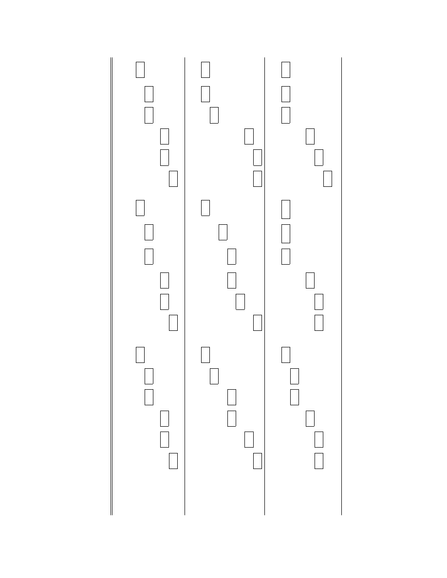
T

able

11:

Exp

ected

Utilit

y

b

y

T

rader

V

aluation

BHO

ERR

WEM

Priv

ate

value

Priv

ate

value

Priv

ate

value

P

ercen

t

-5.00

-2.50

-1.25

1.25

2.50

5.00

-5.00

-2.50

-1.25

1.25

2.50

5.00

-5.00

-2.50

-1.25

1.25

2.50

5.00

Cen

ts

-4.25

-2.12

-1.06

1.06

2.12

4.25

-9.68

-4.84

-2.42

2.44

4.84

9.68

-6.75

-3.38

-1.69

1.69

3.38

6.75

Lo

w

liquidit

y

state:

wide

spread,

lo

w

depth

Buy

mark

et

-6.31

-4.19

-3.13

-1.00

0.06

2.18

-13.65

-8.81

-6.39

-1.55

0.87

5.71

-9.94

-6.57

-4.88

-1.51

0.18

3.55

Buy

1

tic

k

-4.33

-2.45

-1.51

0.38

1.32

3.20

-8.99

-5.08

-3.13

0.77

2.73

6.63

-7.12

-4.26

-2.84

0.02

1.45

4.31

Buy

marginal

1.31

1.54

1.65

1.88

2.00

2.22

3.46

3.93

4.16

4.63

4.86

5.33

0.97

1.27

1.42

1.72

1.87

2.17

No

order

1.79

1.79

1.79

1.79

1.79

1.79

4.61

4.61

4.61

4.61

4.61

4.61

1.54

1.54

1.54

1.54

1.54

1.54

Sell

marginal

2.47

2.04

1.83

1.40

1.18

0.75

5.72

5.02

4.66

3.96

3.61

2.90

2.67

2.11

1.83

1.28

1.00

0.44

Sell

1

tic

k

3.16

1.28

0.35

-1.52

-2.46

-4.33

6.17

2.05

0.00

-4.12

-6.17

-10.29

3.64

1.64

0.64

-1.36

-2.36

-4.36

Sell

mark

et

2.18

0.06

-1.00

-3.13

-4.19

-6.31

4.56

-0.28

-2.70

-7.54

-9.96

-14.80

3.56

0.18

-1.51

-4.88

-6.57

-9.95

High

liquidit

y

state:

narro

w

spread,

high

depth

Buy

marginal

-4.36

-2.24

-1.18

0.95

2.01

4.13

-11.70

-6.86

-4.44

0.40

2.82

7.66

-7.23

-3.86

-2.17

1.20

2.89

6.26

Buy

1

tic

k

-0.27

0.55

0.95

1.77

2.17

2.99

1.28

2.35

2.89

3.97

4.51

5.58

-0.91

0.11

0.62

1.64

2.15

3.17

Buy

marginal

1.38

1.54

1.61

1.77

1.84

2.00

3.37

3.84

4.07

4.54

4.78

5.25

1.11

1.28

1.37

1.55

1.64

1.81

No

order

1.79

1.79

1.79

1.79

1.79

1.79

4.61

4.61

4.61

4.61

4.61

4.61

1.54

1.54

1.54

1.54

1.54

1.54

Sell

marginal

2.12

1.88

1.76

1.51

1.39

1.15

5.40

4.80

4.50

3.91

3.61

3.02

2.28

1.85

1.63

1.20

0.99

0.55

Sell

1

tic

k

2.81

2.05

1.67

0.91

0.53

-0.23

5.23

4.48

4.10

3.35

2.97

2.22

3.94

2.48

1.75

0.29

-0.44

-1.90

Sell

mark

et

4.13

2.01

0.95

-1.18

-2.24

-4.36

8.81

3.97

1.55

-3.29

-5.71

-10.55

6.27

2.89

1.20

-2.17

-3.86

-7.23

Mo

ving

mark

et

state:

common

value

pro

xy

higher

than

the

mid-quote

Buy

mark

et

-3.69

-1.52

-0.44

1.73

2.81

4.98

-5.12

-0.08

2.44

7.48

10.00

15.04

-6.04

-2.60

-0.87

2.57

4.29

7.73

Buy

1

tic

k

-0.77

0.44

1.04

2.25

2.86

4.07

3.72

4.12

4.32

4.72

4.92

5.32

-0.77

0.38

0.96

2.11

2.68

3.83

Buy

marginal

1.50

1.63

1.70

1.83

1.90

2.03

4.24

4.38

4.45

4.58

4.65

4.79

1.25

1.40

1.47

1.62

1.70

1.84

No

order

1.79

1.79

1.79

1.79

1.79

1.79

4.61

4.61

4.61

4.61

4.61

4.61

1.54

1.54

1.54

1.54

1.54

1.54

Sell

marginal

2.50

1.97

1.71

1.18

0.92

0.40

6.22

4.65

3.87

2.30

1.52

-0.05

2.53

1.85

1.51

0.83

0.49

-0.19

Sell

1

tic

k

2.35

0.77

-0.03

-1.61

-2.40

-3.99

2.48

-1.08

-2.86

-6.42

-8.20

-11.75

2.84

0.99

0.06

-1.78

-2.71

-4.56

Sell

mark

et

1.51

-0.66

-1.74

-3.91

-4.99

-7.16

-0.87

-5.91

-8.43

-13.47

-15.99

-21.03

2.36

-1.08

-2.81

-6.25

-7.97

-11.41

The

table

rep

orts

the

exp

ected

utilit

y

from

differen

t

order

submissions

for

traders

with

differen

t

priv

ate

values.

The

exp

ected

utilities

are

computed

for

three

differen

t

states;

a

lo

w

liquidit

y

state

where

the

bid-ask

spread

is

one

standard

deviation

ab

ov

e

its

mean

and

the

depth

variables

are

one

standard

deviation

b

elo

w

their

means,

a

high

liquidit

y

state

where

the

bid-ask

spread

is

one

standard

deviation

b

elo

w

its

mean

and

the

depth

variables

are

one

standard

deviation

ab

ov

e

their

mean

values,

and

a

mo

ving

mark

ets

state

where

the

common

value

pro

xy

divided

b

y

the

mid-quote

is

one

standard

deviation

ab

ov

e

its

mean.

All

other

variables

are

at

the

in-sample

mean

values.

All

utilities

are

rep

orted

in

cen

ts

p

er

share.

43

Table 12: Order Submission Probabilities by Trader Valuation

Private value

(−∞, −5%]

(−5%, −2.5%]

(−2.5%, +2.5%)

[2.5%, +5%)

[+5%, +∞)

BHO

Probability of value in interval

Mean

0.212

0.127

0.322

0.127

0.212

Standard deviation

0.026

0.007

0.039

0.007

0.026

Mean order submission probabilities

Sell market

0.735

0.247

0.014

0.000

0.000

Sell limit

0.244

0.642

0.247

0.003

0.000

No order

0.019

0.089

0.364

0.068

0.010

Buy limit

0.002

0.022

0.367

0.743

0.301

Buy market

0.000

0.000

0.008

0.187

0.689

Standard deviation of order submission probabilities

Sell market

0.300

0.357

0.070

0.010

0.000

Sell limit

0.286

0.393

0.201

0.042

0.006

No order

0.093

0.251

0.282

0.218

0.065

Buy limit

0.029

0.128

0.271

0.356

0.305

Buy market

0.000

0.004

0.050

0.316

0.309

ERR

Probability of value in interval

Mean

0.115

0.143

0.484

0.143

0.115

Standard deviation

0.018

0.009

0.049

0.009

0.018

Mean order submission probabilities

Sell market

0.851

0.316

0.011

0.001

0.000

Sell limit

0.147

0.656

0.164

0.001

0.000

No order

0.002

0.027

0.608

0.009

0.001

Buy limit

0.000

0.001

0.210

0.752

0.218

Buy market

0.000

0.000

0.007

0.238

0.781

Standard deviation of order submission probabilities

Sell market

0.233

0.351

0.059

0.026

0.008

Sell limit

0.231

0.355

0.116

0.030

0.011

No order

0.027

0.120

0.154

0.069

0.015

Buy limit

0.003

0.023

0.116

0.334

0.263

Buy market

0.000

0.000

0.039

0.330

0.264

WEM

Probability of value in interval

Mean

0.111

0.130

0.519

0.130

0.111

Standard deviation

0.017

0.012

0.055

0.012

0.017

Mean order submission probabilities

Sell market

0.921

0.483

0.036

0.000

0.000

Sell limit

0.079

0.512

0.413

0.003

0.000

No order

0.000

0.004

0.118

0.011

0.001

Buy limit

0.000

0.001

0.403

0.616

0.164

Buy market

0.000

0.000

0.030

0.370

0.835

Standard deviation of order submission probabilities

Sell market

0.157

0.413

0.090

0.001

0.000

Sell limit

0.157

0.411

0.171

0.047

0.008

No order

0.007

0.053

0.176

0.090

0.021

Buy limit

0.003

0.021

0.155

0.415

0.237

Buy market

0.002

0.007

0.089

0.414

0.238

The table reports the in-sample mean and the standard deviation of the probability of drawing a private value (u)
from five different intervals. For each interval and stock the table reports the in-sample mean and standard deviation
of the probability of a trader optimally submitting a sell market order, a sell limit order, no order, a buy limit order,
or a buy market order.

44

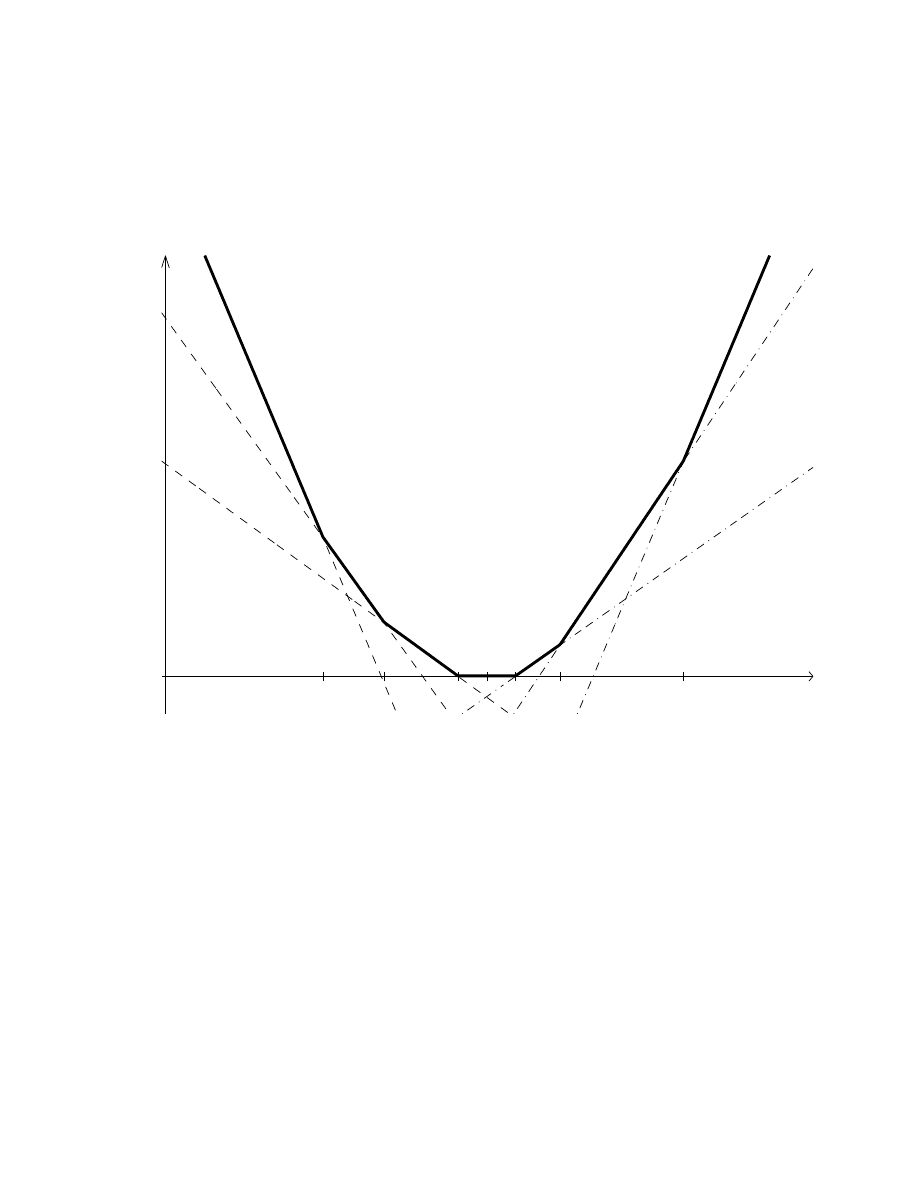
θ

sell

t

(0,1)

θ

sell

t

(1,2)

θ

sell

t

(2,NO)

θ

t

(2,2)

θ

buy

t

(2,NO)

θ

buy

t

(1,2)

θ

buy

t

(0,1)

Valuation v

t

=y

t

+u

0

Expected

Utility

←

E

t

[U

t,t+T

| d

buy

t,0

=1,u

t

]

←

E

t

[U

t,t+T

| d

buy

t,1

=1,u

t

]

←

E

t

[U

t,t+T

| d

buy

t,2

=1,u

t

]

E

t

[U

t,t+T

| d

sell

t,0

=1,u

t

]

→

E

t

[U

t,t+T

| d

sell

t,1

=1,u

t

]

→

E

t

[U

t,t+T

| d

sell

t,2

=1,u

t

]

→

Figure 1: The graph provides an example of the traders optimal order submission strategy. The
horizontal axis is the trader’s valuation, and the vertical axis is the expected utility from various
order submissions. The horizontal axis and the vertial axis have different scale. Sell orders are
plotted with dashed lines (- - -) and buy orders are plotted with dashed-dotted lines (-.-.). The
maximized utility function is plotted with a dark solid line (—). The continuation value is equal
to zero.

45

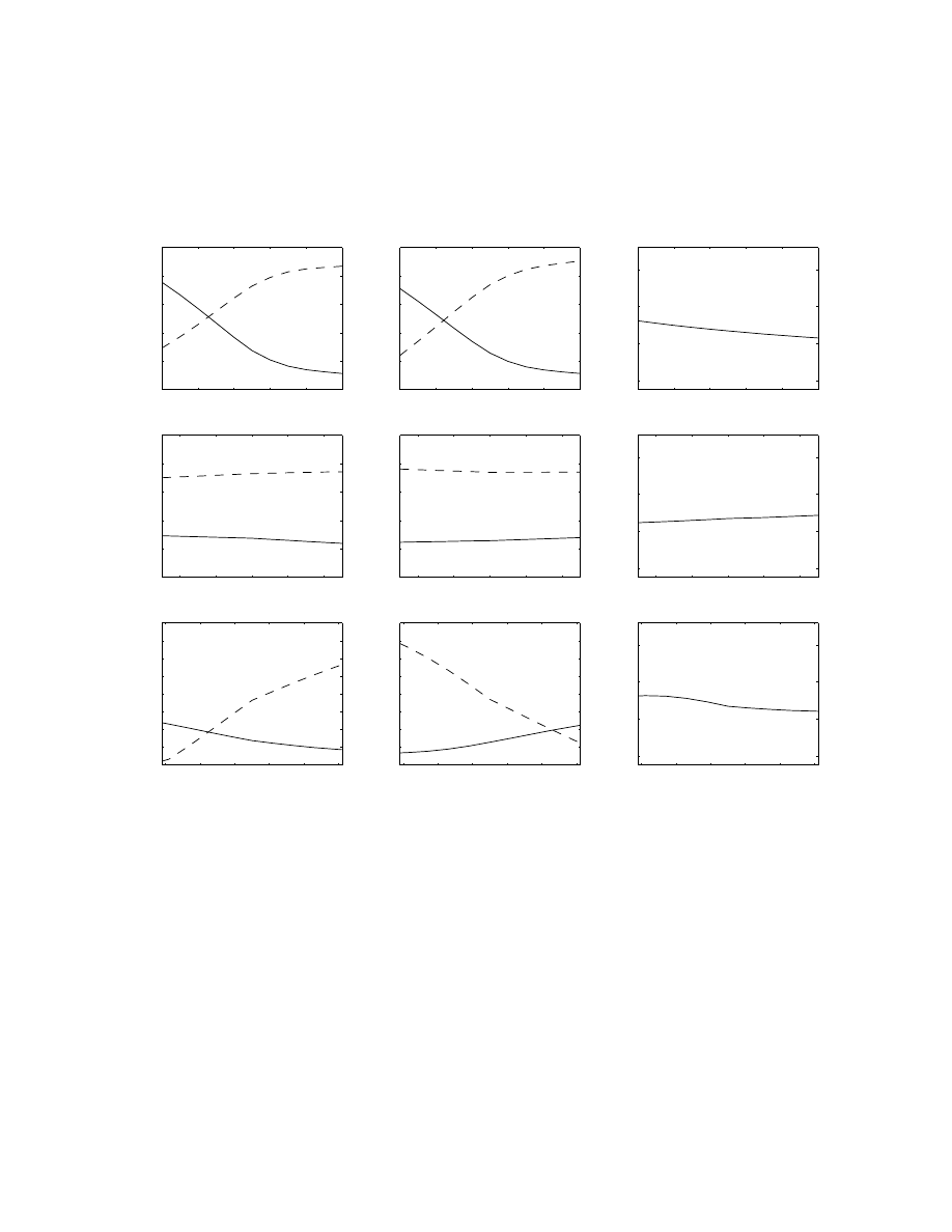
1

2

3

4

5

6

0

0.1

0.2

0.3

0.4

0.5

Spread [%]

Sell Choice Prob.

1

2

3

4

5

6

0

0.1

0.2

0.3

0.4

0.5

Spread [%]

Buy Choice Prob.

1

2

3

4

5

6

150

200

250

300

Spread [%]

Time to next order

0.5

0.75

1.0

2.5

4.0

0

0.1

0.2

0.3

0.4

0.5

Bid Depth

Sell Choice Prob.

0.5

0.75

1.0

2.5

4.0

0

0.1

0.2

0.3

0.4

0.5

Bid Depth

Buy Choice Prob.

0.5

0.75

1.0

2.5

4.0

150

200

250

300

Bid Depth

Time to next order

−2.5

−1.5

−0.5

0.5

1.5

2.5

0

0.1

0.2

0.3

0.4

0.5

0.6

0.7

0.8

Common Value − Mid−Quote [%]

Sell Choice Prob.

−2.5

−1.5

−0.5

0.5

1.5

2.5

0

0.1

0.2

0.3

0.4

0.5

0.6

0.7

0.8

Common Value − Mid−Quote [%]

Buy Choice Prob.

−2.5

−1.5

−0.5

0.5

1.5

2.5

150

200

250

300

Common Value − Mid−Quote [%]

Time to next order

Figure 2: Comparative statics for BHO. The top left picture plots the probability of a sell market
order (–) and the probability of a sell limit order (- -) conditional on an order submission as a
function of the spread. The top middle picture plots the probability of a buy market order (–) and
the probability of a buy limit order (- -) conditional on an order submission as a function of the
spread. The top right picture plots the expected time to the next order submission as a function of
the spread. The middle row and the bottom row of pictures plots the corresponding comparative
statics for the choice probabilities and time to the next order for the bid side depth and the distance
between the common value proxy and the mid-quote.

46

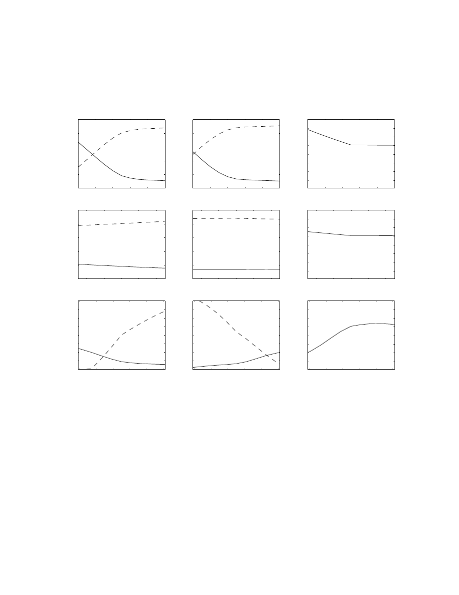
1

2

3

4

5

6

0

0.1

0.2

0.3

0.4

0.5

Spread [%]

Sell Choice Prob.

1

2

3

4

5

6

0

0.1

0.2

0.3

0.4

0.5

Spread [%]

Buy Choice Prob.

1

2

3

4

5

6

140

160

180

200

220

240

260

280

Spread [%]

Time to next order

0.5

0.75

1.0

2.5

4.0

0

0.1

0.2

0.3

0.4

0.5

Bid Depth

Sell Choice Prob.

0.5

0.75

1.0

2.5

4.0

0

0.1

0.2

0.3

0.4

0.5

Bid Depth

Buy Choice Prob.

0.5

0.75

1.0

2.5

4.0

140

160

180

200

220

240

260

280

Bid Depth

Time to next order

−2.5

−1.5

−0.5

0.5

1.5

2.5

0

0.1

0.2

0.3

0.4

0.5

0.6

0.7

0.8

Common Value − Mid−Quote [%]

Sell Choice Prob.

−2.5

−1.5

−0.5

0.5

1.5

2.5

0

0.1

0.2

0.3

0.4

0.5

0.6

0.7

0.8

Common Value − Mid−Quote [%]

Buy Choice Prob.

−2.5

−1.5

−0.5

0.5

1.5

2.5

140

160

180

200

220

240

260

280

Common Value − Mid−Quote [%]

Time to next order

Figure 3: Comparative statics for ERR. The top left picture plots the probability of a sell market
order (–) and the probability of a sell limit order (- -) conditional on an order submission as a
function of the spread. The top middle picture plots the probability of a buy market order (–) and
the probability of a buy limit order (- -) conditional on an order submission as a function of the
spread. The top right picture plots the expected time to the next order submission as a function of
the spread. The middle row and the bottom row of pictures plots the corresponding comparative
statics for the choice probabilities and time to the next order for the bid side depth and the distance
between the common value proxy and the mid-quote.

47

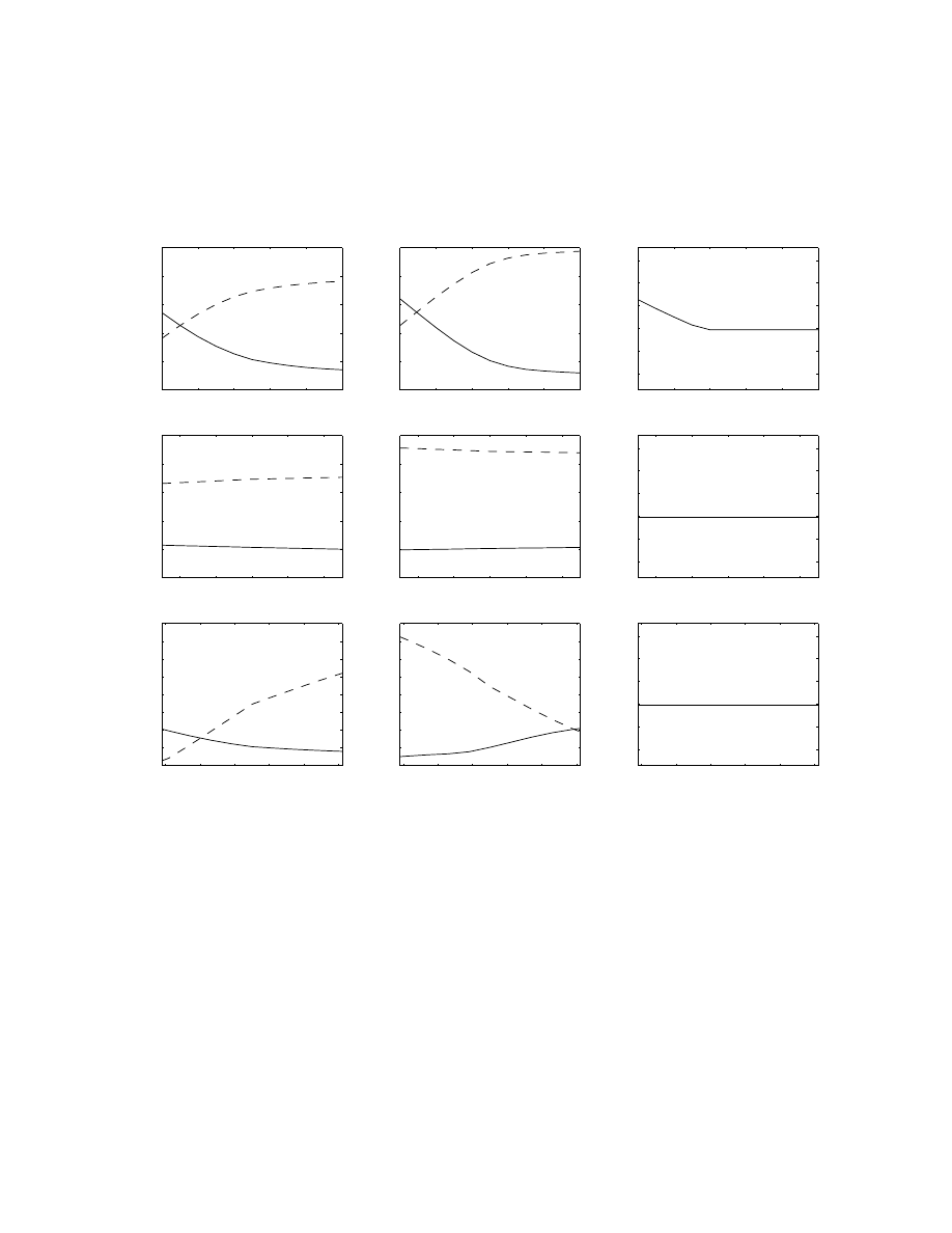
1

2

3

4

5

6

0

0.1

0.2

0.3

0.4

0.5

Spread [%]

Sell Choice Prob.

1

2

3

4

5

6

0

0.1

0.2

0.3

0.4

0.5

Spread [%]

Buy Choice Prob.

1

2

3

4

5

6

300

350

400

450

500

550

Spread [%]

Time to next order

0.5

0.75

1.0

2.5

4.0

0

0.1

0.2

0.3

0.4

0.5

Bid Depth

Sell Choice Prob.

0.5

0.75

1.0

2.5

4.0

0

0.1

0.2

0.3

0.4

0.5

Bid Depth

Buy Choice Prob.

0.5

0.75

1.0

2.5

4.0

300

350

400

450

500

550

Bid Depth

Time to next order

−2.5

−1.5

−0.5

0.5

1.5

2.5

0

0.1

0.2

0.3

0.4

0.5

0.6

0.7

0.8

Common Value − Mid−Quote [%]

Sell Choice Prob.

−2.5

−1.5

−0.5

0.5

1.5

2.5

0

0.1

0.2

0.3

0.4

0.5

0.6

0.7

0.8

Common Value − Mid−Quote [%]

Buy Choice Prob.

−2.5

−1.5

−0.5

0.5

1.5

2.5

300

350

400

450

500

550

Common Value − Mid−Quote [%]

Time to next order

Figure 4: Comparative statics for WEM. The top left picture plots the probability of a sell market
order (–) and the probability of a sell limit order (- -) conditional on an order submission as a
function of the spread. The top middle picture plots the probability of a buy market order (–) and
the probability of a buy limit order (- -) conditional on an order submission as a function of the
spread. The top right picture plots the expected time to the next order submission as a function of
the spread. The middle row and the bottom row of pictures plots the corresponding comparative
statics for the choice probabilities and time to the next order for the bid side depth and the distance
between the common value proxy and the mid-quote.

48

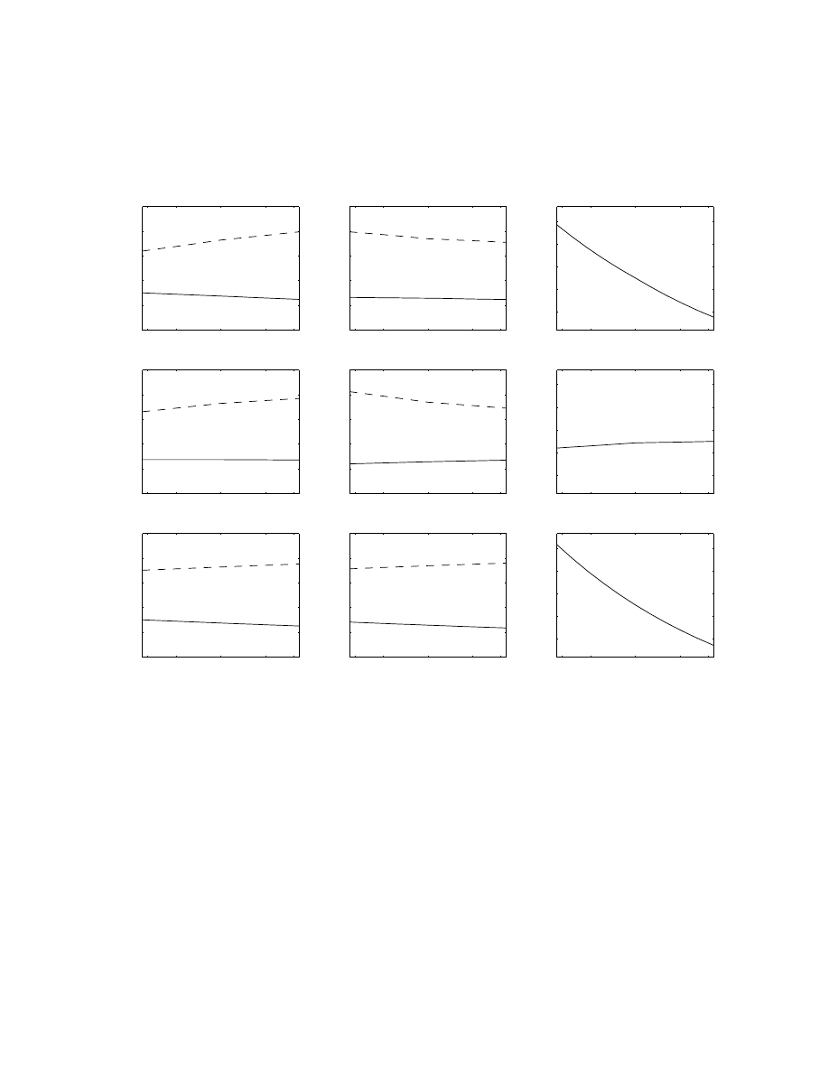
0.1

0.35

0.75

1.15

1.4

0

0.1

0.2

0.3

0.4

0.5

Lagged Return

Sell Choice Prob.

0.1

0.35

0.75

1.15

1.4

0

0.1

0.2

0.3

0.4

0.5

Lagged Return

Buy Choice Prob.

0.1

0.35

0.75

1.15

1.4

0

0.1

0.2

0.3

0.4

0.5

Lagged Return

Sell Choice Prob.

0.1

0.35

0.75

1.15

1.4

0

0.1

0.2

0.3

0.4

0.5

Lagged Return

Buy Choice Prob.

0.1

0.35

0.75

1.15

1.4

0

0.1

0.2

0.3

0.4

0.5

Lagged Return

Sell Choice Prob.

0.1

0.35

0.75

1.15

1.4

0

0.1

0.2

0.3

0.4

0.5

Lagged Return

Buy Choice Prob.

0.1

0.35

0.75

1.15

1.4

80

100

120

140

160

Lagged Return

Time to next order

0.1

0.35

0.75

1.15

1.4

80

100

120

140

160

Lagged Return

Time to next order

0.1

0.35

0.75

1.15

1.4

80

100

120

140

160

Lagged Return

Time to next order

Figure 5: Comparative statics for BHO. The top left picture plots the sell market (–) and sell
limit (- -) choice probabilities as a function of the absolute value of changes in the stock’s lagged
return. The top middle picture plots the buy market (–) and buy limit (- -) choice probabilities as
a function of the absolute value of changes in the stock’s lagged return. The top right picture plots
the expected time to the next order submission as a function of the absolute value of changes in the
stock’s lagged return. The middle and the bottom row of pictures also plot the choice probabilities
and time to the next order submission. In the middle row of pictures the valuation distribution
and the arrival rate of traders are held constant at their mean values and in the bottom row of
pictures the threshold valuations are held constant at their mean values.

49

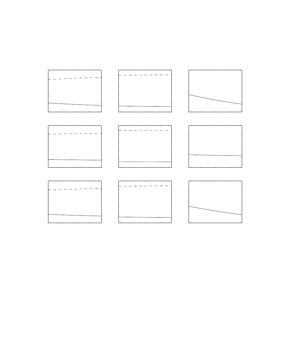
0.1

0.35

0.75

1.15

1.4

0

0.1

0.2

0.3

0.4

0.5

Lagged Return

Sell Choice Prob.

0.1

0.35

0.75

1.15

1.4

0

0.1

0.2

0.3

0.4

0.5

Lagged Return

Buy Choice Prob.

0.1

0.35

0.75

1.15

1.4

0

0.1

0.2

0.3

0.4

0.5

Lagged Return

Sell Choice Prob.

0.1

0.35

0.75

1.15

1.4

0

0.1

0.2

0.3

0.4

0.5

Lagged Return

Buy Choice Prob.

0.1

0.35

0.75

1.15

1.4

0

0.1

0.2

0.3

0.4

0.5

Lagged Return

Sell Choice Prob.

0.1

0.35

0.75

1.15

1.4

0

0.1

0.2

0.3

0.4

0.5

Lagged Return

Buy Choice Prob.

0.1

0.35

0.75

1.15

1.4

100

150

200

Lagged Return

Time to next order

0.1

0.35

0.75

1.15

1.4

100

150

200

Lagged Return

Time to next order

0.1

0.35

0.75

1.15

1.4

100

150

200

Lagged Return

Time to next order

Figure 6: Comparative statics for ERR. The top left picture plots the sell market (–) and sell
limit (- -) choice probabilities as a function of the absolute value of changes in the stock’s lagged
return. The top middle picture plots the buy market (–) and buy limit (- -) choice probabilities as
a function of the absolute value of changes in the stock’s lagged return. The top right picture plots
the expected time to the next order submission as a function of the absolute value of changes in the
stock’s lagged return. The middle and the bottom row of pictures also plot the choice probabilities
and time to the next order submission. In the middle row of pictures the valuation distribution
and the arrival rate of traders are held constant at their mean values and in the bottom row of
pictures the threshold valuations are held constant at their mean values.

50

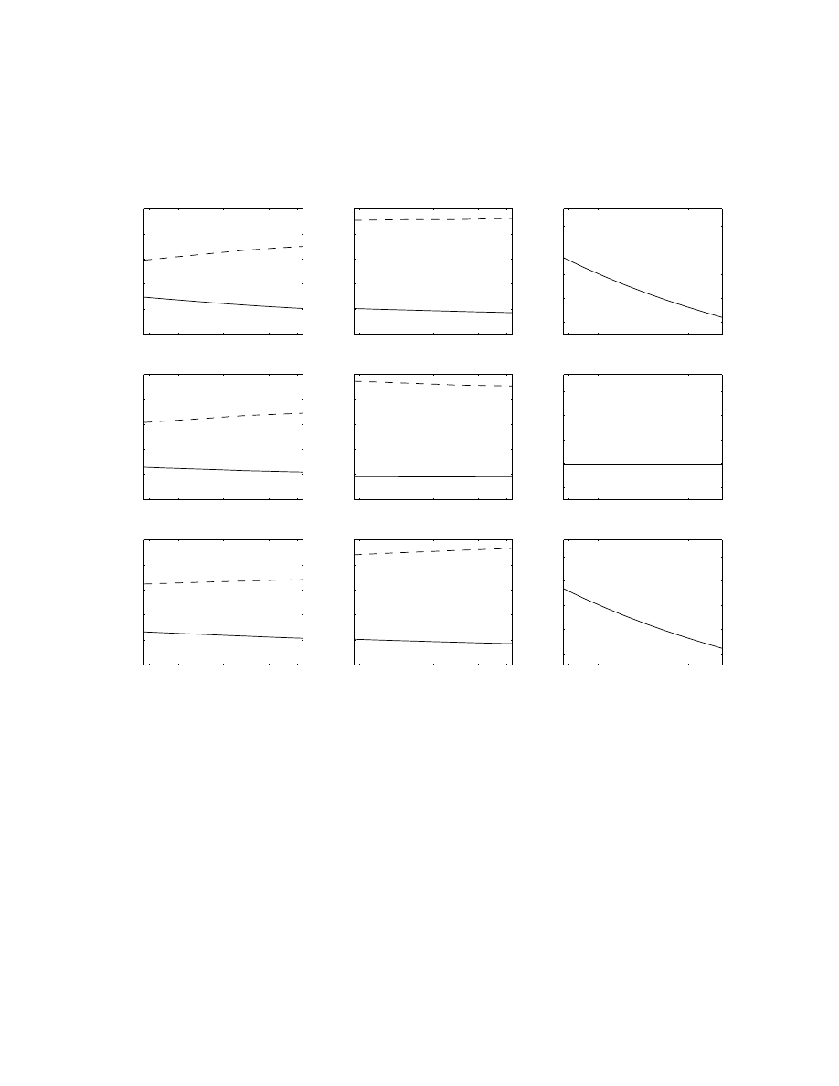
0.1

0.35

0.75

1.15

1.4

0

0.1

0.2

0.3

0.4

0.5

Lagged Return

Sell Choice Prob.

0.1

0.35

0.75

1.15

1.4

0

0.1

0.2

0.3

0.4

0.5

Lagged Return

Buy Choice Prob.

0.1

0.35

0.75

1.15

1.4

0

0.1

0.2

0.3

0.4

0.5

Lagged Return

Sell Choice Prob.

0.1

0.35

0.75

1.15

1.4

0

0.1

0.2

0.3

0.4

0.5

Lagged Return

Buy Choice Prob.

0.1

0.35

0.75

1.15

1.4

0

0.1

0.2

0.3

0.4

0.5

Lagged Return

Sell Choice Prob.

0.1

0.35

0.75

1.15

1.4

0

0.1

0.2

0.3

0.4

0.5

Lagged Return

Buy Choice Prob.

0.1

0.35

0.75

1.15

1.4

150

200

250

300

350

Lagged Return

Time to next order

0.1

0.35

0.75

1.15

1.4

150

200

250

300

350

Lagged Return

Time to next order

0.1

0.35

0.75

1.15

1.4

150

200

250

300

350

Lagged Return

Time to next order

Figure 7: Comparative statics for WEM. The top left picture plots the sell market (–) and sell
limit (- -) choice probabilities as a function of the absolute value of changes in the stock’s lagged
return. The top middle picture plots the buy market (–) and buy limit (- -) choice probabilities as
a function of the absolute value of changes in the stock’s lagged return. The top right picture plots
the expected time to the next order submission as a function of the absolute value of changes in the
stock’s lagged return. The middle and the bottom row of pictures also plot the choice probabilities
and time to the next order submission. In the middle row of pictures the valuation distribution
and the arrival rate of traders are held constant at their mean values and in the bottom row of
pictures the threshold valuations are held constant at their mean values.

51