Anatomy of a Cortical Simulator

Rajagopal Ananthanarayanan

IBM Almaden Research Center

650 Harry Road

San Jose, CA

[e-mail]

Dharmendra S. Modha

IBM Almaden Research Center

650 Harry Road

San Jose, CA

[e-mail]

ABSTRACT

Insights into brain’s high-level computational principles will
lead to novel cognitive systems, computing architectures,
programming paradigms, and numerous practical applica-
tions. An important step towards this end is the study of
large networks of cortical spiking neurons.

We have built a cortical simulator, C2, incorporating several
algorithmic enhancements to optimize the simulation scale
and time, through: computationally efficient simulation of
neurons in a clock-driven and synapses in an event-driven
fashion; memory efficient representation of simulation state;
and communication efficient message exchanges.

Using phenomenological, single-compartment models of spik-
ing neurons and synapses with spike-timing dependent plas-
ticity, we represented a rat-scale cortical model (55 million
neurons, 442 billion synapses) in 8TB memory of a 32,768-
processor BlueGene/L. With 1 millisecond resolution for
neuronal dynamics and 1-20 milliseconds axonal delays, C2
can simulate 1 second of model time in 9 seconds per Hertz
of average neuronal firing rate.

In summary, by combining state-of-the-art hardware with
innovative algorithms and software design, we simultane-
ously achieved unprecedented time-to-solution on an un-
precedented problem size.

1.

INTRODUCTION

The cerebral cortex is believed to be the seat of cognition.
Unraveling the computational and operational function of
the cortex is a grand challenge with enormous implications
for cognitive computing. Large-scale cortical simulations
provide one avenue for computationally exploring hypothe-
ses about how does the cortex work, what does it compute,
and how we may, eventually, mechanize it.

A simple view of the cortex is that it consists of discrete
units: neurons. Each neuron receives inputs from thousands

Permission to make digital or hard copies of all or part of this work for
personal or classroom use is granted without fee provided that copies are
not made or distributed for profit or commercial advantage, and that copies
bear this notice and the full citation on the first page. To copy otherwise, to
republish, to post on servers or to redistribute to lists, requires prior specific
permission and/or a fee.

SC07 November 10-16, 2007, Reno, Nevada, USA (c) 2007 ACM 978-1-
59593-764-3/07/0011

. . .

$5.00

of neurons via its dendrites and, in turn, connects to thou-
sands of others via its axon. The point of contact between an
axon of a neuron and a dendrite on another neuron is called
a synapse; and, with respect to the synapse, the two neu-
rons are respectively called pre-synaptic and post-synaptic.
If some event such as an incoming stimulus causes the neu-
ron membrane potential to rise above a certain threshold,
the neuron will fire sending a spike down its axon. All the
synapses that the axon contacts are then activated after an
appropriate axonal conductance delay. Neurons can either
be excitatory meaning that their firing makes those neurons
whose synapses it contacts more likely to fire or inhibitory.
Finally, synapses made by excitatory neurons are plastic,
that is, the effect of their activation on the corresponding
post-synaptic neuron is subject to change over time using
a plasticity rule such as spike-timing dependent plasticity
(STDP) [26]. STDP rule potentiates (increases the weight
of) a synapse if its post-synaptic neuron fires after its pre-
synaptic neuron fires, and depresses (decreases the weight
of) a synapse if the order of two firings is reversed. For
an excellent theoretical treatment of computational neuro-
science, please see [6].

Cortical simulations have a rich history dating back to two
classic papers in 1954 [9] and 1956 [20]. A detailed review
of the entire field of cortical simulations is beyond the scope
of this paper; for a recent extensive review and comparison
of a number of publicly available cortical simulators (NEU-
RON, GENESIS, NEST, NCS, CSIM, XPPAUT, SPLIT,
and Mvaspike) using spiking neurons, please see [4]. For
event-driven simulators using spiking neurons, see [7, 17,
22, 30]. Design of a general purpose cortical simulator in
a distributed multiprocessor setting was described in [18].
Recently, [16] discussed a (slightly larger than) mouse-scale
simulation using 1.6 × 10

6

units and 200 × 10

9

connections

corresponding to an artificial neural network; however, their
simulation is not based on spiking neurons with synaptic
plasticity which is the main focus here.

To study emergent dynamics and information-processing ca-
pacity of large networks of spiking neurons, the network
scale is essential. Scale is also important to incorporate
distance-dependent axonal conductance delays. In trying to
understand the computational function of the cortex, several
hypotheses regarding network topologies, neuron/synapse
models, etc., need to be tried out quickly. In addition, to
achieve steady state, some simulation experiments may need
to run for a long time such as 24 hours of simulated time

[15]. Thus, simulation time is also of essence. The main
focus of this paper is to understand computational princi-
ples underlying cortical simulations with the view towards
scalable and fast simulations.

Specifically, we consider the following challenge. The to-
tal surface area of the two hemispheres of the rat cortex is
roughly 600 mm

2

[19]. The number of neurons under 1 mm

2

of the mouse cortex is roughly 9.2 × 10

4

[23] and remains

roughly the same in rat [21]. Therefore, the rat cortex has
55.2 × 10

6

neurons. Taking the number of synapses per neu-

ron to be 8, 000 [3], there are roughly 442 × 10

9

synapses in

the rat cortex. Simulations at this scale in near real-time
impose tremendous constraints on computation, communi-
cation, and memory capacity of any computing platform.
For example, assuming that neurons fire at an average rate
of 1 Hz, each neuron would communicate with each of its
synaptic targets once a second, resulting in an average total
of 442 billion messages per second. Roughly, 80% of the cor-
tical neurons are excitatory [3]. The state of the synapses
made by these excitatory neurons must be updated once
a second as per STDP. For near real-time performance for
these synaptic updates, all synapses must fit within the main
memory of the system. Finally, in a discrete-event simula-
tion setting, the state of all neurons must be updated every
simulation time step which could be 1 ms or smaller. At the
complexity of neurons and synapses that we have used, the
computation, communication, and memory requirements all
scale with the number of synapses which outnumber the
number of neurons by a factor of 8, 000.

To address these challenges, we have designed and imple-
mented a massively parallel cortical simulator, C2, designed
to run on distributed memory multiprocessors.

C2 is developed as part of the Cognitive Computing project
at IBM’s Almaden Research Center. The goal of our project
is to develop novel cognitive systems, computing architec-
tures, programming paradigms, and to explore their practi-
cal business/enterprise applications – by gaining an opera-
tional, computational understanding of how the brain works.
The project involves abstract, high-level, phenomenological
neuroscience models that are tractable on contemporary su-
percomputers. IBM is also a participant (along with many
others) in a large project called Blue Brain, that is cen-
tered at the Ecole Polytechnique Federale de Lausanne. The
Blue Brain project will be constructing and simulating very
detailed, biologically accurate models of the brain at the
molecular level, with a goal of obtaining deep biological un-
derstanding of how the brain works. Such detailed models
draw on the latest advances in the area of neuroscience and
will require orders of magnitude more computational capa-
bility than currently exists

1

.

The rest of the paper is organized as follows. In Section 2, we
outline our main contributions. In Section 3, we present the
overall design of C2 along with detailed algorithms. In Sec-
tions 4 and 5, we discuss the simulated models and results,
and present discussion and concluding remarks in Section 6.

1

We are grateful to Dr. Eric Kronstadt for this remark concerning

Blue Brain. For more information, please contact Professor Henry
Markram, EPFL.

2.

CONTRIBUTIONS

C2 incorporates several algorithmic enhancements: (a) a
computationally efficient way to simulate neurons in a clock-
driven (“synchronous”) and synapses in an event-driven (“asyn-
chronous”) fashion; (b) a memory efficient representation to
compactly represent the state of the simulation; (c) a com-
munication efficient way to minimize the number of messages
sent by aggregating them in several ways and by mapping
message exchanges between processors onto judiciously cho-
sen MPI primitives for synchronization.

2.1

Architecture

We briefly describe the general architecture of C2 which fol-
lows [18], but additionally incorporates STDP. By modeling
neuronal and synaptic dynamics using difference equations
and by discretizing the spike times and the axonal conduc-
tance delays to a grid, for example, 1 ms, cortical simulations
can be thought of in the framework of discrete-event simu-
lations. We update the state of each neuron at every time
step, that is, in a clock-driven or synchronous fashion but up-
date the state of each excitatory synapse in an event-driven
or asynchronous fashion when either the corresponding pre-
synaptic or post-synaptic neuron fires. To summarize, the
overall algorithm is as follows:

Neuron

: For every neuron and for every simulation time

step (say 1 ms), update the state of each neuron. If the neu-
ron fires, generate a message (an event) for each synapse for
which the neuron is pre-synaptic at an appropriate future
time corresponding to the axonal conductance delay associ-
ated with the synapse. Also, if the neuron fires, potentiate
the synapses for which the neuron is post-synaptic according
to STDP.

Synapse: For every synapse, when it receives a message from
its presynaptic neuron, depress the synapse according to
STDP, and update the state of its post-synaptic neuron.

2.2

Algorithm

Computation: To enable a true event-driven processing of
synapses, for every neuron, we maintain a list of synapses
that were activated since the last time the neuron fired. In-
tuitively, we cache the recently activated synapses. This
list is useful when potentiating synapses according to STDP
when a post-synaptic neuron fires. Typically, the size of
this list is far smaller than the total number of synapses at-
tached to the neurons. Also, for each neuron we maintain
an ordered list of equivalence classes of synapses made by
the neuron that have the same delay along its axon. Once a
neuron fires, we only need to store the class of synapses that
will be activated in the nearest future in an event queue,
and, proceeding recursively, when that class of synapses is
activated, we insert the next class of synapses at an appro-
priate future time in the event queue. This recursion is use-
ful when depressing synapses according to STDP. Assuming
an average neuronal firing rate of 1 Hz and time steps of 1
ms, event-driven processing touches each synapse only once
a second while clock-driven processing would touch every
synapse at every millisecond – a factor 1,000.

Memory: Since synapses outnumber neurons by a factor of
8, 000, the scale of models is essentially limited by the num-
ber of synapses that will fit in available memory and by the

required transient memory. The above recursive structure
for storing events reduces the transient memory necessary
for buffering spikes. Additionally, we used minimal storage
for each synapse consisting of the synaptic weight, the time
step at which the synapses was activated (for STDP cal-
culation), the pointer to the next synapse of the activated
synapse list, one bit indicating whether a synapse is on the
list of activated synapses, and a pointer to the post-synaptic
neuron – a total of only 16 bytes per synapse.

Communication: A simple algorithm for communicating be-
tween neurons would generate a message for every synapse
that a neuron sends its axon to. In our algorithm, all den-
drites of a neuron always reside with it on the same proces-
sor, but its axon may be distributed [17]. With this assump-
tion, all synapses made by an axon on a distant processor
can be activated with a single message thus reducing the
number of messages from the order of synapses to the order
of average number of processors that a neuron connects to.
Furthermore, multiple axons originating from a processor
may travel to the same destination processor enabling fur-
ther message aggregation (and thus reduction in the num-
ber of messages) depending upon the average neuronal firing
rate.

We now turn to optimizations in the choice of communi-
cation primitives. Let us suppose that there are N dis-
tributed processors over which the neurons are distributed.
The destination processor D of a message does not know
that a particular source processor S is sending it a message
– and, hence, the two processors must synchronize. Recently
proposed algorithm in [18] uses a blocking communication
scheme where Send(D) on S requires Receive(S) on D and
both machines wait until these calls have finished. In their
scheme, to prevent deadlock, in a synchronization phase
preceding the communication phase, the Complete Pairwise
EXchange (CPEX) algorithm is employed. CPEX algorithm
requires roughly N communication steps each of which has
every processor either sending or receiving a message. In
contrast, we use a scheme where each source processor sim-
ply transmits the message in a non-blocking fashion. Then,
we use a synchronization scheme that requires only 2 com-
munication steps independent of the number of the proces-
sors to synchronize. In the first Reduce step each processor
sends to a predestined processor, say, processor 0, a message
saying how many messages it intends to send to every other
processor and in the second Scatter step processor 0 sends to
each processor the combined total number of messages that
it should receive from all the other processors. Equipped
with this knowledge, each processor can now retrieve the
messages destined for it in a blocking fashion. By design,
there is no possibility of deadlock in our scheme.

Our choice of communication primitives is designed to lever-
age knowledge of the application at hand. These primitives
themselves have been well understood and are highly op-
timized from an algorithmic perspective, for example, re-
cursive halving for commutative Reduce-Scatter [27]. We
used Reduce-Scatter for a commutative summation opera-
tion, and, hence, automatically benefit from these algorith-
mic advances.

The algorithm in [27] resorts to pairwise

exchange algorithm in the worst case, which implies that
the algorithm in [18] does not fully exploit the applica-

tion knowledge. Further, the implementation of the prim-
itives can take advantage of platform-specific features, for
example, BlueGene/L specific optimizations are detailed in
[1]. For the n-dimensional torus topology of BlueGene/L
(n = 3), Reduce-Scatter can be achieved in log

2

n+1

(number

of processors) steps [5].

2.3

Simulation Results

We deployed C2 on a 32, 768-processor BlueGene/L super-
computer [11]. Each processor operates at a clock frequency
of 700 MHz and has 256 MB of local main memory. Us-
ing phenomenological, single-compartment models of spik-
ing neurons [14, 15] and synapses with spike-timing depen-
dent plasticity [26], we were able to a represent nearly 57.76
million neurons and 461 billion synapses – at rat-scale – in
the main memory. We used a cortical network with: (a)
80% excitatory neurons and 20% inhibitory neurons [3]; (b)
a 0.09 local probability of connections [3]; and (c) axonal
conduction delays between 1-20 millisecond (ms) for exci-
tatory and 1 ms for inhibitory neurons. The neurons are
interconnected in a certain probabilistic fashion which is de-
scribed in detail later in this paper. For a network operating
at 7.2 Hz average neuronal firing rate in a stable, rhythmic
pattern, we were able to simulate 5 second (s) of model time
in 325 s while using a 1 millisecond resolution for neuronal
dynamics and axonal conductance delays. The simulation
time increases with the average firing rate, hence, it is use-
ful to specify a normalized value of the simulation run-time
[13, p. 1680]. When normalized to 1 Hz average firing rate,
this amounts to 1 s of model time in approximately 9 s (=
325/(7.2 × 5)) of real-time.

3.

THE DESIGN OF THE SIMULATOR C2

To motivate the design of our simulator in a distributed
multiprocessor setting, we first begin with the description of
optimized underlying logic in a single processor setting.

3.1

Single Processor Algorithm

Let us assume that all spikes are discretized to a grid with
1 ms resolution. Let the axonal delay of every neuron be an
integer in the range [1, δ], where δ is the event horizon.

For neuron n, let S(n, d) denote the set of synapses to which
its axon connects with delay d. For some delay d, the set
S(n, d) can be empty. Let D(n) denote the smallest delay
such that the corresponding set of synapses S(n, D(n)) is
non-empty.

Let E(i), 1 ≤ i ≤ δ, denote the set of synapses to be acti-
vated in future. These event sets are organized in a circular
queue of length δ such that the set of events E(mod(t, δ)+1)
will be processed at time t. All sets E(i), 1 ≤ i ≤ δ, are
initialized to be empty.

The complete algorithm for the single processor case is de-
scribed in Figure 1. The algorithm is described for a single
time step.

The steps SynAct1, SynAct2, DSTDP, and PSTDP
deal with synaptic computation, while the step NrnUpd
deals with neuronal computation. Step B2 is just a book-
keeping step. The steps SynAct1, SynAct2, DSTDP,

B1

x = MPI Comm rank(),N = MPI Comm size().

SynAct1

(Process current events) Activate synapses in

the set E(mod(t, δ) + 1).

SynAct2

(Generate future events) For each set S(n, d) in

E(mod(t, δ) + 1), if there exists a delay d

′

such that

d < d

′

≤ δ and S(n, d

′

) is non-empty, then insert

S(n, d

′

) in the set E(mod(t + d

′

− d, δ) + 1). Finally,

clear the set E(mod(t, δ) + 1).

DSTDP

For each synapse that is activated,

1. Update the state of the post-synaptic neuron n

by the associated synaptic weight.

2. If the synapse if excitatory, depress the synapse

according to STDP and put the synapse on the
list of recently activated synapses R(n) for the
corresponding neuron n.

B2

Set the list F of fired neurons to be empty set.

M

x

(y) =

0, 1 ≤ y ≤ N .

NrnUpd

For each neuron n, with some stimulus probabil-

ity, provide it with a super-threshold stimulus, update
its state, and if it fires, then (a) reset the neuron state,
(b) add the neuron to list F , and (c)

N1

insert set S(n, D(n)) into the event set E(mod(t+

D(n), δ) + 1).

FlsgMsg

Flush any non-empty, non-full messages destined

for any processor y using MPI Isend. Increment the
number of messages sent M

x

(y) by 1.

PSTDP

For every neuron n in list F , and for each of its

synapse on the list R(n), reward the synapse accord-
ing to STDP. Clear the list R(n).

MeX1

Using MPI ReduceScatter send M

x

(1), . . . , M

x

(N )

to processor 0 and receive the count of incoming mes-
sages to this processor M (x) =

P

N
y=1

M

y

(x).

MeX2

Using MPI Recv, receive M (x) messages each of the

form (m, z). Now, for each message,

N1

insert S((m, z), D(m, z; x); x) into the event set

E

x

(mod(t + D(m, z; x), δ) + 1).

Figure 1: Single processor algorithm at time step t.

B1

x = MPI Comm rank(), N = MPI Comm size().

SynAct1

(Process current events) Activate synapses in

the set E

x

(mod(t, δ) + 1).

SynAct2

(Generate

future

events)

For

each

set

S((m, z), d; x) in E

x

(mod(t, δ) + 1), if there exists

a delay d

′

such that d < d

′

≤ δ and S((m, z), d

′

; x)

is non-empty, then insert S((m, z), d

′

; x) in the set

E

x

(mod(t + d

′

− d, δ) + 1).

Finally, clear the set

E

x

(mod(t, δ) + 1).

DSTDP

For each synapse that is activated,

1. Update the state of the post-synaptic neuron n

by the associated synaptic weight.

2. If the synapse if excitatory, depress the synapse

according to STDP and put the synapse on the
list of recently activated synapses R(n) for the
corresponding neuron n.

B2

Set the list F of fired neurons to be empty set. Initialize

M

x

(y) = 0, 1 ≤ y ≤ N .

NrnUpd

For each neuron n, with some stimulus probabil-

ity, provide it with a super-threshold stimulus, update
its state, and if it fires, then (a) reset the neuron state,
(b) add the neuron to list F , and (c) if the neuron con-
nects to any synapse on processor y, then prepare to
send a message (n, x) to processor y by adding n to
a message destined from x to y. If the message be-
comes full, then send it using MPI Isend. Increment
the number of messages sent M

x

(y).

FlshMsg

Flush any non-empty, non-full messages destined

for any processor y using MPI Isend. Increment the
number of messages sent M

x

(y) by 1.

PSTDP

For every neuron n in list F , and for each of its

synapse on the list R(n), reward the synapse accord-
ing to STDP. Clear the list R(n).

MeX1

Using MPI ReduceScatter send M

x

(1), . . . , M

x

(N )

to processor 0 and receive the count of incoming mes-
sages to this processor M (x) =

P

N
y=1

M

y

(x).

MeX2

Using MPI Recv, receive M (x) messages each of the

form (m, z). Now, for each message,

N1

insert set S((m, z), D(m, z; x); x) into the event

set E

x

(mod(t + D(m, z; x), δ) + 1).

Figure 2: Distributed algorithm at time step t on processor
x.

and PSTDP are event-driven, and are asynchronous in na-
ture, whereas step NrnUpd is clock-driven and is synchronous.
This is an essential characteristic of the algorithm. While
every neuron is updated at every time step, the synapses
are processed only when either they are activated by an in-
coming message or their corresponding post-synaptic neu-
ron fires. Furthermore, for each neuron n, we maintain a
list R(n) of synapses that have been activated since the last
time the neuron fired. Typically, the size of list R(n) is sig-
nificantly smaller than the total number of synapses that
the neuron is post-synaptic to, and, hence, step PSTDP
can be executed with considerable speed. The step N1 is a
crucial link that connects the synchronous computation in
NrnUpd

to event-driven computation in SynAct1, Syn-

Act2

, and DSTDP. When extending the single processor

algorithm to distributed setting, we will introduce several
new steps to implement a similar link. Now, we explain
each step.

Step SynAct1 extracts all synapses that need to be acti-
vated at this time step. We may think of the set

E(mod(t, δ) + 1) = {S(n

1

, d

1

), S(n

2

, d

2

), . . .}

as a union of sets of synapses with whom axon of neuron n

1

makes contact after delay d

1

, and axon of neuron n

2

makes

contact after delay d

2

, and so on. All these synapses are

activated now and further processed as per Step DSTDP.

For each set S(n, d) in E(mod(t, δ)+1), step SynAct2 finds
the next set of synapses that will be activated by the neuron
n (which fired exactly d time steps ago). Specifically, this
step looks for the next delay d

′

that is larger than d but

yet not larger than the maximum possible delay δ, and if
it does find a meaningful d

′

then it inserts S(n, d

′

) in the

set E(mod(t + d

′

− d, δ) + 1) which will be accessed by Step

SynAct1

at d

′

− d time steps in the future.

Step DSTDP carries on from where SynAct1 started. Each
eligible synapse is activated, and, each synapse, in turn, up-
dates the state of its post-synaptic neuron. Furthermore, if
the synapse is excitatory, then it is depressed according to
STDP rule [26]. Specifically, if time ∆ has elapsed since the
corresponding post-synaptic neuron fired, then the synapse
is depressed by

A

−

exp(−∆/τ

−

),

(1)

where τ

−

is the half-life and A

−

is a constant. The synaptic

weight is never allowed to go below zero.

While our simulation framework does not assume any spe-
cific form of neuron, in actual experiments we have cho-
sen the phenomenological neurons in [15, 14]. Each neuron
has two state variables (v, u), where v represents the mem-
brane potential of the neuron and u represents a membrane
recovery variable. So, in Step NrnUpd, for each neuron
(v, u) are updated, and if a particular neuron fires, then its
state is reset, it is added to the list of fired neurons, and it
generates a future event where its firing will be communi-
cated to those synapses that its axon contacts. Specifically,
the set S(n, D(n)) represents the set of synapses that the
axon of neuron n will reach after a time delay D(n), and,
hence, a future event corresponding to this is inserted in
E(mod(t + D(n), δ) + 1) in Step N1.

Finally, for each fired neuron n, Step PSTDP rewards (po-
tentiates) all synapses attached to it that are on the list
R(n) according to STDP rule [26]

A

+

exp(−∆/τ

+

),

(2)

where ∆ is the elapsed time since the synapse was acti-
vated, τ

+

is the half-life, and A

+

is a constant. The synaptic

weight is never allowed to go above a constant W

+

. Finally,

the weights of every non-plastic synapse made by inhibitory
neurons is set to a constant W

−

.

Network parameters δ, τ

−

, A

−

, τ

+

, A

+

, W

+

, W

−

are speci-

fied in Section 4.2.

3.2

Distributed Multiprocessor Algorithm

Our parallel algorithm design is based on the Single Program
Multiple Data model using message-passing [12, 25].

In a distributed setting, to exploit the combined memory
and computation power of multiple processors, we distribute
neurons across them. We assume that a neuron and all
synapses that it is post-synaptic to always reside on the
same processor, but that its axon can be distributed over
multiple processors.

Let N denote the total number of processors. For neuron n
on processor x, let S((n, x), d; y), 1 ≤ d ≤ δ, denote the set
of synapses that it makes on processor y with axonal delay
d. For every neuron-processor pair (n, x) such that

∪

δ
d=1

S((n, x), d; y)

is not empty, we ensure that processor y knows these sets
of connections during the initial set-up. In other words, for
every axon from a non-local neuron that comes to a pro-
cessor, all its contacts and delays are locally known. Let
D(n, x; y) denote the smallest delay such that the set of
synapses S((n, x), D(n, x; y); y) is non-empty.

For each processor x, the event sets E

x

(i), 1 ≤ i ≤ δ, are

initialized to be empty. The meaning and use of these sets is
analogous to the sets E(i), 1 ≤ i ≤ δ, in the single processor
setting. Note that

E(i) = ∪

N
x=1

E

x

(i), 1 ≤ i ≤ δ.

The complete distributed algorithm is described in Figure 2.
We encourage the reader to compare Figures 1 and 2.

Steps SynAct1, SynAct2, DSTDP, PSTDP, and B2
in Figure 2 are in essence identical to their counterparts in
Figure 1, whereas NrnUpd, FlshMsg, MeX1, and MeX2
are new and are described in detail below. These new steps
are intended to carry the step N1 in the distributed setting.

In Step NrnUpd, when a neuron n on processor x fires,
it needs to send a message to every processor y to which
its axon travels. A na¨ıve implementation would send a mes-
sage for every synapse that a neuron n on processor x makes
with a neuron m on processor y. We send only one mes-
sage per target processor even though a neuron may make
multiple synapses with neurons on the target processor. In
our simulations, each axon typically makes 80 synapses with
each processor that is connects with, thus leading to a re-

0

0.2

0.4

0.6

0.8

1

1.2

1.4

1.6

0

200

400

600

800

1000

Number of Firing Neurons (in millions)

Simulation Time Step

Number of Neurons Firing in Simulation Time

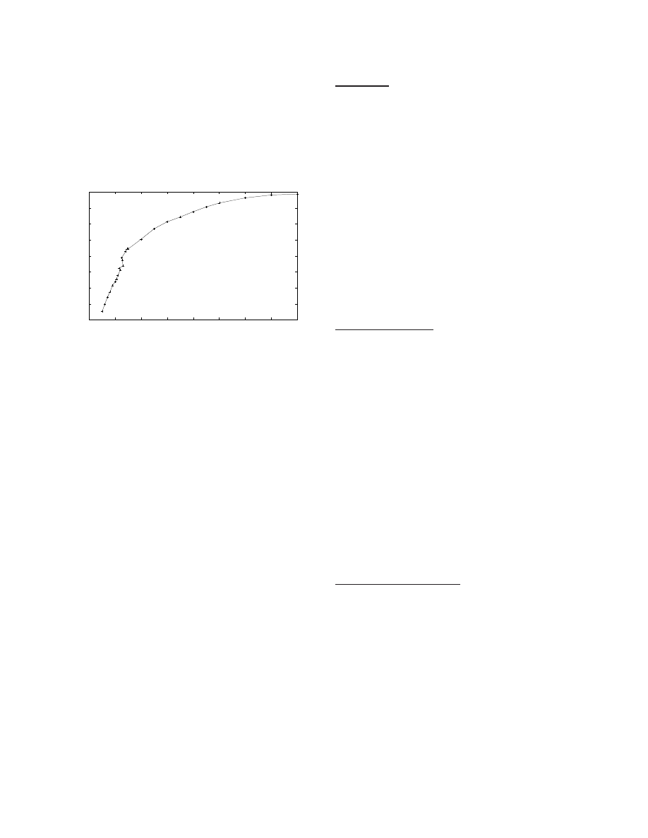
Figure 3: Number of neurons firing at each simulation time step. A The graph shows the first 1000 simulation steps of a
model G(65536, 880) with 57.67 million neurons using 32, 768 processors. The average neuronal firing rate was 7.2 Hz while
the stimulus was random at 6 Hz. A rhythmic oscillatory pattern can be clearly seen with a peak around 1.4 million (roughly,
2.42% of all neurons).

duction in the number of messages by a factor of 80. Fur-
thermore, when a neuron n on processor x fires, we do not
instantly send the message to every processor that the neu-
ron connects to; rather, we aggregate (piggy-back) multiple
firings of neurons whose axons also travel from processor x
to processor y in a single message. This reduces communica-
tion overhead. As the average neuronal firing rate increases,
the advantage of this optimization increases further. Step
FlshMsg

cleans up any remaining messages which have not

yet become full after all neurons have been processed. Steps
NrnUpd

and FlshMsg keep track of how many messages

are sent from processor x to any given processor y in variable
M

x

(y). All messages are sent in a non-blocking fashion.

Observe how the messages are sent in NrnUpd and FlshMsg
before local computation in Step PSTDP proceeds. By de-
laying computation in PSTDP which can be also placed
between NrnUpd and FlshMsg, we allow communication
to overlap computation, thus hiding communication latency.

Finally, in Step MeX1, by using MPI ReduceScatter, we fig-
ure out for each processor x the number of incoming mes-
sages that it expects to receive. This trick removes all am-
biguity from message exchanges. Now, in Step MeX2, pro-
cessor x simply receives M (x) =

P

N
y=1

M

y

(x) messages that

it is expecting in a blocking fashion. As explained in the in-
troduction, steps MeX1 and MeX2 are a key feature of our
algorithm, and they significantly reduce the communication
and synchronization costs.

After receiving the messages, in Step N1, we set up appro-
priate events in the future so as to activate relevant synapses
as per the applicable axonal delay. In essence, Step N1 of
Figure 1 is now represented by Step NrnUpd (Part(c)),
FlshMsg

, MeX1, MeX2, and N1 of Figure 2.

4.

MODELS AND METHODS

4.1

Network Models

To benchmark the simulator, we developed a range of net-
work models that are easily parameterized so as to enable
extensive testing and analysis. Like the cortex, all our mod-
els have roughly 80% excitatory and 20% inhibitory neu-
rons with 8, 000 synapses on an average.

The networks

are not structured to be neuro-anatomically plausible, but
are interconnected in a probabilistic fashion. Our largest
rat-scale model also satisfies an important empirical con-
straint, namely, it has a local connection probability of 0.09
[3, Chapter 20]. Such a choice of network is consistent with
other evaluations of cortical simulators [4, 14, 18]. For in-
stance, [18] used 100,000 neurons each with 10,000 random
synaptic connections.

We assume that inhibitory neurons can connect only to exci-
tatory neurons, while excitatory neurons can connect to ei-
ther type. Let H(α, β, γ, δ) denote a random directed graph
with α vertices and β outgoing edges per vertex. Each ver-
tex represents a group of γ neurons. The total number of
neurons is α × γ. A group of neurons does not have any
biological significance. There are α × 0.8 excitatory groups
and α×0.2 inhibitory groups. Each excitatory group sends β
edges randomly to one of the α groups, while each inhibitory
group sends β edges randomly to one of the α×0.8 excitatory
groups. Each edge originating from an excitatory group has
an integer axonal delay chosen randomly from the interval
[1, δ], while each edge originating from an inhibitory group
has a fixed axonal delay of 1 ms. If there is a directed edge
from group G1 to G2, then a neuron in group G1 connects
with a neuron in group G2 with probability 8000/(β × γ).
In this paper, we set β = 100 and δ = 20 ms. For brevity,
we write G(α, γ) ≡ H(α, 100, γ, 20). We will use ten differ-
ent models by varying α (the number of groups) and γ (the

0

200

400

600

800

1000

1200

1400

1600

1800

0

200

400

600

800

1000

Neuron ID

Simulation Time Step

Neuron Raster

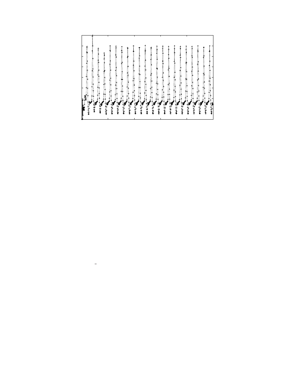
Figure 4: Raster plot of selected neurons for the first 1000 simulation steps of a model G(4096, 110) with 450, 560 neurons using
256 processors. The plot corresponds to 16 groups comprising 1, 760 neurons assigned to processor 0. Similar results have
been observed in other neurons. The four groups comprising the top quarter of the graph are inhibitory, the rest comprising
the bottom three-quarters of the graph are excitatory. In this graph, a dot is plotted at (t, n) if a neuron n fires at time step
t (the count of all such dots on all processors at a given time would yield a firing rate plot similar to Figure 3). The graph
shows that the inhibitory groups have a visibly higher firing rate than excitatory groups, as evidenced by the density of the
dots. Neuronal firing occurs in a fairly synchronized manner, but involve different groups at different times. Some groups
exhibit aperiodic behavior as exemplified by Group 12 (neurons between the two horizontal lines).

number of neurons per group). To see a list of all the groups,
refer to the bottom row of the label on the x-axis in Figure
5. To obtain a larger problem size, the number of neurons
is increased through a combination of increased number of
groups and number of neurons per group.

4.2

Operating Point and Cortical Dynamics

The dynamics of the cortical networks depend upon many
parameters such as neuronal dynamics, synaptic dynamics,
network topology, nature and frequency of external stimu-
lation, constants W

+

, A

+

and A

−

, etc. A comprehensive

study of network dynamics is outside the scope of this work.
For all simulations, we have used a stable rhythmic regime of
the network [28], as illustrated in Figures 3 and 4. Further,
we have used a regime that produces an effective average
neuronal firing rate higher than the stimulus rate.

To achieve this regime, various network parameters were
chosen as follows. The event horizon δ = 20 ms. The con-
stants in (1) and (2) are set as τ

−

= 20 ms, A

−

= 0.00264,

τ

+

= 20 ms, and A

+

= 0.0022. The weights of plastic

synapses made by excitatory neurons are upper bounded by
W

+

= 0.22 mV. The weights of non-plastic synapses made

by inhibitory neurons are set to W

−

= −0.11 mV. We used

the four parameter phenomenological, single-compartment
neurons in [15, 14]; we used [a = 0.02, b = 0.2, c = −65, d =
8] corresponding to regular spiking for the excitatory neu-
rons and [a = 0.1, b = 0.2, c = −65, d = 2] corresponding
to fast spiking for the inhibitory neurons. We use instanta-
neous (memoryless or delta function) synapses [10].

All our models (except those in Section 5.5) use a random
stimulus probability of 6 Hz meaning that at each simulation
time step of 1 ms each neuron was given a super-threshold
stimulus of 20 mV with probability 0.006. This results in
an average neuronal firing rate of roughly 7.2 Hz. All sim-
ulations are run for 5 seconds of model time (5, 000 time
steps).

4.3

Layout of a Model on Processors

All neurons in a group are always placed on the same pro-
cessor. Different groups may also be collocated on the same
processor. To achieve load balancing in computation and
memory, we place the same number of groups on each proces-
sor so as to keep the total number of neurons per processor
to 1, 760. Furthermore, to achieve load balancing in commu-
nication and memory, we try to assign groups to processors
such that variability in the number of processors connected
to any given processor is reduced. Finally, in our models,
although only 1 in 5 neurons is inhibitory, 60% of all fir-
ing is inhibitory. Hence, it is also important to balance the
inhibitory neurons among the processors in order to reduce
variability in firing across processors.

5.

SIMULATION RESULTS

5.1

Memory Usage

For various models used across several processor configura-
tions, synapses consume an overwhelming majority of the
memory, roughly, 84%. Recall that in our model the axon
of a neuron may travel to multiple processors, and that on
each processor we must store all the synapses that the axon
makes; thus, the size of this data structure increases with

0

10

20

30

40

50

60

64

1K,110

128

1K,220

256

4K,110

512

4K,220

1024

4K,440

2048

32K,110

4096

32K,220

8192

32K,440

16384

64K,440

32768

64K,880

Model Size (Number of Neurons, millions)

Top Row: Number of CPUs; Bottom Row: Groups (K=1024), Neurons per Group

Model Size Scaling

Number of Neurons

Mouse-scale Cortex

Rat-scale Cortex

Figure 5: Maximum number of neurons with 8, 000 synapses each (on an average) that can fit in the memory available in
a given number of processors with 1, 760 neurons per processor. The graph shows that the maximum number of neurons is
doubled when twice the number of processors are available; and, hence, that C2 makes an efficient use of the available memory.

the model size, the number of groups, and increasing num-
ber of connections that a processor makes. For the largest
(smallest) model, it consumes about 6% (3%) of the memory.
More importantly, the amount of transient memory used for
data structures to store delayed neuronal firing events and
message buffers is a small fraction (less than 1%), even for
the largest model, which is a key consideration for a compu-
tation that is inherently message-bound.

5.2

Main Results

Figure 5 shows that C2 is capable of fully exploiting the
larger memory available with increasing number of proces-
sors by accommodating progressively larger models. The
key point is that we can represent mammalian-scale cortical
models at mouse-scale [2] and rat-scale.

Figure 6 shows simulation run-time as a function of the num-
ber of processors while using progressively larger models.
The key point is that 1 second of model time can be simu-
lated in less than 10 seconds at 1 Hz average neuronal firing
rate, even for the largest model. In general, this plot con-
firms the goal that the simulator achieves a realistic turn-
around time for large models, essential for studying model
dynamics over a variety of parameters.

An interesting statistics is that on the rat-scale model, 16.6×
10

12

spikes were processed in 325 seconds on 32, 768 proces-

sors.

5.3

Simulation Time: A Deeper Analysis

We now ask what causes the simulation run-time to in-
crease with larger models on larger number of processors.
To this end, Figure 7 shows break-down of run-time in terms
of components SynAct+DSTDP, NrnUpd, FlshMsg,
PSTDP

, and MeX delineated in Figure 2. There are sev-

eral key observations.

First, for larger models MeX component dominates, and,
hence, without our optimizations, such large-scale simula-
tions would have been impossible.

Second, only the MeX component increases with increas-
ing number of processors while the other components scale
essentially perfectly. The increasing cost of MeX is due to
the fact that number of messages increases faster than the
number of spikes delivered, due to the increasing number of
groups used in larger models; see Figure 8.

Third, recall that PSTDP and FlshMsg can overlap –
thus hiding communication latency. Whereas the PSTDP
component is relatively constant per processor, the number
of messages per processor increases (as seen in Figure 8).
And, hence, as larger number of processors and progressively
larger models are used, eventually, the rise in number of
messages causes a relative rise in FlshMsg component.

Fourth, time taken for neuronal updates, NrnUpd, is neg-
ligible when compared to SynAct+DSTDP+ PSTDP,
that is, synaptic updates dominate computation time. Re-
call that PSTDP operates only over the list of recently
activated synapses. In our simulations, the size of this list is
around 2, 200 which is much smaller than the average num-
ber of synapses per neuron, namely, 8, 000. Although not
addressed here, the reduction of the accessed synaptic mem-
ory foot-print will be pre-requisite for cache optimizations.

5.4

Strong Scaling

So far, for a given number of processors, we have focussed
on using models that are memory-bound. We now relax
this constraint, and study the effect on simulation run-time
for a fixed model with increasing number of processors as
shown in Figure 9. The key lesson is that for larger models
as the number of processors are increased (thus decreasing

0

50

100

150

200

250

300

350

64

1K,110

128

1K,220

256

4K,110

512

4K,220

1024

4K,440

2048

32K,110

4096

32K,220

8192

32K,440

16384

64K,440

32768

64K,880

0

1

2

3

4

5

6

7

8

9

10

Run-time (in seconds)

Run-time per Model Second per Hz (in seconds)

Top Row: Number of CPUs; Bottom Row: Groups (K=1024), Neurons per Group

Run-time Scaling

(Model time = 5 seconds)

Run-time

Normalized Run-time

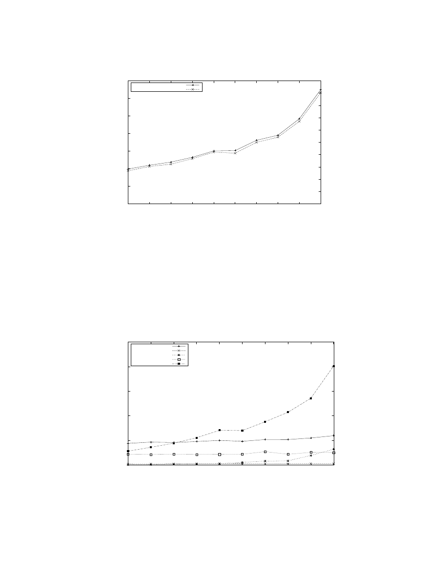
Figure 6: Relationship between total simulation run-time and number of processors used where a correspondingly larger model
is used for larger number of processors. The run-time depends on the number of model seconds simulated, the firing rate, and
the dynamics of the interaction between groups (for example, messages exchanged). The second plot (with right y-axis) shows
the normalized run-time which is the time taken to simulate 1 model second at 1 Hz firing rate. Both plots show that the
run-time increases only 3 times when the number of processors and the number of neurons are scaled 512 fold, respectively,
from 64 to 32, 768 and 112, 640 to 57, 671, 680.

0

50

100

150

200

250

64

1K,110

128

1K,220

256

4K,110

512

4K,220

1024

4K,440

2048

32K,110

4096

32K,220

8192

32K,440

16384

64K,440

32768

64K,880

Component run-time (in seconds)

Top Row: Number of CPUs; Bottom Row: Groups (K=1024), Neurons per Group

Run-time Scaling - Break-down

(Model time = 5 seconds)

SynAct + DSTDP

NrnUpd

FlshMsg

PSTDP

MeX1 + MeX2

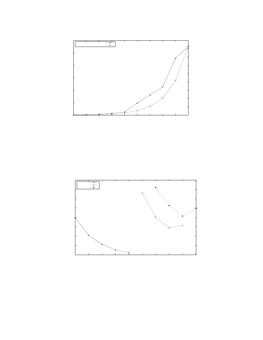
Figure 7: Break-down of time taken for simulation (run-time) for different number of processors used in terms of different
components of the algorithm in Figure 2.

0

5

10

15

20

25

30

64

1K,110

128

1K,220

256

4K,110

512

4K,220

1024

4K,440

2048

32K,110

4096

32K,220

8192

32K,440

16384

64K,440

32768

64K,880

0

2

4

6

8

10

12

14

16

18

Number of Messages (in billions)

Number of Spikes (in trillions)

Top Row: Number of CPUs; Bottom Row: Groups (K=1024), Neurons per Group

Number of Messages and Spikes

Number of Messages

Number of Spikes

Figure 8: Total number of messages exchanged and spikes delivered. The number of spikes essentially doubles while the number
of processors (and, correspondingly, the model size) is doubled (Figure 5); and, hence, across all models and processors, the
average number of spikes per processor is roughly a constant. The number of messages, however, increases faster than the
number of spikes delivered, due to the increasing number of groups used in the different models. This contributes to the
increase in the cost of the MeX component with larger models simulated on increasing number of processors.

20

40

60

80

100

120

140

160

180

64

128

256

512

1024

2048

4096

8192

16384

32768

Run-time (in seconds)

Number of CPUs

Strong Scaling

Model 1
Model 2
Model 3

Figure 9: Simulation run-time for 3 different models with increasing number of processors over 5 second of model time.
Model 1 uses G(1024, 110) with 112, 640 neurons, Model 2 uses G(32768, 110) with 3, 604, 480 neurons, and Model 3 uses
G(32768, 220) with 7, 208, 960 neurons. The plot for Model 1 shows moderate scaling in run-time as more processors are made
available, until the number of groups equals the number of processors. This is due to the relatively smaller proportion of the
MeX

component for 1024 group at 64 processors, the starting point, as seen in Figure 7. In contrast, the MeX component

becomes dominant at larger number of processors and model sizes. Thus, the plots for Models 2 and 3 initially show a decrease
in run-times but eventually exhibit a worsening in run-times, at 16, 384 and 32, 768 processors, respectively.

the pressure on computational resources), the simulations
become communication-bound.

5.5

Effect of Firing Rate

Until now, we have fixed the stimulus probability. We now
vary the stimulus probability and study its effect on the
average neuronal firing rate; see Figure 10. There are several
key observations.

5

6

7

8

9

10

11

12

13

4

6

8

10

12

14

16

18

20

Firing Rate (Hz)

Stimulus Probability (Hz)

Stimulus vs. Firing Rate

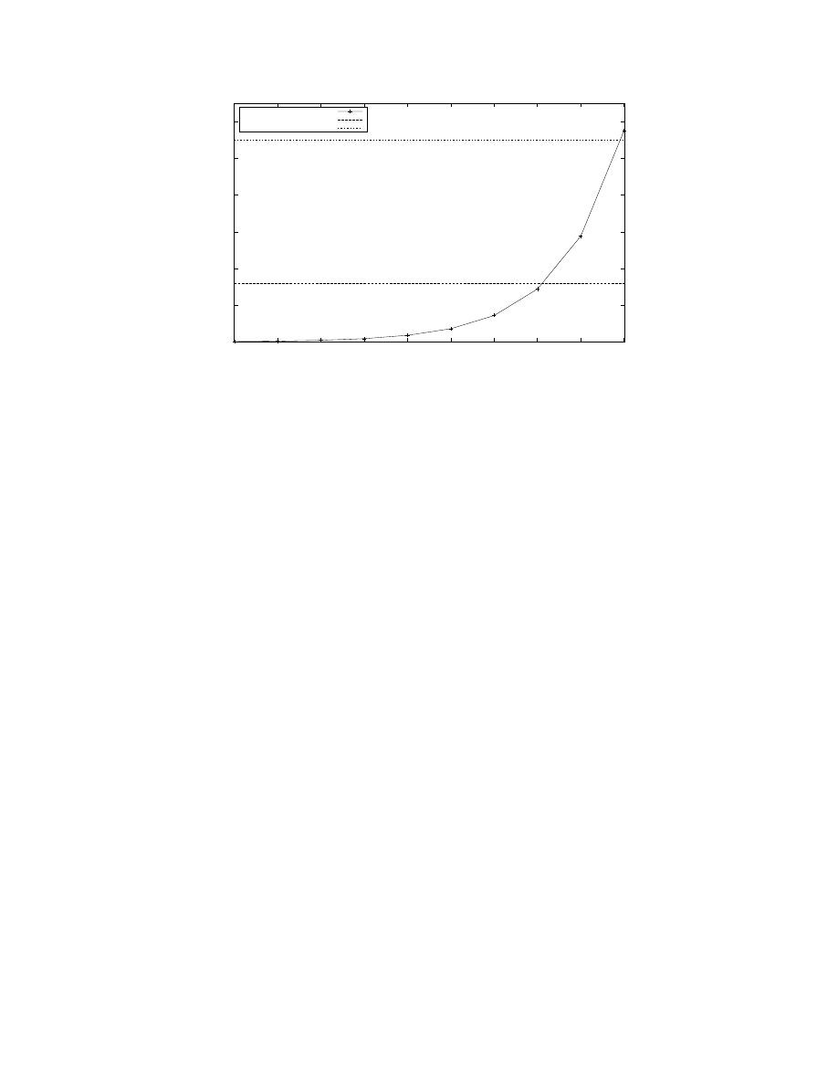
Figure 10: Average neuronal firing rate as a function of the
stimulus probability for model G(1024, 110) with 112, 640
neurons on 64 processors.

First, the cost of simulation increases with an increase in
the average neuronal firing rate. Further analysis shows that
components SynAct+DSTDP and PSTDP, increase lin-
early in run-time with increasing average firing rate. Addi-
tionally, the cost of MeX component depends on how the
neuronal firings are distributed across different processors
as a function of simulation time steps. If the distribution is
even across the processors and through time, then the cost
of MeX tends to be low, but as the distribution becomes
skewed the cost increases.

Second, as the average firing rate increases, the total num-
ber of spikes delivered increases linearly. However, with in-
creasing firing rate there is a higher probability that multi-
ple neurons on a source processor that connect to the same
target processor fire within the same time step; this leads
to an increased opportunity for message aggregation (piggy-
backing), and, hence, the total number of messages increases
only sub-linearly.

Third, recall that, for every neuron n, we put all synapses
that are activated between consecutive neuronal firings on
a list R(n). For the model in Figure 10, the size of this
list varies between 2, 200 and 2, 400, and is still significantly
smaller than 8, 000 which is the average number of synapses.
When a neuron fires, all synapses on the list R(n) for that
neuron that were activated within the previous 250 ms (∆ <
250) are potentiated. These potentiated synapses are a sub-
set of R(n). The percentage of this subset varies from about
90% for lower firing rates to almost 100% for higher firing
rates, meaning that as neurons fire more frequently more of
the synapses are rewarded.

6.

DISCUSSION AND CONCLUSIONS

Significance: We have presented the construction and eval-
uation of a powerful tool, C2, to explore the computational
function of the cortex. To summarize, by combining state-
of-the-art hardware with innovative algorithms and software
design, we are able to simultaneously achieve unprecedented
time-to-solution on an unprecedented problem size.

These results represent a judicious intersection between com-
puter science which defines the region of feasibility in terms
of available computing resources today, and neuroscience
which defines the region of desirability in terms of biolog-
ical details that one would like to add. At any given point
in time, to get a particular scale of simulation at a partic-
ular simulation speed, one must balance between feasibility
and desirability. Thus, our results demonstrate that a non-
empty intersection between these two regions exists today
at rat-scale, at near real-time and at a certain complexity of
simulations. This intersection will continue to expand over
time. As more biological richness is added, correspondingly
more resources will be required to accommodate the model
in memory and to maintain reasonable simulation times.

Enriching Simulations: Here, we have focussed on simula-
tions that can easily be scaled in terms of number of neurons
and synapses to benchmark the performance of C2 on vary-
ing number of processors. In future, we will employ C2 for
understanding and harnessing dynamics of such large-scale
spiking networks for information processing; for a first step,
see [2]. These networks exhibit extremely complex dynamics
that is hard to encapsulate in just a few measurable values
such the firing rate, etc., and, hence, to facilitate a deeper
understanding, we are building tools to visualize the state of
the simulation as it evolves through time. We will also en-
rich simulations by incorporating numerous neurobiological
details and constraints such as white matter [24] and gray
matter connectivity, neuromodulators, thalamocortical and
corticothalamic connections, and dynamic synapses. Specif-
ically, we will focus on those details that are relevant to
understand how various neurobiolgical details affect the dy-
namical, operational, computational, information process-
ing, and learning capacity of the cortical simulator. Finally,
with a view towards applications, we are interested in ex-
perimenting with a wide array of synthetic and real spatio-
temporal stimuli.

Need for Novel Architectures: The cortex is an analog, asyn-
chronous, parallel, biophysical, fault-tolerant, and distributed
memory machine. C2 represents one logical abstraction of
the cortex that is suitable for simulation on modern dis-
tributed memory multiprocessors. Computation and mem-
ory are fully distributed in the cortex, whereas in C2 each
processor houses and processes several neurons and synapses.
Communication is implemented in the cortex via targeted
physical wiring, whereas in C2 it is implemented in software
by message passing on top of an underlying general-purpose
communication infrastructure. Unlike the cortex, C2 uses
discrete simulation time steps and synchronizes all proces-
sors at every step. In light of these observations, the search
for new types of (perhaps non-von Neumann) computer ar-
chitecture to truly mimic the brain remains an open question
[29]. However, we believe that detailed design of the simu-
lator and analysis of the results presented in this paper may

present one angle of attack towards this quest.

Coda: Our long-term goals are to develop novel brain-like
computing architectures along with appropriate program-
ming paradigms, and to evolve C2 into a cortex-like uni-
versal computational platform that integrates and opera-
tionalizes existing quantitative neuroscientific data to build
a powerful learning machine: a cognitive computer [8].

Acknowledgments

We are grateful to the executive management at IBM’s Al-
maden Research Center, namely, Dr. Mark Dean, Dr. Dilip
Kandlur, Dr. Laura Haas, Dr. Gian-Luca Bona, Dr. James
Spohrer, and Dr. Moidin Mohiuddin, for their vision in initi-
ating and supporting the Cognitive Computing grand chal-
lenge project. For experiments, we used the BlueGene/L
machines at IBM’s Almaden and Watson Research Labs.

7.

REFERENCES

[1] G. Alm´

asi et al. Optimization of MPI collective

communication on BlueGene/L systems. In Int. Conf.
Supercomputing, pages 253–262, 2005.

[2] R. Ananthanarayanan and D. S. Modha. Scaling,

stability, and synchronization in mouse-sized (and
larger) cortical simulations. In CNS*2007. BMC
Neurosci., 8(Suppl 2):P187, 2007.

[3] V. Braitenberg and A. Sch¨

uz. Cortex: Statistics and

Geometry of Neuronal Conectivity. Springer, 1998.

[4] R. Brette et al. Simulation of networks of spiking

neurons: A review of tools and strategies. J. Comput.
Neurosci. (submitted), 2006.

[5] E. Chan, R. van de Geijn, W. Gropp, and R. Thakur.

Collective communication on architectures that
support simultaneous communication over multiple
links. In PPoPP, pages 2–11, 2006.

[6] P. Dayan and L. F. Abbott. Theoretical Neuroscience:

Computational and Mathematical Modeling of Neural
Systems. MIT Press, 2005.

[7] A. Delorme and S. Thorpe. SpikeNET: An

event-driven simulation package for modeling large
networks of spiking neurons. Network: Comput.
Neural Syst., 14:613:627, 2003.

[8] G. M. Edelman. Second Nature: Brain Science and

Human Knowledge. Yale University Press, 2006.

[9] B. G. Farley and W. A. Clark. Simulation of

self-organizing systems by digital computer. IRE
Trans. Inform. Theory, IT-4:76–84, September 1954.

[10] N. Fourcaud and N. Brunel. Dynamics of the firing

probability of noisy integrate-and-fire neurons. Neural
Comput., pages 2057–2110, 2002.

[11] A. Gara et al. Overview of the Blue Gene/L system

architecture. IBM J. Res. Devel., 49:195–212, 2005.

[12] W. Gropp, E. Lusk, and A. Skjellum. Using MPI:

Portable Parallel Programming with the Message
Passing Interface. MIT Press, Cambridge, MA, 1996.

[13] S. Hill and G. Tononi. Modeling sleep and wakefulness

in the thalamacortical system. J. Neurophysiol.,
93:1671–1698, 2005.

[14] E. M. Izhikevich. Polychronization: Computation with

spikes. Neural Comput., 18:245–282, 2006.

[15] E. M. Izhikevich, J. A. Gally, and G. M. Edelman.

Spike-timing dynamics of neuronal groups. Cerebral
Cortex, 14:933–944, 2004.

[16] C. Johansson and A. Lansner. Towards cortex sized

artificial neural systems. Neural Networks,
20(1):48–61, 2007.

[17] M. Mattia and P. D. Guidice. Efficient event-driven

simulation of large networks of spiking neurons and
dynamical synapses. Neural Comput., 12:2305–2329,
2000.

[18] A. Morrison, C. Mehring, T. Geisel, A. D. Aertsen,

and M. Diesmann. Advancing the boundaries of
high-connectivity network simulation with distributed
computing. Neural Comput., 17(8):1776–1801, 2005.

[19] R. Nieuwenhuys, H. J. ten Donkelaar, and

C. Nicholson. Section 22.11.6.6; Neocortex:
Quantitative aspects and folding. In The Central
Nervous System of Vertebrates, volume 3, pages
2008–2013. Springer-Verlag, Heidelberg, 1997.

[20] N. Rochester, J. H. Holland, L. H. Haibt, and W. L.

Duda. Tests on a cell assembly theory of the action of
the brain using a large digital computer. IRE Trans.
Inform. Theory, IT-2:80–93, September 1956.

[21] A. J. Rockel, R. W. Hirons, and T. P. S. Powell.

Number of neurons through the full depth of the
neocortex. Proc. Anat. Soc. Great Britain and Ireland,
118:371, 1974.

[22] E. Ros, R. Carrillo, E. Ortigosa, B. Barbour, and

R. Ag´ıs. Event-driven simulation scheme for spiking
neural networks using lookup tables to characterize
neuronal dynamics. Neural Comput., 18:2959–2993,
2006.

[23] A. Sch¨

uz and G. Palm. Density of neurons and

synapses in the cerebral cortex of the mouse. J. Comp.
Neurol., 286:442–455, 1989.

[24] R. Singh, S. Hojjati, and D. S. Modha. Interactive

visualization and graph analysis of CoCoMac’s brain
parcellation and white matter connectivity data. In
SfN: Society for Neuroscience, November 2007.

[25] M. Snir, S. W. Otto, S. Huss-Lederman, D. W.

Walker, and J. Dongarra. MPI: The Complete
Reference. MIT Press, Cambridge, MA, 1997.

[26] S. Song, K. D. Miller, and L. F. Abbott. Competitive

Hebbian learning through spike-timing-dependent
synaptic plasticity. Nature Neurosci., 3:919-926, 2000.

[27] R. Thakur, R. Rabenseifner, and W. Gropp.

Optimization of collective communication operations
in MPICH. Int. J. High Perf. Comput. App.,
19(1):49–66, 2005.

[28] T. P. Vogels, K. Rajan, and L. F. Abbott. Neural

network dynamics. Annu. Rev. Neuroscience,
28:357–376, 2005.

[29] J. von Neumann. The Computer and The Brain. Yale

University Press, 1958.

[30] L. Watts. Event-driven simulation of networks of

spiking neurons. In NIPS, volume 6, pages 927–934,
1994.