Computer Virus Propagation Models

Giuseppe Serazzi and Stefano Zanero

?

Dipartimento di Elettronica e Informazione, Politecnico di Milano,

Via Ponzio 34/5, 20133 Milano, Italy,

[e-mail], [e-mail]

Abstract. The availability of reliable models of computer virus propa-
gation would prove useful in a number of ways, in order both to predict
future threats, and to develop new containment measures. In this pa-
per, we review the most popular models of virus propagation, analyzing
the underlying assumptions of each of them, their strengths and their
weaknesses. We also introduce a new model, which extends the Random
Constant Spread modeling technique, allowing us to draw some conclu-
sions about the behavior of the Internet infrastructure in presence of a
self-replicating worm. A comparison of the results of the model with the
actual behavior of the infrastructure during recent worm outbreaks is
also presented.

1

Introduction

The concept of a computer virus is relatively old, in the young and expanding
field of information security. First developed by Cohen in [1] and [2], the concept
of “self-replicating code” has been presented and studied in many researches,
both in the academic world and in the so-called “underground”. The spread of
computer viruses still accounts for a significant share of the financial losses that
large organizations suffer for computer security problems [3].

While many researches deal with concept such as the creation of new viruses,

enhanced worms and new viral vectors, or the development of new techniques
for detection and containment, some effort has been done also in the area of
modeling viral code replication and propagation behavior. The importance of
this work, and the shortcomings of many existing models, are described in [4].

Creating reliable models of virus and worm propagation is beneficial for many

reasons. First, it allows researchers to better understand the threat posed by new
attack vector and new propagation techniques. For instance, the use of concep-
tual models of worm propagation allowed researchers to predict the behavior
of future malware, and later to verify that their predictions were substantially
correct [5].

In second place, using such models, researchers can develop and test new and

improved models for containment and disinfection of viruses without resorting

?

Work partially supported by IEIIT-CNR institute, and COFIN 2001-Web and FIRB-
Perf projects.

to risky “in vitro” experimentation of zoo virus release and cleanup on testbed
networks [6].

Finally, if these models are combined with good load modeling techniques

such as the queueing networks, we can use them to predict failures of the global
network infrastructure when exposed to worm attacks. Moreover, we can indi-
viduate and describe characteristic symptoms of worm activity, and use them as
an early detection mechanism.

In order to be useful, however, such a model must exhibit some well-known

characteristics: it must be accurate in its predictions and it must be as general
as possible, while remaining as simple and as low-cost as possible.

In this paper we present a critical review of most of the existing models of

virus propagation, showing the underlying assumptions of each of them, and their
strengths and weaknesses. We also introduce a new model, based on the same
foundations of an existing technique, which allows us to draw some conclusions
about the stability of the Internet infrastructure in presence of a self-replicating
worm. We compare our modeling results with actual behavior of the infrastruc-
ture during recent worm crises and show that our model can accurately describe
some effects observed during fast worms propagation.

2

A survey of existing modeling techniques

Viral code propagation vectors have evolved over the years. In the beginning
of the virus era, the most common vector of propagation was the exchange of
files via floppy disks and similar supports. The pathogens were viruses, in the
strictest sense: they propagated by appending their code to a host program,
which had to be executed in order to spread the infection, and to execute the
payload if present. This applies, with some modification, also to the so-called
“boot sector viruses” which infected the boot loader of the operating system,
and spread by infecting the boot sector of floppy disks, which would run whenever
a disk was unintentionally left in the machine at boot time. The same concept,
in more recent times, has been extended to macro languages embedded in office
automation suites, generating the so-called “macro viruses”.

The concept of a worm, i.e. a self-contained, self-propagating program which

did not require an host program to be carried around, was also developed, but
was somehow neglected for a long time. In 1988, however, the Internet Worm
[7] changed the landscape of the threats. The Internet Worm was the first suc-
cessful example of a self-propagating program which did not infect host files,
but was self contained. Moreover, it was the first really successful example of
an active network worm, which propagated on the Internet by using well-known
vulnerabilities of the UNIX operating system. Other worms used open network
shares, or exploited vulnerabilities in operating systems and server software to
propagate.

With the widespread adoption of the Internet, mass-mailing worms began to

appear. The damage caused by Melissa virus in 1999, Love Letter in 2000 and
Sircam in 2001 demonstrated that tricking users into executing the worm code

M Passive immunity

S

Susceptible state

E Exposed to infection

I

Infective

R

Recovered

Table 1. Typical states for an epidemiological model

attached to an e-mail, or exploiting a vulnerability in a common e-mail client to
automatically launch it, is a successful way to propagate viral code.

Each of these different propagation vectors has inspired various propagation

models. In the next sections, we will review the most interesting and successful
models for each class: file, macro and boot sector viruses, e-mail based worms,
“active” (or “scanning”) Internet worms.

It is important to note that modern viruses often use a mix of these techniques

to spread (for instance, Sircam uses both mass mailing and open network shares,
while Nimda uses four different mechanisms to propagate). We are not aware,
however, of any existing model which takes into account multi-vector viruses
and worms. So, we will follow a traditional taxonomy in presenting the existing
modeling techniques.

2.1

Modeling traditional viruses

The first complete application of mathematical models to computer virus prop-
agation appeared in [8]. The basic intuitions of this work still provide the fun-
damental assumptions of most computer epidemiological models.

Epidemiological models abstract from the individuals, and consider them

units of a population. Each unit can only belong to a limited number of states
(e.g. “susceptible” or “infected”; see Table 1 for additional states): usually, the
chain of these states gives the name to the model, e.g., a model where the
Susceptible population becomes Infected, and then Recovers, is called a SIR
model, whereas a model with a Susceptible population which becomes Infected,
and then goes back to a Susceptible state is called SIS.

Another typical simplification consists in avoiding a detailed analysis of virus

transmission mechanics, translating them into a probability that an individual
will infect another individual (with some parameters). In a similar way, transi-
tions between other states of the model are described by simple probabilities.
Such probabilities could be calculated directly by the details of the infection
mechanism or, more likely, they can be inferred by fitting the model to actual
propagation data. An excellent analysis of mathematics for infectious diseases
in the biological world is available in [9].

Most epidemiological models, however, share two important shortcomings:

they are homogeneous, i.e. an infected individual is equally likely to infect any
other individual; and they are symmetric, which means that there is no priv-
ileged direction of transmission of the virus. The former makes these models

unappropriate for illnesses that require a non-casual contact for transmission;
the latter constitutes a problem, for instance, in the case of sexually-transmitted
diseases.

In the case of computer viruses, however, both problems are often grievous.

For example, most individuals exchange programs and documents (by means of
e-mails or diskettes) in almost closed groups, and thus an homogeneous model
may not be appropriate. Furthermore, there are also “sources” of information
and programs (e.g. computer dealers and software distributors) and “sinks” (final
users): that makes asymmetry a key factor of data exchange.

In [8] both these shortcomings are addressed by transferring a traditional SIS

model onto a directed random graph, and the important effects of the topology of
the graph on propagation speed are analyzed. The authors describe the behavior
of virus infections on sparse and local graphs. In a sparse graph, each node has a
small, constant average degree; on the contrary, in a local graph, the probability
of having a vertex between nodes B and C is significantly higher if both have a
vertex connected to the same node A. The authors discuss that in the landscape
of the beginnings of the 90s the latter situation approximated very well the
interaction between computer users. Among other results, it is shown that the
more sparse a graph is, the slower is the spread of an infection on it; and the
higher is the probability that an epidemic condition does not occur at all, which
means that sparseness helps in containing global virus spread (while local spread
is unhindered). Further elaborations on this type of model can be found in [10].

These findings are useful and interesting. However, it must be noted that

often a SIR model, in which a “cured” system is not susceptible any more,
could approximate better the behavior of many real cases of propagation when
a patch or antivirus signature is available. Also, the introduction of the Internet
as a convenient and immediate way for software and data exchange has arguably
made the assumptions of locality and sparseness of the graph no longer valid.

2.2

Modeling e-mail based worms

In a technical report [11] Zou et al. describe a model of e-mail worm propa-
gation. The authors model the Internet e-mail service as an undirected graph
of relationship between people (i.e. if user A has user B’s e-mail address in his
address book, B has probably A’s address in her contacts also). In order to build
a simulation of this graph, they assume that each node degree is distributed on
a power-law probability function.

They draw this assumption from the analysis of “Yahoo!” discussion group

sizes, which result to be heavy-tailed. Since once a user puts a discussion group
address in his contact book he actually adds an edge toward all the group mem-
bers, the node degree should be heavy-tailed too. It is unclear if this distribution
reflects also the true distribution of contacts (i.e. not considering e-mail lists)
among Internet users. However, considering that nowadays most Internet dis-
cussion groups employ content filtering or ban attachments altogether, they are
not a very viable virus propagation vector. The construction method, based
on a “small world” network topology, seems to ignore completely the existence

of interest groups and organizations, which naturally create clusters of densely
connected vertices.

Furthermore, the authors assume that each user “opens” an incoming virus

attachment with a fixed probability P

i

, a function of the user but constant in

time. This does not describe very well the typical behavior of users. Indeed, most
experienced users avoid virus attachments altogether, while unexperienced users
open them every time, thus making this approximation misleading.

They model e-mail checking time T

i

as either an exponentially or Erlang

distributed random variable. The means of these distributions, T = E[T

i

], and

P = E[P

i

] are assumed to be independently distributed gaussians.

An interesting observation the authors make is that since the user e-mail

checking time is much larger than the average e-mail transmission time, the
latter can be disregarded in the model. The authors proceed in considering a
“reinfection” model, where a user will send out copies of the e-mail virus each
time he reopens an infected attachment, as opposed to a “non-reinfection” model
where this happens just once. Neither model is very realistic: in many cases, e-
mail viruses install themselves as startup services on the system, and spread
themselves at each opportunity.

These observations suggest that the results of the simulation should be con-

sidered as qualitative, rather than quantitative, indications. A couple of inter-
esting points can be drawn from this study. Firstly, infecting users with high
“degrees”, i.e. an high number of contacts, in the early phase of infection speeds
up the process considerably (and conversely, making these nodes immune to
the virus helps defending against it). A second observation is that the overall
spread rate of viruses gets higher as the variability of users’ e-mail checking times
increases.

2.3

Modeling a scanning worm: The Random Constant Spread
model

The Random Constant Spread (RCS) model [5] was developed by Staniford,
Paxson and Weaver using empirical data derived from the outbreak of the Code
Red worm. This worm was released in its first version (which we will call CRv1)
onto the Internet on July 13th 2001, according to the initial analysis from eEye
Digital Security [12]. The CRv1 worm was disassembled and studied quickly [13],
making its diffusion mechanism very clear.

Code Red propagates by using the .ida vulnerability discovered by eEye it-

self on June 18th 2001 [14], thus infecting vulnerable web servers running Mi-
crosoft IIS version 4.0 and 5.0. When Code Red infects an host, it spreads by
launching 99 threads, which randomly generate IP addresses (excluding subnets
127.0.0.0/8, loopback, and 224.0.0.0/8, multicast) and try to compromise the
hosts at those addresses using the same vulnerability.

CRv1, however, had a fundamental design flaw: the random number gener-

ator of each thread was initialized with a fixed seed, so all the copies of the
worm in a particular thread, on all infected hosts, generated the same sequence
of target IP addresses, attempting to compromise them in that fixed order. The

thread identifier is used as part of the seed, so each instance of the worm has 99
different sequences, but these sequences were the same for all the instances of
the worm. For this reason, CRv1 was not very effective nor dangerous: since all
the instances of the worm scanned the same sequence of IP addresses, the worm
spread was only linear.

A particularity of this worm is that it does not reside on the file system of the

target machine, but it is carried over the network as the shellcode of the buffer
overflow attack it uses (for a definition of buffer overflows, see [15]). When it
infects an host, it resides only in memory: thus a simple reboot eliminates the
worm, but does not avoid reinfection. Applying a patch to fix the IIS server or
using temporary workarounds (e.g. activating a firewall, or shutting down the
web server) makes instead the machine completely invulnerable to the infection.

A “version 2” (CRv2) of the same worm “fixes” this bug by randomizing the

seed of each thread. It also adds a nasty subroutine to attempt a DDoS attack
against www1.whitehouse.gov on the days between the 20th and the 28th of each
month, then reactivating on the 1st of the following month. CRv2 should not
be confused with the so-named Code Red II virus, which in spite of the name is
a completely different virus (we will address it later).

The RCS model actually describes CRv2, since it assumes that the worm has

a good random number generator that is properly seeded. Let N be the total
number of vulnerable servers which can be potentially compromised from the
Internet. The model here makes two approximations: it ignores that systems can
be patched, powered and shut down, deployed or disconnected. Also, it ignores
any sudden spread of the worm behind firewalls on private intranets, which
could be misleading. In other words, in the model the pool of vulnerable targets
is considered to be constant.

An additional, more crucial approximation, is that the Internet topology is

considered an undirected complete graph. In truth, the Internet being (as S.
Breidbart defined it) “the largest equivalence class in the reflexive, transitive,
symmetric closure of the relationship can be reached by an IP packet from”,
it is all but completely connected. In fact, recent researches [16] show that as
much as the 5% of the routed (and used) address space is not reachable by
various portions of the network, due to misconfiguration, aggressive filtering, or
even commercial disputes between carriers. Intuitively, however, this does not
fundamentally alter the conclusions of the study.

Let K be the average initial compromise rate, i.e. the number of vulnerable

hosts that an infected host can compromise per unit of time at the beginning of
the outbreak. The model assumes that K is constant, averaging out the differ-
ences in processor speed, network bandwidth and location of the infected host.
The model also assumes that a machine cannot be compromised multiple times.
If a(t) is the proportion of vulnerable machines which have been compromised at
the instant t, N · a(t) is the number of infected hosts, each of which scans other
vulnerable machines at a rate K per unit of time. But since a portion a(t) of the
vulnerable machines is already infected, only K · (1 − a(t)) new infections will
be generated by each infected host, per unit of time. The number n of machines

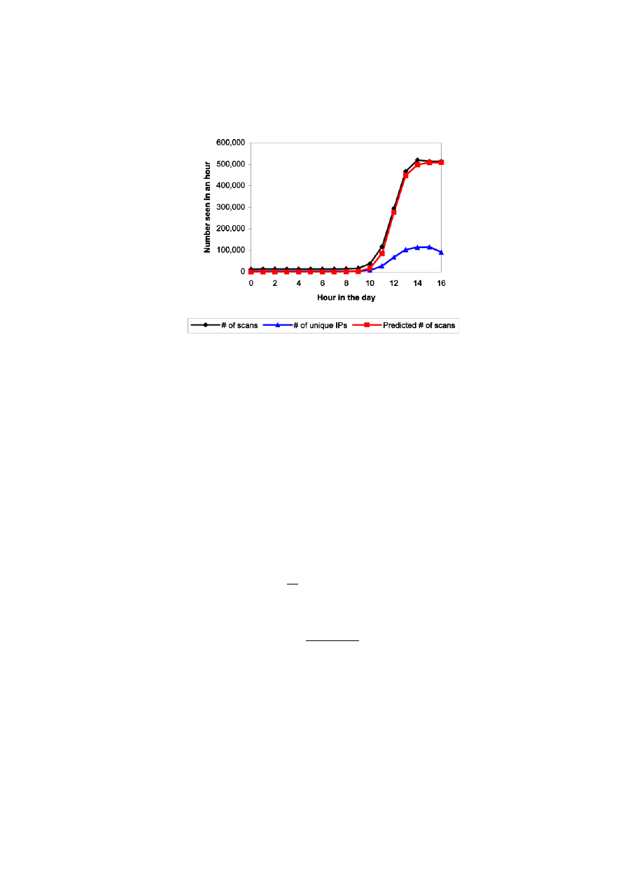
Fig. 1. Comparison between predicted and detected number of scans by Code Red, in
data offered by Chemical Abstracts Service; originally appeared in [5]

that will be compromised in the interval of time dt (in which we assume a to be
constant) is thus given by:

n = (N a) · K(1 − a)dt

(1)

We are obviously considering that, being 2

32

a very large address space, and

since CRv2 target list is truly random, the chance that two different instances
of the worm simultaneously try to infect a single target is negligible. Now, under
the hypothesis that N is constant, n = d(N a) = N da, we can also write:

N da = (N a) · K(1 − a)dt

(2)

From this, it follows the simple differential equation:

da

dt

= Ka(1 − a)

(3)

The solution of this equation is a logistic curve:

a =

e

K(t−T )

1 + e

K(t−T )

(4)

where T is a time parameter representing the point of maximum increase in the
growth. In [5] the authors fit their model to the “scan rate”, or the total number
of scans seen at a single site, instead than using the number of distinct attacker

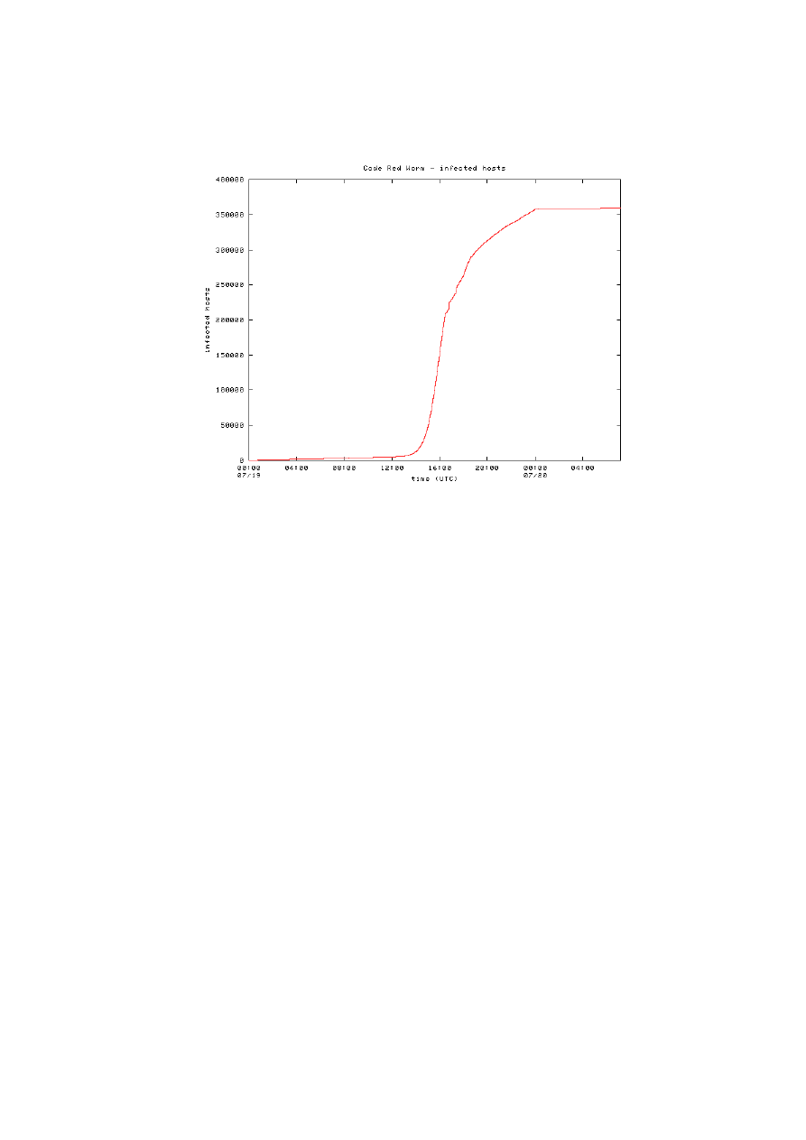
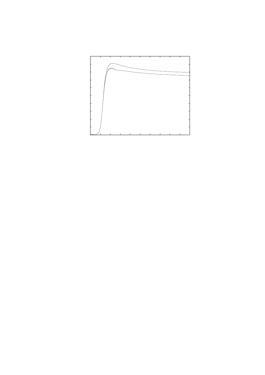
Fig. 2. The number of distinct IP addresses infected by Code Red v2 during its first
outbreak, drawn from [17]

IP addresses. We show this in Figure 1, where the logistic curve has parameters
K = 1.6 and T = 11.9. The scan rate is directly proportional to the total number
of infected IPs on the Internet, since each infected host has a fixed probability
to scan the observation point in the current time interval. On the contrary, the
number of distinct attacker addresses seen at a single site is evidently distorted
(as can be seen in Figure 1), since each given worm copy takes some random
amount of time before it scans a particular site. If the site covers just a small
address space, the delay makes the variable “number of distinct IP addresses of
attackers” to lag behind the actual rate of infection.

Researchers from CAIDA also published data on the Code Red outbreak [17];

their monitoring technique is based on the usage of a “network telescope” [18],
i.e. a large address-space block, routed but with no actual hosts connected. Three
of such telescope datasets (one observed from a /8 network, and two from /16
networks respectively) were merged to generate the data presented in the paper.
On such a large portion of IP space, the “distortion” is less evident, as we can
see in Figure 2. In Figure 3 the cumulative total of “attacker” IP addresses seen
by the telescopes is plotted on a log-log scale and fitted against the predictions of
the RCS model, on a logistic curve with parameter K = 1.8 and T = 16. CAIDA
data are expressed in the UTC timezone, while Chemical Abstracts Service data
were expressed in CDT timezone: this accounts for the different T parameter.

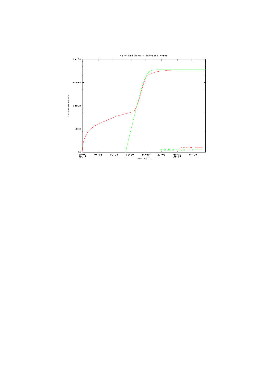
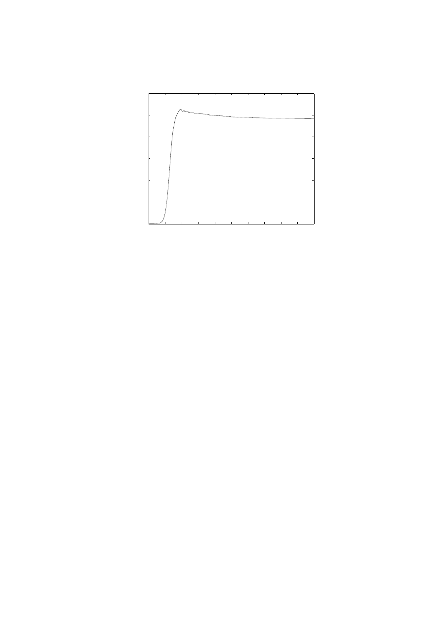
Fig. 3. The number of distinct IP addresses infected by Code Red v2 during its first
outbreak, plotted on a log-log scale and fitted against the RCS model, drawn from [17]

In Figure 4 instead we can see the deactivation rate of the worm, considering

as “deactivated” an host which did not attempt to spread the infection anymore.
The worm was built to deactivate its propagation routine on midnight of July
20, UTC time (to begin the Denial of Service process). This is clearly visible in
the graphic.

As we can see from Figures 3 and 1, at that time the worm was approaching

saturation. A total of about 359.000 hosts were infected by CRv2 in about 14
hours of activity (corresponding to the plateau in Figure 2).

In Figure 5 the hourly probe rate detected at the Chemical Abstracts Service

on day August 1st 2001 is compared to a fitting curve. On that day CRv2
reactivated after the denial of service cycle, as discussed before. CAIDA observes
that at peak 275.000 hosts were infected. The lower number is probably due to
ongoing patching activity during the 10-days grace period.

Other authors [19] propose the AAWP discrete time model, in the hope to

better capture the discrete time behavior of a worm. However, a continuous
model is appropriate for such large scale models, and the epidemiological liter-
ature is clear in this direction. The assumptions on which the AAWP model is
based are not completely correct, but it is enough to note that the benefits of
using a discrete time model seem to be very limited.

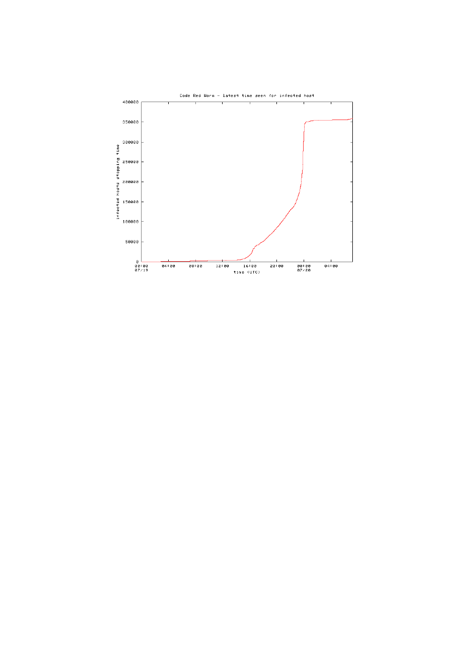
Fig. 4. Rate of “deactivation” of infected hosts, drawn from [17]

3

A new model for the propagation of worms on the
Internet

3.1

Slammer, or the crisis of traditional models

As described in section 2, a number of models have been developed for the prop-
agation of viruses and worms. However, most of them have critical shortcomings
when dealing with new, aggressive types of worms, called “flash” or “Warhol”
worms.

On Saturday, January 25th, 2003, slightly before 05:30 UTC, the Sapphire

Worm (also known as SQ-Hell or Slammer ) was released onto the Internet.
Sapphire propagated by exploiting a buffer overflow vulnerability in computers
on the Internet running Microsoft’s SQL Server or MSDE 2000 (Microsoft SQL
Server Desktop Engine). The vulnerability had been discovered in July 2002, and
a patch for it was actually available even before the vulnerability was announced.

The characteristic which made this worm so different from the previous ones

was its speed: it effectively showed a doubling time of 8.5(±1) seconds, infecting
more than 90 percent of vulnerable hosts within the first 10 minutes. It was thus
a lot faster than Code Red, which had a doubling time of about 37 minutes. At
least 75.000 hosts were infected by Sapphire.

Sapphire’s spreading strategy is based on random scanning, like Code Red.

Thus, the same RCS model that described CRv2 should fit also Sapphire’s

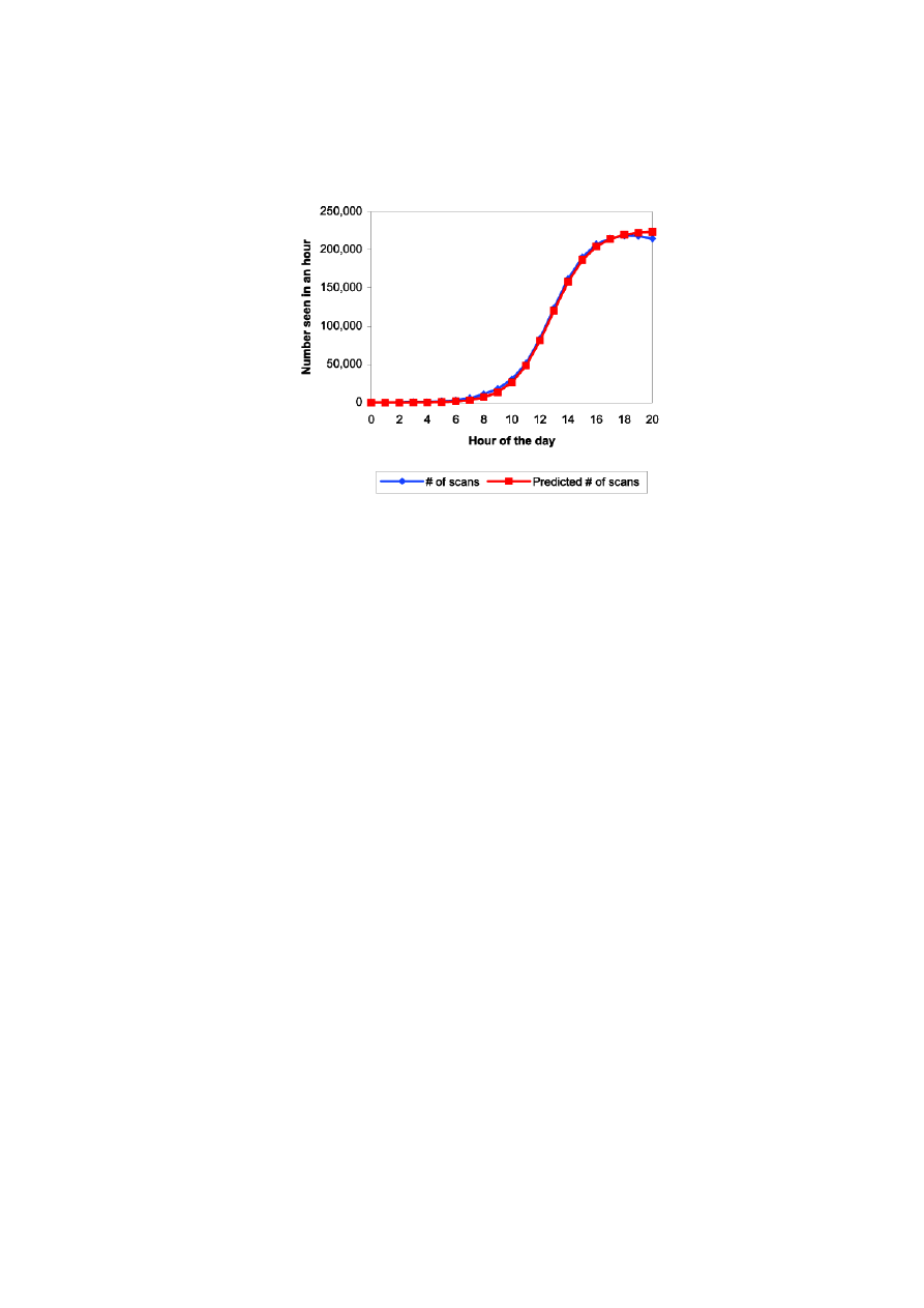
Fig. 5. The real and predicted scan rate of Code Red v2 during the second outbreak
on August 1st, as it appears in the CAS [5] dataset. The time of day is expressed in
Central US Time.

growth. However, as it appears from Figure 6, the model fits well only for the
initial stage of growth. Then, suddenly, there is an abrupt difference between
the model and the real data.

We must remember that this data shows the total number of scans, not the

actual number of infected machines. After approximately 3 minutes from the be-
ginning of the infection, the worm achieved its full scanning rate of more than 55
million scans per second; after this point, the rate of growth slowed down some-
what. The common explanation for this phenomenon is that significant portions
of the network did not have enough bandwidth to support the propagation of
the worm at its full speed: in other words, the worm saturated the network
bandwidth before saturating the number of infectable hosts.

Why was Sapphire so deadly efficient, when compared to Code Red? The

difference relies mainly in the transmission mechanism: the exploit used by Sap-
phire was based on UDP, while the exploit of Code Red was based on TCP. So,
Code Red had to establish a connection before actually exploiting the vulnera-
bility: having to complete the three-way handshake, waiting for answers, it was
latency limited. Sapphire, on the contrary, could scan at the full speed allowed
by the network bandwidth available, so it was network limited.

In order to properly model such a worm, the bandwidth between nodes must

be taken into account: this means that most of the proposed models are not
applicable in this situation because they use the “global reachability” property
of the Internet as a simplifying assumption.

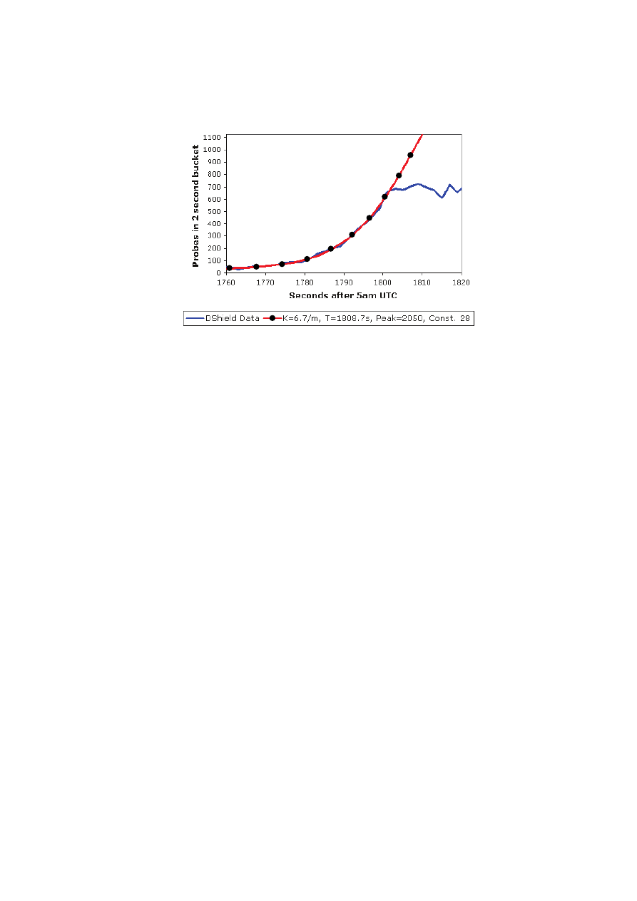
Fig. 6. The growth of Slammer scans, as seen from Dshield.org, fitted against the RCS
model; K, T and Const are the parameters of the fitting curve

3.2

Building a compartment-based model

Modeling the whole Internet as a graph, with each node representing an host,
is unfeasible. Even modeling the communication infrastructure, representing
routers as nodes of the graph and links as edges, is an almost impossible task.

Luckily, we do not need such granularity. The Internet can be macroscop-

ically thought of as the interconnection of a number of Autonomous Systems.
An AS is a subnetwork which is administered by a single authority. Usually, the
bottlenecks of Internet performance are located in the inter-AS connections (i.e.
the peering networks and the NAP connections), not in the intra-AS connec-
tions. However, some AS are instead very large entities, which comprise densely
connected regions and bottleneck links: in this case we could split these ASs in
smaller regions that satisfy the property.

For this reason, we propose a compartment-based model, in which we suppose

that inside a single autonomous system (or inside a densely connected region of
an AS) the worm propagates unhindered, following the RCS model described in
Section 2.3. However, we wish to model the behavior of the worm in the intra-AS
propagation, and for this purpose we need to rewrite and extend Equation 3.

Let N

i

be the number of susceptible hosts in the i-th AS (AS

i

), and a

i

the

proportion of infected hosts in the same AS. Now, let us suppose that K is the
average propagation speed of the worm, and in first approximation let us say it
is constant in every single AS. Let P

IN,i

be the probability that a host inside

AS

i

targets an host inside the same AS, and P

OU T,i

the probability that instead

it attacks another AS.

In a simple model with just two autonomous systems, the following equation

describes both the internal and external worm infection attempts on AS

1

:

N

1

da

1

=





N

1

a

1

KP

IN,1

dt

|

{z

}

Internal

+ N

2

a

2

KP

OU T,2

dt

|

{z

}

External





 (1 − a

1

)

A similar equation can obviously be drawn for AS

2

simply by switching the

terms. We thus have a system of two differential equations:







da

1

dt

=

h

a

1

KP

IN,1

+

N

2

N

1

a

2

KP

OU T,2

i

(1 − a

1

)

da

2

dt

=

h

a

2

KP

IN,2

+

N

1

N

2

a

1

KP

OU T,1

i

(1 − a

2

)

Under the assumption that the worm randomly generates the target IP ad-

desses, it follows that P

IN,1

= N

1

/N and P

OU T,1

= 1 − P

IN,1

= N

2

/N . Substi-

tuting these values, and extending the result to a set of n ASs, we obtain the
following system of n differential equations:











da

i

dt

=





a

i

K

N

i

N

+

n

P

j=1
j6=i

N

j

N

i

a

j

K

N

i

N





 (1 − a

i

) 1 ≤ i ≤ n

(5)

We can think of the result of the integration of each equation as a logistic

function (similar to the one generated by the RCS model), somehow “forced” in
its growth by the second additive term (which represents the attacks incoming
from outside the AS).

Simplifying the equation we obtain:



































da

i

dt

=



















a

i

K

N

i

N

+

n

X

j=1
j6=i

N

j

N

a

j

K

|

{z

}

incoming attacks



















(1 − a

i

)

(6)

in which we left in evidence the term describing the incoming attack rate, but
we can further reduce the equations to the following:







da

i

dt

=





n

X

j=1

N

j

a

j



 (1 − a

i

)

K
N

(7)

This is a nonlinear system of differential equations. It can be easily shown

that the results of equation 7 are a solution also for this model, with the same

K and N parameters. Considering that a =

n

P

i=1

N

i

a

i

N

, we have:

da

dt

=

d

dt









n

P

i=1

N

i

a

i

N







 =

1

N

n

X

i=1

N

i

da

i

dt

and, from equation 7:

da

dt

=

1

N

n

X

i=1







N

i





n

X

j=1

N

j

a

j



 (1 − a

i

)

K
N







=

K

N

2

n

X

i=1

N

i

N a (1 − a

i

) =

=

a K

N

n

X

i=1

N

i

(1 − a

i

) =

a K

N

"

n

X

i=1

N

i

−

n

X

i=1

N

i

a

i

#

=

a K

N

[N − N a] =

= a K (1 − a)

Thus we obtain equation 3.
We can explore the solutions of a linearization of the system, in the neigh-

borhood of the unstable equilibrium point in a

j

= 0, ∀j. With the convention of

using the newtonian notation (denoting the first derivative with an upper dot),
and using the traditional substitution of a

i

= (a

i

+ δa

i

), we obtain:























•

(a

i

+ δa

i

) =









X

j

N

j

a

j



 (1 − a

i

)

K
N





¯

¯

¯

¯

¯

¯

a

+

∂

Ã"

P

j

N

j

a

j

#

(1 − a

i

)

K
N

!

∂a

i

¯

¯

¯

¯

¯

¯

¯

¯

¯

¯

a

δa

i







•

δa

i

=









X

j

N

j

a

j



 (1 − a

i

)

K
N



 +



−





X

j

N

j

a

j



 + N

i

(1 − a

i

)



 K

N

δa

i

Now we can inject a small number of worms in the k-th autonomous system,

in a model initially free of virus infections: a

i

= 0; δa

k

(0) = 0, ∀i 6= k; δa

k

(0) =

ε > 0. The system initially behaves in this way:

½

•

δa

i

= N

i

K
N

δa

i

Thus, in the k-th autonomous system, the worm begins to grow according

to the RCS model, while the other AS are temporarily at the equilibrium. This
state, however, lasts only until the worm is first “shot” outside the AS, which
happens a few moments after the first infection.

We can now calculate analytically the bandwidth consumed by incoming

attacks on a “leaf” AS, AS

i

, connected to the network via a single connection

(a single homed AS). Let s be the size of the worm, r

j

the number of attacks

generated in a time unit by AS

j

. Let T describe the total number of systems

present on the Internet, and T

i

the number of systems in AS

i

. The rate of attacks

that a single infected host performs in average is R ∼

= K

T

N

(since K is the rate

of successful outgoing attacks). The incoming bandwidth b

i,incoming

wasted by

the incoming worms on the link is therefore described by:

b

i,incoming

= s

n

X

j=1
j6=i

r

j

T

i

T

= s

n

X

j=1
j6=i

a

j

N

j

R

T

i

T

= s

n

X

j=1
j6=i

a

j

N

j

K T

N

T

i

T

= s K

T

i

N

n

X

j=1
j6=i

a

j

N

j

(8)

If we compare equations 8 and 6, we can see the structural analogy:

b

i,incoming

= s T

i

n

X

j=1
j6=i

N

j

N

a

j

K

|

{z

}

incoming attacks

(9)

We must also consider the outgoing attack rate, which equals the generated

attacks minus the attacks directed against the AS itself:

b

i,outgoing

= sr

i

·

1 −

T

i

T

¸

= s a

i

N

i

R

·

1 −

T

i

T

¸

= s a

i

N

i

K

T

N

·

T − T

i

T

¸

Also in this case we can see a structural analogy with equation 6:

b

i,outgoing

= s (T − T

i

)

a

i

N

i

N

K

| {z }

outgoing attacks

(10)

Adding equation 9 to equation 10 we can thus obtain the amount of band-

width the worm would waste on AS

i

if unconstrained:

b

i

= s (T − T

i

) a

i

N

i

N

K + s T

n

X

j=1
j6=i

N

j

N

a

j

K

(11)

Considering that:

a

i

N

i

N

K +

X

j6=i

N

j

N

a

j

K =

X

j

N

j

N

a

j

K

we can easily see that:

b

i

= s(T − T

i

)a

i

N

i

N

K + s T





X

j

N

j

N

a

j

K − a

i

N

i

N

K



 =

= s T

X

j

N

j

N

a

j

K − s T

i

a

i

N

i

N

K =

s K

N



T

X

j

N

j

a

j

− T

i

a

i

N

i





We could also extend this result to a multi-homed leaf AS, that is, an AS

with multiple connections to the Internet, but which does not carry traffic from
one peer to another for policy reasons (as it is the case for many end-user sites).
We must simply divide this equation, using a different equation for each link,
each carrying the sum of the AS that are reachable through that link. We should
also rewrite equation 10 to split up the outgoing attacks depending on the links.
This would not change the overall structure of the equations.

It would be a lot more complex to model a non-leaf AS, because we should

take into account also the incoming and outgoing traffic on each link that is being
forwarded from a neighbor AS to another. The complexity lies in describing in a
mathematically tractable way the paths on a complex network. However, we can
ignore, in first approximation, non-leaf AS, because they tend to be carriers of
traffic, not containing hosts susceptible to the worm: they can thus be considered
as a part of the intra-AS connection links.

Let us go back to the leaf, single-homed model, and let us suppose now that

there is a structural limit to the available bandwidth on the link, B

i

. In the

simplest possible model, we will see that only a fraction Q

i

, 0 < Q

i

≤ 1 of

packets will be allowed to pass through the i-th link, such that Q

i

b

i

≤ B

i

. The

actual behavior of the system under an increasing load is not known a priori,
but we can suppose that there exists a simple relation expressing the saturation
of the link, such as:

B

i

( 1 − e

−λ

bi

Bi

) = Q

i

b

i

⇒ Q

i

=

B

i

( 1 − e

−λ

bi

Bi

)

b

i

This is justified by thinking that:

lim

b

i

→0

B

i

( 1 − e

−λ

bi

Bi

) = 0 lim

b

i

→+∞

B

i

( 1 − e

−λ

bi

Bi

) = B

i

Resubstituting this:

Q

i

b

i

= Q

i



s (T − T

i

) a

i

N

i

N

K + s T

X

j6=i

N

j

N

a

j

K



 =

0

5

10

15

20

25

30

35

40

45

50

0

0.1

0.2

0.3

0.4

0.5

0.6

0.7

0.8

0.9

1

Time

Inf

ec

tion r

a

tio (a)

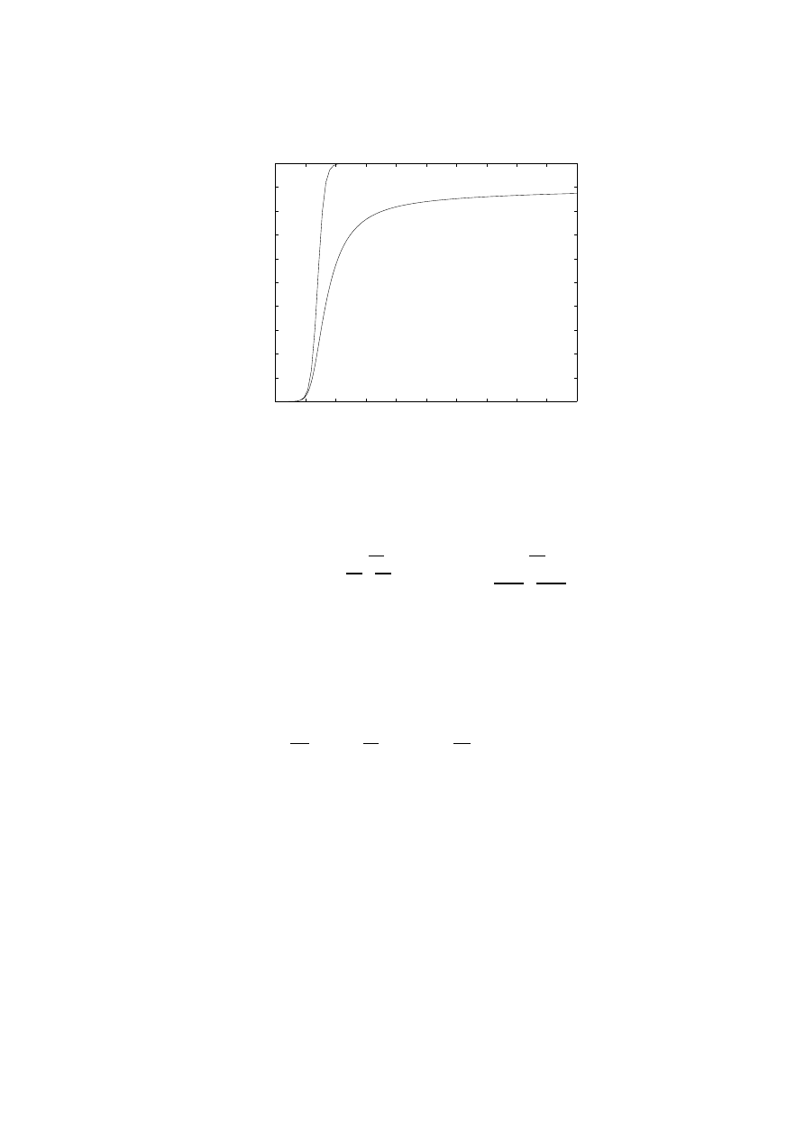
Fig. 7. A comparison between the unrestricted growth predicted by an RCS model and
the growth restricted by bandwidth constraints

= s (T − T

i

)









Q

i

a

i

N

i

N

K

|

{z

}

reduced outgoing rate







 + s T















Q

i

X

j6=i

N

j

N

a

j

K

|

{z

}

reduced incoming rate















As we see, in order to reduce the bandwidth to the value Q

i

b

i

, and under

the hypothesis that the incoming and outgoing stream of data are curtailed by
the same factor, the incoming and outgoing attack rate must be decreased of
this same factor Q

i

. We can now substitute this reduced attack rate into the

system of equations 6 (remembering that the inner worm propagation will be
unaffected), and thus obtain:







da

i

dt

=



a

i

K

N

i

N

+ Q

i

X

j6=i

Q

j

N

j

N

a

j

K



 (1 − a

i

)

(12)

Equation 12 expresses the same model, but with a limit on the dataflow rate

of the links between different ASs. We have plotted this equation using Simulink
and Matlab, obtaining the result shown in Figure 7. Here we compare the dif-
ferent results of equations 6 and 12. They are built with the same parameters,
and thus their initial growth is totally symmetric. However, as soon as the links
begin to saturate, the growth of equation 12 slows down.

We can then insert into the Simulink model an additional component in order

to simulate the disruption in the Internet links caused by traffic overload. In

0

5

10

15

20

25

30

35

40

45

50

0

0.5

1

1.5

2

2.5

3

3.5

4

4.5

5

x 10

4

At

ta

ck R

a

te

Time

Fig. 8. Attack rates observed on a single link, under the hypotheses that links hold
(upper curve) or randomly fail (lower curve)

particular, we suppose that a proportion p of the links will shut down when they
are flooded by worm traffic (i.e. when the worm generates a flow of packets a lot
above B

i

). In Figure 8 we see the comparison on the traffic observed on a single

link with or without this additional detail. We can observe the small oscillations
that are generated, even in this static and simplified model of network failure.

We repeated our simulations for a variety of parameters of the model, con-

cluding that as the bandwidth limit increases the small peak of traffic seen on
the link is less and less evident, up to the point where the model behaves ex-
actly as if the bandwidths were unlimited. Increasing the number of failing links,
instead, increases the oscillations after the peak.

In Figure 9 we instead plot the number of attacks seen on a large subset of

the links. This is very similar to the behavior observed by DShield during the
Slammer outbreak (see Figure 6): DShield, in fact, monitors a large subset of
different links. However, as can be seen in Figure 7, the actual growth of the
worm is only slowed down, not stopped at all, by the vanishing links.

In our opinion, then, the sudden and strange stop in the increase of observed

attacks can indeed be explained by the disruption of Internet links, as hypothe-
sized in various previous works, but this does not imply a similar slow down in
the growth of the worm.

0

5

10

15

20

25

30

35

40

45

50

0

1

2

3

4

5

6

x 10

7

Time

At

ta

ck R

a

te

Fig. 9. The number of attack rates seen by a global network telescope, under the
hypothesis that some links fail during the outbreak

4

A discussion of proposed countermeasures

4.1

Monitoring and early warning

In [20] the authors use the models of active worm propagation to describe a
monitoring and alerting system, based on distributed ingress and egress sensors
for worm activity. Ingress sensors detect as possible worm activity any incoming
scan trying to contact unused addresses on the network (with a principle similar
to the one of the network telescopes discussed in section 2.3). Egress sensors
instead try to capture outgoing worm activity from the network.

In order to create a global early warning distributed sensor network, the

authors propose a data collection engine, capable of correcting the statistical
biases responsible for the distortions described in section 2.3. They propose the
use of a Kalman filter for estimating parameters such as K, N and a from the
observations, and thus have a detailed understanding of how much damage the
spreading worm could generate. In addition, using some properties of the filter,
it can be used to generate and early warning of worm activity as early as when
1% ≤ a ≤ 2%.

The authors also show that this early warning method works well also with

fast spreading worms, and even if an hit-list startup strategy is used.

4.2

Modeling removal and disinfection of hosts

Models such as RCS purposefully avoid to take into account the dynamics of
countermeasures deployed to stop or contain virus outbreaks, considering worm
propagation to be too quick to be influenced by human response.

A study by Zou et al. [21], focused on slower propagating worms such as Code

Red, builds upon the RCS equations, incorporating the Kermack-Mckendrick
model which accounts for the removal of infectious hosts, and extending it to
the removal of susceptible hosts as well.

Additionally, the authors propose that the infection rate K should be con-

sidered a function of time: K = K(t), because of intervening network saturation
and router collapse. Basically they rewrite the model as:

da

dt

= K(t) a (1 − a − q − r) −

dr

dt

(13)

Where q(t) is the proportion of susceptible hosts that are immunized at time

t, and r(t) is the proportion of infected hosts that are cured and immunized at
time t. This model is called the two-factor worm model. In order to completely
describe the model, the authors make some assumptions on q(t) and r(t). In
particular, they hypothesize that a constant portion of the infected machines
are cured on a unit of time:

dr

dt

= γa

Additionally, with an hypothesis close to the kill signal theory described by

Wang et al. in [22], they describe the patching process as a diffusion similar to
the one of the worm:

dq

dt

= µ(1 − a − q − r)(a + r)

it is unclear, however, how the authors chose this particular equation, and

how the variables have been chosen. Also, as it has been pointed out in comments
to the paper by Wang et al., it is far from evident that the kill signal propagation
and the worm propagation follow the same parameters, or even the same topol-
ogy of network. However the simulation of this model yields interesting analogies
with the real data of the Code Red outbreak.

A model by Wang et al. [23] shows the interdependence between the tim-

ing parameters of propagation and removal, and their influence on the worm
propagation.

4.3

Quarantine: the world’s oldest defense

In [24] the authors study a dynamic preventive quarantine system, which places
suspiciously behaving hosts under quarantine for a fixed interval of time. We
omit many details of their analysis, but their conclusion is as follows. Let 1/λ

1

be the mean time before an infected host is detected and quarantined, 1/λ

2

be

the mean time before a false positive occurs, i.e. a non-infected host is wrongly
quarantined, and T be the quarantine time.

The probability that an infectious host is correctly quarantined is

p

1

=

λ

1

T

1 + λ

1

T

and the probability of a false positive conversely is:

p

2

=

λ

2

T

1 + λ

2

T

So the RCS model may be applied, by discounting the infection rate K in

order to take into account the effects of quarantine:

K

0

= (1 − p

1

)(1 − p

2

)K

An extension of the Kermack-Mckendrick model, omitted here for brevity, is also
presented, and the results of simulation runs on both these models are discussed.

It should be noted that such a dynamic quarantine system would be difficult

to implement, because each host cannot be trusted to auto-quarantine itself.
Practically, on most networks, the number of remotely manageable enforcement
points (i.e. firewalls and intelligent network switches) is limited. Entire blocks of
network would need to be isolated at once, uncontrollably increasing the factor
p

2

. This could help to stop the warm, but with a steep price, since p

2

represents

the probability that innocent hosts will be harmed by quarantine.

In addition, as shown by the model presented in 3.2, the virus spread is

not stopped but only slowed down inside each quarantined block. Moreover, it
should be considered that the “kill signal” effect (i.e. the distribution of anti-virus
signatures and patches) would be hampered by aggressive quarantine policies.

On the same topic Moore et al. [25] simulated various containment strategies

(namely content filtering and blacklisting), deriving lower and upper bounds of
efficacy for each. Albeit interesting, the results on blacklisting share the same
weakness pointed out before: it’s not realistic to think about a global blacklisting
engine.

Real-world isolation techniques are far less efficient. On a LAN, an intelligent

network switch could be used to selectively shut down the ports of infected hosts,
or to cut off an entire sensitive segment. Network firewalls and perimeter routers
can be used to shut down the affected services. Reactive IDSs (the so-called
“intrusion prevention systems”) can be used to selectively kill worm connections
on the base of attack signatures.

Automatic reaction policies are intrinsically dangerous. False positives and

the possibility of fooling a prevention system into activating a denial-of-service
are dangerous enough to make most network administrators wary.

4.4

Immunization

In [22] the effect of selective immunization of computers on a network is dis-
cussed. The dynamics of infection and the choice of immunization targets are

examined for two network topologies: a hierarchical, tree-like topology (which is
obviously not realistic for modeling the Internet), and a cluster topology. The
results are interesting, but the exact meaning of “node immunization” is left
open.

If it means the deployment of anti-virus software, as we discussed before, it

consists of a reactive technology which cannot prevent the spread of malicious
code. If it means the accurate deployment of patches, the study could be used
to prioritize the process, in order to patch sooner the most critical systems.

4.5

Honeypots and tarpits

Honeypots are fake computer system and networks, used as a decoy to delude
intruders. They are installed on dedicated machines, and left as a bait so that
aggressors will lose time attacking them and trigger an alert. Since honeypots
are not used for any production purpose, any request directed to the honey-
pot is at least suspect. Honeypots can be made up of real sacrificial systems,
or of simulated hosts and services (created using Honeyd by Niels Provos, for
example).

An honeypot could be used to detect the aggressive pattern of a worm (either

by attack signatures, or by using a technique such as the one described above).
When a worm is detected, all the traffic incoming from it can be captured at the
gateway level and routed to a fake version of the real network.

Using signatures has the usual disadvantage that they may not be readily

available for an exploding, unknown worm. Using anomaly detection filters is
prone to false positives, and could send legitimate traffic into the fake honeypot.

Once a worm has entered a honeypot, its payload and replication behaviors

can be easily studied, without risk. An important note is that hosts on the
honeypot must be quarantined and made unable to actually attack the real
hosts outside. By using sacrificial unprotected machines, copies of the worm can
be captured and studied; sometimes, even using honeyd with some small tricks
is sufficient in order to capture copies of the worm.

As an additional possibility, an honeypot can be actually used to slow down

the worm propagation, particularly in the case of TCP based worms. By delaying
the answers to the worm connections, a honeypot may be able to slow down its
propagation: when a copy of the worm hits the honeypot, it sees a simulated
open TCP port, and thus it is forced to attack the fake host, losing time in the
process.

This technique is used in the Labrea “tarpit” tool. LaBrea can reply to any

connection incoming on any unused IP address of a network, and simulate a TCP
session with the possible aggressor. Afterward it slows down the connection:
when data transfer begins to occur, the TCP window size is set to zero, so no
data can be transferred. The connection is kept open, and any request to close
the connection is ignored. This means that the worm will have to wait for a
timeout in order to disconnect, since it uses the standard TCP stack of the
host machine which follows RFC standards. A worm won’t be able to detect

this slowdown, and if enough fake targets are present, its growth will be slowed
down. Obviously, a multi-threaded worm will be less affected by this technique.

4.6

Counterattacks and good worms

Counter-attack may seem a viable cure to worms. When an host A sees an
incoming worm attack from host B, it knows that host B must be vulnerable
to the particular exploit that the worm uses to propagate, unless the worm
itself removed that vulnerability. By using the same type of exploit, host A can
automatically take control of host B and try to cure it from infection and patch
it.

The first important thing to note is that, fascinating as the concept may seem,

this is not legal, unless host B is under the control of the same administrator of
host A. Additionally, automatically patching a remote host is always a dangerous
thing, which can cause considerable unintended damage (e.g. breaking services
and applications that rely on the patched component).

Another solution which actually proves to be worse than the illness is the

release of a so-called “good” or “healing” worm, which automatically propagates
in the same way the bad worm does, but carries a payload which patches the
vulnerability. A good example of just how dangerous such things may be is the
Welchia worm, which was meant to be a cure for Blaster, but actually caused
devastating harm to the networks.

5

Conclusions and future work

In this paper, we reviewed existing modeling techniques for computer virus prop-
agation, presenting their underlying assumptions, and discussing whether or not
these assumptions can still be considered valid. We also presented a new model,
which extends the Random Constant Spread model, which allows us to derive
some conclusions about the behavior of the Internet infrastructure in presence
of a self-replicating worm. We compared our modeling results with data col-
lected during the outbreak of the Slammer worm and proposed an explanation
for some observed effects. We also discussed briefly countermeasures for fighting
a self-replicating worm, along with their strengths and weaknesses. As a future
extension of this work, we will try to model these countermeasures in order to
assess their value in protecting the Internet infrastructure.

6

Acknowledgments

We thank David Moore of CAIDA, and Stuart Staniford of Silicon Defense,
for allowing us to reproduce their measurements of Code Red v2 expansion.
We also wish to thank Sergio Savaresi, Giuliano Casale and Paolo Albini for
reading a preliminary version of the equations in section 3.2 and providing helpful
suggestions for the improvement of the model.

References

1. Cohen, F.: Computer Viruses. PhD thesis, University of Southern California (1985)
2. Cohen, F.: Computer viruses – theory and experiments. Computers & Security 6

(1987) 22–35

3. Power, R.: 2003 csi/fbi computer crime and security survey. In: Computer Security

Issues & Trends. Volume VIII. Computer Security Institute (2002)

4. White, S.R.: Open problems in computer virus research. In: Proceedings of the

Virus Bulletin Conference. (1998)

5. Staniford, S., Paxson, V., Weaver, N.: How to 0wn the internet in your spare time.

In: Proceedings of the 11th USENIX Security Symposium (Security ’02). (2002)

6. Whalley, I., Arnold, B., Chess, D., Morar, J., Segal, A., Swimmer, M.: An envi-

ronment for controlled worm replication and analysis. In: Proceedings of the Virus
Bulletin Conference. (2000)

7. Spafford, E.H.: Crisis and aftermath. Communications of the ACM 32 (1989)

678–687

8. Kephart, J.O., White, S.R.: Directed-graph epidemiological models of computer

viruses. In: IEEE Symposium on Security and Privacy. (1991) 343–361

9. Hethcote, H.W.: The mathematics of infectious diseases. SIAM Review 42 (2000)

599–653

10. Billings, L., Spears, W.M., Schwartz, I.B.: A unified prediction of computer virus

spread in connected networks. Physics Letters A (2002) 261–266

11. Zou, C.C., Towsley, D., Gong, W.: Email virus propagation modeling and analysis.

Technical Report TR-CSE-03-04, (University of Massachussets, Amherst)

12. Permeh, R., Maiffret, M.: .ida ’code red’ worm. Advisory AL20010717 (2001)
13. Permeh, R., Maiffret, M.: Code red disassembly. Assembly code and research paper

(2001)

14. Permeh, R., Hassell, R.:

Microsoft i.i.s. remote buffer overflow.

Advisory

AD20010618 (2001)

15. Levy, E.A.: Smashing the stack for fun and profit. Phrack magazine 7 (1996)
16. Craig Labovitz, A.A., Bailey, M.: Shining light on dark address space. Technical

report, Arbor networks (2001)

17. Moore, D., Shannon, C., Brown, J.: Code-red: a case study on the spread and

victims of an internet worm. In: Proceedings of the ACM SIGCOMM/USENIX
Internet Measurement Workshop. (2002)

18. Moore, D.: Network telescopes: Observing small or distant security events. In:

Proceedings of the 11th USENIX Security Symposium. (2002)

19. Chen, Z., Gao, L., Kwiat, K.: Modeling the spread of active worms. In: Proceedings

of IEEE INFOCOM 2003. (2003)

20. Zou, C.C., Gao, L., Gong, W., Towsley, D.: Monitoring and early warning for

internet worms. In: Proceedings of the 10th ACM conference on Computer and
communication security, ACM Press (2003) 190–199

21. Zou, C.C., Gong, W., Towsley, D.: Code red worm propagation modeling and anal-

ysis. In: Proceedings of the 9th ACM conference on Computer and communications
security, ACM Press (2002) 138–147

22. Wang, C., Knight, J.C., Elder, M.C.: On computer viral infection and the effect

of immunization. In: ACSAC. (2000) 246–256

23. Wang, Y., Wang, C.: Modelling the effects of timing parameters on virus propaga-

tion. In: Proceedings of the ACM CCS Workshop on Rapid Malcode (WORM’03).
(2003)

24. Zou, C.C., Gong, W., Towsley, D.: Worm propagation modeling and analysis under

dynamic quarantine defense. In: Proceedings of the ACM CCS Workshop on Rapid
Malcode (WORM’03). (2003)

25. Moore, D., Shannon, C., Voelker, G.M., Savage, S.: Internet quarantine: Require-

ments for containing self-propagating code. In: INFOCOM. (2003)